Simulation of thermal field in soil - itep.edu.pl I i in... · PROBLEMS OF AGRICULTURAL ENGINEERING s.57–65 ... Jan Rados ław KAMIŃSKI2) DEF ... simulation of soil thermal field

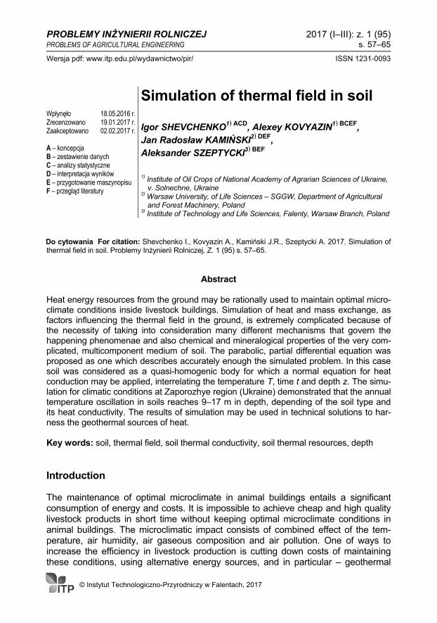
PROBLEMY INŻYNIERII ROLNICZEJ 2017 (I–III): z. 1 (95) PROBLEMS OF AGRICULTURAL ENGINEERING s. 57–65

Wersja pdf: www.itp.edu.pl/wydawnictwo/pir/ ISSN 1231-0093

© Instytut Technologiczno-Przyrodniczy w Falentach, 2017

Wpłynęło 18.05.2016 r. Zrecenzowano 19.01.2017 r. Zaakceptowano 02.02.2017 r.

A – koncepcja B – zestawienie danych C – analizy statystyczne D – interpretacja wyników E – przygotowanie maszynopisu F – przegląd literatury

Simulation of thermal field in soil

Igor SHEVCHENKO1) ACD, Alexey KOVYAZIN1) BCEF,Jan Radosław KAMIŃSKI2) DEF,Aleksander SZEPTYCKI3) BEF

1) Institute of Oil Crops of National Academy of Agrarian Sciences of Ukraine,v. Solnechne, Ukraine

2) Warsaw University, of Life Sciences – SGGW, Department of Agriculturaland Forest Machinery, Poland

3) Institute of Technology and Life Sciences, Falenty, Warsaw Branch, Poland

Do cytowania For citation: Shevchenko I., Kovyazin A., Kamiński J.R., Szeptycki A. 2017. Simulation of thermal field in soil. Problemy Inżynierii Rolniczej. Z. 1 (95) s. 57–65.

Abstract

Heat energy resources from the ground may be rationally used to maintain optimal micro-climate conditions inside livestock buildings. Simulation of heat and mass exchange, as factors influencing the thermal field in the ground, is extremely complicated because of the necessity of taking into consideration many different mechanisms that govern the happening phenomenae and also chemical and mineralogical properties of the very com-plicated, multicomponent medium of soil. The parabolic, partial differential equation was proposed as one which describes accurately enough the simulated problem. In this case soil was considered as a quasi-homogenic body for which a normal equation for heat conduction may be applied, interrelating the temperature T, time t and depth z. The simu-lation for climatic conditions at Zaporozhye region (Ukraine) demonstrated that the annual temperature oscillation in soils reaches 9–17 m in depth, depending of the soil type and its heat conductivity. The results of simulation may be used in technical solutions to har-ness the geothermal sources of heat.

Key words: soil, thermal field, soil thermal conductivity, soil thermal resources, depth

Introduction

The maintenance of optimal microclimate in animal buildings entails a significant consumption of energy and costs. It is impossible to achieve cheap and high quality livestock products in short time without keeping optimal microclimate conditions in animal buildings. The microclimatic impact consists of combined effect of the tem-perature, air humidity, air gaseous composition and air pollution. One of ways to increase the efficiency in livestock production is cutting down costs of maintaining these conditions, using alternative energy sources, and in particular – geothermal

Igor Shevchenko, Alexey Kovyazin, Jan Radosław Kamiński, Aleksander Szeptycki

58 © ITP w Falentach; PIR 2017 (I–III): z. 1 (95)

energy [DYJAKON, MILA 2013; KREIS-TOMCZAK 2008; ONISZK-POPŁAWSKA i in. 2011; SZULC, ŁASKA 2012]. For the rational use of potential energy of soils with the application of technical equipment, having ground heat exchangers as working elements, it is necessary to determine the temperature field formed by various factors (Fig. 1). In doing so, first and foremost we need to calculate the temperature field of soil (that is to say, in the absence of thermal action on the soil of ground heat exchange system), which will be taken into account in the simulation of technological processes and technical sys-tems capable of using geothermal energy.

Source: own elaboration. Źródło: opracowanie własne. Fig. 1. Soil thermal field forming factors Rys. 1. Czynniki wpływające na pole rozkładu ciepła w gruncie DENISOVA [2003], GRZYBEK, PAWLAK [2015a, b], POLJANIN [2001] and other authors provide the dependencies which can be used for determination of thermal field in soils. However, these dependencies do not consider Earth's radiogenic heat flux of 65–101 mW·m–2 [POLLACK et al. 1993] for continental regions, including Ukraine's territory, which results in the steady increase in the soil temperature of 3°C for every 100 m of depth on the average [KAVANAUGH, RAFFERTY 1997; PABIS 2011].

Radiation, evaporation, convection from the soil

surface Promieniowanie, ulatnianie,

konwekcja z powierzchni gleby

Parameters and operation mode of ground heat exchangers

Parametry i działanie gruntowych wymienników ciepła

Thermal and physical characteristics of soil Termiczne i fizyczne

właściwości gleby


© ITP w Falentach; PIR 2017 (I–III): z. 1 (95) 59

CHROMOV, PETROSJANC [2006] and NERPIN, CHUDNOVSKIJ [1967] provide the follo-wing expression for thermal field in soil that allows us to consider Earth's radiogenic heat flow:

Θ

π

Θ

π),(

Θ

π

g

z

Тga

ztsineАtzT2ga

+ (z) (1)

where: Tg (z, t) = the soil temperature at time t and depth z [С]; АТ = amplitude of the soil surface temperature (at z = 0) [С]; аg = thermal conductivity of the soil [m2·month–1]; = amplitude cycle, = 12 months; (z) = function describing the distribution of temperature in the ground with depth

at the initial moment of time, which can be used to calculate Earth's radio-genic heat flow.

The problem was solved with given initial condition: Tg (z, 0) = (z) and boundary

conditions: Tg (, t) = 0;

00 tt2

sinАtT ТgΘ

π),( , where t0 is the initial phase.

However, the above reference does not provide a detailed derivation of the expression (1), and what is more, the derived expression satisfies neither the initial condition nor the boundary conditions at the soil surface, what can be proved by direct substitution.

Results of investigations

Simulation of heat and mass transfer, which is a factor of thermal field formation in such a multi-component system as soil, is a highly complicated task because of the necessity of considering mathematical description and implementation of various mechanisms: thermal conductivity of solids, heat transfer from one solid particle to another upon their contact, molecular thermal conductivity of the medium that fills the space between solid particles, convection of steam and water occupying the pore space, and so on. Strictly speaking, besides the aforesaid mechanisms, the simulation of soil thermal field requires the consideration of chemical and miner-alogical characteristics of the soil skeleton, mechanical properties of solids, disper-sion degree in porous medium, shape and size of solids and pores, number of phases, quantitative relationship between phases and their relative position in the porous medium and many other physical and chemical parameters of the soil. The detailed consideration of the aforesaid factors in simulation of soil thermal fields represents a serious problem [KOLPAKOV 2016; VASILEV 2006].

However, applying the model of equivalent thermal conductivity we can to describe those processes accurately enough by means of the parabolic partial differential equation using equivalent coefficients [CHUDNOVSKIJ 1976]. In this case, the soil is considered as a quasi-homogeneous body for which an ordinary heat conduction equation, relating temperature Тg, time t and depth z, can be applicable.



2

2

z

Ta

t

T gg

g

(2)

The soil thermal field can be determined based upon a solution of the basic equation (2) with preset boundaries, that is the initial and boundary conditions.

The initial condition is defined by using the function of temperature distribution with depth of the earth at the initial moment of time:

zkТzT Tg 00 g (3)where: Тg0 = average annual temperature at the soil surface [С]; kT = the rate of temperature increase with depth depending on the rate of

Earth's radiogenic heat flow, can be taken as kT = 0,03С·m–1 for thermal conditions of Ukraine.

Boundary conditions expressing the law of soil-environment interactions, should be formulated as two soil boundaries.

The boundary condition at the soil surface can be written as follows:

tsinАТtT ТggΘ

π),(

20 0 (4)

The amplitude of temperature oscillations decay with depth, and when the value z Z is reached, the soil temperature remains practically unchangeable in the pre-scribed time interval, that allows the setting of the following boundary condition [CHUDNOVSKIJ 1976]:

constZkТtZT Tgg 0 (5)

According to CHROMOV and PETROSJANC [2006], annual temperature-oscillations decay in amplitude towards zero at a depth of 30 m in polar latitudes, at a depth of 15–20 m in mid-latitudes, and about 10 m in tropical latitudes (where annual ampli-tudes have lower values then in middle latitudes). At these depths the annual soil temperature remains constant.

Therefore, Z = 100 taken for the boundary condition (5) will guarantee the absence of temperature oscillations at this depth and lead to lower computational costs to an acceptable level.

The soil surface temperature for Zaporozhye region was determined as a function of time using “Scientific-practical handbook of SSSR climate” [Gidrometeoizdat 1990] and based on the approximation of long-term data (Fig. 2).

15412

22151200 .

π.),( tsintTg (6)



Source: own elaboration. Źródło: opracowanie własne.

Fig. 2. Soil surface temperature according to long-term data for Zaporozhye region Rys. 2. Temperatura wierzchniej warstwy gleby według wieloletnich danych dla regionu

Zaporozhye The expression (6) contains the initial phase of temperature oscillations equal to 4.15 months. Therefore, in simulation of the soil thermal field with the use of the initial condition (4) not including the initial phase, we set approximately April 20 (see Fig. 2) as the process start date for Zaporozhye region (not January 15 because we only have the average monthly temperature data at soil surface). That is to say, for natu-ral climatic conditions of Zaporozhye region the annual average temperature at soil surface is determined as of April 20. With increasing soil density and moisture content thermal conductivity increases, temperature oscillations become faster and penetrate more deeply into soil. Accord-ing to SNiP [2005], soil thermal conductivity coefficient аg = 0,76–2,67 m2·month–1, and at the same density and moisture content, it is also dependent upon soil type. For example, sand has the highest coefficient of thermal conductivity, sandy loam – somewhat less, and loam has the lowest value. Having solved the equation (2) with the boundary conditions (3), (4), (5) using nu-merical method and taking into account the initial phase t0, we obtained the de-pendence of soil temperature on time and depth as shown on the Fig. 3. As shown in the Figure 3, annual soil temperature oscillations can penetrate to depth z = 9–17 m under natural climatic conditions of Zaporozhye region. Therefore, there is an algorithm allowing the simulation of a soil thermal field: 1) To determine the coefficient kT, that takes into account the increase in tempera-

ture with depth. 2) To approximate long-term records of soil surface temperature by means of the

following type of function

002

0 ttsinАТtT Тgg .

I III V VII IX XI I III V VII IX XI Months Miesiące

Tg [C

]

30



Source: own elaboration. Źródło: opracowanie własne.

Fig. 3. Soil temperature Тg in various months of a year, depending upon depth z with coefficient of thermal conductivity: a) аg = 2.67 m2·month–1, b) аg = 0.76 m2·month–1; I, II, III... XII – months

Rys. 3. Temperatura gleby Тg w poszczególnych miesiącach roku, na różnych głęboko-ściach, gdy współczynnik przewodności cieplnej: a) аg = 2,67 m2·miesiąc–1, b) аg = 0,76 m2·miesiąc–1; I, II, III... XII – miesiące

3) To determine the soil thermal conductivity coefficient аg related to the type, densityand moisture of soil.

4) To solve the equation (2) with boundary conditions (3), (4), (5) taking into accountthe initial phase t0.

a) 30

I

II

III

IV

V

VI

VII

VIII

IX

X

XI

XII

b) 30

Tg [C

] Tg

[C

]

0.0 2.5 5.0 7.5 10.0 12.5 15.0 17.5 20.0z [m]

I

II

III

IV

V

VI

VII

VIII

IX

X

XI

XII 0.0 2.5 5.0 7.5 10.0 12.5 15.0 17.5 20.0

z [m]



Conclusions

The algorithm has been developed allowing the simulation of the temperature field in soils under various natural climatic conditions and in soils having different coefficients of thermal conductivity. It has been established that under climatic conditions of Za-porozhye region annual soil temperature fluctuations reach the depth z = 9–17 m. Obtained results will be used for simulation of technology processes with technical facilities designed for use to harness geothermal energy.

References

CHROMOV S. P., PETROSJANC М. А. 2006. Метеорология и климатология. Сер. Классический университетский учебник [Meteorologiya i klimatologiya. Ser. Klassicheskij universitetskij uchebnik] [Meteorology and climatology. Ser. The classical university textbook]. Moskva. Izd. Moskovskogo universiteta. Nauka. ISBN 5-211-05207-2 ss. 582.

CHUDNOVSKIJ A. F. 1976. Теплофизика почв [Teplofizika pochv] [Thermophysics of soils]. Mo-skva. Nauka ss. 352.

DENISOVA A. E. 2003. Інтегровані системи альтернативного теплопостачання для енерго-зберігаючих технологій (теоретичні основи, аналіз, оптимізація) [Іntegrovanі sistemi al'terna-tivnogo teplopostachannya dlya energozberіgayuchikh tekhnologіj (teoretichnі osnovi, analіz, optimіzacіya)] [Integrated system of alternative heat feeding for energy-saving technologies (theoretical basis, analysis, optimization]. PhD Thesis. Odessa. Odes'kij nacіonal'nij polіtekh-nіchnij unіversitet ss. 313.

DYJAKON A., MILA M. 2013. Wykorzystanie gruntowego wymiennika ciepła w budynkach inwen-tarskich [The use of ground heat exchanger in livestock buildings]. Agricultural Engineering. Z. 3(145). T. 1 s. 35–46.

Gidrometeoizdat 1990. Научно-прикладной справочник по климату СССР. Сер. 3. Много-летние данные. Ч. 1–6. Вып. 10. Украинская ССР. Кн. 1 [Nauchno-prikladnoj spravochnik po klimatu SSSR. Ser. 3. Mnogoletnie dannye. CH. 1–6. Vyp. 10. Ukrainskaya SSR. Kn. 1] [Scen-tific-practical handbook of SSSR climate. Ser. 3. Long standing data. P. 1–6. Iss. 10. Ukrainian Soviet Socialist Republic. B. 1]. Leningrad ss. 608.

GRZYBEK A., PAWLAK J. 2015a. Potencjał i wykorzystanie odnawialnych źródeł energii w rolnic-twie [Potential and use of renewable energy sources in agriculture]. Inżynieria w Rolnictwie. Monografie. Nr 19. ISBN 978-83-62416-88-2 ss. 137.

GRZYBEK A., PAWLAK J. 2015b. Technologie produkcji i wykorzystania odnawialnych źródeł energii w rolnictwie oraz koszty i bariery ich stosowania [Technology of production and use as well as costs and barriers of renewable energy sources in agriculture]. Inżynieria w Rolnictwie. Monografie. Nr 20. ISBN 978-83-62416-89-9 ss. 152.

KAVANAUGH P. K., RAFFERTY K. 1997. Ground-source heat pumps – Design of geothermal systems for commercial and institutional buildings [Pompy ciepła zasilane z gruntu – konstruk-cja systemów geotermalnych dla budynków komercyjnych i biurowych]. Atlanta, GA, USA. Publishing of American Society of Heating, Refrigerating and Air-conditioning Engineers, Inc. ISBN 1883413524 ss. 223.

KOLPAKOV M. 2016. Геотермальная установка обогреет сельскую школу в Томской области [Geotermal'naya ustanovka obogreet sel'skuyu shkolu v Tomskoj oblasti] [Geother-mal installation will heat rural school in the region of Tomsk] [online]. [Dostęp 09.05.2016]. Dostępny w Internecie: http://greenevolution.ru/2013/01/29/geotermalnaya-ustanovka-obogreet-selskuyu-shkolu



KREIS-TOMCZAK K. 2008. System pozyskiwania energii cieplnej z sond geotermalnych [System of acquiering of heat energy from the geothermal probes]. Problemy Inżynierii Rolniczej. Nr 2(60) s. 167–173.

NERPIN S. V., CHUDNOVSKIJ A. V. 1967. Физика почвы [Fizika pochvy] [Soil physics]. Moskva. Nauka ss. 584.

ONISZK-POPŁAWSKA A., CURKOWSKI A., WIŚNIEWSKI G., DZIAMSKI P. 2011. Energia w gospodar-stwie rolnym [Energy in farmstead]. Warszawa. Instytut na Rzecz Ekorozwoju przy współpracy Instytutu Energetyki Odnawialnej. ISBN 978-83-89495-05-1 ss. 32.

PABIS J. 2011. Odnawialne źródła energii uzupełnieniem energetyki w rolnictwie. Ekspertyza [Renewable energy sources in agriculture. Expertise] [online]. AgEngPol. ss. 30 [Dostęp 10.05.2016]. Dostępny w Internecie: http://www.agengpol.pl/LinkClick.aspx?fileticket= DKqjuvznNeQ%3D&tabid=144

POLLACK H.N., HURTER S.J., JOHNSON J.R. 1993. Heat flow from the Earth's interior: Analysis of the global data set. Reviews of Geophysics. Vol. 31. Iss. 3 s. 267–280.

POLJANIN A. D. 2001. Справочник по линейным уравнениям математической физики [Spravochnik po linejnym uravneniyam matematicheskoj fiziki] [Handbook for linear equations of mathematical physics]. Moskva. FIZMATLIT. ISBN 5-9221-0093-9 ss. 576.

SNiP 2005. Основания и фундаменты на вечномерзлых грунтах. 2.02.04-88 2005. Строи-тельные нормы и правила [Osnovaniya i fundamenty na vechnomerzlykh gruntakh. 2.02.04-88 2005. Stroitel'nye normy i pravila] [Substrata and foundations on permafrost grounds 2.02.04-88 2005. Standards and regulations in building]. Moskva. Gosstroj Rossii ss. 52.

SZULC R., ŁASKA B. 2012. Badania nad wykorzysteniem ciepla z odwiertów geotermalnych [Investigation on the utilization of heat from geothermal boreholes]. Problemy Inżynierii Rol-niczej. Nr 2(76) s. 169–179.

VASILEV G. P. 2006. Теплохладоснабжение зданий и сооружений с использованием низкопотенциальной тепловой энергии поверхностных слоев Земли [Heating and cooling of buildings and structures with low – potential heat energy of surface layers of the Earth]. Moskva. Izd. dom Granica. ISBN 5-94691-202-Х ss. 432.


SYMULACJA POLA ROZKŁADU TEMPERATURY W GLEBIE

Streszczenie

Zasoby energii cieplnej gruntu mogą być wykorzystane w celu zapewnienia należytego mikroklimatu w budynkach inwentarskich. Symulowanie wymiany ciepła i masy jako czynników pola rozkładu temperatury w gruncie jest wysoce skomplikowane ze względu na konieczność uwzględnienia znacznej liczby mechanizmów rządzących zachodzącymi zjawiskami, a także chemicznych i mineralogicznych własności bardzo złożonego środo-wiska glebowego. Zaproponowano wykorzystanie parabolicznego, cząstkowego równa-nia różniczkowego, dostatecznie dokładnie opisującego ekwiwalentną przewodność cieplną gleby. Założono przy tym, że gleba jest quasi-homogenicznym ośrodkiem, w odniesieniu do którego może być zastosowane zwykłe równanie przewodzenia ciepła uzależniające wzajemnie temperaturę T, czas t i głębokość z. Wyniki symulacji dla wa-runków klimatycznych regionu Zaporoża (Ukraina) świadczą, że wahania temperatury



w ciągu roku sięgają, zależnie od rodzaju gleby i jej przewodności cieplnej, do głębokości 9–17 m. Wyniki symulacji mogą być zastosowane w rozwiązaniach technologicznych służących do wykorzystania ciepła z gruntu. Słowa kluczowe: gleba, pole rozkładu temperatury, przewodność cieplna gleby, za-sobność cieplna gleby, głębokość Author’s address: dr hab. Jan R. Kamiński Szkoła Główna Gospodarstwa Wiejskiego Wydział Inżynierii Produkcji ul. Nowoursynowska 164; 02-787 Warszawa, Poland tel. 22 593-45-37; e-mail: [email protected]

Documents

Simulation of thermal field in soil - itep.edu.pl I i in... · PROBLEMS OF AGRICULTURAL ENGINEERING s.57–65 ... Jan Rados ław KAMIŃSKI2) DEF ... simulation of soil thermal field