Singularities of the wave trace for theFriedlander model

Yves Colin de Verdiere ∗

Victor Guillemin †

David Jerison ‡

January 21, 2014

Abstract

In a recent preprint, [CGJ], we showed that for the Dirichlet Lapla-

cian ∆ on the unit disk, the wave trace Tr(eit√

∆), which has compli-cated singularities on 2π − ε < t < 2π, is, on the interval 2π < t <2π+ ε, the restriction to this interval of a C∞ function on its closure.In this paper we prove the analogue of this somewhat counter-intuitiveresult for the Friedlander model. The proof for the Friedlander modelis simpler and more transparent than in the case of the unit disk.

Introduction

Let Ω be a smooth bounded strictly convex region in the plane, and let0 < λ1 < λ2 ≤ . . . be the eigenvalues, with multiplicity, of the Dirichletproblem for the Laplacian on Ω:

∆uj = λjuj on Ω; uj = 0 on ∂Ω, (∆ = −(∂2x1

+ ∂2x2

))

∗Institut Fourier, Unite mixte de recherche CNRS-UJF 5582, BP 74, 38402-Saint Mar-tin d’Heres Cedex (France); yves.colin-de-verdiere@ujf-grenoble.fr†MIT; supported in part by NSF grant DMS-1005696‡MIT; supported in part by NSF grant DMS-1069225 and the Stefan Bergman Trust.

1

In the spirit of [CdV0, Ch, DG, AM, GM]) we will define the wave trace ofthe Dirichlet Laplacian ∆ to be the sum

Z(t) =∞∑j=1

eit√λj . (1)

By a theorem of Andersson and Melrose [AM], ReZ(t) is a tempered distri-bution whose singular support in t > 0 is the closure of the set

L =∞⋃k=2

Lk (2)

where Lk is the set of critical values of the length function given by

|x1 − x2|+ |x2 − x3|+ · · ·+ |xk − x1|, (3)

in which x1 . . .xk are distinct boundary points.Each critical point of the length function (3) defines a polygonal trajectory

consisting of the line segments joining xi to xi+1 and xk to x1. These are,by definition, the closed geodesics on Ω, and L is the set of lengths of thesegeodesics, i.e. the length spectrum of Ω. Each set Lk is closed, but there arelimiting geodesics as k → ∞. These limits are closed curves, called glidingrays, that lie entirely in ∂Ω.

Near T in L, the nature of the singularity of Z(t) is fairly well understoodin generic cases (see [GM]); but, at least at present, this is not so for T inthe closure of the length spectrum. For example, if T is the perimeter ofΩ, then there are trajectories forming a convex polygon with k sides whoseperimeters tend to T as k →∞. In general, the limiting lengths T are integermultiples of the perimeter of Ω, and the set (T −ε, T )∩L is infinite for everyε > 0. The cumulative effect of infinitely many singularities could be quitecomplicated and has not been analyzed completely even in simple modelexamples. However to the right of T one doesn’t encounter this problem.(T, T + ε) ∩ L = ∅ for sufficiently small ε > 0, so that ReZ(t) is C∞ fort ∈ (T, T + ε). Therefore, several years ago the second author posed thequestion, what is the asymptotic behavior of Z(t) as t→ T from the right?

In one simple case, the case of the unit disk, we showed in [CGJ] thatZ(t) is C∞ to the right, i.e., for some ε > 0, is C∞ on [T, T + ε). We willpublish details of that result elsewhere; however in this article we will discussanother example for which we have been able to show that this assertion is

2

true, and, in fact, for which the verification is simpler and more transparentthan in the case of the disk. This is the operator L introduced by F. G.Friedlander in [F], defined by

L = −∂2x − (1 + x)∂2

y , x ∈ [0,∞), y ∈ R/2πZ (4)

on the manifold M = [0,∞)× (R/2πZ) with Dirichlet boundary conditionsat x = 0. It represents the simplest approximation to the Laplace operatornear the boundary of a convex domain.

The operator L has continuous spectrum on the space of functions thatdepend on x alone. On the orthogonal complement of this space, the spec-trum is discrete, and the eigenfunctions of L are described in terms of theAiry function Ai as follows (see Appendix A (28)).

Proposition 1. The Dirichlet eigenfunctions of L on

ϕ ∈ L2(M) :

∫R/2πZ

ϕ(x, y) dy = 0

are the functions

ϕm,n(x, y) = Ai(n2/3x− tm)einy, m = 1, 2, . . . , n = ±1, ±2, . . . ; (5)

and their eigenvalues are

λ(m,n) = n2 + n4/3tm, (6)

in which 0 < t1 < t2 < · · · are the roots of Ai(−t) = 0.

We will define the trace of the wave operator associated to L by

ZF (t) =∞∑m=1

∑n∈Z\0

eit√λ(m,n) . (7)

Our main result is as follows.

Theorem 1. Let LF be the Friedlander length spectrum, as computed inSection 1.a) The limit points of LF are LF \ LF = 2πN.b) ZF is C∞ in the complement of LF ∪ (−LF ) ∪ 0c) For each ` ∈ N, there is ε` > 0 such that ZF extends to a C∞ function on[2π`, 2π`+ ε`).

3

The main issue in the proof is to identify appropriate non-classical symbolproperties for the function λ(m,n). The Friedlander model is significantlyeasier to treat than other integrable models such as the disk because theasymptotics of the spectral function λ(m,n) follow easily from well knownasymptotics of the Airy function.

The paper is organized as follows. In Section 1, we find the length spec-trum of L. In Section 2, we show how the Poisson summation formula is usedto deduce smoothness of the trace when the spectral function is a classicalsymbol. Next, we show, in Section 3, that the Friedlander spectral functionλ(m,n) belongs to an appropriate non-classical symbol class of product type.In Section 4, we prove the smoothness properties of the Friedlander wavetrace ZF (Theorem 1) by dividing the (m,n) lattice into sectors and usingPoisson summation methods adapted in each sector to the symbol propertiesof λ(m,n). We conclude, in Section 5, by computing the action coordinatesof the completely integrable system corresponding to the operator L andshow that they capture the first order properties of eigenvalues and eigen-functions of L in sectors where λ(m,n) behaves like a classical symbol. Thisfinal computation reveals more details about which parts of the spectrum arelinked to which aspects of the geodesic flow.

In Appendix A, we recall the properties of the Airy function and proveProposition 1 characterizing the spectrum of L. In Appendix B we reviewthe semiclassical analysis of joint eigenfunctions of commuting operators ina general integrable system, showing how to find the parametrization of theeigenfunctions by a discrete lattice and how to carry out the computationsof Section 5 linking the classical and quantum systems in a more generalcontext.

1 Closed geodesics

Our first task is to calculate the length spectrum LF for the Friedlandermodel. Define the Hamiltonian function H as the square root of the symbolof L,

H(x, y; ξ, η) =√ξ2 + (x+ 1)η2

The integral curves of the Hamiltonian vector field of H restricted to thehypersurface H = 1 are defined as solutions to

x = ξ, y = (1 + x)η, ξ = −η2/2, η = 0 (8)

4

with the constraintξ2 + (1 + x)η2 = 1 (9)

We begin by analyzing a single trajectory between boundary points.

Proposition 2. Consider an integral curve of the Hamiltonian system (8)-(9) on 0 ≤ t ≤ T , with

x(0) = 0, x(t) > 0 for 0 < t < T, x(T ) = 0

If the initial velocity is ξ(0) = ξ0 > 0, η(0) = η0, then final velocity is givenby

x(T ) = −ξ0, y(T ) = η0,

andT = 4ξ0/η

20; y(T )− y(0) = 4ξ0/η0 + (8/3)ξ3

0/η30

Proof. Solving the equations, we get

η(t) = η0; ξ(t) = ξ0 − η20t/2, x(t) = ξ0t− η2

0t2/4

By translation invariance in y, we may as well assume y(0) = 0. Then

y(t) = η0t+ η0ξ0t2/2− η3

0t3/12

andx(T ) = 0 =⇒ ξ0T − η2

0t2/4 = 0 =⇒ T = 4ξ0/η

20

Substituting for T we obtain

x(T ) = ξ0 − η20T/2 = −ξ0,

and

y(T )− y(0) = y(T ) = η0T + η0ξ0T2/2− η3

0T3/12 = 4ξ0/η0 + (8/3)ξ3

0/η30

Finally, x(T ) = 0 and η(T ) = η0 imply

y(T ) = (1 + x(T ))η(T ) = η0

which concludes the proof.

5

We call a continuous curve (x, y) : [a, b] → M a geodesic if there arefinitely many points t0 < t1 < · · · tk for which the curve meets the boundary(i. e. x(tj) = 0) and for tj < t < tj+1, the curve is the projection onto (x, y)of a solution to (8) and (9), and, finally, at each tj the curve undergoes areflection in the boundary:

limt→t+j

x(t) = − limt→t−j

x(t); limt→t+j

y(t) = limt→t−j

y(t) . (10)

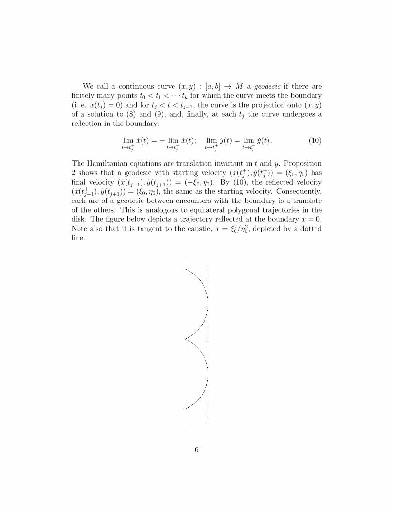
The Hamiltonian equations are translation invariant in t and y. Proposition2 shows that a geodesic with starting velocity (x(t+j ), y(t+j )) = (ξ0, η0) hasfinal velocity (x(t−j+1), y(t−j+1)) = (−ξ0, η0). By (10), the reflected velocity(x(t+j+1), y(t+j+1)) = (ξ0, η0), the same as the starting velocity. Consequently,each arc of a geodesic between encounters with the boundary is a translateof the others. This is analogous to equilateral polygonal trajectories in thedisk. The figure below depicts a trajectory reflected at the boundary x = 0.Note also that it is tangent to the caustic, x = ξ2

0/η20, depicted by a dotted

line.

6

Proposition 3. A closed geodesic with k = 1, 2, . . . reflections and windingnumber ` = ±1, ±2, . . . in the y variable, has length Lk,` > 0 determined bythe equations

Lk,`η2

0√1− η2

0

= 4k, Lk,`

(1

3η0 +

2

3η0

)= 2π` (11)

Proof. Proposition 2 shows that the length of a closed geodesic with k re-flections is kT , with T given as in the proposition. Hence, using ξ2

0 + η20 = 1,

Lk,` = kT = 4kξ0/η20 =⇒ Lk,`

η20√

1− η20

= 4k .

Moreover, if the winding number is `, then if y(t) is as in Proposition 2 withy(0) = 0,

ky(T ) = 2π` =⇒ k(4ξ0/η0 + (8/3)ξ30/η

30) = 2π`

Substitituting Lk,` = 4kξ0/η20 into the last equation, it can be written

Lk,`(η0 + (2/3)ξ20/η0) = 2π` ⇐⇒ Lk,`

(1

3η0 +

2

3η0

)= 2π`

The Friedlander length spectrum is defined by

LF = Lk,` : k ∈ N, ` ∈ Z− 0

where Lk,` solve the equations of Proposition 3 for some η0, −1 < η0 < 1.Note that if η0 is replaced by −η0, then ` is replaced by −` and Lk,−` =Lk,` > 0. Thus we may confine our attention to (k, `) ∈ N× N.

The implicit definition of Lk,` can be restated as follows. Let

H : R+ × R+ → R

be the homogeneous function of degree 1 that is equal to 1 on the curve

u→(π

2

u2

√1− u2

,

(u

3+

2

3u

))0 < u < 1. (12)

Then Lk,` = H(2πk, 2π`).

7

Proposition 4. The Friedlander length spectrum LF can be written

LF = H(2πN× 2πN) (13)

Furthermore,a) LF = LF ∪ 2πN.b) For each ` ∈ N, there is ε` > 0 such that (2π`, 2π`+ ε`) ∩ LF = ∅.c) LF ∩ 2πN = ∅

Proof. Because the curve (12) is the graph of a decreasing function, Lk,` <Lk+1,`. Furthermore, L1,` → ∞ as ` → ∞. Therefore, every sequence ofdistinct values of Lk,` tends to infinity unless ` remains bounded. It followsfrom this and the fact that the curve (12) is asymptotic to the horizontal lineof height 1 that all the limit points are given by

limk→∞

Lk,` = 2π` limk→∞

H(k/`, 1) = 2π`

The sequence Lk,` is increasing in k for fixed `, so (a) and (b) are established.Finally, to confirm (c), note that if 2πm = Lk,` for some (k, `), then theequations (11) imply that π is algebraic, a contradiction.

Proposition 4 (a) and (c) imply Theorem 1 (a).

2 Poisson summation formula with classical

symbols

The symbol class Sm(Rn) is the set of functions a ∈ C∞(Rn) satisfying

|∂αωa(ω)| ≤ Cα(1 + |ω|)m−α1−α2−···−αn , ω ∈ Rn (14)

for all multi-indices α = (α1, α2, . . . , αn) and some constants Cα. Smcl (Rn)consists of the symbols in Sm(Rn) with an asymptotic expansion, that is,there are homogeneous functions aj of degree m − j, smooth except at theorigin, and a cut-off function χN ∈ C∞(Rn) such that χN = 1 on |ω| ≥ CN ,and (

a−N∑j=0

aj

)χN ∈ Sm−N−1(R2) (15)

8

The function a0 is the principal symbol of a. Functions defined on a coneΓ ⊂ Rn belong to the symbol class Sm(Γ) (Smcl (Γ)) if they are restrictions ofsymbols in the class Sm(Rn) (Smcl (Rn)).

Let F be a real-valued symbol of first order, F ∈ S1cl(R2) with positive

principal symbol. Let T2 be the 2-torus, R2/2πZ2, and let P : C∞(T2) →C∞(T2) be the constant coefficient self-adjoint first order elliptic pseudodif-ferential operator given by

P (e2πi(mx+ny)) = F (m,n)e2πi(mx+ny)

The eigenvalues of P are F (m,n), (m,n) ∈ Z2, and hence its wave trace is

Z(t) =∑

(m,n)∈Z2

eitF (m,n) . (16)

Since the summands are smooth functions of t, the singularities of Z(t) de-pend only on the asymptotic behavior of F (m,n) as (m,n) → ∞. Forsimplicity we will assume that F = F1 on ξ2 +η2 ≥ 1/2, where F1 is homoge-neous of degree 1 and positive. (With small modifications the proof we willgive applies in general.)

To identify the length spectrum, consider the Hamiltonian flow on thecotangent bundle of T2 associated with the symbol, F1, defined by the ordi-nary differential equations

x = ∂ξF1, y = ∂ηF1, ξ = η = 0, (17)

Its periodic trajectories are curves of the form, (x, y)+t∇F1(ξ, η), 0 ≤ t ≤ T ,satisfying

T∇F1(ξ, η) = 2π(p, q) (18)

for some T > 0 and some (p, q) ∈ Z2. Let Tp,q be the set of T for which (18)has a solution for some (ξ, η) 6= (0, 0). (Note that ∇F1 is homogeneous ofdegree 0, so that we may as well assume ξ2 + η2 = 1.) The length spectrumis given by

L =⋃

(p,q)∈Z2

Tp,q

Note that because ∇F1 is nonzero, bounded, and continuous on ξ2 + η2 = 1,the length spectrum is closed and bounded away from 0. Our goal is to provethat the function Z(t) in (16) is C∞ in t > 0 on the complement of the lengthspectrum.

9

To do so we will apply the Poisson summation formula to the function,eitF (ξ,η). The Fourier transform of this function is∫

R2

ei(tF (ξ,η)−2π(xξ+yη)) dξdη

so by the Poisson summation formula,

Z(t) =∑

(p,q)∈Z2

Zp,q(t) (19)

where

Zp,q(t) =

∫R2

ei(tF (ξ,η)−2π(pξ+qη)) dξdη . (20)

We will first show that on the complement of the length spectrum theseindividual summands are C∞. If t0 > 0 and t0 /∈ L then there exists aninterval, t0−ε ≤ t ≤ t0+ε, such that for all |(ξ, η)| ≥ 1, either t∂ξF (ξ, η)−2πpor t∂ηF − 2πq is non-zero. Hence for t on this interval Zp,q(t) can be writtenas a sum

3∑r=1

∫R2

ei(tF−2π(pξ+q,n))ρr(ξ, η) dξdη (21)

where ρ1 and ρ2 are smooth homogeneous functions of degree zero on |(ξ, η)| ≥1 and the first of the functions above is non-zero on supp ρ1 and the secondnon-zero on supp ρ2. Finally ρ3 is supported in a compact neighborhood ofthe origin. The third integrand is compactly supported, and the correspond-ing integral converges along with all derivatives with respect to t, regardlessof the range of t. Let

a0(ξ, η, p, t) = i (t∂ξF − 2πp)−1 . (22)

Thenei(tF−2π(pξ+qη))ρ1 = a0∂ξ

(ei(tF−2π(pξ+qη))

)ρ1

hence by integration by parts the first summand of (21) can be written as∫R2

ei(tF−2π(pξ+qη))a1 dξdη

or inductively as ∫R2

ei(tF−2π(pξ+qη))aN dξdη

10

wherea1 = −∂ξ(a0ρ1); aN(ξ, η, p, t) = −∂ξ(a0aN−1) . (23)

Since a0 is a homogeneous function of degree zero in (ξ, η) outside a smallneighborhood of the origin, it follows by induction from (23) that aN is ahomogeneous function of degree −N , and hence

|aN(ξ, η, p, t)| ≤ CN(1 + |ξ|2 + |η|2)−N/2 (24)

uniformly on the interval −ε + t0 ≤ t ≤ ε + t0. Differentiation k times withrespect to t introduces the factor F k in the integrand, which is dominatedby |(ξ, η)|k; hence the integral converges. In all, the first of the summand in(21) is a C∞ function of t in the range specified. The proof for the term ρ2 issimilar, replacing a0 by b0 = i (t∂ηF − 2πq)−1, a1 by b1 = −∂η (b0ρ2) and aNby bN = −∂η (a0 bN−1) one concludes by the same argument that the secondof these summands is C∞ using integration by parts in η.

For |p| large, t∂F/∂ξ − 2πp is non-vanishing for all (ξ, η) and all t int0 − ε ≤ t ≤ t0 + ε, and integration by parts with respect to ξ yields

Zp,q(t) =

∫R2

ei(tF−2π(pξ+qη))aN dξdη, N = 1, 2, . . .

with a0 = 1 andaN = −∂ξ(a0aN−1)

The estimate (24) is replaced by

|aN(ξ, η, p, t)| ≤ CN(1 + |ξ|2 + |η|2)−N/2|p|−(N+1), N ≥ 1 (25)

Similarly, for |q| large, integration by parts with respect to η yields an analo-gous formula with better decay as q →∞. Hence if we break the sum

∑Zp,q

into subsums,∑Zp,q, |p| < |q|, and

∑Zp,q, |p| ≥ |q|, and make use of these

estimates we conclude that not only are the individual summands of (19)C∞ but that the sum itself is C∞ on the complement of the length spectrumL.

3 Non-classical symbols

Let Γ be a cone (sector with vertex at the origin) in R2.

11

Definition 1. A smooth function a : Γ→ C belongs to Σα,β(Γ) if there existsconstants Cj,k so that for all (ξ, η) ∈ Γ, the following upper bounds hold

∀j, k ≥ 0, |∂jξ∂kηa(ξ, η)| ≤ Cj,k(1 + |ξ|)α−j(1 + |η|)β−k .

A typical example is b(ξ)c(η) ∈ Σα,β(R2) if b ∈ Sα(R) and c ∈ Sβ(R).

Proposition 5. The following properties hold.a) S0(Γ) ⊂ Σ0,0(Γ).b) If a ∈ Σα,β(Γ) and b ∈ Σα′,β′(Γ), the product ab belongs to Σα+α′,β+β′(Γ).c) If a ∈ Σα,β(Γ) and a ≥ C(1+|ξ|)α(1+|η|)β with C > 0 in Γ (a is said to

be elliptic positive), then a−1 ∈ Σ−α,−β(Γ). Moreover, (a+ c)−1 ∈ Σ−α,−β(Γ)uniformly for all constants c ≥ 0.

To establish the symbol properties of the phase√λ(m,n) in the formula

(7) for the Friedlander wave trace ZF , we will need a well known asymptoticformula for the roots of the Airy function. (A proof is given in Appendix A;see also [AS] page 450.)

Proposition 6. There is a symbol τ ∈ S2/3cl (R+) such that τ(ξ) > 0 for all

ξ > 1/2,tm = τ(m), m = 1, 2, . . .

are the roots of Ai(−t) = 0, and the principal symbol of τ(ξ) is (3πξ/2)2/3

(ξ →∞).

DenoteF (ξ, η) = (η2 + η4/3τ(ξ))1/2

Then√λ(m,n) = F (m, |n|) and the sum (7) can be written

ZF (t) = 2∑

(m,n)∈N×N

eitF (m,n)

Let 0 < κ1 < κ2 < ∞. The first quadrant is covered by the union of threeoverlapping sectors

Γ1 = (ξ, η) : |ξ| < κ1η;Γ2 = (ξ, η) : (κ1/2)η < ξ < 2κ2ηΓ3 = (ξ, η) : κ2|η| < ξ

One can deduce easily from Proposition 6 the following.

12

Proposition 7. Let G(ξ, η) = F (ξ, η)− η. Thena) G ∈ Σ2/3,1/3(Γ1), and ∂ηG is positive, elliptic in Σ2/3,−2/3(Γ1).b) F ∈ S1

cl(Γ2) with principal symbol F0 given by

F0(ξ, η) =√η2 + (3πξ/2)2/3η4/3

c) F ∈ Σ1/3,2/3(Γ3), and ∂ξF is positive elliptic in Σ−2/3,2/3(Γ3).

4 Poisson summation formula with non-class-

ical symbols

We are now ready to finish the proof of Theorem 1. First, we divide the sumrepresenting ZF into three regions corresponding to different behaviors of thesymbol F (ξ, η). Let χj ∈ S0(R2) be supported in Γj and such that

3∑j=1

χj(ξ, η) = 1 for all ξ > 0, η > 0, ξ2 + η2 ≥ 1/4

Let ψ ∈ C∞(R) satisfy ψ(ξ) = 1 for all ξ ≥ 1 and ψ(ξ) = 0 for all ξ ≤ 1/2.Then

ZF (t) = 23∑j=1

Ij(t), Ij(t) =∑

(m,n)∈Z2

eitF (m,n)ψ(m)ψ(n)χj(m,n)

The method of Section 2 applies in the sector Γ2. The times t at whichsingularities can occur are the stationary points Tp,q of the phases of therepresentation using the Poisson summation formula, namely, solutions to

Tp,q∇F0(ξ, η) = 2π(p, q) (26)

Furthermore, on F0(ξ, η) = 1,

∇F0(ξ, η) =

(π

2

η2√1− η2

,1

3η +

2

3η−1

)Thus if (k, `) ∈ N × N, then Tk,` = Lk,`, exactly the points of the lengthspectrum LF . The set of Tp,q is

−LF ∪ 0 ∪ LF

13

(Evidently, T0,0 = 0 is a stationary point; there are no roots T0,q, q 6= 0 andno roots Tp,0, p 6= 0 of (26). The rest of the range (p, q) ∈ Z × Z is coveredby the symmetries Tk,−` = Tk,` and T−k,−` = −Tk,`.)

The restriction to Γ2 gives a further limitation on the set of stationarypoints. Define a smaller collection of stationary points by

LF (M) = Lk,` : (k, `) ∈ N2, 1 ≤ k ≤M`

LF (M) is a closed, discrete set in R. For M sufficiently large depending onκ1, all the stationary values that occur in the the range ξ ≥ κ1|η|/2 are inLF (M). Because LF (M) has no limit points, and the symbol of the phasehas classical behavior in Γ2, the method of Section 2 applies and yields thefollowing.

Proposition 8. For M sufficiently large depending on κ1, I2 is smooth inthe complement of

LF (M) ∪ (−LF (M)) ∪ 0

In particular, for any ` ∈ N and any κ1 > 0 there is ε > 0 such that

I2 ∈ C∞((2π`− ε, 2π`+ ε))

All the remaining singularities in LF − LF (M) are accounted for in Γ1,associated with I1. The main issue is the limit points at t = 2π`. Ourtheorem in Γ1 is stated in sufficient generality to apply as well to the case ofthe disk.

Theorem 2. Let ψ(ξ) be a classical symbol of degree 0 in one variable sup-ported in ξ ≥ 0 and let χ(ξ, η) be a classical symbol of degree 0 supported ina cone Γ1 given by |ξ| ≤ κ1η. Suppose that the distribution Z is defined by

Z(t) =∑

(m,n)∈Z2

ψ(m)χ(m,n)eit(n+G(m,n)) ,

where G belongs to Σ2/3,1/3, with ∂ηG > 0 is positive elliptic in Σ2/3,−2/3 onthe support of ψ(m)χ(m,n). For any T > 0 there exist ε > 0 and κ1 > 0sufficiently small depending on T and the constant in the symbol upper boundon ∂ηG such thata) if T = 2π`, ` ∈ N, then Z is smooth on [T, T + ε);b) if T /∈ 2πN, then Z is smooth on (T − ε, T + ε).

14

Proof. In the proof of part (a) we will assume for simplicity that ` = 1. Theother cases are similar. Let F (ξ, η) = η + G(ξ, η). The Poisson summationformula says

Z(t) =∑

(p,q)∈Z2

Zp,q(t)

with

Zp,q(t) =

∫R2

ψ(ξ)χ(ξ, η)ei(tF (ξ,η)−2π(pξ+qη))dξdη ,

Denote Q = i(tF (ξ, η)− 2π(pξ+ qη)) and define two differential operators inorder to integrate by parts as follows.

Af = eitF (ξ,η) i

2π∂ξ(e

−itF (ξ,η)f) =i

2π∂ξf +

t

2π(∂ξF )f .

Bf =1

i(t∂ηF (ξ, η)− 2πq)∂ηf

Then1

pA(eQ) = B(eQ) = eQ.

Let us start with the most singular case q = 1. Because G ∈ Σ2/3,1/3, wehave

∂ξF = ∂ξG ∈ Σ−1/3,1/3, ∂ηG ∈ Σ2/3,−2/3 .

The main point is that by Proposition 5,

ψ(ξ)χ(ξ, η)

t∂ηF − 2π=

ψ(ξ)χ(ξ, η)

t− 2π + ∂ηG∈ Σ−2/3,2/3

uniformly in t > 2π. Let A′ and B′ denote the adjoint operators to A andB. Then Proposition 5 also implies that

A′(Σα,β) ⊂ Σα−1/3,β+1/3; B′(Σα,β) ⊂ ∂ηΣα−2/3,β+2/3 ⊂ Σα−2/3,β−1/3

with constants in the estimates independent of p.

Zp,1(t) = p−M∫eQ(A′)M(B′)N(ψ(ξ)χ(ξ, η))dξdη .

Since ψ(ξ)χ(ξ, η) ∈ Σ0,0, the symbol p−M(A′)M(B′)N(ψ(ξ)χ(ξ, η)) belongsto Σ−(M+2N)/3,(M−N)/3 with constants O(|p|−M). Note that symbols in Σα,β

supported in the cone 0 ≤ ξ ≤ η are integrable if max(α, 0) + β < −1.

15

Therefore it suffices to take N ≥M + 5 to get a convergent integral. In casep = 0, take M = 0 and N large. Otherwise, take M ≥ 2 so that the sumover p converges. So far we have shown that that sum over (p, 1) is bounded.To prove smoothness in t, differentiate k times. This yields an extra factorF k ∈ Σ2k/3,k in the integrand. Therefore,∑

p∈Z

(d/dt)kZp,1(t)

is represented by sum of integrals of symbols Σ2k/3−M/3−2N/3,k+M/3−N/3 withconstants O(|p|−M). The integrals converge for N large, for instance N ≥M + 3k + 10. Again, take M = 0 when p = 0 and M ≥ 2 when p 6= 0.

Next, consider q 6= 1. The same estimates as before hold for A′. Recallthat we may assume that χ is zero on a fixed compact subset. Provided t isclose enough to 2π, and κ1 sufficiently small, and |ξ| + |η| sufficiently largeon the support of χ, we have

|∂ηG| ≤ C((1 + |ξ|)/(1 + |η|))2/3 ≤ Cκ1 << 1

and hence |t∂ηF − 2πq| ∼ |q − 1| and

ψ(ξ)χ(ξ, η)/(t∂ηF − 2πq) ∈ Σ0,0, with constants O(1/|q − 1|)

Hence,B′ : Σα,β → Σα,β−1

with constants O(1/|q−1|). So the symbol p−M(A′)M(B′)N(ψ(ξ)χ(ξ, η)) be-longs to Σ−M/3,−N with constants O(|p|−M |q−1|−N). The integral convergesprovided N ≥ 2. When p = 0, take M = 0; when p 6= 0 take M ≥ 2.Then the sum over (p, q), with q 6= 1 also converges. Lastly, if we apply(d/dt)k, we obtain integrands that belong to Σ2k/3−M/3,k−N with constantsO(|p|−M |q − 1|−N), so the symbols are integrable if N ≥ 5k/3 + 2. To sumthe series, for p 6= 0, q 6= 1, let M ≥ 2. For p = 0, q 6= 1, use M = 0. Thisconcludes the proof of part (a) of Theorem 2.

For part (b), once again for any δ > 0 we can choose κ1 > 0 sufficientlysmall that on the support of χ (where |ξ|+ |η| is sufficiently large)

|∂ηG| ≤ C((1 + |ξ|/(1 + |η|)2/3 ≤ Cκ2/31 < δ

16

Let q0 be the integer such that |T − 2πq0| is smallest, and choose both δ > 0and ε > 0 less than |T −2πq0|/4. Then for t ∈ (T −ε, T +ε), |t∂ηF −2πq0| ≥|T − 2πq0|/4 on the support of χ. Hence,

ψ(ξ)χ(ξ, η)/(t∂ηF − 2πq) ∈ Σ0,0, with constants O(1/(1 + |q − q0|))

and the rest of the proof proceeds as in the case q 6= 1 above. This concludesthe proof of Theorem 2.

The next proposition will take care the integral I3.

Proposition 9. Let ψ ∈ C∞(R) satisfy ψ(η) = 1 for η sufficiently large andψ(η) = 0 for η ≤ 0. Suppose that where F belongs to Σ1/3,2/3 and ∂ξF ispositive elliptic in Σ−2/3,2/3 on the cone 0 < η < ξ. For each T < ∞ thereexists κ2 such that if χ(ξ, η) is a classical symbol of degree 0 supported in acone Γ given by ξ > κ2|η|, then the distribution

Z(t) =∑

(m,n)∈Z2

ψ(n)χ(m,n)eitF (m,n) ,

satisfies Z ∈ C∞((0, T )).

Proof. As usual, the Poisson summation formula implies

Z(t) =∑

(p,q)∈Z2

Zp,q(t)

with

Zp,q(t) =

∫R2

ψ(η)χ(ξ, η)ei(tF (ξ,η)−2π(pξ+qη))dξdη ,

Denote Q = i(tF (ξ, η)− 2π(pξ + qη)) .Case 1. p = 0. Then Q = i(tF − 2πqη) and

Z0,q(t) =

∫ ∫eQψ(η)χ(ξ, η) dξdη = −

∫ ∫eQ∂ξ(χ/∂ξQ)ψ(η) dξdη

= · · · =∫ ∫

eQaM(ξ, η)ψ(η) dξdη

with a0 = χ, aM+1 = −∂ξ(aM/∂ξQ). Since ∂ξF is positive elliptic inΣ−2/3,2/3(Γ),

1/∂ξQ = 1/it∂ξF

17

belongs to Σ2/3,−2/3 with support on Γ and bounds depending on 1/t. Byinduction, aM ∈ Σ−M/3,−2M/3 with support in Γ3. Thus Z0,q is represented bya convergent integral. Moreover, if q = 0, we may differentiate k times withrespect to t to obtain an integrand dominated by |aMF k| which is integrableif k < M/3− 2. For q 6= 0, use

e2πiqη =1

2πiq∂ηe

2πiqη

to integrate by parts N times to obtain

(d/dt)jZ0,q(t) =±1

(2πiq)N

∫ ∫eQ∂Nη

[(iF )jeitFψ(η)aM(ξ, η)

]dξdη

The integrand is majorized by (1 + |ξ|)j+(N−M)/3 which is convergent in Γfor sufficiently large M depending on j and N . (Note that because χ issupported in ξ < |η|, ψ′(η)χ(ξ, η) has compact support, and every term inwhich a derivative falls on ψ is convergent.) The factor 1/qN makes the sumover q convergent as well.

Case 2. p 6= 0. We use the same integration by parts as in Case 1. Notethat the set of (m,n) ∈ Z2 where ψ(n)χ(m,n) > 0 and m < ξ0 is finite. Anyfinite sum of exponentials is smooth in t, so we may assume without loss ofgenerality that χ(ξ, η) is supported on ξ > ξ0 for some large ξ0. It followsthat

∂ξF (ξ, η) ≤ Cξ−2/3η2/3

on the support of ψ(η)χ(ξ, η). Furthermore, if κ2 is sufficiently large, de-pending on T ,

0 ≤ t∂ξF ≤ CTκ−2/32 ≤ π, for all 0 ≤ t ≤ T

Thusχ/∂ξQ = 1/i(t∂ξF − 2πp) ∈ Σ0,0(Γ)

with bounds O(1/|p|). By induction,

aM ∈ Σ−M,0

with bounds O(1/|p|M). The rest of the proof proceeds as in Case 1. Ifq = 0, then no more integrations by parts are needed. If q 6= 0, then one usesintegration by parts in η as in Case 1 to introduce a factor |q|−N so as to beable to sum in both p and q.

18

Finally, we assemble these ingredients to prove Theorem 1. Part (a) wasalready proved at the end of Section 1. For part(b), choose T /∈ LF ∪(−LF )∪0, and choose ε so that

[T − ε, T + ε] ∩ (LF ∪ (−LF ) ∪ 0) = ∅

Choose κ1 sufficiently small depending on the symbol bounds and the dis-tance from [T − ε, T + ε] to 2πZ and κ2 sufficiently large depending on thesize of T , we may apply Theorem 2 (b), Proposition 8 and Proposition 9,respectively, to I1, I2 and I3 to obtain smoothness in (T − ε, T + ε). Notethat Proposition 7 implies that the correponding phases satisfy the appro-priate symbol estimates. For part (c), apply Theorem 2 (a) to I1, to obtainsmoothness in [2π`, 2π`+ ε). By Propositions 8 and 9 I2 and I3 are smoothnear 2π` on both sides. This concludes the proof of Theorem 1.

5 Action variables

The classical mechanical system associated to the Friedlander model has twocommuting conserved quantities,

H(x, y, ξ, η) =√ξ2 + (1 + x)η2; J(x, y, ξ, η) = η.

In this section we will show how the action variables associated to this systemdetermine the first order asymptotics of the eigenvalues and eigenfunctionsof the Friedlander operator L. (See Appendix B for the general frameworkof this calculation.)

Let H0 and J0 be real numbers satisfying 0 < |J0| < H0. The Lagrangiansubmanifold

H = H0, J = J0 (27)

is a torus foliated by trajectories with initial velocity (ξ0, η0) on x = 0, withξ0 > 0, ξ2

0 + η20 = H0 and J0 = η0. These trajectories are tangent to the

caustic

x =ξ2

0

η20

=H2

0 − J20

J20

,

depicted as a dotted line in the figure below and in Section 1.Fix H = 1, so that ξ2

0 +η20 = 1. Denote by γ(t) = (x(t), y(t), ξ(t), η(t)) the

trajectory given by Proposition 2 on the interval −T/2 ≤ t ≤ T/2. Define byγ1 the loop (whose projection onto R+ × S1 is pictured in bold in the figure

19

below) that follows γ on its two curved portions and then the segment of thecaustic x = ξ2

0/η20, with ξ = 0, η = η0 (oriented by y < 0) going from γ(T/2)

to γ(−T/2).

Define by γ2 the loop that follows the caustic x = ξ20/η

20, 0 ≤ y ≤ 2π,

ξ = 0, and η = η0, with orientation y > 0.The loops γ1 and γ2 are a basis for the homology of the torus H = 1,

J = η0, and the action coordinates are defined by

I1 =

∫γ1

ξ dx+ η dy, I2 =

∫γ2

ξ dx+ η dy.

20

Since η(t) = η0 is constant, T = 4ξ0/η20, and H = H0 = ξ2

0 + η20, we have

I1 =

∫γ1

ξ dx =

∫γ

ξ dx

= 2

∫ T/2

0

(ξ0 − η20t/2)2 dt

=4ξ3

0

3η20

=4

3(H2

0 − η20)3/2η−2

0

Moreover,

I2 =

∫γ2

ξ dx+ η dy =

∫γ2

η dy = 2πη0

More generally, by homogeneity,

I1 =4

3(H2 − J2)3/2J−2; I2 = 2πJ.

Thus H and J can be written as functions of the action variables,

H2 = J2 +

(3

4I1J

2

)2/3

=I2

2

4π2+

(3I1I

22

16π2

)2/3

; J =I2

2π.

Define Λ(m,n) as the values of H2 when the action variables belong to theinteger lattice (I1, I2) = 2π(m,n), (m,n) ∈ Z2. (Since I1 > 0, we consideronly m > 0.) Then

Λ(m,n) = n2 + (3π/2)2/3m2/3n4/3.

The Bohr-Sommerfeld energy levels of H are defined as the values of H onthe lattice, namely

√Λ(m,n).

Proposition 10. In any sector of the form 0 < c1 ≤ |n|/m ≤ c2, theeigenvalues λ(m,n) of the Friedlander operator satisfy√

λ(m,n) =√

Λ(m,n) +O(1), (m,n)→∞

The proposition is an immediate consequence of the formula for L(m,n)and the fact that

λ(m,n) = n2 + n4/3τ(m),

21

with τ(m) = (3πm/2)2/3 +O(1), m = 1, 2, . . . (see Proposition 6).Next, we show that the phases of the eigenfunctions are equal, asymptot-

ically, to the generating function of the canonical relation of the Lagrangiansubmanifold (27). Indeed, if ρ(x, y) is the generating function, then by defi-nition, the Lagrangian is the graph of (x, y) 7→ (ρx, ρy):

ρ2x + (1 + x)ρ2

y = H20 ; ρy = J0 .

Thus,

ρx = ±√H2

0 − J20 − xJ2

0 ; 0 ≤ x ≤ H20 − J2

0

J20

,

and

ρ(x, y) = ±2

3

(H20 − J2

0 − xJ20 )3/2

J20

+ J0y

Notice that the upper limit of the range of x is exactly the caustic

x =H2

0 − J20

J20

,

so that the graph over this interval in x (and all y) covers the whole La-grangian submanifold.

Now let the submanifold be given by (I1, I2) = 2π(m,n). Then

H20 = n2 +

(3

2πmn2

)3/2

; J0 = n,

and we have two generating functions

ρ±(x, y) = ±2

3

((3π

2m

)2/3

− n2/3x

)3/2

+ ny.

To compare this with the phase of ϕm,n, recall that for tm > n2/3x,

ϕm,n(x, y) = Ai(n2/3x− tm)einy

∼ 1

2π−1/2|n2/3x− tm|−1/4 sin

(2

3(tm − n2/3x)3/2 + π/4

)einy .

(See Proposition 1 and Appendix A.) Thus ϕm,n is a sum of two terms withphases

±[

2

3

(tm − n2/3x

)3/2+ π/4

]− π/2 + ny = ρ±(x, y) +O(1),

22

as (m,n) → ∞ in sectors of the form 0 < c1 < |n|/m < c2 (since tm =(3πm/2)2/3(1 +O(1/m))).

Appendix A: Airy functions

An Airy function is a solution y(t) of the differential equation y′′ = ty. Theclassical properties of Airy functions are treated in [AS], Section 10.4 and[H], Section 7.6, and reviewed briefly here.

The Airy function (or Airy integral), denoted Ai, was introduced in 1838by G.B. Airy in the remarkable paper [Ai] in order to describe the intensityof the light near a caustic. This allowed him to propose a good theory forthe rainbow. He defined the function Ai by the oscillatory integral

Ai(s) =1

2π

∫ ∞−∞

ei(sx+x3/3) dx (28)

In other words, Ai is the inverse Fourier transform of x 7→ eix3/3.

The Airy function Ai(t) is positive for t ≥ 0 and decays exponentially ast → +∞; it is oscillating for t < 0 with an expansion, given by the methodof stationary phase, of the form

Ai(t) = π−1/2|t|−1/4[sin(ζ +

π

4

)+ Re (eiζα(ζ))

], t < 0,

with ζ = 23|t|3/2 and α a classical symbol of order −1. Differentiating, we

findAi′(t) = −π−

12 |t|1/4

[cos(ζ +

π

4

)+ Re (eiζβ(ζ))

], t < 0,

with β a classical symbol of order −1.The function Ai has infinitely many real negative zeros

· · · < −tm < · · · < −t1 < 0 .

To derive the asymptotic formula for tm, denote

f(s) = is1/3Ai(−s2/3)− Ai′(−s2/3), s > 0.

The foregoing asymptotic expansions can be written

f(s) =1√πs1/6ei(2s/3+π/4)+c(s),

23

where c is a complex valued classical symbol of order −1. Define

θ(s) = 2s/3 + π/4 + Im c(s) = arg f(s),

Im f(s) > 0 for all 0 < s < t3/21 , and specify the branch of θ by 0 < θ(s) < π

in that range. Thus θ is a classical symbol of order 1 with principal part2s/3 as s→∞, and

tan θ(s) = −s1/3Ai(−s2/3)

Ai′(−s2/3), s > 0. (29)

Proposition 11. Let θ be as above. Then θ′(s) > 0 for all s > 1/4, andthere is an absolute constant c1 < 1 such that

τ(ξ) = [θ−1(πξ)]2/3 > 0, for ξ ≥ c1,

is well defined; τ ∈ S2/3cl (R+) with principal term (3πξ/2)2/3. Finally,

tm = τ(m), m = 1, 2, . . . ,

where 0 > −t1 > −t2 > · · · are the zeros of Ai.

Proof.

θ′(s) = (1/3|f ′|2)[2s2/3a2 + 2b2− s−2/3ab], a = Ai(−s2/3), b = Ai′(−s2/3).

Therefore, θ′(s) > 0 for s > 1/4. Because θ is increasing, the zeros of Ai aregiven by

θ(t3/2m ) = mπ, m = 1, 2, . . .

Let θ(1/4) = θ0. 0 < θ0 < θ(t3/21 ) = π because t

3/21 ≈ (2.33)3/2 > 1/4.

The inverse function σ of θ is a classical symbol of order 1 on [θ0,∞). Thenτ(ξ) = σ(πξ)2/3 is defined for all ξ ≥ θ0/π and satisfies all the properties ofthe proposition.

Now we turn to proof of Proposition 1 describing the spectrum of theFriedlander operator L. Begin by noting that if L is restricted to functionsf(x) of x alone, it becomes

Lf(x) = −f ′′(x),

24

which has completely continuous spectrum on L2([0,∞)). Next, consider ϕin the orthogonal complement,

ϕ ∈ L2(M) :

∫R/2πZ

ϕ(x, y) dy = 0

By separation of variables, the eigenfunctions are of the form f(x)einy, wheren is a non-zero integer, and f satisfies

Lnf := (−∂2x + n2(1 + x))f = −λf (30)

For n 6= 0, the operator Ln acting on functions satisfying f(0) = 0 is self-adjoint and has compact resolvent, so a complete system of eigenfunctions isobtained by solving (30) for λ and f such that f(0) = 0 and f ∈ L2([0,∞)).Making the change of variables

f(x) = A(n2/3x− t),

equation (30) becomes

n4/3(−A′′(s) + sA(s)) = (λ− n4/3t− n2)A(s) .

Choose t so that λ = n2 + n4/3t, then the equation is the Airy equation

− A′′(s) + sA(s) = 0 (31)

Since f is in L2([0,∞)), the same is true of A. Up to a constant multi-ple, there is a unique such function A, the Airy function Ai. The Dirichletcondition f(0) = 0 implies Ai(−t) = 0, and the roots of this equation are0 < t1 < t2 < · · · . Hence the formulas in the proposition for the eigenfunc-tions and eigenvalues are confirmed.

Appendix B: Semiclassical properties of eigen-

functions and eigenvalues for completely inte-

grable systems

Let X be an n-dimensional manifold and P1, . . . , Pn be commuting self-adjoint zero order semiclassical pseudodifferential operators with leadingsymbols p1, . . . , pn. In Section 5 we considered the example X = R+ × S1,

P1 = 2(∂2x + (1 + x)∂2

y); P2 = i∂y.

25

(These operators are of order zero with respect to ∂x, ∂y and multiplicationby .)

We seek the joint eigenfunctions ϕ(x), x ∈ X, of Pj in the form

ϕ(x) = a(x, h)eiρ(x)/h, a(x, h) = a0(x) + ha1(x) + h2a2(x) + · · · , (32)

solving asymptotically as → 0

Pjϕ = λj(h)ϕ, j = 1, . . . , n, λj(h) = λj(0) + hλj,1 + h2λj,2 + · · · .

Let Λρ be the graph of dρ in T ∗X. Λρ is a Lagrangian submanifoldand determines ρ up to an additive constant; ρ is known as the generatingfunction of Λρ. Setting = 0, one finds the eikonal equation, the first of theheirarchy of equations for a, ρ, and λj(h):

pj|Λρ = λj(0) . (33)

Let us confine ourselves to the sequence = 1/N for integers N → ∞.Then (32) defines ϕ provided ρ is well-defined modulo 2πZ. To see whatthis entails, denote by κ the projection, Λρ → X, and by ι the inclusion,Λρ → T ∗X, and denote

α =n∑j=1

ξjdxj ,

the canonical 1-form on T ∗X. The fact that Λρ is the graph of dϕ implies

dκ∗ρ = ι∗α . (34)

If (λ1(0), . . . , λn(0)) is a regular value of (p1, . . . , pn) and Λρ is compact, thenΛρ is a torus of dimension n. Thus if γ1, . . . , γn is a basis of the first homologygroup of Λρ, then (34) implies

Proposition 12. ρ is well-defined modulo 2πZ if and only if

Ij :=

∫γj

α ∈ 2πZ, j = 1, 2, . . . , n.

The functions Ij are known as action coordinates on T ∗X. Let m ∈ Zn.In the generic case in which

(I1, . . . , In) = 2πm

26

defines an n-dimensional Lagrangian torus in T ∗X, the torus is known as aBohr-Sommerfeld surface, and we will denote it by S(m).

Proposition 12 says that the generating function ρm of S(m) is well-defined modulo 2πZ. Thus one can follow the ansatz (32) to seek a jointeigenfunction ϕ whose phase function ρ equals ρm to first order as → 0and whose eigenvalue λj with respect Pj is given to first order by pj evaluatedon S(m) as in (33). Under suitable further hypotheses, all but finitely manyjoint eigenfunctions are obtained in this way. Typically, ϕ and S(m) existfor a cone of values of m ∈ Zn (see [CdV1]).

References

[AS] M. Abramowitz and I. Stegun, Handbook of Mathematical Functions.National Bureau of Standards Applied Mathematics Series 55, 10th edi-tion (1972).

[Ai] G.B. Airy, On the Intensity of Light in the neighborhood of a Caustic.Transactions of the Cambridge Philosophical Society 6:379–402 (1838).

[AM] K. G. Andersson and R. B. Melrose, The propagation of singularitiesalong gliding rays, Invent. Math. 41 (1977) no. 3, 97–232.

[Ch] J. Chazarain, Formule de Poisson pour les varietes riemanniennes. In-ventiones Math. 24: 65–82 (1974).

[CdV0] Y. Colin de Verdiere, Spectre du laplacien et longueurs desgeodesiques periodiques. Compositio Math. 27:159–184 (1973).

[CdV1] Y. Colin de Verdiere, Spectre joint d’operateurs pseudo-differentielsqui commutent II. Le cas integrable. Math. Zeitschrift 171:51–73 (1980).

[CGJ] Y. Colin de Verdiere, V. Guillemin and D. Jerison, Singularities of thewave trace near cluster points of the length spectrum. arXiv:1101.0099v1(2011).

[DG] H. Duistermaat and V. Guillemin, The spectrum of positive ellipticoperators and periodic geodesics. Inventiones Math. 29:39–79 (1975).

27

[F] F.G. Friedlander, The wave front set of the solution of a simple initialboundary value problem with glancing rays. Math. Proc. CambridgePhil. Soc. 79:145–159 (1976).

[GM] V. Guillemin and R. Melrose, The Poisson summation formula formanifolds with boundary. Advances Math. 32:204–232 (1979).

[H] L. Hormander, The Analysis of Partial Differential Operators I, 2nd ed.,Springer Verlag (1990).

28