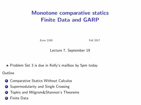
Monotone comparative staticsFinite Data and GARP

Econ 2100 Fall 2017

Lecture 7, September 19

Problem Set 3 is due in Kelly’s mailbox by 5pm today

Outline

1 Comparative Statics Without Calculus2 Supermodularity and Single Crossing3 Topkis and Milgrom&Shannon’s Theorems4 Finite Data

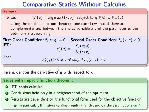
Comparative Statics Without CalculusRemark

Let x∗(q) = argmax f (x , q), subject to q ∈ Θ, x ∈ S(q)

Using the implicit function theorem, one can show that if there arecomplementarities between the choice variable x and the parameter q, theoptimum increases in q.

First Order Condition: fx (x ; q) = 0. Second Order Condition: fxx (x ; q) < 0.IFT:

x∗q (q) = − fxq(x ; q)

fxx (x ; q).

Thenx∗q (q) ≥ 0 if and only if fxq(x ; q) ≥ 0

Here g· denotes the derivative of g with respect to ·.

Issues with implicit function theorem:1 IFT needs calculus.2 Conclusions hold only in a neighborhood of the optimum.3 Results are dependent on the functional form used for the objective function.

1 In particular, IFT gives cardinal results that depend on the assumptions on f .

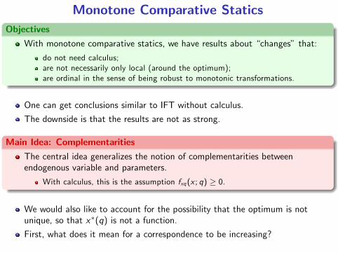
Monotone Comparative StaticsObjectives

With monotone comparative statics, we have results about “changes” that:

do not need calculus;are not necessarily only local (around the optimum);are ordinal in the sense of being robust to monotonic transformations.

One can get conclusions similar to IFT without calculus.

The downside is that the results are not as strong.

Main Idea: ComplementaritiesThe central idea generalizes the notion of complementarities betweenendogenous variable and parameters.

With calculus, this is the assumption fxq(x ; q) ≥ 0.

We would also like to account for the possibility that the optimum is notunique, so that x∗(q) is not a function.

First, what does it mean for a correspondence to be increasing?

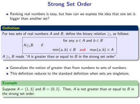
Strong Set Order

Ranking real numbers is easy, but how can we express the idea that one set isbigger than another set?

DefinitionFor two sets of real numbers A and B, define the binary relation ≥s as follows:

A≥sB iffor any a ∈ A and b ∈ B

min{a, b} ∈ B and max{a, b} ∈ A

A ≥s B reads “A is greater than or equal to B in the strong set order”.

Generalizes the notion of greater than from numbers to sets of numbers.

This definition reduces to the standard definition when sets are singletons.

Example

Suppose A = {1, 3} and B = {0, 2}. Then, A is not greater than or equal to B inthe strong set order.

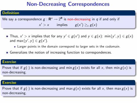
Non-Decreasing CorrespondencesDefinition

We say a correspondence g : Rn → 2R is non-decreasing in q if and only if

x ′ > x implies g(x ′) ≥s g(x)

Thus, x ′ > x implies that for any y ′ ∈ g(x ′) and y ∈ g(x): min{y ′, y} ∈ g(x)and max{y ′, y} ∈ g(x ′).

Larger points in the domain correspond to larger sets in the codomain.

Generalizes the notion of increasing function to correspondences.

Exercise

Prove that if g(·) is non-decreasing and min g(x) exists for all x , then min g(x) isnon-decreasing.

Exercise

Prove that if g(·) is non-decreasing and max g(x) exists for all x , then max g(x) isnon-decreasing.

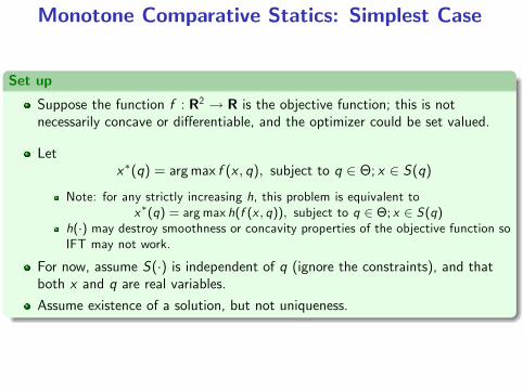
Monotone Comparative Statics: Simplest Case

Set up

Suppose the function f : R2 → R is the objective function; this is notnecessarily concave or differentiable, and the optimizer could be set valued.

Letx∗(q) = argmax f (x , q), subject to q ∈ Θ; x ∈ S(q)

Note: for any strictly increasing h, this problem is equivalent tox∗(q) = arg max h(f (x , q)), subject to q ∈ Θ; x ∈ S(q)

h(·) may destroy smoothness or concavity properties of the objective function soIFT may not work.

For now, assume S(·) is independent of q (ignore the constraints), and thatboth x and q are real variables.

Assume existence of a solution, but not uniqueness.

Supermodularity

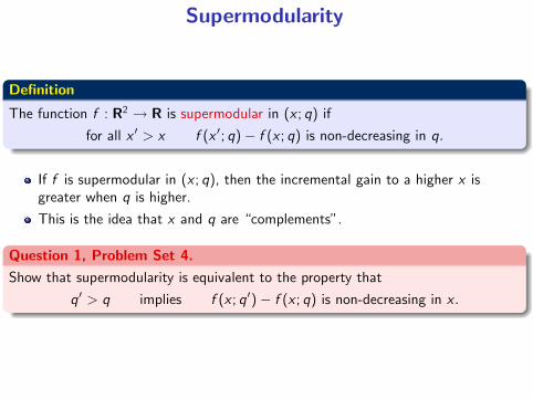
Definition

The function f : R2 → R is supermodular in (x ; q) if

for all x ′ > x f (x ′; q)− f (x ; q) is non-decreasing in q.

If f is supermodular in (x ; q), then the incremental gain to a higher x isgreater when q is higher.

This is the idea that x and q are “complements”.

Question 1, Problem Set 4.Show that supermodularity is equivalent to the property that

q′ > q implies f (x ; q′)− f (x ; q) is non-decreasing in x .

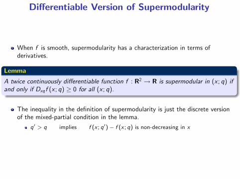
Differentiable Version of Supermodularity

When f is smooth, supermodularity has a characterization in terms ofderivatives.

Lemma

A twice continuously differentiable function f : R2 → R is supermodular in (x ; q) ifand only if Dxq f (x ; q) ≥ 0 for all (x ; q).

The inequality in the definition of supermodularity is just the discrete versionof the mixed-partial condition in the lemma.

q′ > q implies f (x ; q′)− f (x ; q) is non-decreasing in x

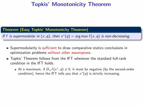
Topkis’Monotonicity TheoremTheorem (Easy Topkis’Monotonicity Theorem)

If f is supermodular in (x ; q), then x∗(q) = argmax f (x , q) is non-decreasing.

Proof.

Let q′ > q and take x ∈ x∗(q) and x ′ ∈ x∗(q′). Show that x∗(q′) ≥s x∗(q).

First show that max{x , x ′} ∈ x∗(q′)x ∈ x∗(q) implies f (x ; q)− f (min{x , x ′}; q) ≥ 0.x ∈ x∗(q) also implies that f (max{x , x ′}; q)− f (x ′; q) ≥ 0

verify these by checking two cases, x > x ′ and x ′ > x .

By supermodularity, f (max{x , x ′}; q′)− f (x ′; q′) ≥ 0,Hence max{x , x ′} ∈ x∗(q′).

Now show that min{x , x ′} ∈ x∗(q)

max{x , x ′} ∈ x∗(q′) implies that f (x ′; q′)− f (max{x , x ′}, q) ≥ 0,or equivalently f (max{x , x ′}, q)− f (x ′; q′) ≤ 0.

max{x , x ′} ∈ x∗(q′) also implies that f (max{x , x ′}; q′)− f (x ′; q′) ≥ 0,which by supermodularity implies f (x ; q)− f (min{x , x ′}; q) ≤ 0Hence min{x , x ′} ∈ x∗(q).

Topkis’Monotonicity Theorem

Theorem (Easy Topkis’Monotonicity Theorem)

If f is supermodular in (x ; q), then x∗(q) = argmax f (x , q) is non-decreasing.

Supermodularity is suffi cient to draw comparative statics conclusions inoptimization problems without other assumptons.

Topkis’Theorem follows from the IFT whenever the standard full-rankcondition in the IFT holds.

At a maximum, if Dxx f (x∗, q) 6= 0, it must be negative (by the second-ordercondition), hence the IFT tells you that x∗(q) is strictly increasing.

Example

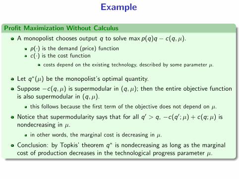
Profit Maximization Without Calculus

A monopolist chooses output q to solve max p(q)q − c(q, µ).

p(·) is the demand (price) functionc(·) is the cost function

costs depend on the existing technology, described by some parameter µ.

Let q∗(µ) be the monopolist’s optimal quantity.

Suppose −c(q, µ) is supermodular in (q, µ); then the entire objective functionis also supermodular in (q, µ).

this follows because the first term of the objective does not depend on µ.

Notice that supermodularity says that for all q′ > q, −c(q′;µ) + c(q;µ) isnondecreasing in µ.

in other words, the marginal cost is decreasing in µ.

Conclusion: by Topkis’theorem q∗ is nondecreasing as long as the marginalcost of production decreases in the technological progress parameter µ.

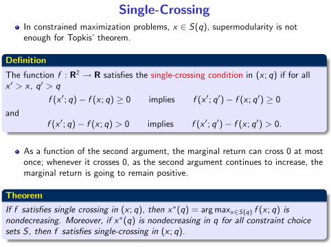
Single-CrossingIn constrained maximization problems, x ∈ S(q), supermodularity is notenough for Topkis’theorem.

Definition

The function f : R2 → R satisfies the single-crossing condition in (x ; q) if for allx ′ > x , q′ > q

f (x ′; q)− f (x ; q) ≥ 0 implies f (x ′; q′)− f (x ; q′) ≥ 0and

f (x ′; q)− f (x ; q) > 0 implies f (x ′; q′)− f (x ; q′) > 0.

As a function of the second argument, the marginal return can cross 0 at mostonce; whenever it crosses 0, as the second argument continues to increase, themarginal return is going to remain positive.

Theorem

If f satisfies single crossing in (x ; q), then x∗(q) = argmaxx∈S(q) f (x ; q) isnondecreasing. Moreover, if x∗(q) is nondecreasing in q for all constraint choicesets S, then f satisfies single-crossing in (x ; q).

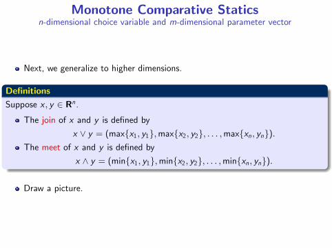
Monotone Comparative Staticsn-dimensional choice variable and m-dimensional parameter vector

Next, we generalize to higher dimensions.

DefinitionsSuppose x , y ∈ Rn .

The join of x and y is defined by

x ∨ y = (max{x1, y1},max{x2, y2}, . . . ,max{xn , yn}).The meet of x and y is defined by

x ∧ y = (min{x1, y1},min{x2, y2}, . . . ,min{xn , yn}).

Draw a picture.

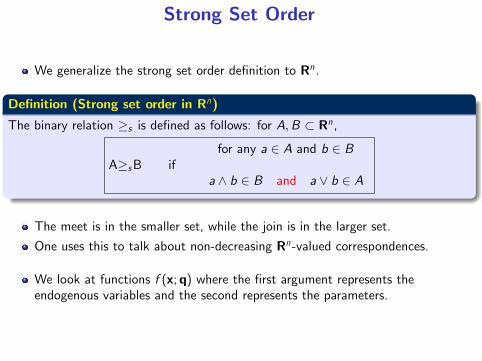
Strong Set Order

We generalize the strong set order definition to Rn .

Definition (Strong set order in Rn)

The binary relation ≥s is defined as follows: for A,B ⊂ Rn ,

A≥sB iffor any a ∈ A and b ∈ B

a ∧ b ∈ B and a ∨ b ∈ A

The meet is in the smaller set, while the join is in the larger set.

One uses this to talk about non-decreasing Rn-valued correspondences.

We look at functions f (x;q) where the first argument represents theendogenous variables and the second represents the parameters.

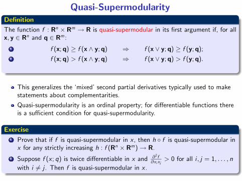
Quasi-SupermodularityDefinitionThe function f : Rn × Rm → R is quasi-supermodular in its first argument if, for allx, y ∈ Rn and q ∈ Rm :

1 f (x;q) ≥ f (x ∧ y;q) ⇒ f (x ∨ y;q) ≥ f (y;q);

2 f (x;q) > f (x ∧ y;q) ⇒ f (x ∨ y;q) > f (y;q).

This generalizes the ‘mixed’second partial derivatives typically used to makestatements about complementarities.

Quasi-supermodularity is an ordinal property; for differentiable functions thereis a suffi cient condition for quasi-supermodularity.

Exercise1 Prove that if f is quasi-supermodular in x , then h ◦ f is quasi-supermodular inx for any strictly increasing h : f (Rn × Rm)→ R.

2 Suppose f (x ; q) is twice differentiable in x and ∂2 f∂xi xj

> 0 for all i , j = 1, . . . , nwith i 6= j . Then f is quasi-supermodular in x .

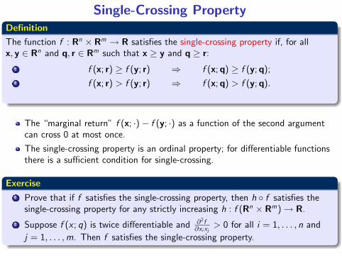
Single-Crossing PropertyDefinitionThe function f : Rn × Rm → R satisfies the single-crossing property if, for allx, y ∈ Rn and q, r ∈ Rm such that x ≥ y and q ≥ r:

1 f (x; r) ≥ f (y; r) ⇒ f (x;q) ≥ f (y;q);

2 f (x; r) > f (y; r) ⇒ f (x;q) > f (y;q).

The “marginal return” f (x; ·)− f (y; ·) as a function of the second argumentcan cross 0 at most once.

The single-crossing property is an ordinal property; for differentiable functionsthere is a suffi cient condition for single-crossing.

Exercise1 Prove that if f satisfies the single-crossing property, then h ◦ f satisfies thesingle-crossing property for any strictly increasing h : f (Rn × Rm)→ R.

2 Suppose f (x ; q) is twice differentiable and ∂2 f∂xi xj

> 0 for all i = 1, . . . , n andj = 1, . . . ,m. Then f satisfies the single-crossing property.

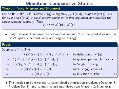
Monotone Comparative StaticsTheorem (easy Milgrom and Shannon)

Let f : Rn × Rm → R. Define x∗(q) = argmaxx∈R n f (x ; q). Suppose |x∗(q)| = 1for all q and f (x ; q) is quasi-supermodular in its first argument and satisfies thesingle-crossing property. Then

q ≥ r ⇒ x∗(q) ≥ x∗(r).

‘Easy’because it assumes the optimum is unique (thus, the proof does not use‘strict’quasi-supermodularity and single-crossing).

Proof.Suppose q ≥ r . Then:

f (x∗(r); r) ≥ f (x∗(q) ∧ x∗(r); r) by definition of x∗(q)

⇒ f (x∗(q) ∨ x∗(r); r) ≥ f (x∗(q); r) by quasi-supermodularity in x

⇒ f (x∗(q) ∨ x∗(r); q) ≥ f (x∗(q); q) by Single Crossing

⇒ x∗(q) ∨ x∗(r) = x∗(q) since |x∗(q)| equals 1⇒ x∗(q) ≥ x∗(r) by Question 2, PS4

This result can be extended to constrained optimization problems (Question 3,Problem Set 4), and to multi-valued optimizers (see Milgrom & Shannon).

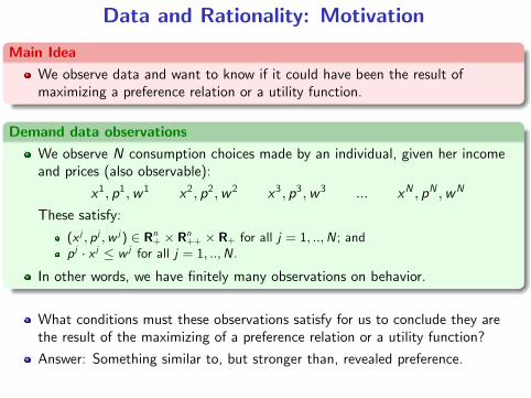
Data and Rationality: Motivation

Main IdeaWe observe data and want to know if it could have been the result ofmaximizing a preference relation or a utility function.

Demand data observationsWe observe N consumption choices made by an individual, given her incomeand prices (also observable):

x1, p1,w 1 x2, p2,w 2 x3, p3,w 3 ... xN , pN ,wN

These satisfy:

(x j , p j ,w j ) ∈ Rn+ × Rn++ × R+ for all j = 1, ..,N ; andp j · x j ≤ w j for all j = 1, ..,N .

In other words, we have finitely many observations on behavior.

What conditions must these observations satisfy for us to conclude they arethe result of the maximizing of a preference relation or a utility function?

Answer: Something similar to, but stronger than, revealed preference.

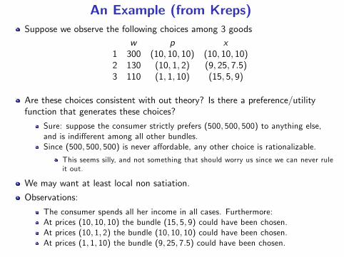
An Example (from Kreps)Suppose we observe the following choices among 3 goods

w p x1 300 (10, 10, 10) (10, 10, 10)2 130 (10, 1, 2) (9, 25, 7.5)3 110 (1, 1, 10) (15, 5, 9)

Are these choices consistent with out theory? Is there a preference/utilityfunction that generates these choices?

Sure: suppose the consumer strictly prefers (500, 500, 500) to anything else,and is indifferent among all other bundles.Since (500, 500, 500) is never affordable, any other choice is rationalizable.

This seems silly, and not something that should worry us since we can never ruleit out.

We may want at least local non satiation.

Observations:

The consumer spends all her income in all cases. Furthermore:At prices (10, 10, 10) the bundle (15, 5, 9) could have been chosen.At prices (10, 1, 2) the bundle (10, 10, 10) could have been chosen.At prices (1, 1, 10) the bundle (9, 25, 7.5) could have been chosen.

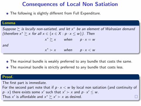
Consequences of Local Non SatiationThe following is slightly different from Full Expenditure.

LemmaSuppose % is locally non-satiated, and let x∗ be an element of Walrasian demand(therefore x∗ % x for all x ∈ {x ∈ X : p · x ≤ w}). Then

x∗ % x when p · x = w

andx∗ � x when p · x < w

The maximal bundle is weakly preferred to any bundle that costs the same.

The maximal bundle is strictly preferred to any bundle that costs less.

Proof.The first part is immediate.For the second part note that if p · x < w by local non satiation (and continuity ofp · x) there exists some x ′ such that x ′ � x and p · x ′ ≤ w .Thus x ′ is affordable and x∗ % x ′ � x as desired.

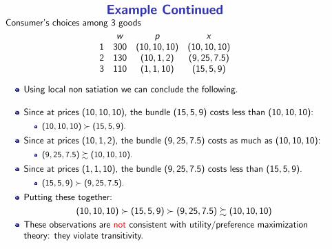
Example ContinuedConsumer’s choices among 3 goods

w p x1 300 (10, 10, 10) (10, 10, 10)2 130 (10, 1, 2) (9, 25, 7.5)3 110 (1, 1, 10) (15, 5, 9)

Using local non satiation we can conclude the following.

Since at prices (10, 10, 10), the bundle (15, 5, 9) costs less than (10, 10, 10):

(10, 10, 10) � (15, 5, 9).

Since at prices (10, 1, 2), the bundle (9, 25, 7.5) costs as much as (10, 10, 10):

(9, 25, 7.5) % (10, 10, 10).

Since at prices (1, 1, 10), the bundle (9, 25, 7.5) costs less than (15, 5, 9).

(15, 5, 9) � (9, 25, 7.5).

Putting these together:

(10, 10, 10) � (15, 5, 9) � (9, 25, 7.5) % (10, 10, 10)

These observations are not consistent with utility/preference maximizationtheory: they violate transitivity.

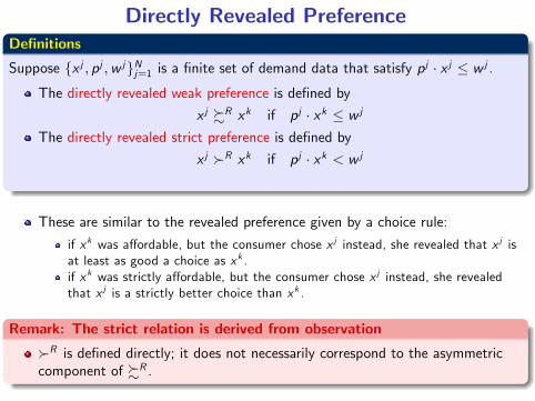
Directly Revealed PreferenceDefinitions

Suppose {x j , pj ,w j}Nj=1 is a finite set of demand data that satisfy pj · x j ≤ w j .The directly revealed weak preference is defined by

x j %R xk if pj · xk ≤ w j

The directly revealed strict preference is defined by

x j �R xk if pj · xk < w j

These are similar to the revealed preference given by a choice rule:

if x k was affordable, but the consumer chose x j instead, she revealed that x j isat least as good a choice as x k .if x k was strictly affordable, but the consumer chose x j instead, she revealedthat x j is a strictly better choice than x k .

Remark: The strict relation is derived from observation

�R is defined directly; it does not necessarily correspond to the asymmetriccomponent of %R .

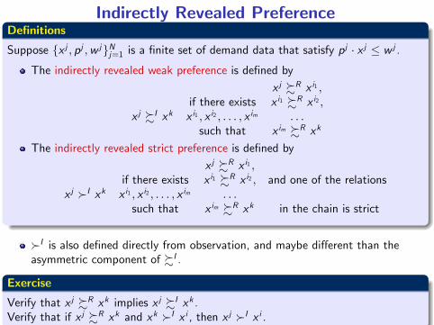
Indirectly Revealed PreferenceDefinitions

Suppose {x j , pj ,w j}Nj=1 is a finite set of demand data that satisfy pj · x j ≤ w j .The indirectly revealed weak preference is defined by

x j %R x i1 ,if there exists x i1 %R x i2 ,

x j %I xk x i1 , x i2 , . . . , x im . . .such that x im %R xk

The indirectly revealed strict preference is defined by

x j %R x i1 ,if there exists x i1 %R x i2 , and one of the relations

x j �I xk x i1 , x i2 , . . . , x im . . .such that x im %R xk in the chain is strict

�I is also defined directly from observation, and maybe different than theasymmetric component of %I .

Exercise

Verify that x j %R xk implies x j %I xk .Verify that if x j %R xk and xk �I x i , then x j �I x i .