A&A 616, A139 (2018)https://doi.org/10.1051/0004-6361/201833004c© ESO 2018

Astronomy&Astrophysics

SMA observations of polarized dust emission in solar-type Class 0protostars: Magnetic field properties at envelope scales

Maud Galametz1, Anaëlle Maury1,5, Josep M. Girart2,3, Ramprasad Rao4, Qizhou Zhang5, Mathilde Gaudel1,Valeska Valdivia1, Eric Keto5, and Shih-Ping Lai6

1 Astrophysics department, CEA/DRF/IRFU/DAp, Université Paris Saclay, UMR AIM, 91191 Gif-sur-Yvette, Francee-mail: galametz@cea.fr

2 Institut de Ciències de l’Espai (ICE, CSIC), Can Magrans, S/N, 08193 Cerdanyola del Vallès, Catalonia, Spain3 Institut d’Estudis Espacials de de Catalunya (IEEC), 08034 Barcelona, Catalonia, Spain4 Institute of Astronomy and Astrophysics, Academia Sinica, 645 N. Aohoku Pl, Hilo, HI 96720, USA5 Harvard-Smithsonian Center for Astrophysics, 60 Garden street, Cambridge MA 02138, USA6 Institute of Astronomy and Department of Physics, National Tsing Hua University, Hsinchu 30013, Taiwan

Received 12 March 2018 / Accepted 15 April 2018

ABSTRACT

Aims. Although from a theoretical point of view magnetic fields are believed to play a significant role during the early stages of starformation, especially during the main accretion phase, the magnetic field strength and topology is poorly constrained in the youngestaccreting Class 0 protostars that lead to the formation of solar-type stars.Methods. We carried out observations of the polarized dust continuum emission with the SMA interferometer at 0.87 mm to probethe structure of the magnetic field in a sample of 12 low-mass Class 0 envelopes in nearby clouds, including both single protostarsand multiple systems. Our SMA observations probed the envelope emission at scales ∼600−5000 au with a spatial resolution rangingfrom 600 to 1500 au depending on the source distance.Results. We report the detection of linearly polarized dust continuum emission in all of our targets with average polarization fractionsranging from 2% to 10% in these protostellar envelopes. The polarization fraction decreases with the continuum flux density, whichtranslates into a decrease with the H2 column density within an individual envelope. Our analysis show that the envelope-scalemagnetic field is preferentially observed either aligned or perpendicular to the outflow direction. Interestingly, our results suggest forthe first time a relation between the orientation of the magnetic field and the rotational energy of envelopes, with a larger occurrenceof misalignment in sources in which strong rotational motions are detected at hundreds to thousands of au scales. We also show thatthe best agreement between the magnetic field and outflow orientation is found in sources showing no small-scale multiplicity and nolarge disks at ∼100 au scales.

Key words. stars: formation – circumstellar matter – ISM: magnetic fields – polarization – techniques: polarimetric

1. Introduction

Understanding the physical processes at work during the earliestphase of star formation is key to characterize the typical out-come of the star formation process, put constraints on the effi-ciency of accretion and ejection mechanisms, and determine thepristine properties of planet-forming material. Class 0 objectsare the youngest accreting protostars Andre et al. 1993, 2000.The bulk of their mass resides in a dense envelope that is be-ing actively accreted onto the central protostellar embryo dur-ing a short main accretion phase (t < 105 yr; Maury et al. 2011;Evans et al. 2009). The physics at work to reconcile the order-of-magnitude difference between the large angular momentum ofprestellar cores (Goodman et al. 1993; Caselli et al. 2002) andthe rotation properties of the young main sequence stars (alsocalled the “angular momentum problem”; Bodenheimer 1995;Belloche 2013) is still not fully understood. It was proposed thatthe angular momentum could be strongly reduced by the frag-mentation of the core in multiple systems or the formation ofa protostellar disk and/or launch of a jet carrying away angularmomentum. None of these solutions, however, seem to be ableto reduce the angular momentum of the core’s material by therequired 5 to 10 orders of magnitude.

Magnetized models have shown that the outcome of thecollapse phase can be significantly modified through magneticbraking (Galli et al. 2006; Li et al. 2014). The role of magneticfields in Class 0 properties has also been investigated obser-vationally. A few studies have compared the observations ofClass 0 protostars to the outcome of models, either vanalytically(see, e.g., Frau et al. 2011) or from magneto-hydrodynamicalsimulations (see, e.g., Maury et al. 2010, 2018). These stud-ies have shown that magnetized models of protostellar forma-tion better reproduce the observed small-scale properties of theyoungest accreting protostars, for instance the lack of fragmen-tation and paucity of large (100< rdisk < 500 au) rotationallysupported disks (Maury et al. 2010, 2014; Enoch et al. 2011;Segura-Cox et al. 2016) observed in Class 0 objects.

The polarization of the thermal dust continuum emissionprovides an indirect probe of the magnetic field topology sincethe long axis of nonspherical or irregular dust grains is sug-gested to align perpendicular to the magnetic field direction(Lazarian 2007). Recently, the Planck Space Observatory pro-duced an all-sky map of the polarized dust emission at submil-limeter wavelengths, revealing that the Galactic magnetic fieldshows regular patterns (Planck Collaboration Int. XXXV 2016).

Open Access article, published by EDP Sciences, under the terms of the Creative Commons Attribution License (http://creativecommons.org/licenses/by/4.0),which permits unrestricted use, distribution, and reproduction in any medium, provided the original work is properly cited.

A139, page 1 of 22

A&A 616, A139 (2018)

Observations at better angular resolution obtained from ground-based facilities seem to indicate that the polarization patterns arewell ordered at the scale of Hii regions or molecular cloud com-plexes (Curran & Chrysostomou 2007; Matthews et al. 2009;Poidevin et al. 2010). Crutcher (2012) and references thereinprovides a review of magnetic fields in molecular clouds.

Few polarization observations have been performed tocharacterize the magnetic field topology at the protostellarenvelope scales where the angular momentum problem is rel-evant. Submillimeter interferometric observations of the polar-ized dust continuum emission with the Submillimeter Array(SMA; Ho et al. 2004) and Combined Array for Research inMillimeter-wave Astronomy (CARMA; Bock et al. 2006) inter-ferometers have led to the detections of polarized dust con-tinuum emission toward a dozen low-mass Class 0 protostars(Rao et al. 2009; Girart et al. 2006; Hull et al. 2014); in par-ticular these observations have led to the detection of lumi-nous and/or massive objects because of the strong sensitiv-ity limitations to detect a few percent of the dust continuumemission emitted by low-mass objects. By comparing the large-scale (∼20′′) and small-scale (∼2.5′′) B fields of protostars at1 mm (TADPOL survey), Hull et al. (2014) found that sourcesin which the large and small magnetic field orientations areconsistent tend to have higher fractional polarization, whichcould be a sign of the regulating role of magnetic fields dur-ing the infall of the protostellar core. No systematic relation,however, seems to exist between the core magnetic field di-rection and the outflow orientation (Curran & Chrysostomou2007; Hull et al. 2013; Zhang et al. 2014). An hourglass shapeof the magnetic line segments was observed in several proto-stellar cores (Girart et al. 1999, 2006; Lai et al. 2002; Rao et al.2009; Stephens et al. 2013). This hourglass pattern, which isprobably linked with the envelope contraction pulling the mag-netic field lines toward the central potential well, could de-pend strongly on the alignment between the core rotation axisand the magnetic field direction (Kataoka et al. 2012). Observa-tions with the Atacama Large Millimeter/submillimeter Array(ALMA) are now pushing the resolution and sensitivity enoughto probe down to 100 au scales in close-by low-mass Class 0 pro-tostars. In the massive (Menv∼20 M) binary protostar SerpensSMM1, these observations have revealed a chaotic magneticfield morphology affected by the outflow (Hull et al. 2017).In the solar-type Class 0 B335, they have, on the contrary, un-veiled very ordered topologies and there is a clear transition froma large-scale B-field parallel to the outflow direction to a stronglypinched B in the equatorial plane (Maury et al. 2018).

Whether or not magnetic fields play a dominant role in reg-ulating the collapse of protostellar envelopes needs to be furtherinvestigated from an observational perspective. In this paper, weanalyze observations of the 0.87 mm polarized dust continuumfor a sample of 12 Class 0 (single and multiple systems) proto-stars with the SMA interferometer (Ho et al. 2004) to increasethe current statistics on the polarized dust continuum emissiondetected in protostellar envelopes on 750–2000 au scales. Weprovide details on the sample and data reduction steps in Sect. 2.We study the continuum fluxes and visibility profiles and de-scribe the polarization results in Sect. 3. We analyze the polariza-tion fraction dependencies with density and the potential causesof depolarization in Sect. 4.1. In Sect. 4.2, we analyze the large-to small-scale B orientation and its variation with wavelength.We finally discuss the relation between the magnetic field ori-entation and both the rotation and fragmentation properties inthe target protostellar envelopes. A summary of this work is pre-sented in Sect. 5.

Fig. 1. Envelope mass vs. bolometric luminosity diagram fromAndre et al. (2000) and Maury et al. (2011). The small blacksquares and triangles are Class 0 and I protostars detected in theAquila rift, Ophiuchus, Perseus, and Orion regions (Bontemps et al.1996; Motte & André 2001; Andre et al. 2000; Maury et al. 2011;Sadavoy et al. 2014). The lines indicate the conceptual border zone be-tween the Class 0 and Class I stage, with Menv ∝ Lbol for the dashedline and Menv ∝ L0.6

bol for the dotted line. Blue lines with arrows repre-sent protostellar evolutionary tracks, computed for final stellar massesof 0.1, 0.3, 1, and 3M; the evolution proceeds from top left (objectswith large envelope masses slowly accreting) to bottom (the envelopemass and the accretion luminosity are rapidly decreasing). Our sam-ple is overlaid with the positions of protostars in our sample: B335 inyellow, IRAS16293 in purple, Perseus sources in green, and Cepheussources in light blue. The sample only contains low-mass Class 0 pro-tostars, except for SVS13-A. The Menv and Lbol are from Massi et al.(2008) for CB230, Launhardt et al. (2013) for B335, Crimier et al.(2010) for IRAS16293, Sadavoy et al. (2014), Ladjelate et al. (in prep.),and Maury et al. (in prep.) for the rest of the sources.

2. Observations and data reduction

2.1. Sample description

Our sample contains 12 protostars that include single objects aswell as common-envelope multiple systems and separate enve-lope multiple systems (following the classification proposed byLooney et al. 2000). Figure 1 shows the location of the protostarsin an envelope mass (Menv) versus bolometric luminosity (Lbol)diagram (Bontemps et al. 1996; Maury et al. 2011). With mostof the object mass contained in the envelope, our selection is arobust sample of low-mass Class 0 protostars. Only SVS13-Acan be classified as a Class I protostar. Details on each object areprovided in Table 1 and in the Appendix.

2.2. SMA 0.87 mm observations

Observations of the polarized dust emission of nine low-massprotostars at 0.87 mm were obtained using the SMA (Projects2013A-S034 and 2013B-S027, PI: A. Maury) in the compactand subcompact configuration. To increase our statistics, wealso included SMA observations from three additional sourcesfrom Perseus (NGC 1333 IRAS4A and IRAS4B) and Ophiuchus(IRAS16293) observed in 2004 and 2006 (Projects 2004-142 and2006-09-A026, PI: R. Rao; Project 2005-09-S061, PI: D.P. Mar-rone). The observations of NGC 1333 IRAS4A and IRAS16293

A139, page 2 of 22

M. Galametz et al: Polarized dust emission in solar-type Class 0 protostars

Table 1. Properties of the sample.

Name Cloud Distancea Class Multiplicityb Observation Phase Reference Center

B335 isolated 100 pc Class 0 Single 19h37m00.9s +0734′09′′.6SVS13 Perseus 235 pc Class 0/I Multiple (wide) 03h29m03.1s +3115′52′′.0HH797 Perseus 235 pc Class 0 Multiple 03h43m57.1s +3203′05′′.6L1448C Perseus 235 pc Class 0 Multiple (wide) 03h25m38.9s +3045′14′′.9L1448N Perseus 235 pc Class 0 Multiple (close and wide) 03h25m36.3s +3044′05′′.4L1448-2A Perseus 235 pc Class 0 Multiple (close and wide) 03h25m22.4s +3045′12′′.2IRAS03282 Perseus 235 pc Class 0 Multiple (close) 03h31m20.4s +3045′24′′.7NGC 1333 IRAS4A Perseus 235 pc Class 0 Multiple (close) 03h29m10.5s +3113′31′′.0NGC 1333 IRAS4B Perseus 235 pc Class 0 Single 03h29m12.0s +3113′08′′.0IRAS16293 Ophiuchus 120 pc Class 0 Multiple (wide) 16h32m22.9s −2428′36′′.0L1157 Cepheus 250 pc Class 0 Single 20h39m06.3s +6802′15′′.8CB230 Cepheus 325 pc Class 0 Binary (close) 21h17m40.0s +6817′32′′.0

Notes. (a)Distance references are Knude & Hog (1998), Stutz et al. (2008), Hirota et al. (2008), Hirota et al. (2011), Looney et al. (2007) andStraizys et al. (1992). (b)Multiplicity derived from Launhardt (2004) for IRAS03282 and CB230, Rao et al. (2009) for IRAS16293, Palau et al.(2014) for HH797, Evans et al. (2015) for B335 and from the CALYPSO survey dust continuum maps at 220 GHz (PdBI; see http://irfu.cea.fr/Projets/Calypso/, and Maury et al. 2014) for the rest of the sources.

are presented in Girart et al. (2006) and Rao et al. (2009),respectively. Marrone (2006) and Marrone & Rao (2008) providea detailed description of the SMA polarimeter system, but weprovide a few details on the SMA and the polarization de-sign below. The SMA has eight antennas. Each optical path isequipped with a quarter-wave plate (QWP), an optical elementthat adds a 90 phase delay between orthogonal linear polar-izations and is used to convert the linear into circular polariza-tion. The antennas are switched between polarizations (QWP arerotated at various angles) in a coordinated temporal sequenceto sample the various combinations of circular polarizations oneach baseline. The 230, 345, and 400 band receivers are in-stalled in all eight SMA antennas. Polarization can be mea-sured in single-receiver polarization mode and in dual-receivermode when two receivers with orthogonal linear polarizationsare tuned simultaneously. In this dual-receiver mode, all correla-tions (the parallel-polarized RR and LL and the cross-polarizedRL and LR; with R and L for right circular and left circular,respectively) are measured at the same time. Both polarizationmodes were used in our observations. This campaign was usedto partly commission the dual-receiver full polarization modefor the SMA. A fraction of the data was lost during this pe-riod owing to issues with the correlator software. Frequent ob-servations of various calibrators were interspersed to ensure thatsuch issues were detected as early as possible to minimize dataloss.

2.3. Data calibration and self-calibration

We performed the data calibration in the IDL-based soft-ware Millimeter Interferometer Reduction (MIR) and the datareduction package MIRIAD1. The calibration includes an initialflagging of high system temperatures Tsys and other wrong visi-bilities, a bandpass calibration, a correction of the cross-receiverdelays, a gain, and a flux calibration. The various calibrators ob-served for each of these steps and the list of antennae used forthe observations are summarized in Table 2. The polarization

1 https://www.cfa.harvard.edu/sma/miriad/

calibration was performed in MIRIAD. Quasars were observed tocalculate the leakage terms: the leakage amplitudes (accuracy:∼0.5%) are <2% in the two sidebands for all antenna except forseven than can reach a few percent. Before the final imaging, weused an iterative procedure to self-calibrate the Stokes I visibilitydata.

2.4. Deriving the continuum and polarization maps

The Stokes parameters describing the polarization state are de-fined as

S =

IQUV

, (1)

with Q and U the linear polarization and V the circular polariza-tion. We used a robust weighting of 0.5 to transform the visibilitydata into a dirty map. The visibilities range from 5 kλ to 30 kλin seven sources (B335, SVS13, HH797, L1448C, IRAS03282,L1157, and CB230) and 10 kλ to 80 kλ for the other five sources.Visibilities beyond 80 kλ are available for NGC 1333 IRAS4Abut not used to allow an analysis of comparable scales for all oursources. The Stokes I dust continuum emission maps are shownin Fig. 2. The Stokes Q and U maps are shown in Fig. B.1. Theircombination probes the polarized component of the dust emis-sion. The synthesized beams and rms of the cleaned maps areprovided in Table 3. We note that because of unavoidable miss-ing flux and the dynamic-range limitation, the rms of the Stokes Imaps are systematically higher than those of Stokes Q and U.Following the self-calibration procedure, the rms of the contin-uum maps have decreased by 10–45%.

The polarization intensity (debiased), fraction and angle arederived from the Stokes Q and U as follows:

Pi =

√Q2 + U2 − σ2

Q,U , (2)

pfrac = Pi / I, (3)

PA = 0.5 × arctan(U/Q), (4)

A139, page 3 of 22

A&A 616, A139 (2018)

Table 2. Details on the observations.

Date Modea Flux Bandpass Gain Polarization Antennacalib. calib. calib. calib. used

Dec 05 2004 Single Rx–Single BW Ganymede 3c279 3c84 3c279 1, 2, 3, 5, 6, 8Dec 06 2004 Single Rx–Single BW Ganymede 3c279 3c84 3c279 1, 2, 3, 5, 6, 8April 08 2006 Single Rx–Single BW Callisto 3c273 1517−243, 1622−297 3c273 1, 2, 3, 5, 6, 7, 8Dec 23 2006 Single Rx–Single BW Titan 3c279 3c84 3c279 1, 2, 3, 4, 5, 6, 7Aug 26 2013 Single Rx–Double BW Neptune 3c84 1927+739, 0102+584 3c84 2, 4, 5, 6, 7, 8Aug 31 2013 Dual Rx–Autocorrel Callisto 3c84 1751+096, 1927+739, 0102+584, 3c84 3c84 2, 4, 5, 6, 7, 8Sept 1 2013 Dual Rx–Autocorrel Callisto 3c84 1927+739, 0102+584 3c84 2, 4, 5, 6, 7, 8Sept 2 2013 Dual Rx–Autocorrel Callisto 3c454.3 1927+739, 0102+584,3c84 3c84 2, 4, 5, 6, 7, 8Sept 7 2013 Dual Rx–Full pol. Callisto 3c454.3 3c84, 3c454.3 3c454.3 2, 4, 5, 6, 7, 8Dec 7 2013 Dual Rx–Full pol. Callisto 3c84 3c84 3c84 2, 4, 5, 6, 7, 8Feb 24 2014 Dual Rx–Full pol. Callisto 3c279 3c84, 3c279, 0927+390 3c279 1, 2, 4, 5, 6, 7Feb 25 2014 Dual Rx–Full pol. Callisto 3c84 3c84 3c84 1, 2, 4, 5, 6, 7

Notes. (a) Rx = Receiver; BW = bandwidth.

withσQ,U the average rms of the Q and U maps. We applied a 5σcutoff on Stokes I and 3σ cutoff on Stokes Q and U to only se-lect locations where polarized emission is robustly detected. Thepolarization intensity and fraction maps are provided in Fig. B.1.

3. Results

3.1. 0.87 mm continuum fluxes

The 0.87 mm dust continuum maps are presented in Fig. 2 (theStokes I dust continuum emission is described in Appendix A).We overlay the outflow direction (references from the literaturecan be found in Table 6). We provide the peak intensities andintegrated 0.87 mm flux densities in Table 4. We also provide theassociated masses calculated using the following relation fromHildebrand (1983):

M =S ν D d2

κν Bν(T ), (5)

where Sν is the flux density, D the dust-to-gas mass ratio as-sumed to be 0.01, d the distance to the protostar, κν the dust opac-ity (tabulated in Ossenkopf & Henning (1994), 1.85 cm2 g−1

at 0.87mm), and Bν(T) the Planck function. We choose a dusttemperature of 25K, coherent with that observed at 1000 au inIRAS16293 by Crimier et al. (2010). A dust temperature of 50Kwould only decrease the gas mass reported in Table 4 by a factorof ∼2.

The sensitivity of SMA observations decreases outside theprimary beam (i.e., 34′′) and the coverage of the shortestbaselines is not complete. We thus expect that only partof the total envelope flux is recovered by our SMA obser-vations, especially for the closest sources. To estimate howmuch of the extended flux is missing, we compare the SMAfluxes with those obtained with the SCUBA single-dish in-strument. Di Francesco et al. (2008) provided a catalog of 0.87mm continuum fluxes and peak intensities for a large rangeof objects observed with SCUBA at 450 and 850 µm, includ-ing our sources. The SCUBA integrated flux uncertainties aredominated by the 15% calibration uncertainties while the abso-lute flux uncertainty for the SMA is <10%. Results are summa-rized in Table 5. We find that the SMA total flux, integrated in thereconstructed cleaned maps of the sources, accounts for 9–18%

of the SCUBA total fluxes. This is consistent with the results ofthe PROSAC low-mass protostar survey for which only 10–20%of the SCUBA flux is recovered with the SMA (Jørgensen et al.2007). As far as the dust continuum peak flux densities are con-cerned, if we rescale the SCUBA peak flux densities to thatexpected in the SMA beam, assuming that the intensity scaleswith radius (i.e., a density dependence ρ ∝ r−2), we find thatSCUBA and SMA peak flux densities are consistent with eachother. This means that most of the envelope flux is recovered atSMA beam scales. The largest discrepancies appear for B335,NGC 1333 IRAS4A, and NGC 1333 IRAS4B. For B335, theSCUBA value is twice that derived with SMA. This indicatesthat for this source, one of the closest of our sample, part of theSMA continuum flux might be missing even at the peak of con-tinuum emission, and the polarization fraction could be lowerthan that determined from the SMA observations (Sect. 3). ForNGC 1333 IRAS4A and IRAS4B, the inverse is observed: theSMA peak value is two and four times larger than the rescaledSCUBA. The two sources are the most compact envelopes of thesample (Looney et al. 2003; Santangelo et al. 2015). The differ-ence is thus probably due to the compact protostellar cores beingdiluted in the large SCUBA beam and possible contaminationof the SCUBA fluxes because NGC 1333 IRAS4A and B areboth located within a long (1′× 40′′) filamentary cloud extend-ing southeast-northwest (Lefloch et al. 1998).

3.2. Analysis of the Stokes I visibilities

Part of the extended dust continuum emission is lost during thereconstruction of the final image itself, since an interferometercan only sparsely sample Fourier components of different spa-tial frequencies of the incoming signal. To analyze the impact ofthe map reconstruction on the flux values derived, we can com-pare the flux densities derived from the reconstructed map withthose deduced directly from the visibility amplitude curves. TheStokes I amplitudes of the visibilities, averaged every 120s, arepresented in Fig. 3. The sample includes three wide binary ob-jects resolved by our SMA observations, i.e., L1448N, SVS13,and IRAS16293. We use the visibility data to separate the bi-nary sources. As the sources cannot be modeled using a simpleGaussian fitting, we use the MIRIAD/imsub function to producea subimage containing L1448N-A, SVS13-A, and IRAS16293-B from the cleaned image. We then use MIRIAD/uvmodel to

A139, page 4 of 22

M. Galametz et al: Polarized dust emission in solar-type Class 0 protostars

Fig. 2. SMA 850 µm Stokes I continuum maps. Color scales are in mJy/beam. Contours at [−3, 5, 10, 20, 30, 40, 50, 60, 70, 80, 90, 100] σ appearin blue. The filled ellipses in the bottom left corner indicate the synthesized beam of the SMA maps. Their sizes are reported in Table 3. The bluearrows indicate the outflow direction. The B orientations (derived from the polarization angles assuming a 90 rotation) are overlaid on the Stokes Imap. Red bars show >3σ detections. We also indicate the >2σ detections with orange bars but these detections are not used for this analysis

subtract these sources from the visibility data and make an imageof L1448N-B, SVS13-B, and IRAS16293-A from the modifiedvisibility datasets. We proceed the same way to map L1448N-A,SVS13-A, and IRAS16293-B, independently. The separated vis-ibility profiles are shown in Fig. 3. The region mapped aroundNGC 1333 IRAS4B contained IRAS4A (outside the primarybeam) and IRAS4B2 located about 10′′ east of IRAS4B. Thesetwo sources are also isolated and removed from the visibilitydata presented in Fig. 3.

We use a Gaussian fittingv method to fit the visibilities andextrapolate these models at 0 kλ to derive the integrated 0.87 mmcontinuum fluxes. The fluxes derivedv from the visibility am-plitude curves are reported in Table 4. The fluxes derived fromthe visibility amplitude curves are close but, as expected, sys-tematically larger (on average 2.2 times) than those derived onthe reconstructed maps. We also indicate the 0.87 mm contin-uum fluxes of L1448N-B and SVS13-B (the sources located atthe phase center) in Table 4. We find that SVS13-A and B have

A139, page 5 of 22

A&A 616, A139 (2018)

Table 3. Characteristics of the SMA maps.

Name Synthesized beam rms (mJy/beam)Ia Q U

B335 4′′.8×4′′.1 (84) 4.6 4.0 4.3SVS13 4′′.9×4′′.3 (-88) 7.0 3.0 3.1HH797 4′′.7×4′′.3 (89) 4.2 1.9 1.8L1448C 4′′.7×4′′.4 (87) 4.7 3.6 3.7L1448N 2′′.6×2′′.4 (55) 5.5 3.3 3.0L1448-2A 2′′.5×2′′.2 (49) 1.8 1.6 1.6IRAS03282 4′′.8×4′′.3 (88) 5.3 3.3 3.5NGC 1333 IRAS4A 2′′.0×1′′.4 (-46) 18.7 7.5 8.0NGC 1333 IRAS4B 2′′.2×1′′.7 (10) 9.0 2.2 2.3IRAS16293 3′′.0×1′′.8 (-6) 10.4 5.6 6.0L1157 5′′.9×4′′.6 (1) 8.8 6.4 7.6CB230 6′′.1×4′′.2 (7) 5.5 4.11 4.0

Notes. (a) Stokes I rms noise values come from the maps obtained afterself-calibration.

similar fluxes while L1448N-B is four times brighter thanL1448N-A.

For five sources, observations sampled baselines above40 kλ, i.e., sampling smaller spatial scales and most compactcomponents of the envelope. We produce new maps of thesesources using only visibilities that have a radius in the uv planelarger than 40 kλ. We use a natural weighting scheme to producethe maps in order to achieve the highest point-source sensitiv-ity. These maps are shown in Fig. 4. The flux densities of thecompact components are ∼150, 25, 580, 530, and 1120 mJy forL1448N, L1448-2A, NGC 1333 IRAS4A, NGC 1333 IRAS4B,and IRAS16293, respectively; for L1448N and L1448-2A, thecompact component only accounts for less than one-tenth ofthe total flux; and for NGC 1333 IRAS4A and IRAS16293for one-quarter of the total flux. This means that for these ob-jects most of the mass is still in the large-scale envelope ratherthan in a massive disk, and that our SMA observations al-low us to trace the polarized emission at the envelope scaleswhere most of the mass resides with only a little contaminationfrom a possible central protostellar disk. The visibility profileof NGC 1333 IRAS4B is the flattest in our sample (Fig. 3).One-third of the total 0.87 mm flux is contained in the com-pact component. This flat visibility profile is consistent withthose analyzed in Looney et al. (2003) and those obtained atboth 1 mm and 3 mm by the IRAM-PdBI CALYPSO2 sur-vey. The profile drops steeply at uv distances larger than 60 kλ,which suggests that NGC 1333 IRAS4B either has a compact(FWHM <6′′) envelope or that its submillimeter emission atscales 3–6′′ is dominated by the emission from a large Gaus-sian disk-like structure. We note that both NGC 1333 IRAS4Aand IRAS4B have very compact envelopes (envelope outer radii< 6′′) as seen with the PdBI observations at 1 mm and 3 mm(Maury et al., in prep).

3.3. Polarization results

Figure B.1 shows the maps of the Stokes Q and U parametersand the polarization intensity and polarization fraction maps ob-tained when combining these maps. The peak polarization in-tensities and the median polarization fractions (defined as theunweighted ratio of the median polarization intensity to the flux

2 http://irfu.cea.fr/Projets/Calypso

intensity) are listed in Table 4. In spite of their low luminos-ity at SMA scales, we detect linearly polarized continuum emis-sion in all the low-mass protostars, even using a conservative3σ threshold. Median polarization fractions range from a few% for IRAS16293 and L1448N to 10% for B335. We only ob-tain a weak 2σ detection toward the northeastern companionof SMME/HH797 (around 03:43:57.8; +32:03:11.3). This ob-ject was classified as a Class 0 proto-brown dwarf candidate byPalau et al. (2014). When polarization is detected in the center,we observe that the polarization fraction drops toward this cen-ter. For HH797, L1448C, L1448-2A, and IRAS03282, we de-tect polarization in the envelope at distances between 700 and1600 au from the Stokes I emission peak, but not in the centeritself. The absence of polarization could be linked with an av-eraging effect at high column density in the beam and/or alongthe line of sight in those objects. We analyze potential causes fordepolarization in Sect. 4.1.

4. Analysis and discussion

4.1. Distribution of the polarized emission

Polarization is detected in all of our maps, but not alwaystoward the peak of dust continuum emission (Stokes I). Aconstant polarization fraction would predict, on the contrary,that the polarized intensity scales as Stokes I. Yet, polariza-tion holes or depolarization are often observed in the high-density parts of star-forming molecular cores and protostellarsystems (Dotson 1996; Rao et al. 1998; Wolf et al. 2003;Girart et al. 2006; Tang et al. 2013; Hull et al. 2014). We ana-lyze the distribution of both polarized fraction and intensity inthis section in order to probe if and where depolarization isobserved.

4.1.1. Variation of the polarized fraction with environment

For sources in which polarization is detected within the central5′′, we observe a drop in the polarization fraction (Fig. B.1). Toquantify this decrease, we analyze how the polarization fractionvaries as a function of the 0.87 mm flux density. We first regener-ate our polarization maps with a homogeneous synthesized beamof 5.5′′ in all our sources, using independent pixels of one-thirdthe synthesized beam (1.8′′). IRAS 4A and B are not includedin this analysis because their dust continuum emission is barelyresolved at 5.5′′. L1448-2A is not included either since polar-ization is no longer robustly detected at this new resolution. Therelation linking pfrac versus the Stokes I flux density in each indi-vidual protostellar envelope is shown in Fig. 5 (top). The contin-uum flux densities are normalized to the peak intensity for eachobject to allow a direct comparison. We observe a clear depolar-ization toward inner envelopes with higher Stokes I fluxes andthere is a polarization fraction ∝ I−0.6 for B335 down to ∝ I−1.0

for L1448N or HH7973. Those coefficient are consistent withresults from the literature: the polarization fraction has, for in-stance, been found ∝ I−0.6 in Bok globules (Henning et al. 2001),∝ I−0.7−I−0.8 in dense cores (Matthews & Wilson 2000), anddown to ∝ I−0.97 in the main core of NGC 2024 FIR 5 (Lai et al.2002).

Since polarization holes are usually associated with a high-density medium, we also analyze how the polarization fractionvaries as a function of the gas column density N(H2). We assumethat the emission at 0.87 µm is optically thin. The column den-

3 A constant polarized flux gives a polarization fraction ∝ I−1.

A139, page 6 of 22

M. Galametz et al: Polarized dust emission in solar-type Class 0 protostars

Table 4. 0.87 mm integrated flux densities, source sizes, polarization intensities, and fractions.

Name On the 0.87 mm reconstructed maps From the visibility amplitude curveFlux densitya Mass Peak intensity Peak Pi

b pfracc 0.87 mm flux density

(Jy) (M) (Jy/beam) (mJy/beam) (%) (Jy)

B335 0.21±0.04 0.02 0.24 25.3 10.5 0.51±0.05SVS13 1.40±0.28 0.29 1.06 14.8 2.5 1.54±0.15d

HH797 0.47±0.09 0.10 0.71 5.7 3.0 0.94±0.09L1448C 0.57±0.11 0.11 0.65 12.5 – 1.00±0.01L1448N 1.50±0.30 0.31 1.34 20.3 2.7 1.93±0.19d

L1448-2A 0.34±0.07 0.07 0.27 5.7 – 0.48±0.05IRAS03282 0.44±0.09 0.09 0.65 9.9 – 1.17±0.12NGC 1333 IRAS4A 2.38±0.48 0.50 2.57 77.3 8.8 6.79±0.68NGC 1333 IRAS4B 1.42±0.28 0.30 2.89 14.9 4.7 4.10±0.41IRAS16293 4.81±0.96 0.26 3.83 39.2 1.7 5.96±0.60d

L1157 0.43±0.09 0.10 0.71 31.4 4.5 1.07±0.11CB230 0.22±0.04 0.09 0.37 14.3 6.4 0.58±0.06

Notes. (a)Flux density estimated within the central 6000 au for SVS13, 3000 au for other sources. (b)Not all the sources have an intensity peakco-spatial with the polarized intensity peak. (c)Polarization fraction defined as the unweighted ratio of the median polarization to total flux. (d)Thevisibility data allows us to separate the two components of wide binaries. The fluxes are those of the object located at the phase center, e.g.,L1448N-B, SVS13-B and IRAS16293-A.

Table 5. Comparison with SCUBA observations from Di Francesco et al. (2008).

Name SCUBA 850 µm Comparison SMA / SCUBAPeak intensity Effective radius Flux density Rescaled peak intensitya Peak intensity ratio Total flux ratio

(Jy/beam) (′′) (Jy) (Jy/SMA beam) SMA/SCUBA SMA/SCUBA

B335 1.45±0.14 34.5 2.38±0.36 0.46±0.07 0.52±0.09 0.09±0.02HH797 1.76±0.18 43.2 4.67±0.70 0.57±0.09 1.24±0.22 0.12±0.03L1448C 2.37±0.24 43.5 4.15±0.62 0.77±0.12 0.84±0.15 0.14±0.03L1448N 5.46±0.55 49.3 10.18±1.53 0.96±0.14 1.27±0.23 0.15±0.04L1448-2A 1.41±0.14 36.8 2.24±0.34 0.24±0.04 0.97±0.17 0.15±0.04IRAS03282 1.30±0.13 45.2 2.28±0.34 0.42±0.06 1.54±0.28 0.18±0.04NGC 1333 IRAS4A 11.4±0.11 38.5 14.4±2.16 1.40±0.21 1.83±0.33 0.17±0.04NGC 1333 IRAS4B 5.46±0.55 40.7 8.90±1.34 0.75±0.11 3.83±0.69b 0.16±0.04IRAS16293 20.2±0.20 56.8 29.5±4.43 3.43±0.51 1.12±0.20 0.16±0.04L1157 1.58±0.16 42.4 2.46±0.37 0.59±0.09 1.20±0.22 0.17±0.04CB230 1.22±0.12 43.2 2.35±0.35 0.45±0.07 0.82±0.15 0.09±0.02

Notes. (a)In order to estimate what the peak intensity of the SCUBA maps would correspond to in a SMA beam, we considered that the envelopefollows a r−2 density profile, thus that the intensity would scale in 1/r. The SMA beam for each source is provided in Table 3. The SCUBA FWHMat 850 µm is 14′′. SVS13 is not included in the table because SVS13-A and B are not resolved by SCUBA. (b)This high value can be explained bythe very flat intensity profile of the source that is barely resolved in our SMA observations (see Fig. 3).

sity is derived using the following formula from Schuller et al.(2009):

N(H2) =S ν

D µH2 mH Ω κν Bν(T ), (6)

where S ν is the flux density, µH2 the molecular weight of the ISM(µH2=2.8; from Kauffmann et al. 2008), mH the mass of an hy-drogen atom, Ω the solid angle covered by the beam, κν the dustopacity (tabulated in Ossenkopf & Henning 1994, 1.85 cm2 g−1 at0.87mm), and Bν(T ) the Planck function at a dust temperature T .The dust-to-gas mass ratioD is assumed to be 0.01.

The temperature is not constant throughout the object en-velopes. We assume that the temperature profile in optically thinouter envelopes follows T(r)∝ r−0.4 and we scale the profiles usingthe protostellar internal luminosities (Terebey et al. 1993),

T = 38 L0.2int

( r100 au

)−0.4. (7)

Internal luminosities Lint are calculated from Herschel GouldBelt Survey in Sadavoy et al. (2014) for the Perseus sources andfrom Maury et al. (in prep) for the other sources. The value Lintis approximated to the bolometric luminosity if no internal lumi-nosity could be found in the literature. Figure 5 (bottom) presentsthe dependency of pfrac with local column density. Even if the re-lation observed presents a large scatter, our results confirm thatthe polarization fraction decreases with increasing column den-sity in the envelopes of our sample.

Along with the polarization fraction variations, the distribu-tion of polarized emission intensities can also help us determinethe cause of depolarization. The SCUBAPOL observations haveshown that the polarization intensity can decrease at high den-sities (Crutcher et al. 2004). We do not observe such a trend inour sample. In Fig. 5, the slope of the polarization fraction re-lation with the dust continuum intensity is close to −1 or flatterfor most sources. This means that the polarization intensity is

A139, page 7 of 22

A&A 616, A139 (2018)

Fig. 3. Stokes I visibility amplitude as a function of uv distance (in units of kλ). The open squares are the amplitudes of the visibilities channel-averaged and time-averaged every 120s. The black squares are derived averaging these amplitudes of the visibilities in 6 kλ bins for L1448N,L1448-2A, NGC 1333 IRAS4A, IRAS4B, and IRAS16293 and 3 kλ bins for the other sources. For the wide-binary L1448N, SVS13, andIRAS16293, we model and isolate the two sources separately. For IRAS4B, we also isolate and remove NGC 1333 IRAS4B2 from the visi-bility data.

constant and even increases (i.e., B335, SVS13, or IRAS16293)toward the central regions (see also the polarization intensityand fraction maps provided in Fig. B.1). These results suggestthat for these sources, the decrease of the polarization fractionin the center is not linked to a full depolarization, but could in-dicate a variation in the polarization efficiency itself (see nextsection).

4.1.2. Potential causes for depolarization

Observations and models or simulations (Padoan et al. 2001;Bethell et al. 2007; Falceta-Gonçalves et al. 2008; Kataoka et al.2012) have shown that depolarization can be linked with bothgeometrical effects (e.g., averaging effects linked with the com-plex structure of the magnetic field along the line of sight) andphysical effects (e.g., collisional/mechanical disalignment, lowergrain alignment efficiency, and variation of the grain population).

We discuss here some of these depolarization effects. We note thatour sample is sensitivity limited, which means that there is a poten-tial bias toward strong polarization intensities. We also note thatthe polarized emission presented in this paper comes from the en-velope and that we are not sampling the polarized (or unpolarized)emission from the inner (<500 au) envelope.

Geometrical effects. Our SMA observations recover polarizedemission from previously reported polarization holes observedwith single-dish observations. Observations of B335 and CB230at a 2200 au resolution using SCUBAPOL (Holland et al. 1999)performed by Wolf et al. (2003) show that the polarization frac-tion decreases from 6–15% in the outer parts of the cores to a few%, thus at scales in which 3–10% polarization is detected withthe SMA (see Fig. 6 for an illustration in CB230). The centraldepolarization observed by Wolf et al. (2003) in B335 andCB230 is thus partially due to beam averaging effects or

A139, page 8 of 22

M. Galametz et al: Polarized dust emission in solar-type Class 0 protostars

L1448N L1448-2A

IRAS 4A IRAS 4B

IRAS 16293

A

B

A

B

4B

4B2

Fig. 4. 345GHz dust continuum emission in L1448N, L1448-2A,Fig. 4. 345GHz dust continuum emission in L1448N, L1448-2A,NGC 1333 IRAS4A, NGC 1333 IRAS4B, and IRAS16293 when onlyvisibilities above 40 kλ are kept. We apply a natural weighting to pro-duce these maps. Contours at [5,20,50]σ appear in blue. The beam sizesare ∼1′′.9×1′′.2.

mixing of the polarized signal along the line of sight, an envelopepattern that our SMA resolution now allows us to recover. Re-cent polarization observations of B335 with ALMA at evenhigher resolution by Maury et al. (2018) have confirmed thatpolarization is still detected toward the center of the B335 en-velope at 0.5–5′′ scales, which is a sign that the dust emis-sion stays polarized (p ∼ 3–7%) at small scales in high-densityregions.

Optical depth effects. As already reported in Girart et al. (2006),a two-lobe distribution of the polarization intensity is detectedtoward NGC 1333 IRAS4A. We report a similar two-lobe struc-ture for the first time in NGC 1333 IRAS4B and detect peaksof polarization intensity on each side of the north-south out-flow. Liu et al. (2016) have found that the polarization inten-sity of NGC 1333 IRAS4A observed at 6.9 mm has a moretypical distribution in which the polarization intensity peaks to-ward the source center; these authors have attributed this vari-ation of the polarization distribution with wavelength to opticaldepth effects. Our temperature brightnesses rather suggest thatthe 0.87 mm emission is optically thin at the envelope scalesprobed in this paper, for all our objects. We note that model-ing the magnetic field in NGC 1333 IRAS4A, Gonçalves et al.(2008) showed that strong central concentrations of magneticfield lines could reproduce a two-lobe structure in the polarizedintensity distribution.

Grain alignment, grain growth. Several studies of dense molecu-lar clouds or starless cores have shown that the slope of the polar-ization degree can reach values of −1 (as in some of our objects)or lower with respect to AV or I/Imax and interpret this slope

Fig. 5. Polarization fractions as a function of Stokes I continuum inten-sities at 0.87 mm (top panel) or as a function of the H2 column densities(bottom panel). Maps have been regenerated to share a common synthe-sized beam of about 5.5′′ and rebinned to have a grid with a commonpixel size of 1.8′′. The continuum flux densities plotted in the top panelare in units of Jy/beam but are normalized to the peak intensity for eachobject. The solid lines are the best fit to the function pfrac ∝ (I/Imax)a. TheH2 column densities plotted in the bottom panel are in units of cm−2 andare derived using Eqs. (5) and (6).

as a sign of a decrease or absence of grain alignment at higherdensities (Alves et al. 2014; Jones et al. 2015, 2016). Even ifthis is not the case in this work because our objects all havea central heating source, the degree of polarization we de-tect is still extremely sensitive to the efficiency of grain align-ment, which is itself very sensitive to the grain size distribution

A139, page 9 of 22

A&A 616, A139 (2018)

Fig. 6. Left: SCUBA 0.85 mm continuum maps with polarization orien-tation overlaid from Wolf et al. (2003). The contour lines indicate 20%,40%, 60%, and 80% of the maximum intensity. Right: zoom-in into thescales covered with the SMA at 0.87 mm. The contours are the samethan in Fig. 2. For both, the bar length is proportional to the polariza-tion fraction.

and potential grain growth (Bethell et al. 2007; Pelkonen et al.2009; Brauer et al. 2016). This grain growth has already beensuggested in Class 0 protostars such as L1448-2A or L1157(Kwon et al. 2009), in which there is a faster grain growth towardthe central regions. More observations combining various sub-millimeter wavelengths at various scales will help us probe thedust spectral index throughout the envelope, analyze the scalesat which grain growth is expected (Chacón-Tanarro et al. 2017),probe the various environmental dependencies of the grain align-ment efficiency (Whittet et al. 2008), and observationally con-strain the dependence on the polarization degree and the grainsize as predicted for instance by radiative torque models (seeBethell et al. 2007; Hoang & Lazarian 2009; Andersson et al.2015; Jones et al. 2015).

4.2. Orientation of the magnetic field

The B-field lines are inferred from the polarization angles by ap-plying a 90 rotation. The mean magnetic field orientations inthe central 1000 au are provided in Table 6. The B orientation isoverlaid with red bars in Fig. 2. We also show the >2σ detections(orange bars). Although these are subject to higher uncertaintieswe stress that they are mostly consistent with the neighboring3σ detection line segments. For robustness, however, these lowersignificance detections are not used in this analysis. Under flux-freezing conditions, the pull of field lines in strong gravitationalpotentials is expected to create an hourglass morphology of themagnetic field lines, centered around the dominant infall direc-tion, during protostellar collapse. Using CARMA observations,Stephens et al. (2013) showed that in L1157, the full hourglassmorphology becomes apparent around 550 au. Using SMA ob-servations, Girart et al. (2006) also observed this hourglass shapein NGC 1333 IRAS4A. The resolution we select for this analy-sis of B at envelope scale is not sufficient to reveal the hourglassmorphology in most of our objects. Only one of our sources,L1448-2A, shows hints of an hourglass shape at envelope scales(see Fig. 2) but the nondetection of polarization in the northernquadrant does not allow us to detect a full hourglass pattern inthis source. Better sensitivity observations are needed to confirmthis partial detection.

4.2.1. Large scales versus small scales

Our B-field orientations can be compared to SHARP 350 µmand SCUBAPOL 850 µm polarization observations that pro-vide the orientation of the magnetic field at the surrounding

cloud scales for half of our sample. We use the SHARP resultspresented in Attard et al. (2009), Davidson et al. (2011), andChapman et al. (2013) along with the SCUBAPOL of Wolf et al.(2003) and Matthews et al. (2009). The large-scale and smallerscale B orientations match for NGC 1333 IRAS4A, L1448N,L1157, CB230, and HH797. The SMA B orientation in L1448-2A is difficult to reconcile with that detected with SHARP. InB335, the SCUBA observations seem also inconsistent (north-south direction) with the SMA B orientation. However, onlytwo significant line segments are robustly detected with SCUBAand Bertrang et al. (2014) detected a mostly poloidal field inthe B335 core using near-infrared polarization observations at10 000 au scales. Recent observations of B335 with ALMA haverevealed a very ordered topology of the magnetic field structureat 50 au, which has a combination of a large-scale poloidal mag-netic field (outflow direction) and a strongly pinched magneticfield in the equatorial direction (Maury et al. 2018). Our SMAobservations suggest that above >1000 au scales, the poloidalcomponent dominates in B335. All these results show that an or-dered B morphology from the cloud to the envelope is observedfor most of our objects. Our results also seem to confirm thatsources with consistent large- to small-scale fields (e.g., B335,NGC 1333 IRAS4A, L1157, and CB230) tend to have a highpolarization fraction, similar to that found in Hull et al. (2013).

4.2.2. Variation of the B orientation with wavelength

Only a few studies have investigated the relationship betweenthe magnetic field orientation and wavelength on similar scales.Using single-dish observations, Poidevin et al. (2010) found thatin star-forming molecular clouds, most of the 0.35 mm and0.85 mm polarization data had a similar polarization pattern.In Fig. 7, we compare the 0.87 mm SMA B-field orientationto those observed at 1.3 mm by Stephens et al. (2013) andHull et al. (2014). The CARMA maps are rebinned to match thegrid of our SMA maps. Seven objects are common to the twosamples and have co-spatial detections. We do not compare theSMA and CARMA results for B335 and L1448C, as polarizationis only marginally (<3.5σ) detected at 1.3 mm (Hull et al. 2014).The orientations at 0.87 and 1.3 mm match for L1157, SVS13,L1448N-B, NGC 1333 IRAS4A, and IRAS4B. For SVS13-B,the orientations only slightly deviate in the southeast part, but theposition angles remain consistent within the uncertainties addedin quadrature (8 uncertainties for SMA, 14 for CARMA). InL1448N-B, the orientation of the B-field, perpendicular to theoutflow, is also consistent with BIMA (Berkeley Illinois Mary-land Array; Welch et al. 1996) 1.3 mm observations presentedin Kwon et al. (2006). The orientations at 0.87 mm and 1.3 mmdeviate in the outer parts of the envelope in NGC 1333 IRAS4B,in regions with low detected polarized intensities. In CB230,the 3σ detection at 0.87 mm and 1.3 mm do not exactly over-lap physically but the east-west orientation of our central de-tections is consistent with the orientation found with CARMAby Hull et al. (2014). Finally, for L1448-2A the SMA 0.87 mmand CARMA 1.3 mm detections do not overlap, making a directcomparison between wavelength difficult for this object. We notethat the flat structure of the dust continuum emission orientednortheast-southwest observed at 0.87 mm is consistent with thatobserved at 1.3 mm by Yen et al. (2015). The 1.3 mm observa-tions from TADPOL are not in agreement: a northwest-southeastextension is observed along the outflow and the polarization de-tections (blue bars in Fig. 7) from TADPOL in the central partof L1448-2A might be suffering from contamination by CO po-larized emission from the outflow itself. Their 2.5σ detections

A139, page 10 of 22

M. Galametz et al: Polarized dust emission in solar-type Class 0 protostars

Fig. 7. B-field orientation derived from SMA 0.87 mm observations in red (3σ detections) and from CARMA 1.3 mm observations in blue (3.5σdetections from Hull et al. 2014). The underlying map is the polarization intensity in mJy/beam and contours are the Stokes I continuum emission(same levels as in Fig. 2).

along the equatorial plane are, however, consistent with our 2σdetections. Our conclusion is that the orientations observed at0.87 mm and 1.3 mm are consistent. Because those two wave-lengths are close to each other, they probably trace optical depthson which the magnetic field orientations stay ordered.

4.2.3. Misalignment with the outflow orientation

Whether or not the rotation axis of protostellar cores are alignedwith the main magnetic field direction is still an open ques-tion. From an observational point of view, it remains difficult to

A139, page 11 of 22

A&A 616, A139 (2018)

precisely pinpoint the rotation axis of protostellar cores. The out-flow axis is often used as a proxy for this key parameter, asprotostellar bipolar outflows are believed to be driven by hy-dromagnetic winds in the circumstellar disk (Pudritz & Norman1983; Shu et al. 2000; Bally 2016). The core rotation and out-flow axes are thus usually considered as aligned4. Synthetic ob-servations of magnetic fields in protostellar cores have shownthat magnetized cores have strong alignments of the outflowaxis with the B orientation while less magnetized cores presentmore random alignment (Lee et al. 2017). The magnetohydro-dynamic (MHD) collapse models predict in particular that mag-netic braking should be less effective if the envelope rotationaxis and magnetic field are not aligned (Hennebelle & Ciardi2009; Joos et al. 2012; Krumholz et al. 2013; Li et al. 2013;Seifried et al. 2015). The comparison between the rotation axisand B-field orientation is thus a key to understand the roleof B in regulating the collapse. Previous observational worksfound that outflows do not seem to show a preferential di-rection with respect to the magnetic field direction both onlarge scales (Curran & Chrysostomou 2007) and at 1000 auscales (Hull et al. 2013). A similar absence of correlation isalso reported in a sample of high-mass star-forming regions byZhang et al. (2014). Our detections of the main B-field compo-nent at envelope scales for all the protostars of our sample allowus to push the analysis further for low-mass Class 0 objects.

The misalignments between the B orientation and the out-flow axis driven by the protostars can be observed directly fromFig. 2. Table 6 provides the projected position angle of the out-flows as well as the angle difference between this outflow axisand the main envelope magnetic field orientation when B is de-tected in the central region. For half of the objects, the magneticfield lines are oriented within 40 of the outflow axis but somesources show a rather large (>60) difference of angles (e.g.,L1448N-B and CB230). Using the maps generated with a com-mon 5.5′′ synthesized beam (thus excluding NGC 1333 IRAS4A, 4B and L1448-2A; see §4.1), we build a histogram of theprojected angles between the magnetic field orientation and out-flow direction (hereafter AB−O) shown in Fig. 8. We also com-pare the full histogram with that restricted to detections withinthe central 1500 au (Fig. 8, bottom panel). The distribution ofAB−O looks roughly bimodal, suggesting that at the scales tracedwith the SMA, the B-field lines are either aligned or perpendicu-lar to the outflow direction. Hull et al. (2014) found hints that forobjects with low polarization fractions, the B-field orientationstend to be preferentially perpendicular to the outflow. In our sam-ple focusing on solar-type Class 0 protostars, we do not observea relation between AB−O and the polarization fraction nor in-tensity. For instance, L1448N-B and SVS13-B have very similarpolarization fractions but very different AB−O. In the same way,the two Bok globules B335 and CB230 both have a high polar-ization fraction but exhibit very differentAB−O.

4.2.4. Relation between misaligned magnetic field, strongrotation, and fragmentation?

Details concerning the various velocity gradients (orientation,strength) measured in our sources are provided in the Appendix.

4 We note that magnetohydrodynamic simulations have shown that theoutflowing gas tends to follow the magnetic field lines when reachingscales of a few thousands au even when the rotation axis is not alignedwith the large-scale magnetic field. Hence one should always be carefulwhen assuming that the orientation of the outflow traces the rotationaxis.

Velocity fields in protostars can trace many processes (e.g., tur-bulence and outflow motions). In particular, gradients detectedin the equatorial plane of the envelope can trace both rotationand infall motions. Organized velocity gradients with radius areoften interpreted as a sign that the rotational motions dominatethe velocity field. In this section, we compare the B orientationand the misalignment AB−O with velocity gradients associatedwith rotation in our envelopes.

AB−O > 45 case. L1448N-B and CB230 have a AB−O closeto 90. They both have large envelope masses and velocity gra-dients perpendicular to their outflow direction detected at hun-dreds of au scales. A high rotational to magnetic energy couldlead to a twist of the field lines in the main rotation plane. Theirhigh mass-to-flux ratio µ = M/Φ ∼ Egrav/Emag could also fa-vor a gravitational pull of the equatorial field lines. Both sce-narios can efficiently produce a toroidal/radial field from an ini-tially poloidal field that would explain the main field componentwe observe perpendicular to the outflow/rotation axis. The oppo-site causal relationship is also possible. An initially misalignedmagnetic field configuration could be less efficient at brakingthe rotation and lead to the large rotational motions detected atenvelope scales. Additional observations of Class 0 from the lit-erature show similar misalignments. In NGC 1333 IRAS2A, theB direction is misaligned with the outflow axis (Hull et al. 2014)but aligned with the velocity gradient observed in the combinedPdBI+IRAM30 C18O map by Gaudel et al. (in prep). In L1527,AB−O is nearly 90 (Segura-Cox et al. 2015) but the B directionfollows the clear north-south velocity gradient tracing the Kep-lerian rotation of a rather large ∼60 au disk (Ohashi et al. 2014).We stress, however, that polarization in disks could also be pro-duced by the self-scattering of dust grains (Kataoka et al. 2015)and not tracing B. Finally, our source NGC 1333 IRAS4A hasa B orientation misaligned compared to the small scale north-south outflow direction (see also Girart et al. 2006) but alignedwith the large-scale 45 deg outflow direction (bended outflow;see Appendix). This is consistent with the position angle of thevelocity gradient found by Belloche et al. (2006), even if the in-terpretation of gradients is difficult in IRAS4A because stronginfall motions probably dominate the velocity field.

AB−O < 45 case. We find only small misalignments in L1157and B335, which are sources that show low to no velocity gradi-ent at 1000 au scales (Tobin et al. 2011; Yen et al. 2010; Gaudelet al. in prep). The B orientation of the off-center detection inL1448C (see Fig. 2) is also aligned with the outflow axis. Thesource has one of the smallest velocity gradient perpendicularto the outflow axis determined by Yen et al. (2015). Our wide-multiple systems IRAS16293 (A and B) and SVS13 (A and B)present good alignments. IRAS16293-B does not show rotationbut the source is face-on, which might explain the absence ofrotation signatures. In IRAS16293-A, the magnetic field has anhourglass shape at smaller scales (Rao et al. 2009), which is asignature of strong magnetic fields in the source; but the sourcealso has a strong velocity gradient perpendicular to the outflowdirection that could be responsible for some of the misalignment.Finally, the B direction is slightly tilted in the center of SVS13B.We note that Chen et al. (2007) detected an extended veloc-ity gradient detected along the SVS13-A/SVS13-B axis acrossthe whole SVS13 system, which has been interpreted as corerotation.

Even if our sample is limited, the coincidence of a misalign-ment of B with the outflow direction when large perpendicularvelocity gradients are present or the alignment of B with the ve-locity gradient itself strongly suggests that the orientation of B

A139, page 12 of 22

M. Galametz et al: Polarized dust emission in solar-type Class 0 protostars

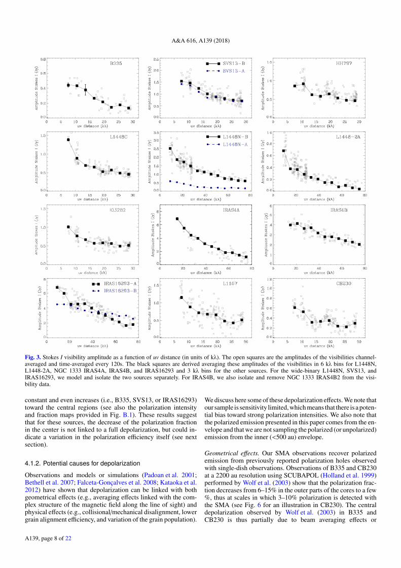
Table 6. Misalignment between the outflow angles χo and the meanmagnetic field orientation χB1000 in the central 1000 au.

Name χao χB1000 | χo–χB1000 |

() ()

B335 90 55±3 35SVS13-A 148 140±3 8SVS13-B 160 19±6 39HH797 150 113±2 37L1448C 161 – –L1448N-B 105 23±5 82L1448-2A 138 – –IRAS03282 120 – –NGC 1333 IRAS4A 170 57±13 67NGC 1333 IRAS4B 0 58±49 58IRAS16293-A 145 163±15 18IRAS16293-B 130 114±17 16L1157 146 146±4 0CB230 172 86±3 86

Notes. (a) Position angles are provided east of north.References. Bachiller et al. (1998), Bachiller et al. (2001), Choi(2001), Hull et al. (2013), Hull et al. (2014), Rodríguez et al. (1997),Tafalla et al. (2006), Rao et al. (2009), Santangelo et al. (2015), andYen et al. (2015).

Fig. 8. Histogram of the projected angles between the magnetic fieldand outflow direction. The data share a common synthesized beam sizeof about 5.5′′ and are binned with pixels of 1.8′′ for this analysis.The top panel shows the histogram color-coded per source while thebottom panel shows the global histogram (in white) with the histogramrestricted to detections within the central 1500 au overlaid in gray.

at the envelope scales traced by the SMA can be affected by thestrong rotational energy in the envelope. These results are con-sistent with predictions from numerical simulations that showa strong relation between the angular velocity of the envelopeand magnetic field direction (Machida et al. 2005, 2007). Rota-tionally twisted magnetic fields have already been observed atlarger scales (Girart et al. 2013; Qiu et al. 2013). After a givennumber of periods, rotation could be distorting or even twistingthe field lines, producing a toroidal component in the equato-rial plane. Using MHD simulations, Ciardi & Hennebelle (2010)and Joos et al. (2012) showed that the mass ejection via outflowsis less efficient when the rotation axis and B direction are mis-aligned and that outflows could be less efficient when the rotationaxis and B direction are misaligned. The presence of outflowsin sources withAB−O ∼ 90 might favor a twisted/pinched mag-netic field scenario compared to an initially misaligned magneticfield configuration.

Reinforcing the possible correlation between the field mis-alignment and the presence of strong rotational motions, ourSMA observations also suggest that a possible correlationcould be present between the envelope-scale main magneticfield direction and the multiplicity observed in the inner en-velopes. Indeed, sources that present a strong misalignment(IRAS03282, NGC 1333 IRAS4A, L1448N, L1448-2A, orCB230) are all close multiples (Maury et al., in prep.; Launhardt2004; Chandler et al. 2005; Choi 2005; Tobin et al. 2013, 2016).SVS13-A does host a close multiple but it is a Class I. We arethus not witnessing the initial conditions leading to fragmenta-tion, and the magnetic field we observe could have been severelyaffected by the evolution of both the environment and the pro-tostar itself. On the contrary, sources that show an alignmentbetween the B direction and the outflow direction (e.g., L1157,B335, SVS13-B, and L1448C) have been studied with ALMAor the NOrthern Extended Millimeter Array (NOEMA) high-resolution observations and stand as robust single protostars atenvelope scales of ∼5000–10000 au. No large disk has been de-tected so far in these sources (Saito et al. 1999; Yen et al. 2010;Chiang et al. 2012; Tobin et al. 2015) while L1448N-B for in-stance was suggested recently to harbor a large disk encom-passing several multiple sources at scales ∼100 au (Tobin et al.2016). These results support those of Zhang et al. (2014): thepossible link between fragmentation and magnetic field topologypoints toward a less efficient magnetic braking and redistributionof angular momentum when the B-field is misaligned.

5. Summary

We perform a survey of 0.87 mm continuum and polarized emis-sion from dust toward 12 low-mass Class 0 protostars.

(i) By comparing the 0.87 mm SMA continuum fluxes withsingle-dish observations, we find that our interferometric obser-vations recover <20% of the total fluxes. The fluxes derived di-rectly from the visibility data are also about twice larger thanthose derived on the reconstructed maps. For five objects, weobserved baselines above 40 kλ that allow us to separate themost compact components. The low flux fractions contained inthe compact component are consistent with the classification asClass 0 of our sources.(ii) We report the detection of linearly polarized dust emissionin all the objects of the sample with mean polarization fractionsranging from 2% to 10%.(iii) We find a decrease of the polarization fraction with the esti-mated H2 column density. Our polarization intensity profiles are

A139, page 13 of 22

A&A 616, A139 (2018)

relatively flat in most of our sources and increases toward thecenter in B335, SVS13, or IRAS16293, suggesting a decreasein the dust alignment efficiency rather than a polarization can-cellation in these sources. Two-lobe structures in the polarizedintensity distributions are observed in NGC 1333 IRAS4A andIRAS4B.(iv) The orientations observed at 0.87 mm with SMA and 1.3 mmwith CARMA are consistent with each other on the 1000 auscales probed in this analysis.(v) As in Hull et al. (2013), we find that sources with a high po-larization fraction have consistent large-to-small-scale fields. Wedo not observe, however, a relation between the misalignment ofthe magnetic field orientation with respect to the outflow axisand the polarization intensity or fraction.(vi) We find clues that large misalignment of the magnetic fieldorientation with the outflow orientation could be found preferen-tially in protostars with a higher rotational energy. The misalign-ment of 90 observed in some objects could thus be a signature ofwinding of the magnetic field lines in the equatorial plane whenthe rotational energy is significant. Strengthening this possiblelink, there are also hints that a B-outflow misalignment is foundpreferentially in protostars that are close multiple and/or harbora larger disk, while single objects seem to show a good agree-ment between the magnetic field direction at envelope scales andthe direction of their protostellar outflow. This suggests that thetopology and strength of magnetic fields at envelope scale maysignificantly impact the outcome of protostellar collapse, even-tually playing a major role in the formation of disks and multiplesystems.

Our results are aligned with previous studies of B in massivecores (Zhang et al. 2014) as well as with theoretical predictionsfrom magnetic collapse models (Machida et al. 2005; Joos et al.2012). More observations of the magnetic field of low-mass pro-tostars at envelope scale would be necessary to observationallyconfirm these tentative, but promising results and reinforce ourinterpretations.

Acknowledgements. We thank Baobab Liu for fruitful discussions on thisproject and Bilal Ladjelate for providing the internal luminosities from theHerschel Gould Belt Survey dataset for the sources belonging to the CALYPSOsample. This project has received funding from the European Research Council(ERC) under the European Union Horizon 2020 research and innovation pro-gram (MagneticYSOs project, grant agreement N 679937). JMG is supportedby the MINECO (Spain) AYA2014-57369-C3 and AYA2017-84390-C2 grants.SPL acknowledges support from the Ministry of Science and Technology of Tai-wan with Grant MOST 106-2119-M-007-021-MY3. This publication is basedon data of the Submillimeter Array. The SMA is a joint project between theSmithsonian Astrophysical Observatory and the Academia Sinica Institute of As-tronomy and Astrophysics, and is funded by the Smithsonian Institution and theAcademia Sinica.

ReferencesAlves, F. O., Frau, P., Girart, J. M., et al. 2014, A&A, 569, L1Andersson, B.-G., Lazarian, A., & Vaillancourt, J. E. 2015, ARA&A, 53, 501Andre, P., Ward-Thompson, D., & Barsony, M. 1993, ApJ, 406, 122Andre, P., Ward-Thompson, D., & Barsony, M. 2000, Protostars and Planets IV,

59Attard, M., Houde, M., Novak, G., et al. 2009, ApJ, 702, 1584Bachiller, R., Martin-Pintado, J., & Planesas, P. 1991, A&A, 251, 639Bachiller, R., Guilloteau, S., Dutrey, A., Planesas, P., & Martin-Pintado, J. 1995,

A&A, 299, 857Bachiller, R., Guilloteau, S., Gueth, F., et al. 1998, A&A, 339, L49Bachiller, R., Gueth, F., Guilloteau, S., Tafalla, M., & Dutrey, A. 2000, A&A,

362, L33Bachiller, R., Pérez Gutiérrez, M., Kumar, M. S. N., & Tafalla, M. 2001, A&A,

372, 899Bally, J. 2016, ARA&A, 54, 491

Barsony, M., Ward-Thompson, D., André, P., & O’Linger, J. 1998, ApJ, 509,733

Belloche, A. 2013, in EAS Pub. Ser., eds. P. Hennebelle, & C. Charbonnel, 62,25

Belloche, A., Hennebelle, P., & André, P. 2006, A&A, 453, 145Bertrang, G., Wolf, S., & Das, H. S. 2014, A&A, 565, A94Bethell, T. J., Chepurnov, A., Lazarian, A., & Kim, J. 2007, ApJ, 663, 1055Bock, D. C.-J., Bolatto, A. D., Hawkins, D. W., et al. 2006, Proc. SPIE, 6267,

626713Bodenheimer, P. 1995, ARA&A, 33, 199Bontemps, S., Andre, P., Terebey, S., & Cabrit, S. 1996, A&A, 311, 858Brauer, R., Wolf, S., & Reissl, S. 2016, A&A, 588, A129Caselli, P., Benson, P. J., Myers, P. C., & Tafalla, M. 2002, ApJ, 572, 238Chacón-Tanarro, A., Caselli, P., Bizzocchi, L., et al. 2017, A&A, 606, A142Chandler, C. J., & Richer, J. S. 2000, ApJ, 530, 851Chandler, C. J., Brogan, C. L., Shirley, Y. L., & Loinard, L. 2005, ApJ, 632, 371Chapman, N. L., Davidson, J. A., Goldsmith, P. F., et al. 2013, ApJ, 770, 151Chen, X., Launhardt, R., & Henning, T. 2007, ApJ, 669, 1058Chen, X., Launhardt, R., & Henning, T. 2009, ApJ, 691, 1729Chen, X., Arce, H. G., Zhang, Q., et al. 2013, ApJ, 768, 110Chiang, H.-F., Looney, L. W., & Tobin, J. J. 2012, ApJ, 756, 168Ching, T.-C., Lai, S.-P., Zhang, Q., et al. 2016, ApJ, 819, 159Choi, M. 2001, ApJ, 553, 219Choi, M. 2005, ApJ, 630, 976Ciardi, A., & Hennebelle, P. 2010, MNRAS, 409, L39Ciardi, D. R., Telesco, C. M., Williams, J. P., et al. 2003, ApJ, 585, 392Correia, J. C., Griffin, M., & Saraceno, P. 2004, A&A, 418, 607Crimier, N., Ceccarelli, C., Maret, S., et al. 2010, A&A, 519, A65Crutcher, R. M. 2012, ARA&A, 50, 29Crutcher, R. M., Nutter, D. J., Ward-Thompson, D., & Kirk, J. M. 2004, ApJ,

600, 279Curiel, S., Raymond, J. C., Moran, J. M., Rodriguez, L. F., & Canto, J. 1990,

ApJ, 365, L85Curiel, S., Torrelles, J. M., Rodríguez, L. F., Gómez, J. F., & Anglada, G. 1999,

ApJ, 527, 310Curran, R. L., & Chrysostomou, A. 2007, MNRAS, 382, 699Davidson, J. A., Novak, G., Matthews, T. G., et al. 2011, ApJ, 732, 97Di Francesco, J., Myers, P. C., Wilner, D. J., Ohashi, N., & Mardones, D. 2001,

ApJ, 562, 770Di Francesco, J., Johnstone, D., Kirk, H., MacKenzie, T., & Ledwosinska, E.

2008, ApJS, 175, 277Dotson, J. L. 1996, ApJ, 470, 566Enoch, M. L., Corder, S., Duchêne, G., et al. 2011, ApJS, 195, 21Evans, II, N. J., Dunham, M. M., Jørgensen, J. K., et al. 2009, ApJS, 181, 321Evans, II, N. J., Di Francesco, J., Lee, J.-E., et al. 2015, ApJ, 814, 22Falceta-Gonçalves, D., Lazarian, A., & Kowal, G. 2008, ApJ, 679, 537Frau, P., Galli, D., & Girart, J. M. 2011, A&A, 535, A44Gâlfalk, M., & Olofsson, G. 2007, A&A, 475, 281Galli, D., Lizano, S., Shu, F. H., & Allen, A. 2006, ApJ, 647, 374Girart, J. M., Crutcher, R. M., & Rao, R. 1999, ApJ, 525, L109Girart, J. M., Rao, R., & Marrone, D. P. 2006, Science, 313, 812Girart, J. M., Frau, P., Zhang, Q., et al. 2013, ApJ, 772, 69Girart, J. M., Estalella, R., Palau, A., Torrelles, J. M., & Rao, R. 2014, ApJ, 780,

L11Gonçalves, J., Galli, D., & Girart, J. M. 2008, A&A, 490, L39Goodman, A. A., Benson, P. J., Fuller, G. A., & Myers, P. C. 1993, ApJ, 406,

528Gueth, F., Guilloteau, S., & Bachiller, R. 1996, A&A, 307, 891Harvey, D. W. A., Wilner, D. J., Myers, P. C., & Tafalla, M. 2003, ApJ, 596, 383Hennebelle, P., & Ciardi, A. 2009, A&A, 506, L29Henning, T., Wolf, S., Launhardt, R., & Waters, R. 2001, ApJ, 561, 871Hildebrand, R. H. 1983, QJRAS, 24, 267Hirano, N., Kameya, O., Nakayama, M., & Takakubo, K. 1988, ApJ, 327, L69Hirano, N., Ho, P. P. T., Liu, S.-Y., et al. 2010, ApJ, 717, 58Hirota, T., Bushimata, T., Choi, Y. K., et al. 2008, PASJ, 60, 37Hirota, T., Honma, M., Imai, H., et al. 2011, PASJ, 63, 1Ho, P. T. P., Moran, J. M., & Lo, K. Y. 2004, ApJ, 616, L1Hoang, T., & Lazarian, A. 2009, ApJ, 695, 1457Holland, W. S., Robson, E. I., Gear, W. K., et al. 1999, MNRAS, 303, 659Hull, C. L. H., Plambeck, R. L., Bolatto, A. D., et al. 2013, ApJ, 768, 159Hull, C. L. H., Plambeck, R. L., Kwon, W., et al. 2014, ApJS, 213, 13Hull, C. L. H., Girart, J. M., Tychoniec, Ł., et al. 2017, ApJ, 847, 92Jennings, R. E., Cameron, D. H. M., Cudlip, W., & Hirst, C. J. 1987, MNRAS,

226, 461Jones, T. J., Bagley, M., Krejny, M., Andersson, B.-G., & Bastien, P. 2015, AJ,

149, 31Jones, T. J., Gordon, M., Shenoy, D., et al. 2016, AJ, 151, 156Joos, M., Hennebelle, P., & Ciardi, A. 2012, A&A, 543, A128

A139, page 14 of 22

M. Galametz et al: Polarized dust emission in solar-type Class 0 protostars

Jørgensen, J. K., Harvey, P. M., Evans, II, N. J., et al. 2006, ApJ, 645, 1246Jørgensen, J. K., Bourke, T. L., Myers, P. C., et al. 2007, ApJ, 659, 479Jørgensen, J. K., van der Wiel, M. H. D., Coutens, A., et al. 2016, A&A, 595,

A117Kataoka, A., Machida, M. N., & Tomisaka, K. 2012, ApJ, 761, 40Kataoka, A., Muto, T., Momose, M., et al. 2015, ApJ, 809, 78Kauffmann, J., Bertoldi, F., Bourke, T. L., Evans, II, N. J., & Lee, C. W. 2008,

A&A, 487, 993Keene, J., Davidson, J. A., Harper, D. A., et al. 1983, ApJ, 274, L43Knude, J., & Hog, E. 1998, A&A, 338, 897Koumpia, E., van der Tak, F. F. S., Kwon, W., et al. 2016, A&A, 595, A51Krumholz, M. R., Crutcher, R. M., & Hull, C. L. H. 2013, ApJ, 767, L11Kwon, W., Looney, L. W., Crutcher, R. M., & Kirk, J. M. 2006, ApJ, 653, 1358Kwon, W., Looney, L. W., Mundy, L. G., Chiang, H.-F., & Kemball, A. J. 2009,

ApJ, 696, 841Kwon, W., Fernández-López, M., Stephens, I. W., & Looney, L. W. 2015, ApJ,

814, 43Lai, S.-P., Crutcher, R. M., Girart, J. M., & Rao, R. 2002, ApJ, 566, 925Launhardt, R. 2001, in IAU Symp., The Formation of Binary Stars, eds.

H. Zinnecker, & R. Mathieu, 200, 117Launhardt, R. 2004, in IAU Symp., Star Formation at High Angular Resolution,

eds. M. G. Burton, R. Jayawardhana, & T. L. Bourke, 221, 213Launhardt, R., Stutz, A. M., Schmiedeke, A., et al. 2013, A&A, 551, A98Lazarian, A. 2007, J. Quant. Spectr. Rad. Transf., 106, 225Lee, K. I., Dunham, M. M., Myers, P. C., et al. 2015, ApJ, 814, 114Lee, J. W. Y., Hull, C. L. H., & Offner, S. S. R. 2017, ApJ, 834, 201Lefloch, B., Castets, A., Cernicharo, J., Langer, W. D., & Zylka, R. 1998, A&A,

334, 269Li, Z.-Y., Krasnopolsky, R., & Shang, H. 2013, ApJ, 774, 82Li, H.-B., Goodman, A., Sridharan, T. K., et al. 2014, Protostars and Planets VI,

101Liu, H. B., Lai, S.-P., Hasegawa, Y., et al. 2016, ApJ, 821, 41Loinard, L., Zapata, L. A., Rodríguez, L. F., et al. 2013, MNRAS, 430, L10Looney, L. W., Mundy, L. G., & Welch, W. J. 2000, ApJ, 529, 477Looney, L. W., Mundy, L. G., & Welch, W. J. 2003, ApJ, 592, 255Looney, L. W., Tobin, J. J., & Kwon, W. 2007, ApJ, 670, L131López-Sepulcre, A., Sakai, N., Neri, R., et al. 2017, A&A, 606, A121Machida, M. N., Matsumoto, T., Tomisaka, K., & Hanawa, T. 2005, MNRAS,

362, 369Machida, M. N., Inutsuka, S.-i., & Matsumoto, T. 2007, ApJ, 670, 1198Marrone, D. P. 2006, PhD thesis, Harvard UniversityMarrone, D. P., & Rao, R. 2008, in Proc. SPIE, Millimeter and Submillimeter

Detectors and Instrumentation for Astronomy IV, 7020, 70202BMarvel, K. B., Wilking, B. A., Claussen, M. J., & Wootten, A. 2008, ApJ, 685,

285Massi, F., Codella, C., Brand, J., di Fabrizio, L., & Wouterloot, J. G. A. 2008,

A&A, 490, 1079Matthews, B. C., & Wilson, C. D. 2000, ApJ, 531, 868Matthews, B. C., McPhee, C. A., Fissel, L. M., & Curran, R. L. 2009, ApJS, 182,

143Maury, A. J., André, P., Hennebelle, P., et al. 2010, A&A, 512, A40Maury, A. J., André, P., Men’shchikov, A., Könyves, V., & Bontemps, S. 2011,

A&A, 535, A77Maury, A. J., Belloche, A., André, P., et al. 2014, A&A, 563, L2Maury, A. J., Girart, J. M., Zhang, Q., et al. 2018, MNRAS, 477, 2760Motte, F., & André, P. 2001, A&A, 365, 440Ohashi, N., Saigo, K., Aso, Y., et al. 2014, ApJ, 796, 131O’Linger, J., Wolf-Chase, G., Barsony, M., & Ward-Thompson, D. 1999, ApJ,

515, 696Ossenkopf, V., & Henning, T. 1994, A&A, 291, 943Oya, Y., Sakai, N., López-Sepulcre, A., et al. 2016, ApJ, 824, 88

Padoan, P., Goodman, A., Draine, B. T., et al. 2001, ApJ, 559, 1005Palau, A., Zapata, L. A., Rodríguez, L. F., et al. 2014, MNRAS, 444, 833Pech, G., Zapata, L. A., Loinard, L., & Rodríguez, L. F. 2012, ApJ, 751, 78Pelkonen, V.-M., Juvela, M., & Padoan, P. 2009, A&A, 502, 833Pineda, J. E., Maury, A. J., Fuller, G. A., et al. 2012, A&A, 544, L7Planck Collaboration Int. XXXV. 2016, A&A, 586, A138Plunkett, A. L., Arce, H. G., Corder, S. A., et al. 2013, ApJ, 774, 22Podio, L., Codella, C., Gueth, F., et al. 2016, A&A, 593, L4Poidevin, F., Bastien, P., & Matthews, B. C. 2010, ApJ, 716, 893Pudritz, R. E., & Norman, C. A. 1983, ApJ, 274, 677Qiu, K., Zhang, Q., Menten, K. M., Liu, H. B., & Tang, Y.-W. 2013, ApJ, 779,

182Rao, R., Crutcher, R. M., Plambeck, R. L., & Wright, M. C. H. 1998, ApJ, 502,

L75Rao, R., Girart, J. M., Marrone, D. P., Lai, S.-P., & Schnee, S. 2009, ApJ, 707,

921Reipurth, B., Heathcote, S., & Vrba, F. 1992, A&A, 256, 225Reipurth, B., Rodríguez, L. F., Anglada, G., & Bally, J. 2002, AJ, 124, 1045Rodríguez, L. F., Anglada, G., & Curiel, S. 1997, ApJ, 480, L125Sadavoy, S. I., Di Francesco, J., Andre, P., et al. 2014, ApJ, 787, L18Saito, M., Sunada, K., Kawabe, R., Kitamura, Y., & Hirano, N. 1999, ApJ, 518,

334Santangelo, G., Codella, C., Cabrit, S., et al. 2015, A&A, 584, A126Schuller, F., Menten, K. M., Contreras, Y., et al. 2009, A&A, 504, 415Segura-Cox, D. M., Looney, L. W., Stephens, I. W., et al. 2015, ApJ, 798, L2Segura-Cox, D. M., Harris, R. J., Tobin, J. J., et al. 2016, ApJ, 817, L14Seifried, D., Banerjee, R., Pudritz, R. E., & Klessen, R. S. 2015, MNRAS, 446,

2776Shu, F. H., Najita, J. R., Shang, H., & Li, Z.-Y. 2000, Protostars and Planets IV,

789Stephens, I. W., Looney, L. W., Kwon, W., et al. 2013, ApJ, 769, L15Straizys, V., Cernis, K., Kazlauskas, A., & Meistas, E. 1992, Balt. Astron., 1,

149Stutz, A. M., Rubin, M., Werner, M. W., et al. 2008, ApJ, 687, 389Tafalla, M., & Bachiller, R. 1995, ApJ, 443, L37Tafalla, M., Kumar, M. S. N., & Bachiller, R. 2006, A&A, 456, 179Tang, Y.-W., Ho, P. T. P., Koch, P. M., Guilloteau, S., & Dutrey, A. 2013, ApJ,

763, 135Terebey, S., Chandler, C. J., & Andre, P. 1993, ApJ, 414, 759Terebey, S., & Padgett, D. L. 1997, in IAU Symp., Herbig-Haro Flows and the

Birth of Stars, eds. B. Reipurth, & C. Bertout, 182, 507Tobin, J. J., Looney, L. W., Mundy, L. G., Kwon, W., & Hamidouche, M. 2007,

ApJ, 659, 1404Tobin, J. J., Hartmann, L., Chiang, H.-F., et al. 2011, ApJ, 740, 45Tobin, J. J., Chandler, C. J., Wilner, D. J., et al. 2013, ApJ, 779, 93Tobin, J. J., Looney, L. W., Wilner, D. J., et al. 2015, ApJ, 805, 125Tobin, J. J., Looney, L. W., Li, Z.-Y., et al. 2016, ApJ, 818, 73Watson, D. M., Bohac, C. J., Hull, C., et al. 2007, Nature, 448, 1026Welch, W. J., Thornton, D. D., Plambeck, R. L., et al. 1996, PASP, 108, 93Whittet, D. C. B., Hough, J. H., Lazarian, A., & Hoang, T. 2008, ApJ, 674, 304Wolf, S., Launhardt, R., & Henning, T. 2003, ApJ, 592, 233Wolf-Chase, G. A., Barsony, M., & O’Linger, J. 2000, aj, 120, 1467Wu, J., Dunham, M. M., Evans, II, N. J., Bourke, T. L., & Young, C. H. 2007,

AJ, 133, 1560Yeh, S. C. C., Hirano, N., Bourke, T. L., et al. 2008, ApJ, 675, 454Yen, H.-W., Takakuwa, S., & Ohashi, N. 2010, ApJ, 710, 1786Yen, H.-W., Takakuwa, S., & Ohashi, N. 2011, ApJ, 742, 57Yen, H.-W., Takakuwa, S., Ohashi, N., & Ho, P. T. P. 2013, ApJ, 772, 22Yen, H.-W., Koch, P. M., Takakuwa, S., et al. 2015, ApJ, 799, 193Zhang, Q., Ho, P. T. P., Wright, M. C. H., & Wilner, D. J. 1995, ApJ, 451, L71Zhang, Q., Qiu, K., Girart, J. M., et al. 2014, ApJ, 792, 116

A139, page 15 of 22

A&A 616, A139 (2018)

Appendix A: Source description

In this section, we provide a quick description of the objects andof the 0.87 mm continuum observed with the SMA.

B335B335 is an isolated Bok globule hosting a Class 0 protostar. Itsluminosity is ∼1 LM (Keene et al. 1983) and its mass < 2MM .Ouflows. It possesses an east-west elongated, conical-shapedmolecular outflow (PA: 80; Hirano et al. 1988). Collimated12CO (2−1) jets (Yen et al. 2010) and Herbig-Haro (HH) objects(HH 119 A−F; Reipurth et al. 1992; Gâlfalk & Olofsson 2007)are detected along this outflow axis.Velocity field. C18O (2−1) and H13CO+ (1−0) interferometricobservations have traced the rotational infalling motion of theenvelope from radii of ∼20 000 down to ∼1000 au. No clear rota-tional motion is detected on 100–500 au scales (Saito et al. 1999;Harvey et al. 2003; Yen et al. 2011) and the central circumstellardisk radius is estimated to be smaller than 100 au.Our SMA observations. The SMA 0.87 mm continuum emissionhas a north-south elongated structure coherent with previous 1.3mm observations of the object by Motte & André (2001). Thetwo protuberances observed in the north and southwest regionstrace the edge of the cavity produced by the horizontal outflow(Yen et al. 2010).

SVS13SVS13 is a multiple system in the NGC 1333 star-forming re-gion. It possesses three main submillimeter continuum sourcesaligned in the northeast-southwest direction named A, B, andC (Looney et al. 2003). SVS13-A is a Class I protostar whileSVS13-B and C are Class 0. A large filamentary structure en-compasses the three sources at 450 µm (Chandler & Richer2000) and at millimeter wavelengths (Hull et al. 2014). Thecombined luminosity for SVS13-A, B, and C is 45 LM(Jennings et al. 1987). Emission at 70 µmis detected towardSVS13-A and C but not toward SVS13-B, suggesting that thesource is deeply embedded (Chen et al. 2009). A radio sourcecalled VLA3 has also been detected southwest of SVS13-A(Rodríguez et al. 1997).Ouflows. SVS13-A is likely powering the strong northwest-southeast HH7-11 outflow studied by Bachiller et al. (2000) andPlunkett et al. (2013). SVS13-B is known to drive a highly col-limated SiO jet (Bachiller et al. 1998).Velocity field. A symmetric velocity gradient of 28 km s−1 pc−1

across SVS13-B and SVS13A/VLA3 has been detected usingN2H+ observations. This large gradient could suggest that thewide binary system is physically bound (Chen et al. 2009).Our SMA observations. The SMA 0.87 mm observations tracethe extended envelope around SVS13-A and SVS13-B. We re-solve the two sources while SVS13-C is only marginally de-tected in the southwest. The continuum emission of SVS13-Ais slightly elongated in the southwest direction toward the posi-tion of VLA3. The 0.87 mm emission of SVS13-B extends inthe north-northwest direction. That extension aligns with that ofthe SiO jet driven by the protostar. The continuum emission alsoextends in the southwest direction of SVS13-B. The extension isalso observed in the elongated N2H+ map but not in the PdBI 1.4mm and 3 mm observations, which could be linked with filteringeffects affecting the PdBI maps (Chen et al. 2009).

IC348-SMM2 / HH797SMM2 is a low-mass class 0 belonging to the IC 348 star-forming region. The SMA observations also reveal a compan-ion source, SMM2E, at ∼2400 au in the northeast direction

(Palau et al. 2014) whose spectral energy distribution is typicalof Class 0 objects.Ouflows. SMM2 probably drives the HH797 jet, which hasa very extended and collimated northwest-southeast outflow(Chen et al. 2013). Velocity asymmetries along the length ofthe flow were interpreted as jet rotation (Pech et al. 2012). Acompact low-velocity outflow also seems to be associated withSMM2E.Velocity field. C18O observations of the companion sourceSMM2E suggest that the envelope is probably rotating witha north-south axis close to the outflow direction (Palau et al.2014).Our SMA observations. Our 0.87 mm continuum map is con-sistent with that previously obtained by Palau et al. (2014) withSMA as well as far-IR continuum emission observed with Her-schel. Both SMM2 and SMM2E are detected at 0.87 mm, butSMME2 is not resolved.

L1448CThe L1448C complex (also called L1448-mm) hosts several em-bedded Class 0 protostars (Tobin et al. 2007).Ouflows. It possesses well-collimated outflows (Hirano et al.2010). The northern CO lobe is probably interacting with theneighboring source L1448N (Bachiller et al. 1995).Velocity field. VLA observations of NH3 reveal velocity gradi-ents perpendicular to the outflow as well as along the outflowaxis. This suggests the presence of a self-gravitating structurearound L1448C, which has an envelope that is both rotating andcontracting at comparable velocities (Curiel et al. 1999).Our SMA observations. Our SMA observations show thatL1448C is elongated in the northwest-southeast direction,which is consistent with the elongation observed at 1.3 mm(Barsony et al. 1998). The southeast elongation encompassesthe companion source L1448-mm B (2000 au separation) ob-served with Spitzer (Tobin et al. 2007) (also called L1448C(S);Jørgensen et al. 2006). A distortion is also observed in the south-west direction, where a 0.80 mm continuum emission has beenobserved by Barsony et al. (1998). This distortion and the north-ern elongation could also be tracing the edge of the outflowcavities.

L1448NL1448N (or L1448 IRS3) is a multiple system. L1448N-Ais located 2100 au north to L1448N-B. B is the strongestsource at millimeter wavelengths (Looney et al. 2000) whileA dominates at mid-infrared (Ciardi et al. 2003) and centime-ter wavelengths (Curiel et al. 1990). The system is also con-nected to L1448NW located 20′′ north. Barsony et al. (1998)suggested that star formation in L1448N could have beeninduced by the strong outflow driven by L1448C (see alsoKwon et al. 2006).Ouflows. Two bipolar outflows originate from the system. Theoutflow driven by L1448N-A is nearly perpendicular to the lineof sight. Kwon et al. (2006) showed that the two outflows areprobably interacting with each other.Velocity field. The inner 5–10′′ of L1448N presents a solid-body rotation while the outer envelope shows a flatter pro-file (Terebey & Padgett 1997). C18O observations also reveal astrong velocity gradient (>100 km s−1 pc−1; Gaudel et al., inprep.; Yen et al. 2015) perpendicular to the outflow directionwithin 20 (Lee et al. 2015).Our SMA observations. L1448N-A and B are resolved by theSMA while L1448NW is marginally detected. Both sources areelongated in the northeast-southwest direction, which is consis-

A139, page 16 of 22

M. Galametz et al: Polarized dust emission in solar-type Class 0 protostars

tent with previous 230 GHz and 0.87 mm SMA observations byLee et al. (2015).

L1448-2AL1448-2A (or L1448 IRS 2) is a low luminosity (5.2 L) Class 0protostar located toward the western edge of the L1448 complexthat seems to be evolving in isolation from L1448N and C.Ouflows. High-velocity CO maps show that L1448-2A drivesan outflow in the northwest-southeast direction (O’Linger et al.1999). Additional studies from Wolf-Chase et al. (2000) sug-gested that the source is actually driving two distinct outflows,which could be a signature of an unresolved binary system.Velocity field. Using C18O observations, Yen et al. (2015) founda velocity gradient nearly perpendicular to the outflow axis.Our SMA observations. The northeast-southwest extensionof the envelope is confirmed by our SMA observation.Contrary to the CARMA 1.3 mm dust continuum pre-sented in Hull et al. (2014), we do not observe elon-gation in the northwest-southeast direction. As thiselongation is not observed at other wavelengths, we con-clude that the elongation observed at 1.3 mm might be due tocontamination by the outflow. The horns detected in the east andwest direction trace the edges of the large outflow cavity.

IRAS03282IRAS03282 is a highly embedded Class 0 object lying at 1southeast of NGC 1333 (Jørgensen et al. 2006). IRAS 03282possesses two sources separated by 1.5′′ (Launhardt 2004).Outflows. The source drives an outflow in which various velocitycomponents are observed, in particular a high-velocity(∼60 km s−1) jet with fast molecular clumps detected along theoutflow axis surrounded by a less collimated and more standardvelocity (∼20 km s−1) outflow (Bachiller et al. 1991).Velocity field. N2H+ and NH3 observations were used to trace thelarge-scale velocity gradient of the envelope that is mostly dis-tributed along the outflow direction (Tobin et al. 2011).Our SMA observations. The N2H+ and NH3 maps present anelongation along the north-south direction. Our SMA 0.87 mmmap presents a similar elongation. The southern elongation isalso very similar to that observed at 350 µm by Wu et al. (2007)with SHARC-II.

NGC 1333 IRAS4ANGC 1333 IRAS4A is a Class 0 object located in the south ofNGC 1333. It hosts two sources (IRAS4A1 and IRAS4A2) ina close (1.8′′) binary pair that was resolved with interferome-ters at submillimeter and millimeter wavelengths using the SMAor BIMA (Looney et al. 2000; Girart et al. 2006; Jørgensen et al.2007) and more recently ALMA (López-Sepulcre et al. 2017):IRAS4A1 dominates the submillimeter and millimeter emission.Outflows. An arcmin-long outflow, seen in high-velocity CO(3-2) emission, is associated with IRAS4A2 and bends from anorth-south orientation on small scales (Santangelo et al. 2015)to a position angle of 45 on large scales Koumpia et al. (2016).This could be due to an intrinsic change of the gas propagationdirection or a signature of jet precession. The launching direc-tion of the outflow driven by IRAS4A1 is also oriented close tonorth-south direction and faster (Santangelo et al. 2015). Part ofthat SiO outflow (position angle of -10) was also reported byChoi (2001).Velocity field. Detections of inverse P-Cygni profiles in thelines of common molecular species such as 13CO or CSare interpreted as signs of strong infall motions of theouter cloud (Di Francesco et al. 2001; Jørgensen et al. 2007).Belloche et al. (2006) detected a centroid velocity gradient ofabout 10 km s −1 pc−1, with a position angle of 38, while

Ching et al. (2016) found a velocity gradient along the axis link-ing NGC 1333 IRAS4A1 and IRAS4A2. Both Belloche et al.(2006) and Gaudel et al (in prep.) showed however that the in-terpretation of these velocity gradients in terms of rotation is notstraightforward in IRAS4A owing to the strong infall motionspreviously mentioned.Our SMA observations. As already shown in Girart et al. (2006),the SMA 0.87 mm map presents a very compact structure ex-tended in the A1-A2 direction. The common envelope extendsin the northeast and southwest direction, in the same direction(∼30–50) as i) the velocity gradient found in Belloche et al.(2006), ii) the outflow takes further from the protostar, andiii) that the large-scale B orientation observed by SCUBA(Matthews et al. 2009).

NGC 1333 IRAS4BNGC 1333 IRAS4B is also a Class 0 protostar and be-longs to the same N2H+ arcmin-scale filament asIRAS4A. Submillimeter and millimeter observations re-veal a second source located 11′′ on the east (IRAS4B2)(Looney et al. 2000). IRAS4B2 is not detected atcentimeter wavelengths, suggesting that it is at a differentstage of its evolution (Reipurth et al. 2002) or just not associatedat all with IRAS4B. There is still some debate on smaller scaleson whether the disk of IRAS 4B is observed face- or edge-on(Watson et al. 2007; Marvel et al. 2008).Outflows. The source is driving an outflow whose axis is nearlyin north-south direction. Its short dynamical timescale suggeststhat this outflow is very young (Choi 2001).Velocity field. IRAS4B seems to be collapsing (Di Francesco et al.2001; Belloche et al. 2006) but does not show clear signs ofrotational motions at 1000 au scales (Yen et al. 2013).Our SMA observations. The SMA 0.87 mm map of IRAS4Bpresents a very compact structure that seems to be extendedin the north-south direction, namely the direction of the out-flow emanating from this source. We do not observe the sameeast-west extension as seen at 1.3 mm by Hull et al. (2014) andYen et al. (2013).

IRAS16293IRAS16293 is a Class 0 protostar system located in the ρOphiuchi molecular cloud. It possesses a bolometric luminos-ity of ∼25 LM and a massive envelope (Correia et al. 2004;Crimier et al. 2010) surrounding two cores separated by 6′′,called A (south) and B (north). Crimier et al. (2010) suggestedthat IRAS16293A/B is a “separate envelope system” (followingthe classification proposed by Looney et al. 2003). IRAS16293-A is an edge-on system and IRAS16293-B is nearly face-on(Jørgensen et al. 2016). The first dominates the system luminos-ity. The SMA observations also have enabled the separation ofIRAS16293-A into two components, Aa and Ab, aligned alonga position angle of 45 (Chandler et al. 2005). No small-scalemultiplicity has been found for IRAS16293-B.Outflows. The source shows significant outflow activity. WhileIRAS16293-A seems to be driving the main east-west CO out-flow, the driving source of the northwest-southeast compact out-flow (PA of 145) traced with SiO observations is still unclear(Yeh et al. 2008; Rao et al. 2009). This much younger outflow isprobably a more robust tracer of the rotation axis, as recent stud-ies revealed at various scales an almost edge-on rotational pat-tern whose axis match the SiO outflow orientation (Pineda et al.2012; Girart et al. 2014). A one-sided bubble-like outflowstructure originates from IRAS16293-B in the southeast direc-tion (Loinard et al. 2013).

A139, page 17 of 22

A&A 616, A139 (2018)

Velocity field. In IRAS16293-A, C34S observations reveal a clearvelocity gradient along PA 40-45, i.e., perpendicular to the SiO-traced outflow (Girart et al. 2014) probably because of the in-falling motion of the rotating envelope. A disk-like rotation isalso detected at 40–60 au with ALMA with the same orien-tation (Oya et al. 2016). In IRAS16293-B, recent ALMA ob-servations reveal inverse P-Cygni profiles toward the center ofIRAS16293-B in the CH3OCHO-A CH3OCHO-E and H2CCOlines, here again indicative of infall motions (Pineda et al. 2012).The source is observed face-on: no rotation has been detected.Our SMA observations. As shown in Rao et al. (2009), the SMA0.87 mm observations separate the two A and B components.IRAS16293-B is brighter than IRAS16293-A. The continuumemission of the envelope extends to the north of IRAS16293-Aand is also extended (∼10′′) toward its southeast direction, i.e.,in the direction of the redshifted part of the SiO outflow.

L1157L1157 is a low-mass Class 0 protostar and seems to be a singlesystem (Tobin et al. 2013).Outflows. It possesses a spectacular bipolar outflow asymmetricon large scales. Its prominent CO cavities are likely created bythe propagation of large bow shocks (also traced via the NH3or SiO molecular lines; Tafalla & Bachiller 1995; Zhang et al.1995; Gueth et al. 1996). This could be the sign that a time-variable collimated jet is driving the outflow (Podio et al. 2016).Velocity field. L1157 has a flattened and filamentary envelopepresenting a weak velocity gradient along the filament - thus per-pendicular to the outflow. Broad linewidths are observed in theinner envelope (see Kwon et al. 2015).

Our SMA observations. Our 0.87 mm observations are consistentwith those presented in Chen et al. (2013). Neither Chen et al.(2013) nor our observations detected the elongation structuredetected at 1.3 mm with Stephens et al. (2013) in the northern(outflow) direction. By contrast, we detect a similar eastern ex-tension and western bump. This horizontal elongation is also ob-served at 350 µm by Wu et al. (2007).

CB230CB 230 is an isolated globule hosting a dense core, itself host-ing two deeply embedded young stellar objects (YSOs). Theseare separated by 10′′ and are aligned in the east-west direction(Launhardt 2001, 2004). The eastern object, IRS2, is not de-tected beyond 24 µm (Massi et al. 2008; Launhardt et al. 2013).Outflows. The north-south CO outflows seem to be driven bythe western protostar IRS1. More recent 7 mm high-resolutionobservations of IRS1 led to the detection of two continuumsources separated by ∼100 au, which have an unresolved pri-mary source at the origin of the outflow and an extended com-panion source located in a direction perpendicular to the outflowdirection (Tobin et al. 2013).Velocity field. CB230 presents a velocity gradient>10 km s−1 pc−1

increasing from east to west along the axis connecting the twoembedded YSOs (Chen et al. 2007; Tobin et al. 2011). Thegradient is perpendicular to the outflow axis.Our SMA observations. The 0.87 mm continuum emission ofCB230 is elongated in a boxy-shaped structure in the north-southdirection, an elongation also observed at 1.3 mm by Hull et al.(2014). The southwest elongation could again be linked withemission tracing the edges of the north-south outflow cavity.

A139, page 18 of 22

M. Galametz et al: Polarized dust emission in solar-type Class 0 protostars

Appendix B: Stokes Q and U, polarization intensity, and fraction maps of the sample

Fig. B.1. Polarization maps of, from left to right, B335, SVS13 and HH797. Two top panels: Stokes Q and U maps. Color scales are in mJy/beam.Stokes I contours (same as in Fig. 2) appear in blue. Stokes Q and U contours appear in red and are [−3,−2,−1, 1, 2, 3] σ. Third line: polarizationintensity maps. The color scale is in mJy/beam. Fourth line: polarization fraction map. The filled ellipses on the bottom left corner indicate thesynthesized beam of the SMA maps. Same for L1448C, N and 2A. Same for IRAS03282, L1157, and CB230. Same for NGC 1333 IRAS4A,NGC 1333 IRAS4B, and IRAS16293.

A139, page 19 of 22

A&A 616, A139 (2018)

Fig. B.1. continued

A139, page 20 of 22

M. Galametz et al: Polarized dust emission in solar-type Class 0 protostars

Fig. B.1. continued

A139, page 21 of 22

A&A 616, A139 (2018)

Fig. B.1. continued

A139, page 22 of 22