Some identi–cation problems in the cointegrated vector ...sjo/papers/Dhrymes.pdf · Some identi–cation problems in the cointegrated vector autoregressive model ... cation problems

Some identi�cation problems in the cointegratedvector autoregressive model

Søren Johansen�

Department of Economics, University of Copenhagenand

CREATES, University of Aarhus

October 25, 2007

Abstract

An analysis of some identi�cation problems in the cointegrated VAR isgiven. We give a new criteria for identi�cation by linear restrictions on indi-vidual relations which is equivalent to the rank condition. We compare theasymptotic distribution of the estimators of � and �; when they are identi�edby linear restrictions on �; and when they are identi�ed by linear restrictionson �; in which case a component of � is asymptotically Gaussian. Finallywe discuss identi�cation of shocks by introducing the contemporaneous andpermanent e¤ect of a shock and the distinction between permanent and transi-tory shocks, which allows one to identify permanent shocks from the long-runvariance and transitory shocks from the short-run variance.

Keywords: Identi�cation, cointegration, common trends

JEL Classi�cation: C32

�The author wishes to thank the Danish Social Sciences Research Council for continuing sup-port.Address: Department of Economics, University of Copenhagen, Studiestræde 6, DK-1455 Copen-hagen K, Denmark. Email: [email protected]

1

2 Søren Johansen

1 Introduction

We analyze some identi�cation problems in the cointegrated vector autoregressivemodel, where it is well known that the adjustment and cointegration parametersenter through the impact matrix � = ��0:To get meaningful estimates of theseparameters we therefore need to impose identifying restrictions. The long-run im-pact matrix C is the coe¢ cient matrix of the cumulated shocks to the model andCPt

i=1 "i de�nes the common stochastic trends generated by the permanent shocks�0?"t. We discuss identi�cation of permanent shocks based upon the rows of C: Fi-nally the transitory shocks �0�1"t enter the conditional model of�Xt given �0?�Xt

and the past via the matrix B = �(�0�1�)�1�0�1and we propose to discuss iden-ti�cation of transitory shocks via the rows of B.As a result of the lack of identi�cation, the asymptotic information matrix for the

parameters (�; �) is singular, see Theorem 1. To �nd meaningful estimates we needto impose identifying restrictions on � or �, and this is usually done by restrictingthe individual cointegrating vectors by linear restrictions. We give a new criterionfor identi�cation, which is equivalent to the classical rank condition, see Lemma5, and give some applications. In Theorem 7 we give the asymptotic distributionof the identi�ed coe¢ cients when they are identi�ed by linear restrictions on �: Ifinstead we impose linear restrictions on the adjustment coe¢ cients we �nd that theasymptotic distribution of the cointegrating coe¢ cient have a Gaussian component,see Theorem 9.Finally we de�ne permanent and transitory shocks and the contemporary and

permanent e¤ects of these. If we analyze the permanent shocks by a Cholesky de-composition of the long-run variance CC 0 and the transitory shocks by a Choleskydecomposition of the short-run variance BB0; we need the asymptotic distributionof the linear combinations thus derived. These are found in Theorems 11 and 12.

2 The unrestricted cointegration model

We de�ne the cointegrated VAR model, the cointegrating relations, and the com-mons stochastic trends. We then discuss estimation of � by an eigenvalue problemand �nd the asymptotic score and information under local alternatives.

2.1 Cointegration and common trends

We consider the p�dimensional process Xt; t = 1; : : : ; T; given by the cointegrationvector autoregressive model

�Xt = ��0Xt�1 +

kXi=1

�i�Xt�i + "t; (1)

where � and � are p � r and "t are i.i.d. Np(0;): We have left out deterministicterms for simplicity. Under the assumption that the roots of the characteristic

Identification in the cointegrated VAR 3

polynomial are either outside the unit circle or equal to one, and that det(�0?(Ip �Pki=1 �i)�?) 6= 0; the solution can be represented as

Xt = CtXi=1

"i + Yt + A; (2)

where Yt is stationary and A depends on initial values, so that �0A = 0: The long-run

impact matrix matrix C is given by

C = �?(�0?(Ip �

kXi=1

�i)�?)�1�0?: (3)

It follows from (2) and (3) that the cointegrating linear combinations, �0Xt; arestationary, and the nonstationarity of Xt is generated by the common stochastictrends

St = �0?

tXi=1

"i:

We also need the conditional model for �Xt given the past and �0?�Xt; as given by

�Xt = ��0Xt�1 + !�0?�Xt +k�1Xi=1

(�i � !�0?�i)�Xt�i + "t � !�0?"t (4)

with ! = �?(�0?�?)�1; where "t � !�0?"t = B"t; and

B = Ip � �?(�0?�?)�1�0? = �(�0�1�)�1�0�1: (5)

Asymptotic inference for model (1) has been worked out, see for instance Jo-hansen (1996). In the following we give some asymptotic results without detailedproofs, but appeal to the general idea that the asymptotic distribution of the maxi-mum likelihood estimator can be found as the ratio of the limit under local alterna-tives of the score function and the information. As usual the estimators are derivedfrom the Gaussian likelihood function and their properties given under general i.i.d.errors with mean zero and �nite variance.

2.2 Estimation of the unrestricted parameters by reducedrank regression

If the parameters (�; �;�1; : : : ;�k;) are unrestricted, it is well known that theparameters can be estimated by reduced rank regression, see Anderson (1951). Weuse the Frisch-Waugh theorem to eliminate the short run dynamics �1; : : : ;�k andde�ne the residuals

R0t = (�Xtj�Xt�1; : : : ;�Xt�k) and R1t = (Xt�1j�Xt�1; : : : ;�Xt�k)

4 Søren Johansen

and the product moments Sij = T�1PT

t=1RitR0jt and S"1 = T�1

PTt=1 "tR1t: The

rest of the analysis is conducted in the pro�le likelihood function

� logLT (�; �;) = � max�1;:::;�1

logLT (�; �;�1; : : : ;�k;)

=1

2tr[�1

TXt=1

(R0t � ��0R1t)(R0t � ��0R1t)0]:

The parameter � is now estimated by solving an eigenvalue problem, and the max-imized likelihood function is used to construct tests for rank and hypotheses on �;see Johansen (1996).

2.3 Asymptotic distribution of score and information underlocal alternatives

The local experiment, see van der Vaart (1988), is constructed by �nding the limitunder local alternatives of the parameters of the score and information. We introducesome notation. Let f(x; y) be a matrix valued function of matrix arguments x and y;and let dx and dy denote directions of the same dimensions as x and y respectively.We de�ne the partial derivative of f with respect to x in the direction dx by

Dxf(x; y)(dx) = lims!0

s�1ff(x+ sdx); y)� f(x; y)g:

We use the notation fAijg for a block matrix with blocks Aij, and diagfAig for ablock diagonal matrix with diagonal blocks Ai: Finally we write A B = faijBg;and use throughout that if Z is a stochastic matrix with variance V ar(Z) = AB;then for vectors �; � we have

V ar(�0Z�) = � 0A��0B�:

We let W be the limit in distribution on Dp[0; 1] of X[Tu] = T�1=2P[Tu]

i=1 "i; andwrite

X[Tu] =) CW (u): (6)

Theorem 1 The limit in distribution of the score with respect to � in the directionT�1�?

��0?(d�) is given by

tr[�0�1Z 1

0

(dW )W 0C 0�?(��0?d�)]; (7)

which is mixed Gaussian with asymptotic conditional variance

vec(��0?d�)

0��0�1� �?C

Z 1

0

WW 0duC 0�?

�vec(��

0?d�): (8)


The score with respect to �; � in the directions T�1=2(��0(d�); (d�)0) is asymptoti-cally Gaussian with mean zero and variance

vec(��0(d�); (d�)0)0

��0�1� �0�1

�1� �1

� ��

�vec(��

0(d�); (d�)0); (9)

where �� = V ar(�0Xtj�Xt; : : : ;�Xt�k+1):The asymptotic distribution of the information is given by a block diagonal matrix

with a block corresponding to T�1�?��0?d� given by (8) and a block corresponding to

T�1=2(��0(d�); (d�)0) given by the singular matrix (9).

Proof. We let be known to simplify the calculations, and de�ne the concen-trated likelihood function lT (�; �) = �2 logLT (�; �;):We �rst �nd the score withrespect to � in the direction T�1�?��

0?(d�);

T�1D�lT (�; �)(�?�0?(d�)) = �tr[�1S"1�?��

0?(d�)�

0];

and the limits in (7) and (8) follow from (6) and

S1"d! C

Z 1

0

W (dW )0;

T�1S11d! C

Z 1

0

WW 0duC 0:

Next, the derivatives with respect to (�; �) in the directions T�1=2(��0(d�); (d�)0)are

T�1=2D�lT (�; �)(��0(d�)) = �tr[�1T 1=2S"1��

0(d�)�0]; (10)

T�1=2D�lT (�; �)(d�) = �tr[�1T 1=2S"1�(d�)0]: (11)

It follows fromT 1=2�0S1"

d! Nr�p(0; ��);

that the scores are (jointly) asymptotically Gaussian with the mean zero and vari-ance (9). The calculation of the information and its limit is given in the Appendix.

It is seen that the asymptotic distribution of the maximum likelihood estimatorscannot be derived from the results in Theorem 1 because the parameters are notidenti�ed or equivalently the asymptotic information (9) is singular. By imposingrestrictions on � or � we restrict the variation of d� and d� so that � and � becomeidenti�ed and the asymptotic information has full rank. This has the implicationthat there are cases in which � � � has a component in the direction �; so thatT 1=2(��

0(� � �); (�� )) is asymptotically Gaussian and in general correlated. This

is discussed in sections 4 and 5, but �rst we give some criteria for identi�cation bylinear restrictions.

6 Søren Johansen

3 De�nitions and criteria for identi�cation

We give here the de�nition of identi�cation and discuss some criteria for identi�ca-tion by linear restrictions on individual relations.

De�nition 2 Let fP�; � 2 �g be a family of probability measures, that is, a sta-tistical model. We say that a parameter function g(�) is identi�ed if g(�1) 6= g(�2)implies that P�1 6= P�2 ; or equivalently if P�1 = P�2 implies that g(�1) = g(�2):

In the cointegration model (1), the parameter function � = ��0 and the para-meters �1; : : : ;�k; are identi�ed, because if �

i = (�i; �i;�i1; : : : ;�ik;

i); i = 1; 2;and the (conditional) densities are equal

p(X1; : : : ; XT ; �1jX0; : : : ; X�k) = p(X1; : : : ; XT ; �

2jX0; : : : ; X�k);

then �1 = �1�10 = �2�20 = �2; �1i = �2i ; i = 1; : : : ; k; and

1 = 2: On the otherhand, given any choices of (�1; �1) and (�2; �2) for which � = �1�10 = �2�20; onecan �nd a full rank r � r matrix for which �1 = �2�0 and �1 = �2��1: Thus theidenti�cation of � and � reduces to giving such restrictions on � or �; that if � and� satisfy the restrictions and �� and ��0�1 satisfy the same restrictions, then � = Ir.A general formulation of linear restrictions on individual cointegrating relations

allows si linear restrictions the i0th vector: R0i�i = 0; i = 1; : : : ; r; where Ri is p� siof rank si. If we de�ne Hi = Ri?; then the restrictions can be formulated as

R0i�i = 0 or �i = Hi�i; �i 2 Rmi ; i = 1; : : : ; r: (12)

Thus �i; or �i; has mi = p � si free parameters. The general de�nition ofidenti�cation implies that �i is identi�ed (up to a constant factor) by (12) if it isthe only linear combination of � which satis�es the same restriction. That is, ifR0i�v = 0; v 2 Rr; implies that v is proportional to the i0th unit vector v = �ei.Often we normalize the vectors and in this case the restrictions R0i�i = 0 can be

formulated as�i = hi +H i i; 2 Rmi�1; (13)

where Hi = (hi; Hi) = Ri?; and H i is p� (mi � 1):

We give a simple example:

Example 1 If r = 2; a set of restrictions that is sometimes useful is

�0 =

�1 0 �31 �410 1 �32 �42

�= (I2;�B); (14)

which corresponds to solving the cointegrating relations for the �rst two variables,that is, if Xt = (X1t; X2t); each of dimension 2; we can write the cointegratingrelations as

X1t = BX2t + ut:


In the general formulation, (13), h1 and h2 are the �rst two unit vectors and H i0 =(02�2; I2) and i is 2� 1: Clearly if � is 2� 2 and �� satis�es the same restrictions,than � = I2; so that the restrictions in (14) identify �.If instead

�0 =

�1 0 �31 �41�12 1 0 �42

�; (15)

then if �� satisfy the same restrictions, one can see that �11 = �22 = 1; �12 = 0;and �21�31 = 0: Thus if �31 6= 0; then �21 = 0; and � = I2; so that the restrictions(15) identify �; whereas if �31 = 0; then only the �rst relation is identi�ed. In thiscase we say that �2 is generically identi�ed because the set of � for which �2 is notidenti�ed is a small set which has Lebegue measure zero.�The next lemma is the classical rank condition for identi�cation, see for instance

Fisher (1966).

Lemma 3 (Rank condition) The vector �i is identi�ed up to a normalization by thesi restrictions R0i�i = 0; if and only if the si � r matrix R0i� has rank r � 1:

Proof. We let i = 1: If rank(R01�) =rank(R01(�2; : : : ; �r)) < r � 1; there would

be an (r� 1)�vector v = (v2; : : : vr) 6= 0 for which R01(�2; : : : ; �r)v = 0: In this casethe vector ��1 = �1 +

Pri=2 �ivi 6= ��1 would satisfy R

01�

�1 = 0; so that �1 is not

identi�ed.If on the other hand �1 is not identi�ed identi�ed, we can �nd an r � 1 vector

v 6= 0; for which ��1 = (�2; : : : ; �r)v satis�es R01�

�1 = 0; but then rank(R01�) =

rank(R01(�2; : : : ; �r)) < r � 1:

What is usually done in practice in order to implement this criterion, is to con-sider the determinant

P1(�2; : : : ; �r) = j(�2; : : : ; �r)0R1R01(�2; : : : ; �r)j

which, if �1 is identi�ed, has rank r � 1: The polynomial P1(�2; : : : ; �r) is eitheridentically zero, in which case no vector is identi�ed by R1 or there is only a �nitenumber of roots, so that except for �nitely many values of (�2; : : : ; �r) the rank con-dition is satis�ed and �1 is identi�ed by R1. In this case we say that the restrictionsR1; : : : ; Rr are generically identifying.Example 2 Let

�0 =

�0 �21 �31 �41�12 0 �32 �42

�;

which satis�es the restrictions R0i�i = 0; where

R01 = (1; 0; 0; 0); R02 = (0; 1; 0; 0):

In this case P1(�2) = (R01�2)

2 = �212; has only one zero, �12 = 0; so that R1 isgenerically identifying, and �1 is identi�ed if �12 6= 0: Similarly �2 is identi�ed if�21 6= 0:�We next give an elementary result from matrix algebra and apply this to refor-

mulate the rank condition.

8 Søren Johansen

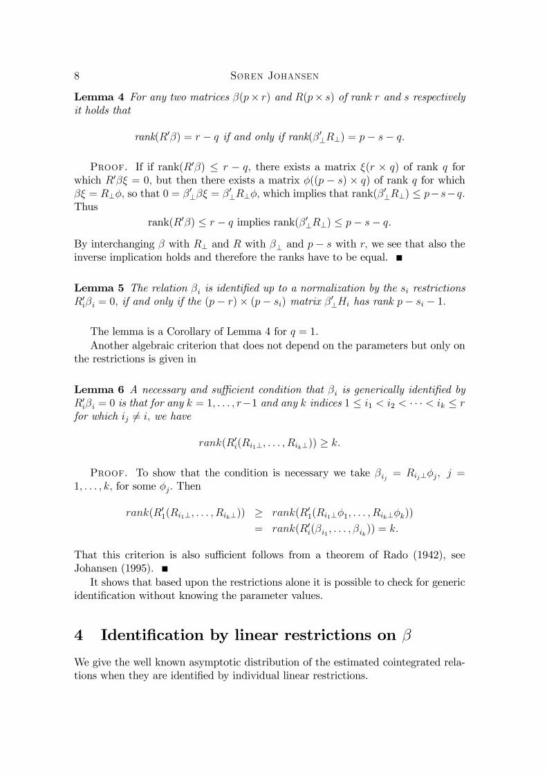
Lemma 4 For any two matrices �(p� r) and R(p� s) of rank r and s respectivelyit holds that

rank(R0�) = r � q if and only if rank(�0?R?) = p� s� q:

Proof. If if rank(R0�) � r � q; there exists a matrix �(r � q) of rank q forwhich R0�� = 0; but then there exists a matrix �((p � s) � q) of rank q for which�� = R?�; so that 0 = �0?�� = �0?R?�; which implies that rank(�

0?R?) � p�s�q:

Thusrank(R0�) � r � q implies rank(�0?R?) � p� s� q:

By interchanging � with R? and R with �? and p� s with r; we see that also theinverse implication holds and therefore the ranks have to be equal.

Lemma 5 The relation �i is identi�ed up to a normalization by the si restrictionsR0i�i = 0; if and only if the (p� r)� (p� si) matrix �

0?Hi has rank p� si � 1:

The lemma is a Corollary of Lemma 4 for q = 1.Another algebraic criterion that does not depend on the parameters but only on

the restrictions is given in

Lemma 6 A necessary and su¢ cient condition that �i is generically identi�ed byR0i�i = 0 is that for any k = 1; : : : ; r�1 and any k indices 1 � i1 < i2 < � � � < ik � rfor which ij 6= i; we have

rank(R0i(Ri1?; : : : ; Rik?)) � k:

Proof. To show that the condition is necessary we take �ij = Rij?�j; j =1; : : : ; k; for some �j: Then

rank(R01(Ri1?; : : : ; Rik?)) � rank(R01(Ri1?�1; : : : ; Rik?�k))

= rank(R0i(�i1 ; : : : ; �ik)) = k:

That this criterion is also su¢ cient follows from a theorem of Rado (1942), seeJohansen (1995).It shows that based upon the restrictions alone it is possible to check for generic

identi�cation without knowing the parameter values.

4 Identi�cation by linear restrictions on �

We give the well known asymptotic distribution of the estimated cointegrated rela-tions when they are identi�ed by individual linear restrictions.


4.1 Asymptotic distribution of � and � with identifying re-strictions on �

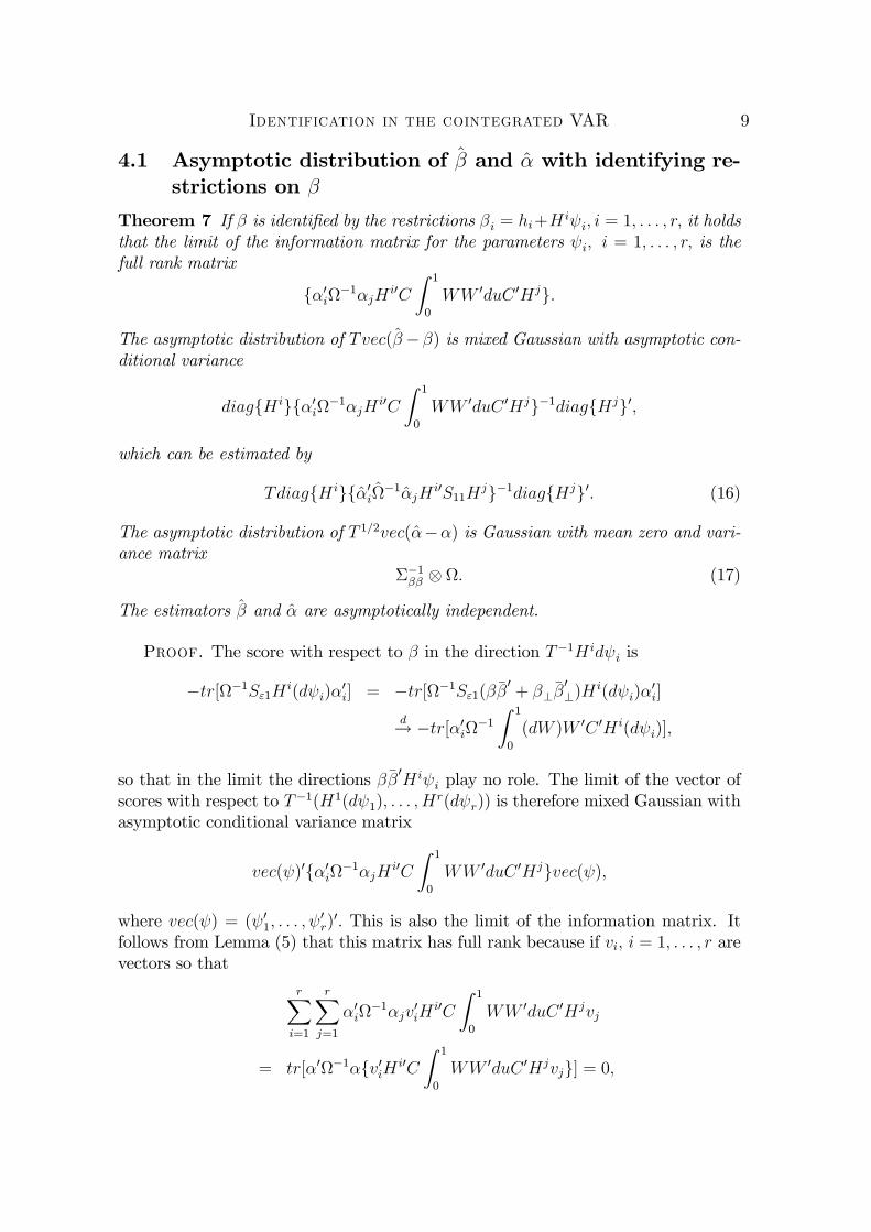
Theorem 7 If � is identi�ed by the restrictions �i = hi+Hi i; i = 1; : : : ; r; it holds

that the limit of the information matrix for the parameters i; i = 1; : : : ; r; is thefull rank matrix

f�0i�1�jH i0C

Z 1

0

WW 0duC 0Hjg:

The asymptotic distribution of Tvec(��) is mixed Gaussian with asymptotic con-ditional variance

diagfH igf�0i�1�jH i0C

Z 1

0

WW 0duC 0Hjg�1diagfHjg0;

which can be estimated by

TdiagfH igf�0i�1�jH i0S11Hjg�1diagfHjg0: (16)

The asymptotic distribution of T 1=2vec(��) is Gaussian with mean zero and vari-ance matrix

��1�� : (17)

The estimators � and � are asymptotically independent.

Proof. The score with respect to � in the direction T�1H id i is

�tr[�1S"1H i(d i)�0i] = �tr[�1S"1(��

0+ �?

��0?)H

i(d i)�0i]

d! �tr[�0i�1Z 1

0

(dW )W 0C 0H i(d i)];

so that in the limit the directions ��0H i i play no role. The limit of the vector ofscores with respect to T�1(H1(d 1); : : : ; H

r(d r)) is therefore mixed Gaussian withasymptotic conditional variance matrix

vec( )0f�0i�1�jH i0C

Z 1

0

WW 0duC 0Hjgvec( );

where vec( ) = ( 01; : : : ; 0r)0: This is also the limit of the information matrix. It

follows from Lemma (5) that this matrix has full rank because if vi; i = 1; : : : ; r arevectors so that

rXi=1

rXj=1

�0i�1�jv

0iH

i0C

Z 1

0

WW 0duC 0Hjvj

= tr[�0�1�fv0iH i0C

Z 1

0

WW 0duC 0Hjvjg] = 0;

10 Søren Johansen

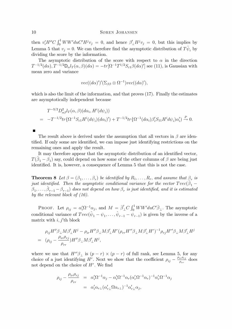
then v0iHi0CR 10WW 0duC 0Hjvj = 0; and hence �0?H

jvj = 0; but this implies byLemma 5 that vj = 0: We can therefore �nd the asymptotic distribution of T i bydividing the score by the information.The asymptotic distribution of the score with respect to � in the direction

T�1=2(d�); T�1=2D�lT (�; �)(d�) = �tr[�1T 1=2S"1�(d�)0] see (11), is Gaussian withmean zero and variance

vec((d�)0)0(�� 1)vec((d�)0);

which is also the limit of the information, and that proves (17). Finally the estimatesare asymptotically independent because

T�3=2D2��lT (�; �)(d�i; H

i(d i))

= �T�1=2trf�1S"1H i(d i)(d�i)0) + T�1=2trf�1(d�i)�0iS11H id i)�

0i)

P! 0:

The result above is derived under the assumption that all vectors in � are iden-ti�ed. If only some are identi�ed, we can impose just identifying restrictions on theremaining ones and apply the result.It may therefore appear that the asymptotic distribution of an identi�ed vector,

T (�1� �1) say, could depend on how some of the other columns of � are being justidenti�ed. It is, however, a consequence of Lemma 5 that this is not the case.

Theorem 8 Let � = (�1; : : : ; �r) be identi�ed by R1; : : : ; Rr; and assume that �r isjust identi�ed. Then the asymptotic conditional variance for the vector Tvec(�1 ��1; : : : ; �r�1��r�1) does not depend on how �r is just identi�ed, and it is estimatedby the relevant block of (16).

Proof. Let �ij = �0i�1�j, and M = ��

0?C

R 10WW 0duC 0��?: The asymptotic

conditional variance of Tvec( 1 � 1; : : : ; r�1 � r�1) is given by the inverse of amatrix with i; j0th block

�ijHi0�?M�0?H

j � �irHi0�?M�0?H

r(�rrHr0�?M�0?H

r)�1�rjHr0�?M�0?H

j

= (�ij ��ir�rj�rr

)H i0�?M�0?Hj;

where we use that Hr0�? is (p � r) � (p � r) of full rank, see Lemma 5, for anychoice of a just identifying Hr: Next we show that the coe¢ cient �ij �

�ir�rj�rr

doesnot depend on the choice of Hr: We �nd

�ij ��ir�rj�rr

= �0i�1�j � �0i

�1�r(�0r

�1�r)�1�0r

�1�j

= �0i�r?(�0r?�r?)

�1�0r?�j;


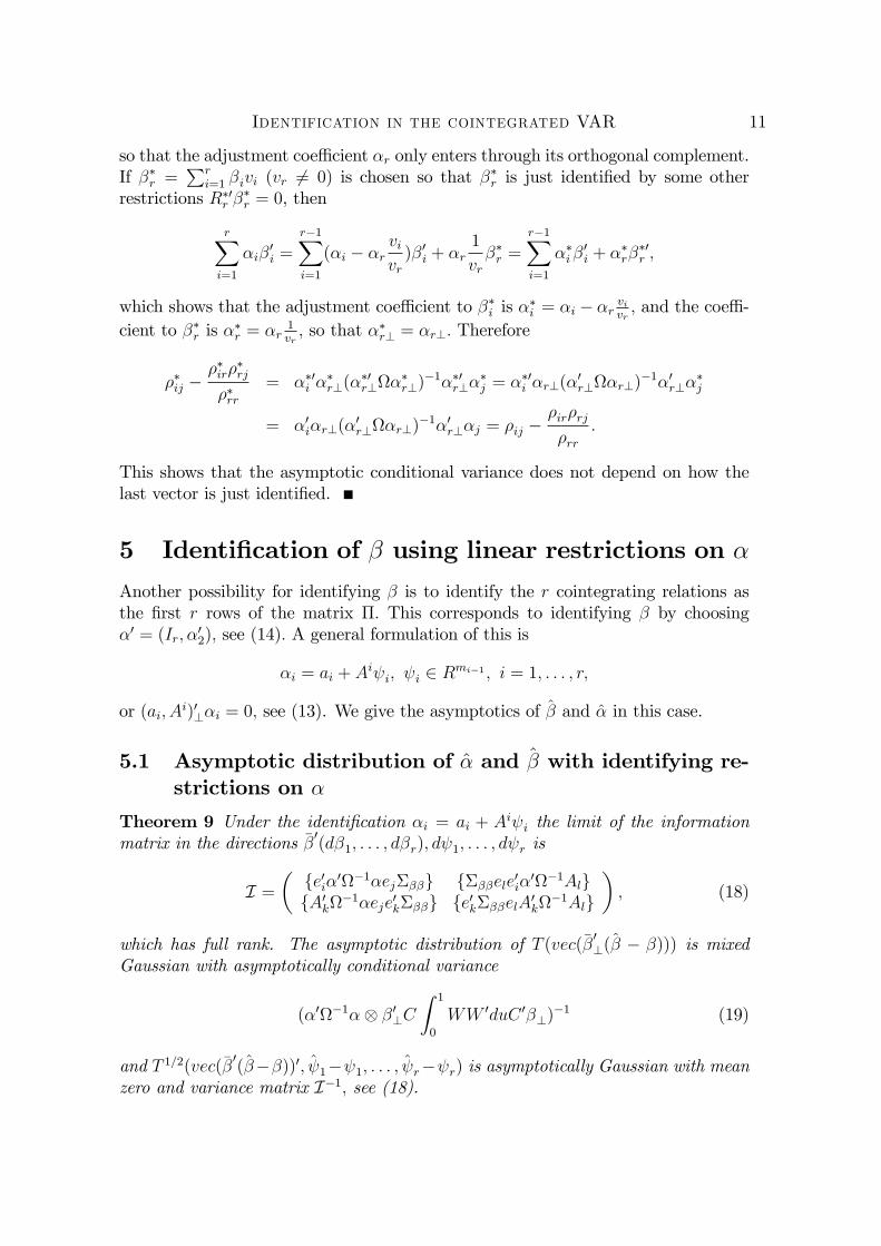
so that the adjustment coe¢ cient �r only enters through its orthogonal complement.If ��r =

Pri=1 �ivi (vr 6= 0) is chosen so that ��r is just identi�ed by some other

restrictions R�0r ��r = 0, then

rXi=1

�i�0i =

r�1Xi=1

(�i � �rvivr)�0i + �r

1

vr��r =

r�1Xi=1

��i�0i + ��r�

�0r ;

which shows that the adjustment coe¢ cient to ��i is ��i = �i � �r vivr ; and the coe¢ -

cient to ��r is ��r = �r

1vr; so that ��r? = �r?: Therefore

��ij ��ir�

�rj

��rr= ��0i �

�r?(�

�0r?�

�r?)

�1��0r?��j = ��0i �r?(�

0r?�r?)

�1�0r?��j

= �0i�r?(�0r?�r?)

�1�0r?�j = �ij ��ir�rj�rr

:

This shows that the asymptotic conditional variance does not depend on how thelast vector is just identi�ed.

5 Identi�cation of � using linear restrictions on �

Another possibility for identifying � is to identify the r cointegrating relations asthe �rst r rows of the matrix �: This corresponds to identifying � by choosing�0 = (Ir; �

02); see (14): A general formulation of this is

�i = ai + Ai i; i 2 Rmi�1 ; i = 1; : : : ; r;

or (ai; Ai)0?�i = 0; see (13). We give the asymptotics of � and � in this case.

5.1 Asymptotic distribution of � and � with identifying re-strictions on �

Theorem 9 Under the identi�cation �i = ai + Ai i the limit of the informationmatrix in the directions ��0(d�1; : : : ; d�r); d 1; : : : ; d r is

I =�fe0i�0�1�ej��g f��ele0i�0�1AlgfA0k�1�eje0k��g fe0k��elA0k�1Alg

�; (18)

which has full rank. The asymptotic distribution of T (vec(��0?(� � �))) is mixedGaussian with asymptotically conditional variance

(�0�1� �0?C

Z 1

0

WW 0duC 0�?)�1 (19)

and T 1=2(vec(��0(��))0; 1� 1; : : : ; r� r) is asymptotically Gaussian with meanzero and variance matrix I�1; see (18).

12 Søren Johansen

In the special case where Ai = A; i = 1; : : : ; r; the covariance matrix I�1 becomes�fe0i(�0A?(A0?A?)�1A0?�)�1ej��1��g �f��1��ele0i(�0�1�)�1�0�1AMg�fMA0�1�(�0�1�)�1eje

0k�

�1��g fe0k��1��elMg

�; (20)

where M = (A0�?(�0?�?)

�1�0?A)�1: When we identify � by � = (Ir; �02)

0 we haveA = (0; Ip�r); and �nd the asymptotic variance matrix for T 1=2(vec(��

0(� � �)))

��1�� 1:r;1:r:

Proof. Proof see the appendixThe results of Theorem 9 show that the asymptotic distribution of � has two

components: one in the direction of � which is T 1=2 consistent and one in thedirection of �? which is T consistent. It follows that

T 1=2(� � �) = T 1=2��0(� � �) + T 1=2�?

��0?(� � �) = T 1=2��

0(� � �) + oP (1):

Thus, the distribution of T 1=2(��) is asymptotically Gaussian, but with a singularcovariance matrix, so there are some hypotheses that one cannot test using theGaussian distribution. We illustrate by an example.

Example 3 Suppose we have four variables and two cointegrating relations, andwe identify using �0 = (I2; �

02) so that the �rst two rows of � are the identi�ed

cointegrating parameters. Now assume that the true value � has �11 = 0. We cantest this hypothesis by applying the asymptotic Gaussian distribution of �11 :

T 1=2�11qe01e1e

01��

�1��0e1

d! N(0; 1); (21)

where

e01��1��

0e1 = (�11; �12)��1�� (�11; �12)

0 = (0; �12)��1�� (0; �12)

0 = (�12)2(��1�� )22:

Thus we see that (21) only holds if �12 6= 0: In this case we let BT = (�; T�1=2�?)and �nd a consistent estimator of e01��

�1�0e1 from

e01S�111 e1 = e01BT (B

0TS11BT )

�1B0T e1 (22)

= e01��1��

0e1 + T�1e01�?(T�1�0?S11�?)

�1�0?e1 + oP (1)P! e01��

�1��

0e1:

Thus a simulation experiment will show that �11 is approximately Gaussian incase �12 6= 0: If, however, �12 = 0; that is, � has the �rst row equal to zero, �0e1 = 0;we cannot use the asymptotic result (21), and �nd instead that

T �11 = Te01(� � �)e1 = Te01��0(� � �)e1 + Te01�?

��0?(� � �)e1 = Te01�?

��0?(� � �)e1

d! e01�?(�0?C

Z 1

0

WW 0duC 0�?)�1�0?C

Z 1

0

W (dW )0�1�1;


and because e01� = 0; we have e01�? 6= 0. Thus in case �12 = 0; the simulation above

will show that �11 is not approximately Gaussian, but mixed Gaussian, which meansthat we no longer want to normalize by the standard error, but by an estimate ofthe asymptotic conditional standard error. Thus in this case inference is not basedon the asymptotic distribution of �11 but on the joint asymptotic distribution of �11and the observed information e01e1e

01S

�111 e1.

Thus, the mixed Gaussian limit has to be used to make inference on �11: Note,however, that one can use the same statistic:

T 1=2�11qe01e1e

01S

�111 e1

=T �11q

e01e1e01(T

�1S11)e1

d! N(0; 1);

because in this case, it follows from (22) that when e01� = 0;

e01(T�1S11)

�1e1 = e01�?(T�1�0?S11�?)

�1�0?e1 + oP (1)

d! e01�?(�0?C

Z 1

0

WW 0duC 0�?)�1�0?e1;

so that T �11 is normalized by an estimator of the square root of its asymptoticconditional variance, which is the appropriate scaling factor, and the limit is againN(0; 1).The di¤erence between the situation �21 = 0 and �21 6= 0; is that if �21 6= 0; the

hypothesis �11 = 0 does not change the cointegration space. When �21 6= 0; it ispossible to change the coordinate system inside sp(�) and obtain �11 = 0; that is�nd a linear combination of �1 and �2 with �rst coe¢ cient zero: If �21 = 0; however,this is not possible in general and the hypothesis �11 = 0; becomes a hypothesis onthe cointegrating space leading to mixed Gaussian inference.�

5.1.1 Discussion.

The mathematical formulation of all this is that it is the cointegration space whichis estimated superconsistently and the estimator is mixed Gaussian and asymptoti-cally independent of the limit of the remaining parameters. The problem is how toreformulate this statement into something that is economically useful. This is whatis done by the identifying restrictions of the form R0i�i = 0; whereby the cointegrat-ing space is parameterized using economically meaningful parameters. On the otherhand, identifying the cointegration space as the �rst two rows, say, of the matrix �;that is, as the stationary linear combination to which the �rst two variables react, isclearly an identi�cation of the cointegration space, but it also speci�es which vectorsin that space we are interested in. Thus if the �rst two rows of � are

�0 =

��11 �21 �31 �41�12 �22 �32 �42

�;

it is clear that by multiplying by the matrix��22 ��21��12 �11

�;

14 Søren Johansen

we get ��11�22 � �12�21 0 � �

0 �11�22 � �12�21 � �

�:

This does not change the cointegrating space, but we can achieve zeros at the po-sitions 12 and 21: Thus the hypothesis that, say, �12 = �21 = 0; is clearly testable,because the parameters are identi�ed, but it is not a hypothesis on the cointegrationspace and hence does not involve mixed Gaussian inference.

6 Shocks and their e¤ect

The cointegrated vector autoregressive model associates with each variable Xit acontemporaneous shock "it; which is the unanticipated part of Xit given the past.The identi�cation of shocks is often done by postulating an ordering of the variables,and therefore the corresponding shocks, and perform a Cholesky decomposition ofthe variance : If we decompose the shock into a permanent �0?"t and a transitorypart, �0�1"t, there is no natural ordering because of the lack of identi�cation of(�; �?): We propose to give names to the permanents shocks by considering theire¤ects on the process, that is, by analyzing the long-run variance

CC 0;

see (3). Similarly we give names to the transitory shocks by considering their e¤ecton the equations given the long-run shocks. This leads to an analysis of the short-runvariance

BB0 = �(�0�1�)�1�0:

If we apply a Cholesky decomposition of CC 0 or BB0 we �nd linear combinationsof shocks. We end this section by �nding the asymptotic variances of these estimatedlinear combinations.

6.1 Permanent and transitory shocks and their contempo-raneous and permanent e¤ects

Model (1) can be written as

Xt = (Ip + ��0)Xt�1 +

kXi=1

�i�Xt�i + "t:

This shows that a change in "t ("t 7! "t + c) is equivalent to a change in Xt (Xt 7!Xt + c): We now discuss the e¤ect of such a change on later values Xt+h; using theGranger representation theorem (2). We �nd

Xt+h = C

t+hXi=1

"i +

1Xi=0

Ci"t+h�i + A;


which shows that the e¤ect at time t+ h of a change c 2 Rp to "t (or Xt) is

@Xt+h

@"tc = (C + Ch)c! Cc; h!1:

A change c to the system at time t propagates through the system and becomes Ccin the long run, that is, the permanent e¤ect of a change is Cc: Moreover from theexpression for C; see (3), we see that the part of the shock "t; which has an e¤ectin the long run is �0?"t:We note the decomposition of "t into independent components

"t = �(�0�1�)�1�0�1"t + �?(�0?�?)

�1�0?"t: (23)

Based on this we use the de�nitions

De�nition 10 We call "t the shock at time t; and de�ne the permanent shock as�0?"t and the transitory shock as �

0�1"t: We de�ne the contemporaneous e¤ect of"t as Ip:From the decomposition (23) of the shock "t; we �nd the contemporaneous e¤ect

of the permanent shock, �0?"t; is �?(�0?�?)

�1; and that of a transitory shock,�0�1"t; is �(�0�1�)�1:Finally the long-run e¤ect of a shock "t is de�ned to be C; of a permanent shock it

is C�?(�0?�?)�1 = �?(�

0?��?)

�1; and of a transitory shock it is C�(�0�1�)�1 =0.

7 Identi�cation of permanent shocks

We start by an example.Example 4 Let us assume we have among others the real variable yrt and the

nominal variable pt; and that we have two permanent shocks, which we want to calla real shock and a nominal shock. The Granger representation of the variables is

yrt = e01C

tXi=1

"i + z1t = c01

tXi=1

"i + z1t;

pt = e02C

tXi=1

"i + z2t = c02

tXi=1

"i + z2t;

...

It seems clear that we want the permanent shocks to be de�ned by �0?"t: The problemis to identify which shock can in�uence which variable.Let us assume that

A nominal shock cannot have a permanent in uence on a real variable

16 Søren Johansen

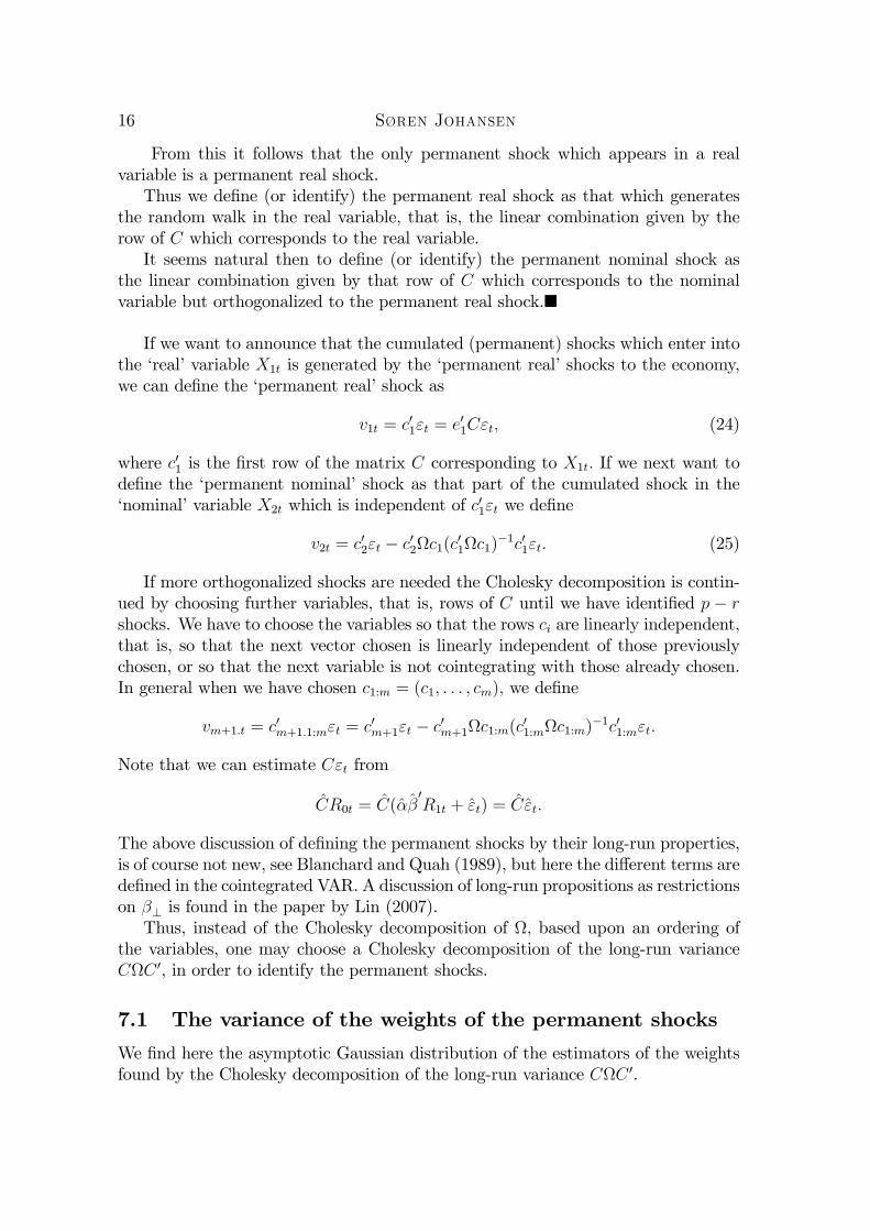
From this it follows that the only permanent shock which appears in a realvariable is a permanent real shock.Thus we de�ne (or identify) the permanent real shock as that which generates

the random walk in the real variable, that is, the linear combination given by therow of C which corresponds to the real variable.It seems natural then to de�ne (or identify) the permanent nominal shock as

the linear combination given by that row of C which corresponds to the nominalvariable but orthogonalized to the permanent real shock.�

If we want to announce that the cumulated (permanent) shocks which enter intothe �real�variable X1t is generated by the �permanent real�shocks to the economy,we can de�ne the �permanent real�shock as

v1t = c01"t = e01C"t; (24)

where c01 is the �rst row of the matrix C corresponding to X1t: If we next want tode�ne the �permanent nominal�shock as that part of the cumulated shock in the�nominal�variable X2t which is independent of c01"t we de�ne

v2t = c02"t � c02c1(c01c1)

�1c01"t: (25)

If more orthogonalized shocks are needed the Cholesky decomposition is contin-ued by choosing further variables, that is, rows of C until we have identi�ed p � rshocks. We have to choose the variables so that the rows ci are linearly independent,that is, so that the next vector chosen is linearly independent of those previouslychosen, or so that the next variable is not cointegrating with those already chosen.In general when we have chosen c1:m = (c1; : : : ; cm); we de�ne

vm+1:t = c0m+1:1:m"t = c0m+1"t � c0m+1c1:m(c01:mc1:m)

�1c01:m"t:

Note that we can estimate C"t from

CR0t = C(��0R1t + "t) = C"t:

The above discussion of de�ning the permanent shocks by their long-run properties,is of course not new, see Blanchard and Quah (1989), but here the di¤erent terms arede�ned in the cointegrated VAR. A discussion of long-run propositions as restrictionson �? is found in the paper by Lin (2007).Thus, instead of the Cholesky decomposition of ; based upon an ordering of

the variables, one may choose a Cholesky decomposition of the long-run varianceCC 0, in order to identify the permanent shocks.

7.1 The variance of the weights of the permanent shocks

We �nd here the asymptotic Gaussian distribution of the estimators of the weightsfound by the Cholesky decomposition of the long-run variance CC 0.


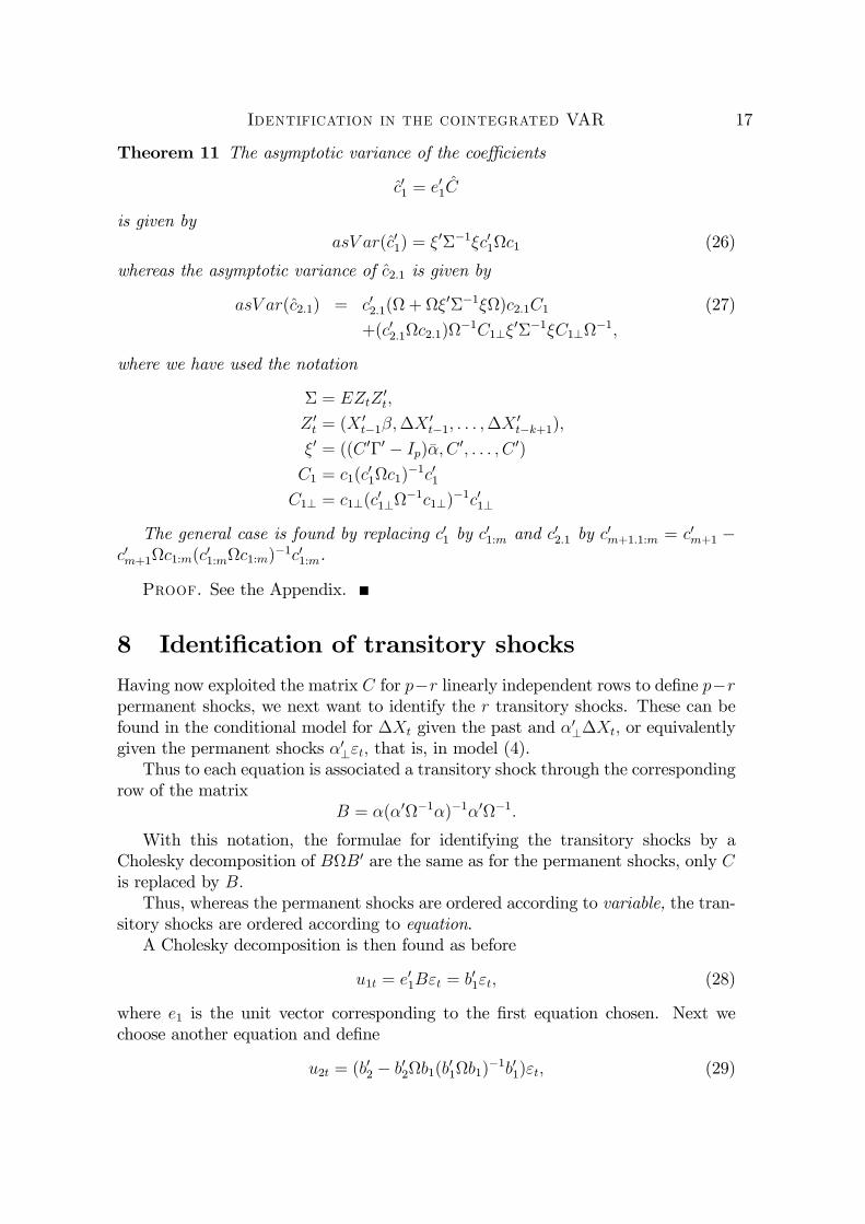
Theorem 11 The asymptotic variance of the coe¢ cients

c01 = e01C

is given byasV ar(c01) = �0��1�c01c1 (26)

whereas the asymptotic variance of c2:1 is given by

asV ar(c2:1) = c02:1( + �0��1�)c2:1C1 (27)

+(c02:1c2:1)�1C1?�

0��1�C1?�1;

where we have used the notation

� = EZtZ0t;

Z 0t = (X0t�1�;�X

0t�1; : : : ;�X

0t�k+1);

�0 = ((C 0�0 � Ip)��;C0; : : : ; C 0)

C1 = c1(c01c1)

�1c01C1? = c1?(c

01?

�1c1?)�1c01?

The general case is found by replacing c01 by c01:m and c

02:1 by c

0m+1:1:m = c0m+1 �

c0m+1c1:m(c01:mc1:m)

�1c01:m.

Proof. See the Appendix.

8 Identi�cation of transitory shocks

Having now exploited the matrix C for p�r linearly independent rows to de�ne p�rpermanent shocks, we next want to identify the r transitory shocks. These can befound in the conditional model for �Xt given the past and �0?�Xt; or equivalentlygiven the permanent shocks �0?"t; that is, in model (4).Thus to each equation is associated a transitory shock through the corresponding

row of the matrixB = �(�0�1�)�1�0�1:

With this notation, the formulae for identifying the transitory shocks by aCholesky decomposition of BB0 are the same as for the permanent shocks, only Cis replaced by B:Thus, whereas the permanent shocks are ordered according to variable, the tran-

sitory shocks are ordered according to equation.A Cholesky decomposition is then found as before

u1t = e01B"t = b01"t; (28)

where e1 is the unit vector corresponding to the �rst equation chosen. Next wechoose another equation and de�ne

u2t = (b02 � b02b1(b

01b1)

�1b01)"t; (29)

18 Søren Johansen

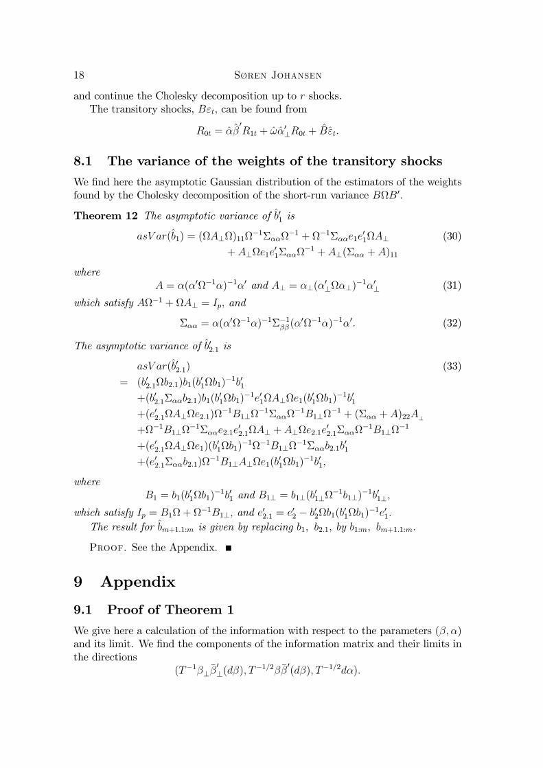
and continue the Cholesky decomposition up to r shocks.The transitory shocks, B"t; can be found from

R0t = ��0R1t + !�0?R0t + B"t:

8.1 The variance of the weights of the transitory shocks

We �nd here the asymptotic Gaussian distribution of the estimators of the weightsfound by the Cholesky decomposition of the short-run variance BB0.

Theorem 12 The asymptotic variance of b01 is

asV ar(b1) = (A?)11�1��

�1 + �1��e1e01A? (30)

+ A?e1e01��

�1 + A?(�� + A)11

whereA = �(�0�1�)�1�0 and A? = �?(�

0?�?)

�1�0? (31)

which satisfy A�1 + A? = Ip; and

�� = �(�0�1�)�1��1�� (�0�1�)�1�0: (32)

The asymptotic variance of b02:1 is

asV ar(b02:1) (33)

= (b02:1b2:1)b1(b01b1)

�1b01+(b02:1��b2:1)b1(b

01b1)

�1e01A?e1(b01b1)

�1b01+(e02:1A?e2:1)

�1B1?�1��

�1B1?�1 + (�� + A)22A?

+�1B1?�1��e2:1e

02:1A? + A?e2:1e

02:1��

�1B1?�1

+(e02:1A?e1)(b01b1)

�1�1B1?�1��b2:1b

01

+(e02:1��b2:1)�1B1?A?e1(b

01b1)

�1b01;

whereB1 = b1(b

01b1)

�1b01 and B1? = b1?(b01?

�1b1?)�1b01?;

which satisfy Ip = B1 + �1B1?; and e02:1 = e02 � b02b1(b

01b1)

�1e01:

The result for bm+1:1:m is given by replacing b1; b2:1; by b1:m; bm+1:1:m:

Proof. See the Appendix.

9 Appendix

9.1 Proof of Theorem 1

We give here a calculation of the information with respect to the parameters (�; �)and its limit. We �nd the components of the information matrix and their limits inthe directions

(T�1�?��0?(d�); T

�1=2��0(d�); T�1=2d�):


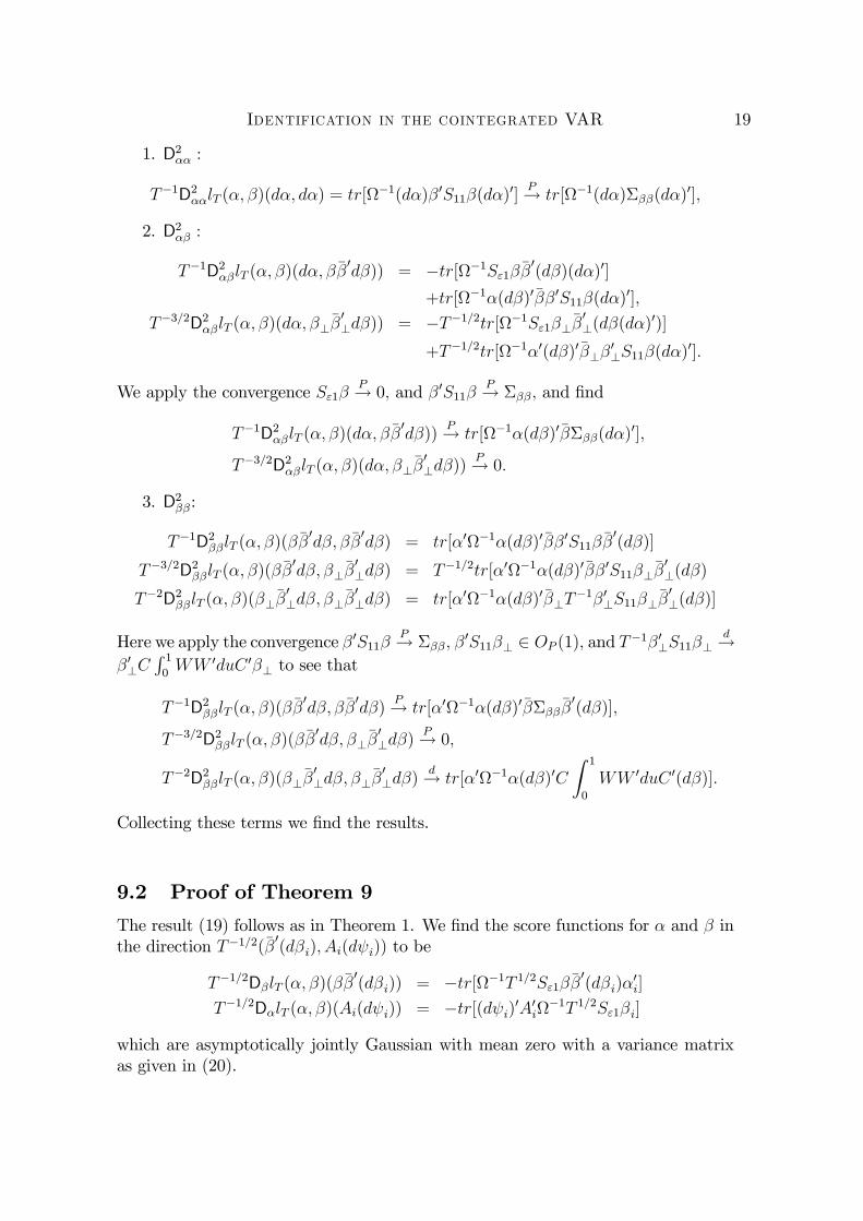
1. D2�� :

T�1D2��lT (�; �)(d�; d�) = tr[�1(d�)�0S11�(d�)0]

P! tr[�1(d�)��(d�)0];

2. D2�� :

T�1D2��lT (�; �)(d�; ��0d�)) = �tr[�1S"1��

0(d�)(d�)0]

+tr[�1�(d�)0��0S11�(d�)0];

T�3=2D2��lT (�; �)(d�; �?��0?d�)) = �T�1=2tr[�1S"1�?��

0?(d�(d�)

0)]

+T�1=2tr[�1�0(d�)0��?�0?S11�(d�)

0]:

We apply the convergence S"1�P! 0; and �0S11�

P! ��; and �nd

T�1D2��lT (�; �)(d�; ��0d�))

P! tr[�1�(d�)0��(d�)0];

T�3=2D2��lT (�; �)(d�; �?��0?d�))

P! 0:

3. D2��:

T�1D2��lT (�; �)(��0d�; ��

0d�) = tr[�0�1�(d�)0��0S11��

0(d�)]

T�3=2D2��lT (�; �)(��0d�; �?

��0?d�) = T�1=2tr[�0�1�(d�)0��0S11�?

��0?(d�)

T�2D2��lT (�; �)(�?��0?d�; �?

��0?d�) = tr[�0�1�(d�)0��?T

�1�0?S11�?��0?(d�)]

Here we apply the convergence �0S11�P! ��; �

0S11�? 2 OP (1); and T�1�0?S11�?d!

�0?CR 10WW 0duC 0�? to see that

T�1D2��lT (�; �)(��0d�; ��

0d�)

P! tr[�0�1�(d�)0��0(d�)];

T�3=2D2��lT (�; �)(��0d�; �?

��0?d�)

P! 0;

T�2D2��lT (�; �)(�?��0?d�; �?

��0?d�)

d! tr[�0�1�(d�)0C

Z 1

0

WW 0duC 0(d�)]:

Collecting these terms we �nd the results.


The result (19) follows as in Theorem 1. We �nd the score functions for � and � inthe direction T�1=2(��0(d�i); Ai(d i)) to be

T�1=2D�lT (�; �)(��0(d�i)) = �tr[�1T 1=2S"1��

0(d�i)�

0i]

T�1=2D�lT (�; �)(Ai(d i)) = �tr[(d i)0A0i�1T 1=2S"1�i]

which are asymptotically jointly Gaussian with mean zero with a variance matrixas given in (20).

20 Søren Johansen

In the special case where Ai = A we can invert the information matrix and �nd�fe0i�0�1�ej��g f��ele0i�0�1AgfA0�1�eje0k�g fe0k��elA0�1Ag

��1=

�M11 M12

M21 M22

�:

We �rst �nd that fe0k��elA0�1Ag�1 = fe0k��1��el(A0�1A)�1g; and therefore, for�ij = �0i

�1�j;

(M�111 )ij = �ij��

Xl;k

��ele0i�0�1Ae0k�

�1��el(A

0�1A)�1A0�1�eje0k��

= �ij�� Xl;k

��ele0k�

�1��ele

0k��[e

0i�0�1A(A0�1A)�1A0�1�ej]

NowP

l;k ��ele0l��1��eke

0k�� = ��

�1�� = ��; and hence

(M�111 )ij = e0i[�

0�1�� 0�1A(A0�1A)�1A0�1�]ej��

= e0i[�0A?(A

0?A?)

�1A?�]ej��

and thereforeM11 = fe0i(�0A?(A0?A?)�1A?�)�1ej��1��g:

Similarly we �nd

(M�122 )kl = �klA

0�1A�Xi;j

(A0�1�eje0k��e

0i(�

0�1�)�1ej��1��ele

0i�0�1A

= �klA0�1A� e0k��el

Xi;j

(A0�1�eje0i(�

0�1�)�1eje0i�0�1A

= �kl[A0�1A� (A0�1�(�0�1�)�1�0�1A]

= �kl[A0�?(�

0?�?)

�1�0?A]:

HenceM22 = fe0l��1��ek[A0�?(�0?�?)�1�0?A]�1g:

The o¤-diagonal elements are found from

f�ij��gM12 + f��ele0i�0�1AgM22 = 0;

which implies that

(M12)il = �Xk;m

�ik��1��eme0k�

0�1A�mlM

= �Xm

eme0m�

�1��el

Xk

e0i(�0�1�)�1eke

0k�

0�1AM

= ��1��ele0i(�0�1�)�1�0�1AM:

In particular for A = (0; Ip�r)0 we �nd, using �0A? = Ir; and A? = (Ir; 0)0

M11 = fe0i(�0A?(A0?A?)�1A?�)�1ej��1��g= fe0i�1ej��1g = 11 ��1�� :



We want to derive the asymptotic distribution in Theorem 11 using the ��method.For this we need the asymptotic distribution of (C; ); which is asymptoticallyGaussian with variance matrix given by the next lemma and an expansion of c2:1 asfunction of C and .

Lemma 13 The asymptotic variance and covariance matrix of and C are givenby

asV ar(�0�) = (�0�)(�0�) + (�0�)2;

asV ar(�0C�) = (�0�0��1��)(�0CC 0�);

asCov(; C) = 0;

where

� = EZtZ0t;

Z 0t = (X0t�1�;�X

0t�1; : : : ;�X

0t�k+1);

�0 = ((C 0�0 � Ip)��;C0; : : : ; C 0):

see Paruolo (1997). We also need the derivatives of

c02:1 = c02 � c02c1(c01c1)

�1c01 = [e02 � e02CC

0e1(e01CC

0e1)�1e01]C

with respect to C and :

Lemma 14 We have the expansion

d(c02 � c02c1(c01c1)

�1c01)

= (e02 � c02c1(c01c1)

�1e01)(dC)C1?�1 � c02:1(d)C1 � c02:1(dC)

0e1(c01c1)

�1c01;

where C1 = c1(c01c1)

�1c01 and C1? = c1?(c01?

�1c1?)�1c01?:

Proof. By Taylor�s expansion we �nd

d(c02 � c02c1(c01c1)

�1c01)

= (dc2)0 � (dc2)0c1(c01c1)�1c01 � c02(d)c1(c

01c1)

�1c01 � c02(dc1)(c01c1)

�1c01+ c02c1(c

01c1)

�1((dc1)0c1 + c01(d)c1 + c01(dc1))(c

01c1)

�1c01 � c02c1(c01c1)

�1(dc1)0

= e02(dC)(Ip � C1)� c02:1(d)C1 � c02[Ip � C1]

(dC)0e1(c01c1)

�1c01 � c02c1(c01c1)

�1(dC)0e1C1?�1

= e02(dC)C1?�1 � c02:1(d)C1

� c02:1(dC)0e1(c

01c1)

�1c01 � c02c1(c01c1)

�1e01(dC)C1?�1;

which reduces to the result.

22 Søren Johansen

We start the proof of Theorem 11 by (26), which follows directly from the ex-pression for the asymptotic variance of C :

asV ar(c01�) = asV ar(e01C�) = (�0�0��1��)(e01CC

0e1) = (�0�0��1��)(c01c1):

We next prove (27). We �nd from Lemma 14 that, for e02:1 = e02� c02c1(c01c1)�1e01;it holds that

(dc2:1)0� = �c02:1(d)C1� + e02:1(dC)C1?

�1� � �0c1(c01c1)

�1e01(dC)c2:1;

so that

asV ar(c02:1�) = asV ar(�c02:1C1� + e02:1CC1?�1� � �0c1(c

01c1)

�1e01Cc2:1)

= asV ar(K +K1 +K2):

We �rst �nd the variances

asV ar(K) = (c02:1c2:1)(�

0C1C1�) + (c02:1C1�)

2 = (c02:1c2:1)(�0C1�)

because C1C1 = C1 and c02:1C1 = 0: Next

asV ar(K1) = (�0�1C1?�

0��1�C1?�1�)(c02:1c2:1):

Finally

asV ar(K2) = (c02:1�

0��1�c2:1)(�0c1(c

01c1)

�1e01CC0e1(c

01c1)

�1c01�)

= (c02:1�0��1�c2:1)(�

0C1�):

We have Cov(K;K1) = Cov(K;K2) = 0; because C and are asymptoticallyindependent, see Lemma 13, and �nd

asCov(K1;K2) = �asCov[e02:1CC1?�1�; �0c1(c01c1)�1e01Cc2:1]= (e02:1CC

0e1(c01c1)

�1c01�)(c02:1�

0��1�C1?�1�)

= (c02:1C1�)(c02:1�

0��1�C1?�1�) = 0;

because c02:1C1 = 0: Collecting the result, we have proved (27). The general case isproved the same way by replacing c1 by c1:m. This completes the proof of Theorem11.


We �rst �nd an expansion of B as a function of and �; and apply this to �nd theasymptotic distribution of (B; ):

Lemma 15 We have the expansions

dB = d(�(�0�1�)�1�0�1) (34)

= A?(d�)(�0�1�)�1�0�1 + �(�0�1�)�1(d�)0A? � A�1(d)A?;

where A = �(�0�1�)�1�0 and A? = �?(�0?�?)

�1�0?:


Proof. By Taylor�s expansion we �nd

d�1 = ��1(d)�1

and

d(�0�1�)�1 = �(�0�1�)�1[(d�)0�1��0�1(d)�1�+�0�1(d�)](�0�1�)�1

so that

d(�(�0�1�)�1�0�1)

= (d�)(�0�1�)�1�0�1 + �(�0�1�)�1(d�)0�1 � �(�0�1�)�1�0�1(d)�1

� �(�0�1�)�1[(d�)0�1�� 0�1(d)�1�+ �0�1(d�)](�0�1�)�1�0�1

This expression is the same as in (34), as can be seen by multiplying both by thematrix (�?; �).The asymptotic variance of �; see Johansen (1996), is given by

asCov(�0��; �0��) = (�0�)(�0��1��)

�� = V ar(�0Xtj�Xt; : : : ;�Xt�k+1);

asCov(�; ) = 0;

and we apply that to �nd the asymptotic variance of (B; ):

Lemma 16 The asymptotic variance of B = �(�0�1�)�1�0�1 is

asCov(�0B�; �0B�) (35)

= (�0A?�)(�0�1��

�1�) + (�0�1��)(�0A?�)

+ (�0A?�)(�0��

�1�) + (�0A?�)(�0[�� + A]�);

and the covariance with is

asCov(�0B�; �0�) = �(�0A�)(�0A?�); (36)

where A and A? are given in Lemma 15, and

�� = �(�0�1�)�1��1�� (�0�1�)�1�0:

Proof. We �nd from the expansion of B in Lemma 15 that (� = �(��1�)�1)

asCov(�0B�; �0B�)

= asCov(�0A?��0

�1� + �0��0A?� � �0A�1A?�;

�0A?��0

�1�+ �0��0A?�� 0A�1A?�);

24 Søren Johansen

We �rst take the terms with :

asCov(�0A�1A?�; �0A�1A?�)

= (�0A�1�1A�)(�0A?A?�) + (�0A�1A?�)(�

0A�1A?�)

= (�0A�)(�0A?�);

becauseA�1A? = 0; A�1A = A; A?A? = A?:

Next consider the terms involving � and �0

asCov(�0A?��0

�1� + �0��0A?�; �

0A?��0

�1�+ �0��0A?�)


�1� + �0A?��0�; �

0A?��0

�1�+ �0A?��0�)

= (�0A?�)(�0�1�0�

�1��

0

�1�) + (�0A?�)(�0�1��

�1��

0�)

+ (�0A?�)(�0��

�1��

0

�1�) + (�0A?�)(�0��

�1��

0�):

Introducing �� = ��1��

0 we have proved (35), because � and are asymptoti-

cally independent.Next consider (36), where we again use the asymptotic independence of � and

to �nd

asCov(�0B�; �0�)


�1� + �0��0A?� � �0A�1A?�; �

0�)

= �asCov(�0A�1A?�; �0�) = �(�0A�1�)(�0A?�):

We start the proof of Theorem 12 by (30). We apply (35) of Lemma 16 with� = � = e1; and � = � = to �nd the asymptotic variance of b1 :

asCov(e01B ; e01B )

= (A?)11 0�1��

�1 + 0�1��e1e01A?

+ 0A?e1e01��

�1 + (�� + A)11 0A? ;

which shows (30).Next we prove (33). We apply Lemma 14 with C replaced by B to �nd the

expansion

(db2:1)0 = �b02:1(d)B1 +(e02�b02b1(b01b1)�1e01)(dB)B1?�1 � 0b1(b01b1)�1e01(dB)b2:1;

so that

asV ar(b02:1 ) = asV ar(�b02:1B1 + (e02 � b02b1(b

01b1)

�1e01)BB1?�1 � 0b1(b

01b1)

�1e01Bb2:1)

= asV ar(L + L1 + L2)


9.4.1 The variances

We �rst �nd the variances:

asV ar(L) = asV ar(�b02:1B1 ) = (b02:1b21)( 0B1B1 ) + (b02:1B1 )2

= (b02:1b21)( 0B1 );

because B1B1 = B1 and b02:1B1 = 0:Next we consider asV ar(L1) = asV ar((e02�b02b1(b01b1)�1e01)BB1?�1 ) which

follows from (35) for � = � = e02 � b02b1(b01b1)

�1e01 = e02:1; say, and � = � =B1?

�1

asV ar(L1)

= ( 0�1B1?�1��

�1B1?�1 )(e02:1A?e2:1) + (e

02:1��e2:1)(

0A? )

+ 2( 0�1B1?�1��e2:1)(e

02:1A? ) + (e

02:1Ae2:1)(

0A? );

using A?B1? = A?.Similarly we �nd asV ar(L2) = asV ar( 0b1(b

01b1)

�1e01Bb2:1) from (35) for � =� = e1(b

01b1)

�1b01 and � = � = b2:1

asV ar(L2)

= (b02:1�1��

�1b2:1)( 0b1(b

01b1)

�1e01A?e1(b01b1)

�1b01 )

+ ( 0b1(b01b1)

�1e01��e1(b01b1)

�1b01 )(b02:1A?b2:1)

+ 2(b02:1�1��e1(b

01b1)

�1b01 )( 0b1(b

01b1)

�1e01A?b2:1)

+ ( 0b1(b01b1)

�1e01Ae1(b01b1)

�1b01 )(b02:1A?b2:1)

= (b02:1��b2:1)( 0b1(b

01b1)

�1e01A?e1(b01b1)

�1b01 );

because A?b2:1 = 0; so that only the �rst term is non-zero:

9.4.2 The covariances

We �rst take the covariance asCov(L1;L) = �asCov(e02:1BB1?�1 ; b02:1B1 )which we calculate from (36) for � = e2:1; � = b2:1; � = B1?

�1 ; and � = B1

asCov(L;L1) = �(e02:1Ab2:1)( 0�1B1?A?B1 ) = 0:

because A?B1 = 0:Next asCov(L2;L) = asCov( 0b1e

01Bb2:1; b

02:1B1 ) can be found for

� = e1(b01b1)

�1b01 ; � = b2:1; � = b2:1; � = B1 ;

which gives

asCov(L;L2) = ( 0(b01b1)

�1b01e01Ab2:1)(b

02:1A?B1 ) = 0;

26 Søren Johansen

because b02:1A? = 0:

asCov(�0B�; �0B�)

= (�0A?�)(�0�1��

�1�) + (�0�1��)(�0A?�)

+ (�0A?�)(�0��

�1�) + (�0A?�)(�0[�� + A]�)

Finally asCov(L1;L2) = Cov(e02:1BB1?�1 ; 0b1(b

01b1)

�1e01Bb2:1) can be foundfrom (35) for �0 = e02:1; �

0 = 0b1(b01b1)

�1e01; � = B1?�1 ; � = b2:1. We note

that A?� = A?b2:1 = 0; so we only need to consider the terms

(�0A?�)(�0�1��

�1�) + (�0A?�)(�0��

�1�)

= ( 0�1B1?�1��b2:1)(e

02:1A?e1)(b

01b1)

�1b01

+ (e02:1��b2:1)( 0�1B1?A?e1(b

01b1)

�1b01 )

Collecting the terms we have proved the result.�

10 References

Blanchard, O. F. and D. Quah 1989. The dynamic e¤ects of aggregate demandand supply disturbances. American Economic Review 79, 655�673.Fisher, F. M. 1966. The Identi�cation Problem in Econometrics. McGraw-Hill.

New York NY.Johansen S., 1995. Identifying Restrictions of Linear Equations � with appli-

cations to simultaneous equations and cointegration. Journal of Econometrics 69,111�132.Johansen, S. 1996. Likelihood-Based Inference in Cointegrated Vector Autore-

gressive Models. Oxford University Press, Oxford (2.ed.).Lin. M.-T. 2007. Long-run propositions, long-run identi�cation, and cointegrat-

ing relations. Discussion paper. National University of Singapore.Paruolo P. 1997. Asymptotic inference on the moving average impact matrix in

cointegrated I(1) VAR systems, Econometric Theory, 13, 79�118.Rado, R. 1942. A theorem on independence relations. Quarterly Journal of

Mathematics, Oxford 13, 83�89.van der Vaart, A. W. 1998. Asymptotic Statistics. Cambridge University Press,

Cambridge.

Documents

Some identi–cation problems in the cointegrated vector ...sjo/papers/Dhrymes.pdf · Some identi–cation problems in the cointegrated vector autoregressive model ... cation problems