arX

iv:0

809.

3786

v2 [

hep-

th]

17 F

eb 2

009

SNUST 080903

arXiv:0809.3786[hep-th]

Wilson Loops in Superconformal Chern-Simons Theory

and

Fundamental Strings in Anti-de Sitter Supergravity Dual

Soo-Jong Rey, Takao Suyama, Satoshi Yamaguchi

School of Physics & Astronomy, Seoul National University, Seoul 151-747KOREA

sjrey@snu.ac.kr suyama, yamaguch@phya.snu.ac.kr

ABSTRACT

We study Wilson loop operators in three-dimensional,N = 6 superconformal Chern-Simons

theory dual to IIA superstring theory on AdS4×CP3. Novelty of Wilson loop operators in this

theory is that, for a given contour, there are two linear combinations of Wilson loop transforming

oppositely under time-reversal transformation. We show that one combination is holographi-

cally dual to IIA fundamental string, while orthogonal combination is set to zero. We gather

supporting evidences from detailed comparative study of generalized time-reversal transforma-

tions in both D2-brane worldvolume and ABJM theories. We then classify supersymmetric

Wilson loops and find at most16 supersymmetry. We next study Wilson loop expectation value

in planar perturbation theory. For circular Wilson loop, wefind features remarkably parallel

to circular Wilson loop inN = 4 super Yang-Mills theory in four dimensions. First, all odd

loop diagrams vanish identically and even loops contributenontrivial contributions. Second,

quantum corrected gauge and scalar propagators take the same form as those ofN = 4 su-

per Yang-Mills theory. Combining these results, we proposethat expectation value of circular

Wilson loop is given by Wilson loop expectation value in pureChern-Simons theory times zero-

dimensional Gaussian matrix model whose variance is specified by an interpolating function of

‘t Hooft coupling. We suggest the function interpolates smoothly between weak and strong

coupling regime, offering new test ground of the AdS/CFT correspondence.

1 Introduction

The proposal of holographic principle put forward by Maldacena [1] has changed fundamen-

tally the way we understand quantum field theory and quantum gravity. In particular, the AdS-

CFT correspondence betweenN = 4 super Yang-Mills theory and Type IIB superstring on

AdS5×S5, followed by diverse variant setups thereafter, enormously enriched our understand-

ing of nonperturbative aspects of gauge and string theories. In exploring holographic corre-

spondence between gauge and string theory sides, an important class of physical observable is

provided by semiclassical fundamental strings and D-branes in string theory side and by topo-

logical defects in gauge theory side. In particular, the Wilson loop operator [2] extended to

N = 4 super Yang-Mills theory was proposed and identified with macroscopic fundamental

string on AdS5× S5 [3, 4]. During the ensuing development of holographic correspondence

between gauge and string theories, the proposal of [3, 4] became an essential toolkit for ex-

tracting physics from diverse variants of gauge-gravity correspondence. Among those further

developments, one important step was the observation that the exact expectation value of the12-supersymmetric circular Wilson loop is computable by a Gaussian matrix model [5, 6, 7].

Recently, Aharony, Bergman, Jafferis and Maldacena (ABJM)[8] put forward a new ac-

count of the AdS-CFT correspondence: three-dimensionalN =6 superconformal Chern-Simons

theory dual to Type IIA string theory on AdS4×CP3. Both sides of the correspondence are char-

acterized by two integer-valued coupling parametersN andk. On the superconformal Chern-

Simons theory side, they are the rank of product gauge group U(N)×U(N) and Chern-Simons

levels+k,−k, respectively. On the Type IIA string theory side, they are related to spacetime

curvature and Ramond-Ramond fluxes, all measured in string unit. Much the same way as the

counterpart betweenN = 4 super Yang-Mills theory and Type IIB string theory on AdS5×S5,

we can put the new correspondence into precision tests in theplanar limit:

N → ∞, k → ∞ with λ ≡ Nk

fixed (1.1)

by interpolating ‘t Hooft coupling parameterλ between superconformal Chern-Simons theory

regime atλ ≪ 1 and semiclassical AdS4×CP3 string theory regime atλ ≫ 1.

The purpose of this paper is to identify Wilson loop operators in the ABJM theory which

corresponds to a macroscopic Type IIA fundamental string onAdS4 ×CP3 and put them to

a test by studying their quantum-mechanical properties. The proposed Wilson loop operators

involve both gauge potential and a pair of bi-fundamental scalar fields, a feature already noted

in four-dimensionalN = 4 super Yang-Mills theory. Typically, functional form of the Wilson

loop operator is constrained severely by the requirement ofaffine symmetry along the contour

C, by superconformal symmetry onR1,2, and by gauge and SU(4) symmetries. We shall find

that, in the ABJM theory, there are two elementary Wilson loop operators determined by these

1

symmetry requirement:

WN [C,M] =1N

TrP expiI

Cdτ(

Amxm(τ)+MIJ(τ)Y IY †

J

)

W N[C,M] =1N

TrP expiI

Cdτ(

Amxm(τ)+MJI(τ)Y †

I Y J). (1.2)

We first determine conditions onxm(τ),MIJ(τ) in order for the Wilson loop to keep unbroken

supersymmetry. We shall find that there is a unique Wilson loop preserving16 of N = 6 super-

conformal symmetry. We shall then study vacuum expectationvalue of these Wilson loops both

in planar perturbation theory of the ABJM theory and in minimal surface of the string world-

sheet in AdS4×CP3. We also study determine functional form ofMI

J from various symmetry

considerations. We shall then propose that the linear combination of Wilson loops:

WN[C,M] :=12

(WN[C,M]+WN[C,M]

)(1.3)

is identifiable with appropriate Type IIA fundamental string configuration and that the opposite

linear combination is mapped to zero. We gather evidences for these proposal from detailed

study for relation between the ABJM theory and the worldvolume gauge theory of D2-branes,

from identification of time-reversal invariance in these theories, and from explicit computation

of Wilson loop expectation values in planar perturbation theory.

Out of these elementary Wilson loops, we can also construct composite Wilson loop op-

erators encompassing the two product gauge groups, for example, WN[C,M]±W N[C,M] or

WN[C,M] ·W N[C,−M], etc. As in four-dimensionalN = 4 super Yang-Mills theory, we ex-

pect that these Wilson loop operators constitute an important class of gauge invariant observ-

ables, providing an order parameter for various phases of the ABJM theory. In fact, even in

pure Chern-Simons theory (obtainable from ABJM theory by truncating all matter fields), it

was known that expectation value of Wilson loop operators yields nontrivial topological invari-

ants [9, 10]1.

We organized this paper as follows. In section 2, we collect relevant results on macroscopic

IIA fundamental string in AdS4, adapted from those obtained in AdS5 previously. We discuss

two possible configurations with different stabilizer subgroup and number of supersymmetries

preserved. In section 3, we formulate Wilson loop operatorsin ABJM theory. In subsection

3.2, we propose Wilson loop operators and constrain their structures by various symmetry con-

siderations. We find from these that, up to SU(4) rotation, functional form of the Wilson loop

operator is determined uniquely. Still, this leaves separate Wilson loops for U(N) andU(N)

gauge groups, respectively. To identify relation between the two, in subsection 3.3, we first re-

call the argument of [12, 13, 14, 15, 16] relating three-dimensional super Yang-Mills theory and

1See [11] for an earlier discussion on Wilson loops in ABJM theory.

2

ABJM superconformal Chern-Simons theory2. We then identify that fundamental IIA string

ending on D2-brane couples to diagonal linear combination of U(N) andU(N). In section 4,

we study supersymmetry condition of the Wilson loop operator and deduce that tangent field

along the contour should be constant. From this, we find that unique supersymmetric Wilson

loop operator is the one preserving16 of the N = 6 superconformal symmetry. In section 5,

we revisit the time-reversal symmetry in ABJM theory. Basedon the results of sections 3 and

4, we find that one combination of the elementary Wilson loopswith a definite time-reversal

transformation is dual to a fundamental IIA string on AdS4, while orthogonal combination is

mapped to zero. In section 6, we study expectation value of the Wilson loop operator to all

orders in planar perturbation theory. For straight Wilson loop operator, we find that Feynman

diagrams vanish identically at each loop order. For circular Wilson loop operator, we find that

Feynman diagrams vanish at one loop order, nonzero at two loop order and zero again at three

loop order. Remarkably, the two loop contribution consistsof a part exactly the same as one-

loop part of Wilson loop inN = 4 super Yang-Mills theory and another part exactly the same

as unknotted Wilson loop in pure Chern-Simons theory. Up to three-loop orders, all Feynman

diagrams involve gauge and matter kinetic terms only. Features of full-fledgedN = 6 super-

conformal ABJM theory, in particular Yukawa and sextet scalar potential, begin to enter at four

loops and beyond. Nevertheless, we show that the Feynman diagrams vanish identically for all

odd number of loops. In other words, expectation value of theABJM Wilson loop operator is a

function ofλ2. In section 7, based on the results of section 6 and under suitable assumptions,

we make a conjecture on the exact expression of circular Wilson loop expectation value in terms

of a Gaussian matrix model and of unknot Wilson loop of the pure Chern-Simons theory. To

match with weak and strong coupling limit results, varianceof the matrix model ought to be

a transcendental interpolating function of the ‘t Hooft coupling. Since this is different from

N = 4 super Yang-Mills theory, we discuss issues associated with the interpolating function.

Section 8 is devoted to discussions for future investigation. In appendix A, we collect conven-

tions, notations and Feynman rules. In appendix B, we give details of analysis for Wilson loops

of generic contour. In appendix C, we recapitulate the one-loop vacuum polarization in ABJM

theory, obtained first in [19]. In appendix D, we give detailsfor the analysis of three-loop

contributions.

While writing up this paper, we noted the papers [20, 21] posted on the arXiv archive, which

have some overlap with ours. We also found [22] discuss some closely related issue.

2This procedure is first proposed by Mukhi and Papageorgakis for relating (variants of) Bagger-Lambert-

Gustavsson (BLG) theory[17, 18] to 3-dimensionalN = 8 super Yang-Mills theory.

3

2 Macroscopic IIA Fundamental String in AdS4

We begin with strong ‘t Hooft coupling regime,λ ≫ 1. In this regime, by the AdS/CFT corre-

spondence, IIA string theory on AdS4×CP3 is weakly coupled and provides dual description to

strongly coupled ABJM theory. As shown in [3, 4], correlation function of the Wilson loop op-

erators is calculated by the on-shell action of fundamentalstring whose worldsheet boundaries

at the boundary of AdS space are attached to each Wilson loop operators. Following this, we

shall consider a macroscopic IIA fundamental string in AdS4×CP3 and compute expectation

value of the Wilson loop operator for a straight or a circularpath.

The radius of the AdS4 is L = (2π2λ)1/4√

α′ as measured in unit of the IIA string tension.

IIA string worldsheet configurations corresponding to straight and circular Wilson loops are

exactly the same as the corresponding IIB string worldsheetconfigurations in AdS5 background.

The results are3

〈W [Rt ]〉 ≃ N

〈W [S1]〉 ≃ N exp(L2/α′). (2.1)

for timelike straight pathC = Rt [3, 4] and spacelike circular pathC = S1 [23], respectively.

Extended ton multiply stacked strings of same orientation, the ratio between the two Wilson

loops is given by

〈Wn[S1]〉

〈Wn[Rt]〉= exp(n

√2π2λ) . (2.2)

In IIB string theory, both string configurations are known tobe supersymmetric. In section 7, we

shall try to relate these string theory results with perturbative computations in superconformal

Chern-Simons theory side.

We briefly recapitulate how to get the above result. In the limit λ → ∞, the string becomes

semiclassical and sweeps out a macroscopic minimal surfacein AdS-space. The metric of AdS4

is expressed in Poincare coordinates as

ds2 =L2

y2

[− (dx0)2+(dx1)2+(dx2)2+(dy)2

]. (2.3)

In this coordinate system, the boundaryR1,2 is located aty = 0. We choose a macroscopic

string configuration in the static gaugex0 = τ,y = σ and it corresponds to a timelike straight

Wilson loop sitting atx1 = x2 = 0. Here, following the prescription of [3, 4], we regularize

the AdS-space toy = [ε,∞], remove1ε divergence (corresponding to self-energy) and finally lift

3Our convention for the relation between the IIA string coupling and rank of ABJM theory isgst = 1/N.

4

off the regularizationε → 0 4. The renormalized string worldsheet action isSren= 0 and the

result (2.1) follows.

After Wick rotation, timelike straight Wilson loop can be conformally transformed to space-

like circular Wilson loop. Let us examine this string configuration in Euclidean AdS4. The

metric of Euclidean AdS4 is written as

ds2 =L2

y2

[(dy)2+(dr)2+ r2(dθ)2+(dx)2

]. (2.4)

We choose the fundamental string configuration in the staticgaugeθ = τ andy = σ, and we

also take an ansatzr = r(σ), x = 0. It corresponds to a circular Wilson loop whose center sits

at r = 0. The string worldsheet action is given by

Sws=1

2πα′

Z √detX∗G =

L2

α′

Z

dyry2

√1+ r′2, (2.5)

wherer′ := ∂r/∂y. The solution with circular boundary isr =√

1− y2, and its on-shell action

is written as

Sws=L2

α′

Z 1

εdy

1y2 =

L2

α′

(−1+

1ε

). (2.6)

Here again, we regularized the AdS-space toy = [ε,∞]. After removing the1ε divergent part,

we obtain the renormalized on-shell action asSren= −L2/α′. Expectation value of the Wilson

loop is〈W 〉 ∼ exp(−Sren) = exp(+L2/α′) and the result (2.1) follows.

We now would like to identify spacetime symmetries preserved by these classical string

solutions. Each classical string configuration wraps a suitably foliated AdS2 submanifold in

AdS4, so it preserves SL(2,R)×SO(2) symmetry of the isometry SO(2,3) of AdS4. If the string

were sitting at a point inCP3, the isometry group SU(4) ofCP3 is broken to stabilizer sub-

group U(1)× SU(3). If the string were distributed overCP1 in CP3, the isometry group SU(4)

is broken further to stabilizer subgroup U(1)×SU(2)×SU(2). Variety of other configurations

are also possible, but we shall primarily focus on these two configurations. In the background

AdS4×CP3, there are 24 supercharges. They form a multiplet(4,6) of the SO(2,3)≃Sp(4,R)

and the SU(4) isometry groups. We can see that these two strings are supersymmetric by iden-

tifying supercharges that annihilate each configurations.

The first configuration turns out12 supersymmetric. Unbroken supersymmetries ought to

be organized in multiplets of the stabilizer subgroup SL(2,R)× SU(3). Branching rules of

SO(2,3)×SU(4) into SL(2,R)× SU(3) follows from

(4,6)→ (2+2,3+ 3). (2.7)

4Alternatively, we can prescribe renormalization scheme byadding a boundary counter-term, as in [24]. The

result is the same.

5

Therefore, the minimal possibility is(2,3) of SL(2,R)× SU(3). Noting that3 of SU(3) is a

complex representation, we deduce that the number of unbroken supercharges is either 12 or

24. There is no possibility that all the 24 supercharges are preserved since the configuration

does not preserve the SU(4) symmetry. So, we conclude that the string sitting at a point onCP3

preserves 12 of the 24 supercharges.

The second configuration is16 supersymmetric. Branching rules of SO(2,3)×SU(4) into

SL(2,R)×SU(2)×SU(2) follow from

(4,6)→ (2+2,(2,2)+(1,1)+(1,1)). (2.8)

The minimum possibility is(2,1,1). Since each pair are charged oppositely under U(1), we

deduce that possible number of unbroken supercharges are 4,or 16 (apart from 12 or 24 we

have already analyzed). We see that a supersymmetric stringdistributed overCP1 preserves at

least 4 of the 24 supercharges.

In summary, for both straight and circular string, we identified two representative super-

symmetric configurations. A configuration localized inCP3 preserve 12 supercharges (corre-

sponding to12-BPS) and SL(2,R)×SO(2)× U(1) × SU(3) isometries. A configuration dis-

tributed overCP1 in CP3 preserves at least 4 supercharges (corresponding to1

6-BPS) and

SL(2,R)×SO(2)×U(1)×SU(2)×SU(2) isometries.

3 Wilson Loop: Proposal and Simple Picture

3.1 Wilson Loop in N = 4 Super Yang-Mills Theory

We first recapitulate a few salient features of Wilson loop operator in four-dimensionalN = 4

super Yang-Mills theory and its holographic dual, macroscopic Type IIB superstring in AdS5×S5. OnR3,1, the Wilson loop operator for defining representation was proposed [3, 4] to be

WN[C,M] =1N

TrP expiZ

Cdτ(

xm(τ)Am(x)+MI(τ)ΦI(x)). (3.1)

Here, ˙xm(τ) is a vector specifyingC in R3,1, MI(τ) is a vector in SO(6) internal space,Am =

AamT a (m = 0,1,2,3) and ΦI = Φa

I T a (I = 1,2,3,4,5,6) whereT as are a set of Lie algebra

generators, and Tr is trace in fundamental representation.It is motivated by ten-dimensional

Wilson loop operator1N TrP exp(iR

dτXM(τ)AM(X)) over a path specified byXM(τ) (M =

0,1, · · · ,9) on D9-brane worldvolume. T-dualizing to D3-brane, the gauge potential and the

path are split to(Am(x),ΦI(x)) and(xm(τ),yI(τ)), (m = 0,1,2,3 andI = 1, · · · ,6), respectively.

We then obtain (3.1), where the vectorMI is described in terms of internal coordinates as:

MI(τ) = y I(τ) . (3.2)

6

We can also motivate that this Wilson loop operator is related to Type IIB fundamental string in

AdS5×S5 by noting thatR9,1 that the gauge potentialAM(X) lives in is conformally equivalent

to AdS5×S5:

ds2 = (dxm)2+(dyI)2

= r2( 1

r2 [(dxm)2+(dr)2]+(dΩ5)2). (3.3)

In this situation, the Wilson loop sweeps out a path inR9,1 or its conformal equivalent in AdS5×S5.

Depending on the choice of the velocity vectorMI(τ), the Wilson loop preserves differ-

ent subgroup of the SO(6) R-symmetry. IfMI(τ) = (0,0,0,0,0,0), the Wilson loop preserves

SO(6). IfMI(τ) is τ-independent, the Wilson loop preserves SO(5) subgroup of SO(6) sinceMI

can be rotated by a rigid SO(6) rotation to, say,(|M|,0,0,0,0,0). Moreover,MI(τ) may also

develop a discontinuity at someτ. In holographic dual, the Wilson loop expectation value is

given by a saddle-point of the string worldsheet whose boundary at AdS5 infinity is prescribed

by the vectors(xm(τ),MI(τ)) of the Wilson loop. In general, there can be a continuous family

of string worldsheets satisfying the same boundary condition, parametrized by zero-modes. In

that case, each worldsheet preserves a subgroup smaller than the subgroup preserved by the

corresponding Wilson loop. In order to restore the subgrouppreserved by the Wilson loop, one

then needs to integrate over a parameter space of the zero-modes for the string worldsheet.

One can also study the Wilson loop operators averaged over the boundary conditionMI(τ).For example,

WN[C,〈M〉] = 1Vol(D(M)) ∑

M∈D(M)

WN[C,M] (3.4)

is an averaged Wilson loop operator in which the vectorMI(τ) is averaged to〈M〉 over a domain

D(M). Each configuration ofMI(τ) preserves different subgroup of SO(6) symmetry, so the

above average Wilson loop operator would retain a stabilizer subgroup common to each of

MI(τ) in D(M).

3.2 Wilson Loops inN = 6 Superconformal Chern-Simons Theory

In this subsection, paving steps parallel to the four-dimensionalN = 4 super Yang-Mills theory,

we shall construct a Wilson loop operator in the ABJM theory and find an interpretation from

holographic dual side. In particular, we pay attention to features that contrast the ABJM Wilson

loop operators against the Wilson loop operators inN = 4 super Yang-Mills theory.

Our proposal for the Wilson loop operators in the ABJM theoryis as follows. Denote

coordinates ofR1,2 asxm and of SU(4) internal space aszI,zI. With two gauge fieldsAm and

7

Am of U(N) andU(N) gauge groups, respectively, we can construct two types of Wilson loop

operators associated with each gauge fields. Consider the U(N) gauge group. Our proposal of

the U(N) Wilson loop operator is

WN[C,M] =1N

TrP expiZ

Cdτ

(xm(τ)Am(x)+MI

J(τ)Y I(x)Y †J (x)

). (3.5)

Here,Am = AamT a andY IY †

J = (Y IY †J )

aT a, whereT a’s are Lie algebra generators of U(N) gauge

group. Again, the vector field ˙xm(τ) specifies the pathC in R1,2 andMIJ(τ) is a tensor in SU(4)

internal space. A choice that is a direct counterpart of (3.1) is

MIJ(τ) =±

[2

zI zJ

|z| −δJI |z|

]. (3.6)

SinceMIJMJ

K = δKI |z|2, eigenvalues ofMI

J are±|z|.We also motivate functional form of the Wilson loop from the following symmetry consid-

erations:

• Wilson loop describes a trajectory of a heavy particle probe. Charge of the particle is

characterized by a representations under U(N) and U(N) gauge groups. Mass of the

particle is set by scalar fields and should carry scaling dimension 1. In (2+1) dimensions,

the scalar fieldsY,Y † have scaling dimension 1/2. It also should transform in adjoint

representation of U(N). These requirements fix uniquely the requisite combinationas

Y IY †J .

• Functional form of the tensorMIJ(τ) given in (3.6) is largely determined by spacetime

translational symmetry and by affine reparametrization andparity symmetries along the

pathC. Transitive motion on embedding spaceC4 is described byzI → zI + ξI for a

constantξI. The tensor is manifestly invariant under such motion sinceit depends only

on z, z.

• Affine reparametrization is induced byτ → τ(τ). The tensorMIJ is manifestly invariant

under such motion since it transforms with Jacobian|dτ/dτ|. This cancels against the

Jacobian induced by the measure dτ.

Likewise, our proposal for the Wilson loop operator ofU(N) gauge group is

W N[C,M] =1N

TrP expiZ

Cdτ

(xm(τ)Am(x)+MJ

I(τ)Y †I (x)Y

J(x)), (3.7)

whereAm = AamT

a,Y †

I Y J = (Y †I Y J)aT a.

From ABJM theory viewpoint, various composites of these Wilson loop operators are pos-

sible (in addition to the choice ofC andM). Taking the above Wilson loop operators as building

8

blocks, composite Wilson loops involving both gauge groupsare constructible. For example,

one can construct

WN[C,M]+WN[C,M], WN[C,M]+WN[C,M] and (N ↔ N) (3.8)

WN[C,M] ·WN[C,M], WN[C,M] ·WN[C,M] and (N ↔ N) (3.9)

etc. However, under suitable conditions, they turn out not independent one another. For exam-

ple, at largeN limit, expectation values of these composite Wilson loop operators are all equal

because of largeN factorization property. One might have expected that the composites are

further restricted if the Wilson loops are to preserve part of the N = 6 supersymmetry. This is

not so, since supersymmetry acts onWN[C,M] andW N[C,M] independently.

In comparison withN = 4 super Yang-Mills theory, one distinguishing feature of the ABJM

theory is that there are two sets of Wilson loops, one for U(N) gauge group and another for

U(N) gauge group. From holographic perspectives, this raises a puzzle. We expect that these

Wilson loops are mapped to a string. While there are two variety of Wilson loops in the ABJM

theory, there is one and only one fundamental string in AdS4 ×CP3. We first resolve this

puzzle by analyzing the way a fundamental string is coupled to a stack of D2-branes, whose

worldvolume gauge theory is in turn related to the ABJM theory by moving away appropriately

from conformal point.

3.3 Fundamental String Ending on D2-Brane

Consider a D2-brane and a macroscopic IIA fundamental string ending on it. From IIA super-

gravity field equations in the presence of the string and the D2-brane, we see that the string

endpoint on the D2-brane carries an electric charge of the worldvolume gauge fieldCm of the

D2-brane. How is the electric charge related to charges in the ABJM theory?

Answer to this question is obtainable simply by identifyingrelation between the D2-brane

worldvolume gauge fieldCm and the two gauge fieldsAm,Am in the ABJM theory. The identi-

fication is in fact already made in [12]. By giving a nonzero vacuum expectation value to one

of the bi-fundamental scalar fields in ABJM theory, one linear combination of the gauge fields

becomes massive. Integrating out the massive gauge field, weare left with orthogonal linear

combination of the gauge fields. This is identified with the D2-brane worldvolume gauge field

Cm. Relevant part of the ABJM Lagrangian is

L =k

4πεmnpTr(Am∂nAp +

2i3

AmAnAp)−k

4πεmnpTr(Am∂nAp +

2i3

AmAnAp)

−Tr|∂mY I + iAmY I − iY IAm|2−Tr|∂mY †I + iAmY †

I − iY †Am|2

+TrAmJm +TrAmJm. (3.10)

9

The last line is to indicate how an external source with gaugecurrentsJm,Jm couples to the two

ABJM gauge potentials.

Turn on vacuum expectation value of one of the scalar fields, say, the real part ofY 1,Y †1 :

〈Y 1〉= 〈Y †1 〉=V IN. (3.11)

We also decompose the two gauge potentials as

A(±)m =

12(Am ±Am) . (3.12)

The corresponding field strengths are

G(±)mn = ∂mA(±)

n −∂nA(±)m + i[A(±)

m ,A(±)n ] . (3.13)

We then find that the Chern-Simons terms are reduced to

k2π

εmnpTr(A(−)m G(+)

np +2i3

A(−)m A(−)

n A(−)p )+(total derivative) , (3.14)

while the kinetic terms are reduced to

4V 2Tr(A(−)m )2+ · · · . (3.15)

The equations of motion forA(−)m

A(−)m =

k8πV 2εm

np(G(+)np +2iA(−)

n A(−)p + · · ·) (3.16)

can be solved perturbatively at largek. Collecting terms in increasing power of derivatives and

redefininggYM = 4πV/k, we find that the LagrangianL is reduced to

L = − 1

2g2YM

Tr(G(+)mn )

2+TrA(+)m (Jm + J

m)+ · · ·

+4π2

k2 O(1

g8YM

(G(+))3)+2πk

1

g2YM

εmnpTrG(+)mn (Jp− J p). (3.17)

To retain nontrivial gauge dynamics at quadratic order and suppress all higher order terms, we

take the scaling limit:

k → ∞, V → ∞ and gYM =4πV

k= fixed. (3.18)

We see that, around the vacuum given by the above expectationvalue, the ABJM theory is

reduced to maximally supersymmetric U(N) gauge theory of the gauge potentialA(+)m below the

energy scale set bygYM , viz. it describes worldvolume dynamics of the D2-brane.

10

From the Lagrangian, we derive equations of motion for the gauge potentialA(+)m as

DmG(+)mn = g2

YM (Jn + Jn)−2πk

εnpqDp(Jq− Jq)+O(D(G(+))2). (3.19)

If a fundamental string ends on the D2-brane, it acts as a source to the worldvolume gauge field

A(+)m . In the scaling limit that reduces ABJM theory to (2+1)-dimensional super Yang-Mills

theory, all but the first term drop out. This in turn implies that the string endpoint creates one

unit (in unit of g2YM ) of (Jm + J

m) from ABJM currents. We also note that the non-minimal

coupling ofA(+)m to the current(Jm− J

m) is suppressed in the above scaling limit.

In this section, we identified thatA(+)m = (Am + Am) is the gauge field for the D2-brane

worldvolume dynamics, whileA(−)m = (Am −Am) is decoupled from the dynamics. Therefore,

a fundamental string ending on D2-brane is described by the Wilson loop operator composed

solely of A(+)m (plus an appropriate combination of eight scalar fields). Weemphasize that,

under time-reversal, this Wilson loop operator transformsin the standard way. For timelikeC,

the representationN of the Wilson loop is mapped to conjugate representationN but the internal

tensorM remains intact. For spacelikeC, representationN remains intact but the internal tensor

M is mapped to conjugate tensor−M.

4 Supersymmetric Wilson loop

We now would like to understand under what choices ofC andMIJ(τ) the proposed Wilson

loop preserves some of theN = 6 superconformal symmetry. The same question was addressed

previously forN = 4 super Yang-Mills theory [25] and for the holographic dual [26]. There,

assuming that the Wilson loop sweeps a calibrated surface inR3,1×R4, it was found that the

Wilson loop preserving 1/2 of theN = 4 superconformal symmetry ought to lie inR3,1 on

either a timelike straight path or a spacelike circular path. Here, we shall check if the same

choice ofC of the ABJM Wilson loop operators is supersymmetric. More general choice of the

contourC will be discussed later in this section.

Begin with the ABJM Wilson loop over a timelike straight path. By a Lorentz boost, we can

always bring the path toxm(τ) = (τ,0,0), so xm = (1,0,0). We first focus on the U(N) Wilson

loop operator:

WN[C,M] =1N

TrP exp(

iZ ∞

−∞dτ(A0+MI

JY IY †J )). (4.1)

As in [25, 26], we take the ansatz thatMIJ is aτ-independent, constant tensor.

TheN = 6 Poincare supersymmetry transformations for the gauge and scalar fields are [30,

11

31, 32]

δY I = 2iξIJψ†J , δY †

I = 2iξIJΨJ, (4.2)

δAm = 2ξIJγmY IψJ +2ψ†JY †

I γmξIJ, (4.3)

whereξIJ, ξIJ are supersymmetry parameters satisfying the following relations:

ξIJ =−ξJI , ξIJ :=12

εIJKLξKL, (ξIJ)∗ = ξIJ. (4.4)

Consider a pointτ along the contourC. The supersymmetry variation of the integrand in the

exponent of (4.1) becomes

δ(

A0+MIJY IY †

J

)= 2

(ξIJγ0+ iMI

KξKJ)

Y IψJ −2(ξIJγ0− iMK

IξKJ)ψ†JY †

I . (4.5)

In order to be supersymmetric, the following two equations must be satisfied for some of the

supersymmetry parameters:

ξIJγ0+ iMIKξKJ = 0, ξIJγ0− iMK

IξKJ = 0. (4.6)

By unitary transformation, diagonalize the constant Hermitian matrixMIJ as

M =UΛU−1, where Λ = diag(λ1,λ2,λ3,λ4). (4.7)

In this frame, the supersymmetry condition (4.6) reads

ξIJγ0+ iλIξIJ = 0; ξIJγ0− iλIξIJ = 0 (no summation overI). (4.8)

We see that each eigenvaluesλI must take values±1 in order to satisfy the conditions (4.8).

If one of the eigenvalues, sayλ1, is not±1, since the eigenvalues ofγ0 are±i, (4.8) implies

ξ1J = 0,ξ1J = 0, (J = 2,3,4). In this case, the second relation of (4.4) readsξIJ = ξIJ = 0 for

I,J = 2,3,4 as well and no supersymmetry is preserved.

Modulo overall sign and permutations of the eigenvalues, there are three possible combina-

tions. We examine each of them separately.

• M = diag(+1,+1,+1,+1):

This configuration preserves full SU(4) symmetry. The supersymmetry conditions (4.8)

now read

ξIJγ0+ iξIJ = 0, ξIJγ0− iξIJ = 0. (4.9)

These two equations cannot be satisfied simultaneously because of the reality condition

(4.4). So, there is no supersymmetric Wilson loop with unbroken SU(4) symmetry. The

same conclusion holds forM = diag(−1,−1,−1,−1).

12

• M = diag(−1,+1,+1,+1):

This configuration breaks SU(4) to SU(3)×U(1). From the supersymmetry condition

(4.8) for(I,J) = (1,J) and(2,J) and the first relation of (4.4), it follows thatξ1J = ξ1J =

0. This and the second relation of (4.4) imply thatξIJ = ξIJ = 0 for all I,J = 1,2,3,4.

Again, there is no supersymmetric Wilson loop with unbrokenSU(3)×U(1) symmetry.

The same conclusion holds forM = diag(+1,−1,−1,−1).

• M = diag(−1,−1,+1,+1):

This configuration breaks SU(4) to SU(2)×SU(2)×U(1). In this case, supersymmetry

parametersξ12 andξ34 satisfying the projection conditions:

ξ12γ0+ iξ12 = 0, ξ34γ0− iξ34 = 0. (4.10)

exists. Other components ofξIJ should vanish. We thus find that this Wilson loop pre-

serves 2 real supercharges. Since conformal supersymmetrytransformations ofAm,Y I,Y †I

are obtainable from Poincare supersymmetry by the substitutionξIJ → γmxmξIJ, we also

find that this Wilson loop preserves 2 real conformal supercharges. We conclude that this

Wilson loop preserves16 of theN = 6 superconformal symmetry.

In summary, the supersymmetric Wilson loop in ABJM theory isunique: it has the tensorMIJ

which has maximal rankM = diag(−1,−1,+1,+1), preserves SU(2)×SU(2)×U(1) symmetry

of SU(4), and corresponds to a16-BPS configuration of theN = 6 superconformal symmetry5.

Actually, the Wilson loop operator (3.5) is closely relatedto the Wilson loop considered

in [33] in N = 2 superconformal Chern-Simons theory. The16-BPS configuration we found

above is the same as the12-BPS configuration of theN = 2 superconformal symmetry: for a

straight timelike path, both preserves two Poincare supersymmetries and two conformal super-

symmetries. So, features we find in this paper ought to hold tovariousN = 2 superconformal

Chern-Simons theories.

Notice that the tensorMIJ of the 1

6-BPS configuration has the properties (n = positive inte-

ger)

TrM2n−1 = 0 and TrM2n = 4. (4.11)

Though trivial looking, these properties will play a crucial role when we evaluate in the next

section the Wilson loop expectation value explicitly in planar perturbation theory.

5There are other supersymmetric configurations. For example, a 13-BPS configuration is obtainable by ˙xm =

0 andMIJ = δ1

I δJ4. However, since ˙xm = 0, this configuration is actually a generating functional ofall 1

3-BPS

local operators. A direct counterpart inN = 4 super Yang-Mills theory is the ˙xm = 0 andMI = (0,0,0,0,1, i)

configuration. Again, with ˙xm = 0, this Wilson loop is a generating functional of12-BPSlocal operators [27] (see

also [28, 29]).

13

We can also generalize the supersymmetric Wilson loops to a general contourC specified

by tangent vector ˙xm(τ). The supersymmetry condition now reads

ξIJγmxm(τ)+MIK(τ)iξKJ = 0, ξIJγmxm(τ)−MK

I(τ)iξKJ = 0. (4.12)

We assume thatC is smooth, implying that ˙xm(τ) is a smooth function ofτ. We also set|x(τ)|=1 using the reparametrization invariance. The important point is that (4.12) ought to satisfy

the supersymmetry conditions at eachτ. Without loss of generality, we assume atτ = 0 that

M(0) = diag(−1,−1,+1,+1) and the only non-zero components ofξIJ areξ12 andξ34: these

are the eigenstates ofγmxm(0) with eigenvalue+i and−i, respectively. It is then possible

to show that (4.12) allows only a constantM(τ) andxm(τ). The details of the proof of this

statement is given in Appendix B. In plain words, tangent vector xm along the contourC should

remain constant. We conclude that the Wilson loop is supersymmetric only ifC is a straight

line. The circular Wilson loop, which is a conformal transformation of this supersymmetric

Wilson loop, is annihilated not by the Poincare supercharges, but by linear combinations of the

Poincare supercharges and the conformal supercharges. The conformal transformation onR1,2

cannot affectMIJ. So, M = diag(−1,−1,+1,+1) is also the tensor relevant for the circular

supersymmetric Wilson loops.

Still, the above result poses a puzzle. We argued that the Wilson loops proposed are unique

in the sense that the supersymmetry considerations fix its structure completely. We also found

that these Wilson loops preserve16 of the N = 6 supersymmetry, but no more. On the other

hand, the macroscopic IIA fundamental string preserves12 of the N = 6 supersymmetry. At

present, we do not have a satisfactory resolution. We expectthat the supersymmetric Wilson

loop corresponds to a string worldsheet whose location onCP3 is averaged over, perhaps, in a

manner similar to the prescription (3.4). An encouraging observation is that the R-symmetry

preserved by the Wilson loop is the same as the isometry preserved by the string smeared over

CP1 in CP

3, and the number of preserved supercharges also match. This also fits to the obser-

vation thatM = diag(−1,−1,+1,+1) above cannot be written as (3.6) for any choice ofzI(τ)since the trace of (3.6) does not vanish.

5 Consideration of Time-Reversal Symmetry

Though it involves Chern-Simons interactions, the ABJM theory is invariant under (suitably

generalized) time-reversal transformations. This also fits well with the observation in section 3.2

that, by vacuum expectation value of scalar fields, the ABJM theory is continuously connected

to the worldvolume gauge theory of multiple D2-branes. The latter theory is invariant under

parity and time-reversal transformations. In section 3.2,we also identifiedA(+)m = 1

2(Am +Am)

14

as the right combination of the ABJM gauge potentials that couples to the current(Jm + Jm)

of the string endpoint on D2-brane. We shall now combine thisobservation and time-reversal

transformation properties to identify〈WN[C,M]〉, where

WN[C,M]∣∣∣timelike

:=12

(WN[C,M]+WN[C,M]

)timelike

, (5.1)

as the timelike Wilson loop dual to the fundamental IIA string. We shall now show that (5.1)

transforms under the time-reversal precisely the same as the D2-brane worldvolume gauge po-

tential that couple to the fundamental string. Moreover, since the other orthogonal combination

A(−)m = 1

2(Am −Am) is not present in the worldvolume gauge theory of multiple D2-branes, we

are led to identify that expectation value of Wilson loops for the other combination vanishes

identically:⟨

WN[C,M]−WN[C,M]⟩

timelike= 0. (5.2)

Consider a timelike Wilson loopWN[C,M] in R1,2. We take its pathC along the time direc-

tion, xm = (1,0,0). By definition,

WN[C,M] =1N

TrP expiZ

Cdτ(Φ(τ))

:=12

∞

∑n=0

inZ

τ1>···>τn

Tr〈Φ(τ1) · · ·Φ(τn)〉, (5.3)

whereΦ denotes exponent of the Wilson loop:

Φ(τ) = T a[Aa

0(x)+MIJ(Y IY †

J )a(x)

]x=x(τ)

. (5.4)

Under the time-reversal transformation,xm = (x0,x1,x2)→ xm = (−x0,x1,x2). In the ABJM

theory, this is adjoined withZ2 involution that exchanges the two gauge groups U(N) andU(N).

The resulting generalized time-reversal transformationT then acts on relevant fields as

T(

Aa0(x),A

a0(x),Y

I(x),Y †I (x)

)T−1 =

(A

a0(x),A

a0(x),Y

†I (x),Y

I(x)). (5.5)

Being anti-linear,T also acts as

T (i)T−1 =−i. (5.6)

Moreover, since the pathC is timelike,T also reverses ordering of the path. To bring the path or-

dering back, we take transpose of products ofΦ(τ)s inside trace. Together with minus sign from

time reversal, the generatorsT a are mapped to−(T a)T = Ta. These are the generators for the

complex conjugate representation. Thus, the exponent of the timelike Wilson loop transforms

as

T Φ(τ)T−1 = Φ(−τ), (5.7)

15

where

Φ(τ) = Ta[A

a0(τ)+MI

J(Y†I Y J)a(τ)]. (5.8)

We see that the time-reversalT acts on the Wilson loopWN[C,M] as

T(

WN[C,M])

T−1 =W N[C,M]; T(

W N[C,M])

T−1 =WN[C,M]. (5.9)

Notice, however, thatT does not change the pathC and the internal tensorMIJ.

With (5.9), we identify that (5.1) is the linear combinationof elementary Wilson loops that

transform under the generalized time-reversal transformation T :

T : WN[C,M]∣∣∣timelike

−→ WN[C,M]∣∣∣timelike

. (5.10)

This is precisely how the Wilson loop operator on D2-brane worldvolume behaves (as derived

at the end of section 3): under the time-reversal, the Wilsonloop of A(+)m gauge field in the

representationN transforms to the Wilson loop in representationN. Moreover, by expanding the

Wilson loops, we see that the contourC couples to(Aam +A

am)T

a. In section 3.2, we identified

this combination with the gauge fieldA(+)m on the D2-brane worldvolume that couples to the

fundamental string. As such, the pathC is identifiable with trajectory of the fundamental string

endpoint at the boundary of AdS4. On the other hand, we see that the linear combination of

Wilson loops in (5.2) represent(Aam −A

am)T

a along the contourC. This is the gauge fieldA(−)m

that was lifted up nondynamical out of the D2-brane worldvolume dynamics. We thus conclude

that vacuum expectation value (5.2) ought to vanish identically.

Consider next the Wilson loop with pathC a spacelike circle inR1,2. By conformal trans-

formation, we can put radius of the circle to 1 and parametrize C by xm(s) = (0,coss,sins),

s = [0,2π]. In this case, the exponentΦ(s) is given by

Φ(s) = T a[xiAai (x)+MI

J(Y IY †J )

a(x)]x=x(s). (5.11)

Now, underT , the spatial components of the gauge potential are transformed by

T(

Aai (x),A

ai (x)

)T−1 =

(−A

ai (x),−Aa

i (x)). (5.12)

Since the pathC is spacelike, underT , its path ordering and hence the Lie algebra generators

T as remain unchanged. Thus, with the anti-linearity (5.6) taken into account, the exponent of

the spacelike circular Wilson loop transforms as

T Φ(s)T−1 = Φ(s), (5.13)

where

Φ(s) = T a[xi(s)Aai (s)−MI

J(Y†I Y J)a(s)]. (5.14)

16

We see that the time-reversalT acts on the spacelike Wilson loopWN [C,M] as

T(

WN[C,M])

T−1 =W N[C,−M]; T(

W N[C,M])

T−1 =WN[C,−M]. (5.15)

Notice thatT now flips sign of the internal tensorMIJ.

With the transformation (5.15), we now identify for spacelike circular Wilson loops that

WN[C,M]∣∣∣spacelike

:=12

(WN[C,M]+WN[C,M]

)spacelike

(5.16)

is the linear combination that transforms requisitely under the generalized time-reversal trans-

formationT : under time-reversal, spacelike Wilson loop operator on the D2-brane worldvolume

transforms as

T : WN[C,M] −→ WN[C,−M]. (5.17)

By expanding the Wilson loops, we again find that the spacelike pathC couples to the correct

linear combination of gauge potentials,(Aam+A

am)T

a. On the other hand, by a reasoning parallel

to the timelike Wilson loops, we learn that⟨

WN[C,M]−WN[C,M]⟩

spacelike= 0. (5.18)

6 Perturbative Computation

In this section, we compute expectation value of the elementary Wilson loop operator〈WN[C,M]〉in planar perturbation theory. Prompted by the conclusionsof previous sections, we choose the

contourC either a timelike line or a spacelike circle. For this purpose, we expand the Wilson

loop expectation value in powers of the phase factor. Start with the definition of the Wilson loop

operator in Lorentzian spacetimeR1,2:

〈WN[C,M]〉 =1N

∞

∑n=0

inZ +∞

−∞dτ1

Z τ1

−∞· · ·

Z τn−1

−∞dτn (6.1)

⟨Tr

[A0(τ1)+MI

JY IY †J (τ1)· · ·A0(τn)+MI

JY IY †J (τn)

]⟩.

We shall perform perturbative evaluation in Euclidean spacetimeR3. In this case, the exponent

of the Wilson loop is changed to

A0(τ)dτ → Am(x(τ))xm(τ)dτ, MIJ → iMI

J. (6.2)

Computations of〈WN[C,M]〉,〈WN[C,M]〉 or 〈W N[C,M]〉 etc. proceed exactly the same.

17

Figure 1:The Feynman diagrams contributing at orderλ1.

Figure 2:The Feynman diagrams contributing at orderλ2.

To evaluate Feynman diagrams in momentum space6, we rewrite the above expansion of

the Wilson loop as follows:

〈WN[C,M]〉 =1N

∞

∑n=0

inZ +∞

−∞dτ1

Z τ1

−∞· · ·

Z τn−1

−∞dτn

Z

p1

· · ·Z

pn

ei(p01t1+···+p0

ntn)

⟨Tr

[A0(p1)+YY †(p1)· · ·A0(pn)+YY †(pn)

]⟩, (6.3)

Action, Feynman rules and conventions of the ABJM theory needed for perturbation theory are

summarized in Appendix A.

Planar perturbative contribution toWN[C,M] is organized in powers of the ’t Hooft coupling

λ in (1.1) as

〈WN[C,M]〉=∞

∑n=0

Wn[C]λn, (6.4)

with W0[C] = 1. We shall evaluateW1,W2,W3 explicitly, and then establish vanishing theorem

thatWn vanishes for oddn to all orders in planar perturbation theory.

6Evaluation of Feynman diagrams in coordinate space are completely parallel and equally efficient.

18

Figure 3: One loop photon self energy diagrams from bosons, Faddeev-Popov ghosts, gauge

bosons, fermions, respectively. Contributions of boson tadpole vanishes identically. Contribu-

tions of Faddeev-Popov ghosts and gauge bosons cancel each other.

6.1 W1[C]

It is straightforward to check that all one-loop diagrams contributing toW1[C] vanish identically.

The relevant diagrams are depicted in fig. 17.

The first diagram vanishes by itself. ForC the timelike line, the diagram is proportional to

ε00m and vanishes trivially. ForC the spacelike circle, the diagram is proportional to

xm(τ1)xn(τ2)〈Am(τ1)An(τ2)〉 ∝ xm(τ1)x

n(τ2)εmnk(x(τ1)− x(τ2))

k

|x(τ1)− x(τ2)|3. (6.5)

As the vector ˙xm(τ) is contained withinR2, this again vanishes identically.

The second diagram in fig. 1 also vanishes by itself. ForC both the timelike line and the

spacelike circle, the diagram is proportional to TrM. In the previous section, we found that

supersymmetry of the Wilson loop imposes TrM to vanish. It is also worth mentioning that the

operatorMIJY IY †

J is automatically normally-ordered if TrM = 0.

6.2 W2[C]

The two-loop Feynman diagrams contributing toW2[C] are summarized in fig. 2.

Begin withC the timelike line. The first diagram in fig. 2 involves the vacuum polariza-

tion tensorΠmn(p) depicted in fig. 3. At one loop, it gives parity and time-reversal invariant

contribution:N

2|p|(pm pn −ηmn p2) , (6.6)

7 For C a timelike line, the relevant Feynman diagrams are obtainedby cutting the contourC in the figures

at a point and identifying the two ends withτ = ±∞. Different choices of the point generate all combinatorially

different diagrams.

19

The derivation is recapitulated from [19] (see also [33]) inAppendix C. Utilizing this, the first

diagram in fig. 2 yields

i2

N4π2λ2ε0lm pl

p2

N2|p|(pm pn −ηmn p2)

ε0kn pk

p2 = 2π2λ2 1|p|

[1+

(p0)2

p2

]. (6.7)

The first term in (6.7) is canceled by the second diagram in fig.2. In computing the second

diagram in fig. 2), we used the supersymmetry condition TrM2 = 4, which counts the number of

matter flavors in ABJM theory. However, this should not be taken as a restriction on the matter

content of the theory. The first diagram in fig. 2 is also proportional to the number of matter

flavors, so the cancelation persists for any number of matterflavors. The non-covariant term in

(6.7) vanishes since the contour integral generatesδ(p0).

The remaining diagrams in fig. 2 vanish separately. The thirddiagram vanishes since it

involves TrM = 0. The fourth diagram vanishes since it is proportional toε00m.

Consider nextC the spacelike circle. In this case, a remarkable structure emerges. Re-

call that the one-loop correction to gluon propagator is parity and time-reversal invariant. In

Feynman gauge, it takes the form [33]

〈Aam(x)A

bn(y)〉=

2Nk2 δab

[ηmn

(x− y)2 −12

∂m∂n log(x− y)2]. (6.8)

Treating this as gauge boson skeleton propagator, the first diagram in fig. 2 is obtained. Like-

wise, the second diagram in fig. 2 is obtained by treating the one-loop as scalar-pair skeleton

propagator:

〈MIJY IY †

J (x)MKLY KY †

L (y)〉= N TrM2[

2πk

14π|x− y |

]2

. (6.9)

Taking account of TrM2 = 4 and (6.2), these skeleton propagators put the contribution from the

first two diagrams in fig. 2 to8

1N

Nλ2Z

τ1>τ2

−x(τ1) · x(τ2)+ |x(τ1)||x(τ2)|(x(τ1)− x(τ2))2 =

122(2π)2λ2. (6.10)

Here, we used the fact that the second term in (6.8) vanishes after the contour integration.

Remarkably, thistwo-loopcontribution has exactly the same functional form in configuration

space as theone-loopcontribution to supersymmetric Wilson loops in four-dimensionalN = 4

super Yang-Mills theory [5]. In the latter theory, assumingthat all vertex-type diagrams do

not contribute, the circular Wilson loop expectation valuewas mapped to a zero-dimensional

Gaussian matrix model. Strong ‘t Hooft coupling limit of theGaussian matrix model matched

8This formula holds for any contourC. For the timelike line, the integrand vanishes identically, reproducing

the result obtained below (6.7).

20

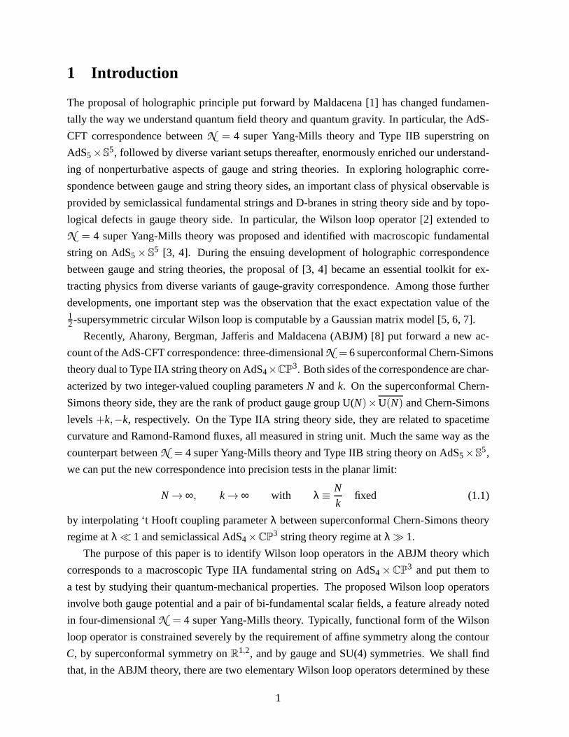
Figure 4:The diagrams of orderλ3 which vanish by themselves.

well with minimal surface result in string theory side. In the next section, we will take the same

assumption on vertex-type diagrams, utilize the above observation on skeleton propagators, and

propose a conjecture concerning circular Wilson loop in ABJM theory in terms of a Gaussian

matrix model.

The fourth diagram in fig. 2 is also encountered in the contextof pure Chern-Simons theory,

and its value is well-known [10]. We obtain

i2

NNλ2

16π

Z

τ1>τ2>τ3

x(τ1)l x(τ2)

mx(τ3)nεabcεlaiεmb jεnckIi jk =−π2λ2

6, (6.11)

where

Ii jk =

Z

d3x(x− x(τ1))

i(x− x(τ2))j(x− x(τ3))

k

|x− x(τ1)|3|x− x(τ2)|3|x− x(τ3)|3. (6.12)

We summarize the computations so far. For the timelike line,

〈WN[C,M]〉= 1+O(λ3). (6.13)

For the spacelike circle,

〈WN[C,M]〉=(

1+π2λ2+ · · ·)(

1− π2λ2

6+ · · ·

)+O(λ3). (6.14)

The first part is identical to the circular Wilson loop in four-dimensionalN = 4 super Yang-

Mills theory, while the second part is identical to the unknotted Wilson loop in pure Chern-

Simons theory.

21

Figure 5: The Feynman diagrams contributing to orderλ3. They all have two vertices of the

Wilson loop along the contourC.

6.3 W3[C]

We next analyze three-loop diagrams contributing toW3[C] and show that they all vanish.

Consider the timelike line first. All Feynman diagrams listed in fig. 4 vanish identically

because they are proportional to the supersymmetry conditions

TrM = 0 and TrM3 = 0, (6.15)

respectively.

For the Feynman diagrams in fig. 5, one easily finds that each ofthem vanish separately.

For instance, for the second to the last diagram, the skeleton two-loop integral is given by

1N

32π2TrM2 ·Nλ3 piεimn

Z

k,l

kmln

k2l2(k− p)2(k− l)2(l+ p− k)2 . (6.16)

Evidently, the two-loop integral should yield a result of the form:

A(p2)pm pn +B(p2)ηmn. (6.17)

22

Figure 6: The Feynman diagram at orderλ3 that vanish by itself. It has three vertices of the

Wilson loop along the contourC.

Figure 7:The Feynman diagrams at orderλ3 that cancel one another. They have three vertices

of the Wilson loop along the contourC.

Contracted withpiεimn, this contribution vanishes identically. Many of the diagrams in fig.

5 vanish because self-energy of scalars and fermions are zero at one-loop. For the Feynman

diagram in fig. 6, the contribution is proportional to

ε0mn pm1

Z

k

kn

k2(k− p1)2 = 0 (6.18)

so vanishes identically. The Feynman diagrams in fig. 7 cancel among themselves. To see this,

we need to manipulate loop integrals judiciously. For instance, although they contain a different

number of epsilon tensors and gauge boson propagators, nontrivial cancelation occurs between

the diagrams (2) and (3). The cancelation is possible because of various identities such as

(pm12 pm2

1 −ηm1m2 p1 · p2)ε0l1m1 pl11 ε0l2m2 pm2

2 = −p21p2

2+(non-covariant terms). (6.19)

Figure 8:The Feynman diagram at orderλ3 that vanish identically. It has four maximal vertices

of the Wilson loop along the contour.

23

In this way, two epsilon tensors cancel two gluon propagators in the diagram (2). It then cancels

the diagram (3). The non-covariant terms vanish after the contour integration, as we have seen

for two loop diagrams in subsection 6.2. Through judicious manipulations, one can show all

terms coming from the diagrams in fig. 7 cancel among themselves. We show details of the

cancelation in Appendix D.

The Feynman diagram 8 vanishes identically since it is proportional toε00m.

Consider next the spacelike circle case. Except the ones in fig. 7, all other Feynman dia-

grams vanish by the same reason as for the timelike line case,viz. either due to TrM = 0 or

due to contraction of momenta withεmnp tensor. After some manipulation, one also finds that

all Feynman diagrams in fig. 7 vanish. Start with the diagram (1). This gives a contribution

proportional toZ

τ1>τ2>τ3

xm1(τ1)xm2(τ2)x

m3(τ3)εm1l1k1εm2l2k2εm3l3k3Il1k1l2k2l3k3[x(τ1),x(τ2),x(τ3)], (6.20)

whereIl1k1l2k2l3k3[x(τ1),x(τ2),x(τ3)] consists of integrals over positions of the interaction ver-

tices. One can always choose two epsilon tensors in the integrand and replace them with a

sum of products ofηmns. Then, after carrying out the position integration, the integral should

contain terms with one epsilon tensor whose indices are contracted with (a derivative of)xm(τ).For instance, it produces a term like

xm1(τ1)xm2(τ2)x

m3(τ3)εm1m2m3 . (6.21)

For the spacelike circle, allxmi(τi)s lie onR2. Therefore, all the terms like (6.21) vanish iden-

tically. By the same argument, the diagram (2) must vanish. Moreover, this argument implies

that any Feynman diagram with odd number of epsilon tensors ought to vanish once the contour

integration is performed. Therefore, the diagrams (3) and (4) must vanish.

In summary, we find that three-loop contributionsW3[C] vanish for both the timelike line

case and the spacelike circle case.

6.4 Diagrammatical proof ofW2n+1[C] = 0

Drawing from the lower order computations, we emphasize again that the cancelation observed

among various Feynman diagrams is not specific to the ABJM theory. The same cancelation

would persist even for a theory with a generic number of matter flavor multiplet, so long as the

supersymmetry conditions TrM =TrM3 = 0 hold. In fact, up to the orderO(λ3), only the gauge

interaction vertices contributed to the Feynman diagrams.The quartet Yukawa interactions and

24

the sextet scalar interactions specific toN = 6 supersymmetric ABJM theory will only start to

contribute from the next order, viz. orderO(λ4). So, any result at orderO(λ4) or higher would

be considered as the discriminating test of the ABJM theory against any others.

In this subsection, we prove one result on higher order terms: W2n+1[C] = 0 for all n as

long as the contourC lies insideR2. In other words, the Wilson loop expectation value receives

nontrivial contribution only from even loop orders. Coincidentally, ABJM theory exhibits both

infrared and ultraviolet divergences only at even loop orders. Here, however, we are considering

not just these infinities but also finite parts. We begin with the observation that any Feynman

diagram can be drawn through the following two steps:

1. First, draw matter lines only. These diagrams need not be connected.

2. Next, add gluon lines.

In our proof, we shall follow these steps. First, we show thatthe diagrams with odd power of

λ vanish if there is no gluon propagator. Then, by counting number ofλs and theεmnp tensors as

a single gluon propagator is added to a given diagram, we prove inductively thatW2n+1[C] = 0.

Denote byvn the number ofn-valent vertices in a given diagramD. Herev1 is the number

of Am insertions from the Wilson loop, andv2 is the number ofYY † insertions from the Wilson

loop. Evidently, the numberI of internal lines is

I =12

6

∑n=1

nvn. (6.22)

The powerNk of λ is given as

Nk = I −6

∑n=3

vn

=12(v1+2v2)+

12

6

∑n=3

(n−2)vn. (6.23)

6.4.1 No gluon line

If there is no gluon line inD, then the non-zero numbers arev2, v4 (Yukawa coupling) andv6

(scalar potential). In this case,

Nk = v2+ v4+2v6. (6.24)

Due to the supersymmetry conditions of the velocity matrixMIJ, v2 must be even in any non-

vanishing diagram. Then we find thatv4 determines whetherNk is even or odd.

25

Fermions must appear inD as non-intersecting loops. Let

v4 = ∑ni (6.25)

be a partition ofv4. For eachni, there is a fermion loop which consists ofni fermion propagators.

Since Yukawa terms do not contain gamma matrices, each loop has the trace ofni gamma

matrices coming from the propagators. Ifni is odd, then the loop provides the epsilon tensor.

Therefore, ifv4 is odd, then there must be odd number of epsilon tensors. We already proved

that such diagram vanishes. This shows thatWNk=2n+1[C] = 0 if there is no gluon line.

6.4.2 Adding gluon lines

We have shown that, if there is no gluon line, thenNk and the numberNε of epsilon tensors are

equivalent modulo 2. If we can show that theNk ≡ Nε mod 2 holds whenever a gluon line is

added to a given diagramD which already satisfies that relation, then it provesW2n+1[C] = 0 in

general by induction. The above statement can be show to be true case by case. For example, if

a gluon line is added which connects two matter lines, then the number of vertices increases by

two, the number of propagators increases by three, which results in the increase ofNk by one,

and one epsilon tensor comes from the gluon line. Therefore,Nk ≡ Nε mod 2 still holds.

There might be one subtle point in this argument. Suppose that we have a generic diagram,

and eliminate all the gluon lines. Then the resulting diagram may contain a matter loop without

any vertex, that is, there could be a matter loop to which onlygluons are attached. Such a loop

is not included in the discussion given in the previous subsection. It seems that this causes no

problem since the matter loop in question does not give nok nor epsilon tensor. This can be

checked by considering a particular diagram with such a loopand eliminate the gluon lines.

Summarizing, we proved thatW2n+1[C] = 0 to all orders in perturbation theory. Note that

the necessary ingredients for the proof are (1) TrM2n+1 = 0, (2)C lies inR2 ∈ R4, and (3) the

action is classically conformally invariant so that the interaction terms consist only of gauge,

quartic Yukawa and sextet scalar couplings. It should be noted that our proof is insensitive to

specific value of the coefficients for each terms in the Yukawacouplings and the scalar potential.

7 Reduction to the Gaussian Matrix Model

In this section, we revisit planar perturbative evaluationof the circular Wilson loop. As demon-

strated in the previous section, expectation value of the circular Wilson loopWN[C,M] contains

26

features similar to the circular Wilson loop of 4-dimensional N = 4 super Yang-Mills theory

[5]. The first feature is that, apart from quantum corrections to gauge and scalar propagators, all

other diagrams vanish. Second feature is that sum of quantumcorrected gauge and scalar prop-

agators is reduced to a constant up to total derivative term.It is remarkable that these features

persists despite field contents, interactions and even spacetime dimensions are different between

the two conformal field theories. A new feature that arose forthe ABJM theory was that there is

an extra contribution from Chern-Simons interactions. Combining all these features, we expect

that expectation value of a circular ABJM Wilson loop computed in planar perturbation theory

can be brought into the form

〈WN[C,M]〉= 〈WN[C]〉CS〈WN[C,M]〉ladder. (7.1)

Here,〈WN[C]〉CSdenotes expectation value of an unknotted Wilson loop inpureChern-Simons

theory, while〈WN[C,M]〉ladder is the ladder part9 of the Wilson loop in the ABJM theory.

In this section, we employ the factorized form (7.1) as an ansatz, and explore possible exact

results concerning the Wilson loop.

7.1 Gaussian Matrix Model

In extracting Gaussian matrix model, our starting point will be the following assumptions.

• The two point function of gauge boson+scalar bilinear is a constant.

• The Wilson loop has the structure (7.1). All other diagrams than those in (7.1) cancel

each other and do not contribute to the expectation value.

These assumptions are actually true up to the order ofO(λ3), as we have demonstrated in the

previous section.

Let us first consider the ladder part. In the planar limit, by large-N factorization, expectation

value〈WN[C,M]〉 is given by

〈WN[C,M]〉= 〈WN[C,M]〉= 〈W N[C,M]〉. (7.2)

Parallel toN = 4 super Yang-Mills theory [5], we now show that〈WN[C,M]〉ladder can be

related to the Gaussian matrix model, but with an interesting twist.

Consider the Wilson loop onR3 and recall the exponentialΦ(τ)

Φ(τ) := [iAm(x)xm(τ)+MI

J(YIY †

J )(x)]x=x(τ). (7.3)

9This means ladders of quantum corrected propagators.

27

This Φ(τ) is in adjoint ofU(N), so we expanded it in the basis of Lie algebra generatorsT a:

Φ(τ) = Φa(τ)Ta. (7.4)

From the assumption, the two point function ofΦ is a constant. This is supported by the two

loop result (6.10):

〈Φa(τ1)Φb(τ2)〉=δab

Nf (λ) =

δab

N(λ2+O(λ4)). (7.5)

Therefore, contribution to the Wilson loop expectation value from ladder diagrams of quantum

correctedΦa propagators is obtainable from

〈WN[C,M]〉ladder=1N

∞

∑n=0

Z

τ1>τ2>···>τn

Tr [Ta1 . . .Tan ]〈Φa1(τ1) . . .Φan(τn)〉ladder. (7.6)

By the assumption, the integrands in the above equation areτ independent, soτ integral just

yield angular volume as

〈WN[C,M]〉ladder=1N

∞

∑n=0

1n!(2π)n Tr [Ta1 . . .Tan ]〈Φa1 . . .Φan〉ladder. (7.7)

Here, the expectation values〈· · · 〉ladderare evaluated according to the Wick’s theorem using the

propagator (7.5). We now rewrite the above series in a simpler form. IntroduceN2 real variables

Xa and the Gaussian integral〈F(X)〉mm for a functionF(X) as

〈F(X)〉mm :=1Z

Z

dN2X F(X)exp

[−1

2N

(2π)2 f (λ)∑a

XaXa], (7.8)

Z :=Z

dN2X exp

[−1

2N

(2π)2 f (λ)∑a

XaXa]. (7.9)

The Wick contracted expectation values can be replaced by the Gaussian integral. This brings

(7.7) to the form

〈WN[C,M]〉ladder=1N

∞

∑n=0

1n!

Tr [Ta1 . . .Tan ]〈Xa1 . . .Xan〉mm

=

⟨1N

Tr(eX)

⟩

mm, (7.10)

where we introduced a single Hermitian matrixX := XaTa. The Gaussian integral (7.8) can then

be rewritten as a Gaussian matrix integral:

〈F(X)〉mm=1Z

Z

dN2X F(X)exp

[− N(2π)2 f (λ)

Tr(X2)

]. (7.11)

28

In the planar limit, the expectation value (7.10) can be evaluated in terms of modified Bessel

functionI1 as

〈WN[C,M]〉ladder=

⟨1N

Tr(eX)

⟩

mm=

1

π√

2 f (λ)I1(2

√2π

√f (λ)). (7.12)

In the largef (λ) limit, we obtain asymptote of the Wilson loop expectation value as

〈WN[C,M]〉ladder∼ exp(2√

2π√

f (λ)) (7.13)

up to computable pre-exponential factors. If largef (λ) limit is also largeλ limit, this is a

prediction of the ABJM theory that could be compared with thestring theory dual.

7.2 Chern-Simons Contribution

In ABJM theory, the Wilson loop expectation value (7.1) contains an additional contribution

from pureChern-Simons interactions. We need to examine largef (λ) limit of this contribution

as well. By assumption we take〈WN[C]〉CS is the same as unknotted Wilson loop expectation

value in pure Chern-Simons theory. Exact answer of the latter is known [9]:

〈WN[C]〉CS=1N

qN2 −q−

N2

q12 −q−

12

, q := exp

(2πi

k+N

). (7.14)

In the ’t Hooft limit, this becomes

〈WN[C]〉CS=1+λ

πλsin

πλ1+λ

. (7.15)

We see that largeλ asymptote is given by

〈WN[C]〉CS= (λ−1+ . . .). (7.16)

We see that this contribution yields exponentially small corrections compared to the ladder

diagram contribution (7.13). Theλ−1 asymptote still carries an interesting information, sinceit

changes leading power ofλ in the pre-exponential. In particular, this indicates thatnumber of

zero-modes of the string worldsheet configuration dual to the circular Wilson loop in the ABJM

theory is different from that in theN = 4 super Yang-Mills theory.

7.3 Interpolation between Weak and Strong Coupling

By AdS/CFT correspondence, largeλ behavior ofWN[C,M] was determined from minimal sur-

face configuration of the string worldsheet in section 2. On the other hand, smallλ behavior of

29

WN[C,M] was determined from planar perturbation theory in section 6. This poses an interest-

ing question: what kind of functionf (λ) can interpolate between the weak and strong coupling

behavior? We assume that (7.12) can be used for this purpose with a suitable choice off (λ).The smallλ behavior off (λ) can be obtained by comparing (7.5) with (6.10), and the result is

already given in (7.5).Assumingthat largeλ limit is also largef (λ) limit, the largeλ behavior

can be extracted by comparing (7.13) with (2.1). We obtain

f (λ)→

λ2 (λ → 0)

λ4

(λ → ∞)

. (7.17)

When comparing various physical observables at weak coupling limit from the ABJM theory

and at strong coupling limit from the AdS4×CP3 string theory, various interpolating functions

analogous tof (λ) were introduced. An interesting question is whether some ofthese interpo-

lating functions are actually the same one. To test this possibility, consider the interpolating

function f (λ) introduced in the context of the giant magnon spectra [30, 35, 36]. There, it was

noted that dispersion relation of AdS4 giant magnon takes exactly the same form as that of AdS5

giant magnon except thatN = 4 super Yang-Mills ‘t Hooft couplingg2N is now replaced by

a nontrivial interpolating functionh(λ) of the N = 6 superconformal Chern-Simons ‘t Hooft

coupling:

g2N∣∣∣SYM

→ 16πh2(λ)∣∣∣ABJM

. (7.18)

At weak coupling,h(λ) ∼ λ. So, it is encouraging that the interpolating function associated

with the giant magnon and the interpolating function associated with the circular Wilson loop

are relatable each other ash2(λ) = f (λ). But it seems this would not work for all coupling

regime becauseh(λ) actually interpolates as

h(λ)→

λ (λ → 0)√

λ2

(λ → ∞) .

(7.19)

We see that it behaves differently at the strong coupling regime, so the two interpolating func-

tions are not identifiable. Our proposal of the Gaussian matrix model suggests that there ought

to be an independent interpolating functionf (λ) specific to the circular Wilson loop observ-

able. Sincef (λ) summarizes all-order corrections to the vacuum polarization of the ABJM

gauge fields, interpolating functions that would enter static quark potential or total cross section

of 2-body boson or fermion matter might be related tof (λ). It would be very interesting to

clarify the relation, if any, and compute higher order termsof f (λ).

30

8 Discussions

In this section, we discuss several interesting issues leftfor future investigation.

We identified an elementary Wilson loopWN[C,M] which transforms correctly under gener-

alized time-reversal, and we proposed that this is dual to fundamental Type IIA string. Though

the identification is correct from the viewpoint of charge conservation and time-reversal sym-

metry, consideration of other symmetries remains to be understood better. For the Wilson loop,

there exists a unique supersymmetric configuration and it preserves16 of theN = 6 superconfor-

mal symmetry. On the other hand, the fundamental string in AdS4 preserves12 supersymmetry.

Related, the supersymmetric Wilson loop preserves SU(2)×SU(2) subgroup of the SU(4) R-

symmetry, while the supersymmetric fundamental string in AdS4 preserves SU(3) subgroup.

We also observed that string configuration preserving16 supersymmetry and SU(2) subgroup is

obtainable by smearing string position inCP3 over aCP1. Still, given that a fundamental string

preserving12 supersymmetry and SU(3) subgroup of SU(4) R-symmetry exists, a supersymmet-

ric Wilson loop with the same symmetry is yet to be identified.

With the Wilson loop and its holographic dual is identified, various physical observables are

computable. By inspection, static quark potential at conformal point is exactly the same as AdS5

andN = 4 super Yang-Mills counterpart. It would be interesting to extend the computation to

Coulomb branch and compared the two sides. Also, various lightlike Wilson loops and their

cusp anomalous dimensions can be computed. It would be interesting to see if they are related

to scattering amplitudes and the fermionic T-duality of theABJM theory.

Another important direction is to compute theO(λ4) contribution to the circular Wilson

loop. The computation will elucidate validity of the factorization hypothesis of the Wilson loop

expectation value in terms of Gaussian matrix model proposed in section 7. The computation

is also a nontrivial test ofN = 6 supersymmetry since, from this order, Feynman diagrams

involving Yukawa coupling and sextet scalar interactions specific to the ABJM theory begin to

contribute. So we could find some distinguished features ofN = 6 ABJM model fromN = 2

superconformal Chern-Simons models. At the same time checking the cancellation is highly

non-trivial interesting problem. InN = 4 super Yang-Mills case, the reduction from circular

Wilson loop to the Gaussian matrix model is proved using localization[7]. Similar derivation

for the circular Wilson loop in the ABJM theory is also an interesting problem.

We intend to report progress of these issues in forthcoming publications.

31

Acknowlegement

We are grateful to Fernando Alday, Dongsu Bak, Lance Dixon, Andreas Gustavsson and Juan

Maldacena for enlightening discussions on issues related to this work. We also acknowledge

pertinent conversations with Dongmin Gang, Eunkyung Koh and Jaesung Park. This work was

supported in part by SRC-CQUeST-R11-2005-021, KRF-2005-084-C00003, EU FP6 Marie

Curie Research & Training Networks MRTN-CT-2004-512194 and HPRN-CT-2006-035863

through MOST/KICOS and F.W. Bessel Award of Alexander von Humboldt Foundation (SJR).

A Notation, Convention and Feynman Rules

A.1 Notation and Convention

• R1,2 metric:

gmn = diag(−,+,+) with m,n = 0,1,2.

ε012=−ε012=+1

εmpqεmrs =−(δpr δq

s −δps δq

r ); εmpqεmpr =−2δqr

(A.1)

• R1,2 Majorana spinor and Dirac matrices:

ψ ≡ two-component Majorana spinor

ψα = εαβψβ, ψα = εαβψβ where εαβ =−εαβ = iσ2

γmα

β = (iσ2,σ3,σ1), (γm)αβ = (−I,σ1,−σ3) obeying γmγn = gmn − εmnpγp.(A.2)

A.2 ABJM Theory

• Gauge and global symmetries:

gauge symmetry : U(N)·U(N)

global symmetry : SU(4) (A.3)

We denote trace over U(N) andU(N) as Tr andTr, respectively. We also denote generators

for U(N) andU(N) gauge groups by the same notationT a,(a = 0,1, · · · ,N2− 1). They are

Hermitian and normalized to

Tr(T aT b) =12

δab. (A.4)

32

• On-shell fields are gauge fields, complexified Hermitian scalars and Majorana spinors

(I = 1,2,3,4):

Am : Adj (U(N)); Am : Adj U(N)

Y I = (X1+ iX5,X2+ iX6,X3− iX7,X4− iX8) : (N,N;4)

Y †I = (X1− iX5,X2− iX6,X3+ iX7,X4+ iX8) : (N,N;4)

ΨI = (ψ2+ iχ2,−ψ1− iχ1,ψ4− iχ4,−ψ3+ iχ3) : (N,N;4)

Ψ†I = (ψ2− iχ2,−ψ1+ iχ1,ψ4+ iχ4,−ψ3− iχ3) : (N,N;4) (A.5)

• action: To suppress the cluttering 2π factors, we use the notationκ := k2π .

I = κZ

R1,2

[εmnpTr

(12

Am∂nAp +i3

AmAnAp

)− εmnpTr

(12

Am∂nAp +i3

AmAnAp

)

+12

Tr(−(DmY )†

I DmY I + iΨ†ID/ΨI

)+

12

Tr(−DmY I(DmY )†

I + iΨID/Ψ†I)

−VF−VB

](A.6)

Here, covariant derivatives are defined as

DmY I = ∂mY I + iAmY I − iY IAm , DmY †I = ∂mY †

I + iAmY †I − iY †

I Am (A.7)

and similarly for fermionsΨI,Ψ†I. Potential terms are

VF = iTr[Y †

I Y IΨ†JΨJ −2Y †I Y JΨ†IΨJ + εIJKLY †

I ΨJY †KΨL]

− iTr[Y IY †I ΨJΨ†J −2Y IY †

J ΨIΨ†J + εIJKLY IΨ†JY KΨ†L]

(A.8)

and

VB = −13

Tr[

Y †I Y JY †

J Y KY †KY I +Y †

I Y IY †J Y JY †

KY K

+4Y †I Y JY †

KY IY †J Y K −6Y †

I Y IY †J Y KY †

KY J]

(A.9)

At quantum level, since the Chern-Simons term shifts by integer multiple of 8π2, not onlyN but

alsok should be integrally quantized. At largeN, we expand the theory and physical observables

in double series of

gst =1N, λ =

Nk=

N2πκ

(A.10)

by treating them as continuous perturbation parameters.

33

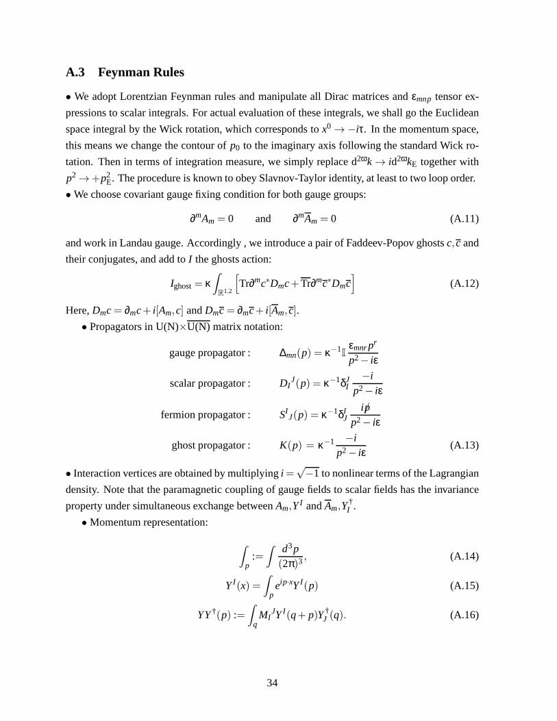
A.3 Feynman Rules

• We adopt Lorentzian Feynman rules and manipulate all Dirac matrices andεmnp tensor ex-

pressions to scalar integrals. For actual evaluation of these integrals, we shall go the Euclidean

space integral by the Wick rotation, which corresponds tox0 →−iτ. In the momentum space,

this means we change the contour ofp0 to the imaginary axis following the standard Wick ro-

tation. Then in terms of integration measure, we simply replace d2ωk → id2ωkE together with

p2 →+p2E. The procedure is known to obey Slavnov-Taylor identity, atleast to two loop order.

• We choose covariant gauge fixing condition for both gauge groups:

∂mAm = 0 and ∂mAm = 0 (A.11)

and work in Landau gauge. Accordingly , we introduce a pair ofFaddeev-Popov ghostsc,c and

their conjugates, and add toI the ghosts action:

Ighost= κZ

R1,2

[Tr∂mc∗Dmc+Tr∂mc∗Dmc

](A.12)

Here,Dmc = ∂mc+ i[Am,c] andDmc = ∂mc+ i[Am,c].

• Propagators in U(N)×U(N) matrix notation:

gauge propagator : ∆mn(p) = κ−1I

εmnr pr

p2− iε

scalar propagator : DIJ(p) = κ−1δJ

I−i

p2− iε

fermion propagator : SIJ(p) = κ−1δI

Jip/

p2− iε

ghost propagator : K(p) = κ−1 −ip2− iε

(A.13)

• Interaction vertices are obtained by multiplyingi=√−1 to nonlinear terms of the Lagrangian

density. Note that the paramagnetic coupling of gauge fieldsto scalar fields has the invariance

property under simultaneous exchange betweenAm,Y I andAm,Y†I .

• Momentum representation:

Z

p:=

Z

d3p(2π)3 , (A.14)

Y I(x) =Z

peip·xY I(p) (A.15)

YY †(p) :=Z

qMI

JY I(q+ p)Y †J (q). (A.16)

34

B Supersymmetry condition for generic contour

Consider the generalized supersymmetry conditions for theWilson loop:

ξIJn/(τ)+MIK(τ)iξKJ = 0. (B.1)

We assume thatn(τ)2 =−1 andMIJ(τ) is a hermitian matrix.M(τ) can be decomposed as

M(τ) =U†(τ)Λ(τ)U(τ), (B.2)

whereΛ(τ) = Λ is a constant diagonal matrix unlessU(τ) is allowed to have discontinuities.

We assume thatU(τ) is continuous, andΛ = diag(−1,−1,+1,+1) so that the generalized

supersymmetry conditions have a non-trivial solution.

Let us assume, without loss of generality, thatU(τ = 0) is the identity matrix. Then, non-

zero components ofξIJ areξ12 andξ34 with

ξ12n/= iξ12, ξ34n/=−iξ34, (B.3)

wherenm = nm(0). Define

ξIJ(τ) :=U(τ)IKξKJ. (B.4)

Notice thatξIJ(τ) is no longer anti-symmetric. This satisfies

ξIJ(τ)n/(τ)+ΛIK(τ)iξKJ(τ) = 0. (B.5)

Sincenm(τ) is related tonm by a Lorentz transformationLml(τ), we find its spinor representation

S(τ)γmS−1(τ) = γmLml(τ)nl, (B.6)

with S(0) = 1 by definition. Now the supersymmetry condition becomes

ξIJ(τ)S(τ)n/+ΛIKiξKJ(τ)S(τ) = 0. (B.7)

Consider the following condition:

ξ13(τ)S(τ)n/− iξ13(τ)S(τ) = 0 (B.8)

for a genericτ. Sinceξ13(τ) =U14(τ)ξ43, this condition implies

U14(τ) = 0 or ξ34S(τ)n/− iξ34S(τ) = 0. (B.9)

As long as the contour is smooth, that is,S(τ) is continuous, the latter contradicts with (B.3).

Therefore, we conclude thatU14(τ) = 0 holds. Using similar arguments, one can show that

U(τ) =

u1(τ) 0

0 u2(τ)

, (B.10)

whereu1(τ),u2(τ) areU(2) matrices. This immediately implies thatM(τ) = Λ andnm(τ) = nm.

35

C Vacuum polarization

The self-energy correction enters in the same form for the U(N) and theU(N) gauge fields.

Therefore we focus on the correction toA gauge field only. At the one-loop level, the boson,

the fermion, the gauge and the ghost loops may in general contribute to the gauge self-energy

correction. In this appendix, we identify these self-energy contributions.

We begin with the scalar loop contribution. It is the sub-diagram of Fig. 3. The momentum

k plays the role of the external momentum. The self energy contribution reads

iΠsab(k) = (i)2[i ]2(4)i

Z

d2ωℓ

(2π)2ω(2ℓ+ k)a(2ℓ+ k)b

(k+ ℓ)2 ℓ2 , (C.1)

where the extra factor 4 comes from the fact that 4 complex scalars are coupled to the gauge

field. Using the dimensional regularization, one obtains

iΠsab(k) = (4)i

[kakb −gabk2

16k

]. (C.2)

Similarly, for the fermion loop, the self-energy contribution becomes

iΠ fab(k) = (i)2[i ]2(4)(−)FD i

Z

d2ωℓ

(2π)2ωtrγa (ℓ/+ k/)γb ℓ/

(k+ ℓ)2 ℓ2 , (C.3)

where again the extra factor four comes from the fact that there are 4 complex fundamental

fermions. Using theγ matrix identity and the dimensional regularization, the contribution be-

comes

iΠ fab(k) = (4)i

[kakb −gabk2

16k

]. (C.4)

Hence, each complex matter contributes by the same weight and sign.

One can continue the dimensions 2ω to four and obtain the vacuum polarization in four-

dimensional Yang-Mills theories. The integration leads tothe logarithmic divergence in this

case contributing positively to theβ-function of the Yang-Mills coupling. Again, boson and

fermion contributions add up.

For the gluon self-energy contribution, we have

iΠAab(k) = (3) · (3)[i2]

[ iκ3

]2[1κ

]2(i)2[i ]2(4)i

Z

d2ωℓ

(2π)2ωεmbnε jaiεimqεn jr(ℓ+ k)qℓr

(k+ ℓ)2 ℓ2 ,

= iZ

d2ωℓ

(2π)2ω(ℓ+ k)aℓb +(ℓ+ k)bℓa

(k+ ℓ)2 ℓ2 . (C.5)

It becomes

iΠAab(k) =−i

[kakb +gabk2

32k

], (C.6)

36

which alone does not respect the gauge invariance. However,there exists also the ghost loop

contribution,

iΠghab(k) = (i)2[i ]2(−)i

Z

d2ωℓ

(2π)2ω(ℓ+ k)aℓb +(ℓ+ k)bℓa

(k+ ℓ)2 ℓ2 , (C.7)

where we put the extra (−) sign due to the ghost statistics. Therefore, the ghost contribution

cancels out precisely the gauge loop contribution, reproducing the well-established result [34].

Again, analytically continuing to four dimensions, the integral expression for the gauge part

changes while the ghost integral remains intact. With Yang-Mills couplings, both contributions

no longer cancel each other but contribute negatively to theβ-function.

D Feynman integrals for 3-loop diagrams in figure 7

The diagram (2) provides

−32π3λ3Em1m2m3

Z

k

1k2(k− p1)2(k− p1− p2)2

[T m1m2m3

F1 +T m1m2m3F2 +T m1m2m3

F3 +T m1m2m3F4

]

(D.1)

where we defined

Em1m2m3 =3

∏i=1

ε0limi plii

p2i

, (D.2)

and

T m1m2m3F1 = −8km1(k− p1)

m2km3, (D.3)

T m1m2m3F2 = −2(pm1

2 pm21 −ηm1m2 p1 · p2)k

m3 −2(pm23 pm3

2 −ηm2m3 p2 · p3)km1

−2(pm31 pm1

3 −ηm3m1 p3 · p1)(k− p1)m2 (D.4)

T m1m2m3F3 = 2pm1

3 pm21 pm3

2 − (ηm1m2 pm31 p2

3+ηm2m3 pm12 p2

1+ηm3m1 pm23 p2

2) (D.5)

T m1m2m3F4 = −

(ηm2m3km1[−k2− (k− p1− p2)

2]+ηm1m2km3[−(k− p1)2− (k− p1− p2)

2]

−ηm1m2(k− p1)m3[−k2− (k− p1− p2)

2]+ηm1m2km3[−k2− (k− p1)2]

−ηm2m3(k− p2)m1[−k2− (k− p1)

2]+ηm3m1(k− p1)m2[−k2− (k− p1− p2)

2]

−ηm3m1km2[−(k− p1)2− (k− p1− p2)

2]+ηm3m1(k− p1)m2[−k2− (k− p1)

2]

+ηm2m3km1[−(k− p1)2− (k− p1− p2)

2]). (D.6)

37

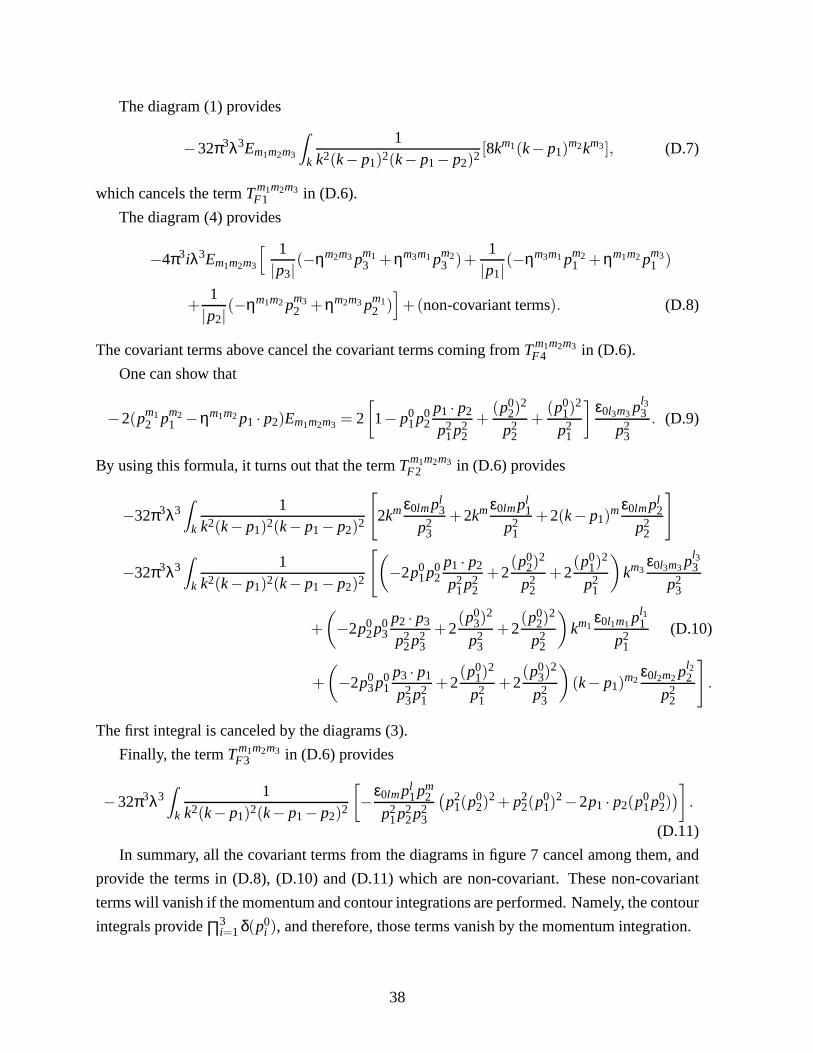
The diagram (1) provides

−32π3λ3Em1m2m3

Z

k

1k2(k− p1)2(k− p1− p2)2 [8km1(k− p1)

m2km3], (D.7)

which cancels the termT m1m2m3F1 in (D.6).

The diagram (4) provides

−4π3iλ3Em1m2m3

[ 1|p3|

(−ηm2m3 pm13 +ηm3m1 pm2

3 )+1

|p1|(−ηm3m1 pm2

1 +ηm1m2 pm31 )

+1

|p2|(−ηm1m2 pm3

2 +ηm2m3 pm12 )

]+(non-covariant terms). (D.8)

The covariant terms above cancel the covariant terms comingfrom T m1m2m3F4 in (D.6).

One can show that

−2(pm12 pm2

1 −ηm1m2 p1 · p2)Em1m2m3 = 2

[1− p0

1p02

p1 · p2

p21p2

2

+(p0

2)2

p22

+(p0

1)2

p21

]ε0l3m3 pl3

3

p23

. (D.9)

By using this formula, it turns out that the termT m1m2m3F2 in (D.6) provides

−32π3λ3Z

k

1k2(k− p1)2(k− p1− p2)2

[2km ε0lm pl

3

p23

+2km ε0lm pl1

p21

+2(k− p1)m ε0lm pl

2

p22

]

−32π3λ3Z

k

1k2(k− p1)2(k− p1− p2)2

[(−2p0

1p02

p1 · p2

p21p2

2

+2(p0

2)2

p22

+2(p0

1)2

p21

)km3

ε0l3m3 pl33

p23

+

(−2p0

2p03

p2 · p3

p22p2

3

+2(p0

3)2

p23

+2(p0

2)2

p22

)km1

ε0l1m1 pl11

p21

(D.10)

+

(−2p0

3p01

p3 · p1

p23p2

1

+2(p0

1)2

p21

+2(p0

3)2

p23

)(k− p1)

m2ε0l2m2 pl2

2

p22

].

The first integral is canceled by the diagrams (3).

Finally, the termT m1m2m3F3 in (D.6) provides

−32π3λ3Z

k

1k2(k− p1)2(k− p1− p2)2

[−ε0lm pl

1pm2

p21p2

2p23

(p2

1(p02)

2+ p22(p0

1)2−2p1 · p2(p0

1p02))]

.

(D.11)

In summary, all the covariant terms from the diagrams in figure 7 cancel among them, and

provide the terms in (D.8), (D.10) and (D.11) which are non-covariant. These non-covariant

terms will vanish if the momentum and contour integrations are performed. Namely, the contour

integrals provide∏3i=1 δ(p0

i ), and therefore, those terms vanish by the momentum integration.

38

References

[1] J. M. Maldacena, “The large N limit of superconformal field theories and supergrav-

ity,” Adv. Theor. Math. Phys.2 (1998) 231 [Int. J. Theor. Phys.38 (1999) 1113]

[arXiv:hep-th/9711200].

[2] K. G. Wilson, “Confinement of quarks,” Phys. Rev. D10 (1974) 2445.

[3] S. J. Rey and J. T. Yee, “Macroscopic strings as heavy quarks in large N gauge theory

and anti-de Sitter supergravity,” Eur. Phys. J. C22 (2001) 379 [arXiv:hep-th/9803001].

S. J. Rey, S. Theisen and J. T. Yee, “Wilson-Polyakov loop at finite temperature in

large N gauge theory and anti-de Sitter supergravity,” Nucl. Phys. B527 (1998) 171

[arXiv:hep-th/9803135].

[4] J. M. Maldacena, “Wilson loops in large N field theories,”Phys. Rev. Lett.80 (1998) 4859

[arXiv:hep-th/9803002].

[5] J. K. Erickson, G. W. Semenoff and K. Zarembo, “Wilson loops in N = 4 supersymmetric

Yang-Mills theory,” Nucl. Phys. B582(2000) 155 [arXiv:hep-th/0003055].

[6] N. Drukker and D. J. Gross, “An exact prediction of N = 4 SUSYM theory for string

theory,” J. Math. Phys.42 (2001) 2896 [arXiv:hep-th/0010274].

[7] V. Pestun, “Localization of gauge theory on a four-sphere and supersymmetric Wilson

loops,” arXiv:0712.2824 [hep-th].

[8] O. Aharony, O. Bergman, D. L. Jafferis and J. Maldacena, “N=6 superconformal Chern-

Simons-matter theories, M2-branes and their gravity duals,” arXiv:0806.1218 [hep-th].

[9] E. Witten, “Quantum field theory and the Jones polynomial,” Commun. Math. Phys.121

(1989) 351.

[10] E. Guadagnini, M. Martellini and M. Mintchev, “Wilson Lines in Chern-Simons Theory

and Link Invariants,” Nucl. Phys. B330(1990) 575.

[11] D. Berenstein and D. Trancanelli, “Three-dimensionalN=6 SCFT’s and their membrane

dynamics,” arXiv:0808.2503 [hep-th].

[12] S. Mukhi and C. Papageorgakis, “M2 to D2,” JHEP0805(2008) 085 [arXiv:0803.3218

[hep-th]].

39

[13] Y. Honma, S. Iso, Y. Sumitomo and S. Zhang, “Scaling limit of N=6 superconformal

Chern-Simons theories and Lorentzian Bagger-Lambert theories,” arXiv:0806.3498 [hep-

th].

[14] T. Li, Y. Liu and D. Xie, “Multiple D2-Brane Action from M2-Branes,” arXiv:0807.1183

[hep-th].

[15] Y. Pang and T. Wang, “From N M2’s to N D2’s,” arXiv:0807.1444 [hep-th].

[16] Y. Honma, S. Iso, Y. Sumitomo, H. Umetsu and S. Zhang, “Generalized Conformal Sym-

metry and Recovery of SO(8) in Multiple M2 and D2 Branes,” arXiv:0807.3825 [hep-th].

[17] J. Bagger and N. Lambert, “Gauge Symmetry and Supersymmetry of Multiple M2-

Branes,” Phys. Rev. D77 (2008) 065008 [arXiv:0711.0955 [hep-th]].

[18] A. Gustavsson, “Algebraic structures on parallel M2-branes,” arXiv:0709.1260 [hep-th].

[19] D. Bak and S. J. Rey, “Integrable Spin Chain in Superconformal Chern-Simons Theory,”

arXiv:0807.2063 [hep-th].

[20] N. Drukker, J. Plefka and D. Young, “Wilson loops in 3-dimensional N=6 supersymmetric

Chern-Simons Theory and their string theory duals,” arXiv:0809.2787 [hep-th].

[21] B. Chen and J. B. Wu, “Supersymmetric Wilson Loops in N=6Super Chern-Simons-

matter theory,” arXiv:0809.2863 [hep-th].

[22] J. Kluson and K. L. Panigrahi, “Defects and Wilson Loopsin 3d QFT from D-branes in

AdS(4) x CP**3,” arXiv:0809.3355 [hep-th].

[23] D. E. Berenstein, R. Corrado, W. Fischler and J. M. Maldacena, “The operator product

expansion for Wilson loops and surfaces in the large N limit,” Phys. Rev. D59 (1999)

105023 [arXiv:hep-th/9809188].

[24] N. Drukker, D. J. Gross and H. Ooguri, “Wilson loops and minimal surfaces,” Phys. Rev.

D 60 (1999) 125006 [arXiv:hep-th/9904191].

[25] K. Zarembo, “Supersymmetric Wilson loops,” Nucl. Phys. B 643 (2002) 157

[arXiv:hep-th/0205160].

[26] A. Dymarsky, S. S. Gubser, Z. Guralnik and J. M. Maldacena, “Calibrated surfaces and

supersymmetric Wilson loops,” JHEP0609(2006) 057 [arXiv:hep-th/0604058].

[27] S.-J. Rey, unpublished notes (2004, 2008); to appear.

40

[28] A. Miwa, “BMN operators from Wilson loop,” JHEP 0506 (2005) 050

[arXiv:hep-th/0504039].

[29] M. Fujita, “BPS operators from the Wilson loop in the 3-dimensional supersymmetric

Chern-Simons theory,” arXiv:0902.2381 [hep-th].

[30] D. Gaiotto, S. Giombi and X. Yin, “Spin Chains in N=6 Superconformal Chern-Simons-

Matter Theory,” arXiv:0806.4589 [hep-th].

[31] K. Hosomichi, K. M. Lee, S. Lee, S. Lee and J. Park, “N=5,6Superconformal Chern-

Simons Theories and M2-branes on Orbifolds,” arXiv:0806.4977 [hep-th].

[32] S. Terashima, “On M5-branes in N=6 Membrane Action,” JHEP 0808 (2008) 080

[arXiv:0807.0197 [hep-th]].

[33] D. Gaiotto and X. Yin, “Notes on superconformal Chern-Simons-matter theories,” JHEP

0708, 056 (2007) [arXiv:0704.3740 [hep-th]].

[34] W. Chen, G. W. Semenoff and Y. S. Wu, “Two loop analysis ofnonAbelian Chern-Simons

theory,” Phys. Rev. D46, 5521 (1992) [arXiv:hep-th/9209005].

[35] T. Nishioka and T. Takayanagi, “On Type IIA Penrose Limit and N=6 Chern-Simons The-

ories,” JHEP0808, 001 (2008) [arXiv:0806.3391 [hep-th]].

[36] G. Grignani, T. Harmark and M. Orselli, “The SU(2) x SU(2) sector in the string dual of

N=6 superconformal Chern-Simons theory,” arXiv:0806.4959 [hep-th].

41