Southern California Wind Event ­ A WES Case Study9­10 February 2002

BACKGROUND:

Strong offshore winds pose a significant threat to Southern Californians. These events occur ona fairly regular basis resulting in the usual downed trees and power lines, roof and signdamage, overturned 18­wheelers, extreme fire weather conditions, and, rarely, a fatality–usually due to someone coming in contact with downed power lines. Two types of high windproducing offshore wind events that have been particularly well documented are the Santa AnaWinds of Southern California and the Sundowner Winds of Santa Barbara.

In 1995, Ivory Small [SOO SGX] authored NOAA Technical Memorandum NWS WR­230 titledSanta Ana Winds and the Fire Outbreak of Fall 1993. In his memo, Ivory discussed severalconceptual models regarding the nature of Santa Ana winds, favored synoptic and mesoscalepatterns associated with Santa Ana wind events, and forecasting techniques used by localforecasters at the time. In 1996, Gary Ryan [DAPM at LOX] authored NOAA TechnicalMemorandum NWS WR­240, titled Downslope Winds of Santa Barbara, California, whichdescribed the strong Sundowner Winds that occur commonly below the passes and canyons ofthe Santa Ynez Mountains. Gary also discussed the synoptic patterns that favoredSundowners, some forecasting rules of thumb, and gave a brief history of significantSundowner events. Finally, in January 2000, a team of researchers at the National WeatherService Office in Oxnard [LOX], headed by Gary Ryan and Dave Bruno [Lead Forecaster],authored a second NOAA Tech Memo, NWS WR­261, titled Climate of Los Angeles, California.This document contained a diagram showing the three main Santa Ana wind corridors thatsurround the Los Angeles Basin–(1) the Santa Clara River Valley corridor through western LosAngeles County and southern Ventura County, (2) the Cajon Pass corridor that separates theSan Gabriel Mountains from the San Bernardino Mountains, and (3) the Banning Pass corridorthat runs east­west between the San Bernardino Mountains and the San Jacinto Range. As adirect result of these studies and other research, the anticipation of strong offshore wind eventsover Southern California is usually well forecast. However, critical details of the wind event suchas where, when and how strong it will be can be extremely difficult to determine.

INTRODUCTION:

The high wind event of 9­10 February 2002 was a fairly typical Southern California wind event.It began with strong northwest to north winds through and below passes and canyons of theSanta Ynez Range [Sundowner winds] and transitioned in about 24 hours to a Santa Ana windevent with northeasterly winds through and below the passes and canyons of the San GabrielMountains. From the base of the mountains the flow splits, either channeling through the SantaClara River Valley and offshore over the Oxnard Plain in Ventura County, or through the SanFernando Valley where it usually splits again to flow either through Simi Valley then the OxnardPlain, through the passes and canyons of the Santa Monica Mountains and Malibu, or simplythrough the Los Angeles Basin itself. The forecast challenge for these types of offshore windevent is not whether or not there was going to be a wind event; but rather, how strong an eventwould it be [advisory or warning?] and exactly where would the strongest winds occur?

There were several reasons why this particular event was chosen as a WES exercise.

1. As mentioned above, high wind events have a significant impact on Southern Californians.Therefore, it is very important that they be forecast accurately and with sufficient lead time.However, this was actually a marginal high wind event by Southern California standards.Therefore, it was not a slam dunk forecast; although it did result in widespread minor winddamage and one fatality due to a falling tree.

2. The fact that it was going to be windy on the 9th of February should not have been a surpriseto any Southern Californian. Wind advisories for the region had been issued the precedingafternoon at 3:10 PM. This was plenty of time for viewers of even the early edition eveningnews to get the word. However, wind warnings were not issued until the 9th at 8:45 AM–whichwas about the same time that winds increased to warning levels in the mountains. Thus, thewarning had insufficient lead time which made it a candidate for local forecast review. A WESExercise seemed the logical choice for the forecast review process. Not only would it directlyinvolve the participation of the entire forecast staff, but it would also give everyone a crack atimproving warning lead time for the event–assuming that the individual actually elected to issuea warning, of course.

3. The initial studies of offshore wind events by Ryan and Small were done back in the PC­GRIDS era. Today, AWIPS offers forecasters much better tools for slicing and dicing modeloutput to build displays of offshore winds and their critical forecast criteria. This WES Exercisespecifically suggested several of the key AWIPS displays to look at for evaluating offshore windevents in order to make a better warn/no­warn decision.

4. Finally, this event gave everyone the opportunity to re­familiarize themselves with some ofthe unique terrain aspects of the various locations favored by high winds [Fig 1]. As waspointed out above, high wind events have been well­documented for both Sundowner Winds inSanta Barbara County and Santa Ana Winds through the Santa Clarita River and SanFernando Valleys. However, there is a tendency for forecasters to overlook the less well­documented winds that occur through the Tejon Pass in Northern Los Angeles County [neitherSundowner nor Santa Ana]. The Tejon Pass winds commonly occur in transitions fromSundowner to Santa Ana winds. While much more localized, these winds and can besignificantly stronger than either the Sundowner or Santa Ana and can close the Grapevinesection of Interstate 5, thus seriously disrupting commerce and travel on the main route northfrom the LA Basin. Forecasters were specifically asked to evaluate the gradients through thispass during the WES Exercise.

SYNOPTIC FEATURES:

There was nothing particularly unusual in the synoptic pattern of this event. Following the usualscenario, a surface ridge of high pressure moved onshore over Central California on the 8th ofFebruary and was building over the Great Basin. Aloft, there was an upper level ridge buildingover the Eastern Pacific. By 1500Z on the morning of 9 February, just before the warning levelwinds kicked in, there was a 1045 mb surface high over Idaho and, aloft, there was a north­south oriented 500 mb ridge with a 586 center located about 600 miles southwest of LAX.There were three key aspects of this pattern that the forecasters had to evaluate.

1. First, were offshore surface pressure gradients strong enough to generate strong offshorewinds?

2. How well did the upper air pattern align with and support the low level winds?

3. Was the thermal structure of the atmosphere favorable for the downward transport of strongwinds aloft to the surface?

DISCUSSION:

The initial review of the missed warning indicated that the models had actually done a verygood job handling both the synoptic and mesoscale aspects of the event. Therefore, the eventoffered a particularly good opportunity to discuss the importance of evaluating the models andof monitoring the mesoscale data necessary for assessing the three major aspects of aSouthern California high wind event.

THE EXERCISE:

Due to limitations of the available archive, the forecast time period had to be artificiallytruncated. This truncation eliminated the possibility of forecasters ever achieving the desiredlead time of 8 hours. However, for the purposes of this exercise, it was still excellent trainingexercise for the forecast staff and provided everyone with the opportunity for improving on thelead time that was provided during the actual event. The exercise was in three parts.

1. Part 1 of the WES displaced real time [DRT] exercise "started" on a mid shift, about 1100 PM[0700Z] on Friday evening, the 8th of February. Forecasters were provided with the currentsituation–advisories in effect, an hour­by­hour history of the observed winds [ex. Fig 2], and thepressure gradient trends over the past 14 hours [Table 1]. The steps of this portion of theexercise were as follows:

a. Build a display on AWIPS similar to Figure 1 and then compare and contrast the differentwind corridors that lie along or parallel to the axes B­B1 [LAX­BFL] and C­C1 [LAX­DAG].

b. Compute the forecast wind gradients from the 09/06Z Meso­Eta model forecast for 06Z, 12Z,18Z, and 10/00Z [Fig 3, Fig 4, Fig 5, Fig 6].

c. Build a cross section along line A­A1, Point Mugu Naval Air Station to Lancaster [KNTD­KWJF] depicting Meso­Eta winds, wind speed, omega, and potential temperature [Fig 7a/7b,Fig 8a/8b]. [Note: Paired a/b displays used for clarity.]

d. Forecasters were then asked to comment on the cross section along with the Meso­EtaMSLP display and make a Warn/No­Warn decision regarding the need to upgrade the windadvisories to high wind warnings and indicate which zones would require upgrading.

2. For Part 2 of the exercise, the DRT clock was advanced to 1200Z and restarted. Additionalgradient trends were provided [Table 2] along with hour­by hour displays of the observed winds[ex. Fig 9]. Forecasters were asked how the Meso­Eta forecast gradients compared with thoseobserved in the intervening time period from 0700Z.

3. The final part of the exercise was a self­evaluation. Forecasters were given hourly winddisplays up until 11/03Z that evening. They were then asked to verify whether or not a warningwas required, for what zones, and they were asked to compute their own lead times, assumingthey had issued the required warnings.

CONCLUSION:

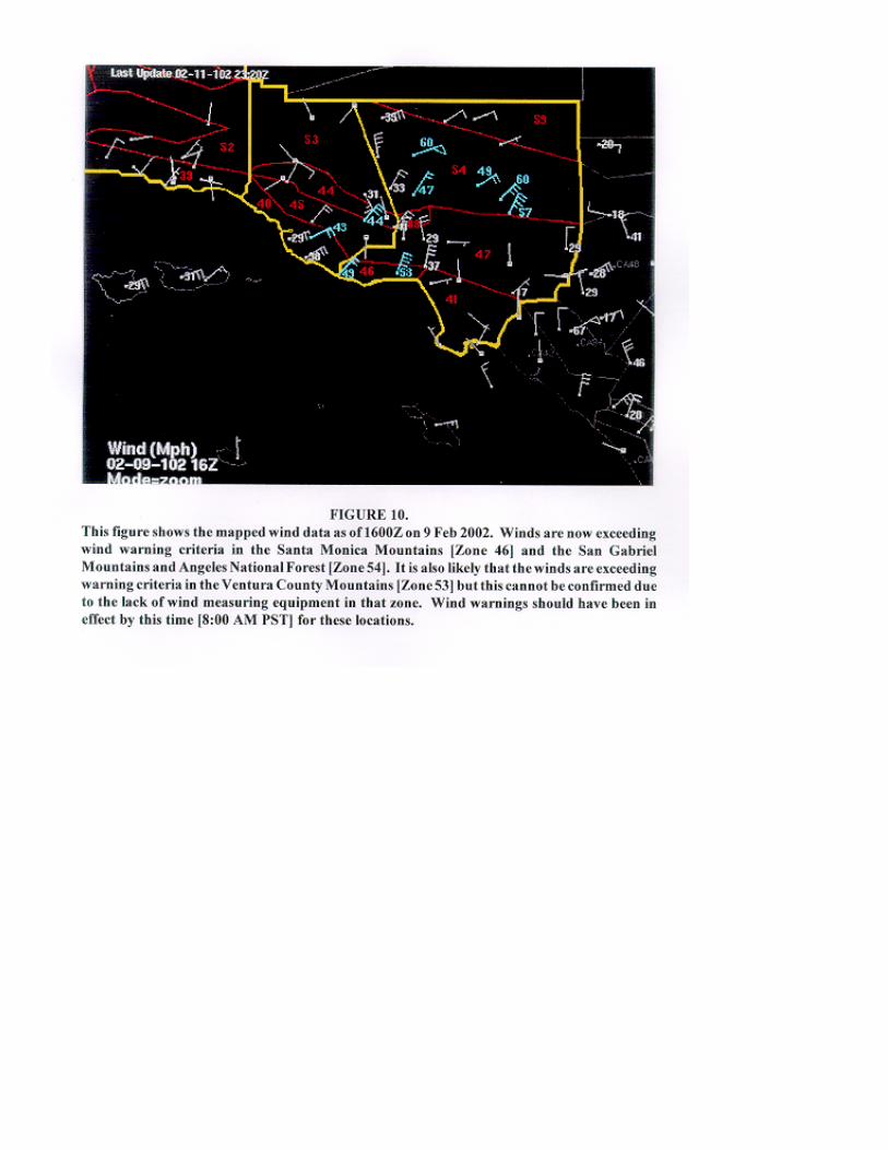
Each part of the exercise was accompanied by a worksheet with questions to be completed bythe forecaster. These worksheets [not shown] were used to evaluate each forecaster'sunderstanding of the event and their warning lead times, if any. As it turns out, warnings wererequired for two zones and probably a third. Figure 10 shows the mapped winds for 1600Z on 9Feb 2002. Accordingly, by this time winds have exceeded warning criteria in Zones 46 and 54,and probably in Zone 53; however, that could not be verified for sure due to lack of windsensors. The time of 1600Z was used as the time of occurrence for the lead time calculations.As the day went on, the winds increased and advisories verified in most of the adjacent zones;however, winds exceeded wind warning criteria in only the three zones mentioned above.

Table 1

Table 2

Figure 1

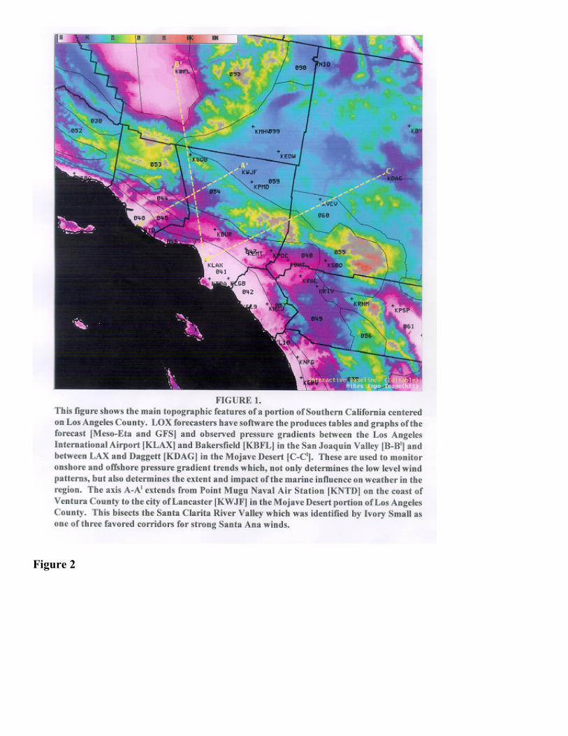
Figure 2

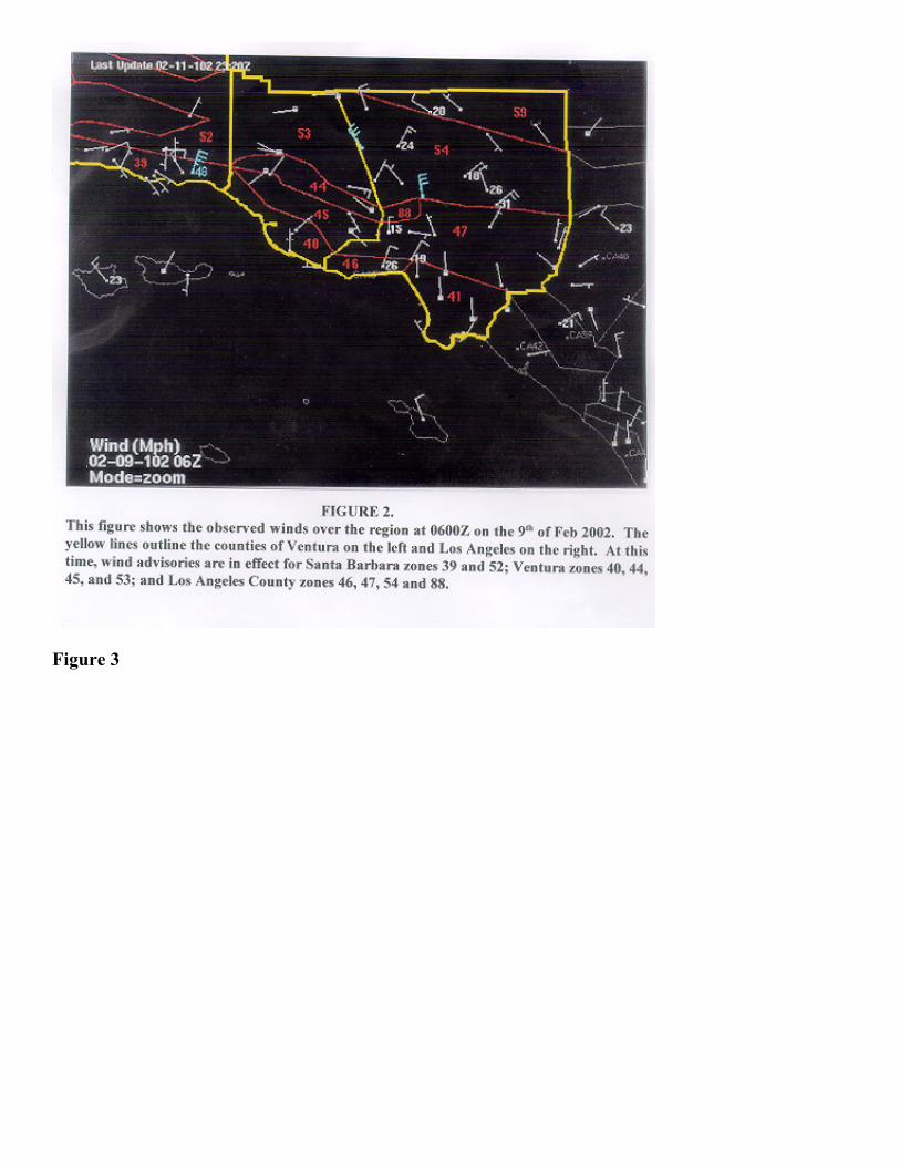
Figure 3

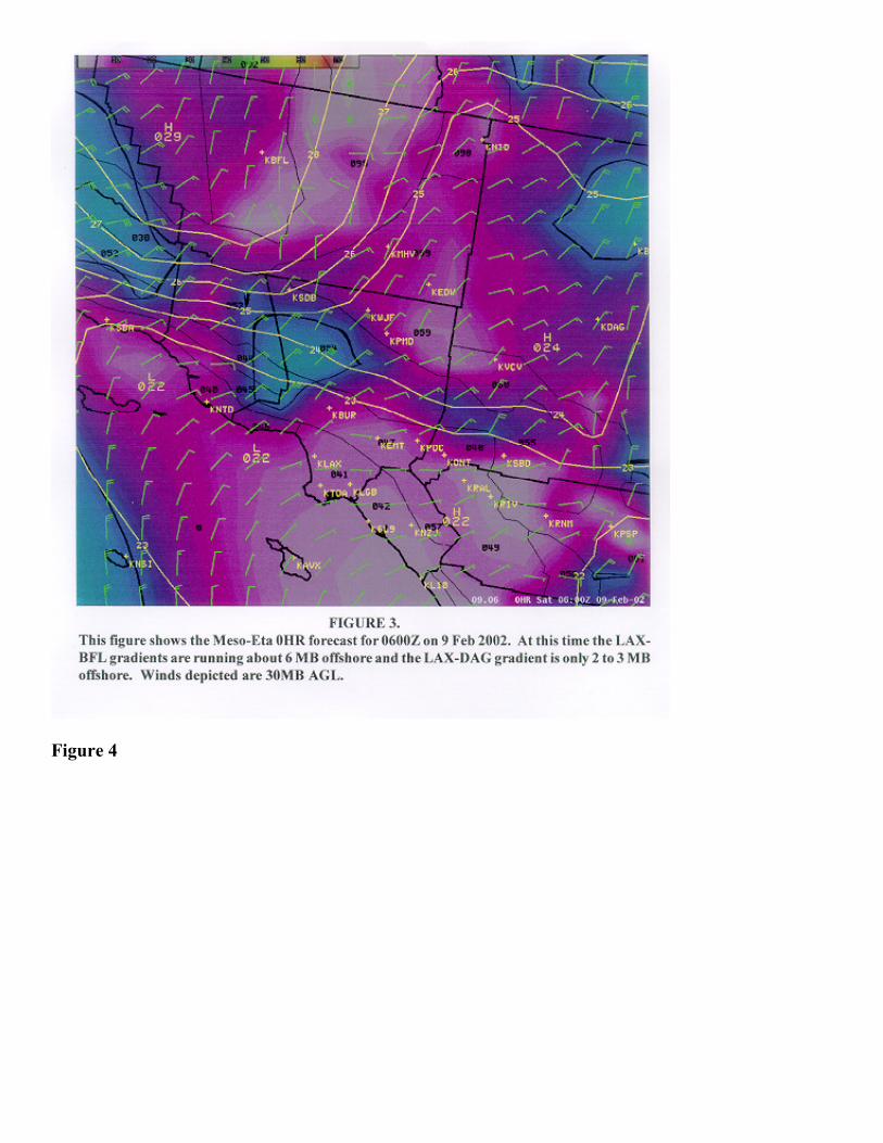
Figure 4

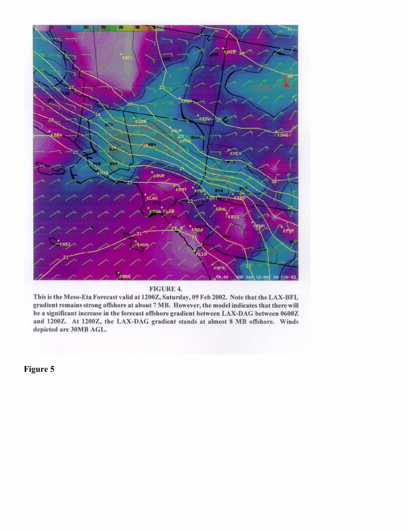
Figure 5

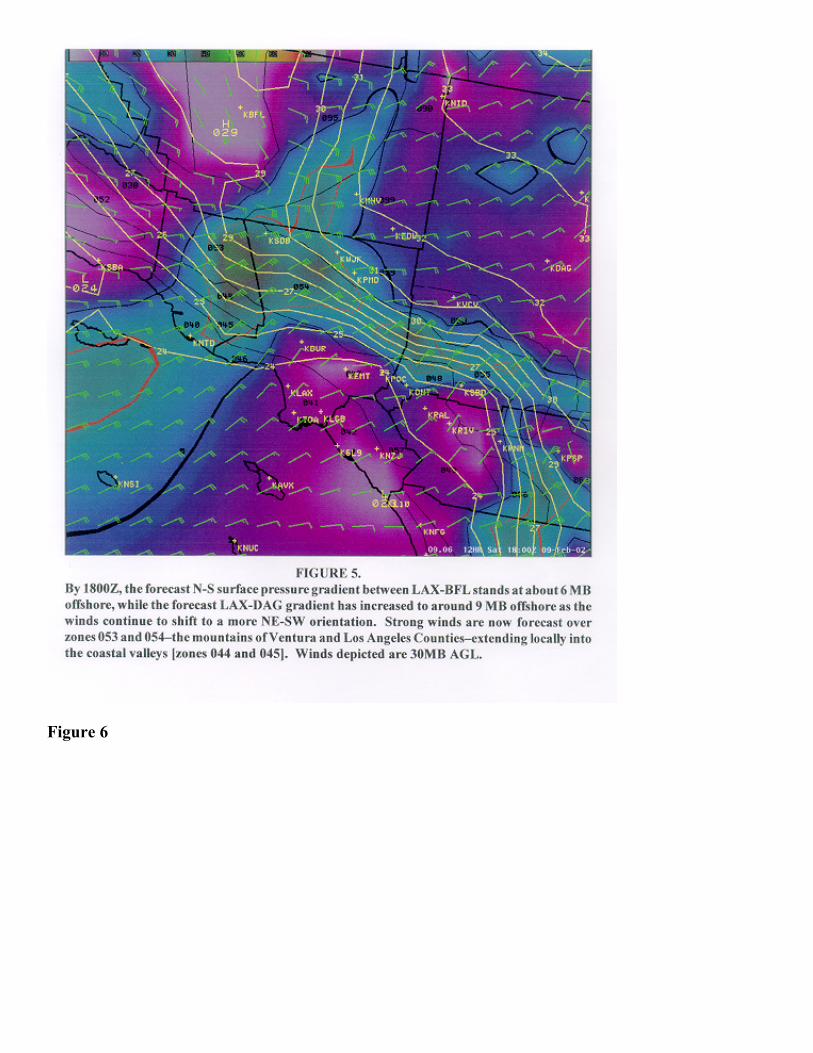
Figure 6

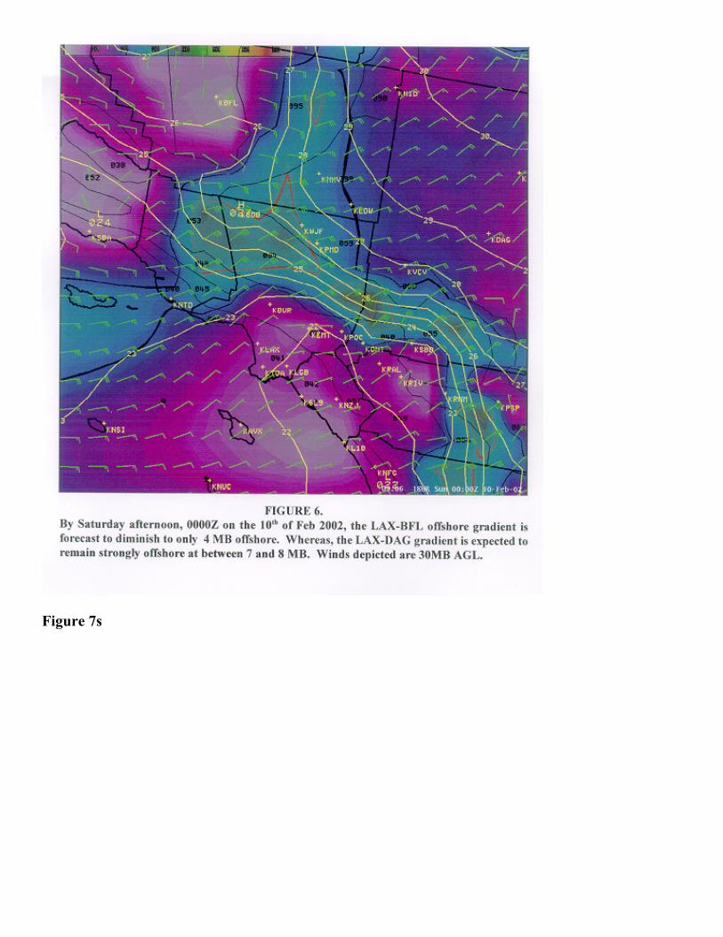
Figure 7s

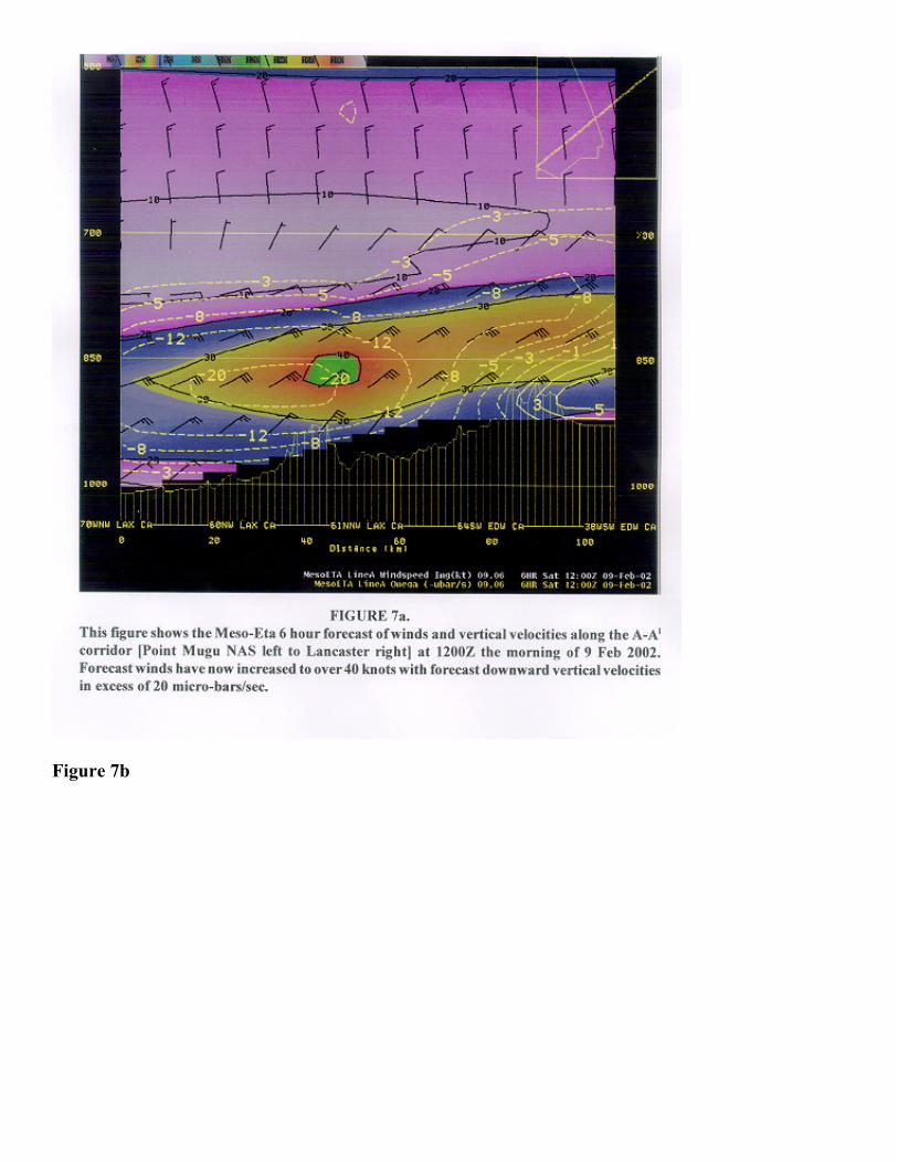
Figure 7b

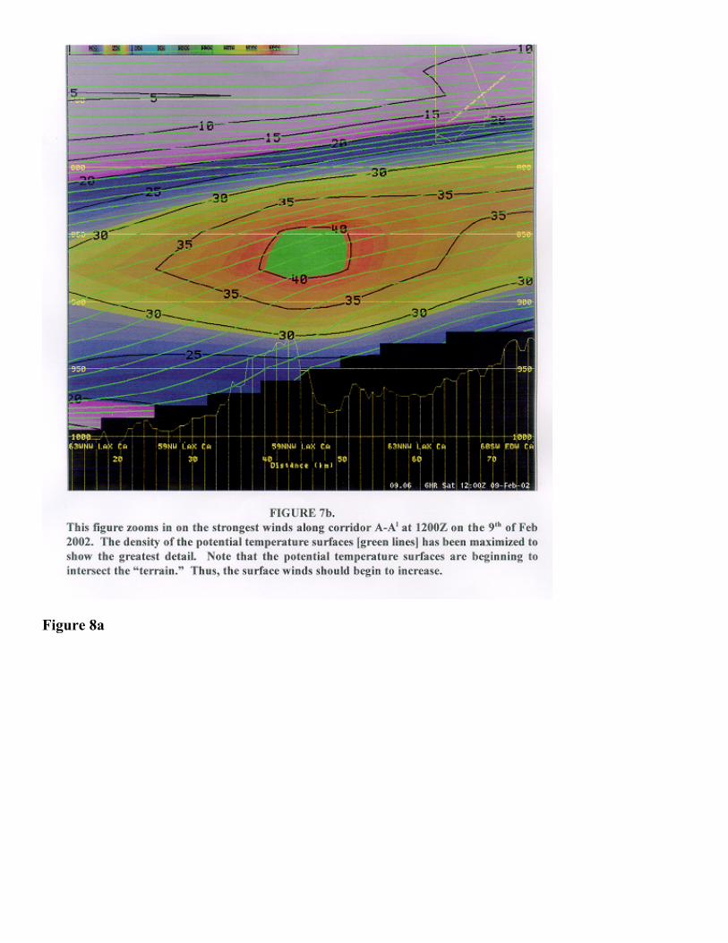
Figure 8a

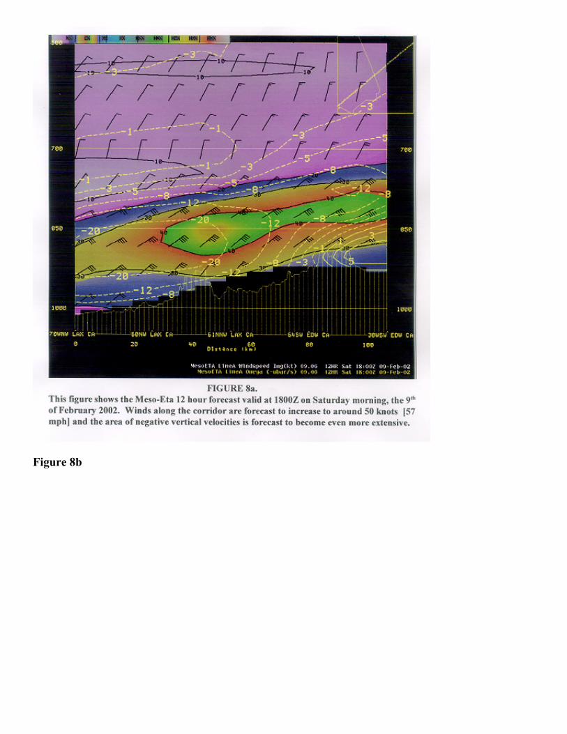
Figure 8b

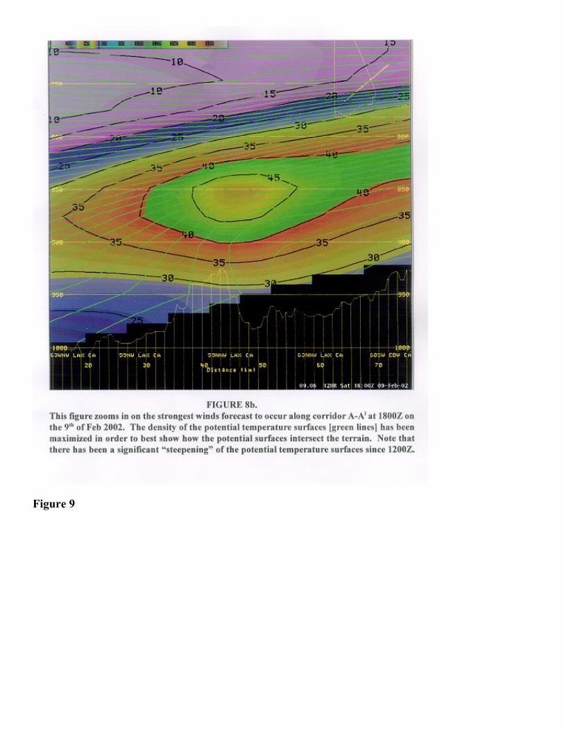
Figure 9

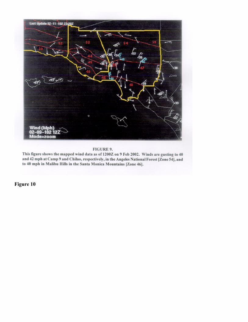
Figure 10