Space-time models with dust

and cosmological constant,

that allow integrating the

Hamilton-Jacobi test particle

equation by separation of

variables method.

Konstantin E. Osetrin

Tomsk State Pedagogical University

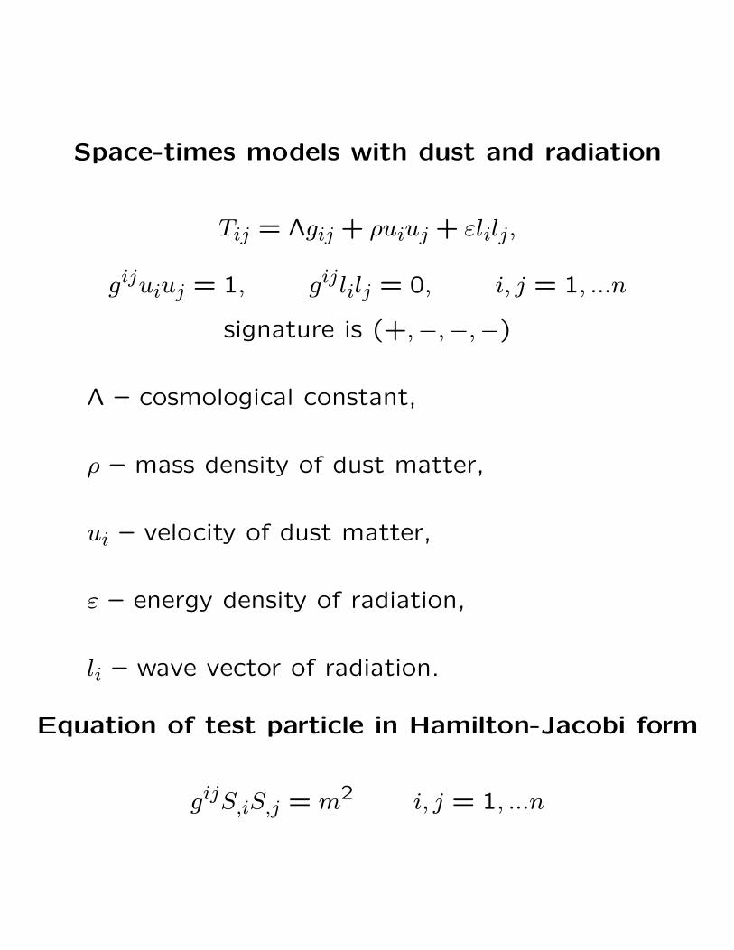
Space-times models with dust and radiation

Tij = Λgij + ρuiuj + εlilj,

gijuiuj = 1, gijlilj = 0, i, j = 1, ...n

signature is (+,−,−,−)

Λ – cosmological constant,

ρ – mass density of dust matter,

ui – velocity of dust matter,

ε – energy density of radiation,

li – wave vector of radiation.

Equation of test particle in Hamilton-Jacobi form

gijS,iS,j = m2 i, j = 1, ...n

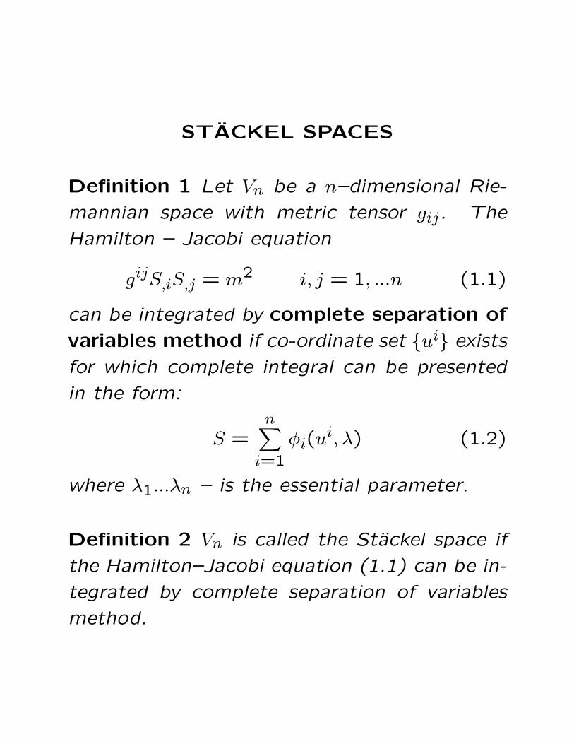
STACKEL SPACES

Definition 1 Let Vn be a n–dimensional Rie-

mannian space with metric tensor gij. The

Hamilton – Jacobi equation

gijS,iS,j = m2 i, j = 1, ...n (1.1)

can be integrated by complete separation of

variables method if co-ordinate set {ui} exists

for which complete integral can be presented

in the form:

S =n∑i=1

φi(ui, λ) (1.2)

where λ1...λn – is the essential parameter.

Definition 2 Vn is called the Stackel space if

the Hamilton–Jacobi equation (1.1) can be in-

tegrated by complete separation of variables

method.

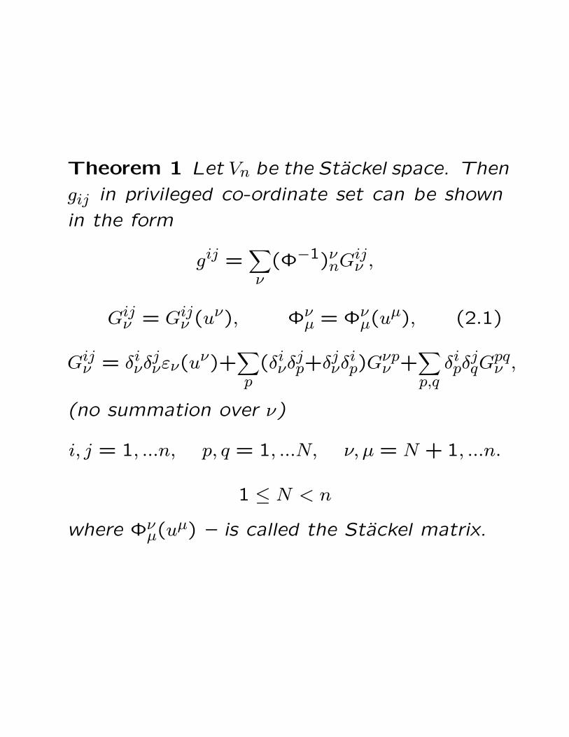
Theorem 1 Let Vn be the Stackel space. Then

gij in privileged co-ordinate set can be shown

in the form

gij =∑ν

(Φ−1)νnGijν ,

Gijν = Gijν (uν), Φνµ = Φν

µ(uµ), (2.1)

Gijν = δiνδjνεν(uν)+

∑p

(δiνδjp+δjνδ

ip)G

νpν +

∑p,qδipδ

jqG

pqν ,

(no summation over ν)

i, j = 1, ...n, p, q = 1, ...N, ν, µ = N + 1, ...n.

1 ≤ N < n

where Φνµ(uµ) – is called the Stackel matrix.

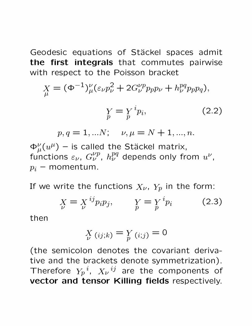
Geodesic equations of Stackel spaces admitthe first integrals that commutes pairwisewith respect to the Poisson bracket

Xµ

= (Φ−1)νµ(ενp2ν + 2Gνpν pppν + hpqν pppq),

Yp

= Ypipi, (2.2)

p, q = 1, ...N ; ν, µ = N + 1, ..., n.

Φνµ(uµ) – is called the Stackel matrix,

functions εν, Gνpν , hpqν depends only from uν,pi – momentum.

If we write the functions Xν, Yp in the form:

Xν

= Xνijpipj, Y

p= Y

pipi (2.3)

then

Xν (ij;k) = Y

p (i;j) = 0

(the semicolon denotes the covariant deriva-tive and the brackets denote symmetrization).Therefore Yp i, Xν ij are the components ofvector and tensor Killing fields respectively.

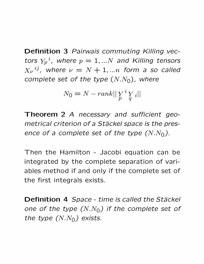
Definition 3 Pairwais commuting Killing vec-

tors Yp i, where p = 1, ...N and Killing tensors

Xν ij, where ν = N + 1, ...n form a so called

complete set of the type (N.N0), where

N0 = N − rank||YpiYq i||

Theorem 2 A necessary and sufficient geo-

metrical criterion of a Stackel space is the pres-

ence of a complete set of the type (N.N0).

Then the Hamilton - Jacobi equation can be

integrated by the complete separation of vari-

ables method if and only if the complete set of

the first integrals exists.

Definition 4 Space - time is called the Stackel

one of the type (N.N0) if the complete set of

the type (N.N0) exists.

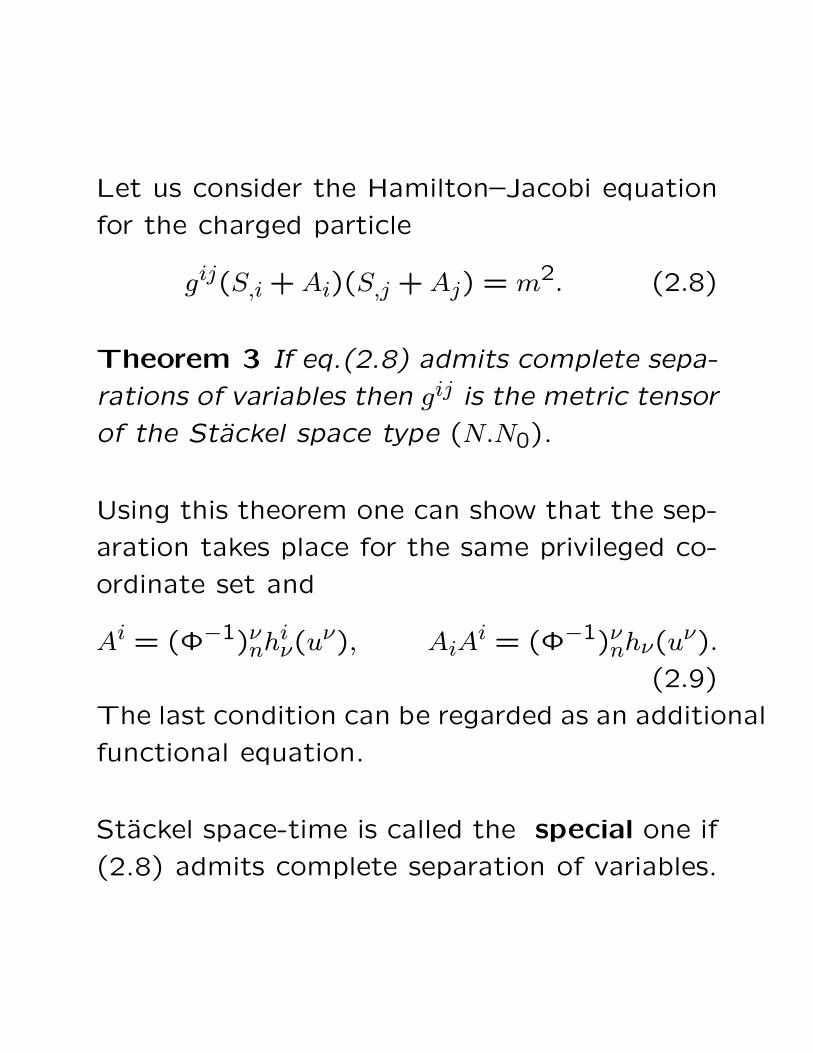
Let us consider the Hamilton–Jacobi equation

for the charged particle

gij(S,i +Ai)(S,j +Aj) = m2. (2.8)

Theorem 3 If eq.(2.8) admits complete sepa-

rations of variables then gij is the metric tensor

of the Stackel space type (N.N0).

Using this theorem one can show that the sep-

aration takes place for the same privileged co-

ordinate set and

Ai = (Φ−1)νnhiν(uν), AiA

i = (Φ−1)νnhν(uν).

(2.9)

The last condition can be regarded as an additional

functional equation.

Stackel space-time is called the special one if

(2.8) admits complete separation of variables.

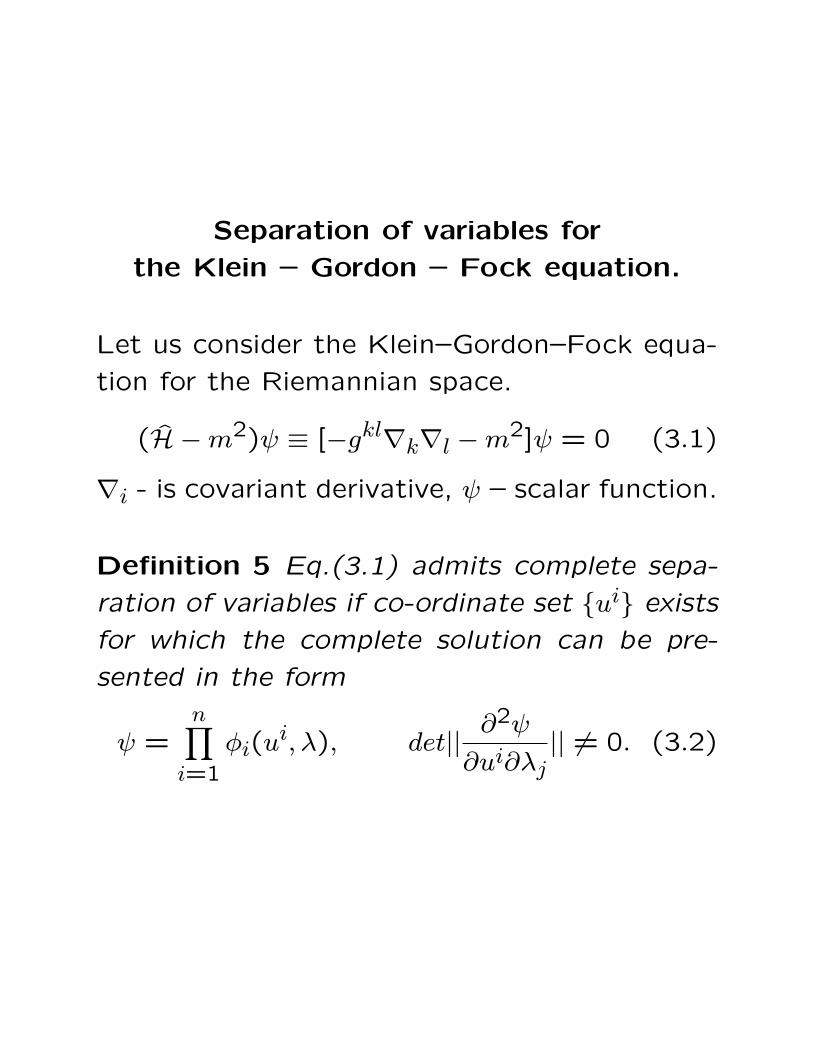
Separation of variables for

the Klein – Gordon – Fock equation.

Let us consider the Klein–Gordon–Fock equa-

tion for the Riemannian space.

(H −m2)ψ ≡ [−gkl∇k∇l −m2]ψ = 0 (3.1)

∇i - is covariant derivative, ψ – scalar function.

Definition 5 Eq.(3.1) admits complete sepa-

ration of variables if co-ordinate set {ui} exists

for which the complete solution can be pre-

sented in the form

ψ =n∏i=1

φi(ui, λ), det||

∂2ψ

∂ui∂λj|| 6= 0. (3.2)

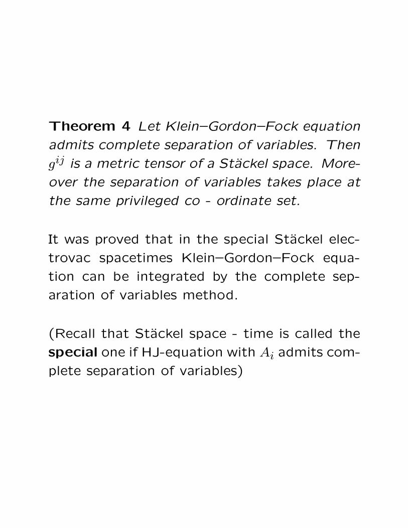
Theorem 4 Let Klein–Gordon–Fock equation

admits complete separation of variables. Then

gij is a metric tensor of a Stackel space. More-

over the separation of variables takes place at

the same privileged co - ordinate set.

It was proved that in the special Stackel elec-

trovac spacetimes Klein–Gordon–Fock equa-

tion can be integrated by the complete sep-

aration of variables method.

(Recall that Stackel space - time is called the

special one if HJ-equation with Ai admits com-

plete separation of variables)

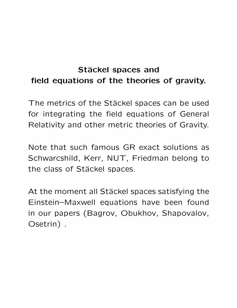
Stackel spaces and

field equations of the theories of gravity.

The metrics of the Stackel spaces can be used

for integrating the field equations of General

Relativity and other metric theories of Gravity.

Note that such famous GR exact solutions as

Schwarcshild, Kerr, NUT, Friedman belong to

the class of Stackel spaces.

At the moment all Stackel spaces satisfying the

Einstein–Maxwell equations have been found

in our papers (Bagrov, Obukhov, Shapovalov,

Osetrin) .

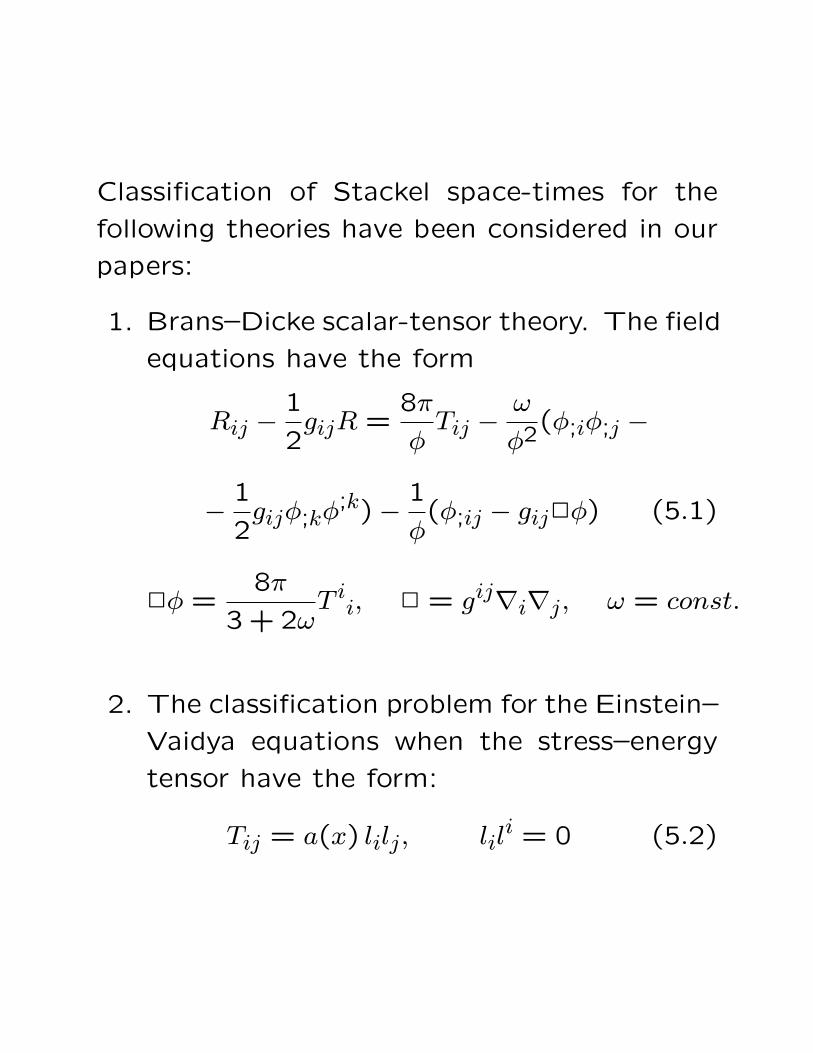
Classification of Stackel space-times for the

following theories have been considered in our

papers:

1. Brans–Dicke scalar-tensor theory. The field

equations have the form

Rij −1

2gijR =

8π

φTij −

ω

φ2(φ;iφ;j −

−1

2gijφ;kφ

;k)−1

φ(φ;ij − gij2φ) (5.1)

2φ =8π

3 + 2ωT ii, 2 = gij∇i∇j, ω = const.

2. The classification problem for the Einstein–

Vaidya equations when the stress–energy

tensor have the form:

Tij = a(x) lilj, lili = 0 (5.2)

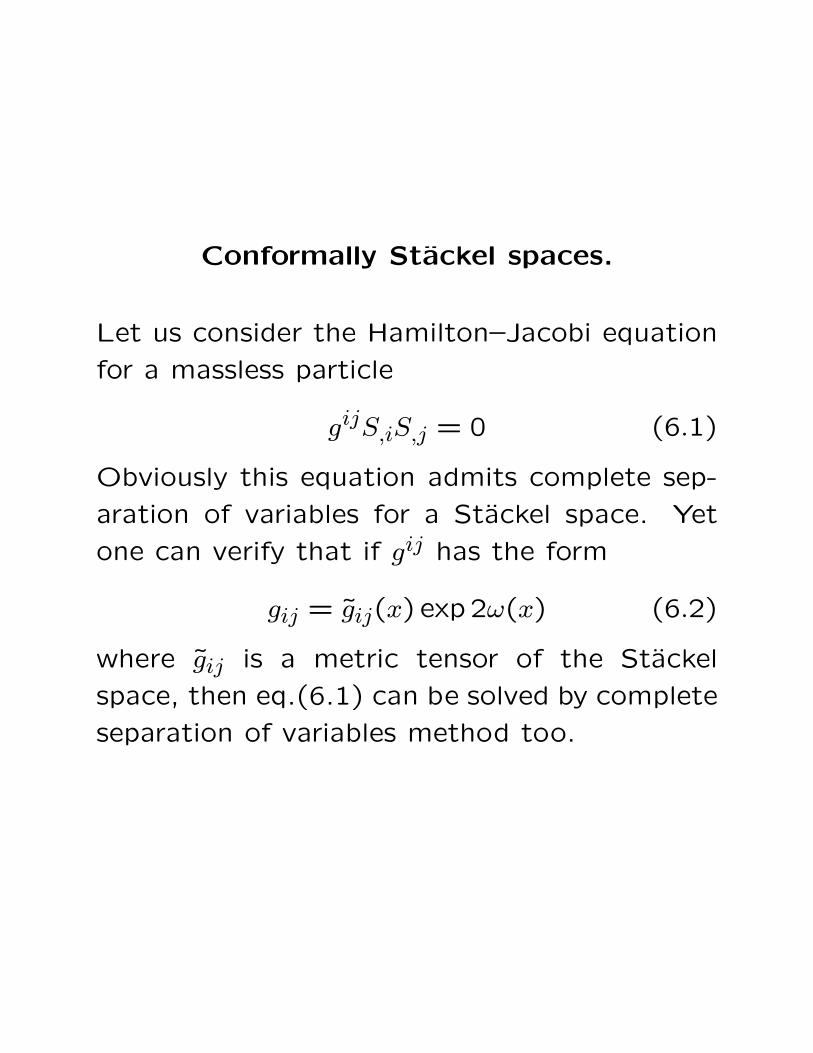
Conformally Stackel spaces.

Let us consider the Hamilton–Jacobi equation

for a massless particle

gijS,iS,j = 0 (6.1)

Obviously this equation admits complete sep-

aration of variables for a Stackel space. Yet

one can verify that if gij has the form

gij = gij(x) exp 2ω(x) (6.2)

where gij is a metric tensor of the Stackel

space, then eq.(6.1) can be solved by complete

separation of variables method too.

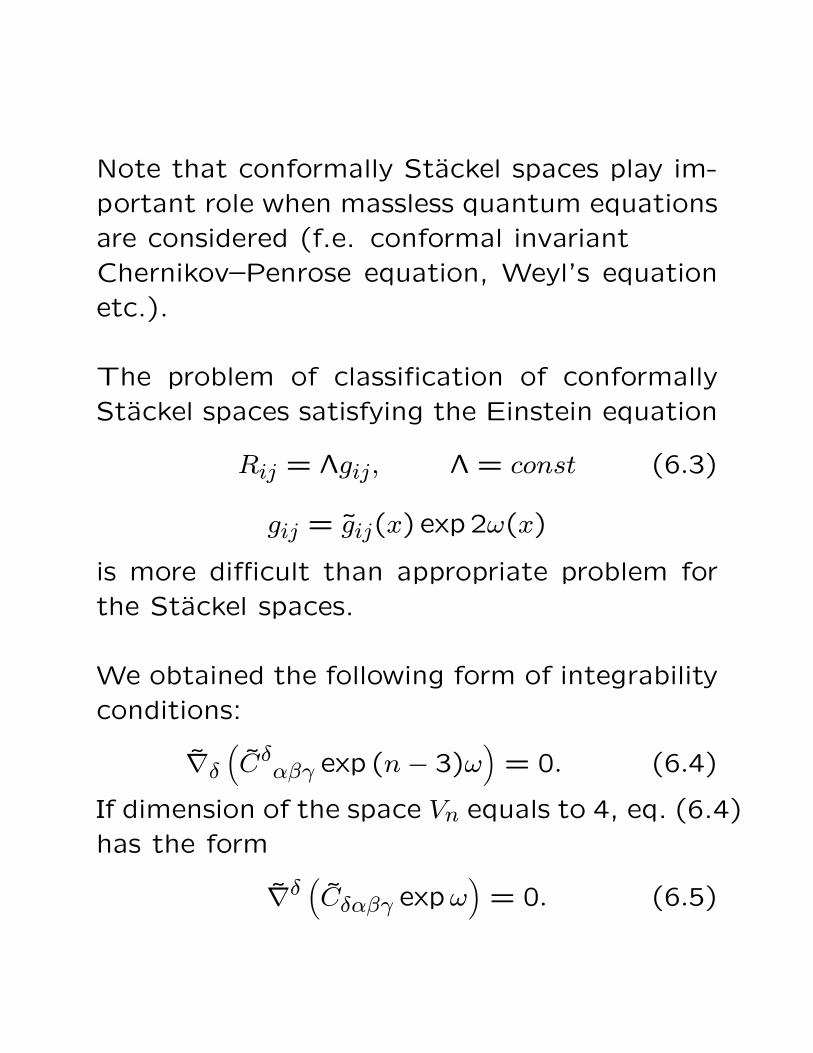
Note that conformally Stackel spaces play im-portant role when massless quantum equationsare considered (f.e. conformal invariantChernikov–Penrose equation, Weyl’s equationetc.).

The problem of classification of conformallyStackel spaces satisfying the Einstein equation

Rij = Λgij, Λ = const (6.3)

gij = gij(x) exp 2ω(x)

is more difficult than appropriate problem forthe Stackel spaces.

We obtained the following form of integrabilityconditions:

∇δ(Cδαβγ exp (n− 3)ω

)= 0. (6.4)

If dimension of the space Vn equals to 4, eq. (6.4)has the form

∇δ(Cδαβγ expω

)= 0. (6.5)

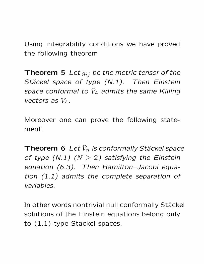
Using integrability conditions we have proved

the following theorem

Theorem 5 Let gij be the metric tensor of the

Stackel space of type (N.1). Then Einstein

space conformal to V4 admits the same Killing

vectors as V4.

Moreover one can prove the following state-

ment.

Theorem 6 Let Vn is conformally Stackel space

of type (N.1) (N ≥ 2) satisfying the Einstein

equation (6.3). Then Hamilton–Jacobi equa-

tion (1.1) admits the complete separation of

variables.

In other words nontrivial null conformally Stackel

solutions of the Einstein equations belong only

to (1.1)-type Stackel spaces.

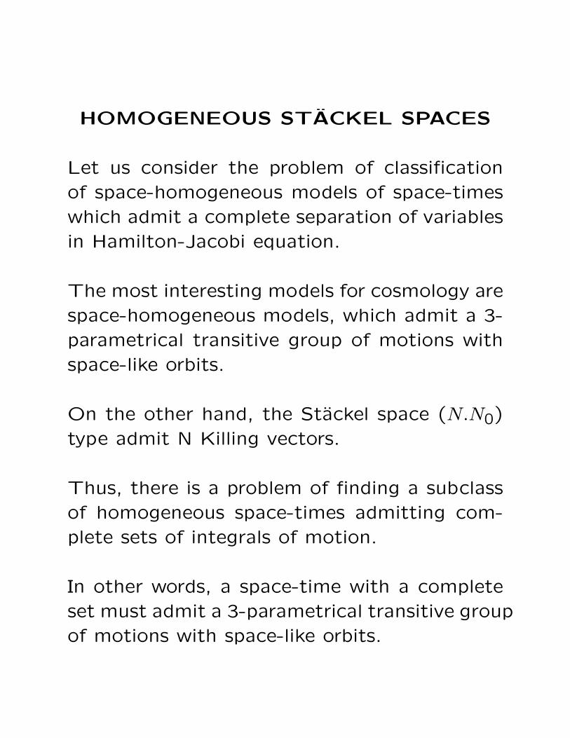
HOMOGENEOUS STACKEL SPACES

Let us consider the problem of classificationof space-homogeneous models of space-timeswhich admit a complete separation of variablesin Hamilton-Jacobi equation.

The most interesting models for cosmology arespace-homogeneous models, which admit a 3-parametrical transitive group of motions withspace-like orbits.

On the other hand, the Stackel space (N.N0)type admit N Killing vectors.

Thus, there is a problem of finding a subclassof homogeneous space-times admitting com-plete sets of integrals of motion.

In other words, a space-time with a completeset must admit a 3-parametrical transitive groupof motions with space-like orbits.

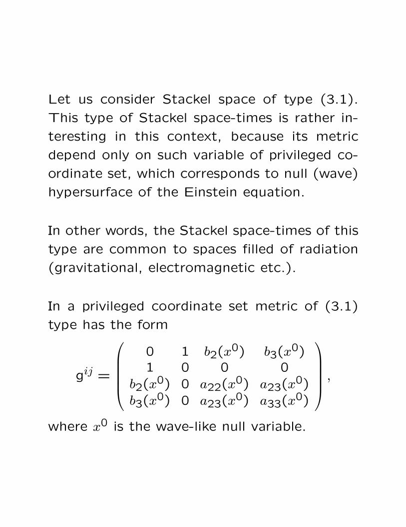
Let us consider Stackel space of type (3.1).

This type of Stackel space-times is rather in-

teresting in this context, because its metric

depend only on such variable of privileged co-

ordinate set, which corresponds to null (wave)

hypersurface of the Einstein equation.

In other words, the Stackel space-times of this

type are common to spaces filled of radiation

(gravitational, electromagnetic etc.).

In a privileged coordinate set metric of (3.1)

type has the form

gij =

0 1 b2(x0) b3(x0)1 0 0 0

b2(x0) 0 a22(x0) a23(x0)b3(x0) 0 a23(x0) a33(x0)

,where x0 is the wave-like null variable.

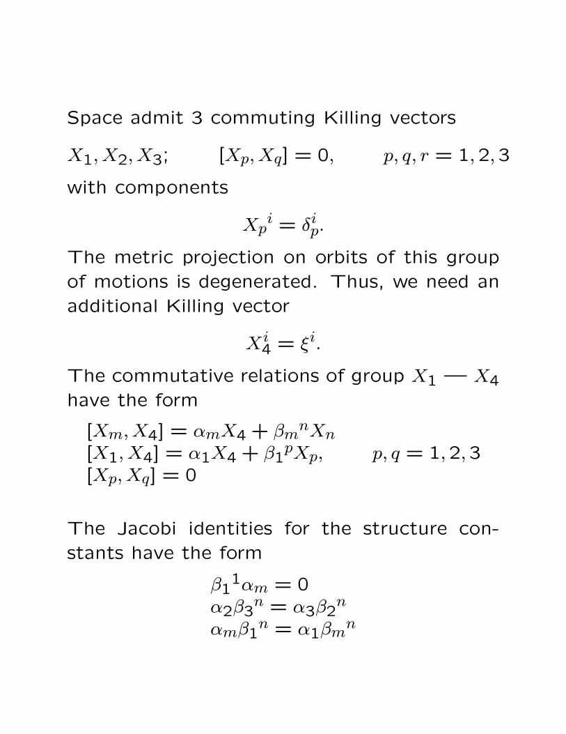
Space admit 3 commuting Killing vectors

X1, X2, X3; [Xp, Xq] = 0, p, q, r = 1,2,3

with components

Xpi = δip.

The metric projection on orbits of this groupof motions is degenerated. Thus, we need anadditional Killing vector

Xi4 = ξi.

The commutative relations of group X1 — X4

have the form

[Xm, X4] = αmX4 + βmnXn[X1, X4] = α1X4 + β1

pXp, p, q = 1,2,3[Xp, Xq] = 0

The Jacobi identities for the structure con-stants have the form

β11αm = 0

α2β3n = α3β2

n

αmβ1n = α1βm

n

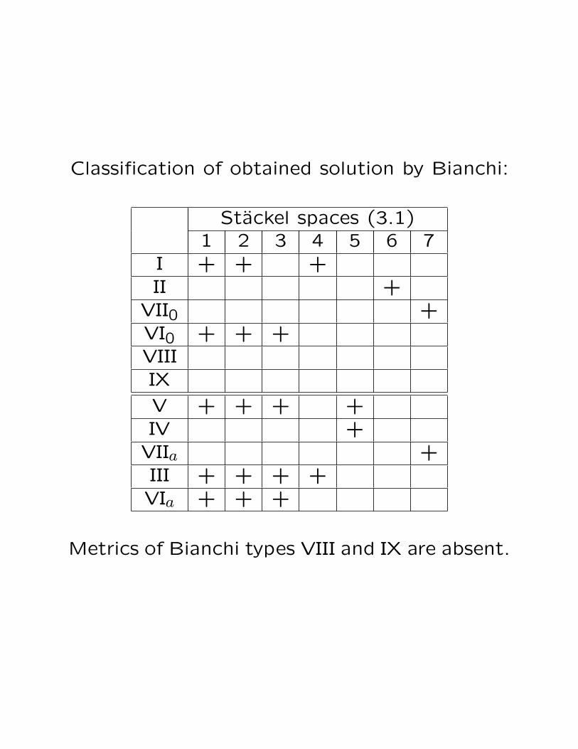
Classification of obtained solution by Bianchi:

Stackel spaces (3.1)1 2 3 4 5 6 7

I + + +II +

VII0 +VI0 + + +VIIIIX

V + + + +IV +

VIIa +III + + + +

VIa + + +

Metrics of Bianchi types VIII and IX are absent.

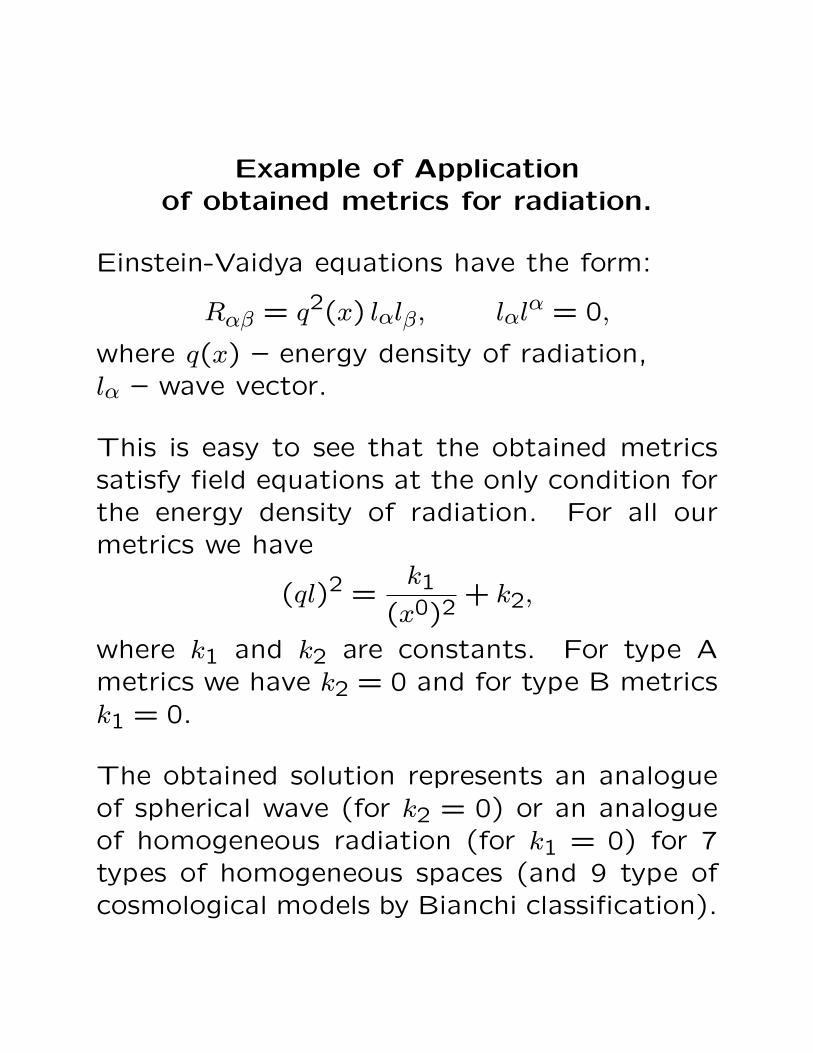
Example of Applicationof obtained metrics for radiation.

Einstein-Vaidya equations have the form:

Rαβ = q2(x) lαlβ, lαlα = 0,

where q(x) – energy density of radiation,lα – wave vector.

This is easy to see that the obtained metricssatisfy field equations at the only condition forthe energy density of radiation. For all ourmetrics we have

(ql)2 =k1

(x0)2+ k2,

where k1 and k2 are constants. For type Ametrics we have k2 = 0 and for type B metricsk1 = 0.

The obtained solution represents an analogueof spherical wave (for k2 = 0) or an analogueof homogeneous radiation (for k1 = 0) for 7types of homogeneous spaces (and 9 type ofcosmological models by Bianchi classification).

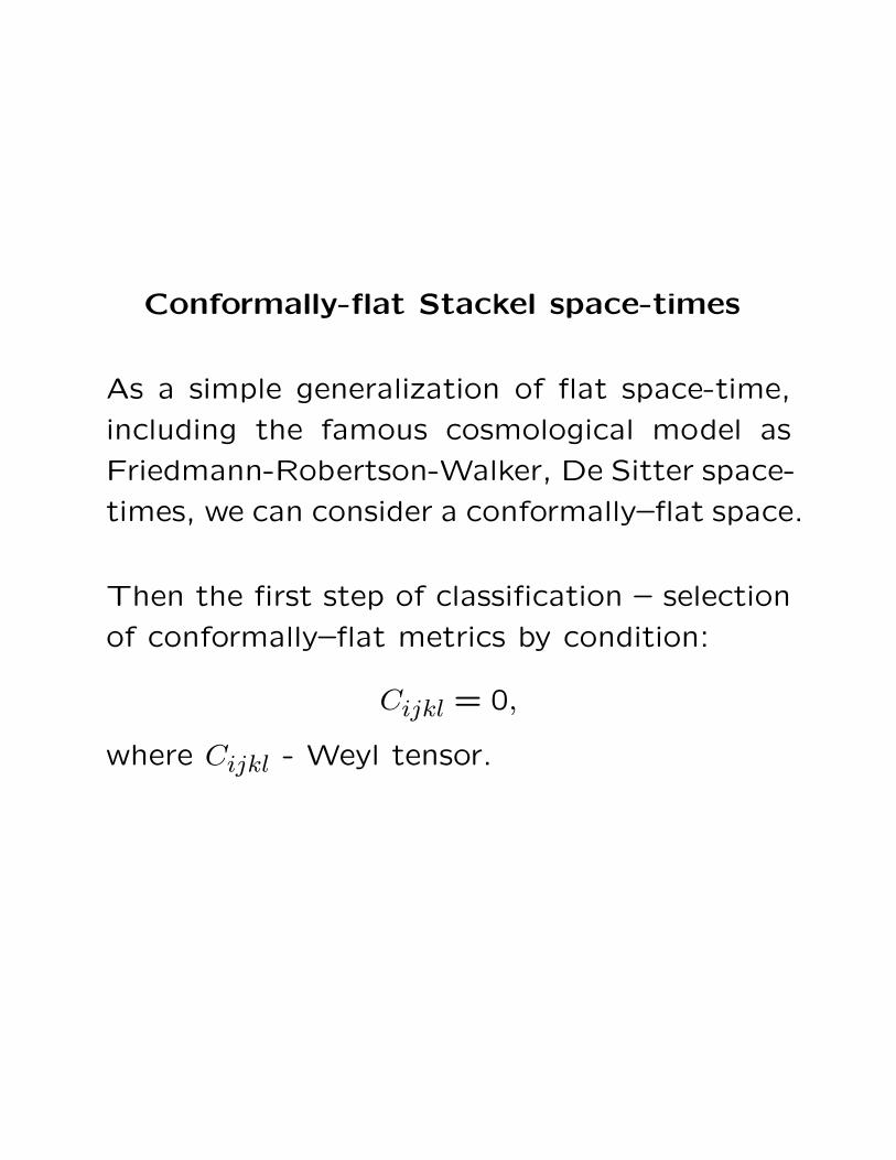
Conformally-flat Stackel space-times

As a simple generalization of flat space-time,

including the famous cosmological model as

Friedmann-Robertson-Walker, De Sitter space-

times, we can consider a conformally–flat space.

Then the first step of classification – selection

of conformally–flat metrics by condition:

Cijkl = 0,

where Cijkl - Weyl tensor.

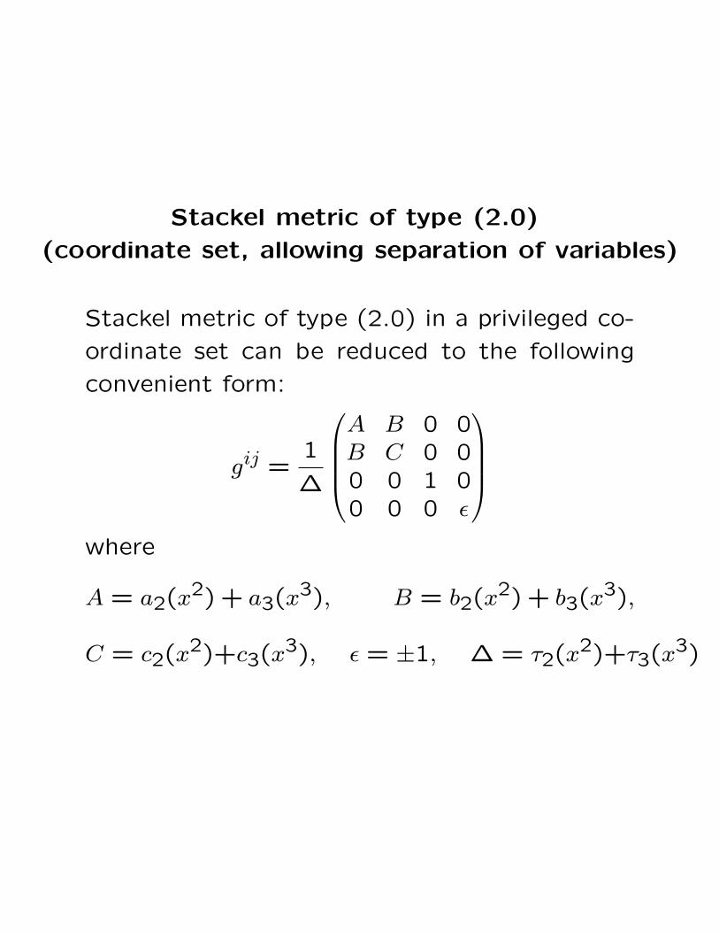
Stackel metric of type (2.0)

(coordinate set, allowing separation of variables)

Stackel metric of type (2.0) in a privileged co-

ordinate set can be reduced to the following

convenient form:

gij =1

∆

A B 0 0B C 0 00 0 1 00 0 0 ε

where

A = a2(x2) + a3(x3), B = b2(x2) + b3(x3),

C = c2(x2)+c3(x3), ε = ±1, ∆ = τ2(x2)+τ3(x3)

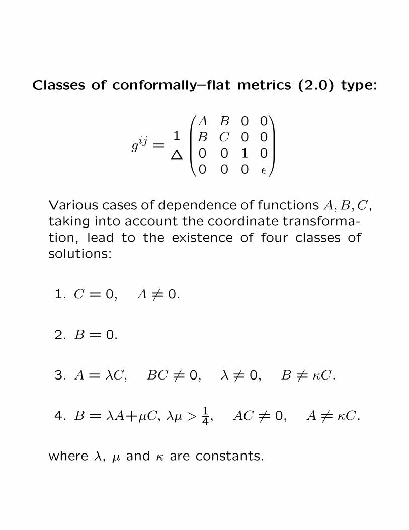
Classes of conformally–flat metrics (2.0) type:

gij =1

∆

A B 0 0B C 0 00 0 1 00 0 0 ε

Various cases of dependence of functions A,B,C,taking into account the coordinate transforma-tion, lead to the existence of four classes ofsolutions:

1. C = 0, A 6= 0.

2. B = 0.

3. A = λC, BC 6= 0, λ 6= 0, B 6= κC.

4. B = λA+µC, λµ > 14, AC 6= 0, A 6= κC.

where λ, µ and κ are constants.

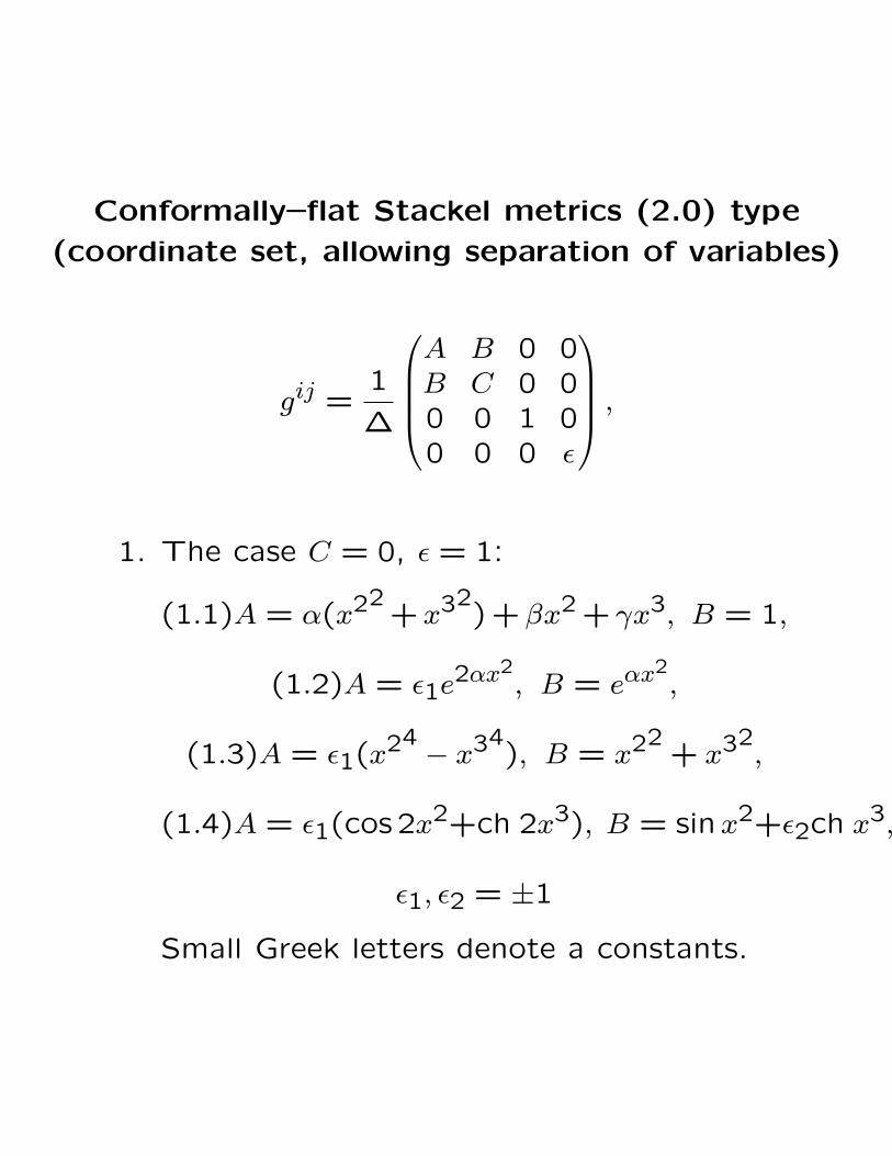
Conformally–flat Stackel metrics (2.0) type

(coordinate set, allowing separation of variables)

gij =1

∆

A B 0 0B C 0 00 0 1 00 0 0 ε

,

1. The case C = 0, ε = 1:

(1.1)A = α(x22+ x32

) + βx2 + γx3, B = 1,

(1.2)A = ε1e2αx2

, B = eαx2,

(1.3)A = ε1(x24 − x34), B = x22

+ x32,

(1.4)A = ε1(cos 2x2+ch 2x3), B = sinx2+ε2ch x3,

ε1, ε2 = ±1

Small Greek letters denote a constants.

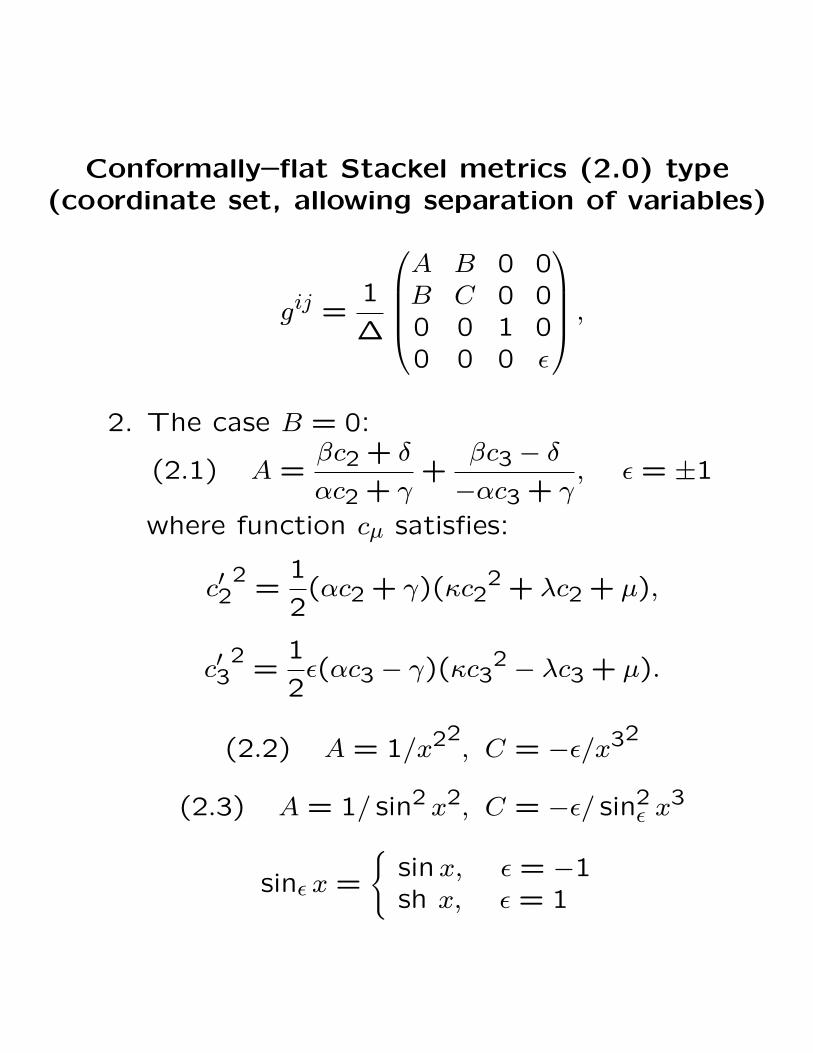
Conformally–flat Stackel metrics (2.0) type(coordinate set, allowing separation of variables)

gij =1

∆

A B 0 0B C 0 00 0 1 00 0 0 ε

,

2. The case B = 0:

(2.1) A =βc2 + δ

αc2 + γ+

βc3 − δ−αc3 + γ

, ε = ±1

where function cµ satisfies:

c′22

=1

2(αc2 + γ)(κc2

2 + λc2 + µ),

c′32

=1

2ε(αc3 − γ)(κc3

2 − λc3 + µ).

(2.2) A = 1/x22, C = −ε/x32

(2.3) A = 1/ sin2 x2, C = −ε/ sin2ε x

3

sinε x =

{sinx, ε = −1sh x, ε = 1

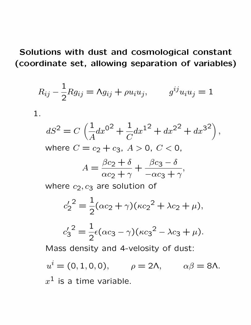
Solutions with dust and cosmological constant

(coordinate set, allowing separation of variables)

Rij −1

2Rgij = Λgij + ρuiuj, gijuiuj = 1

1.

dS2 = C

(1

Adx02

+1

Cdx12

+ dx22+ dx32

),

where C = c2 + c3, A > 0, C < 0,

A =βc2 + δ

αc2 + γ+

βc3 − δ−αc3 + γ

,

where c2, c3 are solution of

c′22

=1

2(αc2 + γ)(κc2

2 + λc2 + µ),

c′32

=1

2ε(αc3 − γ)(κc3

2 − λc3 + µ).

Mass density and 4-velosity of dust:

ui = (0,1,0,0), ρ = 2Λ, αβ = 8Λ.

x1 is a time variable.

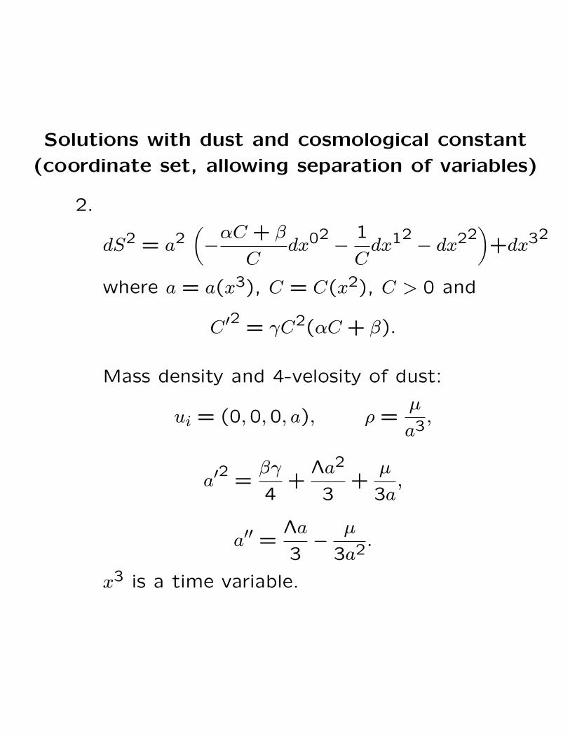
Solutions with dust and cosmological constant

(coordinate set, allowing separation of variables)

2.

dS2 = a2(−αC + β

Cdx02 −

1

Cdx12 − dx22

)+dx32

where a = a(x3), C = C(x2), C > 0 and

C′2 = γC2(αC + β).

Mass density and 4-velosity of dust:

ui = (0,0,0, a), ρ =µ

a3,

a′2 =βγ

4+

Λa2

3+

µ

3a,

a′′ =Λa

3−

µ

3a2.

x3 is a time variable.

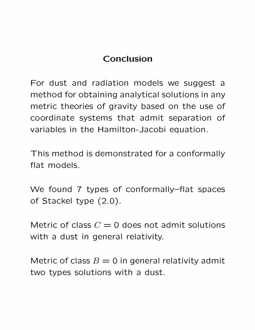
Conclusion

For dust and radiation models we suggest a

method for obtaining analytical solutions in any

metric theories of gravity based on the use of

coordinate systems that admit separation of

variables in the Hamilton-Jacobi equation.

This method is demonstrated for a conformally

flat models.

We found 7 types of conformally–flat spaces

of Stackel type (2.0).

Metric of class C = 0 does not admit solutions

with a dust in general relativity.

Metric of class B = 0 in general relativity admit

two types solutions with a dust.