Spectral Elements for Two-dimensional Resistive MHDhientzsc/matlab.pdf · 2005-04-15 · Spectral Elements for Two-dimensional Resistive MHD ... (s) and time ... are a standard Laplace

Spectral Elements for Two-dimensional

Resistive MHD

Bernhard HientzschCourant Institute of Mathematical Sciences

New York Universitymailto:[email protected]

http://www.math.nyu.edu/~hientzsc

April 15, 2005

Technical Presentation at The MathWorksApril 15, 2005

Natick, Massachusetts

Bernhard Hientzsch SEM for 2D resistive MHD

Overview of the Technical Presentation

• Description of the project

• My approach

• Formulation, discretization, and problem considered

• Implementation in C/LAPACK/BLAS

MathWorks Technical Presentation 04/15/2005 1


Description of the project

• M3D implements a particular formulation of magnetohydrodynamics(MHD), discretized using both finite differences and finite elements.Written by a team mostly at Princeton Plasma Physics Laboratory, butalso one team member from New York University (Hank Strauss).

• M3D used to simulate plasmas in fusion experiments and possible futurefusion reactors. Many extensions of MHD: two fluid models, particles,etc.

• Goal: study of linearly unstable modes (or almost unstable modes) andtheir nonlinear evolution (saturation, blow-up, or ...). In stable fusionexperiment or successfull fusion reactor, all unstable modes must becontrolled or suppressed.

• There are many instabilities or modes that are studied: tilting modes,tearing modes, kink modes, fishbones, balooning modes, ELMs ...



Description of the project, II

• The formulation(s) and time discretization is given and fixed (or coding itshould require only small changes), but there were/are different versionswith different space discretizations. All of them until now lower order,mostly even just linear elements.

• My project is to test spectral elements (SEM) as a space discretizationfor this formulation on some examples; validate them as an approach onsome examples; and propose algorithms and write modules for inclusionin M3D.

• Also, I am acting as somewhat of a consultant for some issues in finiteelements/numerical analysis/scientific computing for the group. Someof my suggestions have made their way into the code ...



My approach

• Have codes for SEM for other problems. (Linear and nonlinear ellipticequations and Maxwell equations.) Use as basis for coding.

• Rapid prototype discretizations and methods. Chose simple andstraightforward approaches to get into the problem as fast as possible.Try on structured grids and easy domains first to be able to use fastsolvers.

• Rapid prototype the programming. MATLAB/PYTHON 7→C/LAPACK/BLAS 7→ PETSc 7→ M3D.

• Fast solver: quick turnaround and extensive testing possible in MATLAB.Implement promising methods in C/LAPACK/BLAS. Validate and debugthem using MATLAB codes. Validate and debug more general solvers(for instance for isoparametric mapped elements) on the easy domains.



Formulation, discretization, and problem considered

• Incompressible resistive MHD in 2D: primitive variables, potentials.

• Time discretization (Finite Differences), timestepping algorithm.

• Space discretization (Spectral elements): short introduction,discretization of terms, fast solvers.

• Numerical examples: Tilting mode problem: Setup of problem, numericalresults: variables, energies, peak currents, growth rates.



Incompressible resistive MHD: primitive variables

∇u is the gradient: ∇u :=(

∂u∂x, ∂u

∂y

)

∇2u is the Laplacian: ∇2u := ∂2u∂x2 + ∂2u

∂y2

B: magnetic field, v: velocity field.ρ: density, here assumed constant. µ: viscosity. η: resistivity.

∂B

∂t= curl(v ×B) + η∇2B

ρ∂v

∂t= −ρv · ∇v + curlB ×B + ρµ∇2v

div v = 0

divB = 0



Incompressible resistive MHD: potential form in 2D

(vorticity-magnetic flux, Poisson brackets)

v = curlφ with velocity flux φ. B = curlψ with magnetic flux ψ.Ω: vorticity. C: current density.

Poisson bracket [a, b] := ∂a∂x

∂b∂y

− ∂b∂x

∂a∂y

.

∂Ω

∂t= [C,ψ] − [Ω, φ] + µ∇2Ω

∂ψ

∂t= −[ψ, φ] + η∇2ψ

∇2φ = Ω

C = ∇2ψ



Time discretization (semi-implicit)

Semi-implicit: diffusive terms implicit, all others explicit. Straightforwardfirst-order time-stepping. Arrange the equations and solve them one afterthe other. Leads to leapfrog method, using most recent values for variables.

Ωn+1 − Ωn

∆t= [Cn, ψn] − [Ωn, φn] + µ∇2Ωn+1

∇2φn+1 = Ωn+1

ψn+1 − ψn

∆t= −[ψn, φn+1] + η∇2ψn+1

Cn+1 = ∇2ψn+1



PDEs to be solved in each time-step

Ωn+1 − µ∆t∇2Ωn+1 = Ωn + ∆t [Cn, ψn] − [Ωn, φn] (1)

∇2φn+1 = Ωn+1 (2)

ψn+1 − η∆t∇2ψn+1 = ψn − ∆t[ψn, φn+1] (3)

Cn+1 = ∇2ψn+1 (4)

(1) and (3) are Helmholtz solves, for (I + α∇2) with α = −µ∆t andα = −η∆t, respectively. For mu = 0 or η = 0, respectively, these solvessimplify to direct assignments (PDE formulation) or L2-projections (weakformulation) taking into account the given boundary conditions. (2) and(4) are a standard Laplace solve respective application of the Laplacian.



Time stepping algorithm

A time-stepping algorithm can be implemented like (with P (a, b) a givendiscretization/approximation of [a, b]):

Ωn+1 = HHSolve(−µ∆t,Ωn + ∆tP (Cn, ψn) − ∆tP (Ωn, φn))

φn+1 = LapSolve(Ωn+1)

ψn+1 = HHSolve(−η∆t, ψn − ∆tP (ψn, φn+1))

Cn+1 = ApplyLap(ψn+1)

Some optimization possible in computation of right hand side by savingterms occuring at several places. Right hand side assembly only need modulefor Poisson bracket P if modularity is more important. Different boundary orcontinuity conditions or different degrees of freedom only change HHSolve,LapSolve, and ApplyLap; the code can reuse the same frame.



Time-stepping code fragment in MATLAB

omexrhs=pbrh(c,psi,disc)+pbrh(phi,omega,disc)+soOm;

omrhs=omega+dt*omexrhs;

omega=SolveHH(omrhs,disc,hhdisco);

phi=SolveSLap(omega,disc);

psrhs=dt*(pbrh(phi,psi,disc)+soPs-eta*ApplyLap0Bc(psi,disc));

dpsi=SolveHH(psrhs,disc,hhdiscp);

psi=psi+dpsi;

c=ApplySLap0Bc(psi,disc);

Intermediate results are put into variables because of other optionsand algorithmic possibilities not shown here. pbrh is a function handle.disc is a context structure for the discretization containing one-dimensionalmatrices etc. hhdisco and hhdiscp are context structures for the fastHelmholtz solves. All solves assume zero Dirichlet data. BCs from tiltingmode problem.



Why spectral elements?

• Exponential convergence for (standard) problems with (piecewise)smooth solutions. Alighnment, postprocessing, filtering etc. for otherproblems and solutions might restore exponential convergence.

• Fast application of stiffness and mass matrix. Fast solvers for rectangularelements and rectangles. Helmholtz there: generalized Sylvesterequation.

• Relatively straight-forward implementation. Expressed in matrix-matrixmultiplications, element-wise multiplications, and a few other matrixand vector operations. Translates into matrix-heavy MATLAB orC/C++/FORTRAN using LAPACK/BLAS.

• Can run at high percentages of peak on modern computer architectures:sparse block matrix with dense blocks. Paul Fischer won Gordon BellPrize with spectral element methods for Navier-Stokes equations.



Spectral elements, Introduction

• Approximate function in elements by high-order polynomials from tensorproduct space. Parametrize by values on (mapped) GLL grid.

• Differentiation, interpolation between grids, exact and approximateintegrals of products 7→ matrices acting on values on grid.

• On multi-dimensional non-distorted rectangular elements, matrices aretensor products matrices. F.i., x-derivative in 2D in element aligned withaxes is (D ⊗ I): derivative only acts along one coordinate.

• Bilinearly or isoparametrically mapped elements: operators are productsof block tensor product matrices and diagonal matrices.

• (A⊗B)u can be rewritten as matrix-matrix multiplication AUBT , whereU and result are 2D arrays instead of vectors.



Spectral elements, Helmholtz

• PDE: u + α∇2u = f , integrate by parts to obtain weak form: ∀v ∈H1

0 find u ∈ H10 satisfying (u, v) − α(∇u,∇v) = (u, v) − α(ux, vx) −

α(uy, vy) = (f, v).

• Instead of H10 , use polynomial space and matrices: vTMu −

αvTDTxMDxu− αvTDT

y MDyu = vTMf .

• (Mx⊗My)u−α(Dx,T ⊗ I)(Mx⊗My)(Dx⊗ I)u−α(I⊗Dy,T )(Mx⊗My)(I ⊗Dy)u = (Mx ⊗My)f

• (Mx ⊗My − αKx ⊗My − αMx ⊗Ky)u = (Mx ⊗My)f

• ((12M

x − αKx) ⊗My +Mx ⊗ (12M

y − αKy))u = (Mx ⊗My)f

• (Ax ⊗My +Mx ⊗ Ay)u = (Mx ⊗My)f or AxUMy,T +MxUAy,t =MxFMy,T (Generalized Sylvester equation.)



Spectral elements, Fast Solvers

Several methods to solve generalized Sylvester equations:

• Solve two generalized eigenvalue problems and diagonalize system bywriting in eigenbasis (fast diagonalization method).

• Transform matrix pairs to Schur form, and the transformed system(triangular in a sense) is solvable by back-substitution.

• Transform matrix pair to Schur/Hessenberg form, and then solvetriangular and Hessenberg systems.

First choice seems to be fast and stable enough for our computations.Second and third choice should be more stable, have implementation ofsecond choice. Do not see much difference in numerical behavior.



Spectral elements, Poisson Brackets

Need to approximate ([a, b], c) =(

∂a∂x

∂b∂y

− ∂a∂y

∂b∂x, v

)

Approximate inner product by mass matrix M as before. Compute anapproximation to [a, b] on some GLL grid by possible interpolation and thenpointwise multiplication ⊛:

([a, b], v) ≈ vTM((Dxa) ⊛ (Dyb) − (Dya) ⊛ (Dxb) =: vTMP (a, b)

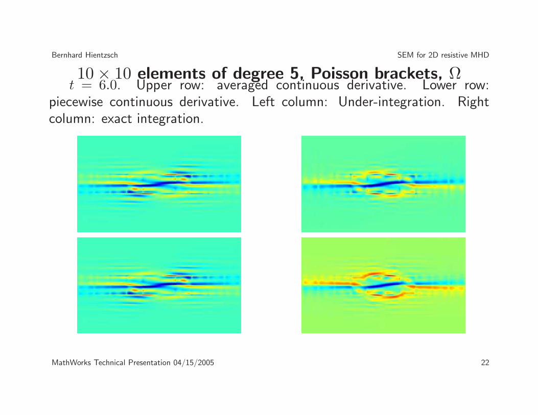
Now one can choose on which grid one wants to evaluate [a, b] (on theoriginal grid this would lead to under-integration, on a grid of high enoughdegree exact integration) and if one treats the result as piecewise continuousas straighforward differentiation would give, or one could use an averagedor projected version that is globally continuous.



Tilting mode problem - Setup

Introduce polar coordinates x = r cosφ, y = r sinφ, and use separableform in polar coordinates,

ψ(t = 0) = ψ0,rad(r) cos θ Ω(t = 0) = ǫΩ0,pert(r)

with the radial functions (k being the first positive zero of J1, k ≈ 3.8317):

ψ0,rad(r) =

2J1(kr)kJ0(k) for r ≤ 1r2−1r

for r ≥ 1Ω0,pert(r) = 4(r2−1) exp(−r2)

The following boundary conditions were use in this problem:

φ = 0 C = 0∂ψ

∂t= 0 Ω = 0



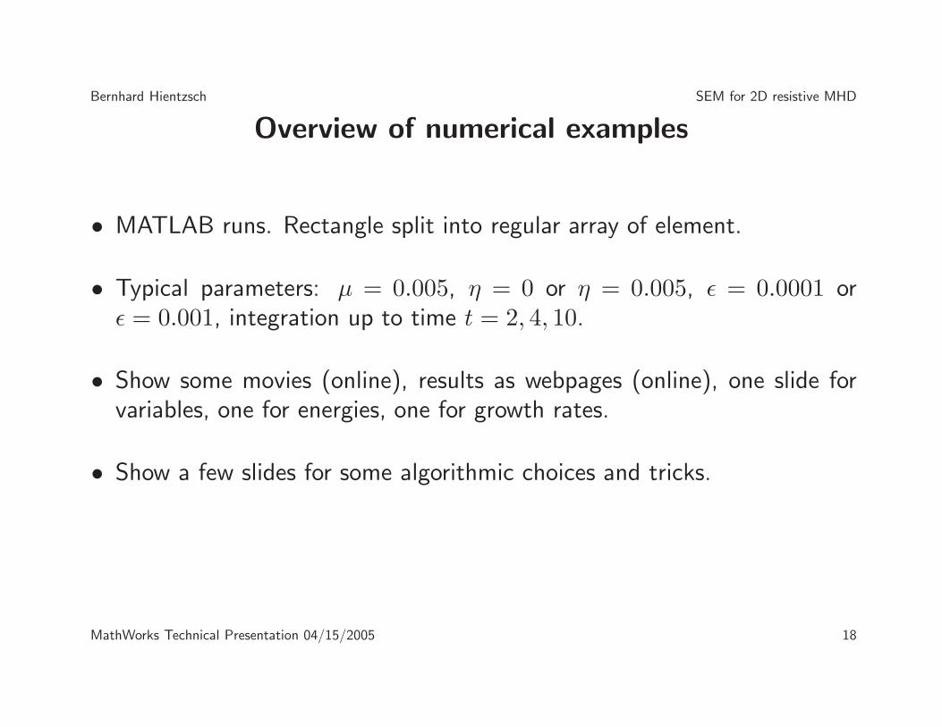
Overview of numerical examples

• MATLAB runs. Rectangle split into regular array of element.

• Typical parameters: µ = 0.005, η = 0 or η = 0.005, ǫ = 0.0001 orǫ = 0.001, integration up to time t = 2, 4, 10.

• Show some movies (online), results as webpages (online), one slide forvariables, one for energies, one for growth rates.

• Show a few slides for some algorithmic choices and tricks.



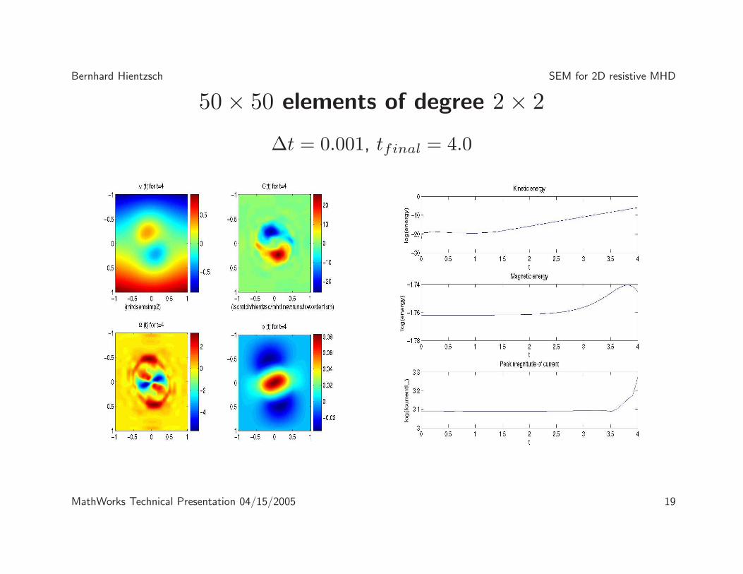
50 × 50 elements of degree 2 × 2

∆t = 0.001, tfinal = 4.0



5 × 5 elements: Kinetic Energies

Upper left: degree 5 × 5, upper right: degree 6 × 6, lower left: degree10 × 10, lower right: degree 20 × 20.

-20

-15

-10

-5

0 0.5 1 1.5 2 2.5 3 3.5 4

kine

tic e

nerg

y

x

kinetic energy (data from 5x5deg5.enercur.dat)

log(kinetic energy)

-20

-15

-10

-5

0 0.5 1 1.5 2 2.5 3 3.5 4

kine

tic e

nerg

y

x


log(kinetic energy)

-20

-15

-10

-5

0 0.5 1 1.5 2 2.5 3 3.5 4

kine

tic e

nerg

y

x


log(kinetic energy)

-20

-15

-10

-5

0 0.5 1 1.5 2 2.5 3 3.5 4

kine

tic e

nerg

y

x


log(kinetic energy)



5 × 5 elements: Growth rates• As seen on the last slide, the kinetic energy grows exponentially.

• Since the computation there did not include resistivity, the growthactually never stops and the mode never saturates nonlinearly.

• Initial stages show how the initial pertubation slowly shifts energy tothe unstable mode, and after some time the exponential growth of thatlinearly unstable mode overshadows the results.

• One important characteristic of an unstable mode is its growth rate,which is the coefficient of the exponential growth. Eyeballing the domainof exponential growth and fitting an exponential, the following growthrate were observed: 5 - 1.2065, 6 - 1.2543, 10 - 1.2398, 20 - 1.2417.The consensus estimates in the field are 1.23-1.25, so that our growthrates are in the ballpark. Computations seem to be reasonable to plasmaphysicists inspecting them.



10 × 10 elements of degree 5, Poisson brackets, Ωt = 6.0. Upper row: averaged continuous derivative. Lower row:

piecewise continuous derivative. Left column: Under-integration. Rightcolumn: exact integration.



10 × 10 elements of degree 5, Poisson brackets, C



10 × 10 elements of degree 5, C1 filtering



Implementation in C

• Simple idea: code all the matrix operations and algorithms that arealready written in high-level linear algebra form in my MATLAB codenow in C using LAPACK and BLAS.

• Figuring out compilation and optimization for vendor-specific highperformance libraries is ”interesting”. MATLAB does a lot of things (likeeigenvalue computations and other matrix operations) very efficientlyand makes many choices for the uses, while a lot of those hidden detailhave to be coded explicitly when using LAPACK/BLAS /ATLAS directly.

• By now, there is a reasonable code base for SUN and for Linux Pentium.(The later is complete only on a now dead laptop in its latest form,back-up is a little bit more than a week old and is not as advanced.) Askeleton version of the entire package was running, but visualization andmore extensive runs are not yet done.



Implementation in C: maximum error

0 50 100 150 200−14

−12

−10

−8

−6

−4

−2

0

2

N − element is degree NxN

log

10(|

ma

x−e

rro

r|)

Maximum errors for Dirichlet problem for Laplace equation (Transformation to Eigenbasis)

MATLAB on SunC/SUNPERFLIB on Sun



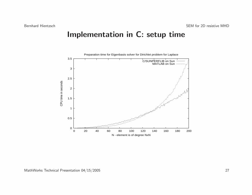
Implementation in C: setup time

0

0.5

1

1.5

2

2.5

3

3.5

0 20 40 60 80 100 120 140 160 180 200

CP

U ti

me

in s

econ

ds

N - element is of degree NxN

Preparation time for Eigenbasis solver for Dirichlet problem for Laplace

C/SUNPERFLIB on SunMATLAB on Sun



Implementation in C: time for actual solve

0

0.5

1

1.5

2

2.5

3

0 20 40 60 80 100 120 140 160 180 200

CP

U ti

me

in s

econ

ds

N - element is of degree NxN

Solve time for Eigenbasis solver for Dirichlet problem for Laplace

C/Sunperflib on SunMATLAB on Sun



Results from my (dead) laptop - IBM Thinkpad T30

1e-16

1e-14

1e-12

1e-10

1e-08

1e-06

1e-04

0.01

1

0 50 100 150 200 250 300 350 400

log 1

0(|m

ax-e

rror

|)

n (element is degree nxn)

gsylvevprep/gsylvevsolv(C/LAPACK/ATLAS): Dirichlet problem for Laplace (Laptop)

Maximum error



0

0.5

1

1.5

2

2.5

3

0 50 100 150 200 250 300 350 400

CP

U ti

me

in s

econ

ds



Preparing the solve



0

0.05

0.1

0.15

0.2

0.25

0.3

0.35

0.4

0 50 100 150 200 250 300 350 400

CP

U ti

me

in s

econ

ds



Actual solve


Documents

Spectral Elements for Two-dimensional Resistive MHDhientzsc/matlab.pdf · 2005-04-15 · Spectral Elements for Two-dimensional Resistive MHD ... (s) and time ... are a standard Laplace