FL47CH19-Clanet ARI 18 November 2014 13:26

Sports BallisticsChristophe ClanetLadHyX, UMR7646, CNRS, Ecole Polytechnique, 91128 Palaiseau, France;email: christophe.clanet@ladhyx.polytechnique.fr

Annu. Rev. Fluid Mech. 2015. 47:455–78

First published online as a Review in Advance onSeptember 22, 2014

The Annual Review of Fluid Mechanics is online atfluid.annualreviews.org

This article’s doi:10.1146/annurev-fluid-010313-141255

Copyright c© 2015 by Annual Reviews.All rights reserved

Keywords

aerodynamics, sports physics, knuckleball, pop-up, Tartaglia, RobertoCarlos’s spiral, shuttlecock flip, ski jump, size of sports fields

Abstract

This review describes and classifies the trajectories of sports projectiles thathave spherical symmetry, cylindrical symmetry, or (almost) no symmetry.This classification allows us to discuss the large diversity observed in thepaths of spherical balls, the flip properties of shuttlecocks, and the optimalposition and stability of ski jumpers.

455

Ann

u. R

ev. F

luid

Mec

h. 2

015.

47:4

55-4

78. D

ownl

oade

d fr

om w

ww

.ann

ualr

evie

ws.

org

Acc

ess

prov

ided

by

Uni

vers

ity o

f Il

linoi

s -

Urb

ana

Cha

mpa

ign

on 1

1/20

/15.

For

per

sona

l use

onl

y.

FL47CH19-Clanet ARI 18 November 2014 13:26

1. INTRODUCTION

In 1671, Isaac Newton published his new theory of light and wrote about refraction:

Then I began to suspect, whether the Rays, after their trajection through the Prisme, did not movein curve lines. And it increased my suspicion when I remembred that I had often seen a Tennis ball,struck with an oblique Racket, describe a curve line. (Newton 1671)

One might be surprised by the unexpected use of the word tennis 1 more than two centuries beforethe official creation of the sport in England (1874). In fact, we find traces of the term as soon as1400 (Gillmeister 1998). We can imagine that Newton used the analogy with the sport to providea mental image of the phenomenon for his readers, who had probably spent more time watchinggames than observing light.

Apart from analogies, sports also generate original questions in physics: Why is the flight ofa tennis ball irregular? Rayleigh (1877) addressed this problem using the Magnus force theoryto account for the aerodynamics of spinning spheres. What is the best way to run a race? Thisquestion was tackled by Keller (1974) using the variational approach. How many passes before theball is lost in soccer? Reep & Benjamin (1968) treated this point using a statistical approach.

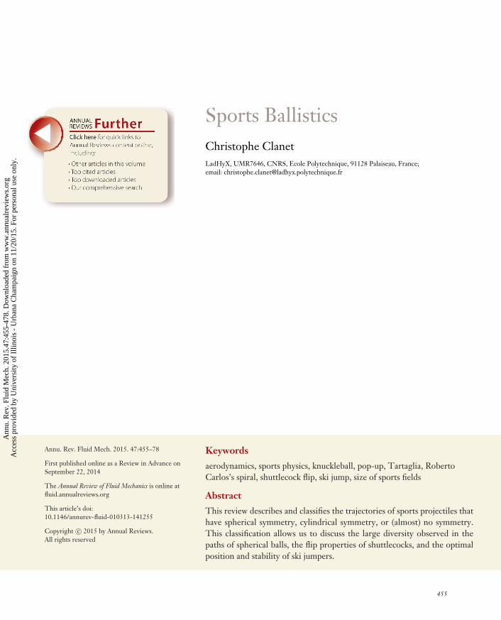
Here, following the advice of Frohlich (2011), we try to keep the tradition alive and addresssome questions about the trajectories of sports projectiles (Figure 1): Apart from parabolas, whattrajectories can be observed with spherical balls (Section 2)? What determines the size of sportsfields (Section 2.4.3)? How does one throw a knuckleball (Section 2.4.6)? Why do shuttlecocksflip (Section 3)? What is the optimal position for a ski jumper (Section 4)? What role does thesymmetry of the particle play in its trajectory (Sections 3 and 4)? To answer these questions, weregularly make reference to the work of famous pioneers, Mehta (1985) and de Mestre (1990).

2. SPHERICAL BALLS

For a homogeneous spherical ball of mass M and velocity U, the whole problem of the ball’strajectory is to solve the equation of motion:

MdUdt

= FG + FA(U), (1)

a b c

Figure 1Example of sports projectiles with different symmetries: (a) a soccer ball, which has spherical symmetry; (b) a shuttlecock, which hascylindrical symmetry; and (c) a ski jumper, who has (almost) no symmetry. Photo of Gregor Schlierenzauer by A. Furtner.

1The term tennis is from the French tenez, which can be translated as “take!”, a call from the server to the opponent, indicatingthat he or she is about to serve.

456 Clanet

Ann

u. R

ev. F

luid

Mec

h. 2

015.

47:4

55-4

78. D

ownl

oade

d fr

om w

ww

.ann

ualr

evie

ws.

org

Acc

ess

prov

ided

by

Uni

vers

ity o

f Il

linoi

s -

Urb

ana

Cha

mpa

ign

on 1

1/20

/15.

For

per

sona

l use

onl

y.

FL47CH19-Clanet ARI 18 November 2014 13:26

1

1Sp = FL/Mg

Dr = FD /Mg

f

a

b

c

d

e

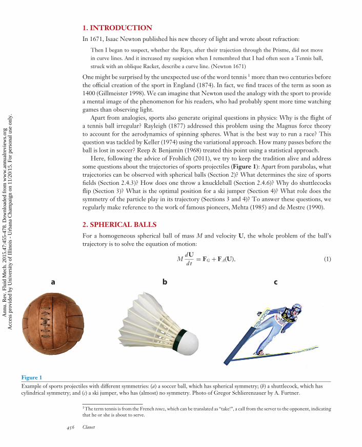
Figure 2Phase diagram of the different trajectories observed with spheres: (a) a parabola, (b) straight path, (c) knuckleball, (d ) Tartaglia curve,(e) spiral, and ( f ) pop-up.

where FG = Mg is the weight, and FA(U) is the aerodynamic force. To illustrate the diversityof the ballistic problem, I use the classical drag-lift decomposition of the aerodynamic force,FA = FD + FL. In this expression, FD stands for the drag (i.e., the part of the force aligned withthe velocity), and FL stands for the lift (i.e., the part of the force perpendicular to the velocity).

2.1. The Phase Diagram for the Trajectories

The different trajectories of particles submitted to gravity and aerodynamic forces can be discussedin the phase space (Dr = FD/M g, Sp = FL/Mg) presented in Figure 2: When gravity dominates(Dr � 1, Sp � 1), the trajectories reduce to parabolas (trajectory a in the figure) (Galilei 1638). Athigher velocities and without rotation (Dr � 1, Sp � 1), three different kinds of trajectories exist:straight lines (trajectory b), knuckleballs (trajectory c), and Tartaglia curves (trajectory d) (Tartaglia1537, Cohen et al. 2014a). When the ball spins (Dr � 1, Sp � 1), spirals are observed (trajectorye) (Dupeux et al. 2010). Finally, when the three forces are at play, loops (or pop-ups) appear(trajectory f) (McBeath et al. 2008). This section is devoted to the study of these different paths.

2.2. Characteristics of Ball Games

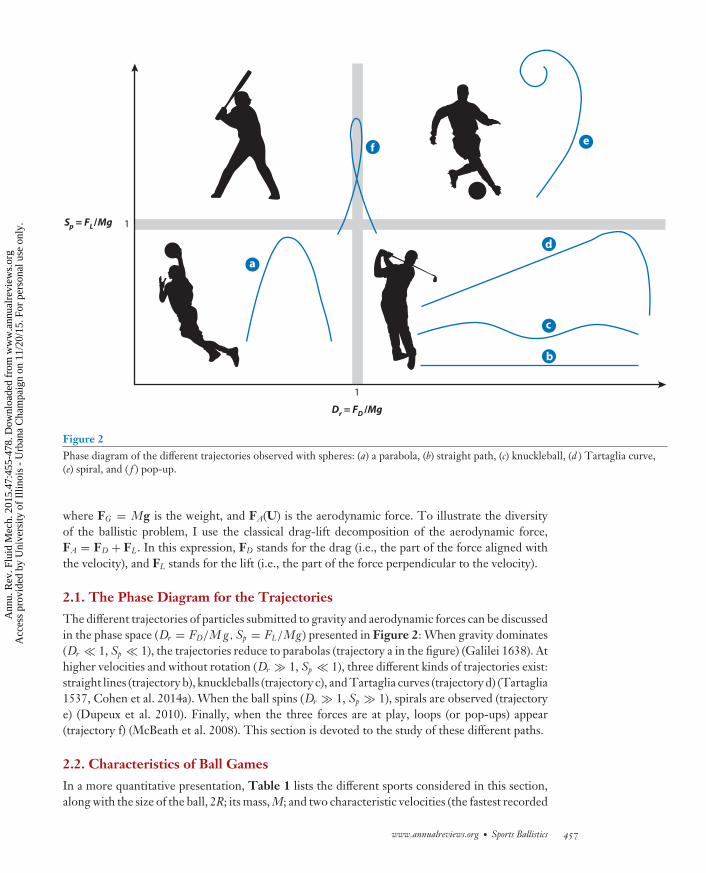
In a more quantitative presentation, Table 1 lists the different sports considered in this section,along with the size of the ball, 2R; its mass, M; and two characteristic velocities (the fastest recorded

www.annualreviews.org • Sports Ballistics 457

Ann

u. R

ev. F

luid

Mec

h. 2

015.

47:4

55-4

78. D

ownl

oade

d fr

om w

ww

.ann

ualr

evie

ws.

org

Acc

ess

prov

ided

by

Uni

vers

ity o

f Il

linoi

s -

Urb

ana

Cha

mpa

ign

on 1

1/20

/15.

For

per

sona

l use

onl

y.

FL47CH19-Clanet ARI 18 November 2014 13:26

Table 1 Characteristics of various sports projectiles

Sport

BadmintonTennis

Ping-pong

SquashJai alai

Golf

VolleyballSoccer

2R (cm)

6.06.5

4.0

4.06.5

4.2

2121

M (g)

5.0055.0

2.50

24.0120

45.0

210450

(m/s)Umax

13773.0

32.0

78.083.0

91.0

37.051.0

(m/s)U∞

6.7 3 × 104

22

10

3441

48

2030

(m/s)RΩ0

0.01910

17

3.10.20

7.7

5.39.1

CD

0.640.56

0.36

0.300.38

0.23

0.250.24

2RU∞/vRe =

1 × 105

3 × 104

1 × 105

2 × 105

2 × 105

4 × 105

5 × 105

FD /Mg

42011

10

5.44.1

3.6

3.42.9

FL /Mg

0.13

18

0.80.03

1.4

2.12.3

Softball

Baseball

CricketLacrosse

Handball

9.7

7.0

7.26.3

19

190

145

160143

450

47.0

54.0

53.050.0

27.0

33

40

4048

36

6.1

6.6

3.40.20

0.60

0.38

0.38

0.400.35

0.20

3 × 105

2 × 105

3 × 105

3 × 105

6 × 105

2.0

1.8

1.81.1

0.56

0.7

0.6

0.30.01

0.07Basketball 24 650 16.0 31 0.750.246 × 105 0.27 0.06

The diameter 2R and mass M are extracted from the official rules of the different federations. The sources for the maximum recorded speed Umax are asfollows: badminton (RIA Novosti 2013; http://en.wikipedia.org/wiki/Tan_Boon_Heong), tennis (http://en.wikipedia.org/wiki/Fastest_recorded_tennis_serves), ping-pong (Turberville 2003), squash (http://en.wikipedia.org/wiki/Cameron_Pilley), jai alai (http://en.wikipedia.org/wiki/Jai_alai), golf (http://en.wikipedia.org/wiki/Golf_ball), volleyball (Volleywood 2012), soccer (http://www.guinnessworldrecords.com), softball (Nathan2003, Russell 2008, Alam et al. 2012), baseball (eFastball.com 2011, Greenwald et al. 2001), lacrosse (http://www.guinnessworldrecords.com), handball(Gorostiaga et al. 2005), and basketball (Huston & Cesar 2003). The terminal velocities, U ∞, have been measured in a vertical wind tunnel (Cohen et al.2014a). The Reynolds number Re is calculated with an air viscosity of ν = 1.5 × 10−5 m2/s. The drag coefficient CD is linked to the mass and terminalvelocity via the relation CD = 2M g/(ρU 2

∞π R2). The data for the spin velocity are mainly extracted from Cottey (2002).

speed of the game, Umax, and the terminal velocity, U ∞). The table also includes badminton tostress its difference in velocity with the other sports. The terminal velocity is defined as thelevitating speed, that is, the speed for which the drag exactly equals the weight, FD(U ∞) = Mg.The corresponding Reynolds number (Re) is also listed in the table and is found to be of the orderof 105 for all sports. In this limit, we can write the drag force FD as

FD(U) = −12ρU USCD, (2)

where ρ is the density of air, S = π R2 is the cross-sectional area of the ball, and CD is the dragcoefficient. For the different sports, Table 1 lists the drag coefficient at the terminal velocity andpresents the maximal recorded spinning velocity (R�0), prior to the calculation of the reduceddrag, Dr = FD/M g, and reduced lift, Sp = FL/Mg. It is classical to use a formula similar toEquation 2 to calculate the lift: FL = 1/2ρU 2SCL. However, this formulation does not allow oneto determine the direction of the force and the link with the rotation of the ball. We thus use adifferent expression for the lift, based on the Blasius formula:

FL(U) = ρR3� ∧ UC�, (3)

where � is the spin vector and C� the spin coefficient. Using data from Nathan (2008), we evaluateC� ≈ 1.7 in the range R�0/U < 0.5, which holds for all the sports listed in Table 1. Equation 3can be used to compare the lift force to the weight in the table. A deeper discussion on the Magnuseffect in ball games can be found in the work of Bush (2013).

458 Clanet

Ann

u. R

ev. F

luid

Mec

h. 2

015.

47:4

55-4

78. D

ownl

oade

d fr

om w

ww

.ann

ualr

evie

ws.

org

Acc

ess

prov

ided

by

Uni

vers

ity o

f Il

linoi

s -

Urb

ana

Cha

mpa

ign

on 1

1/20

/15.

For

per

sona

l use

onl

y.

FL47CH19-Clanet ARI 18 November 2014 13:26

2.3. Classification of Ball Games

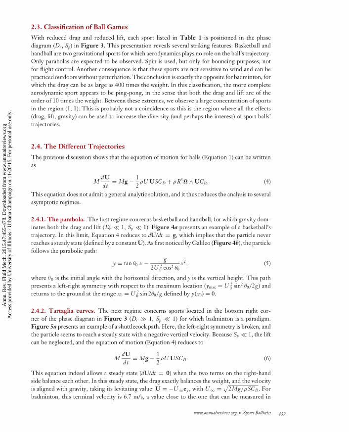
With reduced drag and reduced lift, each sport listed in Table 1 is positioned in the phasediagram (Dr , Sp) in Figure 3. This presentation reveals several striking features: Basketball andhandball are two gravitational sports for which aerodynamics plays no role on the ball’s trajectory.Only parabolas are expected to be observed. Spin is used, but only for bouncing purposes, notfor flight control. Another consequence is that these sports are not sensitive to wind and can bepracticed outdoors without perturbation. The conclusion is exactly the opposite for badminton, forwhich the drag can be as large as 400 times the weight. In this classification, the more completeaerodynamic sport appears to be ping-pong, in the sense that both the drag and lift are of theorder of 10 times the weight. Between these extremes, we observe a large concentration of sportsin the region (1, 1). This is probably not a coincidence as this is the region where all the effects(drag, lift, gravity) can be used to increase the diversity (and perhaps the interest) of sport balls’trajectories.

2.4. The Different Trajectories

The previous discussion shows that the equation of motion for balls (Equation 1) can be writtenas

MdUdt

= Mg − 12ρU USCD + ρR3� ∧ UC�. (4)

This equation does not admit a general analytic solution, and it thus reduces the analysis to severalasymptotic regimes.

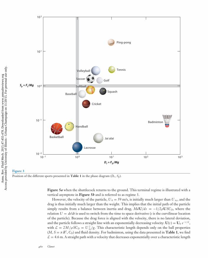
2.4.1. The parabola. The first regime concerns basketball and handball, for which gravity dom-inates both the drag and lift (Dr � 1, Sp � 1). Figure 4a presents an example of a basketball’strajectory. In this limit, Equation 4 reduces to dU/dt = g, which implies that the particle neverreaches a steady state (defined by a constant U). As first noticed by Galileo (Figure 4b), the particlefollows the parabolic path:

y = tan θ0 x − g2U 2

0 cos2 θ0x2, (5)

where θ0 is the initial angle with the horizontal direction, and y is the vertical height. This pathpresents a left-right symmetry with respect to the maximum location (ymax = U 2

0 sin2 θ0/2g) andreturns to the ground at the range x0 = U 2

0 sin 2θ0/g defined by y(x0) = 0.

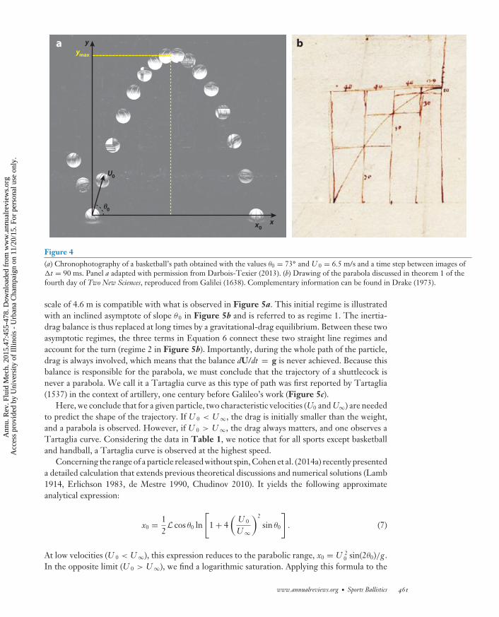
2.4.2. Tartaglia curves. The next regime concerns sports located in the bottom right cor-ner of the phase diagram in Figure 3 (Dr � 1, Sp � 1) for which badminton is a paradigm.Figure 5a presents an example of a shuttlecock path. Here, the left-right symmetry is broken, andthe particle seems to reach a steady state with a negative vertical velocity. Because Sp � 1, the liftcan be neglected, and the equation of motion (Equation 4) reduces to

MdUdt

= Mg − 12ρU USCD. (6)

This equation indeed allows a steady state (dU/dt = 0) when the two terms on the right-handside balance each other. In this steady state, the drag exactly balances the weight, and the velocityis aligned with gravity, taking its levitating value: U = −U ∞ey , with U ∞ = √

2Mg/ρSCD. Forbadminton, this terminal velocity is 6.7 m/s, a value close to the one that can be measured in

www.annualreviews.org • Sports Ballistics 459

Ann

u. R

ev. F

luid

Mec

h. 2

015.

47:4

55-4

78. D

ownl

oade

d fr

om w

ww

.ann

ualr

evie

ws.

org

Acc

ess

prov

ided

by

Uni

vers

ity o

f Il

linoi

s -

Urb

ana

Cha

mpa

ign

on 1

1/20

/15.

For

per

sona

l use

onl

y.

FL47CH19-Clanet ARI 18 November 2014 13:26

10 –1 10 0 10 1 10 2

Ping-pong

Tennis

Golf

Squash

Cricket

Handball

Jai alai

Volleyball

Soccer

Softball

Baseball

Basketball

Lacrosse

Badminton

10 2

10 1

10 0

10 –1

10 –2

10 3

Sp = FL/Mg

Dr = FD /Mg

Figure 3Position of the different sports presented in Table 1 in the phase diagram (Dr , Sp).

Figure 5a when the shuttlecock returns to the ground. This terminal regime is illustrated with avertical asymptote in Figure 5b and is referred to as regime 3.

However, the velocity of the particle, U 0 = 59 m/s, is initially much larger than U ∞, and thedrag is thus initially much larger than the weight. This implies that the initial path of the particlesimply results from a balance between inertia and drag, MdU/ds = −1/2ρUSCD, where therelation U = ds/dt is used to switch from the time to space derivative (s is the curvilinear locationof the particle). Because the drag force is aligned with the velocity, there is no lateral deviation,and the particle follows a straight line with an exponentially decreasing velocity: U(s ) = U0 e−s /L,with L = 2M /ρSCD = U 2

∞/g. This characteristic length depends only on the ball properties(M, S = π R2, CD) and fluid density. For badminton, using the data presented in Table 1, we findL = 4.6 m. A straight path with a velocity that decreases exponentially over a characteristic length

460 Clanet

Ann

u. R

ev. F

luid

Mec

h. 2

015.

47:4

55-4

78. D

ownl

oade

d fr

om w

ww

.ann

ualr

evie

ws.

org

Acc

ess

prov

ided

by

Uni

vers

ity o

f Il

linoi

s -

Urb

ana

Cha

mpa

ign

on 1

1/20

/15.

For

per

sona

l use

onl

y.

FL47CH19-Clanet ARI 18 November 2014 13:26

ymax y

x

a b

U0

x0

θ0

Figure 4(a) Chronophotography of a basketball’s path obtained with the values θ0 = 73◦ and U 0 = 6.5 m/s and a time step between images of�t = 90 ms. Panel a adapted with permission from Darbois-Texier (2013). (b) Drawing of the parabola discussed in theorem 1 of thefourth day of Two New Sciences, reproduced from Galilei (1638). Complementary information can be found in Drake (1973).

scale of 4.6 m is compatible with what is observed in Figure 5a. This initial regime is illustratedwith an inclined asymptote of slope θ0 in Figure 5b and is referred to as regime 1. The inertia-drag balance is thus replaced at long times by a gravitational-drag equilibrium. Between these twoasymptotic regimes, the three terms in Equation 6 connect these two straight line regimes andaccount for the turn (regime 2 in Figure 5b). Importantly, during the whole path of the particle,drag is always involved, which means that the balance dU/dt = g is never achieved. Because thisbalance is responsible for the parabola, we must conclude that the trajectory of a shuttlecock isnever a parabola. We call it a Tartaglia curve as this type of path was first reported by Tartaglia(1537) in the context of artillery, one century before Galileo’s work (Figure 5c).

Here, we conclude that for a given particle, two characteristic velocities (U0 and U∞) are neededto predict the shape of the trajectory. If U 0 < U ∞, the drag is initially smaller than the weight,and a parabola is observed. However, if U 0 > U ∞, the drag always matters, and one observes aTartaglia curve. Considering the data in Table 1, we notice that for all sports except basketballand handball, a Tartaglia curve is observed at the highest speed.

Concerning the range of a particle released without spin, Cohen et al. (2014a) recently presenteda detailed calculation that extends previous theoretical discussions and numerical solutions (Lamb1914, Erlichson 1983, de Mestre 1990, Chudinov 2010). It yields the following approximateanalytical expression:

x0 = 12L cos θ0 ln

[1 + 4

(U 0

U ∞

)2

sin θ0

]. (7)

At low velocities (U 0 < U ∞), this expression reduces to the parabolic range, x0 = U 20 sin(2θ0)/g.

In the opposite limit (U 0 > U ∞), we find a logarithmic saturation. Applying this formula to the

www.annualreviews.org • Sports Ballistics 461

Ann

u. R

ev. F

luid

Mec

h. 2

015.

47:4

55-4

78. D

ownl

oade

d fr

om w

ww

.ann

ualr

evie

ws.

org

Acc

ess

prov

ided

by

Uni

vers

ity o

f Il

linoi

s -

Urb

ana

Cha

mpa

ign

on 1

1/20

/15.

For

per

sona

l use

onl

y.

FL47CH19-Clanet ARI 18 November 2014 13:26

12

3

x

y

0

9 m

a

b

c

U0

U∞

x0

θ0

Figure 5(a) Chronophotography of a shuttlecock’s path obtained with the values θ0 = 52◦ and U 0 = 59 m/s and a time step between images of�t = 50 ms. With the first two tracks, the image shows 40 m/s, but the shuttlecock has already decelerated. Panel a adapted withpermission from Darbois-Texier et al. (2014). (b) Schematic illustration of the asymptotic regimes of a Tartaglia curve. (c) Illustration ofa bullet path from the treatise Nova Scientia. Panel c reproduced from Tartaglia (1537).

trajectory presented in Figure 5a, we get x0 ≈ 8.5 m, which is compatible with the observedrange. For comparison, the parabolic range in this case is U 2

0 sin(2θ0)/g ≈ 244 m.From Equation 7, the optimal angle, θmax, that maximizes the range and the corresponding

maximum range xmax = x0(U max, θmax) can be calculated as

xmax = 12L cos θmax ln

[1 + 4

(U max

U ∞

)2

sin θmax

], (8)

with

θmax = arctan

√(U max/U ∞)2

[1 + (U max/U ∞)2] ln[1 + (U max/U ∞)2]. (9)

In the limit U max/U ∞ � 1, Equation 8 reduces to xmax = 2U 2max/g sin θmax cos θmax, whereas

Equation 9 leads to θmax = arctan(1). We thus recover the parabolic regime in which the rangeis maximized with θmax = π/4 and takes the value xmax = U 2

max/g. In the opposite limit in whichU max/U ∞ � 1, the maximal value of the range weakly increases with the velocity while the optimalangle decreases, as studied by Cohen et al. (2014a). What is important to realize is that once thevelocities U max and U ∞ are known, the problem of the maximal range is solved, as Equation 9provides the optimal angle and Equation 8 provides the maximal range

(L = U 2

∞/g). In sports,

U ∞ is fixed by the choice of the ball (shape and mass), and U max is fixed by the launch method(e.g., throw, bat, racket, kick).

462 Clanet

Ann

u. R

ev. F

luid

Mec

h. 2

015.

47:4

55-4

78. D

ownl

oade

d fr

om w

ww

.ann

ualr

evie

ws.

org

Acc

ess

prov

ided

by

Uni

vers

ity o

f Il

linoi

s -

Urb

ana

Cha

mpa

ign

on 1

1/20

/15.

For

per

sona

l use

onl

y.

FL47CH19-Clanet ARI 18 November 2014 13:26

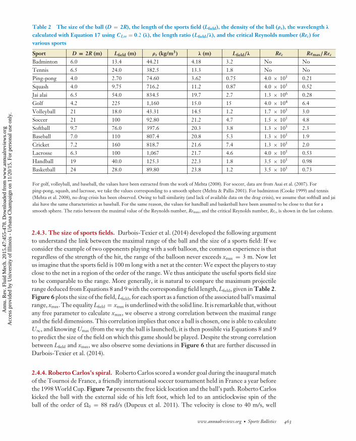
Table 2 The size of the ball (D = 2R), the length of the sports field (Lfield), the density of the ball (ρs), the wavelength λ

calculated with Equation 17 using CLm = 0.2 (λ), the length ratio (Lfield/λ), and the critical Reynolds number (Rec) forvarious sports

Sport D = 2R (m) Lfield (m) ρs (kg/m3) λ (m) Lfield/λ Rec Remax/Rec

Badminton 6.0 13.4 44.21 4.18 3.2 No NoTennis 6.5 24.0 382.5 13.3 1.8 No NoPing-pong 4.0 2.70 74.60 3.62 0.75 4.0 × 105 0.21Squash 4.0 9.75 716.2 11.2 0.87 4.0 × 105 0.52Jai alai 6.5 54.0 834.5 19.7 2.7 1.3 × 106 0.28Golf 4.2 225 1,160 15.0 15 4.0 × 104 6.4Volleyball 21 18.0 43.31 14.5 1.2 1.7 × 105 3.0Soccer 21 100 92.80 21.2 4.7 1.5 × 105 4.8Softball 9.7 76.0 397.6 20.3 3.8 1.3 × 105 2.3Baseball 7.0 110 807.4 20.8 5.3 1.3 × 105 1.9Cricket 7.2 160 818.7 21.6 7.4 1.3 × 105 2.0Lacrosse 6.3 100 1,067 21.7 4.6 4.0 × 105 0.53Handball 19 40.0 125.3 22.3 1.8 3.5 × 105 0.98Basketball 24 28.0 89.80 23.8 1.2 3.5 × 105 0.73

For golf, volleyball, and baseball, the values have been extracted from the work of Mehta (2008). For soccer, data are from Asai et al. (2007). Forping-pong, squash, and lacrosse, we take the values corresponding to a smooth sphere (Mehta & Pallis 2001). For badminton (Cooke 1999) and tennis(Mehta et al. 2008), no drag crisis has been observed. Owing to ball similarity (and lack of available data on the drag crisis), we assume that softball and jaialai have the same characteristics as baseball. For the same reason, the values for handball and basketball have been assumed to be close to that for asmooth sphere. The ratio between the maximal value of the Reynolds number, Remax, and the critical Reynolds number, Rec , is shown in the last column.

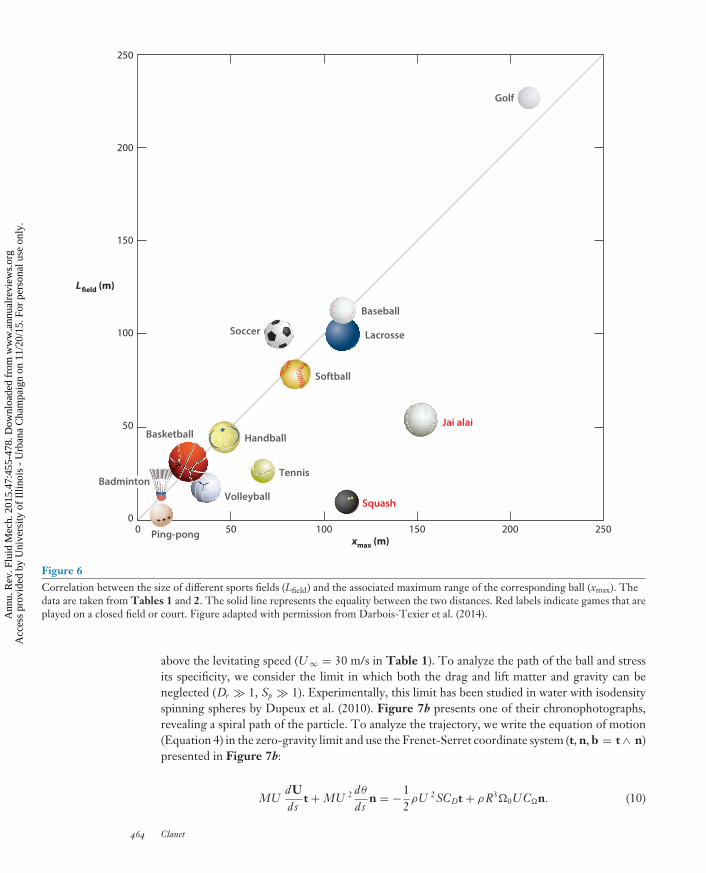
2.4.3. The size of sports fields. Darbois-Texier et al. (2014) developed the following argumentto understand the link between the maximal range of the ball and the size of a sports field: If weconsider the example of two opponents playing with a soft balloon, the common experience is thatregardless of the strength of the hit, the range of the balloon never exceeds xmax = 3 m. Now letus imagine that the sports field is 100 m long with a net at the center: We expect the players to stayclose to the net in a region of the order of the range. We thus anticipate the useful sports field sizeto be comparable to the range. More generally, it is natural to compare the maximum projectilerange deduced from Equations 8 and 9 with the corresponding field length, Lfield, given in Table 2.Figure 6 plots the size of the field, Lfield, for each sport as a function of the associated ball’s maximalrange, xmax. The equality Lfield = xmax is underlined with the solid line. It is remarkable that, withoutany free parameter to calculate xmax, we observe a strong correlation between the maximal rangeand the field dimensions. This correlation implies that once a ball is chosen, one is able to calculateU∞, and knowing Umax (from the way the ball is launched), it is then possible via Equations 8 and 9to predict the size of the field on which this game should be played. Despite the strong correlationbetween Lfield and xmax, we also observe some deviations in Figure 6 that are further discussed inDarbois-Texier et al. (2014).

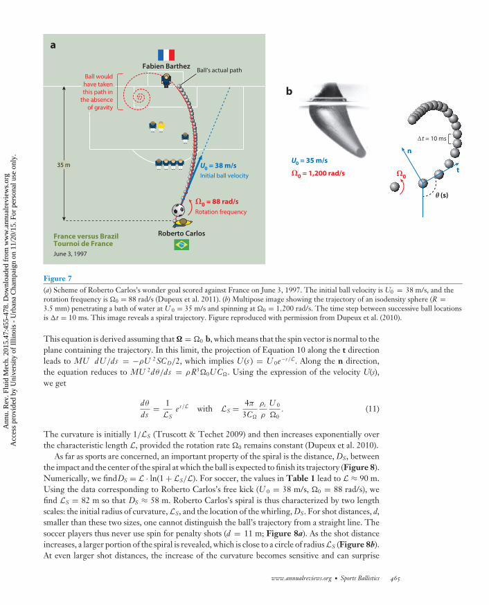
2.4.4. Roberto Carlos’s spiral. Roberto Carlos scored a wonder goal during the inaugural matchof the Tournoi de France, a friendly international soccer tournament held in France a year beforethe 1998 World Cup. Figure 7a presents the free kick location and the ball’s path. Roberto Carloskicked the ball with the external side of his left foot, which led to an anticlockwise spin of theball of the order of �0 = 88 rad/s (Dupeux et al. 2011). The velocity is close to 40 m/s, well

www.annualreviews.org • Sports Ballistics 463

Ann

u. R

ev. F

luid

Mec

h. 2

015.

47:4

55-4

78. D

ownl

oade

d fr

om w

ww

.ann

ualr

evie

ws.

org

Acc

ess

prov

ided

by

Uni

vers

ity o

f Il

linoi

s -

Urb

ana

Cha

mpa

ign

on 1

1/20

/15.

For

per

sona

l use

onl

y.

FL47CH19-Clanet ARI 18 November 2014 13:26

0 50 100 150 200Ping-pong

Tennis

Golf

Squash

Handball

Jai alai

Volleyball

Soccer

Softball

Baseball

Basketball

Lacrosse

Badminton

250

200

150

100

50

0250

xmax (m)

Lfield (m)

Figure 6Correlation between the size of different sports fields (Lfield) and the associated maximum range of the corresponding ball (xmax). Thedata are taken from Tables 1 and 2. The solid line represents the equality between the two distances. Red labels indicate games that areplayed on a closed field or court. Figure adapted with permission from Darbois-Texier et al. (2014).

above the levitating speed (U ∞ = 30 m/s in Table 1). To analyze the path of the ball and stressits specificity, we consider the limit in which both the drag and lift matter and gravity can beneglected (Dr � 1, Sp � 1). Experimentally, this limit has been studied in water with isodensityspinning spheres by Dupeux et al. (2010). Figure 7b presents one of their chronophotographs,revealing a spiral path of the particle. To analyze the trajectory, we write the equation of motion(Equation 4) in the zero-gravity limit and use the Frenet-Serret coordinate system (t, n, b = t ∧ n)presented in Figure 7b:

MUdUds

t + MU 2 dθ

dsn = −1

2ρU 2SCDt + ρR3�0UC�n. (10)

464 Clanet

Ann

u. R

ev. F

luid

Mec

h. 2

015.

47:4

55-4

78. D

ownl

oade

d fr

om w

ww

.ann

ualr

evie

ws.

org

Acc

ess

prov

ided

by

Uni

vers

ity o

f Il

linoi

s -

Urb

ana

Cha

mpa

ign

on 1

1/20

/15.

For

per

sona

l use

onl

y.

FL47CH19-Clanet ARI 18 November 2014 13:26

France versus BrazilTournoi de FranceJune 3, 1997

a

U0 = 38 m/sInitial ball velocity

Rotation frequency

Roberto Carlos

Fabien Barthez

Ω0 = 88 rad/s

Ball would

have taken

this path in

the absence

of gravity

Ball’s actual path

b

U0 = 35 m/s

Ω0 = 1,200 rad/s

Δt = 10 ms

Ω0

θ (s)

t

n

35 m

Figure 7(a) Scheme of Roberto Carlos’s wonder goal scored against France on June 3, 1997. The initial ball velocity is U0 = 38 m/s, and therotation frequency is �0 = 88 rad/s (Dupeux et al. 2011). (b) Multipose image showing the trajectory of an isodensity sphere (R =3.5 mm) penetrating a bath of water at U 0 = 35 m/s and spinning at �0 = 1,200 rad/s. The time step between successive ball locationsis �t = 10 ms. This image reveals a spiral trajectory. Figure reproduced with permission from Dupeux et al. (2010).

This equation is derived assuming that � = �0 b, which means that the spin vector is normal to theplane containing the trajectory. In this limit, the projection of Equation 10 along the t directionleads to MU dU/ds = −ρU 2SCD/2, which implies U (s ) = U 0e−s /L. Along the n direction,the equation reduces to MU 2dθ/ds = ρR3�0UC�. Using the expression of the velocity U(s),we get

dθ

ds= 1

LSe s /L with LS = 4π

3C�

ρs

ρ

U 0

�0. (11)

The curvature is initially 1/LS (Truscott & Techet 2009) and then increases exponentially overthe characteristic length L, provided the rotation rate �0 remains constant (Dupeux et al. 2010).

As far as sports are concerned, an important property of the spiral is the distance, DS, betweenthe impact and the center of the spiral at which the ball is expected to finish its trajectory (Figure 8).Numerically, we findDS = L · ln(1 + LS/L). For soccer, the values in Table 1 lead to L ≈ 90 m.Using the data corresponding to Roberto Carlos’s free kick (U 0 = 38 m/s, �0 = 88 rad/s), wefind LS = 82 m so that DS ≈ 58 m. Roberto Carlos’s spiral is thus characterized by two lengthscales: the initial radius of curvature, LS, and the location of the whirling, DS. For shot distances, d,smaller than these two sizes, one cannot distinguish the ball’s trajectory from a straight line. Thesoccer players thus never use spin for penalty shots (d = 11 m; Figure 8a). As the shot distanceincreases, a larger portion of the spiral is revealed, which is close to a circle of radiusLS (Figure 8b).At even larger shot distances, the increase of the curvature becomes sensitive and can surprise

www.annualreviews.org • Sports Ballistics 465

Ann

u. R

ev. F

luid

Mec

h. 2

015.

47:4

55-4

78. D

ownl

oade

d fr

om w

ww

.ann

ualr

evie

ws.

org

Acc

ess

prov

ided

by

Uni

vers

ity o

f Il

linoi

s -

Urb

ana

Cha

mpa

ign

on 1

1/20

/15.

For

per

sona

l use

onl

y.

FL47CH19-Clanet ARI 18 November 2014 13:26

S

a b c

U0

d = 11 md

DS

I N C R E A S I N G L E N G T H O F S H O T

Ω0

d = 18 md d = 35 md

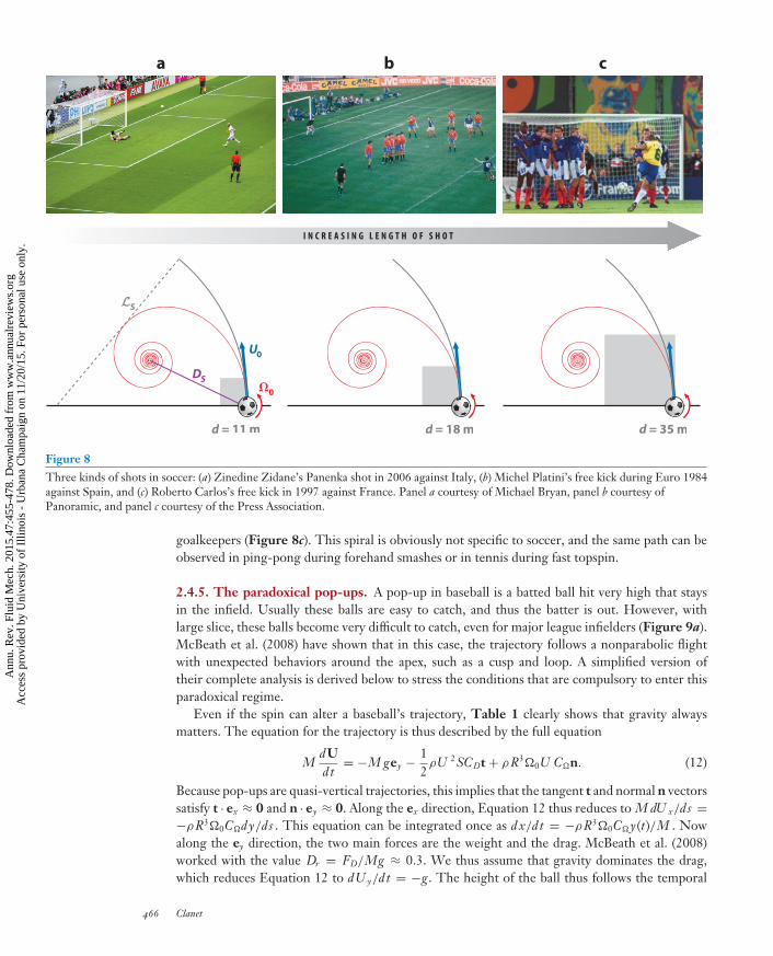
Figure 8Three kinds of shots in soccer: (a) Zinedine Zidane’s Panenka shot in 2006 against Italy, (b) Michel Platini’s free kick during Euro 1984against Spain, and (c) Roberto Carlos’s free kick in 1997 against France. Panel a courtesy of Michael Bryan, panel b courtesy ofPanoramic, and panel c courtesy of the Press Association.

goalkeepers (Figure 8c). This spiral is obviously not specific to soccer, and the same path can beobserved in ping-pong during forehand smashes or in tennis during fast topspin.

2.4.5. The paradoxical pop-ups. A pop-up in baseball is a batted ball hit very high that staysin the infield. Usually these balls are easy to catch, and thus the batter is out. However, withlarge slice, these balls become very difficult to catch, even for major league infielders (Figure 9a).McBeath et al. (2008) have shown that in this case, the trajectory follows a nonparabolic flightwith unexpected behaviors around the apex, such as a cusp and loop. A simplified version oftheir complete analysis is derived below to stress the conditions that are compulsory to enter thisparadoxical regime.

Even if the spin can alter a baseball’s trajectory, Table 1 clearly shows that gravity alwaysmatters. The equation for the trajectory is thus described by the full equation

MdUdt

= −M gey − 12ρU 2SCDt + ρR3�0U C�n. (12)

Because pop-ups are quasi-vertical trajectories, this implies that the tangent t and normal n vectorssatisfy t · ex ≈ 0 and n · ey ≈ 0. Along the ex direction, Equation 12 thus reduces to M dU x/ds =−ρR3�0C�d y/ds . This equation can be integrated once as d x/dt = −ρR3�0C�y(t)/M . Nowalong the ey direction, the two main forces are the weight and the drag. McBeath et al. (2008)worked with the value Dr = FD/Mg ≈ 0.3. We thus assume that gravity dominates the drag,which reduces Equation 12 to dU y/dt = −g. The height of the ball thus follows the temporal

466 Clanet

Ann

u. R

ev. F

luid

Mec

h. 2

015.

47:4

55-4

78. D

ownl

oade

d fr

om w

ww

.ann

ualr

evie

ws.

org

Acc

ess

prov

ided

by

Uni

vers

ity o

f Il

linoi

s -

Urb

ana

Cha

mpa

ign

on 1

1/20

/15.

For

per

sona

l use

onl

y.

FL47CH19-Clanet ARI 18 November 2014 13:26

gx/U20

gy/U20

Gravity 0.5

0.4

0.3

0.2

0.1

00 0.05 0.10 1.15

SP = 0SP = 00.1760.1760.220.22

a b c

θ (s)

x

y

0

Ω0

tn

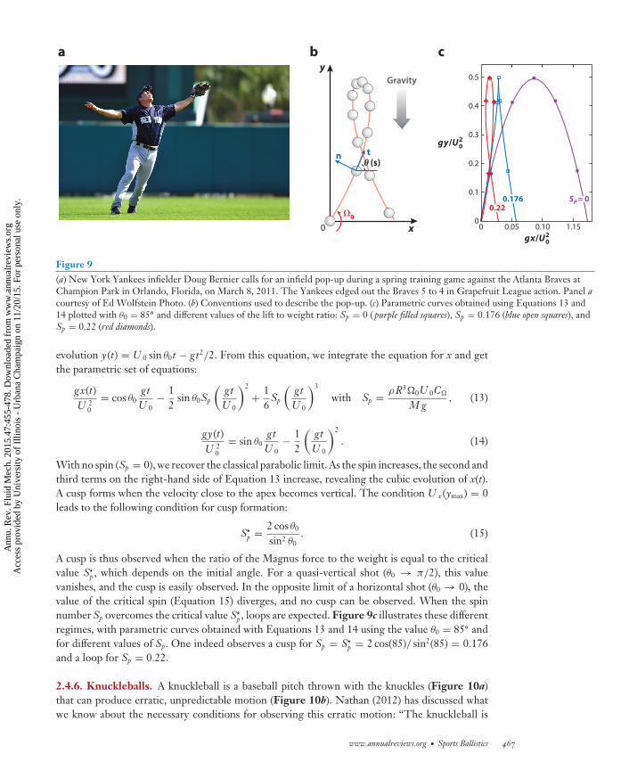
Figure 9(a) New York Yankees infielder Doug Bernier calls for an infield pop-up during a spring training game against the Atlanta Braves atChampion Park in Orlando, Florida, on March 8, 2011. The Yankees edged out the Braves 5 to 4 in Grapefruit League action. Panel acourtesy of Ed Wolfstein Photo. (b) Conventions used to describe the pop-up. (c) Parametric curves obtained using Equations 13 and14 plotted with θ0 = 85◦ and different values of the lift to weight ratio: Sp = 0 ( purple filled squares), Sp = 0.176 (blue open squares), andSp = 0.22 (red diamonds).

evolution y(t) = U 0 sin θ0t − gt2/2. From this equation, we integrate the equation for x and getthe parametric set of equations:

gx(t)U 2

0= cos θ0

gtU 0

− 12

sin θ0Sp

(gtU 0

)2

+ 16

Sp

(gtU 0

)3

with Sp = ρR3�0U 0C�

M g, (13)

gy(t)U 2

0= sin θ0

gtU 0

− 12

(gtU 0

)2

. (14)

With no spin (Sp = 0), we recover the classical parabolic limit. As the spin increases, the second andthird terms on the right-hand side of Equation 13 increase, revealing the cubic evolution of x(t).A cusp forms when the velocity close to the apex becomes vertical. The condition U x(ymax) = 0leads to the following condition for cusp formation:

S�p = 2 cos θ0

sin2 θ0. (15)

A cusp is thus observed when the ratio of the Magnus force to the weight is equal to the criticalvalue S�

p , which depends on the initial angle. For a quasi-vertical shot (θ0 → π/2), this valuevanishes, and the cusp is easily observed. In the opposite limit of a horizontal shot (θ0 → 0), thevalue of the critical spin (Equation 15) diverges, and no cusp can be observed. When the spinnumber Sp overcomes the critical value S�

p , loops are expected. Figure 9c illustrates these differentregimes, with parametric curves obtained with Equations 13 and 14 using the value θ0 = 85◦ andfor different values of Sp. One indeed observes a cusp for Sp = S�

p = 2 cos(85)/ sin2(85) = 0.176and a loop for Sp = 0.22.

2.4.6. Knuckleballs. A knuckleball is a baseball pitch thrown with the knuckles (Figure 10a)that can produce erratic, unpredictable motion (Figure 10b). Nathan (2012) has discussed whatwe know about the necessary conditions for observing this erratic motion: “The knuckleball is

www.annualreviews.org • Sports Ballistics 467

Ann

u. R

ev. F

luid

Mec

h. 2

015.

47:4

55-4

78. D

ownl

oade

d fr

om w

ww

.ann

ualr

evie

ws.

org

Acc

ess

prov

ided

by

Uni

vers

ity o

f Il

linoi

s -

Urb

ana

Cha

mpa

ign

on 1

1/20

/15.

For

per

sona

l use

onl

y.

FL47CH19-Clanet ARI 18 November 2014 13:26

a b

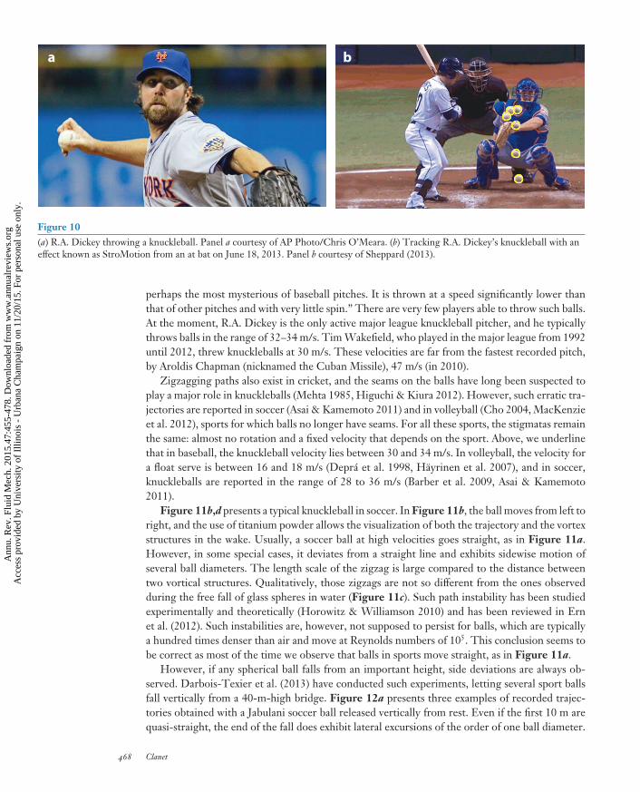
Figure 10(a) R.A. Dickey throwing a knuckleball. Panel a courtesy of AP Photo/Chris O’Meara. (b) Tracking R.A. Dickey’s knuckleball with aneffect known as StroMotion from an at bat on June 18, 2013. Panel b courtesy of Sheppard (2013).

perhaps the most mysterious of baseball pitches. It is thrown at a speed significantly lower thanthat of other pitches and with very little spin.” There are very few players able to throw such balls.At the moment, R.A. Dickey is the only active major league knuckleball pitcher, and he typicallythrows balls in the range of 32–34 m/s. Tim Wakefield, who played in the major league from 1992until 2012, threw knuckleballs at 30 m/s. These velocities are far from the fastest recorded pitch,by Aroldis Chapman (nicknamed the Cuban Missile), 47 m/s (in 2010).

Zigzagging paths also exist in cricket, and the seams on the balls have long been suspected toplay a major role in knuckleballs (Mehta 1985, Higuchi & Kiura 2012). However, such erratic tra-jectories are reported in soccer (Asai & Kamemoto 2011) and in volleyball (Cho 2004, MacKenzieet al. 2012), sports for which balls no longer have seams. For all these sports, the stigmatas remainthe same: almost no rotation and a fixed velocity that depends on the sport. Above, we underlinethat in baseball, the knuckleball velocity lies between 30 and 34 m/s. In volleyball, the velocity fora float serve is between 16 and 18 m/s (Depra et al. 1998, Hayrinen et al. 2007), and in soccer,knuckleballs are reported in the range of 28 to 36 m/s (Barber et al. 2009, Asai & Kamemoto2011).

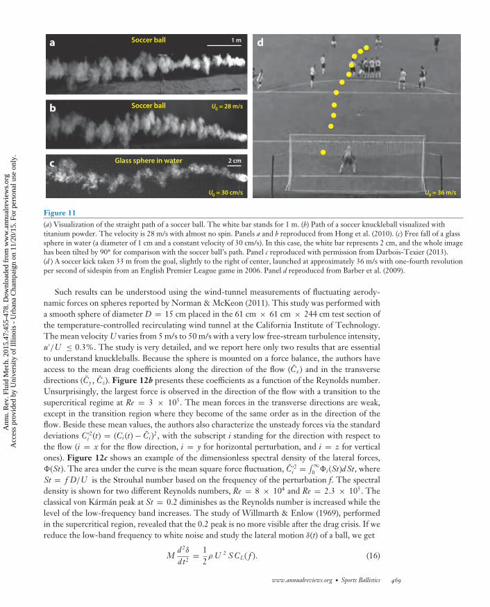
Figure 11b,d presents a typical knuckleball in soccer. In Figure 11b, the ball moves from left toright, and the use of titanium powder allows the visualization of both the trajectory and the vortexstructures in the wake. Usually, a soccer ball at high velocities goes straight, as in Figure 11a.However, in some special cases, it deviates from a straight line and exhibits sidewise motion ofseveral ball diameters. The length scale of the zigzag is large compared to the distance betweentwo vortical structures. Qualitatively, those zigzags are not so different from the ones observedduring the free fall of glass spheres in water (Figure 11c). Such path instability has been studiedexperimentally and theoretically (Horowitz & Williamson 2010) and has been reviewed in Ernet al. (2012). Such instabilities are, however, not supposed to persist for balls, which are typicallya hundred times denser than air and move at Reynolds numbers of 105. This conclusion seems tobe correct as most of the time we observe that balls in sports move straight, as in Figure 11a.

However, if any spherical ball falls from an important height, side deviations are always ob-served. Darbois-Texier et al. (2013) have conducted such experiments, letting several sport ballsfall vertically from a 40-m-high bridge. Figure 12a presents three examples of recorded trajec-tories obtained with a Jabulani soccer ball released vertically from rest. Even if the first 10 m arequasi-straight, the end of the fall does exhibit lateral excursions of the order of one ball diameter.

468 Clanet

Ann

u. R

ev. F

luid

Mec

h. 2

015.

47:4

55-4

78. D

ownl

oade

d fr

om w

ww

.ann

ualr

evie

ws.

org

Acc

ess

prov

ided

by

Uni

vers

ity o

f Il

linoi

s -

Urb

ana

Cha

mpa

ign

on 1

1/20

/15.

For

per

sona

l use

onl

y.

FL47CH19-Clanet ARI 18 November 2014 13:26

1 ma d

b

c

Soccer ball

Soccer ball

Glass sphere in water 2 cm

U0 = 28 m/s

U0 = 36 m/sU0 = 30 cm/s

Figure 11(a) Visualization of the straight path of a soccer ball. The white bar stands for 1 m. (b) Path of a soccer knuckleball visualized withtitanium powder. The velocity is 28 m/s with almost no spin. Panels a and b reproduced from Hong et al. (2010). (c) Free fall of a glasssphere in water (a diameter of 1 cm and a constant velocity of 30 cm/s). In this case, the white bar represents 2 cm, and the whole imagehas been tilted by 90◦ for comparison with the soccer ball’s path. Panel c reproduced with permission from Darbois-Texier (2013).(d ) A soccer kick taken 33 m from the goal, slightly to the right of center, launched at approximately 36 m/s with one-fourth revolutionper second of sidespin from an English Premier League game in 2006. Panel d reproduced from Barber et al. (2009).

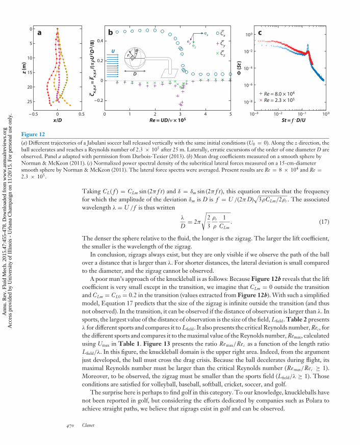
Such results can be understood using the wind-tunnel measurements of fluctuating aerody-namic forces on spheres reported by Norman & McKeon (2011). This study was performed witha smooth sphere of diameter D = 15 cm placed in the 61 cm × 61 cm × 244 cm test section ofthe temperature-controlled recirculating wind tunnel at the California Institute of Technology.The mean velocity U varies from 5 m/s to 50 m/s with a very low free-stream turbulence intensity,u′/U ≤ 0.3%. The study is very detailed, and we report here only two results that are essentialto understand knuckleballs. Because the sphere is mounted on a force balance, the authors haveaccess to the mean drag coefficients along the direction of the flow (Cx) and in the transversedirections (Cy , Cz). Figure 12b presents these coefficients as a function of the Reynolds number.Unsurprisingly, the largest force is observed in the direction of the flow with a transition to thesupercritical regime at Re = 3 × 105. The mean forces in the transverse directions are weak,except in the transition region where they become of the same order as in the direction of theflow. Beside these mean values, the authors also characterize the unsteady forces via the standarddeviations C ′2

i (t) = (Ci (t) − Ci )2, with the subscript i standing for the direction with respect tothe flow (i = x for the flow direction, i = y for horizontal perturbation, and i = z for verticalones). Figure 12c shows an example of the dimensionless spectral density of the lateral forces,(St). The area under the curve is the mean square force fluctuation, C ′2

i = ∫ ∞0 i (St)d St, where

St = f D/U is the Strouhal number based on the frequency of the perturbation f. The spectraldensity is shown for two different Reynolds numbers, Re = 8 × 104 and Re = 2.3 × 105. Theclassical von Karman peak at St = 0.2 diminishes as the Reynolds number is increased while thelevel of the low-frequency band increases. The study of Willmarth & Enlow (1969), performedin the supercritical region, revealed that the 0.2 peak is no more visible after the drag crisis. If wereduce the low-band frequency to white noise and study the lateral motion δ(t) of a ball, we get

Md 2δ

dt2= 1

2ρ U 2 S CL( f ). (16)

www.annualreviews.org • Sports Ballistics 469

Ann

u. R

ev. F

luid

Mec

h. 2

015.

47:4

55-4

78. D

ownl

oade

d fr

om w

ww

.ann

ualr

evie

ws.

org

Acc

ess

prov

ided

by

Uni

vers

ity o

f Il

linoi

s -

Urb

ana

Cha

mpa

ign

on 1

1/20

/15.

For

per

sona

l use

onl

y.

FL47CH19-Clanet ARI 18 November 2014 13:26

θθφφ

U

D

r

C x,y,

z = F x,

y,z/(

πρU

2 D2 /8

)

Cz

Cy

Cx

−0.5 0 0 1 2 3 4 50.5

0

5

10

15

20

0.4

a b c

0.2

0

–0.225

x/D Re = UD/v × 105

Re = 8.0 × 104

Re = 2.3 × 105

10 –3

100

10–2

10–4

10–6

10–8

10 –2 10 –1 10 0

St = f . D/U

Ф (S

t)

z (m

)

ez

ey

ex

Figure 12(a) Different trajectories of a Jabulani soccer ball released vertically with the same initial conditions (U0 = 0). Along the z direction, theball accelerates and reaches a Reynolds number of 2.3 × 105 after 25 m. Laterally, erratic excursions of the order of one diameter D areobserved. Panel a adapted with permission from Darbois-Texier (2013). (b) Mean drag coefficients measured on a smooth sphere byNorman & McKeon (2011). (c) Normalized power spectral density of the subcritical lateral forces measured on a 15-cm-diametersmooth sphere by Norman & McKeon (2011). The lateral force spectra were averaged. Present results are Re = 8 × 104 and Re =2.3 × 105.

Taking CL( f ) = CLm sin (2π f t) and δ = δm sin (2π f t), this equation reveals that the frequencyfor which the amplitude of the deviation δm is D is f = U /(2π D)

√3ρCLm/2ρs . The associated

wavelength λ = U / f is thus written

λ

D= 2π

√23

ρs

ρ

1CLm

. (17)

The denser the sphere relative to the fluid, the longer is the zigzag. The larger the lift coefficient,the smaller is the wavelength of the zigzag.

In conclusion, zigzags always exist, but they are only visible if we observe the path of the ballover a distance that is larger than λ. For shorter distances, the lateral deviation is small comparedto the diameter, and the zigzag cannot be observed.

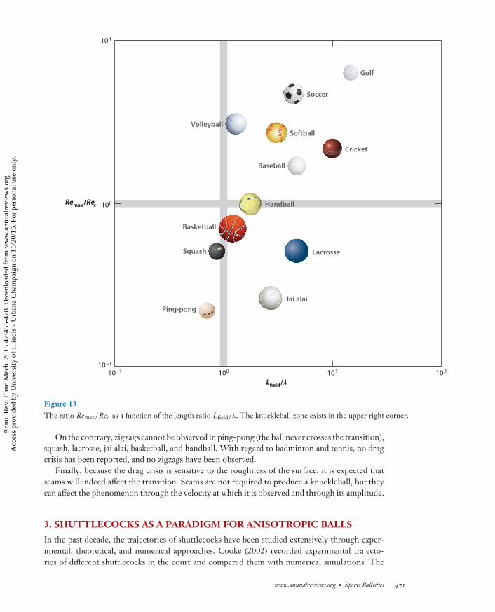
A poor man’s approach of the knuckleball is as follows: Because Figure 12b reveals that the liftcoefficient is very small except in the transition, we imagine that CLm = 0 outside the transitionand CLm = CL0 = 0.2 in the transition (values extracted from Figure 12b). With such a simplifiedmodel, Equation 17 predicts that the size of the zigzag is infinite outside the transition (and thusnot observed). In the transition, it can be observed if the distance of observation is larger than λ. Insports, the largest value of the distance of observation is the size of the field, Lfield. Table 2 presentsλ for different sports and compares it to Lfield. It also presents the critical Reynolds number, Rec, forthe different sports and compares it to the maximal value of the Reynolds number, Remax, calculatedusing Umax in Table 1. Figure 13 presents the ratio Remax/Rec as a function of the length ratioLfield/λ. In this figure, the knuckleball domain is the upper right area. Indeed, from the argumentjust developed, the ball must cross the drag crisis. Because the ball decelerates during flight, itsmaximal Reynolds number must be larger than the critical Reynolds number (Remax/Rec ≥ 1).Moreover, to be observed, the zigzag must be smaller than the sports field (Lfield/λ ≥ 1). Thoseconditions are satisfied for volleyball, baseball, softball, cricket, soccer, and golf.

The surprise here is perhaps to find golf in this category. To our knowledge, knuckleballs havenot been reported in golf, but considering the efforts dedicated by companies such as Polara toachieve straight paths, we believe that zigzags exist in golf and can be observed.

470 Clanet

Ann

u. R

ev. F

luid

Mec

h. 2

015.

47:4

55-4

78. D

ownl

oade

d fr

om w

ww

.ann

ualr

evie

ws.

org

Acc

ess

prov

ided

by

Uni

vers

ity o

f Il

linoi

s -

Urb

ana

Cha

mpa

ign

on 1

1/20

/15.

For

per

sona

l use

onl

y.

FL47CH19-Clanet ARI 18 November 2014 13:26

10 –1 100 101

10 1

100

10 –1

102

Remax/Rec

Lfield/λ

Ping-pong

Soccer

Golf

Cricket

Squash

Handball

Jai alai

Volleyball

Softball

Baseball

Basketball

Lacrosse

Figure 13The ratio Remax/Rec as a function of the length ratio Lfield/λ. The knuckleball zone exists in the upper right corner.

On the contrary, zigzags cannot be observed in ping-pong (the ball never crosses the transition),squash, lacrosse, jai alai, basketball, and handball. With regard to badminton and tennis, no dragcrisis has been reported, and no zigzags have been observed.

Finally, because the drag crisis is sensitive to the roughness of the surface, it is expected thatseams will indeed affect the transition. Seams are not required to produce a knuckleball, but theycan affect the phenomenon through the velocity at which it is observed and through its amplitude.

3. SHUTTLECOCKS AS A PARADIGM FOR ANISOTROPIC BALLS

In the past decade, the trajectories of shuttlecocks have been studied extensively through exper-imental, theoretical, and numerical approaches. Cooke (2002) recorded experimental trajecto-ries of different shuttlecocks in the court and compared them with numerical simulations. The

www.annualreviews.org • Sports Ballistics 471

Ann

u. R

ev. F

luid

Mec

h. 2

015.

47:4

55-4

78. D

ownl

oade

d fr

om w

ww

.ann

ualr

evie

ws.

org

Acc

ess

prov

ided

by

Uni

vers

ity o

f Il

linoi

s -

Urb

ana

Cha

mpa

ign

on 1

1/20

/15.

For

per

sona

l use

onl

y.

FL47CH19-Clanet ARI 18 November 2014 13:26

U

UG

B

C

(MB , S)

(MC , s)FD

FD

50 cm

a

b

φ

φ l

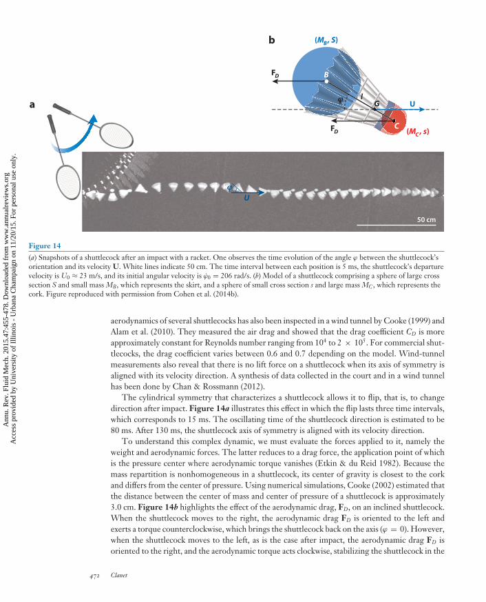
Figure 14(a) Snapshots of a shuttlecock after an impact with a racket. One observes the time evolution of the angle ϕ between the shuttlecock’sorientation and its velocity U. White lines indicate 50 cm. The time interval between each position is 5 ms, the shuttlecock’s departurevelocity is U0 ≈ 23 m/s, and its initial angular velocity is ϕ0 = 206 rad/s. (b) Model of a shuttlecock comprising a sphere of large crosssection S and small mass MB, which represents the skirt, and a sphere of small cross section s and large mass MC , which represents thecork. Figure reproduced with permission from Cohen et al. (2014b).

aerodynamics of several shuttlecocks has also been inspected in a wind tunnel by Cooke (1999) andAlam et al. (2010). They measured the air drag and showed that the drag coefficient CD is moreapproximately constant for Reynolds number ranging from 104 to 2 × 105. For commercial shut-tlecocks, the drag coefficient varies between 0.6 and 0.7 depending on the model. Wind-tunnelmeasurements also reveal that there is no lift force on a shuttlecock when its axis of symmetry isaligned with its velocity direction. A synthesis of data collected in the court and in a wind tunnelhas been done by Chan & Rossmann (2012).

The cylindrical symmetry that characterizes a shuttlecock allows it to flip, that is, to changedirection after impact. Figure 14a illustrates this effect in which the flip lasts three time intervals,which corresponds to 15 ms. The oscillating time of the shuttlecock direction is estimated to be80 ms. After 130 ms, the shuttlecock axis of symmetry is aligned with its velocity direction.

To understand this complex dynamic, we must evaluate the forces applied to it, namely theweight and aerodynamic forces. The latter reduces to a drag force, the application point of whichis the pressure center where aerodynamic torque vanishes (Etkin & du Reid 1982). Because themass repartition is nonhomogeneous in a shuttlecock, its center of gravity is closest to the corkand differs from the center of pressure. Using numerical simulations, Cooke (2002) estimated thatthe distance between the center of mass and center of pressure of a shuttlecock is approximately3.0 cm. Figure 14b highlights the effect of the aerodynamic drag, FD, on an inclined shuttlecock.When the shuttlecock moves to the right, the aerodynamic drag FD is oriented to the left andexerts a torque counterclockwise, which brings the shuttlecock back on the axis (ϕ = 0). However,when the shuttlecock moves to the left, as is the case after impact, the aerodynamic drag FD isoriented to the right, and the aerodynamic torque acts clockwise, stabilizing the shuttlecock in the

472 Clanet

Ann

u. R

ev. F

luid

Mec

h. 2

015.

47:4

55-4

78. D

ownl

oade

d fr

om w

ww

.ann

ualr

evie

ws.

org

Acc

ess

prov

ided

by

Uni

vers

ity o

f Il

linoi

s -

Urb

ana

Cha

mpa

ign

on 1

1/20

/15.

For

per

sona

l use

onl

y.

FL47CH19-Clanet ARI 18 November 2014 13:26

α

β0

β

y = −H

x

ba ccU0

U

n

y

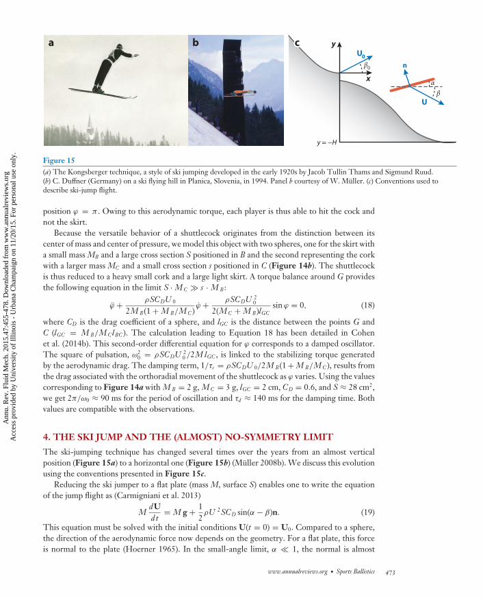
Figure 15(a) The Kongsberger technique, a style of ski jumping developed in the early 1920s by Jacob Tullin Thams and Sigmund Ruud.(b) C. Duffner (Germany) on a ski flying hill in Planica, Slovenia, in 1994. Panel b courtesy of W. Muller. (c) Conventions used todescribe ski-jump flight.

position ϕ = π . Owing to this aerodynamic torque, each player is thus able to hit the cock andnot the skirt.

Because the versatile behavior of a shuttlecock originates from the distinction between itscenter of mass and center of pressure, we model this object with two spheres, one for the skirt witha small mass MB and a large cross section S positioned in B and the second representing the corkwith a larger mass MC and a small cross section s positioned in C (Figure 14b). The shuttlecockis thus reduced to a heavy small cork and a large light skirt. A torque balance around G providesthe following equation in the limit S · M C � s · M B :

ϕ + ρSCDU 0

2M B (1 + M B/M C )ϕ + ρSCDU 2

0

2(M C + M B )lGCsin ϕ = 0, (18)

where CD is the drag coefficient of a sphere, and lGC is the distance between the points G andC (lGC = M B/M ClBC ). The calculation leading to Equation 18 has been detailed in Cohenet al. (2014b). This second-order differential equation for ϕ corresponds to a damped oscillator.The square of pulsation, ω2

0 = ρSCDU 20 /2M lGC , is linked to the stabilizing torque generated

by the aerodynamic drag. The damping term, 1/τs = ρSCDU 0/2M B (1 + M B/M C ), results fromthe drag associated with the orthoradial movement of the shuttlecock as ϕ varies. Using the valuescorresponding to Figure 14a with M B = 2 g, M C = 3 g, lGC = 2 cm, CD = 0.6, and S ≈ 28 cm2,we get 2π/ω0 ≈ 90 ms for the period of oscillation and τd ≈ 140 ms for the damping time. Bothvalues are compatible with the observations.

4. THE SKI JUMP AND THE (ALMOST) NO-SYMMETRY LIMIT

The ski-jumping technique has changed several times over the years from an almost verticalposition (Figure 15a) to a horizontal one (Figure 15b) (Muller 2008b). We discuss this evolutionusing the conventions presented in Figure 15c.

Reducing the ski jumper to a flat plate (mass M, surface S) enables one to write the equationof the jump flight as (Carmigniani et al. 2013)

MdUdt

= M g + 12ρU 2SCD sin(α − β)n. (19)

This equation must be solved with the initial conditions U(t = 0) = U0. Compared to a sphere,the direction of the aerodynamic force now depends on the geometry. For a flat plate, this forceis normal to the plate (Hoerner 1965). In the small-angle limit, α � 1, the normal is almost

www.annualreviews.org • Sports Ballistics 473

Ann

u. R

ev. F

luid

Mec

h. 2

015.

47:4

55-4

78. D

ownl

oade

d fr

om w

ww

.ann

ualr

evie

ws.

org

Acc

ess

prov

ided

by

Uni

vers

ity o

f Il

linoi

s -

Urb

ana

Cha

mpa

ign

on 1

1/20

/15.

For

per

sona

l use

onl

y.

FL47CH19-Clanet ARI 18 November 2014 13:26

aligned with the vertical (n · ex ≈ 0), and Equation 19 reduces in the ex direction to dU x/dt = 0,from which we obviously get x = U 0 cos β0t. Along the ey direction, Equation 19 reduces todU y/dt = −g − ρSCD cos αU U y/2M . Following the studies of Muller et al. (1995) and Muller(2008a), it appears that the velocity U weakly changes between takeoff and landing, maintaininga value close to 30 m/s. The condition U ≈ U 0 allows one to integrate the equation and get theapproximate trajectory:

gyU 2

0= − gx

U 20

1Dr cos α cos β0

+ 1 + Dr cos α sin β0

(Dr cosα)2

[1 − e

− gxU 2

0

Dr cosαcos β0

], (20)

where Dr = ρU 20 SCD/2M g is the drag to weight ratio. In the limit of small drag (Dr � 1), the

trajectory in Equation 20 reduces to the parabolic flight in Equation 5. In the opposite limit of aperfect flyer (Dr � 1), the trajectory in Equation 20 allows one to predict the jump length at afixed location y = −H:

x(y = −H ) ≈ H · Dr cos α · cos β0. (21)

This expression reveals that the length of the jump is maximized for large values of Dr andfor cos α = 1 and cos β0 = 1. For athletes, one way to increase Dr is to decrease their mass(limM →0 Dr = ∞). This effect did have major consequences for ski jumpers in the sense that somebecame anorexic (Schmolzer & Muller 2002). The condition cos α = 1 allows us to understandthe horizontal position observed in Figure 15b. Finally, the condition cos β0 = 1 also allows us tounderstand the large effort by athletes to increase their vertical velocity at takeoff (Virmavirta et al.2009). Indeed, the in-run track makes a −10◦ angle with the horizontal direction. To get close tothe condition β0 = 0, an athlete must reach a vertical velocity of U y0 = U 0 sin(10) ≈ 5.2 m/s.This value is compatible with measurements performed at takeoff by Virmavirta et al. (2009) andMuller (2013). The model just discussed is obviously too basic to account for the complexity of thewhole phenomenon, and more detailed approaches can be found in Schmolzer & Muller (2005).

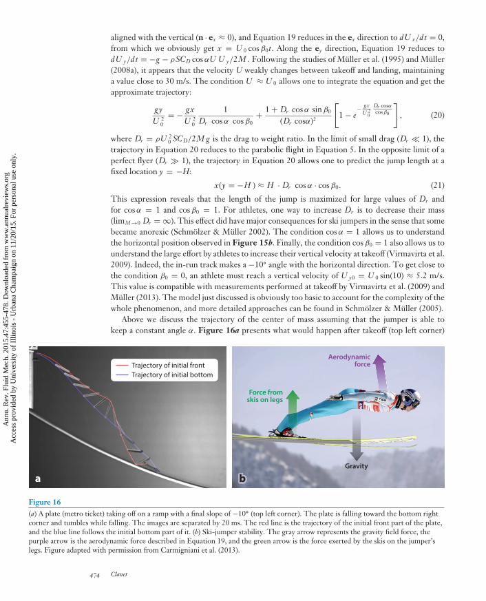
Above we discuss the trajectory of the center of mass assuming that the jumper is able tokeep a constant angle α. Figure 16a presents what would happen after takeoff (top left corner)

a b

Trajectory of initial front

Trajectory of initial bottom

Gravity

Aerodynamicforce

Force fromskis on legs

Figure 16(a) A plate (metro ticket) taking off on a ramp with a final slope of −10◦ (top left corner). The plate is falling toward the bottom rightcorner and tumbles while falling. The images are separated by 20 ms. The red line is the trajectory of the initial front part of the plate,and the blue line follows the initial bottom part of it. (b) Ski-jumper stability. The gray arrow represents the gravity field force, thepurple arrow is the aerodynamic force described in Equation 19, and the green arrow is the force exerted by the skis on the jumper’slegs. Figure adapted with permission from Carmigniani et al. (2013).

474 Clanet

Ann

u. R

ev. F

luid

Mec

h. 2

015.

47:4

55-4

78. D

ownl

oade

d fr

om w

ww

.ann

ualr

evie

ws.

org

Acc

ess

prov

ided

by

Uni

vers

ity o

f Il

linoi

s -

Urb

ana

Cha

mpa

ign

on 1

1/20

/15.

For

per

sona

l use

onl

y.

FL47CH19-Clanet ARI 18 November 2014 13:26

if the jumper were really behaving as a flat plate. Because the aerodynamic force applies at theaerodynamic center, which is close to the leading edge for a plate, the aerodynamic force exertsa torque on the plate that makes it rotate counterclockwise. To avoid this tumbling instability(Mahadevanand et al. 1996, Andersen et al. 2005), the ski jumper balances the aerodynamic forceacting on his or her body by the aerodynamic force acting on the skis (Figure 16b). Althoughnot presented in the figure, the arms also help the jumper to achieve stability (Marques-Bruna &Grimshaw 2009a,b).

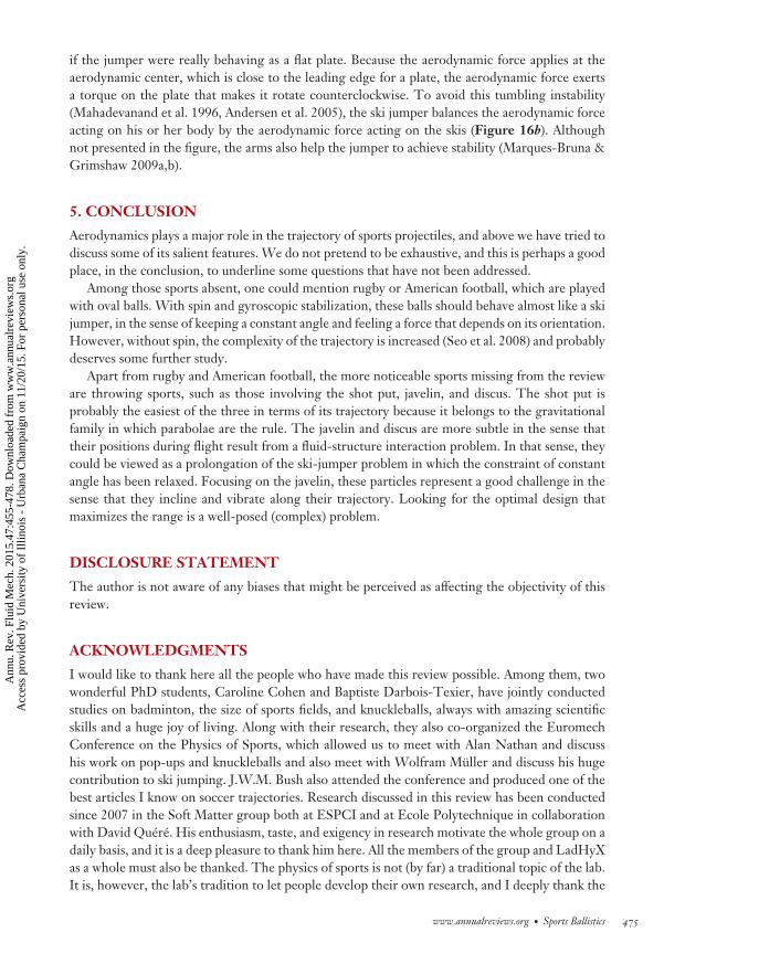
5. CONCLUSION

Aerodynamics plays a major role in the trajectory of sports projectiles, and above we have tried todiscuss some of its salient features. We do not pretend to be exhaustive, and this is perhaps a goodplace, in the conclusion, to underline some questions that have not been addressed.

Among those sports absent, one could mention rugby or American football, which are playedwith oval balls. With spin and gyroscopic stabilization, these balls should behave almost like a skijumper, in the sense of keeping a constant angle and feeling a force that depends on its orientation.However, without spin, the complexity of the trajectory is increased (Seo et al. 2008) and probablydeserves some further study.

Apart from rugby and American football, the more noticeable sports missing from the revieware throwing sports, such as those involving the shot put, javelin, and discus. The shot put isprobably the easiest of the three in terms of its trajectory because it belongs to the gravitationalfamily in which parabolae are the rule. The javelin and discus are more subtle in the sense thattheir positions during flight result from a fluid-structure interaction problem. In that sense, theycould be viewed as a prolongation of the ski-jumper problem in which the constraint of constantangle has been relaxed. Focusing on the javelin, these particles represent a good challenge in thesense that they incline and vibrate along their trajectory. Looking for the optimal design thatmaximizes the range is a well-posed (complex) problem.

DISCLOSURE STATEMENT

The author is not aware of any biases that might be perceived as affecting the objectivity of thisreview.

ACKNOWLEDGMENTS

I would like to thank here all the people who have made this review possible. Among them, twowonderful PhD students, Caroline Cohen and Baptiste Darbois-Texier, have jointly conductedstudies on badminton, the size of sports fields, and knuckleballs, always with amazing scientificskills and a huge joy of living. Along with their research, they also co-organized the EuromechConference on the Physics of Sports, which allowed us to meet with Alan Nathan and discusshis work on pop-ups and knuckleballs and also meet with Wolfram Muller and discuss his hugecontribution to ski jumping. J.W.M. Bush also attended the conference and produced one of thebest articles I know on soccer trajectories. Research discussed in this review has been conductedsince 2007 in the Soft Matter group both at ESPCI and at Ecole Polytechnique in collaborationwith David Quere. His enthusiasm, taste, and exigency in research motivate the whole group on adaily basis, and it is a deep pleasure to thank him here. All the members of the group and LadHyXas a whole must also be thanked. The physics of sports is not (by far) a traditional topic of the lab.It is, however, the lab’s tradition to let people develop their own research, and I deeply thank the

www.annualreviews.org • Sports Ballistics 475

Ann

u. R

ev. F

luid

Mec

h. 2

015.

47:4

55-4

78. D

ownl

oade

d fr

om w

ww

.ann

ualr

evie

ws.

org

Acc

ess

prov

ided

by

Uni

vers

ity o

f Il

linoi

s -

Urb

ana

Cha

mpa

ign

on 1

1/20

/15.

For

per

sona

l use

onl

y.

FL47CH19-Clanet ARI 18 November 2014 13:26

whole lab for respecting this tradition. Outside the lab, I sincerely thank E. Reyssat, M. Rabaud,P. Gondret, J.P. Hulin, M. Fermigier, and E. Guyon for their attentive reading of the originalversion of the article and their constructive comments. Finally, this review would not have existedwithout Elisabeth Guazzelli, who proposed it to me two years ago. May all of them find in thesefew lines the expression of my sincere gratitude.

LITERATURE CITED

Alam F, Chowdhury H, Theppadungporn C, Subic A. 2010. Measurements of aerodynamic properties ofbadminton shuttlecocks. Procedia Eng. 2:2487–92

Alam F, Ho H, Smith L, Subic A, Chowdhury H, Kumar A. 2012. A study of baseball and softball aerodynamics.Procedia Eng. 34:86–91

Andersen A, Pesavento U, Wang J. 2005. Analysis of transitions between fluttering, tumbling and steadydescent of falling cards. J. Fluid Mech. 541:91–104

Asai T, Kamemoto K. 2011. Flow structure of knuckling effect in footballs. J. Fluids Struct. 27:727–33Asai T, Seo K, Kobayashi O, Sakashita R. 2007. Fundamental aerodynamics of the soccer ball. Sports Eng.

10:101–10Barber S, Chin S, Carre M. 2009. Sports ball aerodynamics: a numerical study of the erratic motion of soccer

balls. Comput. Fluids 38:1091–100Bush J. 2013. The aerodynamics of the beautiful game. See Clanet 2013, pp. 171–92Carmigniani R, Cao X, Savourey S, Martinier C, Nuytten S, et al. 2013. Ski jump flight. See Clanet 2013,

pp. 286–301Chan C, Rossmann J. 2012. Badminton shuttlecock aerodynamics: synthesizing experiment and theory. Sports

Eng. 15:61–71Cho A. 2004. Engineering of sport. Science 306:42–43Chudinov P. 2010. Approximate formula for the vertical asymptote of projectile motion in midair. Int. J. Math.

Educ. Sci. Technol. 41:92–98Clanet C, ed. 2013. Sports Physics. Palaiseau, Fr.: Ed. Ecole Polytech.Cohen C, Darbois-Texier B, Dupeux G, Brunel E, Quere D, Clanet C. 2014a. The aerodynamical wall. Proc.

R. Soc. Lond. A 470:20130497Cohen C, Darbois-Texier B, Quere D, Clanet C. 2014b. Physics of badminton. New J. Phys. In pressCooke A. 1999. Shuttlecock aerodynamics. Sports Eng. 2:85–96Cooke A. 2002. Computer simulation of shuttlecock trajectories. Sport Eng. 5:93–105Cottey R. 2002. The modelling of spin generation with particular emphasis on racket ball games. PhD Thesis,

Loughborough Univ.Darbois-Texier B. 2013. Tartaglia, zigzag and flips: les particules denses a haut Reynolds. PhD Thesis, Univ. Paris

DiderotDarbois-Texier B, Cohen C, Dupeux G, Quere D, Clanet C. 2014. On the size of sports fields. New J. Phys.

16:033039Darbois-Texier B, Cohen C, Quere D, Clanet C. 2013. Knuckleballs. See Clanet 2013, pp. 199–212de Mestre N. 1990. The Mathematics of Projectiles in Sport. Cambridge, UK: Cambridge Univ. PressDepra P, Brenzikofer R, Goes M, Barros R. 1998. Fluid mechanics analysis in volleyball services. 16 Int. Symp.

Biomech. Sports. Int. Soc. Biomech. Sports. https://ojs.ub.uni-konstanz.de/cpa/article/view/1602Drake S. 1973. Galileo’s experimental confirmation of horizontal inertia: unpublished manuscripts. Isis 64:291–

305Dupeux G, Cohen C, Goff AL, Quere D, Clanet C. 2011. Football curves. J. Fluids Struct. 27:659–67Dupeux G, Goff AL, Quere D, Clanet C. 2010. The spinning ball spiral. New J. Phys. 12:093004eFastball.com. 2011. Bat speed, batted ball speed (exit speed) in MPH by age group. http://www.efastball.

com/hitting/average-bat-speed-exit-speed-by-age-group/Erlichson H. 1983. Maximum projectile range with drag and lift, with particular application to golf. Am. J.

Phys. 51:357–62

476 Clanet

Ann

u. R

ev. F

luid

Mec

h. 2

015.

47:4

55-4

78. D

ownl

oade

d fr

om w

ww

.ann

ualr

evie

ws.

org

Acc

ess

prov

ided

by

Uni

vers

ity o

f Il

linoi

s -

Urb

ana

Cha

mpa

ign

on 1

1/20

/15.

For

per

sona

l use

onl

y.

FL47CH19-Clanet ARI 18 November 2014 13:26

Ern P, Risso F, Fabre D, Magnaudet J. 2012. Wake-induced oscillatory paths of bodies freely rising or fallingin fluids. Annu. Rev. Fluid Mech. 44:97–121

Etkin B, du Reid L. 1982. Dynamics of Flight: Stability and Control. New York: WileyFrohlich C. 2011. Resource letter PS-2: physics of sports. Am. J. Phys. 79:565–74Galilei G. 1638. Dialogues Concerning Two New Sciences. Leiden: L. ElzevierGillmeister H. 1998. Tennis: A Cultural History. New York: New York Univ. PressGorostiaga E, Granados C, Ibanez J, Izquierdo M. 2005. Differences in physical fitness and throwing velocity

among elite and amateur male handball players. Int. J. Sports Med. 26:225–32Greenwald R, Penna L, Crisco J. 2001. Differences in batted ball speed with wood and aluminum baseball

bats: a batting cage study. J. Appl. Biomech. 17:241–52Hayrinen M, Lahtinen P, Mikkola T, Honkanen P, Paananen A, Blomqvist M. 2007. Serve speed analysis in

men’s volleyball. Presented at Science for Success II, Jyvaskyla, Finl.Higuchi H, Kiura T. 2012. Aerodynamics of knuckleball: flow-structure interaction problem on a pitched

baseball without spin. J. Fluids Struct. 32:65–77Hoerner SF. 1965. Fluid-Dynamic Drag. Bricktown, NJ: Hoerner Fluid Dyn.Hong S, Chung C, Nakayama M, Asai T. 2010. Unsteady aerodynamic force on a knuckleball in soccer.

Procedia Eng. 2:2455–60Horowitz M, Williamson CHK. 2010. The effect of Reynolds number on the dynamics and wakes of freely

rising and falling spheres. J. Fluid Mech. 651:251–94Huston R, Cesar A. 2003. Basketball shooting strategies: the free throw, direct shot and layup. Sports Eng.

6:49–64Keller J. 1974. Optimal velocity in a race. Am. Math. Mon. 81:474–80Lamb H. 1914. Dynamics. Cambridge, UK: Cambridge Univ. PressMacKenzie S, Kortegaard K, LeVangie M, Barro B. 2012. Evaluation of two methods of the jump float serve

in volleyball. J. Appl. Biomech. 28:579–86Mahadevanand L, Ryu W, Adt S. 1996. Tumbling cards. Phys. Fluids 11:1–3Marques-Bruna P, Grimshaw P. 2009a. Mechanics of flight in ski jumping: aerodynamic stability in pitch.

Sports Technol. 2:24–31Marques-Bruna P, Grimshaw P. 2009b. Mechanics of flight in ski jumping: aerodynamic stability in roll and

yaw. Sports Technol. 2:111–20McBeath MK, Nathan AM, Bahill AT, Baldwin DG. 2008. Paradoxical pop-ups: Why are they difficult to

catch? Am. J. Phys. 76:723–29Mehta D. 1985. Aerodynamics of sports balls. Annu. Rev. Fluid Mech. 17:151–89Mehta R. 2008. Sports ball aerodynamics. In Sport Aerodynamics, ed. H Norstrud, pp. 229–331. New York:

SpringerMehta R, Alam F, Subic A. 2008. Aerodynamics of tennis balls: a review. Sports Technol. 1:1–10Mehta R, Pallis J. 2001. Sports ball aerodynamics: effects of velocity, spin and surface roughness. In Materials

and Science in Sports, ed. S Froes, S Haake, pp. 185–97. Warrendale, PA: TMSMuller W. 2008a. Computer simulation of ski jumping based on wind tunnel data. Sport Aerodyn. 506:161–82Muller W. 2008b. Performance factors in ski jumping. Sport Aerodyn. 506:139–60Muller W. 2013. Physics of ski jumping. See Clanet 2013, pp. 271–86Muller W, Platzer D, Schmolzer B. 1995. Scientific approach to ski safety. Nature 375:455Nathan AM. 2003. Characterizing the performance of baseball bats. Am. J. Phys. 71:134–43Nathan AM. 2008. The effect of spin on the flight of a baseball. Am. J. Phys. 76:119–24Nathan AM. 2012. Analysis of knuckleball trajectories. Procedia Eng. 34:116–21Newton I. 1671. New theory about light and colors. Philos. Trans. 6:3075–87Norman A, McKeon B. 2011. Unsteady force measurements in sphere flow from subcritical to supercritical

Reynolds numbers. Exp. Fluids 51:1439–53Rayleigh L. 1877. On the irregular flight of a tennis ball. Messenger Math. 7:14–16Reep C, Benjamin B. 1968. Skill and chance in association football. J. R. Stat. Soc. A 131:581–85RIA Novosti. 2013. Malaysian badminton star breaks smash speed record. RIA Novosti, Aug. 23. http://en.ria.

ru/sports/20130823/182930446.html

www.annualreviews.org • Sports Ballistics 477

Ann

u. R

ev. F

luid

Mec

h. 2

015.

47:4

55-4

78. D

ownl

oade

d fr

om w

ww

.ann

ualr

evie

ws.

org

Acc

ess

prov

ided

by

Uni

vers

ity o

f Il

linoi

s -

Urb

ana

Cha

mpa

ign

on 1

1/20

/15.

For

per

sona

l use

onl

y.

FL47CH19-Clanet ARI 18 November 2014 13:26

Russell DA. 2008. Explaining the 98-mph BBS standard for ASA softball. http://www.acs.psu.edu/drussell/bats/bbs-asa.html

Schmolzer B, Muller W. 2002. The importance of being light: aerodynamic forces and weight in ski jumping.J. Biomech. 35:1059–69

Schmolzer B, Muller W. 2005. Individual flight styles in ski jumping: results obtained during Olympic Gamescompetitions. J. Biomech. 38:1055–65

Seo K, Kobayashi O, Murakami M. 2008. The fluctuating flight trajectory of a non-spinning punted ball inrugby. Eng. Sport 7:329–36

Sheppard D. 2013. Tracking R.A. Dickey’s knuckleball. FanGraphs, June 18. http://www.fangraphs.com/blogs/tracking-r-a-dickeys-knuckleball/

Tartaglia N. 1537. Nova Scientia. Venice: Stefano dei Nicolini da SabbioTruscott TT, Techet AH. 2009. Water entry of spinning spheres. J. Fluid Mech. 625:135–65Turberville J. 2003. Table tennis ball speed. http://www.jayandwanda.com/tt/speed.htmlVirmavirta M, Isolehto J, Komi P, Schwameder H, Pigozzi F, Massazza G. 2009. Take-off analysis of the

Olympic ski jumping competition (HS-106m). J. Biomech. 42:1095–101Volleywood. 2012. Matey & Santos’ lightning spikes. Volleywood, May 8. http://www.volleywood.net/

volleyball-related-news/volleyball-news-north-america/kaziyski-santos-lightning-spikes/Willmarth W, Enlow RL. 1969. Aerodynamic lift and moment fluctuations of a sphere. J. Fluid Mech. 36:417–

32

478 Clanet

Ann

u. R

ev. F

luid

Mec

h. 2

015.

47:4

55-4

78. D

ownl

oade

d fr

om w

ww

.ann

ualr

evie

ws.

org

Acc

ess

prov

ided

by

Uni

vers

ity o

f Il

linoi

s -

Urb

ana

Cha

mpa

ign

on 1

1/20

/15.

For

per

sona

l use

onl

y.

FL47-FrontMatter ARI 22 November 2014 11:57

Annual Review ofFluid Mechanics

Volume 47, 2015Contents

Fluid Mechanics in Sommerfeld’s SchoolMichael Eckert � � � � � � � � � � � � � � � � � � � � � � � � � � � � � � � � � � � � � � � � � � � � � � � � � � � � � � � � � � � � � � � � � � � � � � � � � � � � � � � � � � 1

Discrete Element Method Simulations for Complex Granular FlowsYu Guo and Jennifer Sinclair Curtis � � � � � � � � � � � � � � � � � � � � � � � � � � � � � � � � � � � � � � � � � � � � � � � � � � � � � � � � �21

Modeling the Rheology of Polymer Melts and SolutionsR.G. Larson and Priyanka S. Desai � � � � � � � � � � � � � � � � � � � � � � � � � � � � � � � � � � � � � � � � � � � � � � � � � � � � � � � � � �47

Liquid Transfer in Printing Processes: Liquid Bridges with MovingContact LinesSatish Kumar � � � � � � � � � � � � � � � � � � � � � � � � � � � � � � � � � � � � � � � � � � � � � � � � � � � � � � � � � � � � � � � � � � � � � � � � � � � � � � � � � �67

Dissipation in Turbulent FlowsJ. Christos Vassilicos � � � � � � � � � � � � � � � � � � � � � � � � � � � � � � � � � � � � � � � � � � � � � � � � � � � � � � � � � � � � � � � � � � � � � � � � � � �95

Floating Versus SinkingDominic Vella � � � � � � � � � � � � � � � � � � � � � � � � � � � � � � � � � � � � � � � � � � � � � � � � � � � � � � � � � � � � � � � � � � � � � � � � � � � � � � � � 115

Langrangian Coherent StructuresGeorge Haller � � � � � � � � � � � � � � � � � � � � � � � � � � � � � � � � � � � � � � � � � � � � � � � � � � � � � � � � � � � � � � � � � � � � � � � � � � � � � � � � 137

Flows Driven by Libration, Precession, and TidesMichael Le Bars, David Cebron, and Patrice Le Gal � � � � � � � � � � � � � � � � � � � � � � � � � � � � � � � � � � � � � 163

Fountains in Industry and NatureG.R. Hunt and H.C. Burridge � � � � � � � � � � � � � � � � � � � � � � � � � � � � � � � � � � � � � � � � � � � � � � � � � � � � � � � � � � � � � 195

Acoustic Remote SensingDavid R. Dowling and Karim G. Sabra � � � � � � � � � � � � � � � � � � � � � � � � � � � � � � � � � � � � � � � � � � � � � � � � � � � 221

Coalescence of DropsH. Pirouz Kavehpour � � � � � � � � � � � � � � � � � � � � � � � � � � � � � � � � � � � � � � � � � � � � � � � � � � � � � � � � � � � � � � � � � � � � � � � 245

Pilot-Wave HydrodynamicsJohn W.M. Bush � � � � � � � � � � � � � � � � � � � � � � � � � � � � � � � � � � � � � � � � � � � � � � � � � � � � � � � � � � � � � � � � � � � � � � � � � � � � 269

Ignition, Liftoff, and Extinction of Gaseous Diffusion FlamesAmable Linan, Marcos Vera, and Antonio L. Sanchez � � � � � � � � � � � � � � � � � � � � � � � � � � � � � � � � � � � � 293

The Clinical Assessment of Intraventricular FlowsJavier Bermejo, Pablo Martınez-Legazpi, and Juan C. del Alamo � � � � � � � � � � � � � � � � � � � � � � 315

v

Ann

u. R

ev. F

luid

Mec

h. 2

015.

47:4

55-4

78. D

ownl

oade

d fr

om w

ww

.ann

ualr

evie

ws.

org

Acc

ess

prov

ided

by

Uni

vers

ity o

f Il

linoi

s -

Urb

ana

Cha

mpa

ign

on 1

1/20

/15.

For

per

sona

l use

onl

y.

FL47-FrontMatter ARI 22 November 2014 11:57

Green Algae as Model Organisms for Biological Fluid DynamicsRaymond E. Goldstein � � � � � � � � � � � � � � � � � � � � � � � � � � � � � � � � � � � � � � � � � � � � � � � � � � � � � � � � � � � � � � � � � � � � � � � 343

Fluid Mechanics of Blood Clot FormationAaron L. Fogelson and Keith B. Neeves � � � � � � � � � � � � � � � � � � � � � � � � � � � � � � � � � � � � � � � � � � � � � � � � � � � � 377

Generation of Microbubbles with Applications to Industry and MedicineJavier Rodrıguez-Rodrıguez, Alejandro Sevilla, Carlos Martınez-Bazan,

and Jose Manuel Gordillo � � � � � � � � � � � � � � � � � � � � � � � � � � � � � � � � � � � � � � � � � � � � � � � � � � � � � � � � � � � � � � � � 405

Beneath Our Feet: Strategies for Locomotion in Granular MediaA.E. Hosoi and Daniel I. Goldman � � � � � � � � � � � � � � � � � � � � � � � � � � � � � � � � � � � � � � � � � � � � � � � � � � � � � � � � � 431

Sports BallisticsChristophe Clanet � � � � � � � � � � � � � � � � � � � � � � � � � � � � � � � � � � � � � � � � � � � � � � � � � � � � � � � � � � � � � � � � � � � � � � � � � � � � 455

Dynamic Stall in Pitching Airfoils: Aerodynamic Damping andCompressibility EffectsThomas C. Corke and Flint O. Thomas � � � � � � � � � � � � � � � � � � � � � � � � � � � � � � � � � � � � � � � � � � � � � � � � � � � � 479

Ocean SprayFabrice Veron � � � � � � � � � � � � � � � � � � � � � � � � � � � � � � � � � � � � � � � � � � � � � � � � � � � � � � � � � � � � � � � � � � � � � � � � � � � � � � � � 507

Stability of Constrained Capillary SurfacesJ.B. Bostwick and P.H. Steen � � � � � � � � � � � � � � � � � � � � � � � � � � � � � � � � � � � � � � � � � � � � � � � � � � � � � � � � � � � � � � � 539

Mixing and Transport in Coastal River PlumesAlexander R. Horner-Devine, Robert D. Hetland, and Daniel G. MacDonald � � � � � � � � � 569

Indexes

Cumulative Index of Contributing Authors, Volumes 1–47 � � � � � � � � � � � � � � � � � � � � � � � � � � � � 595

Cumulative Index of Article Titles, Volumes 1–47 � � � � � � � � � � � � � � � � � � � � � � � � � � � � � � � � � � � � � � � 605

Errata

An online log of corrections to Annual Review of Fluid Mechanics articles may be foundat http://www.annualreviews.org/errata/fluid

vi Contents

Ann

u. R

ev. F

luid

Mec

h. 2

015.

47:4

55-4

78. D

ownl

oade

d fr

om w

ww

.ann

ualr

evie

ws.

org

Acc

ess

prov

ided

by

Uni

vers

ity o

f Il

linoi

s -

Urb

ana

Cha

mpa

ign

on 1

1/20

/15.

For

per

sona

l use

onl

y.