Martin Glanzer, BSc

SPREAD OPTION VALUATION IN

ORNSTEIN-UHLENBECK TYPE STOCHASTIC

VOLATILITY MODELS

MASTERARBEIT

zur Erlangung des akademischen Grades

Diplom-Ingenieur

Masterstudium Finanz- und Versicherungsmathematik

eingereicht an der

Technischen Universität Graz

Betreuer:O. Univ.-Prof. Dr. phil. Robert TICHY

Assoc. Prof. Carlo SGARRA, Ph.D.

Institut für Analysis und Computational Number Theory (Math A)Department of Mathematics - Politecnico di Milano

Graz, Mai 2014

EIDESSTATTLICHE ERKLÄRUNG

AFFIDAVIT

Ich erkläre an Eides statt, dass ich die vorliegende Arbeit selbstständig verfasst, an-dere als die angegebenen Quellen/Hilfsmittel nicht benutzt, und die den benutztenQuellen wörtlich und inhaltlich entnommenen Stellen als solche kenntlich gemachthabe. Das in TUGRAZonline hochgeladene Textdokument ist mit der vorliegendenMasterarbeit identisch.

I declare that I have authored this thesis independently, that I have not used otherthan the declared sources/resources, and that I have explicitly indicated all materialwhich has been quoted either literally or by content from the sources used. The textdocument uploaded to TUGRAZonline is identical to the present master’s thesis.

Datum/Date Unterschrift/Signature

Abstract

This thesis examines the valuation problem for Spread Options in market models,where the volatility process is of Ornstein-Uhlenbeck type. An appropriate formu-lation of these models in a multidimensional setting requires a matrix subordinationapproach, i.e., the Ornstein-Uhlenbeck process is driven by a matrix-valued Lévyprocess, whose increments only take values in the cone of positive semidefinite sym-metric matrices. Such models have gained some popularity in the modelling ofequity markets and, more recently, in commodity and energy markets. The liter-ature about pricing methods for Spread Options in non-Gaussian setups is sparse;however, in models where the joint characteristic function of the log-return processis known in closed form, some techniques based on the fast Fourier transform (FFT)are available and allow for efficient valuation.

The contribution of this thesis is the following: We compute explicit prices forSpread Options in the two-dimensional OU-Wishart model. From a computationalpoint of view, we compare the results obtained by a Monte-Carlo simulation withthose obtained by an FFT method. We investigate the FFT method in detailand implement it in two different ways in order to deal with any given contract-characteristics. Realizing the drawbacks of the particular FFT method, which arerevealed by our analyses, we discuss alternative possibilities in order to (possibly)avoid them. In particular, we comment on the Integration-Along-Cut method andtake first steps for possible applicability (future work required).

From a modelling perspective, we particularly address the issue of specifying thestationary distribution of the volatility process. Under some simplifying assump-tions, we formulate a particular specification of the general multivariate IG-OUtype stochastic volatiliy model and derive the joint characteristic function of thetwo-dimensional log-return process within our model. Moreover, we examine a firsttesting of parameter sensitivities for this special case that we consider.

i

Acknowledgements

This thesis marks the end of my student days. Therefore, I would like to take theopportunity to express my gratitude to a number of people, who supported meregarding this thesis, or accompanied me on my way during the past years.

I want to thank Dr. Markus Hofer, who initially suggested to me the interestingsubject of Ornstein-Uhlenbeck type Stochastic Volatility models, and who facilitatedmy visit to the Politecnico di Milano. I want to thank my supervisor, ProfessorRobert Tichy, for his support and cooperativeness. I particularly want to expressmy deepest gratitude to Professor Carlo Sgarra from the Politecnico di Milano, whoguided me through this thesis, always took his time for all my questions, and mademy stay in Milan such an interesting and educational time; I was incredibly luckyto have the privilege to profit from his expertise and passion for mathematics andresearch. I am thankful for the support of Assistant Professor Daniele Marazzina,who helped me regarding the numerical part of this thesis.

I am indebted to the group of students at TU Graz, who accompanied me all theyears of my studies: for all the exercise sessions we prepared together and all thepre-exam discussions. Without this support, it would have never ever been possiblefor me to proceed in the same way.

On a personal level, I want to say that I am very glad that I have always hadfriends and companions, who also shared the pleasures of life with me outside theuniversity. There are so many nice experiences and memories that will always re-main in my mind and make me smile, whenever I will think back to my student days.Special thanks to everybody, who will be part of one or more of these memories.

Finally, but most of all, I want to thank my parents; not only for their supportand for enabling me to live an exciting and pleasant student life without any sorrows,but rather for giving me a strong background and equipping me with motivationand confidence, making it a pleasure to meet the challenges of life and persistentlywork on my goals.

ii

List of Abbreviations

a.s. ..... almost surely

BM ..... Brownian motion

BDLP ..... Background Driving Lévy process

BNS ..... Barndorff-Nielsen and Shephard (model)

CI ..... confidence interval

CPP ..... Compound Poisson process

CV ..... control variate

DFT ..... Discrete Fourier transform

EMM ..... equivalent martingale measure

FFT ..... Fast Fourier transform

GBM ..... Geometric Brownian motion

GH ..... Generalized Hyperbolic (distribution)

GIG ..... Generalized inverse Gaussian (distribution)

IAC ..... Integration-Along-Cut method

IG ..... inverse Gaussian (distribution/process)

i.i.d ..... independent and identically distributed

MC ..... Monte-Carlo (simulation)

mgf ..... moment generating function

NIG ..... normal inverse Gaussian (distribution/process)

OTC ..... over-the-counter

OU ..... Ornstein-Uhlenbeck

SDE ..... stochastic differential equation

SV ..... Stochastic Volatility (models)

iii

Contents

1 Introduction 1

2 Spread Options 52.1 Pricing methods for Spread Options . . . . . . . . . . . . . . . . . . 7

2.1.1 Fourier transform methods for option pricing . . . . . . . . . 92.1.2 Using the Fast Fourier transform for option pricing: The

method of Carr and Madan . . . . . . . . . . . . . . . . . . 102.1.3 The method of Hurd and Zhou for Spread Option pricing . . 16

3 Theory of Lévy Processes and Market Modelling 233.1 Lévy Processes . . . . . . . . . . . . . . . . . . . . . . . . . . . . . 23

3.1.1 A review of general theory . . . . . . . . . . . . . . . . . . . 233.1.2 Increasing Lévy processes: Subordinators . . . . . . . . . . . 283.1.3 Selected examples of Lévy processes . . . . . . . . . . . . . . 29

3.2 Processes of Ornstein-Uhlenbeck type . . . . . . . . . . . . . . . . . 333.2.1 Gaussian Ornstein-Uhlenbeck processes . . . . . . . . . . . . 333.2.2 General Ornstein-Uhlenbeck processes . . . . . . . . . . . . 35

3.3 Market modelling . . . . . . . . . . . . . . . . . . . . . . . . . . . . 363.3.1 The Black-Scholes model . . . . . . . . . . . . . . . . . . . . 363.3.2 Stochastic Volatility models . . . . . . . . . . . . . . . . . . 38

4 Ornstein-Uhlenbeck Type Stochastic Volatility Models 414.1 The Barndorff-Nielsen and Shephard Model . . . . . . . . . . . . . 41

4.1.1 Moment generating function . . . . . . . . . . . . . . . . . . 444.1.2 Equivalent martingale measures . . . . . . . . . . . . . . . . 444.1.3 Popular specifications . . . . . . . . . . . . . . . . . . . . . . 474.1.4 Simulation . . . . . . . . . . . . . . . . . . . . . . . . . . . . 49

4.2 Multi-dimensional SV models of OU type . . . . . . . . . . . . . . . 544.2.1 Notation . . . . . . . . . . . . . . . . . . . . . . . . . . . . . 55

iv

4.2.2 The general multi-dimensional OU type SV model . . . . . . 564.2.3 The two-dimensional OU-Wishart model . . . . . . . . . . . 624.2.4 A two-dimensional IG-OU model . . . . . . . . . . . . . . . 66

5 Computational Studies 765.1 The two-dimensional OU-Wishart model from sect. 4.2.3 . . . . . . 76

5.1.1 Pricing by Simulation . . . . . . . . . . . . . . . . . . . . . . 765.1.2 Pricing by the FFT Method . . . . . . . . . . . . . . . . . . 785.1.3 Comments on the Behaviour of the Market Model . . . . . . 89

5.2 The two-dimensional IG-OU model from sect. 4.2.4 . . . . . . . . . 90

6 Conclusion 93

v

Chapter 1

Introduction

Spread Options are derivative contracts, where the payoff is made up of the spreadbetween two underlying assets and a predetermined strike price. These kind ofderivatives represent a popular instrument for traders in various markets. The vastmajority of these contracts is traded over-the-counter. Therefore, efficient and accu-rate pricing methods as well as appropriate market modelling are of great interest.

The valuation of exotic options is in many cases limited to Monte-Carlo methods.Due to the Fundamental Theorem of Asset Pricing, the arbitrage-free price of anycontingent claim can be obtained by computing the discounted expected value ofthe payoff at maturity, where the expectation is taken with respect to a risk-neutralpricing measure. Therefore, by applying Monte-Carlo methods in order to computethis expectation numerically, it is possible to determine option prices via simula-tion. However, Monte-Carlo methods require a lot of computation time. In manysituations, particularly, when prices of numerous contracts are required at the sametime, their computational costs are prohibitive and they can hence not be applied.

The famous work of Carr and Madan [27] has introduced the use of the FastFourier transform (FFT) for pricing plain vanilla options by Fourier inversion, incases where a closed-form expression of the characteristic function of the underlyingasset price model is available. Their suggestion represents a fast and accurate pricingtechnique, thus enjoying great popularity. Hurd and Zhou [51] have extended thework of Carr and Madan by presenting an FFT method for Spread Option pricing.The heart of their work is that they derive a representation of the Fourier transformof the payoff function of a Spread Option in terms of the Gamma function. Optionvalues can then be computed by a numerical bivariate Fourier inversion. They applytheir method to three kinds of asset models: the two-asset Black-Scholes model (i.e.,bivariate GBM), a three factor Stochastic Volatility model, as well as the Variance-

1

Gamma model as an example for exponential Lévy models. In principle, however,their method is applicable to any asset model, where the two-dimensional log-assetprice process shows an analytic joint characteristic function, which, in addition,satisfies a certain factorization assumption. This approach of Hurd and Zhou [51]represents the best Spread Option pricing technique we are aware of. Therefore,we want to examine its performance regarding Ornstein-Uhlenbeck type stochasticvolatility models in this thesis.

It should not be left unmentioned that the very recently suggested lower boundapproximation by Caldana and Fusai [24] is presented to be competitive or evensuperior to Hurd and Zhou’s method in some aspects. However, we do not considerthese aspects helpful for our purposes.

The development of appropriate models for financial markets has been the stimulusfor a great amount of literature. The fundamental work of Black and Scholes [20] andMerton [64] was a milestone in 1973 (see, e.g., the books of Hull [49] or Wilmott [86]for details). In practice, their model based on geometric Brownian motion (GBM)is still widespread and commonly used as a reference model, particularly due to thefact that several explicit results are easily obtainable. However, the shortcomingsof this model are very well known: it is not capable of coping with many featuresthat are empirically observed in asset return data. Among these so-called stylizedfacts are aggregational Gaussianity, fat tails, volatility clustering, leverage effectsand volatility smiles. Therefore, approaches have been advanced and the result-ing models became more complex. As contrary to the Black-Scholes model, wherevolatility is a constant parameter, in so-called Stochastic Volatility (SV) models, thevolatility is assumed to evolve according to a stochastic diffusion process; the assetprice process and the volatility process are driven by two (correlated) Brownian mo-tions. Among the most popular specifications belonging to this class are the modelsproposed by Hull and White [50], Stein and Stein [81], and, foremost, Heston [45].An alternative approach to describe the features of the market behaviour in a morerealistic way is the introduction of jumps in the dynamics of the asset price. Fa-mous specifications in this context are the Jump-Diffusion models of Merton [65]and Kou [58]. The model suggested by Bates [13] combines stochastic modelling ofvolatility with jumps in the asset price; it is an extension of Heston’s model, in thesense that a compound Poisson process is added in the dynamics of the asset price.Diffusion-based models can cope with many stylized facts, in particular, if param-eters are fine-tuned in a proper way. Though this flexibility may be appreciated,research has shown that various of the obtainable properties of diffusion models

2

are generic in models based on jump processes. Financial modelling with jumpprocesses generally gained a lot of popularity during the 1990’s; in particular, theclass of Lévy processes, i.e., stochastic processes with independent and stationaryincrements, became the focus of attention. Hence, numerous Lévy-based modelshave been proposed and studied in the literature. For a comprehensive survey ofLévy processes in mathematical finance, see the book of Cont and Tankov [31].

Barndorff-Nielsen and Shephard [6, 7] have suggested a model, which combinesstochastic volatility and jumps in a non-trivial way. In this model (henceforthtermed BNS model), the instantaneous variance is an Ornstein-Uhlenbeck (OU)type process, which is driven by a subordinator, i.e., a (pure) jump Lévy processtaking only positive values. OU processes are mean-reverting, stationary processes.There is a "one-to-one correspondence" between the stationary distribution of theprocess and its so-called Background Driving Lévy Process (BDLP). Hence, theseprocesses offer both analytic tractability as well as modelling-flexibility. The BDLPof the volatility process is also incorporated in the dynamics of the log-asset price.Consequently, volatility and asset prices jump at the same time, which makes themodel account for the leverage-effect. Naturally, the BNS model is more complexthan, for instance, the model of Bates, where the stochastic component and the jumpcomponent are independent from one another. Thus, sometimes computations mayget quite involved. However, the BNS model is yet an affine stochastic volatilitymodel in the sense of Keller-Ressel [56], referring to the notion of affine processesintroduced by Duffie, Filipović, and Schachermayer [40]. Hence, it is analyticallytractable and allows very explicit results. The characteristic function of the log-assetprice process is given in closed form in the work of Nicolato and Venardos [68].

It is argued for the preferability of the model of Bates in the book of Cont andTankov [31], particularly due to its simplicity and greater flexibility, yet offeringboth stochastic volatility and jumps. Furthermore, the BNS model was stronglycriticized for example by Mandelbrot, as part of the discussion of the original pa-per by Barndorff-Nielsen and Shephard [7]: He saw "little purpose or merit to it",arguing that a successful model should be parsimonious, while, according to him,the BNS model would propose a family of building blocks "of staggering and un-motivated complication". However, considering the fact that the presentation ofthe BNS model stimulated a considerable amount of literature (e.g., [43,47,48,68]),its attractivity from a mathematical point of view can definitely not be denied.Moreover, OU type SV models have gained some popularity in the modelling ofcommodity and energy markets (e.g., [14–16]), since it turned out that they are ca-pable of describing particularly well the typical features of these markets’ behaviour.

3

Spread Options are bivariate contingent claims. Though it might be the simplestcase of only two dimensions, multivariate modelling is required and, in principle,already brings along all the issues connected to modelling in multiple dimensions.

The BNS model has been generalized to multiple dimensions in the work ofPigorsch and Stelzer [70], and Muhle-Karbe, Pfaffel, and Stelzer [66]. In the mul-tivariate case, the volatility process is represented by a matrix-valued process ofOrnstein-Uhlenbeck type, as defined by Barndorff-Nielsen and Stelzer [8]. Theessential point is the use of matrix subordinators (see Barndorff-Nielsen and Pérez-Abreu [10]) as driving processes. The resulting multivariate Ornstein-Uhlenbecktype stochastic volatility model incorporates a (non-trivial) stochastic dependencestructure among the underlying assets.

Spread Options can be seen as a "bet" on the correlation between two underly-ings. Therefore, appropriate modelling of the dependence structure is crucial. Themultivariate OU type SV model appears especially interesting from this perspec-tive, as well as, in addition, due to the interest in this model with respect to thecommodity and energy markets, where Spread Options are particularly popular.

This thesis is organized as follows. In Chapter 2, we introduce Spread Options; westart with the properties of these derivative contracts and explain their relevancein the markets. Then we discuss available pricing methods for Spread Options.Chapter 3 is dedicated to Lévy processes: We explain the properties of this classof stochastic processes and discuss the theory, where the chapter about OU typeSV models will be based on. Moreover, we review the most famous market modelsand particularly point out their shortcomings, which have led to the development ofthose models, which are the focus of this thesis. Then the way is paved for Chapter4, where we enter the matter of OU type SV modelling. We start with a thoroughdiscussion of the one-dimensional BNS model and proceed to its generalizationto multiple dimensions, which requires an introduction of the theory of matrix-subordinators. We examine a concrete specification in the two-dimensional case,which has been presented in the literature. Furthermore, we address the issueof prespecifying the stationary distribution of the volatility process in the multi-dimensional case and, under some simplifying assumptions, we define an own model-specification in this context. For this model, we derive the joint characteristicfunction of the (two-dimensional) log-return process. Chapter 5 contains all ournumerical studies and investigations from a computational perspective. Finally, inChapter 6, we conclude and discuss open issues for future work.

4

Chapter 2

Spread Options

A Spread Option (of European type) is a derivative contract, where for two under-lying processes S(1) and S(2), as well as an exercise price (strike) K 6= 0, which isagreed in the contract, the payoff at maturity T is of the form

(S(1)T − S

(2)T −K)+,

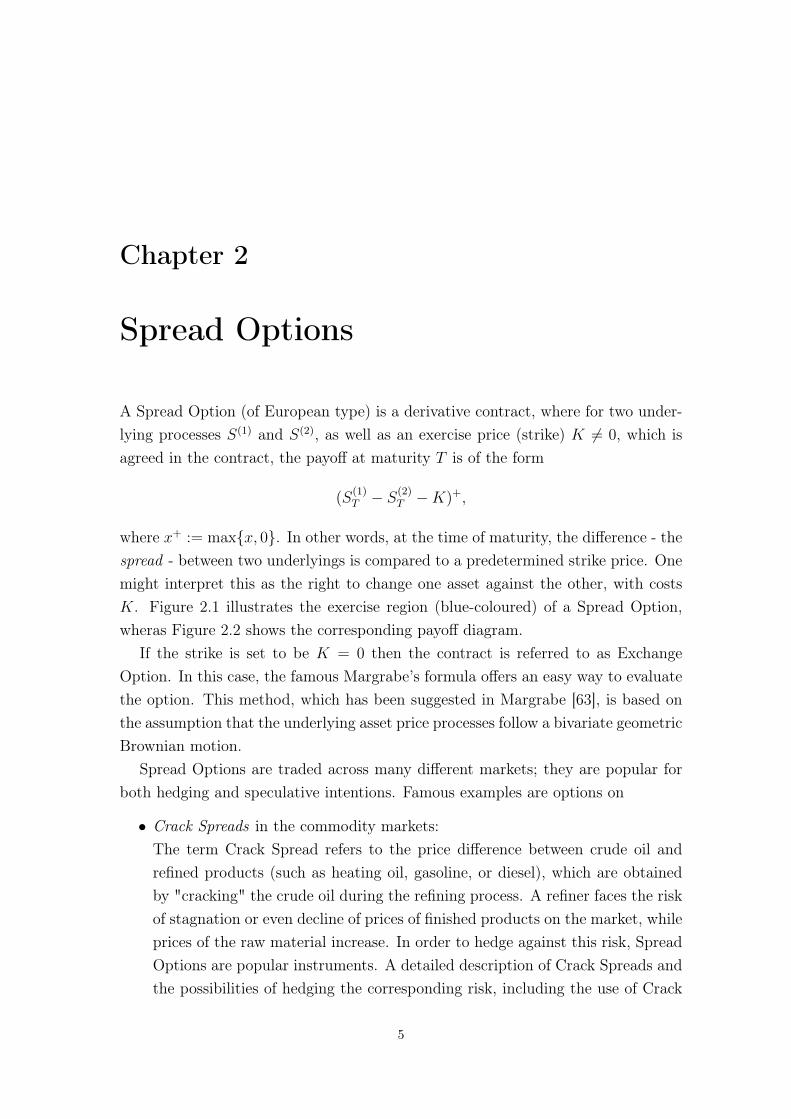
where x+ := maxx, 0. In other words, at the time of maturity, the difference - thespread - between two underlyings is compared to a predetermined strike price. Onemight interpret this as the right to change one asset against the other, with costsK. Figure 2.1 illustrates the exercise region (blue-coloured) of a Spread Option,wheras Figure 2.2 shows the corresponding payoff diagram.

If the strike is set to be K = 0 then the contract is referred to as ExchangeOption. In this case, the famous Margrabe’s formula offers an easy way to evaluatethe option. This method, which has been suggested in Margrabe [63], is based onthe assumption that the underlying asset price processes follow a bivariate geometricBrownian motion.

Spread Options are traded across many different markets; they are popular forboth hedging and speculative intentions. Famous examples are options on

• Crack Spreads in the commodity markets:The term Crack Spread refers to the price difference between crude oil andrefined products (such as heating oil, gasoline, or diesel), which are obtainedby "cracking" the crude oil during the refining process. A refiner faces the riskof stagnation or even decline of prices of finished products on the market, whileprices of the raw material increase. In order to hedge against this risk, SpreadOptions are popular instruments. A detailed description of Crack Spreads andthe possibilities of hedging the corresponding risk, including the use of Crack

5

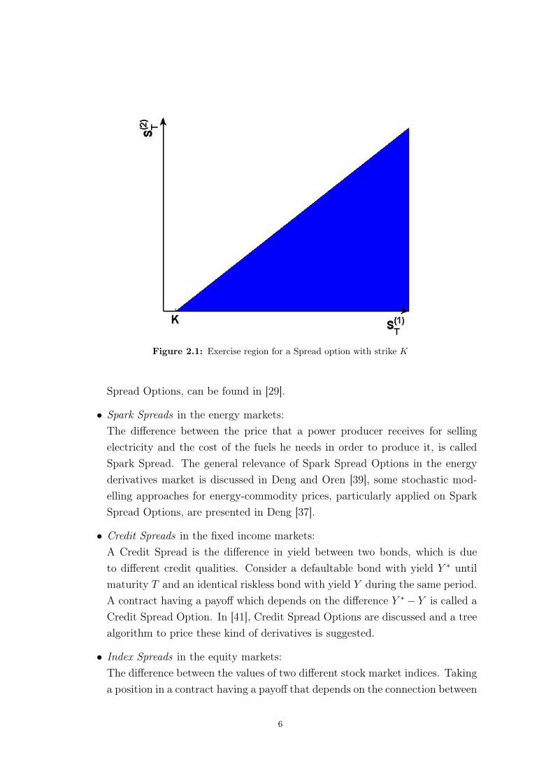
Figure 2.1: Exercise region for a Spread option with strike K

Spread Options, can be found in [29].

• Spark Spreads in the energy markets:The difference between the price that a power producer receives for sellingelectricity and the cost of the fuels he needs in order to produce it, is calledSpark Spread. The general relevance of Spark Spread Options in the energyderivatives market is discussed in Deng and Oren [39], some stochastic mod-elling approaches for energy-commodity prices, particularly applied on SparkSpread Options, are presented in Deng [37].

• Credit Spreads in the fixed income markets:A Credit Spread is the difference in yield between two bonds, which is dueto different credit qualities. Consider a defaultable bond with yield Y ∗ untilmaturity T and an identical riskless bond with yield Y during the same period.A contract having a payoff which depends on the difference Y ∗ − Y is called aCredit Spread Option. In [41], Credit Spread Options are discussed and a treealgorithm to price these kind of derivatives is suggested.

• Index Spreads in the equity markets:The difference between the values of two different stock market indices. Takinga position in a contract having a payoff that depends on the connection between

6

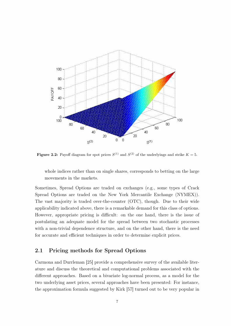
Figure 2.2: Payoff diagram for spot prices S(1) and S(2) of the underlyings and strike K = 5.

whole indices rather than on single shares, corresponds to betting on the largemovements in the markets.

Sometimes, Spread Options are traded on exchanges (e.g., some types of CrackSpread Options are traded on the New York Mercantile Exchange (NYMEX)).The vast majority is traded over-the-counter (OTC), though. Due to their wideapplicability indicated above, there is a remarkable demand for this class of options.However, appropriate pricing is difficult: on the one hand, there is the issue ofpostulating an adequate model for the spread between two stochastic processeswith a non-trivial dependence structure, and on the other hand, there is the needfor accurate and efficient techniques in order to determine explicit prices.

2.1 Pricing methods for Spread Options

Carmona and Durrleman [25] provide a comprehensive survey of the available liter-ature and discuss the theoretical and computational problems associated with thedifferent approaches. Based on a bivariate log-normal process, as a model for thetwo underlying asset prices, several approaches have been presented: For instance,the approximation formula suggested by Kirk [57] turned out to be very popular in

7

practice. A further analytic approximation formula is due to Carmona and Durrle-man [26]; they derive a family of lower as well as an upper price bound, which canyield a very tight interval. Venkatramanan and Alexander [85] suggest a methodwhere they obtain the price of a Spread Option as the sum of the prices of twocompound options, one of which is to exchange vanilla Call Options on the twounderlying assets and the other one is to exchange the corresponding Put Options.Other methods are, e.g., due to Pearson [69], Deng et al. [38], Borovka et al. [21],or Bjerksund and Stensland [19].

The available literature on Spread Option valuation for general models, i.e., with-out the assumption of a bivariate log-normal process, is rather sparse. The ansatzproposed by Dempster and Hong [36] was the first efficient method applicable tonon-Gaussian models. They extended the Fast Fourier transform technique of Carrand Madan [27] (see sect. 2.1.2) to a multi-factor setting, providing applicabilityfor instance to many models of the affine jump-diffusion type. Analogously to theidea of integrating by Riemann sums, they calculate the Spread Option price byforming tight upper and lower bounds for the integral over a non-polygonal region(the exercise region in logarithmic variables is non-linear).

Hurd and Zhou [51] have proposed a more elegant method as an extension of thelogic of Carr and Madan [27]: the core of their procedure is the representation theyderive of the Fourier transform of the Spread Option payoff function in terms of thecomplex Gamma function.

Most recently, Caldana and Fusai [24] have generalized the work of Bjerksundand Stensland [19] by deriving a lower bound approximation for the Spread Optionprice, which can be applied for any model, where the joint characteristic functionof the log-returns of the two underlying assets is available in closed form. Basically,the idea of this approach is the following: Define the event

A :=

ω :S

(1)T(

S(2)T

)α > ek

E[(S

(2)T

)α] ,

and consider the lower bound of the Spread Option payoff(S

(1)T − S

(2)T −K

)+

≥(S

(1)T − S

(2)T −K

)1A.

Extending the work of Bjerksund and Stensland [19], who worked in the bivari-ate GBM setting, Caldana and Fusai [24] suggest how to approximate the exactSpread Option price by Ck,α

K (0) := e−rTE[(S(1)T −S

(2)T −K)1A] (for a suitable choice

8

of the parameters k and α) for any stock price model, where the joint character-istic function of (logS

(1)T , logS

(2)T ) is available in closed form. In particular, they

give a representation of the approximate Spread Option price Ck,αK (0) in terms of

a Fourier inversion formula. Their bound has turned out to be very accurate andeasily computable. The authors argue that their method improves upon the one dueto Hurd and Zhou [51] on some points: First, unlike the Hurd and Zhou method,which is not applicable to Exchange Options (i.e., in the case K = 0), their pro-cedure also copes with this case. Second, Hurd and Zhou’s technique requires theassumption that the characteristic function of the log-asset price process Xt factor-izes as E[eiuXT |X0] = eiuX0E[eiu(XT−X0)]. This assumption rules out mean-revertingasset models, while there is no issue for Caldana and Fusai’s method regarding suchmodels. Third, Caldana and Fusai’s technique involves only a univariate Fourierinversion, rather than a bivariate one, as is the case for Hurd and Zhou’s approach.This improves the computational speed considerably, considering a single contract.

However, the advantages provided by the Caldana and Fusai method are notreally relevant for our purposes: The asset models considered in this thesis are notof mean-reverting nature (only the volatility processes are, but this is not an issue).Moreover, we want to study "real" Spread Options rather than Exchange Options.The improvement in terms of the computational speed may be true for a singlecontract; however, as is also admitted by the authors, considering the valuation ofmany contracts, Hurd and Zhou’s method will still be superior. They implement aninterpolation procedure, where the valuation of every further contract only requiresvery little time, while the computational cost for Caldana and Fusai’s lower boundincreases linearly in the number of evaluated contracts. Furthermore, even if it hasturned out to be very accurate for a number of asset models, Caldana and Fusai stillpropose a procedure to determine price bounds, while Hurd and Zhou aim for theexact price. For these reasons, we are going to follow the technique suggested byHurd and Zhou [51]. Now we want to explain this method in detail and previouslyalso give a general introduction to transform-based option pricing.

2.1.1 Fourier transform methods for option pricing

Let St = S0eXt be the price process of a risky asset. The arbitrage-free pricing

paradigm based on the Fundamental Theorem of Asset Pricing means that theprice at time zero of a claim with terminal payoff f(ST ) is the discounted expectedvalue of this payoff, where the expectation is taken with respect to an equivalent

9

martingale measure, i.e.,

V0 = e−rTEQT [f(ST )] = e−rT∫ ∞−∞

f(x)ρT (x)dx,

where ρT denotes the density of the log-returns under the risk-neutral pricing mea-sure QT . However, in many models, this density ρT is not available; the probabilitydensity of a Lévy processes, for example, is typically not known in closed form. Onthe other hand, the characteristic function of the process is in most cases availablein terms of elementary functions. Therefore, one wants to work with representa-tions, where the distribution of the log-returns appears in terms of its characteristicfunction. The concrete idea is the following: If the payoff f(ST ) can be representedas an integral of the form

∫g(z)(ST )zdz, and the moment generating function1 ΦXT

of the log-returns is available in closed form, then we can write

V0 = e−rT∫g(z)EQT [(ST )z]dz

= e−rT∫g(z)EQT [ezXT ](S0)zdz

= e−rT∫g(z)ΦXT (z)(S0)zdz.

Hence, the price can be determined by a one-dimensional (numerical) integration.The desired representation of the payoff can, e.g., be obtained by using the Fouriertransform.

The d-dimensional Fourier transform of a function f is, for v ∈ Rd, defined by

Ff(x)(v) =

∫ ∞−∞· · ·∫ ∞−∞

eiv>xf(x) dx1 · · · dxd.

The function f can be "recovered" by the corresponding Fourier inversion, which isgiven by

f(x) =1

(2π)d

∫ ∞−∞· · ·∫ ∞−∞

e−ix>v Ff(x)(v) dv1 · · · dvd.

2.1.2 Using the Fast Fourier transform for option pricing: The methodof Carr and Madan

In order to explain the idea, we first consider a Call Option on the underlying assetprice St, with maturity T and strike K. Let k := logK, sT := logST , and denote

1We use the moment generating function here for ease of notation; due to the relationship Φ(z) = φ(−iz) to thecharacteristic function, the same lines can of course analogously be written in terms of φ.

10

the risk-neutral density of the log-asset price by qT . The following strategy is alongthe lines of Carr and Madan [27]:

The value of the Call Option at time zero is given by

CT (k) = e−rT∫ ∞−∞

(ex − ek)+qT (x)dx = e−rT∫ ∞k

(ex − ek)qT (x)dx.

However, the Call price as a function in k is not (square-)integrable, since

limk→−∞

CT (k) = limk→−∞

e−rT∫ ∞k

(ex − ek)qT (x)dx

= e−rT∫ ∞−∞

exqT (x)dx

= EQT [e−rTST ]

= S0.

L1-integrability of a function is however a sufficient condition for its Fourier trans-form to exist. The idea in order to avoid this problem is to modify the Call-pricingfunction in terms of choosing some α > 0 and working with the "damped" function

cT (k) := eαkCT (k)

instead. If we now consider the Fourier transform of cT (k), which can be written as

ψT (v) =

∫ ∞−∞

eivkcT (k)dk

=

∫ ∞−∞

eivkeαk(e−rT

∫ ∞k

(ex − ek)qT (x)dx

)dk

=

∫ ∞−∞

e−rT qT (x)

∫ x

−∞(ex+αk − e(1+α)k)eivkdk dx

=

∫ ∞−∞

e−rT qT (x)

(e(α+1+iv)x

α + iv− e(α+1+iv)x

α + 1 + iv

)dx

=e−rT

(α + iv)(α + 1 + iv)

∫ ∞−∞

qT (x)e(α+1+iv)xdx

=e−rT

α2 + α− v2 + iv(2α + 1)

∫ ∞−∞

ei(−i(α+1)+v)xqT (x)dx

=e−rTφT (v − i(α + 1))

α2 + α− v2 + iv(2α + 1), (2.1)

then we can represent the option price by Fourier inversion of ψT (v) (and undamp-

11

ing) as

CT (k) = e−αkcT (k) = e−αk1

2π

∫ ∞−∞

e−ivkψT (v)dv

=exp(−αk)

π

∫ ∞0

e−ivkψT (v)dv, (2.2)

where we have a closed-form expression of ψT (v) at hand by (2.1). The last equalityholds due to the fact that option prices are real, which means that the imaginarypart must vanish, which in turn is the case if the integrand is odd in its imaginarypart (for any integration limits symmetrical to the origin). On the other hand, itsreal part is even, which implies that the integrals over the two half-axes coincide.

In order to obtain an explicit price for the Call Option, we are only left withthe evaluation of the integral in (2.2). An easy way for approximating this integralis to apply the rectangle rule: Fix N , choose a step size η, set vj = η(j − 1) forj = 1, . . . , N , and use the approximation

CT (k) ≈ exp(−αk)

π

N∑j=1

e−ivjkψT (vj)η. (2.3)

The Fast Fourier transform (FFT) is an efficient algorithm for computing a discreteFourier transform (DFT), i.e., a sum of the form

X(k) =N∑j=1

e−i 2πN

(j−1)(k−1)x(j) for k = 1, . . . , N, (2.4)

for an input vector x = (x1, . . . , xN), and where N is (typically) a power of 2.The FFT algorithm reduces the number of operations necessary to compute (2.4)from O(N2) (corresponding to computing all the sums directly) to O(N logN).Particularly due to the fact that, with respect to (2.3), this would correspond toobtaining prices for a whole range of N different strike values in a very fast way(i.e., with just one evaluation of the very efficient FFT), it is appealing to use theFast Fourier transform.

The possibility of evaluating discrete Fourier transforms in an efficient way hasbeen crucial for many applications; FFT algorithms are among the most importantalgorithms in various applied fields. There are many different versions of FFTalgorithms available, however, the original2 formulation due to Cooley and Tukey

2In fact, it has been discovered that a similar idea had already been used by Gauss at the beginning of thenineteenth century, but was not really noticed for a long time (cf. Heidemann et al. [44]).

12

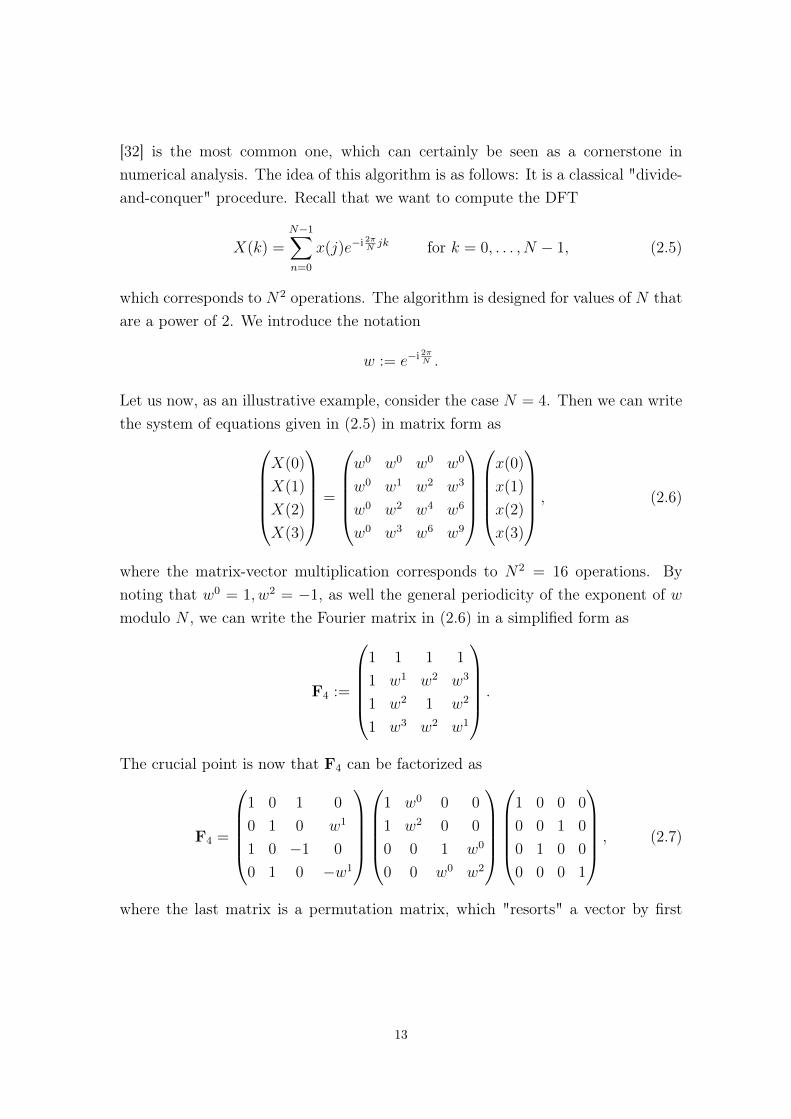
[32] is the most common one, which can certainly be seen as a cornerstone innumerical analysis. The idea of this algorithm is as follows: It is a classical "divide-and-conquer" procedure. Recall that we want to compute the DFT

X(k) =N−1∑n=0

x(j)e−i 2πNjk for k = 0, . . . , N − 1, (2.5)

which corresponds to N2 operations. The algorithm is designed for values of N thatare a power of 2. We introduce the notation

w := e−i 2πN .

Let us now, as an illustrative example, consider the case N = 4. Then we can writethe system of equations given in (2.5) in matrix form as

X(0)

X(1)

X(2)

X(3)

=

w0 w0 w0 w0

w0 w1 w2 w3

w0 w2 w4 w6

w0 w3 w6 w9

x(0)

x(1)

x(2)

x(3)

, (2.6)

where the matrix-vector multiplication corresponds to N2 = 16 operations. Bynoting that w0 = 1, w2 = −1, as well the general periodicity of the exponent of wmodulo N , we can write the Fourier matrix in (2.6) in a simplified form as

F4 :=

1 1 1 1

1 w1 w2 w3

1 w2 1 w2

1 w3 w2 w1

.

The crucial point is now that F4 can be factorized as

F4 =

1 0 1 0

0 1 0 w1

1 0 −1 0

0 1 0 −w1

1 w0 0 0

1 w2 0 0

0 0 1 w0

0 0 w0 w2

1 0 0 0

0 0 1 0

0 1 0 0

0 0 0 1

, (2.7)

where the last matrix is a permutation matrix, which "resorts" a vector by first

13

listing all even components, then followed by all the odd ones, i.e.,1 0 0 0

0 0 1 0

0 1 0 0

0 0 0 1

x(0)

x(1)

x(2)

x(3)

=

x(0)

x(2)

x(1)

x(3)

.

We notice from equation (2.7) that F4 is of the form

F4 =

(I2 W2

I2 −W2

)(F2 0

0 F2

)(permutation

matrix

),

where I2 is the (2-dim.) identity matrix, W2 =

(1 0

0 w1

), and F2 =

(1 w0

w0 w2

).

Therefore, we have reduced the number of operations from N2 = 16 to 2(N2

)2=

N2

2= 8.The factorization we just performed on F4, where we split the problem into two

smaller problems of half size, resulting in a reduction of the number of computationaloperations, is generally applicable; it yields the recursion

Fn =

(In/2 Wn/2

In/2 −Wn/2

)(Fn/2 0

0 Fn/2

)(permutation

matrix

),

whereWn/2 = diag(w0, w1, . . . , wn/2−1). Hence, the problem of a DFT of size N canbe fully reduced to two DFT’s, each of size N/2. Since we assumed that N = 2m,after m = log2N steps, a DFT of size N can be reduced to N Fourier transforms,each of size 1. Due to the fact that the Fourier transform of a single number is thenumber itself (see equation (2.5) for N = 1), the algorithm terminates trivially. Thismeans that there is a total of log2N "stages" of computation. Each of them requiresO(N) complex operations. Therefore, the FFT algorithm reduces the number ofoperations required to evaluate a DFT from O(N2) to O(N logN).

Let us now get back to the aim of evaluating the option by applying the FFT inorder to compute (2.2): We choose a step size λ in the "strike-world" and considerthe values ku for k along a regularly-spaced grid, which are given by

ku = −b+ λ(u− 1), for u = 1, . . . , N,

14

where b = Nλ2. Consequently, for u = 1, . . . , N , we get

CT (ku) ≈exp(−αku)

π

N∑j=1

e−ivj(−b+λ(u−1))ψT (vj)η,

=exp(−αku)

π

N∑j=1

e−iλη(j−1)(u−1)eibvjψT (vj)η.

(2.8)

Thus, if we choose the "Fourier grid" and the "strike grid" such that

λη =2π

N,

then we can apply the FFT (cf. (2.4)) on (2.8) and we obtain as a result all thevalues CT (ku), for u = 1, . . . , N .

An alternative approach regarding the integrability issue

The approach explained above makes use of a damping factor eαk and works withthe damped Call pricing function cT (k) = eαkCT (k), since the function CT (k) itselfis not in L1. Another way of circumventing the lacking integrability is to work withtime-values instead of damped option prices. This idea is also due to Carr andMadan [27]. They suggested it, since they noticed that for short maturities andstrike values far from the at-the-money level, the integrand in (2.2) becomes highlyoscillatory, and hence difficult to integrate numerically. We want to explain thistechnique here, since we will come back to this idea at a later stage. The particularstrategy is the following:

The time-value of an option is defined as the option price subtracted by theintrinsic value. It can be interpreted as the premium an investor pays over thecurrent exersice value of the option. Naturally, the time-value decays exponentiallyto zero when approaching maturity. Let now

zT (k) := e−rTEQT[(eXT − ek

)+]−(1− ek

)+

be the time-value of a Call Option as a function in the log-strike k, and denote itsFourier transform by

ζT (v) := FzT (k)(v) =

∫ ∞−∞

eivkzT (k)dk. (2.9)

15

Exploiting the fact that the discounted price process is a QT -martingale, we get

zT (k) = e−rT∫ ∞−∞

ρT (x)(ex − ek)1k≤x dx− (1− ek)1k≤0

= e−rT∫ ∞−∞

ρT (x)(ex − ek)(1k≤x − 1k≤0) dx.

If we plug this representation of zT (k) into (2.9) then we can write3

ζT (v) = e−rT∫ ∞−∞

ρT (x)

(∫ x

0

eivk(ex − ek)dk)dx

= e−rT∫ ∞−∞

ρT (x)

((1− ex)1 + iv

+iex

(1 + iv)v− iex+ivx

(1 + iv)v

)dx

= e−rT(

1− EQT [ST ]

1 + iv+

i

(1 + iv)v

(EQT [ST ])−

∫ ∞−∞

ρT (x)ei(v−i)xdx

))=

e−rT

1 + iv− 1

1 + iv+

i

(1 + iv)v− ie−rTφT (v − i)

(1 + iv)v

=e−rT

1 + iv+

−v + i

(i− v)(−iv)− e−rTφT (v − i)

v(v − i)

= e−rT(

1

1 + iv− erT

iv− φT (v − i)

v(v − i)

).

With this closed-form expression of the Fourier transform at hand, we can againproceed as before; we obtain option prices by numerically inverting the Fouriertransform (with possible use of the FFT analogously to above).

2.1.3 The method of Hurd and Zhou for Spread Option pricing

Hurd and Zhou [51] have extended the idea of Carr and Madan, i.e, the application ofthe FFT for option-pricing, to two dimensions: they propose an efficient strategy forthe pricing of Spread Options. The core of their work is the following theorem, whichgives a representation of the Fourier transform of the payoff of a Spread Option interms of the complex Gamma function. Since we will follow their strategy for ournumerical studies in chapter 5, we also want to explain the proof of this centralresult in detail.

Theorem 2.1: Let P (x1, x2) = (ex1 − ex2 − 1)+ be the payoff function of a SpreadOption with strike 1. Then, for any vector of real numbers ε = (ε1, ε2) with ε2 > 0

3In order to ensure the feasibility of all the rearrangements, particularly, of the interchanging of the integrationorder, the following technical condition must be assumed: ∃ α > 0 :

∫∞−∞ ρT (x)e(1+α)xdx < ∞. However, as

contrary to the strategy with the damping factor, we do not need to choose a specific value of α in order to obtainthe option price.

16

and ε1 + ε2 < −1 and x = (x1, x2), the payoff function has the representation

P (x) =1

(2π)2

∫ ∫R2+iε

eiuxtP (u)d2u, (2.10)

where

P (u) =Γ(i(u1 + u2)− 1)Γ(−iu2)

Γ(iu1 + 1).

Here, Γ(z) denotes the complex Gamma function defined for Re(z) > 0 by theintegral Γ(z) =

∫∞0e−ttz−1dt.

Proof. Let ε2 > 0 and ε1 + ε2 < −1. Application of the Fourier inversion theoremon eεxP (x) (the factor eεx ensures that this is in L2(R2)) yields

eεxP (x) = F−1FeεxP (x)(u)(x)

=1

2π

∫R

∫Reiux

∫R

∫Re−iuxeεxP (x)du1du2dx1dx2

=1

2π

∫R2

eεxei(u+iε)x

∫R2

e−i(u+iε)xP (x)d2xd2u

=1

2πeεx∫R2+iε

eiux

∫R2

e−iuxP (x)d2xd2u

= eεx(

1

2π

∫R2+iε

eiuxg(u)d2u

).

Therefore,

P (x) =1

2π

∫R2+iε

eiuxg(u)d2u,

where

g(u) =

∫R2

e−iuxP (x)d2x.

The payoff function P (x) = (ex1 − ex2 − 1)+ means that the domain of the integralcan be restricted to x = (x1, x2) : x1 > 0, ex2 < ex1 − 1, and the function g canbe hence be written as

g(u) =

∫ ∞0

e−iu1x1

(∫ log(ex1−1)

−∞e−iu2x2(ex1 − ex2 − 1)dx2

)dx1

=

∫ ∞0

e−iu1x1(ex1 − 1)1−iu2

(1

−iu2

− 1

1− iu2

)dx1.

17

Substituting e−x1 by z leads to

g(u) =1

(1− iu2)(−iu2)

∫ 1

0

ziu1

(1− zz

)1−iu2 dz

z.

Using the Beta function

B(a, b) =Γ(a)Γ(b)

Γ(a+ b),

which is defined on a, b ∈ C : Re(a),Re(b) > 0 as

B(a, b) =

∫ 1

0

za−1(1− z)b−1dz,

and the property Γ(z) = (z−1)Γ(z−1) of the Gamma function, the function g canfurther be written as

g(u) =Γ(i(u1 + u2)− 1)Γ(−iu2 + 2)

(1− iu2)(−iu2)Γ(iu1 + 1)

=Γ(i(u1 + u2)− 1)(−iu2 + 1)(−iu2)Γ(−iu2)

(1− iu2)(−iu2)Γ(iu1 + 1)

=Γ(i(u1 + u2)− 1)Γ(−iu2)

Γ(iu1 + 1).

If we assume that the process X has independent and stationary increments (thisasssumption will hold true for all models studied in chapter 4), we can use (2.10)to obtain the following representation of the price of a Spread Option:

Spr(X0;T ) = E[e−rTP (XT )|F0]

= e−rTE[

(2π)−2

∫ ∫R2+iε

eiuXtT P (u)d2u

∣∣∣∣F0

]= (2π)−2e−rT

∫ ∫R2+iε

eiuXt0E[eiu(XT−X0)t

∣∣∣F0

]P (u)d2u

= (2π)−2e−rT∫ ∫

R2+iε

eiuXt0E[eiuXt

T

]P (u)d2u

=1

(2π)2e−rT

∫ ∫R2+iε

eiuXt0φXT (u)P (u)d2u. (2.11)

For a numerical evaluation of the double integral in 2.11, the authors of [51] suggestto follow the logic of Carr and Madan (see section 2.1.2) in the following way: In

18

the two-dimensional setting it means an approximation of the double integral bychoosing a truncation interval [−u, u], as well as a number of steps N (we will alwaysuse powers of 2, which is a convenient choice and ensures that N is even, what willbe assumed implicitly for some rearrangements in the sequel) within this interval,and evaluating the double sum over the corresponding lattice

Γ = u(k) = (u1(k1), u2(k2)) | k = (k1, k2) ∈ 0, . . . , N − 1 × 0, . . . , N − 1,

with ui(ki) = −u+ kiη, and where η is the step size, resulting from the choice of uand N , by η = 2u/N . The reciprocal lattice is given by

Γ∗ = x(l) = (x1(l1), x2(l2)) | l = (l1, l2) ∈ 0, . . . , N − 1 × 0, . . . , N − 1,

with xi(ki) = −x+ liη∗, and where η∗ = 2π/(Nη) = π/u and x = Nη∗/2.

In particular, under the assumption that the vector of the logarithmic initial valuesof the underlying asset is lying on the lattice Γ∗, i.e., that there exists a vectorl∗ = (l∗1, l

∗2) ∈ 0, . . . , N − 12 such that X0 = x(l∗) ∈ Γ∗, for S0 = eX0 , a simple

application of the rectangle method on the double integral in (2.11) yields

Spr(X0;T ) ≈ η2e−rT

(2π)2

N−1∑k1=0

N−1∑k2=0

ei(u(k)+iε)x(l∗)tφXT (u(k) + iε)P (u(k) + iε). (2.12)

The exponential function in (2.12) can be written as

ei(u(k)+iε)x(l∗)t = e−εx(l∗)tei(u1(k1)x1(l∗1)+u2(k2)x2(l∗2))

= e−εx(l∗)t · exp (i ((−u+ k1η)(−x+ l∗1η∗) + (−u+ k2η)(−x+ l∗2η

∗)))

= e−εx(l∗)t · exp(i((−Nη2

+ k1η)(−πη

+ l∗1η∗) + (−Nη

2+ k2η)(−π

η+ l∗2η

∗)))

= e−εx(l∗)t · eiπN · e−iπ(k1+k2+l∗1+l∗2) · e2πiN

(k1l∗1+k2l∗2)

= e−εx(l∗)t · (−1)iπ(k1+k2+l∗1+l∗2) · e2πikl∗t/N ,

which leads to the representation

Spr(X0;T ) ≈ (−1)l∗1+l∗2e−rT

(ηN

2π

)2

e−εx(l∗)t

[1

N2

N−1∑k1,k2=0

e2πikl∗tN h(k)

], (2.13)

where

h(k) = (−1)k1+k2φXT (u(k) + iε)P (u(k) + iε).

19

The term in square brackets on the right hand side of equation (2.13) is now ofa form such that it corresponds exactly to that value of a double inverse discreteFourier transform of the function h, which corresponds to l∗. The double inversediscrete Fourier transform can be efficiently computed by using the FFT algorithm,and is a standard-routine in all well-known software packages. In MATLAB, forinstance, the function4 ifft2() applied on the N ×N -dimensional input array H,where H[k1, k2] := h(k) for k = (k1, k2) ∈ 0, . . . , N − 12, yields the output arrayY , where, for l = (l1, l2) ∈ 0, . . . , N − 12,

Y [l] =1

N2

N−1∑k1,k2=0

e2πiklt

N H[k].

In this way, one gets prices for Spread Options with strike 1 and log-initial val-ues X(1)

0 , X(2)0 lying on Γ∗. The assumption regarding the strike is, in fact, not a

curtailment of generality: For a general strike K ∈ R, we can write

Spr(X0;T ) = E[e−rT (S(1)T − S

(2)T −K)+]

= K · e−rTE[(S(1)T /K − S(2)

T /K − 1)+]

= K · e−rTE[(eX(1)T − eX

(2)T − 1)+],

which means that by setting X(1) := log(S(1)/K) and X(2) := log(S(2)/K) insteadof log(S(1)) resp. log(S(2)), i.e., by using "moneyness" instead of the absolute valuesof the underlying assets, we can use the pricing procedure for a Spread Option withstrike 1 as described above and simply have to multiply the resulting option priceby K.

The assumption that both of the log-initial values X(1)0 and X(2)

0 exactly lie onthe lattice in the Fourier-space, is of theoretical nature, though. In practice, ifone wants to use this method for the pricing of arbitrary Spread Option contracts(as we will do in chapter 5), one has to think about how to deal with any givenset S(1)

0 , S(2)0 , K. We want to use two different approaches: The first one is to

choose the lattice Γ, i.e., the lattice in the Fourier-space, not just by specifyingany truncation interval and the number of steps, but rather exactly in such a waythat the log-initial values fall on grid points of Γ(∗). In particular, we do this inthe following way: We first fix the number of steps N and the truncation-interval"roughly" as [−u0, u0]. Then, for each of the two assets, we keep stretching the

4One needs to be careful when using these built-in functions: in different software packages, Fouriertransforms are implemented with different parameters. In MATHEMATICA, for example, the functionInverseFourier corresponds to MATLAB’s ifft; however, exact correspondence is only given if one uses theoption InverseFourier[...,FourierParameters->1,-1].

20

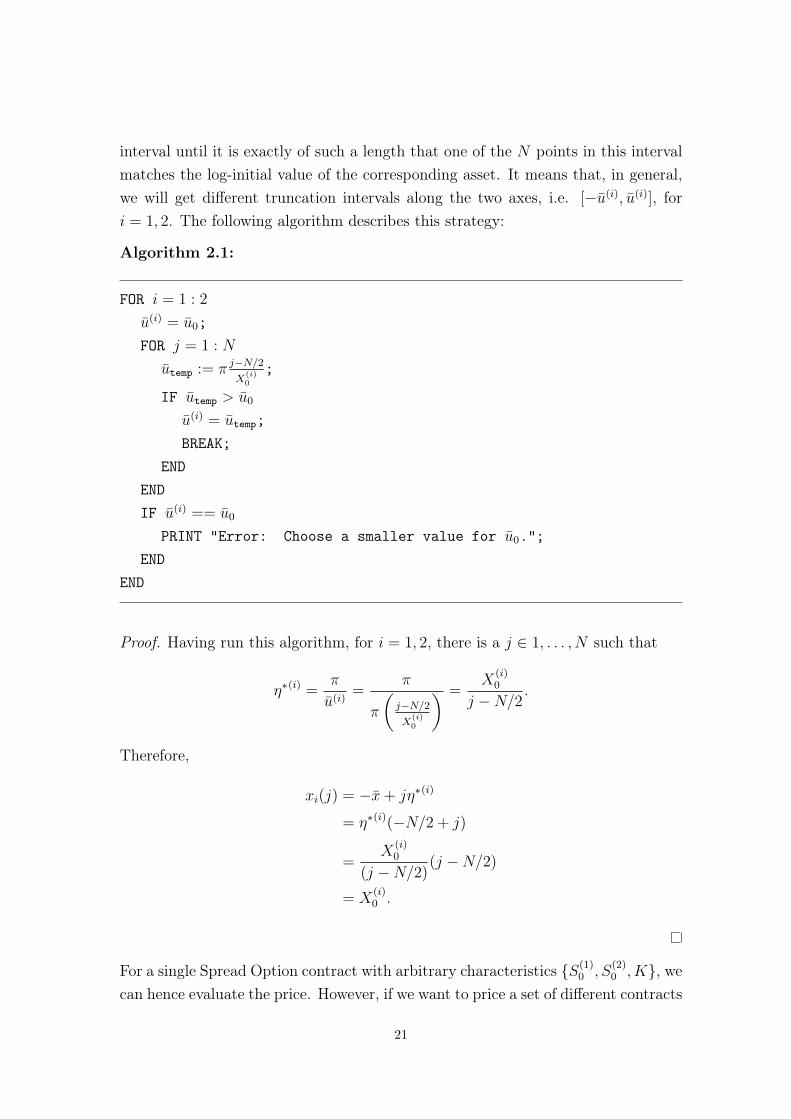
interval until it is exactly of such a length that one of the N points in this intervalmatches the log-initial value of the corresponding asset. It means that, in general,we will get different truncation intervals along the two axes, i.e. [−u(i), u(i)], fori = 1, 2. The following algorithm describes this strategy:

Algorithm 2.1:

FOR i = 1 : 2

u(i) = u0;FOR j = 1 : N

utemp := π j−N/2X

(i)0

;

IF utemp > u0

u(i) = utemp;BREAK;

ENDENDIF u(i) == u0

PRINT "Error: Choose a smaller value for u0.";END

END

Proof. Having run this algorithm, for i = 1, 2, there is a j ∈ 1, . . . , N such that

η∗(i) =π

u(i)=

π

π

(j−N/2X

(i)0

) =X

(i)0

j −N/2.

Therefore,

xi(j) = −x+ jη∗(i)

= η∗(i)(−N/2 + j)

=X

(i)0

(j −N/2)(j −N/2)

= X(i)0 .

For a single Spread Option contract with arbitrary characteristics S(1)0 , S

(2)0 , K, we

can hence evaluate the price. However, if we want to price a set of different contracts

21

(think of a calibration of model parameters, for instance, where one usually needsto calculate prices for a lot of different options at the same time), we will need torun the whole selection procedure of the lattice as well as the Fourier inversion forevery single contract. This coincides with an increase in computation time.Therefore, as an alternative approach, we want to exploit that, in fact, with everyFourier inversion we get a whole N×N matrix of prices, corresponding to contractswith characteristics ex1(l1), ex2(l2), K, for l = (l1, l2) ∈ 0, . . . , N − 12. Givenall those prices, we can approximate any contract with S

(i)0 ∈ [minexi(li) : li ∈

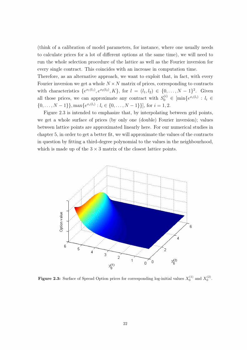
0, . . . , N − 1,maxexi(li) : li ∈ 0, . . . , N − 1], for i = 1, 2.Figure 2.3 is intended to emphasize that, by interpolating between grid points,

we get a whole surface of prices (by only one (double) Fourier inversion); valuesbetween lattice points are approximated linearly here. For our numerical studies inchapter 5, in order to get a better fit, we will approximate the values of the contractsin question by fitting a third-degree polynomial to the values in the neighbourhood,which is made up of the 3× 3 matrix of the closest lattice points.

Figure 2.3: Surface of Spread Option prices for corresponding log-initial values X(1)0 and X(2)

0 .

22

Chapter 3

Theory of Lévy Processes andMarket Modelling

3.1 Lévy Processes

3.1.1 A review of general theory

Definition 3.1 (Lévy Process): A stochastic process X = (Xt)t≥0 on a probabilityspace (Ω,F ,P) is called a Lévy process, if it satisfies the following conditions:

1. X0 = 0, P-a.s.

2. The increments are independent:For any increasing series of times t0, t1, . . . , tn, the random variables Xt0 , Xt1−Xt0 , . . . , Xtn −Xtn−1 are independent.

3. The increments are stationary:For any t1, t2, h ≥ 0, it holds that Xt1+h − Xt1

d= Xt2+h − Xt2. In particular,

the distribution of the increment Xt+h −Xt does not depend on t.

4. X is stochastically continuous:∀ε > 0 : lim

h→0P [|Xt+h −Xt| ≥ ε] = 0.

The requirement of stochastic continuity means that the probability of a discon-tinuity in the trajectory, at a given concrete time t, equals zero, i.e., jumps onlyoccur randomly. Brownian motion is the only Lévy process having indeed continu-ous sample paths.

The distribution of the increments of a Lévy process cannot be chosen arbitrarily;there are constraints on feasible choices, in particular, the distribution of Xt has tobe infinitely divisible. The formal statement is given below in Proposition 3.1.

23

Definition 3.2 (Infinite divisibility): A probability distribution µ is called infinitelydivisible if for any n ∈ N, n ≥ 2, there exist independent and identically distributedrandom variables Y1, . . . , Yn such that the distribution of the sum Y1 + . . . + Yn isgiven by µ.

Proposition 3.1 (Infinite divisibility and Lévy processes (cf. [31], Prop. 3.1)): LetX = (Xt)t≥0 be a Lévy process. Then for any given time t, the distribution of Xt isinfinitely divisible. Conversely, for any given infinitely divisible distribution µ thereexists a Lévy process X such that the distribution of X1 is given by µ.

Two cornerstones of the theory of Lévy processes are the so-called Lévy-Khintchineformula (see Theorem 3.2), which describes the distributional properties of a Lévyprocess by giving a representation of its characteristic function, and the Lévy-Itodecomposition (see Theorem 3.1), which gives indication of the structure of thetrajectories of the process.

Definition 3.3 (Lévy measure): For a Lévy process X = (Xt)t≥0 with jumps ∆Xt =

Xt −Xt−, its Lévy measure ν is defined as

ν(A) := E[#t ∈ (0, 1] : 0 6= ∆Xt ∈ A], ∀A ∈ B(R).

Definition 3.4 (Poisson random measure): Let (Ω,F ,P) be a propability space anddefine MN(R× [0,∞)) := µ : µ is a measure on R× [0,∞); µ(A× I) ∈ N, ∀A ∈B(R), ∀I ∈ B([0,∞)). A mapping N : Ω → MN(R × [0,∞)) is called a Poissonrandom measure if

1. ∀A ∈ B(R), ∀I ∈ B([0,∞)):N(A× I) is a Poisson random variable with parameter ν(A) · λ(I)

(λ denoting the Lebesgue measure, ν(A) <∞).

2. ∀A1 × I1, A2 × I2 ∈ B(R)× B([0,∞)) with A1 × I1 ∩ A2 × I2 = ∅:

• N(A1 × I1) and N(A2 × I2) are independent,

• N(A1 × I1 ∪ A2 × I2) = N(A1 × I1) +N(A2 × I2).

Definition 3.5 (Compensated Poisson random measure): Let N be a Poisson ran-dom measure. Then its compensated measure N is defined as

N(A× I) := N(A× I)− ν(A) · λ(I).

Theorem 3.1 (Lévy-Ito decomposition; cf. [3], Prop. 3.7): Let X = (Xt)t≥0 be aLévy process on Rd. Then there exists a vector γ ∈ Rd, a d-dimensional Brownian

24

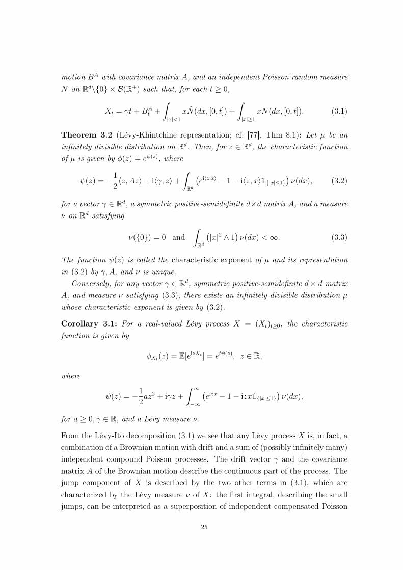
motion BA with covariance matrix A, and an independent Poisson random measureN on Rd\0 × B(R+) such that, for each t ≥ 0,

Xt = γt+BAt +

∫|x|<1

xN(dx, [0, t]) +

∫|x|≥1

xN(dx, [0, t]). (3.1)

Theorem 3.2 (Lévy-Khintchine representation; cf. [77], Thm 8.1): Let µ be aninfinitely divisible distribution on Rd. Then, for z ∈ Rd, the characteristic functionof µ is given by φ(z) = eψ(z), where

ψ(z) = −1

2〈z, Az〉+ i〈γ, z〉+

∫Rd

(ei〈z,x〉 − 1− i〈z, x〉1|x|≤1

)ν(dx), (3.2)

for a vector γ ∈ Rd, a symmetric positive-semidefinite d×d matrix A, and a measureν on Rd satisfying

ν(0) = 0 and∫Rd

(|x|2 ∧ 1

)ν(dx) <∞. (3.3)

The function ψ(z) is called the characteristic exponent of µ and its representationin (3.2) by γ,A, and ν is unique.

Conversely, for any vector γ ∈ Rd, symmetric positive-semidefinite d× d matrixA, and measure ν satisfying (3.3), there exists an infinitely divisible distribution µwhose characteristic exponent is given by (3.2).

Corollary 3.1: For a real-valued Lévy process X = (Xt)t≥0, the characteristicfunction is given by

φXt(z) = E[eizXt ] = etψ(z), z ∈ R,

where

ψ(z) = −1

2az2 + iγz +

∫ ∞−∞

(eizx − 1− izx1|x|≤1

)ν(dx),

for a ≥ 0, γ ∈ R, and a Lévy measure ν.

From the Lévy-Ito decomposition (3.1) we see that any Lévy process X is, in fact, acombination of a Brownian motion with drift and a sum of (possibly infinitely many)independent compound Poisson processes. The drift vector γ and the covariancematrix A of the Brownian motion describe the continuous part of the process. Thejump component of X is described by the two other terms in (3.1), which arecharacterized by the Lévy measure ν of X: the first integral, describing the smalljumps, can be interpreted as a superposition of independent compensated Poisson

25

processes, while the second integral, describing the large jumps of X, is a compoundPoisson process. The number of jumps with an absolute value greater than one isfinite, which we particularly know from (3.3). The triplet [γ,A, ν] consisting of thelinear drift, the Gaussian covariance matrix and the Lévy measure, respectively,which uniquely determines the distribution of a Lévy process, is called characteristictriplet or Lévy triplet of X. If the Brownian component is zero, we call X a Lévyjump process, if the drift term is zero as well, X is called a Lévy pure jump process.

In addition to infinite divisibility, another property classifying probability distribu-tions and, in further consequence, Lévy processes, is represented by the concept ofselfdecomposability. Selfdecomposable distributions will play a crucial role when weinvestigate OU type SV models, due to the fact that the class of selfdecomposabledistributions and the class of stationary distributions of OU processes (which aredriven by general Lévy processes) coincide. However, let us proceed step by step.

Definition 3.6 (Selfdecomposability): Let µ be a probability measure on R anddenote its characteristic function by φµ. Then µ is said to be selfdecomposable orto belong to Lévy’s class L, if for all t ∈ R and all c ∈ (0, 1) there exists a probabilitymeasure µc on R, with corresponding characteristic function φµc, such that

φµ(t) = φµ(ct)φµc(t). (3.4)

Remark: Selfdecomposability in terms of random variables means that given a ran-dom variable X, for any c ∈ (0, 1) there exists a random variable Xc, independentof X, such that

Xd= cX +Xc.

Remark: A Lévy process corresponding to a selfdecomposable distribution is calleda selfdecomposable process.

Selfdecomposability is a stronger concept than infinite divisibility. More specifically,one important relation can be formulated as follows:

Proposition 3.2 (cf. [77], Prop. 15.5): All probability measures µ ∈ L are infinitelydivisible, i.e., for any n ≥ 1 there exists a characteristic function φn such that

φ(t) = (φn(t))n ∀t ∈ R.

Furthermore, for any c ∈ (0, 1), µc in (3.4) is uniquely determined and infinitelydivisible.

26

The converse statement, that is a necessary and sufficient condition for a probabilitymeasure to be selfdecomposable, is given in the next proposition.

Proposition 3.3: A probability measure µ on R is selfdecomposable, if and only ifit is infinitely divisible with Lévy triplet [γ,A, ν], where γ ∈ R, A ≥ 0, and the Lévymeasure ν is of the form

ν(dx) =k(x)

|x|dx,

for a nonnegative function k(x), which is increasing on (−∞, 0) and decreasing on(0,∞).

For a proof of Proposition 3.2 and Proposition 3.3, and a comprehensive discussionof the concept of selfdecomposability of probability measures in general, see thebook of Sato [77]. Further interesting remarks on the class L and its relevance invarious contexts are explained by Jurek [53]. One critical characteristic of the classL is given in the subsequent theorem, which is due to Jurek and Vervaat [54]: therelation between selfdecomposability and Lévy processes.

Theorem 3.3: A random variable X has law in L if and only if X has a represen-tation of the form

X =

∫ ∞0

e−tdZt,

where Z = (Zt)t≥0 is a Lévy process.In this case, the resp. Lévy measures ν and ρ of X and Z1 are related by

ν(dx) =

∫ ∞0

ρ(etdx)dt.

We call Z the background driving Lévy process or, in short, the BDLP correspond-ing to X.

We now also formulate the above relation in terms of the corresponding Lévy den-sities (cf. [6]), since we will use it in this form at a later stage, that is in the contextof constructing Ornstein-Uhlenbeck processes.

Proposition 3.4: Suppose that the Lévy density f corresponding to ν is differen-tiable. Then the Lévy measure ρ has a density g, and f and g are related by

g(x) = −f(x)− xf ′(x). (3.5)

27

Using the notation

ν+(x) := ν([x,∞)) =

∫ ∞x

f(y)dy (3.6)

for the upper tail integral of the Lévy density, in Barndorff-Nielsen [5] it is derivedfrom the above formulae that

ν+(x) = xg(x).

The inverse function of ν+, denoted by ν−1, is given by

ν−1(x) = infy > 0 : ν+(y) ≤ x. (3.7)

3.1.2 Increasing Lévy processes: Subordinators

A Lévy process taking values only in the positive half-plane is called a subordinator.The non-negativeness implies that sample paths of such a process are increasing,as is formally stated in Proposition 3.5. The terminology refers to the use of thisclass of Lévy processes as random models for time evolution in order to time-changeother (independent) Lévy processes; the theoretical basis of this technique is givenin Theorem 3.4. A process modified in such a way is called subordinate to theoriginal one.

Proposition 3.5 (cf. [31], Prop. 3.10): Let X = (Xt)t≥0 be a Lévy process on R.The following conditions are equivalent:

(i) Xt ≥ 0 a.s. for some t > 0.

(ii) Xt ≥ 0 a.s. for all t > 0.

(iii) Sample paths of X are a.s. non-decreasing:

s ≤ t⇒ Xs ≤ Xt a.s.

(iv) The process X has a non-negative drift, no diffusion component, and onlypositive jumps of finite variation. In other words, the characteristic triplet[γ,A, ν] of X satisfies γ ≥ 0, A = 0, and ν((−∞, 0]) = 0,

∫∞0

(x∧1)ν(dx) <∞.

Theorem 3.4 (Subordination of a Lévy process; cf. [31], Thm. 4.2): Fix a proba-bility space (Ω,F ,P). Let X = (Xt)t≥0 be a Lévy process on Rd with characteristicexponent ψ(u), characterized by the triplet [γ,A, ν]. Moreover, let S = (St)t≥0 bea subordinator with Laplace exponent l(u) and triplet [b, 0, ρ]. Then the process

28

Y = (Yt)t≥0 defined by Yt(ω) := XSt(ω)(ω), for all ω ∈ Ω, is again a Lévy process.Its characteristic function is given by

φYt(u) = E[eiuYt ] = etl(ψ(u)).

This means that the characteristic exponent of Y is obtained by composition of theLaplace exponent of S with the characteristic exponent of X. The characteristictriplet [γY , AY , νY ] of Y is given by

γY = bγ +

∫ ∞0

ρ(ds)

∫|x|≤1

xpXs (dx),

AY = bA,

νY (B) = bν(B) +

∫ ∞0

pXs (B)ρ(ds), ∀B ∈ B(Rd),

where pXt denotes the probability distribution of X.

In the book of Bertoin [18], a comprehensive chapter is dedicated to the theoryof subordinators. We refer to this work for a thorough discussion of this class ofLévy processes from a theoretical viewpoint. Our special interest in subordinators isdue to their importance as building blocks for Lévy-based models in mathematicalfinance. In particular, we will use them as driving processes for the StochasticVolatility models considered in chapter 4.

3.1.3 Selected examples of Lévy processes

The two fundamental members of the class of Lévy processes are Brownian motionand the Poisson process. We have seen that any Lévy process can be representedas a superposition of a Brownian motion and (possibly infinitely many) Poissonprocesses. We now want to briefly present two examples of special Lévy processes,namely, the inverse Gaussian process and the normal inverse Gaussian process. Wewill consider these processes later on as driving processes in different models. Inorder to be able to study them, we first devote our attention to some theory aboutthe occurring distributions in this context.

29

The inverse Gaussian distribution

The inverse Gaussian (IG) distribution is a two-parametric distribution family. Thedensity function of the IG(δ, γ) distribution, for δ > 0, γ ≥ 0, is given by1

fIG(x; δ, γ) =δ√2π

exp(δγ)x−3/2 exp

(−1

2(δ2x−1 + b2x)

), x > 0.

It is a special case of the generalized inverse Gaussian distribution familyGIG(λ, δ, γ),corresponding to λ = −1

2. Regarding the moments, the mean is given by δ/γ, the

variance by δ/γ3. The characteristic function of the IG(δ, γ) law is of the form

φIG(u) = exp(−δ(√−2iu+ γ2 − γ

)). (3.8)

A scaling property satisfied by the inverse Gaussian distribution is as follows: LetX ∼ IG(δ, γ). Then, for c > 0, cX ∼ IG(

√cδ, γ/

√c).

The inverse Gaussian law is well known as the distribution of first passage timesof Brownian motions. The particular relation (in our notation) can be formulatedas follows: Let W = (Bt + γt)t≥0 be a standard Brownian motion with drift. Thenthe time τ (δ,γ) := inft > 0 : Wt = δ, i.e. the random time when W reaches thepositive level δ for the first time, has an IG(δ, γ) distribution.

Literature on the inverse Gaussian distribution can, for instance, be found in termsof the book of Chhikara and Leroy Folks [28], or the work of Seshadri [80].

The normal inverse Gaussian distribution

The normal inverse Gaussian (NIG) distribution is defined as a normal variance-mean mixture taking the IG law as mixing distribution. In particular, let σ2 ∼IG(δ,

√α2 − β2) and ε ∼ N(0, 1), independent of σ2. Let X be a random variable

such that the conditional distribution of X given σ2 is the normal distribution, withE[X|σ2] = µ+ βσ2 and Var[X|σ2] = σ2. We take X = µ+ βσ2 + εσ. Then X is anNIG(α, β, δ, µ) distributed random variable and its density function is given by

fNIG(x;α, β, δ, µ) =αδ

π

K1

(α√δ2 + (x− µ)2

)√δ2 + (x− µ)2

expδ√α2 − β2 + β(x− µ),

where Kλ denotes the modified Bessel function2 of the third kind and order λ.The parameter assumptions are 0 ≤ |β| ≤ α, µ ∈ R and δ > 0. Apart from the

1An alternative parameterization (often) found in the literature, is given by IG(µ, λ) for µ = δ/γ, λ = δ2.2For a comprehensive survey of Bessel functions and its properties, see Abramowitz and Stegun [1].

30

location-scale parameters µ and δ, the parameters α and β are responsible for theconcrete rate of the decay of the tails ("tail-heaviness") and the degree of asymmetry,respectively. In general, the NIG distribution is skewed. Only the choice β = 0

corresponds to a symmetric density function around µ. The larger the value of |β|,the more distinct is the skewness. Regarding the asymptotic behaviour, we call theNIG distribution semi-heavy tailed; for x → ±∞ and a constant c, the specificrelation is given by

fNIG(x;α, β, δ, µ) ∼ c|x|−3/2 exp(−α|x|+ βx).

In particular, the tails tend to zero much slower than it is the case for the normaldistribution.

In fact, the NIG distribution is a special case of the class of generalized hyperbolic(GH) distributions. The density function of the GH law is defined by

fGH(x;λ, α, β, δ, µ) = a(λ, α, β, δ)(δ2 + (x− µ)2

)(λ− 12

)/2 ·

·Kλ−1/2

(α√δ2 + (x− µ)2

)exp (β(x− µ)) ,

a(λ, α, β, δ) =(α2 − β2)λ/2

√2παλ−1/2δλKλ(δ

√α2 − β2)

.

Specifically, for λ = −1/2, we have

fNIG(x;α, β, δ, µ) = fGH(x;−1/2, α, β, δ, µ).

The dissertation of Prause [72] is an extensive work on generalized hyperbolic distri-butions. It comprises the analysis of the probability-theoretical properties, as wellas approaches for parameter estimation and models based on the GH law in thecontext of financial derivative pricing and risk measures. We refer to the deriva-tion of the moment generating function of the GH distribution carried out therein(Lemma 1.13). Using the well-known relations K1/2(z) =

√π/2z−1/2 exp(−z) and

Kλ(z) = K−λ(z) for the modified Bessel function (listed, e.g., in Schoutens [78]),we then easily get the corresponding result for the NIG distribution: The momentgenerating function (mgf) of the NIG distribution is given by

Φ(u;α, β, δ, µ) = exp(δ(√

α2 − β2 −√α2 − (β + u)2

)+ µu

).

31

Let X(1) ∼ NIG(α, β, δ1, µ1) and X(2) ∼ NIG(α, β, δ2, µ2) be two independentrandom variables, and define X := X(1) +X(2). Then

ΦX(u) = E[euX ] =(E[euX

(1)

])(

E[euX(2)

])

= (ΦX(1)(u)) (ΦX(2)(u))

= e

(δ1(√α2−β2−

√α2−(β+u)2)+µ1u

)e

(δ2(√α2−β2−

√α2−(β+u)2)+µ2u

)

= exp(

(δ1 + δ2)(√

α2 − β2 −√α2 − (β + u)2

)+ (µ1 + µ2)u

),

which corresponds to the mgf of an NIG(α, β, δ1 +δ2, µ1 +µ2) distribution. The mgfcharacterizes a distribution uniquely. Therefore, we may conclude that the NIGdistribution family is closed under convolution; in particular,

NIG(α, β, δ1, µ1) ∗NIG(α, β, δ2, µ2) = NIG(α, β, δ1 + δ2, µ1 + µ2). (3.9)

The inverse Gaussian process

The inverse Gaussian process with parameters δ and γ is defined as the process X =

(Xt)t≥0 such that the increments are independent and inverse Gaussian distributed;in particular, Xt+h − Xt ∼ IG(δh, γ). Equivalently, we can define the process"directly" as a "first-hitting-time process" by

Xt := infs > 0 : Bs + γs ≥ δt,

where B = (Bt)t≥0 is a standard Brownian motion. The IG(δ, γ) process is asubordinator; its Lévy triplet is given by [b, 0, νIG], with drift component

b =δ

γ(2N(γ)− 1),

where N(·) denotes the Normal distribution function, and the Lévy measure

νIG(dx) = (2π)−1/2δx−3/2 exp

(−1

2γ2x

)1x>0dx.

The normal inverse Gaussian process

A normal inverse Gaussian process X = (Xt)t≥0 is a Lévy process with NIG dis-tributed increments. Property (3.9) of the NIG distribution implies that for anNIG process X it holds

Xt+s −Xt ∼ NIG(α, β, δs, µs).

Hence, in particular, Xt has an NIG(α, β, δt, µt) distribution.

32

An NIG process can be obtained by using an IG subordinator for the time evolu-tion of a Brownian motion. Therefore, it is quite easy to simulate such processes(cf. [31], Algorithm 6.12).

The NIG process is a pure jump process. In Barndorff-Nielsen [4], the Lévy-Khintchine formula is derived; the Lévy triplet is given by [γ, 0, ν], where

γ =2δα

π

∫ 1

0

sinh(βx)K1(αx)dx,

ν(dx) =δα

π

exp(βx)K1(α|x|)|x|

dx.

From a theoretical point of view, a detailed discussion of the NIG distributionand NIG processes can be found in the work of Barndorff-Nielsen [4, 5], wherethese processes were also introduced originally. Numerous authors have discoveredthe potential of the NIG law to fit financial data and suggest its application forvarious modelling approaches; amongst others, Lillestøl [59] has used the NIG

distribution in the context of risk analysis, Albrecher and Predota [2] have proposedNIG processes to price Asian Options and Asmussen et al. [74] have studied thepricing of further exotic options on the basis of NIG models.

3.2 Processes of Ornstein-Uhlenbeck type

3.2.1 Gaussian Ornstein-Uhlenbeck processes

The Gaussian Ornstein-Uhlenbeck (OU) process is the unique (up to indistinguisha-bility) solution of the SDEdXt = κ(θ −Xt)dt+ σdBt,

X0 = x0.

In order to calculate the explicit solution, we first set Yt = Xt − θ. This doesnot have an impact on the differential, since dYt = dXt, but gives us a simplifiedexpression for the SDE: dYt = −κYtdt+ σdBt,

Y0 = y0.

33

As a next step, we set Zt := eκtYt. Using the product rule then gives

dZt = κeκtYtdt+ eκtdYt + d(eκt)dYt

= eκt(κYtdt− κYtdt+ σdBt)

= σeκtdBt,

and integration yields

Zt − Z0 = σ

∫ t

0

eκsdBs.

Changing back the substituted variables gives

Yt = e−κtY0 + σe−κt∫ t

0

eκsdBs,

and finally

Xt = Yt + θ = θ + e−κt(X0 − θ) + σe−κt∫ t

0

eκsdBs.

This representation of the process as an Ito-integral with respect to a Brownianmotion reveals that X = (Xt)t≥0 has continuous trajectories. Moreover, X isa Gaussian process, i.e., for any finite set of points in time t1, ..., tn, the vector(Xt1 , ..., Xtn) has a multivariate normal distribution. Because of these features andits mean-reversion property, the Gaussian OU process has proved attractive for var-ious applications. One famous example is the approach chosen by Vasicek [84] inorder to model the term structure of interest rates.

However, there are many fields - including volatility modelling - where the be-haviour of the Gaussian OU process does not make it a convenient modelling-instrument. BM is the only Lévy process having continuous sample paths (a.s.).Therefore, we now want to generalize the "classical" version of an OU process stud-ied above, by substituting the BM as driving noise by a general Lévy process. Thisapproach will, in further consequence, enable us to prescribe certain characteristicsof the process, such as positivity or the marginal distribution.

34

3.2.2 General Ornstein-Uhlenbeck processes

Definition 3.7 (Ornstein-Uhlenbeck process): Let Y = (Yt)t≥0 be the solution ofthe SDE dYt = −λYtdt+ dZt,

Y0 = y0,(3.10)

where Z = (Zt)t≥0 is a Lévy process. Then Y is called an OU process driven by Z;in turn, Z is termed the Background Driving Lévy process (BDLP) correspondingto the process Y .

Proceeding with the same strategy as above in the Gaussian case, we obtain theexplicit solution

Yt = e−λtY0 + e−λt∫ t

0

eλsdZs. (3.11)

Having the intention to model volatility, one’s particular interest is in stochasticprocesses having sample paths with values in the positive half-plane. From (3.11) itis clear that Yt is (a.s.) a strictly positive process, given that we choose y0 > 0 andtake a subordinator for Z. That is exactly the approach of the Barndorff-Nielsenand Shephard model, which will be investigated in detail in chapter 4.

The following two propositions deal with important distributional properties of OUprocesses.

Proposition 3.6 (cf. [31], Prop. 15.1): Let L = (Lt)t≥0 be a Lévy process withcharacteristic triplet [γ,A, ν]. The distribution of Yt, defined by equation (3.10), isinfinitely divisible for every t and has characteristic triplet [γYt , A

Yt , ν

Yt ] with

AYt =A

2λ

(1− e−2λt

),

γYt =γ

λ

(1− e−λt

)+ Y0e

−λt,

νYt (B) =

∫ eλt

1

ν(ξB)dξ

λξ∀B ∈ B(R),

where ξB is a shorthand notation for ξx : x ∈ B.

Proposition 3.7 (cf. [31], Prop. 15.4): Let L = (Lt)t≥0 be a Lévy process with

35

characteristic triplet [γ,A, ν]. If

E [log(1 + |L1|)] =

∫|x|≥1

log |x|ν(dx) <∞ (3.12)

then the OU process Y defined in (3.10) has a stationary distribution µ which isselfdecomposable, has characteristic exponent

ψY (u) = limt→+∞

ψYt (u) = limt→+∞

∫ t

0

ψ(ueλ(s−t))ds,

and Lévy triplet [γY , AY , νY ] with γY = γλ, AY = A

2λ, and

νY (B) =

∫ ∞1

ν (ξB)dξ

λξ∀B ∈ B(R).

Conversely, for every selfdecomposable distribution µ there exists a Lévy process Lsuch that µ is the stationary distribution of the OU process driven by L.

In other words, Proposition 3.7 contains two important informations: First, (3.12) isa necessary and sufficient condition for the defining SDE of the OU process to havea stationary solution. Second, Lévy’s class L of all selfdecomposable probabilitymeasures can, in this context, also be seen as the class of all stationary distributionsof OU processes. If we specify an arbitrary selfdecomposable law µ, we can hencealways construct an OU process having stationary distribution µ.

3.3 Market modelling

3.3.1 The Black-Scholes model

By far the most famous market model, is the model suggested by Black and Scholes[20] and Merton [64]. For the formulation of this model and, in particular, thederivation of the associated Black-Scholes formulae for the pricing of European Calland Put Options, Merton and Scholes also received the Nobel Prize for EconomicSciences in 1997 (Black had passed away in 1995) [82]. Their model consists ofa risk-free bond with price process S0 = (S0

t )0≤t≤T , where S0t = ert for a riskless

interest rate r, and a risky asset whose price dynamics are modelled as

dSt = St(µdt+ σdBt), (3.13)

with a deterministic drift µ ∈ R, volatility of the asset price σ > 0, a given initialasset price S0 > 0, and where B = (Bt)0≤t≤T is a standard Brownian motion. The

36

explicit solution of the stochastic differential equation (3.13) is given by

St = S0 exp

((µ− σ2

2

)t+ σBt

), 0 ≤ t ≤ T.

There is most probably no textbook on mathematical finance, which does not con-tain a detailed chapter about the Black-Scholes model. We are hence not goinginto any further detail about the properties of this model. We only want to sketchits very well-known shortcomings, which have motivated the development of themarket models discussed in the sequel. Logarithmic returns in the Black-Scholesmodel are normally-distributed; the distribution of real return data, however, showsa certain skewness, as well as tails that are much heavier than those of a Gaussiandistribution. Moreover, the model cannot describe the so-called leverage-effect ; thisterm refers to the empirically observed phenomenon that large downward move-ments in asset prices coincide with upward moves in volatility. Considering theimplied volatility curve as a function in strike (that value σ, which is the uniquesolution resulting from equating the Black-Scholes price of a liquidly-traded vanillaoption with its market price, is called "implied volatility"), one observes volatilitysmiles and smirks, that is implied volatility is not constant as a function in all otherparameters, which should be the case, however, if the model described the marketcorrectly. The observation that there are periods of high volatiliy alternating withperiods of low volatility, or, as Mandelbrot [61] put it, "large changes tend to befollowed by large changes - of either sign - and small changes tend to be followedby small changes", is referred to as volatility clustering. The Black-Scholes model,having a constant volatility parameter, naturally does not offer this feature either.

Considering the just explained examples of so-called stylized facts (i.e., empiricalproperties of asset returns), which the Black-Scholes model cannot properly copewith, the model has gradually been altered in various ways. One approach hasbeen to add jumps to the asset price process. The resulting Jump-Diffusion models,however, are still not capable of dealing with, for instance, the leverage effect orvolatility clustering. The point is that in the Black-Scholes model, as well as inthese Jump-Diffusion models of the type3

dSt = St−(µdt+ σdBt + dJt), (3.14)

with a Brownian motion B and a Compound Poisson process J (independent of B),such as, e.g., the models of Merton (see [65]) or Kou (see [58]), the volatility σ ofthe asset price process S = (St)t≥0 is assumed to be constant. Now we move on

3The notation St− denotes the left-sided limit at time t.

37

to models where a stochastic process σ = (σt)t≥0 is introduced in order to modelthe diffusion coefficient itself as a (positive) stochastic process. The process σ canthen be interpreted as the instantaneous volatility of the underlying asset, i.e., σtrepresents the volatility of the returns over the infinitesimal interval (t, t+ dt).

3.3.2 Stochastic Volatility models

A general (solely diffusion-based) Stochastic Volatility model is of the form

dSt = St(µdt+ σtdBt), (3.15)

and is determined by the specific choice of the process σ. Note, however, that σ islatent; only the price process S can be observed on the market, volatility itself isnot empirically observable.

The Heston model

The most common diffusion-based Stochastic Volatility model is the model intro-duced by Heston [45], where σ is chosen as a Cox-Ingersoll-Ross (CIR) process.This choice guarantees for positiveness and entails the feature of mean-reversion,which particularly ensures that the model-volatility does not tend to infinity in thelong run. The CIR process (also called square root process) was introduced in Coxet al. [33] in the context of the study of term structures of interest rates. Theyactually modelled the short rate via these dynamics. The CIR process Y = (Yt)t≥0

is defined as satisfying the SDEdYt = κ(θ − Yt)dt+ σ√YtdBt,

Y0 = y0,(3.16)

where B = (Bt)t≥0 is a standard Brownian motion, σ > 0, κ > 0, θ > 0, and y0 > 0.Under these positivity-assumptions for all parameters and a positive starting value,the process stays nonnegative. It can be shown that Y almost surely never toucheszero, if the parameters are chosen such that 2κθ ≥ σ2. A main characteristic ofthe CIR process is the mean-reverting drift term. If Yt > θ it pulls the processdownwards, whereas if Yt < θ we have a positive drift. Consequently, the solutionwill oscillate around the value of θ. We therefore interpret θ as the long-term meanand κ as the rate of the mean-reversion.

38

The model of Heston defines the dynamics of the price process as

dSt = St(µdt+√VtdBt), (3.17)

where the volatility process satisfies the SDE

dVt = κ(θ − Vt)dt+ σ√VtdB

Vt . (3.18)

As already mentioned before, we interpret V as the instantaneous variance process.In general, the Brownian motion B driving the asset price process and the BM BV

driving the volatility process, are correlated in the sense of the relation

BVt = ρBt +

√1− ρ2Wt,

where W is a BM independent of B. We can see ρ ∈ [−1, 1] as instantaneouscorrelation coefficient, since the differential of the quadratic covariation is given by

d[B,BV ]t = d[B, ρB +√

1− ρ2W ]t = d([B, ρB]t + [B,√

1− ρ2W ]t)

= d(ρ[B,B]t +√

1− ρ2[B,W ]t) = ρdt.

Choosing a negative value for ρ incorporates a leverage-effect in the model. More-over, the model accounts for volatility clustering and long-term volatility smilesand skews. However, the short-term behaviour of implied volatiliy has turned outnot to be modelled in a realistic way. This issue has been tackled by additionallyintroducing jumps in stochastic volatiliy models.

The Bates model

Bates [13] has proposed to add an independendent jump component to the price-dynamics of the Heston model. In particular, the Bates model in its original for-mulation is defined via

dSt = St(µdt+√VtdBt + dJt),

dVt = κ(θ − Vt)dt+ σ√VtdB

Vt ,

where J = (Jt)0≤t≤T is a compound Poisson process with log-normally distributedjump sizes (anything else defined as in the model of Heston). The jump-size distri-bution can also be varied. In any case, the Bates model does have the capability togenerate appropriate implied-volatility patterns even for short maturities.

39

An alternative approach to combine stochastic volatility modelling and jumps, isto introduce jumps in the evolution of volatility. Positive Ornstein-Uhlenbeck pro-cesses, i.e. OU processes driven by subordinators, have been considered to modelvolatility in this context. In this way, volatility and jumps are not independent inthe model, but rather combined in a non-trivial way. Hence, the model gets moresophisticated offering a more realistic structure, especially from a qualitative pointof view. In particular, it provides the possibility to make an a priori choice of thestationary distribution of the volatility process. Moreover, such models turn out tobe of very tractable nature and allow many explicit calculations. We are now goingto examine models of this type in detail in the subsequent chapter.

40

Chapter 4

Ornstein-Uhlenbeck Type StochasticVolatility Models

4.1 The Barndorff-Nielsen and Shephard Model

The Barndorff-Nielsen and Shephard model (henceforth BNS model) is a continuoustime market model consisting of a risk-free asset S0 with price process S0

t = ert,where r denotes the constant risk-free interest rate, and a stock S = (St)0≤t≤T , withSt = eXt and where the logarithmic asset price process X = (Xt)0≤t≤T satisfies

dXt = (µ+ βσ2t )dt+ σtdWt + ρdZλt. (4.1)

The volatility process σ2 is defined as a process of Ornstein-Uhlenbeck type, i.e., σ2t

satisfies

dσ2t = −λσ2

t dt+ dZλt, σ20 > 0. (4.2)

For the parameters we assume µ, β ∈ R, λ > 0 and ρ ≤ 0. W = (Wt)0≤t≤T is astandard Brownian motion and Z = (Zλt)0≤t≤T is a Lévy subordinator, independentfrom W . We assume further that Z has no deterministic drift term. We denote thedensity of its Lévy measure by w(x). The cumulant transform κ(θ) = logE[eθZ1 ] isthen of the form

κ(θ) =

∫R+

(eθx − 1)w(x)dx. (4.3)

The process S lives on a probabibility space (Ω,A,P), with a filtration F =

(Ft)0≤t≤T satisfying the usual hypotheses. In particular, we take F to be the usualaugmentation of the filtration generated by the pair (W,Z).

41

We obtain the dynamics of the asset price process simply by application of Ito’sLemma. Setting f(x) = ex yields

dSt = St−

(dXt +

1

2d[X]t

).

The differential of the quadratic variation process of X is given by

d[X]t =(µ+ βσ2t )

2dtdt+ σ2t d[W,W ]t + ρ2d[Z,Z]λt

+ 2σt(µ+ βσ2t )dtdWt + 2ρ(µ+ βσ2

t )dtdZλt + 2ρσtdWtdZλt

=σ2t dt+ ρ2d[Z,Z]λt.

Hence, we have

dXt +1

2d[X]t =

(µ+

(β + 1

2

)σ2t

)dt+ σtdWt + ρdZλt + 1

2ρ2d[Z,Z]λt

=(µ+

(β + 1

2

)σ2t

)dt+ σtdWt + (eρdZλt − 1),

where the second step follows from looking at the terms ρdZλt + 12ρ2(dZλt)

2 as thefirst two elements of the power series representation of eρdZλt , subtracted by theelement e0 = 1. This works, since the product of three or more differential forms ofa Lévy process, i.e. (dZλt)

n for n ≥ 3, equals zero due to the stochastic continuityof the process. Expanding the last expression by ±λκ(ρ) yields the representation

dXt +1

2d[X]t =

(µ+ λκ(ρ) +

(β + 1

2

)σ2t

)︸ ︷︷ ︸=:bt

dt+ (eρdZλt − 1− λκ(ρ)dt)︸ ︷︷ ︸=:dMt

+σtdWt.

Now we can write the dynamics of the asset price in the BNS model in the form

dSt = St−(btdt+ σtdWt + dMt).

Since Z is a subordinator, i.e., increasing only in terms of jumps, forM = (Mt)0≤t≤T

we get the representation

Mt =∑

0≤s≤t

(eρ∆Zλs − 1)− λκ(ρ)t. (4.4)

Moreover, M = (Mt)0≤t≤T is a martingale: By application of the Lévy-Khintchinformula (given in (3.2)) and the power series representation of the exponential func-

42

tion, we get

E[eρdZλt ] = ed(λt)∫R+ (eρx−1)w(x)dx

=∞∑n=0

(λdt · κ(ρ))n

n!

= 1 + λκ(ρ)dt,

since (dt)n = 0 for n ≥ 2. Hence, E[dMt] = 0.

The term βσ2t in the drift of the log-price, i.e., the introduction of dependence

between the drift of the asset price and the volatility, is due to the fact that inpractice investors usually require a premium for the risk they take in comparisonto alternatively invest in riskless assets. Therefore, we want the drift to depend onthe volatility level.

Most authors choose the modified timing λt for the BDLP of the volatility pro-cess. The reason for this choice is the intention to decouple the marginal distributionand the autocorrelation structure: the marginal distribution of σ2

t is not affected bythe particular value of λ.

By means of the term ρZλt in the log-price process, a leverage-effect is incorpo-rated in the model. Without this term, i.e., in the case where ρ = 0, there are jumpsin the volatility, the sample paths of the asset price are continuous, though. SinceZ is a subordinator, i.e., only exhibits positive jumps, for ρ 6= 0 (recall our generalassumption ρ ≤ 0), each jump in the volatility coincides with a downwards jump ofthe log-asset price of proportional size. The capability of a market model to accountfor this stylized-fact is a highly appreciated feature. Extensive investigations of thefinancial markets’ behaviour have led to a broad consensus in the literature thatthe arrival of some kind of negative information on the market triggers both, a fallin stock prices as well as an increase in volatility (see, e.g., Nelson [67], Cont [30],or Bouchaud et al. [22]). Therefore, in the sequel, we will always assume ρ < 0.However, it should not be left unmentioned that in the work of Benth [14] the BNSmodel in the no-leverage case is used as a part of their modelling approach forcommodity spot prices. They propose this model and outline the feasibility of theirchoice in this context with an empirical study in terms of UK gas spot prices.

A possible extension of the model described above is to use a superposition ofOU processes for the volatility. In particular, for n independent OU processes σ2

j

43

and weights wj such that∑n

j=1wj = 1, we define the volatility process as

σ2(t) =n∑j=1

wjσ2j (t).

The BDLPs of the different processes σ2j are not necessarily identically distributed.

Theoretical aspects of superpositions of OU processes are extensively studied in [9],whereas the idea of adopting those results in the BNS model is considered in [6]and [7]. The intention behind this idea is to gain more flexibility in the modelling ofthe volatility, since in this way one could use some components σ2

j to represent thevariation over short periods, whereas other components could account for long-termmovements.

4.1.1 Moment generating function

Theorem 4.1: The moment generating function of the log-asset price process underthe BNS model as defined by (4.1) and (4.2) is given by

ΦXt(z) = exp

(z(X0 + µt) +

(z2 + 2βz)(1− e−λt)σ2t

2λ+ λ

∫ t

0

κ(f(s, z))ds

),

where f is defined as the deterministic function

f(s, z) = ρz +(z2 + 2βz)(1− e−λ(t−s))

2λ.

For a proof of this result see [68, pg. 450], where the more general conditionalLaplace transform at time T given the information at time 0 ≤ t ≤ T , i.e., E[ezXT |Ft]for z ∈ C, together with the corresponding strip of regularity, is derived. Thesalient point of this derivation is the application of the so-called key formula, whichrepresents the result that for a subordinator Z with cumulant transform κ and aleft-continuos function f : R+ → C such that Re(f) ≤ 0, it holds that

E[exp

(∫ t

0

f(s)dZλs

)]= exp

(λ

∫ t

0

κ(f(s))ds

).

4.1.2 Equivalent martingale measures

In the original work of Barndorff-Nielsen and Shephard [7], it is shown that themarket model described above does not allow arbitrage. Using the Esscher trans-formation technique, the existence of an equivalent martingale measure (EMM)under which the asset price process is a local martingale is verified. The model

44

specification, in particular, the combination of jumps and stochastic components,however brings along the matter of an incomplete market model. In other words,there exist infinitely many EMMs, under which the BNS model is free of arbitrage.Therefore, we want to present the result of [7] in terms of the more general results,which are due to Nicolato and Venardos [68], who derive the entire set of EMMs.Additionally, they describe subclasses of this set, whose members preserve the struc-ture of the model; that is under such an EMM the log-returns are again describedby a BNS model, even if the parameters are possibly different and stationary dis-tributions might change. For the proofs we refer to their work. The notation inTheorem 4.2 is adopted from Jacod and Shiryaev [52] and is to be understood inthe sense that on the basis of expression (4.4) we write

Mt =

∫[0,t]×R

(eρx − 1)(µZ − νZ)(ds, dx)

= (eρx − 1) ? (µZ − νZ)t,

where µZ is the random measure associated with the jumps of Z and

νZ(ω, dt, dx) = λw(x)dxdt

is its compensator. Further, for a semimartingale X and a predictable X-integrableprocess H, the stochastic integral is denoted by H •X.

The first theorem characterizes the set of equivalent martingale measures for theBNS model, which we denote byM.

Theorem 4.2 ( [68], pg. 452): Let Q ∈ M. Then the density process Lt = dQdP |Ft

is given by the Doléans-Dade exponential process

Lt = E (ψ •W + (Y − 1) ? (µZ − νZ))t

= E(∫ t

0

ψsdWs +

∫ t

0

∫R+

(Y (s, x)− 1)(µZ − νZ)(dx, ds)

),

(4.5)

where ψ = (ψt)0≤t≤T is a predictable process and Y = Y (ω, t, x) is a strictly positivepredictable function such that∫ t

0

ds

∫R+

(√Y (s, x)− 1

)2

w(x)dx < +∞, P− a.s.

The function Y and the process ψ are linked by

µ+(β + 1

2

)σ2t + σtψt + λ

∫R+

Y (t, x)(eρx − 1)w(x)dx− r = 0,

45

dP⊗ dt almost surely.

An interpretation of (4.5) could be given in the sense that ψ and Y −1 can be seen asthe risk-premia associated with the diffusion component and the jump componentof the model, respectively. For any Q ∈ M, the discounted price process is aQ-martingale and the model under Q is hence free of arbitrage. However, underQ, the BDLP Z is neither necessarily again a Lévy process, nor does it have tobe independent of WQ. Therefore, the next theorem characterizes the subset ofM, which contains those EMMs, under which the structure of the BNS model ispreserved. We denote this set byM′ and use the following definitions:

Y ′ :=y : R+ → R+

∣∣∣∣∫R+

(√y(x)− 1)2w(x)dx < +∞

,

and for y ∈ Y ′ we set

wy(x) = y(x)w(x). (4.6)

We further define

κy(θ) =

∫R+

(eθx − 1)wy(x)dx for Re(θ) < 0, (4.7)

which exists, since from the definitions above it follows that∫R+(1∧x)wy(x)dx <∞.

Theorem 4.3 ( [68], pg. 453): Let y ∈ Y ′. Then the process

ψt = σ−1t

(r − µ−

(β +

1

2

)σ2t − λκy(ρ)

),

where κy is given in (4.7), is a.s. square integrable, i.e.,

P(∫ T

0

ψ2sds <∞

)= 1

and Ly = (Lyt )0≤t≤T , where

Lyt = E(ψ •W + (y − 1) ? (µZ − νZ))t,

is a density process. The probability measure defined by

dQy = LyTdP

46

is an EMM and the dynamics of X under Qy are given by

dXt =

(r − λκy(ρ)− 1

2σ2t

)dt+ σtdW

yt + ρdZλt (4.8)

dσ2t = −λσ2

t dt+ dZλt, (4.9)

where W yt = Wt −

∫ t0ψsds is a Qy-Brownian motion and Zλt is a Qy-Lévy process.

Z1 has Lévy density wy(x) and cumulant transform κy(θ) given by (4.6) and (4.7)respectively, and the processes W y and Z are independent under Qy. Hence, Qy ∈M′.Conversely, for any Q ∈ M′, there exists a function y ∈ Y ′ such that Q coincideswith Qy.

An investigation of the class of EMMs for the BNS model, in the sense of a discussionof several optimal martingale measures, is carried out by Hubalek and Sgarra [47].Specifically, they apply the Esscher martingale transform on some popular concretespecifications, such as, e.g., the Γ-OU or the IG-OU BNS model. We want tomention a particular result of their work, in order to exemplarily emphasize thesimplifications resulting from the model where the BDLP does not appear in thedynamics of the asset-price: They show that in the no-leverage case, existence of theresp. measures assumed, the minimal martingale measure1 coincides with both theEsscher martingale transform for the exponential process eX as well as the Esschermartingale transform for the linear process X, where S = S0e

X = S0E(X). In thegeneral case, all these measures are different.

4.1.3 Popular specifications

Strictly speaking, the BNS model corresponds to a class of models, where the actualmodel is characterized by the particular choice of the BDLP. We now want to presentsome concrete examples, which are prevalently used in the literature.

In terms of constructing the model, Proposition 3.7 shows that there are twodifferent ways we can pursue: First, we can specify the model by postulating thecharacteristics of the BDLP. The second possibility is to choose a parametric formfor the one-dimensional marginal distribution of the OU process and work out thecharacteristics of the BDLP implicitly specified thereby. This approach is, e.g,described in [6] for the generalized inverse Gaussian distribution family, where theinverse Gaussian, the positive hyperbolic, the reciprocal gamma, or the gamma

1The minimal martingale measure P is defined as the unique equivalent local martingale measure, for a continuousadapted process X, with the property that local P-martingales strongly orthogonal to the P-martingale part of Xare also local P-martingales (cf., e.g., Schweizer [79]).

47

distribution are prominent special cases thereof.In case that the IG(δ, γ)-law is chosen for σ2(t), the upper tail integral ν+(x)

(as defined in (3.6)) is given by

ν+(x) =δ√2πx−

12 e−

12γ2x.

The BDLP of an IG-OU process can be represented as the sum of two independentLévy processes. In particular, we can write Z = Z(1) + Z(2), where Z(1) is anIG( δ

2, γ)-process, and Z(2) is the compound Poisson process

Z(2)t =

1

γ

Nt∑n=1

x2n, (4.10)

with a Poisson process N = (Ns)s≥0 having intensity δγ/2 and a sequence (xn)n≥0

of independent standard normally distributed random variables, which are indepen-dent of Nt. Because of Z(1) being an IG-process, also Z is not a process of finiteactivity. The Lévy measure of the positive real axis (ν+(0) in our notation) equals+∞ and the IG-OU process hence jumps infinitely often in every finite time interval.The IG-OU BNS model without leverage, i.e., the BNS model where the stationarydistribution of the variance process is the inverse Gaussian distribution and ρ = 0,is particularly interesting in that the log-returns in this model are approximatelynormal inverse Gaussian distributed (cf. [68]). We mentioned the ability of thisdistribution to fit financial return data, which has been observed in the literature,in section 3.1.3.

For the Γ(β, α)-law as marginal distribution of the OU process, the correspondingtail integral is given by

ν+(x) = βe−αx,

where the inverse function can be computed anlytically and is given by

ν−1(x) = max

0,− 1

αlog

(x

β

). (4.11)

The BDLP Z of a Γ(β, α)-OU process is a compound Poisson process, i.e.,

Zt =Nt∑n=1

xn,

where N = (Ns)s≥0 is a Poisson process with intensity β and (xn)n≥0 is a sequence

48

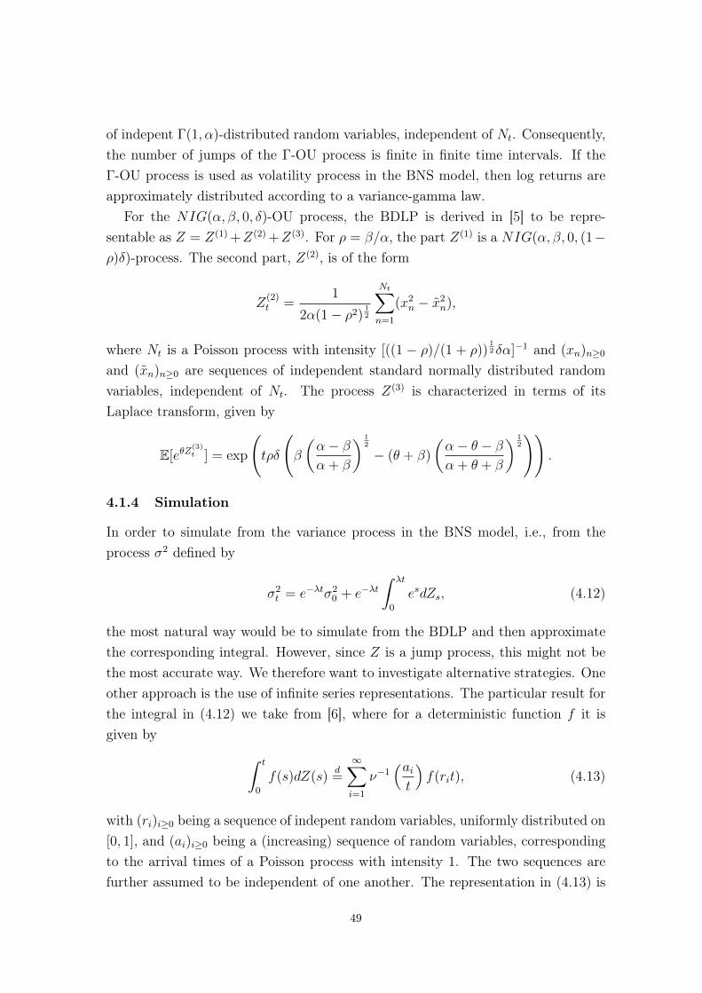
of indepent Γ(1, α)-distributed random variables, independent of Nt. Consequently,the number of jumps of the Γ-OU process is finite in finite time intervals. If theΓ-OU process is used as volatility process in the BNS model, then log returns areapproximately distributed according to a variance-gamma law.

For the NIG(α, β, 0, δ)-OU process, the BDLP is derived in [5] to be repre-sentable as Z = Z(1) +Z(2) +Z(3). For ρ = β/α, the part Z(1) is a NIG(α, β, 0, (1−ρ)δ)-process. The second part, Z(2), is of the form

Z(2)t =

1

2α(1− ρ2)12

Nt∑n=1

(x2n − x2

n),

where Nt is a Poisson process with intensity [((1 − ρ)/(1 + ρ))12 δα]−1 and (xn)n≥0

and (xn)n≥0 are sequences of independent standard normally distributed randomvariables, independent of Nt. The process Z(3) is characterized in terms of itsLaplace transform, given by

E[eθZ(3)t ] = exp

(tρδ

(β

(α− βα + β

) 12

− (θ + β)

(α− θ − βα + θ + β

) 12

)).

4.1.4 Simulation

In order to simulate from the variance process in the BNS model, i.e., from theprocess σ2 defined by

σ2t = e−λtσ2

0 + e−λt∫ λt

0

esdZs, (4.12)

the most natural way would be to simulate from the BDLP and then approximatethe corresponding integral. However, since Z is a jump process, this might not bethe most accurate way. We therefore want to investigate alternative strategies. Oneother approach is the use of infinite series representations. The particular result forthe integral in (4.12) we take from [6], where for a deterministic function f it isgiven by ∫ t

0

f(s)dZ(s)d=∞∑i=1

ν−1(ait

)f(rit), (4.13)

with (ri)i≥0 being a sequence of indepent random variables, uniformly distributed on[0, 1], and (ai)i≥0 being a (increasing) sequence of random variables, correspondingto the arrival times of a Poisson process with intensity 1. The two sequences arefurther assumed to be independent of one another. The representation in (4.13) is

49

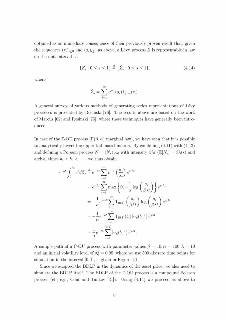
obtained as an immediate consequence of their previously proven result that, giventhe sequences (ri)i≥0 and (ai)i≥0 as above, a Lévy process Z is representable in lawon the unit interval as

Zs : 0 ≤ s ≤ 1 d= Zs : 0 ≤ s ≤ 1, (4.14)

where

Zs =∞∑i=1

ν−1(ai)1[0,s](ri).

A general survey of various methods of generating series representations of Lévyprocesses is presented by Rosiński [76]. The results above are based on the workof Marcus [62] and Rosiński [75], where these techniques have generally been intro-duced.

In case of the Γ-OU process (Γ(β, α) marginal law), we have seen that it is possibleto analytically invert the upper tail mass function. By combining (4.11) with (4.13)and defining a Poisson process N = (Ns)s≥0 with intensity βλt (E[Ns] = βλts) andarrival times b1 < b2 < . . . , we thus obtain

e−λt∫ λt

0

esdZsd= e−λt

∞∑i=1

ν−1( aiλt

)eriλt

= e−λt∞∑i=1

max

0,− 1

αlog

(aiβλt

)eriλt

= − 1

αe−λt

∞∑i=1

1(0,1)

(aiβλt

)log

(aiβλt

)eriλt

= +1

αe−λt

∞∑i=1

1(0,1)(bi) log(b−1i )eriλt

=1

αe−λt

N(1)∑i=1

log(b−1i )eriλt.

A sample path of a Γ-OU process with parameter values β = 10, α = 100, λ = 10

and an initial volatility level of σ20 = 0.08, where we use 500 discrete time points for

simulation in the interval [0, 1], is given in Figure 4.1.Since we adopted the BDLP in the dynamics of the asset price, we also need to

simulate the BDLP itself. The BDLP of the Γ-OU process is a compound Poissonprocess (cf., e.g., Cont and Tankov [31]). Using (4.14) we proceed as above to

50

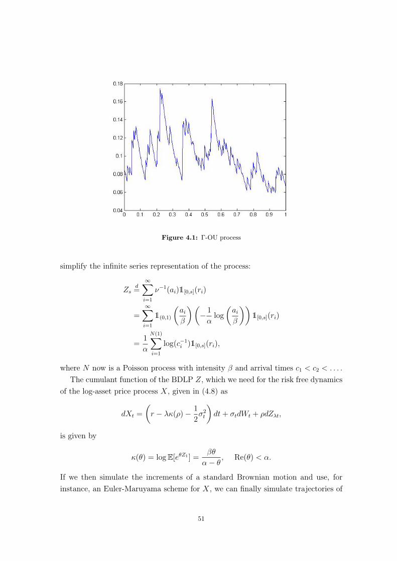
Figure 4.1: Γ-OU process

simplify the infinite series representation of the process:

Zsd=∞∑i=1

ν−1(ai)1[0,s](ri)

=∞∑i=1

1(0,1)

(aiβ

)(− 1

αlog

(aiβ

))1[0,s](ri)

=1

α

N(1)∑i=1

log(c−1i )1[0,s](ri),

where N now is a Poisson process with intensity β and arrival times c1 < c2 < . . . .The cumulant function of the BDLP Z, which we need for the risk free dynamics

of the log-asset price process X, given in (4.8) as

dXt =

(r − λκ(ρ)− 1

2σ2t

)dt+ σtdWt + ρdZλt,

is given by

κ(θ) = logE[eθZ1 ] =βθ

α− θ, Re(θ) < α.

If we then simulate the increments of a standard Brownian motion and use, forinstance, an Euler-Maruyama scheme for X, we can finally simulate trajectories of

51

the asset price.A sample path simulated with this strategy, together with the volatility process

and its BDLP, is given in Figure 4.2. We use the parameter values from [68],where the Γ-OU BNS model is calibrated to a data set of Call Options on the S&P500 index. Their obtained values are β = 1.0071, α = 116.01, λ = 1.6787, ρ =

−4.4617, σ20 = 0.0658832. Further, we take a risk free interest rate of r = 0.5538%,

an initial asset price of S0 = 100, and use 500 time steps of size 0.002 for simulationin the interval [0, 1].

Figure 4.2: Γ-OU BNS model

For the IG-OU process, the series in (4.13) converges slowly, since the decay ofν−1(x) for x → ∞ is only of quadratic order in this case (cf. [6]). A more efficientway to simulate from the IG-OU process has thus been suggested by Valdivieso,Schoutens, and Tuerlinckx [83], who make use of a special path rejection technique.Based on the decomposition of the BDLP given above, that is into an IG-processand a compound Poisson process as in (4.10), and using an Euler discretizationscheme, they derive the following recursive scheme for simulation of an IG(δ, γ)-

52

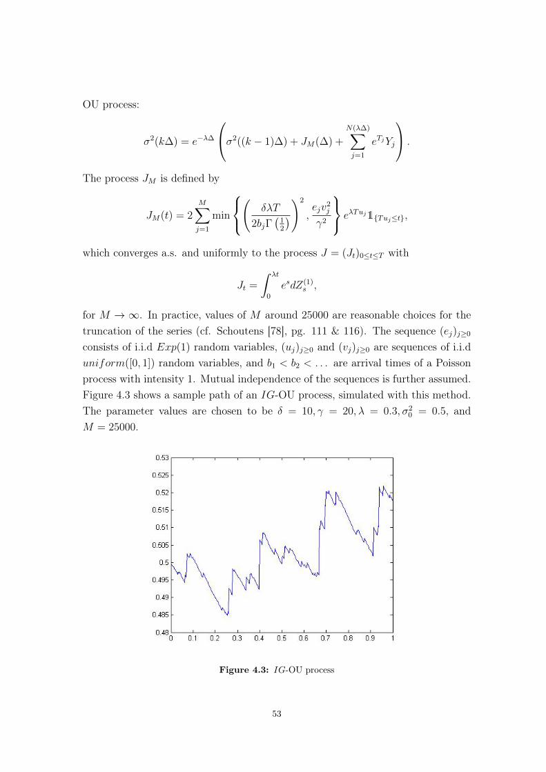
OU process:

σ2(k∆) = e−λ∆

σ2((k − 1)∆) + JM(∆) +

N(λ∆)∑j=1

eTjYj

.

The process JM is defined by

JM(t) = 2M∑j=1

min

(

δλT

2bjΓ(

12

))2

,ejv

2j

γ2

eλTuj1Tuj≤t,

which converges a.s. and uniformly to the process J = (Jt)0≤t≤T with

Jt =

∫ λt

0

esdZ(1)s ,

for M → ∞. In practice, values of M around 25000 are reasonable choices for thetruncation of the series (cf. Schoutens [78], pg. 111 & 116). The sequence (ej)j≥0

consists of i.i.d Exp(1) random variables, (uj)j≥0 and (vj)j≥0 are sequences of i.i.duniform([0, 1]) random variables, and b1 < b2 < . . . are arrival times of a Poissonprocess with intensity 1. Mutual independence of the sequences is further assumed.Figure 4.3 shows a sample path of an IG-OU process, simulated with this method.The parameter values are chosen to be δ = 10, γ = 20, λ = 0.3, σ2

0 = 0.5, andM = 25000.

Figure 4.3: IG-OU process

53

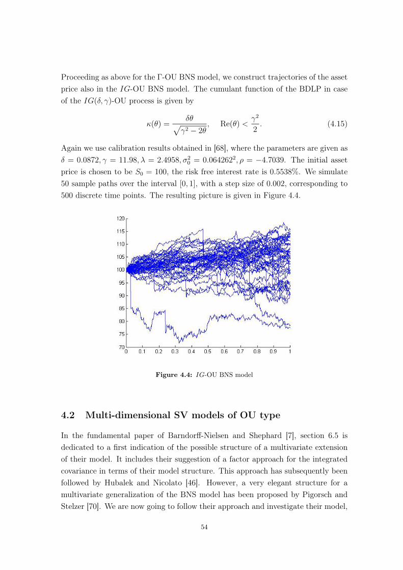
Proceeding as above for the Γ-OU BNS model, we construct trajectories of the assetprice also in the IG-OU BNS model. The cumulant function of the BDLP in caseof the IG(δ, γ)-OU process is given by

κ(θ) =δθ√γ2 − 2θ

, Re(θ) <γ2

2. (4.15)

Again we use calibration results obtained in [68], where the parameters are given asδ = 0.0872, γ = 11.98, λ = 2.4958, σ2

0 = 0.0642622, ρ = −4.7039. The initial assetprice is chosen to be S0 = 100, the risk free interest rate is 0.5538%. We simulate50 sample paths over the interval [0, 1], with a step size of 0.002, corresponding to500 discrete time points. The resulting picture is given in Figure 4.4.

Figure 4.4: IG-OU BNS model

4.2 Multi-dimensional SV models of OU type

In the fundamental paper of Barndorff-Nielsen and Shephard [7], section 6.5 isdedicated to a first indication of the possible structure of a multivariate extensionof their model. It includes their suggestion of a factor approach for the integratedcovariance in terms of their model structure. This approach has subsequently beenfollowed by Hubalek and Nicolato [46]. However, a very elegant structure for amultivariate generalization of the BNS model has been proposed by Pigorsch andStelzer [70]. We are now going to follow their approach and investigate their model,

54

particularly in the context of (Spread) Option pricing, in the remainder of thisthesis.

An even more general set-up, namely the supOU Stochastic Volatility model,has been introduced in Barndorff-Nielsen and Stelzer [12]. This model is basedon describing the volatility by a positive semidefinite supOU process, as definedand studied in Barndorff-Nielsen and Stelzer [11] as a multivariate extension of thetheory of superpositions of univariate OU processes, which have been introducedin Barndorff-Nielsen [9]. The property, which makes the supOU model appealingfor financial modelling, is its feature of producing long-range dependence effects inthe volatility and in logarithmic returns. This behaviour, which is usually observedin financial return data, cannot be reproduced by the model, which uses only onepositive semidefinite OU type process. Furthermore, in [12] a discussion of thepossibility of factor modelling within their framework is included and the model ofHubalek and Nicolato [46] is finally explained to be a special case thereof.

4.2.1 Notation

We mainly adopt the notation used in [8]. By Mm,n(K) we denote the set of allK-valued (m× n)-matrices. We abbreviatory write Mn in case m = n and K = R.We denote the subspace of Mn of all symmetric matrices by Sn, the cone of allposititve semidefinite symmetric matrices by S+

n , and the open cone of all positivedefinite symmetric matrices by S++

n . For the identity matrix in Rn×n we write In.σ(·) denotes the spectrum of an operator, being the set of eigenvalues for a matrixA ∈Mn(R).

The addition of two sets A,B ⊆ R is defined by A+B := a+ b : a ∈ A, b ∈ B.The Kronecker product of two matrices A ∈ Mm,n, B ∈ Mp,r is denoted by A⊗ B.It is defined as the matrix C, where Cij = aij · B, i.e., every element of A ismultiplied by the matrix B. This means that C ∈ Mmp,nr. Further, 〈x, y〉 := x>y,being the Euclidean scalar product on Rn. On Mn(R) we use the scalar product〈A,B〉 := tr(A>B) and on Rn×Mn we define 〈(x1, Y1), (x2, Y2)〉 := x>1 x2+tr(Y >1 Y2).We use the superscript asterisk to indicate adjoints of operators or matrices. For alinear operator A : V → W , where V,W are vector spaces, the adjoint operator A∗

is the unique linear operator such that 〈Ax, y〉W = 〈x,A∗y〉V for all x ∈ V, y ∈ W .For a matrix A ∈ Mm,n(C), one gets the adjoint matrix A∗ by taking the complexconjugate of each entry and transposing the matrix.

Let X, Y be two stochastic processes with values in Md,m and Mn,p, respectively.Let L be an Mm,n-valued semimartingale. Then

∫ t0XtdLtYt stands for the (d × p)

55

random matrix, where the element in the i-th row and j-th column is given by∑mk=1

∑nl=1

∫ t0X iks Y

ljs dL

kls .

4.2.2 The general multi-dimensional OU type SV model

As already mentioned above, the model we deal with has in principle been intro-duced by Pigorsch and Stelzer [70]. However, they define the model with jumpsonly occurring in the volatility process. We want to formulate the model in thesense of Muhle-Karbe, Pfaffel, and Stelzer [66], who also include a jump componentin the asset price process itself, in order to make allowance for a leverage effect inthe model.

Aiming for the model formulation, we first address some of the theory, where themodel is based on. The crucial point of the model is the use of matrix subordinatorsfor the construction of the volatiliy process. The concept of matrix subordinatorshas first been considered in Barndorff-Nielsen and Pérez-Abreu [10].

Definition 4.1: An Sd-valued Lévy process L = (Lt)t∈R+ is called matrix subordi-nator, if for its increments it holds that Lt − Ls ∈ S+

d a.s. for all t ≥ s.

For a matrix subordinator L, we consider the characteristic function φL1(Z) =

E[ei tr(ZL1)], where Z ∈Md(R). In terms of the Lévy-Khintchine representation, thecharacteristic exponent is of the form

ψL(Z) = i tr(γLZ) +

∫S+d

(ei tr(XZ) − 1)κL(dX),

with a drift matrix γL ∈ S+d and a Lévy measure κL on Sd, which satisfies the

conditions κL(Sd\S+d ) = 0 and

∫‖X‖≤1 ‖X‖κL(dX) <∞.

We also consider the cumulant transform ΘL, which is, for Z ∈ Md(C), definedby

ΘL(Z) = ψL(−iZ) = tr(γLZ) +

∫S+d

(etr(XZ) − 1)κL(dX).

Analogously to the univariate BNS model, the volatility process will be definedas a process of Ornstein-Uhlenbeck type. However, in the multivariate case we aredealing with matrix-valued OU type processes. Such processes have been introducedby Barndorff-Nielsen and Stelzer [8], in the light of the general study of processesof finite variation, which take values in the space of positive semidefinite matrices.

The crucial idea of generalising OU processes to matrix valued processes, is toidentify Md(R) with Rd2 . In this context, we will use a vectorisation operator

56

denoted by vec: Md(R) → Rd2 , which is the bijective linear operator that stacksthe columns of a matrix below one another.

Definition 4.2: Let L = (Lt)t∈R be a Lévy process with values in Md(R) and letA : Md(R)→Md(R) be a linear operator. A solution of the SDE

dXt = AXtdt+ dLt (4.16)

is called a (matrix-valued) process of Ornstein-Uhlenbeck type.

For some given value X0, it can be shown that (4.16) has a unique solution, whichis - analoguesly to the univariate case - given by

Xt = eAtX0 +

∫ t

0

eA(t−s)dLs.

Moreover, the two conditions E[log+ ‖L1‖] <∞ and σ(A) ∈ (−∞, 0)+iR guaranteethat the unique stationary solution of (4.16) is given by

Xt =

∫ t

−∞eA(t−s)dLs.

With the intention of constructing a process, which is suitable for modelling thestochastic evolution of a covariance matrix, we are interested in positive semidef-inite Ornstein-Uhlenbeck processes. Therefore, we need to make use of matrixsubordinators as driving Lévy processes. Then, for an initial matrix X0 ∈ S+

d andfor a linear operator A, which satisifies the condition eAt(S+

d ) ⊆ S+d for all t ∈ R+,

(Xt)t∈R+ only takes values in S+d . In other words, the condition on A means that

we are now searching for linear operators A such that the exponential operator eAt

preserves positive semidefiniteness for all t ∈ R+. A sufficient condition for ensuringthis is given in [8] (Proposition 4.4), as follows:

Proposition 4.1: Assume the operator A : Md(R) → Md(R) is representable asX 7→ AX + XA∗ for some A ∈ Md(R). Then eAt has the representation X 7→eAtXeA

∗t and eAt(S+d ) = S+

d for all t ∈ R.

Remark: The operator A associated with the matrix A can be represented as

vec−1 ((A⊗ I) + (I ⊗ A)) vec .

The above results are combined in the subsequent theorem, which will in furtherconsequence enable us to formulate the model.

57

Theorem 4.4: Let L = (Lt)t∈R be a matrix subordinator satisfying E[log+ ‖L1‖] <∞ and A ∈ Md such that σ(A) ⊂ (−∞, 0) + iR. Then the stochastic differentialequation of Ornstein-Uhlenbeck type

dXt = (AXt +XtA∗)dt+ dLt (4.17)

has a unique stationary solution, given by

Xt =

∫ t

−∞eA(t−s)dLse

A∗(t−s).

Moreover, Xt ∈ S+d for all t ∈ R. For a given initial value X0, the unique strong

solution of (4.17) satisfies

Xt = eAtX0eA∗t +

∫ t

0

eA(t−s)dLseA∗(t−s).

Remark: Applying the vectorization operator on Xt, we get the representation

vec(Xt) =

∫ t

−∞e(Id⊗A+A⊗Id)(t−s)d vec(Ls).

Equipped with the theory introduced above, we are now able to formulate themodel along the lines of Muhle-Karbe, Pfaffel, and Stelzer [66]. Let L be a ma-trix subordinator and let W be a Rd-valued Brownian motion, independent of L.The multivariate stochastic volatility model of OU type is defined via the followingdynamics of the logarithmic asset returns and the volatility, respectively:

dYt = (µ+ β(Σt))dt+ Σ12t dWt + ρ(dLt), (4.18)

dΣt = (AΣt + ΣtA>)dt+ dLt, (4.19)

with initial values Y0 ∈ Rd, Σ0 ∈ S+d , and parameters µ ∈ Rd and A ∈ Md(R)

such that 0 /∈ σ(A) + σ(A). The risk premium and the leverage term are modeledusing the linear operators β, ρ : Md(R) → Rd. A common way of specifying theseoperators is to choose coefficients β1, . . . , βd ∈ R and ρ1, . . . , ρd ∈ R for the diagonalelements of the argument, i.e.,

β(X) =

β1X11

...βdXdd

, ρ(X) =

ρ1X11

...ρdXdd

, ∀X ∈Md(R).

In this case, we call β and ρ diagonal. If β and ρ are taken to be diagonal and

58

also A is chosen as a diagonal matrix, then the model for each asset is equivalentin distribution to a univariate BNS model.

Since, in the formulation of the model, the square root of a positive semidefinite OUprocess is used, we want to mention a general result for such square root processes,in order to explicitly address its unique existence and finite variation property. Thisresult is due to Barndorff-Nielsen and Stelzer [8] (Proposition 6.7).

Proposition 4.2: Let (Xt)t∈R+ be an S+d -valued process of Ornstein-Uhlenbeck type

driven by a matrix subordinator L with drift γ ∈ S+d and associated Poisson random

measure µ. Then the unique positive square root Yt =√Xt is of finite variation and

has the following representation:

dYt = X−1t− (AXt− +Xt−A

∗ + γ)dt+

∫S+d \0

(√Xt− + x−

√Xt−

)µ(dt, dx)

= Y−1t− (AY 2

t− + Y 2t−A

∗ + γ)dt+

∫S+d \0

(√Y 2t− + x− Yt−

)µ(dt, dx),

provided that the process Xt is locally bounded within S++d or the integrals∫ t

0

X−1s−(AXs− +Xs−A

∗ + γ)ds and∫ t

0

∫S+d \0

(√Xs− + x−

√Xs−

)µ(ds, dx)

exist a.s. for all t ∈ R. Here, Xt− is the linear operator Z 7→√Xt−Z + Z

√Xt−

and Yt− is the mapping Z 7→ Yt−Z + ZYt−.

Particularly the application of transform-based methods in the context of optionpricing, as we will do in chapter 5, requires the characteristic function of the assetprice. For the multivariate OU type SV model, we may use the following result,computed in [66] (Theorem 2.5).

Theorem 4.5: For every (y, z) ∈ Rd ×Md(R) and t ∈ R+, the joint characteristicfunction of (Yt,Σt) is given by

E[exp(i〈(y, z), (Yt,Σt)〉)]

= exp

iy>(Y0 + µt) + i tr(Σ0e

A>tzeAt)

+ i tr

(Σ0

(eA>tA−∗

(β∗(y) +

i

2yy>

)eAt −A−∗

(β∗(y) +

i

2yy>

)))+

∫ t

0

ψL

(eA>szeAs + ρ∗(y) + eA

>sA−∗(β∗(y) +

i

2yy>

)eAs −A−∗

(β∗(y) +

i

2yy>

))ds

,

where A−∗ := (A∗)−1 denotes the inverse of the adjoint of A : X 7→ AX + XA>,

59

that is, the inverse of A∗ : X 7→ A>X +XA.

In the remainder of this subsection, we want to study some theoretical propertiesof the model. All of the three subsequent results are due to [66]; the proofs can befound therein.

The first theorem deals with the regularity of the moment generating function.We will use this result in section 4.2.3, where we derive the moment generatingfunction for the concrete specification of the two-dimensional OU Wishart modelalong the lines of [66]. This will particularly enable us to apply the method intro-duced in section 2.1.3 in order to price Spread Options, what will be done withinthe context of our numerical investigations in chapter 5.

Theorem 4.6: Suppose the matrix subordinator L satisfies∫‖X‖≥1

etr(RX)κL(dX) <∞ for all R ∈Md(R) with ‖R‖ < ε,

for some ε > 0. Then the moment generating function ΦYt of Yt is analytic on theopen convex set

Sθ := y ∈ Cd : ‖Re(y)‖ < θ,

where

θ := − ‖ρ‖(e2‖A‖t + 1)‖A−1‖

− ‖β‖+√

∆ > 0

with

∆ :=

(‖ρ‖

(e2‖A‖t + 1)‖A−1‖+ ‖β‖

)2

+2ε

(e2‖A‖t + 1)‖A−1‖.

Moreover,

ΦYt(y) = exp

(y>(Y0 + µt) + tr(Σ0Hy(t)) +

∫ t

0

ΘL(Hy(s) + ρ∗(y))ds

)for all y ∈ Sθ, where

Hy(s) := eA>sA−∗

(β∗(y) +

1

2yy>

)eAs −A−∗

(β∗(y) +

1

2yy>

). (4.20)

In accordance with the Fundamental Theorem of Asset Pricing, we need to addressthe question of equivalent martingale measures. First, we study the conditionsunder which the discounted price process in the multivariate OU type SV model

60

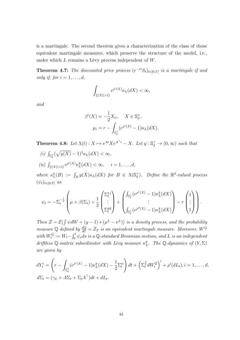
is a martingale. The second theorem gives a characterization of the class of thoseequivalent martingale measures, which preserve the structure of the model, i.e.,under which L remains a Lévy process independent of W .

Theorem 4.7: The discounted price process (e−rtSt)t∈[0,T ] is a martingale if andonly if, for i = 1, . . . , d, ∫

‖X‖>1eρi(X)κL(dX) <∞,

and

βi(X) = −1

2Xii, X ∈ S+

d ,

µi = r −∫S+d

(eρi(X) − 1)κL(dX).

Theorem 4.8: Let Λ(t) : X 7→ eAtXeA>t −X. Let y : S+

d → (0,∞) such that

(i)∫S+d

(√y(X)− 1)2κL(dX) <∞,

(ii)∫‖X‖>1 e

ρi(X)κyL(dX) <∞, i = 1, . . . , d,

where κyL(B) :=∫By(X)κL(dX) for B ∈ Λ(S+

d ). Define the Rd-valued process(ψt)t∈[0,T ] as

ψt = −Σ− 1

2t

µ+ β(Σt) +1

2

Σ11t...

Σddt

+

∫S+d

(eρ1(X) − 1)κyL(dX)

...∫S+d

(eρd(X) − 1)κyL(dX)

− r

1...1

.

Then Z = E(∫ψdW + (y − 1) ∗ (µL − νL)) is a density process, and the probability

measure Q defined by dQdP = ZT is an equivalent martingale measure. Moreover, WQ

withWQt := Wt−

∫ t0ψsds is a Q-standard Brownian motion, and L is an independent

driftless Q-matrix subordinator with Lévy measure κyL. The Q-dynamics of (Y,Σ)

are given by

dY it =

(r −

∫S+d

(eρi(X) − 1)κyL(dX)− 1

2Σiit

)dt+

(Σ

12t dW

Qt

)i+ ρi(dLt), i = 1, . . . , d,

dΣt = (γL + AΣt + ΣtA>)dt+ dLt.

61

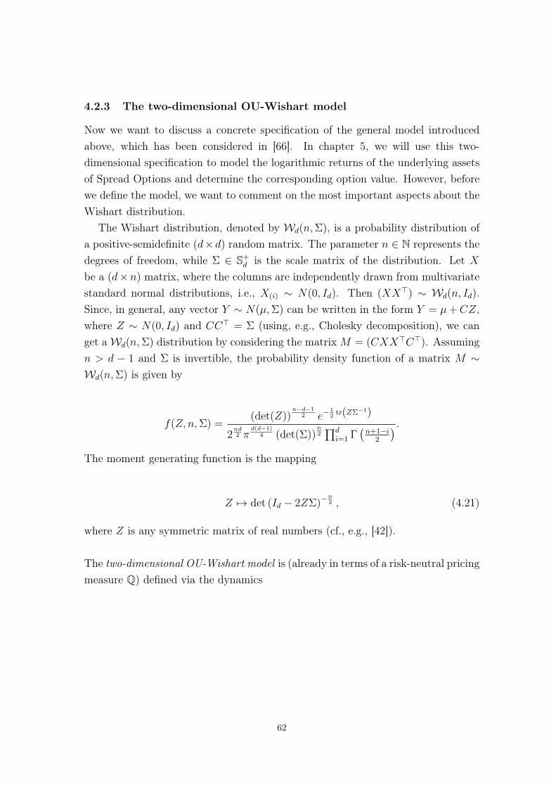
4.2.3 The two-dimensional OU-Wishart model

Now we want to discuss a concrete specification of the general model introducedabove, which has been considered in [66]. In chapter 5, we will use this two-dimensional specification to model the logarithmic returns of the underlying assetsof Spread Options and determine the corresponding option value. However, beforewe define the model, we want to comment on the most important aspects about theWishart distribution.

The Wishart distribution, denoted by Wd(n,Σ), is a probability distribution ofa positive-semidefinite (d×d) random matrix. The parameter n ∈ N represents thedegrees of freedom, while Σ ∈ S+

d is the scale matrix of the distribution. Let Xbe a (d×n) matrix, where the columns are independently drawn from multivariatestandard normal distributions, i.e., X(i) ∼ N(0, Id). Then (XX>) ∼ Wd(n, Id).Since, in general, any vector Y ∼ N(µ,Σ) can be written in the form Y = µ+CZ,where Z ∼ N(0, Id) and CC> = Σ (using, e.g., Cholesky decomposition), we canget aWd(n,Σ) distribution by considering the matrixM = (CXX>C>). Assumingn > d − 1 and Σ is invertible, the probability density function of a matrix M ∼Wd(n,Σ) is given by

f(Z, n,Σ) =(det(Z))

n−d−12 e−

12

tr(ZΣ−1)

2nd2 π

d(d−1)4 (det(Σ))

n2∏d

i=1 Γ(n+1−i

2

) .The moment generating function is the mapping

Z 7→ det (Id − 2ZΣ)−n2 , (4.21)

where Z is any symmetric matrix of real numbers (cf., e.g., [42]).

The two-dimensional OU-Wishart model is (already in terms of a risk-neutral pricingmeasure Q) defined via the dynamics

62

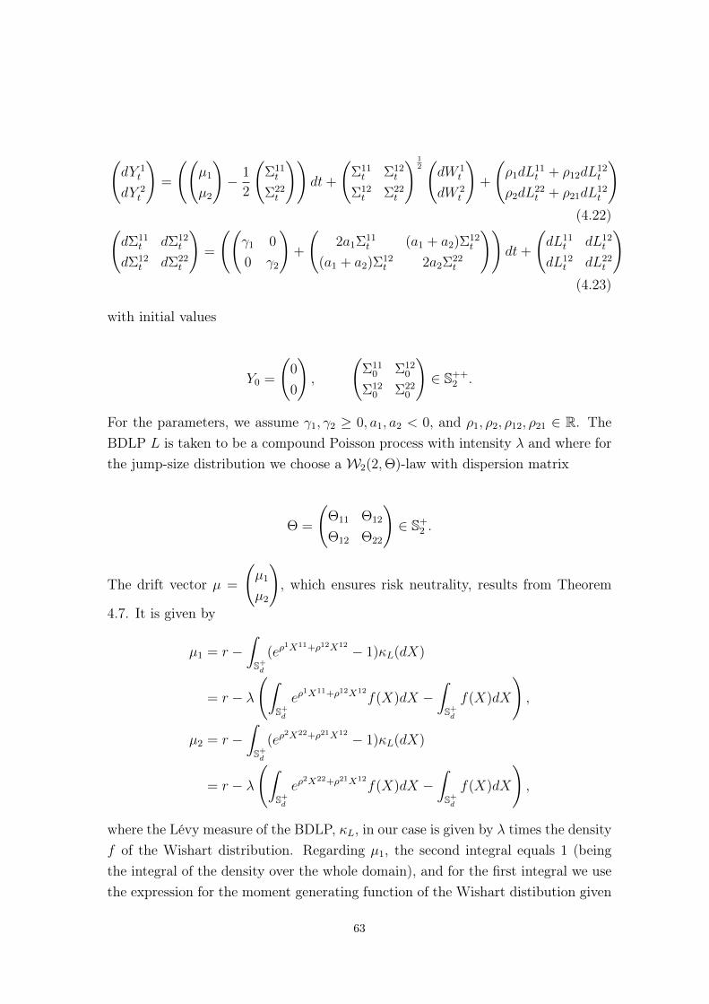
(dY 1

t

dY 2t

)=

((µ1

µ2

)− 1

2

(Σ11t

Σ22t

))dt+

(Σ11t Σ12

t

Σ12t Σ22

t

) 12(dW 1

t

dW 2t

)+

(ρ1dL

11t + ρ12dL

12t

ρ2dL22t + ρ21dL

12t

)(4.22)(

dΣ11t dΣ12

t

dΣ12t dΣ22

t

)=

((γ1 0

0 γ2

)+

(2a1Σ11

t (a1 + a2)Σ12t

(a1 + a2)Σ12t 2a2Σ22

t

))dt+

(dL11

t dL12t

dL12t dL22

t

)(4.23)

with initial values

Y0 =

(0

0

),

(Σ11

0 Σ120

Σ120 Σ22

0

)∈ S++

2 .

For the parameters, we assume γ1, γ2 ≥ 0, a1, a2 < 0, and ρ1, ρ2, ρ12, ρ21 ∈ R. TheBDLP L is taken to be a compound Poisson process with intensity λ and where forthe jump-size distribution we choose a W2(2,Θ)-law with dispersion matrix

Θ =

(Θ11 Θ12

Θ12 Θ22

)∈ S+

2 .

The drift vector µ =

(µ1

µ2

), which ensures risk neutrality, results from Theorem

4.7. It is given by

µ1 = r −∫S+d

(eρ1X11+ρ12X12 − 1)κL(dX)

= r − λ

(∫S+d

eρ1X11+ρ12X12

f(X)dX −∫S+d

f(X)dX

),

µ2 = r −∫S+d

(eρ2X22+ρ21X12 − 1)κL(dX)

= r − λ

(∫S+d

eρ2X22+ρ21X12

f(X)dX −∫S+d

f(X)dX

),

where the Lévy measure of the BDLP, κL, in our case is given by λ times the densityf of the Wishart distribution. Regarding µ1, the second integral equals 1 (beingthe integral of the density over the whole domain), and for the first integral we usethe expression for the moment generating function of the Wishart distibution given

63

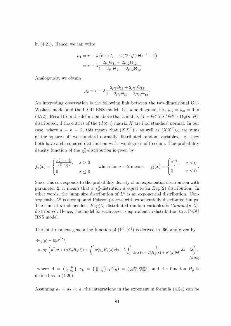
in (4.21). Hence, we can write

µ1 = r − λ(det (I2 − 2 ( ρ1 ρ120 0 ) Θ)−1 − 1

)= r − λ 2ρ1Θ11 + 2ρ12Θ12

1− 2ρ1Θ11 − 2ρ12Θ12

.

Analogously, we obtain

µ2 = r − λ 2ρ2Θ22 + 2ρ21Θ12

1− 2ρ2Θ22 − 2ρ21Θ12

.

An interesting observation is the following link between the two-dimensional OU-Wishart model and the Γ-OU BNS model. Let ρ be diagonal, i.e., ρ12 = ρ21 = 0 in(4.22). Recall from the definition above that a matrixM = Θ

12XX>Θ

12 isWd(n,Θ)-

distributed, if the entries of the (d× n) matrix X are i.i.d standard normal. In ourcase, where d = n = 2, this means that (XX>)11 as well as (XX>)22 are sumsof the squares of two standard normally distributed random variables, i.e., theyboth have a chi-squared distribution with two degrees of freedom. The probabilitydensity function of the χ2

n-distribution is given by

fn(x) =

xn2−1e−

x2

2n2 Γ(n

2), x > 0

0 x ≤ 0which for n = 2 means f2(x) =

e−x2

2, x > 0

0 x ≤ 0.

Since this corresponds to the probability density of an exponential distribution withparameter 2, it means that a χ2

2-distrution is equal to an Exp(2) distribution. Inother words, the jump size distribution of Lii is an exponential distribution. Con-sequently, Lii is a compound Poisson process with exponentially distributed jumps.The sum of n independent Exp(λ) distributed random variables is Gamma(n, λ)-distributed. Hence, the model for each asset is equivalent in distribution to a Γ-OUBNS model.

The joint moment generating function of (Y 1, Y 2) is derived in [66] and given by

ΦYt(y) = E[ey

>Yt ]

= exp

(y>µt+ tr(Σ0Hy(t)) +

∫ t

0

tr(γLHy(s))ds+ λ

∫ t

0

1

det(I2 − 2(Hy(s) + ρ∗(y))Θ)ds− λt

),

(4.24)

where A =(a1 00 a2

), γL =

(γ1 00 γ2

), ρ∗(y) = ( ρ1y1 ρ12y1

ρ21y2 ρ2y2 ) and the function Hy isdefined as in (4.20).

Assuming a1 = a2 =: a, the integrations in the exponent in formula (4.24) can be

64

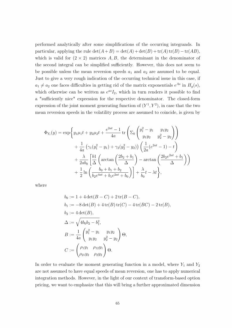
performed analytically after some simplifications of the occurring integrands. Inparticular, applying the rule det(A+B) = det(A) + det(B) + tr(A) tr(B)− tr(AB),which is valid for (2 × 2) matrices A,B, the determinant in the denominator ofthe second integral can be simplified sufficiently. However, this does not seem tobe possible unless the mean reversion speeds a1 and a2 are assumed to be equal.Just to give a very rough indication of the occurring technical issue in this case, ifa1 6= a2 one faces difficulties in getting rid of the matrix exponentials eAs in Hy(s),which otherwise can be written as easI2, which in turn renders it possible to finda "sufficiently nice" expression for the respective denominator. The closed-formexpression of the joint moment generating function of (Y 1, Y 2), in case that the twomean reversion speeds in the volatility process are assumed to coincide, is given by

ΦYt(y) = exp

y1µ1t+ y2µ2t+

e2at − 1

4atr

(Σ0

(y2

1 − y1 y1y2

y1y2 y22 − y2

))

+1

4a

(γ1(y2

1 − y1) + γ2(y22 − y2)

)( 1

2a(e2at − 1)− t

)+

λ

2ab0

[b1

∆

(arctan

(2b2 + b1

∆

)− arctan

(2b2e

2at + b1

∆

))+

1

2ln

(b0 + b1 + b2

b2e4at + b1e2at + b0

)]+λ

b0

t− λt,

where

b0 := 1 + 4 det(B − C) + 2 tr(B − C),

b1 := −8 det(B) + 4 tr(B) tr(C)− 4 tr(BC)− 2 tr(B),

b2 := 4 det(B),

∆ :=√

4b0b2 − b21,

B :=1

4a

(y2

1 − y1 y1y2

y1y2 y22 − y2

)Θ,

C :=

(ρ1y1 ρ12y1

ρ21y2 ρ2y2

)Θ.

In order to evaluate the moment generating function in a model, where Y1 and Y2

are not assumed to have equal speeds of mean reversion, one has to apply numericalintegration methods. However, in the light of our context of transform-based optionpricing, we want to emphasize that this will bring a further approximated dimension

65

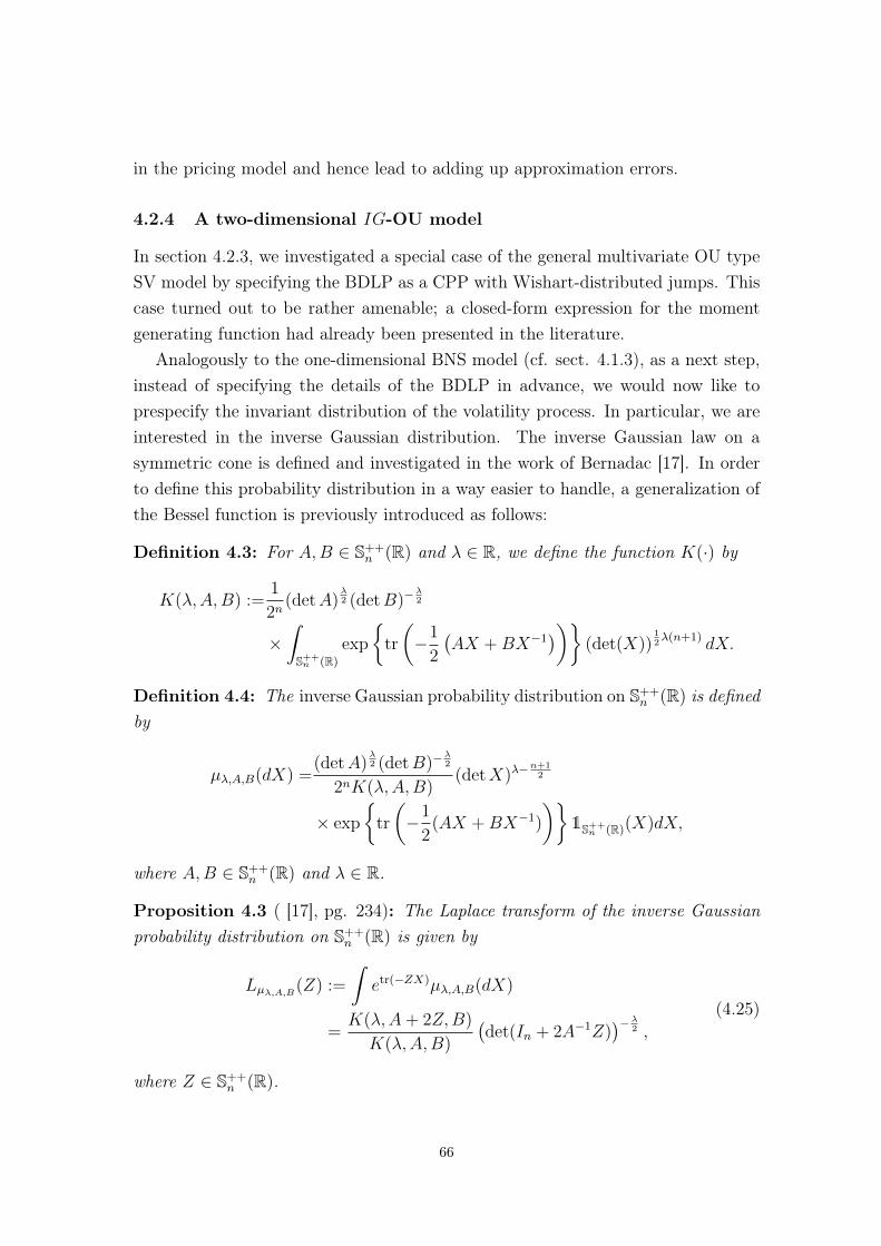
in the pricing model and hence lead to adding up approximation errors.

4.2.4 A two-dimensional IG-OU model

In section 4.2.3, we investigated a special case of the general multivariate OU typeSV model by specifying the BDLP as a CPP with Wishart-distributed jumps. Thiscase turned out to be rather amenable; a closed-form expression for the momentgenerating function had already been presented in the literature.

Analogously to the one-dimensional BNS model (cf. sect. 4.1.3), as a next step,instead of specifying the details of the BDLP in advance, we would now like toprespecify the invariant distribution of the volatility process. In particular, we areinterested in the inverse Gaussian distribution. The inverse Gaussian law on asymmetric cone is defined and investigated in the work of Bernadac [17]. In orderto define this probability distribution in a way easier to handle, a generalization ofthe Bessel function is previously introduced as follows:

Definition 4.3: For A,B ∈ S++n (R) and λ ∈ R, we define the function K(·) by

K(λ,A,B) :=1

2n(detA)

λ2 (detB)−

λ2

×∫S++n (R)

exp

tr

(−1

2

(AX +BX−1

))(det(X))

12λ(n+1) dX.

Definition 4.4: The inverse Gaussian probability distribution on S++n (R) is defined

by

µλ,A,B(dX) =(detA)

λ2 (detB)−

λ2

2nK(λ,A,B)(detX)λ−

n+12

× exp

tr

(−1

2(AX +BX−1)

)1S++

n (R)(X)dX,

where A,B ∈ S++n (R) and λ ∈ R.

Proposition 4.3 ( [17], pg. 234): The Laplace transform of the inverse Gaussianprobability distribution on S++

n (R) is given by

Lµλ,A,B(Z) :=

∫etr(−ZX)µλ,A,B(dX)

=K(λ,A+ 2Z,B)

K(λ,A,B)

(det(In + 2A−1Z)

)−λ2 ,

(4.25)

where Z ∈ S++n (R).

66

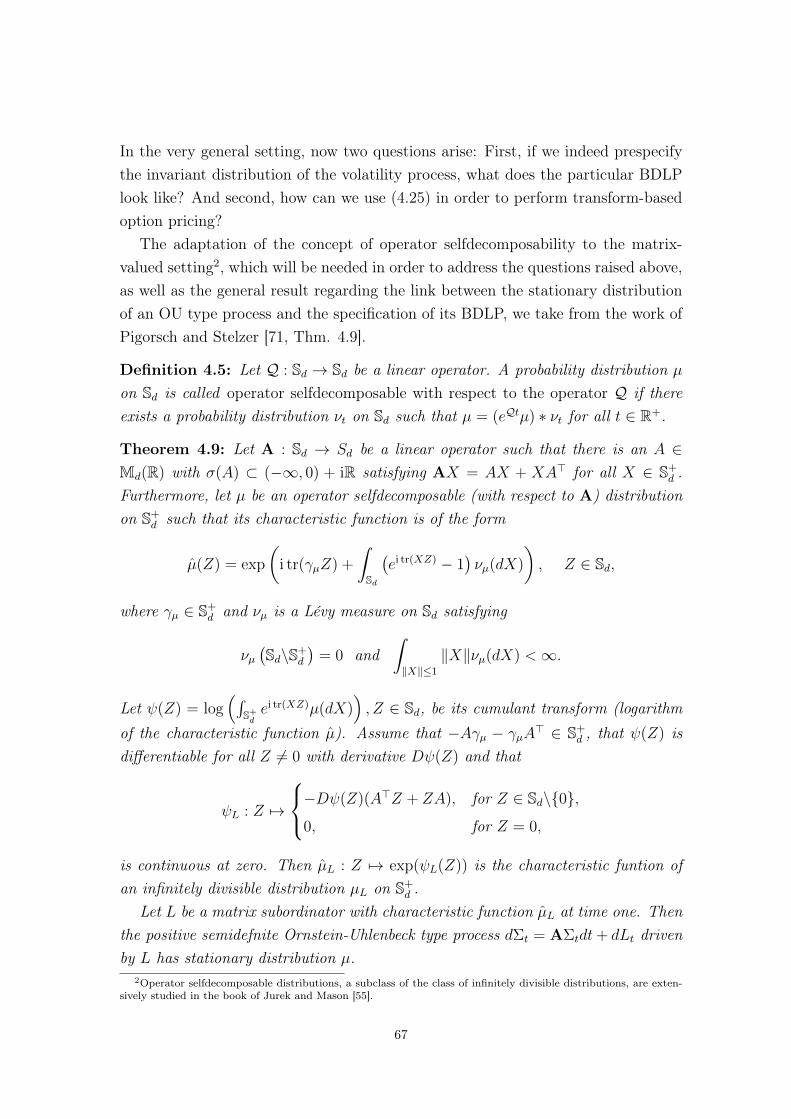
In the very general setting, now two questions arise: First, if we indeed prespecifythe invariant distribution of the volatility process, what does the particular BDLPlook like? And second, how can we use (4.25) in order to perform transform-basedoption pricing?

The adaptation of the concept of operator selfdecomposability to the matrix-valued setting2, which will be needed in order to address the questions raised above,as well as the general result regarding the link between the stationary distributionof an OU type process and the specification of its BDLP, we take from the work ofPigorsch and Stelzer [71, Thm. 4.9].

Definition 4.5: Let Q : Sd → Sd be a linear operator. A probability distribution µon Sd is called operator selfdecomposable with respect to the operator Q if thereexists a probability distribution νt on Sd such that µ = (eQtµ) ∗ νt for all t ∈ R+.

Theorem 4.9: Let A : Sd → Sd be a linear operator such that there is an A ∈Md(R) with σ(A) ⊂ (−∞, 0) + iR satisfying AX = AX + XA> for all X ∈ S+

d .Furthermore, let µ be an operator selfdecomposable (with respect to A) distributionon S+

d such that its characteristic function is of the form

µ(Z) = exp

(i tr(γµZ) +

∫Sd

(ei tr(XZ) − 1

)νµ(dX)

), Z ∈ Sd,

where γµ ∈ S+d and νµ is a Lévy measure on Sd satisfying

νµ(Sd\S+

d

)= 0 and

∫‖X‖≤1

‖X‖νµ(dX) <∞.

Let ψ(Z) = log(∫

S+dei tr(XZ)µ(dX)

), Z ∈ Sd, be its cumulant transform (logarithm

of the characteristic function µ). Assume that −Aγµ − γµA> ∈ S+d , that ψ(Z) is

differentiable for all Z 6= 0 with derivative Dψ(Z) and that

ψL : Z 7→

−Dψ(Z)(A>Z + ZA), for Z ∈ Sd\0,

0, for Z = 0,

is continuous at zero. Then µL : Z 7→ exp(ψL(Z)) is the characteristic funtion ofan infinitely divisible distribution µL on S+

d .Let L be a matrix subordinator with characteristic function µL at time one. Then

the positive semidefnite Ornstein-Uhlenbeck type process dΣt = AΣtdt+ dLt drivenby L has stationary distribution µ.

2Operator selfdecomposable distributions, a subclass of the class of infinitely divisible distributions, are exten-sively studied in the book of Jurek and Mason [55].

67

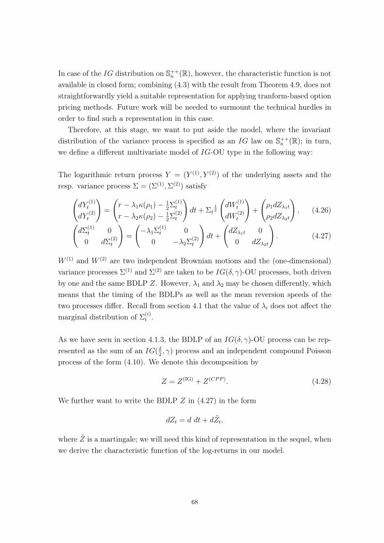
In case of the IG distribution on S++n (R), however, the characteristic function is not

available in closed form; combining (4.3) with the result from Theorem 4.9, does notstraightforwardly yield a suitable representation for applying tranform-based optionpricing methods. Future work will be needed to surmount the technical hurdles inorder to find such a representation in this case.

Therefore, at this stage, we want to put aside the model, where the invariantdistribution of the variance process is specified as an IG law on S++

n (R); in turn,we define a different multivariate model of IG-OU type in the following way:

The logarithmic return process Y = (Y (1), Y (2)) of the underlying assets and theresp. variance process Σ = (Σ(1),Σ(2)) satisfy(

dY(1)t

dY(2)t

)=

(r − λ1κ(ρ1)− 1

2Σ

(1)t

r − λ2κ(ρ2)− 12Σ

(2)t

)dt+ Σt

12

(dW

(1)t

dW(2)t

)+

(ρ1dZλ1t

ρ2dZλ2t

), (4.26)(

dΣ(1)t 0

0 dΣ(2)t

)=

(−λ1Σ

(1)t 0

0 −λ2Σ(2)t

)dt+

(dZλ1t 0

0 dZλ2t

). (4.27)

W (1) and W (2) are two independent Brownian motions and the (one-dimensional)variance processes Σ(1) and Σ(2) are taken to be IG(δ, γ)-OU processes, both drivenby one and the same BDLP Z. However, λ1 and λ2 may be chosen differently, whichmeans that the timing of the BDLPs as well as the mean reversion speeds of thetwo processes differ. Recall from section 4.1 that the value of λi does not affect themarginal distribution of Σ

(i)t .

As we have seen in section 4.1.3, the BDLP of an IG(δ, γ)-OU process can be rep-resented as the sum of an IG( δ

2, γ) process and an independent compound Poisson

process of the form (4.10). We denote this decomposition by

Z = Z(IG) + Z(CPP ). (4.28)

We further want to write the BDLP Z in (4.27) in the form

dZt = d dt+ dZt,

where Z is a martingale; we will need this kind of representation in the sequel, whenwe derive the characteristic function of the log-returns in our model.

68

A Lévy process L has the decomposition

Lt =

∫ t

0

∫ ∞0

zν(dz)dt+

∫ t

0

∫ ∞0

z (N(dz, dt)− ν(dz)dt) , (4.29)

where the second integral on the right-hand side is a martingale. In this representa-tion, N denotes a Poisson random measure and ν is the Lévy measure of L. Looselyspeaking, in (4.29) we split the process by writing its compensated version as onepart and its expectation as a separate second part.

Let us first have a look at the part Z(IG) in (4.28): The Lévy measure of an IG(a, b)

process is given by

ν(dx) =a√2πx−

32 e−

12b2x1x>0dx,

and the corresponding integral ∫ ∞0

zν(dz) =a

b.

Consequently, we get from (4.29) that, for i = 1, 2, we can write

dZ(IG)λit

=λiδ

2γdt+ dZ

(IG)λit

, (4.30)

where Z(IG) is a martingale.

For a compound Poisson process, the Lévy measure is given by

ν(dz) = θf(z)dz,

where θ denotes the intensity of the corresponding Poisson process and f denotes thedensity of the jump-size distribution. In our case (see section 4.1.3), the intensityof Z(CPP) is given by δγ

2, and the jumps, being squares of independent standard

normally distributed random variables, each follow a chi-squared distribution withone degree of freedom. The expected value of a chi-squared distributed randomvariable is its degree of freedom. Hence,∫ ∞

0

zν(dz) =1

γ

δγ

2=δ

2,

69

and, for i = 1, 2, we get the representation

dZ(CPP)λit

=λiδ

2dt+ Z

(CPP)λit

, (4.31)

with a martingale Z(CPP).

Combining (4.30) and (4.31), we can now write

dZλ1t =λ1δ

2γ(1 + γ) dt+ dZλ1t,

dZλ2t =λ1δ

2γ(1 + γ) dt+ dZλ2t,

where Z = Z(IG) + Z(CPP) is a martingale. We adopt this notation in the definitionof the model and reformulate it as follows:

dY(1)t =

(r − λ1κ(ρ1)− 1

2Σ

(1)t

)dt+

√Σ

(1)t dW

(1)t + ρ1dZλ1t,

dY(2)t =

(r − λ2κ(ρ2)− 1

2Σ

(2)t

)dt+

√Σ

(2)t dW

(2)t + ρ2dZλ2t,

dΣ(1)t =

(−λ1Σ

(1)t +

λ1δ

2γ(1 + γ)

)dt+ dZλ1t,

dΣ(2)t =

(−λ2Σ

(2)t +

λ2δ

2γ(1 + γ)

)dt+ dZλ2t.

(4.32)

Remark: From an economic point of view, this model can be advocated in the sensethat it should be interpreted as offering two assets whose usual fluctuations behavedifferently, but which are both affected by the same shocks in the market.

Remark: In (4.32) we have given the dynamics of all the individual processes ofthe model. However, when we initially formulate this model in (4.26) and (4.27),we have deliberately written also the volatility process in matrix notation (even ifthe non-diagonal elements are zero), in order to emphasize that this model shouldstill be seen as a special case of the general multivariate OU type SV model (4.18)- (4.19), and thus inherits all the properties derived in the general setting.

Now that we have formulated the model and we set about deriving the joint char-acteristic function of (Y (1), Y (2)), we want to exploit that the model is an affinestochastic volatility model in the sense of Keller-Ressel [56]. In order to add clarityand due to the general importance of affine models in mathematical finance, at thisstage, we want to undertake at least a very short excursus in the theory of affinemodels.

70

We start with the class of affine processes, which has originally been definedby Duffie, Filipović, and Schachermayer [40, Def. 2.1] in terms of a rather generalformulation, using, for a state space D, the semigroup (Pt)t≥0 of operators appliedto functions f in the set of bounded Borel-measurable functions bB(D), which canbe associated to a time-homogeneous Markov process X = (Xt)t≥0, by setting

Ptf(x) = E[f(Xt)|Xt = x], ∀x ∈ D.

We want to use a slightly modified formulation of this definition according to [56],since it fits better in the present context. Compared with the original definitionin [40], here stochastic continuity is already part of the definition.

Definition 4.6: Let X = (Xt,Px)t≥0,x∈D be a stochastically continuous, time-homogeneous Markov process with state space D = Rm

+ × Rn and where Px de-notes the distribution of X with initial value x, i.e., X0 = x, Px-almost surely.Then X is called an affine process, if its characteristic function is an exponentially-affine function of the state vector. This means that on iRd there exist functionsφ : R+ × iRd → C and ψ : R+ × iRd → Cd such that

Ex[e〈Xt,u〉

]= eφ(t,u)+〈x,ψ(t,u)〉,

for all x ∈ D, and for all (t, u) ∈ R+ × iRd.

A Stochastic Volatility model with asset price process X = (Xt)0≤t≤T and volatilityprocess V = (Vt)0≤t≤T is then called an affine Stochastic Volatility model, if thejoint process (X, V ) satisfies the following two assumptions:

(i) (X, V ) is a stochastically continuous, time-homogeneous Markov process.

(ii) The moment generating function Φt(u,w) of (Xt, Vt) is of particular affineform: There exist functions C(t, u, w) and D(t, u, w) such that

Φt(u,w) := E[exp(uXt + wVt)|X0, V0] = euX0+C(t,u,w)+V0D(t,u,w).

The functions C(·) and D(·) can be obtained as solutions of a system of ordinarydifferential equations of the (generalized) Riccati type.

It is shown in [56] that the one-dimensional BNS model belongs to this class. Themultivariate generalization of the BNS model is explained to be an affine stochasticvolatility model in the work of Cuchiero, Filipović, Mayerhofer, and Teichmann [34],which is dedicated to affine processes on positive semidefinite matrices. Moreover,almost all other relevant stochastic volatility models in the literature, as, e.g., the

71

models of Heston and Bates (see sect. 3.3.2), fall in the class of affine stochasticvolatility models (cf. [56]), as well as popular term structure models are usually ofthe affine type (cf. Cuchiero, Filipović and Teichmann [35]). In general, it can besaid that an affine structure of a model offers plenty of analytic tractability andstatistical flexibility; due to this fact, these kind of models are predominantly usedin the finance literature.

Let us now get back to our model. Equipped with the knowledge of the theorymentioned above, in order to derive the joint characteristic function of (Y (1), Y (2))

from (4.32), we define

f(~y,~v, t, ~u) := φYT |Ft(~u) = EQ [ei~uYT | ~y = Yt, ~v = Σt

]= ei~u~y+C(T−t)+~v ~D(T−t). (4.33)

We use the notation with arrows on top to emphasize vectors here. We want toapply Ito’s Lemma on (4.33), so we first have a look at all the quadratic covariationsbetween the occuring processes (recall that quadratic covariation is symmetric):

d[y(1), y(1)] = Σ(1)t dt+ ρ2

1d[Z]λ1t,

d[y(2), y(2)] = Σ(2)t dt+ ρ2

2d[Z]λ2t,

d[y(1), y(2)] = 0,

d[v(1), v(1)] = d[Z]λ1t,

d[v(2), v(2)] = d[Z]λ2t,

d[v(1), v(2)] = 0,

d[y(1), v(1)] = ρ1d[Z, Z]λ1t,

d[y(2), v(2)] = ρ2d[Z, Z]λ2t,

d[y(1), v(2)] = 0,

d[y(2), v(1)] = 0.

72

Ito’s Lemma then yields

df =∂f

∂tdt+

∂f

∂y(1)

((r − λ1κ(ρ1)− 1

2v(1))dt+

√v(1)dW

(1)t + ρ1dZλ1t

)+

∂f

∂y(2)

((r − λ2κ(ρ2)− 1

2v(2))dt+

√v(2)dW

(2)t + ρ2dZλ2t

)+

∂f

∂v(1)

((−λ1v

(1) +λ1δ

2γ(1 + γ)

)dt+ dZλ1t

)+

∂f

∂v(2)

((−λ2v

(2) +λ2δ

2γ(1 + γ)

)dt+ dZλ2t

)+

1

2

∂2f

∂y(1)2

(v(1)dt+ ρ2

1d[Z]λ1t)

+1

2

∂2f

∂y(2)2

(v(2)dt+ ρ2

2d[Z]λ2t)

+1

22

∂2f

∂y(1)∂y(2)· 0

+1

2

∂2f

∂v(1)2d[Z]λ1t +1

2

∂2f

∂v(2)2d[Z]λ2t

+1

22

∂2f

∂y(1)∂v(1)ρ1d[Z, Z]λ1t +

1

22

∂2f

∂y(2)∂v(2)ρ2d[Z, Z]λ2t,

and, setting the drift term equal to zero, we obtain

0 =∂f

∂t+

∂f

∂y(1)

(r − λ1κ(ρ1)− 1

2v(1))

+∂f

∂y(2)

(r − λ2κ(ρ2)− 1

2v(2))

+∂f

∂v(1)

(−λ1v

(1) +λ1δ

2γ(1 + γ)

)+

∂f

∂v(2)

(−λ2v

(2) +λ2δ

2γ(1 + γ)

)+

1

2

∂2f

∂y(1)2v(1) +

1

2

∂2f

∂y(2)2v(2)

=− C ′ − ~v ~D′ + iu(1)(r − λ1κ(ρ1)− 1

2v(1))

+ iu(2)(r − λ2κ(ρ2)− 1

2v(2))

+D(1)

(−λ1v

(1) +λ1δ

2γ(1 + γ)

)+D(2)

(−λ2v

(2) +λ2δ

2γ(1 + γ)

)+

1

2iu(1)2

v(1) +1

2iu(2)2

v(2).

By rearranging, we get

C ′ + ~v ~D′ =

(−1

2iu(1) − λ1D

(1) − 1

2u(1)2

)v(1)

+

(−1

2iu(2) − λ2D

(2) − 1

2u(2)2

)v(2)

+ iu(1) (r − λ1κ(ρ1)) + iu(2) (r − λ2κ(ρ2))

+λ1δ

2γ(1 + γ)D(1) +

λ2δ

2γ(1 + γ)D(2),

(4.34)

73

and, by comparing coefficients, we finally obtain

D(1)′ = −1

2iu(1) − λ1D

(1) − 1

2u(1)2

, D(1)′(0) = 0,

D(2)′ = −1

2iu(2) − λ2D

(2) − 1

2u(2)2

, D(2)′(0) = 0,

C ′ = iu(1) (r − λ1κ(ρ1)) + iu(2) (r − λ2κ(ρ2))

+λ1δ

2γ(1 + γ)D(1) +

λ2δ

2γ(1 + γ)D(2), C(0) = 0.

This is a system of ordinary linear differential equations, where the solution is givenby:

D(1)(x) =e−λ1x

(1− eλ1x

)u(1)(i + u(1))

2λ1

, (4.35)

D(2)(x) =e−λ2x

(1− eλ2x

)u(2)(i + u(2))

2λ2

, (4.36)

C(x) = iu(1)x (r − λ1κ(ρ1)) + iu(2)x (r − λ2κ(ρ2))

− δ(1 + γ)u(1)(i + u(1))(λ1x+ e−λ1x − 1)

4λ1γ

− δ(1 + γ)u(2)(i + u(2))(λ2x+ e−λ2x − 1)

4λ2γ.

(4.37)

The cumulant function κ(θ) of the BDLP of Σ(1) and Σ(2) is (see (4.15)) given by

κ(θ) =δθ√γ2 − 2θ

.

Putting together the results obtained above, we can now formulate the followingproposition:

Proposition 4.4: The conditional joint characteristic function of (Y (1), Y (2)), attime T , given the information at time t ≤ T , i.e. Yt = ~y and Σt = ~v, in the model(4.26) - (4.27), is given by

φYT |Ft(~u) = ei~u~y+C(T−t)+~v ~D(T−t),

where the functions C(·), D(1)(·), and D(2)(·) are given by (4.35) - (4.37).

Remark: In principle, another interesting approach to model the dependence be-tween the two underlying assets would be to use a correlated Brownian motion,i.e., a two-dimensional BM W = (W (1),W (2)) such that dW (1)

t dW(2)t = %dt, for

% ∈ (−1, 1). However, when following the strategy as above, it turns out that this

74

would correspond to abandoning the affine structure of the BNS model. The pointis that in this case the quadratic covariation of the log-returns of the two underlying

assets is d[Y (1), Y (2)]t = %

√Σ

(1)t

√Σ

(2)t dt. If we, for instance, added this kind of

correlation in the model (4.32) above, then in equation (4.34) we would have an ad-ditional term %

√v(1)√v(2), and we would hence not obtain a system of Riccati-type

linear differential equations. It does not seem to be possible to circumvent this issuewithout using a somehow artificial way of specifying the model.

75

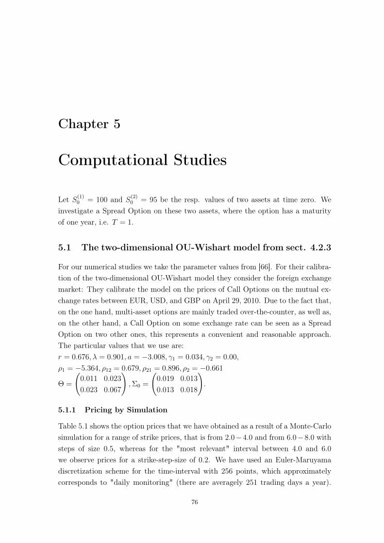
Chapter 5

Computational Studies

Let S(1)0 = 100 and S

(2)0 = 95 be the resp. values of two assets at time zero. We

investigate a Spread Option on these two assets, where the option has a maturityof one year, i.e. T = 1.

5.1 The two-dimensional OU-Wishart model from sect. 4.2.3

For our numerical studies we take the parameter values from [66]. For their calibra-tion of the two-dimensional OU-Wishart model they consider the foreign exchangemarket: They calibrate the model on the prices of Call Options on the mutual ex-change rates between EUR, USD, and GBP on April 29, 2010. Due to the fact that,on the one hand, multi-asset options are mainly traded over-the-counter, as well as,on the other hand, a Call Option on some exchange rate can be seen as a SpreadOption on two other ones, this represents a convenient and reasonable approach.The particular values that we use are:r = 0.676, λ = 0.901, a = −3.008, γ1 = 0.034, γ2 = 0.00,

ρ1 = −5.364, ρ12 = 0.679, ρ21 = 0.896, ρ2 = −0.661

Θ =

(0.011 0.023

0.023 0.067

),Σ0 =

(0.019 0.013

0.013 0.018

).

5.1.1 Pricing by Simulation

Table 5.1 shows the option prices that we have obtained as a result of a Monte-Carlosimulation for a range of strike prices, that is from 2.0−4.0 and from 6.0−8.0 withsteps of size 0.5, whereas for the "most relevant" interval between 4.0 and 6.0

we observe prices for a strike-step-size of 0.2. We have used an Euler-Maruyamadiscretization scheme for the time-interval with 256 points, which approximatelycorresponds to "daily monitoring" (there are averagely 251 trading days a year).

76

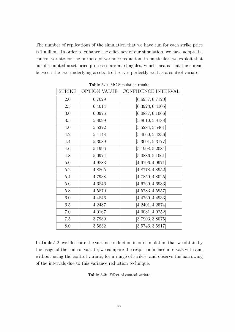
The number of replications of the simulation that we have run for each strike priceis 1 million. In order to enhance the efficiency of our simulation, we have adopted acontrol variate for the purpose of variance reduction; in particular, we exploit thatour discounted asset price processes are martingales, which means that the spreadbetween the two underlying assets itself serves perfectly well as a control variate.

Table 5.1: MC Simulation results

STRIKE OPTION VALUE CONFIDENCE INTERVAL

2.0 6.7029 [6.6937, 6.7120]

2.5 6.4014 [6.3923, 6.4105]

3.0 6.0976 [6.0887, 6.1066]

3.5 5.8099 [5.8010, 5.8188]

4.0 5.5372 [5.5284, 5.5461]

4.2 5.4148 [5.4060, 5.4236]

4.4 5.3089 [5.3001, 5.3177]

4.6 5.1996 [5.1908, 5.2084]

4.8 5.0974 [5.0886, 5.1061]

5.0 4.9883 [4.9796, 4.9971]

5.2 4.8865 [4.8778, 4.8952]

5.4 4.7938 [4.7850, 4.8025]

5.6 4.6846 [4.6760, 4.6933]

5.8 4.5870 [4.5783, 4.5957]

6.0 4.4846 [4.4760, 4.4933]

6.5 4.2487 [4.2401, 4.2574]

7.0 4.0167 [4.0081, 4.0252]

7.5 3.7989 [3.7903, 3.8075]

8.0 3.5832 [3.5746, 3.5917]

In Table 5.2, we illustrate the variance reduction in our simulation that we obtain bythe usage of the control variate; we compare the resp. confidence intervals with andwithout using the control variate, for a range of strikes, and observe the narrowingof the intervals due to this variance reduction technique.

Table 5.2: Effect of control variate

77

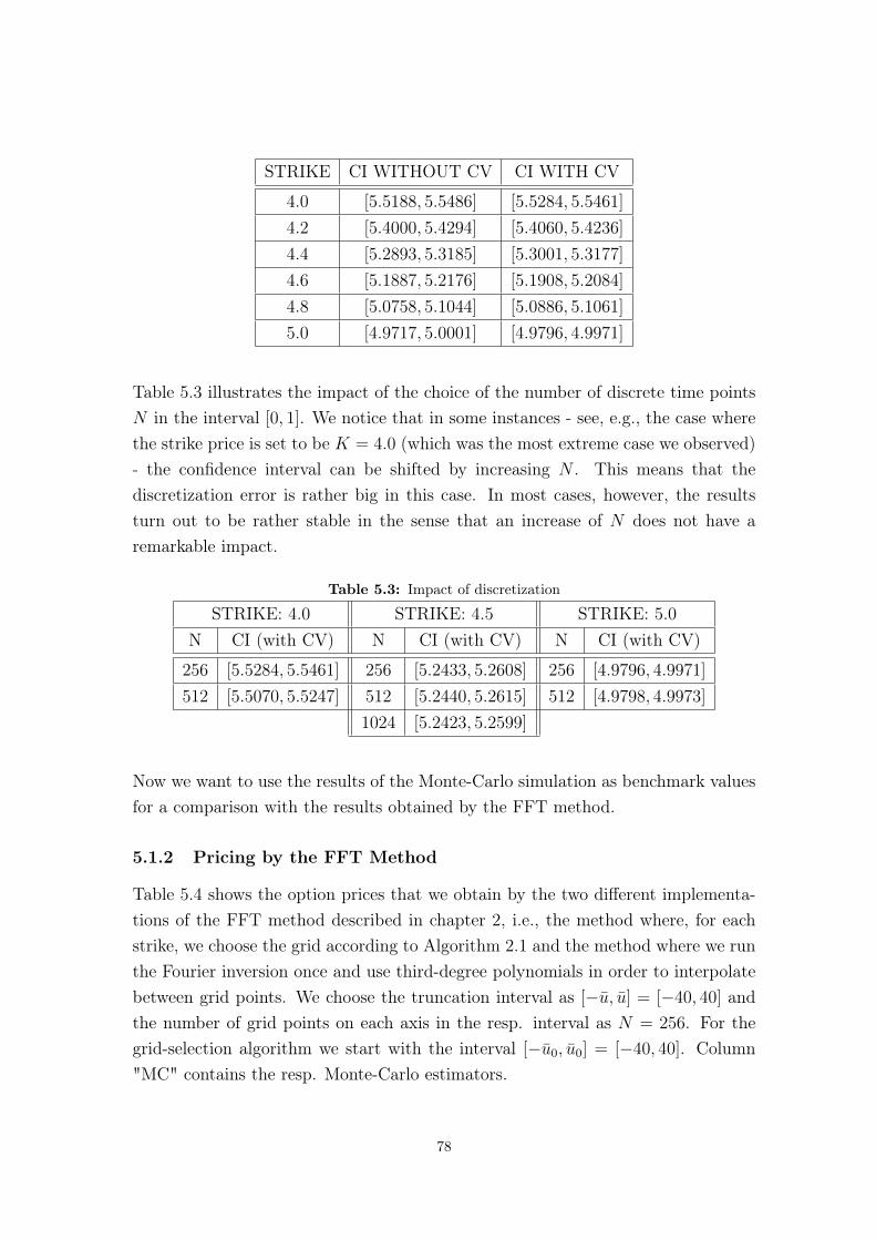
STRIKE CI WITHOUT CV CI WITH CV

4.0 [5.5188, 5.5486] [5.5284, 5.5461]

4.2 [5.4000, 5.4294] [5.4060, 5.4236]

4.4 [5.2893, 5.3185] [5.3001, 5.3177]

4.6 [5.1887, 5.2176] [5.1908, 5.2084]

4.8 [5.0758, 5.1044] [5.0886, 5.1061]

5.0 [4.9717, 5.0001] [4.9796, 4.9971]

Table 5.3 illustrates the impact of the choice of the number of discrete time pointsN in the interval [0, 1]. We notice that in some instances - see, e.g., the case wherethe strike price is set to be K = 4.0 (which was the most extreme case we observed)- the confidence interval can be shifted by increasing N . This means that thediscretization error is rather big in this case. In most cases, however, the resultsturn out to be rather stable in the sense that an increase of N does not have aremarkable impact.

Table 5.3: Impact of discretization

STRIKE: 4.0 STRIKE: 4.5 STRIKE: 5.0

N CI (with CV) N CI (with CV) N CI (with CV)

256 [5.5284, 5.5461] 256 [5.2433, 5.2608] 256 [4.9796, 4.9971]

512 [5.5070, 5.5247] 512 [5.2440, 5.2615] 512 [4.9798, 4.9973]

1024 [5.2423, 5.2599]

Now we want to use the results of the Monte-Carlo simulation as benchmark valuesfor a comparison with the results obtained by the FFT method.

5.1.2 Pricing by the FFT Method

Table 5.4 shows the option prices that we obtain by the two different implementa-tions of the FFT method described in chapter 2, i.e., the method where, for eachstrike, we choose the grid according to Algorithm 2.1 and the method where we runthe Fourier inversion once and use third-degree polynomials in order to interpolatebetween grid points. We choose the truncation interval as [−u, u] = [−40, 40] andthe number of grid points on each axis in the resp. interval as N = 256. For thegrid-selection algorithm we start with the interval [−u0, u0] = [−40, 40]. Column"MC" contains the resp. Monte-Carlo estimators.

78

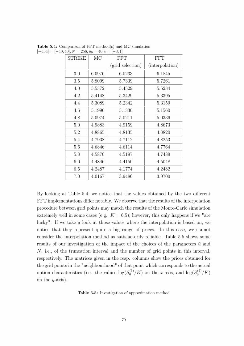
Table 5.4: Comparison of FFT method(s) and MC simulation[−u, u] = [−40, 40], N = 256, u0 = 40, ε = [−3, 1]

STRIKE MC FFT(grid selection)

FFT(interpolation)

3.0 6.0976 6.0233 6.1845

3.5 5.8099 5.7339 5.7261

4.0 5.5372 5.4529 5.5234

4.2 5.4148 5.3429 5.3395

4.4 5.3089 5.2342 5.3159

4.6 5.1996 5.1330 5.1560

4.8 5.0974 5.0211 5.0336

5.0 4.9883 4.9159 4.8673

5.2 4.8865 4.8135 4.8820

5.4 4.7938 4.7112 4.8253

5.6 4.6846 4.6114 4.7764

5.8 4.5870 4.5197 4.7489

6.0 4.4846 4.4150 4.5048

6.5 4.2487 4.1774 4.2482

7.0 4.0167 3.9486 3.9700

By looking at Table 5.4, we notice that the values obtained by the two differentFFT implementations differ notably. We observe that the results of the interpolationprocedure between grid points may match the results of the Monte-Carlo simulationextremely well in some cases (e.g., K = 6.5); however, this only happens if we "arelucky". If we take a look at those values where the interpolation is based on, wenotice that they represent quite a big range of prices. In this case, we cannotconsider the interpolation method as satisfactorily reliable. Table 5.5 shows someresults of our investigation of the impact of the choices of the parameters u andN , i.e., of the truncation interval and the number of grid points in this interval,respectively. The matrices given in the resp. columns show the prices obtained forthe grid points in the "neighbourhood" of that point which corresponds to the actualoption characteristics (i.e. the values log(S

(1)0 /K) on the x-axis, and log(S

(2)0 /K)

on the y-axis).

Table 5.5: Investigation of approximation method

79

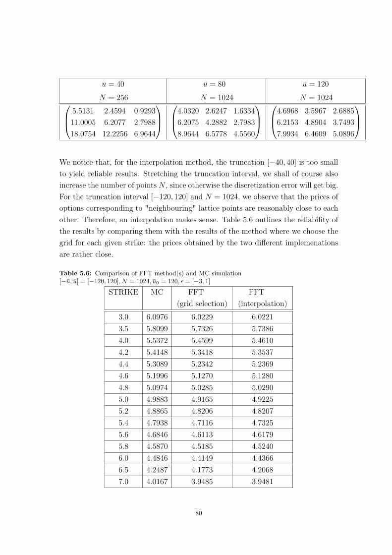
u = 40

N = 256

u = 80

N = 1024

u = 120

N = 1024 5.5131 2.4594 0.9293

11.0005 6.2077 2.7988

18.0754 12.2256 6.9644

4.0320 2.6247 1.6334

6.2075 4.2882 2.7983

8.9644 6.5778 4.5560

4.6968 3.5967 2.6885

6.2153 4.8904 3.7493

7.9934 6.4609 5.0896

We notice that, for the interpolation method, the truncation [−40, 40] is too smallto yield reliable results. Stretching the truncation interval, we shall of course alsoincrease the number of points N , since otherwise the discretization error will get big.For the truncation interval [−120, 120] and N = 1024, we observe that the prices ofoptions corresponding to "neighbouring" lattice points are reasonably close to eachother. Therefore, an interpolation makes sense. Table 5.6 outlines the reliability ofthe results by comparing them with the results of the method where we choose thegrid for each given strike: the prices obtained by the two different implemenationsare rather close.

Table 5.6: Comparison of FFT method(s) and MC simulation[−u, u] = [−120, 120], N = 1024, u0 = 120, ε = [−3, 1]

STRIKE MC FFT(grid selection)

FFT(interpolation)

3.0 6.0976 6.0229 6.0221

3.5 5.8099 5.7326 5.7386

4.0 5.5372 5.4599 5.4610

4.2 5.4148 5.3418 5.3537

4.4 5.3089 5.2342 5.2369

4.6 5.1996 5.1270 5.1280

4.8 5.0974 5.0285 5.0290

5.0 4.9883 4.9165 4.9225

5.2 4.8865 4.8206 4.8207

5.4 4.7938 4.7116 4.7325

5.6 4.6846 4.6113 4.6179

5.8 4.5870 4.5185 4.5240

6.0 4.4846 4.4149 4.4366

6.5 4.2487 4.1773 4.2068

7.0 4.0167 3.9485 3.9481

80

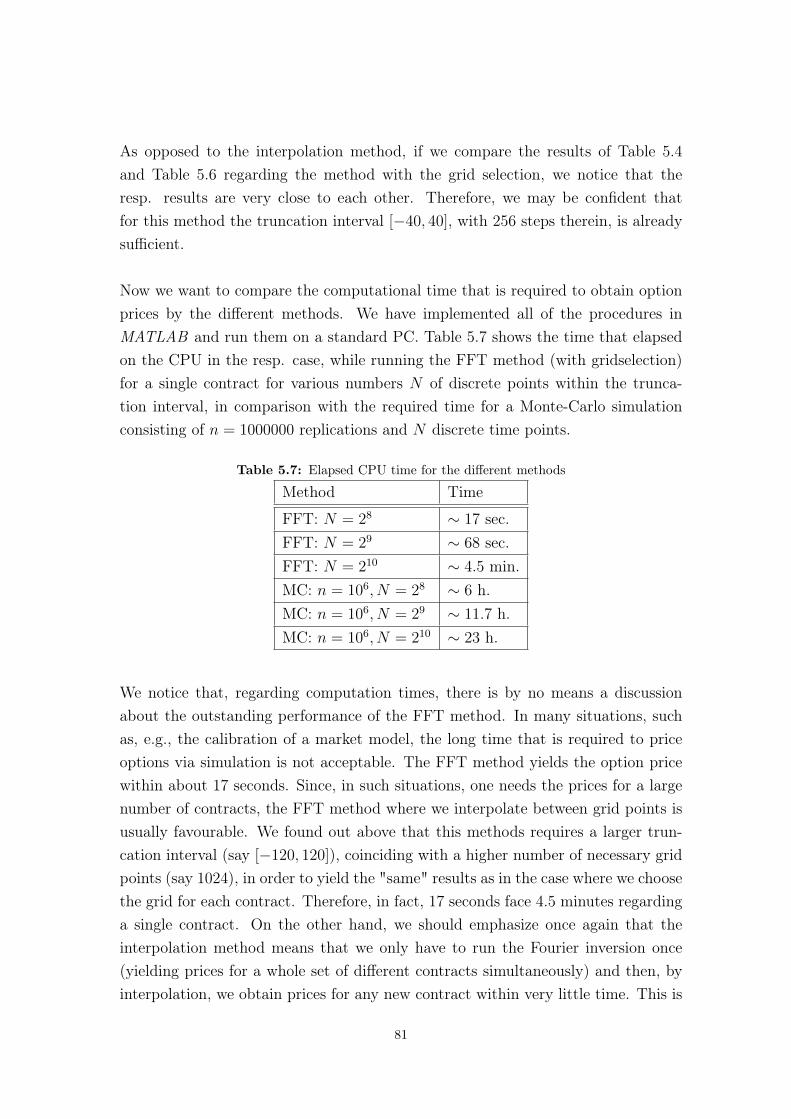
As opposed to the interpolation method, if we compare the results of Table 5.4and Table 5.6 regarding the method with the grid selection, we notice that theresp. results are very close to each other. Therefore, we may be confident thatfor this method the truncation interval [−40, 40], with 256 steps therein, is alreadysufficient.

Now we want to compare the computational time that is required to obtain optionprices by the different methods. We have implemented all of the procedures inMATLAB and run them on a standard PC. Table 5.7 shows the time that elapsedon the CPU in the resp. case, while running the FFT method (with gridselection)for a single contract for various numbers N of discrete points within the trunca-tion interval, in comparison with the required time for a Monte-Carlo simulationconsisting of n = 1000000 replications and N discrete time points.

Table 5.7: Elapsed CPU time for the different methods

Method Time

FFT: N = 28 ∼ 17 sec.FFT: N = 29 ∼ 68 sec.FFT: N = 210 ∼ 4.5 min.MC: n = 106, N = 28 ∼ 6 h.MC: n = 106, N = 29 ∼ 11.7 h.MC: n = 106, N = 210 ∼ 23 h.

We notice that, regarding computation times, there is by no means a discussionabout the outstanding performance of the FFT method. In many situations, suchas, e.g., the calibration of a market model, the long time that is required to priceoptions via simulation is not acceptable. The FFT method yields the option pricewithin about 17 seconds. Since, in such situations, one needs the prices for a largenumber of contracts, the FFT method where we interpolate between grid points isusually favourable. We found out above that this methods requires a larger trun-cation interval (say [−120, 120]), coinciding with a higher number of necessary gridpoints (say 1024), in order to yield the "same" results as in the case where we choosethe grid for each contract. Therefore, in fact, 17 seconds face 4.5 minutes regardinga single contract. On the other hand, we should emphasize once again that theinterpolation method means that we only have to run the Fourier inversion once(yielding prices for a whole set of different contracts simultaneously) and then, byinterpolation, we obtain prices for any new contract within very little time. This is

81

the reason why the FFT method with interpolation is usually unchallenged by othermethods, when it comes to simultaneously pricing many contracts. However, in ourcase, we have observed that we need to use many more discrete points N to obtainclose results with the interpolation method. Then, after we have run the Fourierinversion once (which takes for around 4.5 minutes, as mentioned above), the inter-polation (with a third degree polynomial) for every further contract yet (averagely)takes another 20 seconds. Therefore, we are still in favour of our method with thegrid selection, even regarding the pricing of a high number of contracts.

Our hitherto investigations within this chapter have shown the behaviour of theFFT method: we have illustrated for which parameter choices regarding truncationand discretization we may expect reliable results, and we have outlined the greatadvantage in terms of the computational speed. However, if we compare the result-ing option prices with those obtained by the Monte-Carlo method, the variation isnot negligible. It might be the case that, due to the jumps in the trajectories, somesimulation results change a bit if one uses higher numbers of discrete points. Wealready indicated this above, where we considered some examples (cf. Table 5.3).However, we have seen that with 1024 points, together with one million replications,it already takes almost one day to evaluate a single contract. Hence, it gets tediousto further increase the number of discretization points. In any case, regarding theFFT method, there is one parameter left that we have not investigated so far: thevector ε = [ε1, ε2], which is used to circumvent the issue with the integrability of thepayoff function.

On the choice of ε

We can see ε as the extension to two dimensions of what Carr and Madan [27]call the damping factor α, as described in section 2.1.2. In theory, this is only atechnical finesse. In practice, however, recall that the modified function is subjectto the numerical two-dimensional Fourier inversion. The only condition that wehave required was ε1 + ε2 < −1, where ε1, ε2 ∈ R with ε2 > 0. It seems evident thata reasonable choice of ε is neither obvious, nor is it a negligible issue. Particularlyin the two-dimensional case, the choice of ε is, in fact, a crucial part of the pricingmodel. Table 5.8 shows some selected examples, outlining the strong impact of thisparameter.

Table 5.8: Investigation of the sensitivity of the model to changes in ε.Method with grid selection; u = [−40, 40], N = 256,K = 5

82

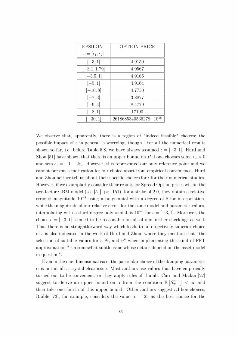
EPSILONε = [ε1, ε2]

OPTION PRICE

[−3, 1] 4.9159

[−3.1, 1.79] 4.9567

[−3.5, 1] 4.9166

[−5, 1] 4.9164

[−10, 8] 4.7750

[−7, 3] 3.8877

[−9, 4] 8.4779

[−8, 1] 17190

[−30, 1] 2618685340536278 · 1018

We observe that, apparently, there is a region of "indeed feasible" choices; thepossible impact of ε in general is worrying, though. For all the numerical resultsshown so far, i.e. before Table 5.8, we have always assumed ε = [−3, 1]. Hurd andZhou [51] have shown that there is an upper bound on P if one chooses some ε2 > 0

and sets ε1 = −1− 2ε2. However, this represented our only reference point and wecannot present a motivation for our choice apart from empirical convenience. Hurdand Zhou neither tell us about their specific choices for ε for their numerical studies.However, if we examplarily consider their results for Spread Option prices within thetwo-factor GBM model (see [51], pg. 151), for a strike of 2.0, they obtain a relativeerror of magnitude 10−8 using a polynomial with a degree of 8 for interpolation,while the magnitude of our relative error, for the same model and parameter values,interpolating with a third-degree polynomial, is 10−4 for ε = [−3, 1]. Moreover, thechoice ε = [−3, 1] seemed to be reasonable for all of our further checkings as well.That there is no straightforward way which leads to an objectively superior choiceof ε is also indicated in the work of Hurd and Zhou, where they mention that "theselection of suitable values for ε,N , and η" when implementing this kind of FFTapproximation "is a somewhat subtle issue whose details depend on the asset modelin question".

Even in the one-dimensional case, the particular choice of the damping parameterα is not at all a crystal-clear issue. Most authors use values that have empiricallyturned out to be convenient, or they apply rules of thumb: Carr and Madan [27]suggest to derive an upper bound on α from the condition E

[Sα+1T

]< ∞ and

then take one fourth of this upper bound. Other authors suggest ad-hoc choices;Raible [73], for example, considers the value α = 25 as the best choice for the

83

models he studies. A rigorous investigation of the issue of an appropriate choiceof α has been presented by Lord and Kahl [60]: they address the problem that, asthey formulate it in particular, "by changing α, the integrand can become eitherstrongly peaked when getting close to the poles of the integrand, or highly oscillatorywhen reaching the maximum allowed α", by formulating an optimality criterionand solving the resulting optimization problem. In particular, they both suggestan optimal choice of α depending on the payoff as well as a payoff-independentalternative of choosing the damping parameter.

In the case of Spread Options, i.e., in the case of two dimensions, the methodof Lord and Kahl cannot be applied directly. We face a two-dimensional vector εinstead of the one-dimensional α, which renders it more complicated to formulatean appropriate optimization problem. For a satisfactory degree of reliability of thepricing method it would be necessary, though, to pose some optimality criterion onε. This would be a way to detach the model from any empirically motivated ad-hocdecisions and add confidence about the results. However, we do not consider thisas a scope of this thesis and hence do not try to follow this path here.

Since, as described above, the impact of the choice of ε does not indeed allowholistic satisfaction with the method, we now want to check alternative approachesfor applicability in the context of Spread Options, with the intention to possiblyavoid the concept of multiplying the payoff in order to ensure integrability.

The method with time-values

In section 2.1.2 we described the idea of Carr and Madan [27] to use the time-valueof an option, i.e., to subtract the intrinsic value from the option price, in order toavoid the damping factor but ensure integrability of the modified option price asa function in strike. However, this idea is unfortunately not extendable to SpreadOptions: What Hurd and Zhou have suggested as an extension of the Carr andMadan method to the case of Spread Options, as we described in detail in section2.1.3, is that they have found a representation of the modified (multiplied by afactor which ensures integrability) payoff function (not option price as function instrike) by Fourier inversion; the (discounted) expected value then corresponds to arepresentation of the option price which contains the joint characteristic functionof the underlying assets.

The idea with subtracting the intrinsic value only makes sense if one considers theoption price as a function in strike and wants to circumvent the problem that thisoption pricing function is not (square-)integrable. This works perfectly well in the

84

one-dimensional case: they’ve worked out the details for a Call Option, where theyobtain a closed-form expression for the Fourier transform of the option’s time-value,which contains the characteristic function of the underlying asset. Consequently,Fourier inversion yields the desired representation.

However, considering Spread Options, the problem with this strategy is thatthe strike is still (as for a vanilla option) one-dimensional, whereas now one facestwo asset-price processes and the density depends on both assets. Following ananalogous strategy as for a Call Option, i.e., to start with the option’s time-value asa function in strike and proceed with rearranging its Fourier transform, hence doesnot render it possible to obtain a closed-form expression of the Fourier transform ofthe time-value, which contains the joint characteristic function of the two underlyingassets.

The Integration-Along-Cut method

As we have seen, the FFT method has its drawbacks; particularly, we are not gladabout the fact that there is no general effective procedure available in order to choosethe damping parameter (which can also be seen as choosing the line of integration).A different approach, which does not make use of the FFT and where there is noneed for a damping parameter, has been suggested in the book of Boyarchenko andLevendorskiı [23]. Their method, which they call the Integration-Along-Cut (IAC)method, allows for an effective control of the computational error and, moreover, inmany cases they even observe advantages with respect to the FFT method in termsof the computational speed when pricing single options. We therefore want to takea closer look at the IAC method and check its applicability for our purposes. Wedo not want to go into full detail in terms of technicalities but rather comment onthe crucial aspects. For details see [23].

The method is presented for a market model where the log-asset price is assumedto follow a CGMY(c,−λ−, λ+, ν) (the authors prefer the less common term KoBoLin their original work, which is an acronym for Koponen, Boyarchenko, Levendorskiı)process of order ν ∈ (0, 1). The skewness parameters are assumed to satisfy λ− <−1 < 0 < λ+. Consider a European Put Option with strike price K = 1, maturityT , and spot price of the asset given by S0 = ex. The Fourier transform of the payoff

85

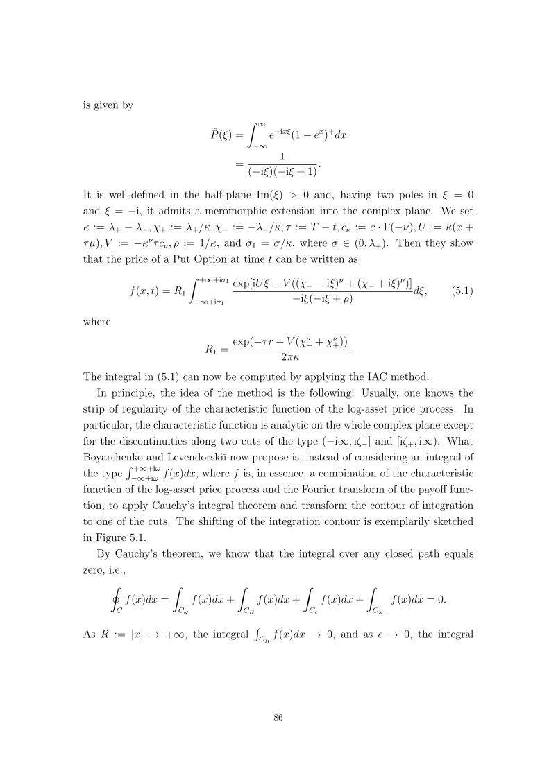
is given by

P (ξ) =

∫ ∞−∞

e−ixξ(1− ex)+dx

=1

(−iξ)(−iξ + 1).

It is well-defined in the half-plane Im(ξ) > 0 and, having two poles in ξ = 0

and ξ = −i, it admits a meromorphic extension into the complex plane. We setκ := λ+ − λ−, χ+ := λ+/κ, χ− := −λ−/κ, τ := T − t, cν := c · Γ(−ν), U := κ(x +

τµ), V := −κντcν , ρ := 1/κ, and σ1 = σ/κ, where σ ∈ (0, λ+). Then they showthat the price of a Put Option at time t can be written as

f(x, t) = R1

∫ +∞+iσ1

−∞+iσ1

exp[iUξ − V ((χ− − iξ)ν + (χ+ + iξ)ν)]

−iξ(−iξ + ρ)dξ, (5.1)

where

R1 =exp(−τr + V (χν− + χν+))

2πκ.

The integral in (5.1) can now be computed by applying the IAC method.In principle, the idea of the method is the following: Usually, one knows the

strip of regularity of the characteristic function of the log-asset price process. Inparticular, the characteristic function is analytic on the whole complex plane exceptfor the discontinuities along two cuts of the type (−i∞, iζ−] and [iζ+, i∞). WhatBoyarchenko and Levendorskiı now propose is, instead of considering an integral ofthe type

∫ +∞+iω

−∞+iωf(x)dx, where f is, in essence, a combination of the characteristic

function of the log-asset price process and the Fourier transform of the payoff func-tion, to apply Cauchy’s integral theorem and transform the contour of integrationto one of the cuts. The shifting of the integration contour is exemplarily sketchedin Figure 5.1.

By Cauchy’s theorem, we know that the integral over any closed path equalszero, i.e.,∮

C

f(x)dx =

∫Cω

f(x)dx+

∫CR

f(x)dx+

∫Cε

f(x)dx+

∫Cλ−

f(x)dx = 0.

As R := |x| → +∞, the integral∫CRf(x)dx → 0, and as ε → 0, the integral

86

Figure 5.1: Contour shift

CR

Cε

Cω

Cλ−

[iλ−,−i∞)

λ

ω

∫Cεf(x)dx→ 0. Therefore, we can write∫

Im(x)=ω

f(x)dx =

∫ iλ−−0

−i∞−0

f(x)dx+

∫ −i∞+0

iλ−+0

f(x)dx.

Let us now get back to the particular case of the CGMY process, where we "stopped"at (5.1):

In the case U ≥ 0, the contour of integration is shifted to the cut in the upperhalf-plane (the cuts result from the strip of analyticity of the characteristic functionof a CGMY process). The choice of the cut is due to the intention that iUξ benegative at the cut, i.e., exp(iUξ) shall not grow to infinity. By setting aν :=

cos(νπ), bν := sin(νπ) and performing some rearranging steps, including variablesubstitutions, the option price can be written as

f(x, t) = 2R1e−Uχ+I(ν, U, V, χ+, χ+ + ρ), (5.2)

where

I(ν, u, v, ρ1, ρ2) :=

∫ ∞0

e−zu sin(vbνzν)

(z + ρ1)(z + ρ2)exp(−v[(1 + z)ν + aνz

ν ])dz. (5.3)

The integral (5.3) can be evaluated using any numerical integration prodecure,yielding the option price as a result of (5.2), for the case U ≥ 0.

87

In the case U < 0, the contour of integration is shifted to the cut in the lowerhalf-plane. This transformation means that one has to take into account the twopoles ξ = 0 and ξ = −i. The residue theorem can then be used to express theintegral in terms of the new contour, and by rearranging and changing variablesone can obtain the representation

f(x, t) = exp(−τr)− exp(x) + 2R1eUχ−I(ν,−U, V, χ−, χ− − ρ),

with the function I as defined in (5.3).

Now we have seen how the IAC technique works and that it is very well suited for thepricing of vanilla options in the CGMY model. It is also applicable in many othersituations, and the performance of the method is particularly good if the option isclose to maturity. However, the method is not generally applicable to any model;for example, Lord and Kahl [60] mention some cases where problems arise. Letus now take a look at our situation of Spread Options in the two-dimensional OUtype SV model (where the OU Wishart model is a special case thereof). Theorem4.6 gives information about the regularity of the moment-generating function in themulti-dimensional OU type SV model. The strip of analyticity of the characteristicfunction is consequently given by

Sφθ := y ∈ Cd : ‖ Im(y)‖ < θ,

with θ as defined in the theorem. As a consequence of Theorem 2.1, equation (2.11)gives the price of a Spread Option as

Spr(X0;T ) =1

(2π)2e−rT

∫ ∫R2+iε

eiuXt0φXT (u)P (u)d2u,

where

P (u) =Γ(i(u1 + u2)− 1)Γ(−iu2)

Γ(iu1 + 1).

The Gamma function has poles of first order in all non-positive integers. Therefore,shifting the contour of integration to the cuts means that we cross infinitely manypoles. A straightforward application of the residue theorem is thus not possible andthe IAC method is in further consequence not easily applicable.

There are generalizations of the residue theorem, which deal with infinite num-bers of isolated singularities; roughly speaking, the real axis is "closed at infinity" bya semi-circle. Carefulness is required in this case, though, and some more work will

88

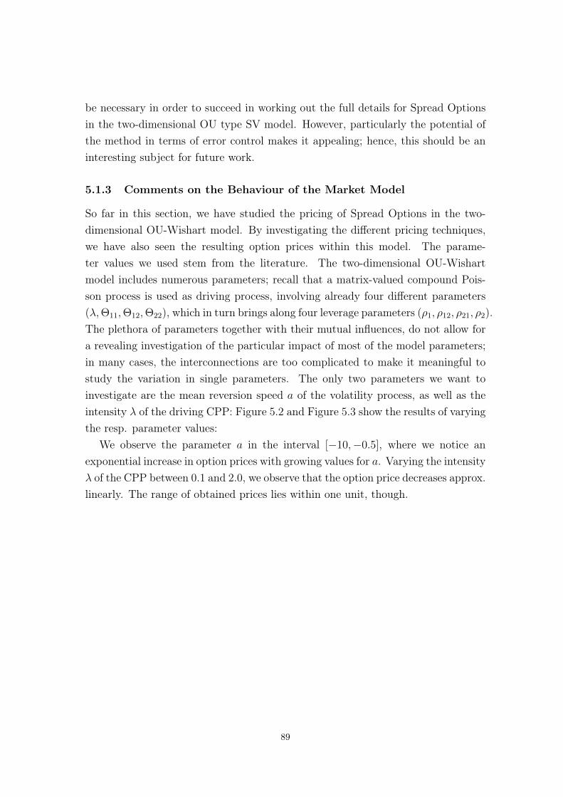
be necessary in order to succeed in working out the full details for Spread Optionsin the two-dimensional OU type SV model. However, particularly the potential ofthe method in terms of error control makes it appealing; hence, this should be aninteresting subject for future work.

5.1.3 Comments on the Behaviour of the Market Model

So far in this section, we have studied the pricing of Spread Options in the two-dimensional OU-Wishart model. By investigating the different pricing techniques,we have also seen the resulting option prices within this model. The parame-ter values we used stem from the literature. The two-dimensional OU-Wishartmodel includes numerous parameters; recall that a matrix-valued compound Pois-son process is used as driving process, involving already four different parameters(λ,Θ11,Θ12,Θ22), which in turn brings along four leverage parameters (ρ1, ρ12, ρ21, ρ2).The plethora of parameters together with their mutual influences, do not allow fora revealing investigation of the particular impact of most of the model parameters;in many cases, the interconnections are too complicated to make it meaningful tostudy the variation in single parameters. The only two parameters we want toinvestigate are the mean reversion speed a of the volatility process, as well as theintensity λ of the driving CPP: Figure 5.2 and Figure 5.3 show the results of varyingthe resp. parameter values:

We observe the parameter a in the interval [−10,−0.5], where we notice anexponential increase in option prices with growing values for a. Varying the intensityλ of the CPP between 0.1 and 2.0, we observe that the option price decreases approx.linearly. The range of obtained prices lies within one unit, though.

89

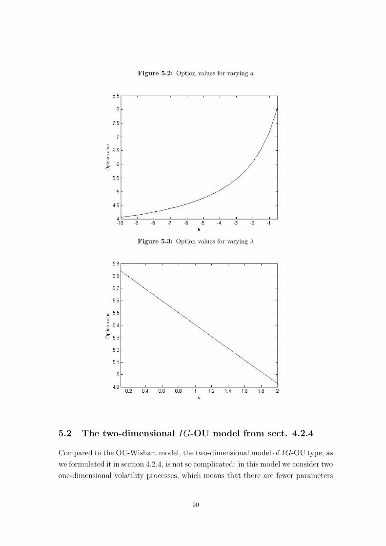
Figure 5.2: Option values for varying a

Figure 5.3: Option values for varying λ

5.2 The two-dimensional IG-OU model from sect. 4.2.4

Compared to the OU-Wishart model, the two-dimensional model of IG-OU type, aswe formulated it in section 4.2.4, is not so complicated: in this model we consider twoone-dimensional volatility processes, which means that there are fewer parameters

90

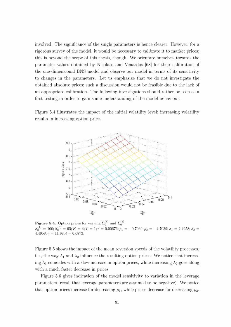
involved. The significance of the single parameters is hence clearer. However, for arigorous survey of the model, it would be necessary to calibrate it to market prices;this is beyond the scope of this thesis, though. We orientate ourselves towards theparameter values obtained by Nicolato and Venardos [68] for their calibration ofthe one-dimensional BNS model and observe our model in terms of its sensitivityto changes in the parameters. Let us emphasize that we do not investigate theobtained absolute prices; such a discussion would not be feasible due to the lack ofan appropriate calibration. The following investigations should rather be seen as afirst testing in order to gain some understanding of the model behaviour.

Figure 5.4 illustrates the impact of the initial volatility level; increasing volatilityresults in increasing option prices.

Figure 5.4: Option prices for varying Σ(1)0 and Σ

(2)0 .

S(1)0 = 100;S

(2)0 = 95;K = 4;T = 1; r = 0.00676; ρ1 = −0.7039; ρ2 = −4.7039;λ1 = 2.4958;λ2 =

4.4958; γ = 11.98; δ = 0.0872;

Figure 5.5 shows the impact of the mean reversion speeds of the volatility processes,i.e., the way λ1 and λ2 influence the resulting option prices. We notice that increas-ing λ1 coincides with a slow increase in option prices, while increasing λ2 goes alongwith a much faster decrease in prices.

Figure 5.6 gives indication of the model sensitivity to variation in the leverageparameters (recall that leverage parameters are assumed to be negative). We noticethat option prices increase for decreasing ρ1, while prices decrease for decreasing ρ2.

91

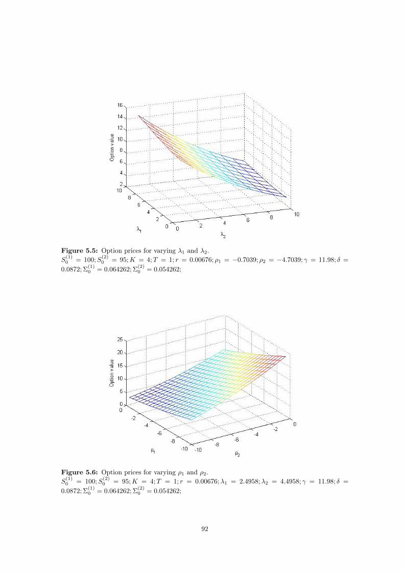
Figure 5.5: Option prices for varying λ1 and λ2.S(1)0 = 100;S

(2)0 = 95;K = 4;T = 1; r = 0.00676; ρ1 = −0.7039; ρ2 = −4.7039; γ = 11.98; δ =

0.0872; Σ(1)0 = 0.064262; Σ

(2)0 = 0.054262;

Figure 5.6: Option prices for varying ρ1 and ρ2.S(1)0 = 100;S

(2)0 = 95;K = 4;T = 1; r = 0.00676;λ1 = 2.4958;λ2 = 4.4958; γ = 11.98; δ =

0.0872; Σ(1)0 = 0.064262; Σ

(2)0 = 0.054262;

92

Chapter 6

Conclusion

In this thesis, we have discussed the pricing of Spread Options in multivariateOrnstein-Uhlenbeck type stochastic volatility models, which are driven by matrixsubordinators. On the one hand, this included an investigation of different pricingtechniques: we ran Monte-Carlo simulations and we compared the results with thoseobtained by an FFT method, which had been developed by Hurd and Zhou [51].On the other hand, we examined different specifications of the market model, bothfrom a qualitative and a quantitative point of view.

Regarding the pricing techniques, we analyzed the FFT method in detail, whichrevealed its advantages and weaknesses. We compared two possible ways of deal-ing with the issue of applying the method to any given set of spot prices of theunderlying assets and strike price; we presented an algorithm to choose the latticefor approximation in an appropriate way for any particular contract on the onehand, and we implemented an interpolation procedure on the other hand. Thecomputational speed of the FFT method is outstanding. The short computationtime required to calculate option prices makes it appealing, particularly in caseswhere many contracts are involved. The main shortcoming of the method, whichgives us some cause for concern, is the sensitivity to that parameter vector, whichis used to modify the payoff function in order to ensure integrability and, in furtherconsequence, existence of its Fourier transform. We observed that the impact ofthe particular choice of this parameter vector can be very strong; a sensible choiceis hence an absolute necessity. However, there are no routines available to find anobjectively superior choice. One has to make an ad-hoc decision, solely based onempirical convenience. We consider this as a clear drawback of this method. There-fore, we also studied alternative approaches for applicability; particularly, the IACmethod appears to have potential, which represents an interesting starting point forfuture work.

93

In terms of the multivariate Ornstein-Uhlenbeck type stochastic volatility model,we first surveyed the literature about this model. We started with the one-dimensionalBNS model (Barndorff-Nielsen and Shephard [6,7]) and discussed the necessary the-ory in order to be able to finally formulate the multivariate extension along the linesof Muhle-Karbe, Pfaffel, and Stelzer [66]. We took a particular specification of thismodel (which has also been presented in their work), namely, the two-dimensionalOU-Wishart model and computed explicit prices for Spread Options. From a mod-elling point of view, we particularly addressed the issue of prespecifying the invariantdistribution of the volatility process in the multi-dimensional case. Considering theinverse Gaussian distribution on a positive semidefinite cone, this is still an openissue in the very general case. However, under some simplifying assumptions, weformulated a model as a special case: we took two one-dimensional volatility pro-cesses with stationary distribution of the inverse Gaussian type, both driven byone and the same BDLP. We derived the joint characteristic function of the (two-dimensional) log-return process and finally also examined a first testing of parametersensitivities. Moreover, as a part of our modelling attempts, we noticed that usingtwo correlated Brownian motions would break the affine structure of the model.

In the course of the development of this thesis, various questions have arisen. Asalready mentioned above, the details of the correspondence between the BDLP andthe stationary distribution of an Ornstein-Uhlenbeck process need to be extendedto the multi-dimensional case: It would be an interesting advancement to be able toprespecify a (matrix-valued) IG-law for the volatility process and work out the fulldetails for the BDLP, making it possible to simulate from it. On the other hand,succeeding in deriving the joint characteristic function of the log-return process inthis model would enable us to apply transform-based option pricing methods.

As a further step, a calibration to market prices of the multivariate IG-OU modelwill be necessary. For the special case that we considered, given an appropriate dataset, we would already have the tools to do so by applying the FFT method and usingthe characteristic function, which we successfully derived. It would be especiallyinteresting to calibrate the model on energy derivatives, since in the modelling ofenergy markets, stochastic volatility models with jumps have attracted particularattention.

Finally, enhancement of the computational methods will be necessary in orderto deal with the numerical issues raised above. From a mathematical point of view,further development of the rather elegant IAC method seems particularly attractive.

94

References

[1] M. Abramowitz and I. A. Stegun. Handbook of Mathematical Functions withFormulas, Graphs, and Mathematical Tables. Dover, New York, ninth Doverprinting, tenth GPO printing edition, 1964.

[2] H. Albrecher and M. Predota. On Asian Option Pricing for NIG Lévy Processes.J. Comput. Appl. Math., 172(1):153–168, November 2004.

[3] D. Applebaum. Lévy Processes and Stochastic Calculus. Cambridge UniversityPress, 2004.

[4] O. E. Barndorff-Nielsen. Normal inverse Gaussian distributions and stochasticvolatility modelling. Scand. J. Stat., 24(1):1–13, 1997.

[5] O. E. Barndorff-Nielsen. Processes of normal inverse Gaussian type. Financeand Stochastics, 2(1):41–68, 1997.

[6] O. E. Barndorff-Nielsen and N. Shephard. Modelling by Lévy Processes for Fi-nancial Econometrics. Economics Series Working Papers 2000-W03, Universityof Oxford, Department of Economics, January 2000.

[7] O. E. Barndorff-Nielsen and N. Shephard. Non-Gaussian Ornstein-Uhlenbeck-based models and some of their uses in financial economics. Journal of theRoyal Statistical Society Series B, 63(2):167–241, 2001.

[8] O. E. Barndorff-Nielsen and R. Stelzer. Positive-Definite Matrix Processes ofFinite Variation. Probability and Mathematical Statistics, 27(1):3–43, 2007.

[9] O.E. Barndorff-Nielsen. Superposition of Ornstein–Uhlenbeck type processes.Theory of Probability and its Applications, 45:175–194, 2001.

[10] O.E. Barndorff-Nielsen and V. Pérez-Abreu. Matrix subordinators and relatedupsilon transformations. Theory of Probability and its Applications, 52(1):1–23,2008.

95

[11] O.E. Barndorff-Nielsen and R. Stelzer. Multivariate supOU processes. Annalsof Applied Probability, 21:140–182, 2010.

[12] O.E. Barndorff-Nielsen and R. Stelzer. The multivariate supOU stochasticvolatility model. Mathematical Finance, 23(2):275–296, 2013.

[13] D. S. Bates. Jumps and Stochastic Volatility: Exchange Rate Processes Im-plicit in Deutsche Mark Options. Review of Financial Studies, 9(1):69–107,1996.

[14] F. E. Benth. The Stochastic Volatility Model of Barndorff-Nielsen and Shep-hard in Commodity Markets. Mathematical Finance, 21(4):595–625, 2011.

[15] F. E. Benth and L. Vos. Cross-commodity spot price modeling with stochasticvolatility and leverage for energy markets. Advances in Applied Probability,45(2):545–571, 06 2013.

[16] F. E. Benth and L. Vos. Pricing of forwards and options in a multivariate non-Gaussian stochastic volatility model for energy markets. Advances in AppliedProbability, 45(2):572–594, 06 2013.

[17] E. Bernadac. Random continued fractions and inverse Gaussian distributionon a symmetric cone. Journal of Theoretical Probability, 8(2):221–259, 1995.

[18] J. Bertoin. Lévy Processes. Cambridge Tracts in Mathematics. CambridgeUniversity Press, 1998.

[19] P. Bjerksund and G. Stensland. Closed form spread option valuation. Quanti-tative Finance, iFirst:1–10, 2011.

[20] F. Black and M. Scholes. The pricing of options and corporate liabilities.Journal of political economy, 81(3):637, 1973.

[21] S. Borovkova, F. Permana, and H. van der Weide. A Closed Form Approachto the Valuation and Hedging of Basket and Spread Options. The journal ofderivatives : the official publication of the International Association of Finan-cial Engineers, 14(4):8–24, 2007.

[22] J.-P. Bouchaud, A. Matacz, and M. Potters. The leverage effect in financialmarkets: retarded volatility and market panic. Science & Finance (CFM)working paper archive 0101120, Science & Finance, Capital Fund Management,2001.

96

[23] S.I. Boyarchenko and S.Z. Levendorskiı. Non-Gaussian Merton-Black-ScholesTheory. Advanced Series on Statistical Science and Applied Probability. WorldScientific Publishing Company, Incorporated, 2002.

[24] R. Caldana and G. Fusai. A general closed-form spread option pricing formula.Journal of Banking & Finance, 37(12):4893–4906, 2013.

[25] R. Carmona and V. Durrleman. Pricing and Hedging Spread Options. SIAMReview, 45:627–685, 2003.

[26] R. Carmona and V. Durrleman. Pricing and Hedging Spread Options in aLog-Normal Model. Working paper, Princeton Univ., 2003.

[27] P. P. Carr and D. B. Madan. Option Valuation Using the Fast Fourier Trans-form. Journal of Computational Finance, 2:61–73, 1999.

[28] R. Chhikara and J. Leroy Folks. The Inverse Gaussian Distribution: Theory:Methodology, and Applications. Statistics: A Series of Textbooks and Mono-graphs. Taylor & Francis, 1988.

[29] CME Group. Introduction to Crack Spreads. cmegroup.com, 2013.

[30] R. Cont. Empirical properties of asset returns: stylized facts and statisticalissues. Quantitative Finance, 1:223–236, 2001.

[31] R. Cont and P. Tankov. Financial modelling with jump processes. Chapman &Hall/CRC financial mathematics series. Chapman & Hall/CRC, Boca Raton,Fla., London, New York, 2004.

[32] J. Cooley and J. Tukey. An Algorithm for the Machine Calculation of ComplexFourier Series. Mathematics of Computation, 19(90):297–301, 1965.

[33] J. Cox, J. Ingersoll, and St. Ross. A Theory of the Term Structure of InterestRates. Econometrica, 53(2):385–407, March 1985.

[34] Ch. Cuchiero, D. Filipović, E. Mayerhofer, and J. Teichmann. Affine processeson positive semidefinite matrices. The Annals of Applied Probability, 21(2):397–463, 04 2011.

[35] Ch. Cuchiero, D. Filipović, and J. Teichmann. Affine Models. In Encyclopediaof Quantitative Finance. John Wiley & Sons, Ltd, 2010.

[36] M.A.H. Dempster and S.S.G. Hong. Spread Option Valuation and the FastFourier Transform. In H. Geman, D. Madan, St. R. Pliska, and T. Vorst,

97

editors, Mathematical Finance – Bachelier Congress 2000, Springer Finance,pages 203–220. Springer Berlin Heidelberg, 2002.

[37] S.J. Deng. Stochastic Models of Energy Commodity Prices and Their Appli-cations: Mean-reversion with Jumps and Spikes, 2000.

[38] S.J. Deng, M. Li, and J. Zhou. Multi-asset spread option pricing and hedging.Quant. Finance, 10(3):305–324, 2010.

[39] S.J. Deng and S.S. Oren. Electricity derivatives and risk management. Energy,31(6):940 – 953, 2006. Electricity Market Reform and Deregulation.

[40] D. Duffie, D. Filipović, and W. Schachermayer. Affine processes and applica-tions in finance. Annals of Applied Probability, 13:984–1053, 2003.

[41] J. B. C. Garcia, H. van Ginderen, and R. C. Garcia. On the Pricing of CreditSpread Options: A Two Factor HW-BK Algorithm. International Journal ofTheoretical and Applied Finance, 06(05):491–505, 2003.

[42] F. Gordon and S. Gordon. Characterizations of the Wishart distribution us-ing regression properties. Annals of the Institute of Statistical Mathematics,28(1):201–220, 1976.

[43] M. Groth. Topics in Computational Finance: The Barndorff-Nielsen & Shep-hard Stochastic Volatility Model. PhD thesis, University of Oslo, 2007.

[44] M. T. Heideman, D. H. Johnson, and C. S. Burrus. Gauss and the history of thefast Fourier transform. Archive for History of Exact Sciences, 34(3):265–277,1985.

[45] S. L. Heston. A Closed-Form Solution for Options with Stochastic Volatilitywith Applications to Bond and Currency Options. Review of Financial Studies,6:327–343, 1993.

[46] F. Hubalek and E. Nicolato. On multivariate extensions of Lévy drivenOrnstein-Uhlenbeck type stochastic volatility models and multi-asset options.Preprint, 2005.

[47] F. Hubalek and C. Sgarra. On the Esscher transforms and other equivalentmartingale measures for Barndorff-Nielsen and Shephard stochastic volatilitymodels with jumps. Stochastic Processes and their Applications, 119(7):2137 –2157, 2009.

98

[48] F. Hubalek and C. Sgarra. On the explicit evaluation of the Geometric Asianoptions in stochastic volatility models with jumps. J. Computational AppliedMathematics, 235(11):3355–3365, 2011.

[49] J. C. Hull. Options, Futures, and Other Derivatives. Pearson Prentice Hall,Upper Saddle River, NJ [u.a.], 6. ed., pearson internat. ed edition, 2006.

[50] J. C. Hull and A. D. White. The Pricing of Options on Assets with StochasticVolatilities. Journal of Finance, 42(2):281–300, June 1987.

[51] T. R. Hurd and Z. Zhou. A Fourier Transform Method for Spread OptionPricing. SIAM J. Financial Math., 1(1):142–157, 2010.

[52] J. Jacod and A.N. Shiryaev. Limit Theorems for Stochastic Processes.Grundlehren der mathematischen Wissenschaften. Springer-Verlag, 1987.

[53] Z. J. Jurek. Remarks on the selfdecomposability and new examples. Demon-stratio Mathematica, XXXIV:241–250, 2001.

[54] Z. J. Jurek and W. Vervaat. An integral representation for selfdecomposableBanach space valued random variables. Zeitschrift für Wahrscheinlichkeitsthe-orie und Verwandte Gebiete, 62(2):247–262, 1983.

[55] Z.J. Jurek and J.D. Mason. Operator-limit Distributions in Probability The-ory. Wiley series in probability and mathematical statistics: Probability andmathematical statistics. Wiley, 1993.

[56] M. Keller-Ressel. Affine processes - theory and applications in finance. Phdthesis, Vienna University of Technology, 2008.

[57] E. Kirk. Correlation in the Energy Markets. In V. Kaminski, editor, In:Managing Energy Price Risk, pages 71–78. London: Risk Publication, firstedition, 1995.

[58] S. G. Kou. A Jump-Diffusion Model for Option Pricing. Manage. Sci.,48(8):1086–1101, August 2002.

[59] J. Lillestøl. Risk analysis and the NIG distribution. Journal of Risk, 2000.

[60] R. Lord and Ch. Kahl. Optimal Fourier inversion in semi-analytical optionpricing. Tinbergen Institute Discussion Papers 06-066/2, Tinbergen Institute,2006.

[61] B. Mandelbrot. The Variation of Certain Speculative Prices. The Journal ofBusiness, 36:394, 1963.

99

[62] M. B. Marcus. Xé -radial Processes and Random Fourier Series. Number 368in Memoirs Series. American Mathematical Society, 1987.

[63] W. Margrabe. The Value of an Option to Exchange One Asset for Another.Journal of Finance, 33(1):177–86, March 1978.

[64] R. C. Merton. Theory of Rational Option Pricing. Bell Journal of Economics,4(1):141–183, Spring 1973.

[65] R. C. Merton. Option pricing when underlying stock returns are discontinuous.Journal of Financial Economics, 3:125–144, 1976.

[66] J. Muhle-Karbe, O. Pfaffel, and R. Stelzer. Option Pricing in MultivariateStochastic Volatility Models of OU Type. SIAM J. Financial Math., 3(1):66–94, 2012.

[67] D. B. Nelson. Conditional Heteroskedasticity in Asset Returns: A New Ap-proach. Econometrica, 59(2):347–370, March 1991.

[68] E. Nicolato and E. Venardos. Option Pricing in Stochastic Volatility Modelsof the Ornstein-Uhlenbeck Type. Mathematical Finance, 13(4):445–466, 2003.

[69] N. D. Pearson. An Efficient Approach for Pricing Spread Options. The jour-nal of derivatives : the official publication of the International Association ofFinancial Engineers., 1995.

[70] Ch. Pigorsch and R. Stelzer. A Multivariate Ornstein-Uhlenbeck Type Stochas-tic Volatility Model. Preprint, 2009.

[71] Ch. Pigorsch and R. Stelzer. On the definition, stationary distribution and sec-ond order structure of positive semidefinite Ornstein-Uhlenbeck type processes.Bernoulli, 15(3):754–773, 08 2009.

[72] K. Prause. The Generalized Hyperbolic Model: Estimation, Financial Deriva-tives, and Risk Measures. PhD thesis, University of Freiburg, 1999.

[73] S. Raible. Lévy Processes in Finance: Theory, Numerics and Empirical Facts.PhD thesis, Albert-Ludwigs-Universität Freiburg, 2000.

[74] S. Rasmus, S. Asmussen, and M. Wiktorsson. Pricing of Some Exotic Optionswith NIG-Lévy Input. In Marian Bubak, G. Dick van Albada, Peter M. A.Sloot, and Jack Dongarra, editors, International Conference on ComputationalScience, volume 3039 of Lecture Notes in Computer Science, pages 795–802.Springer, 2004.

100

[75] J. Rosiński. On A Class of Infinitely Divisible Processes Represented as Mix-tures of Gaussian Processes. In St. Cambanis, G. Samorodnitsky, and M. S.Taqqu, editors, Stable Processes and Related Topics, volume 25 of Progress inProbabilty, pages 27–41. Birkhäuser Boston, 1991.

[76] J. Rosiński. Series Representations of Lévy Processes from the Perspectiveof Point Processes. In O. E. Barndorff-Nielsen, S. Resnick, and T. Mikosch,editors, Lévy Processes, pages 401–415. Birkhäuser Boston, 2001.

[77] K.-I. Sato. Lévy Processes and Infinitely Divisible Distributions. CambridgeStudies in Advanced Mathematics. Cambridge University Press, 1999.

[78] W. Schoutens. Lévy Processes in Finance: Pricing Financial Derivatives. WileySeries in Probability and Statistics. Wiley, 2003.

[79] M. Schweizer. A minimality property of the minimal martingale measure.Statistics & Probability Letters, 42(1):27 – 31, 1999.

[80] V. Seshadri. The inverse Gaussian distribution: Some properties and charac-terizations. Canadian Journal of Statistics, 11(2):131–136, 1983.

[81] J. Stein and E. Stein. Stock Price Distributions with Stochastic Volatility: AnAnalytic Approach. Review of Financial Studies, 4:727–752, 1991.

[82] The Royal Swedish Academy of Sciences. Press release, 1997.

[83] L. Valdivieso, W. Schoutens, and F. Tuerlinckx. Maximum likelihood estima-tion in processes of Ornstein-Uhlenbeck type. Statistical Inference for StochasticProcesses, 12(1):1–19, 2009.

[84] O. Vasicek. An equilibrium characterization of the term structure. Journal ofFinancial Economics, 5(2):177–188, 1977.

[85] A. Venkatramanan and C. Alexander. Closed Form Approximations for SpreadOptions. Applied Mathematical Finance, 18(5):447–472, 2011.

[86] P. Wilmott. Paul Wilmott on Quantitative Finance 3 Volume Set. Wiley,second edition, March 2006.

101