Embed Size (px)
Citation preview

Deutsche Geodätische Kommission
bei der Bayerischen Akademie der Wissenschaften
Reihe C Dissertationen Heft Nr. 654
Karin Hedman
Statistical Fusion
of Multi-aspect Synthetic Aperture Radar Data
for Automatic Road Extraction
München 2010
Verlag der Bayerischen Akademie der Wissenschaftenin Kommission beim Verlag C. H. Beck
ISSN 0065-5325 ISBN 978-3-7696-5066-2


Deutsche Geodätische Kommission
bei der Bayerischen Akademie der Wissenschaften
Reihe C Dissertationen Heft Nr. 654
Statistical Fusion
of Multi-aspect Synthetic Aperture Radar Data
for Automatic Road Extraction
Vollständiger Abdruck
der von der Fakultät für Bauingenieur-, Geo- und Umweltwissenschaften
des Karlsruher Instituts für Technologie
zur Erlangung des akademischen Grades eines
Doktor-Ingenieurs (Dr.-Ing.)
genehmigten Dissertation
von
M.Sc. Karin Hedman
München 2010
Verlag der Bayerischen Akademie der Wissenschaftenin Kommission beim Verlag C. H. Beck
ISSN 0065-5325 ISBN 978-3-7696-5066-2

Adresse der Deutschen Geodätischen Kommission:
Deutsche Geodätische KommissionAlfons-Goppel-Straße 11 ! D – 80 539 München
Telefon +49 – 89 – 23 031 1113 ! Telefax +49 – 89 – 23 031 - 1283/ - 1100e-mail [email protected] ! http://www.dgk.badw.de
Vorsitzender: Univ. Prof. Dr.-Ing. Dr. h.c. mult. Franz Nestmann
Prüfer der Dissertation: 1. Univ.-Prof. Dr.-Ing. Stefan Hinz, Karlsruher Institut für Technologie
2. Univ.-Prof. Dr.-Ing. Uwe Stilla, Technische Universität München
3. Univ.-Prof. Dr.-Ing. Hans-Peter Bähr, Karlsruher Institut für Technologie
Tag der mündlichen Prüfung: 15.07.2010
© 2010 Deutsche Geodätische Kommission, München
Alle Rechte vorbehalten. Ohne Genehmigung der Herausgeber ist es auch nicht gestattet,die Veröffentlichung oder Teile daraus auf photomechanischem Wege (Photokopie, Mikrokopie) zu vervielfältigen
ISSN 0065-5325 ISBN 978-3-7696-5066-2

3
Summary
In this dissertation, we have presented a new statistical fusion for automatic road extraction fromSAR images taken from different looking angles (i.e. multi-aspect SAR data). The main input to thefusion are extracted line features. The fusion is carried out on decision-level and is based on Bayesiannetwork theory.
The developed fusion fully exploits the capabilities of multi-aspect SAR data. By means of Bayesiannetwork theory a reasoning step could be modeled which describes the relation between the extractedroad, neighboring high objects and the sensor geometry. For instance an extracted road orientedin the looking angle of the sensor (range) is considered more reliable than other detections closer toazimuth. Furthermore information about neighboring high objects (local context information) could beintegrated since these objects could be detected by a bright line extraction. Examples of neighboringhigh objects are trees and buildings. By incorporating this into the reasoning step, contradictinghypotheses (e.g. detection of a road in the first image, detection of parallel shadow and layover regionscaused by neighboring high objects in the second image) could be solved. Furthermore integratinglocal context information enables the fusion to distinguish between different pre-defined types of road(e.g. highways, roads with vegetation nearby, open roads, etc.)
Information about the scene context (global context information) was obtained by a textural classi-fication of large image regions. In this work the image was classified into built-up areas, forest andfields. This information is incorporated as prior knowledge into the fusion.
The development of the fusion contains the following steps; defining a road and local context modelin multi-aspect SAR data, analyzing the feature extraction (i.e. dark and bright line extraction andtextural classification), setting up a Bayesian network structure, learning the fusion, and implementingan association step. Some network structures of varying complexity are presented and discussed. Thelearning is carried out by estimations of conditional probability functions and conditional probabilitytables based on manually collected training data. Each step is described in detail in this work.
Two different fusions were developed and tested; one developed for extracted dark linear features onlyand one designed for both dark and bright linear features. Both fusions consider the sensor geometry,while the last one is based on a more complex road and local context model. The performance of thesetwo fusions was compared by evaluating the results from a data set of multi-aspect SAR data. Inaddition the transferability of the fusion concept was also tested on data acquired from a second SARsensor. A discussion on the behavior of the two fusions follows. The advantages and disadvantages ofusing Bayesian network theory for this application are also discussed. Finally, some ideas for improvingthe fusion are presented.

4
Zusammenfassung
In dieser Dissertation wird ein Ansatz zur Datenfusion fur die automatische Extraktion von Straßenaus mehreren SAR-Szenen desselben Gebiets vorgestellt, die aus verschiedenen Einfalls- und Aspek-twinkeln aufgenommen wurden (sog. Multi-Aspekt SAR-Daten). Die wichtigste Eingangsinformationbilden aus dem Bild extrahierte Merkmale (Linien). Die Datenfusion findet auf einer symbolischenEbene (Decision-level fusion) statt und basiert auf der Theorie der Bayes’schen Netze.
Die entwickelte Fusion nutzt das Potenzial der Multi-Aspekt SAR-Daten optimal aus. Die Theorieder Bayes’schen Netze ermoglicht statistische Ruckschlusse, die auf den Beziehungen zwischen derextrahierten Straße, benachbarten Objekten und der Sensorgeometrie beruhen. Beispielsweise wirdeine extrahierte Straße, die entlang der Entfernungsrichtung des Sensors orientiert ist, als zuverlassigerbewertet als eine extrahierte Straße in Azimutrichtung.
Informationen uber benachbarte Objekte (lokales Kontextwissen) konnen eingebunden werden, indemderen helle Ruckstreuung uber eine Linienextraktion detektiert wird. Die Berucksichtigung von lokalemKontextwissen in der Fusion kann widerspruchliche Annahmen auflosen (z.B. wenn eine Straße in einemBild sichtbar, in einem zweiten aber so verdeckt ist, so dass nur die parallelen Schatten- und Layover-regionen detektiert werden). Daruber hinaus bietet die Einbindung von lokalem Kontextwissen dieMoglichkeit, verschiedene Straßenklassen voneinander zu trennen (z.B. Autobahnen, offene Straßen,Straßen mit benachbarter hoher Vegetation, usw.).
Informationen uber den Kontext der Aufnahme (globales Kontextwissen) werden uber eine Texturk-lassifikation großraumiger Gebiete extrahiert. In dieser Arbeit wird das Bild in die drei KategorienSiedlungsgebiete, offene Landschaft und Wald klassifiziert, die als Vorwissen in die Fusion eingefuhrtwerden.
Die Entwicklung der neuen Fusion beinhaltet folgende Schritte: Die Definition eines Straßenmod-ells und seines lokalen Kontexts, die Analyse der Linienextraktion, den Aufbau der Bayes’schenNetze, den Lernprozess der Fusion und die Zuordnung von extrahierten Merkmalen, die zu densel-ben Beobachtung gehoren (Association). Mehrere Netzwerke unterschiedlicher Komplexitat wer-den vorgestellt und diskutiert. Im Lernprozess werden bedingte Wahrscheinlichkeitsdichtefunktionenund Wahrscheinlichkeitstabellen aus Trainingsdaten ermittelt. Alle Schritte werden in der Arbeitausfuhrlich beschrieben.
Zwei verschiedene Fusionen, eine fur dunkle extrahierte Linien und eine fur dunkle und helle Lin-ien, wurden entwickelt und getestet. Anhand des Vergleichs der Ergebnisse fur Multi-Aspekt SAR-Daten wurde die Effizienz der beiden Fusionen analysiert. Daruber hinaus wurde die Ubertragbarkeitdes Konzepts auf Daten eines zweiten SAR-Sensors getestet. Am Ende der Arbeit werden die Leis-tungsfahigkeit der beiden Fusionen sowie die Vor- und Nachteile des Einsatzes der Theorie derBayes’schen-Netze fur diese Anwendung diskutiert und einige Ideen fur eine Verbesserung der Fu-sion prasentiert.

5
Contents
1 Introduction 71.1 Motivation 71.2 Aim of this work 81.3 Structure of the thesis 8
2 Previous work 92.1 Automatic road extraction from SAR data 9
2.1.1 Automatic road extraction from SAR data - previous work 92.1.2 Description, analysis and discussion of the automatic road extraction approach
TUM-LOREX 112.2 Data fusion for automatic object extraction from SAR 13
2.2.1 What is data fusion? 132.2.2 Data fusion for man-made object extraction from SAR data - previous work 15
3 SAR principles and image characteristics 193.1 SAR principles 193.2 SAR image characteristics 20
3.2.1 Geometrical effects 203.2.2 SAR radiometry 213.2.3 SAR systems and their data 23
4 Bayes probability and network theory 254.1 Plausible reasoning and Bayesian probability theory 254.2 Bayesian networks 26
4.2.1 Belief propagation in Bayesian networks 28
5 A Bayesian fusion approach for road extraction from SAR 305.1 Modeling of roads and their context for SAR data 30
5.1.1 Modeling of roads 305.1.2 Modeling of context 31
5.2 Feature extraction 365.2.1 Extraction and analysis of dark and bright linear features 365.2.2 Classification of global areas 39
5.3 Setting up a Bayesian network for fusion of multi-aspect SAR data for automatic road extraction 415.4 Estimating continuous conditional probability density functions 46
5.4.1 Independency criteria 475.4.2 Histogram fitting 485.4.3 Results: probability density functions 495.4.4 Evaluating and testing the classification 56
5.5 Conditional probability tables 605.5.1 Definition of conditional probability table - without local context 605.5.2 Definition of conditional probability table - including local context 63
5.6 Incorporating global context information 685.7 Association 70
6 Results and analysis 73
7 Conclusion and discussion 84
References 87
Acknowledgements 92


7
1 Introduction
1.1 Motivation
Remote sensing data acquired from air- or satellite-borne sensors has rapidly increased during the last years.New sensors with improved spatial, spectral and temporal resolution have been launched. The availability of
remote sensing data has increased enormously. At the same time geographic information systems (GIS) have
taken a prominent role in our daily life. While GIS data bases are in general up-to-date in industrial countries,the developing countries are still working on the digitizing of cartographic information. The work is often done
manually which is time-consuming, but could be speeded up by automatic or semi-automatic road extraction
approaches.
Compared to optical sensors, the advantages of synthetic aperture radar (SAR) are its weather-independencyand the ability to operate during both day and night. Especially in case of a natural catastrophe real time
acquisitions might be hard to obtain with other remote sensing systems due to bad weather conditions. As also
new high resolution SAR systems are being developed, SAR has become a compliment to optical data in terms of
urban remote sensing (Stilla, 2007). However, the improved resolution does not automatically make automaticobject extraction easier, yet automatic object extraction from SAR data is a difficult task. Due to the side-
looking geometry of the SAR sensor occlusions (shadow and layover effects) still appear frequently (Stilla et al.,
2003). Compared to optical data where layover does not occur, the extent of the occlusions is in general higher.Simulations of one SAR image of a city has shown that less than 20% of the roads remained undisturbed from
occlusions (Soergel et al., 2003). By adding three more simulated images acquired from different directions,
the visible road area could be increased as much as three times. Preliminary work has also stated that the usageof SAR images illuminated from different directions (i.e. multi-aspect images) improves the road extraction
result. This has been tested both for building recognition and reconstruction (Bolter, 2001)(Thiele et al.,
2007) and for road extraction (Tupin et al., 2002)(Dell’Acqua et al., 2003). If the road is occluded in one
image, it might be detectable from an other image acquired from a more favourable direction (see Fig. 1).
Range
(a) (b)
Fig. 1. Occlusions due to nearby high trees occur frequently in SAR imagery (Sensor: MEMPHIS (FGAN-FHR), 35 GHz). Dueto the large incidence angle of the SAR sensor long shadow regions occur in the image. The road within the white dashed box isoccluded by a shadow in the first image (a), but is visible when it is acquired from a more favorable direction (b) (Stilla et al.,2007).
Roads oriented in the looking angle of the sensor (i.e. in range direction) are in general less affected by shadow-
and layover caused by neighboring high objects such as trees or buildings. Hence the detection of these roadscan be considered as more reliable than other detections. If a road with high trees nearby approaches azimuth
(perpendicular to range) the road can most probably no longer be seen. Instead only the parallel layover and
shadow regions occur. Here the integration of information about nearby objects (i.e. local context) can support
and give weight to the detection. However the extent of the occlusions is also dependent on the incidence angleand the position of the high object. A correct fusion of multi-aspect SAR data shall therefore include the sensor
geometry and the relation between extracted objects.
Fusion techniques can be divided into low- and high-level fusion techniques. Low-level fusion techniques are
applied when the fusion takes place on pixel-level as high-level fusion is used when features, relations anddecisions shall be fused. In the next few years, it is expected that the development as well as the application
of high-level fusion techniques will rise (Gamba et al., 2005)(Zhang, 2010). It will be used not only for map
updating but also for many other purposes such as for instance Earth system applications. Hence, there is ademand for high-level fusion approaches also in the future. The development of a new fusion approach for object
extraction from SAR data would certainly be an important contribution to future high-level fusions for object
extraction.

8 1 Introduction
1.2 Aim of this work
The aim of this work is to design and implement a new fusion module for multi-aspect SAR data in an already
existing road extraction approach named TUM-LOREX. TUM-LOREX was originally developed for opticalimages (Wiedemann, 2002) and was later modified for SAR data (Wessel, 2006). The approach contains a
fusion module already, but it was designed for a fusion of different optical channels and neither for SAR nor
from data acquired from different directions (Wiedemann, 2002). Further the fusion was based on the fuzzy-theory. One disadvantage of this approach was that the user defined fuzzy parameters manually. More or less the
parameter setting was not only done on an ad hoc basis but was also time-consuming. The new fusion module
shall be based on probability theory and shall be designed specifically for multi-aspect SAR data. As was shownby the example in Fig. 1 the sensor geometry has an high impact on how objects appear in the SAR image.
Hence a reasoning step which is based on the sensor geometry and its influence on the relations between the
extracted features and its context information shall be included. Both information about the scene context and
neighboring objects shall be involved in the approach. Last but not least the possibilities and limits of usingmulti-aspect SAR data for road extraction shall be exploited.
1.3 Structure of the thesis
The thesis is organized as follows:
Sect. 2 is dedicated to previous work. The first part deals with road extraction approaches from SAR data
and presents the existing road extraction approach TUM-LOREX. The second part is concentrated on datafusion, starting with an explanation of what data fusion really is, followed by a summary of some data fusion
approaches applied to remote sensing and in particular object extraction from SAR data.
The following two sections, Sect. 3 and 4, contain the theory needed for this work. First an introduction toSAR is given. The emphasis is on the radiometric and geometric characteristics of SAR imagery. Later the main
concept of Bayesian probability theory and the theory behind Bayesian networks are presented.
The design and implementation of the fusion approach is described in Sect. 5. First the underlying geometricand radiometric modeling of roads and their context for SAR data is presented. The sensor geometry and its
impact on the road and the local context plays an important role here. Second, an analysis of the behavior of
the feature extraction is presented. The analysis is important since the feature extraction is the input to thefusion module. The modeling and the analysis underlie the structure and the set-up of the Bayesian network
(Sect. 5.3). Included is also a description of the information flow in the network. Next step is the learning, where
the conditional probabilities between the network variables are estimated (Sect. 5.4 and 5.5). Both continuous
probability density functions and discrete conditional probability tables are defined. Also there is a discussionon how to incorporate scene context information, later defined as global context information (Sect. 5.6). In
the end it is described how the fusion is implemented. Here there is a focus on how to associate the extracted
information, i.e. how to decide which extracted information belongs to the same object.
The results obtained by testing the fusion on a couple of SAR images are presented in Sect. 6. The analysis of
these results underlie the final conclusion and discussion (Sect. 7). In this part we discuss the relevance of the
fusion and the conclusions that we can draw from the work. Some ideas about the future work are presented atthe end of this thesis.
9
2 Previous work
2.1 Automatic road extraction from SAR data
2.1.1 Automatic road extraction from SAR data - previous work
Compared with road extraction from optical images, rather few approaches have concentrated on road extractionfrom SAR images. Even though qualitative research has been going on for more than ten years no more than
a few approaches have been presented. The complexity of the SAR data seems to be the reason. Especially in
urban areas, the complexity arises through dominant scattering caused by building structures, traffic signs andmetallic objects in cities. Furthermore one has to deal with the imaging characteristics of SAR, such as speckle-
affected images, foreshortening, layover, and shadow. Since the image characteristics are so different compared
to optical data, most approaches have put much effort into the first step, the line detection. Some line- and edgedetectors were therefore especially developed for SAR data (Touzi et al., 1988)(Hellwich, 1996)(Tupin et al.,
1998)(Dell’Acqua and Gamba, 2001).
Good literature reviews of road extraction from optical and from SAR data were presented in Wessel (2006).In this section the most prominent works in terms of road extraction from SAR are selected.
One of the most comprehensive road extraction approaches was presented by a French group at Ecole Nationale
Superieure des Telecommunications (ENST) (Tupin et al., 1998). The approach consists of two parts, a linedetector and a graph search based on Markov random field (MRF). The line detector was especially developed
for SAR data and considers the SAR speckle distribution. The detector is often applied to SAR data, not only
for road extraction but also for other purposes such as bright linear detection for building extraction (Tupin,2010) (Chaabouni Chouayak and Datcu, 2010). The detection of line structures is based on two line detec-
tors, D1 and D2. The first one consists of a coupling of two ratio edge detectors (Touzi et al., 1988) on both
sides of a region. Lines are extracted depending on the ratio of radiometric averages of the regions. The second
detector D2 applies a cross-correlation between two regions, resulting in a line detector which considers bothhomogeneity as well as the contrast of the regions. Afterward the responses from these two are fused by a fusion
operator (Bloch, 1996), followed by a cleaning step. Road networks are constructed by a grouping based on a
MRF-model for roads of the extracted segments. A graph is first built from the detected segments. Connectionsaccording to rules are generated. In the end the best road network is found by a an “optimal binary labeling” of
the nodes (1 for road, 0 for other). The optimal labeling is based on the radiometrical and geometric properties.
Here a-priori knowledge about the shape of a road is introduced. The approach was also applied for a jointidentification of roads and global context areas (Tupin et al., 1999) and was further developed for the use of
multi-aspect SAR data (Tupin, 2000) (Tupin et al., 2002). In this work the network generation is modified for
dense urban areas. The problem with a fixed line width of five pixels is solved by carrying out the line extraction
twice, once using an image with its original resolution and once with a degraded resolution. This work showedthe potential in using multi-aspect data. A combination of multi-aspect data delivered better results compared
to the results from one image alone.
At the Dipartimento di Elettronica, Universita di Pavia an approach based on a fuzzy clustering and streettracking was developed (Dell’Acqua and Gamba, 2001). The procedure starts with an initial fuzzy clustering
which classifies the data into some land use classes; vegetation, road/parking lots and built-up areas. Here
two fuzzy membership functions, fuzzy C Means (FCM) and possibilistic C means (PCM), are applied. Theoutput is a fuzzy partitioned scene, which is further processed by a street tracking. The tracking consists
of three algorithms, (1) a connectivity weighted Hough transform (CWHT), (2) a rotation Hough transform
and (3) a shortest path search by dynamic programming. The first two are useful for detecting vertical andhorizontal lines, while the third one is aimed to detect curvilinear roads. In order to detect both larger and
smaller roads, the CWHT algorithm is applied several times with linearly decreasing parameter. During the
following years the approach was further developed. After a first further development the approach was tested
on simulated multi-aspect SAR data (Dell’Acqua et al., 2003). Although the results are poor in terms ofcorrectness and completeness values (due to the complexity of the scene), the test showed that more streets can
be detected and extracted using multi-aspect data. Furthermore additional line extractors were incorporated
and the approach was also extended with a slight modified version of the above mentioned MRF road networkoptimization (Lisini et al., 2006)(Negri et al., 2006)(Hedman et al., 2010). The approach is also part of a
rapid mapping approach of urban areas as described in (Dell’Acqua et al., 2009). The significance of this
approach is the performance for detecting urban regular networks. Especially street grid patterns similar to

10 2 Previous work
those extracted from optical data by Price (1999) were well detected.
A Hough-transform based line extraction was also applied by Amberg et al. (2005a). In this work urban areas
are identified by a classification. Road tracking is carried out by dynamic programming. Contextual information
such as bright scattering from buildings and non-moving vehicles are detected by bright line extraction and blobdetection (Amberg et al., 2005b). The idea was to fill gaps of the tracking result with the contextual information.
However the integration of the context information into the road tracking was yet not implemented.
Jeon et al. (2002) developed a road extraction approach which starts with a line extraction using Steger’s
differential geometry approach (Steger, 1998a), followed by a grouping method based on a genetic algorithm.
Unlike the previous two approaches, this one is developed for rural areas in low resolution SAR data (ERS-1,
SIR-C/X-SAR). Some pre-processing steps such as speckle reduction and a selection of dark areas are requiredbefore the line extraction. The grouping consists of two steps, a connection of nearby segments by an initial
grouping and a region growing based on a genetic algorithm. In the end the results are cleaned by an active
contour model.
Bentabet et al. (2003) proposed an approach for updating road data bases by means of SAR data, which
originates from an approach designed for update by using optical data (Auclair Fortier et al., 1999). In order
to adopt the approach to SAR data much effort was put into the speckle filtering. The old line extractor wasreplaced by line extractor based on Canny’s criteria (Ziou, 2000). Line structures were preserved by modifying
the Standard Frost Filter into a Directional Modified Frost Filter. Potential roads are initialized by the road
data base, followed by the line detector. The update of the road data base is then carried out by using activecontours.
At the Technische Universitat Munchen a road extraction approach named TUM-LOREX was adopted to SAR
data by Wessel and Wiedemann (2005)Wessel (2006). The TUM-LOREX approach was originally designedfor optical images with a ground pixel resolution of about 2m (Wiedemann and Hinz, 1999) and (Wiede-
mann, 2002). Also this work applies Steger’s differential geometry for detecting line structures. TUM-LOREX
is based on explicit modeling of roads. That means that the model includes both local (radiometric), regional(geometrical) and global (functional and topological) typical characteristics of roads. The network grouping
is carried out by a shortest-path search between automatically selected seed points in a weighted graph. The
weighting is based on the local and regional characteristics of the extracted lines and is essential for the selection
of the seed points. Line extractions from multiple spectral channels can be combined by a fusion step, whichis implemented before the graph search. Later the network grouping was refined with further link hypotheses
which are derived from the global network characteristics (Wiedemann and Ebner, 2000). New measures such
as detour factor and connection factor were introduced. TUM-LOREX performs well in rural or in sub-urbanareas. That was confirmed by a road extraction test in 2006 (Mayer et al., 2006). TUM-LOREX delivered
among the best results for some of the rural scenes acquired by the optical satellite-borne sensor Ikonos. A
modified version of TUM-LOREX is part of a semi-automatic approach for updating and qualifying GIS databy means of optical data (Gerke et al., 2004).
The adaption to SAR data required some SAR pre-processing steps. It was corrected for near far range loss and
speckle was reduced by a speckle filter or by the use of multi-look data (Wessel and Wiedemann, 2005). Forestand built-up areas were masked out. In these areas the frequency of false alarms is especially high. The idea that
information about neighboring objects could support the road extraction process was further investigated by
Wessel (2004) and Wessel and Hinz (2004). Here a separate extraction strategy for highways is presented.
The model assumes that the highway is characterized by two parallel dark lines separated by a thin bright linewhich is the central crash barrier. Context objects such as vehicles, trees and junctions are manually extracted
and are included as additional seed points. The research presented by Wessel (2006) showed indeed that
an optical approach could be successfully adapted to SAR data, if appropriate pre-processing was carried outbefore.
2.1 Automatic road extraction from SAR data 11
2.1.2 Description, analysis and discussion of the automatic road extraction approach TUM-
LOREX
The automatic road extraction approach TUM-LOREX developed at Technische Universitat Munchen is very
well documented in previous works (Wiedemann, 2002)(Wessel, 2006)(Stilla et al., 2007). Here a summa-
rized version of the approach is first presented, followed by an analysis and a critical discussion. Based on this
the specific improvements carried out in this doctoral work are derived.
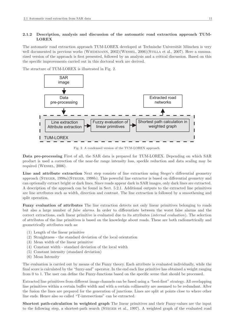
The structure of TUM-LOREX is illustrated in Fig. 2.
Line extractionAttribute extraction
Fuzzy evaluation oflinear primitives
Shortest path calculation inweighted graph
Datapre-processing
Extracted roadnetworks
TUM-LOREX
SARimage
Fig. 2. A condensed version of the TUM-LOREX approach.
Data pre-processing First of all, the SAR data is prepared for TUM-LOREX. Depending on which SAR
product is used a correction of the near-far range intensity loss, speckle reduction and data scaling may be
required (Wessel, 2006).
Line and attribute extraction Next step consists of line extraction using Steger’s differential geometry
approach (Steger, 1998a)(Steger, 1998b). This powerful line extractor is based on differential geometry andcan optionally extract bright or dark lines. Since roads appear dark in SAR images, only dark lines are extracted.
A description of the approach can be found in Sect. 5.2.1. Additional outputs to the extracted line primitives
are line attributes such as width, direction and contrast. The line extraction is followed by a smoothening andsplit operation.
Fuzzy evaluation of attributes The line extraction detects not only linear primitives belonging to roadsbut also a large number of false alarms. In order to differentiate between the worst false alarms and the
correct extractions, each linear primitive is evaluated due to its attributes (internal evaluation). The selection
of attributes of the line primitives is based on the knowledge about roads. These are both radiometrically andgeometrically attributes such as:
(1) Length of the linear primitive(2) Straightness - the standard deviation of the local orientation
(3) Mean width of the linear primitive
(4) Constant width - standard deviation of the local width(5) Constant intensity (standard deviation)
(6) Mean Intensity
The evaluation is carried out by means of the Fuzzy theory. Each attribute is evaluated individually, while the
final score is calculated by the “fuzzy-and” operator. In the end each line primitive has obtained a weight ranging
from 0 to 1. The user can define the Fuzzy-functions based on the specific scene that should be processed.
Extracted line primitives from different image channels can be fused using a “best-first” strategy. All overlappingline primitives within a certain buffer width and with a certain collinearity are assumed to be redundant. After
the fusion the lines are prepared for the generation of junctions. Lines are split at points close to where other
line ends. Hence also so called “T-intersections” can be extracted.
Shortest path-calculation in weighted graph The linear primitives and their Fuzzy-values are the input
to the following step, a shortest-path search (Steger et al., 1997). A weighted graph of the evaluated road

12 2 Previous work
primitives is constructed. In this graph edges correspond to linear primitives and vertices correspond to thestarting and ending points of the linear primitives. The edges become each a final weight (e.g. cost) which is
defined as its length divided by its Fuzzy value. Since the Fuzzy values range from 0 to 1, the final weight of
the highest rated segments (Fuzzy value = 1) will be equal to its length. As the evaluation get closer to 0, thefinal weight approaches ∞.
In general there is a gap between the road segments. In order to fill the gaps, new hypothetic connectingsegments are introduced. The gap length between vertices of not already connected edges are calculated. If
certain criteria are fulfilled a connecting segment is introduced. These are:
(1) The absolute gap length
(2) The relative gap length (compared with the adjacent road segments)
(3) The direction differences between the gap and the adjacent road segments, whereby collinearity (withina road) and orthogonality (e.g., at junctions) are preferred
(4) An additional clipping threshold, which ensures that the weight of a gap cannot become higher than that
of the adjacent road segments
The result of introducing connection hypotheses is an highly oversegmented network which is “cleaned” by
selecting the most significant parts of the network. The selection is based on criteria derived from the functional
properties of roads, i.e. that different places or roads are connected in the scene. This is algorithmically im-plemented as a shortest-path-search in a weighted graph. Here best-valued road segments are selected as seed
points and these are connected by the shortest-path-search through the graph. If road networks eventually have
to cross the image border, road segments next to the image border can be selected manually by a user (Ste-
ger et al., 1997). This heuristic approach is both simple and effective and is especially important for small
sub-urban scenes. The path search is based on the Dijkstra algorithm. An optimal path is selected as part of
the road network if the total length of the path exceeds a certain threshold. This favors a connection betweentwo seed points placed far away from each other.
External evaluation At Technische Universitat Munchen an external evaluation method for comparing theautomatically extracted road networks with reference data was also evolved (Heipke et al., 1997) (Wiedemann,
2002). The evaluation consists of two steps; (1) the extracted network is matched to the reference data and (2)
three quality measures, correctnes, completeness, and root mean square error are calculated.
The matching is carried out by first re-sampling both the reference and the extracted results. The distance
between each point of a line primitive is then equal for both data sets. Extraction points and reference points
are matched to each other given that the points are close and within a certain distance (“buffer”) and that thelocal direction difference between the two is not bigger than a certain threshold. Redundant matching is avoided
by making sure that each point is only matched once.
Completeness gives us an indication of how much of the reference network was actually extracted. It is defined
as the percentage of the reference data which is matched with the extracted network data.
completeness =length of matched reference
length of reference(1)
Correctness tells us how correct the extracted network is and is the percentage of the extracted network whichis matched with the reference data.
correctness =length of matched reference
length of extracted network(2)
RMS tells us the geometrical accuracy of the extracted road data. In general the value varies with the bufferwidth.
RMS − error =
√
√
√
√
n∑
i=1
d2i
n(3)
where di is the distance between the each pair i of matched extraction and reference points.
Analysis and discussion important for this work
The advantage of TUM-LOREX is its well modeled network characteristics (Stilla et al., 2007). Any lineextraction applied to any image data can be the input to the network generation. Therefore the modifications
made for SAR data were mainly concentrated to pre-processing steps. TUM-LOREX has already shown promis-
ing results in terms of road extraction from SAR data, but was still neither adapted nor tested thoroughly for

2.2 Data fusion for automatic object extraction from SAR 13
multi-aspect data. As common for most approaches the line extraction from TUM-LOREX often delivers partlyfragmented and erroneous results. Especially in forest and in urban areas over-segmentation occurs frequently.
Furthermore occlusions due to surrounding objects may cause gaps, which are hard to compensate. One step
to a solution is the use of multi-aspect SAR images. If line extraction fails to detect a road in one SAR view,it might succeed in another view illuminated from a more favorable direction. Therefore multi-aspect images
supply the interpreter with both complementary and redundant information. But due to the over-segmented
line extraction, the information is often contradicting as well. A correct fusion step has the ability to combineinformation from different sensors, which in the end is more accurate and better than the information acquired
from one sensor alone.
Context does not give us direct information about the object of interest but additional information whichhas influence and/or stand in relation to the object of interest (Baumgartner et al., 1997a). Local context
means information about nearby objects such as buildings, trees, traffic signs, which stands in a relation to
the appearance of the road (Baumgartner et al., 1997b). Global context information (e.g. forest, residential,
industrial and rural areas) gives us information about larger image regions where roads have different typicalcharacteristics. Hence global context provides us with a-priori information. As already stated previous work has
shown that local and global context can improve the results obtained by TUM-LOREX. For multi-aspect SAR
data the integration of this information is even more important. Due to the different aspect angle the occlusionsappear very differently. In order to exploit multi-aspect SAR data optimally these occlusions should not only
be detected but also included in the fusion. Naturally the sensor geometry must be included as well.
Hence a fusion module shall be developed which makes use of both sensor geometry information as well ascontext information. The following goals should be achieved:
⋄ To exploit the possibilities of multi-aspect SAR imagery for automatic road extraction.
⋄ To develop a fusion module for multi-aspect SAR data. The fusion shall be implemented in TUM-LOREX.⋄ To extend the integration of local and global context as well as the sensor geometry.
2.2 Data fusion for automatic object extraction from SAR
2.2.1 What is data fusion?
Data fusion techniques are beneficial as soon as data from multiple sensors are combined for making a decision
that is not possible from one sensor alone. Data fusion was in the beginning a research topic for militarypurposes and has been practiced for ocean surveillance, air-to-air defense, battlefield intelligence, and target
acquisition (Hall and Llinas, 2001). Most systems were designed for detection, tracking, and identification of
targets. In recent years, data fusion has been utilized for non-military applications addressing problems such as
implementation of robotics, automated control of industrial manufacturing systems, and medical applications.In the field of remote sensing data fusion has been a current topic for many years. This is due to the extensive
availability of satellite data of the Earth acquired from different sensors. Utilizing the data fusion concept within
remote sensing is hardly something new. However the exact meaning of the term data fusion applied to remotesensing was in the beginning vague and could vary from one researcher to another (Wald, 1999).
Data fusion gives the user a tool for formalizing the approach and for estimating the quality of information during
the fusion process. Furthermore well-known definitions are applied and data fusion scientists working in differentfields are able to cooperate. In fact, data fusion is a multi-disciplinary topic and combines a large number of
methods and mathematic tools, including signal processing, pattern recognition and artificial intelligence. Even
though data fusion has existed for some years, the terminology is not always consistent. For military applications,the Joint Directors of Laboratories (JDL) Data Fusion Working Group has defined a unifying terminology for
data fusion. Their short and concise definition on data fusion is (Steinberg et al., 1998)
“Data fusion is the process of combining data or information to estimate or predict entity states.”
Wald (1998) and Wald (1999) suggested a common formalism for data fusion applied to remote sensing. He
has also written a book entirely about data fusion and remote sensing (Wald, 2002),
Data fusion is a formal framework in which are expressed means and tools for the alliance of data originating
from different sources. It aims at obtaining information of greater quality will depend upon the application.
14 2 Previous work
In remote sensing, data fusion deals with problems such as (Wald, 2002):
⋄ Image data from multiple sensors with different signal properties, such as optical and radar data
⋄ Image data with different spatial and/or temporal resolution
⋄ Image data combined with numerical models representing geophysical/biological processes
The aim of this section is to shortly explain some definitions used in this work, and not to give an introduction
to data fusion. The topic is extensive and there are many good textbooks available (Wald, 2002) (Hall, 1992).
Data fusion definitions
⋄ Measurements represent the output coming from the sensor, in general signals or pixel values. These are
the observations.⋄ Attributes are properties of the object of interest. That can be a color, geometrical measures, or statistical
values such as mean or standard deviation. These are also sometimes called features. However the definition
attributes is better used when fusion is applied to remote sensing, since features is also the definition ofextracted information such as edges, lines, points, etc. Attributes are often gathered in state vectors.
⋄ Associations link observations and make sure that these observations belong to the same entity.
⋄ Rules define relationships between objects and their state vectors. Rules may be mathematical operations,methods or reasoning
⋄ Decisions or with other words, identity declaration result from the application of rules.
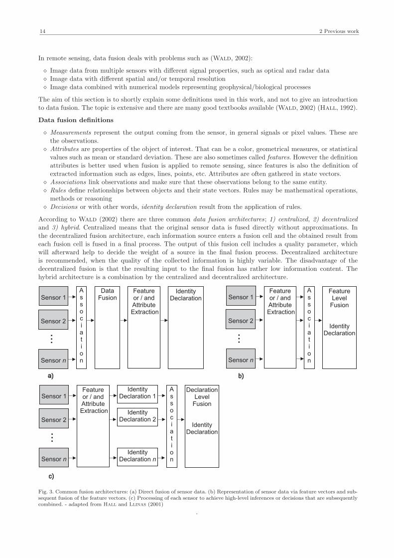
According to Wald (2002) there are three common data fusion architectures; 1) centralized, 2) decentralizedand 3) hybrid. Centralized means that the original sensor data is fused directly without approximations. In
the decentralized fusion architecture, each information source enters a fusion cell and the obtained result from
each fusion cell is fused in a final process. The output of this fusion cell includes a quality parameter, which
will afterward help to decide the weight of a source in the final fusion process. Decentralized architectureis recommended, when the quality of the collected information is highly variable. The disadvantage of the
decentralized fusion is that the resulting input to the final fusion has rather low information content. The
hybrid architecture is a combination by the centralized and decentralized architecture.
Sensor 1Association
DataFusion
Sensor 2
Sensor n
Featureor / andAttributeExtraction
IdentityDeclaration
...
Sensor 1Association
DeclarationLevel
Fusion
IdentityDeclaration
Sensor 2
Sensor n
Featureor / andAttributeExtraction
IdentityDeclaration 1
...
Sensor 1Association
Sensor 2
Sensor n
Featureor / andAttributeExtraction
...
IdentityDeclaration 2
IdentityDeclaration n
FeatureLevel
Fusion
IdentityDeclaration
a)
c)
b)
Fig. 3. Common fusion architectures: (a) Direct fusion of sensor data. (b) Representation of sensor data via feature vectors and sub-sequent fusion of the feature vectors. (c) Processing of each sensor to achieve high-level inferences or decisions that are subsequentlycombined. - adapted from Hall and Llinas (2001)
.

2.2 Data fusion for automatic object extraction from SAR 15
Hall and Llinas (2001) suggests three architectures, whose definitions are more “easy-to-grasp” than thoseproposed by Wald. These are 1) direct fusion of data, 2) representation of sensor data via state vector, or feature
vectors and 3) processing of each sensor to achieve high-level inferences or decisions, which are subsequently
combined (see Fig. 3). The first one is very similar to Wald’s definition of centralized architecture, while thethird one has similarities with the definition of the decentralized fusion.
It is also common within remote sensing fusion to divide the fusion approaches into different levels instead of
architectures. Remote sensing fusion approaches are then classified into three levels; pixel level, feature leveland decision level (Pohl and Van Genderen, 1998) (Zhang, 2010). Pixel-level fusion is regarded as low-
level fusion while feature-level and decision-level are often called high-level fusion. Pixel-level fusion means
that the data is fused at the lowest processing level. Here a centralized (direct fusion) architecture is applied.Feature-level fusion is used when different features such as edges, corners, lines or different texture parameters
are first extracted from each single image. Based on the fused features the following processing takes place.
One can say that the features create a common feature space for the subsequent object classification (Waltz,
2001). Decision level fusions represent the decentralized architecture. Each image is first processed by a certainalgorithm. The output of these algorithms are expressed as decisions or confidences, which are combined in
a following fusion. Decision-level fusion can be applied both to processed pixel information or to processed
extracted features. However important is that the fused pixels or features have obtained decisions or confidencesbefore the subsequent fusion. Sometimes the discrimination between the different fusion levels is diffuse.
2.2.2 Data fusion for man-made object extraction from SAR data - previous work
At first glance better accuracy is obtained by direct fusion of data since the fusing information is closer to
the source and the fusion works on signal level (pixel-level). However, direct fusion on signal level is only
recommendable if the data is commensurate (i.e. the sensors measure the same physical phenomena). Also if aninformation source has a large error rate, it might (depending on the fusion process) damage the outputs of the
fusion. In contrary to multi-spectral optical images, a direct fusion of multi-aspect SAR data on pixel-level must
be handled with much more care. Preferably the statistical and phenomenological properties of SAR image datashall be taken into consideration.
In this section different fusion approaches carried out on pixel-, feature- and decision-level are discussed. We
have mainly concentrated on approaches developed for object extraction from SAR data.
Pixel-level fusion Pixel-level fusion has been applied widely to optical images when multi-spectral and
panchromatic data shall be fused. The aim is to obtain a better spatial resolution, get enhanced structural
and textural details but also to keep the original multi-spectral information, so called pan-sharpening (Zhang,2010), (Weidner and Centeno, 2009). But pixel-level fusion has also been applied to SAR data, mainly for land
use classification. An interesting approach uses pixel-level fusion on SAR and optical data (Lombardo et al.,
2003). First the data is fused on pixel-level, hence resulting in a vector for each pixel with signal response fromeach image. A classification is then carried out by assuming that the data follows a multivariate log-normal
distribution. Pixel-level fusion was also applied to land use classification of RADARSAT images (Asilo et al.,
2007). A fusion on pixel-level using different pixel-level fusion techniques delivered good results, also thanks to
the low resolution and the temporal data obtained by same sensor geometry.
Feature-level fusion Feature-level fusion is often applied to urban SAR remote sensing. For instance it has
been applied to urban area interpretation of TerraSAR-X data (Chaabouni Chouayak and Datcu, 2010).A combination of extracted bright and dark linear features using the line detector as proposed in Tupin et al.
(1998) are fused. Areas are labeled by using geometrical properties as well as contextual properties (i.e. the
combination of high or low frequency of bright and dark linear features). An other interesting topic is building
detection and building height estimation from multi-aspect SAR data. For the grouping of extracted featuresa production system based on perceptual grouping was applied (Soergel et al., 2009). Also for this topic the
viewing geometry of the SAR sensor plays an important role. That is considered for building recognition and
building signature analysis from multi-aspect InSAR data (Thiele et al., 2007)(Thiele et al., 2010). Feature-level fusion is also utilized as soon as several line detectors are combined (Hedman et al., 2008)(Hedman et al.,
2010). The two line extractors used in Hedman et al. (2010) performs differently. One is powerful in rural areas
as the other one performs better in urban areas. Hence urban and rural areas were extracted before the linedetectors were applied. The fusion of the line detectors were carried out by a logical AND operation.
Decision-level fusion Techniques often applied to decision-level fusion are rule-based systems (knowledge-
based methods), fuzzy-theory, Dempster-Shafer’s method and Bayesian theory. An early work dedicated to

16 2 Previous work
Fuzzy-fusion of linear features extracted from SAR data was presented by Chanussot et al. (1999). The aimof this work was to improve the first step of road extraction, the results from a morphological line extractor, by
using multitemporal images. The ability to suppress false alarms and at the same time improve the detection
was tested for different fusion operators, mostly fuzzy operators. Fuzzy-fusion was also applied for buildingdetection (Levitt and Aghdasi, 2000).
Lisini et al. (2006) presents an approach which combines both Markovian and fuzzy-theory. Here the line
segments were assigned a likelihood value (based on a Markovian and fuzzy ARTMAP classifier) before the
fusion. Based on an associative symmetrical sum, also applied in Tupin (2000), the response from each linedetector is merged.
A decision-level fusion for land cover classification of SAR and optical data has been developed. Each single
source is classified by means of support vector machines. The outcome of the support vector machine classifi-
cation is fused testing different fusion techniques such as maximum likelihood, decision trees, boosted decisiontrees, support vector machines, and random forest. Here support vector machines (Waske and Benediktsson,
2007) and random forest (Waske and van der Linden, 2008) showed promising results.
Tupin et al. (1999) proposed a Dempster-Shafer fusion process of several structure detectors. This work is
interesting since it aims to give an overall interpretation of low resolution SAR images. Many cartographicelements such as roads, rivers, urban areas, forest areas, etc. are detected. For this reason different linear features
and larger objects are extracted from the scene. The output of each detector is assigned with a confidence value
that the object belong to certain classes. The reason why Dempster-Shafer is applied in this case is whileDempster-Shafer is able to deal with union of classes. Furthermore some detectors only detect one or only a few
classes. Classical Bayesian theory would require that the operators were able to distinguish all classes. Anyway
Bayesian network theory should be able to deal with a fusion of this kind of information and could have been
an option.
Bayesian network theory has been successfully tested for feature fusion for 3D building description (Kim and
Nevatia, 2003)(Kim and Nevatia, 2004). Line features are extracted from optical data and grouped in rectan-
gles. Hypothesis that the groupings are correct or not are verified by a Bayesian network. Since the number of
images varies an expandable Bayesian network (EBN) is applied. An EBN contains repeatable nodes for variousnumber of image data. Knowledge about semantic relationships among the nodes is included since the EBN has a
causal structure. Hidden nodes are introduced for handling correlation between the nodes. Data fusion based on
Bayesian network theory has been applied in numerous other applications such as vehicle classification (Jung-
hans and Jentschel, 2007), acoustic signals (Larkin, 1998) and land mine detection (Ferrari and Vaghi,
2006).
Fusion applied to road extraction from multi-aspect data An interesting work that has shown the
usefulness of multi-aspect data was presented by Tupin (2000) and Tupin et al. (2002). Here the fusion is carriedout twice on different levels; road networks (i.e. final results) in the end and line segments (i.e. intermediate
results) inside the extraction process. Extracted road networks are merged by using a simple superimposition,
while the fusion of the line segments is more complicated. An initial graph of the line segments detected fromboth images is built. The connection step uses an energy minimization procedure as summarized in Sect. 2.1.1.
The measure from two merged line segments is computed by using a disjunctive operator. The disjunctive
operator is characterized by an indulgent behavior (Bloch, 1996). The results from fusing the intermediateresults are not clearly better than the results from the fusion of the end results. The reason could be that the
displacement caused by layover and shadow regions due to high buildings between two possible line segments is
not considered. The difficulty of correctly including this displacement is pointed out (Tupin, 2000).
Merging extracted TUM-LOREX road networks at the end was also investigated by Hedman et al. (2005a). Asimple fuzzy-fusion strategy which favors roads which are closer to the range direction of the sensor or which were
detected in more than one image was introduced. Each image was first processed by TUM-LOREX, meaning
that the extracted result also underwent the shortest-path calculation, before the fuzzy-fusion was applied. The
fusion strategy was tested on road networks extracted from three multi-aspect images of a small sub-scene (seeFig. 4(a)-(c). The result after fusion can be seen in Fig. 4(d). Those roads close to range direction are marked by
an “R”. Falsely extracted roads are marked by an “F”. The usefulness of multi-aspect data is here exemplified
by the road in the middle marked “R” in Fig. 4(c). On the upper side of the road there is a row of trees. In thefirst two images the road is occluded by shadow and layover but is well detectable in the last one. Since the road
is in this case close to range direction, it obtained a higher rating meaning that it was kept after the fusion. This
test shows that the strategy works well for small uncomplicated scenes. But one should keep in mind that the

2.2 Data fusion for automatic object extraction from SAR 17
Range
R
Range
F
Range
R
R
F
(a) (b)
(c) (d)
Fig. 4. Road networks extracted with TUM-LOREX were fused based on a fuzzy-fusion strategy (Hedman et al., 2005a).TUM-LOREX was first applied to three multi-aspect SAR images (a-c). False alarms are marked by “F” and roads with a fa-vorable direction are marked by “R”. The fused results can be seen in (d).
strategy requires that TUM-LOREX delivers already acceptable results. In addition the fuzzy-functions were
set based on an ad-hoc basis.
Dell’Acqua et al. (2003) used simulated multi-aspect data for testing their approach. Here intermediate
results (line segments extracted separately in each image) were fused by a logical OR, followed by a cutting of
the overlapping segments. Longer segments are preserved.
So far none of the fusions developed for road extraction from multi-aspect data fully exploit the capabilities of
multi-aspect data. Neither the displacement effects nor the SAR specific occlusions are taken into consideration.
Main Conclusions
In account with similar works extracted linear features shall be fused. Furthermore intermediate results shall be
fused meaning that the fusion shall be integrated in the road extraction process. Since we have the problem ofmany gaps and false alarms delivered by the line extraction, the linear features cannot be fused directly. Instead
the features shall obtain an uncertainty value before the fusion. Hence a decision-level fusion shall be applied.
In previous decision-level fusion approaches both numerical and symbolical methods were utilized.
Fuzzy-theory is already used for one part of TUM-LOREX - the internal evaluation. Fuzzy functions of ra-diometric and geometric attributes is used for the selection of good road candidates and for sorting out most
probable false alarms. However the functions must be defined manually by a user and the parameter setting
can be rather time consuming. Including local context and sensor geometry means that the number of fuzzyfunctions would soon be incalculable. Besides the approach is rather heuristic and not applicable for dealing
with the contradicting information extracted from multi-aspect SAR data.
Dempster-Shafer theory is useful when the probabilistic model is incomplete, i.e. when some prior or conditionalprobabilities are missing. Tupin et al. (1999) points out that the evidence theory is applicable when the incoming
information is imprecise, which is often the case with SAR images. But Bayesian theory can better handle causal
probabilities. If most of the probabilities are known, but only some are missing, Bayesian theory allows us toassume reasonable values (Pearl, 1988).
Since TUM-LOREX is based on explicit modeling, the fusion shall also include explicit knowledge. For this
Bayesian networks are especially convenient. Bayesian network theory offers us a probabilistic framework based

18 2 Previous work
on the classical Bayesian inference, but allows us a more flexible structure. Contrary to the undirected Markovrandom fields, Bayesian networks belong to the directed graphs. While Markov graphs are useful for expressing
symmetrical spatial relationships, Bayesian networks define causal relationships (Pearl, 2000). Hence we deal
with relations rather than with signals or objects. In fact, the structure of a Bayesian network has much incommon with human reasoning. The causes (or dependencies) among variables are conveniently described by
a network. Directions of the causes are stated which allow top-down or bottom-up combinations of evidence.
At the same time independencies among variables can be defined, which allows us to simplify the system if avariable has influence on only a small part of the variables. That reduces computational efforts.
The conclusion drawn from this is that Bayesian network is the most suitable framework for this type of fusion.
Hence the aim of this work is to develop a Bayesian network fusion based on a probabilistic model as completeas possible.
Range
Probabilisticmodel
Range
Range
Fusionbased onBayesiannetworktheory
Line extractionAttribute extraction
Line extractionAttribute extraction
Line extractionAttribute extraction
.
.
.
Road NetworkCompletion
Sensorgeometry
Global contextinformation
Uncertaintyassessment
Uncertaintyassessment
Association
Uncertaintyassessment
Multi-aspect SAR data
.
.
.
Probabilisticmodel andreasoning
New fusion module
Fig. 5. The fusion and its implementation in TUM-LOREX is illustrated in the figure. The gray area defines those parts that belongto the fusion developed in this work.
The architecture of the fusion and its implementation in TUM-LOREX is illustrated in Fig. 5. Those parts
belonging to the new fusion module are placed within the gray region.
In summary, the new fusion module shall accommodate for following aspects:
⋄ Analysis and probabilistic modeling of the uncertainty of the incoming information (i.e. linear features)⋄ Probabilistic modeling of roads and their local and global context depending on sensor geometry
⋄ Decision-level fusion implemented as a Bayesian network for solving contradicting and supporting hypotheses

19
3 SAR principles and image characteristics
In this chapter a short summary of the principle and the imaging characteristics of Synthetic Aperture Radar
(SAR) will be given. We focus here on the most essential properties, which are relevant for setting up a correctroad and context model depending on the viewing and sensor geometry. There are excellent textbooks about
SAR, both on the topic of SAR processing (Cumming and Wong, 2005) and of SAR imaging characteris-
tics (Massonnet and Souyris, 2008).
3.1 SAR principles
RADAR is an acronym for Radio Detection and Ranging and is essentially a ranging or distance measuring
device. Radar is an active system and it operates in the wavelength area between 1 m and 1mm (0.3-300GHz). The signal characteristics are controlled and allow the utilization of among others interferometry and
polarization for a range of applications. An additional advantage of RADAR is its ability to operate during
bad weather conditions. Electromagnetic energy with frequencies between 1-15 GHz can practically penetratethrough clouds. For shorter frequencies, SAR K-band, there is an atmospheric loss.
The fundamental principle is that the sensor transmits a short, coherent signal toward the target and detects the
backscattered portion of the signal. By measuring the time delay between the transmission of a pulse and thereception of the backscattered “echo” from different targets, their distance from the radar and thus their location
on a reference surface can be determined. As the sensor platform moves forward, recording and processing of
the backscattered signals builds up a two-dimensional image of the surface.
In remote sensing there are three kinds of different radar systems; altimeters, scatterometers, and imaging radar
systems. In this work we will only consider imaging radar systems. The geometry of an imaging radar system is
quite different from an optical imaging system. A side-looking geometry is applied. The platform travels forwardin the flight direction and transmits a signal oblique to the flight direction (see Fig. 6). The illuminated area
on ground is called footprint or swath. Range refers to the across-track direction perpendicular to the flight
direction, while azimuth refers to the along-track direction parallel to the flight direction. Near-range is theportion of the swath closest to nadir, while far-range is the portion of the swath farthest from nadir. In the
near-range, the local incidence angle is steep relative to the local incidence angle in far-range.
A radar’s spatial resolution is dependent on the specific properties of the microwave radiation and geometricaleffects. Normally we talk about two different resolutions, range and azimuth resolution. Two distinct targets
on the surface will be resolved if their distance is larger than half the pulse length. In fact most SAR sensor
applies the “chirp” method and makes use of a pulse compression by frequency modulation. The range resolution
relates then to the bandwidth of the emitted chirp. The azimuth resolution, however, is limited by the azimuthantenna footprint size. The width of the footprint is proportional to the wavelength and inverse proportional
to the antenna length. Better azimuth resolution is normally achieved by either decreasing the wavelength or
by obtaining a longer antenna. This technique is utilized by real aperture radar (RAR).
Synthetic aperture radar has the ability to synthesize a longer antenna by exploiting the motion of the platform.
The target is then almost continuously illuminated and as a result the target is reconstructed from not one
exposure but from several. In principle the azimuth resolution is a function of the synthetic antenna lengthand the distance to the object is no longer relevant. A shorter real antenna length results in a longer simulated
antenna length, which in turn results in a better resolution. An upper band is given, however, by the pulse
repetition frequency. In addition, the design of the real antenna length is restricted by the antenna gain.Nonetheless SAR systems, in contrast to RAR systems, are especially suitable as flight- or space-borne sensors.
The generation of SAR images based on the recorded pulse or chirp echoes is a complicated task. Nowadays it
is operational implemented involving standardized advanced signal processing.

20 3 SAR principles and image characteristics
Flight direction -Azimuth
FootprintFootprint
Range
Near-range
Far-range
θ
Nadir
Local incidenceangle
Fig. 6. Side-looking geometry of a SAR-sensor.
3.2 SAR image characteristics
3.2.1 Geometrical effects
The radar measures the distance to features rather in slant range than the true horizontal distance along the
ground (ground range). This results in varying image scale moving along the image line from near to far range.Targets in near range tend to appear compressed relative to the far range. This effect is dependent on the flight
height and is larger for air-borne systems than for space-borne systems.
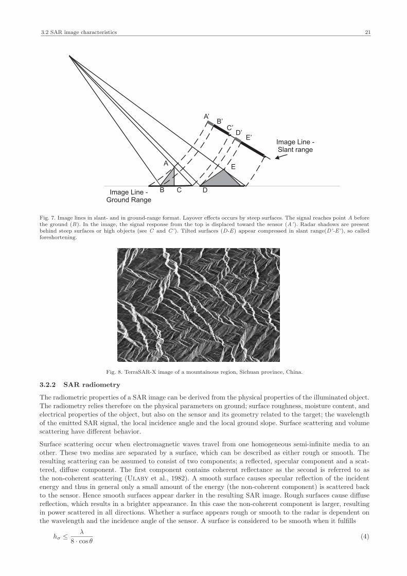
An image in slant range can be transformed into ground range format by using trigonometry. Furthermore,
the side-looking geometry of the SAR sensor results in certain geometric distortions on the resultant imagery.
Shadow, layover and foreshortening are all SAR-specific effects, which occur as soon as high-elevated objectsoccur on the ground surface (see Fig. 7). These effects cannot be compensated for without additional information
but gives clues for the presence of important 3D features.
Foreshortening give rise to a compressed appearance of high objects tilted toward the sensor. The length ofthe slope will be represented incorrectly and give rise to a bright feature in the resulting image. Foreshortening
is dependent on the incidence angle of the sensor and the steepness of the slope. The steeper slope the more
significant is the distortion.
Layover occurs by smaller incidence angles (e.g. in near-range), by steep mountains and by building fronts. In
this case, the radar beam reaches the top of the target before it reaches the ground. As a result, the signal
response from the top is displaced toward the sensor from its true position on the ground and overlayed ontothe echoes from the ground.
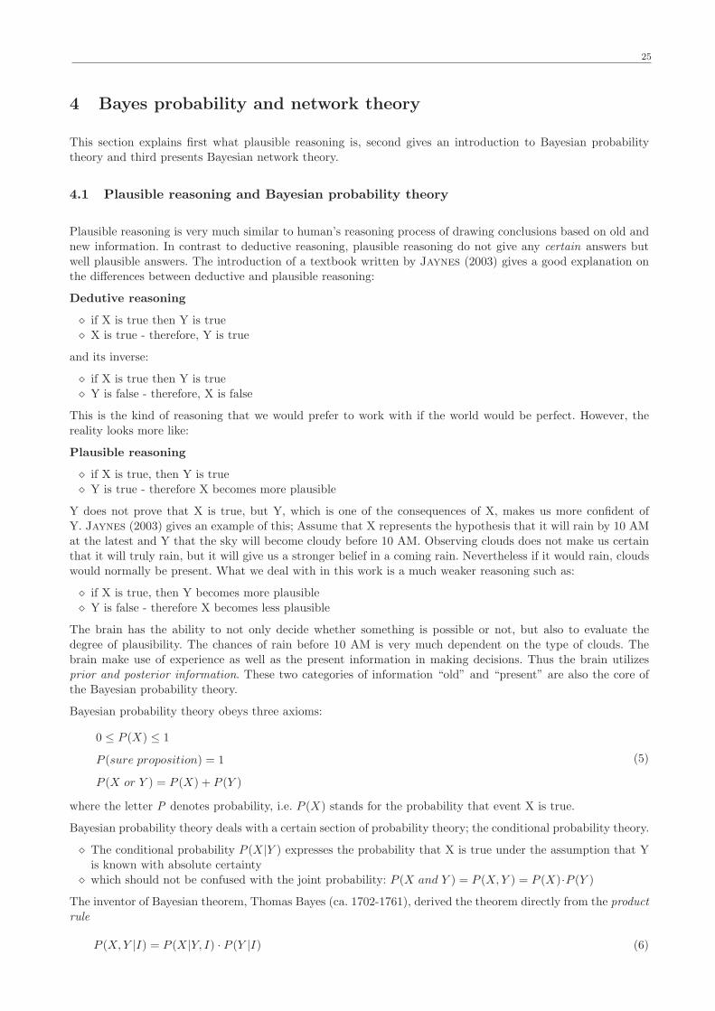
As soon as layover and foreshortening effects are present, radar shadows are present as well. Shadows occurbehind high-elevated objects or steep surfaces, as the radar beam is not able to illuminate the ground surface.
In these areas there are no backscattered signal and they appear black in the image. The strong layover and
shadow regions of a mountainous region can be seen in Fig. 8.
3.2 SAR image characteristics 21
Image Line -Ground Range
Image Line -Slant range
A
B C
B’C’
A’
D’
D
E’
E
Fig. 7. Image lines in slant- and in ground-range format. Layover effects occurs by steep surfaces. The signal reaches point A beforethe ground (B). In the image, the signal response from the top is displaced toward the sensor (A’). Radar shadows are presentbehind steep surfaces or high objects (see C and C’). Tilted surfaces (D-E) appear compressed in slant range(D’-E’), so calledforeshortening.
Fig. 8. TerraSAR-X image of a mountainous region, Sichuan province, China.
3.2.2 SAR radiometry
The radiometric properties of a SAR image can be derived from the physical properties of the illuminated object.
The radiometry relies therefore on the physical parameters on ground; surface roughness, moisture content, and
electrical properties of the object, but also on the sensor and its geometry related to the target; the wavelength
of the emitted SAR signal, the local incidence angle and the local ground slope. Surface scattering and volumescattering have different behavior.
Surface scattering occur when electromagnetic waves travel from one homogeneous semi-infinite media to an
other. These two medias are separated by a surface, which can be described as either rough or smooth. The
resulting scattering can be assumed to consist of two components; a reflected, specular component and a scat-tered, diffuse component. The first component contains coherent reflectance as the second is referred to as
the non-coherent scattering (Ulaby et al., 1982). A smooth surface causes specular reflection of the incident
energy and thus in general only a small amount of the energy (the non-coherent component) is scattered backto the sensor. Hence smooth surfaces appear darker in the resulting SAR image. Rough surfaces cause diffuse
reflection, which results in a brighter appearance. In this case the non-coherent component is larger, resulting
in power scattered in all directions. Whether a surface appears rough or smooth to the radar is dependent onthe wavelength and the incidence angle of the sensor. A surface is considered to be smooth when it fulfills
hσ ≤ λ
8 · cos θ(4)

22 3 SAR principles and image characteristics
The variable hσ represents the surface height variation as defined in (Ulaby et al., 1982). Models describingrough scattering normally consider the height variation not only in vertical direction but also in horizontal
direction.
A tilted surface toward the sensor appears brighter as a result of a stronger reflected signal. This effect is ratherof a specular nature and can be described by a facet model. It is then assumed that the illuminated ground to
consist of several flat facets. Each one of these facets has a local ground slope.
Targets, who consist of two or more perpendicular surfaces, give rise to so-called double bounce or trihedral
bounce scattering (see Fig. 9). Objects with this property (buildings, walls, etc) are sometimes called corner
reflector and are common in urban environments. Metallic objects cause an other kind of strong signal. Due
to their high dielectric constant these objects get a re-radiation pattern the same as an antenna causing anresonant effect.
The dielectric constant describes the resistance to the penetration of electromagnetic waves. The moisture
content plays here a significant role and contributes more than the texture of the material. The penetrationdepth is also wave-length dependent. SAR sensors with larger wavelength (such as L-Band) has the ability to
penetrate cm/m through snow or soil.
Volume scattering has a different nature than surface scattering (see Fig. 9). Volume scattering is caused when
electromagnetic waves propagate through a cloud of scattering elements, each with different dielectric properties,
size, and shape. The spatial locations of these elements are random. Hence, in contrary to surface scattering, the
media is assumed to inhomogeneous. Volume scattering is often very difficult to predict. Often it is hard to findthe boundary when volume scattering and when surface scattering occur. As matter of fact, electromagnetic
interaction with materials with a low dielectric constant and hence a large penetration depth may be better
described by the volume scattering model. Furthermore, both surface and volume scattering often contributesto the scattering from vegetation.
Fig. 9. Strong scattering caused by metallic objects and by double bounce and trihedral bounce reflections can be seen in the leftpart of the image. This industrial area contain large buildings. The right part show the irregular volume scattering caused by highvegetation.
Beyond the physical properties of the object, the so-called speckle effect has a significant impact on the ra-
diometry of the image. Speckle is caused by random constructive and destructive interference from the multiple
scattering returns that will occur within each resolution cell (Massonnet and Souyris, 2008). If the returningwaves within one resolution cell behave constructively, the pixel appears brighter. Destructive interference is
the opposite extreme and results in lower pixel intensity. Speckle has the same behavior as multiplicative noise,
i.e. its variance increases linearly with the mean intensity. High resolution SAR sensors (about 1 m resolution)
show less speckle effect simply since a smaller resolution cell is assumed to have a limited number of scatterers.
Speckle can be reduced by applying speckle filters such as the multiplicative speckle model-based Frost-Filter,
Lee-Filter, and Kuan-Filter and product model-based Gamma MAP filter (Touzi, 2002). An other way ofdecrease the speckle-effect is to apply multi-look processing. A set of samples illuminating the same area are
averaged in power together to produce a smoother image. Each sample is produced by using different parts of
the synthetic aperture. The speckle is in the end reduced but at the cost of a worse resolution.

3.2 SAR image characteristics 23
3.2.3 SAR systems and their data
The data used in this work was acquired by an air-borne (E-SAR) and a space-borne (TerraSAR-X) SAR
system.
The E-SAR system is a multi-frequency, air-borne SAR system, which was developed by the German Aerospace
Center (DLR) in the 90’s. The aim of the research project was to get know-how in SAR sensor design anddata processing techniques for the support to space missions such as ERS-1 and SIR-C/X-SAR. E-SAR is
able to operate in several bands (P-,L-,C- and X Band) (Horn, 1996). A sub-image in X-band can be seen
in Fig. 10. The systems has both polarimetric and interferometric modes. A multi-look processor is integratedin the system, enabling multi-look data up to 8 looks. The experience gained from E-SAR was useful for the
following space-mission TerraSAR-X.
Fig. 10. Sub-image (X-band) acquired by the E-SAR sensor showing parts of the airport in Oberpfaffenhofen, close to Munich,Germany.
Fig. 11. The football stadium Allianz-Arena can be seen in this TerraSAR-X sub-image. The imaging mode is high-resolutionspotlight mode and the data was obtained as radiometrically enhanced data product.
TerraSAR-X is a German space-borne SAR-mission, partly with commercial and partly with scientific in-
terests, developed by the German Ministry of Education and Science (BMBF), DLR and the Astrium
GmbH (Roth et al., 2005). The satellite was launched on 15 June 2007 from the Kazakhstan. The sensoroperates in X-band and has a steerable antenna. This enables a range of imaging modes (Fritz, 2007):
⋄ Stripmap mode - the basic SAR imaging mode with 3.3 m (azimuth resolution)
⋄ Spotlight mode - A phased array beam steering in azimuth direction and thereby increasing the size of the
synthetic aperture, resulting in a resolution in azimuth down to 1.7 m. The drawback of this technique isthe reduced swathwidth.
⋄ High Resolution Spotlight mode with a higher beam steering velocity than the normal spotlight mode
(azimuth resolution down to 1.1 m)

24 3 SAR principles and image characteristics
⋄ ScanSAR mode A wider swath is obtained by switching the antenna elevation steering subsequently andscanning several adjacent ground sub-swaths with different incidence angles. In this way the azimuth reso-
lution is reduced to 18.5 m.
All imaging modes have single and dual polarization modes except ScanSAR mode that has single polarizationmode. Furthermore spatially and radiometrically enhanced data products are available. Multilook processing
and geometric projections such as geocoded ellipsoid correction (assuming one average terrain height) and
enhanced ellipsoid correction (using a digital elevation model (DEM)) can be ordered for ground range data.Side-lobe suppression which is especially important in urban areas is applied.
An example of TerraSAR-X data can be seen in Fig. 11.
25
4 Bayes probability and network theory
This section explains first what plausible reasoning is, second gives an introduction to Bayesian probability
theory and third presents Bayesian network theory.
4.1 Plausible reasoning and Bayesian probability theory
Plausible reasoning is very much similar to human’s reasoning process of drawing conclusions based on old and
new information. In contrast to deductive reasoning, plausible reasoning do not give any certain answers butwell plausible answers. The introduction of a textbook written by Jaynes (2003) gives a good explanation on
the differences between deductive and plausible reasoning:
Dedutive reasoning
⋄ if X is true then Y is true
⋄ X is true - therefore, Y is true
and its inverse:
⋄ if X is true then Y is true
⋄ Y is false - therefore, X is false
This is the kind of reasoning that we would prefer to work with if the world would be perfect. However, the
reality looks more like:
Plausible reasoning
⋄ if X is true, then Y is true
⋄ Y is true - therefore X becomes more plausible
Y does not prove that X is true, but Y, which is one of the consequences of X, makes us more confident of
Y. Jaynes (2003) gives an example of this; Assume that X represents the hypothesis that it will rain by 10 AM
at the latest and Y that the sky will become cloudy before 10 AM. Observing clouds does not make us certain
that it will truly rain, but it will give us a stronger belief in a coming rain. Nevertheless if it would rain, cloudswould normally be present. What we deal with in this work is a much weaker reasoning such as:
⋄ if X is true, then Y becomes more plausible
⋄ Y is false - therefore X becomes less plausible
The brain has the ability to not only decide whether something is possible or not, but also to evaluate the
degree of plausibility. The chances of rain before 10 AM is very much dependent on the type of clouds. The
brain make use of experience as well as the present information in making decisions. Thus the brain utilizesprior and posterior information. These two categories of information “old” and “present” are also the core of
the Bayesian probability theory.
Bayesian probability theory obeys three axioms:
0 ≤ P (X) ≤ 1
P (sure proposition) = 1
P (X or Y ) = P (X) + P (Y )
(5)
where the letter P denotes probability, i.e. P (X) stands for the probability that event X is true.
Bayesian probability theory deals with a certain section of probability theory; the conditional probability theory.
⋄ The conditional probability P (X|Y ) expresses the probability that X is true under the assumption that Y
is known with absolute certainty⋄ which should not be confused with the joint probability: P (X and Y ) = P (X,Y ) = P (X)·P (Y )
The inventor of Bayesian theorem, Thomas Bayes (ca. 1702-1761), derived the theorem directly from the product
rule
P (X,Y |I) = P (X|Y, I) · P (Y |I) (6)
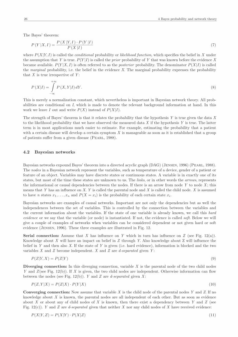
26 4 Bayes probability and network theory
The Bayes’ theorem:
P (Y |X, I ) =P (X |Y, I ) · P (Y |I )
P (X |I )(7)
where P (X|Y, I) is called the conditional probability or likelihood function, which specifies the belief in X under
the assumption that Y is true. P (Y |I) is called the prior probability of Y that was known before the evidence Xbecame available. P (Y |X, I) is often referred to as the posterior probability. The denominator P (X|I) is called
the marginal probability, i.e. the belief in the evidence X. The marginal probability expresses the probability
that X is true irrespective of Y :
P (X|I) =
+∞∫
−∞
P (X,Y |I) dY . (8)
This is merely a normalization constant, which nevertheless is important in Bayesian network theory. All prob-
abilities are conditional on I, which is made to denote the relevant background information at hand. In this
work we leave I out and write P (X) instead of P (X|I).
The strength of Bayes’ theorem is that it relates the probability that the hypothesis Y is true given the data X
to the likelihood probability that we have observed the measured data X if the hypothesis Y is true. The latter
term is in most applications much easier to estimate. For example, estimating the probability that a patientwith a certain disease will develop a certain symptom X is manageable as soon as it is established that a group
of patients suffer from a given disease (Pearl, 1988).
4.2 Bayesian networks
Bayesian networks expound Bayes’ theorem into a directed acyclic graph (DAG) (Jensen, 1996) (Pearl, 1988).The nodes in a Bayesian network represent the variables, such as temperature of a device, gender of a patient or
feature of an object. Variables may have discrete states or continuous states. A variable is in exactly one of its
states, but most of the time these states are unknown to us. The links, or in other words the arrows, representsthe informational or causal dependencies between the nodes. If there is an arrow from node Y to node X ; this
means that Y has an influence on X. Y is called the parental node and X is called the child node. X is assumed
to have n states x1, . . . , xn and P (X = xi) is the probability of each certain state xi.
Bayesian networks are examples of causal networks. Important are not only the dependencies but as well the
independences between the set of variables. This is controlled by the connection between the variables and
the current information about the variables. If the state of one variable is already known, we call this hardevidence or we say that the variable (or node) is instantiated. If not, the evidence is called soft. Below we will
give a couple of examples of networks when variables can be considered dependent or not given hard or soft
evidence (Jensen, 1996). These three examples are illustrated in Fig. 12.
Serial connection: Assume that X has influence on Y which in turn has influence on Z (see Fig. 12(a)).
Knowledge about X will have an impact on belief in Z through Y. Also knowledge about Z will influence the
belief in Y and then also X. If the state of Y is given (i.e. hard evidence), information is blocked and the twovariables X and Z become independent. X and Z are d-separated given Y :
P (Z|Y,X) = P (Z|Y ) (9)
Diverging connection: In this diverging connection, variable X is the parental node of the two child nodes
Y and Z (see Fig. 12(b)). If X is given, the two child nodes are independent. Otherwise information can flowbetween the nodes (see Fig. 12(b)). Y and Z are d-separated given X :
P (Z, Y |X) = P (Z|X) · P (Y |X) (10)
Converging connection: Now assume that variable X is the child node of the parental nodes Y and Z. If no
knowledge about X is known, the parental nodes are all independent of each other. But as soon as evidence
about X or about any of child nodes of X is known, then there exist a dependency between Y and Z (seeFig. 12(c)). Y and Z are d-separated given that neither X nor any child nodes of X have received evidence:
P (X|Y,Z) = P (X|Y ) · P (X|Z) (11)

4.2 Bayesian networks 27
ZY
X
a)
Y ZX
X
Y Z
b) c)
Fig. 12. Bayesian networks with: (a) serial connection, (b) diverging connection, (c) converging connection.
If two nodes are not d-separated, they are called d-connected.
The mathematical definition of Bayesian networks is as follows (Jensen, 1996)(Pearl, 1988)
The Bayesian network U is a set of nodes U = {X1, ..., Xn}, which are connected by a set of arrows A =
{(Xi, Xj) |Xi, Xj ∈ U, i 6= j}. Let P (u) = P (x1, . . . , xn) be the joint probability distribution of the state valuesx. Lowercase letters stand for particular values (e.g. TRUE or FALSE). For being a Bayesian network, U
has to satisfy the Markov condition, which means that a variable must be conditionally independent of its
nondescendents given its parents. P (x1, x2, ..., xn) can therefore be defined as
P (x1, x2, ..., xn) =
n∏
i=1
P (xi|pa(Xi)) (12)
where pa(Xi) represent the parents states of node Xi. If this node has no parents, the prior probability P (Xi =
xi) must be specified.
Assume a Bayesian network composed by two child nodes, X and Z, and one parental node, Y (see Fig. 13).Since X and Z are considered to be independent given the variable Y, the joint probability distribution P(y,x,z)
can be expressed as
P (y, x, z) = P (y)P (x |y )P (z |y ) (13)
Fig. 13. A Bayesian network with one parental node (Y ) and its two child nodes (X and Z ) and their corresponding conditionalprobabilities.

28 4 Bayes probability and network theory
4.2.1 Belief propagation in Bayesian networks
Until now the Bayesian network has been described as the joint probability of all variables contained in the
network (see Eq. 13). However in many applications one is interested in the probability related to one variable,the hypothesis variable. Hypothesis variables are normally impossible to observe, but are the variables with the
states we would like to estimate. The estimation is done by means of known or partly known states of observable
variables, the information variables. Pearl (1988) describes a belief updating system which will be applied inthis work. In this system each variable will obtain a processor, which controls the information running from
one variable to its neighboring variables. Information run only via the links and these links are supposed to be
always open.
The evidence arriving to an information node in such a system may be sent from both neighboring parental and
child nodes at the same time. Information coming from a parent, e+ is named causal or predictive evidence.
Predictive information propagates in a top-down direction. Information from child nodes, e−, flow in the oppositedirection and is called diagnostic evidence. Information coming from the top (the parents) and from the bottom
(the children) are differentiated and therefore expressed by different Greek letters (see Fig. 14):
π(x) = P (x∣
∣e+ ) (14)
and
λ(x) = P (e− |x ) (15)
The total belief in node X is obtained by fusing evidence coming from the top and from the bottom:
BEL(x) = α λ(x) π(x) (16)
where α is a normalizing constant assuring thatN∑
i=1
BEL(xi) = 1 for all n states x of X.
Each arrow between two nodes (X → Y ) is quantified by conditional probability functions. Probability functionsin a Bayesian network can have a countable (discrete) or a continuous set of states. Conditional probabilities
for discrete states are usually realized by conditional probability tables. Conditional probabilities for continuous
states can be estimated by probability density functions.
By such tables’ definition, the nodes in a Bayesian network are variables with a finite number of mutually
exclusive states. If the variable X has states x1 . . . xn and the variable Y has states y1 . . . ym then MY |X is an
mxn table containing numbers P (yi|xj) such as
MY |X = p (Y = y |X = x ) =
p(y1 |x 1) p(y1 |x2
) . . . p(y1 |xn)
p(y2 |x 1) p(y2 |x2
) p(y2 |xn)
......
...
p(ym |x1) p(ym |x
2) · · · p(ym |xn)
(17)
The sum of the columns should preferably be one.
ZY
e+
e-
π( )y
λ( )z
X
π( )x
λ( )y
Fig. 14. The belief update is illustrated for a serial connection.

4.2 Bayesian networks 29
Assume a Bayesian network consisting of one parental node X and two child nodes Y and Z (see Fig. 14).Assume that evidence arrive at node X, some prior information expressed by the vector π(x). Node Y is not
observed directly but is supported by node Z, which state is observed, e− {Z = zobserved}. This information
propagates to node Y and then later to node X. Based on this information λ(y) can be estimated. The statesin node Y is not known for sure, but the vector λ(y) contains for each state of Y an uncertainty value entirely
based on Z. The belief in node X can the be expressed as:
BEL(x) = α λ(x)π(x) = αMY |X λ(y)π(x) (18)
where
λ(x) = MY |X λ (y) (19)
is a matrix product.
More detailed information on Bayesian network theory can be found in Jensen (1996) and in Pearl (1988).
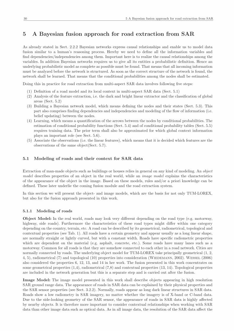
30 5 A Bayesian fusion approach for road extraction from SAR
5 A Bayesian fusion approach for road extraction from SAR
As already stated in Sect. 2.2.2 Bayesian networks express causal relationships and enable us to model data
fusion similar to a human’s reasoning process. Hereby we need to define all the information variables andfind dependencies/independencies among them. Important here is to realize the causal relationships among the
variables. In addition Bayesian networks requires us to give all its entities a probabilistic definition. Hence an
underlying probabilistic model as complete as possible must be found. That means that all incoming informationmust be analyzed before the network is structured. As soon as the correct structure of the network is found, the
network shall be learned. That means that the conditional probabilities among the nodes shall be estimated.
Doing this in practice for road extraction from multi-aspect SAR data involves following five steps:
(1) Definition of a road model and its local context in multi-aspect SAR data (Sect. 5.1)(2) Analysis of the feature extraction, i.e. the dark and bright linear extractor and the classification of global
areas (Sect. 5.2)
(3) Building a Bayesian network model, which means defining the nodes and their states (Sect. 5.3). Thispart also comprises finding dependencies and independencies and modeling of the flow of information (i.e.
belief updating) between the nodes.
(4) Learning, which means a quantification of the arrows between the nodes by conditional probabilities. Theestimation of conditional probability functions (Sect. 5.4) and of conditional probability tables (Sect. 5.5)
requires training data. The prior term shall also be approximated for which global context information
plays an important role (see Sect. 5.6).
(5) Associate the observations (i.e. the linear features), which means that it is decided which features are theobservations of the same object(Sect. 5.7).
5.1 Modeling of roads and their context for SAR data
Extraction of man-made objects such as buildings or houses relies in general on any kind of modeling. An object
model describes properties of an object in the real world, while an image model explains the characteristics
of the appearance of the object in the image. Based on these models, rules and/or a priori knowledge can bedefined. These later underlie the coming fusion module and the road extraction system.
In this section we will present the object- and image models, which are the basis for not only TUM-LOREX,
but also for the fusion approach presented in this work.
5.1.1 Modeling of roads
Object Model: In the real world, roads may look very different depending on the road type (e.g. motorway,
highway, side roads). Furthermore the characteristics of these road types might differ within one category
depending on the country, terrain, etc. A road can be described by its geometrical, radiometrical, topological andcontextual properties (see Tab. 1). All roads have a certain geometry and appear usually as a long linear shape,
are normally straight or lightly curved, but with a constant width. Roads have specific radiometric properties
which are dependent on the material (e.g. asphalt, concrete, etc.). Some roads have many lanes such as amotorway. Common for all roads is that they are somehow connected to each other in a road network. Cities are
normally connected by roads. The underlying object model for TUM-LOREX take principally geometrical (1, 2,
4, 5), radiometrical (7) and topological (10) properties into consideration (Wiedemann, 2002). Wessel (2006)also considered the properties 6, 12, 13, and 14 in her work. The fusion presented in this work concentrates on
some geometrical properties (1,4), radiometrical (7,8) and contextual properties (13, 14). Topological properties
are included in the network generation but this is a separate step and is carried out after the fusion.
Image Model: The image model presented in this work shall describe objects appearing in high resolutionSAR ground range data. The appearance of roads in SAR data can be explained by their physical properties and
the SAR sensor properties (see Sect. 3.2.2). Normally, roads appear as long dark linear structures in SAR data.
Roads show a low radiometry in SAR imagery, no matter whether the imagery is of X-band or C-band data.Due to the side-looking geometry of the SAR sensor, the appearance of roads in SAR data is highly affected
by nearby objects. It is therefore more important to consider contextual relationships when working with SAR
data than other image data such as optical data. As in all image data, the resolution of the SAR data affect the

5.1 Modeling of roads and their context for SAR data 31
Geometrical Properties:
1. Roads have a long, linear shape
2. In general roads have a constant width
3. Roads have parallel edges
4. In general, roads feature a low curvature
5. Roads show a typical width (dependent on the road type)
6. Roads are normally flat with low or no inclination
Radiometrical Properties:
7. Roads consist of homogeneous materials such as asphalt, concrete or gravel
8. The surface of roads can be considered to be smooth
9. Roads are stationary objects
Topological Properties:
10. Roads are usually connected in a network
11. Roads end with a connection or as a dead end
Contextual Properties:
12. Roads connect cities
13. Roads feature a relation to nearby objects (local context)
14. In different surroundings (global context), the appearance of roads differs
Tab. 1. Characteristics of the object model for roads - adapted from (Wessel, 2006).
appearance of roads as well. In low resolution SAR data, roads tend to look like long lines, as in high resolution
SAR data, separate lanes, crash barriers and traffic lights may be discerned. Due to the strong impact causedby nearby objects, the road appearance differ due to the surrounding area (e.g. global context).
5.1.2 Modeling of context
Local context represents all objects that have direct influence on the geometrical and radiometrical properties.
Examples of local context are buildings, high vegetation such as trees, big traffic signs and traffic lights, and
moving vehicles. Buildings and high vegetation cause typically shadow and layover effects. Traffic signs, trafficlights, buildings and all sorts of metallic objects causes strong reflections. These effects may occlude the road
and hinder important road information. The extent of the occlusion depends on the position of the road in
relation to the SAR sensor as well as the type of the local context object on the surface.
In this work we are on one hand interested in the influence of local context on the appearance of road in theimage but on the other hand also in the identification of different local objects. Identification of local context
alone is a good evidence in case of conflicting hypotheses. Therefore the first part is about the relation between
local context objects and the road (i.e. in the image model) and the second part is about how different localcontext objects look like in the SAR image.
Including Shadow and and Layover in the Road Image Model
Shadow and layover effects are present as soon as high objects are present. The extent of the effect in ground
range data depends on the local incidence angle θ, the height of the target (H ) and the slope of the targetsurface. In Fig. 15, the length of a shadow S and a layover L of a tree is depicted. Assuming a horizontal
reference surface and an image in ground range the length of the shadow, S :
S = H · tan θ (20)
and the length of the layover, L:
L = H · cot θ. (21)
The shadow and layover effects raised by an object vary with the location of the object in relation to the positionof the SAR sensor. Roads are preferably located in range direction to get the best possible visibility. The shadow
lengths projected to the normal of the road Sn can be expressed as
Sn = H · tan θ · sin β (22)

32 5 A Bayesian fusion approach for road extraction from SAR
q
s
b
ssN
wR
a
Range
H
S <WN R
b
s
a
W <S <WR N NoL
b=90°
a
S >WN NoL
sN
sN w
Rw
R
L
q
b wR
a
L <(WN R-W )Min
LN L
L >(W -W )N R Minb
a
wR
LN
L
Fig. 15. The shadow and layover effects caused by a row of trees is depicted first as a side view. The shadow regions are illustratedthree times and the layover two times as top view for different β angles. The length of the occlusions, S and L, stays the same,but the occlusions projected as normal to the road, Sn and Ln, increases as soon as the β angle increase. WR is the assumedwidth of the road and WNoL is the maximum width for the line extraction, which is a parameter that has to be set during the lineextraction.
and the layover:
Ln = H · cot θ · sinβ (23)
where β is the angle between the range direction and the direction of the road. In this work, β is called the roadvisibility angle (Hedman et al., 2005b). The larger β is, the higher is the probability that the road is occluded
by a shadow or a layover.
Objects Located at One Side When trees or houses are located at just one side of the road, either layover
or shadow might occlude parts of the road. Depending on β, the height of the object, H, and the width of the
road WR, the road can either be partly or completely covered. If the shadow cover only a little part of theroad, the linear shape is kept and the road show about the same characteristics as a road without any high
objects nearby in the SAR image (see Fig. 16). Hence, in favorable cases the road has kept its linear shape and
is likely to be detected by a line extraction. If β increases further the road can be completely covered. If thelinear shape is kept, it still might be detected but shows then the characteristics of a shadow, meaning that the
backscattered intensity is almost zero. If β approaches 90◦ the width of the shadow region is likely to exceed
the width parameter set by the line extraction and is hence not detected by the line extraction.
If a road of width 10 m is bordered by 15 m high trees on one side and is viewed by a SAR sensor with a
local incidence angle of 45◦, then the road is totally covered by the shadow for road visibility angles largerthan 42◦(see Tab. 2). For less β angles the shadow occludes only a part of the road and can be viewed for the
extraction as a part of the road itself. The maximum road visibility angle for which the road is still detectable
is called βmax.
The main problem by layover effects is the decrease of the road width. Even though parts of the road are visible,
the width of the remaining road pixels is below the width limitations for road extraction (WR). Hence, roads
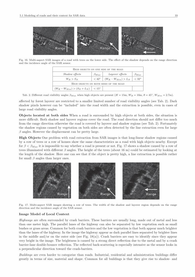
5.1 Modeling of roads and their context for SAR data 33
Range RangeRange
Fig. 16. Multi-aspect SAR images of a road with trees on the lower side. The effect of the shadow depends on the range directionand the incidence angle of the SAR sensor.
High objects on one side of the road
Shadow effects βMax Layover effects βMax
WR > SN < 42◦ (WR − WMin) > LN < 32◦
High objects on both sides of the road
(WR − WMin) > (SN + LN ) < 15◦
Tab. 2. Different road visibility angles βMax when high objects are present (H = 15m, WR = 10m, θ = 45◦, WMin = 2.7m).
affected by forest layover are restricted to a smaller limited number of road visibility angles (see Tab. 2). Dark
shadow pixels however can be “included” into the road width and the extraction is possible, even in cases oflarge road visibility angles.
Objects located at both sides When a road is surrounded by high objects at both sides, the situation is
more difficult. Both shadow and layover regions cover the road. The road direction should not differ too much
from the range direction otherwise the road is covered by layover and shadow regions (see Tab. 2). Fortunatelythe shadow regions caused by vegetation on both sides are often detected by the line extraction even for large
β angles. However the displacement can be pretty large.
High Objects One problem with road extraction from SAR images is that long-linear shadow regions caused
by a row of trees or a row of houses show the same characteristics as a road with high objects nearby. Exceptfor β < βMax it is impossible to say whether a road is present or not. Fig. 17 shows a shadow caused by a row of
trees illuminated with different β angles. The height of the trees (about 16 m) could be estimated by looking at
the length of the shadow. Here one can see that if the object is pretty high, a line extraction is possible rather
for small β angles than larger ones.
Range RangeRange
Fig. 17. Multi-aspect SAR images showing a row of trees. The width of the shadow and layover region depends on the rangedirection and the incidence angle of the SAR sensor.
Image Model of Local Context
Highways are often surrounded by crash barriers. These barriers are usually long, made out of metal and less
than one meter high. The parallel lanes of the highway can also be separated by low vegetation such as small
bushes or grass areas. Common for both crash barriers and the low vegetation is that both appear much brighterthan the lanes of the highway. In the image the highway appear as dark parallel lines separated by brighter lines
in the middle and/or on the outer side (see Fig. 18(a)). Crash barriers are easy to identify since they appear
very bright in the image. The brightness is caused by a strong direct reflection due to the metal and by a crashbarrier-lane double-bounce reflection. The reflected back-scattering is especially intensive as the sensor looks in
a perpendicular direction toward the crash-barriers.
Buildings are even harder to categorize than roads. Industrial, residential and administration buildings differ
greatly in terms of size, material and shape. Common for all buildings is that they give rise to shadow- and

34 5 A Bayesian fusion approach for road extraction from SAR
layover regions as well as strong double-bounce reflections. The main contributors to the total backscatteringin the image are: 1) direct backscattering from the roof, 2) direct backscattering from the wall, 3) direct
backscattering from the ground, 4) wall-ground double-bounce scattering (Stilla and Soergel, 2006) (see
Fig. 18(b)). The signal response from the roof can be both weak and strong depending on the roof structure.A gabled roof oriented perpendicular to range leads to a strong direct reflection which position in the image is
affected by layover. A smooth and flat roof causes a specular reflection away from the sensor. The double-bounce
reflections between the ground and the wall leads to a strong signal response, which occur at the position of thewall. As soon as buildings stand closer to each other the complexity arises due to mixed backscattered signals
from several buildings. If the heights of the buildings vary, high buildings may totally occlude small buildings.
Differentiation between layover and shadow regions becomes more and more complicated.
As the resolution of the SAR sensor improves, the amount of strong backscatterers increases and become more
and more dominant in the image. These are a result of the direct specular reflection due to metallic objectsas window details, balconies, roof details, etc. A detailed description of complicated building shapes in SAR
images is a hard task and include both geometrical (even fine details) and electromagnetic properties of the
building (Guida et al., 2008).
Higher vegetation (i.e. trees) is characterized by an overall medium backscattering intensity. The total backscat-
tering for a radar resolution cell is a result of several backscattering components. According to the forest modeldescribed in the work of Sun and Ranson (1995), which is also presented in Wessel (2006), there are five
main components: 1) direct crown backscatter (i.e. volume scattering), 2) direct backscattering from ground,
3) direct backscattering from trunk, 4) crown-ground double-bounce scattering, and 5) trunk-ground multiplescattering (see Fig. 18(c)). The direct volume scattering from the crown and the specular reflection from the
trunk are affected by layover. The double-bounce scattering range delay represent the position of the tree on
ground. X-band SAR cannot penetrate the vegetation (dependent on the extent of the biomass), which give riseto clear shadow regions behind the trees. Trees are easily identified in high resolution SAR images. Sometimes
even the structure of the trunk and the tree crown can be identified.
(a)
1
3
2
4
(b)
1
3
2
45
(c)
Fig. 18. (a) Highways surrounded by crash barriers. (b) Main contributors of the total backscattering from buildings. (c) Maincomponents of the total backscattering from trees - adapted from Sun and Ranson (1995) and Wessel (2006).
Global Context
Global context relies to larger image regions where roads show certain typical characteristics. In this work we
differentiate between urban (built-up areas), forest and rural (fields) areas.
In rural areas, long lines, constant width and low curvatures signify the appearance of roads (see Fig. 19(a)).
Some parts of the roads might be occluded by adjacent objects, like high trees. But in general, roads are always
connected to each other in a network. The frequency of roads is rather low.
An urban scene with built-up areas is much more complex than rural scenes, which makes road extraction incities much harder(see Fig. 19(b)). The road frequency is high, but the roads are often occluded. In cities,
building structures, traffic signs and metallic objects give rise to dominant scattering. The most prominent
scatters are double-bounce scattering due to reflections between the front of a house and the ground and triple-
bounce scattering at trihedral corner structures at buildings. Also side-lobes, due to specular reflections fromhouse roofs or metallic structures, appear frequently in urban scenes and might thus hinder road information.
Among the mentioned high scattering phenomena “normal” shadow- and layover effects might occlude a road
totally. A road network in built-up areas is characterized by shorter streets with many intersections. ModernNorth American cities often has a regular network with parallel streets and perpendicular intersections as in
Europe where old cities generally contain a much more complex network, often with a curved and irregular
network.

5.1 Modeling of roads and their context for SAR data 35
(a) (b) (c)
Fig. 19. (a) Roads in rural areas are often undisturbed from nearby object. (b) Roads in urban areas are usually shorter. Thefrequency of roads in these areas is in general high. (c) Roads in forest areas are usually occluded by shadow from the high trees.
Roads in forestry areas are often occluded by shadow regions of the nearby trees (see Fig. 19(c)). The shadowregions are characterized by an irregular shape. In general it is very hard to distinguish if a road is truly present
or if the shadow is caused by a clear cut area. The frequency of roads per unit area is very low.

36 5 A Bayesian fusion approach for road extraction from SAR
5.2 Feature extraction
The aim of this section is to present and analyze the feature extraction. The main feature involved in the roadextraction process are the extracted line primitives. Hence it is important to fully understand and to analyze
the behavior of the extraction in order to design the fusion correctly.
5.2.1 Extraction and analysis of dark and bright linear features
Our approach is based on Steger’s differential geometry approach (Steger, 1998a), which belongs to the moresophisticated ones. Contrary to the line detectors mentioned in Sect. 2.1.1 it was originally developed for optical
images. The applicability for extracting roads from SAR data was shown in previous research (Wessel, 2006).
Steger’s line detector is able to extract both dark and bright linear features. A bar-shaped profile of roads isassumed, which is allowed to be assymetrical (e.g. different contrasts on each side of the line). The extraction
is done by using a partial derivatives of a Gaussian smoothing kern. First, the user defines some parameters
such as: 1) a preferred width of the lines, which determines the Gaussian smoothening, 2) two threshold values,one higher and one lower, which is related to the minimum absolute response of the second derivative. These
parameters control the process of linking individual line pixels into pixel chains. Pixels with a second derivative
larger than the higher threshold are immediately accepted while pixels with a second derivative smaller than the
lower threshold are rejected. All other line points are accepted if they connect together to one path. In additionthe bias of the line position induced by assymetrical contrast on both sides is corrected. As output local line
attributes like width, direction, and contrast are obtained. The result of the line extraction is a set of pixel
chains with subpixel precision (e.g. linear primitives).
In general open roads are well detectable since they appear as clear lines with a good contrast to the surroundings
(see Fig. 20). Roads with buildings or high trees nearby are not as easy to detect as open roads, but theprobability of detecting the road at its correct position improves as the direction of the road approaches the
SAR range direction (as discussed thoroughly in Sect. 5.1). The line extractor is also able to extract the lanes
of the highway (see Fig. 21).
Unfortunately there are many gaps in the line extraction. Usually the gaps occur where the road is not visible
due to any of the local context objects listed in Sect. 5.1.2. A big problem is of course the layover and shadow
effects caused by trees or nearby building. But the line extractor might fail even though the road is visible in theSAR image. Depending on the parameter settings very wide or very narrow roads are sometimes not extracted
(see Fig. 22). A solution in that case would be to combine two or more line extractions with different parameter
settings. A second problem is low contrast between the road and the surrounding area. If the surrounding has
similar surface scattering properties as a road, the contrast might be too low for the line extractor to work.As soon as there are unconventional crossings such as highway crossings or crossings including bridges the line
extractor has problem to detect all lanes (see Fig. 22).
Fig. 20. Dark line extraction from a SAR image. The line extractor successfully extracted the diagonal open road to the left. Alsothe vertical road is nicely detected since the road is situated in range direction (Optical data - copyright: Stadtplandienst).
Over-segmentation occurs especially frequently in forestry (see Fig. 21) and in urban areas. The line extraction
detects not only roads, but also linear shadow regions (shadows) and relatively bright line extractions mainlyoccurring in forest areas (false alarms), caused by volume scattering. Also in fields these false alarms due to
structure are sometimes extracted. Paved areas such as parking places or very small roads which are not included
in the reference are also often detected by the line extraction.

5.2 Feature extraction 37
Fig. 21. The line extraction manages well to detect the lanes of the highway. There is a clear over-segmentation in forestry areas(Optical data - copyright: Stadtplandienst).
Fig. 22. The line extractor has problem with complicated crossings such as this highway crossing. Also the wide road was notextracted (Optical data - copyright: Stadtplandienst).
Since shadows are included as one class in the Bayesian fusion we need to analyze when the line extractor
manages to detect shadow regions and when not. In general the line extractor is very successful as soon as the
linear shadow region is not too irregular or when the width is not too wide (Fig. 24).
The bright line extraction succeeds to detect rows of trees and most highway borders (see Fig. 23). Interesting isthat the bright scattering which is present on the side of the vegetation which faces the sensor (partly caused by
layover) is always detected (see Fig. 24). Here the detection is not dependent on the width as in the case of the
shadows. Please note that the line extractor detects either this bright scattering facing to the sensor or row oftrees, but not vegetation itself. As soon as no layover effect is present edges of forestry regions are not extracted.
Due to the structure of forestry regions over-segmentation appear frequently. The extraction of buildings is far
more complicated. Instead of detecting layover regions, dominant scattering is usually detected. The dominant
scattering has seldom a linear shape. The shape is rather irregular and sometimes the appearance looks more likedots. The line extractor is therefore not the optimum for detecting buildings. Still small scattering is detected
and this is a good indicator of that any kind of man-made objects are present. These man-made objects can be
big traffic signs, vehicles, and metallic objects. Also balconies or roof structures give rise to dominant scattering.The sensor geometry plays often here an important role, which is unfortunately very hard to model. The problem
with gaps and over-segmentation is also present but is not as widespread as for the dark feature extraction.
Fig. 23. The bright line extractor is able to detect row of trees and the grass between the highway lanes very well. Buildings aremore complicated to detect but also here the line extractor detects at least some scattering of each building. One can also see thatthe frequency of false alarms is less than for dark features (Optical data - copyright: Stadtplandienst).

38 5 A Bayesian fusion approach for road extraction from SAR
Fig. 24. Bright line extraction in red and dark line extraction in green from a small subimage of Fig. 25. The small cut showsthat the detection of shadow regions are highly dependent on the width of the shadow region. However the detection of the brightreflection of the vegetation toward the sensor works still very good.
The performance of the line extractor for different classes was tested on a small subimage (see Fig. 25). The
results of a line extraction were compared to reference data. The quality measure completeness were applied(see Eq. 1). The completeness tells us how much of the reference data was detected by the line extractor. It is
defined as the percentage of the reference data which lies within a buffer around the extracted line primitives.
(a) (b)
(c) (d)
(e) (f)
Fig. 25. (a) E-SAR data. (b) Optical image (copyright: Stadtplandienst). (c) Reference for dark line extraction (Green=roads,Yellow=shadows). (d) Reference for bright line extraction (magenta=highway (crash barriers or lower vegetation), yellow=buildings,green=vegetation). (e) Dark linear primitive extraction. (f) Bright linear primitive extraction.
Other quality measures such as correctness and geometric accuracy (RMS ) are not applied at this stage.
The conclusion that can be made from Tab. 3 is that the line extractor works very well.
Dark features Completeness Bright features Completeness
Road 87 % Highways 80%
Shadow 73 % Man-made objects 92 %
Vegetation 94 %
Tab. 3. Completeness of the line extractor for detecting different classes.

5.2 Feature extraction 39
5.2.2 Classification of global areas
Global context regions can be derived from maps or GIS before road extraction, or can be segmented auto-
matically by a texture analysis. Previous work of TUM-LOREX contained a segmentation of dark areas for
reducing the search area. Then dark regions were obtained by a threshold of dark pixels followed by a morpho-logical dilation (Wessel, 2006). This step shall be replaced by a global classification step. Several texture-based
approaches for automatic extraction of land cover classes from SAR data have been proposed:
Dekker (2003) presented a study on texture analysis and classification of ERS SAR Images for map updating.He investigated not only different texture measures, such as various histogram measures (mean, standard devia-
tion, variance, skew, kurtosis, entropy, and energy), but also wavelet energy measures, fractal-based dimensions,
lacunarity and semivariograms, for five classes (urban, industry/greenhouses, forest, water, and other). In orderto find the best characteristic measures, the nonparametric distance was used. The conclusions made from this
work was that the best texture measures were mean intensity, variance, weighted-rank fill ratio (mainly high
average separability for water-bodies) and semivariograms.
Tison et al. (2004) proposed a classification method for urban areas based on Markovian classification withgood results for urban areas. It was proved that the underlying statistical model can be assumed to follow a
Fisher distribution. One of the advantages of the Fisher distribution is that different kind of tails are allowed.
Six classes are differentiated; ground, dark vegetation, bright vegetation, dark roof, mean roof and bright roof.
Our aim is not to achieve such detailed classification results as the ones presented in (Dekker, 2003) and (Ti-
son et al., 2004). Instead regions should be extracted on a large-scale. We use a similar approach as the one
presented by (Dell’Acqua et al., 2009). The group in Pavia has developed an approach for discriminationbetween urban, vegetated areas and water bodies by applying texture analysis followed by morphology. The
textural measures used are histogram measures and linear features (frequency and direction). Our approach
originates from a classification applied to optical data (Hinz, 2004). Global context regions are segmented au-tomatically by a texture analysis followed by a morphological filter. The textural measures used are histogram
measures and linear features (frequency and direction). Also in this work we concentrate on three regions;
built-up areas, field and forest. The following measures are applied:
Statistical measures The mean µ, standard deviation σ, and data range were investigated. Data range is
defined as the range of data (i.e. difference between the maximum and the minimum intensity) within one
small window around a pixel (Dell’Acqua et al., 2009). In order to obtain a large-scale classification, the
image is strongly resampled to a lower resolution. In this work the resolution was reduced to almost 10%. Afterestimating the standard deviation and the data range were estimated a median filter was applied in order to
smooth the result further.
Linear features An extraction of dark and bright curvilinear structures was done by a HALCON operator linesfacet. The extraction applies a facet model (i.e. a least squares fit) (Busch, 1994). Parameter can be adjusted
for the degree of smoothing of the image, as well as higher and lower thresholds for the second directional
derivative perpendicular to the line direction. Only lines with a higher second derivative as these two thresholdsare accepted. An advantage of this line extractor is that for each line point two attributes, the direction and
the magnitude of the second derivative are estimated. Based on these two attributes the local line frequency and
the homogeneity of local line orientation were estimated.
After the classification a morphological filter is applied for eliminating noise and smoothing the contours of
the regions. For this aim a filter consisting of an opening followed by a closening is suitable (Gonzalez and
Woods, 2001).
The textural measures of each training area were plotted in scatterplots in order to make sure that the correlationand overlap is not too large (see Fig. 26). Based on these scatterplots and the results presented in Fig. 27 one
can draw the following conclusions about the different global context areas:
⋄ Built-up areas are characterized by its bright scattering and shadow regions, hence showing both high meanintensity and large data range. Also there is a high line frequency. Unlike the case with optical data (Hinz and
Baumgartner, 2003) the local line direction is very irregular.
⋄ Fields are easy to identify due to their homogeneity. Both data range, standard deviation and the numberof lines are relatively low.
⋄ Forest areas show an irregularity similar to built-up areas but has a lower data range and standard deviation.
The frequency of extracted linear features as well as their directions are very irregular.

40 5 A Bayesian fusion approach for road extraction from SAR
(a) (b) (c)
Fig. 26. Scatterplots showing the correlation between the different statistical and textural measures: (a) Mean and standarddeviation, (b) Standard deviation and data range, (c) Line frequency and line direction.
(a) (b) (c)
(d) (e)
Fig. 27. The classification tested on a small SAR scene. (a) Training regions are defined in the resampled image. (b) Standarddeviation σ is calculated followed by a median filter. (c) Extraction of bright and dark linear feature for estimating the linefrequency and the homogeneity of line direction. (d) Results after classification (white=built-up areas, black=fields, gray=forest).(e) The classification results are smoothed by a morphology filter.
The accurate delineation of texture boundaries is in general a hard problem since the texture boundaries are
typically calculated and estimated within a local neighborhood (i.e. sliding window). Thus whenever two or moretextures fall within the window to be analyzed, the same problem as for classifying “mixed pixels” occur. That
together with the hard smoothening should be one of the reasons why urban regions are often surrounded with
some pixels assigned to forest. But one should also keep in mind that there are often trees in the outer regions
of built-up areas. Even though there is a clear over-classification of forest areas, the classification manages tocorrectly classify most regions.

5.3 Setting up a Bayesian network for fusion of multi-aspect SAR data for automatic road extraction 41
5.3 Setting up a Bayesian network for fusion of multi-aspect SAR data for automatic
road extraction
Finding the optimal structure of the Bayesian network is the crucial and most important step in the process of
designing a Bayesian network fusion. A correct structure makes the estimation of the conditional probabilities
more straightforward. However finding the needed variables and the causal relationship among them can berather difficult depending on the complexity of the task. In general one would have to start with a simple
structure and gradually increase the complexity, which is also expressed in this quotation:
... we start with the simplest possible structure (i.e. the one with the minimum number of links) and try to
find parameters that fit the data; if this attempt fails, we try more complex structures, and so on...
(Pearl, 1988)
In the following section we define different Bayesian networks, starting with the most simplest one and endingwith a rather complex structure. We will also define the joint probabilities and will discuss how the information
will flow between the nodes.
The main feature involved in the road extraction process is the line primitive. The dark line extraction detects
not only roads, but also linear shadow regions and false alarms. Bright features extracts highway crash barriers,bright scattering from man-made objects and rows of vegetation. In this section we will present different Bayesian
networks for combining the extracted features from multi-aspect data. For the sake of simplicity we will start
with a Bayesian network for dark features only (also presented in Stilla and Hedman (2010)).
A road, a shadow and a false alarm may be differentiated by means of their characteristic attributes
(intensity, length, etc.). For this task two nodes are defined; L, which is our extracted line primitive and X, the
attributes of the line primitives. L has an influence on X. The variable L is assumed to have the following states:
⋄ l1 = an extracted line primitive belongs to a ROAD
⋄ l2 = an extracted line primitive belongs to a FALSE ALARM
⋄ l3 = an extracted line primitive belong to a SHADOW
Depending on which state L has, the line primitive has certain attribute values (X ). Therefore L is the parental
node, while X is the child node in this at the beginning simple Bayesian network (see Fig. 28a). The joint
probability can be expressed as:
P (L,X) = P (X|L) P (L) (24)
If relevant, the hypotheses above can be extended with more states l4, . . . , ln (e.g. river, etc.). The flow of
evidence may come from the top (state of L is known) or from the bottom (state of X is known). On one hand,if a shadow is present, one expects that the linear primitive has low intensity. On the other hand, if a linear
primitive has got the same low intensity, one can assume that a shadow region has been extracted.
Exploiting sensor geometry information relates to the observation that road primitives in range direction areless affected by shadows or layover of neighboring elevated objects. A road beside a row of trees, for instance,
can be extracted at its true position when oriented in range direction. However, when oriented in azimuth
direction, usually only the parallel layover and shadow areas of the trees are imaged but not the road itself. As
described in Sect. 5.1.2 the angle between the direction of the road and the aspect angle of the sensor, β has ahigh impact on the characteristics of the extracted line primitive. Hence a third variable may be incorporated
into the Bayesian network, the sensor geometry, G, which considers the look and incidence angle of the sensor
in relation to the direction of the detected linear feature. Since an extracted linear shadow can be an indicationof that a road exist or not depending on the different sensor geometries it is no longer enough with what was
detected in the image (node L). We must also consider what kind of object exists in the real world. Hence a
fourth variable Y with the following four states is included:
⋄ y1 = A road exists in the scene
⋄ y2 = A road with high objects, such as houses, trees or crash barriers, nearby
⋄ y3 = High objects, such as houses, trees or crash barriers⋄ y4 = Clutter
If relevant, the variable Y can easily be extended with further states y5, . . . , yn, which makes it possible to
describe road with buildings and road with trees as separate states. Y and G cause both together L, which in

42 5 A Bayesian fusion approach for road extraction from SAR
turn influence X. Our Bayesian network is now extended with two further variables (see Fig. 28b). Eq. 24 cannow be expressed as:
P (Y,G,L,X) = P (X|L) P (L|G,Y ) P (Y ) P (G) (25)
Finding independencies and dependencies is a crucial point for belief updating in a Bayesian network. This
network comprises a converging connection (see Sect. 4.2) with two parental nodes, Y and G, and a child node
L. As the sensor geometry is known and as soon as the attributes of the line primitive are extracted, evidencewill enter via G and X. X is a child node of Y. By the incoming evidence e− the communication link between
Y and G is opened. Y and G are d-connected, meaning that evidence e+ has now an impact on the BEL(Y ).
This work deals with fusion of several SAR images. That means that we shall combine line primitives extracted
from two or more images. In that case one has to deal with the case that a road might be detected in one scene,but maybe not in the second scene. Hence, we need to add a fourth state to our variable L;
⋄ l4 = a line primitive has not been extracted in that scene
By introducing this state, we also consider the case that the road might not be detected by the line extraction in
all processed SAR scenes. In fact, the sensor geometry G has a high impact on the chance of the road at being
detected at all (see Fig. 15). For each SAR scene a sensor geometry node, a line extraction node and attributenode need to be defined. The nodes belonging to different SAR scenes are separated by superscript indices (i.e.
G1, G2, ...). A Bayesian network for two SAR scenes becomes a polytree structure with the joint probability:
P(
Y,G1, G2, L1, L2, X1, X2)
= P(
X2∣
∣L2)
P(
X1∣
∣L1)
P(
L2∣
∣G2, Y)
P(
L1∣
∣G1, Y)
P (Y ) (26)
Please note that the two prior probabilities for P (G1) and P (G2) are not included in Eq. 26. The reason for this
is that the information contained in these nodes is of course well known with a better accuracy far beyond the
one required in this work. Both local incidence and aspect angles of the SAR sensor are delivered as metadatatogether with the SAR image data. Hence these two nodes are considered as ”‘hard”’ evidence.
Next Bayesian network contains local context information in terms of bright linear primitives. Parallel dark
and bright linear primitives are fused. The Bayesian network is now extended with two new nodes; Bleft and
Bright represent now the fact that not only the single dark linear primitive is extracted but also parallel brightfeatures. Here we distinguish between bright features found on the left or on the right side. Therefore the variable
L changes now name to D.
The variable representing the dark linear feature, D, has the same states as before:
⋄ d1 = an extracted line primitive belongs to a ROAD.
⋄ d2 = an extracted line primitive belongs to a FALSE ALARM.⋄ d3 = an extracted line primitive belongs to a SHADOW.
⋄ d4 = missing dark line extraction.
The variable representing the bright linear feature, Bleft and Bright becomes the following four states:
⋄ b1 = an extracted bright line primitive belongs to bright scattering from HIGHWAYS.
⋄ b2 = an extracted line primitive belongs to bright scattering from high VEGETATION.⋄ b3 = an extracted line primitive belongs to bright scattering from BUILDINGS.
⋄ d4 = missing bright line extraction.
The bright linear primitives as an additional input to the Bayesian network bring new information and allow
us to define new states of the variable Y. We are now able to get layover information. Hence we are able todefine on what side of the road the high local context object is situated. Further the extracted bright scattering
can inform us about what kind of local context is available. The variable Y is therefore extended with some
additional states:
⋄ y1 = An open road exist in the scene.
⋄ y2 = A highway with parallel lanes separated by crash barriers or low vegetation exist in the scene.⋄ y3 = A road and higher vegetation exist in the scene. The higer vegetation is on the left side of the road.
⋄ y4 = A road and higher vegetation exist in the scene. The higher vegetation is on the right side of the road.
⋄ y5 = A road with higher vegetation on both sides of the road exist in the scene.⋄ y6 = Higher vegetation only - the vegetation is on the left side of a detected dark feature.
⋄ y7 = Higher vegetation only - the vegetation is on the right side of a detected dark feature.
⋄ y8 = A building exist in the scene. The building is on the left side of a detected dark feature.

5.3 Setting up a Bayesian network for fusion of multi-aspect SAR data for automatic road extraction 43
a)
L
X
b)
L
Y G
X
c)
L2
Y G2
X2
L1
G1
X1
One SAR Scene:
Y: Object in the sceneG: Sensor geometryL: Extracted line primitiveX: Attributes of L
Two SAR Scenes:
Y: Object in the scene
G : Sensor geometryL : Extracted line primitiveX : Attributes of
G : Sensor geometryL : Extracted line primitiveX : Attributes of
Scene 1:
Scene 2:
1
1
1
2
2
2
L
L
1
2
Scene 1 Scene 2
Fig. 28. Three different Bayesian networks: (a) Bayesian network including two nodes, the line primitive L and its attributes X, (b)Bayesian network including also sensor geometry (G) and the true object Y, (c) Bayesian network for a line extraction from two
different scenes with different sensor geometries (G1
and G2).
⋄ y9 = A building exist in the scene. The building is on the dark side of a detected dark feature.
⋄ y10 = Clutter.
The resulting Bayesian networks for one image (BN4 ) and for two images variables (BN5 ) can be seen in Fig. 29.
All the three variables, D, Bleft and Bright, are independent of each other, but are both dependent on their twoparents, Y and G.
The joint probability for BN4 :
P (Y,G,D,Bleft, Bright, XD, XBl, XBr) = P (•|Y ) · P (Y )
where P (•|Y ) = P (XD|Y,G,D) · P (XBleft|Y,G,Bleft) · P (XBright|Y,G,Bright) ·
·P (D|Y,G) · P (Bleft|Y,G) · P (Bright|Y,G)
(27)
The joint probability for BN5 is the product of the contribution from image 1 and image 2:
P (Y,G1, G2, D1, D2, B1left, B
2left, B
1right, B
2right, X
1D, X2
D, X1Bl, X
2Bl, X
1Br, X
2Br) = P 1 (•|Y ) · P 2 (•|Y ) (28)
with P 1 (•|Y ) and P 2 (•|Y ) being expounded as in Eq. 27.
Belief Update
The next step is to describe how information can flow upwards and downwards in these systems. Let us start
with the Bayesian networks which includes only the dark features (see Fig. 28 and Eq. 25). Evidence shall
propagate from nodes which have observable states to nodes with unknown states. Observable nodes are theattributes of the line primitive (X ), the sensor geometry (G) and to some extent L (i.e. when no line primitive
is detected). Hard evidence will enter by X, G and L (only by missing line detection). Since child nodes of
Y and G obtain evidence, the two nodes are dependent and can be regarded as d-connected (see Sect. 4 for

44 5 A Bayesian fusion approach for road extraction from SAR
a) One SAR Scene:
Y: Object in the scene G: Sensor geometryD: Type of dark linear primitive B : Type of bright linear primitive on the left side
X: Attributes of D or of B B : Type of bright linear primitive on the right sideleft
right
Y G
YG
2G
1
b) Two SAR Scenes:
Y: Object in the scene
X: Attributes of D or of B
Scene 1:G : Sensor geometryD : Type of dark linear primitiveB B : Type of bright linear primitives
1
1
1,left right
1
D Bleft
XDXBl
Bright
XBr
D1 Bleft
1
XD
1 XBl
1
Bright
1
XBr
1
D2 Bleft
2
XD
2 XBl
2
Bright
2
XBr
2
Scene 1 Scene 2
Y: Object in the scene
X: Attributes of D or of B
Scene 2:G : Sensor geometryD : Type of dark linear primitiveB , B : Type of bright linear primitives
2
2
2 2
left right
Fig. 29. Two different Bayesian networks: (a) Bayesian network including both dark and bright line extraction as well as the sensor
geometry, (b) Bayesian network for a line extraction from two different scenes with different sensor geometries (G1
and G2).
a definition). Both predictive and diagnostic information flow in the system. The node Y is the hypothesis
variable of interest. Hence the state of Y shall be the outcome of the fusion module.
Based on Eq. 16 the belief in node Y can be expressed as
BEL(y) = α λ(y)π (y) (29)
where
λ(y) = π (g) ML|G,Y λ(l) (30)
The node L has got two parents. The sensor geometry has no influence on what kind of object that exist in thescene, but the combination of the sensor geometry and what kind of object truly exists in the scene has a high
impact on what can be seen in the SAR image. Hence these two parental nodes have a strong common impact
on L. Therefore ML|G,Y must be defined for all combination of states of G and Y.
Luckily we can treat the information coming from two images as independent. The propagation of belief based
on two images is illustrated in Fig. 30. If a second image is available the belief in node Y is simply the product

5.3 Setting up a Bayesian network for fusion of multi-aspect SAR data for automatic road extraction 45
Fig. 30. Belief update for the Bayesian network in Fig. 28. Evidence enters by the nodes G1, L1, X1, G2, L2, and X2.
of the evidence coming from the two images:
BEL(y) = α π(
g1)
ML|G,Y λ(l1) π(
g2)
ML|G,Y λ(l2)π (y) (31)
If we incorporate also the bright features the belief update gets more complicated (see Fig. 31). The three nodesD, Bleft and Bright are treated as independent of each other, since the line extractions are independent on each
other. Again the two parental nodes have a strong common causation on the three child nodes. The resulting
belief in Y can be written as
BEL(y) = α(
π (g) MD|G,Y λ(d)) (
π (g) MBleft|G,Y λ(bleft)) (
π (g) MBright|G,Y λ(bright))
π (y) (32)
and for two images the belief in Y is:
BEL(Y ) = α(
π(
g1)
MD|G,Y λ(
d1))
(
π(
g1)
MBleft|G,Y λ(
b1left
)) (
π(
g1)
MBright|G,Y λ(
b1right
))
·
·(
π(
g2)
MD|G,Y λ(
d2))
(
π(
g2)
MBleft|G,Y λ(
b2left
)) (
π(
g2)
MBright|G,Y λ(
b2right
))
· π (y)(33)
We have the problem that the three nodes D, Bleft and Bright have two parents. These two parental nodes havea strong common impact on the three child nodes, meaning that the definition of the conditional probability
tables, MD|G,Y , MBleft|G,Y and MBright|G,Y becomes rather complicated. This is solved by introducing hidden
nodes. Since the main purpose of the hidden nodes is to simplify the definition of the conditional probability
tables the procedure is explained in Sect. 5.5.2. In reality the structure of the Bayesian network is not influenced.
Now we have designed the structures of the networks and have estimated how information propagates in these
networks. What is left is to do the learning and to estimate the conditional probabilities between the nodes.That we will do in the following sections, namely:
⋄ Estimation of λ(l) (λ(l) = λ(d)), λ(b) (λ(bleft) = λ(bright)) which quantifies the link between the detected
line primitive (l,D,Bleft, and Bright) and their attributes, X (see Sect. 5.4).⋄ The definition of the conditional probability tables ML|G,Y , MD|G,Y , MBleft|G,Y and MBright|G,Y (see
Sect. 5.5).
⋄ Approximation of the prior term π(y) where global context information plays an important role (see
Sect. 5.6).
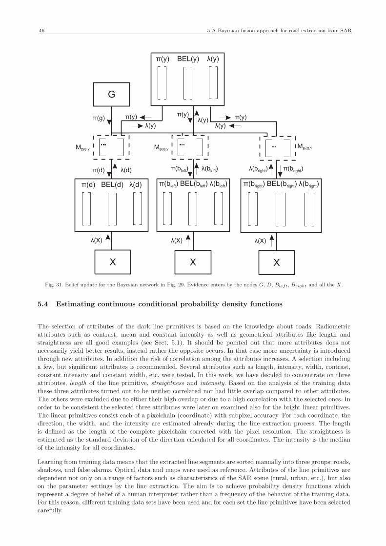
46 5 A Bayesian fusion approach for road extraction from SAR
λ( )x
λ( )bright π( )bright
MBr|G,Y
π( )y
λ( )y
π( ) λy BEL(y) (y)
G
λ( )y
π( )y
π( ) λd BEL(d) (d)
λ( )dπ( )d
MD|G,Y
...
π( )g
π( ) λb BEL(b ) (b )left left left
X
...
π( ) λb BEL(b ) (b )right right right
MBl|G,Y
...
λ( )x
X
λ( )bleftπ( )bleft
λ( )x
X
π( )yλ( )y
Fig. 31. Belief update for the Bayesian network in Fig. 29. Evidence enters by the nodes G, D, Bleft, Bright and all the X.
5.4 Estimating continuous conditional probability density functions
The selection of attributes of the dark line primitives is based on the knowledge about roads. Radiometric
attributes such as contrast, mean and constant intensity as well as geometrical attributes like length andstraightness are all good examples (see Sect. 5.1). It should be pointed out that more attributes does not
necessarily yield better results, instead rather the opposite occurs. In that case more uncertainty is introduced
through new attributes. In addition the risk of correlation among the attributes increases. A selection includinga few, but significant attributes is recommended. Several attributes such as length, intensity, width, contrast,
constant intensity and constant width, etc. were tested. In this work, we have decided to concentrate on three
attributes, length of the line primitive, straightness and intensity. Based on the analysis of the training datathese three attributes turned out to be neither correlated nor had little overlap compared to other attributes.
The others were excluded due to either their high overlap or due to a high correlation with the selected ones. In
order to be consistent the selected three attributes were later on examined also for the bright linear primitives.
The linear primitives consist each of a pixelchain (coordinate) with subpixel accuracy. For each coordinate, thedirection, the width, and the intensity are estimated already during the line extraction process. The length
is defined as the length of the complete pixelchain corrected with the pixel resolution. The straightness is
estimated as the standard deviation of the direction calculated for all coordinates. The intensity is the medianof the intensity for all coordinates.
Learning from training data means that the extracted line segments are sorted manually into three groups; roads,shadows, and false alarms. Optical data and maps were used as reference. Attributes of the line primitives are
dependent not only on a range of factors such as characteristics of the SAR scene (rural, urban, etc.), but also
on the parameter settings by the line extraction. The aim is to achieve probability density functions whichrepresent a degree of belief of a human interpreter rather than a frequency of the behavior of the training data.
For this reason, different training data sets have been used and for each set the line primitives have been selected
carefully.
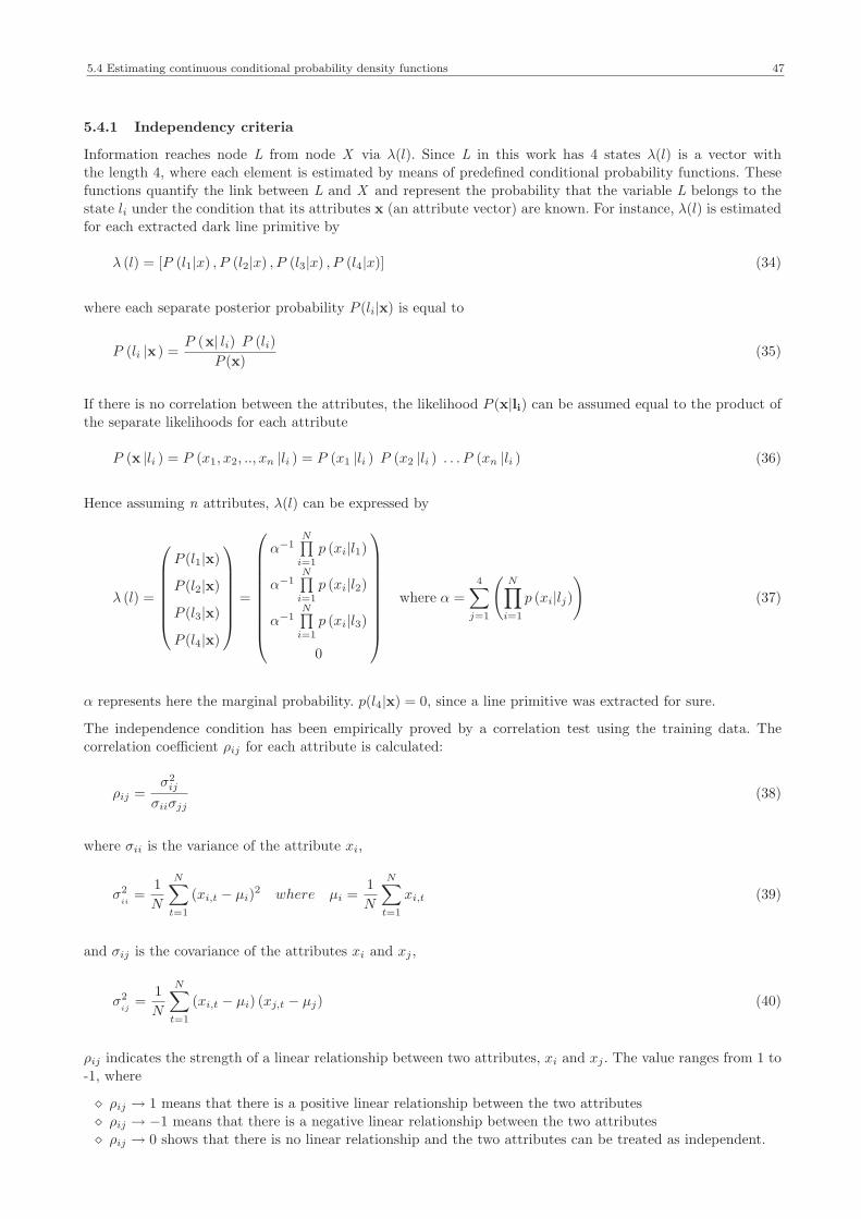
5.4 Estimating continuous conditional probability density functions 47
5.4.1 Independency criteria
Information reaches node L from node X via λ(l). Since L in this work has 4 states λ(l) is a vector with
the length 4, where each element is estimated by means of predefined conditional probability functions. These
functions quantify the link between L and X and represent the probability that the variable L belongs to thestate li under the condition that its attributes x (an attribute vector) are known. For instance, λ(l) is estimated
for each extracted dark line primitive by
λ (l) = [P (l1|x) , P (l2|x) , P (l3|x) , P (l4|x)] (34)
where each separate posterior probability P (li|x) is equal to
P (li |x ) =P (x| li) P (li)
P (x)(35)
If there is no correlation between the attributes, the likelihood P (x|li) can be assumed equal to the product of
the separate likelihoods for each attribute
P (x |li ) = P (x1, x2, .., xn |li ) = P (x1 |li ) P (x2 |li ) . . . P (xn |li ) (36)
Hence assuming n attributes, λ(l) can be expressed by
λ (l) =
P (l1|x)
P (l2|x)
P (l3|x)
P (l4|x)
=
α−1N∏
i=1
p (xi|l1)
α−1N∏
i=1
p (xi|l2)
α−1N∏
i=1
p (xi|l3)
0
where α =
4∑
j=1
(
N∏
i=1
p (xi|lj))
(37)
α represents here the marginal probability. p(l4|x) = 0, since a line primitive was extracted for sure.
The independence condition has been empirically proved by a correlation test using the training data. The
correlation coefficient ρij for each attribute is calculated:
ρij =σ2
ij
σiiσjj(38)
where σii is the variance of the attribute xi,
σ2
ii=
1
N
N∑
t=1
(xi,t − µi)2 where µi =
1
N
N∑
t=1
xi,t (39)
and σij is the covariance of the attributes xi and xj ,
σ2
ij=
1
N
N∑
t=1
(xi,t − µi) (xj,t − µj) (40)
ρij indicates the strength of a linear relationship between two attributes, xi and xj . The value ranges from 1 to
-1, where
⋄ ρij → 1 means that there is a positive linear relationship between the two attributes
⋄ ρij → −1 means that there is a negative linear relationship between the two attributes
⋄ ρij → 0 shows that there is no linear relationship and the two attributes can be treated as independent.

48 5 A Bayesian fusion approach for road extraction from SAR
Attributes of dark linear features Correlationcoefficient ρ
Attributes of dark linear features Correlationcoefficient ρ
Length - Straightness 0.0061 Straightness - Constant intensity -0.054
Length - Intensity -0.28 Straightness - Contrast -0.23
Length - Constant intensity -0.27 Intensity - Constant intensity 0.77
Length - Contrast -0.34 Intensity - Contrast 0.88
Straightness - Intensity -0.024 Constant intensity - Contrast 0.72
Tab. 4. Correlation coefficient for different attributes of dark linear features (results for the training data of roads). Strong correlationvalues are in bold.
From Tab. 4 we can draw the conclusion that only the attributes mean intensity, constant intensity and contrast
show a high correlation. This can in fact be expected due to the speckle characteristics of SAR data. As aconclusion, the factorized likelihoods can not be applied for these two attributes. The rest of the attributes did
not indicate any dependence. Fig. 32(a) exemplifies this for the two attributes length and intensity.
5.4.2 Histogram fitting
Each separate likelihood P (xi|lj) can be approximated by a probability density function learned from training
data (Hedman et al., 2006b)(Hedman et al., 2006a).
Histograms are one of the most common tools for visualizing and estimating the frequency distribution of a
data set. The Gaussian distribution
p (x| li) =1
σ√
2πe
(
− (x−µ)2
2σ2
)
(41)
is most often assumed to describe random variation that occurs in data used in most scientific disciplines.
However, if the data as in this case, shows a more skewed distribution, has a low mean value, large varianceand values cannot be negative, the distribution fits better to a log-normal distribution (Limpert et al., 2001).
Skewness of a distribution is measured by estimating the coefficient of skewness, which includes the second and
the third central moments, µ2 and µ3:
γ1 =µ3
µ3/2
2
, where µn =1
N
N∑
t=1
(xt − x)n
(42)
A random variable X is said to be log-normally distributed if log(X) is normally distributed. The rather high
skewness and remarkable high variance of the data indicated that the histograms might follow a log-normaldistribution, i.e.
p (x| li) =1
S√
2π xe−
(ln x−M)2
2S2 (43)
where M and S are the mean and standard variation of the variable’s natural logarithm. The shape of a
histogram is highly dependent on the choice of the bin size. Larger bin width normally yields histograms with a
lower resolution and as a result the shape of the underlying distribution cannot be represented correctly. Smallerbin widths produce on the other hand irregular histograms with bin heights having great statistical fluctuations.
Several formulas for finding the optimum bin width are well-known, such as Sturges’ rule or the Scott’s rule.
However most of them are based on the assumption that the data is normally distributed. Since the histogramsshow a large skewness, a method, which estimates the optimal bin size out of the data directly (Shimazaki and
Shinomoto, 2007), is used instead. Here the optimal bin width is chosen by minimizing a certain cost function,
which is estimated based on the assumption that the data in each bin obeys a Poisson distribution. The optimal
bin width is found by varying the cost function for varying bin widths (see Fig. 32(b)).
The probability density functions have been fitted to the histograms by a least square adjustment of S and
M since it allows for introducing a-priori variances (Garcia, 2000). Figs. 33, 34 and 35 show the histogram
of all attributes and their fitted log-normal distributed curve. A fitting carried out in a histogram with one
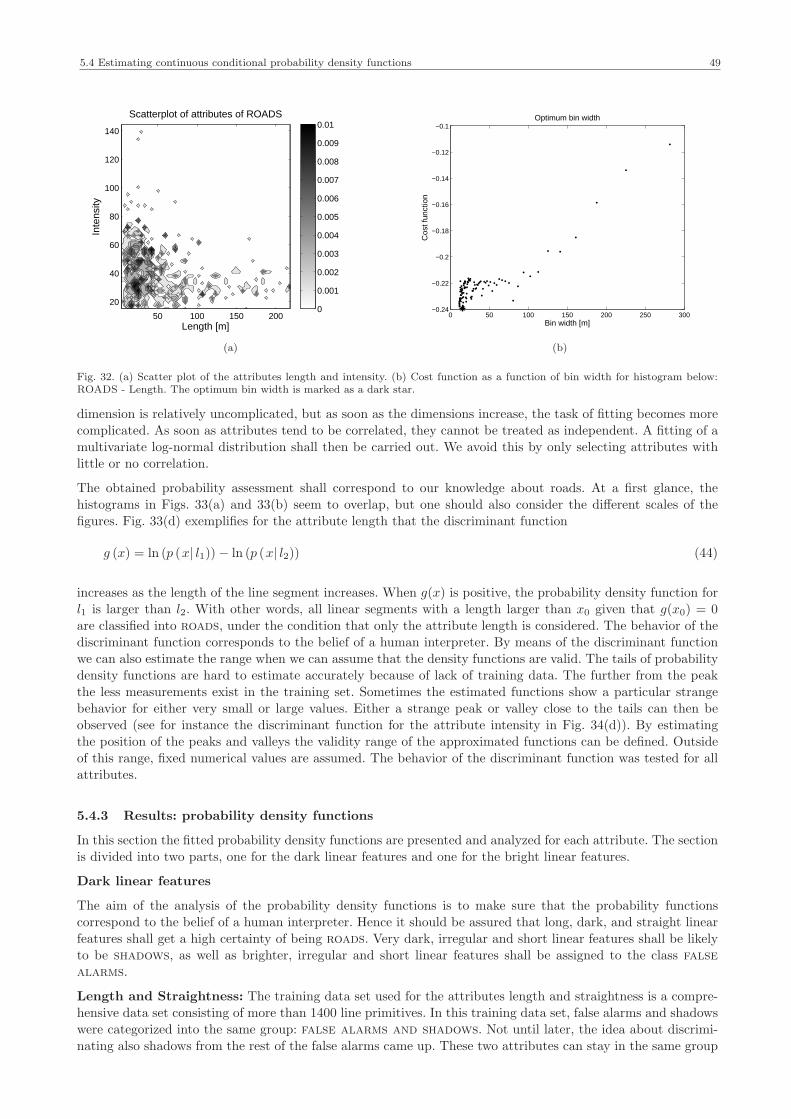
5.4 Estimating continuous conditional probability density functions 49
Length [m]
Inte
nsity
Scatterplot of attributes of ROADS
50 100 150 200
20
40
60
80
100
120
140
0
0.001
0.002
0.003
0.004
0.005
0.006
0.007
0.008
0.009
0.01
(a)
0 50 100 150 200 250 300−0.24
−0.22
−0.2
−0.18
−0.16
−0.14
−0.12
−0.1Optimum bin width
Bin width [m]
Cos
t fun
ctio
n
(b)
Fig. 32. (a) Scatter plot of the attributes length and intensity. (b) Cost function as a function of bin width for histogram below:ROADS - Length. The optimum bin width is marked as a dark star.
dimension is relatively uncomplicated, but as soon as the dimensions increase, the task of fitting becomes more
complicated. As soon as attributes tend to be correlated, they cannot be treated as independent. A fitting of amultivariate log-normal distribution shall then be carried out. We avoid this by only selecting attributes with
little or no correlation.
The obtained probability assessment shall correspond to our knowledge about roads. At a first glance, the
histograms in Figs. 33(a) and 33(b) seem to overlap, but one should also consider the different scales of the
figures. Fig. 33(d) exemplifies for the attribute length that the discriminant function
g (x) = ln (p (x| l1)) − ln (p (x| l2)) (44)
increases as the length of the line segment increases. When g(x) is positive, the probability density function for
l1 is larger than l2. With other words, all linear segments with a length larger than x0 given that g(x0) = 0are classified into roads, under the condition that only the attribute length is considered. The behavior of the
discriminant function corresponds to the belief of a human interpreter. By means of the discriminant function
we can also estimate the range when we can assume that the density functions are valid. The tails of probabilitydensity functions are hard to estimate accurately because of lack of training data. The further from the peak
the less measurements exist in the training set. Sometimes the estimated functions show a particular strange
behavior for either very small or large values. Either a strange peak or valley close to the tails can then be
observed (see for instance the discriminant function for the attribute intensity in Fig. 34(d)). By estimatingthe position of the peaks and valleys the validity range of the approximated functions can be defined. Outside
of this range, fixed numerical values are assumed. The behavior of the discriminant function was tested for all
attributes.
5.4.3 Results: probability density functions
In this section the fitted probability density functions are presented and analyzed for each attribute. The section
is divided into two parts, one for the dark linear features and one for the bright linear features.
Dark linear features
The aim of the analysis of the probability density functions is to make sure that the probability functions
correspond to the belief of a human interpreter. Hence it should be assured that long, dark, and straight linear
features shall get a high certainty of being roads. Very dark, irregular and short linear features shall be likely
to be shadows, as well as brighter, irregular and short linear features shall be assigned to the class false
alarms.
Length and Straightness: The training data set used for the attributes length and straightness is a compre-hensive data set consisting of more than 1400 line primitives. In this training data set, false alarms and shadows
were categorized into the same group: false alarms and shadows. Not until later, the idea about discrimi-
nating also shadows from the rest of the false alarms came up. These two attributes can stay in the same group

50 5 A Bayesian fusion approach for road extraction from SAR
since both of them are assumed to be irregular and short. Even though a slight majority of false alarms arerepresented in the group, the part belonging to shadows should be big enough for being statistically represented.
false alarms and shadows are in majority and represent about 4/3 (75 %) of the line primitives. The line
primitives come from different global context regions; one small part comes from forest areas (6 %), some frombuilt-up areas (37 %) and almost the half from fields (49 %). The rest were assigned to an undefined global
context - other (7 %).
The length of the line primitive is scaled by means of the pixel resolution. Straightness is defined as the
standard deviation of the orientation. Steger’s line extractor is able to define the coordinates (i.e. the points) of
the extracted line primitives with sub-pixel precision. Furthermore, for each point the width and the orientationis returned. After smoothening and re-sampling the standard deviation of the orientation for each point is
calculated.
0 200 400 600 800 1000 12000
1
2
3
4
5
6
7
8
9x 10
−3
[m]
ROADS
Training dataFitted pdf
(a)
0 50 100 150 200 250 300 3500
0.002
0.004
0.006
0.008
0.01
0.012
0.014
0.016
0.018
[m]
FALSE ALARMS and SHADOWS
(b)
0 50 100 1500
0.01
0.02
0.03
0.04
0.05
0.06
0.07
0.08
0.09
0.1
[m]
Probability density functions for length
ROADSFA and S
(c)
0 20 40 60 80 100−3
−2.5
−2
−1.5
−1
−0.5
0
0.5
[m]
Discriminant function for the attribute length
ln(p|ROADS)−ln(p|FA and S)
(d)
Fig. 33. Length: Log-normal distributions are fitted to histograms of roads (a) and false alarms and shadows (b). The approx-imated distributions for the two classes are plotted together (c). (d) The discriminant functions based on these two distributions.
Fitted probability density functions to histograms for the attributes as well as the discriminant functions forboth length and straightness can be seen in Figs 33 and 34. The estimated values for mean, variance and
skewness are listed in Tab. 5.
The plotted discriminant function for straightness shows a strange decrease close to 0 (see Fig. 34(d)). Most
probably this is due to very short line primitives with only a few pixels length. In the training data these short
line primitives are normally assigned to the class false alarms and shadows. Statistical attributes addressingdeviation and mean measures are unreliable for line primitives of only a few pixels length. Later during the
fusion procedure, very short line segments are simply sorted out. Despite of this we can make the conclusion
that line primitives belonging to a road are believed to be straighter than false alarms and shadows.

5.4 Estimating continuous conditional probability density functions 51
For this reason a threshold is defined:
p(x|ROAD) = 1
S√
2π xLe−
(ln xL−M)2
2S2 for x < xL
p(x|ROAD) = 1
S√
2π xe−
(ln x−M)2
2S2 for xL < x < 2π(45)
and
p(x|FA S) = 1
S√
2π xLe−
(ln xL−M)2
2S2 for x < xL
p(x|FA S) = 1
S√
2π xe−
(ln x−M)2
2S2 for xL < x < 2π(46)
where xL = 0.06, a local maximum obtained from the discriminant function (see Fig. 34(d)).
roads false alarms and shadows
Mean Variance Skewness Mean Variance Skewness
Length 67.8 4690 -1.88 29.4 510 -2.00
Straightness 0.257 0.0318 -3.41 0.477 0.197 -2.95
Tab. 5. Mean, variance and skewness estimated for two attributes, straightness and length.
0 0.2 0.4 0.6 0.8 1 1.2 1.4 1.60
0.5
1
1.5
2
2.5
3
3.5
4
[rad]
ROADS
Training dataFitted pdf
(a)
0 0.5 1 1.5 2 2.5 3 3.50
0.5
1
1.5
2
2.5
[rad]
FALSE ALARMS and SHADOWS
Training dataFitted pdf
(b)
0 0.5 1 1.5 20
0.5
1
1.5
2
2.5
3
3.5
4
[rad]
Probability density function for standard deviation of orientation
ROADSFA and S
(c)
0 0.5 1 1.5 2−5
−4
−3
−2
−1
0
1
2
[rad]
Discriminant function for standard deviation of orientation
ln(p(ROADS))−ln(p(FA and S))
(d)
Fig. 34. Straightness: Log-normal distributions are fitted to histograms of roads (a) and false alarms and shadows (b).The approximated distributions for the two classes are plotted together (c). (d) The discriminant functions based on these twodistributions. The star indicates the local maximum, defined as xL.
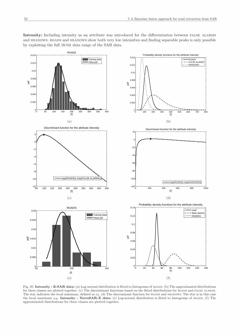
52 5 A Bayesian fusion approach for road extraction from SAR
Intensity: Including intensity as an attribute was introduced for the differentiation between false alarms
and shadows. roads and shadows show both very low intensities and finding separable peaks is only possible
by exploiting the full 16-bit data range of the SAR data.
0 50 100 150 200 250 300 350 4000
0.002
0.004
0.006
0.008
0.01
0.012
0.014
ROADS
[I]
Training dataFitted pdf
(a)
0 100 200 300 400 500 600 700 8000
0.002
0.004
0.006
0.008
0.01
0.012
0.014
[I]
Probability density functions for the attribute Intensity
ROADSFALSE ALARMSSHADOWS
(b)
50 100 150 200 250 300 350 400 450 500−12
−10
−8
−6
−4
−2
0
2
[I]
Discriminant function for the attribute intensity
ln(p(ROADS))−ln(p(FALSE ALARMS))
(c)
0 200 400 600 800 1000−120
−100
−80
−60
−40
−20
0
20
[I]
Discriminant function for the attribute intensity
ln(p(ROADS))−ln(p(SHADOWS))
(d)
50 100 1500
0.005
0.01
0.015
0.02
0.025
0.03
[I]
ROADS
Training dataFitted pdf
(e)
0 20 40 60 80 100 120 140 1600
0.02
0.04
0.06
0.08
0.1
0.12
0.14
[I]
Probability density functions for the attribute intensity
roadfalse alarmsshadows
(f)
Fig. 35. Intensity - E-SAR data: (a) Log-normal distribution is fitted to histograms of roads. (b) The approximated distributionsfor three classes are plotted together. (c) The discriminant functions based on the fitted distributions for roads and false alarms.The star indicates the local minimum, defined as xL (d) The discriminant function for roads and shadows. The star is in this casethe local maximum xH . Intensity - TerraSAR-X data: (e) Log-normal distribution is fitted to histograms of roads. (f) Theapproximated distributions for three classes are plotted together.

5.4 Estimating continuous conditional probability density functions 53
The discriminant functions seen in Figs. 35(c) and 35(d) show both strange behavior in the lower intensityregions. Irrespective of the data we can make the following conclusions:
(1) Line primitives belonging to shadows have most likely a low intensity compared to false alarms and roads.
(2) From the definition of false alarms (see Sec. 5.3) we can make the conclusion that its line primitiveshave a rather bright intensity.
Hence thresholds are defined also for the attribute intensity:
p(x|FALSE ALARM) = 0 for x < xL
p(x|FALSE ALARM) = 1
S√
2π xe−
(ln x−M)2
2S2 for x > xL
(47)
and
p(x|SHADOW ) = 1
S√
2π xe−
(ln x−M)2
2S2 for x < xH
p(x|SHADOW ) = 0 for x > xH
(48)
where xL=97.5 and xH=213 are local maximum and minimum points also obtained from the discriminant
function (see Figs. 35(c) and 35(d)). Please, note the difference between the thresholds defined here and thethresholds defined for the attribute straightness. As p(x < xL|FALSEALARMS) is equal to 0, no line primitives
with intensities below xL can be assigned to the class false alarms. At the same time, all line primitives with
an intensity higher than xH are excluded to be shadows. Whereas for straightness the probability densityfunctions are assumed to be only valid for the regions xL < x < 2π. For x < xL the likelihood probability is
assumed to be P (x|l) = P (xL|l). Otherwise very straight line primitives would be assigned to roads regardless
of its length and intensity.
Transferring the estimated probability density functions to other SAR scenes would save the user work but would
be especially difficult for the attribute intensity when different SAR sensors are used. Hence, the probability
density functions for intensity should preferably be adjusted as soon as new data sets are included. Also atraining data set from TerraSAR-X data was collected for testing the intensity range of the data. The training
data set was not as large as for the E-SAR data but large enough for the estimation of the probability density
functions (see Fig. 35(e)). While comparing the estimated functions for E-SAR data (see Fig. 35(b)) and for
TerraSAR-X data (see Fig. 35(f)) one can clearly differentiate the different intensity ranges. When the estimatedprobability density functions are applied on true data, adequate thresholds must be defined as in the case with
E-SAR data.

54 5 A Bayesian fusion approach for road extraction from SAR
Bright linear features
An E-SAR training data set showed that bright features extracted from buildings (i.e. strong scattering)are characterized by a very strong intensity and are in general short compared to the other classes. The bright
features closed to highways are usually very long, sometimes even extremely long. The intensity is low compared
to the others. At the beginning a group of false alarms (e.g. undefined bright features extracted in fields andforest) were examined. The first idea was to differentiate between straight rows of trees and other vegetation.
However these two groups showed very similar characteristics. The two classes cannot be separated based solely
on their length and intensity and it was decided to merge them into one class - vegetation. The characteristics
of Vegetation turned out to be in between highways and man-made objects in terms of both intensity andlength. The attribute straightness was excluded since the overlap was too large for all classes. There was no
strong correlation between the attributes intensity and length (see Tab. 6), except for buildings, were there seem
to be some correlation between the two attributes. This is probably due to very small but strong scatterersfrom metallic objects. The magnitude of the correlation is still less than 0.5 and the two attributes are therefore
handled as independent in this work.
Correlation between attributes: Length - In-
tensity
Highway Buildings Vegetation
Correlation coefficient ρ -0.14 -0.43 0.07
Tab. 6. Correlation coefficient estimated for the bright linear feature training set for the attribute length and intensity.
The training data set was rather small compared to the training data set of dark features and contains only115 linear features. Compared to dark linear features it was simply harder to find adequate linear primitives.
Especially the number of linear primitives belonging to the class highway was low (see Fig. 36(b)). Due to the
lack of training data the tails are especially hard to define. Therefore thresholds need to be defined for eachattribute. Within the data range defined by these thresholds, the probability density functions can be considered
reliable.
Not all functions were as skewed as those estimated for the dark features. In particular the two attributes
of highway showed a skewed distribution, which could not be described by a normal distribution. Since a
log-normal distribution is able to approach a normal distribution, log-normal distribution was assumed for allclasses.
Length:
The following assumptions were made:
(1) Bright features belonging to crash barriers of highways are usually very long, sometimes even extremelylong and are extracted with hardly any gaps.
(2) Bright features of buildings are often short. A maximum length for buildings is introduced here. However
this threshold can be adjusted according to the scene. Industrial large buildings or blocks of houses might
also cause very long bright features. Then it is more likely though that gaps occur.(3) Extracted bright vegetation features are in general not as long as highways, but longer than buildings.
The following thresholds were defined:
p(x|HIGHWAY S) = 1
S√
2π xe−
(ln x−M)2
2S2 for 0.1 < x < xH
p(x|HIGHWAY S) = 1
S√
2π xHe−
(ln xH−M)2
2S2 for x > xH
(49)
p(x|V EGETATION) = 1
S√
2π xe−
(ln x−M)2
2S2 for 0.1 < x < xH
p(x|V EGETATION) = 1
S√
2π xHe−
(ln xH−M)2
2S2 for x > xH
(50)
where xH = 87m were estimated as a local maximum in the discriminant function.
p(x|BUILDINGS) = 1
S√
2π xe−
(ln x−M)2
2S2 for x < xH
p(x|BUILDINGS) = 0 for x > xH
(51)

5.4 Estimating continuous conditional probability density functions 55
The threshold value of xH for buildings can be adjusted for each scene. It should be less than the thresholdxH for vegetation and highways. In this work we set xH equal to 50 m.
0 5 10 15 20 25 300
0.01
0.02
0.03
0.04
0.05
0.06
0.07
0.08
0.09
0.1
[m]
BUILDINGS − length
Training dataFitted pdf
(a)
300 350 400 450 500 550 6000
0.002
0.004
0.006
0.008
0.01
0.012
[I]
HIGHWAYS − intensity
Training dataFitted pdf
(b)
0 50 100 1500
0.01
0.02
0.03
0.04
0.05
0.06
0.07
0.08
0.09
0.1
[m]
Probability density functions for length
HighwaysBuildingsVegetation
(c)
0 500 1000 1500 2000 2500 3000 3500 40000
0.002
0.004
0.006
0.008
0.01
0.012Probability density functions for intensity
[I]
HighwaysBuildingsVegetation
(d)
80 100 120 140 160 180 200 2200
0.005
0.01
0.015
0.02
0.025
[I]
HIGHWAYS− Intensity
Training dataFitted pdf
(e)
0 100 200 300 400 5000
0.005
0.01
0.015
0.02
0.025
[I]
Probability density functions for intensity
HighwaysBuildingsVegetation
(f)
Fig. 36. Log-normal distributions are fitted to histograms of E-SAR training data (a) Buildings - length and (b) Highways -intensity. The resulting fitted distributions for bright linear features for three classes are plotted together; (c) length and (d)intensity. Distributions were also fitted to a small TerraSAR-X training data set. Here an example for highways is shown (e). Theestimated functions for TerraSAR-X data are plotted together (f).

56 5 A Bayesian fusion approach for road extraction from SAR
Intensity:
The probability density functions for intensity showed a good behavior for large intensities. Even going to
maximum intensities, buildings became a high assessment. Therefore we concentrated on the definition of
thresholds for the lower intensity area.
p(x|BUILDINGS) = 0 for x < xL
p(x|BUILDINGS) = 1
S√
2π xe−
(ln x−M)2
2S2 for xL < x < xH
p(x|BUILDINGS) = 1
S√
2π xHe−
(ln xH−M)2
2S2 for x > xH
(52)
where xL = 493. xH has got the same numerical value for all classes (xH = 1585).
p(x|V EGETATION) = 1
S√
2π xLe−
(ln xL−M)2
2S2 for x < xL
p(x|V EGETATION) = 1
S√
2π xe−
(ln x−M)2
2S2 for xL < x < xH
p(x|V EGETATION) = 1
S√
2π xHe−
(ln xH−M)2
2S2 for x > xH
(53)
where xL = 288 was estimated as a local minimum based on the discriminant function.
p(x|HIGHWAY ) = 1
S√
2π xLe−
(ln xL−M)2
2S2 for x < xL
p(x|HIGHWAY ) = 1
S√
2π xe−
(ln x−M)2
2S2 for xL < x < xH
p(x|HIGHWAY ) = 1
S√
2π xHe−
(ln xH−M)2
2S2 for x > xH
(54)
where the same value (xL = 288) as for vegetation was used.
As in the case with the dark linear features the intensity probability density functions should be adjusted if
they are applied to data acquired from other SAR sensors. A training data set of bright features collected
from TerraSAR-X data showed indeed that the intensities differ compared to the E-SAR data (see Figs 36(e)
and 36(f)). Hence the probability density functions should be adjusted as soon as the sensor characteristics aretoo different.
5.4.4 Evaluating and testing the classification
As soon as the training data contains a large data sample, we can use some samples for evaluating the classifi-
cation. In this work the data is randomly separated into one training set (80 % of the data) and one testing set(20 % of the data). The first set is used for the histogram fitting (i.e. building the classifier) and the second set is
used for evaluating the performance of a classifier. This classifier is nothing else than our estimated probability
density functions. The result of the evaluation is presented in a so called classification error matrix, which ispresented for each attribute. Error matrices are useful for showing the relationship between known reference
data and the correspoinding reults of the classification (Lillesand et al., 2008). The matrices are square ma-
trices with rows corresponding to the known reference and with columns with the number of the classified line
primitives. Those line primitives correctly classified can be found along the diagonal.
Producer’s accuracies are estimated from the number of correctly classified line primitives within one class
divided by the total number of line primitives of this class (the reference). It gives us an idea about how well the
testing set of one specific class is correctly classified. User’s accuracies on the other hand shows us how reliableour classification result is. This one is calculated by dividing the number of correctly classified line primitives
within each class by the total number of line primitives that were classified in that class. Overall accuracy is
calculated by dividing the number of correctly classified line primitives with the total number of line primitives.
The error matrices give information about how well the classification works for each attribute and for each class.This information is of particular importance for the design of the conditional probability table (see Sect. 5.5).
The overall accuracies for the dark linear features range from 63 % to 69 % with a better performance for the
combination of length and straightness (81 %) (see Tab. 7). The producer’s accuracies (57-83 %) and the user’s

5.4 Estimating continuous conditional probability density functions 57
accuracies (37-99 %) vary both highly between the attributes and the classes. Here there are also slightly betterresults for the combination of length and straightness (57-96 %). Normally these values give us an idea about
how well separable and homogeneous the classes are. In this case the number of false alarms dominates
the testing set that much (76 % of the first set and 72 % of the second set) that it is hard to evaluate theperformance of the two other classes.
The error matrix for the linear bright features (see Tab. 8) shows that the different bright features can be muchbetter differentiated than the dark ones. The attribute intensity alone shows an overall accuracy of 87 %. The
bright backscattering covers a large intensity range and due to the different backscattering characteristics of
the different classes, the classes can be very well distinguished. The two classes road and shadows are bothvery close in intensity range. Applying both attributes to the bright features resulted in a very good accuracy
- 96 %! However one shall keep in mind that the training data set is very small, especially the reference class
Highway. Therefore the results from the error matrix shall be handled carefully. One shall also keep in mindthat the training data was picked selective with the purpose to get homogeneous and separable classes.
One should also remember that the error matrices only give an evaluation of the classifier and not of theuncertainty assessment. The actual input to the fusion is a percentage and not an assignation to a specific class.
The uncertainty assessment is also a result of the product of all probabilities (Eq. 36).
Error Matrix: Dark Features
Length
R FA and S Total User’s Accuracy Producer’s Accuracy Overall Accuracy
r 47 70 117 0.40 0.66
fa and s 24 145 169 0.86 0.67
Total 71 215 286 0.67
Straightness
R FA and S Total User’s Accuracy Producer’s Accuracy Overall Accuracy
r 59 93 152 0.39 0.83
fa and s 12 122 134 0.91 0.57
Total 71 215 286 0.63
Intensity - E-SAR data
R FA S Total User’s Accuracy Producer’s Accuracy Overall Accuracy
r 41 59 11 111 0.37 0.71
fa 1 156 0 157 0.99 0.69
s 16 11 17 44 0.39 0.61
Total 58 226 28 312 0.69
Length, Straightness, Intensity
R FA S Total User’s Accuracy Producer’s Accuracy Overall Accuracy
r 39 24 9 72 0.54 0.67
fa 9 187 2 198 0.94 0.83
s 10 15 17 42 0.40 0.61
Total 58 226 28 312 0.78
Tab. 7. Error matrix for the attributes; length, straightness and intensity. Capital letters indicate the reference and the classificationresults are referred to as the lowercase letters (such as R=reference for ROADS, r=classified line primitives into the class ROAD).
In order to get an idea of how the classifier works it was also tested on a line extraction from real data. The lineextraction is carried out with a different parameter setting compared to the training data. The small sub-images
come from the same scene as the training data, but the training data was collected from different parts. A visual
inspection of the results implies that the classification delivers overall good results. Especially open roads (seeFig. 37) and highways (see Fig. 38) are in most cases correctly classified. Here the line extraction is successful.
The extracted line primitives are usually long and straight. The classification also works well for most of the
false alarms extracted in fields (see Fig. 37) and forest areas, as well as for very dark irregular shadow regions
(see Fig. 38).
There are certain problematic areas where it is hard to achieve a reliable classification. Built-up areas is in
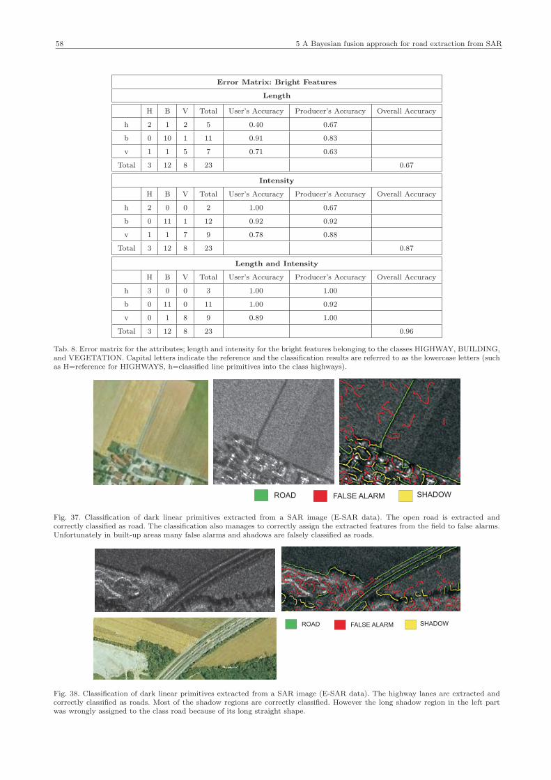
58 5 A Bayesian fusion approach for road extraction from SAR
Error Matrix: Bright Features
Length
H B V Total User’s Accuracy Producer’s Accuracy Overall Accuracy
h 2 1 2 5 0.40 0.67
b 0 10 1 11 0.91 0.83
v 1 1 5 7 0.71 0.63
Total 3 12 8 23 0.67
Intensity
H B V Total User’s Accuracy Producer’s Accuracy Overall Accuracy
h 2 0 0 2 1.00 0.67
b 0 11 1 12 0.92 0.92
v 1 1 7 9 0.78 0.88
Total 3 12 8 23 0.87
Length and Intensity
H B V Total User’s Accuracy Producer’s Accuracy Overall Accuracy
h 3 0 0 3 1.00 1.00
b 0 11 0 11 1.00 0.92
v 0 1 8 9 0.89 1.00
Total 3 12 8 23 0.96
Tab. 8. Error matrix for the attributes; length and intensity for the bright features belonging to the classes HIGHWAY, BUILDING,and VEGETATION. Capital letters indicate the reference and the classification results are referred to as the lowercase letters (suchas H=reference for HIGHWAYS, h=classified line primitives into the class highways).
ROAD FALSE ALARM SHADOW
Fig. 37. Classification of dark linear primitives extracted from a SAR image (E-SAR data). The open road is extracted andcorrectly classified as road. The classification also manages to correctly assign the extracted features from the field to false alarms.Unfortunately in built-up areas many false alarms and shadows are falsely classified as roads.
ROAD FALSE ALARM SHADOW
Fig. 38. Classification of dark linear primitives extracted from a SAR image (E-SAR data). The highway lanes are extracted andcorrectly classified as roads. Most of the shadow regions are correctly classified. However the long shadow region in the left partwas wrongly assigned to the class road because of its long straight shape.
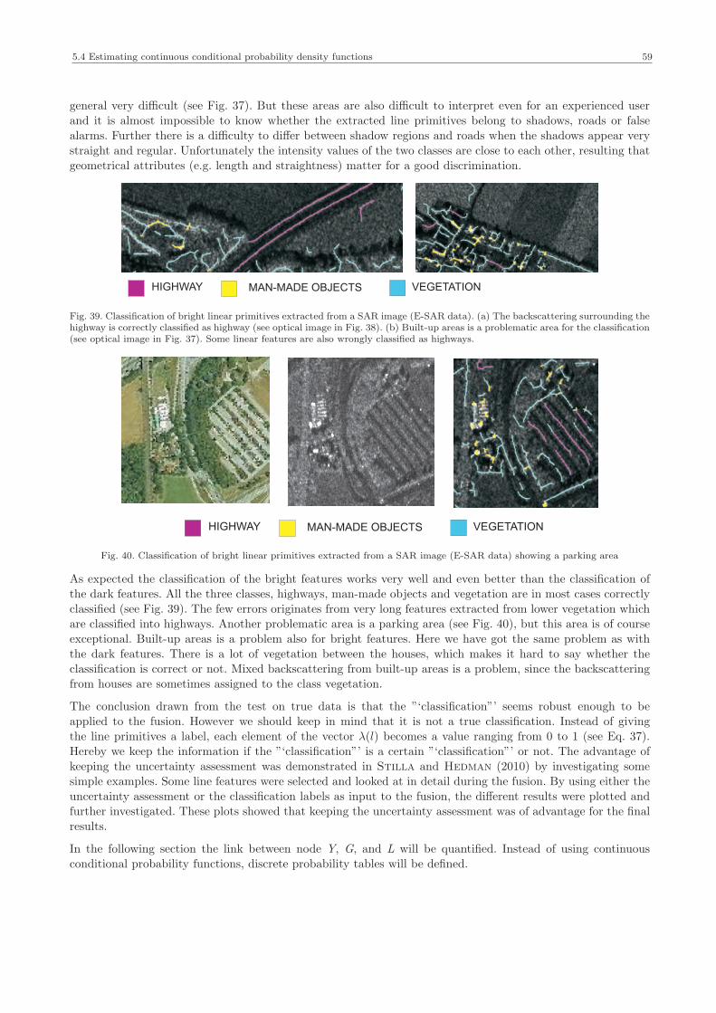
5.4 Estimating continuous conditional probability density functions 59
general very difficult (see Fig. 37). But these areas are also difficult to interpret even for an experienced userand it is almost impossible to know whether the extracted line primitives belong to shadows, roads or false
alarms. Further there is a difficulty to differ between shadow regions and roads when the shadows appear very
straight and regular. Unfortunately the intensity values of the two classes are close to each other, resulting thatgeometrical attributes (e.g. length and straightness) matter for a good discrimination.
HIGHWAY MAN-MADE OBJECTS VEGETATION
Fig. 39. Classification of bright linear primitives extracted from a SAR image (E-SAR data). (a) The backscattering surrounding thehighway is correctly classified as highway (see optical image in Fig. 38). (b) Built-up areas is a problematic area for the classification(see optical image in Fig. 37). Some linear features are also wrongly classified as highways.
HIGHWAY MAN-MADE OBJECTS VEGETATION
Fig. 40. Classification of bright linear primitives extracted from a SAR image (E-SAR data) showing a parking area
As expected the classification of the bright features works very well and even better than the classification ofthe dark features. All the three classes, highways, man-made objects and vegetation are in most cases correctly
classified (see Fig. 39). The few errors originates from very long features extracted from lower vegetation which
are classified into highways. Another problematic area is a parking area (see Fig. 40), but this area is of courseexceptional. Built-up areas is a problem also for bright features. Here we have got the same problem as with
the dark features. There is a lot of vegetation between the houses, which makes it hard to say whether the
classification is correct or not. Mixed backscattering from built-up areas is a problem, since the backscatteringfrom houses are sometimes assigned to the class vegetation.
The conclusion drawn from the test on true data is that the ”‘classification”’ seems robust enough to be
applied to the fusion. However we should keep in mind that it is not a true classification. Instead of givingthe line primitives a label, each element of the vector λ(l) becomes a value ranging from 0 to 1 (see Eq. 37).
Hereby we keep the information if the ”‘classification”’ is a certain ”‘classification”’ or not. The advantage of
keeping the uncertainty assessment was demonstrated in Stilla and Hedman (2010) by investigating some
simple examples. Some line features were selected and looked at in detail during the fusion. By using either theuncertainty assessment or the classification labels as input to the fusion, the different results were plotted and
further investigated. These plots showed that keeping the uncertainty assessment was of advantage for the final
results.
In the following section the link between node Y, G, and L will be quantified. Instead of using continuous
conditional probability functions, discrete probability tables will be defined.

60 5 A Bayesian fusion approach for road extraction from SAR
5.5 Conditional probability tables
While the conditional probability functions defined in the previous section (see Sect. 5.4) quantify the link
between the detected line primitive L and their attributes X, the conditional probability table defined in this
section shall express the relation between the existing object, Y, and the extracted line primitives, L. Since wemove in the same direction as the arrow (i.e. from causes to effects) the conditional probability table should
quantify the probability that a certain object in the scene should give rise to detected line features. During the
process of defining the conditional probability table three points must be taken into consideration;
(1) the road model considering different sensor geometries (Sect. 5.1.1),(2) the performance of the line extractor (Sect. 5.2.1)
(3) the performance of the probability density functions - our ”classifier” (Sect. 5.4)
5.5.1 Definition of conditional probability table - without local context
The capacity of estimating conditional probability density functions is dependent on the availability of trainingdata. If one has no access to sufficient training data, one is forced to express the belief by tables consisting of
discrete probabilities. At best, probabilities can be numerically estimated directly from training data. In the
worst case they have to be estimated based on subjective belief. In this work most numerical values representingthe conditional probabilities originates from the previous analysis of training data and the model of road and
its local context. But due to lack of training data some conditional probabilities needed to be estimated based
on a subjective belief.
We will start with the Bayesian network (s. Eq. 26) which do not include the bright features. The conditional
probability table, ML|Y,G should quantify the arrows Y → L and G → L. If the two parental nodes were assumedto have independent causation on L the arrows could be treated individually. However the two parental nodes
have a strong correlated influence on L meaning that the conditional probability table (P (l|y, g)) needs to be
defined for both variables. This means that every combination of conditions that might cause L must be stored.As stated in Sect. 5.3, Y and G are d-connected as soon as evidence will enter variable L.
Each column of ML|Yishall comprise the following two questions:
⋄ “What is the probability that a possible object Yi illuminated with a certain sensor geometry will be detected
by the line extractor?”
⋄ “... and if detected, what is the probability that the line primitive is assigned to the state li?’
Hence the node L also comprises the information if a line extraction succeeded or not. We assume that e1
represent that a line feature was extracted and e2 that nothing was detected. The probability that the line
extraction will be successful can be as in earlier work be estimated based on subjective belief (Hedman et al.,
2007)(Hedman et al., 2008), but estimating numerical values based on training data is a better option. Inthis work the probability of detecting a line primitive with the characteristics of being a road P (e1|y1) = 0.87
if the road is visible is given by the completeness values of the line extractor (see Tab. 3). Next we should
find P (l1, e1|y1, gk) which is the answer to the second question above. The product rule allows the following
expression:
p(li, e1|yj , gk) = p(li|e1, yj , gk) p(e1|yj , gk) (55)
where p(li|e1, yj , gk) can be estimated based on the error matrix (see Tab. 7) assuming that all objects yi werevisible during the SAR acquisition. The error matrix gives us information about the performance of the classifier.
Producer’s accuracies tell us the probability that a line feature is correctly assigned to a class. Indeed some line
primitives of the reference class road are falsely classified. Furthermore the error matrix gives us the usefulinformation that a road is more likely to be falsely classified as a shadow as a false alarm.
Since e2 is equal to the state L = l4 we can simply write P (l4, e2|yj , gk) as P (l4|yj , gk). The notation p(li|yj , gk)
is used for simplicity in the following text but is in reality equal to p(li, e|yj , gk).
Assessing the numerical values for p(li|yj , gk) for each state yj is more complicated for those objects Y which
are influenced by the sensor geometry. We need to answer on the question when we can expect to see ourroad in the SAR image. And if the road cannot be seen, what do we expect then? Fig. 41 shows how the
object Y and the sensor geometry G are likely to cause different states of L. Here one can see that the node
G is quantified through the width of an assumed shadow SN . Certainly G can enter all kind of states gk but

5.5 Conditional probability tables 61
there is not a chance that we can collect training data enough for covering the range of SN . Most difficult isthe estimation of p(e1|yj , gk) for some states of Y. For instance no reference data could be defined for clutter,
meaning that p(e1|clutter had to be defined by the user. In this work we call these manually defined assumptions
subjective probabilities. In addition the line extractor is restricted by the width, meaning that p(e1|yj , gk) canvary dependent on the object Y. This would be straight forward to estimate numerically if the height of the
object was either known before or estimated during the fusion. Since the height of high objects is set by the user
the definition of p(e1|yj , gk) should not be too severe since a false estimation of the height must be included aswell.
Linear shape, typicalcharacteristics of a
road (L=l )1
All sensor geometries
OPEN ROADROAD AND VEGETATIONTOWARDS THE SENSOR
Linear shape, typicalcharacteristics of a
road
Linearshadowregion
Road still visible Shadow occludes road
Wide shadowdetect
W <S <WR N NoL S >WN NoL
HIGH OBJECT(building or trees)
Linear shadow region(L=l )3
Shadow
W <S <WMin N NoL S >WN NoLS <WN RS <WN Min
Nothing ora falsealarm
Node Y:
Node G:
Node L:
Wide shadow(L=l ) or a
false alarm4
Fig. 41. The relation between roads, local context, sensor geometries and the appearance in the SAR image, which is the underlyingmodel behind the Bayesian network.
Open roads (y1): The sensor geometry has no influence on the appearance of the road. There are no localcontext that might influence the appearance of the road in the SAR image. The road shall show the same
characteristics, no matter from what direction the SAR image is acquired.
Roads with high objects nearby (y2): As discussed in Sect. 5.1.2, the road with trees or houses nearby showdifferent characteristics in the SAR scene depending on the β angle. Based on Fig. 15 following assumptions
can be made:
(1) Sn < WR: The shadow occludes only a part of the road and the typical road characteristics are supposed
to be kept.
(2) WR < Sn < WNoL: The shadow occludes the whole road. A line extraction is still possible and an
extracted line primitive will have the same characteristics as an extracted shadow region.(3) Sn > WNoL: Range is almost perpendicular to the direction of the road. The width of the shadow is
assumed to be too large for the line extraction.
The conclusion drawn from these statements is that depending on the sensor geometry different states of L are
expected. For each state gk not only each p(li|y2, gk) is different, but also p(e1|y2, gk) must vary. When the road
is assumed to be visible (Sn < WR) the same chances of a line extraction and characteristics as an open road is
assumed. Hence the column p(l|y1) is equal to p(l|y2). As we continue to the next domain, WR < Sn < WNoL,a shadow is expected. The column should therefore express the performance of the line extractor for detecting
shadow regions as well as the performance of the classifier. For the domain Sn > WNoL the numerical estimates
are much harder. The following subjective probabilities are assumed:
⋄ There is a 50% chance that the line extractor will work anyway.
⋄ Among these detected 50%, 25%of these will have the same characteristics as false alarms
High Objects
(1) Sn < WMinL: Either no shadow is present or the linear shadow region is supposed to be too thin for theline extractor. If something is extracted it is assumed to be only clutter.
(2) WMinL < Sn < WNoL: A line extraction is possible and the extracted line primitive will have the typical
characteristics of an extracted shadow region.
(3) Sn > WNoL: Range is almost perpendicular to the high object. The width of the shadow is assumed tobe too large for the line extraction.
For the domain Sn < WMinL nothing or a false alarm is expected. It is assumed that a width larger than WMinL
is needed for a line extraction to succeed. The reasoning behind the definition of p(l|y4) can be found under
”‘Clutter”’. The definition of p(l|y3) for the domain WMinL < Sn < WNoL is based on the same calculations
as for roads with objects nearby (WR < Sn < WNoL) resulting in p(l|y3) = p(l|y2). That is also valid for
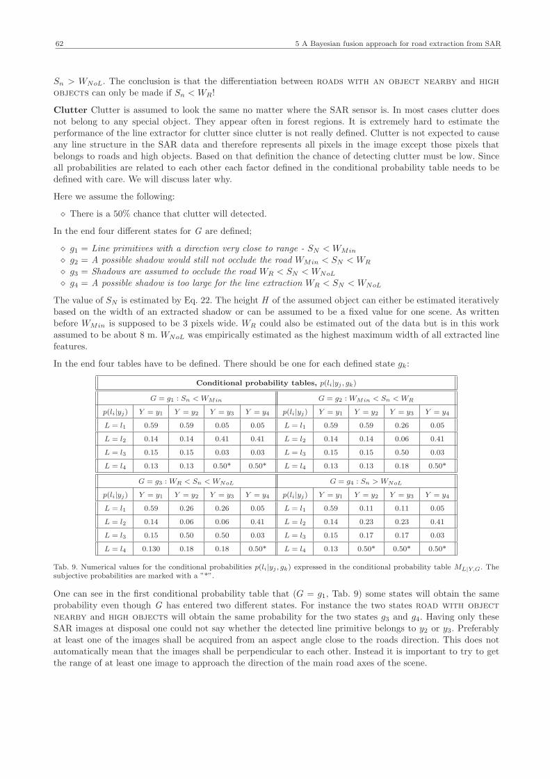
62 5 A Bayesian fusion approach for road extraction from SAR
Sn > WNoL. The conclusion is that the differentiation between roads with an object nearby and high
objects can only be made if Sn < WR!
Clutter Clutter is assumed to look the same no matter where the SAR sensor is. In most cases clutter does
not belong to any special object. They appear often in forest regions. It is extremely hard to estimate theperformance of the line extractor for clutter since clutter is not really defined. Clutter is not expected to cause
any line structure in the SAR data and therefore represents all pixels in the image except those pixels that
belongs to roads and high objects. Based on that definition the chance of detecting clutter must be low. Sinceall probabilities are related to each other each factor defined in the conditional probability table needs to be
defined with care. We will discuss later why.
Here we assume the following:
⋄ There is a 50% chance that clutter will detected.
In the end four different states for G are defined;
⋄ g1 = Line primitives with a direction very close to range - SN < WMin
⋄ g2 = A possible shadow would still not occlude the road WMin < SN < WR
⋄ g3 = Shadows are assumed to occlude the road WR < SN < WNoL
⋄ g4 = A possible shadow is too large for the line extraction WR < SN < WNoL
The value of SN is estimated by Eq. 22. The height H of the assumed object can either be estimated iteratively
based on the width of an extracted shadow or can be assumed to be a fixed value for one scene. As writtenbefore WMin is supposed to be 3 pixels wide. WR could also be estimated out of the data but is in this work
assumed to be about 8 m. WNoL was empirically estimated as the highest maximum width of all extracted line
features.
In the end four tables have to be defined. There should be one for each defined state gk:
Conditional probability tables, p(li|yj , gk)
G = g1 : Sn < WMin G = g2 : WMin < Sn < WR
p(li|yj) Y = y1 Y = y2 Y = y3 Y = y4 p(li|yj) Y = y1 Y = y2 Y = y3 Y = y4
L = l1 0.59 0.59 0.05 0.05 L = l1 0.59 0.59 0.26 0.05
L = l2 0.14 0.14 0.41 0.41 L = l2 0.14 0.14 0.06 0.41
L = l3 0.15 0.15 0.03 0.03 L = l3 0.15 0.15 0.50 0.03
L = l4 0.13 0.13 0.50* 0.50* L = l4 0.13 0.13 0.18 0.50*
G = g3 : WR < Sn < WNoL G = g4 : Sn > WNoL
p(li|yj) Y = y1 Y = y2 Y = y3 Y = y4 p(li|yj) Y = y1 Y = y2 Y = y3 Y = y4
L = l1 0.59 0.26 0.26 0.05 L = l1 0.59 0.11 0.11 0.05
L = l2 0.14 0.06 0.06 0.41 L = l2 0.14 0.23 0.23 0.41
L = l3 0.15 0.50 0.50 0.03 L = l3 0.15 0.17 0.17 0.03
L = l4 0.130 0.18 0.18 0.50* L = l4 0.13 0.50* 0.50* 0.50*
Tab. 9. Numerical values for the conditional probabilities p(li|yj , gk) expressed in the conditional probability table ML|Y,G. Thesubjective probabilities are marked with a ”*”.
One can see in the first conditional probability table that (G = g1, Tab. 9) some states will obtain the same
probability even though G has entered two different states. For instance the two states road with object
nearby and high objects will obtain the same probability for the two states g3 and g4. Having only theseSAR images at disposal one could not say whether the detected line primitive belongs to y2 or y3. Preferably
at least one of the images shall be acquired from an aspect angle close to the roads direction. This does not
automatically mean that the images shall be perpendicular to each other. Instead it is important to try to get
the range of at least one image to approach the direction of the main road axes of the scene.

5.5 Conditional probability tables 63
5.5.2 Definition of conditional probability table - including local context
A conditional probability table for a fusion that includes the bright feature extraction must also take the
performance of the bright line extractor, the performance of “the bright classifier” and the relation between theobject, the sensor geometry and the extracted dark and bright features in consideration.
The conditional tables that needs to be defined are far more complex than the previous one. Since there arethree nodes,D, Bleft and Bright, three tables are constructed. In addition the node G is no longer quantified
by only Sn, but also the length of layover, LN . In addition the bright features are on the side which faces or is
opposite to the sensor plays a certain role. Hence the number of states of G is further increased. If we would
design the conditional probability table in the same way as in the previous section (Sect. 5.5.2) we would endup with an endless number of states and several conditional probability tables.
The difficulty lies in the modeling. It is hard to find a model which on one side is detailed enough for includingthe characteristics for each object. On the other side the model should not be too detailed in oder to avoid
over-fitting.
The three classes open road, highway and clutter have all in common that these are independent on the sensor
geometry. No matter the sensor geometry, the performance of the line extractor and the classifier stay the same.
Next to open roads we do not expect to find any local context. If a bright feature is extracted then it can beassumed to be only bright clutter. Next to highways we can expect to find bright extracted feature classified as
highways. These are assumed to be well detectable no matter the sensor geometry. Also these are expected to
be extracted on both sides of the road. Clutter is assumed to consist of dark and bright false alarms only.
D
Y G
CD CBL CBR
XDXBl XBr
Bleft Bright
(a)
λ( )d
λ( )c π( )c
MC|G,Y
π( )gπ( )y
λ( )y
C
...
MD|C
...
π( )d
MD|G,Y
(b)
Fig. 42. (a) The hidden nodes CD, CBL, and CBR are inserted in the Bayesian network BN4. (b) The belief update including thehidden node C is illustrated. MC|Y,G and MD|C create together MD|Y,G.
As soon as local context represents high objects such as high trees or high buildings, the sensor geometry has
a strong impact on what the local context and the road (if existing) look like in the SAR image. For instanceif a row of trees exists next to the road, the sensor geometry is the critical factor for the possibility to extract
a linear dark feature and if this extracted linear feature belongs to a road or a shadow. Furthermore the sensor
geometry influences the possibility that the bright line extractor detects the row of trees. Common for the classesy3 − y9 (see definition in Sect 5.3) is that all classes comprise high objects meaning that the sensor geometry
needs to be incorporated in the definition of the conditional probability tables. In previous section we could not
differentiate whether the local context was on the left or on the right side of the road. The assumed shadow was
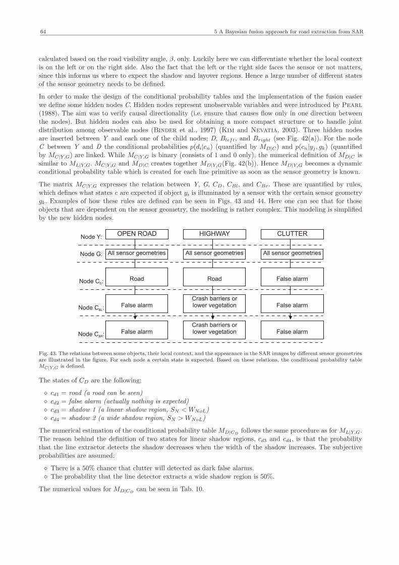
64 5 A Bayesian fusion approach for road extraction from SAR
calculated based on the road visibility angle, β, only. Luckily here we can differentiate whether the local contextis on the left or on the right side. Also the fact that the left or the right side faces the sensor or not matters,
since this informs us where to expect the shadow and layover regions. Hence a large number of different states
of the sensor geometry needs to be defined.
In order to make the design of the conditional probability tables and the implementation of the fusion easier
we define some hidden nodes C. Hidden nodes represent unobservable variables and were introduced by Pearl
(1988). The aim was to verify causal directionality (i.e. ensure that causes flow only in one direction betweenthe nodes). But hidden nodes can also be used for obtaining a more compact structure or to handle joint
distribution among observable nodes (Binder et al., 1997) (Kim and Nevatia, 2003). Three hidden nodes
are inserted between Y and each one of the child nodes; D, Bleft, and Bright (see Fig. 42(a)). For the nodeC between Y and D the conditional probabilities p(di|cn) (quantified by MD|C) and p(cn|yj , gk) (quantified
by MC|Y,G) are linked. While MC|Y,G is binary (consists of 1 and 0 only), the numerical definition of MD|C is
similar to ML|Y,G. MC|Y,G and MD|C creates together MD|Y,G(Fig. 42(b)). Hence MD|Y,G becomes a dynamic
conditional probability table which is created for each line primitive as soon as the sensor geometry is known.
The matrix MC|Y,G expresses the relation between Y, G, CD, CBl, and CBr. These are quantified by rules,
which defines what states c are expected if object yi is illuminated by a sensor with the certain sensor geometrygk. Examples of how these rules are defined can be seen in Figs. 43 and 44. Here one can see that for those
objects that are dependent on the sensor geometry, the modeling is rather complex. This modeling is simplified
by the new hidden nodes.
Road
All sensor geometries
OPEN ROAD
Node C :D
False alarmNode :CBL
False alarmNode :CBR
Road
All sensor geometries
HIGHWAY
Crash barriers orlower vegetation
Crash barriers orlower vegetation
False alarm
All sensor geometries
CLUTTER
False alarm
False alarm
Node G:
Node Y:
Fig. 43. The relations between some objects, their local context, and the appearance in the SAR images by different sensor geometriesare illustrated in the figure. For each node a certain state is expected. Based on these relations, the conditional probability tableMC|Y,G is defined.
The states of CD are the following;
⋄ cd1 = road (a road can be seen)
⋄ cd2 = false alarm (actually nothing is expected)
⋄ cd3 = shadow 1 (a linear shadow region, SN < WNoL)⋄ cd4 = shadow 2 (a wide shadow region, SN > WNoL)
The numerical estimation of the conditional probability table MD|CDfollows the same procedure as for ML|Y,G.
The reason behind the definition of two states for linear shadow regions, cd3 and cd4, is that the probabilitythat the line extractor detects the shadow decreases when the width of the shadow increases. The subjective
probabilities are assumed:
⋄ There is a 50% chance that clutter will detected as dark false alarms.⋄ The probability that the line detector extracts a wide shadow region is 50%.
The numerical values for MD|CDcan be seen in Tab. 10.

5.5 Conditional probability tables 65
W <S <WR N NoLL <(W -W )N R min
Road False alarm
Vegetation is on the side which facesthe sensor
Node :CD
Node :CBL
Node G:
Node Y:
Node G:
Vegetation is on the side which isopposite to the sensor
W <S <WR N NoL S >WN NoLS <WN R
Road Shadow1 Shadow2
L <N WMinL >N WMin
Vegetation2
Node :CBR
Vegetation2
False alarm False alarm
Vegetation is on the leftside of the road
L <N WMinL >N WMin
Vegetation2 Vegetation1
False alarm False alarm
Node :CBL
Node Y:
Node G:
Right side faces the sensor
(W -L -S )<WR N N min
Shadow1Node :CD
Node G:( )>W -L -S WR N N min
Road
Node :CBR
Left side faces the sensor
L <N WMinL >N WMin
Vegetation2 Vegetation2
Vegetation2 Vegetation1
Vegetation is onboth sides of the road
L <N WMinL >N WMin
Vegetation2 Vegetation1
Vegetation2 Vegetation2
False alarm
Vegetation is on the side which facesthe sensor
Node :CD
Node :CBL
Node G:
Node Y:
Node G:
Vegetation is on the side which isopposite to the sensor
W <S <Wmin N NoL S >WN NoLS <N Wmin
False alarm Shadow1 Shadow2
L <N WMinL >N WMin
Vegetation2
Node :CBR
Vegetation2
False alarm False alarm
Vegetation only - the vegetation is onthe left side of a detected dark feature
L <N WMinL >N WMin
Vegetation2 Vegetation1
False alarm False alarm
Fig. 44. The relations between some objects, their local context, and the appearance in the SAR image by different sensor geometriesare shown in the figure. The appearance for all objects is strongly dependent on the sensor geometry. For each node a certain stateis expected. Based on these relations, the conditional probability table MC|Y,G is defined.

66 5 A Bayesian fusion approach for road extraction from SAR
The states defined for CBr and CBl are:
⋄ cb1 = the borders of the highway (crash barriers or low vegetation)⋄ cb2 = vegetation 1 (a layover region can clearly be seen)
⋄ cb3 = vegetation 2 - no layover
⋄ cb4 = scattering from buildings/man-made objects - with layover⋄ cb5 = scattering from buildings/man-made objects - no layover
⋄ cb6 = false alarm (nothing is expected)
The definition of MCBr|Y,Gis carried out slightly different compared to MD|CD
The number of samples for the
evaluation of the bright linear classification (Sect. 5.4.4) was unfortunately small. Instead of estimating the
performance for each individual class, the overall performance was estimated. According to Tab. 8 the classifiermanaged to classify 96% of the bright features correctly. The numerical values for the performance of the line
extractor for the individual classes were taken from Tab. 3.
Two states for vegetation and buildings/man-made objects are defined. The reason for this is that vegetation
and building are more likely to be detected when layover occur. The following assumption was made:
⋄ The probability that the line detector extracts vegetation or a building even though no layover occurs is50%.
Bright clutter needs to be modeled just as all the other bright feature classes. Here the same problem as with
the definition of dark clutter turns up. How can we estimate the performance of detecting clutter since we have
no training data? As stated in the analysis of the performance of the line extractor (see Sect. 5.2.1) there is a
tendency to more over-segmentation in terms of dark than in terms of bright features. We can therefore assumethat less bright clutter is detected. If bright clutter is detected it has the characteristics of bright false alarms.
Since bright false alarms were not included in the classifier the probability that the classifier is assigned to a
particular class is supposed to be the same for all classes.
⋄ There is a 25% chance that bright clutter will be detected.⋄ If bright clutter is detected, it has the appearance of a bright false alarm.
⋄ The probability that the false alarm is classified into one of the three class: 100/3 = 33 %
The numerical values for MBl=Br|CBcan be seen in Tab. 11.
Conditional Probabilities for Dark Features
p(di|cj) C = Cd1 C = Cd2 C = Cd3 C = Cd4
D = d1 0.59 0.05 0.26 0.16
D = d2 0.14 0.41 0.06 0.04
D = d3 0.15 0.03 0.50 0.30
D = d4 0.13 0.50* 0.18 0.50*
Tab. 10. Numerical values for the conditional probabilities p(di|cj). The table quantifies the link between node D and the hiddennode CD. The subjective probabilities are marked with a ”*”.
Conditional Probabilities for Bright Features
p(bi|cj) C = Cb1 C = Cb2 C = Cb3 C = Cb4 C = Cb5 C = Cb6
B = b1 0.77 0.02 0.01 0.02 0.01 0.08*
B = b2 0.02 0.02 0.01 0.88 0.48 0.08*
B = b3 0.02 0.90 0.48 0.02 0.01 0.08*
B = b4 0.20 0.06 0.50* 0.08 0.50* 0.75*
Tab. 11. Numerical values for the conditional probabilities p(bi|cj). The table quantifies the link between node D and the hiddennodes CBL and CBR. The subjective probabilities are marked with a ”*”.
The binary table MC|Y,G needs to consider a large number of states for G, which are all dependent on:
⋄ The assumed shadow length SN can be within the ranges SN < WMin, SN < WR, WR < SN < WNoL, and
SN > WNoL.
⋄ The assumed layover length LN can be within the ranges LN < WMin and LN > WMin.

5.5 Conditional probability tables 67
⋄ The lengths of both layover and shadow might be within (WR −LN −SN ) > WMin and (WR −LN −SN ) <
WMin
⋄ ”‘The left side of the detected dark linear primitive D faces the sensor”’ or ”‘The right side of the detected
dark linear primitive D faces the sensor”’
Instead of setting up such a table by the implementation, certain rules for each object are set up. The rules are
defined as illustrated in Figs. 43 and 44. Buildings are treated the same as the object ”‘vegetation only”’.
At this stage all conditional probabilities among the nodes are learned. The complete learning is fulfilled as the
prior term is also defined. That will be discussed in the following section.
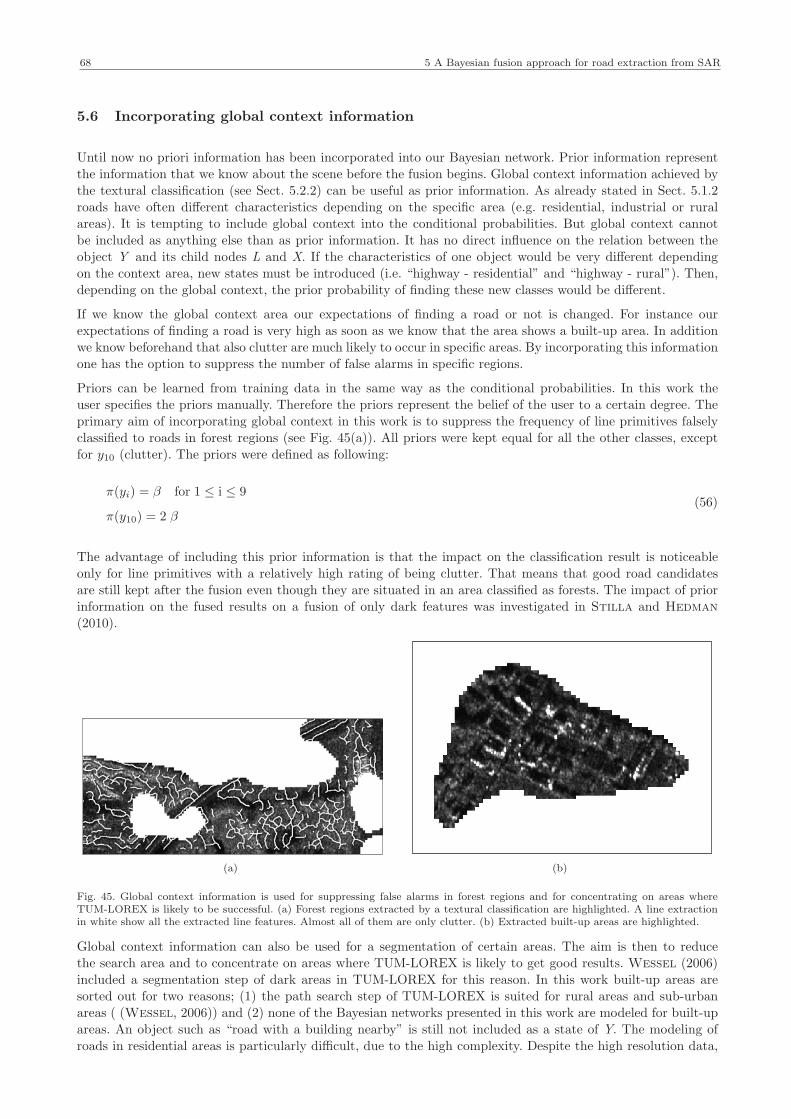
68 5 A Bayesian fusion approach for road extraction from SAR
5.6 Incorporating global context information
Until now no priori information has been incorporated into our Bayesian network. Prior information represent
the information that we know about the scene before the fusion begins. Global context information achieved by
the textural classification (see Sect. 5.2.2) can be useful as prior information. As already stated in Sect. 5.1.2roads have often different characteristics depending on the specific area (e.g. residential, industrial or rural
areas). It is tempting to include global context into the conditional probabilities. But global context cannot
be included as anything else than as prior information. It has no direct influence on the relation between theobject Y and its child nodes L and X. If the characteristics of one object would be very different depending
on the context area, new states must be introduced (i.e. “highway - residential” and “highway - rural”). Then,
depending on the global context, the prior probability of finding these new classes would be different.
If we know the global context area our expectations of finding a road or not is changed. For instance ourexpectations of finding a road is very high as soon as we know that the area shows a built-up area. In addition
we know beforehand that also clutter are much likely to occur in specific areas. By incorporating this information
one has the option to suppress the number of false alarms in specific regions.
Priors can be learned from training data in the same way as the conditional probabilities. In this work theuser specifies the priors manually. Therefore the priors represent the belief of the user to a certain degree. The
primary aim of incorporating global context in this work is to suppress the frequency of line primitives falsely
classified to roads in forest regions (see Fig. 45(a)). All priors were kept equal for all the other classes, exceptfor y10 (clutter). The priors were defined as following:
π(yi) = β for 1 ≤ i ≤ 9
π(y10) = 2 β(56)
The advantage of including this prior information is that the impact on the classification result is noticeable
only for line primitives with a relatively high rating of being clutter. That means that good road candidates
are still kept after the fusion even though they are situated in an area classified as forests. The impact of priorinformation on the fused results on a fusion of only dark features was investigated in Stilla and Hedman
(2010).
(a) (b)
Fig. 45. Global context information is used for suppressing false alarms in forest regions and for concentrating on areas whereTUM-LOREX is likely to be successful. (a) Forest regions extracted by a textural classification are highlighted. A line extractionin white show all the extracted line features. Almost all of them are only clutter. (b) Extracted built-up areas are highlighted.
Global context information can also be used for a segmentation of certain areas. The aim is then to reducethe search area and to concentrate on areas where TUM-LOREX is likely to get good results. Wessel (2006)
included a segmentation step of dark areas in TUM-LOREX for this reason. In this work built-up areas are
sorted out for two reasons; (1) the path search step of TUM-LOREX is suited for rural areas and sub-urbanareas ( (Wessel, 2006)) and (2) none of the Bayesian networks presented in this work are modeled for built-up
areas. An object such as “road with a building nearby” is still not included as a state of Y. The modeling of
roads in residential areas is particularly difficult, due to the high complexity. Despite the high resolution data,

5.6 Incorporating global context information 69
an experienced user would have difficulties with estimating what kind of objects truly exist in the scene. Thedigitizing of the ground truth is also problematic in these areas (see discussion in Sect. 6). In this work extracted
built-up areas are filtered out (see Fig. 45(b)).

70 5 A Bayesian fusion approach for road extraction from SAR
5.7 Association
In the association process, it is determined which observations (i.e. our dark and bright linear primitives, sensorgeometry, etc.) belong together and hence represent the same object in reality (i.e. the different classes y). The
association requires a good co-registration of the SAR data, which can be done either automatically or manually.
One automatic co-registration approach for SAR images is based on the assumption that road intersectionsare unaffected by layover and shadows (Dell’Acqua et al., 2004). By matching extracted intersections co-
registration of the multi-aspect SAR data is carried out. However the approach requires an urban scene with
many intersections as control points. An other approach utilizes a digital elevation model (DEM) for simulatingshadow areas. Tie points are generated by matching simulated shadow areas with detected shadow structures
from the SAR image (Soergel et al., 2004). However this requires also a detailed DEM. Since the area around
Oberpfaffenhofen is rather flat, a manual co-registration was possible in this case. This was done by affine
transformation. Corners of fields with different crops or smaller road intersections are usually reliable tie points.The other data set (Garching) was already geocoded and hence a co-registration was not necessary.
12
3b 1a
2
3
b 1b
Fig. 46. Line primitive 1 is longest and is therefore selected first. All neighboring primitives which are within the buffer width b aresearched for. Overlapping parts of line primitive 2 are fused. Line primitive 2 is clipped and keeps its position in the search. Lineprimitive 3 is not even considered due to its deviant direction with respect to line 1. The two parts of line primitive 1a and 1b getdifferent node Y values.
The line primitives are associated to each other by a “best-first” strategy similar to the one presented in Wiede-
mann (2002). According to a certain evaluation the best evaluated line primitive is chosen first. However what
kind of evaluation that should define the proper order is questionable. Before the line primitives are fused, the
states L (or D and B) are already known. That means that the attributes of the line primitives are already
estimated. Based on these attributes and the probability density functions (see Sect. 5.4) λ(l) (or λ(d) and λ(b))are already estimated. It might be natural to choose the linear primitive with the highest probability of being
road. But it is not in node L, but in node Y that the decision whether a road or not exist is made. A shadow
region and a certain sensor geometry might be as well a good indicator of a road. Instead the assumption thata road network consists of long linear features is taken as a starting point. One should also keep in mind that
the best evaluated linear primitives keep their length (but not necessarily their position) during the fusion.
BL1 BL2
bd
bb
D2
D1D1
Range
Fig. 47. The illustrated example shows what in reality could be a road with vegetation nearby. The line primitive D1 is selectedas starting primitive and becomes a direction (indicated in the figure by a small arrow). The line primitive D2 is within the bufferwidth bd. Two bright linear primitives, BL1 and BL2, extracted from image 1 and image 2 are found on the left side of D1. In thisexample the left side faces the sensor (see the range direction).
The fusion is illustrated in Fig. 46. The longest line primitive is chosen first. Then, all neighboring primitives,
which satisfy overlap and collinearity criteria (i.e. buffer width b and direction difference) are searched for. Thecheck is done for each segment. All line primitives are re-sampled before the fusion so that all coordinates are
separated with the same distance. Neighboring primitives that are extracted from the same image are assumed
to be redundant extraction and are deleted. If only a part of the neighboring line primitive is fused, the line

5.7 Association 71
primitive is clipped and the non-fused segments remain as one or more line primitives in the search. Neighboringline primitives from the second image are treated the same way but in this case information is saved for the
later estimation of node Y. For each segment the index to the overlapping line primitive is stored. Lines with
an all too deviant direction according to the best-evaluated line remain in the search.
If also bright linear features are included, neighboring bright features within the buffer width bb is searched for
(see Fig. 47). The buffer width bb is larger than the buffer width for the dark segments, bd. When the fusion alsoincorporates bright line extraction, all line primitives obtain a direction. Thereby it can be estimated whether
the local context is on the left or on the right side. Important is also to estimate based on the known sensor
geometry for each SAR image whether the left or the right side faces the sensor. Bright features extracted fromboth images are of importance. If the overlap and collinearity criteria are kept, the indices of the bright features
are stored. All bright features remain in the search since they can be shared as local context by several dark
features.
Range
1
Image 1
Range
2
Image 2
3
2
1
3
Fusion
Fig. 48. The two SAR images shows a road with trees nearby but are taken from different directions. In image 1 the shadow coversthe whole road. Line primitive 1 is longest and is therefore selected first. If a road really exist, then linear primitive 2 and 3 markthe correct position of the road. Line primitive 1 is moved a distance d, which is the average distance to the two line primitives.
The states of nodes G1 and G2 are estimated based on the sensor geometry and the direction of the longest line
primitive. The sensor geometry in relation with the direction of the line primitive, is crucial for the dynamicconditional table MC|Y,G (see definition in Sect. 5.5.2). Incoming information from neighboring linear primitives,
node L2, (or node D and B) is available through the stored indices. Based on that the belief in Y is calculated
for each segment i according to Eq. 31 (excluding bright features) or Eq. 33 (including bright features).
The final belief in node Y for a line primitive of n segments is obtained by:
BEL(Y = y) =
n∑
i=1
BEL(Y = y)i
n(57)
(a) (b) (c)
Fig. 49. The small cut out from the SAR image shows a small road with trees on the lower side of the road. Extracted line primitivesfrom two SAR images (one illuminated from the south and one from south-east) were assessed by the “classifier”(a) green=roads,yellow=shadows, red=false alarms. In one image the shadow occludes the road while in the other the road can be seen. One of theextracted line primitives from the shadow region is very long and is kept during the fusion. Two fusions were applied, one without(b) and one with the shifting step (c).

72 5 A Bayesian fusion approach for road extraction from SAR
The position of the main longest line feature may be shifted if the nodes G1 and G2 indicate that the neighboringprimitives are closer to the original position of the road (see Fig. 48). Two criteria must be fulfilled:
⋄ An assumed shadow width of the neighboring line primitives is smaller than the assumed shadow width of
the longest line primitive (S2n < S1
n).⋄ The neighboring line primitives must be on the side which faces the sensor, since it is assumed that dis-
placement because of shadow regions can only be on the opposite side of the sensor.
The fusion of line primitives extracted from two images are shown in Fig. 49. One can clearly see the advantage
of the shifting step.
The fusion is finished when the search has gone through all linear features.

73
6 Results and analysis
The purpose of evaluating the results with reference data is to analyze the behavior of the fusion. The fusionshall provide a good classification for the subsequent selection of seed points for the shortest-path. Important
is here to make sure that the fusion can identify the different classes correctly. For this reason an error matrix
is calculated. Furthermore the fusion shall not be too severe, instead it should be rather indulgent. During
the shortest-path calculation the extracted results can be further refined. The reason for this is that the stepincludes a selection of the “best” network, thereby avoiding detours and dead ends. Unfortunately large gaps are
harder to compensate for. The quality measures are useful for this investigation. Hence the evaluation consists
of two steps; 1) association of the two data sets and 2) setting up an error matrix and estimating furtherquality measures. The first step of the evaluation is to associate the extracted results to the reference data. The
procedure is explained in Sect. 2.1.2.
The error matrix gives information about how well the fusion is able to label the output (i.e. line primitives)into the different classes. As already explained in Sect 5.4.4 the error matrix is useful since it shows the
relationship between the reference classes and the extracted results. For each scene the three overall quality
measures completeness, correctness and RMS are estimated. A definition of these quality measures can befound in Sect. 2.1.2. The quality measures gives us an indication about how well the overall results is. This
includes both the line extraction and the fusion. The overall results are dependent on the performance of the
line extraction, but also on how well the fusion can differentiate between true and false extraction. Howeverone should keep in mind that the error matrix gives only information about the road classes. The reference
data comprises only road classes. In order to get an idea about how well the remaining classification works the
completeness and the correctness values were calculated before and after the classes (except clutter) were sorted
out. If the completeness shows only a slight change, but the correctness varies a lot we can be certain that theidentification of these classes is acceptable.
The reference data was digitized manually directly into the SAR image. Both maps and optical data were used asa further reference. In order to evaluate the fusion correctly the reference data divides the roads into a number of
categories. The number of categories are matched with the outputs of the different Bayesian networks. When the
bright features are included the reference data contain four classes namely; “open roads”, “highways”, “roadswith vegetation on one side” and “roads with vegetation on both sides”. For an evaluation of the Bayesian
network based only on dark features, the roads are divided into only two classes; “open roads” and “roads with
vegetation nearby”. Highways are then included in the category open roads. Roads with buildings nearby were
not included in this scene. In this work we have chosen to select reference data which reflects the “true world”meaning that parts were digitized as roads even though these were not necessarily marked as roads in a map.
Hence also paved areas with a geometrical shape similar to roads (e.g. separate lanes of highways, parking lots,
private roads, etc.) were categorized as one of the road classes.
Range
(a)
Range
(b)
Range
(c)
Fig. 50. The data set of Oberpfaffenhofen: (a) Oberpfaffenhofen1, (b) Oberpfaffenhofen2, (c) Oberpfaffenhofen3.
The manual digitizing was easily done for rural and sub-urban areas, but was extremely difficult for the res-
idential areas. That was one of the reasons why built-up areas were sorted out by the texture classification
described in Sect. 5.2.2. An other problem by the manual digitizing was the exact localization of very smallroads in forest areas. Often only an irregular shadow structure can be seen, which is often due to the small
width mixed with layover. Especially in the TerraSAR-X scene with a resolution of about 2 m, it was hard to
find these irregular shadow structures, even for an experienced user. To find the exact localization of the road
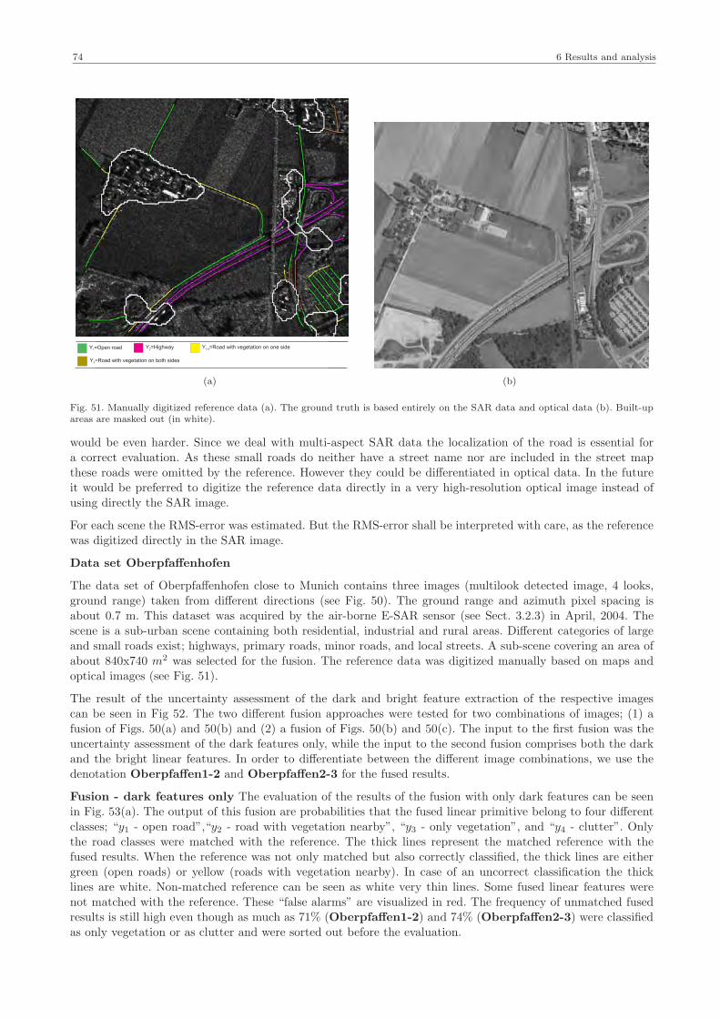
74 6 Results and analysis
Y =Open road1Y =Highway2 Y =Road with vegetation on one side3-4
Y =Road with vegetation on both sides5
(a) (b)
Fig. 51. Manually digitized reference data (a). The ground truth is based entirely on the SAR data and optical data (b). Built-upareas are masked out (in white).
would be even harder. Since we deal with multi-aspect SAR data the localization of the road is essential fora correct evaluation. As these small roads do neither have a street name nor are included in the street map
these roads were omitted by the reference. However they could be differentiated in optical data. In the future
it would be preferred to digitize the reference data directly in a very high-resolution optical image instead of
using directly the SAR image.
For each scene the RMS-error was estimated. But the RMS-error shall be interpreted with care, as the reference
was digitized directly in the SAR image.
Data set Oberpfaffenhofen
The data set of Oberpfaffenhofen close to Munich contains three images (multilook detected image, 4 looks,
ground range) taken from different directions (see Fig. 50). The ground range and azimuth pixel spacing isabout 0.7 m. This dataset was acquired by the air-borne E-SAR sensor (see Sect. 3.2.3) in April, 2004. The
scene is a sub-urban scene containing both residential, industrial and rural areas. Different categories of large
and small roads exist; highways, primary roads, minor roads, and local streets. A sub-scene covering an area ofabout 840x740 m2 was selected for the fusion. The reference data was digitized manually based on maps and
optical images (see Fig. 51).
The result of the uncertainty assessment of the dark and bright feature extraction of the respective imagescan be seen in Fig 52. The two different fusion approaches were tested for two combinations of images; (1) a
fusion of Figs. 50(a) and 50(b) and (2) a fusion of Figs. 50(b) and 50(c). The input to the first fusion was the
uncertainty assessment of the dark features only, while the input to the second fusion comprises both the darkand the bright linear features. In order to differentiate between the different image combinations, we use the
denotation Oberpfaffen1-2 and Oberpfaffen2-3 for the fused results.
Fusion - dark features only The evaluation of the results of the fusion with only dark features can be seenin Fig. 53(a). The output of this fusion are probabilities that the fused linear primitive belong to four different
classes; “y1 - open road”,“y2 - road with vegetation nearby”, “y3 - only vegetation”, and “y4 - clutter”. Only
the road classes were matched with the reference. The thick lines represent the matched reference with thefused results. When the reference was not only matched but also correctly classified, the thick lines are either
green (open roads) or yellow (roads with vegetation nearby). In case of an uncorrect classification the thick
lines are white. Non-matched reference can be seen as white very thin lines. Some fused linear features were
not matched with the reference. These “false alarms” are visualized in red. The frequency of unmatched fusedresults is still high even though as much as 71% (Oberpfaffen1-2) and 74% (Oberpfaffen2-3) were classified
as only vegetation or as clutter and were sorted out before the evaluation.
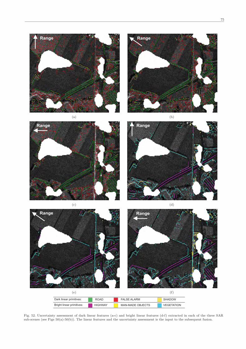
75
Range
(a)
Range
(b)
Range
(c)
Range
(d)
Range
(e)
Range
(f)
ROAD FALSE ALARM SHADOW
HIGHWAY MAN-MADE OBJECTS VEGETATION
Dark linear primitives:
Bright linear primitives:
Fig. 52. Uncertainty assessment of dark linear features (a-c) and bright linear features (d-f) extracted in each of the three SARsub-scenes (see Figs 50(a)-50(b)). The linear features and the uncertainty assessment is the input to the subsequent fusion.

76 6 Results and analysis
(a) (b)
Y =Open road1 Wrongly classified
Thick lines = matched reference: Thin lines
False extractionY =Road with vegetation2 Unmatched reference
Fig. 53. Results of the dataset Oberpfaffenhofen after fusion (BN3). Input to the fusion are the dark linear features and theiruncertainty assessment. Masked built-up areas are white. (a) Oberpfaffen1-2 shows the fusion of Figs. 52(a) and 52(b) while (b)Oberpfaffen2-3 shows the fusion of Figs. 52(b) and 52(c).
Fusion of Oberpfaffenhofen 1 and 2
Error Matrix
Y1 Y2 Total User’s Accuracy Producer’s Accuracy Overall Accuracy
y1 710 32 742 0.96 0.87
y2 102 98 200 0.51 0.75
Total 812 130 942 0.86
Quality Measures
Overall Completeness 0.70
Overall Correctness 0.60
RMS 4.1 m
Fusion of Oberpfaffenhofen 2 and 3
Error Matrix
Y1 Y2 Total User’s Accuracy Producer’s Accuracy Overall Accuracy
y1 773 85 858 0.90 0.92
y2 66 50 116 0.57 0.37
Total 839 135 974 0.84
Quality Measures
Overall Completeness 0.72
Overall Correctness 0.60
RMS 4.2 m
Tab. 12. Error matrix for the fused linear primitives (BN3 - only dark features) extracted from data set Oberpfaffenhofen. Allfused features classified into “y3 - only vegetation” and “y4 - clutter” were sorted out before matching. Capital letters indicate thereference and the classification results are referred to as the lowercase letters. Y1 means the reference class for open roads, Y2 is thereference class for roads with vegetation nearby.
Based on the error matrix (see Tab. 12) one can draw the conclusion that the fusion is able to identify the openroads very well. Both producer’s and user’s accuracies are high (about 90%) for both data sets. The results for
roads with vegetation nearby is not as high as for the open roads but still indeed acceptable for Oberpfaffen1-2
(user’s accuracy is 75% and producer’s accuracy is 83%). Unfortunately for Oberpfaffen2-3 the accuracies are

77
much lower. Interesting is that the main part of the fused linear primitives that was not matched with thereference (false extraction) were classified into roads with vegetation nearby. This is one more indicator of that
the classification of this class is not as reliable as for open roads.
Both datasets showed high completeness values, 70% and 72%. The correctness is a bit lower and was 60% for
both scenes. It was also tested to sort out only clutter, but then the overall completeness only increased by 4%
(Oberpfaffen1-2) and 5% (Oberpfaffen2-3) while the correctness became as low as 51% (Oberpfaffen1-2)and as 53% (Oberpfaffen2-3).
Based on Fig. 53 we can draw the conclusion that the fusion is able to detect open roads very well. Still thefusion has some problems to differentiate between only vegetation and roads with vegetation. Some shadow
regions close to the forest regions were wrongly assigned to one of the road classes. One explanation could be
the regular shape of the forest border. Hence the extracted line features become a high assessment of beingroads instead of shadows already before the fusion.
(a) (b)
(c)
Y =Open road1Y =Highway2
Y =Road with vegetation on one side3-4
Y =Road with vegetation on both sides5
Wrongly classified
Thick lines = matched reference:
Thin lines
Unmatched reference
False extraction
Fig. 54. The results after fusion based on the Bayesian network BN5 was matched with the reference. Input to the fusion are not onlythe dark but also the bright linear features and their uncertainty assessment. Masked built-up areas are white. (a) Oberpfaffen1-2shows the fusion of Figs. 52(a), 52(b), 52(d), and 52(e) while (b) Oberpfaffen2-3 shows the fusion of Figs. 52(b), 52(c), 52(e),and 52(f). (c) Oberpfaffen1-2 including prior information.
Fusion - bright features included The results of the fusion of both bright and dark features are visualizedin Fig. 54. The fused line primitives of this fusion are classified into as many as ten different classes. Five of
these are different road classes; “y1 - open roads”, “y2 - highways”, “y3−4 - road with vegetation on one side
of the road” and “y5 - road with vegetation on both sides of the road”. The remaining five are assumed to be

78 6 Results and analysis
false alarms; “y6−7 - only vegetation”, “y8−9 - only buildings” and “y10 - clutter”. Also in this case all falsealarm classes (y6 − y10) were sorted out before the fused linear primitives were matched with the reference. The
frequency of false alarms is even higher than for the previous fusion. But as much as 78% (Oberpfaffenhofen1-
2) and 87% (Oberpfaffenhofen2-3) of the linear features were classified into the false alarm classes, indicatingthat a strong selection already took place.
The overall completeness is high (77% - Oberpfaffenhofen1-2 and 73% - Oberpfaffenhofen2-3). If only
clutter is sorted out the completeness increases a bit, but not more than 5-7%. That indicates that the fusion
is indeed able to distinguish false from the true extraction.
Fusion of Oberpfaffenhofen 1 and 2
Error Matrix (without prior)
Y1 Y2 Y3−4 Y5 Total User’s Accuracy Producer’s Accuracy Overall Accuracy
y1 252 24 16 33 325 0.78 0.56
y2 153 296 7 0 456 0.65 0.72
y3−4 30 23 59 16 128 0.46 0.58
y5 13 66 19 39 137 0.28 0.44
Total 448 409 101 88 1046 0.62
Quality Measures without prior with prior
Overall Completeness 0.77 0.75
Overall Correctness 0.55 0.62
RMS 4.0 4.0
Fusion of Oberpfaffenhofen 2 and 3
Error Matrix
Y1 Y2 Y3−4 Y5 Total User’s Accuracy Producer’s Accuracy Overall Accuracy
y1 243 43 24 27 337 0.72 0.52
y2 200 291 8 11 510 0.57 0.80
y3−4 21 22 57 7 107 0.53 0.61
y5 0 10 5 26 41 0.63 0.37
Total 464 366 94 71 995 0.62
Quality Measures
Overall Completeness 0.73
Overall Correctness 0.53
RMS 4.3 m
Tab. 13. Error matrix for the fused linear primitives (BN5 - dark and bright features) extracted from data set Oberpfaffenhofen. Allfused features classified into “y6−7 - only vegetation”, “y8−9 - only buildings” and “y10 - clutter” were sorted out before matching.Capital letters indicate the reference and the classification results are referred to as the lowercase letters. Y1 means the referenceclass for open roads, Y2 is the reference class for roads with vegetation nearby.
The user’s and producer’s accuracies are not as high as for the fusion with only dark features (see Tab. 13).But one should also keep in mind that the number of classes are now ten instead of only four. Open roads and
highways are divided into two separated classes. Further roads with vegetation on one side and on both sides are
differentiated. Still the user’s accuracies and producer’s accuracies show acceptable values, especially for openroads and highways. The results may have been even better if not a small road would be so close to the highway.
Even an experienced user would think that the small road is a third lane of the highway. The fusion identifies
the road in both datasets as a part of the highway. Unfortunately the road is rather long and represents a large
part of the open road reference. An other interesting area is the parking lot. The parking lot is surrounded bylow vegetation and therefore the bright feature extraction has similar attributes as the bright highway linear
features. Unfortunately the user’s and producer’s accuracies for the class “y5 - road with vegetation on both
sides of the road” show rather low values. However these values cannot be considered as reliable since the classis rarely present in the reference set. An other reason is that the class is dependent on a good detection of both
dark and bright features. Shorter parts of the highway such as the highway cross are often falsely assigned to
roads with vegetation nearby because of the short length of the extracted bright and dark features.

79
If the two Figs 54(a) and 54(b) are compared, one can notice that the two fusions classify the diagonal roadin the middle differently. The fusion succeeds to identify the road as a road with vegetation nearby in the first
dataset, but in the second the fusion assumes that there is a road with vegetation also below the true road. The
reason for this is that the row of trees gives rise to a linear homogeneous shadow region. This region is detectedby the line extraction and later on obtains a high probability of being road. Since the two dark linear features
are too far away for being fused, each separately are assumed to be roads.
One way to reduce the false extraction is to introduce prior information as described in Sect. 5.6. By incor-porating the knowledge that the frequency of clutter is higher in forest areas, the correctness for the scene
Oberpfaffen1-2 could be increased by as much as 15%, while the completeness was only reduced by 3%. As
also stated in Sect. 5.6 the prior has an impact only on fused linear primitives with already a high assessmentof being clutter. The result can be seen in Fig. 54(c).
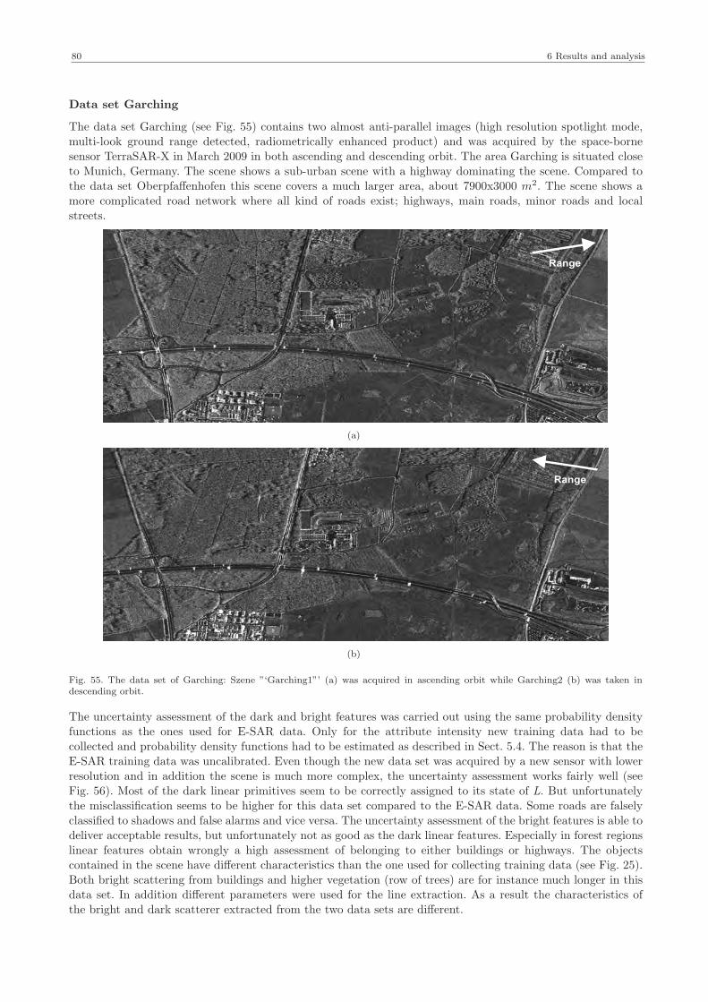
80 6 Results and analysis
Data set Garching
The data set Garching (see Fig. 55) contains two almost anti-parallel images (high resolution spotlight mode,
multi-look ground range detected, radiometrically enhanced product) and was acquired by the space-borne
sensor TerraSAR-X in March 2009 in both ascending and descending orbit. The area Garching is situated closeto Munich, Germany. The scene shows a sub-urban scene with a highway dominating the scene. Compared to
the data set Oberpfaffenhofen this scene covers a much larger area, about 7900x3000 m2. The scene shows a
more complicated road network where all kind of roads exist; highways, main roads, minor roads and localstreets.
Range
(a)
Range
(b)
Fig. 55. The data set of Garching: Szene ”‘Garching1”’ (a) was acquired in ascending orbit while Garching2 (b) was taken indescending orbit.
The uncertainty assessment of the dark and bright features was carried out using the same probability density
functions as the ones used for E-SAR data. Only for the attribute intensity new training data had to be
collected and probability density functions had to be estimated as described in Sect. 5.4. The reason is that theE-SAR training data was uncalibrated. Even though the new data set was acquired by a new sensor with lower
resolution and in addition the scene is much more complex, the uncertainty assessment works fairly well (see
Fig. 56). Most of the dark linear primitives seem to be correctly assigned to its state of L. But unfortunatelythe misclassification seems to be higher for this data set compared to the E-SAR data. Some roads are falsely
classified to shadows and false alarms and vice versa. The uncertainty assessment of the bright features is able to
deliver acceptable results, but unfortunately not as good as the dark linear features. Especially in forest regions
linear features obtain wrongly a high assessment of belonging to either buildings or highways. The objectscontained in the scene have different characteristics than the one used for collecting training data (see Fig. 25).
Both bright scattering from buildings and higher vegetation (row of trees) are for instance much longer in this
data set. In addition different parameters were used for the line extraction. As a result the characteristics ofthe bright and dark scatterer extracted from the two data sets are different.

81
Range
(a)
Range
(b)
Range
(c)
Range
(d)
ROAD FALSE ALARM SHADOW
HIGHWAY MAN-MADE OBJECTS VEGETATION
Dark linear primitives:
Bright linear primitives:
Fig. 56. Uncertainty assessment of dark linear features (a-b) and bright linear features (c-d) extracted in each of the two SARsub-scenes of Garching (see Figs 55(a)-55(b)). The linear features and the uncertainty assessment is the input to the subsequentfusion.

82 6 Results and analysis
The dark and bright features including their uncertainty assessment is the input to the subsequent fusion (BN5).The fused results matched with the reference for the data set Garching (see Fig. 57) can be seen in Fig. 58. One
can draw the conclusion from the quality measures presented in Tab. 14 that the fusion - despite the different
data characteristics - delivers acceptable results. The overall completeness are in the same range (74-77 %)as for the data set Oberpfaffenhofen. If only clutter is sorted out the completeness increases 12% and reaches
a completeness of 86%. However then the correctness decreases as much as 30%. The correctness values are
unfortunately lower (44-47%) compared to Oberpfaffenhofen. But we should keep in mind that our aim is toachieve rather higher completeness values than higher correctness values.
Y =Open road1Y =Highway2 Y =Road with vegetation on one side3-4
Y =Road with vegetation on both sides5
Fig. 57. Manually digitized reference for the data set Garching.
Y =Open road1Y =Highway2 Y =Road with vegetation on one side3-4
Y =Road with vegetation on both sides5 Wrongly classified
Thick lines = matched reference: Thin lines
Unmatched reference
False extraction
Fig. 58. Garching1-2: The results after fusion based on the Bayesian network BN5 was matched with the reference. Input to thefusion are not only the dark but also the bright linear features and their uncertainty assessment (see Fig. 56). Masked built-upareas are white.
The error matrix (see Tab. 14) shows that the fusion is able to classify most highways and most open roads
correctly. Both user’s and producer’s accuracies for these two classes are acceptable. Compared to Oberpfaf-
fenhofen we do not longer have the problem of open roads classified into highways. Here rather the oppositeoccur.
Again the fusion meets problem by the classification of the class “y3−4 - road with vegetation one side” Thereason for the rather poor classification is partly due to the mis-classification of bright features. As one can
see in Figs. 56(c)-56(d) some vegetation is falsely assessed to belong to highways. Second, the reference data
probably contains some errors since it was hard to estimate by means of optical data if there was vegetation on

83
Fusion of Garching 1 and 2
Error Matrix (without prior)
Y1 Y2 Y3−4 Y5 Total User’s Accuracy Producer’s Accuracy Overall Accuracy
y1 134 119 29 59 341 0.39 0.64
y2 1 581 97 72 751 0.77 0.67
y3−4 45 112 25 83 265 0.09 0.14
y5 29 49 27 143 248 0.58 0.40
Total 209 861 178 357 1605 0.55
Quality Measures without prior with prior
Overall Completeness 0.77 0.74
Overall Correctness 0.44 0.47
RMS 8.8 10.8
Tab. 14. Error matrix for the fused linear primitives (BN5 - dark and bright features) extracted from data set Garching. All fusedfeatures classified into “y6−7 - only vegetation”, “y8−9 - only buildings” and “y10 - clutter” were sorted out before matching.Capital letters indicate the reference and the classification results are referred to as the lowercase letters. Y1 means the referenceclass for open roads, Y2 is the reference class for roads with vegetation nearby.
both sides or not. Especially lower vegetation was hard to differentiate from the fields. These were detected inthe SAR data resulting that some line features assigned to y3−4 in the reference data were classified into y5 by
the fusion. An other reason was also that the conditional probability table behaves similar for the states y3−4 as
for the states “y6−7 - only vegetation”. Line features with the probability BEL(Y = y6−7) > BEL(Y = y1−5)
were sorted out before the matching and hence these parts are regarded as unmatched. We should keep inmind however that the classifier only gives us support by the seed point selection. For these line segments
BEL(Y = y3−4) is still high, meaning that these will most likely be involved in the subsequent shortest-path
calculation.
Fortunately the classifier is able to distinguish the class “y5 - road with vegetation on both sides” better than
for the data set Oberpfaffenhofen. The class is better represented among the reference data meaning that the
evaluation of this class should be regarded as more reliable as for Oberpfaffenhofen. Due to the same reasonsmentioned for y3−4 some linear features are wrongly assigned to be highways.
As can be seen in Fig. 58 the number of falsely extracted line primitives in forest regions is high. Most of
these (63%) got a high assessment of being open roads. The reason why open roads and clutter are harder todifferentiate is that these two are the only classes, which do not expect any bright feature extraction nearby. Also
for this data set prior information was incorporated. Indeed the correctness was then increased but unfortunately
the completeness was decreased at the same time. The fact that most of the falsely extracted line primitives wereassigned to open roads makes us more certain that the conditional probabilities are not optimally estimated for
the two classes open roads and clutter. But one should of course also keep in mind that the amount of clutter
detected in forest regions is already very high (see the dark line extraction in Figs. 56(a) and in 56(b)).
The overall accuracy (55%) is unfortunately lower than the accuracies presented for Oberpfaffenhofen. However
one should keep in mind that the fusion was primarily learned for E-SAR data and not for TerraSAR-X data.
Conclusions of results
Based on the results presented in this section we can draw the following conclusions:
⋄ By comparing the two fusions, the fusion for both bright and dark features (BN5) was able to deliver aslightly higher completeness. If also prior information was included the correctness increased slightly.
⋄ The fusion was also tested on multi-aspect SAR data acquired by a different sensor than the data used for
learning the fusion. Even though the new data set had both different data and scene characteristics thefusion could deliver acceptable results.
⋄ The quality measures presented give an indication that the behavior of the fusion is rather indulgent than
severe.
⋄ The error matrices show that the fusion delivers in general an overall result for the classification, but hassome difficulties by some classes. Certainly the fusion will be able to support the subsequent selection of
seed points for the network generation.

84 7 Conclusion and discussion
7 Conclusion and discussion
Summary
In this work, we have presented a fusion approach for automatic road extraction from multi-aspect SAR images.
We designed a probabilistic decision-level fusion for extracted linear features, which fully exploits multi-aspectSAR data. By means of Bayesian network theory a reasoning step could be modeled which describes the relation
between the extracted road, neighboring high objects and the sensor geometry. Also global context represent-
ing prior information was incorporated. The different steps; analyzing incoming information, structuring theBayesian networks, learning the fusion by means of training data, and the association step, were described in
detail.
Two different fusions were developed and tested; one developed for dark linear features only and one incorpo-
rating both dark and bright linear features. Those two were tested and compared on multi-aspect SAR data. Inaddition the fusion concept was tested on data acquired from different SAR sensors.
Discussion
Designing the fusion within Bayesian network theory enables us to fully exploit multi-aspect SAR data. The
advantage of using Bayesian network theory is that it offers us an optimal framework for dealing with relations.Hence the reasoning step required for the modeling of the relation between the road, neighboring objects and
the sensor geometry could be implemented. Furthermore it allows us to handle as much information as feature
extraction, road model, sensor geometry, and local and global context, due to its certain graph structure. Assoon as the structure is defined it is straight forward to estimate the flow of incoming and outgoing information.
However finding the optimal structure is the crucial and most important step and - depending on the task -
can be rather complicated. The dependencies/independencies among the variables are not always obvious. Onemight have to try different structures before a suitable one is found. Also in this work some structures were
tested before the final two proposed in this work were defined. An other disadvantage of Bayesian network is
that it requires a complete probabilistic model. Hence all possible states of each variable must be defined. The
more states, the more comprehensive is in general the learning. Estimating the conditional probabilities forthis application required training data. The collection was unfortunately time-consuming especially when many
states needed to be defined. If also parental or child nodes are correlated, the learning is even more complicated.
To simplify the learning a hidden node was implemented in this work (see Sect. 5.5.2).
Despite the complexity of setting up the structure and learning, Bayesian network is the optimal framework for
this work. The decisive point is that Bayesian network theory is the best suited decision-level fusion technique
for dealing with relations among so much different information. In addition Bayesian network enables us to
express this in a probabilistic framework.
The first fusion developed in this work concentrates on dark feature extraction, a road model and the sensor
geometry. The number of variables is lower compared to the second fusion and this makes the fusion structure
less complex. The implementation and the learning is relatively fast. Unfortunately this approach does not fullyexploit multi-aspect SAR images. Only one occlusion effect (shadows) is included in the modeling which means
that the fusion meets problems as soon as layover occlusions are present. However the second fusion includes
also layover meaning that information about neighboring objects is available. Not only the number of variables
needs to be increased, also the variables are partly extended with more states. Setting up the structure and thelearning is now much more complicated. But the advantage is that the second fusion gives us information about
different road classes and thereby delivering much more and complete information about the scene.
By testing the two fusions on the same data set it was proved that the second fusion could deliver a higheroverall completeness. The same test also showed us that the accuracies of the ability of the fusion to discriminate
between different road types were in general lower for the second fusion than for the first. The reason is that
the first fusion contains only two road classes, while the second fusion comprises five different road classes. In
addition the error matrices presented in Sect. 6 show us that most confusions occur among either highwaysand open roads or among road with vegetation on one side or road with vegetation on both sides. Since the
first fusion combines highways and open roads into one class (open road) and has only one category for road
with vegetation nearby, it is not strange that the producer’s and user’s accuracies are in general both higher forthe first fusion. But we should not forget that the second fusion tend to falsely classify more clutter in forest
regions to open roads. The number could be suppressed by incorporating prior information. But still it shows
that some conditional probabilities were not optimally estimated. Most probably some parameters within the

85
probabilistic modeling of the reasoning step of the road, local context and sensor geometry could be optimized.The setting of the subjective probabilities may play an important role in this issue.
An other drawback of the two fusions is that a fixed height of all nearby objects and a fixed width of all roads
are assumed. Of course these numbers vary highly in the real world, leading to an incorrect estimation of theimpact of the global sensor geometry. Certainly this may have lead to mis-classifications among the fused results,
in particular for roads with vegetation nearby.
The fusion was learned on data acquired by the E-SAR sensor. In order to check whether the learning could be
transferred to other SAR data, the second fusion was tested on TerraSAR-X data. Besides adjusting the learningfor a different intensity range, all other conditional probabilities remained. The results showed indeed that the
fusion was applicable on images with different data and scene characteristics, even though it is recommendable to
adjust some conditional probabilities for the specific SAR scene, especially if the data and scene characteristicsdiffer too heavily.
A direct and objective comparison between the results obtained by the old fuzzy-fusion and the new statistical
approach is hard to make. The reason is that the tuning of the parameters of the old system has such a
high impact that the expected end results may become arbitrary ”‘good”’ or ”‘bad”’ depending on the timeinvested in the parameter setting. The previous version required the user to set a high number of parameters
for different Fuzzy-functions. Nevertheless the new statistical fusion represent indeed a great improvement. It is
especially developed for multi-aspect SAR image and thereby delivers more informative results compared to theold one. The use of statistics makes the fusion more compatible. The output could be used and linked to other
probabilistic modules, for instance a Markov random field search similar to the one proposed by Tupin et al.
(1998). An other advantage is that the system has become more user-friendly. By using the proposed fusion - if
it is properly learned - reduces the number of adjustable parameters significantly.
The applied fusion was still not completely implemented in TUM-LOREX. The remaining step is to link the
output of the fusion to the last step, namely the network generation step. The output of the fusion shall support
the selection of especially good candidates for roads (i.e. the seed points). The selection of the seed pointsis a crucial and important step for the network generation. Even though this was still not tested, the results
presented in Sect. 6 are indeed an indicator of that the fusion will certainly be able to support the seed point
selection.
Future work
The discussion above points out some parts of the proposed fusion, which could be optimized. One is to include
the height of any nearby objects and the width of the road as variables in the Bayesian network. This would be
an interesting task, since we would now be dealing with not only hypotheses but also an estimation of numerical
values. These variables are most suited to be implemented in the second fusion, since it also involves the brightscattering. Second, the influence of the subjective probabilities should be tested. This can be done by varying
the subjective probabilities for isolated cases and examine how the belief in different classes will change. Such an
investigation would at the same time give an indication on how the clutter can be better modeled. Thereby it isexpected to achieve a higher correctness. The influence of the subjective probabilities could also be checked by
matching different fused results obtained by different subjective probabilities with the reference as carried out
in (Kim and Nevatia, 2003). By plotting the correctness and completeness in diagrams the optimal numericalvalue for the subjective probabilities could be found.
Even though the results obtained from the TerraSAR-X data set presented in Sect. 6 show that the fusion is
transferable, it also gave us an indication that some additional learning could be useful. The typical attributes
of the different states of variable L (D), roads, shadows and false alarms, and B might differ depending on thespecific scene characteristics. Therefore one might consider to incorporate a training step into TUM-LOREX. By
selecting some of the extracted line primitives and assigning them to the different states, the probability density
functions could be adjusted to that specific scene. Also there could be an option to adopt the performance ofthe line extractor. A training step would of course involve additional work by the user, but would probably not
exceed much the time needed for the parameter setting of the old system.
The fusion should also preferably be tested on more than two images. Assuming that the sensor geometry differs
enough so that the images can be regarded as independent, the extracted results from one or more additionalimages can be included using the product (compare with Eq. 28). Then the structure of the fusion would turn into
an expandable Bayesian network similar to the concept proposed by Kim and Nevatia (2003). The extension
of this fusion to an expandable Bayesian network is easily done in theory, but would need some time for the

86 7 Conclusion and discussion
implementation. The complexity would increase if extracted information from images with a slightly differentsensor geometry would be fused. At what point can one assume that extracted information from the two images
are correlated or not? Bayesian network is able to deal with correlated information by hidden nodes (Pearl,
1988). If and how hidden nodes could be applied in this case would be a question worth looking into.
Also simulated data based on SAR data effects (Balz and Stilla, 2009) or on SAR raw data (Guida et al.,
2008) could improve the learning. In particular simulated data could help to improve the road and local context
model, which is essential for the design of the conditional probability table.
The proposed Bayesian network fusion offers us the ability to easily integrate additional data, for instance
GIS-information or remote sensing data from other sensors, such as optical data. Since the SAR data and the
new information are independent, the data can be easily integrated as new variables. The learning needed forthe new variables can be carried out in a similar form as the one proposed in this work. The option can be
useful when for instance older optical data should be validated by recently acquired SAR data.
This work has indeed showed the potential of using Bayesian network theory for automatic object extraction fromSAR data and in particular for multi-aspect SAR data. A new high-level fusion approach especially designed
for SAR data has been developed. This or a similar fusion concept would certainly be suitable also to other
SAR applications than automatic road extraction in the future.

References 87
References
Amberg, V., Spigai, M., Coulon, M. and Marthon, P. (2005a): From road extraction to man-made object
discrimination in high resolution sar data, 4th international conference on Physics in Image and SignalProcessing, PSIP’2005 , Toulouse,, Proceedings of PSIP, 163–168.
Amberg, V., Spigai, M., Coulon, M. and Marthon, P. (2005b): Improvement of road extraction in high
resolution sar data by a context-based approach, IGARSS’05, Seoul, Proceedings of IGARSS.Asilo, S., Paringit, E., Casiwan, C., Collado, W., Mehdiyev, M., Hazarica, M., Samarakkon,
L. and Kamthonkiat, D. (2007): Fusion techniques for rice area mapping using multitemporal radarsat-1
images in pangasinan and nueva ecija, Proceedings of the 27th Asian Conference on Remote Sensing, Kuala
Lumpur, Malaysia.Auclair Fortier, M., Ziou, D., Armenakis, D. and Wang, S. (1999): Automated correction and updating
of road databases from high-resolution imagery, Technical report, Canadian Journal of Remote Sensing.
Balz, T. and Stilla, U. (2009): Hybrid gpu-based single- and double-bounce sar simulation, Geoscience andRemote Sensing, IEEE Transactions on 47(10): 3519 –3529.
Baumgartner, A., Eckstein, W., Mayer, H., Heipke, C., Ebner, H. and Ix, I. (1997a): Context-
supported road extraction, In: Automatic Extraction of Man-Made Objects from Aerial and Space Images(II), Birkh auser Verlag Basel, 299–308.
Baumgartner, A., Steger, C., Mayer, H. and Eckstein, W. (1997b): Multi-resolution, semantic objects,
and context for road extraction, In Semantic Modeling for the Acquisition of Topographic Information from
Images and Maps, Birkhauser Verlag, 140–156.Bentabet, L., Jodouin, S., Ziou, D. and Vaillancourt, J. (2003): Road vectors update using sar imagery:
a snake-based method, Geoscience and Remote Sensing, IEEE Transactions on 41(8): 1785–1803.
Binder, J., Koller, D., Russell, S. and Kanazawa, K. (1997): Adaptive probabilistic networks with hiddenvariables, Mach. Learn. 29(2-3): 213–244.
Bloch, I. (1996): Information combination operators for data fusion: a comparative review with classification,
Systems, Man and Cybernetics, Part A, IEEE Transactions on 26(1): 52–67.Bolter, R. (2001): Buildings from SAR: detection and reconstruction of buildings from multiple view high
resolution interferometric SAR data., PhD thesis, University of Graz, Austria.
Busch, A. (1994): Fast recognition of lines in digital images without user-supplied parameters, Band 2357,
SPIE, 91–97.Chaabouni Chouayak, H. and Datcu, M. (2010): Coarse-to-fine approach for urban area interpretation
using terrasar-x data, IEEE Geoscience and Remote Sensing Letters 7: 78–82.
Chanussot, J., Mauris, G. and Lambert, P. (1999): Fuzzy fusion techniques for linear features detectionin multitemporal sar images, Geoscience and Remote Sensing, IEEE Transactions on 37(3): 1292–1305.
Cumming, I. G. and Wong, F. H. (2005): Digital Processing of Synthetic Aperture Radar Data: Algorithms
and Implementation, Artech House Inc., Boston, London.Dekker, R. (2003): Texture analysis and classification of ers sar images for map updating of urban areas in
the netherlands, Geoscience and Remote Sensing, IEEE Transactions on 41(9): 1950–1958.
Dell’Acqua, F. and Gamba, P. (2001): Detection of urban structures in sar images by robust fuzzy clus-
tering algorithms: The example of street tracking, IEEE Transactions on Geoscience and Remote Sensing39(10): 2287–2297.
Dell’Acqua, F., Gamba, P. and Lisini, G. (2003): Improvements to urban area characterization using multi-
temporal and multiangle sar images, Geoscience and Remote Sensing, IEEE Transactions on 41(9): 1996–2004.Dell’Acqua, F., Gamba, P. and Lisini, G. (2004): Coregistration of multiangle fine spatial resolution sar
images, Geoscience and Remote Sensing Letters, IEEE 1(4): 237–241.
Dell’Acqua, F., Gamba, P. and Lisini, G. (2009): Rapid mapping of high resolution sar scenes, ISPRS Jour-nal of Photogrammetry and Remote Sensing 64(5): 482 – 489: Theme Issue: Mapping with SAR: Techniques
and Applications.
Ferrari, S. and Vaghi, A. (2006): Demining sensor modeling and feature-level fusion by bayesian networks,
Sensors Journal, IEEE 6(2): 471–483.Fritz, T. (2007): Terrasar-x ground segment level 1b product format specification, Technical report, Cluster
Applied Remote Sensing, German Aerospace Center.
Gamba, P., Hellwich, O. and Lombardo, P. (2005): Editorial board, Information Fusion 6(4): 189–192:Fusion of Remotely Sensed Data over Urban Areas.
Garcia, A. L. (2000): Numerical Methods for Physics (2nd Edition), Prentice-Hall, Inc., Upper Saddle River,
NJ, USA: Artist-(cover), John Christiana and Designed By-(cover), Bruce Kenselaar.

88 References
Gerke, M., Butenuth, M., Heipke, C. and Willrich, F. (2004): Graph-supported verification of roaddatabases, ISPRS Journal of Photogrammetry and Remote Sensing 58(3-4): 152 – 165: Integration of Geodata
and Imagery for Automated Refinement and Update of Spatial Databases.
Gonzalez, R. C. and Woods, R. E. (2001): Digital Image Processing, Addison-Wesley Longman PublishingCo., Inc., Boston, MA, USA.
Guida, R., Iodice, A., Riccio, D. and Stilla, U. (2008): Model-based interpretation of high-resolution sar
images of buildings, Selected Topics in Applied Earth Observations and Remote Sensing, IEEE Journal of1(2): 107–119.
Hall, D. L. (1992): Mathematical Techniques in Multisensor Data Fusion, Artech House, Inc., Norwood, MA,
USA.
Hall, D. L. and Llinas, J. (2001): Handbook of Multisensor Data Fusion, CRC Press LLC, chapter MultisensorData Fusion.
Hedman, K., Hinz, S. and Stilla, U. (2006a): A probabilistic fusion concept for road extraction from multiple
sar views, Proc. 6th European conference on synthetic aperture radar, EUSAR 2006.Hedman, K., Hinz, S. and Stilla, U. (2006b): A probabilistic fusion strategy applied to road extraction from
multi-aspect sar data, Symposium of ISPRS Commission III: Photogrammetric Computer Vision (PCV06).
International Archives of Photogrammetry, Remote Sensing, and Spatial Information Sciences, Band 36, 55–60.
Hedman, K., Hinz, S. and Stilla, U. (2007): Road extraction from sar multi-aspect data supported by a
statistical context-based fusion, Urban Remote Sensing Joint Event: URBAN 2007 -URS 2007, 1–6.
Hedman, K., Stilla, U., Lisini, G. and Gamba, P. (2008): Road network extraction in urban areas by meansof feature-level fusion, 3. TerraSAR-X Science Team Meeting.
Hedman, K., Stilla, U., Lisini, G. and Gamba, P. (2010): Road network extraction in vhr sar images of
urban and suburban areas by means of class-aided feature-level fusion, IEEE Transactions on Geoscience andRemote Sensing 48(3): 1294–1296.
Hedman, K., Wessel, B. and Stilla, U. (2005a): A fusion strategy for extracted road networks from multi-
aspect sar images, in U. Stilla, F. Rottensteiner and F. Hinz (Herausgeber), CMRT05 InternationalArchives of Photogrammetry and Remote Sensing, Band 36, 185–190.
Hedman, K., Wessel, B., Stilla, U. and Soergel, U. (2005b): Automatic road extraction by fusion of
multiple sar views, in M. Moeller and E. Wentz (Herausgeber), 3th International Symposium: Remote
sensing and data fusion on urban areas, URBAN 2005. International Archives of Photogrammetry and RemoteSensing, Band 36, on CD.
Heipke, C., Mayer, H., Wiedemann, C. and Jamet, O. (1997): Evaluation of automatic road extraction,
In: International Archives of Photogrammetry and Remote Sensing, 47–56.Hellwich, O. (1996): Linienextraktion aus SAR-Daten mit einem Markoff-Zufallsfeld-Modell, PhD thesis,
Technische Universitat Munchen.
Hinz, S. (2004): Automatische Extraktion urbaner Straßennetze aus Luftbildern, PhD thesis, Technische Uni-versitat Munchen.
Hinz, S. and Baumgartner, A. (2003): Automatic extraction of urban road networks from multi-view aerial
imagery, ISPRS Journal of Photogrammetry and Remote Sensing 58(1-2): 83 – 98: Algorithms and Techniques
for Multi-Source Data Fusion in Urban Areas.Horn, R. (1996): The dlr airborne sar project e-sar, Proceedings of International Geoscience and Remote
Sensing Symposium, 1624–1628.
Jaynes, E. T. (2003): Probability Theory; the logic of science, Cambridge University Press.Jensen, F. V. (1996): An introduction to Bayesian networks, UCL Press: ISBN 1-85728-332-5.
Jeon, B.-K., Jang, J.-H. and Hong, K.-S. (2002): Road detection in spaceborne sar images using a genetic
algorithm, Geoscience and Remote Sensing, IEEE Transactions on 40(1): 22–29.Junghans, M. and Jentschel, H.-J. (2007): Qualification of traffic data by bayesian network data fusion,
Information Fusion, 2007 10th International Conference on 1–7.
Kim, Z. and Nevatia, R. (2003): Expandable bayesian networks for 3d object description from multiple views
and multiple mode inputs, Pattern Analysis and Machine Intelligence, IEEE Transactions on 25(6): 769–774.Kim, Z. and Nevatia, R. (2004): Automatic description of complex buildings from multiple images, Computer
Vision and Image Understanding 96(1): 60–95.
Larkin, M. (1998): Sensor fusion and classification of acoustic signals using bayesian networks, Signals, Systems& Computers, 1998. Conference Record of the Thirty-Second Asilomar Conference on 2: 1359–1362 vol.2.
Levitt, S. and Aghdasi, F. (2000): Fuzzy representation and grouping in building detection, Image Processing,
2000. Proceedings. 2000 International Conference on, Band 3, 324–327 vol.3.

References 89
Lillesand, Thomas, M., Kiefer, Ralph, W. and Chipman, W. J. (2008): Remote Sensing and ImageInterpretation, 6 edn, John Wiley & Sons, Inc.
Limpert, E., Stahel, W. A. and Abbt, M. (2001): Log-normal distributions across the sciences: Keys and
clues, BioScience 51(5): 341–352.Lisini, G., Tison, C., Tupin, F. and Gamba, P. (2006): Feature fusion to improve road network extraction
in high-resolution sar images, Geoscience and Remote Sensing Letters, IEEE 3(2): 217–221.
Lombardo, P., Oliver, C., Pellizzeri, T. and Meloni, M. (2003): A new maximum-likelihood joint seg-mentation technique for multitemporal sar and multiband optical images, IEEE Transactions on Geoscience
and Remote Sensing 41(11): 2500–2518.
Massonnet, D. and Souyris, J.-C. (2008): Imaging with Synthetic Aperture Radar, CRC Press, Taylor &
Francis Group.Mayer, H., Hinz, S., Bacher, U. and Baltsavias, E. (2006): A test of automatic road extraction approaches,
Symposium of ISPRS Commission III: Photogrammetric Computer Vision (PCV06). International Archives
of Photogrammetry, Remote Sensing, and Spatial Information Sciences, xx–yy.Negri, M., Gamba, P., Lisini, G. and Tupin, F. (2006): Junction-aware extraction and regularization of
urban road networks in high-resolution sar images, Geoscience and Remote Sensing, IEEE Transactions on
44(10): 2962 –2971.Pearl, J. (1988): Probabilistic Reasoning in Intelligent Systems : Networks of Plausible Inference, Morgan
Kaufmann.
Pearl, J. (2000): Causality: model, resoning, and inference, Cambridge University Press.
Pohl, C. and Van Genderen, J. L. (1998): Multisensor image fusion in remote sensing: concepts, methodsand applications, International Journal of Remote Sensing 19(5): 823–854.
Price, K. (1999): Road grid extraction and verification, International Archives of Photogrammetry and Remote
Sensing, Band XXXII, Part 3-2W5, 101–106.Roth, A., Hoffmann, J. and Esch, T. (2005): Terrasar-x: How can high resolution sar data support the
observation of urban areas?, ISPRS Joint Conference URBAN2005 and URS2005.
Shimazaki, H. and Shinomoto, S. (2007): A method for selecting the bin size of a time histogram, NeuralComputation 19(6): 1503–1527.
Soergel, U., Cadario, E. and Thoennessen, U. (2004): Geocoding and fusion of airborne high-resolution
multi-aspect sar-data, Proc. 5th European Conference on Synthetic Aperture Radara, EUSAR 2004, 945–948.
Soergel, U., Michaelsen, E., Thiele, A., Cadario, E. and Thoennessen, U. (2009): Stereo analysis ofhigh-resolution sar images for building height estimation in cases of orthogonal aspect directions, ISPRS Jour-
nal of Photogrammetry and Remote Sensing 64(5): 490 – 500: Theme Issue: Mapping with SAR: Techniques
and Applications.Soergel, U., Thoennessen, U. and Stilla, U. (2003): Visibility analysis of man-made objects in sar images,
IEEE Geoscience and Remote Sensing Society: 2nd GRSS/ISPRS Joint Workshop on Remote Sensing and
Data Fusion over Urban Areas, URBAN 2003, 120–124.Steger, C. (1998a): An unbiased detector of curvilinear structures, Pattern Analysis and Machine Intelligence,
IEEE Transactions on 20(2): 113–125.
Steger, C. (1998b): Unbiased Extraction of Curvilinear Structures from 2D and 3D images, PhD thesis,
Technische Universitat Munchen.Steger, C., Mayer, H. and Radig, B. (1997): The role of grouping for road extraction, In: Automatic
Extraction of Man-Made Objects from Aerial and Space Images (II), Birkh auser Verlag Basel, Verlag, 245–
256.Steinberg, A. N., Bowman, C. and White, J. F. E. (1998): Revisions to the jdl data fusion model, Proc.
3rd NATO/IROS Conf., Quebec City, Canada.
Stilla, U. (2007): High resolution radar imaging of urban areas, in D. Fritsch (Herausgeber), Photogram-metric Week 07, Wichmann: Heidelberg.
Stilla, U. and Hedman, K. (2010): Feature fusion based on Bayesian network theory for automatic road
extraction, Band 15, Springer, chapter 3, 69–86.
Stilla, U. and Soergel, U. (2006): Urban Remote Sensing, Taylor & Francis, CRC Press Inc., chapterReconstruction of Buildings in SAR Imagery of Urban Areas, 47–68.
Stilla, U., Hinz, S., Hedman, K. and Wessel, B. (2007): Remote Sensing of Impervious Surfaces, Remote
Sensing Application Series, CRC Press, Taylor & Francis, chapter Road extraction from SAR imagery.Stilla, U., Soergel, U. and Thoennessen, U. (2003): Potential and limits of insar data for building re-
construction in built-up areas, ISPRS Journal of Photogrammetry and Remote Sensing 58(1-2): 113 – 123:
Algorithms and Techniques for Multi-Source Data Fusion in Urban Areas.

90 References
Sun, G. and Ranson, K. (1995): A three-dimensional radar backscatter model of forest canopies, Geoscienceand Remote Sensing, IEEE Transactions on 33(2): 372–382.
Thiele, A., Cadario, E., Schulz, K. and Soergel, U. (2010): Analysis of gable-roofed building signature
in multiaspect insar data, Geoscience and Remote Sensing Letters, IEEE 7(1): 83 –87.Thiele, A., Cadario, E., Schulz, K., Thonnessen, U. and Soergel, U. (2007): Building recognition from
multi-aspect high-resolution insar data in urban areas, Geoscience and Remote Sensing, IEEE Transactions
on 45(11): 3583–3593.Tison, C., Nicolas, J.-M., Tupin, F. and Maitre, H. (2004): A new statistical model for markovian
classification of urban areas in high-resolution sar images, Geoscience and Remote Sensing, IEEE Transactions
on 42(10): 2046–2057.
Touzi, R. (2002): A review of speckle filtering in the context of estimation theory, Geoscience and RemoteSensing, IEEE Transactions on 40(11): 2392–2404.
Touzi, R., Lopez, A. and Bousquet, P. (1988): A statistical and geometrical edge detector for sar images,
IEEE Transactions on Geoscience and Remote Sensing 26(6): 764–773.Tupin, F. (2000): Radar cross-views for road detection in dense urban areas, Proc. EUSAR 2000, Munich,
Germany, 617–620.
Tupin, F. (2010): Radar Remote Sensing of Urban Areas, Band 15 of Remote Sensing and Digital ImageProcessing, Springer, chapter Fusion of optical and SAR images, 133–159.
Tupin, F., Bloch, I. and Maitre, H. (1999): A first step toward automatic interpretation of sar images
using evidential fusion of several structure detectors, Geoscience and Remote Sensing, IEEE Transactions on
37(3): 1327–1343.Tupin, F., Houshmand, B. and Datcu, M. (2002): Road detection in dense urban areas using sar imagery and
the usefulness of multiple views, Geoscience and Remote Sensing, IEEE Transactions on 40(11): 2405–2414.
Tupin, F., Maitre, H., Mangin, J.-F., Nicolas, J.-M. and Pechersky, E. (1998): Detection of linearfeatures in sar images: application to road network extraction, Geoscience and Remote Sensing, IEEE Trans-
actions on 36(2): 434–453.
Ulaby, F., Moore, R. K. and Fung, A. K. (1982): Radar Remote Sensing and Surface Scattering and Emis-sion Theory, Band Band II of Microwave Remote Sensing: Active and Passive, Addison-Wesley Publishing
Company, Reading, MA.
Wald, L. (1998): An overview of concepts in fusion of earth data, Future Trends in Remote Sensing, EARSeL
Symposium 1997, Lyngby, Denmark, Nummer 385-390.Wald, L. (1999): Some terms of reference in data fusion, IEEE Transactions on Geoscience and Remote Sensing
13(3): 1190–1193.
Wald, L. (2002): Data Fusion, Definitions and Architectures, Fusion of images of different spatial resolutions,Les Presses de l’Ecole des Mines.
Waltz, E. (2001): Handbook of Multisensor Data Fusion, CRC Press LLC, chapter The Principles and Practice
of Image and Spatial Data Fusion.Waske, B. and Benediktsson, J. (2007): Fusion of support vector machines for classification of multisensor
data, IEEE Transactions on Geoscience and Remote Sensing 45(12): 3858–3866.
Waske, B. and van der Linden, S. (2008): Classifying multilevel imagery from sar and optical sensors by
decision fusion, IEEE Transactions on Geoscience and Remote Sensing 46(5): 1457–1466.Weidner, U. and Centeno, J. A. S. (2009): Pansharpening - simple approaches and their evaluation, Pho-
togrammetrie - Fernerkundung - Geoinformation 2009(4): 317–327.
Wessel, B. (2004): Road network extraction from sar imagery supported by context information, XXth ISPRSCongress, Istanbul, International Archives of Photogrammetry and Remote Sensing.
Wessel, B. (2006): Automatische Extraktion von Straßen aus SAR-Bilddaten, PhD thesis, Technische Univer-
sitat Munchen.Wessel, B. and Hinz, S. (2004): Context-supported road extraction from sar imagery:transition from rural to
built-up areas, Proceedings of EUSAR ’04, Ulm.
Wessel, B. and Wiedemann, C. (2005): Analysis of automatic road extraction results from airborne sar
imagery, Proceedings of the ISPRS Conference Photogrammetric Image Analysis, Band 34, 105–110.Wiedemann, C. (2002): Extraktion con Straßennetzen aus optischen Satellitenbilddaten, PhD thesis, Technische
Universitat Munchen.
Wiedemann, C. and Ebner, H. (2000): Automatic completion and evaluation of road networks, In: Interna-tional Archives of Photogrammetry and Remote Sensing, 979–986.
Wiedemann, C. and Hinz, S. (1999): Automatic extraction and evaluation of road networks from satellite
imagery, International Archives of Photogrammetry and Remote Sensing, 95–100.

References 91
Zhang, J. (2010): Multi-source remote sensing data fusion: status and trends, International Journal of Imageand Data Fusion 1(1): 5–24.
Ziou, D. (2000): Optimal line detector, Pattern Recognition, International Conference on 3: 3534.

Acknowledgements
My sincere thanks go to my two doctoral advisers Prof. Dr.-Ing. Stefan Hinz and Prof. Dr.-Ing. Uwe Stilla.
Thanks to Prof. Stilla for giving me the opportunity to start my Thesis at Photogrammetry and RemoteSensing, Technische Universitat Munchen (TUM). He was also the one who gave me the first inputs to this
topic. Despite heavy workload and time pressure he took his time for fruitful discussions. I am also glad that
he continued to support me even though I changed my place of work to the Institute of Astronomical andPhysical Geodesy in 2006. Thanks to Prof. Hinz for giving me useful guidance and for supporting me to get
out of dead-ends at times. His inputs and ideas, both for small and big things, were very helpful for this work.
Without his knowledge and experience in this topic I would never have gotten this far. Thanks also for theintensive support and useful comments in the very end.
Many thanks also to Prof. Dr.-Ing. Hans-Peter Bahr for his willingness to support my work with such a short
notice.
I am also grateful to Dr.-Ing. Birgit Wessel for her advising during the first year. She was the one who introduced
the work with automatic road extraction from SAR. Without her and her knowledge in SAR and road extraction
it would have taken a long time before I got familiar with this topic.
A special thanks goes to Prof. Gamba and Dr. Gianni Lisini for supporting me during my research stay at
Universita di Pavia, Pavia, Italy. Thanks to them I learned a lot about their research in the field of automatic
road extraction and SAR data. Also thanks to Prof. Riccio and to my dear friend Dr. Raffaella Guida for thetime at Universita Federico II di Napoli, in Naples, Italy.
My next thanks go to all my former colleagues at the Institute of Photogrammetry and Cartography, TUM.
Thanks to Stefan Gernhardt for supporting me with the SAR data and thanks to Stefan Auer for helpingme with the reference data. Also a special thank to Christine Elmauer for everything she did. I am especially
grateful to my colleagues Andreas Laika, Jens Leitloff and Diana Weihing. Their support in both personal and
professional issues made me enjoying my time at TUM.
I would also like to express my gratitude to all my colleagues at the Institute of Astronomical and Physical
Geodesy (IAPG), TUM. First of all to Prof. Dr.-Ing. Reiner Rummel for giving me such freedom for organizing
my work so that I could find time for doing research. His support was very valuable to me. Next I would like tothank Prof. Dr.-Ing. Florian Seitz for the same reason. Due to his support and understanding during the busiest
period I was able to finish in such a short time. Also special thanks to Mary Fletcher for her understanding.
Last but not least I would like to thank my dear family and friends. No matter living in Sweden or in Germanyor somewhere else in the world, all of them have always been there for me. A special thanks to my mom, who
has taught me to strive hard for my goals. Many thanks to my dear Martin for his understanding for all my
busy working weekends and late nights. I hope that I some day can make up for it.

Curriculum Vitae
Name: Karin Helena Margareta Hedman
Place of Birth: Karlstad, Sweden
Date of Birth: June, 04, 1979
Educational background:
1995 — 1998 A-levels (school leaving exams) at Sundsta-Alvkullegymnasiet, Karlstad, Sweden
1999 — 2004 Master of Science in Space Engineering, Lulea University of Technology, Sweden
2001 Exchange studies at Nanyang Technological University, Singapore
Professional experience:
2004 — 2006 Scientific collaborator at Department of Photogrammetry and Remote Sensing,Technische Universitat Munchen
Since 2006 Scientific collaborator at Institute of Astronomical and Physical Geodesy,Technische Universitat MunchenProgram coordinator and student academic advisor for the internationalMaster’s program ”Earth Oriented Space Science and Technology” (ESPACE)