STATISTICS 479/503TIME SERIES ANALYSIS PART II

Doug WiensApril 12, 2005

Contents

II Time Domain Analysis 38

5 Lecture 5 . . . . . . . . . . . . . . . . . . . 39

6 Lecture 6 . . . . . . . . . . . . . . . . . . . 47

7 Lecture 7 . . . . . . . . . . . . . . . . . . . 56

8 Lecture 8 . . . . . . . . . . . . . . . . . . . 62

9 Lecture 9 . . . . . . . . . . . . . . . . . . . 71

37

10 Lecture 10 . . . . . . . . . . . . . . . . . . 78

11 Lecture 11 . . . . . . . . . . . . . . . . . . 87

12 Lecture 12 . . . . . . . . . . . . . . . . . . 97

13 Lecture 13 . . . . . . . . . . . . . . . . . . 115

14 Lecture 14 (Review) . . . . . . . . . . . . . 126

38

Part II

Time Domain Analysis

39

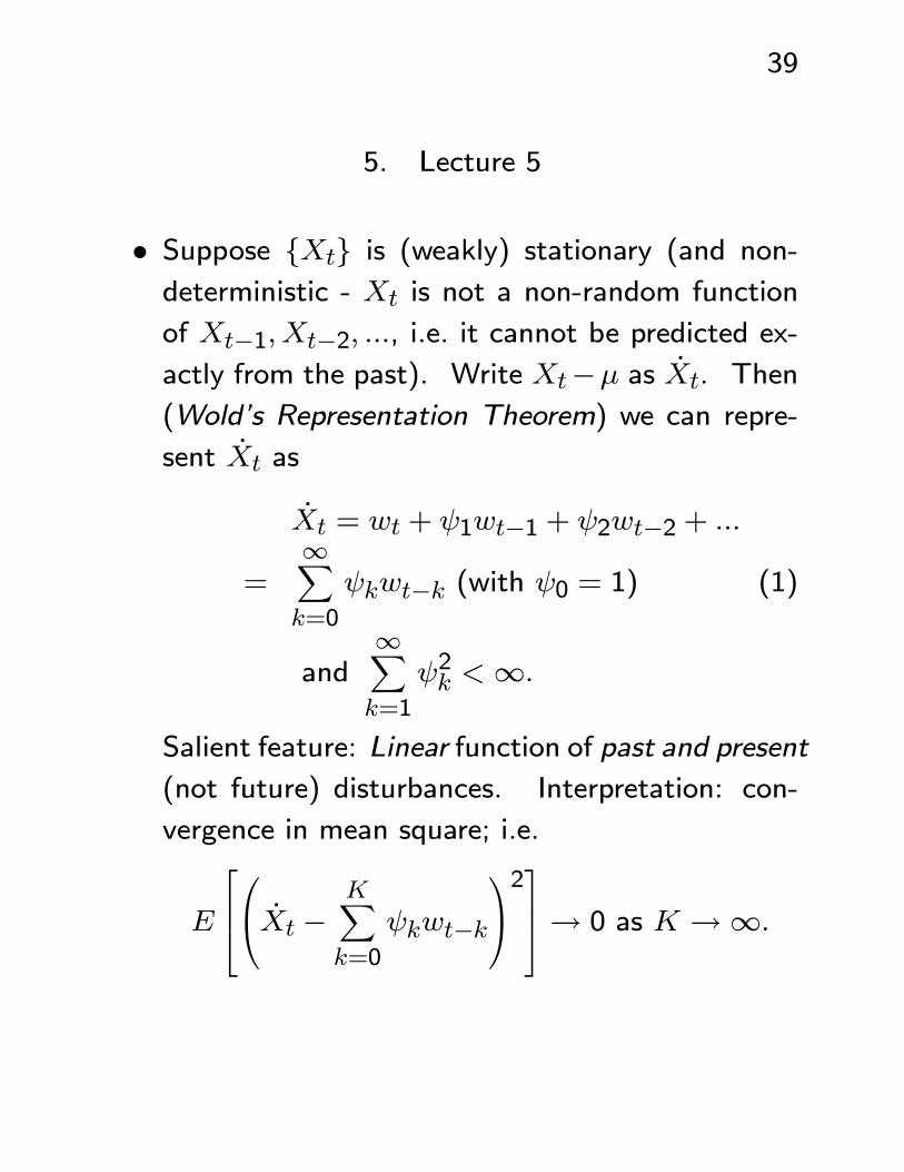
5. Lecture 5

• Suppose {Xt} is (weakly) stationary (and non-deterministic - Xt is not a non-random function

of Xt−1,Xt−2, ..., i.e. it cannot be predicted ex-actly from the past). Write Xt−µ as Xt. Then

(Wold’s Representation Theorem) we can repre-

sent Xt as

Xt = wt + ψ1wt−1 + ψ2wt−2 + ...

=∞Xk=0

ψkwt−k (with ψ0 = 1) (1)

and∞Xk=1

ψ2k <∞.

Salient feature: Linear function of past and present

(not future) disturbances. Interpretation: con-

vergence in mean square; i.e.

E

⎡⎢⎣⎛⎝Xt −

KXk=0

ψkwt−k

⎞⎠2⎤⎥⎦→ 0 as K →∞.

40

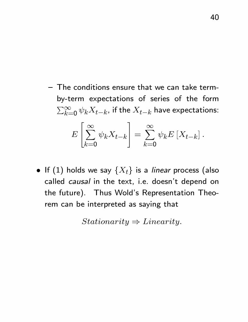
— The conditions ensure that we can take term-

by-term expectations of series of the formP∞k=0ψkXt−k, if the Xt−k have expectations:

E

⎡⎣ ∞Xk=0

ψkXt−k

⎤⎦ = ∞Xk=0

ψkE£Xt−k

¤.

• If (1) holds we say {Xt} is a linear process (alsocalled causal in the text, i.e. doesn’t depend on

the future). Thus Wold’s Representation Theo-

rem can be interpreted as saying that

Stationarity ⇒ Linearity.

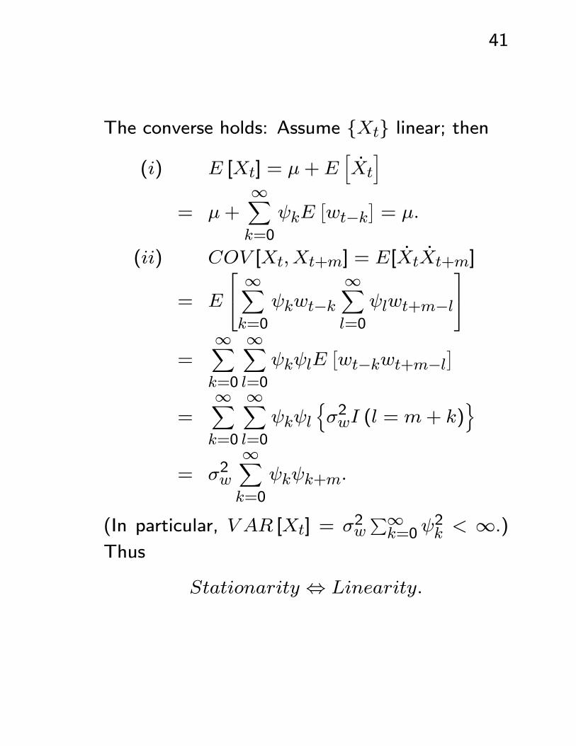
41

The converse holds: Assume {Xt} linear; then

(i) E [Xt] = µ+EhXt

i= µ+

∞Xk=0

ψkE£wt−k

¤= µ.

(ii) COV [Xt,Xt+m] = E[XtXt+m]

= E

⎡⎣ ∞Xk=0

ψkwt−k∞Xl=0

ψlwt+m−l

⎤⎦=

∞Xk=0

∞Xl=0

ψkψlE£wt−kwt+m−l

¤=

∞Xk=0

∞Xl=0

ψkψlnσ2wI (l = m+ k)

o= σ2w

∞Xk=0

ψkψk+m.

(In particular, V AR [Xt] = σ2wP∞k=0ψ

2k < ∞.)

Thus

Stationarity ⇔ Linearity.

42

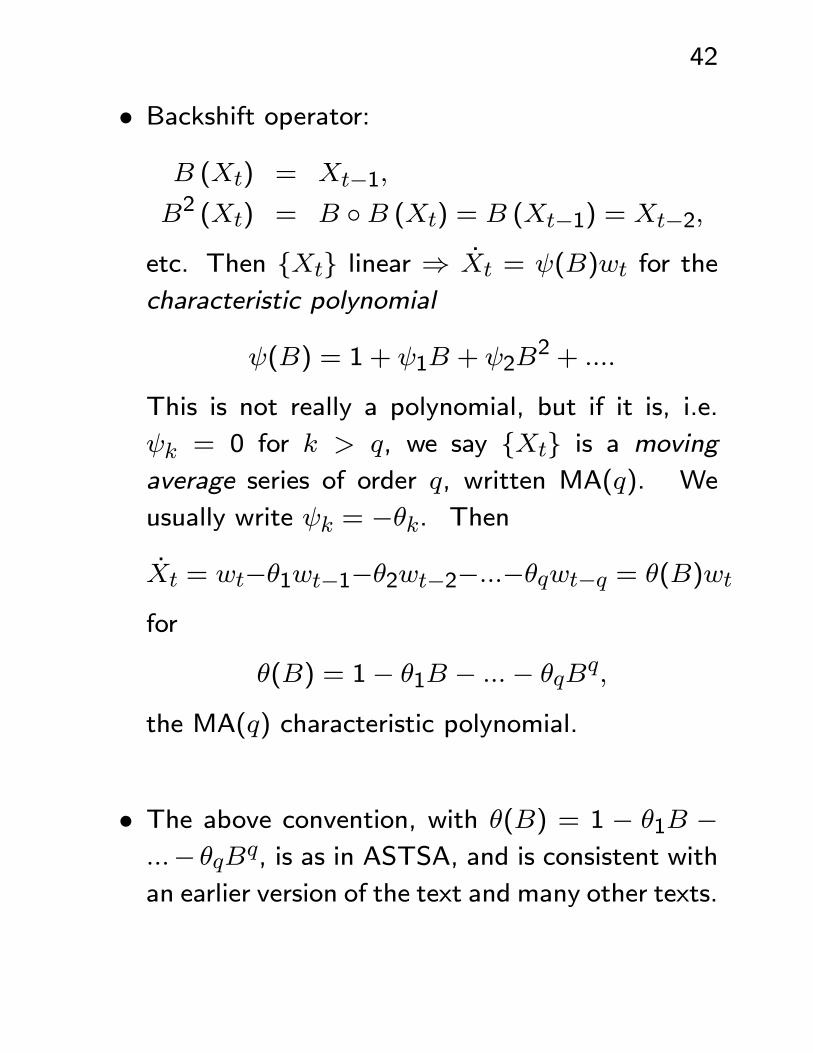
• Backshift operator:

B (Xt) = Xt−1,

B2 (Xt) = B ◦B (Xt) = B (Xt−1) = Xt−2,

etc. Then {Xt} linear ⇒ Xt = ψ(B)wt for the

characteristic polynomial

ψ(B) = 1 + ψ1B + ψ2B2 + ....

This is not really a polynomial, but if it is, i.e.

ψk = 0 for k > q, we say {Xt} is a movingaverage series of order q, written MA(q). We

usually write ψk = −θk. Then

Xt = wt−θ1wt−1−θ2wt−2−...−θqwt−q = θ(B)wt

for

θ(B) = 1− θ1B − ...− θqBq,

the MA(q) characteristic polynomial.

• The above convention, with θ(B) = 1 − θ1B −...− θqBq, is as in ASTSA, and is consistent with

an earlier version of the text and many other texts.

43

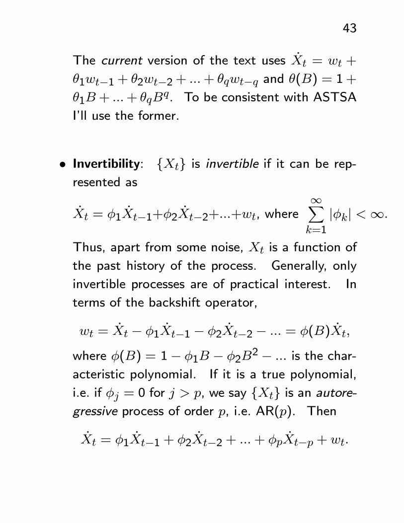
The current version of the text uses Xt = wt +

θ1wt−1 + θ2wt−2 + ...+ θqwt−q and θ(B) = 1+θ1B+ ...+ θqBq. To be consistent with ASTSA

I’ll use the former.

• Invertibility: {Xt} is invertible if it can be rep-resented as

Xt = φ1Xt−1+φ2Xt−2+...+wt, where∞Xk=1

|φk| <∞.

Thus, apart from some noise, Xt is a function of

the past history of the process. Generally, only

invertible processes are of practical interest. In

terms of the backshift operator,

wt = Xt − φ1Xt−1 − φ2Xt−2 − ... = φ(B)Xt,

where φ(B) = 1− φ1B − φ2B2− ... is the char-

acteristic polynomial. If it is a true polynomial,

i.e. if φj = 0 for j > p, we say {Xt} is an autore-gressive process of order p, i.e. AR(p). Then

Xt = φ1Xt−1 + φ2Xt−2 + ...+ φpXt−p +wt.

44

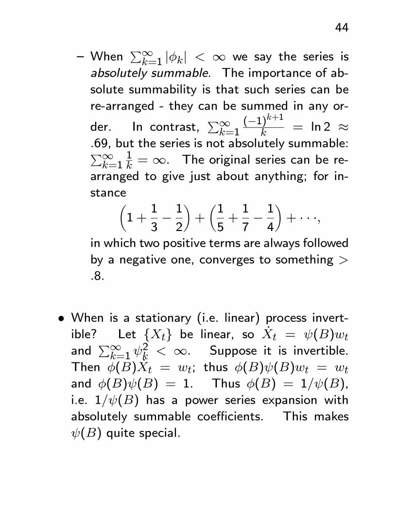
— WhenP∞k=1 |φk| < ∞ we say the series is

absolutely summable. The importance of ab-

solute summability is that such series can be

re-arranged - they can be summed in any or-

der. In contrast,P∞k=1

(−1)k+1k = ln 2 ≈

.69, but the series is not absolutely summable:P∞k=1

1k = ∞. The original series can be re-

arranged to give just about anything; for in-

stanceµ1 +

1

3− 12

¶+µ1

5+1

7− 14

¶+ · · ·,

in which two positive terms are always followed

by a negative one, converges to something >

.8.

• When is a stationary (i.e. linear) process invert-ible? Let {Xt} be linear, so Xt = ψ(B)wt

andP∞k=1ψ

2k < ∞. Suppose it is invertible.

Then φ(B)Xt = wt; thus φ(B)ψ(B)wt = wt

and φ(B)ψ(B) = 1. Thus φ(B) = 1/ψ(B),

i.e. 1/ψ(B) has a power series expansion with

absolutely summable coefficients. This makes

ψ(B) quite special.

45

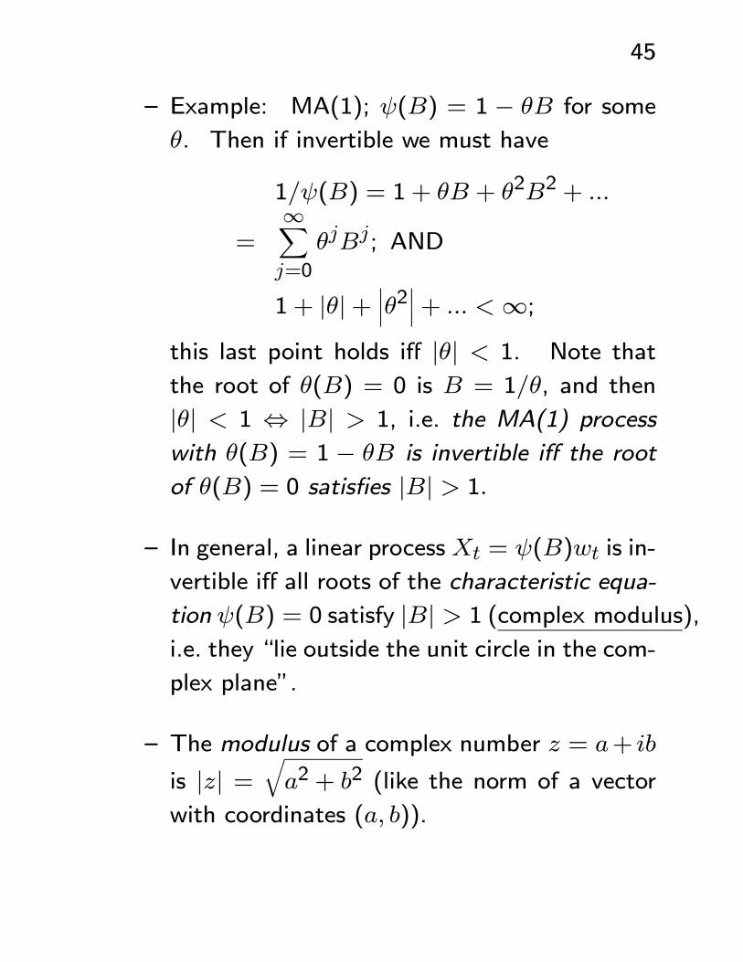
— Example: MA(1); ψ(B) = 1 − θB for some

θ. Then if invertible we must have

1/ψ(B) = 1 + θB + θ2B2 + ...

=∞Xj=0

θjBj; AND

1 + |θ|+¯θ2¯+ ... <∞;

this last point holds iff |θ| < 1. Note that

the root of θ(B) = 0 is B = 1/θ, and then

|θ| < 1 ⇔ |B| > 1, i.e. the MA(1) process

with θ(B) = 1 − θB is invertible iff the root

of θ(B) = 0 satisfies |B| > 1.

— In general, a linear processXt = ψ(B)wt is in-

vertible iff all roots of the characteristic equa-

tion ψ(B) = 0 satisfy |B| > 1 (complex modulus),

i.e. they “lie outside the unit circle in the com-

plex plane”.

— The modulus of a complex number z = a+ ib

is |z| =qa2 + b2 (like the norm of a vector

with coordinates (a, b)).

46

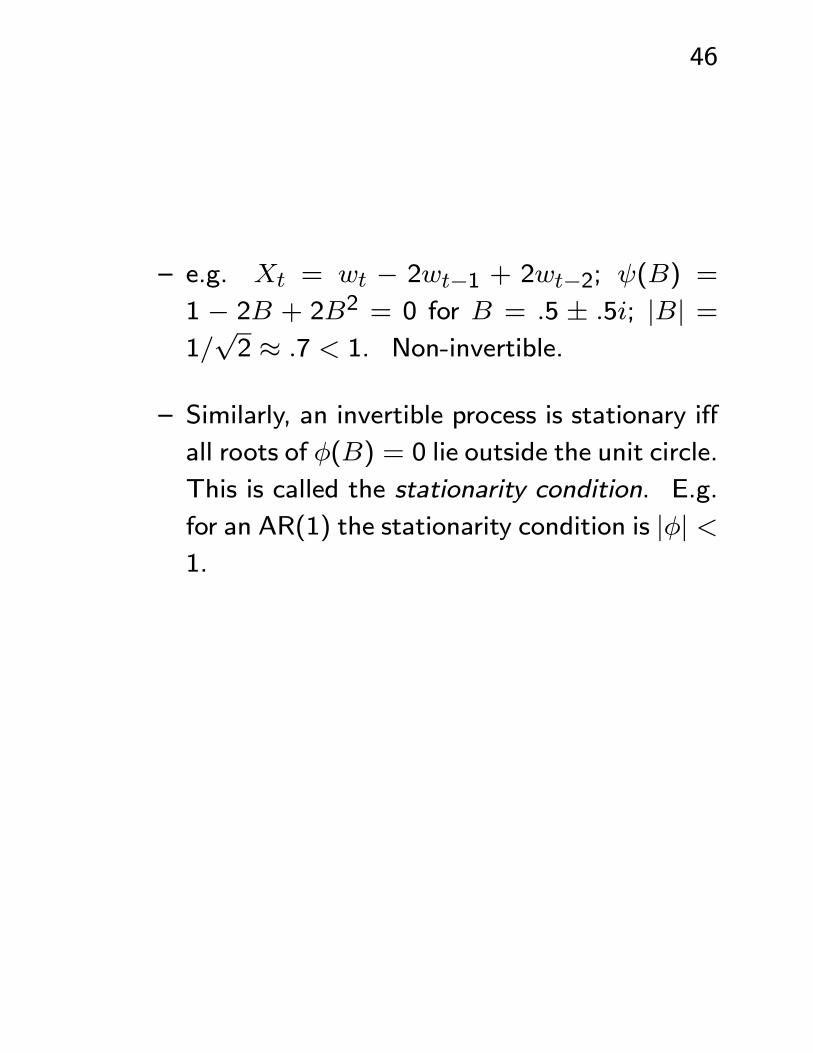
— e.g. Xt = wt − 2wt−1 + 2wt−2; ψ(B) =1 − 2B + 2B2 = 0 for B = .5 ± .5i; |B| =1/√2 ≈ .7 < 1. Non-invertible.

— Similarly, an invertible process is stationary iff

all roots of φ(B) = 0 lie outside the unit circle.

This is called the stationarity condition. E.g.

for an AR(1) the stationarity condition is |φ| <1.

47

6. Lecture 6

• Review of previous lecture. Assume now for sim-plicity that the mean is zero:

— Linear process: Xt = ψ(B)wt, ψ(B) = 1 +ψ1B+ψ2B

2+ ... withP∞k=0ψ

2k <∞. Then

γ(m) = σ2w

∞Xk=0

ψkψk+m.

— Linear + “ψk = 0 for k > q”: MA(q) process,γ(m) = 0 for m > q. Characteristic polyno-mial written as

θ(B) = 1− θ1B − θ2B2 − ...− θqB

q.

— Invertible process: φ(B)Xt = wt, φ(B) =1 − φ1B − φ2B

2 − ... withPk |φk| < ∞.

Note this is really Xt; a non-zero mean canbe accommodated as follows:

wt = φ(B)Xt = Xt − φ1Xt−1 − ...

= (Xt − µ)− φ1 (Xt−1 − µ)− ...

= {Xt − φ1Xt−1 − ...}− µ {1− φ1 − φ2 − ...}= φ(B)Xt − α,

48

if α = µφ(1).

— Invertible + “φj = 0 for j > p”: AR(p)

process.

— Wold’s Theorem: Stationary ⇔ Linear.

— A stationary process is invertible iff all roots

of ψ(B) = 0 lie outside the unit circle. Thus

an MA(q) is stationary (linear), not necessarily

invertible.

— An invertible process is stationary iff all roots

of φ(B) = 0 lie outside the unit circle. Thus

an AR(p) is invertible, not necessarily station-

ary.

• Example: MA(2).

Xt = wt − θ1wt−1 − θ2wt−2,θ(B) = 1− θ1B − θ2B

2.

If θ21 +4θ2 < 0 (so both roots are complex), then

invertibility requires |θ2| < 1. Suppose this is

49

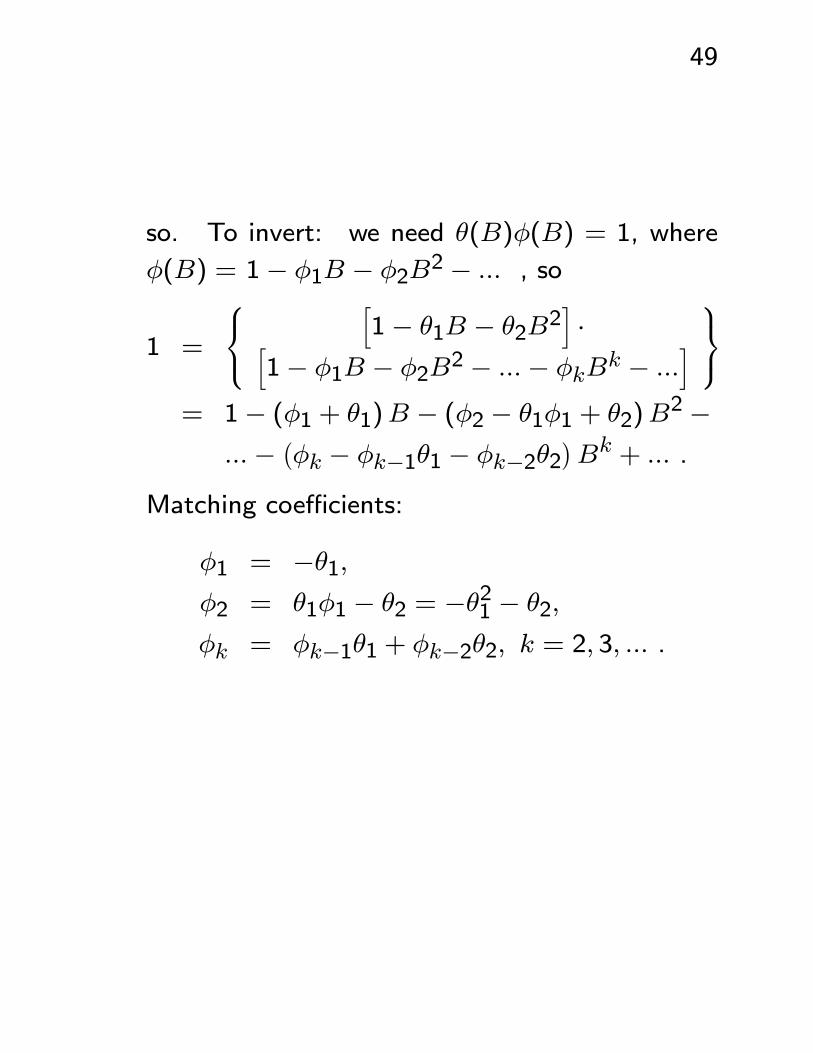
so. To invert: we need θ(B)φ(B) = 1, where

φ(B) = 1− φ1B − φ2B2 − ... , so

1 =

⎧⎨⎩h1− θ1B − θ2B

2i·h

1− φ1B − φ2B2 − ...− φkB

k − ...i ⎫⎬⎭

= 1− (φ1 + θ1)B − (φ2 − θ1φ1 + θ2)B2 −

...−¡φk − φk−1θ1 − φk−2θ2

¢Bk + ... .

Matching coefficients:

φ1 = −θ1,φ2 = θ1φ1 − θ2 = −θ21 − θ2,

φk = φk−1θ1 + φk−2θ2, k = 2, 3, ... .

50

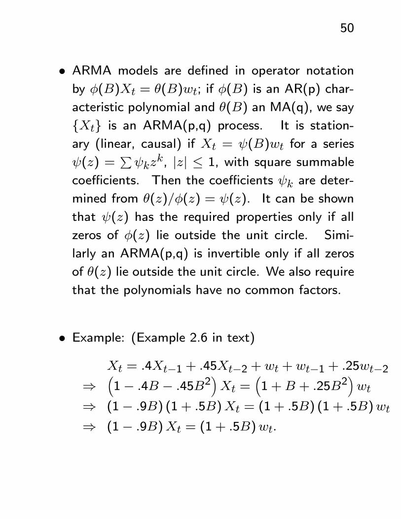
• ARMA models are defined in operator notation

by φ(B)Xt = θ(B)wt; if φ(B) is an AR(p) char-

acteristic polynomial and θ(B) an MA(q), we say

{Xt} is an ARMA(p,q) process. It is station-

ary (linear, causal) if Xt = ψ(B)wt for a series

ψ(z) =Pψkz

k, |z| ≤ 1, with square summable

coefficients. Then the coefficients ψk are deter-

mined from θ(z)/φ(z) = ψ(z). It can be shown

that ψ(z) has the required properties only if all

zeros of φ(z) lie outside the unit circle. Simi-

larly an ARMA(p,q) is invertible only if all zeros

of θ(z) lie outside the unit circle. We also require

that the polynomials have no common factors.

• Example: (Example 2.6 in text)

Xt = .4Xt−1 + .45Xt−2 +wt +wt−1 + .25wt−2⇒

³1− .4B − .45B2

´Xt =

³1 +B + .25B2

´wt

⇒ (1− .9B) (1 + .5B)Xt = (1 + .5B) (1 + .5B)wt

⇒ (1− .9B)Xt = (1 + .5B)wt.

51

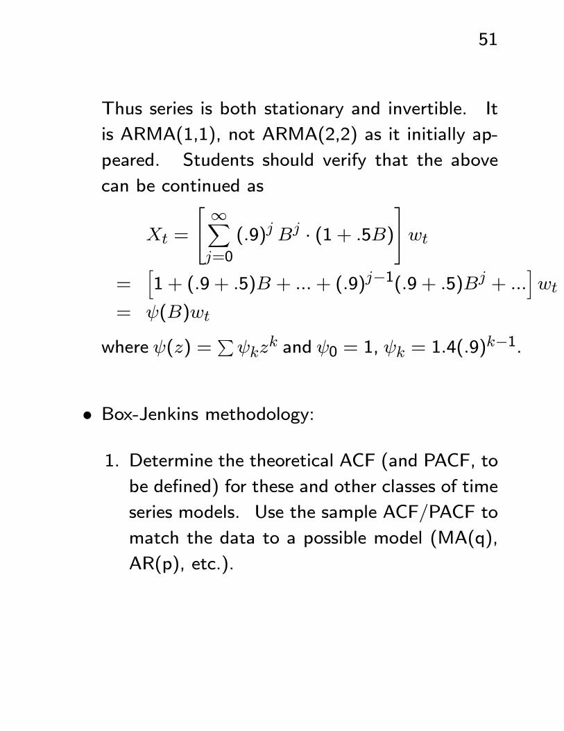
Thus series is both stationary and invertible. It

is ARMA(1,1), not ARMA(2,2) as it initially ap-

peared. Students should verify that the above

can be continued as

Xt =

⎡⎣ ∞Xj=0

(.9)j Bj · (1 + .5B)

⎤⎦wt

=h1 + (.9 + .5)B + ...+ (.9)j−1(.9 + .5)Bj + ...

iwt

= ψ(B)wt

where ψ(z) =Pψkz

k and ψ0 = 1, ψk = 1.4(.9)k−1.

• Box-Jenkins methodology:

1. Determine the theoretical ACF (and PACF, to

be defined) for these and other classes of time

series models. Use the sample ACF/PACF to

match the data to a possible model (MA(q),

AR(p), etc.).

52

2. Estimate parameters using a method appropri-

ate to the chosen model, assess the fit, study

the residuals. The notion of residual will re-

quire a special treatment, for now think of

them as Xt − Xt where, e.g., in an AR(p)

model (Xt = φ1Xt−1+φ2Xt−2+...+φpXt−p+wt) we have Xt = φ1Xt−1 + φ2Xt−2 + ... +

φpXt−p. The residuals should then “look

like” white noise (why?). If the fit is inad-

equate revise steps 1. and 2.

3. Finally use model to forecast.

• We treat these three steps in detail. Recall that

for an MA(q), the autocovariance function is

γ(m) =

(σ2w

Pq−mk=0 θkθk+m, 0 ≤ m ≤ q,0 m > q.

The salient feature is that γ(m) = 0 for m > q;

we look for this in the sample ACF. See Figures

2.1, 2.2.

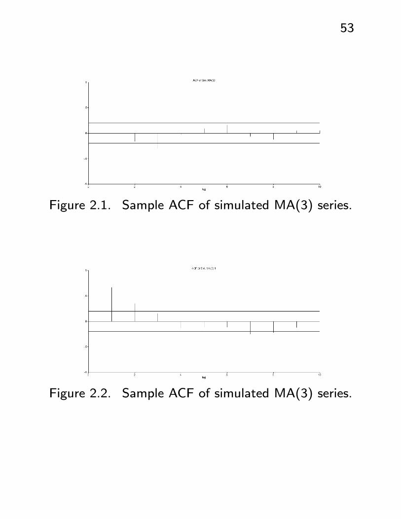
53

Figure 2.1. Sample ACF of simulated MA(3) series.

Figure 2.2. Sample ACF of simulated MA(3) series.

54

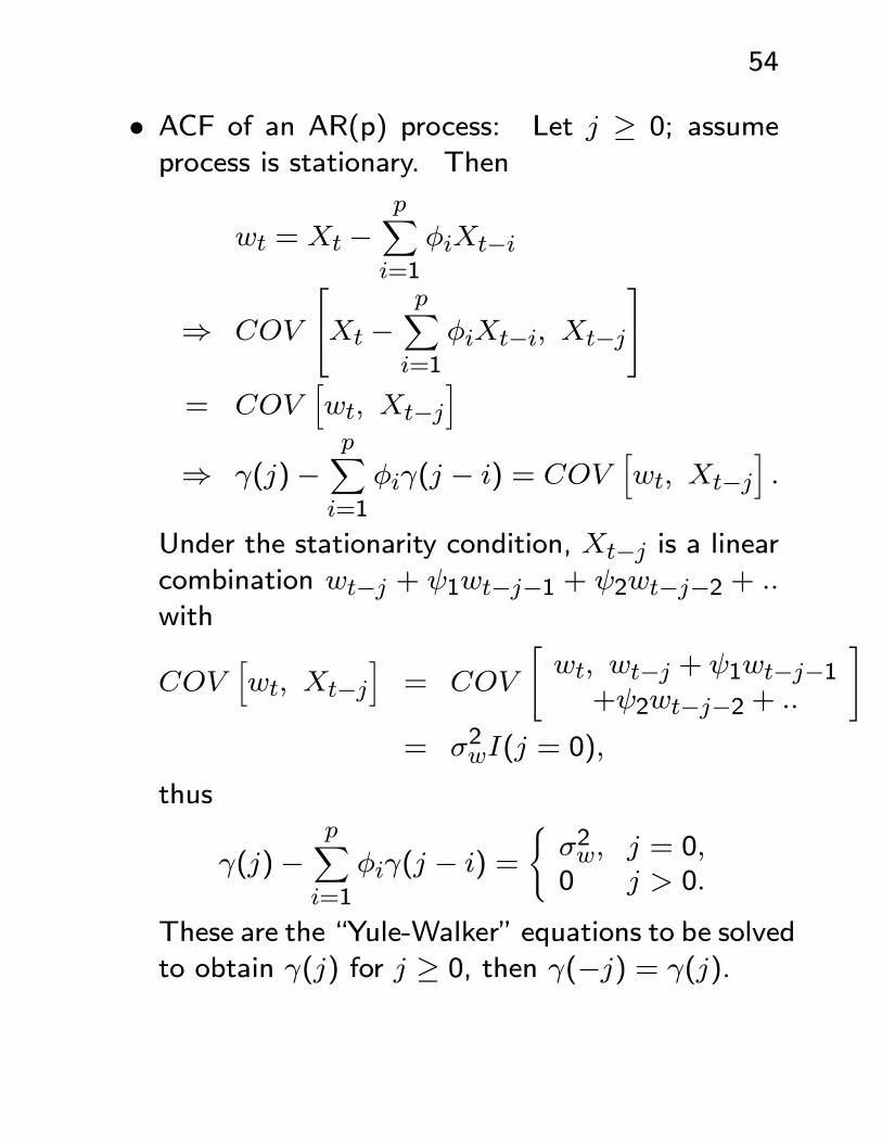
• ACF of an AR(p) process: Let j ≥ 0; assumeprocess is stationary. Then

wt = Xt −pX

i=1

φiXt−i

⇒ COV

⎡⎣Xt −pX

i=1

φiXt−i, Xt−j

⎤⎦= COV

hwt, Xt−j

i⇒ γ(j)−

pXi=1

φiγ(j − i) = COVhwt, Xt−j

i.

Under the stationarity condition, Xt−j is a linearcombination wt−j + ψ1wt−j−1 + ψ2wt−j−2 + ..

with

COVhwt, Xt−j

i= COV

"wt, wt−j + ψ1wt−j−1+ψ2wt−j−2 + ..

#= σ2wI(j = 0),

thus

γ(j)−pX

i=1

φiγ(j − i) =

(σ2w, j = 0,0 j > 0.

These are the “Yule-Walker” equations to be solvedto obtain γ(j) for j ≥ 0, then γ(−j) = γ(j).

55

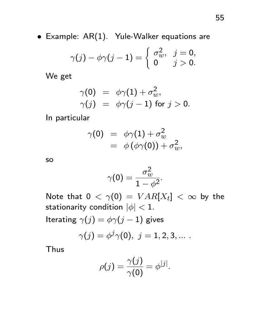
• Example: AR(1). Yule-Walker equations are

γ(j)− φγ(j − 1) =(σ2w, j = 0,0 j > 0.

We get

γ(0) = φγ(1) + σ2w,

γ(j) = φγ(j − 1) for j > 0.

In particular

γ(0) = φγ(1) + σ2w= φ (φγ(0)) + σ2w,

so

γ(0) =σ2w

1− φ2.

Note that 0 < γ(0) = V AR[Xt] < ∞ by the

stationarity condition |φ| < 1.

Iterating γ(j) = φγ(j − 1) gives

γ(j) = φjγ(0), j = 1, 2, 3, ... .

Thus

ρ(j) =γ(j)

γ(0)= φ|j|.

56

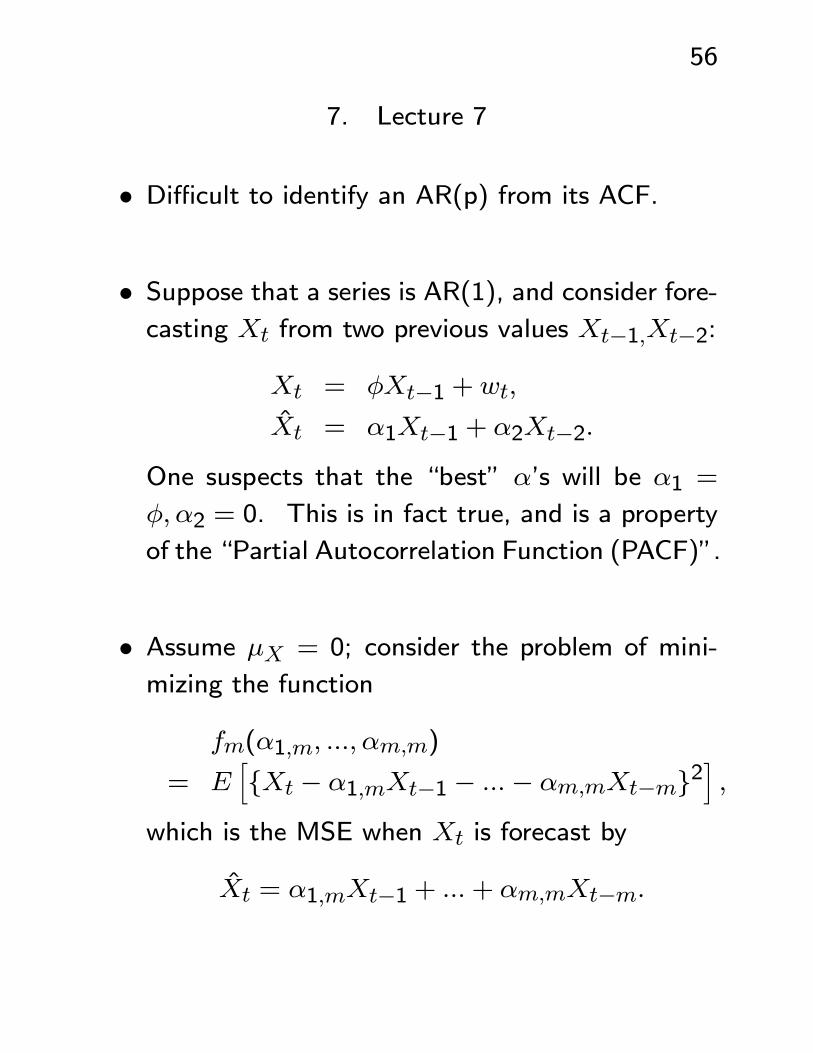
7. Lecture 7

• Difficult to identify an AR(p) from its ACF.

• Suppose that a series is AR(1), and consider fore-casting Xt from two previous values Xt−1,Xt−2:

Xt = φXt−1 +wt,

Xt = α1Xt−1 + α2Xt−2.

One suspects that the “best” α’s will be α1 =

φ, α2 = 0. This is in fact true, and is a property

of the “Partial Autocorrelation Function (PACF)”.

• Assume µX = 0; consider the problem of mini-

mizing the function

fm(α1,m, ..., αm,m)

= Eh{Xt − α1,mXt−1 − ...− αm,mXt−m}2

i,

which is the MSE when Xt is forecast by

Xt = α1,mXt−1 + ...+ αm,mXt−m.

57

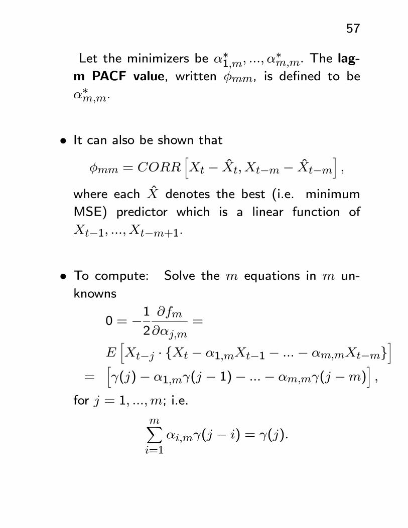
Let the minimizers be α∗1,m, ..., α∗m,m. The lag-

m PACF value, written φmm, is defined to be

α∗m,m.

• It can also be shown that

φmm = CORRhXt − Xt,Xt−m − Xt−m

i,

where each X denotes the best (i.e. minimum

MSE) predictor which is a linear function of

Xt−1, ...,Xt−m+1.

• To compute: Solve the m equations in m un-

knowns

0 = −12

∂fm

∂αj,m=

EhXt−j · {Xt − α1,mXt−1 − ...− αm,mXt−m}

i=

hγ(j)− α1,mγ(j − 1)− ...− αm,mγ(j −m)

i,

for j = 1, ...,m; i.e.

mXi=1

αi,mγ(j − i) = γ(j).

58

Then

m = 1 : φ11 = ρ(1),

m = 2 : φ22 =ρ(2)− ρ2(1)

1− ρ2(1), etc.

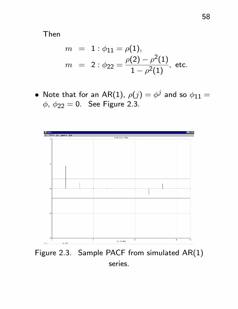
• Note that for an AR(1), ρ(j) = φj and so φ11 =φ, φ22 = 0. See Figure 2.3.

Figure 2.3. Sample PACF from simulated AR(1)

series.

59

• In general, if {Xt} is AR(p) and stationary, thenφpp = φp and φmm = 0 for m > p.

Proof: Write Xt =Ppj=1 φjXt−j + wt, so for

m ≥ p

fm(α1,m, ..., αm,m)

= E

⎡⎢⎣⎧⎨⎩ wt +

Ppj=1

³φj − αj,m

´Xt−j

−Pmj=p+1αj,mXt−j

⎫⎬⎭2⎤⎥⎦

= Eh{wt + Z}2

i, say,

(where Z is uncorrelated with wt - why?),

= σ2w +E[Z2].

This is minimized if Z = 0 with probability 1, i.e.

if αj,m = φj for j ≤ p and = 0 for j > p.

60

• Forecasting. Given r.v.s Xt,Xt−1, ... (into the

infinite past, in principle) we wish to forecast a

future value Xt+l. Let the forecast be Xtt+l.

We will later show that the “best” forecast is

Xtt+l = E

£Xt+l|Xt,Xt−1, ...

¤,

the conditional expected value ofXt+l givenXt =

{Xs}ts=−∞. Our general model identification ap-proach, following Box/Jenkins, is then:

1. Tentatively identify a model, generally by look-

ing at its sample ACF/PACF.

2. Estimate the parameters (generally by the method

of Maximum Likelihood, to be covered later).

This allows us to estimate the forecasts Xtt+l,

which depend on unknown parameters, by sub-

stituting estimates to obtain Xtt+l. We define

the residuals by

wt = Xt − Xt−1t .

61

The (adjusted) MLE of σ2w is typically (inARMA(p, q)

models)

σ2w =1

T − 2p− q

TXt=p+1

w2t .

The T−2p−q in the denominator is the num-ber of residuals used (T−p) minus the numberof ARMA parameters estimated (p+ q).

3. The residuals should “look like” white noise.

We study them, and apply various tests of

whiteness. To the extent that they are not

white, we look for possible alternate models.

4. Iterate; finally use the model to forecast.

62

8. Lecture 8

• Conditional expectation. Example: Randomlychoose a stock from a listing. Y = price in oneweek, X = price in the previous week. To predictY, if we have no information about X then thebest (minimum mse) constant predictor of Y isE[Y ]. (Why? What mathematical problem isbeing formulated and solved here?) However,suppose we also know that X = x. Then wecan improve our forecast, by using the forecastY = E[Y |X = x], the mean price of all stockswhose price in the previous week was x.

• In general, if (X,Y ) are any r.v.s, then E[Y |X =x] is the expected value of Y , when the popula-tion is restricted to those pairs with X = x. Weuse the following facts about conditional expec-tation.

(X,Y ) independent ⇒ E[Y |X = x] = E[Y ],

E[X|X = x] = x,

E[g(X)|X = x] = g(x), and more generally

E[g(X,Y )|X = x] = E[g(x, Y )|X = x].

63

In particular,

E[f(X)g(Y )|X = x] = f(x)E[g(Y )|X = x].

• Assume from now on that white noise is Normally

distributed. The important consequence is that

these terms are now independent, not merely un-

correlated, and so

E [ws|wt,wt−1, ...] =

(ws, s ≤ t,0, s > t.

• Put h(x) = E[Y |X = x]. This is a function of

x; when it is evaluated at the r.v. X we call it

h(X) = E[Y |X]. We have the

Double Expectation Theorem:

E {E[Y |X]} = E[Y ].

The inner expectation is with respect to the

conditional distribution and the outer is with re-

spect to the distribution of X; the theorem can

be stated as E[h(X)] = E[Y ], where h(x) is as

above.

64

— Example: Y = house values, X = location

(neighbourhood) of a house. E[Y ] can be

obtained by averaging within neighbourhoods,

then averaging over neighbourhoods.

• Similarly,

EX

nEY |X [g(X,Y )|X]

o= E [g(X,Y )] .

• Minimum MSE forecasting. Consider forecasting

a r.v. Y (unobservable) using another r.v. X (or

set of r.v.s); e.g. Y = Xt+l, X = Xt. We seek

the function g(X) which minimizes the MSE

MSE(g) = Eh{Y − g(X)}2

i.

The required function is g(X) = E[Y |X] (= h(X)).

65

• Proof: We have to show that for any function g,MSE(g) ≥MSE(h). Write

MSE(g)

= Eh{(Y − h(X)) + (h(X)− g(X))}2

i= E

h{Y − h(X)}2

i+E

h{h(X)− g(X)}2

i+2E [(h(X)− g(X)) · (Y − h(X))] .

We will show that the last term = 0; then we have

MSE(g) =MSE(h)+Eh{h(X)− g(X)}2

iwhich

exceeds MSE(h); equality iff g(X) = h(X) with

probability 1. To establish the claim we evaluate

the expected value in stages:

E [(h(X)− g(X)) · (Y − h(X))]

= EX

nEY |X [(h(X)− g(X)) · (Y − h(X))|X]

o.

The inner expectation is (why?)

(h(X)− g(X) ·EY |X [(Y − h(X))|X]= (h(X)− g(X) ·

nEY |X [Y |X]− h(X)

o= 0.

66

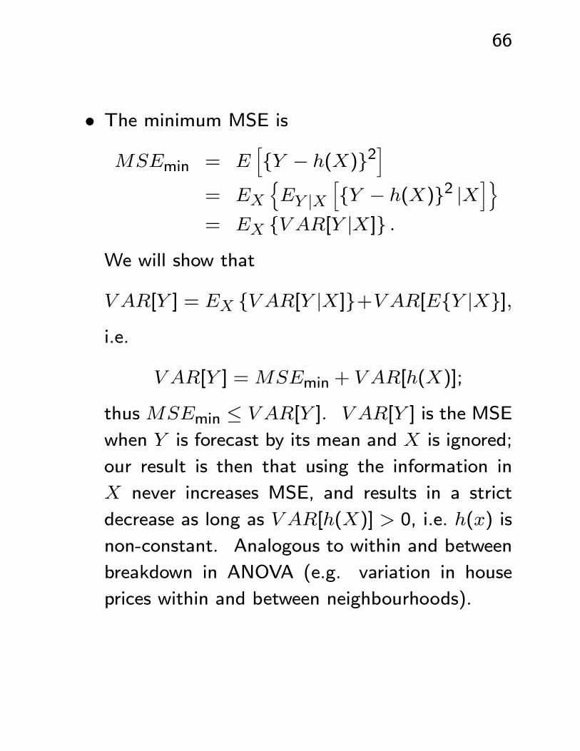
• The minimum MSE is

MSEmin = Eh{Y − h(X)}2

i= EX

nEY |X

h{Y − h(X)}2 |X

io= EX {V AR[Y |X]} .

We will show that

V AR[Y ] = EX {V AR[Y |X]}+V AR[E{Y |X}],

i.e.

V AR[Y ] =MSEmin + V AR[h(X)];

thusMSEmin ≤ V AR[Y ]. V AR[Y ] is the MSE

when Y is forecast by its mean and X is ignored;

our result is then that using the information in

X never increases MSE, and results in a strict

decrease as long as V AR[h(X)] > 0, i.e. h(x) is

non-constant. Analogous to within and between

breakdown in ANOVA (e.g. variation in house

prices within and between neighbourhoods).

67

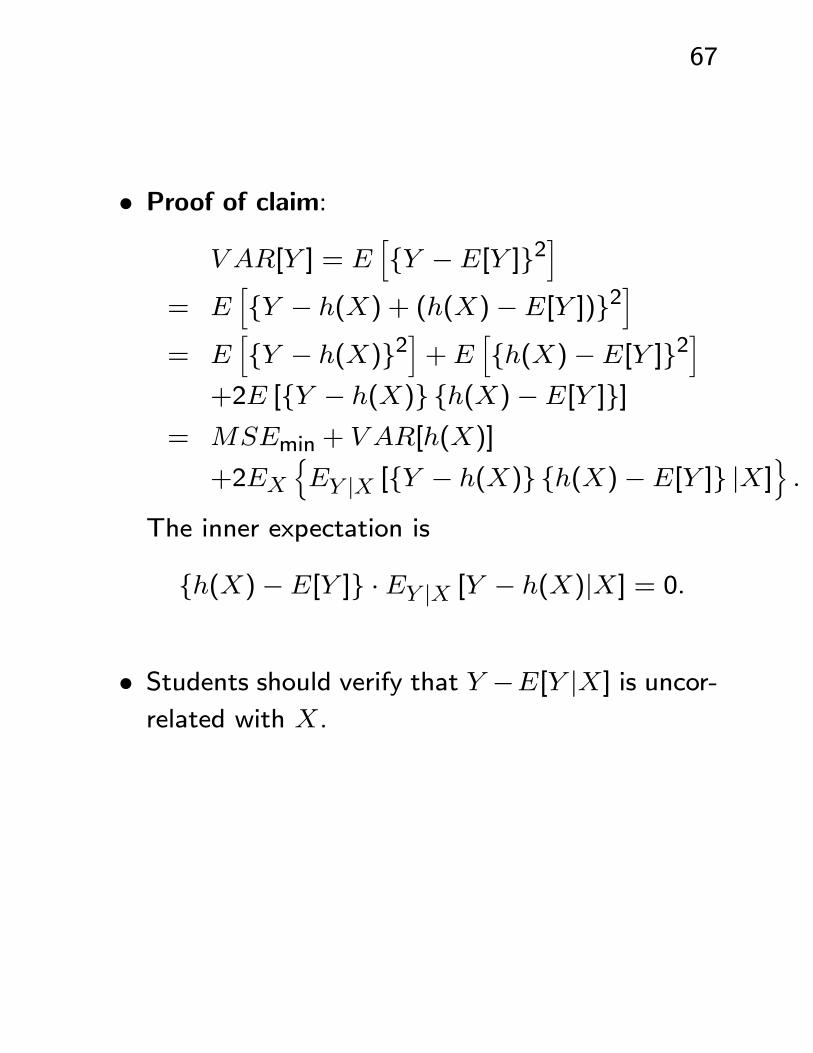
• Proof of claim:

V AR[Y ] = Eh{Y −E[Y ]}2

i= E

h{Y − h(X) + (h(X)−E[Y ])}2

i= E

h{Y − h(X)}2

i+E

h{h(X)−E[Y ]}2

i+2E [{Y − h(X)} {h(X)−E[Y ]}]

= MSEmin + V AR[h(X)]

+2EX

nEY |X [{Y − h(X)} {h(X)−E[Y ]} |X]

o.

The inner expectation is

{h(X)−E[Y ]} ·EY |X [Y − h(X)|X] = 0.

• Students should verify that Y −E[Y |X] is uncor-related with X.

68

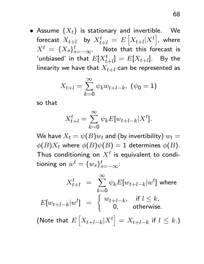
• Assume {Xt} is stationary and invertible. We

forecast Xt+l by Xtt+l = E

hXt+l|Xt

i, where

Xt = {Xs}ts=−∞. Note that this forecast is

‘unbiased’ in that E[Xtt+l] = E[Xt+l]. By the

linearity we have that Xt+l can be represented as

Xt+l =∞Xk=0

ψkwt+l−k, (ψ0 = 1)

so that

Xtt+l =

∞Xk=0

ψkE[wt+l−k|Xt].

We haveXt = ψ(B)wt and (by invertibility) wt =

φ(B)Xt where φ(B)ψ(B) = 1 determines φ(B).

Thus conditioning on Xt is equivalent to condi-

tioning on wt = {ws}ts=−∞:

Xtt+l =

∞Xk=0

ψkE[wt+l−k|wt] where

E[wt+l−k|wt] =

(wt+l−k, if l ≤ k,0, otherwise.

(Note that EhXt+l−k|Xt

i= Xt+l−k if l ≤ k.)

69

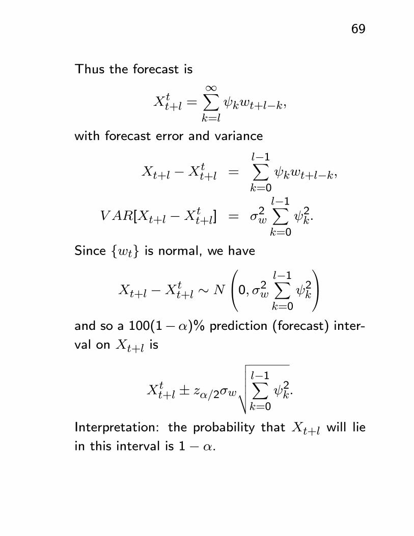
Thus the forecast is

Xtt+l =

∞Xk=l

ψkwt+l−k,

with forecast error and variance

Xt+l −Xtt+l =

l−1Xk=0

ψkwt+l−k,

V AR[Xt+l −Xtt+l] = σ2w

l−1Xk=0

ψ2k.

Since {wt} is normal, we have

Xt+l −Xtt+l ∼ N

⎛⎝0, σ2w l−1Xk=0

ψ2k

⎞⎠and so a 100(1−α)% prediction (forecast) inter-

val on Xt+l is

Xtt+l ± zα/2σw

vuuut l−1Xk=0

ψ2k.

Interpretation: the probability that Xt+l will lie

in this interval is 1− α.

70

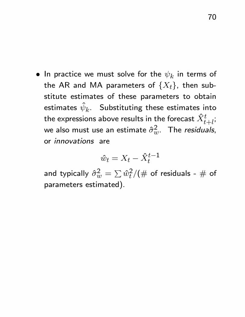
• In practice we must solve for the ψk in terms ofthe AR and MA parameters of {Xt}, then sub-stitute estimates of these parameters to obtain

estimates ψk. Substituting these estimates into

the expressions above results in the forecast Xtt+l;

we also must use an estimate σ2w. The residuals,

or innovations are

wt = Xt − Xt−1t

and typically σ2w =Pw2t /(# of residuals - # of

parameters estimated).

71

9. Lecture 9

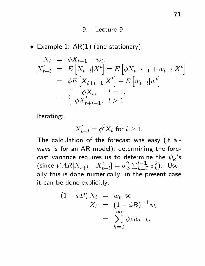
• Example 1: AR(1) (and stationary).

Xt = φXt−1 + wt.

Xtt+l = E

hXt+l|Xt

i= E

hφXt+l−1 +wt+l|Xt

i= φE

hXt+l−1|Xt

i+E

hwt+l|wt

i=

(φXt, l = 1,

φXtt+l−1, l > 1.

Iterating:

Xtt+l = φlXt for l ≥ 1.

The calculation of the forecast was easy (it al-ways is for an AR model); determining the fore-cast variance requires us to determine the ψk’s(since V AR[Xt+l−Xt

t+l] = σ2wPl−1k=0ψ

2k). Usu-

ally this is done numerically; in the present caseit can be done explicitly:

(1− φB)Xt = wt, so

Xt = (1− φB)−1wt

=∞Xk=0

ψkwt−k,

72

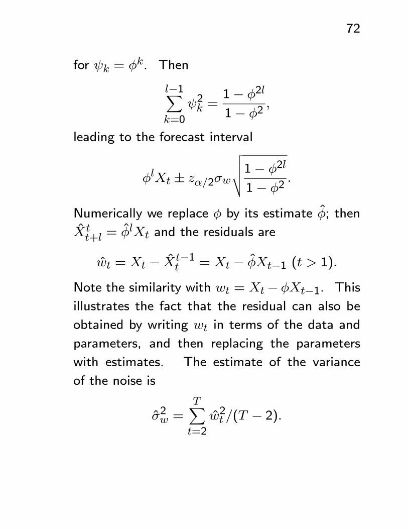
for ψk = φk. Then

l−1Xk=0

ψ2k =1− φ2l

1− φ2,

leading to the forecast interval

φlXt ± zα/2σw

vuut1− φ2l

1− φ2.

Numerically we replace φ by its estimate φ; then

Xtt+l = φlXt and the residuals are

wt = Xt − Xt−1t = Xt − φXt−1 (t > 1).

Note the similarity with wt = Xt−φXt−1. Thisillustrates the fact that the residual can also be

obtained by writing wt in terms of the data and

parameters, and then replacing the parameters

with estimates. The estimate of the variance

of the noise is

σ2w =TXt=2

w2t /(T − 2).

73

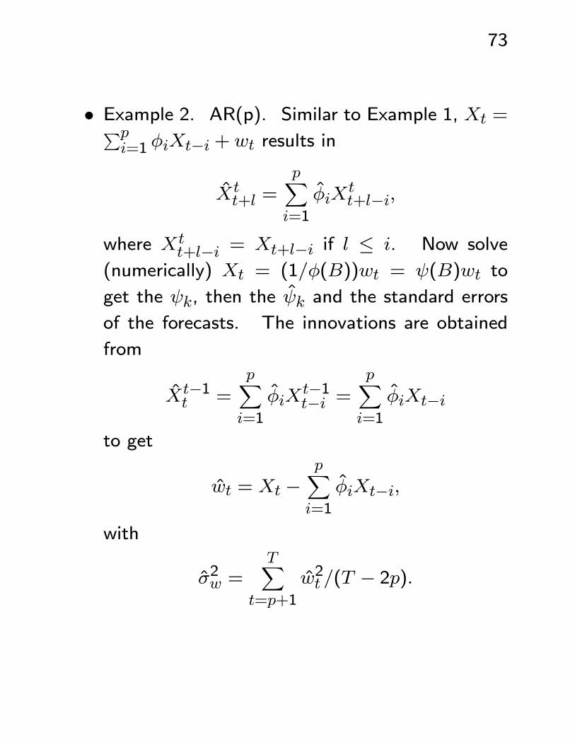
• Example 2. AR(p). Similar to Example 1, Xt =Ppi=1 φiXt−i +wt results in

Xtt+l =

pXi=1

φiXtt+l−i,

where Xtt+l−i = Xt+l−i if l ≤ i. Now solve

(numerically) Xt = (1/φ(B))wt = ψ(B)wt to

get the ψk, then the ψk and the standard errors

of the forecasts. The innovations are obtained

from

Xt−1t =

pXi=1

φiXt−1t−i =

pXi=1

φiXt−i

to get

wt = Xt −pX

i=1

φiXt−i,

with

σ2w =TX

t=p+1

w2t /(T − 2p).

74

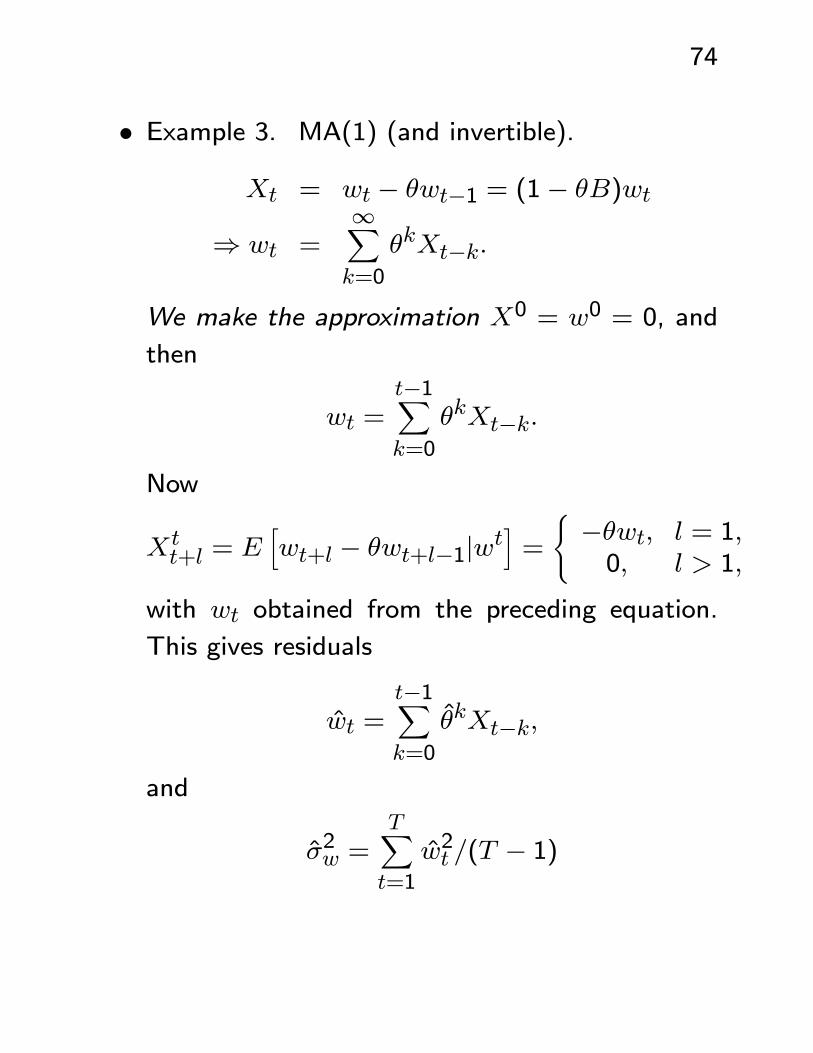
• Example 3. MA(1) (and invertible).

Xt = wt − θwt−1 = (1− θB)wt

⇒ wt =∞Xk=0

θkXt−k.

We make the approximation X0 = w0 = 0, and

then

wt =t−1Xk=0

θkXt−k.

Now

Xtt+l = E

hwt+l − θwt+l−1|wt

i=

(−θwt, l = 1,0, l > 1,

with wt obtained from the preceding equation.

This gives residuals

wt =t−1Xk=0

θkXt−k,

and

σ2w =TXt=1

w2t /(T − 1)

75

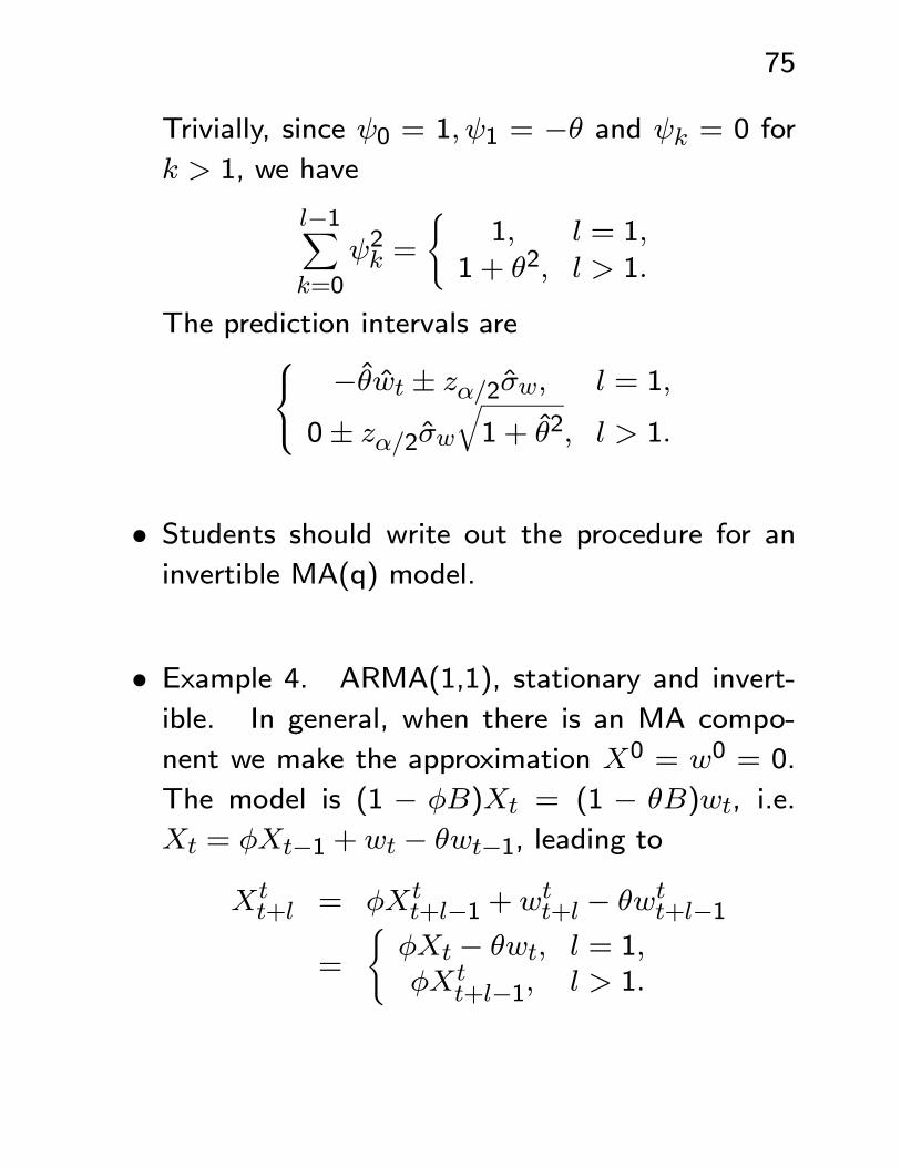
Trivially, since ψ0 = 1, ψ1 = −θ and ψk = 0 for

k > 1, we have

l−1Xk=0

ψ2k =

(1, l = 1,

1 + θ2, l > 1.

The prediction intervals are⎧⎨⎩ −θwt ± zα/2σw, l = 1,

0± zα/2σw

q1 + θ2, l > 1.

• Students should write out the procedure for aninvertible MA(q) model.

• Example 4. ARMA(1,1), stationary and invert-

ible. In general, when there is an MA compo-

nent we make the approximation X0 = w0 = 0.

The model is (1 − φB)Xt = (1 − θB)wt, i.e.

Xt = φXt−1 +wt − θwt−1, leading to

Xtt+l = φXt

t+l−1 +wtt+l − θwt

t+l−1

=

(φXt − θwt, l = 1,φXt

t+l−1, l > 1.

76

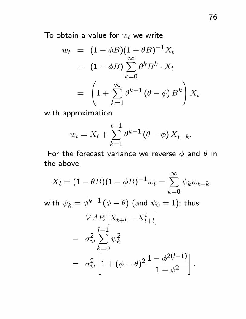
To obtain a value for wt we write

wt = (1− φB)(1− θB)−1Xt

= (1− φB)∞Xk=0

θkBk ·Xt

=

⎛⎝1 + ∞Xk=1

θk−1 (θ − φ)Bk

⎞⎠Xt

with approximation

wt = Xt +t−1Xk=1

θk−1 (θ − φ)Xt−k.

For the forecast variance we reverse φ and θ inthe above:

Xt = (1− θB)(1− φB)−1wt =∞Xk=0

ψkwt−k

with ψk = φk−1 (φ− θ) (and ψ0 = 1); thus

V ARhXt+l −Xt

t+l

i= σ2w

l−1Xk=0

ψ2k

= σ2w

"1 + (φ− θ)2

1− φ2(l−1)

1− φ2

#.

77

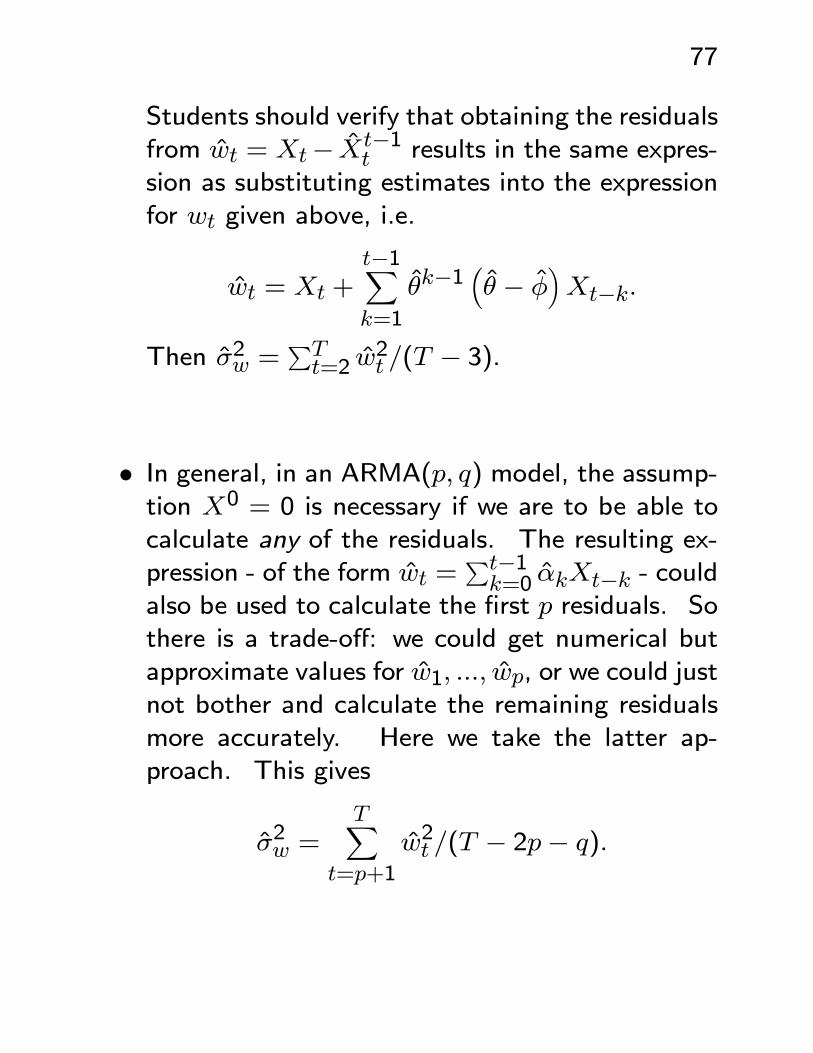
Students should verify that obtaining the residualsfrom wt = Xt− Xt−1

t results in the same expres-sion as substituting estimates into the expressionfor wt given above, i.e.

wt = Xt +t−1Xk=1

θk−1³θ − φ

´Xt−k.

Then σ2w =PTt=2 w

2t /(T − 3).

• In general, in an ARMA(p, q) model, the assump-tion X0 = 0 is necessary if we are to be able tocalculate any of the residuals. The resulting ex-pression - of the form wt =

Pt−1k=0 αkXt−k - could

also be used to calculate the first p residuals. Sothere is a trade-off: we could get numerical butapproximate values for w1, ..., wp, or we could justnot bother and calculate the remaining residualsmore accurately. Here we take the latter ap-proach. This gives

σ2w =TX

t=p+1

w2t /(T − 2p− q).

78

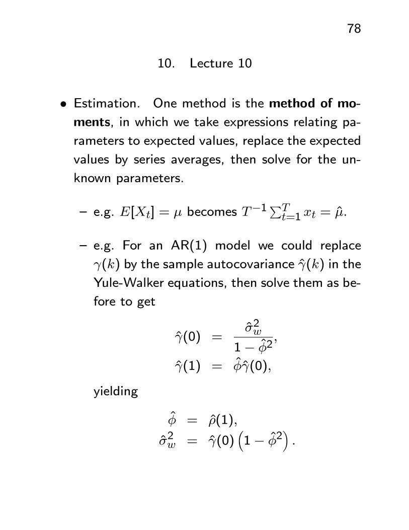
10. Lecture 10

• Estimation. One method is the method of mo-

ments, in which we take expressions relating pa-

rameters to expected values, replace the expected

values by series averages, then solve for the un-

known parameters.

— e.g. E[Xt] = µ becomes T−1PTt=1 xt = µ.

— e.g. For an AR(1) model we could replace

γ(k) by the sample autocovariance γ(k) in the

Yule-Walker equations, then solve them as be-

fore to get

γ(0) =σ2w

1− φ2,

γ(1) = φγ(0),

yielding

φ = ρ(1),

σ2w = γ(0)³1− φ2

´.

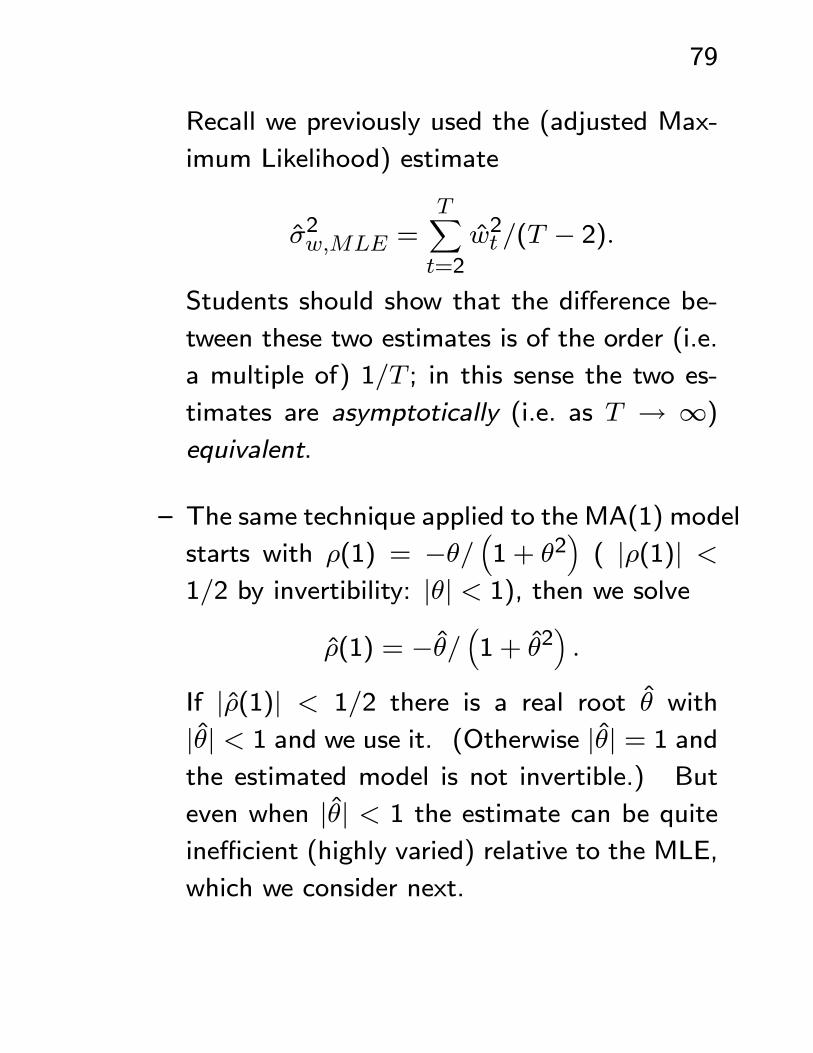
79

Recall we previously used the (adjusted Max-

imum Likelihood) estimate

σ2w,MLE =TXt=2

w2t /(T − 2).

Students should show that the difference be-

tween these two estimates is of the order (i.e.

a multiple of) 1/T ; in this sense the two es-

timates are asymptotically (i.e. as T → ∞)equivalent.

— The same technique applied to the MA(1) model

starts with ρ(1) = −θ/³1 + θ2

´( |ρ(1)| <

1/2 by invertibility: |θ| < 1), then we solve

ρ(1) = −θ/³1 + θ2

´.

If |ρ(1)| < 1/2 there is a real root θ with

|θ| < 1 and we use it. (Otherwise |θ| = 1 andthe estimated model is not invertible.) But

even when |θ| < 1 the estimate can be quite

inefficient (highly varied) relative to the MLE,

which we consider next.

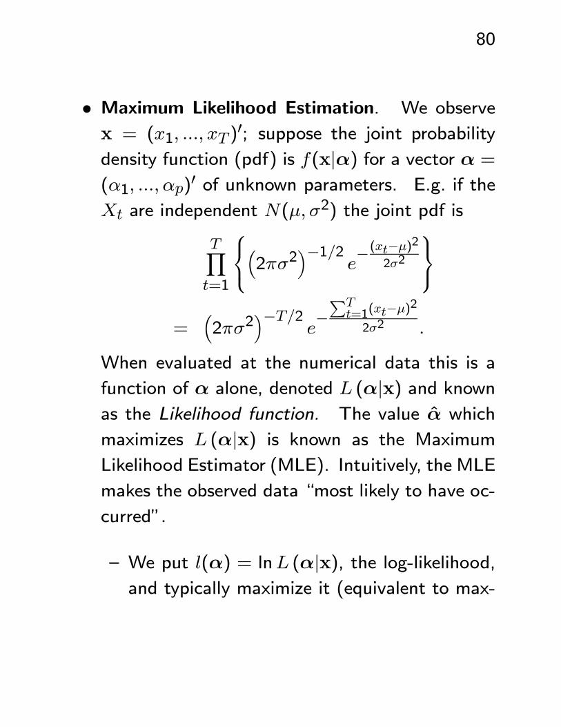
80

• Maximum Likelihood Estimation. We observe

x = (x1, ..., xT )0; suppose the joint probability

density function (pdf) is f(x|α) for a vector α =(α1, ..., αp)

0 of unknown parameters. E.g. if the

Xt are independent N(µ, σ2) the joint pdf is

TYt=1

⎧⎨⎩³2πσ2´−1/2 e−(xt−µ)2

2σ2

⎫⎬⎭=

³2πσ2

´−T/2e−PT

t=1(xt−µ)2

2σ2 .

When evaluated at the numerical data this is a

function of α alone, denoted L (α|x) and knownas the Likelihood function. The value α which

maximizes L (α|x) is known as the MaximumLikelihood Estimator (MLE). Intuitively, the MLE

makes the observed data “most likely to have oc-

curred”.

— We put l(α) = lnL (α|x), the log-likelihood,and typically maximize it (equivalent to max-

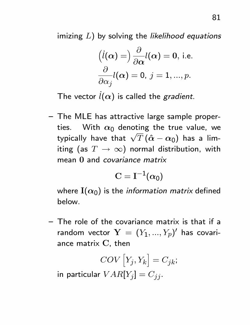
81

imizing L) by solving the likelihood equations³l(α) =

´ ∂

∂αl(α) = 0, i.e.

∂

∂αjl(α) = 0, j = 1, ..., p.

The vector l(α) is called the gradient.

— The MLE has attractive large sample proper-

ties. With α0 denoting the true value, we

typically have that√T (α−α0) has a lim-

iting (as T → ∞) normal distribution, withmean 0 and covariance matrix

C = I−1(α0)

where I(α0) is the information matrix defined

below.

— The role of the covariance matrix is that if a

random vector Y = (Y1, ..., Yp)0 has covari-

ance matrix C, then

COVhYj, Yk

i= Cjk;

in particular V AR[Yj] = Cjj.

82

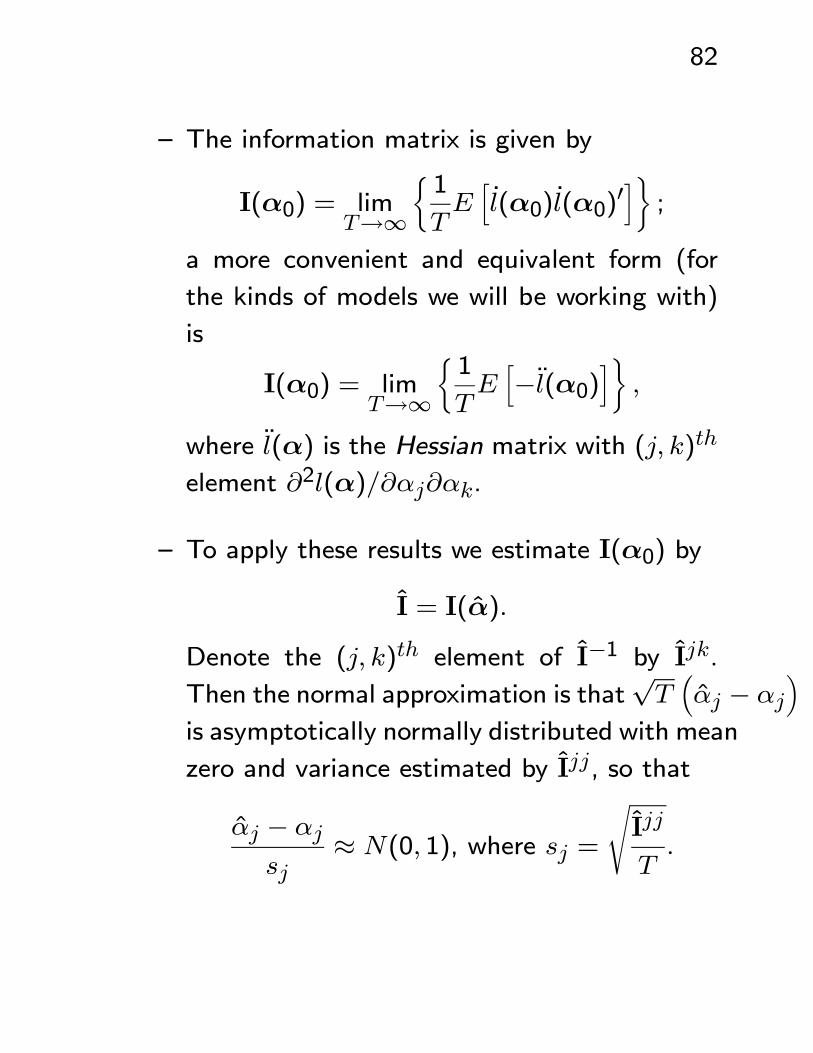
— The information matrix is given by

I(α0) = limT→∞

½1

TEhl(α0)l(α0)

0i¾ ;a more convenient and equivalent form (for

the kinds of models we will be working with)

is

I(α0) = limT→∞

½1

TEh−l(α0)

i¾,

where l(α) is the Hessian matrix with (j, k)th

element ∂2l(α)/∂αj∂αk.

— To apply these results we estimate I(α0) by

I = I(α).

Denote the (j, k)th element of I−1 by Ijk.Then the normal approximation is that

√T³αj − αj

´is asymptotically normally distributed with mean

zero and variance estimated by Ijj, so that

αj − αj

sj≈ N(0, 1), where sj =

sIjj

T.

83

Then, e.g., the p-value for the hypothesis H0 :

αj = 0 against a two-sided alternative is

p = 2P

ÃZ >

¯¯αjsj

¯¯!,

supplied on the ASTSA printout.

• Example 1. AR(1) with a constant: Xt = φ0 +

φ1Xt−1+wt. As is commonly done for AR mod-

els we will carry out an analysis conditional onX1;

i.e. we act as if X1 is not random, but is the con-

stant x1. We can then carry out the following

steps:

1. Write out the pdf of X2, ...,XT .

2. From 1. the log-likelihood is l(α) = lnL (α|x),where α =

³φ0, φ1, σ

2w

´0.

3. Maximize l(α) to obtain the MLEs³φ0, φ1, σ

2w

´.

4. Obtain the information matrix and its esti-

mated inverse.

84

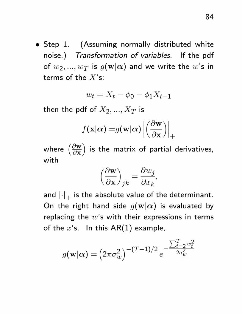
• Step 1. (Assuming normally distributed white

noise.) Transformation of variables. If the pdf

of w2, ..., wT is g(w|α) and we write the w’s interms of the X’s:

wt = Xt − φ0 − φ1Xt−1

then the pdf of X2, ...,XT is

f(x|α) =g(w|α)¯µ∂w

∂x

¶¯+

where³∂w∂x

´is the matrix of partial derivatives,

with µ∂w

∂x

¶jk=

∂wj

∂xk,

and |·|+ is the absolute value of the determinant.On the right hand side g(w|α) is evaluated byreplacing the w’s with their expressions in terms

of the x’s. In this AR(1) example,

g(w|α) =³2πσ2w

´−(T−1)/2e−PT

t=2w2t

2σ2w

85

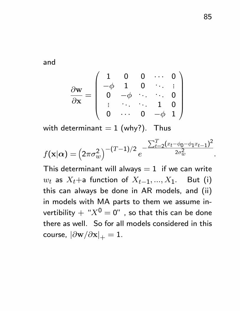
and

∂w

∂x=

⎛⎜⎜⎜⎜⎜⎜⎝1 0 0 · · · 0−φ 1 0 . . . ...0 −φ . . . . . . 0... . . . . . . 1 00 · · · 0 −φ 1

⎞⎟⎟⎟⎟⎟⎟⎠with determinant = 1 (why?). Thus

f(x|α) =³2πσ2w

´−(T−1)/2e−PT

t=2(xt−φ0−φ1xt−1)2

2σ2w .

This determinant will always = 1 if we can write

wt as Xt+a function of Xt−1, ...,X1. But (i)

this can always be done in AR models, and (ii)

in models with MA parts to them we assume in-

vertibility + “X0 = 0” , so that this can be done

there as well. So for all models considered in this

course, |∂w/∂x|+ = 1.

86

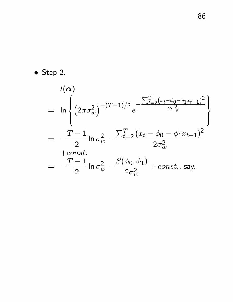
• Step 2.

l(α)

= ln

⎧⎪⎪⎨⎪⎪⎩³2πσ2w

´−(T−1)/2e−PT

t=2(xt−φ0−φ1xt−1)2

2σ2w

⎫⎪⎪⎬⎪⎪⎭= −T − 1

2lnσ2w −

PTt=2 (xt − φ0 − φ1xt−1)

2

2σ2w+const.

= −T − 12

lnσ2w −S(φ0, φ1)

2σ2w+ const., say.

87

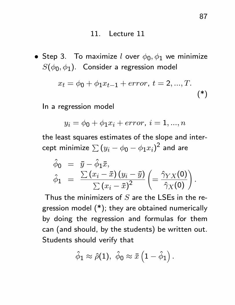
11. Lecture 11

• Step 3. To maximize l over φ0, φ1 we minimize

S(φ0, φ1). Consider a regression model

xt = φ0 + φ1xt−1 + error, t = 2, ..., T.

(*)

In a regression model

yi = φ0 + φ1xi + error, i = 1, ..., n

the least squares estimates of the slope and inter-

cept minimizeP(yi − φ0 − φ1xi)

2 and are

φ0 = y − φ1x,

φ1 =

P(xi − x) (yi − y)P

(xi − x)2

Ã=

γY X(0)

γX(0)

!.

Thus the minimizers of S are the LSEs in the re-

gression model (*); they are obtained numerically

by doing the regression and formulas for them

can (and should, by the students) be written out.

Students should verify that

φ1 ≈ ρ(1), φ0 ≈ x³1− φ1

´.

88

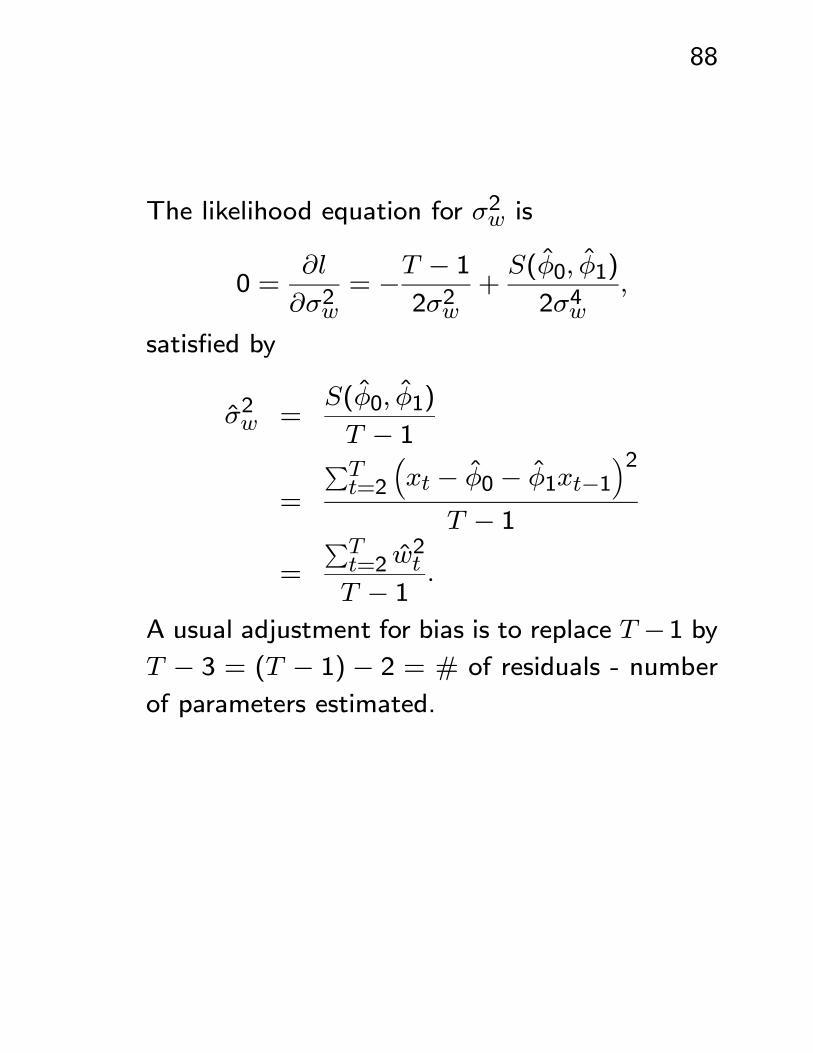
The likelihood equation for σ2w is

0 =∂l

∂σ2w= −T − 1

2σ2w+S(φ0, φ1)

2σ4w,

satisfied by

σ2w =S(φ0, φ1)

T − 1

=

PTt=2

³xt − φ0 − φ1xt−1

´2T − 1

=

PTt=2 w

2t

T − 1.

A usual adjustment for bias is to replace T −1 byT − 3 = (T − 1)− 2 = # of residuals - number

of parameters estimated.

89

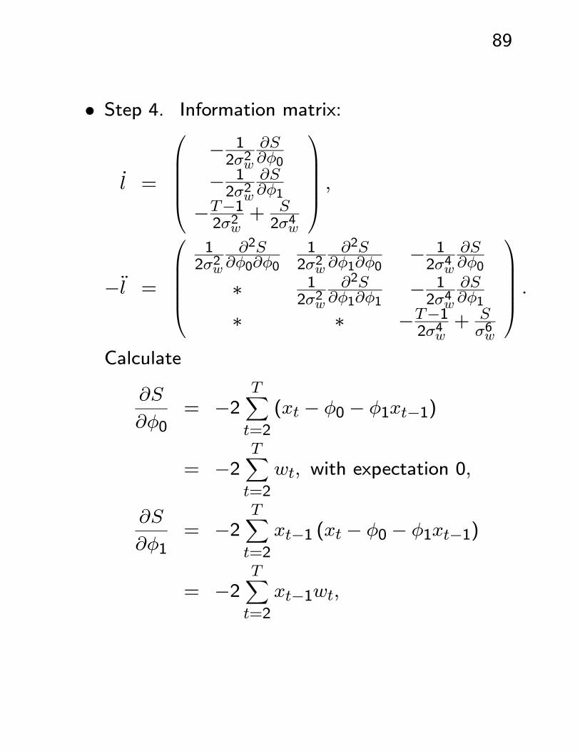
• Step 4. Information matrix:

l =

⎛⎜⎜⎜⎜⎝− 12σ2w

∂S∂φ0

− 12σ2w

∂S∂φ1

−T−12σ2w

+ S2σ4w

⎞⎟⎟⎟⎟⎠ ,

−l =

⎛⎜⎜⎜⎜⎝12σ2w

∂2S∂φ0∂φ0

12σ2w

∂2S∂φ1∂φ0

− 12σ4w

∂S∂φ0

∗ 12σ2w

∂2S∂φ1∂φ1

− 12σ4w

∂S∂φ1

∗ ∗ −T−12σ4w

+ Sσ6w

⎞⎟⎟⎟⎟⎠ .

Calculate

∂S

∂φ0= −2

TXt=2

(xt − φ0 − φ1xt−1)

= −2TXt=2

wt, with expectation 0,

∂S

∂φ1= −2

TXt=2

xt−1 (xt − φ0 − φ1xt−1)

= −2TXt=2

xt−1wt,

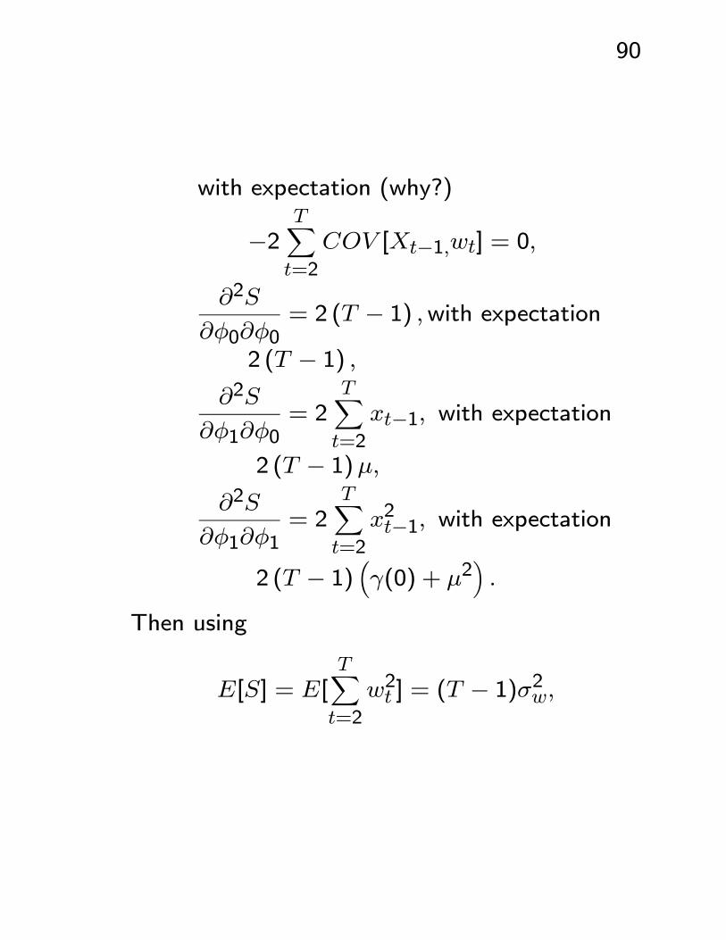
90

with expectation (why?)

−2TXt=2

COV [Xt−1,wt] = 0,

∂2S

∂φ0∂φ0= 2 (T − 1) ,with expectation

2 (T − 1) ,∂2S

∂φ1∂φ0= 2

TXt=2

xt−1, with expectation

2 (T − 1)µ,∂2S

∂φ1∂φ1= 2

TXt=2

x2t−1, with expectation

2 (T − 1)³γ(0) + µ2

´.

Then using

E[S] = E[TXt=2

w2t ] = (T − 1)σ2w,

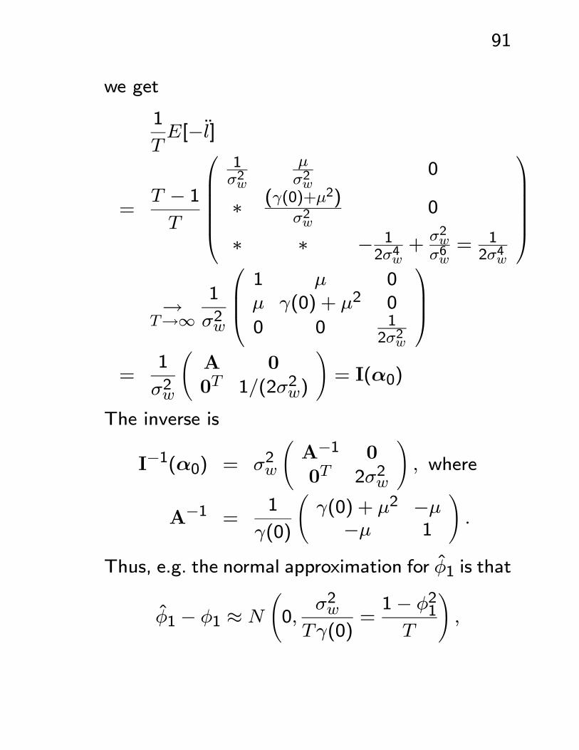
91

we get

1

TE[−l]

=T − 1T

⎛⎜⎜⎜⎜⎜⎝1σ2w

µσ2w

0

∗ (γ(0)+µ2)σ2w

0

∗ ∗ − 12σ4w

+ σ2wσ6w= 12σ4w

⎞⎟⎟⎟⎟⎟⎠

→T→∞

1

σ2w

⎛⎜⎜⎝1 µ 0µ γ(0) + µ2 0

0 0 12σ2w

⎞⎟⎟⎠=

1

σ2w

ÃA 00T 1/(2σ2w)

!= I(α0)

The inverse is

I−1(α0) = σ2w

ÃA−1 00T 2σ2w

!, where

A−1 =1

γ(0)

Ãγ(0) + µ2 −µ−µ 1

!.

Thus, e.g. the normal approximation for φ1 is that

φ1 − φ1 ≈ N

Ã0,

σ2wTγ(0)

=1− φ21T

!,

92

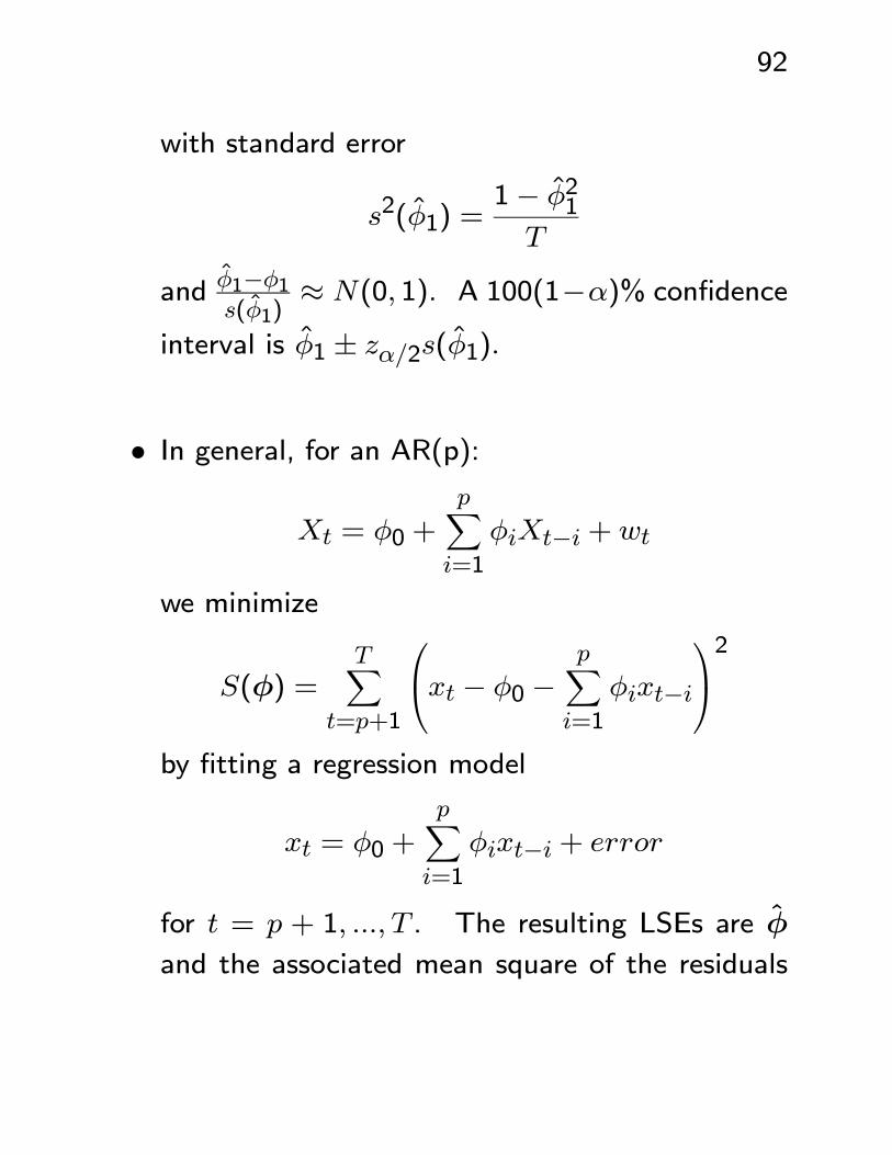
with standard error

s2(φ1) =1− φ21T

and φ1−φ1s(φ1)

≈ N(0, 1). A 100(1−α)% confidence

interval is φ1 ± zα/2s(φ1).

• In general, for an AR(p):

Xt = φ0 +pX

i=1

φiXt−i +wt

we minimize

S(φ) =TX

t=p+1

⎛⎝xt − φ0 −pX

i=1

φixt−i

⎞⎠2

by fitting a regression model

xt = φ0 +pX

i=1

φixt−i + error

for t = p + 1, ..., T . The resulting LSEs are φ

and the associated mean square of the residuals

93

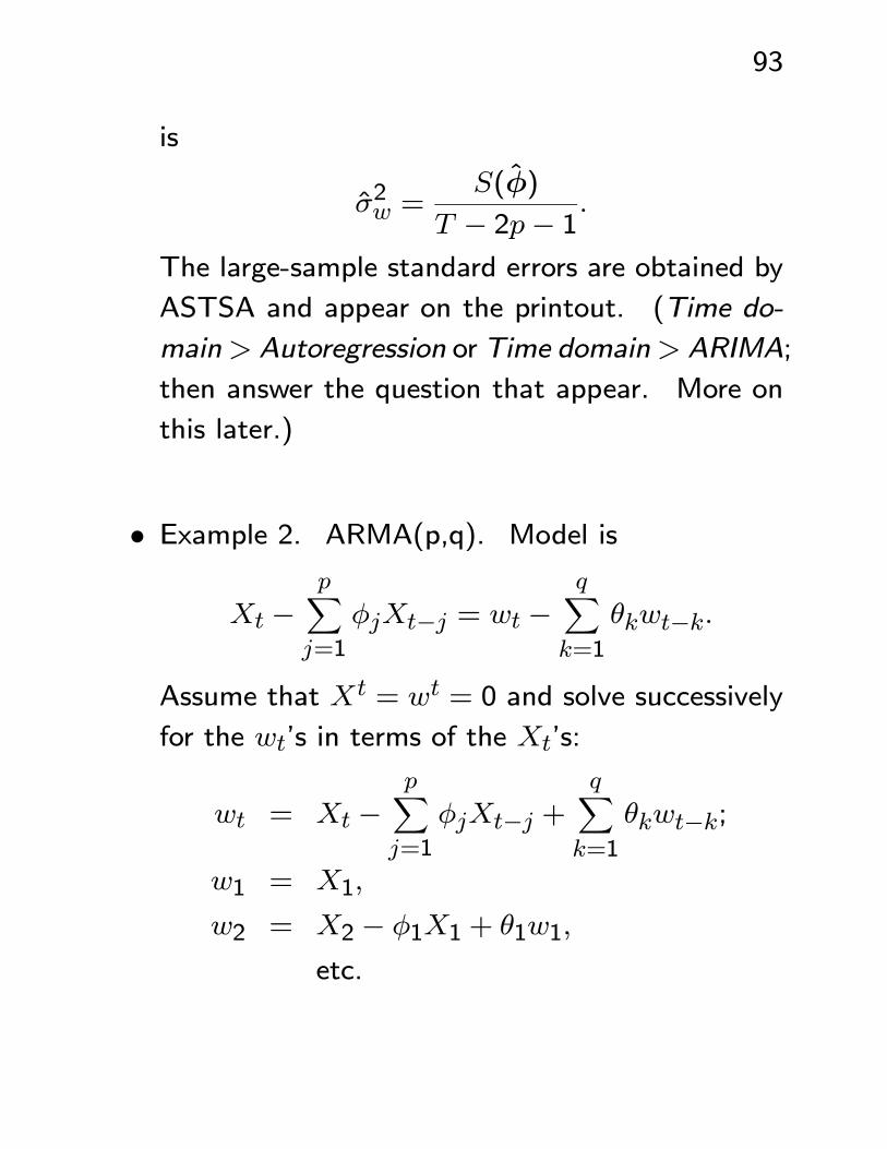
is

σ2w =S(φ)

T − 2p− 1.

The large-sample standard errors are obtained by

ASTSA and appear on the printout. (Time do-

main> Autoregression or Time domain> ARIMA;

then answer the question that appear. More on

this later.)

• Example 2. ARMA(p,q). Model is

Xt −pX

j=1

φjXt−j = wt −qX

k=1

θkwt−k.

Assume that Xt = wt = 0 and solve successively

for the wt’s in terms of the Xt’s:

wt = Xt −pX

j=1

φjXt−j +qX

k=1

θkwt−k;

w1 = X1,

w2 = X2 − φ1X1 + θ1w1,

etc.

94

In this way we write³wp+1, ..., wT

´in terms of³

xp+1, ..., xT´. The Jacobian is again = 1 and

so

f(x|α) =³2πσ2w

´−(T−p)/2e−S(φ,θ)

2σ2w ,

where S(φ,θ) =PTt=p+1w

2t (φ,θ). (It is usual

to omit the first p wt’s, since they are based

on so little data and on the assumption men-

tioned above. Equivalently we are conditioning

on them.) Now S(φ, θ) is minimized numeri-

cally to obtain the MLEs φ, θ. The MLE of σ2wis obtained from the likelihood equation and is

S(φ, θ)/(T − p); it is often adjusted for bias to

give

σ2w =S(φ, θ)

T − 2p− q.

95

• The matrix

I(α0) = limT→∞

½1

TEh−l(α0)

i¾is sometimes estimated by the “observed infor-mation matrix” 1

T

³−l(α)

´evaluated at the data

{xt}. This is numerically simpler.

• Students should write out the procedure for anMA(1) model.

• The numerical calculations also rely on a modifi-cation of least squares regression. Gauss-Newtonalgorithm: We are to minimize

S(ψ) =Xt

w2t (ψ),

where ψ is a p-dimensional vector of parameters.The idea is to set up a series of least squares re-gressions converging to the solution. First choosean initial value ψ0. (ASTSA will put all compo-nents = .1 if “.1 guess” is chosen. Otherwise,it will compute method of moments estimates,by equating the theoretical and sample ACF andPACF values. This takes longer.)

96

• Now expand wt(ψ) around ψ0 by the Mean Value

Theorem:

wt(ψ) ≈ wt(ψ0) + w0t(ψ0) (ψ −ψ0) (1)

= “yt − z0tβ”,

where yt = wt(ψ0), zt = −wt(ψ0), β = ψ −ψ0.

Now

S(ψ) ≈Xt

³yt − z0tβ

´2is minimized by regressing {yt} on {zt} to get theLSE β1. We now set

ψ1 = β1 +ψ0,

expand around ψ1 (i.e. replace ψ0 by ψ1 in (1)),

obtain a revised estimate β2. Iterate to conver-

gence.

97

12. Lecture 12

• A class of nonstationary models is obtained by

taking differences, and assuming that the differ-

enced series is ARMA(p,q):

∇Xt = Xt −Xt−1 = (1−B)Xt,

∇2Xt = ∇(∇Xt) = (1−B)2Xt,

etc.

We say {Xt} is ARIMA(p,d,q) (“Integrated ARMA”)if ∇dXt is ARMA(p,q). If so,

φ(B)(1−B)dXt = θ(B)wt

for an AR(p) polynomial φ(B) and an MA(q)

polynomial θ(B). Since φ(B)(1−B)d has roots

on the unit circle, {Xt} cannot be stationary.The differenced series

n∇dXt

ois the one we an-

alyze.

98

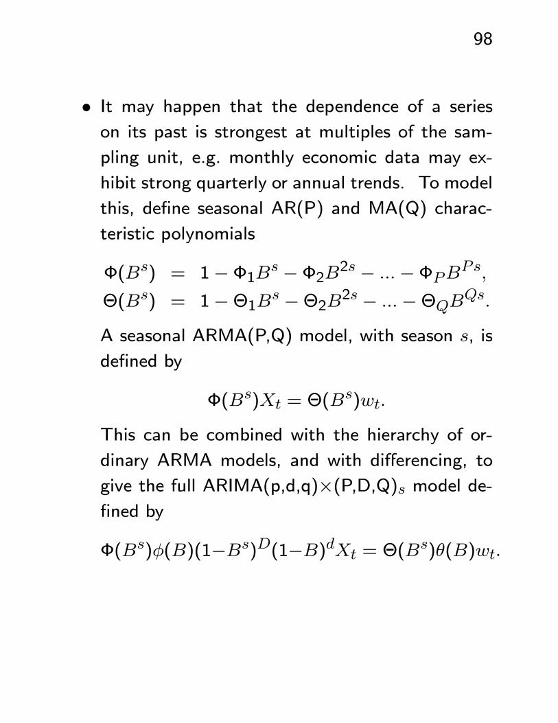
• It may happen that the dependence of a serieson its past is strongest at multiples of the sam-

pling unit, e.g. monthly economic data may ex-

hibit strong quarterly or annual trends. To model

this, define seasonal AR(P) and MA(Q) charac-

teristic polynomials

Φ(Bs) = 1−Φ1Bs − Φ2B

2s − ...−ΦPBPs,

Θ(Bs) = 1−Θ1Bs −Θ2B

2s − ...−ΘQBQs.

A seasonal ARMA(P,Q) model, with season s, is

defined by

Φ(Bs)Xt = Θ(Bs)wt.

This can be combined with the hierarchy of or-

dinary ARMA models, and with differencing, to

give the full ARIMA(p,d,q)×(P,D,Q)s model de-fined by

Φ(Bs)φ(B)(1−Bs)D(1−B)dXt = Θ(Bs)θ(B)wt.

99

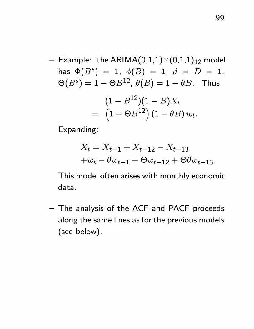
— Example: the ARIMA(0,1,1)×(0,1,1)12 modelhas Φ(Bs) = 1, φ(B) = 1, d = D = 1,

Θ(Bs) = 1−ΘB12, θ(B) = 1− θB. Thus

(1−B12)(1−B)Xt

=³1−ΘB12

´(1− θB)wt.

Expanding:

Xt = Xt−1 +Xt−12 −Xt−13+wt − θwt−1 −Θwt−12 +Θθwt−13.

This model often arises with monthly economic

data.

— The analysis of the ACF and PACF proceeds

along the same lines as for the previous models

(see below).

100

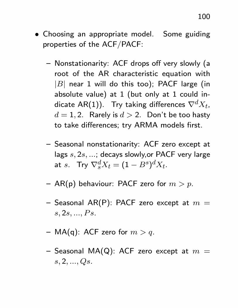
• Choosing an appropriate model. Some guiding

properties of the ACF/PACF:

— Nonstationarity: ACF drops off very slowly (a

root of the AR characteristic equation with

|B| near 1 will do this too); PACF large (inabsolute value) at 1 (but only at 1 could in-

dicate AR(1)). Try taking differences ∇dXt,

d = 1, 2. Rarely is d > 2. Don’t be too hasty

to take differences; try ARMA models first.

— Seasonal nonstationarity: ACF zero except at

lags s, 2s, ...; decays slowly,or PACF very large

at s. Try ∇dsXt = (1−Bs)dXt.

— AR(p) behaviour: PACF zero for m > p.

— Seasonal AR(P): PACF zero except at m =

s, 2s, ..., Ps.

— MA(q): ACF zero for m > q.

— Seasonal MA(Q): ACF zero except at m =

s, 2, ..., Qs.

101

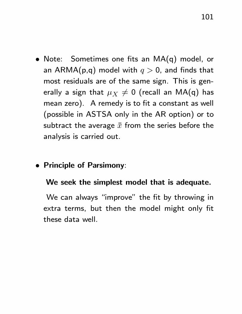
• Note: Sometimes one fits an MA(q) model, or

an ARMA(p,q) model with q > 0, and finds that

most residuals are of the same sign. This is gen-

erally a sign that µX 6= 0 (recall an MA(q) has

mean zero). A remedy is to fit a constant as well

(possible in ASTSA only in the AR option) or to

subtract the average x from the series before the

analysis is carried out.

• Principle of Parsimony:

We seek the simplest model that is adequate.

We can always “improve” the fit by throwing in

extra terms, but then the model might only fit

these data well.

102

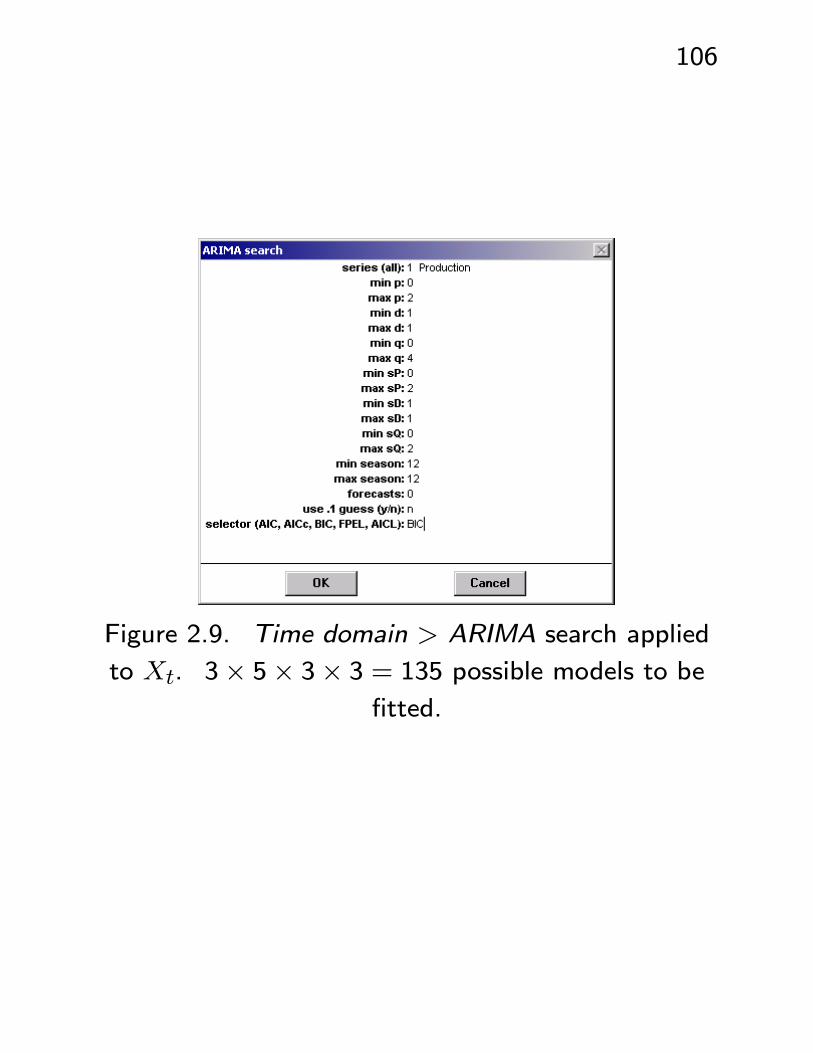
• See Figures 2.4 - 2.11. Example: U.S. Federal

Reserve Board Production Index - an index of eco-

nomic productivity. Plots of data and ACF/PACF

clearly indicate nonstationarity. ACF of ∇Xt in-

dicates seasonal (s = 12) nonstationarity. ACF

and PACF of ∇12∇Xt shows possible models

ARIMA(p = 1− 2, d = 1, q = 1− 4)×(P = 2,D = 1, Q = 1)s=12.

The ARIMA Search facility, using BIC, picks out

ARIMA(1, 1, 0)× (0, 1, 1)12. Note q = P = 0;

the other AR and MA features seem to have ac-

counted for the seeming MA and seasonal AR(2)

behaviour.

103

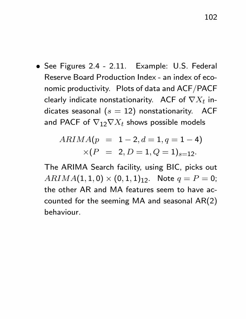
Figure 2.4. U.S. Federal Reserve Board Production

Index (frb.asd in ASTSA). Non-stationarity of mean

is obvious.

104

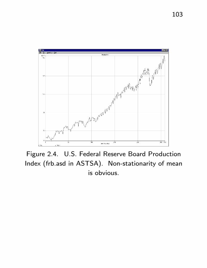
Figure 2.5. ACF decays slowly, PACF spikes at

m = 1. Both indicate nonstationarity.

Figure 2.6. ∇Xt; nonstationary variance exhibited.

105

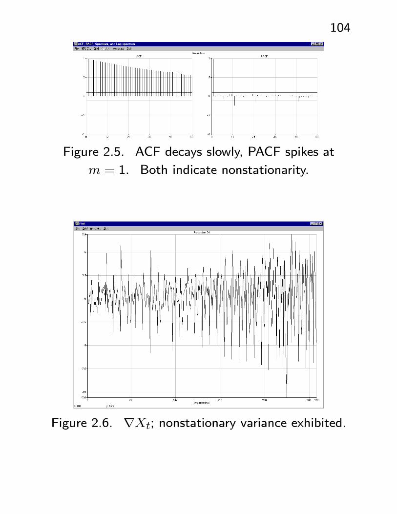
Figure 2.7. ∇Xt; ACF shows seasonal

nonstationarity.

Figure 2.8. ∇12∇Xt. Peak in ACF at m = 12

indicates seasonal (s = 12) MA(1). PACF indicates

AR(1) or AR(2) and (possibly) seasonal AR(2).

106

Figure 2.9. Time domain > ARIMA search applied

to Xt. 3× 5× 3× 3 = 135 possible models to befitted.

107

Figure 2.10. ARIMA search with BIC criterion picks

out ARIMA(1,1,0)×(0,1,1)12. The (default) AICccriterion picks out ARIMA(0,1,4)×(2,1,1)12. One

could argue for either one.

108

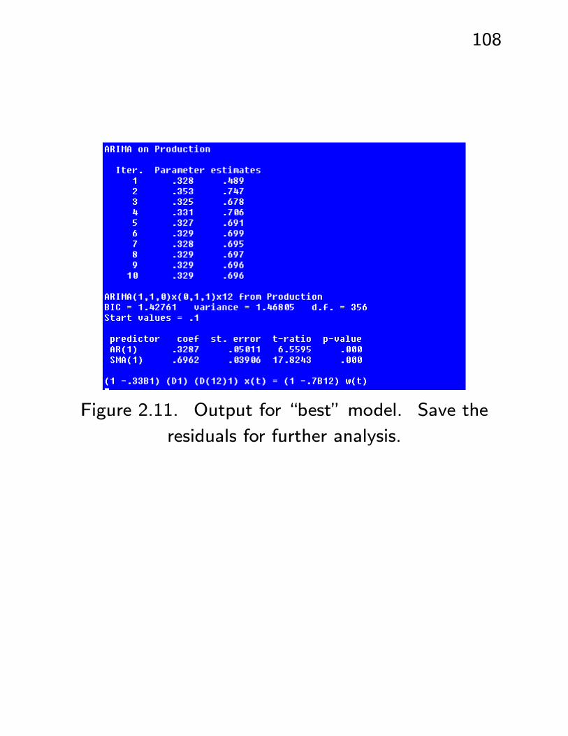
Figure 2.11. Output for “best” model. Save the

residuals for further analysis.

109

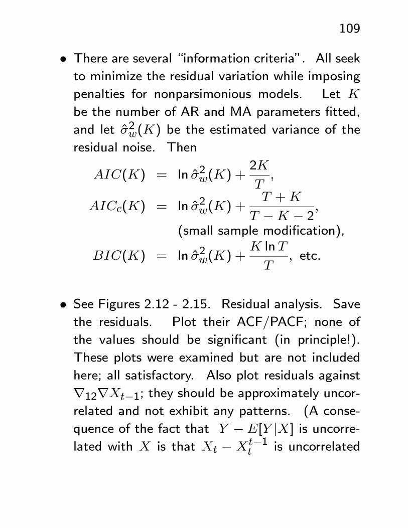
• There are several “information criteria”. All seekto minimize the residual variation while imposing

penalties for nonparsimonious models. Let K

be the number of AR and MA parameters fitted,

and let σ2w(K) be the estimated variance of the

residual noise. Then

AIC(K) = ln σ2w(K) +2K

T,

AICc(K) = ln σ2w(K) +T +K

T −K − 2,

(small sample modification),

BIC(K) = ln σ2w(K) +K lnT

T, etc.

• See Figures 2.12 - 2.15. Residual analysis. Savethe residuals. Plot their ACF/PACF; none of

the values should be significant (in principle!).

These plots were examined but are not included

here; all satisfactory. Also plot residuals against

∇12∇Xt−1; they should be approximately uncor-related and not exhibit any patterns. (A conse-

quence of the fact that Y −E[Y |X] is uncorre-lated with X is that Xt − Xt−1

t is uncorrelated

110

with Xs for s < t, i.e. except for the fact that

the residuals use estimated parameters, they are

uncorrelated with the predictors. This assumes

stationarity, so here we use the differenced series.)

Click on Graph > Residual tests.

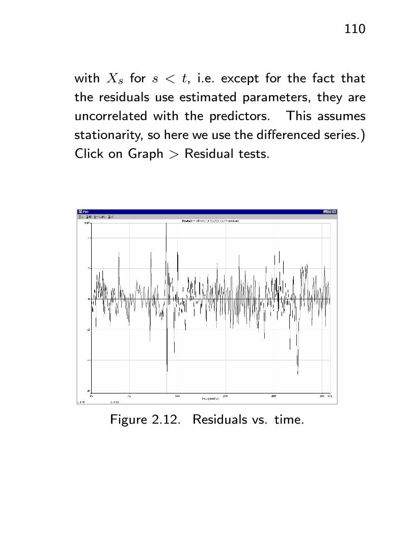
Figure 2.12. Residuals vs. time.

111

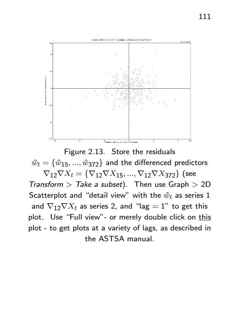
Figure 2.13. Store the residuals

wt = {w15, ..., w372} and the differenced predictors∇12∇Xt = {∇12∇X15, ...,∇12∇X372} (see

Transform > Take a subset). Then use Graph > 2D

Scatterplot and “detail view” with the wt as series 1

and ∇12∇Xt as series 2, and “lag = 1” to get this

plot. Use “Full view”- or merely double click on this

plot - to get plots at a variety of lags, as described in

the ASTSA manual.

112

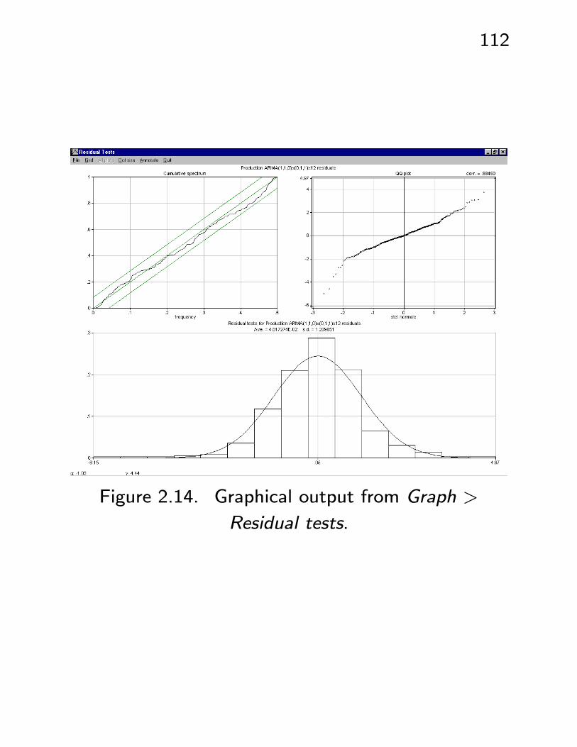
Figure 2.14. Graphical output from Graph >

Residual tests.

113

Figure 2.15. Printed output from Graph > Residual

tests.

114

• Cumulative spectrum test. We will see later

that if the residuals {wt} are white noise, thentheir “spectrum” f(ν) is constantly equal to the

variance, i.e. is ‘flat’. Then the integrated, or

cumulative spectrum, is linear with slope = vari-

ance; here it is divided by σ2w/2 and so should

be linear with a slope of 2. Accounting for ran-

dom variation, it should at least remain in a band

around a straight line through the origin, with a

slope of 2. The graphical output confirms this

and the printed output gives a non-significant p-

value to the hypothesis of a flat spectrum.

115

13. Lecture 13

• Box-Pierce test. Under the hypothesis of white-ness we expect ρw(m) to be small in absolute

value for all m; a test can be based on

Q = T (T + 2)MX

m=1

ρ2w(m)

T −m,

which is approximately ∼ χ2M−K under the null

hypothesis. The p-value is calculated and re-

ported for M −K = 1, 20.

• Fluctuations test (= Runs test). Too few or

too many fluctuations, i.e. changes from an up-

ward trend to a downward trend or vice versa)

constitute evidence against randomness. E.g. an

AR(1) (ρ(1) = φ) with φ near +1 will have few

fluctuations, φ near −1 will result in many.

116

• Normal scores (Q-Q) test. The quantiles of

a distribution F = Fw are the values F−1(q),i.e. the values below which w lies with probability

q. The sample versions are the order statistics

w(1) < w(2) < ... < w(T ): the probability of a

value w falling at or below w(t) is estimated by

t/T , so w(t) can be viewed as the (t/T )th sam-

ple quantile. If the residuals are normal then a

plot of the sample quantiles against the standard

normal quantiles should be linear, with intercept

equal to the mean and slope equal to the standard

deviation (follows from F−1(q) = µ+σΦ−1(q) ifF is the N(µ, σ2) df; students should verify this

identity). The strength of the linearity is mea-

sured by the correlation between the two sets of

quantiles; values too far below 1 lead to rejection

of the hypothesis of normality of the white noise.

117

• The residuals from the more complex model cho-

sen by AICc looked no better.

• A log or square root transformation of the originaldata sometimes improves normality; logging the

data made no difference in this case.

• In contrast, if we fit anARIMA(0, 1, 0)×(0, 1, 1)12,then the ACF/PACF of the residuals clearly shows

the need for the AR(1) component - see Figures

2.16, 2.17. Note also that the largest residual

is now at t = 324 - adding the AR term has ex-

plained the drop at this point to such an extent

that it is now less of a problem than the smaller

drop at t = 128.

118

Figure 2.16. ACF and PACF of residuals from

ARIMA(0, 1, 0)× (0, 1, 1)12 fit.

119

Figure 2.17. Residual tests for

ARIMA(0, 1, 0)× (0, 1, 1)12 fit.

120

Forecasting in the FRB example. Fitted model is

(1− φB)∇∇12Xt =³1−ΘB12

´wt; (1)

this is expanded as

Xt = (1 + φ)Xt−1 − φXt−2 +Xt−12− (1 + φ)Xt−13 + φXt−14 + wt −Θwt−12.(2)

Conditioning on Xt gives

Xtt+l = (1 + φ)Xt

t+l−1 − φXtt+l−2 +Xt

t+l−12− (1 + φ)Xt

t+l−13 + φXtt+l−14 +wt

t+l −Θwtt+l−12.

We consider the case 1 ≤ l ≤ 12 only; l = 13 left as

an exercise. Note that the model is not stationary but

seems to be invertible (since |Θ| = .6962 < 1). Thus

wt can be expressed in terms of Xt and, if we assume

w0 = X0 = 0, we can express Xt in terms of wt by

iterating (2). Then conditioning on Xt is equivalent

to conditioning on wt. Thus Xtt+l−k = Xt+l−k for

k = 12, 13, 14 and wtt+l = 0:

Xtt+l = (1 + φ)Xt

t+l−1 − φXtt+l−2 +Xt+l−12

− (1 + φ)Xt+l−13 + φXt+l−14 −Θwtt+l−12.

121

These become

l = 1 :

Xtt+1 = (1 + φ)Xt − φXt−1 +Xt−11 −

(1 + φ)Xt−12 + φXt−13 −Θwt−11, (3)

l = 2 :

Xtt+2 = (1 + φ)Xt

t+1 − φXt +Xt−10 −(1 + φ)Xt−11 + φXt−12 −Θwt−10,

3 ≤ l ≤ 12 :from previous forecasts and wt−9, ..., wt.

To get wt, .., wt−11 we write (1) as

wt = Θwt−12 +(Xt −

"(1 + φ)Xt−1 − φXt−2+

Xt−12 − (1 + φ)Xt−13 + φXt−14

#)= Θwt−12 + ft, say (4)

and calculate successively, using the assumption w0 =

X0 = 0,

w1 = f1, w2 = f2, , ..., w12 = f12,

w13 = Θw1 + f13, w14 = Θw2 + f14, etc.

122

To get the residuals wt = Xt− Xt−1t put t = t− 1 in

(3):

Xt−1t = (1 + φ)Xt−1 − φXt−2 +Xt−12 −

(1 + φ)Xt−13 + φXt−14 −Θwt−12,

so wt = Xt − Xt−1t = (4) with all parameters esti-

mated and

σ2w =TX

t=15

w2t /(T − 16).

(The first 14 residuals employ the assumption w0 =X0 = 0 and are not used.) The forecast variances andprediction intervals require us to write Xt = ψ(B)wt,and then

PI = Xtt+l ± zα/2σw

s X1≤k<l

ψ2k.

The model is not stationary and so the coefficients ofψ(B) will not be absolutely summable, however underthe assumption that w0 = 0, only finitely many of theψk are needed. Then in (2),(

(1− φB) (1−B)³1−B12

´·

(1 + ψ1B + ψ2B2 + ...+ ψkB

k + ...)

)wt

=³1−ΘB12

´wt,

123

so

(1− (1 + φ)B + φB2 −B12 + (1 + φ)B13 − φB14)·(1 + ψ1B + ψ2B

2 + ...+ ψkBk + ...)

=³1−ΘB12

´.

For 1 ≤ k < 12 the coefficient of Bk is = 0 on the

RHS; on the LHS it is

ψ1 − (1 + φ) (k = 1);

ψk − (1 + φ)ψk−1 + φψk−2 (k > 1).

Thus

ψ0 = 1,

ψ1 = 1 + φ,

ψk = (1 + φ)ψk−1 − φψk−2, k = 2, ..., 11.

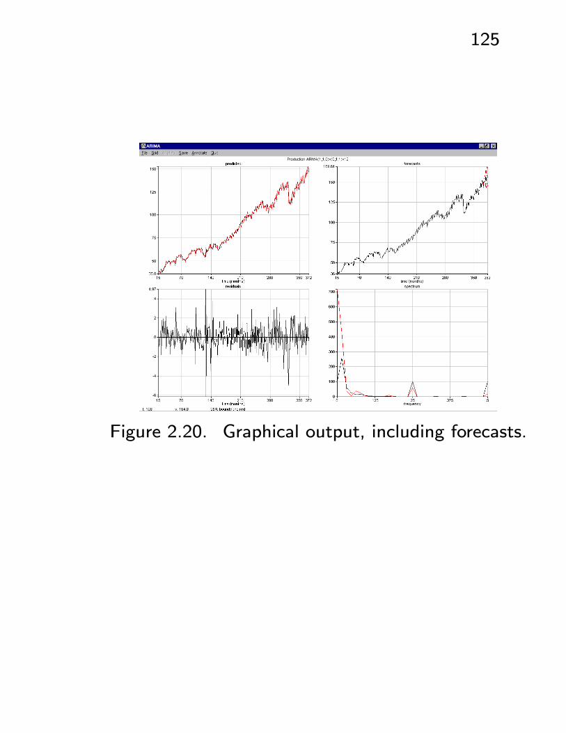
• See Figures 2.18 - 2.20.

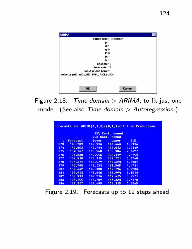
124

Figure 2.18. Time domain > ARIMA, to fit just one

model. (See also Time domain > Autoregression.)

Figure 2.19. Forecasts up to 12 steps ahead.

125

Figure 2.20. Graphical output, including forecasts.

126

14. Lecture 14 (Review)

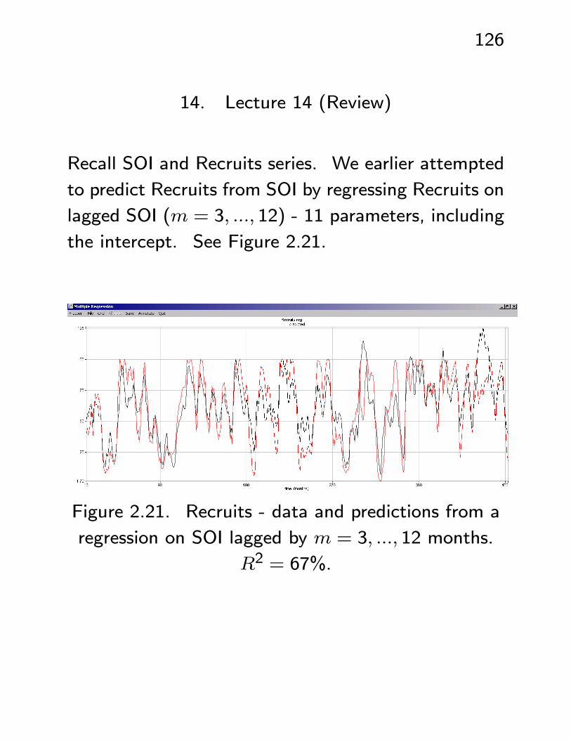
Recall SOI and Recruits series. We earlier attempted

to predict Recruits from SOI by regressing Recruits on

lagged SOI (m = 3, ..., 12) - 11 parameters, including

the intercept. See Figure 2.21.

Figure 2.21. Recruits - data and predictions from a

regression on SOI lagged by m = 3, ..., 12 months.

R2 = 67%.

127

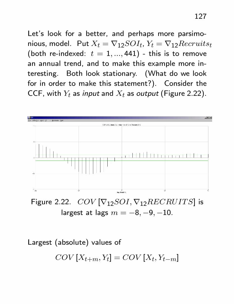
Let’s look for a better, and perhaps more parsimo-

nious, model. PutXt = ∇12SOIt, Yt = ∇12Recruitst(both re-indexed: t = 1, ..., 441) - this is to remove

an annual trend, and to make this example more in-

teresting. Both look stationary. (What do we look

for in order to make this statement?). Consider the

CCF, with Yt as input and Xt as output (Figure 2.22).

Figure 2.22. COV [∇12SOI,∇12RECRUITS] islargest at lags m = −8,−9,−10.

Largest (absolute) values of

COV [Xt+m, Yt] = COV [Xt, Yt−m]

128

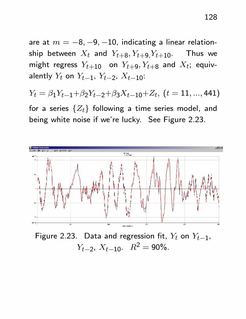
are at m = −8,−9,−10, indicating a linear relation-ship between Xt and Yt+8, Yt+9,Yt+10. Thus we

might regress Yt+10 on Yt+9, Yt+8 and Xt; equiv-

alently Yt on Yt−1, Yt−2, Xt−10:

Yt = β1Yt−1+β2Yt−2+β3Xt−10+Zt, (t = 11, ..., 441)

for a series {Zt} following a time series model, andbeing white noise if we’re lucky. See Figure 2.23.

Figure 2.23. Data and regression fit, Yt on Yt−1,Yt−2, Xt−10. R2 = 90%.

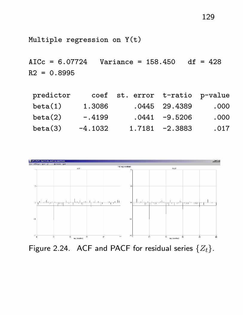
129

Multiple regression on Y(t)

AICc = 6.07724 Variance = 158.450 df = 428

R2 = 0.8995

predictor coef st. error t-ratio p-value

beta(1) 1.3086 .0445 29.4389 .000

beta(2) -.4199 .0441 -9.5206 .000

beta(3) -4.1032 1.7181 -2.3883 .017

Figure 2.24. ACF and PACF for residual series {Zt}.

130

The residual series {Zt} still exhibits some trends- see Figure 2.24 - seasonal ARMA(4, 1)12? ARIMA

Search, with AICc, selects ARMA(1, 1)12. With

BIC, ARMA(1, 2)12 is selected. Each of these was

fitted. Both failed the cumulative spectrum test, and

the Box-Pierce test with M −K = 1, although the p-

values at M −K = 20 were non-significant. (What

are these, and what do they test for? What does

“p-value” mean?) This suggested adding an AR(1)

term to the simpler of the two previous models.

In terms of the backshift operator (what is it? how

are these polynomials manipulated?):

(1− φB)³1−ΦB12

´Zt =

³1−ΘB12

´wt.

131

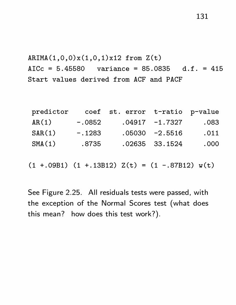
ARIMA(1,0,0)x(1,0,1)x12 from Z(t)

AICc = 5.45580 variance = 85.0835 d.f. = 415

Start values derived from ACF and PACF

predictor coef st. error t-ratio p-value

AR(1) -.0852 .04917 -1.7327 .083

SAR(1) -.1283 .05030 -2.5516 .011

SMA(1) .8735 .02635 33.1524 .000

(1 +.09B1) (1 +.13B12) Z(t) = (1 -.87B12) w(t)

See Figure 2.25. All residuals tests were passed, with

the exception of the Normal Scores test (what does

this mean? how does this test work?).

132

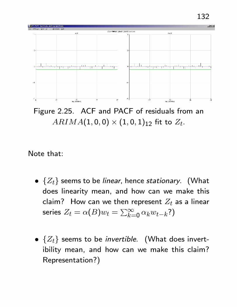
Figure 2.25. ACF and PACF of residuals from an

ARIMA(1, 0, 0)× (1, 0, 1)12 fit to Zt.

Note that:

• {Zt} seems to be linear, hence stationary. (Whatdoes linearity mean, and how can we make this

claim? How can we then represent Zt as a linear

series Zt = α(B)wt =P∞k=0αkwt−k?)

• {Zt} seems to be invertible. (What does invert-ibility mean, and how can we make this claim?

Representation?)

133

The polynomial β(B) = 1 − β1B − β2B2 has zeros

B = 1.34, 1.77. This yields the additional represen-

tation

Yt =β3B

10

β(B)Xt +

α(B)

β(B)wt

= β3γ(B)B10Xt + δ(B)wt,

with 1/β(B) expanded as a series γ(B) and δ(B) =

α(B)/β(B). Assume {wt} independent of {Xt, Yt}.

134

Predictions: You should be sufficiently familiar with

the prediction theory covered in class that you can

follow the following development, although I wouldn’t

expect you to come up with something like this on your

own. (The point of knowing the theory is so that you

can still do something sensible when the theory you

know doesn’t quite apply!)

The best forecast of Yt+l is Ytt+l = E

hYt+l|Y t

i(es-

timated), in the case of a single series {Yt}. (Why?

- you should be able to apply the Double Expectation

Theorem, so as to derive this result. And what does

“best” mean, in this context?)

135

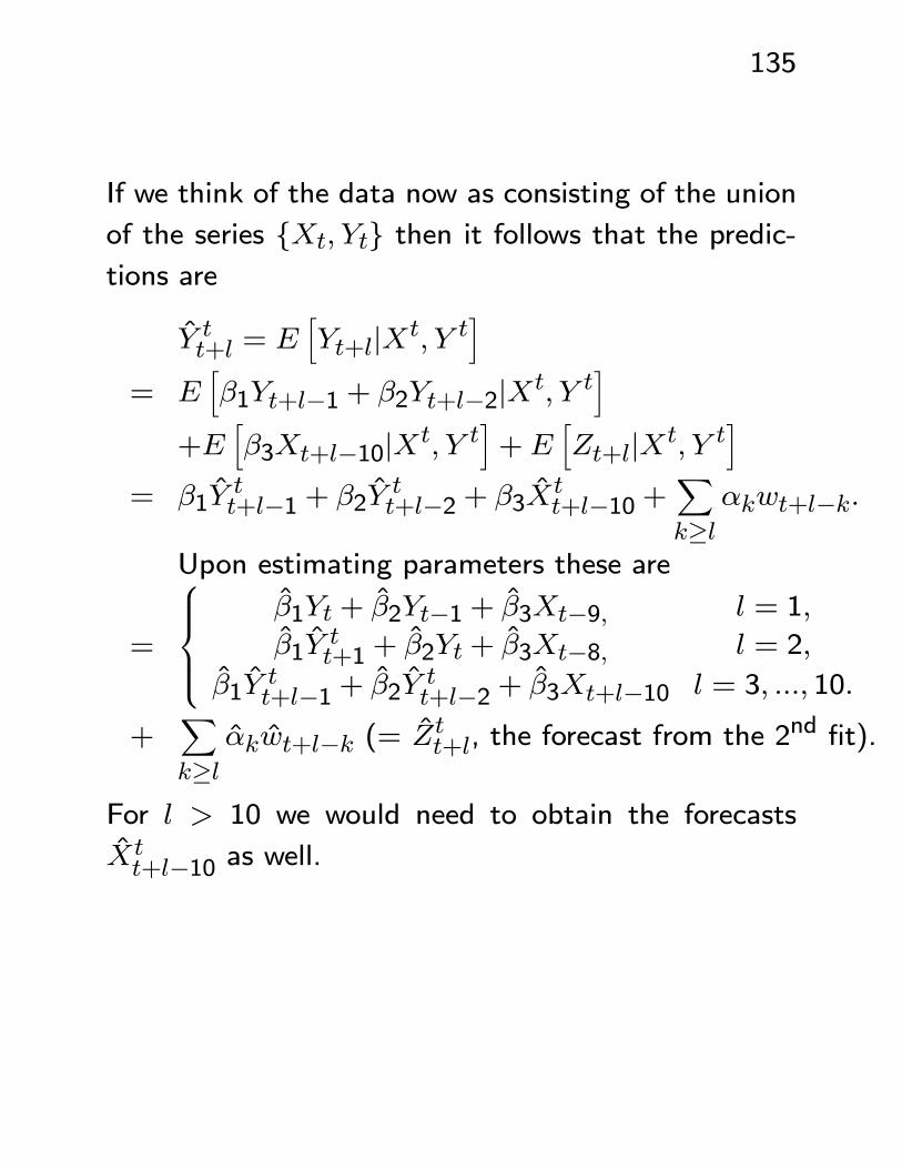
If we think of the data now as consisting of the union

of the series {Xt, Yt} then it follows that the predic-tions are

Y tt+l = E

hYt+l|Xt, Y t

i= E

hβ1Yt+l−1 + β2Yt+l−2|Xt, Y t

i+E

hβ3Xt+l−10|Xt, Y t

i+E

hZt+l|Xt, Y t

i= β1Y

tt+l−1 + β2Y

tt+l−2 + β3X

tt+l−10 +

Xk≥l

αkwt+l−k.

Upon estimating parameters these are

=

⎧⎪⎪⎨⎪⎪⎩β1Yt + β2Yt−1 + β3Xt−9, l = 1,

β1Ytt+1 + β2Yt + β3Xt−8, l = 2,

β1Ytt+l−1 + β2Y

tt+l−2 + β3Xt+l−10 l = 3, ..., 10.

+Xk≥l

αkwt+l−k (= Ztt+l, the forecast from the 2nd fit).

For l > 10 we would need to obtain the forecasts

Xtt+l−10 as well.

136

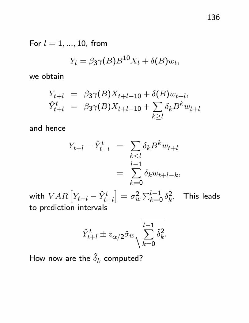
For l = 1, ..., 10, from

Yt = β3γ(B)B10Xt + δ(B)wt,

we obtain

Yt+l = β3γ(B)Xt+l−10 + δ(B)wt+l,

Y tt+l = β3γ(B)Xt+l−10 +

Xk≥l

δkBkwt+l

and hence

Yt+l − Y tt+l =

Xk<l

δkBkwt+l

=l−1Xk=0

δkwt+l−k,

with V ARhYt+l − Y t

t+l

i= σ2w

Pl−1k=0 δ

2k. This leads

to prediction intervals

Y tt+l ± zα/2σw

vuuut l−1Xk=0

δ2k.

How now are the δk computed?

137

Other theoretical things you should be familiar with:

• Calculations of ACFs (pretty simple for an MA;derive and solve the Yule-Walker equations for an

AR). What is the important property of the ACF

of an MA?

• Calculation of PACFs - define the PACF, then dothe required minimization. What is the impor-

tant property of the PACF of an AR?

• Maximum likelihood estimation

— The end result of our theoretical discussion

was that the MLEs of the AR and MA para-

meters φ and θ are the minimizers of the sum

of squares of the residuals:

S (φ,θ) =X

w2t (φ,θ) .

For a pure AR this is accomplished by a lin-

ear regression of the series on its own past.

138

If there are MA terms then an iterative pro-

cedure (Gauss-Newton) is necessary. As an

example, you should be able to show that, un-

der the usual assumption (what is it?), for an

MA(1) model you get

wt (θ) =t−1Xs=0

θsXt−s,

so that S (θ) is a polynomial in θ, of degree

2 (t− 1), to be minimized.What would you use as the starting estimate,

in the iterative procedure? How would the

iterations then be carried out? Your calcula-

tions should yield the iterative procedure

θk+1 = θk −Pwt (θk) wt (θk)P

w2t (θk).

139

— The usual estimate of the noise variance, ob-

tain by modifying the MLE, is

σ2w =S³φ, θ

´# of residuals − # of parameters

=

P(residuals)2

# of residuals − # of parameters.

— What is the “Information Matrix”, and what

role does it play in making inferences about

the parameters in an ARMA model?