Embed Size (px)
Citation preview
Portfolio inference and portfolio overfit
Steven E. [email protected]
Formerly of Cerebellum Capital
Sep 10, 2015
Steven Pav (gilgamath) Portfolio Inference ... Sep 10, 2015 1 / 52
Portfolios
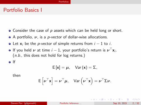
Portfolio Basics I
Consider the case of p assets which can be held long or short.
A portfolio, ν, is a p-vector of dollar-wise allocations.
Let xi be the p-vector of simple returns from i − 1 to i .
If you held ν at time i − 1, your portfolio’s return is ν>xi .(n.b., this does not hold for log returns.)
If
E [x] = µ, Var (x) = Σ,
then
E[ν>x
]= ν>µ, Var
(ν>x
)= ν>Σν.
Steven Pav (gilgamath) Portfolio Inference ... Sep 10, 2015 2 / 52
Portfolios
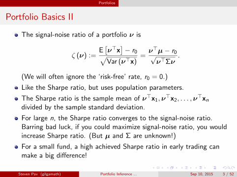
Portfolio Basics II
The signal-noise ratio of a portfolio ν is
ζ (ν) :=E[ν>x
]− r0√
Var (ν>x)=
ν>µ− r0√ν>Σν
.
(We will often ignore the ‘risk-free’ rate, r0 = 0.)
Like the Sharpe ratio, but uses population parameters.
The Sharpe ratio is the sample mean of ν>x1,ν>x2, . . . ,ν
>xn
divided by the sample standard deviation.
For large n, the Sharpe ratio converges to the signal-noise ratio.Barring bad luck, if you could maximize signal-noise ratio, you wouldincrease Sharpe ratio. (But µ and Σ are unknown!)
For a small fund, a high achieved Sharpe ratio in early trading canmake a big difference!
Steven Pav (gilgamath) Portfolio Inference ... Sep 10, 2015 3 / 52
Portfolios
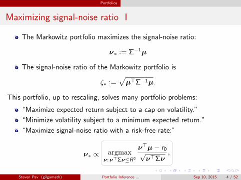
Maximizing signal-noise ratio I
The Markowitz portfolio maximizes the signal-noise ratio:
ν∗ := Σ−1µ
The signal-noise ratio of the Markowitz portfolio is
ζ∗ :=√µ>Σ−1µ.
This portfolio, up to rescaling, solves many portfolio problems:
“Maximize expected return subject to a cap on volatility.”
“Minimize volatility subject to a minimum expected return.”
“Maximize signal-noise ratio with a risk-free rate:”
ν∗ ∝ argmaxν:ν>Σν≤R2
ν>µ− r0√ν>Σν
,
Steven Pav (gilgamath) Portfolio Inference ... Sep 10, 2015 4 / 52

Portfolio Inference
A weird trick
Prepend a ‘1’ to the vector: x :=[1, x>
]>.
The second moment of x contains the first two moments of x:
Θ := E[xx>
]=
[1 µ>
µ Σ + µµ>
].
then: Θ−1 =
[1 + µ>Σ−1µ −µ>Σ−1
−Σ−1µ Σ−1
]
=
1 + ζ2∗ −ν∗>
−ν∗ Σ−1
,ν∗ is the Markowitz portfolio,
ζ∗ is the signal-noise ratio of ν∗.
Σ−1 is the ‘precision matrix’.
Steven Pav (gilgamath) Portfolio Inference ... Sep 10, 2015 5 / 52
Portfolio Inference
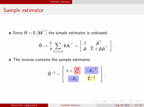
Sample estimator
Since Θ = E[xx>
]the simple estimator is unbiased:
Θ :=1
n
∑1≤i≤n
xi xi> =
[1 µ>
µ Σ + µµ>
].
The inverse contains the sample estimates:
Θ−1 =
1 + ζ2∗ −ν∗>
−ν∗ Σ−1
.
Steven Pav (gilgamath) Portfolio Inference ... Sep 10, 2015 6 / 52
Portfolio Inference
Asymptotics I
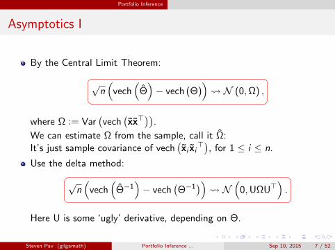
By the Central Limit Theorem:
√n(
vech(
Θ)− vech (Θ)
) N (0,Ω) ,
where Ω := Var(vech
(xx>
)).
We can estimate Ω from the sample, call it Ω:It’s just sample covariance of vech
(xi xi
>), for 1 ≤ i ≤ n.
Use the delta method:
√n(
vech(
Θ−1)− vech
(Θ−1
)) N
(0,UΩU>
).
Here U is some ‘ugly’ derivative, depending on Θ.
Steven Pav (gilgamath) Portfolio Inference ... Sep 10, 2015 7 / 52
Portfolio Inference
Asymptotics II
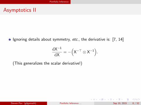
Ignoring details about symmetry, etc., the derivative is: [7, 14]
dX−1
dX= −
(X−> ⊗ X−1
).
(This generalizes the scalar derivative!)
Steven Pav (gilgamath) Portfolio Inference ... Sep 10, 2015 8 / 52
Portfolio Inference
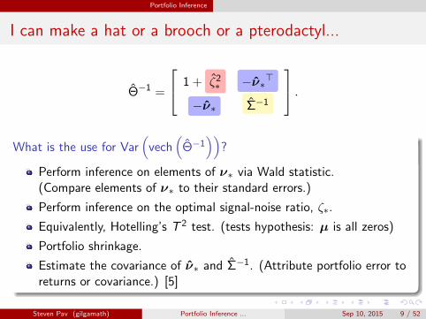
I can make a hat or a brooch or a pterodactyl...
Θ−1 =
1 + ζ2∗ −ν∗>
−ν∗ Σ−1
.What is the use for Var
(vech
(Θ−1
))?
Perform inference on elements of ν∗ via Wald statistic.(Compare elements of ν∗ to their standard errors.)
Perform inference on the optimal signal-noise ratio, ζ∗.
Equivalently, Hotelling’s T 2 test. (tests hypothesis: µ is all zeros)
Portfolio shrinkage.
Estimate the covariance of ν∗ and Σ−1. (Attribute portfolio error toreturns or covariance.) [5]
Steven Pav (gilgamath) Portfolio Inference ... Sep 10, 2015 9 / 52
Portfolio Inference
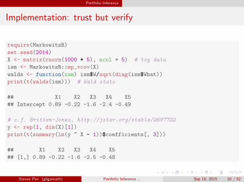
Implementation: trust but verify
require(MarkowitzR)
set.seed(2014)
X <- matrix(rnorm(1000 * 5), ncol = 5) # toy data
ism <- MarkowitzR::mp_vcov(X)
walds <- function(ism) ism$W/sqrt(diag(ism$What))
print(t(walds(ism))) # Wald stats
## X1 X2 X3 X4 X5
## Intercept 0.89 -0.22 -1.6 -2.4 -0.49
# c.f. Britten-Jones, http://jstor.org/stable/2697722
y <- rep(1, dim(X)[1])
print(t(summary(lm(y ~ X - 1))$coefficients[, 3]))
## X1 X2 X3 X4 X5
## [1,] 0.89 -0.22 -1.6 -2.5 -0.48
Steven Pav (gilgamath) Portfolio Inference ... Sep 10, 2015 10 / 52
Portfolio Inference
Selling this weird trick
Why weird trick, not Britten-Jones, or Okhrin et al.? [4, 2, 15]
Fewer assumptions: fourth moments exist vs. normality of returns.
Straightforward to use HAC estimator for Ω.
Models covariance between return and volatility. (At a cost?)
Solves a larger problem, e.g., can use for inference on ζ2∗ .
Real question: what’s wrong with vanilla Markowitz?
This trick can be adapted to deal with:
Hedged portfolios.
Heteroskedasticity.
Conditional expected returns.
Perhaps more ...
Steven Pav (gilgamath) Portfolio Inference ... Sep 10, 2015 11 / 52
Extensions
Hedged portfolios I
Hedging: the goal
Returns which are statistically independent from some random variables.
Hedging: a more realistic goal
A portfolio with zero covariance to some random variables.
Hedging: an achievable goal
A portfolio with zero sample covariance to some other portfolios oftradeable assets.(e.g., you may have to hold some Mkt to hedge out the Mkt.)
Steven Pav (gilgamath) Portfolio Inference ... Sep 10, 2015 12 / 52
Extensions
Hedged portfolios II
maxν:GΣν=0,ν>Σν≤R2
ν>µ− r0√ν>Σν
,
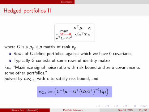
where G is a pg × p matrix of rank pg .
Rows of G define portfolios against which we have 0 covariance.
Typically G consists of some rows of identity matrix.
i.e., “Maximize signal-noise ratio with risk bound and zero covariance tosome other portfolios.”Solved by cνG,∗, with c to satisfy risk bound, and
νG,∗ :=(
Σ−1µ− G>(GΣG>
)−1Gµ).
Steven Pav (gilgamath) Portfolio Inference ... Sep 10, 2015 13 / 52
Extensions
Hedged portfolios III
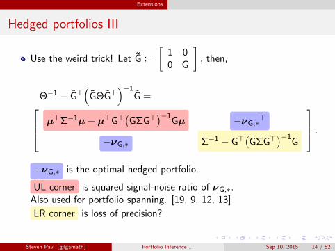
Use the weird trick! Let G :=
[1 00 G
], then,
Θ−1 − G>(
GΘG>)−1
G = µ>Σ−1µ− µ>G>(GΣG>
)−1Gµ −νG,∗
>
−νG,∗ Σ−1 − G>(GΣG>
)−1G
.−νG,∗ is the optimal hedged portfolio.
UL corner is squared signal-noise ratio of νG,∗.Also used for portfolio spanning. [19, 9, 12, 13]
LR corner is loss of precision?
Steven Pav (gilgamath) Portfolio Inference ... Sep 10, 2015 14 / 52
Extensions
Hedged portfolios IV
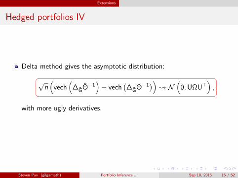
Delta method gives the asymptotic distribution:
√n(
vech(
∆GΘ−1)− vech
(∆GΘ−1
)) N
(0,UΩU>
),
with more ugly derivatives.
Steven Pav (gilgamath) Portfolio Inference ... Sep 10, 2015 15 / 52
Extensions
Hedged portfolios V
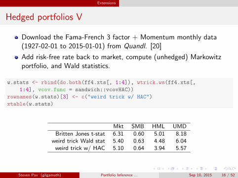
Download the Fama-French 3 factor + Momentum monthly data(1927-02-01 to 2015-01-01) from Quandl. [20]
Add risk-free rate back to market, compute (unhedged) Markowitzportfolio, and Wald statistics.
w.stats <- rbind(do.both(ff4.xts[, 1:4]), wtrick.ws(ff4.xts[,
1:4], vcov.func = sandwich::vcovHAC))
rownames(w.stats)[3] <- c("weird trick w/ HAC")
xtable(w.stats)
Mkt SMB HML UMD
Britten Jones t-stat 6.31 0.60 5.01 8.18weird trick Wald stat 5.40 0.63 4.48 6.04weird trick w/ HAC 5.10 0.64 3.94 5.57
Steven Pav (gilgamath) Portfolio Inference ... Sep 10, 2015 16 / 52
Extensions
Hedged portfolios VI
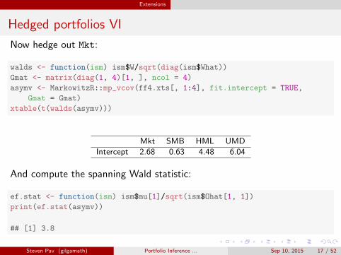
Now hedge out Mkt:
walds <- function(ism) ism$W/sqrt(diag(ism$What))
Gmat <- matrix(diag(1, 4)[1, ], ncol = 4)
asymv <- MarkowitzR::mp_vcov(ff4.xts[, 1:4], fit.intercept = TRUE,
Gmat = Gmat)
xtable(t(walds(asymv)))
Mkt SMB HML UMD
Intercept 2.68 0.63 4.48 6.04
And compute the spanning Wald statistic:
ef.stat <- function(ism) ism$mu[1]/sqrt(ism$Ohat[1, 1])
print(ef.stat(asymv))
## [1] 3.8
Steven Pav (gilgamath) Portfolio Inference ... Sep 10, 2015 17 / 52
Extensions
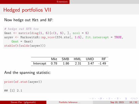
Hedged portfolios VII
Now hedge out Mkt and RF:
# hedge out RFR too
Gmat <- matrix(diag(1, 5)[c(1, 5), ], ncol = 5)
asymv <- MarkowitzR::mp_vcov(ff4.xts[, 1:5], fit.intercept = TRUE,
Gmat = Gmat)
xtable(t(walds(asymv)))
Mkt SMB HML UMD RF
Intercept 0.78 1.86 2.31 3.47 -1.49
And the spanning statistic:
print(ef.stat(asymv))
## [1] 2.1
Steven Pav (gilgamath) Portfolio Inference ... Sep 10, 2015 18 / 52
Extensions
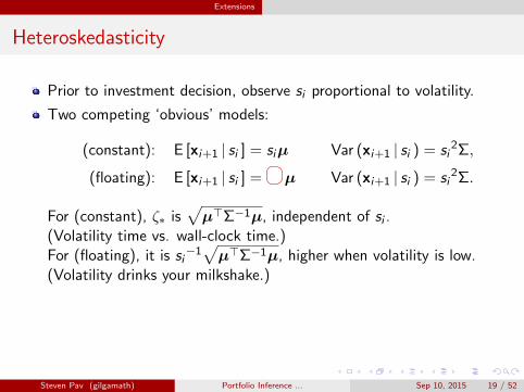
Heteroskedasticity
Prior to investment decision, observe si proportional to volatility.
Two competing ‘obvious’ models:
(constant): E [xi+1 | si ] = siµ Var (xi+1 | si ) = si2Σ,
(floating): E [xi+1 | si ] = µ Var (xi+1 | si ) = si2Σ.
For (constant), ζ∗ is√µ>Σ−1µ, independent of si .
(Volatility time vs. wall-clock time.)For (floating), it is si
−1√µ>Σ−1µ, higher when volatility is low.
(Volatility drinks your milkshake.)
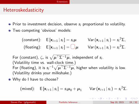
Why do I have to choose?
(mixed): E [xi+1 | si ] = siµ0 + µ1 Var (xi+1 | si ) = si2Σ.
Steven Pav (gilgamath) Portfolio Inference ... Sep 10, 2015 19 / 52
Extensions
Heteroskedasticity
Prior to investment decision, observe si proportional to volatility.
Two competing ‘obvious’ models:
(constant): E [xi+1 | si ] = siµ Var (xi+1 | si ) = si2Σ,
(floating): E [xi+1 | si ] = µ Var (xi+1 | si ) = si2Σ.
For (constant), ζ∗ is√µ>Σ−1µ, independent of si .
(Volatility time vs. wall-clock time.)For (floating), it is si
−1√µ>Σ−1µ, higher when volatility is low.
(Volatility drinks your milkshake.)
Why do I have to choose?
(mixed): E [xi+1 | si ] = siµ0 + µ1 Var (xi+1 | si ) = si2Σ.
Steven Pav (gilgamath) Portfolio Inference ... Sep 10, 2015 19 / 52
Extensions
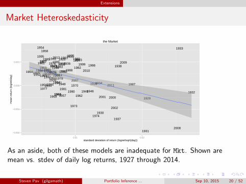
Market Heteroskedasticity
19271928
1929
1930
1931
1932
1933
1934
1935
1936
1937
1938
1939
19401941
1942
19431944
1945
1946
19471948
1949
1950
1951
1952
1953
1954
1955
1956
1957
1958
1959
1960
1961
1962
196319641965
1966
1967
1968
1969
1970
19711972
1973
1974
1975
1976
1977
1978
1979
1980
1981
19821983
1984
1985
1986
1987
1988
1989
1990
1991
19921993
1994
1995
1996
1997
19981999
20002001
2002
2003
2004
2005
2006
2007
2008
2009
2010
2011
2012
2013
2014
−0.002
−0.001
0.000
0.001
0.01 0.02standard deviation of return (logret/sqrt(day))
mea
n re
turn
(lo
gret
/day
)
the Market
As an aside, both of these models are inadequate for Mkt. Shown aremean vs. stdev of daily log returns, 1927 through 2014.
Steven Pav (gilgamath) Portfolio Inference ... Sep 10, 2015 20 / 52
Extensions
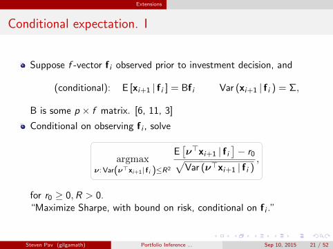
Conditional expectation. I
Suppose f -vector f i observed prior to investment decision, and
(conditional): E [xi+1 | f i ] = Bf i Var (xi+1 | f i ) = Σ,
B is some p × f matrix. [6, 11, 3]
Conditional on observing f i , solve
argmaxν: Var(ν>xi+1| f i )≤R2
E[ν>xi+1 | f i
]− r0√
Var (ν>xi+1 | f i ),
for r0 ≥ 0,R > 0.“Maximize Sharpe, with bound on risk, conditional on f i .”
Steven Pav (gilgamath) Portfolio Inference ... Sep 10, 2015 21 / 52
Extensions
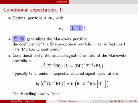
Conditional expectation. II
Optimal portfolio is cν∗ with
ν∗ := Σ−1B f i .
Σ−1B generalizes the Markowitz portfolio:the coefficient of the Sharpe-optimal portfolio linear in features f i .The ‘Markowitz coefficient.’
Conditional on f i , the squared signal-noise ratio of the Markowitzportfolio is
ζ2(Σ−1Bf i
)| f i = (Bf i )
>Σ−1 (Bf i ) .
Typically f i is random. Expected squared signal-noise ratio is
Ef
[ζ2(Σ−1Bf i
)]= tr
(B>Σ−1B E
[ff>]).
The Hotelling-Lawley Trace.
Steven Pav (gilgamath) Portfolio Inference ... Sep 10, 2015 22 / 52
Extensions
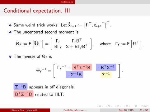
Conditional expectation. III
Same weird trick works! Let ˜xi+1 :=[f i>, xi+1
>]>.The uncentered second moment is
Θf := E[˜x˜x>]
=
[Γf Γf B>
BΓf Σ + BΓf B>
], where Γf := E
[ff>].
The inverse of Θf is
Θf−1 =
[Γf−1 + B>Σ−1B −B>Σ−1
−Σ−1B Σ−1
].
Σ−1B appears in off diagonals.
B>Σ−1B related to HLT.
Steven Pav (gilgamath) Portfolio Inference ... Sep 10, 2015 23 / 52
Extensions
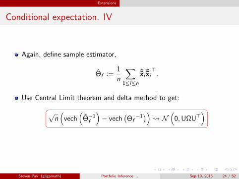
Conditional expectation. IV
Again, define sample estimator,
Θf :=1
n
∑1≤i≤n
˜xi˜xi>.
Use Central Limit theorem and delta method to get:
√n(
vech(
Θ−1f
)− vech
(Θf−1)) N
(0,UΩU>
)
Steven Pav (gilgamath) Portfolio Inference ... Sep 10, 2015 24 / 52
Examples
Examples. I
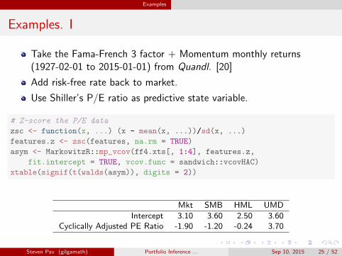
Take the Fama-French 3 factor + Momentum monthly returns(1927-02-01 to 2015-01-01) from Quandl. [20]
Add risk-free rate back to market.
Use Shiller’s P/E ratio as predictive state variable.
# Z-score the P/E data
zsc <- function(x, ...) (x - mean(x, ...))/sd(x, ...)
features.z <- zsc(features, na.rm = TRUE)
asym <- MarkowitzR::mp_vcov(ff4.xts[, 1:4], features.z,
fit.intercept = TRUE, vcov.func = sandwich::vcovHAC)
xtable(signif(t(walds(asym)), digits = 2))
Mkt SMB HML UMD
Intercept 3.10 3.60 2.50 3.60Cyclically Adjusted PE Ratio -1.90 -1.20 -0.24 3.70
Steven Pav (gilgamath) Portfolio Inference ... Sep 10, 2015 25 / 52
Examples
Examples. II
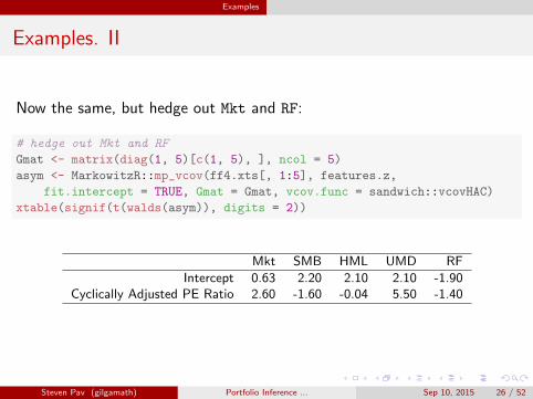
Now the same, but hedge out Mkt and RF:
# hedge out Mkt and RF
Gmat <- matrix(diag(1, 5)[c(1, 5), ], ncol = 5)
asym <- MarkowitzR::mp_vcov(ff4.xts[, 1:5], features.z,
fit.intercept = TRUE, Gmat = Gmat, vcov.func = sandwich::vcovHAC)
xtable(signif(t(walds(asym)), digits = 2))
Mkt SMB HML UMD RF
Intercept 0.63 2.20 2.10 2.10 -1.90Cyclically Adjusted PE Ratio 2.60 -1.60 -0.04 5.50 -1.40
Steven Pav (gilgamath) Portfolio Inference ... Sep 10, 2015 26 / 52
Examples
Examples. III
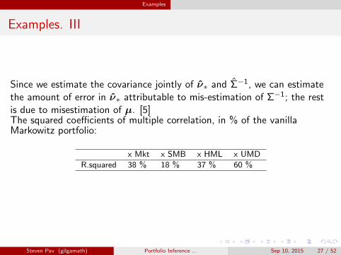
Since we estimate the covariance jointly of ν∗ and Σ−1, we can estimatethe amount of error in ν∗ attributable to mis-estimation of Σ−1; the restis due to misestimation of µ. [5]The squared coefficients of multiple correlation, in % of the vanillaMarkowitz portfolio:
x Mkt x SMB x HML x UMD
R.squared 38 % 18 % 37 % 60 %
Steven Pav (gilgamath) Portfolio Inference ... Sep 10, 2015 27 / 52
Segue
What else?
The same basic model can be adapted to:
Constrained estimation of Θ. (Linear constraints; rank constraints?)
Conditional covariance and conditional beta. [8]
Steven Pav (gilgamath) Portfolio Inference ... Sep 10, 2015 28 / 52

Segue
Segue
Steven Pav (gilgamath) Portfolio Inference ... Sep 10, 2015 29 / 52
Segue
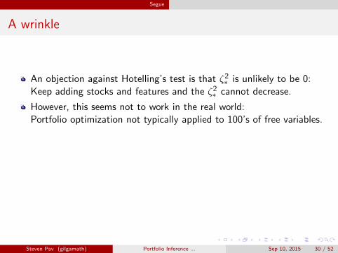
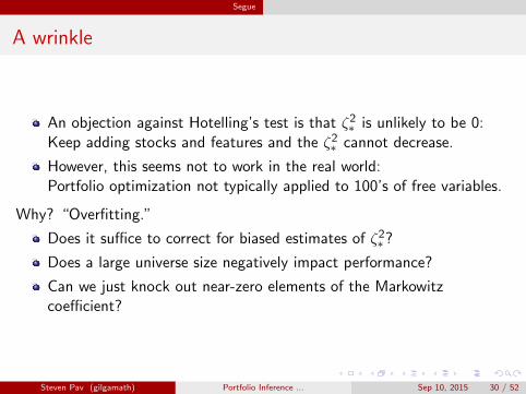
A wrinkle
An objection against Hotelling’s test is that ζ2∗ is unlikely to be 0:
Keep adding stocks and features and the ζ2∗ cannot decrease.
However, this seems not to work in the real world:Portfolio optimization not typically applied to 100’s of free variables.
Why? “Overfitting.”
Does it suffice to correct for biased estimates of ζ2∗?
Does a large universe size negatively impact performance?
Can we just knock out near-zero elements of the Markowitzcoefficient?
Steven Pav (gilgamath) Portfolio Inference ... Sep 10, 2015 30 / 52
Segue
A wrinkle
An objection against Hotelling’s test is that ζ2∗ is unlikely to be 0:
Keep adding stocks and features and the ζ2∗ cannot decrease.
However, this seems not to work in the real world:Portfolio optimization not typically applied to 100’s of free variables.
Why? “Overfitting.”
Does it suffice to correct for biased estimates of ζ2∗?
Does a large universe size negatively impact performance?
Can we just knock out near-zero elements of the Markowitzcoefficient?
Steven Pav (gilgamath) Portfolio Inference ... Sep 10, 2015 30 / 52
Portfolio Overfit
Portfolio on a sphere?
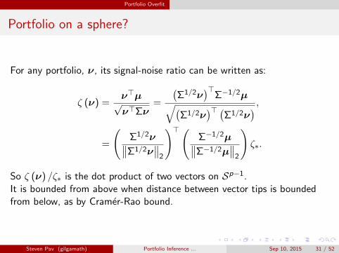
For any portfolio, ν, its signal-noise ratio can be written as:
ζ (ν) =ν>µ√ν>Σν
=
(Σ1/2ν
)>Σ−1/2µ√(
Σ1/2ν)> (
Σ1/2ν) ,
=
(Σ1/2ν∥∥Σ1/2ν
∥∥2
)>(Σ−1/2µ∥∥Σ−1/2µ
∥∥2
)ζ∗.
So ζ (ν) /ζ∗ is the dot product of two vectors on Sp−1.It is bounded from above when distance between vector tips is boundedfrom below, as by Cramer-Rao bound.
Steven Pav (gilgamath) Portfolio Inference ... Sep 10, 2015 31 / 52

Portfolio Overfit
Portfolio on a sphere?
sample: Σ1/2ν
optimal: Σ−1/2µ
Steven Pav (gilgamath) Portfolio Inference ... Sep 10, 2015 32 / 52
Portfolio Overfit
A Theorem I
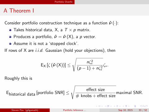
Consider portfolio construction technique as a function ν (·):
Takes historical data, X, a T × p matrix.
Produces a portfolio, ν = ν (X), a p vector.
Assume it is not a ‘stopped clock’.
If rows of X are i.i.d. Gaussian (hold your objections), then
EX [ζ (ν (X))] ≤
√nζ2∗
(p − 1) + nζ2∗ζ∗.
Roughly this is
Ehistorical data [portfolio SNR] ≤
√effect size
# knobs + effect sizemaximal SNR.
Steven Pav (gilgamath) Portfolio Inference ... Sep 10, 2015 33 / 52
Portfolio Overfit
A Theorem II
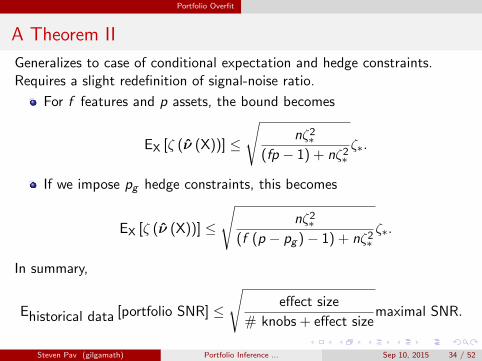
Generalizes to case of conditional expectation and hedge constraints.Requires a slight redefinition of signal-noise ratio.
For f features and p assets, the bound becomes
EX [ζ (ν (X))] ≤
√nζ2∗
(fp − 1) + nζ2∗ζ∗.
If we impose pg hedge constraints, this becomes
EX [ζ (ν (X))] ≤
√nζ2∗
(f (p − pg )− 1) + nζ2∗ζ∗.
In summary,
Ehistorical data [portfolio SNR] ≤
√effect size
# knobs + effect sizemaximal SNR.
Steven Pav (gilgamath) Portfolio Inference ... Sep 10, 2015 34 / 52
Portfolio Overfit
No Stopped Clocks
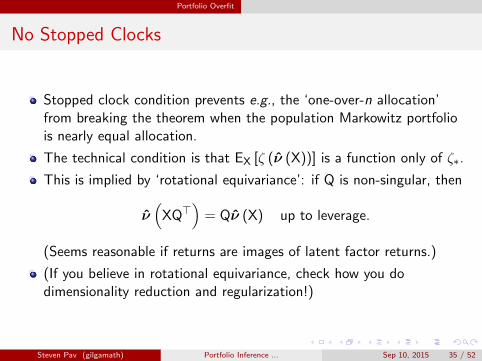
Stopped clock condition prevents e.g., the ‘one-over-n allocation’from breaking the theorem when the population Markowitz portfoliois nearly equal allocation.
The technical condition is that EX [ζ (ν (X))] is a function only of ζ∗.
This is implied by ‘rotational equivariance’: if Q is non-singular, then
ν(
XQ>)
= Qν (X) up to leverage.
(Seems reasonable if returns are images of latent factor returns.)
(If you believe in rotational equivariance, check how you dodimensionality reduction and regularization!)
Steven Pav (gilgamath) Portfolio Inference ... Sep 10, 2015 35 / 52
Portfolio Overfit
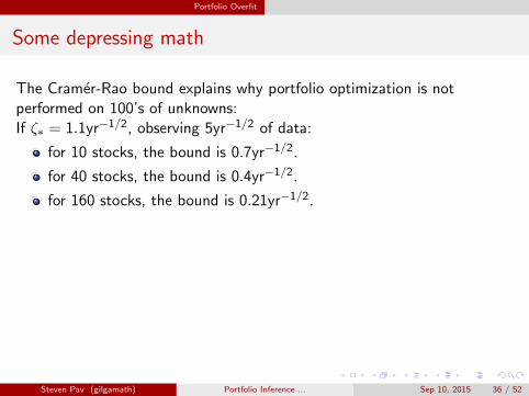
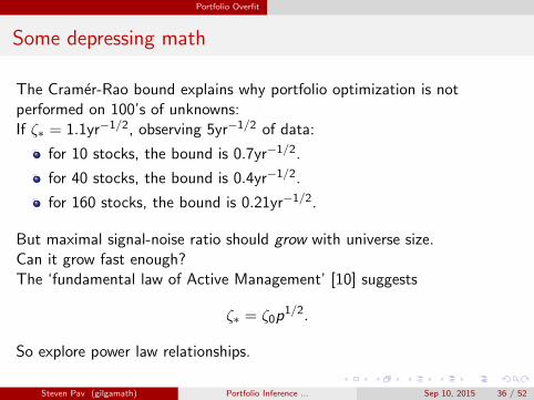
Some depressing math
The Cramer-Rao bound explains why portfolio optimization is notperformed on 100’s of unknowns:If ζ∗ = 1.1yr−1/2, observing 5yr−1/2 of data:
for 10 stocks, the bound is 0.7yr−1/2.
for 40 stocks, the bound is 0.4yr−1/2.
for 160 stocks, the bound is 0.21yr−1/2.
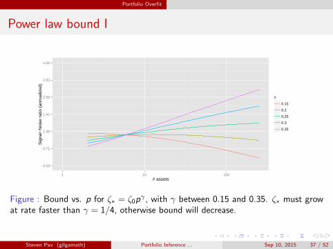
But maximal signal-noise ratio should grow with universe size.Can it grow fast enough?The ‘fundamental law of Active Management’ [10] suggests
ζ∗ = ζ0p1/2.
So explore power law relationships.
Steven Pav (gilgamath) Portfolio Inference ... Sep 10, 2015 36 / 52
Portfolio Overfit
Some depressing math
The Cramer-Rao bound explains why portfolio optimization is notperformed on 100’s of unknowns:If ζ∗ = 1.1yr−1/2, observing 5yr−1/2 of data:
for 10 stocks, the bound is 0.7yr−1/2.
for 40 stocks, the bound is 0.4yr−1/2.
for 160 stocks, the bound is 0.21yr−1/2.
But maximal signal-noise ratio should grow with universe size.Can it grow fast enough?The ‘fundamental law of Active Management’ [10] suggests
ζ∗ = ζ0p1/2.
So explore power law relationships.
Steven Pav (gilgamath) Portfolio Inference ... Sep 10, 2015 36 / 52
Portfolio Overfit
Power law bound I
0.50
0.71
1.00
1.41
2.00
2.83
4.00
1 10 100# assets
Sig
nal−
Noi
se r
atio
(an
nual
ized
)
γ
0.15
0.2
0.25
0.3
0.35
Figure : Bound vs. p for ζ∗ = ζ0pγ , with γ between 0.15 and 0.35. ζ∗ must grow
at rate faster than γ = 1/4, otherwise bound will decrease.
Steven Pav (gilgamath) Portfolio Inference ... Sep 10, 2015 37 / 52
Portfolio Overfit
Power law bound II
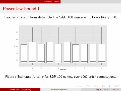
Idea: estimate γ from data. On the S&P 100 universe, it looks like γ = 0:
0.6
0.8
1.0
1.2
1.4
1 2 3 4 5 6 7 8 9 10# assets
ζ *
Figure : Estimated ζ∗ vs. p for S&P 100 names, over 1000 order permutations.
Steven Pav (gilgamath) Portfolio Inference ... Sep 10, 2015 38 / 52
Portfolio Overfit
Philosophical Q&A
“What does this say about my portfolio?”
Nothing. It is a frequentist argument about your method of constructingportfolios. It does not condition on e.g., ζ2
∗ . If ζ2∗ is ‘large’ compared to
degrees of freedom, the bound may not be an issue.
“Can I use historical data to reduce the degrees of freedom, and escapethe bound?”
Probably not. By using historical data, you subject yourself to the boundor your meta-method is a stopped clock.
“A rational agent cannot be harmed by more data, opportunities.”
This is a bad definition, or rational agents cannot exist, or they hold onlythe market portfolio.
Steven Pav (gilgamath) Portfolio Inference ... Sep 10, 2015 39 / 52
Portfolio Overfit
Future work
Compute confidence intervals on signal-noise ratio of a portfolio?
Is there a sensible Bayesian version of this result?
Can we sensibly perform dimensionality reduction using historical dataand avoid this ‘overfitting’?
Is there a more general result which really captures ‘effect size’ and‘number of knobs’?
Get a bound on variance of signal-noise ratio of portfolios?
Prove the bound is worse for returns with fatter tails?
Thank You.
Steven Pav (gilgamath) Portfolio Inference ... Sep 10, 2015 40 / 52

Appendix
Bibliography I
[1] Clifford S. Asness, Andrea Frazzini, Ronen Israel, and Tobias J. Moskowitz. Fact, fiction and momentum investing.Privately Published, May 2014. URL http://ssrn.com/abstract=2435323.
[2] Taras Bodnar and Yarema Okhrin. On the product of inverse Wishart and normal distributions with applications todiscriminant analysis and portfolio theory. Scandinavian Journal of Statistics, 38(2):311–331, 2011. ISSN 1467-9469. doi:10.1111/j.1467-9469.2011.00729.x. URL http://dx.doi.org/10.1111/j.1467-9469.2011.00729.x.
[3] Michael W Brandt. Portfolio choice problems. Handbook of financial econometrics, 1:269–336, 2009. URLhttps://faculty.fuqua.duke.edu/~mbrandt/papers/published/portreview.pdf.
[4] Mark Britten-Jones. The sampling error in estimates of mean-variance efficient portfolio weights. The Journal of Finance,54(2):655–671, 1999. URL http://www.jstor.org/stable/2697722.
[5] Vijay Kumar Chopra and William T. Ziemba. The effect of errors in means, variances, and covariances on optimal portfoliochoice. The Journal of Portfolio Management, 19(2):6–11, 1993. URLhttp://faculty.fuqua.duke.edu/~charvey/Teaching/BA453_2006/Chopra_The_effect_of_1993.pdf.
[6] Gregory Connor. Sensible return forecasting for portfolio management. Financial Analysts Journal, 53(5):pp. 44–51, 1997.ISSN 0015198X. URL https:
//faculty.fuqua.duke.edu/~charvey/Teaching/BA453_2006/Connor_Sensible_Return_Forecasting_1997.pdf.
[7] Paul L. Fackler. Notes on matrix calculus. Privately Published, 2005. URLhttp://www4.ncsu.edu/~pfackler/MatCalc.pdf.
[8] Wayne E. Ferson and Campbell R. Harvey. Conditioning variables and the cross-section of stock returns. Technical report,Fuqua School of Business Working Paper No. 9902, February 1999. URL http://ssrn.com/abstract=152910.
[9] Narayan C. Giri. On the likelihood ratio test of a normal multivariate testing problem. The Annals of MathematicalStatistics, 35(1):181–189, 1964. doi: 10.1214/aoms/1177703740. URLhttp://projecteuclid.org/euclid.aoms/1177703740.
[10] R. Grinold and R. Kahn. Active Portfolio Management: A Quantitative Approach for Producing Superior Returns andSelecting Superior Returns and Controlling Risk. McGraw-Hill Library of Investment and Finance. McGraw-Hill Education,1999. ISBN 9780070248823. URL http://books.google.com/books?id=a1yB8LTQnOEC.
Steven Pav (gilgamath) Portfolio Inference ... Sep 10, 2015 41 / 52

Appendix
Bibliography II
[11] Ulf Herold and Raimond Maurer. Tactical asset allocation and estimation risk. Financial Markets and PortfolioManagement, 18(1):39–57, 2004. ISSN 1555-4961. doi: 10.1007/s11408-004-0104-2. URLhttp://dx.doi.org/10.1007/s11408-004-0104-2.
[12] Gur Huberman and Shmuel Kandel. Mean-variance spanning. The Journal of Finance, 42(4):pp. 873–888, 1987. ISSN00221082. URL http://www.jstor.org/stable/2328296.
[13] Raymond Kan and GuoFu Zhou. Tests of mean-variance spanning. Annals of Economics and Finance, 13(1), 2012. URLhttp://www.aeconf.net/Articles/May2012/aef130105.pdf.
[14] Jan R. Magnus and H. Neudecker. Matrix Differential Calculus with Applications in Statistics and Econometrics. WileySeries in Probability and Statistics: Texts and References Section. Wiley, 3rd edition, 2007. ISBN 9780471986331. URLhttp://www.janmagnus.nl/misc/mdc2007-3rdedition.
[15] Yarema Okhrin and Wolfgang Schmid. Distributional properties of portfolio weights. Journal of Econometrics, 134(1):235–256, 2006. URL http://www.sciencedirect.com/science/article/pii/S0304407605001442.
[16] Steven E. Pav. Asymptotic distribution of the Markowitz portfolio. Privately Published, 2013. URLhttp://arxiv.org/abs/1312.0557.
[17] Steven E. Pav. Bounds on portfolio quality. Privately Published, 2014. URL http://arxiv.org/abs/1409.5936.
[18] Steven E. Pav. MarkowitzR: Statistical Significance of the Markowitz Portfolio, 2015. URLhttps://github.com/shabbychef/MarkowitzR. R package version 0.1502.
[19] C. Radhakrishna Rao. Advanced Statistical Methods in Biometric Research. John Wiley and Sons, 1952. URLhttp://books.google.com/books?id=HvFLAAAAMAAJ.
[20] Raymond McTaggart and Gergely Daroczi. Quandl: API Wrapper for Quandl.com, 2015. URLhttp://CRAN.R-project.org/package=Quandl. R package version 2.6.0.
[21] A. D. Roy. Safety first and the holding of assets. Econometrica, 20(3):pp. 431–449, 1952. ISSN 00129682. URLhttp://www.jstor.org/stable/1907413.
[22] Mervyn J. Silvapulle and Pranab Kumar Sen. Constrained statistical inference : inequality, order, and shape restrictions.Wiley-Interscience, Hoboken, N.J., 2005. ISBN 0471208272. URL http://books.google.com/books?isbn=0471208272.
Steven Pav (gilgamath) Portfolio Inference ... Sep 10, 2015 42 / 52
Appendix
Common Questions (Inference) I
Doesn’t this require fourth order moments?
I always use relative (or ‘percent’) returns. These are bounded. Allmoments exist. Identical distribution is a much more questionableassumption.
Isn’t the complexity Ω(p4)?
Portfolio optimization for large p (bigger than 20?) is not typicallyrecommended.
Won’t estimating a large number of parameters hurt performance?
The covariance Var(vech
(xx>
))has Ω
(p4)
elements, but the portfolio isconstructed only from Ω
(p2)
elements, as with vanilla Markowitz.
Steven Pav (gilgamath) Portfolio Inference ... Sep 10, 2015 43 / 52
Appendix
Common Questions (Inference) II
I want to hedge out exposure to a non-asset.
I want that as well. It does not appear to be a simple modification of theweird trick, but it may be one discovery away.
I want to maximize signal-noise ratio with a time-dependent risk-free rate.
I suspect that the ‘right’ way to do this is to include the RFR as an asset,then hedge out exposure to it. This effectively allows each asset to have anon-unit ‘beta’ to the risk-free, which seems like a higher bar than justhedging a constant unit of the risk-free.
What was the quote about the pterodactyl?
It was from the movie, Airplane.
Steven Pav (gilgamath) Portfolio Inference ... Sep 10, 2015 44 / 52
Appendix
Common Questions (Inference) III
I want to hedge out an asset, but I do not want the mean of that asset tobe estimated.
I believe this can be done with constrained estimation of Θ. Briefly, if thereare linear constraints one believes Θ satisfies, you can solve a least-squaresproblem to get a sample estimate which satisfies the constraints and is nottoo ‘far’ from the unconstrained estimator. I have not done the analysis,but believe it is another simple application of the delta method.
The conditional expectation model is many-to-many. How do I sparseify it?
Similar to the above, but I believe one would want to specify linearconstraints on the Cholesky factor of Θ. This might be more complicated.Or maybe not.
Steven Pav (gilgamath) Portfolio Inference ... Sep 10, 2015 45 / 52
Appendix
Common Questions (Inference) IV
I don’t want to deal with the headaches of symmetry!
The Cholesky factor of Θ is
[1 0
µ Σ1/2
]. This is a lower triangular
matrix and completely determines Θ. I suspect much of the analysis canbe re-couched in terms of this square root, but I do not know the matrixderivative of the Cholesky factorization.
What about a mashup with Kalman Filters?
Sure! This should probably be expressed as an update on the Choleskyfactor, Θ1/2.
Which portfolio managers are using the weird trick?
All of them except you!
Steven Pav (gilgamath) Portfolio Inference ... Sep 10, 2015 46 / 52
Appendix
Common Questions (Inference) V
I am not comforted by the fact that ζ2∗ ζ2
∗ , since the portfolio ν∗ mayachieve a much lower Sharpe ratio than optimal.
Because ν∗ is the optimal population Sharpe ratio of any portfolio, it is anupper bound on the Sharpe ratio of ν∗. To estimate the ‘gap’ requires, Ibelieve, the second-order multivariate delta method. I have not done theanalysis.
Can you shoehorn a short-sale constraint into the model?
I doubt it is feasible. It is known, for example, that Hotelling’s statisticunder a positivity constraint is not a similar statistic, indicating Sharperatio is an imperfect yardstick for sign-constrained portfolio problems. [22]
Steven Pav (gilgamath) Portfolio Inference ... Sep 10, 2015 47 / 52
Appendix
Common Questions (Inference) VI
Why maximize Sharpe ratio? Everyone else maximizes ‘utility’.
No investor has ever told us their ‘risk aversion parameter,’ but they askabout our Sharpe ratio all the time. Also, read Roy for the connectionbetween Sharpe ratio and probability of a loss. [21]
How do you deal with trade costs?
It is not clear. One hack would be to assume trade costs quadratic in thetarget portfolio. I believe this merely leads to an inflation of the Σ, butthere are likely complications.
Isn’t independence of ˜xi suspicious?
If the state variables wi depend on the previous period returns, xi ,independence will be violated. However, the CLT may apply if thesequence is weakly dependent, or ‘strongly mixing’.
Steven Pav (gilgamath) Portfolio Inference ... Sep 10, 2015 48 / 52
Appendix
Common Questions (Inference) VII
How do you detect outliers?
This probably requires one to impose a likelihood on ˜xi .
Does the math simplify if you assume normal returns?
In this case nΘ takes a conditional Wishart distribution.
But does it do big data?
Computation of Θ is very simple, since it is just an uncentered moment...
How should a Bayesian approach estimation of Θ?
I don’t know. Ask one. I suspect they would assume normal returns, thenassume some kind of conditional Wishart prior.
Steven Pav (gilgamath) Portfolio Inference ... Sep 10, 2015 49 / 52
Appendix
Common Questions (Inference) VIII
Does the hedged portfolio involve a projection?
It does! The hedged portfolio is the optimal portfolio minus a projectionunder the metric induced by Σ.
It seems that when I hedge out a single asset, only the holdings in thatasset change in the portfolio.
If you look at the projection operation, the change can only occur in thecolumn space of G>, which in this case means only the holdings in thesingle asset will change. (This is all modulo adjustments to overall grossleverage to meet the risk budget.)
Can you back out the traditional significance tests from the asymptoticdistribution of Θ?
Possibly, but probably a bit uglier than I can stomach.
Steven Pav (gilgamath) Portfolio Inference ... Sep 10, 2015 50 / 52
Appendix
Common Questions (Overfit) I
The proof assumes normal returns?
Indeed, however I suspect that a stronger upper bound holds for the caseof more fat-tailed distributions, though I do not have a proof yet.
This bound uses an unknown population parameter. Can you do better?
Not at the moment. This is a particularly interesting question: how toconstruct confidence intervals on the Sharpe of the Markowitz portfolio. Itis different than the typical statistical analysis, which performs inferenceon the maximal population Sharpe ratio.
What does this bound say about my portfolio?
Very little. It only gives a bound on the expected Sharpe based on repeateddraws of the historical data. You only got one draw of that historical data.
Steven Pav (gilgamath) Portfolio Inference ... Sep 10, 2015 51 / 52
Appendix
Common Questions (Overfit) II
I don’t like this result: it seems I can be harmed by performing morebacktests.
It is commonly stipulated that a perfectly rational agent cannot be harmedby the addition of new information or new optional courses of action.Barring the fact that humans are not perfectly rational agents, aquantitative trading scheme that can only improve with the addition ofnew information sounds like the Holy Grail. Like the Holy Grail, it isunlikely to exist.
This Cramer-Rao bound feels very Frequentist.
I suppose it does.
How did you estimate ζ∗ in the S&P 100 study?
I used the ‘KRS’ estimator from the SharpeR package.
Steven Pav (gilgamath) Portfolio Inference ... Sep 10, 2015 52 / 52