Embed Size (px)
Citation preview

String Vibration
Chapter 8

Distributed Parameter Systems
• Distributed mass and stiffness• Infinite DOF• Functional analysis• Exact solution for simple problems

f(x, t)ρ(x), T (x)
y(x, t)
f(x, t)dx
T (x)
T (x) + ∂T (x)∂x dx
∂y(x,t)∂x
∂y(x,t)∂x + ∂2y(x,t)
∂x2 dxρ(x)dx
dx

∙T (x) +
∂T (x)
∂xdx
¸∙∂y(x, t)
∂x+∂2y(x, t)
∂x2dx
¸+
f(x, t)dx− T (x)∂y(x, t)∂x
= ρ(x)dx∂2y(x, t)
∂t2
f(x, t)dx
T (x)
T (x) + ∂T (x)∂x dx
∂y(x,t)∂x
∂y(x,t)∂x + ∂2y(x,t)
∂x2 dxρ(x)dx
dx

T (x)∂2y(x, t)
∂x2+∂T (x)
∂x
∂y(x, t)
∂x+ f(x, t) = ρ(x)
∂2y(x, t)
∂t2
∂
∂x
∙T (x)
∂y(x, t)
∂x
¸+ f(x, t) = ρ(x)
∂2y(x, t)
∂t2
y(0, t) = 0
y(L, t) = 0

Initial (unforced) Response
∂
∂x
∙T (x)
∂y(x, t)
∂x
¸=ρ(x)
∂2y(x, t)
∂t2
y(0, t) = 0 y(L, t) = 0
y(x, t) = Y (x)F (t)
d
dx
∙T (x)
dY (x)
dxF (t)
¸=ρ(x)Y (x)
d2F (t)
dt2
Y (0) = 0 Y (L) = 0

1
ρ(x)Y (x)
d
dx
∙T (x)
dY (x)
dx
¸=
1
F (t)
d2F (t)
dt2= −ω2
d2F (t)
dt2+ ω2F (t) = 0
⇒ F (t) = A sinωt+B cosωt = C cos(ωt+ φ)
d
dx
∙T (x)
dY (x)
dx
¸=− ω2ρ(x)Y (x)
Y (0) = 0 Y (L) = 0

d
dx
∙T (x)
dY (x)
dx
¸=− ω2ρ(x)Y (x)
Y (0) = 0 Y (L) = 0
• For constant mass distribution and tension
d2Y (x)
dx2+ω2ρ
TY (x) = 0
d2Y (x)
dx2+ β2Y (x) =0 β2 =
ω2ρ
TY (0) = 0 Y (L) = 0

d2Y (x)
dx2+ β2Y (x) =0
Y (0) = 0 Y (L) = 0
Solution : Y (x) = A sinβx+B cosβx
BCs : Y (0) = B = 0 Y (L) = A sinβL = 0
⇒ βrL = rπ, r = 1, 2, · · ·
ωr = rπ
sT
ρL2, r⇒ = 1, 2, · · ·
Yr(x) = Ar sinrπx
L, r⇒ = 1, 2, · · ·

Free Vibration Solutions• Possible Solutions:
y(x, t) = Y (x)F (t)
yr(x, t) = Yr(x)Fr(t), r = 1, 2, · · ·
= Cr sin³rπxL
´cos
Ãrπ
sT
ρL2t+ φr
!
y(x, t) =∞Xr=1
yr(x, t)
=∞Xr=1
CrYr(x) cos (ωrt+ φr)

Orthogonality
− ddx
∙T (x)
dYr(x)
dx
¸= ω2rρ(x)Yr(x)
−Ys(x)d
dx
∙T (x)
dYr(x)
dx
¸= ω2rρ(x)Ys(x)Yr(x)
−Z L
0
Ys(x)d
dx
∙T (x)
dYr(x)
dx
¸dx = ω2r
Z L
0
ρ(x)Ys(x)Yr(x)dx

−Z L
0
Ys(x)d
dx
∙T (x)
dYr(x)
dx
¸dx
= −Ys(x)T (x)dYr(x)
dx
¯L0
+
Z L
0
T (x)dYs(x)
dx
dYr(x)
dxdx
=
Z L
0
T (x)dYs(x)
dx
dYr(x)
dxdx
Z L
0
T (x)dYs(x)
dx
dYr(x)
dxdx = ω2r
Z L
0
ρ(x)Ys(x)Yr(x)dx

Z L
0
T (x)dYs(x)
dx
dYr(x)
dxdx = ω2r
Z L
0
ρ(x)Ys(x)Yr(x)dxZ L
0
T (x)dYr(x)
dx
dYs(x)
dxdx = ω2s
Z L
0
ρ(x)Yr(x)Ys(x)dx
0 = (ω2r − ω2s)Z L
0
ρ(x)Yr(x)Ys(x)dx
0 =
Z L
0
ρ(x)Yr(x)Ys(x)dx
0 =
Z L
0
T (x)dYr(x)
dx
dYs(x)
dxdx

NormalizationZ L
0
T (x)
∙dYr(x)
dx
¸2dx = ω2r
Z L
0
ρ(x) [Yr(x)]2 dx
⇒Z L
0
T (x)
∙dYr(x)
dx
¸2dx = ω2r
SelectYr(x) such that :
Z L
0
ρ(x) [Yr(x)]2 dx = 1

Modal Expansion
• Eigenvectors: – Linearly independent– Complete set
• Any continuous displacement distribution can be represented as a linear combination of the modal shapes
y(x, t) =∞Xr=1
Yr(x)ηr(t)

Initial (unforced) Response∂
∂x
∙T (x)
∂y(x, t)
∂x
¸= ρ(x)
∂2y(x, t)
∂t2
y(0, t) = 0 y(L, t) = 0
y(x, 0) = y0(x) y(x, 0) = v0(x)
∞Xr=1
d
dx
∙T (x)
dYr(x)
dx
¸ηr(t) =
∞Xr=1
ρ(x)Yr(x)d2ηr(t)
dt2
BCs Identically Satisfied : Y (0) ≡ 0 Y (L) ≡ 0
y(x, t) =∞Xr=1
Yr(x)ηr(t)Yr(x) are mass normalizedmode shapes

Uncoupled Modal EquationsZ L
0
Ys(x)
∞Xr=1
d
dx
∙T (x)
dYr(x)
dx
¸ηr(t)dx =
Z L
0
Ys(x)
∞Xr=1
ρ(x)Yr(x)ηr(t)dx
∞Xr=1
Z L
0
Ys(x)d
dx
∙T (x)
dYr(x)
dx
¸dxηr(t) =
∞Xr=1
Z L
0
ρ(x)Ys(x)Yr(x)dxηr(t)
−ω2sηs(t) = ηs(t)
ηs(t) + ω2sηs(t) = 0
ηs(t) = ηs(0) cosωst+ηs(0)
ωssinωst
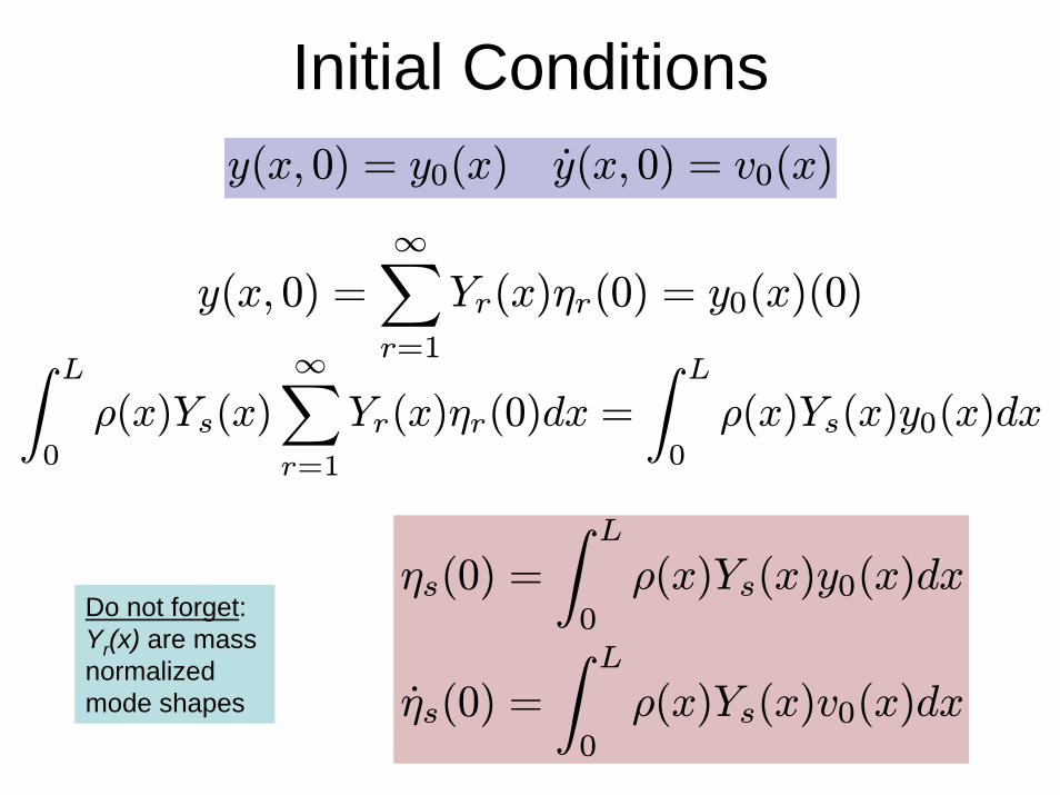
Initial Conditionsy(x, 0) = y0(x) y(x, 0) = v0(x)
y(x, 0) =∞Xr=1
Yr(x)ηr(0) = y0(x)(0)Z L
0
ρ(x)Ys(x)∞Xr=1
Yr(x)ηr(0)dx =
Z L
0
ρ(x)Ys(x)y0(x)dx
ηs(0) =
Z L
0
ρ(x)Ys(x)y0(x)dx
ηs(0) =
Z L
0
ρ(x)Ys(x)v0(x)dx
Do not forget:Yr(x) are mass normalizedmode shapes

Exampleρ = 1Kg/m T = 1N L = 1m
Initial Displacement : y0(x)
0.25
0.1
Initial Velocity : v0(x)

ω1 = π rad/s
ω2 = 2 π rad/s
ω3 = 3 π rad/s
ω4 = 4 π rad/s
ω5 = 5 π rad/s

Normalized Mode Shapes & Initial Condition
Yr(x) =√2 sin
rπx
L⎧⎪⎪⎪⎪⎨⎪⎪⎪⎪⎩η1(0)η2(0)η3(0)η4(0)η5(0)
⎫⎪⎪⎪⎪⎬⎪⎪⎪⎪⎭ =⎧⎪⎪⎪⎪⎨⎪⎪⎪⎪⎩0.05400.01910.00600.0000−0.0022
⎫⎪⎪⎪⎪⎬⎪⎪⎪⎪⎭

0 0.2 0.4 0.6 0.8 1-0.05
0
0.05
0.1
0.15
x
y 0 (x)
Initial DisplacementModal ApproximationMode 1Mode 2Mode 3Mode 4Mode 5

0 0.2 0.4 0.6 0.8 1
-0.1
-0.05
0
0.05
0.1
0.15
x
y(x,
t)Exactt = 0.00 st = 0.25 st = 0.50 st = 0.75 st = 1.00 s

Forced Response
ρ(x)∂2y(x, t)
∂t2− ∂
∂x
∙T (x)
∂y(x, t)
∂x
¸= f(x, t)
y(0, t) = 0 y(L, t) = 0
y(x, 0) = y0(x) y(x, 0) = v0(x)
y(x, t) =∞Xr=1
Yr(x)ηr(t)Yr(x) are mass normalizedmode shapes
∞Xr=1
ρ(x)Yr(x)d2ηr(t)
dt2−∞Xr=1
d
dx
∙T (x)
dYr(x)
dx
¸ηr(t) = f(x, t)
BCs Identically Satisfied : Y (0) ≡ 0 Y (L) ≡ 0

Uncoupled Modal Equations
• Multiply by Ys(x)• Integrate over 0 to LZ L
0
Ys(x)
∞Xr=1
ρ(x)Yr(x)ηr(t)dx−Z L
0
Ys(x)
∞Xr=1
d
dx
∙T (x)
dYr(x)
dx
¸ηr(t)dx
=
Z L
0
Ys(x)f(x, t)dx
ηs(t) + ω2sηs(t) = Ns(t)
Ns(t) =
Z L
0
Ys(x)f(x, t)dx
Do not forget:Yr(x) are mass normalizedmode shapes

Initial Conditionsy(x, 0) = y0(x) y(x, 0) = v0(x)
y(x, 0) =∞Xr=1
Yr(x)ηr(0) = y0(x)(0)Z L
0
ρ(x)Ys(x)∞Xr=1
Yr(x)ηr(0)dx =
Z L
0
ρ(x)Ys(x)y0(x)dx
ηs(0) =
Z L
0
ρ(x)Ys(x)y0(x)dx
ηs(0) =
Z L
0
ρ(x)Ys(x)v0(x)dx
Do not forget:Yr(x) are mass normalizedmode shapes

Steady-State Harmonic Response
f(x, t) = f(x) cosωt
ηs(t) =Ns
ω2s − ω2cosωt
Ns(t) = Ns cosωt where Ns =
Z L
0
Ys(x)f(x)dx
y(x, t) = y(x) cosωt =∞Xr=1
Yr(x)ηr(t)
y(x) =∞Xr=1
Yr(x)Nr
ω2r − ω2=∞Xr=1
Yr(x)
ω2r − ω2Z L
0
Yr(x)f(x)dx

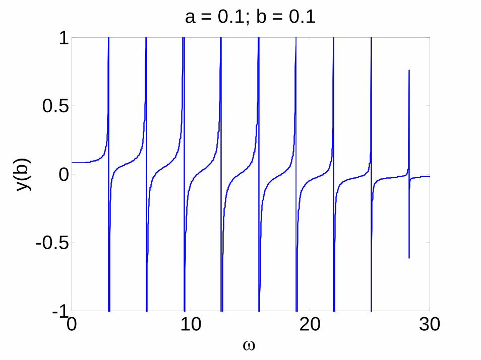
Point Force • Force at a point a
• Displacement at a point b
• Reciprocal Theorem
F=F cos(ωt)ab
Ns =
Z L
0
Ys(x)Fδ(a)dx = FYs(a)
y(b) = F∞Xr=1
Yr(b)Yr(a)
ω2r − ω2
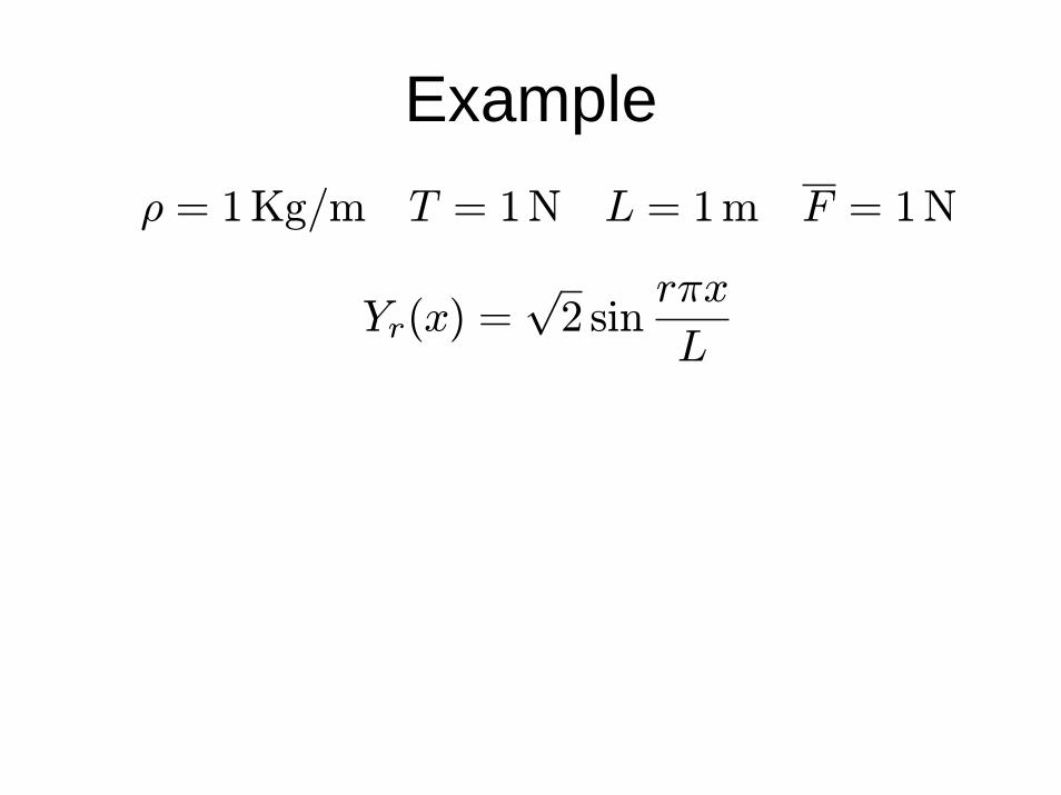
Exampleρ = 1Kg/m T = 1N L = 1m F = 1N
Yr(x) =√2 sin
rπx
L

0 10 20 30-1
-0.5
0
0.5
1
ω
y(b)a = 0.5; b = 0.5

0 10 20 30-1
-0.5
0
0.5
1
ω
y(b)
a = 0.5; b = 0.33333
0 10 20 30-1
-0.5
0
0.5
1
ω
y(b)a = 0.1; b = 0.1

Similar Problem: Axial Vibrationsf(x, t)
m(x), EA(x) u(x, t)
f(x, t)dx
P (x, t) P (x, t) + ∂P (x,t)∂x dx
m(x)dx
P (x, t) = σA = EA² = EA∂u(x,t)∂x

∙P (x, t) +
∂P (x, t)
∂xdx
¸+ f(x, t)dx− P (x, t) = m(x)dx∂
2u(x, t)
∂t2
∂P (x, t)
∂x+ f(x, t) =m(x)
∂2u(x, t)
∂t2
u(0, t) = 0 P (L, t) = EA(x)∂u(x, t)
∂x
¯x=L
= 0
∂
∂x
∙EA(x)
∂u(x, t)
∂x
¸+ f(x, t) = m(x)
∂2u(x, t)
∂t2

Free Vibration
u(0, t) = 0 P (L, t) = EA(x)∂u(x, t)
∂x
¯x=L
∂
∂x
∙EA(x)
∂u(x, t)
∂x
¸= m(x)
∂2u(x, t)
∂t2
u(x, t) = U(x)F (t)
d
dx
∙EA(x)
dU(x)
dxF (t)
¸=m(x)U(x)
d2F (t)
dt2
U(0) = 0dU(x)
dx
¯x=L
= 0

1
m(x)U(x)
d
dx
∙EA(x)
dU(x)
dx
¸=
1
F (t)
d2F (t)
dt2= −ω2
d2F (t)
dt2+ ω2F (t) = 0
⇒ F (t) = A sinωt+B cosωt = C cos(ωt+ φ)
d
dx
∙EA(x)
dU(x)
dx
¸=− ω2m(x)U(x)
U(0) = 0dU(x)
dx
¯x=L
= 0

• For constant mass distribution and cross-sectional stiffness
d
dx
∙EA(x)
dU(x)
dx
¸=− ω2m(x)U(x)
U(0) = 0dU(x)
dx
¯x=L
= 0
d2U(x)
dx2+ω2m
EAU(x) = 0
d2U(x)
dx2+ β2U(x) =0 β2 =
ω2m
EA
U(0) = 0dU(x)
dx
¯x=L
= 0

Fixed-Free
Solution : U(x) = A sinβx+B cosβx
⇒ βrL =
µr − 1
2
¶π, r = 1, 2, · · ·
BCs : U (0) = B = 0dU (x)
dx
¯x=L
= Aβ cos βL = 0¯
⇒ Ur(x) = Ar sin
¡r − 1
2
¢πx
L
ωr =
µr − 1
2
¶π
rEA
mL2⇒ , r = 1, 2, · · ·
, r = 1, 2, · · ·

Fixed-Fixed
Solution : U(x) = A sinβx+B cosβx
BCs : U (0) = B = 0 U (L) = A sin βL = 0
⇒ βrL = rπ, r = 1, 2, · · ·
ωr = rπ
rEA
mL2⇒ , r = 1, 2, · · ·
Ur(x) = Ar sinrπx
L, r⇒ = 1, 2, · · ·

Similar Problem: Torsional Vibrations
θ(x, t)I(x), GJ(x)
τ(x, t)
τ(x, t)dx
T (x, t) + ∂T (x,t)∂x dxT (x, t)
I(x)dx
T (x, t) = GJ(x)∂θ(x,t)∂x
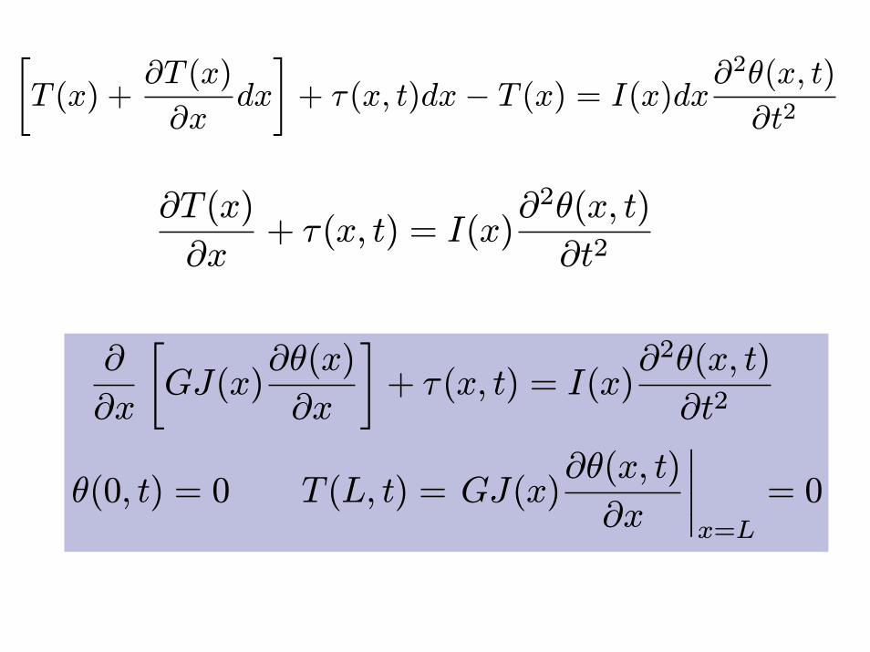
∙T (x) +
∂T (x)
∂xdx
¸+ τ (x, t)dx − T (x) = I(x)dx∂
2θ(x, t)
∂t2
∂T (x)
∂x+ τ(x, t) = I(x)
∂2θ(x, t)
∂t2
∂
∂x
∙GJ(x)
∂θ(x)
∂x
¸+ τ(x, t) = I(x)
∂2θ(x, t)
∂t2
θ(0, t) = 0 T (L, t) = GJ(x)∂θ(x, t)
∂x
¯x=L
= 0


![EIGENVECTORS, EIGENVALUES, AND FINITE STRAIN · unit vector, λ is the length of ... E Eigenvectors have corresponding eigenvalues, and vice-versa F In Matlab, [v,d] = eig(A),](https://img.pdfslide.tips/doc/110x75/5b32041f7f8b9aed688bb633/eigenvectors-eigenvalues-and-finite-strain-unit-vector-is-the-length-of.jpg)