Embed Size (px)
Citation preview
Université de Montréal
Structures algébriques, systèmes superintégrables et
polynômes orthogonaux
par
Vincent Genest
Département de physique
Faculté des arts et des sciences
Thèse présentée à la Faculté des études supérieures
en vue de l’obtention du grade de
Philosophiæ Doctor (PhD) en physique
19 mai 2015
©Vincent Genest, 2015
Université de Montréal
Faculté des études supérieures
Cette thèse intitulée
Structures algébriques, systèmes superintégrables
et polynômes orthogonaux
présentée par
Vincent Genest
a été évaluée par un jury composé des personnes suivantes:
Richard MacKenziePrésident-rapporteur
Luc VinetDirecteur de recherche
Yvan Saint-AubinMembre du jury
Nicolai ReshetikhinExaminateur externe
Thèse acceptée le :
8 juin 2015
Résumé
Cette thèse est divisée en cinq parties portant sur les thèmes suivants: l’interprétation
physique et algébrique de familles de fonctions orthogonales multivariées et leurs applica-
tions, les systèmes quantiques superintégrables en deux et trois dimensions faisant inter-
venir des opérateurs de réflexion, la caractérisation de familles de polynômes orthogonaux
appartenant au tableau de Bannai–Ito et l’examen des structures algébriques qui leurs
sont associées, l’étude de la relation entre le recouplage de représentations irréductibles
d’algèbres et de superalgèbres et les systèmes superintégrables, ainsi que l’interprétation
algébrique de familles de polynômes multi-orthogonaux matriciels.
Dans la première partie, on développe l’interprétation physico-algébrique des familles
de polynômes orthogonaux multivariés de Krawtchouk, de Meixner et de Charlier en tant
qu’éléments de matrice des représentations unitaires des groupes SO(d+1), SO(d,1) et
E(d) sur les états d’oscillateurs. On détermine les amplitudes de transition entre les états
de l’oscillateur singulier associés aux bases cartésienne et polysphérique en termes des
polynômes multivariés de Hahn. On examine les coefficients 9 j de su(1,1) par le biais
du système superintégrable générique sur la 3-sphère. On caractérise les polynômes de
q-Krawtchouk comme éléments de matrices des « q-rotations » de Uq(sl2). On conçoit
un réseau de spin bidimensionnel qui permet le transfert parfait d’états quantiques à
l’aide des polynômes de Krawtchouk à deux variables et on construit un modèle discret
de l’oscillateur quantique dans le plan à l’aide des polynômes de Meixner bivariés.
Dans la seconde partie, on étudie les systèmes superintégrables de type Dunkl, qui
font intervenir des opérateurs de réflexion. On examine l’oscillateur de Dunkl en deux et
trois dimensions, l’oscillateur singulier de Dunkl dans le plan et le système générique sur
la 2-sphère avec réflexions. On démontre la superintégrabilité de chacun de ces systèmes.
On obtient leurs constantes du mouvement, on détermine leurs algèbres de symétrie et
leurs représentations, on donne leurs solutions exactes et on détaille leurs liens avec les
polynômes orthogonaux du tableau de Bannai–Ito.
iii
Dans la troisième partie, on caractérise deux familles de polynômes du tableau de
Bannai–Ito: les polynômes de Bannai–Ito complémentaires et les polynômes de Chihara.
On montre également que les polynômes de Bannai–Ito sont les coefficients de Racah de
la superalgèbre osp(1|2). On détermine l’algèbre de symétrie des polynômes duaux −1
de Hahn dans le cadre du problème de Clebsch-Gordan de osp(1|2). On propose une q-
généralisation des polynômes de Bannai–Ito en examinant le problème de Racah pour la
superalgèbre quantique ospq(1|2). Finalement, on montre que la q-algèbre de Bannai–Ito
sert d’algèbre de covariance à ospq(1|2).
Dans la quatrième partie, on détermine le lien entre le recouplage de représenta-
tions des algèbres su(1,1) et osp(1|2) et les systèmes superintégrables du deuxième ordre
avec ou sans réflexions. On étudie également les représentations des algèbres de Racah–
Wilson et de Bannai–Ito. On montre aussi que l’algèbre de Racah–Wilson sert d’algèbre
de covariance quadratique à l’algèbre de Lie sl(2).
Dans la cinquième partie, on construit deux familles explicites de polynômes d-ortho-
gonaux basées sur su(2). On étudie les états cohérents et comprimés de l’oscillateur fini
et on caractérise une famille de polynômes multi-orthogonaux matriciels.
Mot-clefs
• Polynômes orthogonaux
• Systèmes superintégrables
• Algèbres quadratiques
• Tableau de Bannai–Ito
• Opérateurs de Dunkl
iv
Abstract
This thesis is divided into five parts concerned with the following topics: the physical
and algebraic interpretation of families of multivariate orthogonal functions and their
applications, the study of superintegrable quantum systems in two and three dimensions
involving reflection operators, the characterization of families of orthogonal polynomials
of the Bannai-Ito scheme and the study of the algebraic structures associated to them, the
investigation of the relationship between the recoupling of irreducible representations of
algebras and superalgebras and superintegrable systems, as well as the algebraic inter-
pretation of families of matrix multi-orthogonal polynomials.
In the first part, we develop the physical and algebraic interpretation of the Kraw-
tchouk, Meixner and Charlier families of multivariate orthogonal polynomials as matrix
elements of unitary representations of the SO(d+1), SO(d,1) and E(d) groups on oscil-
lator states. We determine the transition amplitudes between the states of the singular
oscillator associated to the Cartesian and polyspherical bases in terms of the multivariate
Hahn polynomials. We examine the 9 j coefficients of su(1,1) through the generic super-
integrable system on the 3-sphere. We characterize the q-Krawtchouk polynomials as
matrix elements of “q-rotations” of Uq(sl2). We show how to design a two-dimensional
spin network that allows perfect state transfer using the two-variable Krawtchouk poly-
nomials and we construct a discrete model of the two-dimensional quantum oscillator
using the two-variable Meixner polynomials.
In the second part, we study superintegrable systems of Dunkl type, which involve
reflections. We examine the Dunkl oscillator in two and three dimensions, the singular
Dunkl oscillator in the plane and the generic system on the 2-sphere with reflections.
We show that each of these systems is superintegrable. We obtain their constants of
motion, we find their symmetry algebras as well as their representations, we give their
exact solutions and we exhibit their relationship with the orthogonal polynomials of the
Bannai–Ito scheme.
v
In the third part, we characterize two families of polynomials belonging to the Bannai–
Ito scheme: the complementary Bannai-Ito polynomials and the Chihara polynomials.
We also show that the Bannai–Ito polynomials arise as Racah coefficients for the osp(1|2)
superalgebra. We determine the symmetry algebra associated with the dual −1 Hahn
polynomials in the context of the Clebsch-Gordan problem for osp(1|2). We introduce
a q-generalization of the Bannai-Ito polynomials by examining the Racah problem for
the quantum superalgebra ospq(1|2). Finally, we show that the q-deformed Bannai-Ito
algebra serves as a covariance algebra for ospq(1|2).
In the fourth part, we determine the relationship between the recoupling of repre-
sentations of the su(1,1) and osp(1|2) algebras and second-order superintegrable systems
with or without reflections. We also study representations of Racah–Wilson and Bannai–
Ito algebras. Moreover, we show that the Racah–Wilson algebra serves as a quadratic
covariance algebra for sl(2).
In the fifth part, we explicitly construct two families of d-orthogonal polynomials
based on su(2). We investigate the squeezed/coherent states of the finite oscillator and
we characterize a family of matrix multi-orthogonal polynomials.
Keywords
• Orthogonal polynomials
• Superintegrable systems
• Quadratic algebras
• Bannai–Ito scheme
• Dunkl operators
vi
Table des matières
Introduction 1
I Polynômes orthogonaux multivariés et applications 7
Introduction 9
1 The multivariate Krawtchouk polynomials as matrix elements of therotation group representations on oscillator states 131.1 Introduction . . . . . . . . . . . . . . . . . . . . . . . . . . . . . . . . . . . 14
1.2 Representations of SO(3) on the quantum states of the harmonic os-
cillator in three dimensions . . . . . . . . . . . . . . . . . . . . . . . . . . 17
1.2.1 The Weyl algebra . . . . . . . . . . . . . . . . . . . . . . . . . . . . 17
1.2.2 The 3D quantum harmonic oscillator . . . . . . . . . . . . . . . . 18
1.2.3 The representations of SO(3)⊂ SU(3) on oscillator states . . . . 19
1.3 The representation matrix elements
as orthogonal polynomials . . . . . . . . . . . . . . . . . . . . . . . . . . 20
1.3.1 Calculation of the amplitude Wi,k;N . . . . . . . . . . . . . . . . . 21
1.3.2 Raising relations . . . . . . . . . . . . . . . . . . . . . . . . . . . . . 22
1.3.3 Orthogonality relation . . . . . . . . . . . . . . . . . . . . . . . . . 22
1.3.4 Lowering relations . . . . . . . . . . . . . . . . . . . . . . . . . . . . 23
1.4 Duality . . . . . . . . . . . . . . . . . . . . . . . . . . . . . . . . . . . . . . 23
1.5 Generating function . . . . . . . . . . . . . . . . . . . . . . . . . . . . . . 24
1.6 Recurrence relations and difference equations . . . . . . . . . . . . . . 27
1.6.1 Recurrence relations . . . . . . . . . . . . . . . . . . . . . . . . . . 27
1.6.2 Difference equations . . . . . . . . . . . . . . . . . . . . . . . . . . 28
1.7 Integral representation . . . . . . . . . . . . . . . . . . . . . . . . . . . . 29
vii
1.8 Rotations in coordinate planes
and univariate Krawtchouk polynomials . . . . . . . . . . . . . . . . . . 30
1.9 The bivariate Krawtchouk-Tratnik
as special cases . . . . . . . . . . . . . . . . . . . . . . . . . . . . . . . . . 33
1.10 Addition formulas . . . . . . . . . . . . . . . . . . . . . . . . . . . . . . . 34
1.10.1 General addition formula . . . . . . . . . . . . . . . . . . . . . . . . 35
1.10.2 The Tratnik expression . . . . . . . . . . . . . . . . . . . . . . . . . 35
1.10.3 Expansion of the general Krawtchouk polynomials
in the Krawtchouk-Tratnik polynomials . . . . . . . . . . . . . . . 36
1.11 Multidimensional case . . . . . . . . . . . . . . . . . . . . . . . . . . . . . 37
1.12 Conclusion . . . . . . . . . . . . . . . . . . . . . . . . . . . . . . . . . . . . 39
1.A Background on multivariate
Krawtchouk polynomials . . . . . . . . . . . . . . . . . . . . . . . . . . . 40
References . . . . . . . . . . . . . . . . . . . . . . . . . . . . . . . . . . . . . . . . 45
2 The multivariate Meixner polynomials as matrix elements of SO(d,1)
representations on oscillator states 49
2.1 Introduction . . . . . . . . . . . . . . . . . . . . . . . . . . . . . . . . . . . 49
2.2 Representations of SO(2,1) on oscillator states . . . . . . . . . . . . . . 51
2.3 The representation matrix elements as orthogonal polynomials . . . . 53
2.3.1 Calculation of W (β)i,k . . . . . . . . . . . . . . . . . . . . . . . . . . . . 54
2.3.2 Raising relations . . . . . . . . . . . . . . . . . . . . . . . . . . . . . 54
2.3.3 Orthogonality Relation . . . . . . . . . . . . . . . . . . . . . . . . . 55
2.3.4 Lowering Relations . . . . . . . . . . . . . . . . . . . . . . . . . . . 56
2.4 Duality . . . . . . . . . . . . . . . . . . . . . . . . . . . . . . . . . . . . . . 56
2.5 Generating function and
hypergeometric expression . . . . . . . . . . . . . . . . . . . . . . . . . . 57
2.5.1 Generating function . . . . . . . . . . . . . . . . . . . . . . . . . . . 57
2.5.2 Hypergeometric expression . . . . . . . . . . . . . . . . . . . . . . 59
2.6 Recurrence relations and difference equations . . . . . . . . . . . . . . 59
2.6.1 Recurrence relations . . . . . . . . . . . . . . . . . . . . . . . . . . 59
2.6.2 Difference equations . . . . . . . . . . . . . . . . . . . . . . . . . . 60
2.7 One-parameter subgroups and univariate Meixner & Krawtchouk
polynomials . . . . . . . . . . . . . . . . . . . . . . . . . . . . . . . . . . . 61
viii

2.7.1 Hyperbolic subgroups: Meixner polynomials . . . . . . . . . . . . 62
2.7.2 Elliptic subgroup: Krawtchouk polynomials . . . . . . . . . . . . 64
2.8 Addition formulas . . . . . . . . . . . . . . . . . . . . . . . . . . . . . . . 65
2.8.1 General addition formula . . . . . . . . . . . . . . . . . . . . . . . . 65
2.8.2 Special case I: product of two hyperbolic elements . . . . . . . . . 65
2.8.3 General case . . . . . . . . . . . . . . . . . . . . . . . . . . . . . . . 66
2.9 Multivariate case . . . . . . . . . . . . . . . . . . . . . . . . . . . . . . . . 67
2.10 Conclusion . . . . . . . . . . . . . . . . . . . . . . . . . . . . . . . . . . . . 70
References . . . . . . . . . . . . . . . . . . . . . . . . . . . . . . . . . . . . . . . . 70
3 The multivariate Charlier polynomials as matrix elements of theEuclidean group representation on oscillator states 73
3.1 Introduction . . . . . . . . . . . . . . . . . . . . . . . . . . . . . . . . . . . 74
3.2 Representation of E(2) on oscillator states . . . . . . . . . . . . . . . . . 75
3.2.1 The Heisenberg-Weyl algebra . . . . . . . . . . . . . . . . . . . . . 75
3.2.2 The two-dimensional isotropic oscillator . . . . . . . . . . . . . . . 76
3.2.3 Representation of E(2) on oscillator states . . . . . . . . . . . . . 77
3.3 The representation matrix elements as orthogonal polynomials . . . . 78
3.3.1 Calculation of W . . . . . . . . . . . . . . . . . . . . . . . . . . . . . 79
3.3.2 Raising relations . . . . . . . . . . . . . . . . . . . . . . . . . . . . . 79
3.3.3 Orthogonality relation . . . . . . . . . . . . . . . . . . . . . . . . . 80
3.3.4 Lowering relations . . . . . . . . . . . . . . . . . . . . . . . . . . . . 80
3.4 Duality . . . . . . . . . . . . . . . . . . . . . . . . . . . . . . . . . . . . . . 81
3.5 Generating function . . . . . . . . . . . . . . . . . . . . . . . . . . . . . . 82
3.6 Explicit expression in hypergeometric series . . . . . . . . . . . . . . . 83
3.7 Recurrence relations and difference equations . . . . . . . . . . . . . . 84
3.7.1 Recurrence relations . . . . . . . . . . . . . . . . . . . . . . . . . . 84
3.7.2 Difference equations . . . . . . . . . . . . . . . . . . . . . . . . . . 85
3.8 Explicit expression in standard
Charlier and Krawtchouk polynomials . . . . . . . . . . . . . . . . . . . 85
3.9 Integral representation . . . . . . . . . . . . . . . . . . . . . . . . . . . . 86
3.10 Charlier polynomials as limits of
Krawtchouk polynomials . . . . . . . . . . . . . . . . . . . . . . . . . . . 87
3.10.1 Bivariate Krawtchouk polynomials . . . . . . . . . . . . . . . . . . 87
ix
3.10.2 Limit of bivariate Krawtchouk polynomials . . . . . . . . . . . . . 88
3.11 Multidimensional case . . . . . . . . . . . . . . . . . . . . . . . . . . . . . 89
3.12 Conclusion . . . . . . . . . . . . . . . . . . . . . . . . . . . . . . . . . . . . 91
References . . . . . . . . . . . . . . . . . . . . . . . . . . . . . . . . . . . . . . . . 92
4 Interbasis expansions for the isotropic 3D harmonic oscillator andbivariate Krawtchouk polynomials 954.1 Introduction . . . . . . . . . . . . . . . . . . . . . . . . . . . . . . . . . . . 95
4.1.1 Three-dimensional isotropic harmonic oscillator . . . . . . . . . . 96
4.1.2 SO(3)⊂ SU(3) and oscillator states . . . . . . . . . . . . . . . . . . 97
4.1.3 Unitary representations of SO(3) and
bivariate Krawtchouk polynomials . . . . . . . . . . . . . . . . . . 98
4.1.4 The main result . . . . . . . . . . . . . . . . . . . . . . . . . . . . . 100
4.1.5 Outline . . . . . . . . . . . . . . . . . . . . . . . . . . . . . . . . . . 102
4.2 The su(1,1) Lie algebra and
the Clebsch-Gordan problem . . . . . . . . . . . . . . . . . . . . . . . . . 102
4.2.1 The su(1,1) algebra and
its positive-discrete series of representations . . . . . . . . . . . . 102
4.2.2 The Clebsch-Gordan problem . . . . . . . . . . . . . . . . . . . . . 103
4.2.3 Explicit expression for the Clebsch-Gordan coefficients . . . . . . 104
4.3 Overlap coefficients for the isotropic 3D harmonic oscillator . . . . . . 106
4.3.1 The Cartesian/polar overlaps . . . . . . . . . . . . . . . . . . . . . 106
4.3.2 The polar/spherical overlaps . . . . . . . . . . . . . . . . . . . . . . 108
4.4 Conclusion . . . . . . . . . . . . . . . . . . . . . . . . . . . . . . . . . . . . 110
References . . . . . . . . . . . . . . . . . . . . . . . . . . . . . . . . . . . . . . . . 112
5 The multivariate Hahn polynomialsand the singular oscillator 1155.1 Introduction . . . . . . . . . . . . . . . . . . . . . . . . . . . . . . . . . . . 115
5.2 The three-dimensional singular oscillator . . . . . . . . . . . . . . . . . 118
5.2.1 Hamiltonian and spectrum . . . . . . . . . . . . . . . . . . . . . . . 118
5.2.2 The Cartesian basis . . . . . . . . . . . . . . . . . . . . . . . . . . . 118
5.2.3 The spherical basis . . . . . . . . . . . . . . . . . . . . . . . . . . . 119
5.2.4 The main object . . . . . . . . . . . . . . . . . . . . . . . . . . . . . 121
5.3 The expansion coefficients as orthogonal polynomials in two variables 122
x
5.3.1 Calculation of W (α1,α2,α3)i,k;N . . . . . . . . . . . . . . . . . . . . . . . . 122
5.3.2 Raising relations . . . . . . . . . . . . . . . . . . . . . . . . . . . . . 123
5.3.3 Orthogonality relation . . . . . . . . . . . . . . . . . . . . . . . . . 125
5.3.4 Lowering relations . . . . . . . . . . . . . . . . . . . . . . . . . . . . 126
5.4 Generating function . . . . . . . . . . . . . . . . . . . . . . . . . . . . . . 128
5.5 Recurrence relations . . . . . . . . . . . . . . . . . . . . . . . . . . . . . . 130
5.5.1 Forward structure relation in the variable i . . . . . . . . . . . . 130
5.5.2 Backward structure relation in the variable i . . . . . . . . . . . 131
5.5.3 Forward and backward structure relations in the variable k . . . 132
5.5.4 Recurrence relations for the polynomials Q(α1,α2,α2)m,n (i,k; N) . . . 133
5.6 Difference equations . . . . . . . . . . . . . . . . . . . . . . . . . . . . . . 134
5.6.1 First difference equation . . . . . . . . . . . . . . . . . . . . . . . . 135
5.6.2 Second difference equation . . . . . . . . . . . . . . . . . . . . . . . 136
5.7 Expression in hypergeometric series . . . . . . . . . . . . . . . . . . . . 137
5.7.1 The cylindrical-polar basis . . . . . . . . . . . . . . . . . . . . . . . 137
5.7.2 The cylindrical/Cartesian expansion . . . . . . . . . . . . . . . . . 138
5.7.3 The spherical/cylindrical expansion . . . . . . . . . . . . . . . . . 139
5.7.4 Explicit expression for Q(α1,α2,α3)m,n (i,k; N) . . . . . . . . . . . . . . . 140
5.8 Algebraic interpretation . . . . . . . . . . . . . . . . . . . . . . . . . . . . 140
5.8.1 Generalized Clebsch-Gordan problem for su(1,1) . . . . . . . . . 141
5.8.2 Connection with the singular oscillator . . . . . . . . . . . . . . . 142
5.9 Multivariate case . . . . . . . . . . . . . . . . . . . . . . . . . . . . . . . . 144
5.9.1 Cartesian and hyperspherical bases . . . . . . . . . . . . . . . . . 144
5.9.2 Interbasis expansion coefficients as orthogonal polynomials . . . 146
5.10 Conclusion . . . . . . . . . . . . . . . . . . . . . . . . . . . . . . . . . . . . 147
5.A A compendium of formulas for
the bivariate Hahn polynomials . . . . . . . . . . . . . . . . . . . . . . . 148
5.A.1 Definition . . . . . . . . . . . . . . . . . . . . . . . . . . . . . . . . . 148
5.A.2 Orthogonality . . . . . . . . . . . . . . . . . . . . . . . . . . . . . . . 148
5.A.3 Recurrence relations . . . . . . . . . . . . . . . . . . . . . . . . . . 149
5.A.4 Difference equations . . . . . . . . . . . . . . . . . . . . . . . . . . 150
5.A.5 Generating Function . . . . . . . . . . . . . . . . . . . . . . . . . . 150
5.A.6 Forward shift operators . . . . . . . . . . . . . . . . . . . . . . . . . 150
5.A.7 Backward shift operators . . . . . . . . . . . . . . . . . . . . . . . . 151
xi
5.A.8 Structure relations . . . . . . . . . . . . . . . . . . . . . . . . . . . 151
5.B Structure relations for Jacobi polynomials . . . . . . . . . . . . . . . . . 152
5.C Structure relations for Laguerre polynomials . . . . . . . . . . . . . . . 153
References . . . . . . . . . . . . . . . . . . . . . . . . . . . . . . . . . . . . . . . . 153
6 The generic superintegrable system on the 3-sphere andthe 9 j symbols of su(1,1) 1576.1 Introduction . . . . . . . . . . . . . . . . . . . . . . . . . . . . . . . . . . . 157
6.2 The 9 j problem for su(1,1)
in the position representation . . . . . . . . . . . . . . . . . . . . . . . . 159
6.2.1 The addition of four representations and the generic system on
S3 . . . . . . . . . . . . . . . . . . . . . . . . . . . . . . . . . . . . . . 160
6.2.2 The 9 jsymbols . . . . . . . . . . . . . . . . . . . . . . . . . . . . . . 162
6.2.3 The canonical bases by separation of variables . . . . . . . . . . . 163
6.2.4 9 j symbols as overlap coefficients, integral representation and
symmetries . . . . . . . . . . . . . . . . . . . . . . . . . . . . . . . . 166
6.3 Double integral formula and
the vacuum 9 j coefficients . . . . . . . . . . . . . . . . . . . . . . . . . . 167
6.3.1 Extension of the wavefunctions . . . . . . . . . . . . . . . . . . . . 168
6.3.2 The vacuum 9 j coefficients . . . . . . . . . . . . . . . . . . . . . . . 169
6.4 Raising, lowering operators and
contiguity relations . . . . . . . . . . . . . . . . . . . . . . . . . . . . . . . 171
6.4.1 Raising, lowering operators and factorization . . . . . . . . . . . 171
6.4.2 Contiguity relations . . . . . . . . . . . . . . . . . . . . . . . . . . . 172
6.4.3 9 j symbols and rational functions . . . . . . . . . . . . . . . . . . 176
6.5 Difference equations and recurrence relations . . . . . . . . . . . . . . 178
6.6 Conclusion . . . . . . . . . . . . . . . . . . . . . . . . . . . . . . . . . . . . 182
6.A Properties of Jacobi polynomials . . . . . . . . . . . . . . . . . . . . . . . 183
6.B Action of A(α1,α2)− on Ξ(α1,α2,α3,α4)x,y;N . . . . . . . . . . . . . . . . . . . . . . . 184
6.C Action of A(α1−1,α2−1)+ on Ξ(α1,α2,α3,α4)
x,y;N . . . . . . . . . . . . . . . . . . . . 186
References . . . . . . . . . . . . . . . . . . . . . . . . . . . . . . . . . . . . . . . . 188
7 q-Rotations and Krawtchouk polynomials 1937.1 Introduction . . . . . . . . . . . . . . . . . . . . . . . . . . . . . . . . . . . 193
7.2 The Schwinger model for Uq(sl2) and q-rotations . . . . . . . . . . . . 195
xii
7.2.1 Elements of q-analysis . . . . . . . . . . . . . . . . . . . . . . . . . 195
7.2.2 The Schwinger model for Uq(sl2) . . . . . . . . . . . . . . . . . . . 196
7.2.3 Unitary q-rotation operators and matrix elements . . . . . . . . 197
7.3 Matrix elements and self-duality . . . . . . . . . . . . . . . . . . . . . . 199
7.3.1 Matrix elements and quantum q-Krawtchouk polynomials . . . 199
7.3.2 Duality . . . . . . . . . . . . . . . . . . . . . . . . . . . . . . . . . . . 201
7.3.3 The q ↑ 1 limit . . . . . . . . . . . . . . . . . . . . . . . . . . . . . . 202
7.4 Structure relations . . . . . . . . . . . . . . . . . . . . . . . . . . . . . . . 202
7.4.1 Backward relation . . . . . . . . . . . . . . . . . . . . . . . . . . . . 202
7.4.2 Forward relation . . . . . . . . . . . . . . . . . . . . . . . . . . . . . 203
7.4.3 Dual backward and forward relations . . . . . . . . . . . . . . . . 204
7.5 Generating function . . . . . . . . . . . . . . . . . . . . . . . . . . . . . . 204
7.5.1 Generating function with respect to the degrees . . . . . . . . . . 204
7.5.2 Generating function with respect to the variables . . . . . . . . . 206
7.6 Recurrence relation and difference equation . . . . . . . . . . . . . . . 207
7.6.1 Recurrence relation . . . . . . . . . . . . . . . . . . . . . . . . . . . 207
7.6.2 Difference equation . . . . . . . . . . . . . . . . . . . . . . . . . . . 208
7.7 Duality relation with affine
q-Krawtchouk polynomials . . . . . . . . . . . . . . . . . . . . . . . . . . 209
7.8 Conclusion . . . . . . . . . . . . . . . . . . . . . . . . . . . . . . . . . . . . 211
References . . . . . . . . . . . . . . . . . . . . . . . . . . . . . . . . . . . . . . . . 211
8 Spin lattices, state transfer and bivariate Krawtchouk polynomials 215
8.1 Introduction . . . . . . . . . . . . . . . . . . . . . . . . . . . . . . . . . . . 215
8.2 Triangular spin lattices and
one-excitation dynamics . . . . . . . . . . . . . . . . . . . . . . . . . . . . 217
8.3 Representations of O(3) on oscillator states and orthogonal polynomials 218
8.3.1 Calculation of Ws,t;N . . . . . . . . . . . . . . . . . . . . . . . . . . . 219
8.3.2 Raising relations . . . . . . . . . . . . . . . . . . . . . . . . . . . . . 220
8.3.3 Orthogonality relation . . . . . . . . . . . . . . . . . . . . . . . . . 221
8.4 Recurrence relations and exact solutions
of 1-excitation dynamics . . . . . . . . . . . . . . . . . . . . . . . . . . . . 221
8.5 State transfer . . . . . . . . . . . . . . . . . . . . . . . . . . . . . . . . . . 223
8.6 Conclusion . . . . . . . . . . . . . . . . . . . . . . . . . . . . . . . . . . . . 226
xiii
References . . . . . . . . . . . . . . . . . . . . . . . . . . . . . . . . . . . . . . . . 226
9 A superintegrable discrete oscillator and two-variable Meixner poly-nomials 2299.1 Introduction . . . . . . . . . . . . . . . . . . . . . . . . . . . . . . . . . . . 229
9.2 The two-variable Meixner polynomials . . . . . . . . . . . . . . . . . . . 232
9.3 A discrete and superintegrable Hamiltonian . . . . . . . . . . . . . . . 234
9.4 Continuum limit to the standard oscillator . . . . . . . . . . . . . . . . 236
9.4.1 Continuum limit of the two-variable Meixner polynomials . . . . 237
9.4.2 Continuum limit of the raising/lowering operators . . . . . . . . 240
9.5 Conclusion . . . . . . . . . . . . . . . . . . . . . . . . . . . . . . . . . . . . 241
References . . . . . . . . . . . . . . . . . . . . . . . . . . . . . . . . . . . . . . . . 242
II Systèmes superintégrables avec réflexions 245
Introduction 247
10 The Dunkl oscillator in the plane I : superintegrability, separatedwavefunctions and overlap coefficients 24910.1 Introduction . . . . . . . . . . . . . . . . . . . . . . . . . . . . . . . . . . . 250
10.2 The model and exact solutions . . . . . . . . . . . . . . . . . . . . . . . . 251
10.2.1 Solutions in Cartesian coordinates . . . . . . . . . . . . . . . . . . 252
10.2.2 Solutions in polar coordinates . . . . . . . . . . . . . . . . . . . . . 253
10.2.3 Separation of variables and Jacobi-Dunkl polynomials . . . . . . 256
10.3 Superintegrability . . . . . . . . . . . . . . . . . . . . . . . . . . . . . . . 259
10.3.1 Dynamical algebra and spectrum . . . . . . . . . . . . . . . . . . . 259
10.3.2 Superintegrability and the Schwinger-Dunkl algebra . . . . . . . 260
10.4 Overlap Coefficients . . . . . . . . . . . . . . . . . . . . . . . . . . . . . . 262
10.4.1 Overlap coefficients for sxsy =+1 . . . . . . . . . . . . . . . . . . . 262
10.4.2 Overlap coefficients for sxsy =−1 . . . . . . . . . . . . . . . . . . . 266
10.5 The Schwinger-Dunkl algebra and the Clebsch-Gordan problem . . . 269
10.5.1 sl−1(2) Clebsch–Gordan coefficients and
overlap coefficients . . . . . . . . . . . . . . . . . . . . . . . . . . . 269
10.5.2 Occurrence of the Schwinger-Dunkl algebra . . . . . . . . . . . . 271
10.6 Conclusion . . . . . . . . . . . . . . . . . . . . . . . . . . . . . . . . . . . . 271
xiv
10.A Appendix A . . . . . . . . . . . . . . . . . . . . . . . . . . . . . . . . . . . 272
10.A.1 Formulas for Laguerre polynomials . . . . . . . . . . . . . . . . . 272
10.A.2 Formulas for Jacobi polynomials . . . . . . . . . . . . . . . . . . . 272
10.A.3 Formulas for dual −1 Hahn polynomials . . . . . . . . . . . . . . 272
10.B Appendix B . . . . . . . . . . . . . . . . . . . . . . . . . . . . . . . . . . . 273
References . . . . . . . . . . . . . . . . . . . . . . . . . . . . . . . . . . . . . . . . 274
11 The Dunkl oscillator in the plane II : representations of the symmetryalgebra 279
11.1 Introduction . . . . . . . . . . . . . . . . . . . . . . . . . . . . . . . . . . . 280
11.1.1 Superintegrability . . . . . . . . . . . . . . . . . . . . . . . . . . . . 280
11.1.2 The Dunkl oscillator model . . . . . . . . . . . . . . . . . . . . . . 280
11.1.3 Symmetries of the Dunkl oscillator . . . . . . . . . . . . . . . . . . 281
11.1.4 The main object: the Schwinger-Dunkl algebra sd(2) . . . . . . . 282
11.1.5 Outline . . . . . . . . . . . . . . . . . . . . . . . . . . . . . . . . . . 283
11.2 The Cartesian basis . . . . . . . . . . . . . . . . . . . . . . . . . . . . . . 283
11.3 The circular basis . . . . . . . . . . . . . . . . . . . . . . . . . . . . . . . . 286
11.3.1 Transition matrix from the circular to the Cartesian basis . . . 288
11.3.2 Matrix representation of J2 and spectrum . . . . . . . . . . . . . 289
11.4 Diagonalization of J2: the N even case . . . . . . . . . . . . . . . . . . . 292
11.4.1 The operator Q and its simultaneous eigenvalue equation . . . . 292
11.4.2 Recurrence relations . . . . . . . . . . . . . . . . . . . . . . . . . . 294
11.4.3 Generating function and Heun polynomials . . . . . . . . . . . . . 296
11.4.4 Expansion of Heun polynomials in the
complementary Bannai-Ito polynomials . . . . . . . . . . . . . . . 298
11.4.5 Eigenvectors of J2 . . . . . . . . . . . . . . . . . . . . . . . . . . . . 300
11.4.6 The fully isotropic case . . . . . . . . . . . . . . . . . . . . . . . . . 301
11.5 Diagonalization of J2: the N odd case . . . . . . . . . . . . . . . . . . . 302
11.5.1 The operator Q and its simultaneous eigenvalue equation . . . . 302
11.5.2 Recurrence relations . . . . . . . . . . . . . . . . . . . . . . . . . . 304
11.5.3 Generating functions and Heun polynomials . . . . . . . . . . . . 306
11.5.4 Expansion of Heun polynomials in
complementary Bannai-Ito polynomials . . . . . . . . . . . . . . . 306
11.5.5 Eigenvectors of J2 . . . . . . . . . . . . . . . . . . . . . . . . . . . . 308
xv
11.5.6 The fully isotropic case : −1 Jacobi polynomials . . . . . . . . . . 309
11.6 Representations of sd(2) in the J2 eigenbasis . . . . . . . . . . . . . . . 310
11.6.1 The N odd case . . . . . . . . . . . . . . . . . . . . . . . . . . . . . . 310
11.6.2 The N even case . . . . . . . . . . . . . . . . . . . . . . . . . . . . . 312
11.7 Conclusion . . . . . . . . . . . . . . . . . . . . . . . . . . . . . . . . . . . . 314
References . . . . . . . . . . . . . . . . . . . . . . . . . . . . . . . . . . . . . . . . 314
12 The singular and the 2 : 1 anisotropic Dunkl oscillators in the plane 31712.1 Introduction . . . . . . . . . . . . . . . . . . . . . . . . . . . . . . . . . . . 318
12.2 The singular Dunkl oscillator . . . . . . . . . . . . . . . . . . . . . . . . 320
12.2.1 Hamiltonian, dynamical symmetries and spectrum . . . . . . . . 320
12.2.2 Exact solutions and separation of variables . . . . . . . . . . . . . 323
12.2.3 Integrals of motion and symmetry algebra . . . . . . . . . . . . . 327
12.2.4 Symmetries, separability and the Hahn algebra with involutions 328
12.3 The 2 : 1 anisotropic Dunkl oscillator . . . . . . . . . . . . . . . . . . . . 330
12.3.1 Hamiltonian, dynamical symmetries and spectrum . . . . . . . . 331
12.3.2 Exact solutions and separation of variables . . . . . . . . . . . . . 332
12.3.3 Integrals of motion and symmetry algebra . . . . . . . . . . . . . 333
12.3.4 Special case I . . . . . . . . . . . . . . . . . . . . . . . . . . . . . . . 334
12.3.5 Special case II . . . . . . . . . . . . . . . . . . . . . . . . . . . . . . 336
12.4 Conclusion . . . . . . . . . . . . . . . . . . . . . . . . . . . . . . . . . . . . 337
References . . . . . . . . . . . . . . . . . . . . . . . . . . . . . . . . . . . . . . . . 338
13 The Dunkl oscillator in three dimensions 34313.1 Introduction . . . . . . . . . . . . . . . . . . . . . . . . . . . . . . . . . . . 343
13.1.1 Superintegrability . . . . . . . . . . . . . . . . . . . . . . . . . . . . 344
13.1.2 Dunkl oscillator models in the plane . . . . . . . . . . . . . . . . . 344
13.1.3 The three-dimensional Dunkl oscillator . . . . . . . . . . . . . . . 345
13.1.4 Outline . . . . . . . . . . . . . . . . . . . . . . . . . . . . . . . . . . 346
13.2 Superintegrability . . . . . . . . . . . . . . . . . . . . . . . . . . . . . . . 346
13.2.1 Dynamical algebra and spectrum . . . . . . . . . . . . . . . . . . . 346
13.2.2 Constants of motion and
the Schwinger-Dunkl algebra sd(3) . . . . . . . . . . . . . . . . . . 347
13.2.3 An alternative presentation of sd(3) . . . . . . . . . . . . . . . . . 349
13.3 Separated Solutions: Cartesian, cylindrical and spherical coordinates 350
xvi
13.3.1 Cartesian coordinates . . . . . . . . . . . . . . . . . . . . . . . . . . 350
13.3.2 Cylindrical coordinates . . . . . . . . . . . . . . . . . . . . . . . . . 352
13.3.3 Spherical coordinates . . . . . . . . . . . . . . . . . . . . . . . . . . 354
13.4 Conclusion . . . . . . . . . . . . . . . . . . . . . . . . . . . . . . . . . . . . 356
References . . . . . . . . . . . . . . . . . . . . . . . . . . . . . . . . . . . . . . . . 356
14 The Bannai–Ito algebra and a superintegrable system with reflec-tions on the 2-sphere 359
14.1 Introduction . . . . . . . . . . . . . . . . . . . . . . . . . . . . . . . . . . . 359
14.2 The model on S2, superintegrability and
symmetry algebra . . . . . . . . . . . . . . . . . . . . . . . . . . . . . . . 362
14.2.1 The model on S2 . . . . . . . . . . . . . . . . . . . . . . . . . . . . . 362
14.2.2 Superintegrability . . . . . . . . . . . . . . . . . . . . . . . . . . . . 363
14.2.3 Symmetry algebra . . . . . . . . . . . . . . . . . . . . . . . . . . . . 363
14.3 Exact solution . . . . . . . . . . . . . . . . . . . . . . . . . . . . . . . . . . 365
14.3.1 Standard spherical coordinates . . . . . . . . . . . . . . . . . . . . 365
14.3.2 Alternative spherical coordinates . . . . . . . . . . . . . . . . . . . 367
14.4 Connection with sl−1(2) . . . . . . . . . . . . . . . . . . . . . . . . . . . . 368
14.4.1 sl−1(2) algebra . . . . . . . . . . . . . . . . . . . . . . . . . . . . . . 368
14.4.2 Differential/Difference realization and
the model on the 2-sphere . . . . . . . . . . . . . . . . . . . . . . . 369
14.5 Superintegrable model in the plane
from contraction . . . . . . . . . . . . . . . . . . . . . . . . . . . . . . . . 371
14.5.1 Contraction of the Hamiltonian . . . . . . . . . . . . . . . . . . . . 371
14.5.2 Contraction of the constants of motion . . . . . . . . . . . . . . . . 372
14.6 Conclusion . . . . . . . . . . . . . . . . . . . . . . . . . . . . . . . . . . . . 373
References . . . . . . . . . . . . . . . . . . . . . . . . . . . . . . . . . . . . . . . . 374
15 A Dirac–Dunkl equation on S2
and the Bannai–Ito algebra 377
15.1 Introduction . . . . . . . . . . . . . . . . . . . . . . . . . . . . . . . . . . . 377
15.2 Laplace– and Dirac– Dunkl operators for Z32 . . . . . . . . . . . . . . . 379
15.2.1 Laplace– and Dirac– Dunkl operators in R3 . . . . . . . . . . . . . 379
15.2.2 Laplace– and Dirac– operators on S2 . . . . . . . . . . . . . . . . 381
xvii
15.3 Symmetries of the spherical
Dirac–Dunkl operator . . . . . . . . . . . . . . . . . . . . . . . . . . . . . 383
15.4 Representations of the Bannai–Ito algebra . . . . . . . . . . . . . . . . 384
15.5 Eigenfunctions of the spherical
Dirac–Dunkl operator . . . . . . . . . . . . . . . . . . . . . . . . . . . . . 389
15.5.1 Cauchy-Kovalevskaia map . . . . . . . . . . . . . . . . . . . . . . . 389
15.5.2 A basis for MN(R3) . . . . . . . . . . . . . . . . . . . . . . . . . . . 390
15.5.3 Basis spinors and representations of the Bannai–Ito algebra . . 393
15.5.4 Normalized wavefunctions . . . . . . . . . . . . . . . . . . . . . . . 394
15.5.5 Role of the Bannai–Ito polynomials . . . . . . . . . . . . . . . . . . 395
15.6 Conclusion . . . . . . . . . . . . . . . . . . . . . . . . . . . . . . . . . . . . 395
References . . . . . . . . . . . . . . . . . . . . . . . . . . . . . . . . . . . . . . . . 396
III Tableau de Bannai–Ito etstructures algébriques associées 399
Introduction . . . . . . . . . . . . . . . . . . . . . . . . . . . . . . . . . . . . . . . 401
16 Bispectrality of the Complementary Bannai–Ito polynomials 403
16.1 Introduction . . . . . . . . . . . . . . . . . . . . . . . . . . . . . . . . . . . 403
16.2 Bannai–Ito polynomials . . . . . . . . . . . . . . . . . . . . . . . . . . . . 405
16.3 CBI polynomials . . . . . . . . . . . . . . . . . . . . . . . . . . . . . . . . 407
16.4 Bispectrality of CBI polynomials . . . . . . . . . . . . . . . . . . . . . . 412
16.5 The CBI algebra . . . . . . . . . . . . . . . . . . . . . . . . . . . . . . . . 418
16.6 Three OPs families related
to the CBI polynomials . . . . . . . . . . . . . . . . . . . . . . . . . . . . 422
16.6.1 Dual −1 Hahn polynomials . . . . . . . . . . . . . . . . . . . . . . 422
16.6.2 The symmetric Hahn polynomials . . . . . . . . . . . . . . . . . . 424
16.6.3 Para-Krawtchouk polynomials . . . . . . . . . . . . . . . . . . . . 426
16.7 Conclusion . . . . . . . . . . . . . . . . . . . . . . . . . . . . . . . . . . . . 426
References . . . . . . . . . . . . . . . . . . . . . . . . . . . . . . . . . . . . . . . . 427
17 A “continuous” limit of the Complementary Bannai–Ito polynomials:Chihara polynomials 431
17.1 Introduction . . . . . . . . . . . . . . . . . . . . . . . . . . . . . . . . . . . 432
xviii
17.2 Complementary Bannai–Ito polynomials . . . . . . . . . . . . . . . . . . 434
17.3 A “continuous” limit to Chihara polynomials . . . . . . . . . . . . . . . 437
17.4 Bispectrality of the Chihara polynomials . . . . . . . . . . . . . . . . . 438
17.4.1 Bispectrality . . . . . . . . . . . . . . . . . . . . . . . . . . . . . . . 438
17.4.2 Algebraic Structure . . . . . . . . . . . . . . . . . . . . . . . . . . . 440
17.5 Orthogonality of the Chihara polynomials . . . . . . . . . . . . . . . . . 441
17.5.1 Weight function and Chihara’s method . . . . . . . . . . . . . . . 441
17.5.2 A Pearson-type equation . . . . . . . . . . . . . . . . . . . . . . . . 443
17.6 Chihara polynomials and
Big q and −1 Jacobi polynomials . . . . . . . . . . . . . . . . . . . . . . 444
17.6.1 Chihara polynomials and Big -1 Jacobi polynomials . . . . . . . . 444
17.6.2 Chihara polynomials and Big q-Jacobi polynomials . . . . . . . . 446
17.7 Special cases and limits of Chihara polynomials . . . . . . . . . . . . . 447
17.7.1 Generalized Gegenbauer polynomials . . . . . . . . . . . . . . . . 447
17.7.2 A one-parameter extension
of the generalized Hermite polynomials . . . . . . . . . . . . . . . 448
17.7.3 Generalized Hermite polynomials . . . . . . . . . . . . . . . . . . 450
17.8 Conclusion . . . . . . . . . . . . . . . . . . . . . . . . . . . . . . . . . . . . 451
References . . . . . . . . . . . . . . . . . . . . . . . . . . . . . . . . . . . . . . . . 451
18 The Bannai–Ito polynomials as Racah coefficients of the sl−1(2) alge-bra 45518.1 The sl−1(2) algebra, Bannai-Ito polynomials and Leonard pairs . . . . 457
18.1.1 sl−1(2) essentials . . . . . . . . . . . . . . . . . . . . . . . . . . . . . 457
18.1.2 Bannai-Ito polynomials . . . . . . . . . . . . . . . . . . . . . . . . . 458
18.1.3 Leonard pairs and Askey-Wilson relations . . . . . . . . . . . . . 462
18.2 The Clebsch-Gordan problem . . . . . . . . . . . . . . . . . . . . . . . . . 463
18.3 The Racah problem and Bannai-Ito algebra . . . . . . . . . . . . . . . . 465
18.4 Leonard pair and Racah coefficients . . . . . . . . . . . . . . . . . . . . 468
18.5 The Racah problem for the addition of ordinary oscillators . . . . . . . 470
References . . . . . . . . . . . . . . . . . . . . . . . . . . . . . . . . . . . . . . . . 473
19 The algebra of dual −1 Hahn polynomials andthe Clebsch-Gordan problem of sl−1(2) 47719.1 Introduction . . . . . . . . . . . . . . . . . . . . . . . . . . . . . . . . . . . 477
xix
19.2 sl−1(2) and dual −1 Hahn polynomials . . . . . . . . . . . . . . . . . . . 479
19.2.1 The algebra sl−1(2) . . . . . . . . . . . . . . . . . . . . . . . . . . . 479
19.2.2 Dual −1 Hahn polynomials . . . . . . . . . . . . . . . . . . . . . . 480
19.3 The algebra H of −1 Hahn polynomials . . . . . . . . . . . . . . . . . . 482
19.4 The Clebsch-Gordan problem . . . . . . . . . . . . . . . . . . . . . . . . . 484
19.5 A ”dual” representation of H by pentadiagonal matrices . . . . . . . . 488
19.5.1 N odd . . . . . . . . . . . . . . . . . . . . . . . . . . . . . . . . . . . 489
19.5.2 N even . . . . . . . . . . . . . . . . . . . . . . . . . . . . . . . . . . . 492
19.6 Conclusion . . . . . . . . . . . . . . . . . . . . . . . . . . . . . . . . . . . . 493
References . . . . . . . . . . . . . . . . . . . . . . . . . . . . . . . . . . . . . . . . 494
20 The Bannai–Ito algebra and some applications 49720.1 Introduction . . . . . . . . . . . . . . . . . . . . . . . . . . . . . . . . . . . 497
20.2 The Bannai-Ito algebra . . . . . . . . . . . . . . . . . . . . . . . . . . . . 498
20.3 A realization of the Bannai-Ito algebra with shift and reflections op-
erators . . . . . . . . . . . . . . . . . . . . . . . . . . . . . . . . . . . . . . 499
20.4 The Bannai-Ito polynomials . . . . . . . . . . . . . . . . . . . . . . . . . 500
20.5 The recurrence relation of the BI polynomials
from the BI algebra . . . . . . . . . . . . . . . . . . . . . . . . . . . . . . 502
20.6 The paraboson algebra and sl−1(2) . . . . . . . . . . . . . . . . . . . . . 503
20.6.1 The paraboson algebra . . . . . . . . . . . . . . . . . . . . . . . . . 503
20.6.2 Relation with osp(1|2) . . . . . . . . . . . . . . . . . . . . . . . . . . 504
20.6.3 slq(2) . . . . . . . . . . . . . . . . . . . . . . . . . . . . . . . . . . . . 504
20.6.4 The sl−1(2) algebra as a q →−1 limit of slq(2) . . . . . . . . . . . 505
20.7 Dunkl operators . . . . . . . . . . . . . . . . . . . . . . . . . . . . . . . . 506
20.8 The Racah problem for sl−1(2) and the Bannai-Ito algebra . . . . . . . 506
20.9 A superintegrable model on S2 with Bannai-Ito symmetry . . . . . . . 509
20.10 A Dunkl-Dirac equation on S2 . . . . . . . . . . . . . . . . . . . . . . . . 512
20.11 Conclusion . . . . . . . . . . . . . . . . . . . . . . . . . . . . . . . . . . . . 514
References . . . . . . . . . . . . . . . . . . . . . . . . . . . . . . . . . . . . . . . . 514
21 The quantum superalgebra ospq(1|2) and a q-generalizationof the Bannai–Ito polynomials 51921.1 Introduction . . . . . . . . . . . . . . . . . . . . . . . . . . . . . . . . . . . 519
21.2 The quantum superalgebra ospq(1|2) . . . . . . . . . . . . . . . . . . . . 521
xx
21.2.1 Definition and Casimir operator . . . . . . . . . . . . . . . . . . . 521
21.2.2 Hopf algebraic structure . . . . . . . . . . . . . . . . . . . . . . . . 522
21.2.3 Unitary irreducible ospq(1|2)-modules . . . . . . . . . . . . . . . . 523
21.3 The Racah problem . . . . . . . . . . . . . . . . . . . . . . . . . . . . . . . 524
21.3.1 Outline the problem . . . . . . . . . . . . . . . . . . . . . . . . . . . 524
21.3.2 Main observation: q-deformation of the Bannai–Ito algebra . . . 526
21.3.3 Spectra of the Casimir operators . . . . . . . . . . . . . . . . . . . 527
21.3.4 Representations . . . . . . . . . . . . . . . . . . . . . . . . . . . . . 529
21.3.5 The Racah coefficients of ospq(1|2) as basic orthogonal polyno-
mials . . . . . . . . . . . . . . . . . . . . . . . . . . . . . . . . . . . . 530
21.4 q-analogs of the Bannai–Ito polynomials and
Askey-Wilson polynomials with base p =−q . . . . . . . . . . . . . . . . 532
21.5 The q → 1 limit . . . . . . . . . . . . . . . . . . . . . . . . . . . . . . . . . 534
21.5.1 The q → 1 limit of the Racah problem . . . . . . . . . . . . . . . . 534
21.5.2 q → 1 limit of the q-analogs of the Bannai–Ito polynomials . . . 535
21.6 Conclusion . . . . . . . . . . . . . . . . . . . . . . . . . . . . . . . . . . . . 536
References . . . . . . . . . . . . . . . . . . . . . . . . . . . . . . . . . . . . . . . . 537
22 The equitable presentation of ospq(1|2) and a q-analog of the Bannai–Ito algebra 539
22.1 Introduction . . . . . . . . . . . . . . . . . . . . . . . . . . . . . . . . . . . 539
22.2 The ospq(1|2) algebra and its equitable presentation . . . . . . . . . . 541
22.2.1 Definition of ospq(1|2), the grade involution, and representations 541
22.2.2 The equitable presentation of ospq(1|2) . . . . . . . . . . . . . . . 543
22.2.3 The equitable presentation of slq(2) . . . . . . . . . . . . . . . . . 544
22.3 A q-generalization of the Bannai–Ito algebra and the covariance al-
gebra of ospq(1|2) . . . . . . . . . . . . . . . . . . . . . . . . . . . . . . . . 545
22.3.1 The Bannai–Ito algebra and its q-extension . . . . . . . . . . . . 545
22.3.2 Covariance algebra of ospq(1|2) . . . . . . . . . . . . . . . . . . . . 546
22.4 Conclusion . . . . . . . . . . . . . . . . . . . . . . . . . . . . . . . . . . . . 547
References . . . . . . . . . . . . . . . . . . . . . . . . . . . . . . . . . . . . . . . . 548
xxi

IV Problème de Racah et systèmes superintégrables 551
Introduction 553
23 Superintegrability in two dimensions and the Racah-Wilson algebra 55523.1 Introduction . . . . . . . . . . . . . . . . . . . . . . . . . . . . . . . . . . . 555
23.1.1 The Racah-Wilson algebra . . . . . . . . . . . . . . . . . . . . . . . 556
23.1.2 Superintegrability . . . . . . . . . . . . . . . . . . . . . . . . . . . . 557
23.1.3 The generic 3-parameter system on the 2-sphere . . . . . . . . . 557
23.1.4 The 3-parameter system and Racah polynomials . . . . . . . . . 558
23.1.5 Outline . . . . . . . . . . . . . . . . . . . . . . . . . . . . . . . . . . 559
23.2 Representations of the Racah-Wilson algebra . . . . . . . . . . . . . . . 560
23.2.1 The Racah-Wilson algebra and its ladder property . . . . . . . . 560
23.2.2 Discrete-spectrum and finite-dimensional representations . . . . 561
23.2.3 Racah polynomials . . . . . . . . . . . . . . . . . . . . . . . . . . . . 564
23.2.4 Realization of the Racah algebra . . . . . . . . . . . . . . . . . . . 566
23.3 The Racah problem for su(1,1) and
the Racah-Wilson algebra . . . . . . . . . . . . . . . . . . . . . . . . . . . 568
23.3.1 Racah problem essentials for su(1,1) . . . . . . . . . . . . . . . . . 568
23.3.2 The Racah problem and the Racah-Wilson algebra . . . . . . . . 570
23.3.3 Racah problem for the positive-discrete series . . . . . . . . . . . 571
23.4 The 3-parameter superintegrable system on the 2-sphere and the
su(1,1) Racah problem . . . . . . . . . . . . . . . . . . . . . . . . . . . . . 572
23.5 Conclusion . . . . . . . . . . . . . . . . . . . . . . . . . . . . . . . . . . . . 574
References . . . . . . . . . . . . . . . . . . . . . . . . . . . . . . . . . . . . . . . . 574
24 The equitable Racah algebra from three su(1,1) algebras 57724.1 Introduction . . . . . . . . . . . . . . . . . . . . . . . . . . . . . . . . . . . 577
24.1.1 Racah algebra . . . . . . . . . . . . . . . . . . . . . . . . . . . . . . 578
24.1.2 Equitable presentation of the Racah algebra . . . . . . . . . . . . 579
24.1.3 Outline . . . . . . . . . . . . . . . . . . . . . . . . . . . . . . . . . . 580
24.2 The su(1,1) Racah problem . . . . . . . . . . . . . . . . . . . . . . . . . . 580
24.2.1 Positive-discrete series representations and Bargmann realiza-
tion of su(1,1) . . . . . . . . . . . . . . . . . . . . . . . . . . . . . . . 580
24.2.2 Addition schemes for three su(1,1) algebras . . . . . . . . . . . . 581
xxii
24.2.3 6 j-symbols . . . . . . . . . . . . . . . . . . . . . . . . . . . . . . . . 582
24.3 The Racah algebra and the Racah problem . . . . . . . . . . . . . . . . 583
24.3.1 Racah Algebra . . . . . . . . . . . . . . . . . . . . . . . . . . . . . . 583
24.3.2 Z3-symmetric presentation of the Racah problem . . . . . . . . . 584
24.4 Sturm–Liouville model for the Racah algebra . . . . . . . . . . . . . . . 584
24.4.1 Racah problem in the Bargmann picture . . . . . . . . . . . . . . 584
24.4.2 One-variable realization of the Racah algebra and equitable
presentation . . . . . . . . . . . . . . . . . . . . . . . . . . . . . . . 586
24.5 The Racah algebra and the equitable su(2) algebra . . . . . . . . . . . 587
24.5.1 Equitable presentation of the su(2) algebra . . . . . . . . . . . . . 587
24.5.2 Equitable Racah operators from equitable su(2) generators . . . 588
24.5.3 Racah algebra representations from su(2) modules . . . . . . . . 589
24.6 Conclusion . . . . . . . . . . . . . . . . . . . . . . . . . . . . . . . . . . . . 590
References . . . . . . . . . . . . . . . . . . . . . . . . . . . . . . . . . . . . . . . . 591
25 The Racah algebra and superintegrable models 593
25.1 Introduction . . . . . . . . . . . . . . . . . . . . . . . . . . . . . . . . . . . 593
25.1.1 Superintegrable models . . . . . . . . . . . . . . . . . . . . . . . . . 593
25.1.2 Second-order S.I. systems in 2D . . . . . . . . . . . . . . . . . . . . 594
25.1.3 Objectives . . . . . . . . . . . . . . . . . . . . . . . . . . . . . . . . . 595
25.2 Warming up with a simple model . . . . . . . . . . . . . . . . . . . . . . 596
25.3 The Racah algebra . . . . . . . . . . . . . . . . . . . . . . . . . . . . . . . 598
25.4 Representations of the Racah algebra and Racah polynomials . . . . . 599
25.4.1 Racah polynomials . . . . . . . . . . . . . . . . . . . . . . . . . . . . 600
25.4.2 Finite-dimensional representations . . . . . . . . . . . . . . . . . 601
25.4.3 Connection with Racah polynomials . . . . . . . . . . . . . . . . . 603
25.4.4 The Racah algebra from the Racah polynomials . . . . . . . . . . 604
25.5 The generic superintegrable model on S2 and
su(1,1) . . . . . . . . . . . . . . . . . . . . . . . . . . . . . . . . . . . . . . 606
25.6 The Racah problem for su(1,1) and
the Racah algebra . . . . . . . . . . . . . . . . . . . . . . . . . . . . . . . 608
25.7 Conclusion . . . . . . . . . . . . . . . . . . . . . . . . . . . . . . . . . . . . 610
References . . . . . . . . . . . . . . . . . . . . . . . . . . . . . . . . . . . . . . . . 611
xxiii
26 A Laplace-Dunkl equation on S2 and the Bannai–Ito algebra 613
26.1 Introduction . . . . . . . . . . . . . . . . . . . . . . . . . . . . . . . . . . . 613
26.1.1 The Z32 Dunkl-Laplacian on S2 . . . . . . . . . . . . . . . . . . . . 614
26.1.2 The Hopf algebra sl−1(2) . . . . . . . . . . . . . . . . . . . . . . . . 615
26.1.3 The Bannai–Ito algebra and polynomials . . . . . . . . . . . . . . 615
26.1.4 Outline . . . . . . . . . . . . . . . . . . . . . . . . . . . . . . . . . . 617
26.2 Racah problem of sl−1(2) and ∆S2 . . . . . . . . . . . . . . . . . . . . . . 617
26.2.1 Representations of the positive-discrete series and their real-
ization in terms of Dunkl operators . . . . . . . . . . . . . . . . . . 617
26.2.2 The Racah problem, Casimir operators and ∆S2 . . . . . . . . . . 618
26.2.3 Spectrum of ∆S2 from the Racah problem . . . . . . . . . . . . . . 620
26.3 Commutant of ∆S2 and the Bannai–Ito algebra . . . . . . . . . . . . . . 622
26.3.1 Commutant of ∆S2 and symmetry algebra . . . . . . . . . . . . . 622
26.3.2 Irreducible modules of the Bannai–Ito algebra . . . . . . . . . . . 624
26.4 S2 basis functions for irreducible
Bannai–Ito modules . . . . . . . . . . . . . . . . . . . . . . . . . . . . . . 626
26.4.1 Harmonics for ∆S2 . . . . . . . . . . . . . . . . . . . . . . . . . . . . 626
26.4.2 S2 basis functions for BI representations . . . . . . . . . . . . . . 627
26.4.3 Bannai–Ito polynomials as overlap coefficients . . . . . . . . . . . 629
26.5 Conclusion . . . . . . . . . . . . . . . . . . . . . . . . . . . . . . . . . . . . 631
References . . . . . . . . . . . . . . . . . . . . . . . . . . . . . . . . . . . . . . . . 631
V Polynômes multi-orthogonaux matricielset applications 635
Introduction 637
27 d-Orthogonal polynomials and su(2) 639
27.1 Introduction . . . . . . . . . . . . . . . . . . . . . . . . . . . . . . . . . . . 639
27.1.1 d-Orthogonal polynomials . . . . . . . . . . . . . . . . . . . . . . . 640
27.1.2 d-Orthogonal polynomials as
generalized hypergeometric functions . . . . . . . . . . . . . . . . 640
27.1.3 Purpose and outline . . . . . . . . . . . . . . . . . . . . . . . . . . . 641
27.2 The algebra su(2), matrix elements and orthogonal polynomials . . . . 642
xxiv
27.2.1 su(2) essentials . . . . . . . . . . . . . . . . . . . . . . . . . . . . . . 642
27.2.2 Operators and their matrix elements . . . . . . . . . . . . . . . . 644
27.3 Characterization of the A(q)j (`) family . . . . . . . . . . . . . . . . . . . 647
27.3.1 Properties . . . . . . . . . . . . . . . . . . . . . . . . . . . . . . . . . 647
27.3.2 Contractions . . . . . . . . . . . . . . . . . . . . . . . . . . . . . . . 653
27.4 Characterization of the Bn(k) family . . . . . . . . . . . . . . . . . . . . 655
27.4.1 Properties . . . . . . . . . . . . . . . . . . . . . . . . . . . . . . . . . 655
27.4.2 Contractions . . . . . . . . . . . . . . . . . . . . . . . . . . . . . . . 659
27.5 Conclusion . . . . . . . . . . . . . . . . . . . . . . . . . . . . . . . . . . . . 660
References . . . . . . . . . . . . . . . . . . . . . . . . . . . . . . . . . . . . . . . . 662
28 Generalized squeezed-coherent states of the finite one-dimensionaloscillator and matrix multi-orthogonality 66528.1 Introduction . . . . . . . . . . . . . . . . . . . . . . . . . . . . . . . . . . . 666
28.1.1 Finite oscillator and u(2) algebra . . . . . . . . . . . . . . . . . . . 666
28.1.2 Contraction to the standard oscillator . . . . . . . . . . . . . . . . 668
28.1.3 Exponential operator and generalized coherent states . . . . . . 668
28.1.4 Matrix multi-orthogonality . . . . . . . . . . . . . . . . . . . . . . . 669
28.1.5 Outline . . . . . . . . . . . . . . . . . . . . . . . . . . . . . . . . . . 671
28.2 Recurrence relation . . . . . . . . . . . . . . . . . . . . . . . . . . . . . . 671
28.3 Decomposition of matrix elements . . . . . . . . . . . . . . . . . . . . . . 673
28.3.1 The matrix elements λk,m and Krawtchouk polynomials . . . . . 673
28.3.2 The matrix elements φm,n
and vector orthogonal polynomials . . . . . . . . . . . . . . . . . . 674
28.3.3 Full matrix elements and squeezed-coherent states . . . . . . . . 676
28.4 Biorthogonality relation . . . . . . . . . . . . . . . . . . . . . . . . . . . . 677
28.5 Matrix Orthogonality functionals . . . . . . . . . . . . . . . . . . . . . . 678
28.6 Difference equation . . . . . . . . . . . . . . . . . . . . . . . . . . . . . . 679
28.7 Generating functions and ladder relations . . . . . . . . . . . . . . . . . 680
28.8 Observables in the squeezed-coherent states . . . . . . . . . . . . . . . 681
28.9 Contraction to the standard oscillator . . . . . . . . . . . . . . . . . . . 682
28.10 Conclusion . . . . . . . . . . . . . . . . . . . . . . . . . . . . . . . . . . . . 683
References . . . . . . . . . . . . . . . . . . . . . . . . . . . . . . . . . . . . . . . . 684
Conclusion 687
xxv

Bibliographie 691
xxvi
Liste des figures
1 Interactions entre les modèles exactement résolubles, les symétries,
les structures algébriques et les fonctions spéciales . . . . . . . . . . . . 2
8.1 Uniform two-dimensional lattice of triangular shape . . . . . . . . . . . 217
9.1 Wavefunction amplitudes for ξ= 0.8, ψ= 0.8, φ=π/4 and β= 15 . . . . 236
9.2 Wavefunction amplitudes for ξ= 0.8, ψ= 0.8, φ=π/4 and β= 28 . . . . 237
9.3 Wavefunction amplitudes for ξ= 0.5, ψ= 0.8, φ=π/4 and β= 15. . . . . 238
9.4 Wavefunction amplitudes for ξ= 0.8, ψ= 0.8, φ= 0 and β= 15. . . . . . 239
28.1 Squeezing parameter Z2~nz
for r = 2,4,6 (decreasing amplitudes) with
ρ = 0.8 and N = 40. . . . . . . . . . . . . . . . . . . . . . . . . . . . . . . . . 682
xxvii

xxviii

Remerciements
Mes premiers remerciements vont à Luc. Travailler sous sa supervision a été un grand
privilège et même les mots les plus élogieux ne peuvent rendre justice à ses qualités de
superviseur, tant au plan scientifique qu’au plan humain. Je remercie immensément mon
père Christian à qui je dois beaucoup à la fois personnellement et professionnellement. Je
remercie également ma mère Christine pour son éternel support à la fois fort et discret.
Je remercie mes coauteurs, par ordre d’importance: Alexei Zhedanov, Hendrik De Bie,
Mourad Ismail, Hiroshi Miki, Sarah Post et Guo-Fu Yu. Un merci très spécial à Casey.
Un merci à Johanna, pour ses conseils et ses encouragements. Je veux aussi remercier
chaleureusement tous les membres de ma famille et de ma belle famille; l’espace manque
pour expliquer l’apport de chacun d’entre vous. Un remerciement final à mes amis, sur
qui je peux toujours compter.
xxix

xxx
Introduction
L’étude des modèles exactement résolubles joue un rôle fondamental dans l’élaboration
des théories qui visent à décrire et expliquer les phénomènes naturels. De manière
générique, un modèle est dit exactement résoluble s’il est possible d’en exprimer mathé-
matiquement les quantités d’intérêts de manière explicite. Cette notion prend des formes
diverses selon le cadre de travail. Par exemple, en mécanique classique, on dira qu’un sys-
tème formé de deux planètes en interaction gravitationnelle est exactement résoluble car
on peut décrire de manière exacte les trajectoires suivies par chacun des corps [1]. En mé-
canique quantique, le système formé d’un électron et d’un proton (atome d’hydrogène) est
également considéré comme exactement résoluble puisque les énergies possibles du sys-
tème et ses fonctions d’ondes sont explicitement connues, la notion de trajectoire ayant été
évacuée [2]. La notion de résolubilité exacte n’est pas l’apanage de la physique théorique.
Par exemple, en biologie mathématique, le modèle de Moran, qui décrit la dynamique
d’une population de taille constante subissant des mutations aléatoires et dans laquelle
deux types d’allèles se font compétition, est aussi vu comme exactement résoluble car
on peut obtenir de manière explicite la loi de probabilité du nombre individus ayant un
bagage génétique donné [3].
L’importance des modèles exactement résolubles en physique tient à de nombreux élé-
ments; nous en mentionnons quelques-uns. Tout d’abord, ces modèles constituent un outil
de choix dans la validation des principes théoriques fondamentaux. En effet, ils permet-
tent de formuler des prévisions très précises qui peuvent être par la suite soumises à
l’expérimentation. À ce titre, la description de la structure fine de l’atome d’hydrogène
obtenue par le truchement de l’équation de Dirac est éloquente [4]. Ensuite, les mo-
dèles ayant des solutions exactes permettent d’accéder à une compréhension plus fine du
contenu physique des théories qui les sous-tendent car ils permettent l’analyse détaillée
du rôle de tous les paramètres qui y interviennent; c’est d’ailleurs en partie pourquoi
l’examen de ces systèmes occupe une place prépondérante dans les cursus de physique.
1
Un autre élément qui souligne l’importance des systèmes exactement résolubles est que
ceux-ci sont constamment utilisés dans l’élaboration de modèles plus raffinés et dont les
caractéristiques sont étudiées à partir de celles du modèle original, entre autres en uti-
lisant la théorie des perturbations. On peut penser ici aux nombreux systèmes quantiques
basés sur le modèle de l’oscillateur harmonique [2]. Finalement, l’étude des modèles ex-
actement résolubles est un lieu de rencontre privilégié entre la physique théorique et
les mathématiques. Ces deux disciplines se sont à de nombreuses reprises fertilisées
mutuellement par le passé, conduisant à des avancées significatives dans les deux do-
maines. Le théorème de Noether, qui relie les symétries aux lois de conservation en est
un exemple particulièrement pertinent [5].
Les symétries sont le dénominateur commun des modèles exactement résolubles: em-
piriquement, on observe qu’il n’y a de solutions exactes qu’en présence de symétries.
Celles-ci se présentent sous diverses formes et sont décrites mathématiquement par des
structures algébriques variées. Dans bien des cas, les solutions des modèles exacte-
ment résolubles s’expriment en termes de fonctions spéciales. Ces fonctions encodent les
symétries des systèmes dans lesquels elles apparaissent. Un exemple typique est celui de
l’oscillateur quantique en trois dimensions et des harmoniques sphériques. Ce système
est invariant sous les rotations, décrites par le groupe SO(3). L’invariance sous les rota-
tions conduit à la séparation de l’équation de Schrödinger en coordonnées sphériques, les
harmoniques sphériques apparaissent comme solutions exactes à l’équation angulaire et
elles forment une base pour les représentations irréductibles de so(3) [6].
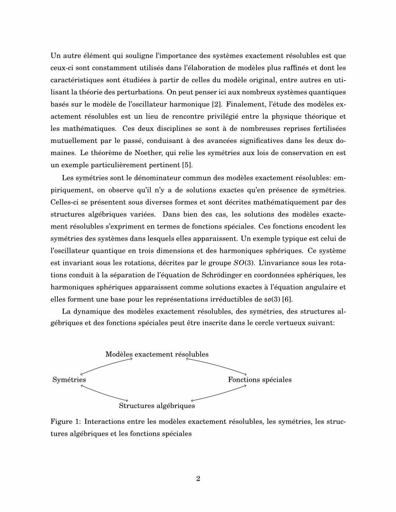
La dynamique des modèles exactement résolubles, des symétries, des structures al-gébriques et des fonctions spéciales peut être inscrite dans le cercle vertueux suivant:
Modèles exactement résolubles
Symétriesvv
22
Fonctions spéciales))
ll
Structures algébriquesrr
55
++
hh
Figure 1: Interactions entre les modèles exactement résolubles, les symétries, les struc-
tures algébriques et les fonctions spéciales
2
Le chemin typique que l’on songe parcourir dans ce schéma est le suivant. On imagine
d’abord un modèle d’intérêt. Ensuite, on trouve les symétries de ce modèle et on détermine
la structure mathématique qui décrit ces symétries. Puis, on construit les représentations
de cette structure algébrique et on établit le lien entre ses représentations et les fonctions
spéciales. Finalement on met à profit les fonctions spéciales pour exprimer les solutions
du modèle et/ou pour en calculer certaines quantités importantes.
Il s’avère toutefois fructueux de prendre comme point de départ n’importe quel som-
met de la figure 1. Par exemple, on peut obtenir et caractériser une nouvelle famille de
fonctions spéciales, déterminer la structure algébrique dont ils encodent les propriétés,
chercher des modèles dont les symétries sont décrites par cette structure et donner les
solutions des modèles obtenus en termes de cette nouvelle famille de fonctions.
Le diagramme 1 reflète l’essence de la recherche qui a mené à la présente thèse, dans
laquelle la résolubilité exacte est recherchée et étudiée par le truchement des symétries,
des structures algébriques et de leurs représentations ainsi que des fonctions spéciales.
La thèse comporte vingt-huit articles qui contribuent à un ou à plusieurs des axes de
recherche qui apparaissent sur le diagramme 1. Les résultats originaux qu’elle contient
sont en nombre. Ils concernent principalement les polynômes orthogonaux (une classe
particulière de fonctions spéciales), les systèmes quantiques superintégrables (une classe
de modèles exactement résolubles) et certaines algèbres et superalgèbres quadratiques
telles que les algèbres de Bannai–Ito et de Racah.
La thèse se divise en cinq parties comprenant chacune une série d’articles sur un
thème commun. Toutes les parties, à l’exception peut-être de la dernière, sont en fort lien
les unes avec les autres via le diagramme 1. En outre, plusieurs articles auraient pu se
retrouver dans une autre partie que celle où ils sont actuellement.
La partie I de la thèse est intitulée Polynômes orthogonaux multivariés et applications.
Dans cette partie, on traite des interprétations physique et algébrique de six familles de
fonctions orthogonales multivariées et on en détaille trois applications physiques. Dans
l’introduction, on explique sommairement le contexte général de l’étude des polynômes
orthogonaux multivariés. Dans les chapitres 1 à 3, on montre comment les familles de
polynômes orthogonaux à d variables de Krawtchouk, Meixner et Charlier interviennent
respectivement en tant qu’éléments de matrice des représentations unitaires des groupes
de rotation SO(d+1), du groupe de Lorentz SO(d,1) et du groupe euclidien E(d) sur les
états de l’oscillateur harmonique [7, 8, 9]. On illustre de quelle façon cette interprétation
conduit à une caractérisation complète de ces familles de polynômes. Dans le chapitre 4,
3
on établit une relation entre les polynômes de Krawtchouk à 2 variables, les coefficients
de Clebsch-Gordan de l’algèbre su(1,1) donnés par les polynômes de Hahn et les coeffi-
cients de transition entre les bases sphérique et cartésienne de l’oscillateur harmonique
en trois dimensions [10]. Dans le chapitre 5, on montre que les polynômes de Hahn à d
variables de Karlin et McGregor interviennent dans les amplitudes de transition entre
les états associés aux bases cartésienne et polysphérique de l’oscillateur singulier en d+1
dimensions [11]. On exploite ensuite cette identification pour donner une caractérisation
complète de ces polynômes. Dans le chapitre 6, on utilise le lien entre le recouplage de n+1
représentations de su(1,1) et le modèle superintégrable générique sur la n-sphère obtenu
dans la partie IV pour étudier les coefficients 9 j de su(1,1); on montre que ces coefficients
sont donnés en termes de fonctions rationnelles orthogonales et on en extrait plusieurs
propriétés [12]. Dans le chapitre 7, on met la table pour l’obtention d’une q-généralisation
de la relation entre les polynômes de Krawtchouk multivariés et les représentations du
groupe des rotations en déterminant le lien entre les polynômes de q-Krawtchouk et les
« q-rotations » dans l’algèbre quantique Uq(sl2) [13]. Dans les chapitres 8 et 9, on présente
deux applications des polynômes orthogonaux multivariés. Premièrement, on explique
comment les polynômes de Krawtchouk à deux variables peuvent être utilisés pour con-
cevoir un réseau de spins à deux dimensions qui permet le transfert parfait d’états quan-
tiques [14]. Deuxièmement, on élabore un modèle discret de l’oscillateur harmonique
quantique en deux dimensions ayant la même algèbre de symétrie su(2) que le modèle
usuel [15].
La partie II de la thèse est intitulée systèmes superintégrables avec réflexions. Dans
cette partie, on étudie une série de systèmes quantiques superintégrables en deux et trois
dimensions dont les hamiltoniens contiennent des opérateurs de réflexion de la forme
Ri f (xi) = f (−xi). Dans l’introduction, on rappelle la notion de superintégrabilité et on
définit les opérateurs de Dunkl. Dans les chapitres 10 et 11, on examine le modèle de
l’oscillateur de Dunkl dans le plan [16, 17]. On montre que ce système est superinté-
grable, on obtient ses constantes du mouvement et on en donne l’algèbre de symétrie et
les solutions exactes. On montre que dans ce modèle les amplitudes de transition entre
les états associés aux bases polaire et cartésienne sont exprimées en termes des coeffi-
cients de Clebsch-Gordan de la superalgèbre de Lie osp(1|2) qui sont donnés en termes
des polynômes duaux −1 de Hahn appartenant au tableau de Bannai–Ito discuté dans
la partie III. On procède aussi à une analyse détaillée des représentations de l’algèbre
de symétrie du modèle, dénommée algèbre de Schwinger–Dunkl. Dans le chapitre 12, on
4
considère une extension du modèle faisant intervenir des termes de potentiel singuliers;
on montre que le système demeure superintégrable, on donne ses constantes du mouve-
ment, son algèbre de symétrie et ses solutions exactes [18]. Dans le chapitre 13, on ex-
amine l’oscillateur de Dunkl en trois dimensions, lui aussi superintégrable et exactement
résoluble [19]. Dans le chapitre 14, on introduit le modèle superintégrable générique
sur la 2-sphère avec réflexions [20]. Grâce aux résultats obtenus dans la partie IV, on
montre que l’hamiltonien de ce système est lié à l’opérateur de Casimir total intervenant
dans la combinaison de trois représentations irréductibles de osp(1|2). On détermine con-
séquemment que l’algèbre de symétrie engendrée par les constantes du mouvement de
ce système est l’algèbre de Bannai–Ito. On montre aussi la contraction de ce système
vers l’oscillateur de Dunkl dans le plan. Finalement, dans le chapitre 15, on examine
l’équation de Dirac–Dunkl sur la 2-sphère [21]. On montre que l’algèbre de symétrie de
cette équation est aussi l’algèbre de Bannai–Ito, on construit les représentations de di-
mension finie de cette algèbre et on construit les solutions exactes du modèle à l’aide de
l’extension de Cauchy–Kovalevskaia.
La partie III s’intitule Tableau de Bannai–Ito et structure algébriques associées. Dans
cette partie, on étudie des familles de polynômes orthogonaux appartenant à la classe des
polynômes de Bannai–Ito et on étudie les structures algébriques associées à ces fonctions.
Dans l’introduction, on rappelle l’origine des polynômes du tableau de Bannai–Ito, aussi
appelés polynômes orthogonaux «−1 », et on explique brièvement la notion de bispectra-
lité. Dans le chapitre 16, on démontre la bispectralité des polynômes complémentaires de
Bannai–Ito, c’est-à-dire qu’on obtient l’opérateur duquel ils sont fonctions propres [22].
Dans le chapitre 17, on introduit et on caractérise une famille de polynômes «−1 » appelés
polynômes de Chihara [23]. Dans le chapitre 18, on montre que les polynômes de Bannai–
Ito interviennent comme coefficients de Racah de la superalgèbre osp(1|2), aussi appelée
sl−1(2) [24]. Dans le chapitre 19, on obtient la structure algébrique qui sous-tend les
polynômes duaux −1 de Hahn et on établit comment cette structure intervient dans le
problème de Clebsch-Gordan de sl−1(2) [25]. Le chapitre 20 est le compte-rendu d’une
conférence de revue sur l’algèbre de Bannai-Ito et ses applications [26]. Dans le chapitre
21, on introduit une q-généralisation des polynômes de Bannai–Ito et de leur algèbre en
considérant les coefficients de Racah de la superalgèbre quantique ospq(1|2) [27]. Dans le
chapitre 22, on établit que la q-algèbre de Bannai–Ito est aussi l’algèbre de covariance de
ospq(1|2) [28].
La partie IV de la thèse s’intitule Problème de Racah et systèmes superintégrables.
5
Dans cette partie, on détermine le lien entre le recouplage de représentations des algèbres
su(1,1) et osp(1|2) et les systèmes superintégrables dont les constantes du mouvement
sont du deuxième ordre. Dans l’introduction on rappelle les bases du problème de Racah,
qui advient lors du recouplage de trois représentations. Dans le chapitre 23, on étudie
les liens entre le problème de Racah pour l’algèbre de Lie su(1,1), l’algèbre de Racah–
Wilson et le système superintégrable générique sur la 2-sphère [29]. Dans le chapitre 24,
on montre que l’algèbre de Racah peut également être vue comme l’algèbre de covariance
quadratique de sl2 [30]. Le chapitre 25 est le compte-rendu d’une conférence de revue
sur l’algèbre de Racah [31]. Finalement, dans le chapitre 26, on établit le lien entre le
problème de Racah pour la superalgèbre osp(1|2), l’algèbre de Bannai–Ito et le système
superintégrable générique sur la 2-sphère avec réflexions [32].
La partie V est intitulée Polynômes multi-orthogonaux et applications. Elle est légère-
ment à la marge des autres parties de la thèse et témoigne de mes premiers travaux. Dans
l’introduction, la notion de d-orthogonalité et de multi-orthogonalité matricielle est re-
vue. Dans le chapitre 27, on définit deux nouvelles familles de polynômes d-orthogonaux
en utilisant les représentations de su(2) [33]. Dans le chapitre 28, on utilise ces résul-
tats pour étudier les états cohérents/comprimés de l’oscillateur fini et pour présenter de
manière explicite une famille de polynômes multi-orthogonaux matriciels [34].
6
Partie I
Polynômes orthogonaux multivariéset applications
7

Introduction
Les polynômes orthogonaux forment une classe particulièrement importante de fonctions
spéciales [35], notamment en raison de leurs nombreuses applications à la physique
mathématique, aux probabilités et aux processus stochastiques, à la théorie de l’approxi-
mation et aux matrices aléatoires. Une suite de polynômes Pn(x)∞n=0, où Pn(x) est un
polynôme de degré n en x, constitue une famille de polynômes orthogonaux s’il existe une
fonctionnelle linéaire L telle que pour tous les entiers non-négatifs m et n, on a [36]
L [Pm(x)Pn(x)]= 0 si m 6= n et L [Pn(x)2] 6= 0.
De tous les polynômes orthogonaux, le sous-ensemble des polynômes orthogonaux hyper-
géométriques est certainement l’un des plus importants [37]. Il est constitué des familles
de polynômes orthogonaux qui peuvent s’écrire de manière explicite en termes de séries ou
de q-séries hypergéométriques. Les séries hypergéométriques, dénotées pFq, sont définies
ainsi [35]
pFq
(a1,a2, . . . ,ap
b1,b2, . . . ,bq
∣∣∣ z)= ∑
k≥0
(a1,a2, . . . ,ap)k
(b1,b2, . . . ,bq)k
zk
k!,
avec (a1,a2, . . . ,ap)k = (a1)k(a2)k · · · (ap)k où (a)k est le symbole de Pochhammer
(a)k =k−1∏i=0
(a+ i) avec (a)0 = 1.
Les q-séries hypergéométriques, généralement dénotées par rφs, sont définies par [38]
rφs
(a1,a2, . . . ,ar
b1,b2, . . . ,bs
∣∣∣ q, z)= ∑
k≥0
(a1,a2, . . . ,ar; q)k
(b1,b2, . . . ,bs; q)k(−1)(1+s−r)kq(1+s−r)(k
2) zk
(q; q)k,
avec (a1,a2, . . . ,ar; q)k = (a1; q)k(a2; q)k · · · (ar; q)k où (a; q)k est le symbole de Pochhammer
q-déformé
(a; q)=k∏
i=1(1−aqi−1) avec (a; q)0 = 1.
9

Les polynômes orthogonaux hypergéométriques sont typiquement organisés au sein d’une
hiérarchie connue sous le nom de Tableau de Askey1 [39]. Au sommet de cette hiérarchie
trônent les polynômes de Askey–Wilson et les q-polynômes de Racah, qui ont chacun cinq
paramètres, incluant q. Tous les polynômes du tableau d’Askey peuvent être obtenus
à partir de ces deux familles par des limites, notamment la limite « classique » q → 1,
ou alors par des choix particuliers de paramètres. Les polynômes du tableau d’Askey
sont ubiquitaires, comme en témoignent les 1500 citations de la monographie de 1998 de
Koekoek, Lesky et Swarttouw [39].
Les polynômes du tableau d’Askey ont presque tous une interprétation algébrique. Ils
sont tantôt éléments de matrices ou vecteurs de base pour certaines représentations irré-
ductibles d’algèbres de Lie de rang 1, tantôt coefficients de Clebsch-Gordan ou de Racah
pour ces mêmes algèbres [40, 41, 42]. Dans tous les cas, les interprétations algébriques
des familles de polynômes orthogonaux permettent d’en déduire un grand nombre de pro-
priétés. En fait, le cadre algébrique est lui-même à l’origine de la découvert de certains
de ces objets, dont les polynômes de Racah, q-Racah, Wilson et Askey–Wilson.
Il est naturel de chercher à généraliser la hiérarchie du tableau d’Askey aux poly-
nômes orthogonaux multivariés. Il faut savoir toutefois que de manière générale, l’étude
des polynômes orthogonaux à plusieurs variables est plus difficile que celle des polynômes
univariés, notamment en raison du fait que dans le cas multivarié la mesure d’ortho-
gonalité ne caractérise pas complètement les polynômes associés [43]. Il n’y pas à ce
jour de théorie unifiée de tous les polynômes orthogonaux multivariés, à l’exception des
polynômes multivariés associés aux systèmes de racines, qui ne sont pas étudiés dans
cette thèse [43]. Cependant, nombreuses sont les familles qui sont connues et bien carac-
térisées.
Les premiers exemples de familles de polynômes multivariés généralisant celles du
tableau de Askey ont été proposés dans un cadre probabiliste au début des années 70.
C’est Robert Griffiths qui a généralisé à plusieurs variables les familles de polynômes de
Krawtchouk et de Meixner en utilisant des fonctions génératrices associées aux distri-
butions multinomiale et multinomiale négative [44, 45]; voir aussi les travaux de Milch
qui précèdent ceux de Griffiths [46]. Les polynômes multivariés de Krawtchouk étudiés
par Griffiths ont par la suite été redécouverts à quelques reprises, notamment dans [47].
Durant la même période, Karlin et McGregor ont généralisé à plusieurs variables les
polynômes de Hahn en considérant le modèle de Moran à plusieurs espèces [48]. On doit
1Notons ici que les polynômes −1, bien qu’hypergéométriques, ne se retrouvent pas dans cette hiérarchie.
10
aussi souligner les nombreux travaux de Koornwinder sur les polynômes à deux variables
[49]. Plusieurs années plus tard, Tratnik a proposé une version multivariée du tableau
d’Askey à q = 1 [50, 51]. Les polynômes multivariés proposés par Tratnik, qui incluent
ceux de Karlin et McGregor, sont construits en combinant de manière non triviale des
polynômes orthogonaux univariés du tableau d’Askey. De nombreux travaux visant la
caractérisation de ces polynômes ont par la suite été publiés [52]. Plus récemment, la
même approche a été reprise par Gasper et Rahman pour définir des q-déformations des
polynômes proposées par Tratnik [53]; ces familles demeurent toutefois relativement peu
étudiées [54].
Cette partie de la thèse porte sur l’interprétation physique et algébrique de certaines
familles de polynômes orthogonaux ainsi que sur certaines de leurs applications concrètes
à la physique. Tout d’abord, on montre que les polynômes de Krawtchouk, de Meixner
(tels que définis par Griffiths) et de Charlier à d-variables correspondent aux éléments de
matrices des représentations unitaires des groupes de Lie SO(d+1), SO(d,1) et E(d) sur
les états de l’oscillateur harmonique. Les résultats qui concernent les groupes SO(d+1)
et E(d) sont directement liés aux propriétés de transformation de systèmes d’oscillateurs
harmoniques sous les rotations et les transformations euclidiennes. On illustre également
le lien entre les polynômes de Krawtchouk à deux variables et les coefficients de tran-
sition entre les états des bases cartésienne et sphérique pour l’oscillateur harmonique
en trois dimensions. On montre aussi que les polynômes de Hahn à d variables de
Karlin et McGregor interviennent dans les amplitudes de transition entre les états des
bases cartésienne et polysphérique de l’oscillateur singulier en d+1 dimensions. On exa-
mine également les coefficients 9 j de su(1,1) par la lorgnette du système superintégrable
générique sur la 3-sphère et on montre que ces coefficients s’expriment non pas en ter-
mes de polynômes, mais en termes de fonctions rationnelles. Par ailleurs, on montre
que les polynômes de q-Krawtchouk interviennent en tant qu’éléments de matrice des
« q-rotations » de l’algèbre quantique Uq(sl2). Les deux applications qui sont présentées
concernent respectivement le transfert parfait d’états quantiques à l’aide de réseaux de
spins et la discrétisation du modèle de l’oscillateur quantique en deux dimensions.
11

12

Chapitre 1
The multivariate Krawtchoukpolynomials as matrix elements of therotation group representations onoscillator states
V. X. Genest, L. Vinet et A. Zhedanov (2013). The multivariate Krawtchouk polynomials
as matrix elements of the rotation group representations on oscillator states. Journal of
Physics A: Mathematical and Theoretical 46 505203
Abstract. An algebraic interpretation of the bivariate Krawtchouk polynomials is pro-
vided in the framework of the 3-dimensional isotropic harmonic oscillator model. These
polynomials in two discrete variables are shown to arise as matrix elements of unitary
reducible representations of the rotation group in 3 dimensions. Many of their properties
are derived by exploiting the group-theoretic setting. The bivariate Tratnik polynomials
of Krawtchouk type are seen to be special cases of the general polynomials that corre-
spond to particular rotations involving only two parameters. It is explained how the
approach generalizes naturally to (d+1) dimensions and allows to interpret multivariate
Krawtchouk polynomials as matrix elements of SO(d+1) unitary representations. Indi-
cations are given on the connection with other algebraic models for these polynomials.
13
1.1 Introduction
The main objective of this article is to offer a group-theoretic interpretation of the mul-
tivariable generalization of the Krawtchouk polynomials and to show how their theory
naturally unfolds from this picture. We shall use as framework the space of states of the
quantum harmonic oscillator in d +1 dimensions. It will be seen that the Krawtchouk
polynomials in d variables arise as matrix elements of the reducible unitary representa-
tions of the rotation group SO(d+1) on the energy eigenspaces of the (d+1)-dimensional
oscillator. For simplicity, we shall focus on the d = 2 case. The bivariate Krawtchouk poly-
nomials will thus appear as matrix elements of SO(3) representations; we will indicate
towards the end of the paper how the results directly generalize to an arbitrary finite
number of variables.
The ordinary Krawtchouk polynomials in one discrete variable have been obtained by
Krawtchouk [19] in 1929 as polynomials orthogonal with respect to the binomial distribu-
tion. They possess many remarkable properties [17, 25] (second-order difference equation,
duality, explicit expression in terms of Gauss hypergeometric function, etc.) and enjoy
numerous applications. The importance of these polynomials in mathematical physics is
due, to a large extent, to the fact that the matrix elements of SU(2) irreducible repre-
sentations known as the Wigner D functions can be expressed in terms of Krawtchouk
polynomials [4, 18].
The determination of the multivariable Krawtchouk polynomials goes back at least
to 1971 when Griffiths obtained [5] polynomials in several variables that are orthogonal
with respect to the multinomial distribution using, in particular, a generating function
method. These polynomials, especially the bivariate ones, were subsequently rediscov-
ered by several authors. For instance, the 2-variable Krawtchouk polynomials appear as
matrix elements of U(3) group representations in [26] and the same polynomials occur as
9 j symbols of the oscillator algebra in [29]. An explicit expression in terms of Gel’fand-
Aomoto generalized hypergeometric series is given in [24]. Interest was sparked in recent
years with the publication by Hoare and Rahman of a paper [11] in which the 2-variable
Krawtchouk polynomials were presented, anew, from a probabilistic perspective. This
led to bivariate Krawtchouk polynomials being sometimes called Rahman polynomials. A
number of papers followed [6, 7, 8, 23]; the approach of [11], related to Markov chains,
was extended to the multivariate case in reference [7] to which the reader is directed for
an account of the developments at that point in time.
14
Germane to the present paper are references [13] and [12]. In the first of these pa-
pers, Iliev and Terwilliger offer a Lie-algebraic interpretation of the bivariate Krawtchouk
polynomials using the algebra sl3(C). In the second paper, this study was extended by
Iliev to the multivariate case by connecting the Krawtchouk polynomials in d variables
to sld+1(C). In these two papers, the Krawtchouk polynomials appear as overlap coef-
ficients between basis elements for two modules of sl3(C) or sld+1(C) in general. The
basis elements for the representation spaces are defined as eigenvectors of two Cartan
subalgebras related by an anti-automorphism specified by the parameters of the poly-
nomials. The interpretation presented here is in a similar spirit. We shall indicate in
Section 5 and in the appendix what are the main observations that are required if one
wishes to establish the correspondence. In essence, the key is in the recognition that the
anti-automorphism used in [12] and [13] can be taken to be a rotation (times i). The anal-
ysis is then brought in the realm of the theory of Lie group representations. This entails
connecting two parametrizations of the polynomials: the one used in the cited literature
and the other that naturally emerges in the interpretation to be presented, in terms of
rotation matrix elements. It is noted that the connection with SO(d+1) rotations readily
explains the d(d+1)/2 parameters of the polynomials.
A major advance in the theory of multivariable orthogonal polynomials was made by
Tratnik [27], who defined a family of multivariate Racah polynomials, thereby obtaining
a generalization to many variables of the discrete polynomials at the top of the Askey
scheme and extending the multivariate Hahn polynomials introduced by Karlin and Mc-
Gregor in [16] in the context of linear growth models with many types. These Racah
polynomials in d variables depend on d +2 parameters; they can be expressed as prod-
ucts of single variable Racah polynomials with the parameter arguments depending on
the variables. Using limits and specializations, Tratnik further identified multivariate
analogs to the various discrete families of the Askey tableau, thus recovering the mul-
tidimensional Hahn polynomials of Karlin and McGregor and obtaining in particular an
ensemble of Krawtchouk polynomials in d variables depending on only d parameters (in
contrast to the d(d+1)/2 parameters that we were so far discussing). We shall call these
the Krawtchouk-Tratnik polynomials so as to distinguish them from the ones introduced
by Griffiths. The bispectral properties of the multivariable Racah-Wilson polynomials
defined by Tratnik have been determined in [3]. As a matter of fact, the Krawtchouk-
Tratnik polynomials are also orthogonal with respect to the multinomial distribution and
have been used in multi-dimensional birth and death processes [22]. It is a natural ques-
15
tion then to ask what relation do the Krawtchouk-Tratnik polynomials have with the
other family. As will be seen, the former are special cases of the latter corresponding to
particular choices of the rotation matrix. This fact had been obscured it seems, by the
usual parametrization which is singular in the Tratnik case.
To sum up, we shall see that the multivariable Krawtchouk polynomials are basically
the overlap coefficients between the eigenstates of the isotropic harmonic oscillator states
in two different Cartesian coordinate systems related to one another by an arbitrary rota-
tion. This will provide a cogent underpinning for the characterization of these functions:
simple derivations of known formulas will be given and new identities will come to the
fore.
In view of their naturalness, their numerous special properties and especially their
connection to the rotation groups, it is to be expected that the multivariable Krawtchouk
polynomials will intervene in various additional physical contexts. Let us mention for
example two situations where this is so. The bivariate Krawtchouk polynomials have
already been shown in [20] to provide the exact solution of the 1-excitation dynamics of
a two-dimensional spin lattice with non-homogeneous nearest-neighbor couplings. This
allowed for an analysis of quantum state transfer in triangular domains of the plane.
The multivariate Krawtchouk polynomials also proved central in the construction [21] of
superintegrable finite models of the harmonic oscillator where they arise in the wavefunc-
tions. Let us stress that in this case we have a variant of the relation with group theory as
the polynomials are basis vectors for representation spaces of the symmetry group in this
application. Indeed, the energy eigenstates of the finite oscillator in d dimensions are
given by wavefunctions where the polynomials in the d discrete coordinates have fixed
total degrees. This is to say that the Krawtchouk polynomials in d variables, with given
degree, span irreducible modules of SU(d).
The paper is structured as follows. In Section 2, we specify the representations of
SO(3) on the energy eigensubspaces of the three-dimensional isotropic harmonic oscil-
lator. In Section 3, we show that the matrix elements of these representations define
orthogonal polynomials in two discrete variables that are orthogonal with respect to the
trinomial distribution. In Section 4, we use the unitarity of the representations to derive
the duality property of the polynomials. A generating function is obtained in Section 5
using boson calculus and is identified with that of the multivariate Krawtchouk polynomi-
als. The recurrence relations and difference equations are obtained in section 6. An inte-
gral representation of the bivariate Krawtchouk polynomials is given in terms of Hermite
16
polynomials in Section 7. It is determined in Section 8 that the representation matrix ele-
ments for rotations in coordinate planes are given in terms of ordinary Krawtchouk poly-
nomials in one variable. In Section 9, the bivariate Krawtchouk-Tratnik polynomials are
shown to be a special case of the general polynomials associated to rotations expressible
as the product of two rotations in coordinate planes. In the group-theoretic interpretation
of special functions, addition formulas are the translation of the group product. This is the
object of Section 10, in which a simple derivation of the formula expressing the bivariate
Krawtchouk-Tratnik polynomials as a product of two ordinary Krawtchouk polynomials
in one variable is given and where an expansion of the general bivariate Krawtchouk
polynomials Qm,n(i,k; N) in terms of the Krawtchouk-Tratnik polynomials is provided.
We indicate in Section 11 how the analysis presented in details for the two variable case
extends straightforwardly to an arbitrary number of variables. It is also explained how
the parametrization of [12] is related to the one in terms of rotation matrices. A short
conclusion follows. Background on multivariate Krawtchouk polynomials will be found
in the Appendix as well as explicit formulas, especially for the bivariate case, relating
parametrizations of the polynomials.
1.2 Representations of SO(3) on the quantum states of
the harmonic oscillator in three dimensions
In this section, standard results on the Weyl algebra, its representations and the three-
dimensional harmonic oscillator are reviewed. Furthermore, the reducible representa-
tions of the rotation group SO(3) on the oscillator states that shall be considered through-
out the paper are defined.
1.2.1 The Weyl algebra
Consider the Weyl algebra generated by ai, a†i , i = 1,2,3, and defined by the commutation
relations
[ai,ak]= 0, [a†i ,a
†k]= 0, [ai,a
†k]= δik. (1.1)
The algebra (1.1) has a standard representation on the states
| n1,n2,n3 ⟩ ≡| n1 ⟩⊗| n2 ⟩⊗| n3 ⟩, (1.2)
17
where n1, n2 and n3 are non-negative integers. This representation is defined by the
following actions on the factors of the direct product states:
ai| ni ⟩ =pni | ni −1 ⟩, a†
i | ni ⟩ =√
ni +1 | ni +1 ⟩. (1.3)
It follows from (1.3) that one can write
| n1,n2,n3 ⟩ =(a†
1)n1(a†2)n2(a†
3)n3√n1!n2!n3!
| 0,0,0 ⟩. (1.4)
The algebra (1.1) has a realization in the Cartesian coordinates xi given by
ai = 1p2
(xi +∂xi ), a†i =
1p2
(xi −∂xi ), (1.5)
where ∂xi denotes differentiation with respect to the variable xi.
1.2.2 The 3D quantum harmonic oscillator
Consider now the Hamiltonian of the three-dimensional quantum harmonic oscillator
H =−12∇2 + 1
2(x2
1 + x22 + x2
3)−3/2. (1.6)
In terms of the realization (1.5), the Hamiltonian (1.6) reads
H = a†1a1 +a†
2a2 +a†3a3. (1.7)
From the expression (1.7) and the actions (1.3), it is directly seen that the Hamiltonian
H of the three-dimensional harmonic oscillator is diagonal on the states (1.2) with eigen-
values N = n1 +n2 +n3:
H | n1,n2,n3 ⟩ = N| n1,n2,n3 ⟩, (1.8)
The Schrödinger equation
HΨ= EΨ,
associated to the Hamiltonian (1.6) separates in particular in the Cartesian coordinates
xi and in these coordinates the wavefunctions have the expression
⟨ x1, x2, x3 | n1,n2,n3 ⟩ =Ψn1,n2,n3(x1, x2, x3)
= 1√2Nπ3/2n1!n2!n3!
e−(x21+x2
2+x23)/2Hn1(x1)Hn2(x2)Hn3(x3), (1.9)
where Hn(x) stands for the Hermite polynomials [17].
18

1.2.3 The representations of SO(3)⊂ SU(3) on oscillator states
It is manifest that the harmonic oscillator Hamiltonian H , given by (1.6) in the coordinate
representation, is invariant under rotations. Moreover, it is clear from the expression (1.7)
that H is invariant under SU(3) transformations. We introduce the set of orthonormal
basis vectors
| m,n ⟩N =| m,n, N −m−n ⟩, m,n = 0, . . . , N, (1.10)
which span the eigensubspace of energy N which is of dimension (N +1)(N +2)/2. For
each N, the basis vectors (1.10) support an irreducible representation of the group SU(3),
which is generated by the constants of motion of the form a†i a j. In the following, we shall
however focus on the subgroup SO(3) ⊂ SU(3), which is generated by the three angular
momenta
Ji =−i3∑
j,k=1εi jka†
jak, (1.11)
satisfying the commutation relations
[Ji, J j]= iεi jk Jk,
and shall consider the reducible representations of this SO(3) subgroup that are thus
provided. For a given N, this representation decomposes into the multiplicity-free direct
sum of every (2`+ 1)-dimensional irreducible representation of SO(3) with values ` =N, N −2, . . . ,1/0. On the basis vectors (1.10), the actions (1.3) take the form
a1| m,n ⟩N =pm | m−1,n ⟩N−1, a†
1| m,n ⟩N =p
m+1 | m+1,n ⟩N+1, (1.12a)
a2| m,n ⟩N =pn | m,n−1 ⟩N−1, a†
2| m,n ⟩N =p
n+1 | m,n+1 ⟩N+1, (1.12b)
a3| m,n ⟩N =p
N −m−n | m,n ⟩N−1, (1.12c)
a†3| m,n ⟩N =
pN −m−n+1 | m,n ⟩N+1. (1.12d)
We use the following notation. Let B be a 3×3 real antisymmetric matrix (BT =−B) and
R ∈ SO(3) be the rotation matrix related to B by
R = eB. (1.13)
One has of course
RTR = RRT = 1,
19
which in components reads
3∑k=1
RkiRk j = δi j,3∑
k=1RikR jk = δi j. (1.14)
Consider the unitary representation defined by
U(R)= exp
(3∑
i,k=1Bika†
i ak
). (1.15)
The transformations of the generators a†i , ai under the action of U(R) are given by
U(R)a†iU
†(R)=3∑
k=1Rkia
†k, U(R)aiU†(R)=
3∑k=1
Rkiak. (1.16)
Note that U(R) satisfies
U(RV )=U(R)U(V ), R,V ∈ SO(3), (1.17)
as should be for a group representation.
1.3 The representation matrix elements
as orthogonal polynomials
In this section, it is shown that the matrix elements of the unitary representations of
SO(3) defined in the previous section are expressed in terms of orthogonal polynomials in
the two discrete variables i, k.
The matrix elements of the unitary operator (1.15) in the basis (1.10) can be cast in
the form
N⟨ i,k |U(R) | m,n ⟩N =Wi,k;NPm,n(i,k; N), (1.18)
where P0,0(i,k; N)≡ 1 and where Wi,k;N is defined by
Wi,k;N = N⟨ i,k |U(R) | 0,0 ⟩N . (1.19)
For notational convenience, we shall drop the explicit dependence of the operator U on
the rotation R in what follows.
20
1.3.1 Calculation of the amplitude Wi,k;N
An explicit expression can be obtained for the amplitude Wi,k;N . To that end, one notes
using (1.12) that on the one hand
N−1⟨ i,k |Ua1 | 0,0 ⟩N = 0,
and that on the other hand using (1.16)
N−1⟨ i,k |Ua1 | 0,0 ⟩N = N−1⟨ i,k |Ua1U†U | 0,0 ⟩N
= R11p
i+1 N⟨ i+1,k |U | 0,0 ⟩N +R21p
k+1 N⟨ i,k+1 |U | 0,0 ⟩N
+R31p
N − i−k N⟨ i,k |U | 0,0 ⟩N .
Making use of the definition (1.19), it follows from the above relations that
R11p
i+1 Wi+1,k;N +R21p
k+1 Wi,k+1;N +R31p
N − i−k Wi,k;N = 0. (1.20)
In a similar fashion, starting instead from the relation
N−1⟨ i,k |Ua2 | 0,0 ⟩N = 0,
one obtains
R12p
i+1 Wi+1,k;N +R22p
k+1 Wi,k+1;N +R32p
N − i−k Wi,k;N = 0. (1.21)
Mindful of (1.14), it is easily verified that the common solution to the difference equations
(1.20) and (1.21) is
Wi,k;N = CR i
13Rk23RN−i−k
33pi!k!(N − i−k)!
,
where C is an arbitrary constant. This constant can be obtained from the normalization
of the basis vectors:
1= N⟨ 0,0 |U†U | 0,0 ⟩N = ∑i+k6N
N⟨ 0,0 |U† | i,k ⟩N N⟨ i,k |U | 0,0 ⟩N = ∑i+k6N
|Wi,k;N |2.
Upon using the trinomial theorem, which reads
(z+ y+ z)N = ∑i+k≤N
N!i!k!(N − i−k)!
xi ykzN−i−k,
and the orthogonality relation (1.14), one finds that C =pN!. Hence the explicit expres-
sion for Wi,k;N is given by
Wi,k;N = R i13Rk
23RN−i−k33
√N!
i!k!(N − i−k)!. (1.22)
21
1.3.2 Raising relations
We show that the Pm,n(i,k; N) appearing in the matrix elements (1.18) are polynomials of
total degree m+n in the variables i, k by obtaining raising relations for these polynomials.
Consider the matrix element N⟨ i,k |Ua†1 | m,n ⟩N−1. On the one hand, one has
N⟨ i,k |Ua†1 | m,n ⟩N−1 =
pm+1Wi,k;NPm+1,n(i,k; N),
and on the other hand, using (1.16), one finds
N⟨ i,k |Ua†1 | m,n ⟩N−1
= N⟨ i,k |Ua†1U†U | m,n ⟩N−1 =
3∑m=1
Rm,1 N⟨ i,k | a†mU | m,n ⟩N−1.
Upon comparing the two preceding expressions and using (1.22), (1.18), it follows that√N(m+1)Pm+1,n(i,k; N)= R11
R13i Pm,n(i−1,k; N −1)
+ R21
R23k Pm,n(i,k−1; N −1)+ R31
R33(N − i−k)Pm,n(i,k; N −1). (1.23)
In a similar fashion, starting with the matrix element N⟨ i,k |Ua†2 | m,n ⟩N−1, one finds√
N(n+1)Pm,n+1(i,k; N)= R12
R13i Pm,n(i−1,k; N −1)
+ R22
R23k Pm,n(i,k−1; N −1)+ R32
R33(N − i−k)Pm,n(i,k; N −1). (1.24)
By definition, we have P0,0(i,k; N) = 1. It is then seen that the formulas (1.23) and (1.24)
allow to construct any Pm,n(ik; N) from P0,0(i,k; N) through a step by step iterative pro-
cess and it is observed that these functions are polynomials in the two (discrete) variables
i, k of total degree n+m.
1.3.3 Orthogonality relation
The unitarity of the representation (1.15) can be used to show that the polynomials
Pm,n(i,k; N) obey an orthogonality relation. Indeed, one has
N⟨ m′,n′ |U†U | m,n ⟩N = ∑i+k6N
N⟨ m′n′ |U† | i,k ⟩N N⟨ i,k |U | m,n ⟩N = δm′mδn′n.
Upon inserting (1.18), one finds that the polynomials Pm,n(i,k; N) are orthonormal∑i+k6N
wi,k;NPm,n(i,k; N)Pm′,n′(i,k; N)= δm′mδn′n, (1.25)
22
with respect to the discrete weight
wi,k;N =W2i,k;N = N!
i!k!(N − i−k)!R2i
13R2k23 R2(N−i−k)
33 . (1.26)
1.3.4 Lowering relations
Lowering relations for the polynomials Pm,n(i,k; N) can be obtained in a way similar to
how the raising relations were found. One first considers the matrix element
N⟨ i,k |Ua1 | m,n ⟩N+1,
which leads to the relation√m
N +1Pm−1,n(i,k; N)=α1
[Pm,n(i+1,k; N +1)−Pm,n(i,k; N +1)
]+β1
[Pm,n(i,k+1; N +1)−Pm,n(i,k; N +1)
]. (1.27)
If one considers instead the matrix element N⟨ i,k |Ua2 | m,n ⟩N+1, one finds√n
N +1Pm,n−1(i,k; N)=α2
[Pm,n(i+1,k; N +1)−Pm,n(i,k; N +1)
]+β2
[Pm,n(i,k+1; N +1)−Pm,n(i,k; N +1)
]. (1.28)
In (1.27) and (1.28), the parameters α, β are given by
α1 = R11R13, β1 = R21R23, α2 = R12R13, β2 = R22R23.
1.4 Duality
A duality relation under the exchange of the variables i, k and the degrees m, n is ob-
tained in this section for the polynomials Pm,n(i,k; N). This property is seen to take a
particularly simple form for a set of polynomials Qm,n(i,k; N) which are obtained from
Pm,n(i,k; N) by a renormalization.
The duality relation for the polynomials Pm,n(i,k; N) is obtained by considering the
matrix elements N⟨ i,k |U†(R) | m,n ⟩N from two different points of view. First one writes
N⟨ i,k |U†(R) | m,n ⟩N = Wi,k;N Pm,n;N , (1.29)
23

where P0,0(i,k; N) = 1 and Wi,k;N = N⟨ i,k | U† | 0,0 ⟩N . Since U†(R) = U(RT), it follows
from (1.22) that
Wi,k;N = R i31Rk
32RN−i−k33
√N!
i!k!(N − i−k)!,
and that Pm,n(i,k; N) are the polynomials corresponding to the rotation matrix RT . Sec-
ond, one instead writes
N⟨ i,k |U†(R) | m,n ⟩N = N⟨ m,n |U(R) | i,k ⟩N = N⟨ m,n |U(R) | i,k ⟩N
=Wm,n;NPi,k(m,n; N), (1.30)
where x denotes complex conjugation and where the reality of the matrix elements has
been used. Upon comparing (1.29), (1.30) and using (1.22), one directly obtains the duality
formula
Pi,k(m,n; N)=√
m!n!(N −m−n)!i!k!(−i−k)!
R i31Rk
32Rn+m33
Rm13Rn
23R i+k33
Pm,n(i,k; N). (1.31)
It is convenient to introduce the two variable polynomials Qm,n(i,k; N) defined by
Pm,n(i,k; N)=√
N!m!n!(N −m−n)!
(R31
R33
)m (R32
R33
)nQm,n(i,k; N). (1.32)
In terms of these polynomials, the duality relation (1.31) reads
Q i,k(m,n; N)= Qm,n(i,k; N), (1.33)
where the parameters appearing in the polynomial Qm,n(i,k; N) correspond to the trans-
pose matrix RT .
1.5 Generating function
In this section, the generating functions for the multivariate polynomials Pm,n(i,k; N)
and Qm,n(i,k; N) are derived using boson calculus. The generating function obtained for
Qm,n(i,k; N) is shown to coincide with that of the Rahman polynomials, thus establish-
ing the fact that the polynomials Qm,n(i,k; N) are precisely those defined in [11]. The
connection with the parameters used in [12] and [13] is established.
24
Consider the following generating function for the polynomials Pm,n(i,k; N):
G(α1,α2,α3)= ∑m+n+`=N
αm1 α
n2α
`3p
m!n!`!Wi,k;NPm,n(i,k; N). (1.34)
Given the definition (1.18) of the matrix elements of U(R), one has
G(α1,α2,α3)= ∑m+n+`=N
αm1 α
n2α
`3p
m!n!`!N⟨ i,k |U(R) | m,n ⟩N .
Upon using (1.4) in the above relation, one finds
G(α1,α2,α3)= ∑m+n+`=N
N⟨ i,k |U (α1a†1)m
m!(α2a†
2)n
n!(α3a†
3)`
`!| 0,0,0 ⟩.
Since the rotation operator U preserves any eigenspace with a given energy N and since
the states are mutually orthogonal, one can write
G(α1,α2,α3)
= N⟨ i,k |U eα1a†1+α2a†
2+α3a†3 | 0,0,0 ⟩ = N⟨ i,k |U eα1a†
1+α2a†2+α3a†
3U†U | 0,0,0 ⟩.
Since U | 0,0,0 ⟩ =| 0,0,0 ⟩ and
Ue∑
sαsa†sU† = e
∑sαsUa†
sU† = e∑
stαsRtsa†t = e
∑tβta
†t ,
where
βt =3∑
s=1Rtsαs,
it follows that
G(α1,α2,α3)= N⟨ i,k | eβ1a†1+β2a†
2+β3a†3 | 0,0,0 ⟩ = ∑
p,q,r
βp1β
q2β
r3√
p!q!r!⟨ i,k, j | p, q, r ⟩,
with j = N − i−k. Using the orthogonality of the basis states, one thus obtains
G(α1,α2,α3)= βi1β
k2β
N−i−k3p
i!k!(N − i−k)!. (1.35)
Upon comparing the expressions (1.34), (1.35) and recalling the expression for Wi,k;N
given by (1.22), one finds
βi1β
k2β
N−i−k3p
N!= R i
13Rk23RN−i−k
33
∑m+n6N
αm1 α
n2α
N−n−m3p
m!n!(N −n−m)!Pm,n(i,k; N). (1.36)
25
Taking α1 = u, α2 = v and α3 = 1 in (1.36), one obtains the following generating function
for the polynomials Pm,n(i,k; N):
(1+ R11
R13u+ R12
R13v)i (
1+ R21
R23u+ R22
R23v)k (
1+ R31
R33u+ R32
R33v)N−i−k
= ∑m+n6N
√N!
m!n!(N −m−n)!Pm,n(i,k; N) umvn. (1.37)
In terms of the polynomials Qm,n(i,k; N), the relation (1.36) reads
(R11
R13α1 + R12
R13α2 +α3
)i (R21
R23α1 + R22
R23α2 +α3
)k (R31
R33α1 + R32
R33α2 +α3
)N−i−k
= ∑m+n6N
N!m!n!(N −m−n)!
(R31
R33
)m (R32
R33
)nQm,n(i,k; N)αm
1 αn2α
N−m−n3 .
Upon taking instead
α1 = R33
R31z1, α2 = R33
R32z2, α3 = 1,
one finds the following generating function for the polynomials Qm,n(i,k; N):
(1+ R11R33
R13R31z1 + R12R33
R13R32z2
)i (1+ R21R33
R23R31z1 + R22R33
R23R32z2
)k(1+ z1 + z2)N−i−k
= ∑m+n6N
N!m!n!(N −m−n)!
Qm,n(i,k; N) zm1 zn
2 . (1.38)
The formula (1.38) lends itself to comparison with the generating function which can be
taken to define the bivariate Krawtchouk polynomials (see (1.78)). Up to an obvious iden-
tification of the indices (i,k) → (m1, m2) and (m,n) → (m1,m2), the generating function
(1.38) coincides with (1.78) and shows that the polynomials Qm,n(i,k; N) are the same as
the Rahman polynomials Q(m, m) if one takes
u11 = R11R33
R13R31, u12 = R12R33
R13R32, (1.39a)
u21 = R21R33
R23R31, u22 = R22R33
R23R32. (1.39b)
The parametrization (1.39) can be related to the one in terms of the four parameters p1,
p2, p3 and p4 that is customarily used to define the Rahman polynomials. The reader is
referred to the Appendix for the precise correspondence and for further details concerning
the parametrizations.
26
1.6 Recurrence relations and difference equations
In this section, the algebraic setting is used to derive the recurrence relations and differ-
ence equations that the polynomials Pm,n(i,k; N) and Qm,n(i,k; N) satisfy. We note that
these have been obtained previously in [6] and [13] (see also [28]). It is interesting to
see how easily the recurrence relations and difference equations follow from the group-
theoretic interpretation. See also [1, 14, 28].
1.6.1 Recurrence relations
The obtain the recurrence relations for the polynomials Pm,n(i,k; N), one begins by con-
sidering the matrix element N⟨ i,k | a†1a1U | m,n ⟩N . One has on the one hand
N⟨ i,k | a†1a1U | m,n ⟩N = i N⟨ i,k |U | m,n ⟩N ,
and on the other hand
N⟨ i,k | a†1a1U | m,n ⟩N = N⟨ i,k |UU†a†
1a1U | m,n ⟩N
=3∑
r,s=1Rr,1Rs,1 N⟨ i,k |Ua†
ras | m,n ⟩N .
Upon comparing the above equations and using (1.18) and (1.22), one finds
i Pm,n(i,k; N)= [R2
11m+R212n+R2
13(N −m−n)]
Pm,n(i,k; N)
+R11R12
[√m(n+1)Pm−1,n+1(i,k; N)+
√n(m+1)Pm+1,n−1(i,k; N)
](1.40)
+R11R13
[√m(N −m−n+1)Pm−1,n(ik; N)+
√(m+1)(N −m−n)Pm+1,n(i,k; N)
]+R12R13
[√n(N −m−n+1)Pm,n−1(ik; N)+
√(n+1)(N −m−n)Pm,n+1(ik; N)
].
Proceeding similarly from the matrix element N⟨ i,k | a†2a2U | m,n ⟩N , one obtains
k Pm,n(i,k; N)= [R2
21m+R222n+R2
23(N −m−n)]
Pm,n(i,k; N)
+R21R22
[√m(n+1)Pm−1,n+1(i,k; N)+
√n(m+1)Pm+1,n−1(i,k; N)
](1.41)
+R21R23
[√m(N −m−n+1)Pm−1,n(i,k; N)+
√(m+1)(N −m−n)Pm+1,n(i,k; N)
]+R22R23
[√n(N −m−n+1)Pm,n−1(i,k; N)+
√(n+1)(N −m−n)Pm,n+1(i,k; N)
].
27
In terms of the polynomials Qm,n(i,k; N) defined by (1.32), the recurrence relations (1.40)
and (1.41) become
iQm,n(i,k; N)= [R2
11 m+R212 n+R2
13 (N −m−n)]
Qm,n(i,k; N)
+ R11R12R32
R31mQm−1,n+1(i,k; N)+ R11R12R31
R32nQm+1,n−1(i,k; N) (1.42)
+ R11R13R33
R31mQm−1,n(i,k; N)+ R11R13R31
R33(N −m−n)Qm+1,n(i,k; N)
+ R12R13R33
R32nQm,n−1(i,k; N)+ R12R13R32
R33(N −m−n)Qm,n+1(i,k; N),
and
kQm,n(i,k; N)= [R2
21 m+R222 n+R2
23 (N −m−n)]
Qm,n(i,k; N)
+ R21R22R32
R31mQm−1,n+1(i,k; N)+ R21R22R31
R32nQm+1,n−1(i,k; N) (1.43)
+ R21R23R33
R31mQm−1,n(i,k; N)+ R21R23R31
R33(N −m−n)Qm+1,n(i,k; N)
+ R22R23R33
R32nQm,n−1(i,k; N)+ R22R23R32
R33(N −m−n)Qm,n+1(i,k; N).
1.6.2 Difference equations
To obtain the difference equations satisfied by the polynomials Qm,n(i,k; N), one could
consider the matrix elements N⟨ i,k |Ua†ja j | m,n ⟩N , j = 1,2 and proceed along the same
lines as for the recurrence relations. It is however easier to proceed directly from the
recurrence relations (1.42), (1.43) and use the duality relation (1.33). To illustrate the
procedure, consider the left hand side of (1.42). Using the duality (1.33), one may write
iQm,n(i,k; N)= i Q i,k(m,n; N)= mQm,n(i,k; N),
where in the last step the replacements m ↔ i and n ↔ k were performed. Since one
can obtain Qm,n(i,k; N) from Qm,n(i,k; N) by replacing the rotation parameters by the el-
ements of the transposed, it is seen that the recurrence relations (1.42) and (1.43) can be
turned into difference equations by operating the substitutions m ↔ i, n ↔ k and replac-
ing the parameters of R by those of RT . Applying this procedure, it then follows easily
28
that
mQm,n(i,k; N)= [R2
11 i+R221 k+R2
31 (N − i−k)]
Qm,n(i,k; N)
+ R11R21R23
R13iQm,n(i−1,k+1; N)+ R11R21R13
R23kQm,n(i+1,k−1; N) (1.44)
+ R11R31R33
R13iQm,n(i−1,k; N)+ R11R31R13
R33(N − i−k)Qm,n(i+1,k; N)
+ R21R31R33
R23kQm,n(i,k−1; N)+ R21R31R23
R33(N − i−k)Qm,n(i,k+1; N),
and
nQm,n(i,k; N)= [R2
12 i+R222 k+R2
32 (N − i−k)]
Qm,n(i,k; N)
+ R12R22R23
R13iQm,n(i−1,k+1; N)+ R12R22R13
R23kQm,n(i+1,k−1; N) (1.45)
+ R12R32R33
R13iQm,n(i−1,k; N)+ R12R32R13
R33(N − i−k)Qm,n(i+1,k; N)
+ R22R32R33
R23kQm,n(i,k−1; N)+ R22R32R23
R33(N − i−k)Qm,n(i,k+1; N),
Similar formulas can be obtained straightforwardly for the polynomials Pm,n(i,k; N).
1.7 Integral representation
In this section, a relation between the Hermite polynomials and the bivariate Krawtchouk
polynomials Pm,n(i,k; N) is found. This relation allows for the presentation of an integral
formula for these polynomials. To obtain these formulas, one begins by considering the
matrix element
⟨x1, x2, x3|U(R)| m,n ⟩N ,
from two points of view. By acting with U(R) on the vector | m,n ⟩N and using (1.18) and
(1.9), one finds
⟨x1, x2, x3|U(R)| m,n ⟩N =√
N!2Nπ3/2 e−(x2
1+x22+x2
3)/2 ∑i+k6N
R i13Rk
23RN−i−k33
i!k!(N − i−k)!Pm,n(i,k; N)
×Hi(x1)Hk(x2)HN−i−k(x3).
By acting with U†(R) on ⟨ x1, x2, x3 || and using (1.9), one finds
⟨x1, x2, x3|U(R)| m,n ⟩N = e−(x21+x2
2+x23)/2√
2Nπ3/2m!n!(N −m−n)!Hm(x1)Hn(x2)HN−m−n(x3),
29
where (x1, x2, x3)T = RT(x1, x2, x3)T . Since obviously x21 + x2
2 + x23 = x2
1 + x22 + x2
3, one finds
from the above√1
N!m!n!(N −m−n)!Hm(x1)Hn(x2)HN−m−n(x3)
= ∑i+k6N
R i13Rk
23RN−i−k33
i!k!(N − i−k)!Pm,n(i,k; N)Hi(x1)Hk(x2)HN−i−k(x3). (1.46)
Using the relation (1.46) and the well-known orthogonality relation satisfied by the Her-
mite polynomials [17], one obtains the following integral representation for the polynomi-
als Pm,n(i,k; N):
Pm,n(i,k; N)= R−i13R−k
23 R i+k−N33
2Nπ3/2
√1
N!m!n!(N −m−n)!
×∫R3
e−(x21+x2
2+x23)Hm(x1)Hn(x2)HN−m−n(x3)Hi(x1)Hk(x2)HN−i−k(x3) dx1dx2dx3.
(1.47)
1.8 Rotations in coordinate planes
and univariate Krawtchouk polynomials
It has been assumed so far generically that the entries Rik, i,k = 1,2,3, of the rotation
matrix R are non-zero. We shall now consider the degenerate cases corresponding to
when rotations are restricted to coordinate planes and when the matrix R has thus four
zero entries. We shall confirm, as expected, that the representation matrix elements
N⟨ i,k |U(R) | m,n ⟩N are then expressed in terms of univariate Krawtchouk polynomials.
With J a non-negative integer, the one-dimensional Krawtchouk polynomials kn(x; p; J)
that we shall use are defined by
kn(x; p; J)= (−J)n 2F1
[−n,−x−J
;1p
]= (−J)n
∞∑k=0
(−n)k(−x)k
k!(−J)k
(1p
)k, (1.48)
where
(a)k = a(a+1) · · · (a+k−1), k > 1, (a)0 = 1.
These polynomials are orthogonal with respect to the binomial distribution and satisfy
the orthogonality relationJ∑
x=0
J!x!(J− x)!
px(1− p)J−xkm(x; p; J)kn(x; p; J)= (−1)nn!(−J)n
[(1− p)
p
]nδmn.
30
They are related as follows to the monic polynomials qn(x):
qn(x)= pnkn(x; p, J).
which satisfy the following three-term recurrence relation [17]:
xqn(x)= qn+1(x)+ [p(J−n)+n(1− p)]qn(x)+np(1− p)(J+1−n)qn−1(x). (1.49)
Consider the clockwise rotation R(yz)(θ) by an angle θ in the (yz) plane and the clockwise
rotation R(xz)(χ) by an angle χ in the (xz) plane. They correspond to the matrices
R(yz)(θ)=
1 0 0
0 cosθ sinθ
0 −sinθ cosθ
, R(xz)(χ)=
cosχ 0 −sinχ
0 1 0
sinχ 0 cosχ
. (1.50)
Note that their product
R(yz)(θ)R(xz)(χ)=
cosχ 0 −sinχ
sinθsinχ cosθ sinθ cosχ
cosθsinχ −sinθ cosθ cosχ
, (1.51)
has one zero entry (R12 = 0). The rotations R(yz)(θ) and R(xz)(χ) are unitarily represented
by the operators
U(yz)(θ)= eθ(a†2a3−a†
3a2), and U(xz)(χ)= eχ(a†3a1−a†
1a3),
respectively. We now wish to obtain the matrix elements N⟨ i,k | U(yz)(θ) | m,n ⟩N and
N⟨ i,k | U(xz)(χ) | m,n ⟩N of these operators. This can be done by adopting the same ap-
proach as in Section 3. Details shall be given for the rotation about the x axis. Since
U(yz)(θ) leaves a1 and a†1 unchanged and acts trivially on the first quantum number, it is
readily seen that
N⟨ i,k |U(yz)(θ) | m,n ⟩N = δim J⟨ k |U(yz)(θ) | n ⟩J , (1.52)
where
| ` ⟩J ≡| i,` ⟩N ,
and with J = N − i and ` taking the values 0,1, . . . , J. Given that
U†(yz)(θ)a2U(yz)(θ)= a2 cosθ+a3 sinθ,
31
and that a†2 transforms in the same way, the identity
J⟨ k | a†2a2U(yz)(θ) | n ⟩J = J⟨ K |U(yz)(θ)U†
(yz)(θ)a†2a2U(yz)(θ) | n ⟩J ,
yields the recurrence relation
k J⟨ k |U(yz)(θ) | n ⟩J = [ncos2θ+ (J−n)sin2θ
]J⟨ k |U(yz)(θ) | n ⟩J
+cosθsinθ[√
(n+1)(J−n) J⟨ k |U(yz)(θ) | n+1 ⟩J
+√
n(J−n+1) J⟨ k |U(yz)(θ) | n−1 ⟩J
].
Now write
J⟨ k |U(yz)(θ) | n ⟩J = J⟨ k |U(yz)(θ) | 0 ⟩J
√(−1)n
n!(−J)n
qn(k)cosnθsinnθ
, (1.53)
to find that indeed qn(k) verifies the three-term recurrence relation (1.49) of the monic
Krawtchouk polynomials with p = sin2θ. Using the identity
J−1⟨ k |U(yz)(θ)a2U†(yz)(θ)U(yz)(θ) | 0 ⟩J = J−1⟨ k |U(yz)(θ)a2 | n ⟩J = 0,
we find the prefactor to obey the two-term recurrence relation
pk+1 cosθ J⟨ k+1 |U(yz)(θ) | 0 ⟩J =
pJ−k sinθ J⟨ k |U(yz)(θ) | 0 ⟩J ,
which has for solution
J⟨ k |U(yz)(θ) | 0 ⟩J = J⟨ 0 |U(yz)(θ) | 0 ⟩J
√J!
k!(J−k)!tank θ. (1.54)
The ground state expectation value is again found from the normalization of the state
vectors. One has
1= J⟨ 0 |U(yz)(θ)U†(yz)(θ) | 0 ⟩J =
J∑k=0
J⟨ 0 |U(yz)(θ) | k ⟩J J⟨ k |U(yz)(θ) | 0 ⟩J
= |J⟨ 0 |U(yz)(θ) | 0 ⟩J |2J∑
k=0
J!k!(J−k)!
tank θ,
which gives
J⟨ 0 |U(yz)(θ) | 0 ⟩J = cosJ θ. (1.55)
32
Putting (1.52), (1.53), (1.54) and (1.55) together, one finds
N⟨ i,k |U(yz)(θ) | m,n ⟩N = δim
×√
(−1)n(N − i)!k!n!(N − i−k)!(i−N)n
cosN−i θ tank+nθ kn(k;sin2θ; N − i). (1.56)
The matrix elements of U(xz)(χ) can be obtained in an identical fashion and one finds
N⟨ i,k |U(xz)(χ) | m,n ⟩N = δkn
× (−1)i+m
√(−1)m(N −n)!
i!m!(N −n− i)!(n−N)mcosN−nχtani+mχ km(i;sin2χ; N −n). (1.57)
Note that in this case, the Kronecker delta involves the second quantum numbers as those
are the ones that are left unscathed by the rotation about the y axis.
1.9 The bivariate Krawtchouk-Tratnik
as special cases
In this section, the recurrence relations derived in Section 6 will be used to show that
the Krawtchouk-Tratnik polynomials are specializations of the Rahman or Krawtchouk-
Griffiths polynomials. Aspects of the relation between the two sets of polynomials are also
discussed in [21].
The bivariate Krawtchouk-Tratnik polynomials, denoted K2(m,n; i,k;p1,p2; N), are a
family of polynomials introduced by Tratnik in [27]. These polynomials are defined in
terms of the univariate Krawtchouk polynomials as follows:
K2(m,n; i,k;p1,p2; N)= 1(−N)n+m
km(i;p1; N −n)kn(k;p2
1−p1; N − i), (1.58)
where kn(x; p, J) is as in (1.48). They are orthogonal with respect to the trinomial distri-
bution
wik =N!
i!k!(N − i−k)!pi
1pk2(1−p1 −p2)N−i−k.
Their bispectral properties have been determined by Geronimo and Iliev in [3] to which
the reader is referred (see the Appendix) for details.
Consider at this point the recurrence relations (1.42), (1.43) and take R12 = 0. It is
observed that in this case the recurrence relation (1.42) simplifies considerably. Indeed,
33
one has
iQm,n(i,k; N)= [R2
11m+R231(N −m−n)
]Qm,n(i,k; N)
+ R11R31R33
R13m Qm−1,n(i,k; N)+ R11R31R13
R33(N −n−m)Qm+1,n(i,k; N). (1.59)
The condition R12 = 0 implies that the matrix elements now verify the orthogonality rela-
tion R11R31 +R13R33 = 0; hence (1.59) reduces to
iQm,n(i,k; N)= R211 m
[Qm,n(i,k; N)−Qm−1,n(i,k; N)
]+R2
13 (N −m−n)[Qm,n(i,k; N)−Qm+1,n(i,k; N)
]. (1.60)
Upon comparing the formula (1.60) and the formula of Geronimo and Iliev (1.82a), it is
seen that they coincide provided that
p1 = R213, p2 = R2
23. (1.61)
One also checks (see Appendix A for more details) that the second relation (1.82b) is
recovered under this identification of the parameters. This shows that the Krawtchouk-
Tratnik polynomials are a special case of the general bivariate Krawtchouk polynomials
Qm,n(i,k; N) where the rotation matrix has one of its entries equal to zero, namely R12 = 0.
The Krawtchouk-Tratnik polynomials thus arise when the rotation matrix can be writ-
ten as the composition of two rotations: one in the plane (yz) and the other in the plane
(xz), this explains why the Krawtchouk-Tratnik polynomials only depend on two param-
eters. In the next section, the addition formulas for the general polynomials Pm,n(i,k; N)
provided by the group product will give a direct derivation of the Tratnik formula (1.58).
1.10 Addition formulas
In this section, the group product is used to derive an addition formula for the general
bivariate Krawtchouk polynomials Pm,n(i,k; N). In the special case where the rotation
is a product of plane rotations around the x and y axes, the addition formula is used to
recover the explicit expression of the Krawtchouk-Tratnik polynomials. In the general
case, in which the rotation is a product of three rotations, the addition formula yields an
expansion formula of the general polynomials Qm,n(i,k; N) in terms of the Krawtchouk-
Tratnik polynomials.
34
1.10.1 General addition formula
Let A and B be two arbitrary rotation matrices. Their product C = AB is also a rotation
matrix. Denote by U(C), U(A) and U(B) the unitary operators representing the rotations
C, A and B as specified by (1.15). For a given N, to each of these rotations is associated
a system of bivariate Krawtchouk polynomials that can be designated by P (C)m,n(i,k; N),
P (A)m,n(i,k; N) and P (B)
m,n(i,k; N). Since U defines a representation, one has U(C)=U(A)U(B)
and hence it follows that
N⟨ i,k |U(C) | m,n ⟩N = ∑q+r6N
N⟨ i,k |U(A) | q, r ⟩N N⟨ q, r |U(B) | m,n ⟩N . (1.62)
In terms of the polynomials, this identity amounts to the general addition formulaW (C)i,k;N
W (A)i,k;N
P (C)m,n(i,k; N)= ∑
q+r6NW (B)
q,r;NP (A)q,r (i,k; N)P (B)
m,n(q, r; N). (1.63)
1.10.2 The Tratnik expression
The addition property (1.62) of the matrix elements can be used to recover the explicit
expression for the bivariate Krawtchouk-Tratnik polynomials. It has already been es-
tablished that the general polynomials Qm,n(i,k; N) correspond to the Tratnik ones when
R12 = 0. We saw that this occurs when the rotation is of the form C = AB with A = R(yz)(θ)
and B = R(xz)(χ). Considering the left hand side of (1.62) and using (1.32), it follows that
N⟨ i,k |U(C(θ,χ)) | m,n ⟩N = N!CN33p
i!k!(N − i−k)!m!n!(N −m−n)!
×(
C13
C33
)i (C23
C33
)k (C31
C33
)m (C32
C33
)nK2(m,n; i,k;sin2χ,sin2θ cos2χ; N), (1.64)
where the parameter identification (1.61) has been used and where the corresponding
rotation matrix C(θ,χ) is given in (1.51). Considering the right hand side of (1.62) and
recalling the expressions (1.56), (1.57) for the one-parameter rotations, one finds
∑p+q6N
N⟨ i,k |U(yz)(θ) | p, q ⟩N N⟨ p, q |U(xz)(χ) | m,n ⟩N
=√
(−1)m+n(N − i)!(N −n)!k!n!i!m!(N − i−k)!(N −n− i)!
(−1)i+m tank+nθ tani+mχ
cosi−N θ cosn−N χ√
(i−N)n(n−N)m
× km(i;sin2χ; N −n) kn(k;sin2θ; N − i). (1.65)
35
Comparing the expressions (1.64) and (1.65), a short calculation shows that the parame-
ters conspire to give
K2(m,n; i,k;sin2χ;sin2θ cos2χ; N)
= 1(−N)n+m
km(i;sin2χ; N −n)kn(k;sin2θ; N − i), (1.66)
as expected from (1.58) and (1.61). Thus the addition formula (1.62) leads to the explicit
expression for the polynomials Qm,n(i,k) when R12 = 0.
1.10.3 Expansion of the general Krawtchouk polynomials
in the Krawtchouk-Tratnik polynomials
It is possible to find from (1.62) an expansion formula of the general Krawtchouk poly-
nomials Qm,n(i,k; N) in terms of the Krawtchouk-Tratnik polynomials. To obtain the
expansion, one considers the most general rotation R, which can be taken of the form
R(φ,θ,χ)= R(xz)(φ)R(yz)(θ)R(xz)(χ)= R(xz)(φ)C(θ,χ),
where C(θ,χ) is given by (1.51) and where R(xz)(φ) is as in (1.50). The formula (1.62) then
yields
N⟨ i,k |U(R(φ,θ,χ)) | m,n ⟩N
= ∑p+q6N
N⟨ i,k |U(xz)(φ) | p, q ⟩N N⟨ p, q |U(C(θ,χ)) | m,n ⟩N .
The expressions for N⟨ p, q |U((C(θ,χ)) | m,n ⟩N and N⟨ i,k |U(xz)(φ) | p, q ⟩N are given by
(1.64) and (1.57), respectively. Using (1.18) and (1.32) to express the matrix elements of
U(R) in terms of the general polynomials Qm,n(i,k; N), one obtains the expansion
Qm,n(i,k; N)=Ωi,k;m,n;N(φ,θ,χ)
×N−k∑p=0
(tanφsecθ tanχ)p
p!kp(i;sin2φ; N −k)K2(m,n; p,k;p1,p2; N), (1.67)
where p1 = sin2χ, p2 = sin2θ cos2χ, and
Ωi,k;m,n;N(φ,θ,χ)
= (−1)i taniφcosN−kφ
(C33
R33
)N (R33
R13
)i (C23R33
C33R23
)k (C31R33
C33R31
)m (C32R33
C33R32
)n.
Substituting the formula (1.66) for K2(m,n; i,k;sin2χ,sin2θ cos2χ; N) and using (1.48)
transforms (1.67) in an expression for Qm,n(i,k; N) in terms of hypergeometric series.
36
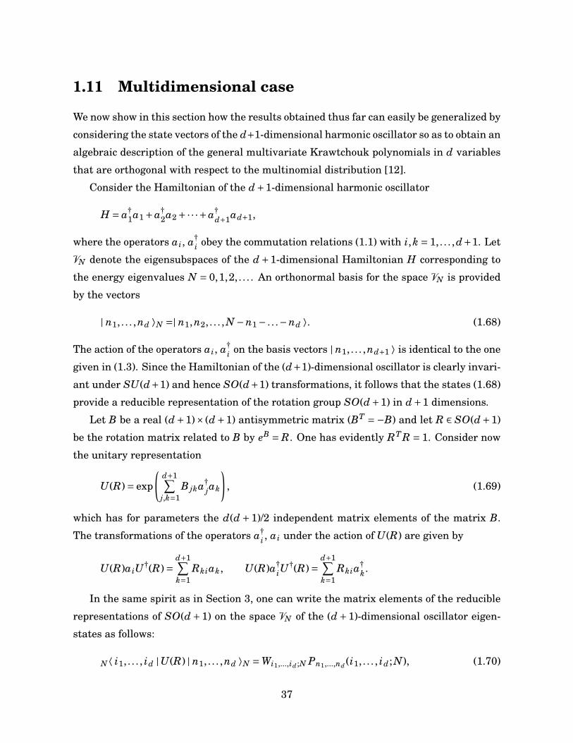
1.11 Multidimensional case
We now show in this section how the results obtained thus far can easily be generalized by
considering the state vectors of the d+1-dimensional harmonic oscillator so as to obtain an
algebraic description of the general multivariate Krawtchouk polynomials in d variables
that are orthogonal with respect to the multinomial distribution [12].
Consider the Hamiltonian of the d+1-dimensional harmonic oscillator
H = a†1a1 +a†
2a2 +·· ·+a†d+1ad+1,
where the operators ai, a†i obey the commutation relations (1.1) with i,k = 1, . . . ,d+1. Let
VN denote the eigensubspaces of the d+1-dimensional Hamiltonian H corresponding to
the energy eigenvalues N = 0,1,2, . . . . An orthonormal basis for the space VN is provided
by the vectors
| n1, . . . ,nd ⟩N =| n1,n2, . . . , N −n1 − . . .−nd ⟩. (1.68)
The action of the operators ai, a†i on the basis vectors | n1, . . . ,nd+1 ⟩ is identical to the one
given in (1.3). Since the Hamiltonian of the (d+1)-dimensional oscillator is clearly invari-
ant under SU(d+1) and hence SO(d+1) transformations, it follows that the states (1.68)
provide a reducible representation of the rotation group SO(d+1) in d+1 dimensions.
Let B be a real (d+1)× (d+1) antisymmetric matrix (BT =−B) and let R ∈ SO(d+1)
be the rotation matrix related to B by eB = R. One has evidently RTR = 1. Consider now
the unitary representation
U(R)= exp
(d+1∑j,k=1
B jka†jak
), (1.69)
which has for parameters the d(d +1)/2 independent matrix elements of the matrix B.
The transformations of the operators a†i , ai under the action of U(R) are given by
U(R)aiU†(R)=d+1∑k=1
Rkiak, U(R)a†iU
†(R)=d+1∑k=1
Rkia†k.
In the same spirit as in Section 3, one can write the matrix elements of the reducible
representations of SO(d +1) on the space VN of the (d +1)-dimensional oscillator eigen-
states as follows:
N⟨ i1, . . . , id |U(R) | n1, . . . ,nd ⟩N =Wi1,...,id ;N Pn1,...,nd (i1, . . . , id; N), (1.70)
37
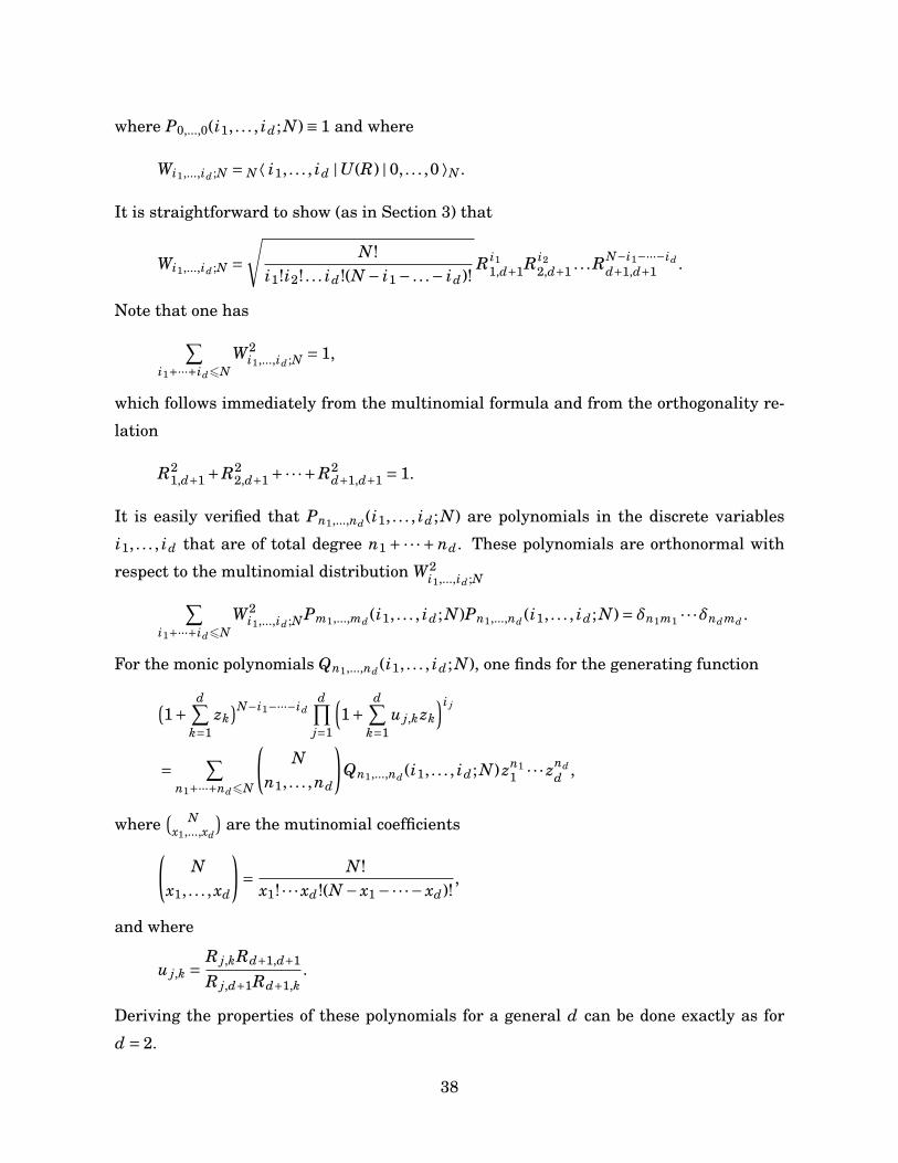
where P0,...,0(i1, . . . , id; N)≡ 1 and where
Wi1,...,id ;N = N⟨ i1, . . . , id |U(R) | 0, . . . ,0 ⟩N .
It is straightforward to show (as in Section 3) that
Wi1,...,id ;N =√
N!i1!i2! . . . id!(N − i1 − . . .− id)!
R i11,d+1R i2
2,d+1 . . .RN−i1−···−idd+1,d+1 .
Note that one has∑i1+···+id6N
W2i1,...,id ;N = 1,
which follows immediately from the multinomial formula and from the orthogonality re-
lation
R21,d+1 +R2
2,d+1 +·· ·+R2d+1,d+1 = 1.
It is easily verified that Pn1,...,nd (i1, . . . , id; N) are polynomials in the discrete variables
i1, . . . , id that are of total degree n1 + ·· · + nd. These polynomials are orthonormal with
respect to the multinomial distribution W2i1,...,id ;N∑
i1+···+id6NW2
i1,...,id ;NPm1,...,md (i1, . . . , id; N)Pn1,...,nd (i1, . . . , id; N)= δn1m1 · · ·δnd md .
For the monic polynomials Qn1,...,nd (i1, . . . , id; N), one finds for the generating function
(1+
d∑k=1
zk)N−i1−···−id
d∏j=1
(1+
d∑k=1
u j,kzk
)i j
= ∑n1+···+nd6N
(N
n1, . . . ,nd
)Qn1,...,nd (i1, . . . , id; N) zn1
1 · · · zndd ,
where( Nx1,...,xd
)are the mutinomial coefficients(
Nx1, . . . , xd
)= N!
x1! · · ·xd!(N − x1 −·· ·− xd)!,
and where
u j,k =R j,kRd+1,d+1
R j,d+1Rd+1,k.
Deriving the properties of these polynomials for a general d can be done exactly as for
d = 2.
38
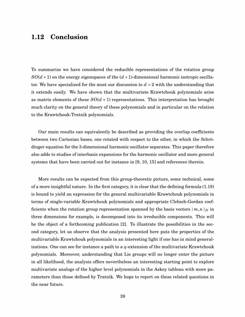
1.12 Conclusion
To summarize we have considered the reducible representations of the rotation group
SO(d+1) on the energy eigenspaces of the (d+1)-dimensional harmonic isotropic oscilla-
tor. We have specialized for the most our discussion to d = 2 with the understanding that
it extends easily. We have shown that the multivariate Krawtchouk polynomials arise
as matrix elements of these SO(d +1) representations. This interpretation has brought
much clarity on the general theory of these polynomials and in particular on the relation
to the Krawtchouk-Tratnik polynomials.
Our main results can equivalently be described as providing the overlap coefficients
between two Cartesian bases, one rotated with respect to the other, in which the Schrö-
dinger equation for the 3-dimensional harmonic oscillator separates. This paper therefore
also adds to studies of interbasis expansions for the harmonic oscillator and more general
systems that have been carried out for instance in [9, 10, 15] and references therein.
More results can be expected from this group-theoretic picture, some technical, some
of a more insightful nature. In the first category, it is clear that the defining formula (1.18)
is bound to yield an expression for the general multivariable Krawtchouk polynomials in
terms of single-variable Krawtchouk polynomials and appropriate Clebsch-Gordan coef-
ficients when the rotation group representation spanned by the basis vectors | m,n ⟩N in
three dimensions for example, is decomposed into its irreducible components. This will
be the object of a forthcoming publication [2]. To illustrate the possibilities in the sec-
ond category, let us observe that the analysis presented here puts the properties of the
multivariable Krawtchouk polynomials in an interesting light if one has in mind general-
izations. One can see for instance a path to a q-extension of the multivariate Krawtchouk
polynomials. Moreover, understanding that Lie groups will no longer enter the picture
in all likelihood, the analysis offers nevertheless an interesting starting point to explore
multivariate analogs of the higher level polynomials in the Askey tableau with more pa-
rameters than those defined by Tratnik. We hope to report on these related questions in
the near future.
39
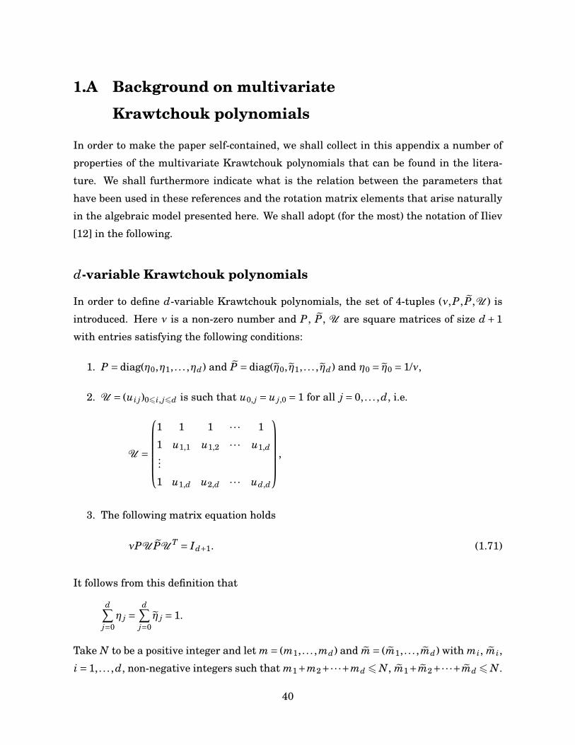
1.A Background on multivariate
Krawtchouk polynomials
In order to make the paper self-contained, we shall collect in this appendix a number of
properties of the multivariate Krawtchouk polynomials that can be found in the litera-
ture. We shall furthermore indicate what is the relation between the parameters that
have been used in these references and the rotation matrix elements that arise naturally
in the algebraic model presented here. We shall adopt (for the most) the notation of Iliev
[12] in the following.
d-variable Krawtchouk polynomials
In order to define d-variable Krawtchouk polynomials, the set of 4-tuples (ν,P, P,U ) is
introduced. Here ν is a non-zero number and P, P, U are square matrices of size d +1
with entries satisfying the following conditions:
1. P = diag(η0,η1, . . . ,ηd) and P = diag(η0, η1, . . . , ηd) and η0 = η0 = 1/ν,
2. U = (ui j)06i, j6d is such that u0, j = u j,0 = 1 for all j = 0, . . . ,d, i.e.
U =
1 1 1 · · · 1
1 u1,1 u1,2 · · · u1,d...
1 u1,d u2,d · · · ud,d
,
3. The following matrix equation holds
νPU PU T = Id+1. (1.71)
It follows from this definition that
d∑j=0
η j =d∑
j=0η j = 1.
Take N to be a positive integer and let m = (m1, . . . ,md) and m = (m1, . . . , md) with mi, mi,
i = 1, . . . ,d, non-negative integers such that m1+m2+·· ·+md 6 N, m1+m2+·· ·+md 6 N.
40
Following Griffiths [5], the polynomials Q(m, m) in the variables mi with degrees mi are
obtained from the generating function
d∏i=0
(1+
d∑j=1
ui, j z j
)mi = ∑m1+···md6N
N!m0!m1!m2! · · ·md!
Q(m, m)zm11 · · · zmd
m ,
where m0 = N −m1 −m2 −·· ·md and m0 = N − m1 − m2 −·· · md.
Identifying (n1, . . . ,nd) with (m1, . . . ,md) and (i1, . . . , id) with (m1, . . . , md), the poly-
nomials Pn1,...,nd (i1, . . . , id; N) introduced in (1.70) are the polynomials Q(m, m) up to a
normalization factor.
An explicit formula for Q(m, m) in terms of Gel’fand-Aomoto series has been given by
Mizukawa and Tanaka [24]:
Q(m, m)= ∑ai j
∏dj=1(−m j)∑d
i=1 ai j
∏di=1(−mi)∑d
j=1 ai, j
(−N)∑di, j ai, j
d∏i, j=1
ωai, ji, j
ai, j!, (1.72)
where ωi j = 1−ui j, ai j are non-negative integers such that∑d
i, j=1 ai, j 6 N.
Let
S21 = νP, S2
2 =Q, (1.73)
and set
V = S1U S2. (1.74)
It then follows that
VV T = S1U S2S2UTS1 = S1U QU TS1 = 1,
V is thus an orthogonal matrix and one has detV = ±1. By an appropriate choice of the
signs of the entries of the matrices S1 and S2, one can ensure that det(V ) = 1 so that
V corresponds to a proper rotation. Consequently, the rotation matrix R providing the
parameters for the general polynomials Qm,n(i,k; N) in our picture can be obtained from
V by rearranging the rows and columns.
41
Bivariate case
When d = 2, the above formulas have been specialized as follows. The matrix elements
ui j have been taken [13] to be parametrized by four numbers p1, p2, p3, p4 according to
u11 = 1− (p1 + p2)(p1 + p3)p1(p1 + p2 + p3 + p4)
= p1 p4 − p2 p3
p1(p1 + p2 + p3 + p4), (1.75a)
u12 = 1− (p1 + p2)(p2 + p4)p2(p1 + p2 + p3 + p4)
= p2 p3 − p1 p4
p2(p1 + p2 + p3 + p4), (1.75b)
u21 = 1− (p1 + p3)(p3 + p4)p3(p1 + p2 + p3 + p4)
= p2 p3 − p1 p4
p3(p1 + p2 + p3 + p4), (1.75c)
u22 = 1− (p2 + p4)(p3 + p4)p4(p1 + p2 + p3 + p4)
= p1 p4 − p2 p3
p4(p1 + p2 + p3 + p4), (1.75d)
with ηi and ηi given by
η1 = p1 p2(p1 + p2 + p3 + p4)(p1 + p2)(p1 + p3)(p2 + p4)
, η2 = p3 p4(p1 + p2 + p3 + p4)(p1 + p3)(p2 + p4)(p3 + p4)
, (1.76a)
η1 = p1 p3(p1 + p2 + p3 + p4)(p1 + p2)(p1 + p3)(p3 + p4)
, η2 = p2 p4(p1 + p2 + p3 + p4)(p1 + p2)(p2 + p4)(p3 + p4)
, (1.76b)
and where η0 = η0 = 1−η1−η2. The numbers p1, · · · , p4 are assumed to be arbitrary apart
for certain combinations that would lead to divisions by 0. It is checked that (1.71) is
satisfied with these definitions. It is also observed that these parameters are defined up
to an arbitrary common factor since the quadruplet (γp1,γp2,γp3,γp4) with an arbitrary
non-zero γ (γ 6= 0) leads to the same ui j as (p1, p2, p3, p4). This means that only three of
the four parameters pi are independent. This is related to the fact that 3-dimensional
rotations depend at most on 3 independent parameters like the Euler angles for instance.
The explicit formula (1.72) thus reduces to
Qm,n(m, n)= ∑i+ j+k+`6N
(−m)i+ j(−n)k+`(−m)i+k(−n) j+`i! j!k!`!(−N)i+ j+k+`
× (1−u11)i(1−u21) j(1−u12)k(1−u22)`. (1.77)
As for the generating function, it becomes
(1+u11z1 +u12z2)m1(1+u21z1 +u22z2)m2(1+ z1 + z2)m0
= ∑m1+m26N
N!m0!m1!m2!
Q(m, m)zm11 zm2
2 . (1.78)
From the identification (1.39) that brought the generating function (1.38) into the form
(1.78), we can express the parameters p1, . . . , p4 in terms of the rotation matrix elements.
42
One observes from (1.75) that
u11
u12=− p1
p2= R11R32
R31R12,
u21
u22=− p4
p3= R21R32
R31R22, (1.79a)
u12
u21= p3
p2= R12R23R31
R13R32R21,
u11
u22= p4
p1= R11R23R31
R13R31R21, (1.79b)
whence it is seen that one possible identification satisfying (1.79) is
p1 = R31
R11, p2 =−R32
R12, p3 =−R23R31
R13R21, p4 = R32R23
R13R22. (1.80)
One can use the affine latitude noted above to write down a more symmetric parametriza-
tion (by multiplying the above parameters by R31) where
p1 = R31R13
R11, p2 =−R32R13
R12, p3 =−R23R31
R21, p4 = R32R23
R22.
The expressions for η1, η2, η1 and η2 in terms of the rotation matrix elements Ri j can
also be determined. For instance, one obtains from (1.76) with the help of (1.75), (1.39)
and (1.79)
η1 = p2
p2 + p4
11+u11
= R213R22R31
(R13R22 −R12R23)(R13R31 −R11R33). (1.81)
Now given that detR = 1 and R−1 = RT , one has RT = adjR. This yields in particular,
R31 = R12R23 −R13R22, R22 = R11R33 −R13R31,
from where we find from (1.81) that η1 = R213. Similarly one arrives at
η2 = R223, η1 = R2
31, η2 = R232,
and η0 = η0 = 1− η1 − η2 = R233. This is in keeping with the fact that the polynomials
Q(m, m) are orthogonal with respect to the trinomial weight distribution
ω(m1, m2)= N!m1!m2!(N − m1 − m2)!
ηm11 η
m22 (1−η1 −η2)N−m1−m2 ,
that should be compared with formula (1.26).
In the multivariate case, the parameters ui j of the matrix U are related to those of
SO(d+1) rotations according to formulas (1.73) and (1.74). One may verify these relations
in the bivariate case with
S1 = diag(R33,R13,R23), S2 = diag(R33,R31,R32), ν= R33,
43
and the entries of U given by (1.39). A direct calculation shows that
V = 1ν
S1U S2 =
R33 R31 R32
R13 R11 R12
R23 R21 R22
,
which is the transpose of R after a cyclic permutation of the rows and columns.
Krawtchouk-Tratnik polynomials
Recall that the Krawtchouk-Tratnik polynomials K2(m,n; i,k;p1,p2; N) were seen to be a
special case of the Krawtchouk polynomials in two variables when R12 = 0 (or R21 = 0 as
a matter of fact). We note from (1.80) that the parametrization in terms of p1, p2, p3, p4
becomes singular in these instances. For completeness, let us record here the recurrence
relations that are satisfied by these polynomials. They are obtained directly from the
formulas given in Appendix A.3 of [3] and read (suppressing the parameters p1, p2 and
N):
i K2(m,n; i,k)=p1(m+n−N)[K2(m+1,n; i,k)−K2(m,n; i,k)
]+ (1−p1)m
[K2(m,n; i,k)−K2(m−1,n; i,k)
], (1.82a)
k K2(m,n; i,k)=[ p1p2
1−p1m+ (1−p1 −p2)
1−p1n+p2(N −m−n)
]K2(m,n; i,k),
− p2
1−p1mK2(m−1,n+1; i,k)−p1
(1−p1 −p2)1−p1
nK2(m+1,n−1; i,k)
+p2 mK2(m−1,n; i,k)+ p1p2
1−p1(N −n−m)K2(m+1,n; i,k) (1.82b)
− (1−p1 −p2)nK2(m,n−1; i,k)− p2
1−p1(N −n−m)K2(m,n+1; i,k).
To check that (1.43) reduces to (1.82b) when R12 = 0, given (1.61), one uses the relations
that correspond to RTR = 1 in this case, namely
R11R21 +R13R23 = R11R31 +R13R33 = 0, R211 +R2
13 = R222 +R2
32 = 1,
R22R21 +R32R31 = R22R23 +R32R33 = 0, R221 +R2
22 +R223 = R2
13 +R223 +R2
33 = 1,
to find for instance that
R232 =
1−p2
1−p1, R2
22 =1−p1 −p2
1−p2, R2
21 =p1p2
1−p1,
R211 = 1−p1, R2
33 = 1−p1 −p2, R231 = p1
(1−p1 −p2)1−p1
,
and to see that all the factors in (1.43) simplify then to those of (1.82b).
44
References
[1] I. Area, E. Godoy, and J. Rodal. On a class of bivariate second order linear partial differ-
ence equations and their monic orthogonal polynomial solutions. Journal of Mathematical
Analysis and Applications, 389:165–178, 2012.
[2] V.X. Genest, L. Vinet, and A. Zhedanov. Interbasis expansion for the isotropic 3D harmonic
oscillator and bivariate Krawtchouk polynomials. Journal of Physics A: Mathematical and
Theoretical, 47:025202, 2014.
[3] J.S. Geronimo and P. Iliev. Bispectrality of multivariable Racah-Wilson polynomials. Con-
structive Approximation, 31:417–457, 2010.
[4] Ya. I. Granovskii and A. Zhedanov. Orthogonal polynomials in the Lie algebras. Soviet
Physics Journal, 29:387–393, 1986.
[5] R.C. Griffiths. Orthogonal polynomials on the multinomial distribution. Australian Journal
of Statistics, 13:27–35, 1971.
[6] F.A. Grünbaum. The Rahman polynomials are bispectral. SIGMA, 3:65–75, 2007.
[7] F.A. Grünbaum and M. Rahman. On a family of 2-variable orthogonal Krawtchouk polyno-
mials. SIGMA, 6:90–101, 2010.
[8] F.A. Grünbaum and M. Rahman. A system of multivariable Krawtchouk polynomials and a
probabilistic application. SIGMA, 7:119–135, 2011.
[9] Ye. M. Hakobyan, G.S. Pogosyan, and A.N. Sissakian. On a Generalized D-Dimensional Os-
cillator: Interbasis Expansions. Physics of Atomic Nuclei, 61:1762–1767, 1998.
[10] Ye. M. Hakobyan, G.S. Pogosyan, A.N. Sissakian, and S.I. Vinitsky. Isotropic Oscillator in
the space of Constant Positive Curvature. Interbasis expansions. Physics of Atomic Nuclei,
64:671–685, 1999.
[11] M.R. Hoare and M. Rahman. A probabilistic origin for a new class of bivariate polynomials.
SIGMA, 4:89–106, 2008.
[12] P. Iliev. A Lie-theoretic interpretation of multivariate hypergeometric polynomials. Compo-
sitio Mathematica, 148:991–1002, 2012.
[13] P. Iliev and P. Terwilliger. The Rahman polynomials and the Lie algebras sl3(C). Transactions
of the American Mathematical Society, 364:4225–4238, 2012.
45
[14] P. Iliev and Y. Xu. Discrete orthogonal polynomials and difference equations in several vari-
ables. Advances in Mathematics, 212:1–36, 2007.
[15] E.G. Kalnins, W. Miller, and S. Post. Two-Variable Wilson Polynomials and the Generic Su-
perintegrable System on the 3-Sphere. SIGMA, 7:51–76, 2011.
[16] S. Karlin and J. McGregor. Linear growth models with many types and multidimensional
Hahn polynomials. In R.A. Askey, editor, Theory and applications of special functions, pages
261–288. Academic Press, 1975.
[17] R. Koekoek, P.A. Lesky, and R.F. Swarttouw. Hypergeometric orthogonal polynomials and
their q-analogues. Springer, 1st edition, 2010.
[18] T. Koornwinder. Krawtchouk polynomials, a unification of two different group theoretic in-
terpretations. SIAM Journal of Mathematical Analysis, 13:1011–1023, 1982.
[19] M. Krawtchouk. Sur une généralisation des polynômes d’Hermite. Comptes Rendus Mathé-
matiques, 189:620–622, 1929.
[20] H. Miki, S. Tsujimoto, L. Vinet, and A. Zhedanov. Quantum-state transfer in a two-
dimensional regular spin lattice of triangular shape. Physical Review A, 85:062306, 2012.
[21] M. Miki, S. Post, L. Vinet, and A. Zhedanov. A superintegrable finite oscillator in two dimen-
sions with SU(2) symmetry. Journal of Physics A: Mathematical and Theoretical, 46:125207,
2013.
[22] P.R. Milch. A multi-dimensional linear growth birth and death process. Annals of Mathemat-
ical Statistics, 39:727–754, 1968.
[23] H. Mizukawa. Orthogonality relations for multivariate Krawtchouk polynomials. SIGMA,
7:117, 2011.
[24] H. Mizukawa and H. Tanaka. (n+1,m+1)-hypergeometric functions associated to character
algebras. Proceedings of the American Mathematical Society, 132:2613–2618, 2004.
[25] A. F. Nikiforov, S. K. Suslov, and V. B. Uvarov. Classical orthogonal polynomials of a discrete
variable. Springer Series in Computational Physics. Springer, 1991.
[26] A.V. Rosenblyum. Spectral analysis of generators of representations of the group U(3). The-
oretical and Mathematical Physics, 73:1352–1356, 1987.
[27] M.V. Tratnik. Some multivariable orthogonal polynomials of the Askey tableau-discrete fam-
ilies. Journal of Mathematical Physics, 32:2337–2342, 1991.
46
[28] Y. Xu. On discrete orthogonal polynomials of several variables. Advances in Applied Mathe-
matics, 33:615–632, 2004.
[29] A. Zhedanov. 9 j-symbols of the oscillator algebra and Krawtchouk polynomials in two vari-
ables. Journal of Physics A: Mathematical and General, 30:8337–8357, 1997.
47

48
Chapitre 2
The multivariate Meixnerpolynomials as matrix elements ofSO(d,1) representations on oscillatorstates
V. X. Genest, H. Miki, L. Vinet et A. Zhedanov (2014). The multivariate Meixner polynomials as
matrix elements of SO(d,1) representations on oscillator states. Journal of Physics A: Mathemat-
ical and Theoretical 47 045207
Abstract. The multivariate Meixner polynomials are shown to arise as matrix elements of unitary
representations of the SO(d,1) group on oscillator states. These polynomials depend on d discrete
variables and are orthogonal with respect to the negative multinomial distribution. The emphasis
is put on the bivariate case for which the SO(2,1) connection is used to derive the main prop-
erties of the polynomials: orthogonality relation, raising/lowering relations, generating function,
recurrence relations and difference equations as well as explicit expressions in terms of standard
(univariate) Krawtchouk and Meixner polynomials. It is explained how these results generalize
directly to d variables.
2.1 Introduction
The objective of this paper is to provide a group theoretical interpretation of the multivariate
Meixner polynomials and to show how their properties naturally follow from this picture. The
Meixner polynomials in d variables will be shown to arise as matrix elements of the reducible
49
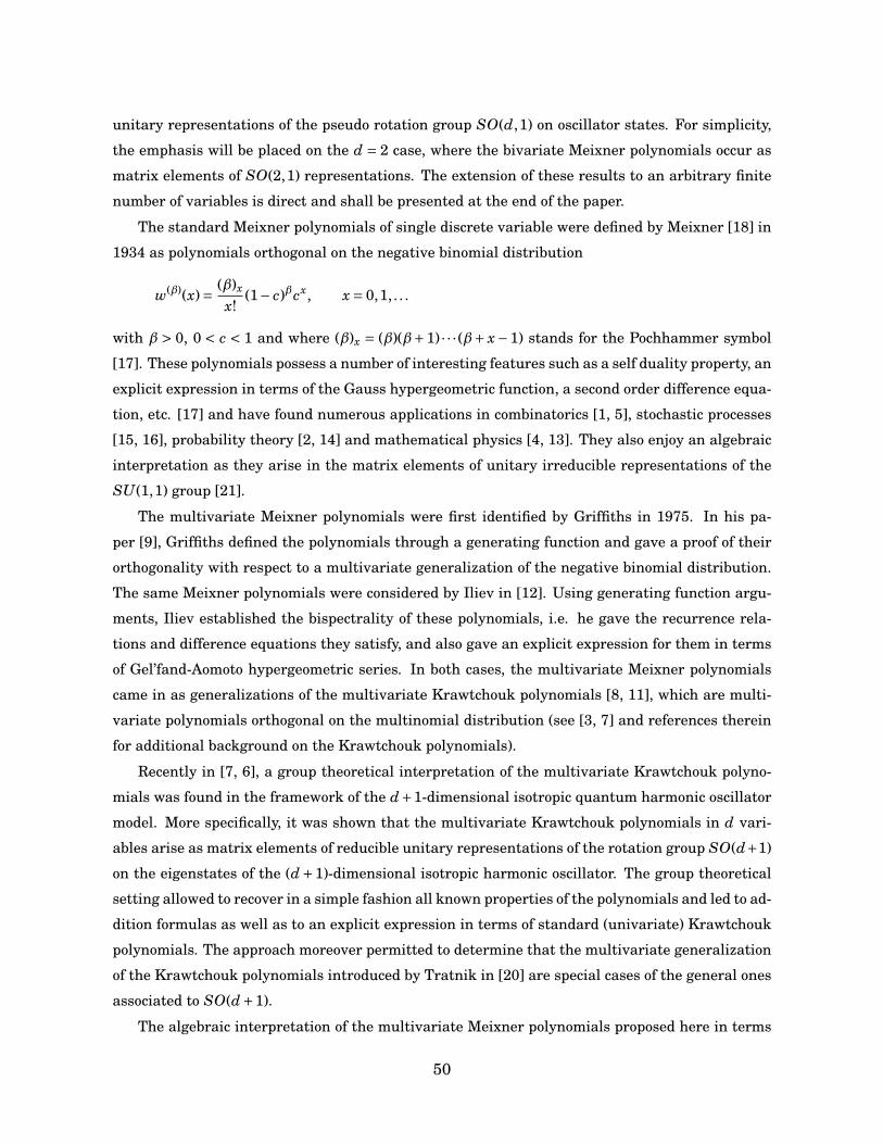
unitary representations of the pseudo rotation group SO(d,1) on oscillator states. For simplicity,
the emphasis will be placed on the d = 2 case, where the bivariate Meixner polynomials occur as
matrix elements of SO(2,1) representations. The extension of these results to an arbitrary finite
number of variables is direct and shall be presented at the end of the paper.
The standard Meixner polynomials of single discrete variable were defined by Meixner [18] in
1934 as polynomials orthogonal on the negative binomial distribution
w(β)(x)= (β)x
x!(1− c)βcx, x = 0,1, . . .
with β > 0, 0 < c < 1 and where (β)x = (β)(β+1) · · · (β+ x−1) stands for the Pochhammer symbol
[17]. These polynomials possess a number of interesting features such as a self duality property, an
explicit expression in terms of the Gauss hypergeometric function, a second order difference equa-
tion, etc. [17] and have found numerous applications in combinatorics [1, 5], stochastic processes
[15, 16], probability theory [2, 14] and mathematical physics [4, 13]. They also enjoy an algebraic
interpretation as they arise in the matrix elements of unitary irreducible representations of the
SU(1,1) group [21].
The multivariate Meixner polynomials were first identified by Griffiths in 1975. In his pa-
per [9], Griffiths defined the polynomials through a generating function and gave a proof of their
orthogonality with respect to a multivariate generalization of the negative binomial distribution.
The same Meixner polynomials were considered by Iliev in [12]. Using generating function argu-
ments, Iliev established the bispectrality of these polynomials, i.e. he gave the recurrence rela-
tions and difference equations they satisfy, and also gave an explicit expression for them in terms
of Gel’fand-Aomoto hypergeometric series. In both cases, the multivariate Meixner polynomials
came in as generalizations of the multivariate Krawtchouk polynomials [8, 11], which are multi-
variate polynomials orthogonal on the multinomial distribution (see [3, 7] and references therein
for additional background on the Krawtchouk polynomials).
Recently in [7, 6], a group theoretical interpretation of the multivariate Krawtchouk polyno-
mials was found in the framework of the d+1-dimensional isotropic quantum harmonic oscillator
model. More specifically, it was shown that the multivariate Krawtchouk polynomials in d vari-
ables arise as matrix elements of reducible unitary representations of the rotation group SO(d+1)
on the eigenstates of the (d+1)-dimensional isotropic harmonic oscillator. The group theoretical
setting allowed to recover in a simple fashion all known properties of the polynomials and led to ad-
dition formulas as well as to an explicit expression in terms of standard (univariate) Krawtchouk
polynomials. The approach moreover permitted to determine that the multivariate generalization
of the Krawtchouk polynomials introduced by Tratnik in [20] are special cases of the general ones
associated to SO(d+1).
The algebraic interpretation of the multivariate Meixner polynomials proposed here in terms
50
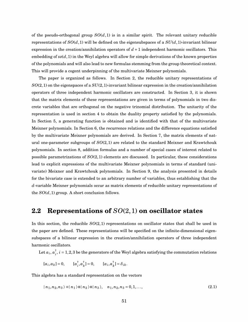
of the pseudo-orthogonal group SO(d,1) is in a similar spirit. The relevant unitary reducible
representations of SO(d,1) will be defined on the eigensubspaces of a SU(d,1)-invariant bilinear
expression in the creation/annihilation operators of d+1 independent harmonic oscillators. This
embedding of so(d,1) in the Weyl algebra will allow for simple derivations of the known properties
of the polynomials and will also lead to new formulas stemming from the group theoretical context.
This will provide a cogent underpinning of the multivariate Meixner polynomials.
The paper is organized as follows. In Section 2, the reducible unitary representations of
SO(2,1) on the eigenspaces of a SU(2,1)-invariant bilinear expression in the creation/annihilation
operators of three independent harmonic oscillators are constructed. In Section 3, it is shown
that the matrix elements of these representations are given in terms of polynomials in two dis-
crete variables that are orthogonal on the negative trinomial distribution. The unitarity of the
representation is used in section 4 to obtain the duality property satisfied by the polynomials.
In Section 5, a generating function is obtained and is identified with that of the multivariate
Meixner polynomials. In Section 6, the recurrence relations and the difference equations satisfied
by the multivariate Meixner polynomials are derived. In Section 7, the matrix elements of nat-
ural one-parameter subgroups of SO(2,1) are related to the standard Meixner and Krawtchouk
polynomials. In section 8, addition formulas and a number of special cases of interest related to
possible parametrizations of SO(2,1) elements are discussed. In particular, these considerations
lead to explicit expressions of the multivariate Meixner polynomials in terms of standard (uni-
variate) Meixner and Krawtchouk polynomials. In Section 9, the analysis presented in details
for the bivariate case is extended to an arbitrary number of variables, thus establishing that the
d-variable Meixner polynomials occur as matrix elements of reducible unitary representations of
the SO(d,1) group. A short conclusion follows.
2.2 Representations of SO(2,1) on oscillator states
In this section, the reducible SO(2,1) representations on oscillator states that shall be used in
the paper are defined. These representations will be specified on the infinite-dimensional eigen-
subspaces of a bilinear expression in the creation/annihilation operators of three independent
harmonic oscillators.
Let ai, a†i , i = 1,2,3 be the generators of the Weyl algebra satisfying the commutation relations
[ai,ak]= 0, [a†i ,a
†k]= 0, [ai,a
†k]= δik.
This algebra has a standard representation on the vectors
| n1,n2,n3 ⟩ ≡| n1 ⟩⊗| n2 ⟩⊗| n3 ⟩, n1,n2,n3 = 0,1, . . . , (2.1)
51
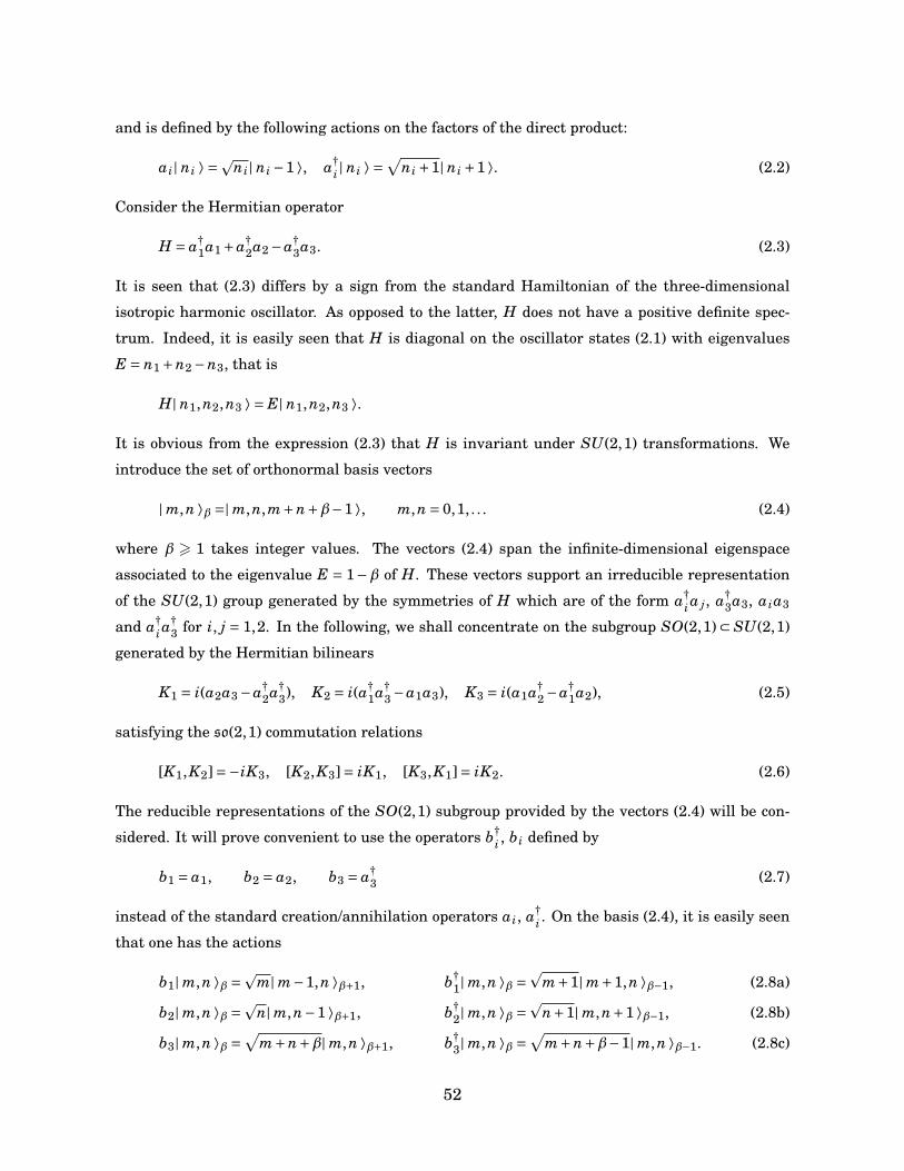
and is defined by the following actions on the factors of the direct product:
ai| ni ⟩ =pni| ni −1 ⟩, a†
i | ni ⟩ =√
ni +1| ni +1 ⟩. (2.2)
Consider the Hermitian operator
H = a†1a1 +a†
2a2 −a†3a3. (2.3)
It is seen that (2.3) differs by a sign from the standard Hamiltonian of the three-dimensional
isotropic harmonic oscillator. As opposed to the latter, H does not have a positive definite spec-
trum. Indeed, it is easily seen that H is diagonal on the oscillator states (2.1) with eigenvalues
E = n1 +n2 −n3, that is
H| n1,n2,n3 ⟩ = E| n1,n2,n3 ⟩.
It is obvious from the expression (2.3) that H is invariant under SU(2,1) transformations. We
introduce the set of orthonormal basis vectors
| m,n ⟩β =| m,n,m+n+β−1 ⟩, m,n = 0,1, . . . (2.4)
where β > 1 takes integer values. The vectors (2.4) span the infinite-dimensional eigenspace
associated to the eigenvalue E = 1−β of H. These vectors support an irreducible representation
of the SU(2,1) group generated by the symmetries of H which are of the form a†i a j, a†
3a3, aia3
and a†i a
†3 for i, j = 1,2. In the following, we shall concentrate on the subgroup SO(2,1) ⊂ SU(2,1)
generated by the Hermitian bilinears
K1 = i(a2a3 −a†2a†
3), K2 = i(a†1a†
3 −a1a3), K3 = i(a1a†2 −a†
1a2), (2.5)
satisfying the so(2,1) commutation relations
[K1,K2]=−iK3, [K2,K3]= iK1, [K3,K1]= iK2. (2.6)
The reducible representations of the SO(2,1) subgroup provided by the vectors (2.4) will be con-
sidered. It will prove convenient to use the operators b†i , bi defined by
b1 = a1, b2 = a2, b3 = a†3 (2.7)
instead of the standard creation/annihilation operators ai, a†i . On the basis (2.4), it is easily seen
that one has the actions
b1| m,n ⟩β =p
m| m−1,n ⟩β+1, b†1| m,n ⟩β =
pm+1| m+1,n ⟩β−1, (2.8a)
b2| m,n ⟩β =p
n| m,n−1 ⟩β+1, b†2| m,n ⟩β =
pn+1| m,n+1 ⟩β−1, (2.8b)
b3| m,n ⟩β =√
m+n+β| m,n ⟩β+1, b†3| m,n ⟩β =
√m+n+β−1| m,n ⟩β−1. (2.8c)
52
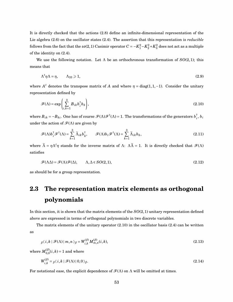
It is directly checked that the actions (2.8) define an infinite-dimensional representation of the
Lie algebra (2.6) on the oscillator states (2.4). The assertion that this representation is reducible
follows from the fact that the so(2,1) Casimir operator C =−K21−K2
2+K23 does not act as a multiple
of the identity on (2.4).
We use the following notation. Let Λ be an orthochronous transformation of SO(2,1); this
means that
ΛtηΛ= η, Λ33 > 1, (2.9)
where At denotes the transpose matrix of A and where η = diag(1,1,−1). Consider the unitary
representation defined by
F (Λ)= exp
(3∑
i,k=1Bikb†
i bk
), (2.10)
where Bik =−Bki. One has of course F (Λ)F †(Λ)= 1. The transformations of the generators b†i , bi
under the action of F (Λ) are given by
F (Λ)b†iF
†(Λ)=3∑
k=1Λikb†
k, F (Λ)biF†(Λ)=
3∑k=1
Λikbk, (2.11)
where Λ = ηΛtη stands for the inverse matrix of Λ: ΛΛ = 1. It is directly checked that F (Λ)
satisfies
F (Λ∆)=F (Λ)F (∆), Λ,∆ ∈ SO(2,1), (2.12)
as should be for a group representation.
2.3 The representation matrix elements as orthogonal
polynomials
In this section, it is shown that the matrix elements of the SO(2,1) unitary representation defined
above are expressed in terms of orthogonal polynomials in two discrete variables.
The matrix elements of the unitary operator (2.10) in the oscillator basis (2.4) can be written
as
β⟨ i,k |F (Λ) | m,n ⟩β =W (β)i,k M(β)
m,n(i,k), (2.13)
where M(β)0,0(i,k)= 1 and where
W (β)i,k = β⟨ i,k |F (Λ) | 0,0 ⟩β. (2.14)
For notational ease, the explicit dependence of F (Λ) on Λ will be omitted at times.
53
2.3.1 Calculation of W (β)i,k
To derive the explicit expression of the amplitude W (β)i,k , one first observes that
β+1⟨ i,k |F b j | 0,0 ⟩β = 0,
for j = 1,2. Since β+1⟨ i,k | F b j | 0,0 ⟩β = β⟨ i,k | F b jF†F | 0,0 ⟩β, one obtains, using (2.11), the
following system of difference equations for Wβ
i,k:
Λ11p
i+1W (β)i+1,k + Λ12
pk+1W (β)
i,k+1 + Λ13√
i+k+βW (β)i,k = 0, (2.15a)
Λ21p
i+1W (β)i+1,k + Λ22
pk+1W (β)
i,k+1 + Λ23√
i+k+βW (β)i,k = 0. (2.15b)
Using the fact that ΛηΛtη= 1, it is readily seen that the solution to the system (2.15) is of the form
W (β)i,k =
√(β)i+k
i!k!
(− Λ31
Λ33
)i (− Λ32
Λ33
)k
W (β)0,0 ,
where W (β)0,0 = β⟨ 0,0 | F | 0,0 ⟩β. The constant W (β)
0,0 can be obtained from the normalization condi-
tion
1= β⟨ 0,0 |F †F | 0,0 ⟩β =∑
i,k>0β⟨ i,k |F | 0,0 ⟩ββ⟨ 0,0 |F † | i,k ⟩β =
∑i,k>0
|W (β)i,k |2.
One can then use the formula
(1− z1 − z2)−β =∑i,k
(β)i+k
i!k!zi
1zk2 ,
which holds provided that |z1|+ |z2| < 1. It is directly seen from (2.9) that this condition is identi-
cally satisfied and hence one finds that W (β)0,0 = [Λ33]−β. In terms of the matrix elements of Λ, the
complete expression for the amplitude W (β)i,k is thus found to be
W (β)i,k =
√(β)i+k
i!k!(Λ33
)−β−i−kΛi
13Λk23. (2.16)
2.3.2 Raising relations
To show that the M(β)m,n(i,k) appearing in the matrix elements (2.13) are polynomials of total degree
m+ n in the two variables i, k, one can examine their raising relations, which are obtained as
follows. One has on the one hand
β⟨ i,k |F b†1 | m,n ⟩β+1 =
pm+1W (β)
i,k M(β)m+1,n(i,k),
β⟨ i,k |F b†2 | m,n ⟩β+1 =
pn+1W (β)
i,k M(β)m,n+1(i,k).
54
On the other hand, using (2.11), one has
β⟨ i,k |F b†1 | m,n ⟩β+1 = β⟨ i,k |F b†
1 F †F | m,n ⟩β+1 =3∑
j=1Λ1 j β⟨ i,k | b†
j F | m,n ⟩β+1,
β⟨ i,k |F b†2 | m,n ⟩β+1 = β⟨ i,k |F b†
2 F †F | m,n ⟩β+1 =3∑
j=1Λ2 j β⟨ i,k | b†
j F | m,n ⟩β+1.
Upon combining the above relations, one obtains the raising relations√β(m+1) M(β)
m+1,n(i,k)=Λ11
Λ13i M(β+1)
m,n (i−1,k)+ Λ21
Λ23k M(β+1)
m,n (i,k−1)
− Λ31
Λ33(i+k+β) M(β+1)
m,n (i,k),(2.17a)
√β(n+1) M(β)
m,n+1(i,k)=Λ12
Λ13i M(β+1)
m,n (i−1,k)+ Λ22
Λ23k M(β+1)
m,n (i,k−1)
− Λ32
Λ33(i+k+β) M(β+1)
m,n (i,k).(2.17b)
By definition, one has M(β)−1,n(i,k) = M(β)
m,−1(i,k) = 0 and M(β)0,0(i,k) = 1. Therefore, the formulas
(2.17) can be used to construct M(β)m,n(i,k) from M(β)
0,0(i,k) iteratively. Furthermore, it is observed
that M(β)m,n(i,k) are polynomials of total degree m+n in the discrete variables i and k.
2.3.3 Orthogonality Relation
It follows from the unitarity of the representation (2.10) and the orthonormality of the oscilla-
tor states that the polynomials M(β)m,n(i,k) are orthogonal with respect to the negative trinomial
distribution. Indeed, one has
β⟨ m′,n′ |F †F | m,n ⟩β =∑
i,k>0β⟨ i,k |F | m,n ⟩ββ⟨ m′,n′ |F † | i,k ⟩β = δmm′δnn′ .
Upon using (2.13), one finds that the polynomials satisfy the orthogonality relation∑i,k>0
w(β)i,k M(β)
m,n(i,k) M(β)m′,n′(i,k)= δmm′δnn′ , (2.18)
where w(β)i,k is the negative trinomial distribution
w(β)i,k = (β)i+k
i!k!(1− c1 − c2)βci
1ck2, (2.19)
with
c1 =Λ2
13
Λ233
, c2 =Λ2
23
Λ233
.
Recall that in view of (2.9), the condition |c1| + |c2| < 1 is identically satisfied for orthochronous
elements of SO(2,1).
55
2.3.4 Lowering Relations
Lowering relations for the polynomials M(β)m,n(i,k) can also be obtained. To this end, one first
considers the matrix elements β⟨ i,k |F b j | m,n ⟩β−1 with j = 1,2. One has on the one hand
β⟨ i,k |F b1 | m,n ⟩β−1 =p
mW (β)i,k M(β)
m−1,n(i,k),
β⟨ i,k |F b2 | m,n ⟩β−1 =p
nW (β)i,k M(β)
m,n−1(i,k),
and on the other hand
β⟨ i,k |F b j | m,n ⟩β−1 = β⟨ i,k |F b j F†F | m,n ⟩β−1 =
3∑`=1
Λ j` β⟨ i,k | b`F | m,n ⟩β−1.
Upon comparing the two expressions, a simple calculation yields√m
β−1M(β)
m−1,n(i,k)=Λ11Λ13[M(β−1)
m,n (i+1,k)−M(β−1)m,n (i,k)
]+Λ21Λ23
[M(β−1)
m,n (i,k+1)−M(β−1)m,n (i,k)
],
(2.20a)
√n
β−1M(β)
m,n−1(i,k)=Λ12Λ13[M(β−1)
m,n (i+1,k)−M(β−1)m,n (i,k)
]+Λ22Λ23
[M(β−1)
m,n (i,k+1)−M(β−1)m,n (i,k)
].
(2.20b)
2.4 Duality
In this section, a duality relation under the exchange of the degrees m, n and the variables i,
k is derived for the multivariate polynomials M(β)m,n(i,k). For the monic polynomials R(β)
m,n(i,k),
which are obtained from the M(β)m,n(i,k) by a normalization, this duality property is seen to take a
particularly simple form.
The duality relation for the polynomials M(β)m,n(i,k) is found by considering the matrix elements
β⟨ i,k |F †(Λ) | m,n ⟩β from two different points of view. First, one writes
β⟨ i,k |F †(Λ) | m,n ⟩β = W (β)i,k M(β)
m,n(i,k), (2.21)
where W (β)i,k = β⟨ i,k |F †(Λ) | 0,0 ⟩β and M(β)
0,0(i,k)= 1. On account of the fact that F †(Λ)=F (Λ−1)=F (ηΛtη), it follows that
W (β)i,k =
√(β)i+k
i!k!(Λ33
)−β−i−k(−Λ31)i(−Λ32)k,
56
and that M(β)m,n(i,k) are the polynomials corresponding to the matrix Λ= ηΛtη. Second, one writes
β⟨ i,k |F †(Λ) | m,n ⟩β = β⟨ m,n |F (Λ) | i,k ⟩β= β⟨ m,n |F (Λ) | i,k ⟩β =W (β)
m,n M(β)i,k(m,n),
(2.22)
where x stands for complex conjugation and where the reality of the matrix elements has been
used. Upon comparing (2.21) and (2.22), one obtains the duality relation
M(β)i,k(m,n)= (−1)i+k
√(β)i+k
i!k!m!n!
(β)m+n
Λm+n33 Λi
31Λk32
Λi+k33 Λm
13Λn23
M(β)m,n(i,k). (2.23)
It is opportune here to introduce the monic polynomials R(β)m,n(i,k) defined by
M(β)m,n(i,k)= (−1)m+n
√(β)m+n
m!n!Λm
31Λn32
Λm+n33
R(β)m,n(i,k).
In terms of these polynomials, the duality relation (2.23) has the attractive expression
R(β)i,k(m,n)= R(β)
m,n(i,k), (2.24)
where the parameters appearing in the polynomials R(β)m,n(i,k) are those of the inverse matrix
Λ= ηΛtη.
2.5 Generating function and
hypergeometric expression
In this section, generating functions for the multivariate polynomials M(β)m,n(i,k) and R(β)
m,n(i,k) are
obtained using the group product. The generating function derived for the polynomials R(β)m,n(i,k) is
shown to coincide with the one defining the multivariate Meixner polynomials, which establishes
that the polynomials R(β)m,n(i,k) are precisely those defined in [9] and [12]. Using the results of [12],
an explicit expression of the polynomials R(β)m,n(i,k) in terms of Gel’fand-Aomoto hypergeometric
series is given.
2.5.1 Generating function
Let ∆ ∈ SO(2,1) be an arbitrary group element and consider the following generating function:
G(∆)= ∑m,n>0
√(β)m+n
m!n!∆−β−m−n33 ∆m
13∆n23 W (β)
i,k M(β)m,n(i,k). (2.25)
57
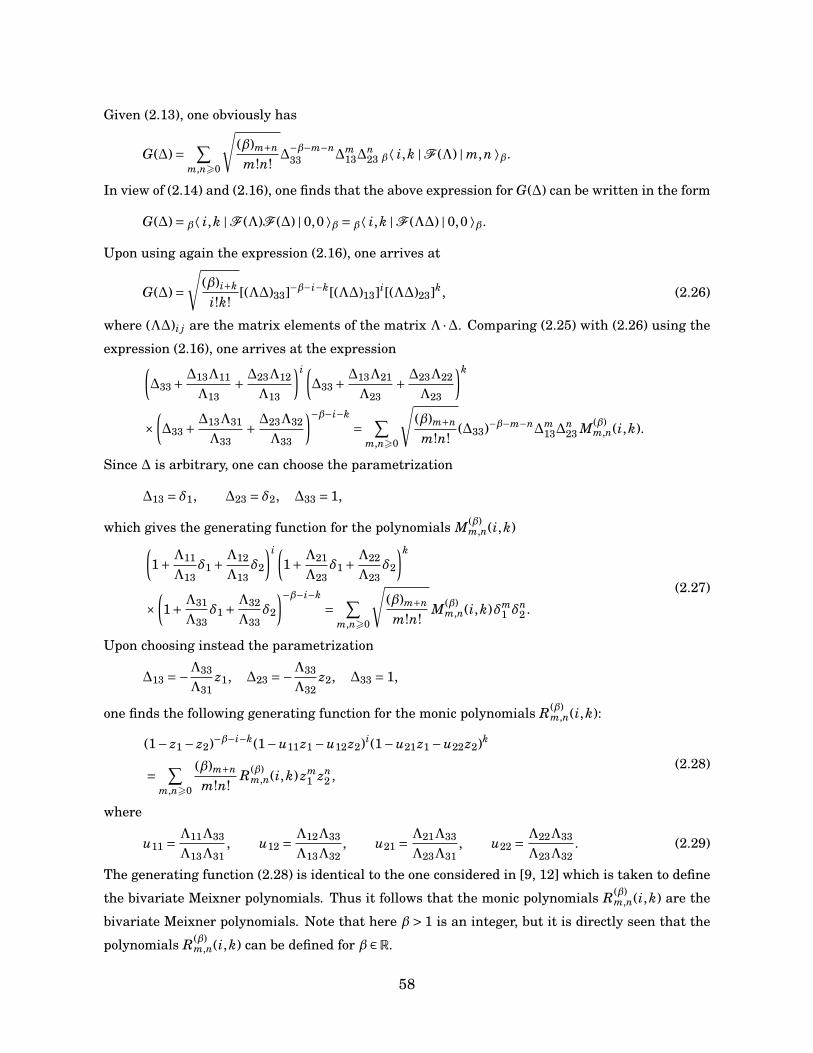
Given (2.13), one obviously has
G(∆)= ∑m,n>0
√(β)m+n
m!n!∆−β−m−n33 ∆m
13∆n23 β⟨ i,k |F (Λ) | m,n ⟩β.
In view of (2.14) and (2.16), one finds that the above expression for G(∆) can be written in the form
G(∆)= β⟨ i,k |F (Λ)F (∆) | 0,0 ⟩β = β⟨ i,k |F (Λ∆) | 0,0 ⟩β.
Upon using again the expression (2.16), one arrives at
G(∆)=√
(β)i+k
i!k![(Λ∆)33]−β−i−k[(Λ∆)13]i[(Λ∆)23]k, (2.26)
where (Λ∆)i j are the matrix elements of the matrix Λ ·∆. Comparing (2.25) with (2.26) using the
expression (2.16), one arrives at the expression(∆33 + ∆13Λ11
Λ13+ ∆23Λ12
Λ13
)i (∆33 + ∆13Λ21
Λ23+ ∆23Λ22
Λ23
)k
×(∆33 + ∆13Λ31
Λ33+ ∆23Λ32
Λ33
)−β−i−k= ∑
m,n>0
√(β)m+n
m!n!(∆33)−β−m−n∆m
13∆n23 M(β)
m,n(i,k).
Since ∆ is arbitrary, one can choose the parametrization
∆13 = δ1, ∆23 = δ2, ∆33 = 1,
which gives the generating function for the polynomials M(β)m,n(i,k)(
1+ Λ11
Λ13δ1 + Λ12
Λ13δ2
)i (1+ Λ21
Λ23δ1 + Λ22
Λ23δ2
)k
×(1+ Λ31
Λ33δ1 + Λ32
Λ33δ2
)−β−i−k= ∑
m,n>0
√(β)m+n
m!n!M(β)
m,n(i,k)δm1 δ
n2 .
(2.27)
Upon choosing instead the parametrization
∆13 =−Λ33
Λ31z1, ∆23 =−Λ33
Λ32z2, ∆33 = 1,
one finds the following generating function for the monic polynomials R(β)m,n(i,k):
(1− z1 − z2)−β−i−k(1−u11z1 −u12z2)i(1−u21z1 −u22z2)k
= ∑m,n>0
(β)m+n
m!n!R(β)
m,n(i,k) zm1 zn
2 ,(2.28)
where
u11 = Λ11Λ33
Λ13Λ31, u12 = Λ12Λ33
Λ13Λ32, u21 = Λ21Λ33
Λ23Λ31, u22 = Λ22Λ33
Λ23Λ32. (2.29)
The generating function (2.28) is identical to the one considered in [9, 12] which is taken to define
the bivariate Meixner polynomials. Thus it follows that the monic polynomials R(β)m,n(i,k) are the
bivariate Meixner polynomials. Note that here β> 1 is an integer, but it is directly seen that the
polynomials R(β)m,n(i,k) can be defined for β ∈R.
58
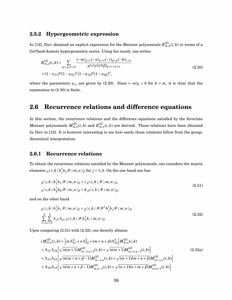
2.5.2 Hypergeometric expression
In [12], Iliev obtained an explicit expression for the Meixner polynomials R(β)m,n(i,k) in terms of a
Gel’fand-Aomoto hypergeometric series. Using his result, one writes
R(β)m,n(i,k)= ∑
µ,ν,ρ,σ>0
(−m)µ+ν(−n)ρ+σ(−i)µ+ρ(−k)ν+σµ!ν!ρ!σ!(β)µ+ν+ρ+σ
× (1−u11)µ(1−u21)ν(1−u12)ρ(1−u22)σ,
(2.30)
where the parameters ui j are given by (2.29). Since (−m)k = 0 for k > m, it is clear that the
summation in (2.30) is finite.
2.6 Recurrence relations and difference equations
In this section, the recurrence relations and the difference equations satisfied by the bivariate
Meixner polynomials M(β)m,n(i,k) and R(β)
m,n(i,k) are derived. These relations have been obtained
by Iliev in [12]. It is however interesting to see how easily these relations follow from the group-
theoretical interpretation.
2.6.1 Recurrence relations
To obtain the recurrence relations satisfied by the Meixner polynomials, one considers the matrix
elements β⟨ i,k | b†jb jF | m,n ⟩β for j = 1,2. On the one hand one has
β⟨ i,k | b†1b1 F | m,n ⟩β = i β⟨ i,k |F | m,n ⟩β,
β⟨ i,k | b†2b2 F | m,n ⟩β = k β⟨ i,k |F | m,n ⟩β,
(2.31)
and on the other hand
β⟨ i,k | b†jb j F | m,n ⟩β = β⟨ i,k |FF †b†
jb jF | m,n ⟩β3∑
`=1
3∑r=1
Λ j`Λ jr β⟨ i,k |F b†`br | m,n ⟩β.
(2.32)
Upon comparing (2.31) with (2.32), one directly obtains
i M(β)m,n(i,k)=
[mΛ2
11 +nΛ212 + (m+n+β)Λ2
13
]M(β)
m,n(i,k)
+Λ11Λ12
[√m(n+1)M(β)
m−1,n+1(i,k)+√
n(m+1)M(β)m+1,n−1(i,k)
](2.33a)
+Λ11Λ13
[√m(m+n+β−1)M(β)
m−1,n(i,k)+√
(m+1)(m+n+β)M(β)m+1,n(i,k)
]+Λ12Λ13
[√n(m+n+β−1)M(β)
m,n−1(i,k)+√
(n+1)(n+m+β)M(β)m,n+1(i,k)
]
59
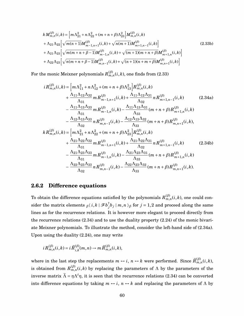
k M(β)m,n(i,k)=
[mΛ2
21 +nΛ222 + (m+n+β)Λ2
23
]M(β)
m,n(i,k)
+Λ21Λ22
[√m(n+1)M(β)
m−1,n+1(i,k)+√
n(m+1)M(β)m+1,n−1(i,k)
](2.33b)
+Λ21Λ23
[√m(m+n+β−1)M(β)
m−1,n(i,k)+√
(m+1)(m+n+β)M(β)m+1,n(i,k)
]+Λ22Λ23
[√n(m+n+β−1)M(β)
m,n−1(i,k)+√
(n+1)(n+m+β)M(β)m,n+1(i,k)
]For the monic Meixner polynomials R(β)
m,n(i,k), one finds from (2.33)
i R(β)m,n(i,k)=
[mΛ2
11 +nΛ212 + (m+n+β)Λ2
13
]R(β)
m,n(i,k)
+ Λ11Λ12Λ32
Λ31mR(β)
m−1,n+1(i,k)+ Λ11Λ12Λ31
Λ32nR(β)
m+1,n−1(i,k) (2.34a)
− Λ11Λ13Λ33
Λ31mR(β)
m−1,n(i,k)− Λ11Λ13Λ31
Λ33(m+n+β)R(β)
m+1,n(i,k)
− Λ12Λ13Λ33
Λ32nR(β)
m,n−1(i,k)− Λ12Λ13Λ32
Λ33(m+n+β)R(β)
m,n+1(i,k),
k R(β)m,n(i,k)=
[mΛ2
21 +nΛ222 + (m+n+β)Λ2
23
]R(β)
m,n(i,k)
+ Λ21Λ22Λ32
Λ31mR(β)
m−1,n+1(i,k)+ Λ21Λ22Λ31
Λ32nR(β)
m+1,n−1(i,k) (2.34b)
− Λ21Λ23Λ33
Λ31mR(β)
m−1,n(i,k)− Λ21Λ23Λ31
Λ33(m+n+β)R(β)
m+1,n(i,k)
− Λ22Λ23Λ33
Λ32nR(β)
m,n−1(i,k)− Λ22Λ23Λ32
Λ33(m+n+β)R(β)
m,n+1(i,k).
2.6.2 Difference equations
To obtain the difference equations satisfied by the polynomials R(β)m,n(i,k), one could con-
sider the matrix elements β⟨ i,k | F b†jb j | m,n ⟩β for j = 1,2 and proceed along the same
lines as for the recurrence relations. It is however more elegant to proceed directly from
the recurrence relations (2.34) and to use the duality property (2.24) of the monic bivari-
ate Meixner polynomials. To illustrate the method, consider the left-hand side of (2.34a).
Upon using the duality (2.24), one may write
i R(β)m,n(i,k)= i R(β)
i,k(m,n)→ mR(β)m,n(i,k),
where in the last step the replacements m ↔ i, n ↔ k were performed. Since R(β)m,n(i,k),
is obtained from R(β)m,n(i,k) by replacing the parameters of Λ by the parameters of the
inverse matrix Λ = ηΛtη, it is seen that the recurrence relations (2.34) can be converted
into difference equations by taking m ↔ i, n ↔ k and replacing the parameters of Λ by
60
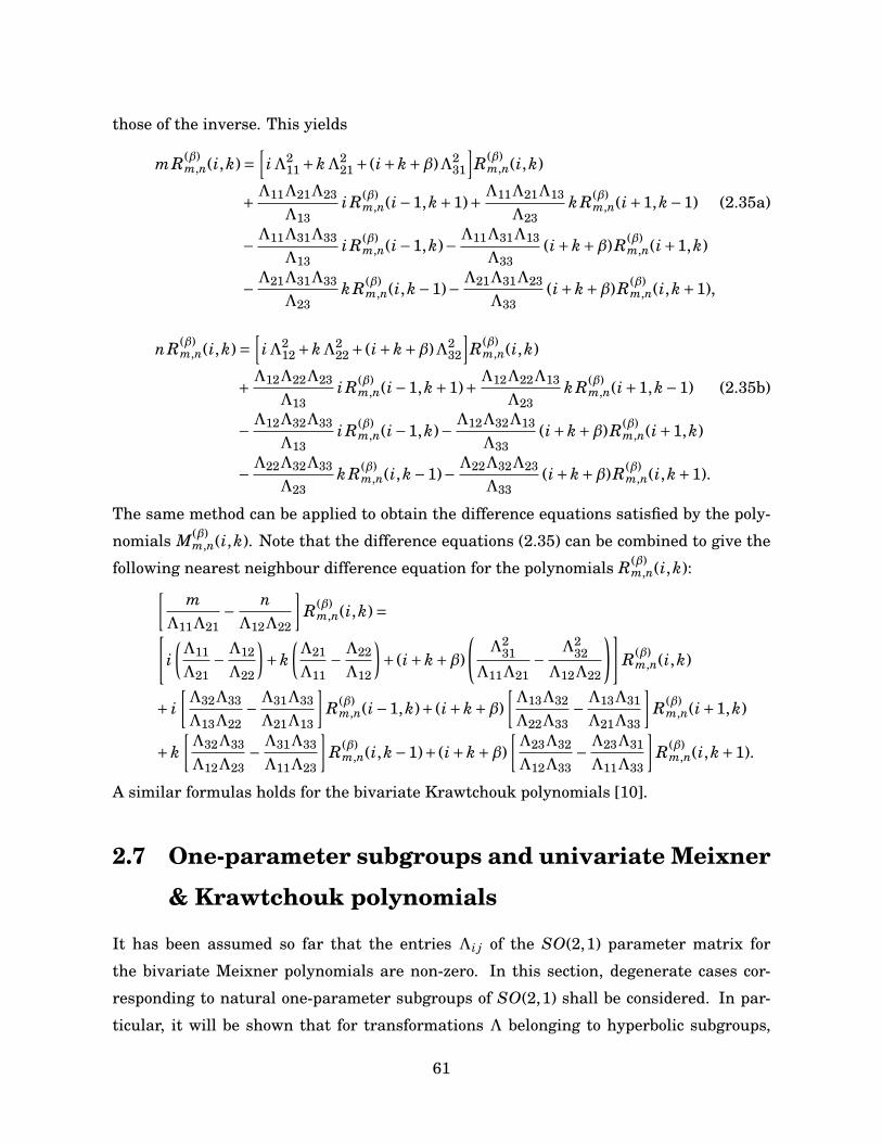
those of the inverse. This yields
mR(β)m,n(i,k)=
[iΛ2
11 +kΛ221 + (i+k+β)Λ2
31
]R(β)
m,n(i,k)
+ Λ11Λ21Λ23
Λ13i R(β)
m,n(i−1,k+1)+ Λ11Λ21Λ13
Λ23k R(β)
m,n(i+1,k−1) (2.35a)
− Λ11Λ31Λ33
Λ13i R(β)
m,n(i−1,k)− Λ11Λ31Λ13
Λ33(i+k+β)R(β)
m,n(i+1,k)
− Λ21Λ31Λ33
Λ23k R(β)
m,n(i,k−1)− Λ21Λ31Λ23
Λ33(i+k+β)R(β)
m,n(i,k+1),
nR(β)m,n(i,k)=
[iΛ2
12 +kΛ222 + (i+k+β)Λ2
32
]R(β)
m,n(i,k)
+ Λ12Λ22Λ23
Λ13i R(β)
m,n(i−1,k+1)+ Λ12Λ22Λ13
Λ23k R(β)
m,n(i+1,k−1) (2.35b)
− Λ12Λ32Λ33
Λ13i R(β)
m,n(i−1,k)− Λ12Λ32Λ13
Λ33(i+k+β)R(β)
m,n(i+1,k)
− Λ22Λ32Λ33
Λ23k R(β)
m,n(i,k−1)− Λ22Λ32Λ23
Λ33(i+k+β)R(β)
m,n(i,k+1).
The same method can be applied to obtain the difference equations satisfied by the poly-
nomials M(β)m,n(i,k). Note that the difference equations (2.35) can be combined to give the
following nearest neighbour difference equation for the polynomials R(β)m,n(i,k):[
mΛ11Λ21
− nΛ12Λ22
]R(β)
m,n(i,k)=[i(Λ11
Λ21− Λ12
Λ22
)+k
(Λ21
Λ11− Λ22
Λ12
)+ (i+k+β)
(Λ2
31
Λ11Λ21− Λ2
32
Λ12Λ22
)]R(β)
m,n(i,k)
+ i[Λ32Λ33
Λ13Λ22− Λ31Λ33
Λ21Λ13
]R(β)
m,n(i−1,k)+ (i+k+β)[Λ13Λ32
Λ22Λ33− Λ13Λ31
Λ21Λ33
]R(β)
m,n(i+1,k)
+k[Λ32Λ33
Λ12Λ23− Λ31Λ33
Λ11Λ23
]R(β)
m,n(i,k−1)+ (i+k+β)[Λ23Λ32
Λ12Λ33− Λ23Λ31
Λ11Λ33
]R(β)
m,n(i,k+1).
A similar formulas holds for the bivariate Krawtchouk polynomials [10].
2.7 One-parameter subgroups and univariate Meixner
& Krawtchouk polynomials
It has been assumed so far that the entries Λi j of the SO(2,1) parameter matrix for
the bivariate Meixner polynomials are non-zero. In this section, degenerate cases cor-
responding to natural one-parameter subgroups of SO(2,1) shall be considered. In par-
ticular, it will be shown that for transformations Λ belonging to hyperbolic subgroups,
61
the matrix elements β⟨ i,k |F (Λ) | m,n ⟩β are given in terms of the standard (univariate)
Meixner polynomials and that for transformations Λ belonging to the elliptic subgroup,
the matrix elements β⟨ i,k |F (Λ) | m,n ⟩β are expressed in terms of standard (univariate)
Krawtchouk polynomials. The one-variable Meixner polynomials Mn(x;δ; c) are defined
by their explicit expression [17]
Mn(x;δ; c)= 2F1
[−n,−xδ
;1− 1c
], (2.36)
where 2F1 is the Gauss hypergeometric function. The monic Meixner polynomials mn(x)
defined through Mn(x;δ; c)= 1(δ)n
( c−1c
)n mn(x) obey the three term recurrence relation
x mn(x)= mn+1(x)+ n+ (n+δ)c1− c
mn(x)+ n(n+δ−1)c(1− c)2 mn−1(x), (2.37)
with m−1(x) = 0 and m0(x) = 1. The one-variable Krawtchouk polynomials are denoted
Kn(x; p; N) and have the expression
Kn(x; p; N)= 2F1
[−n,−x−N
;1p
], (2.38)
where N is a positive integer.
2.7.1 Hyperbolic subgroups: Meixner polynomials
Consider the two hyperbolic one-parameter subgroups of SO(2,1) which have as repre-
sentative elements the following matrices:
Ξ(ξ)=
coshξ 0 sinhξ
0 1 0
sinhξ 0 coshξ
, (2.39a)
Ψ(ψ)=
1 0 0
0 coshψ sinhψ
0 sinhψ coshψ
. (2.39b)
The pseudo-rotations Ξ(ξ) and Ψ(ψ) are unitarily represented by the operators
F (Ξ(ξ))= e−iξK2 , F (Ψ(ψ))= e−iψK1 ,
where K1, K2 are given by (2.5). The matrix elements β⟨ i,k | F (Ξ(ξ)) | m,n ⟩β and
β⟨ i,k | F (Ψ(ψ)) | m,n ⟩β can be evaluated using the approach of Section 3. Let us give
62
the details of the calculation of the matrix elements of F (Ξ(ξ)). Since Ξ(ξ) leaves b2 and
b†2 unaffected and hence acts in a trivial way on the second quantum number, it is readily
seen that
β⟨ i,k |F (Ξ) | m,n ⟩β = δkn β⟨ i |F (Ξ) | m ⟩β,
where the dependence on ξ and on the second quantum number have been suppressed for
notational convenience. Given that
F †(Ξ)b1F (Ξ)= b1 coshξ+b3 sinhξ, F †(Ξ)b†1F (Ξ)= b†
1 coshξ+b†3 sinhξ,
the identity β⟨ i | b†1b1F (Ξ) | m ⟩β = β⟨ i |F (Ξ)F †(Ξ)b†
1b1 F (Ξ) | m ⟩β yields the recurrence
relation
i β⟨ i |F (Ξ) | m ⟩β =[mcosh2 ξ+ (m+γ)sinh2 ξ
]β⟨ i |F (Ξ) | m ⟩β
+coshξsinhξ√
m(m+γ−1)β⟨ i |F (Ξ) | m−1 ⟩β+coshξsinhξ
√(m+1)(m+γ)β⟨ i |F (Ξ) | m+1 ⟩β,
where γ= n+β. Upon taking
β⟨ i |F (Ξ) | m ⟩β = β⟨ i |F (Ξ) | 0 ⟩β√
1m!(γ)m
(coshξsinhξ)−n Pm(i),
where P0(i)= 1, it is seen that Pm(i) satisfies the three-term recurrence relation (2.37) of
the monic Meixner polynomials with c = tanh2 ξ and δ= γ=β+n. One thus has
β⟨ i |F (Ξ) | m ⟩β = β⟨ i |F (Ξ) | 0 ⟩β (−1)m
√(n+β)m
m!tanhm ξMm(i;β+n; tanh2 ξ),
where Mn(x;δ; c) are the univariate Meixner polynomials. There remains to evaluate the
amplitude β⟨ i | F (Ξ) | 0 ⟩β. This can be done using the identity β+1⟨ i | F (Ξ)b1 | 0 ⟩β = 0
which gives the two-term recurrence relation
β⟨ i+1 |F (Ξ) | 0 ⟩β = tanhξ
√i+γi+1 β⟨ i |F (Ξ) | 0 ⟩β,
that has for solution
β⟨ i |F (Ξ) | 0 ⟩β = tanhi ξ
√(γ)i
i! β⟨ 0 |F (Ξ) | 0 ⟩β.
63

Since one has
1= β⟨0 | 0 ⟩β =∑i>0
β⟨ 0 |F †(Ξ) | i ⟩β β⟨ i |F (Ξ) | 0 ⟩β
= ∑i>0
(γ)i
i!tanh2i ξ |β⟨ 0 | F (Ξ) | 0 ⟩β|2,
it follows that
β⟨ i |F (Ξ) | 0 ⟩β =√
(γ)i
i!cosh−γ−i ξsinhi ξ.
The matrix elements of the one-parameter hyperbolic elements Ξ(ξ) are thus given by
β⟨ i,k |F (Ξ(ξ)) | m,n ⟩β
= δkn (−1)m
√(k+β)i(k+β)m
i!m!cosh−k−β ξ tanhi+m ξMm(i;k+β; tanh2 ξ).
(2.40)
In a similar fashion, one obtains for the matrix elements of F (Ψ)
β⟨ i,k |F (Ψ(ψ)) | m,n ⟩β
= δim (−1)n
√(i+β)k(i+β)n
k!n!cosh−i−βψ tanhk+nψMn(k; i+β; tanh2ψ).
(2.41)
2.7.2 Elliptic subgroup: Krawtchouk polynomials
The group SO(2,1) also has a one-parameter elliptic subgroup which has for representa-
tive element the matrix
R(θ)=
cosθ sinθ 0
−sinθ cosθ 0
0 0 1
, (2.42)
which is unitarily represented by F (R(θ))= eiθK3 . The matrix elements
β⟨ i,k |F (R(θ)) | m,n ⟩β,
can be evaluated using the same approach as the one adopted above. Since the details of
similar computations are found in [7], we only give the result which reads
β⟨ i,k |F (R(θ)) | m,n ⟩β
= δi+k,m+n (−1)k
√√√√(i+k
k
)(i+k
n
)cosi+k θ tank+nθKn(k;sin2θ; i+k),
(2.43)
64
where Kn(x; p; N) is given by (2.38) and where(N
i)
stands for the binomial coefficient.
Note that the formula (2.43) does not define proper Krawtchouk polynomials since here
N is not an independent parameter as the variable i+k occurs in its place.
2.8 Addition formulas
In this section, the group product is used to derive a general addition formula for the
bivariate Meixner polynomials.
2.8.1 General addition formula
Let A, B and C be SO(2,1) elements such that C = A ·B with unitary representations
F (A), F (B) and F (C). For a given value of β, to each of these elements is associated
a system of bivariate Meixner polynomials denoted by M(β)m,n(i,k; A), M(β)
m,n(i,k;B) and
M(β)m,n(i,k;C). Since F (C)=F (A)F (B), it follows that
β⟨ i,k |F (C) | m,n ⟩β =∑
ρ,σ>0β⟨ i,k |F (A) | ρ,σ ⟩β β⟨ ρ,σ |F (B) | m,n ⟩β. (2.44)
In terms of the polynomials M(β)m,n(i,k), this identity translates into the addition formulaW (β)
i,k (C)
W (β)i,k (A)
M(β)m,n(i,k;C)= ∑
ρ,σ>0W (β)ρ,σ(B)M(β)
ρ,σ(i,k; A) M(β)m,n(ρ,σ;B). (2.45)
2.8.2 Special case I: product of two hyperbolic elements
Consider the case where the SO(2,1) parameter matrix for the bivariate Meixner polyno-mials R(β)
m,n(i,k) is of the form
Λ=Ψ(ψ) ·Ξ(ξ)=
coshξ 0 sinhξ
sinhξsinhψ coshψ coshξcoshψ
coshψsinhξ sinhψ coshξcoshψ
. (2.46)
In this case the decomposition formula (2.44) can be used to obtain an elegant expression
for the polynomials R(β)m,n(i,k). For the parameter matrix (2.46), one has on the one hand
β⟨ i,k |F (Λ) | m,n ⟩β =√(β)i+k(β)m+n
i!k!m!n!
(Λ13
Λ33
)i (Λ23
Λ33
)k (−Λ31
Λ33
)m (−Λ32
Λ33
)n (1Λ33
)βR(β)
m,n(i,k),(2.47)
65
and on the other hand
β⟨ i,k |F (Λ) | m,n ⟩β =∑
µ,ν>0β⟨ i,k |F (Ψ(ψ)) |µ,ν ⟩ββ⟨µ,ν |F (Ξ(ξ)) | m,n ⟩β. (2.48)
Upon comparing the formulas (2.47) and (2.48) and using the one-parameter matrix ele-
ments (2.40) and (2.41), a direct computation shows that the parameters conspire to yield
the expression
R(β)m,n(i,k)= (i+β)n
(β)nMm(i;n+β; tanh2 ξ)Mn(k; i+β; tanh2ψ). (2.49)
The factorization (2.49) of the bivariate Meixner polynomials as a product of two univari-
ate Meixner polynomials is reminiscent of the bivariate Meixner polynomials defined by
Tratnik. However, the Meixner polynomials (2.49) do not exactly coincide with those de-
fined in [20]. It is seen from (2.34) that in the special case (2.46) one of the recurrence
relations simplifies drastically. Indeed, (2.34) becomes
i R(β)m,n(i,k)=
[mcosh2 ξ+ (m+n+β)sinh2 ξ
]R(β)
m,n(i,k)
−cosh2 ξmR(β)m−1,n(i,k)−sinh2 ξ (m+n+β)R(β)
m+1,n(i,k),
k R(β)m,n(i,k)=
[msinh2 ξsinh2ψ+ncosh2ψ+ (m+n+β)cosh2 ξsinh2ψ
]R(β)
m,n(i,k)
+sinh2ψmR(β)m−1,n+1(i,k)+cosh2ψsinh2 ξnR(β)
m+1,n−1(i,k)
−cosh2 ξsinh2ψmR(β)m−1,n(i,k)−sinh2 ξsinh2ψ (m+n+β)R(β)
m+1,n(i,k)
−cosh2 ξcosh2ψ nR(β)m,n−1(i,k)−sinh2ψ (m+n+β)R(β)
m,n+1(i,k).
The generating function (2.28) also has the simplification
(1− z1 − z2)−β−i−k(1−coth2 ξ z1)i(1− z1 −coth2ψ z2)k
= ∑m,n>0
(β)m+n
m!n!R(β)
m,n(i,k) zm1 zn
2 .
Note that polynomials (2.49) corresponding to the special case (2.46) are orthogonal with
respect to the same weight function (2.19) as the generic polynomials.
2.8.3 General case
Let us now give a formula for the general bivariate Meixner polynomials. The most gen-
eral SO(2,1) pseudo-rotation can be taken of the form
Λ= R(χ)Ψ(ψ)R(θ),
66
where Ψ(ψ) is given by (2.39a) and where R(θ), R(χ) are given by (2.42). For the matrix
Λ, one has again on the one hand
β⟨ i,k |F (Λ) | m,n ⟩β =√(β)i+k(β)m+n
i!k!m!n!
(Λ13
Λ33
)i (Λ23
Λ33
)k (−Λ31
Λ33
)m (−Λ32
Λ33
)n (1Λ33
)βR(β)
m,n(i,k),(2.50)
and on the other hand
β⟨ i,k |F (Λ) | m,n ⟩β == ∑µ,ν,ρ,σ>0
β⟨ i,k |F (R(χ)) |µ,ν ⟩ββ⟨µ,ν |F (Ψ(ψ)) | ρ,σ ⟩ββ⟨ ρ,σ |F (R(θ)) | m,n ⟩β.
(2.51)
Upon comparing the formulas (2.50), (2.51) using the expressions (2.41), (2.43) for the one-variable matrix elements, one arrives at the following formula for the general bivariateMeixner polynomials:
R(β)m,n(i,k)=
(−tan2χ)k(−tan2θ)n ∑µ>0
(−i−k)µ(−n−m)µµ!(β)µ
(tanχtanθsinhψtanhψ)−µ (2.52)
×K i+k−µ(k;sin2χ; i+k)Mm+n−µ(i+k−µ;µ+β; tanh2ψ)Kn(m+n−µ;sin2θ;m+n).
The formula (2.52) thus gives an explicit expression of the bivariate Meixner polynomials
in terms of the Krawtchouk and Meixner polynomials. It is directly seen that the sum-
mation appearing in (2.52) is finite. Moreover, the duality property (2.24) of the bivariate
Meixner polynomials is manifest in (2.52) in view of the duality property of the univariate
Krawtchouk and Meixner polynomials. Note that the comment below (2.43) also applies
for (2.52).
2.9 Multivariate case
In this section, it is shown how the results obtained thus far can easily be general-
ized to d variables by considering the eigenspace of a bilinear expression in the cre-
ation/annihilation operators of d+1 harmonic oscillators.
Consider d+1 pairs of creation and annihilation operators a†i , ai satisfying the Weyl
algebra commutation relations
[ai,ak]= 0, [a†i ,a
†k]= 0, [ai,a
†k]= δik,
67
for i,k = 1, . . . ,d+1 and let H be the Hermitian operator
H = a†1a1 +a†
2a2 +·· ·−a†d+1ad+1. (2.53)
Let β be a positive integer and denote by Vβ be the infinite-dimensional eigenspace asso-
ciated to the eigenvalue 1−β of H. An orthonormal basis for the space Vβ is provided by
the vectors
| n1, . . . ,nd ⟩β =| n1, . . . ,nd, |n|+β−1 ⟩, (2.54)
where the notation |n| = n1+. . .+nd was used. The action of the operators a†i , ai is identical
to the one given in (2.2). Since (2.53) is clearly invariant under SU(d,1) transformations,
it follows that Vβ provides a reducible representation space for the subgroup SO(d,1).
Again, one uses the notation ai = bi for i = 1, . . . ,d and ad+1 = b†d+1.
Let B be a real (d +1)× (d +1) antisymmetric matrix and let Λ be an orthochronous
element of SO(d,1). This means that Λ satisfies
ΛtηΛ= η, Λd+1,d+1 > 1,
where η= diag(1,1, . . . ,−1). Consider now the unitary representation
F (Λ)= exp
(d+1∑i j=1
Bi jb†i b j
), (2.55)
which has for parameters the d(d+1)/2 independent matrix elements of B. The transfor-
mations of the operators bi, b†i under the action of F (Λ) are given by
F (Λ)biF†(Λ)=
d+1∑k=1
Λikbk, F (Λ)b†iF
†(Λ)=d+1∑k=1
Λikb†k,
where Λ denotes the inverse matrix of Λ: ΛΛ= 1. Proceeding in as in Section 4, one can
write the matrix elements of the reducible representations of SO(d,1) on the space Vβ as
follows:
β⟨ x1, . . . , xd |F (Λ) | n1, . . . ,nd ⟩β =W (β)x1,...,xd M(β)
n1,...,nd (x1, . . . , xd),
with M(β)0,...,0(x1, . . . , xd)= 1 and where
W (β)x1,...,xd = β⟨ x1, . . . , xd |F (Λ) | 0, . . . ,0 ⟩β.
68
By considering the identities β+1⟨ x1, . . . , xd |F (Λ)bi | 0, . . . ,0 ⟩β = 0 for i = 1, . . . ,d, one finds
that W (β)x1,··· ,xd is given by
W (β)x1,...,xd =
√(β)|x|
x1! · · ·xd!Λx1
1,d+1Λx22,d+1 · · ·Λ
xdd,d+1Λ
−β−|x|d+1,d+1.
Since
Λ2d+1,d+1 −
d∑i=1Λ2
d+1,i = 1, (2.56)
one has
|W (β)i,k |2 = w(β)
i,k =(β)|x|
x1! · · ·xd!(1−|c|)β cx1
1 · · · cxdd , (2.57)
with
ci =Λ2
i,d+1
Λ2d+1,d+1
, i = 1, . . . ,d
In view of (2.56), the condition |c| < 1 is identically satisfied and hence the following
normalization condition holds:
∑x1,...,xd>0
w(β)x1,...,xd = 1.
The raising relations (2.17) are readily generalized to d variables and from there it is seen
that M(β)n1,...,nd (x1, . . . , xd) are polynomials in the variables x1, . . . , xd of total degree |n|. As
a consequence of the unitarity of the operator F (Λ), the polynomials M(β)n1,...,nd (x1, . . . , xd)
satisfy the orthogonality relation
∑x1,...,xd>0
w(β)x1,...,xd M(β)
n1,...,nd (x1, . . . , xd) M(β)m1,...,md (x1, . . . , xd)= δn1,m1 · · ·δnd ,md , (2.58)
with respect to the negative multinomial distribution (2.57). The calculation of the gen-
erating function of section 5 is also easily generalized to an arbitrary finite number of
variables. One then obtains the generating function used by Griffiths and Iliev to define
the d-variable Meixner polynomials R(β)n1,...,nd (x1, . . . , xd):
(1−|z|)−β−|x|d∏
i=1
(1−
d∑j=1
ui, j z j
)xi
= ∑n1,...,nd>0
(β)|n|n1! · · ·nd!
R(β)n1,...,nd (x1, . . . , xd) zn1
1 · · · zndd .
69
where the parameters ui, j are given by
ui, j =Λi, jΛd+1,d+1
Λi,d+1Λd+1, j,
for i, j = 1, . . . ,d. All properties of the multivariate Meixner polynomials can be derived in
complete analogy with the d = 2 case which has been treated in detail here.
2.10 Conclusion
In summary, we have considered the reducible representations of the SO(d,1) group on
the eigenspace of a bilinear expression in the creation/annihilation operators of d+1 in-
dependent quantum harmonic oscillators. We have shown that the multivariate Meixner
polynomials arise as matrix elements of these SO(d,1) representations and we have seen
that the main properties of the polynomials can be derived systematically using the group
theoretical interpretation.
In [19], the bivariate Krawtchouk polynomials were seen to occur as wavefunctions
of a Hamiltonian describing a discrete/finite model of the harmonic oscillator in two di-
mensions possessing a SU(2) symmetry. This result and the considerations of the present
paper suggest that the bivariate Meixner polynomials could also arise as wavefunctions
of a discrete Hamiltonian. We hope to report on this issue in the future.
References
[1] F. Bergeron. Combinatoire des polynômes orthogonaux classiques: une approche unifiée.
Europ. J. Comb., 11:393–401, 1990.
[2] A. Borodin and G. Olshanski. Meixner polynomials and random partitions. Moscow Math. J.,
6:629–655, 2006.
[3] P. Diaconis and R. C. Griffiths. An introduction to multivariate Krawtchouk polynomials and
their applications. J. Stat. Plan. Inf., 154:39–53, 2014.
[4] R. Floreanini, J. LeTourneux, and L. Vinet. Quantum Mechanics and Polynomials of a Dis-
crete Variable. Ann. Phys., 226:331–349, 1993.
[5] D. Foata and J. Labelle. Modèles Combinatoires pour les Polynômes de Meixner. Europ. J.
Comb., 4:305–311, 1983.
70
[6] V. X. Genest, L. Vinet, and A. Zhedanov. Interbasis expansions for the isotropic 3D harmonic
oscillator and bivariate Krawtchouk polynomials. J. Phys. A: Math. Theor., 47:025202, 2013.
[7] V. X. Genest, L. Vinet, and A. Zhedanov. The multivariate Krawtchouk polynomials as matrix
elements of the rotation group representations on oscillator states. J. Phys. A: Math. Theor.,
46:505203, 2013.
[8] R. C. Griffiths. Orthogonal Polynomials on the Multinomial Distribution. Aus. J. Stat., 13:27–
35, 1971.
[9] R. C. Griffiths. Orthogonal Polynomials on the Negative Multinomial Distribution. J. Mult.
Var. Anal., 54:271–277, 1975.
[10] A. Grünbaum. The Rahman Polynomials Are Bispectral. SIGMA, 302:65–75, 2007.
[11] A. Grünbaum and M. Rahman. A System of Multivariable Krawtchouk polynomials and a
Probabilistic Application. SIGMA, 7:119–135, 2011.
[12] P. Iliev. Meixner polynomials in several variables satisfying bispectral difference equations.
Adv. Appl. Math., 49:15–23, 2012.
[13] K. Johansson. Shape fluctuations and random matrices. Comm. Math. Phys., 209:437–476,
2000.
[14] K. Johansson. Discrete orthogonal polynomial ensembles and the Plancherel measure. Ann.
Math., 153:259–296, 2001.
[15] S. Karlin and J. McGregor. The classification of birth and death processes. Trans. Amer.
Math. Soc., 86:366–400, 1957.
[16] S. Karlin and J. McGregor. Linear Growth, Birth and Death Processes. J. Math. Mech.,
7:643–662, 1958.
[17] R. Koekoek, P.A. Lesky, and R.F. Swarttouw. Hypergeometric orthogonal polynomials and
their q-analogues. Springer, 1st edition, 2010.
[18] J. Meixner. Orthogonale Polynomsysteme mit einer besonderen Gestalt der erzeugenden
Funktion. J. London Math. Soc., s1-9:6–13, 1934.
[19] H. Miki, S. Post, L. Vinet, and A. Zhedanov. A superintegrable finite oscillator in two dimen-
sions with SU(2) symmetry. J. Phys. A: Math. Theor., 46:125207, 2012.
[20] M. V. Tratnik. Some multivariable orthogonal polynomials of the Askey tableau-discrete
families. J. Math. Phys., 32:2337, 1991.
71

[21] N. Ja. Vilenkin and A. U. Klimyk. Representation of Lie Groups and Special Functions.
Kluwer Academic Publishers, 1991.
72
Chapitre 3
The multivariate Charlierpolynomials as matrix elements of theEuclidean group representation onoscillator states
V. X. Genest, H. Miki, L. Vinet et A. Zhedanov (2014). The multivariate Charlier polynomials as
matrix elements of the Euclidean group representation on oscillator states. Journal of Physics A:
Mathematical and Theoretical 47 215204
Abstract. A family of multivariate orthogonal polynomials generalizing the standard (univari-
ate) Charlier polynomials is shown to arise in the matrix elements of the unitary representation
of the Euclidean group E(d) on oscillator states. These polynomials in d discrete variables are
orthogonal on the product of d Poisson distributions. The accent is put on the d = 2 case and the
group theoretical setting is used to obtain the main properties of the polynomials: orthogonality
and recurrence relations, difference equation, raising/lowering relations, generating function, hy-
pergeometric and integral representations and explicit expression in terms of standard Charlier
and Krawtchouk polynomials. The approach is seen to extend straightforwardly to an arbitrary
number of variables. The contraction of SO(3) to E(2) is used to show that the bivariate Charlier
polynomials correspond to a limit of the bivariate Krawtchouk polynomials.
73
3.1 Introduction
In this paper, a new family of multi-variable Charlier polynomials that arise as matrix elements
of the unitary reducible Euclidean group representation on oscillator states is introduced. The
main properties of these polynomials are obtained naturally from the group theoretical context.
The focus is put mainly on the bivariate case, for which the two-variable Charlier polynomials
occur in the matrix elements of unitary reducible E(2) representations on the eigenstates of a two-
dimensional isotropic harmonic oscillator. The extension to an arbitrary number of variables is
straightforward and is given towards the end of the paper.
The standard Charlier polynomials Cn(x;a) of degree n in the variable x were introduced in
1905 [2]. These polynomials form one of the most elementary family of orthogonal polynomials
(OPs) in the Askey scheme of hypergeometric OPs [17]. They are orthogonal with respect to the
Poisson distribution w(a)x with parameter a > 0 which is defined by
w(a)x = axe−a
x!,
and their discrete orthogonality relation reads
∞∑x=0
w(a)x Cn(x;a)Cm(x;a)= a−nn!δnm.
They can be defined through their generating function
et(1− t
a
)x=
∞∑n=0
Cn(x;a)n!
tn, (3.1)
and can be expressed in terms of a 2F0 hypergeometric function (see [17] for additional properties
and references). The Charlier polynomials appear in various fields including combinatorics [18]
as well as statistics and probability [9, 19]. In Physics, the importance of these polynomials is
mostly due to their appearance in the matrix elements of unitary irreducible representations of
the one-dimensional oscillator group [10, 21].
In a recent series of papers [6, 7, 8], we have presented group theoretical interpretations for
two families of multivariate orthogonal polynomials: the multi-variable Krawtchouk and Meixner
polynomials. These two families, introduced by Griffiths in [11, 12], were seen to occur in the
matrix elements of reducible unitary representations of the rotation and pseudo-rotation groups on
oscillator states. This algebraic framework led to a number of new identities for these polynomials
and allowed for simple derivations of their known properties.
Here we consider the Euclidean group E(d) which is the group generated by the translations
and the rotations in d-dimensional Euclidean space. We shall investigate the matrix elements of
the unitary reducible representation of this group on the eigenstates of a d-dimensional isotropic
74
harmonic oscillator and show that these are expressed in terms of a new family of multivariate
orthogonal polynomials that shall be identified as multivariate extensions of the standard Charlier
polynomials. The main properties of these polynomials will be derived in a simple fashion using
the group theoretical interpretation.
The paper is organized as follows. In section 2, the unitary representations of the Euclidean
group E(2) are defined. In section 3, it is shown that the matrix elements of these representations
are given in terms of bivariate polynomials that are orthogonal with respect to the product of
two (independent) Poisson distributions. The duality relation satisfied by these polynomials is
discussed in section 4. In section 5, a generating function is obtained and the polynomials are
identified as multivariate Charlier polynomials. The generating function is used in section 6 to
find an explicit expression for these Charlier polynomials in terms of generalized hypergeometric
series. The recurrence relations and the difference equations are given in section 7. In section 8,
the matrix elements for one-parameter subgroups are considered and used to obtain an explicit
expression for the bivariate Charlier polynomials in terms of standard Charlier and Krawtchouk
polynomials. In section 9, an integral representation is given. In section 10, it is shown that
the bivariate Charlier polynomials can be obtained from the bivariate Krawtchouk polynomials
through a limit process. In section 11, the d-dimensional case is treated. A conclusion follows.
3.2 Unitary representations of E(2) on oscillator states
In this section, the reducible unitary representation of the Euclidean group that shall be used
throughout the paper is defined. This representation will be specified on the eigenstates of the
two-dimensional isotropic harmonic oscillator.
3.2.1 The Heisenberg-Weyl algebra
Let ai, a†i , i = 1, 2, be the generators of the Heisenberg-Weyl algebra satisfying the commutation
relations
[ai,a†j]= δi j, [ai,a j]= 0, [a†
i ,a†j]= 0. (3.2)
This algebra has a standard representation on the basis vectors
| n1,n2 ⟩ ≡| n1 ⟩⊗| n2 ⟩, n1,n2 = 0,1, . . . ,
defined by the actions of the generators on the factors of the direct product:
ai| ni ⟩ =pni | ni −1 ⟩, a†
i | ni ⟩ =√
ni +1 | ni +1 ⟩. (3.3)
75
In view of the commutation relations (3.2) and the actions (3.3), the basis vectors | n1,n2 ⟩ can
equivalently be written as
| n1,n2 ⟩ =(a†
1)n1(a†2)n2√
n1!n2!| 0,0 ⟩. (3.4)
In Cartesian coordinates, the algebra (3.2) has the following realization:
ai = 1p2
(xi + ∂
∂xi
), a†
i =1p2
(xi − ∂
∂xi
), i = 1,2. (3.5)
3.2.2 The two-dimensional isotropic oscillator
Consider the Hamiltonian H governing the isotropic harmonic oscillator in the two-dimensional
Euclidean space
H =−12
(∂2
∂x21+ ∂2
∂x22
)+ 1
2(x2
1 + x22). (3.6)
Using the realization (3.5), the Hamiltonian (3.6) can be written as
H = a†1a1 +a†
2a2 +1. (3.7)
It is seen from (3.3) that the Hamiltonian (3.7) is diagonal on the basis vectors | n1,n2 ⟩ with energy
eigenvalue E given by:
H | n1,n2 ⟩ = E| n1,n2 ⟩, E = n1 +n2 +1.
The Schrödinger equation HΨ= EΨ associated to the Hamiltonian (3.6) separates in the Carte-
sian coordinates x1, x2. In these coordinates, the wavefunctions take the form
⟨ x1, x2 | n1,n2 ⟩ =Ψn1(x1)Ψn2(x2),
with
⟨ xi | ni ⟩ =Ψni (xi)=√
12ni π1/2 ni!
e−x2i /2Hni (xi), (3.8)
where Hn(x) denotes the Hermite polynomials [17]. The wavefunctions Ψni (xi) satisfy the orthog-
onality relation∫ ∞
−∞Ψni (xi)Ψn′
i(xi)dxi = δni n′
i. (3.9)
76
3.2.3 The representation of E(2) on oscillator states
The eigenstates of the two-dimensional quantum harmonic oscillator support a reducible repre-
sentation of the Euclidean group E(2). We introduce the following notation for the basis vectors:
| m,n ⟩ ≡| n1,n2 ⟩,
so that m and n are identified with n1 and n2, respectively. The E(2) group is generated by two
translation operators in the x1 and x2 directions given by
P1 = i(a1 −a†1), P2 = i(a2 −a†
2), (3.10)
and by a rotation generator J which has the expression
J = i(a1a†2 −a†
1a2). (3.11)
The generators P1, P2 and J satisfy the commutation relations of the Euclidean Lie algebra e(2)
which read
[P1,P2]= 0, [P2, J]= iP1, [J,P1]= iP2. (3.12)
Using the formulas (3.3), the actions of the Euclidean generators defined by (3.10) and (3.11)
on the eigenstates of the two-dimensional oscillator are easily obtained. The assertion that this
representation of the Euclidean group is reducible follows from the observation that the Casimir
operator C of e(2), which can be written as
C = P21 +P2
2 ,
does not act, as is directly checked, as a multiple of the identity on | m,n ⟩.We use the following notation. Let T(θ,α,β) be a generic element of the Euclidean group E(2)
where θ, α and β are real parameters; T(θ,α,β) can be written as
T(θ,α,β)=
cosθ sinθ α/
p2
−sinθ cosθ β/p
2
0 0 1
,
and represents the Euclidean move
(x1, x2,1)> → T(θ,α,β)(x1, x2,1)>,
where z> stands for transposition. The group multiplication law is provided by the standard
matrix product. Consider the unitary representation defined by
U(T)= eiαP1 eiβP2 eiθJ . (3.13)
77
It is readily checked that U(T)U†(T) = 1. The transformations of the generators ai, a†i under the
action of U(T) is given by
U(T)a1U†(T)= cosθa1 −sinθa2 −αcosθ+βsinθ,
U(T)a2U†(T)= sinθa1 +cosθa2 −αsinθ−βcosθ,(3.14)
Similar formulas involving a†1 and a†
2 are obtained by taking the complex conjugate of (3.14). Since
one has X i = 2−1/2(ai +a†i ), i = 1,2, the transformation laws (3.14) give for the coordinate operator
(X1, X2)X1
X2
=U(T)
X1
X2
U†(T)=cosθ −sinθ
sinθ cosθ
X1
X2
+A
B
, (3.15)
where
A =− 2p2
(αcosθ−βsinθ
), B =− 2p
2
(αsinθ+βcosθ
). (3.16)
One thus has
U†(T)| x1, x2 ⟩ =| x1, x2 ⟩ =| T−1x1,T−1x2 ⟩,
where x1, x2 are given byx1
x2
=cosθ −sinθ
sinθ cosθ
x1
x2
+A
B
, (3.17)
with A, B given by (3.16). Moreover, one has U(TT ′) =U(T)U(T ′) as should be for a group repre-
sentation. The inverse transformation formulas
U†(T)a1U(T)= cosθa1 +sinθa2 +α,
U†(T)a2U(T)=−sinθa1 +cosθa2 +β.(3.18)
and the Glauber formula [3]:
eγ (a†i−ai) = e−γ
2/2eγa†i e−γai , i = 1,2, (3.19)
shall also prove useful in what follows.
3.3 The representation matrix elements as orthogonal
polynomials
In this section it is shown that the matrix elements of the unitary representation of E(2) defined
in section 2 are expressed in terms of bivariate orthogonal polynomials. The matrix elements of
78

U(T) defined by (3.13) can be written as
⟨ i,k |U(T) | m,n ⟩ =Wi,k Cm,n(i,k), (3.20)
where C0,0(i,k)= 1 and where Wi,k is defined by
Wi,k = ⟨ i,k |U(T) | 0,0 ⟩. (3.21)
To ease the notation, the explicit dependence of U(T) on T shall be dropped.
3.3.1 Calculation of Wi,k
The amplitude Wi,k can evaluated by a direct computation. Indeed, since one has eiθJ | 0,0 ⟩ =| 0,0 ⟩,it follows that
Wi,k = ⟨ i,k | eiαP1 eiβP2 eiθJ | 0,0 ⟩ = ⟨ i,k | eiαP1 eiβP2 | 0,0 ⟩.
Upon using the Glauber formula (3.19) to write
eiαP1 = eα(a†1−a1) = e−α
2/2eαa†1 e−αa1 , eiβP2 = eβ(a†
2−a2) = e−β2/2eβa†
2 e−βa2 ,
and the actions (3.3), one easily finds
Wi,k = e−(α2+β2)/2 αiβk
pi!k!
. (3.22)
3.3.2 Raising relations
It will now be shown that the functions Cm,n(i,k) that appear in the matrix elements (3.20) are
polynomials of total degree m+ n in the discrete variables i,k. This will be done by exhibiting
raising relations for Cm,n(i,k). Consider the matrix element ⟨ i,k |Ua†1 | m,n ⟩. One has on the one
hand
⟨ i,k |Ua†1 | m,n ⟩ =
pm+1Wi,k Cm+1,n(i,k), (3.23)
and on the other hand, using (3.14), one has
⟨ i,k |Ua†1 | m,n ⟩ = ⟨ i,k |Ua†
1U†U | m,n ⟩ = cosθp
iWi−1,kCm,n(i−1,k)
−sinθp
kWi,k−1Cm,n(i,k−1)+ (βsinθ−αcosθ)Wi,kCm,n(i,k). (3.24)
Upon comparing (3.23) and (3.24), one obtains using (3.22)
pm+1Cm+1,n(i,k)=
(iα
)cosθCm,n(i−1,k)
−(
kβ
)sinθCm,n(i,k−1)+ (βsinθ−αcosθ)Cm,n(i,k).
(3.25)
79
Considering instead the matrix element ⟨ i,k |Ua†2 | m,n ⟩, one similarly finds
pn+1Cm,n+1(i,k)=
(iα
)sinθCm,n(i−1,k)
+(
kβ
)cosθCm,n(i,k−1)− (αsinθ+βcosθ)Cm,n(i,k).
(3.26)
By definition one has C−1,n(i,k)= Cm,−1(i,k)= 0 and C0,0(i,k)= 1. As a consequence, the formulas
(3.25) and (3.26) can be used to construct Cm,n(i,k) from C0,0(i,k) iteratively. One then observes
that Cm,n(i,k) are polynomials of total degree m+n in the (discrete) variables i,k.
3.3.3 Orthogonality relation
The unitarity of the representation (3.13) and the orthonormality of the basis states leads to an
orthogonality relation for the polynomials Cm,n(i,k). One has
⟨ m′,n′ |U†U | m,n ⟩ =∞∑
i,k=0⟨ i,k |U | m,n ⟩⟨ m′,n′ |U† | i,k ⟩ = δmm′δnn′ .
Upon using (3.20) and the reality of the matrix elements in the above equation, the following
orthogonality relation is obtained:
∞∑i,k=0
wi,k Cm,n(i,k)Cm′,n′(i,k)= δmm′δnn′ , (3.27)
where wi,k is the product of two independent Poisson distributions with (positive) parameters α2
and β2:
wi,k =W2i,k = e−(α2+β2)α
2iβ2k
i!k!. (3.28)
3.3.4 Lowering relations
Lowering relations for the polynomials Cm,n(i,k) can be obtained by considering the matrix el-
ements ⟨ i,k | Uai | m,n ⟩, i = 1,2 and proceeding as for the raising relations. From the matrix
element ⟨ i,k |Ua1 | m,n ⟩, one finds
pmCm−1,n(i,k)=αcosθCm,n(i+1,k)
−βsinθCm,n(i,k+1)+ (βsinθ−αcosθ)Cm,n(i,k).
From the matrix element ⟨ i,k |Ua2 | m,n ⟩, one obtains
pnCm,n−1(i,k)=αsinθCm,n(i+1,k)
+βcosθCm,n(i,k+1)− (αsinθ+βcosθ)Cm,n(i,k).
80
3.4 Duality
In this section, a duality relation under the exchange of the variables i,k and the degrees m,n in
the polynomials Cm,n(i,k) is obtained. Consider the matrix elements ⟨ i,k |U† | m,n ⟩ and write
⟨ i,k |U† | m,n ⟩ = Wi,kCm,n(i,k), (3.29)
where C0,0(i,k) = 1 and Wi,k = ⟨ i,k |U† | 0,0 ⟩. To evaluate the amplitude Wi,k, one first observes
that the identity ⟨ i,k |U†ai | 0,0 ⟩ = 0 holds for i = 1,2. Using the inverse transformation formulas
(3.18), one obtains the following system of difference equation
cosθp
i+1Wi+1,k +sinθp
k+1Wi,k+1 +αWi,k = 0,
−sinθp
i+1Wi+1,k +cosθp
k+1Wi,k+1 +βWi,k = 0.
It is easily seen that the solution of this system is given by
Wi,k = C(βsinθ−αcosθ)i(−αsinθ−βcosθ)k
pi!k!
,
where C is a constant. The value of C can be determined by the normalization condition
1= ⟨ 0,0 |U†U | 0,0 ⟩ =∞∑
i,k=0⟨ i,k |U† | 0,0 ⟩⟨ 0,0 |U | i,k ⟩ =
∞∑i,k=0
|Wi,k|2,
which gives C2 = e−(αcosθ−βsinθ)2e−(αsinθ+βcosθ)2 = e−(α2+β2) and thus
Wi,k = e−(α2+β2)/2 (βsinθ−αcosθ)i(−αsinθ−βcosθ)kp
i!k!. (3.30)
Note that Wi,k can also be computed directly (see section 5). Since U†(T) =U(T−1), the Cm,n(i,k)
are the polynomials corresponding to the inverse transformation T−1. For a transformation T ∈E(2) specified by the parameters (θ,α,β), the inverse T−1 ∈ E(2) is specified by the parameters
(θ, α, β) given by
θ =−θ, α= (βsinθ−αcosθ), β=−(αsinθ+βcosθ). (3.31)
One can also obtain the matrix element (3.29) by
⟨ i,k |U† | m,n ⟩ = ⟨ m,n |U | i,k ⟩∗ = ⟨ m,n |U | i,k ⟩ =Wm,nCi,k(m,n), (3.32)
where the reality of the matrix elements (3.20) has been used. Upon combining (3.29) and (3.32),
one finds that
Ci,k(m,n)=√
m!n!i!k!
(αiβk
αmβn
)Cm,n(i,k), (3.33)
81
where Cm,n(i,k) corresponds to the polynomial Cm,n(i,k) with parameters (θ, α, β) given by (3.31).
For the two variable polynomials Sm,n(i,k) defined by
Cm,n(i,k)= (−1)n+mp
m!n!(αcosθ−βsinθ)m(αsinθ+βcosθ)nSm,n(i,k), (3.34)
the duality relation (3.33) takes the elegant form
Si,k(m,n)= Sm,n(i,k).
3.5 Generating function
In this section, a generating function for the bivariate orthogonal polynomials Cm,n(i,k) is ob-
tained and is seen to correspond to a multivariate extension of that of the standard Charlier
polynomials. Consider the generating series
F(x, y)=∞∑
m,n=0Wi,kCm,n(i,k)
xm ynp
m!n!=
∞∑m,n=0
⟨ i,k |U | m,n ⟩ xm ynp
m!n!. (3.35)
Using the expression (3.4) for the basis vectors | n1,n2 ⟩ and the transformation formulas (3.14),
one has
F(x, y)=∞∑
m,n=0
xm ynp
m!n!⟨ i,k |U (a†
1)m
pm!
(a†2)n
pn!
| 0,0 ⟩ =∞∑
m,n=0⟨ i,k |U (xa†
1)m(ya†2)n
m!n!| 0,0 ⟩
= ⟨ i,k |Uexa†1 eya†
2 | 0,0 ⟩ = ⟨ i,k |Uexa†1U†Ueya†
2U†U | 0,0 ⟩= ⟨ i,k | exUa†
1U†eyUa†
2U†U | 0,0 ⟩
= e−x(αcosθ−βsinθ)e−y(αsinθ+βcosθ)⟨ i,k | ea†1(xcosθ+ysinθ)ea†
2(ycosθ−xsinθ)U | 0,0 ⟩.
(3.36)
Since one has U | 0,0 ⟩ = e−(α2+β2)/2eαa†1 eβa†
2 | 0,0 ⟩ by the Glauber formula (3.19) and by the actions
(3.3), one finds
F(x, y)= e−(α2+β2)/2
× e−x(αcosθ−βsinθ)e−y(αsinθ+βcosθ)⟨ i,k | ea†1(α+xcosθ+ysinθ)ea†
2(β+ycosθ−xsinθ) | 0,0 ⟩,
which gives
F(x, y)= e−(α2+β2)/2
× e−x(αcosθ−βsinθ)e−y(αsinθ+βcosθ) (α+ xcosθ+ ysinθ)i(β+ ycosθ− xsinθ)kp
i!k!.
82
Recalling the expression (3.22) for Wi,k, the following generating function for the polynomials
Cm,n(i,k) is obtained:
e−x(αcosθ−βsinθ)e−y(αsinθ+βcosθ)[1+ x
αcosθ+ y
αsinθ
]i[1− x
βsinθ+ y
βcosθ
]k
=∞∑
m,n=0Cm,n(i,k)
xm ynp
m!n!.
(3.37)
For the polynomials Sm,n(i,k) given by (3.34), defining
z1 =−x(αcosθ−βsinθ)x, z2 =−y(αsinθ+βcosθ),
yields the generating function
ez1+z2 [1+u11z1 +u12z2]i [1+u21z1 +u22z2]k =∞∑
m,n=0
Sm,n(i,k)m!n!
zm1 zn
2 (3.38)
where the parameters ui j are of the form
u11 = −cosθα2 cosθ−αβsinθ
, u12 = −sinθα2 sinθ+αβcosθ
,
u21 = −sinθβ2 sinθ−αβcosθ
, u22 = −cosθβ2 cosθ+αβsinθ
.(3.39)
The expression (3.38) for the generating function of the polynomials Sm,n(i,k) lends itself to com-
parison with that of the Charlier polynomials (3.1). It is clear from this that Sm,n(i,k) can be
identified with multivariate Charlier polynomials.
3.6 Explicit expression in hypergeometric series
In this section, an explicit expression for the bivariate Charlier polynomials Sm,n(i,k) in terms of a
Gelfan’d-Aomoto hypergeometric series is obtained. Consider the generating relation (3.38). Upon
denoting by F(z1, z2) the left-hand side of (3.38) and using the trinomial expansion, one finds
F(z1, z2)= ez1+z2∑
ρ,σ,µ,ν
(iρ
)(i−ρσ
)(kµ
)(k−µν
)uρ11uσ12uµ21uν22 zρ+µ1 zσ+ν2 , (3.40)
where the summation runs over all non-negative values of the indices and where binomial co-
efficients with negative entries are taken to be zero. Upon expanding the exponential in (3.40),
gathering the terms in zm1 zn
2 and using the identity (−1)nm!(m−n)! = (−m)n where (a)n stands for the
Pochhammer symbol
(a)n = a(a+1) · · · (a+n−1), (a)0 = 1,
83
one finds that the bivariate Charlier polynomials can be written as
Sm,n(i,k)= ∑ρ,σ,µ,ν
(−m)ρ+µ(−n)ν+σ(−i)ρ+σ(−k)µ+νρ!σ!µ!ν!
uρ11uσ12uµ21uν22, (3.41)
where the ui j are given by (3.39). The series appearing in (3.41) is a special case of Gelfan’d-
Aomoto hypergeometric series [1, 5]. The multivariate orthogonal polynomials of Krawtchouk
and Meixner type are also known to admit explicit expressions in terms of these multi-variable
generalized hypergeometric series (see [13] and [14]).
3.7 Recurrence relations and difference equations
In this section, the group theoretical framework is exploited to obtain the bispectral properties of
the bivariate Charlier polynomials Cm,n(i,k).
3.7.1 Recurrence relations
A pair of recurrence relations for the bivariate Charlier polynomials can be obtained by examining
the matrix elements ⟨ i,k | a†i aiU | m,n ⟩ for i = 1,2. Consider the case i = 1 first, one has on the
one hand
⟨ i,k | a†1a1U | m,n ⟩ = iWi,k Cm,n(i,k). (3.42)
On the other hand, using the unitary of U , one has
⟨ i,k | a†1a1U | m,n ⟩ = ⟨ i,k |U U†a†
1U U†a1U | m,n ⟩. (3.43)
Comparing (3.42) with (3.43) using the transformation rules (3.18), one obtains the recurrence
relation
i Cm,n(i,k)= [mcos2θ+nsin2θ+α2]
Cm,n(i,k)
+αsinθ[p
n+1Cm,n+1(i,k)+pnCm,n−1(i,k)
]+sinθ cosθ
√n(m+1)Cm+1,n−1(i,k)
+αcosθ[p
m+1Cm+1,n(i,k)+pmCm−1,n(i,k)
]+sinθ cosθ
√m(n+1)Cm−1,n+1(i,k).
In a similar fashion, one finds from the matrix element ⟨ i,k | a†2a2U | m,n ⟩ a second recurrence
relation
kCm,n(i,k)= [msin2θ+ncos2θ+β2]
Cm,n(i,k)
+βcosθ[p
n+1Cm,n+1(i,k)+pnCm,n−1(i,k)
]−sinθ cosθ
√n(m+1)Cm+1,n−1(i,k)
−βsinθ[p
m+1Cm+1,n(i,k)+pmCm−1,n(i,k)
]−sinθ cosθ
√m(n+1)Cm−1,n+1(i,k).
84
3.7.2 Difference equations
A pair of difference equations can be obtained by considering instead the matrix elements
⟨ i,k |Ua†i ai | m,n ⟩
for i = 1,2. Taking i = 1, one has
⟨ i,k |Ua†1a1 | m,n ⟩ = mWi,k Cm,n(i,k).
Comparing the above relation with ⟨ i,k |Ua†1a1 | m,n ⟩ = ⟨ i,k |Ua†
1U† Ua1U†U | m,n ⟩ using the
transformation formulas (3.14), one obtains
mCm,n(i,k)= [i cos2θ+ksin2θ+ω2]
Cm,n(i,k)
−ωcosθ[
iα
Cm,n(i−1,k)+αCm,n(i+1,k)]− iβα
cosθsinθCm,n(i−1,k+1)
+ωsinθ[
kβ
Cm,n(i,k−1)+βCm,n(i,k+1)]− kα
βcosθsinθCm,n(i+1,k−1),
where ω=αcosθ−βsinθ. Starting instead from ⟨ i,k |Ua†2a2 | m,n ⟩, one similarly finds
nCm,n(i,k)= [i sin2θ+kcos2θ+ζ2]
Cm,n(i,k)
−ζsinθ[
iα
Cm,n(i−1,k)+αCm,n(i+1,k)]+ iβα
cosθsinθCm,n(i−1,k+1)
−ζcosθ[
kβ
Cm,n(i,k−1)+βCm,n(i,k+1)]+ kα
βcosθsinθCm,n(i+1,k−1),
with ζ=αsinθ+βcosθ.
3.8 Explicit expression in standard
Charlier and Krawtchouk polynomials
In this section, an explicit expression for the bivariate Charlier polynomials Cm,n(i,k) involving
the standard (univariate) Charlier and Krawtchouk polynomials. To this end, one first notes that
the matrix elements ⟨ i,k |U | m,n ⟩ can be decomposed as follows:
⟨ i,k |U | m,n ⟩ =∞∑
r,s,u,v=0⟨ i,k | eiP1 | r, s ⟩⟨ r, s | eiβP2 | u,v ⟩⟨ u,v | eiθJ | m,n ⟩. (3.44)
We shall now examine individually the matrix elements appearing in the right hand side of the
above equation.
85
Consider the matrix element ⟨ i,k | eiαP1 | r, s ⟩ which corresponds to a translation in the x1
direction. Since P1 acts only on the first quantum number, one has
⟨ i,k | eiαP1 | r, s ⟩ = δks⟨ i,k | eαP1 | r,k ⟩.
The expression for the above matrix element is well known (see for example [22] or [21]) and can
be obtained directly by taking β = 0 in the formula (3.22) for the amplitude Wi,k and by taking
θ =β= y= 0 in the generating function (3.37). Comparing with (3.1), one finds that
⟨ i,k | eiαP1 | r, s ⟩ = δks(−1)rαr+i
pi!r!
e−α2/2Cr(i;α2), (3.45)
where Cn(x;a) are the standard Charlier polynomials [17]. Similarly, one has
⟨ r, s | eiβP2 | u,v ⟩ = δru(−1)vβv+sp
s!v!e−β
2/2Cv(s;β2). (3.46)
The matrix element ⟨ u,v | eiθJ | m,n ⟩ can be evaluated straightforwardly using the methods of
[6, 7]. The result reads
⟨ u,v | eiθJ | m,n ⟩ = δu+v,m+n(−1)v
(Nv
)1/2(Nn
)1/2
cosN θ tanv+n θKn(v;sin2θ; N) (3.47)
where u+ v = m+n = N and where Kn(x; p; N) stands for the standard Krawtchouk polynomials
[17]. Upon using the matrix elements (3.45), (3.46) and (3.47) in the decomposition formula (3.44)
and using the formula (3.22), one finds that the bivariate Charlier polynomials Cm,n(i,k) are given
by
Cm,n(i,k)= (−1)n+mαm+n cosm θsinn θpm!n!
m+n∑v=0
(m+n
v
)(−βsinθαcosθ
)vCv(k;β2)Cm+n−v(i;α2)Kn(v;sin2θ,n+m), (3.48)
where Cn(x;a) and Kn(x; p; N) are the standard Charlier and Krawtchouk polynomials.
3.9 Integral representation
An integral representation for the bivariate Charlier polynomials can be obtained by considering
the matrix element ⟨ x1, x2 |U | m,n ⟩ from two different points of view. First, consider the action
of U on | m,n ⟩. Using the definition (3.20) of the matrix elements, one can write
⟨ x1, x2 |U | m,n ⟩ =∞∑
i,k=0Wi,kCm,n(i,k)Ψi(x1)Ψk(x2),
86
where Ψni (xi), i = 1,2, is given by (3.8). Second, take the action of U on the bra ⟨ x1, x2 ||. In view
of (3.17), one may write
⟨ x1, x2 |U | m,n ⟩ = ⟨ x1, x2 | m,n ⟩ =Ψm(x1)Ψn(x2),
where (x1, x2) is given by (3.17). Combining the two previous relations, there comes
Ψm(x1)Ψn(x2)=∞∑
i,k=0Wi,k Cm,n(i,k)Ψi(x1)Ψk(x2).
Upon multiplying both sides of the above equation by Ψi′(x1)Ψk′(x2), integrating over the whole
Euclidean plane and using the orthogonality relation (3.9) for the wavefunctions, one finds that
Cm,n(i,k)= 1Wi,k
∫ ∞
−∞
∫ ∞
−∞Ψi(x1)Ψk(x2)Ψm(x1)Ψn(x2)dx1dx2,
with (x1, x2) given by (3.17). In view of (3.8), this gives a formula for the bivariate Charlier poly-
nomials Cm,n(i,k) in terms of a double integral of a product of four Hermite polynomials.
3.10 Charlier polynomials as limits of
Krawtchouk polynomials
In this section, it is shown that the bivariate Charlier polynomials Cm,n(i,k) can be obtained from
the bivariate Krawtchouk polynomials by a limit process. We begin by providing some background
information on the bivariate Krawtchouk polynomials.
3.10.1 Bivariate Krawtchouk polynomials
The bivariate Krawtchouk polynomials Pm,n(i,k; N) of two discrete variables i, k arise as matrix
elements of the rotation group SO(3) on the energy E = N +3/2 eigenspace of a three-dimensional
isotropic harmonic oscillator [7]. In addition to the non-negative integer N, the bivariate Kraw-
tchouk polynomials have for parameters the entries of a rotation matrix R ∈ SO(3). Hence for
each N and R ∈ SO(3), one has a finite set of bivariate Krawtchouk polynomials. The polynomials
Pm,n(i,k; N) can be defined through the following generating function:
G(u,v)=(1+ R11
R13u+ R12
R13v)i (
1+ R21
R23u+ R22
R23v)k (
1+ R31
R33u+ R32
R33v)N−i−k
=N∑
m,n=0m+n6N
(N
m,n
)1/2
Pm,n(i,k; N)umvn,(3.49)
87
where( Nm,n
)stands for the trinomial coefficients(
Nm,n
)= N!
m!n!(N −m−n)!.
They satisfy the orthogonality relation
N∑i,k=0
i+k6N
wi,k;N Pm,n(i,k; N)Pm′,n′(i,k; N)= δmm′δnn′ ,
with respect to the discrete weight
wi,k;N =(
Ni,k
)R2i
13R2k23 R2(N−i−k)
33 .
The normalization condition∑N
i+k6N wi,k;N = 1 is ensured by the fact that R is an orthogonal
matrix, i.e. RRT = 1.
3.10.2 The N →∞ limit of the bivariate Krawtchouk polynomials
It is well known that the E(2) group can be obtained from the SO(3) group by a contraction [16].
Consider the Lie algebra so(3) defined by the commutation relations
[J1, J2]= iJ3, [J2, J3]= iJ1, [J3, J1]= iJ2.
Upon redefining J1 = εP1, J2 = εP2 and J3 = J, it is easily seen that in the limit as ε→ 0, the
so(3) commutation relations contract to those of the Euclidean Lie algebra e(2) given in (3.12). In
view of the connection between SO(3) and bivariate Krawtchouk polynomials, this relation can be
used to obtain the bivariate Charlier polynomials Cm,n(i,k) defined here as limits of the bivariate
Krawtchouk polynomials.
Let R be a general SO(3) rotation matrix. One can take the parametrization
R = rx2(δ)rx1(γ)rx3(θ), (3.50)
where rxi , i = 1,2,3, are the rotation matrices around the x1, x2 and x3 axes:
rx2(δ)=
cosδ 0 sinδ
0 1 0
−sinδ 0 cosδ
, rx1(γ)=
1 0 0
0 cosγ sinγ
0 −sinγ cosγ
,
rx3(θ)=
cosθ sinθ 0
−sinθ cosθ 0
0 0 1
.
88
Upon taking the parametrization
δ→ αpN
, γ→ βpN
, (3.51)
in the generating function (3.49) of the bivariate Krawtchouk polynomials, a direct com-
putation shows that
limN→∞
G(
xpN
,ypN
)=
e−x(αcosθ−βsinθ)e−y(αsinθ−βcosθ)(1+ x
αcosθ+ y
αsinθ
)i(1− x
βsinθ+ y
βcosθ
)k, (3.52)
and also that
limN→∞
G(
xpN
,ypN
)=
∞∑m,n=0
xm ynp
m!n!lim
N→∞Pm,n(i,k; N). (3.53)
Combining (3.52) and (3.53), it is directly seen that the resulting generating function
coincides with that of the bivariate Charlier polynomials given by (3.37). Consequently,
under the parametrizations (3.50) and (3.51), the Charlier polynomials Cm,n(i,k) can be
obtained by a N →∞ limit of the bivariate Krawtchouk polynomials Pm,n(i,k; N):
limN→∞
Pm,n(i,k; N)= Cm,n(i,k). (3.54)
This limiting procedure can be applied to the raising/lowering relations, difference equa-
tions, recurrence relations and explicit expression derived in [7] for the bivariate Kraw-
tchouk polynomials and it is verified that these yield the corresponding relations obtained
here for the bivariate Charlier polynomials.
3.11 Multidimensional case
In this section, it is shown how the results obtained so far can be generalized by consider-
ing the space of state vectors of a d-dimensional isotropic harmonic oscillator to obtain an
algebraic description of the multivariate Charlier polynomials in d variables. Consider
the Hamiltonian of an isotropic d-dimensional harmonic oscillator
H =d∑
k=1a†
kak +d/2,
where the creation/annihilation operators a†k , ak satisfy the Weyl algebra commutation
relations (3.2). An eigenbasis for H is provided by the state vectors | n1,n2, . . . ,nd ⟩ where
89
nk, k = 1, . . . ,d, are non-negative integers and the action of the creation/annihilation op-
erators is given by (3.3). The states | n1,n2, . . . ,nd ⟩ provide a reducible representation of
the Euclidean group E(d). The elements of the Euclidean group E(d) are specified by a
d×d orthogonal matrix R and a real vector (α1,α2, . . . ,αd) with d+1 components. These
elements denoted by T(R,α) hence depend on d(d+1)2 independent parameters and they
can be represented by the (d+1)× (d+1) matrix
T(R,α)=
R
α1/
p2
...
αd/p
2
0 1
.
The group law is provided by matrix multiplication. Consider now the unitary represen-
tation U(T) defined by
U(T)=d∏
k=1eαk(a†
k−ak) e∑
j,k=1 B jka†jak ,
where the rotation matrix R is related to the antisymmetric matrix B by eB = R. The
transformations of the generators ak, a†k under the action U(T) are
U(T)akU†(T)=d∑
j=1R jk
(a†
j +α j
), (3.55)
and similarly for a†k. In the same spirit as in section 3, one can write the matrix elements
of this reducible E(d) representation on the eigenstates of the d-dimensional isotropic
oscillator as follows
⟨ i1, i2, . . . , id |U(T) | n1,n2, . . . ,nd ⟩ =Wi1,...,id Cn1,...,nd (i1, . . . , id),
where
Wi1,...,id = ⟨ i1, . . . , id |U(T) | 0, . . . ,0 ⟩.
Since U(T)| 0, . . . ,0 ⟩ =∏dk=1 eαk(a†
k−ak)| 0, . . . ,0 ⟩, the amplitude Wi1,...,id is directly evaluated
to
Wi1,...,id = e−∑d
k=1α2k/2
d∏k=1
αikk√ik!
.
90
It is easily verified by deriving the raising relations as in section 3, that the functions
Cn1,...,nd (i1, . . . , id) are polynomials in the discrete variables i1, . . . , id of total degree n1 +n2 +·· ·+nd. These polynomials are orthogonal with respect to the product of d indepen-
dent Poisson distributions∞∑
i1,...id=0W2
i1,...,idCn1,...,nd (i1, . . . , id)Cm1,...,md (i1, . . . , id)= δn1m1δn2m2 · · ·δnd md .
The generating function can be obtained following the method of section 5 and one finds
e−∑
i, j Ri jαi x jd∏
k=1
(1+
d∑`=1
Rk`x`αk
)ik
=∞∑
n1,...,nd=0Cn1,...,nd (i1, . . . , ik)
xn11 xn2
2 · · ·xnkk√
n1!n2! · · ·nk!
Deriving the properties of the d-variable polynomials Cn1,...,nd (i1, . . . , id) can be done ex-
actly as for d = 2.
3.12 Conclusion
In this paper we have considered the matrix elements of the unitary representation of the
Euclidean group E(2) on the states of the two-dimensional isotropic harmonic oscillator
and showed that these matrix elements can be expressed in terms of new bivariate or-
thogonal polynomials that generalize the standard Charlier polynomials. Using the group
theoretical setting, the main properties of the polynomials were derived. Furthermore, it
was shown that the approach easily extends to d dimensions giving the d-variate Charlier
polynomials as matrix elements of unitary representations of the Euclidean group E(d)
on oscillator states. Let us now offer some comments.
As a first remark, we note that the approach proposed here could be modified straight-
forwardly to obtain a different family of multivariate Charlier polynomials associated to
the pseudo-Euclidean group E(d−1,1). In the bivariate case, the e(1,1) generators can be
realized with the creation/annihilation operators in the following way:
P1 = i(a1 −a†1), P2 = i(a2 −a†
2), K = i(a†1a†
2 −a1a2).
Using this realization, the unitary representation of the group pseudo-Euclidean group
E(1,1) on the states | n1,n2 ⟩ can be constructed as in section 2 and the matrix elements
can be expressed in terms of multivariate orthogonal polynomials.
As a second remark, it is worth mentioning that the results presented here can be
combined with those of [6] to construct unitary representations of the Poincaré group on
91
oscillator states whose matrix elements are given in terms of both multivariate Charlier
and Meixner polynomials. In two dimensions the Poincaré group generators are realized
as follows with the operators of three harmonic oscillators (see [6]):
Space translations: P1 = ip2
(a†1 −a1), P2 = ip
2(a†
2 −a2),
Time translation: P0 = ip2
(a3 −a†3),
Lorentz Boosts: K1 = i(a†1a†
3 −a1a3), K2 = i(a†2a†
3 −a2a3),
Rotation: J = i(a1a†2 −a†
1a2).
For this case, it would be of interest to proceed as in [8] and decompose the unitary rep-
resentations in its irreducible components.
As a last remark, it is observed that our approach offers a path to defining q-extensions
of the multi-variable Charlier polynomials considered here. Indeed, one could consider the
realization of the quantum group Eq(2) with two q-oscillators and construct the matrix
elements of q-exponentials in the Eq(2) generators. A comparison with the multivariate
q-Charlier polynomials defined in [4] would be of interest. We hope to report on this in
the future.
References
[1] K. Aomoto and M. Kita. Hypergeometric functions. Springer, 1994.
[2] C. Charlier. Über die Darstellung willkürlicher Funktionen. Ark. Mat. Astr. och Fysic, 20,
1905.
[3] C. Cohen-Tannoudji, B. Diu, and F. Laloë. Mécanique Quantique. Hermann, 1973.
[4] G. Gasper and M. Rahman. Some systems of multivariable orthogonal q-Racah polynomials.
Ramanujan J., 13:389–405, 2007.
[5] I. M. Gelfand. General theory of hypergeometric functions. Soviet Math. Dokl., 33:573–577,
1986.
[6] V. X. Genest, H. Miki, L. Vinet, and A. Zhedanov. The multivariate Meixner polynomials as
matrix elements of SO(d,1) representations on oscillator states. J. Phys. A: Math. Theor.,
47:045207, 2014.
92
[7] V. X. Genest, L. Vinet, and A. Zhedanov. The multivariate Krawtchouk polynomials as matrix
elements of the rotation group representations on oscillator states. J. Phys. A: Math. Theor.,
46:505203, 2013.
[8] V. X. Genest, L. Vinet, and A. Zhedanov. Interbasis expansions for the isotropic 3D harmonic
oscillator and bivariate Krawtchouk polynomials. J. Phys. A: Math. Theor., 47:025202, 2014.
[9] I. M. Gessel and P. Jayawant. Multilinear generating functions for Charlier polynomials. J.
Stat. Plann. Inf., 140:2230–2236, 2010.
[10] Ya. A. Granovskii and A. Zhedanov. Orthogonal Polynomials in the Lie algebras. Sov. Phys.
J., 29:387–393, 1986.
[11] R. C. Griffiths. Orthogonal Polynomials on the Multinomial Distribution. Aus. J. Stat., 13:27–
35, 1971.
[12] R. C. Griffiths. Orthogonal Polynomials on the Negative Multinomial Distribution. J. Mult.
Var. Anal., 54:271–277, 1975.
[13] M. R. Hoare and M. Rahman. A probabilistic origin for a new class of bivariate polynomials.
SIGMA, 4:89–106, 2008.
[14] P. Iliev. Meixner polynomials in several variables satisfying bispectral difference equations.
Adv. Appl. Math., 49:15–23, 2012.
[15] P. Iliev and Y. Xu. Discrete orthogonal polynomials and difference equations of several vari-
ables. Adv. Math., 212:1–36, 2007.
[16] E. Inönü and E. Wigner. On the contraction of groups and their representations. Proc. Nat.
Acad. Sci., 39:510–524, 1953.
[17] R. Koekoek, P.A. Lesky, and R.F. Swarttouw. Hypergeometric orthogonal polynomials and
their q-analogues. Springer, 1st edition, 2010.
[18] J. Labelle and Y. N. Yeh. The combinatorics of Laguerre, Charlier and Hermite polynomials.
Stud. Appl. Math., 80:25–36, 1989.
[19] M. L. Mehta and E. A. van Doorn. Inequalities for Charlier polynomials with application to
teletrafic theory. J. Math. Anal. Appl., 133:449–460, 1988.
[20] H. Rosengren. Multivariable orthogonal polynomials and coupling coefficients for discrete
series representations. SIAM J. Math. Anal., 302:233–272, 1998.
93
[21] N. Ja. Vilenkin and A. U. Klimyk. Representation of Lie Groups and Special Functions.
Kluwer Academic Publishers, 1991.
[22] L. Vinet and A. Zhedanov. Representations of the Schrödinger group and matrix orthogonal
polynomials. J. Phys. A: Math. Theor., 44:355201, 2011.
[23] Y. Xu. On discrete orthogonal polynomials of several variables. Adv. Appl. Math., 33:615–632,
2004.
94

Chapitre 4
Interbasis expansions for theisotropic 3D harmonic oscillator andbivariate Krawtchouk polynomials
V. X. Genest, L. Vinet et A. Zhedanov (2014). Interbasis expansions for the isotropic 3D harmonic
oscillator and bivariate Krawtchouk polynomials. Journal of Physics A: Mathematical and Theo-
retical 47 025202
Abstract. An explicit expression for the general bivariate Krawtchouk polynomials is obtained
in terms of the standard Krawtchouk and dual Hahn polynomials. The bivariate Krawtchouk
polynomials occur as matrix elements of the unitary reducible representations of SO(3) on the
energy eigenspaces of the 3-dimensional isotropic harmonic oscillator and the explicit formula
is obtained from the decomposition of these representations into their irreducible components.
The decomposition entails expanding the Cartesian basis states in the spherical bases that span
irreducible SO(3) representations. The overlap coefficients are obtained from the Clebsch-Gordan
problem for the su(1,1) Lie algebra.
4.1 Introduction
The standard Krawtchouk polynomials orthogonal with respect to the binomial distribution are
known to enter the expression of the Wigner D-functions which give the matrix elements of the
irreducible representations of SU(2) in the standard bases. The multivariate polynomials that
generalize them are orthogonal with respect to the multinomial distribution. Although the defini-
tion of the multivariate polynomials goes back to 1971 when it was given in a Statistics context [6],
to our knowledge their introduction in the study of Mathematical Physics problems is much more
95
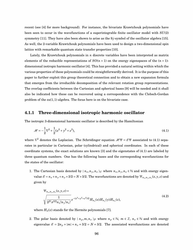
recent (see [4] for more background). For instance, the bivariate Krawtchouk polynomials have
been seen to occur in the wavefunctions of a superintegrable finite oscillator model with SU(2)
symmetry [11]. They have also been shown to arise as the 9 j-symbol of the oscillator algebra [15].
As well, the 2-variable Krawtchouk polynomials have been used to design a two-dimensional spin
lattice with remarkable quantum state transfer properties [10].
Lately, the Krawtchouk polynomials in n discrete variables have been interpreted as matrix
elements of the reducible representations of SO(n+1) on the energy eigenspaces of the (n+1)-
dimensional isotropic harmonic oscillator [4]. This has provided a natural setting within which the
various properties of these polynomials could be straightforwardly derived. It is the purpose of this
paper to further exploit this group theoretical connection and to obtain a new expansion formula
that emerges from the irreducible decomposition of the relevant rotation group representations.
The overlap coefficients between the Cartesian and spherical bases [9] will be needed and it shall
also be indicated how these can be recovered using a correspondence with the Clebsch-Gordan
problem of the su(1,1) algebra. The focus here is on the bivariate case.
4.1.1 Three-dimensional isotropic harmonic oscillator
The isotropic 3-dimensional harmonic oscillator is described by the Hamiltonian
H =−12∇2 + 1
2(x2 + y2 + z2), (4.1)
where ∇2 denotes the Laplacian. The Schrödinger equation HΨ = EΨ associated to (4.1) sepa-
rates in particular in Cartesian, polar (cylindrical) and spherical coordinates. In each of these
coordinate systems, the exact solutions are known [3] and the eigenstates of (4.1) are labeled by
three quantum numbers. One has the following bases and the corresponding wavefunctions for
the states of the oscillator:
1. The Cartesian basis denoted by | nx,ny,nz ⟩C where nx,ny,nz ∈ N and with energy eigen-
value E = nx+ny+ny+3/2= N+3/2. The wavefunctions are denoted by Ψnx,ny,nz (x, y, z) and
given by
Ψnx,ny,nz (x, y, z)=√1
2Nπ3/2nx!ny!nz!e−(x2+y2+z2)/2 Hnx (x)Hny(y)Hnz (z),
(4.2)
where Hn(x) stands for the Hermite polynomials [7].
2. The polar basis denoted by | nρ,m,nz ⟩P where nρ ∈ N, m ∈ Z, nz ∈ N and with energy
eigenvalue E = 2nρ + |m| + nz + 3/2 = N + 3/2. The associated wavefunctions are denoted
96

Ψnρ ,m,nz (ρ,φ, z) and given by
Ψnρ ,m,nz (ρ,φ, z)=(−1)nρ
π3/4
√nρ!
2nz nz!Γ(nρ+|m|+1)e−(ρ2+z2)/2ρ|m|L(|m|)
nρ(ρ2)Hnz (z)eimφ,
(4.3)
where L(α)n (x) are the Laguerre polynomials [7].
3. The spherical basis | nr,`,m ⟩S where nr ∈N, ` ∈N, m =−`, . . . ,` and with energy eigenvalue
E = 2nr +`+3/2= N +3/2. The wavefunctions are denoted Ψnr ,`,m(r,θ,φ) and given by
Ψnr ,`,m(r,θ,φ)=
(−1)nr e−r2/2 r`√
2nr!Γ(nr +`+3/2)
L(`+1/2)nr
(r2)Y m` (θ,φ),
(4.4)
where Y m`
(θ,φ) are the spherical harmonics [3].
It is directly seen that the energy level N has degeneracy (N+1)(N+2)/2. The creation/annihilation
operators
axi =1p2
(xi +∂xi ), a†xi= 1p
2(xi −∂xi ), i = 1,2,3,
with x1 = x, x2 = y, x3 = z obey the commutation relations
[axi ,a†x j
]= δi j, [axi ,ax j ]= 0, i, j = 1,2,3,
and have the following actions on the Cartesian basis states:
axi | nxi ⟩C =pnxi | nxi −1 ⟩C, a†
xi| nxi ⟩ =
√nxi +1 | nxi +1 ⟩C .
It follows that a†xi axi | nxi ⟩ = nxi | nxi ⟩C. In terms of these operators, (4.1) takes the form
H = a†xax +a†
yay +a†zaz +3/2, (4.5)
and one has indeed H | nx,ny,nz ⟩C = (N +3/2)| nx,ny,nz ⟩C.
4.1.2 SO(3)⊂ SU(3) and oscillator states
The Hamiltonian (4.5) of the 3-dimensional isotropic Harmonic oscillator is clearly invariant under
SU(3) transformations, which are generated by the constants of motion of the form a†i a j. For each
value of N, the Cartesian basis states | nx,ny,nz ⟩C support the completely symmetric irreducible
representation of SU(3). The Hamiltonian (4.1) is also manifestly invariant under SO(3)⊂ SU(3)
transformations. These rotations are generated by the three angular momentum generators
Lx =−i(a†yaz −a†
zay), L y =−i(a†zax −a†
xaz), Lz =−i(a†xay −a†
yax), (4.6)
97
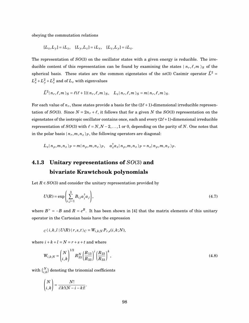
obeying the commutation relations
[Lx,L y]= iLz, [L y,Lz]= iLx, [Lz,L y]= iLx.
The representation of SO(3) on the oscillator states with a given energy is reducible. The irre-
ducible content of this representation can be found by examining the states | nr,`,m ⟩S of the
spherical basis. These states are the common eigenstates of the so(3) Casimir operator ~L2 =L2
x +L2y +L2
z and of Lz with eigenvalues
~L2| nr,`,m ⟩S = `(`+1)| nr,`,m ⟩S, Lz| nr,`,m ⟩S = m| nr,`,m ⟩S.
For each value of nr, these states provide a basis for the (2`+1)-dimensional irreducible represen-
tation of SO(3). Since N = 2nr +`, it follows that for a given N the SO(3) representation on the
eigenstates of the isotropic oscillator contains once, each and every (2`+1)-dimensional irreducible
representation of SO(3) with `= N, N −2, . . . ,1 or 0, depending on the parity of N. One notes that
in the polar basis | nr,m,nz ⟩P , the following operators are diagonal:
Lz| nρ,m,nz ⟩P = m| nρ,m,nz ⟩P , a†zaz| nρ,m,nz ⟩P = nz| nρ,m,nz ⟩P .
4.1.3 Unitary representations of SO(3) and
bivariate Krawtchouk polynomials
Let R ∈ SO(3) and consider the unitary representation provided by
U(R)= exp
(3∑
i, j=1Bi ja
†i a j
), (4.7)
where B> = −B and R = eB. It has been shown in [4] that the matrix elements of this unitary
operator in the Cartesian basis have the expression
C⟨ i,k, l |U(R) | r, s, t ⟩C =Wi,k;N Pr,s(i,k; N),
where i+k+ l = N = r+ s+ t and where
Wi,k;N =(
Ni,k
)1/2
RN33
(R13
R33
)i (R23
R33
)k, (4.8)
with( N
i,k)
denoting the trinomial coefficients(Ni,k
)= N!
i!k!(N − i−k)!.
98
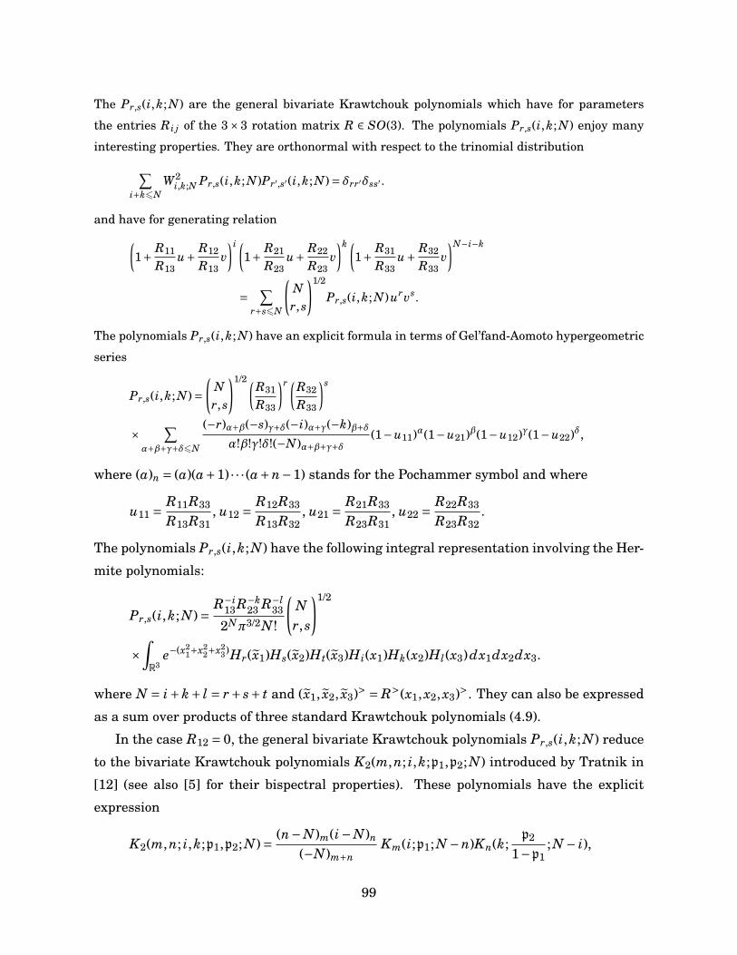
The Pr,s(i,k; N) are the general bivariate Krawtchouk polynomials which have for parameters
the entries Ri j of the 3×3 rotation matrix R ∈ SO(3). The polynomials Pr,s(i,k; N) enjoy many
interesting properties. They are orthonormal with respect to the trinomial distribution
∑i+k6N
W2i,k;N Pr,s(i,k; N)Pr′,s′(i,k; N)= δrr′δss′ .
and have for generating relation(1+ R11
R13u+ R12
R13v)i (
1+ R21
R23u+ R22
R23v)k (
1+ R31
R33u+ R32
R33v)N−i−k
= ∑r+s6N
(Nr, s
)1/2
Pr,s(i,k; N)urvs.
The polynomials Pr,s(i,k; N) have an explicit formula in terms of Gel’fand-Aomoto hypergeometric
series
Pr,s(i,k; N)=(
Nr, s
)1/2 (R31
R33
)r (R32
R33
)s
× ∑α+β+γ+δ6N
(−r)α+β(−s)γ+δ(−i)α+γ(−k)β+δα!β!γ!δ!(−N)α+β+γ+δ
(1−u11)α(1−u21)β(1−u12)γ(1−u22)δ,
where (a)n = (a)(a+1) · · · (a+n−1) stands for the Pochammer symbol and where
u11 = R11R33
R13R31, u12 = R12R33
R13R32, u21 = R21R33
R23R31, u22 = R22R33
R23R32.
The polynomials Pr,s(i,k; N) have the following integral representation involving the Her-
mite polynomials:
Pr,s(i,k; N)= R−i13R−k
23 R−l33
2Nπ3/2N!
(Nr, s
)1/2
×∫R3
e−(x21+x2
2+x23)Hr(x1)Hs(x2)Ht(x3)Hi(x1)Hk(x2)Hl(x3)dx1dx2dx3.
where N = i+k+ l = r+ s+ t and (x1, x2, x3)> = R>(x1, x2, x3)>. They can also be expressed
as a sum over products of three standard Krawtchouk polynomials (4.9).
In the case R12 = 0, the general bivariate Krawtchouk polynomials Pr,s(i,k; N) reduce
to the bivariate Krawtchouk polynomials K2(m,n; i,k;p1,p2; N) introduced by Tratnik in
[12] (see also [5] for their bispectral properties). These polynomials have the explicit
expression
K2(m,n; i,k;p1,p2; N)= (n−N)m(i−N)n
(−N)m+nKm(i;p1; N −n)Kn(k;
p2
1−p1; N − i),
99
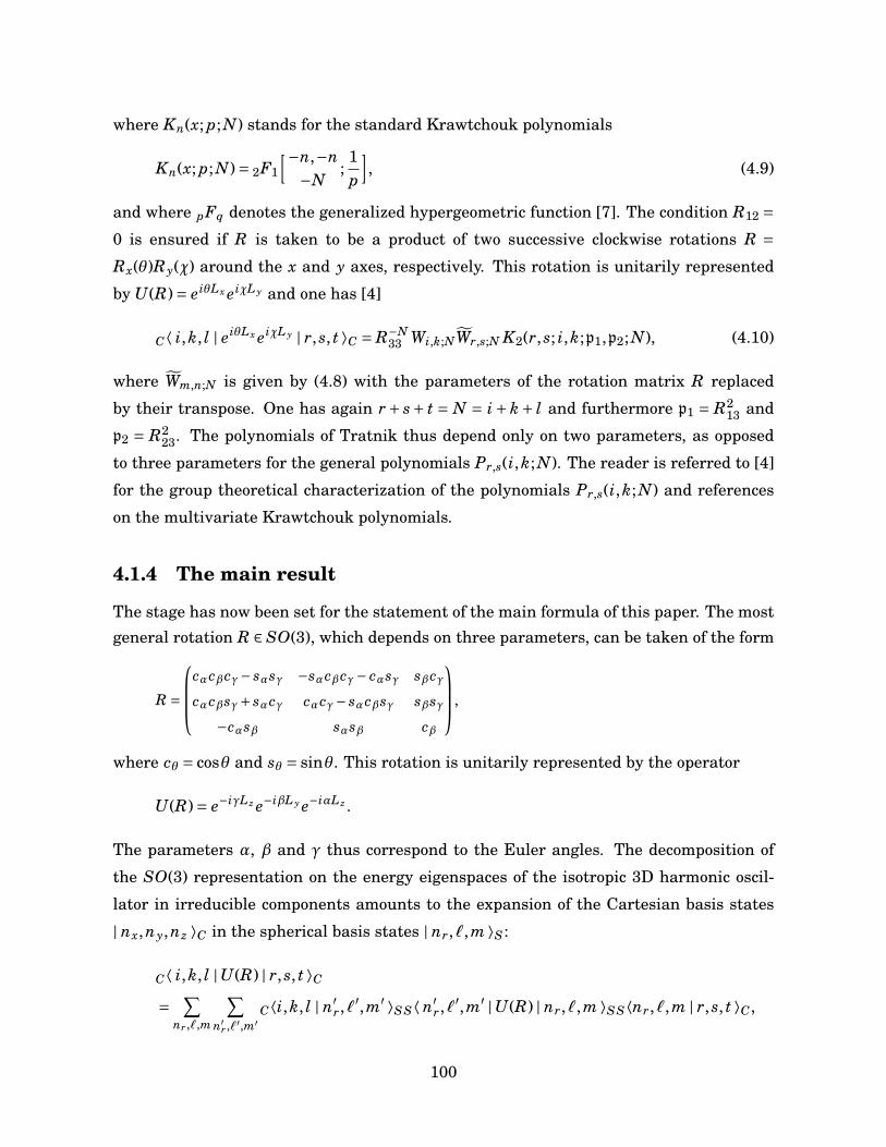
where Kn(x; p; N) stands for the standard Krawtchouk polynomials
Kn(x; p; N)= 2F1
[−n,−n−N
;1p
], (4.9)
and where pFq denotes the generalized hypergeometric function [7]. The condition R12 =0 is ensured if R is taken to be a product of two successive clockwise rotations R =Rx(θ)Ry(χ) around the x and y axes, respectively. This rotation is unitarily represented
by U(R)= eiθLx eiχL y and one has [4]
C⟨ i,k, l | eiθLx eiχL y | r, s, t ⟩C = R−N33 Wi,k;NWr,s;N K2(r, s; i,k;p1,p2; N), (4.10)
where Wm,n;N is given by (4.8) with the parameters of the rotation matrix R replaced
by their transpose. One has again r+ s+ t = N = i+ k+ l and furthermore p1 = R213 and
p2 = R223. The polynomials of Tratnik thus depend only on two parameters, as opposed
to three parameters for the general polynomials Pr,s(i,k; N). The reader is referred to [4]
for the group theoretical characterization of the polynomials Pr,s(i,k; N) and references
on the multivariate Krawtchouk polynomials.
4.1.4 The main result
The stage has now been set for the statement of the main formula of this paper. The mostgeneral rotation R ∈ SO(3), which depends on three parameters, can be taken of the form
R =
cαcβcγ− sαsγ −sαcβcγ− cαsγ sβcγcαcβsγ+ sαcγ cαcγ− sαcβsγ sβsγ
−cαsβ sαsβ cβ
,
where cθ = cosθ and sθ = sinθ. This rotation is unitarily represented by the operator
U(R)= e−iγLz e−iβL y e−iαLz .
The parameters α, β and γ thus correspond to the Euler angles. The decomposition of
the SO(3) representation on the energy eigenspaces of the isotropic 3D harmonic oscil-
lator in irreducible components amounts to the expansion of the Cartesian basis states
| nx,ny,nz ⟩C in the spherical basis states | nr,`,m ⟩S:
C⟨ i,k, l |U(R) | r, s, t ⟩C
= ∑nr ,`,m
∑n′
r ,`′,m′C⟨i,k, l | n′
r,`′,m′ ⟩SS⟨ n′r,`′,m′ |U(R) | nr,`,m ⟩SS⟨nr,`,m | r, s, t ⟩C,
100

where i + k + l = N = r + s+ t. The following expression for the bivariate Krawtchouk
polynomials Pr,s(i,k; N) stems from this decomposition:
Pr,s(i,k; N)=W−1i,k;N
× ∑nr ,`
2nr+`=N
∑m,m′=−`
D(`)mm′(R) C⟨i,k, l | nr,`,m′ ⟩S S⟨nr,`,m | r, s, t ⟩C. (4.11)
The matrix elements D(`)m′m(R) = S⟨ n′
r,`′,m′ | U(R) | nr,`,m ⟩S of the so(3) Wigner D-
matrix are given by [8]
D(`)m′m = δnrn′
rδ``′ e−i(γm′+αm)
× (−1)m′+` sin2` (β2
)tanm+m′ (β
2)[(
2`m+`
)(2`
m′+`
)]1/2
Km+`(m′+`; sin2 β
2; 2`
).
The overlap coefficients between the Cartesian and spherical bases are obtained by using
the intermediary decomposition over the polar basis states and read
S⟨nr,`,m | r, s, t ⟩C =∑nρ
(−1)nr+nρ (−i)m+|m|(−σm i)sp
2C
1/2+qr2 , 1/2+qs
2 , 1+|m|2
r,s,nρC
1+|m|2 , 1/2+qt
2 , `+3/22
nρ ,t,nr,
(4.12)
where 2nρ + |m| = r+ s, 2nr +` = r+ s+ t and w = 2w+ qw with w = r, s, t and qw = 0,1.
In (4.12), the square root factor should be omitted for m = 0 and σm = 1 if m > 0 and −1
otherwise. The coefficients C are given by
Cν1,ν2,ν12n1,n2,n12 = δν12,ν1+ν2+x
[(2ν1)n1(2ν2)n2(2ν1)x
n1!n2!n12!x!(2ν2)x(2ν1 +2ν2 +2x)n12(2ν1 +2ν2 + x−1)x
]1/2
× (x+n12)! Rn1(λ(x);2ν1 −1,2ν2 −1;n1 +n2),
with x = n1+n2−n12, where Rn(λ(x);γ,δ; N) are the dual Hahn polynomials [7] (see (4.28)).
One has S⟨nr,`,m | r, s, t ⟩C = C⟨r, s, t | nr,`,m ⟩∗S, where x∗ denotes the complex conjugate
of x. Note that in (4.11), the dependence of the polynomials Pr,s(i,k; N) on the parameters
is all contained in the Wigner function.The main formula (4.11) can also be used for the special case R12 = 0 corresponding
to the Tratnik polynomials. Indeed, since one has eiθLx eiχL y = e−i π2 L y eiθLz eiχL y ei π2 L y , itfollows that
C⟨ i,k, l | eiθLx eiχL y | r, s, t ⟩C = (−1)l+tC⟨ l,k, i | eiθLz eiχL y | t, s, r ⟩C, (4.13)
101
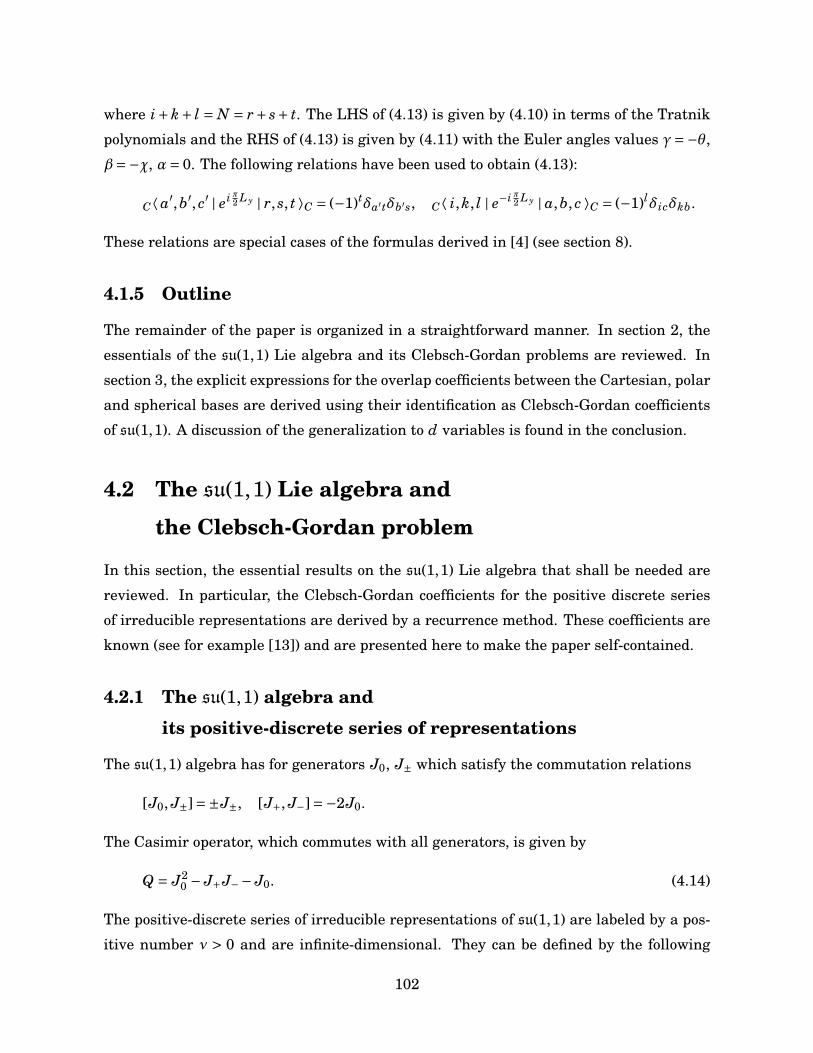
where i+ k+ l = N = r+ s+ t. The LHS of (4.13) is given by (4.10) in terms of the Tratnik
polynomials and the RHS of (4.13) is given by (4.11) with the Euler angles values γ=−θ,
β=−χ, α= 0. The following relations have been used to obtain (4.13):
C⟨ a′,b′, c′ | ei π2 L y | r, s, t ⟩C = (−1)tδa′tδb′s, C⟨ i,k, l | e−i π2 L y | a,b, c ⟩C = (−1)lδicδkb.
These relations are special cases of the formulas derived in [4] (see section 8).
4.1.5 Outline
The remainder of the paper is organized in a straightforward manner. In section 2, the
essentials of the su(1,1) Lie algebra and its Clebsch-Gordan problems are reviewed. In
section 3, the explicit expressions for the overlap coefficients between the Cartesian, polar
and spherical bases are derived using their identification as Clebsch-Gordan coefficients
of su(1,1). A discussion of the generalization to d variables is found in the conclusion.
4.2 The su(1,1) Lie algebra and
the Clebsch-Gordan problem
In this section, the essential results on the su(1,1) Lie algebra that shall be needed are
reviewed. In particular, the Clebsch-Gordan coefficients for the positive discrete series
of irreducible representations are derived by a recurrence method. These coefficients are
known (see for example [13]) and are presented here to make the paper self-contained.
4.2.1 The su(1,1) algebra and
its positive-discrete series of representations
The su(1,1) algebra has for generators J0, J± which satisfy the commutation relations
[J0, J±]=±J±, [J+, J−]=−2J0.
The Casimir operator, which commutes with all generators, is given by
Q = J20 − J+J−− J0. (4.14)
The positive-discrete series of irreducible representations of su(1,1) are labeled by a pos-
itive number ν > 0 and are infinite-dimensional. They can be defined by the following
102
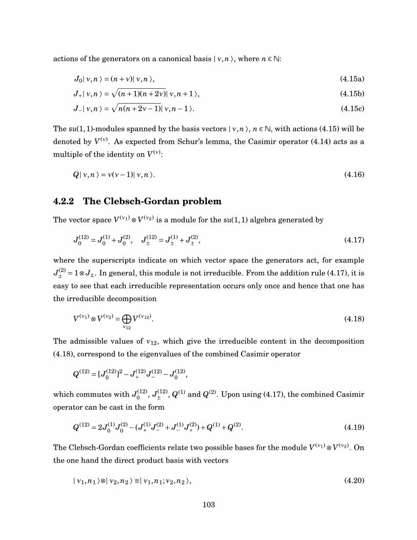
actions of the generators on a canonical basis | ν,n ⟩, where n ∈N:
J0| ν,n ⟩ = (n+ν)| ν,n ⟩, (4.15a)
J+| ν,n ⟩ =√
(n+1)(n+2ν)| ν,n+1 ⟩, (4.15b)
J−| ν,n ⟩ =√
n(n+2ν−1)| ν,n−1 ⟩. (4.15c)
The su(1,1)-modules spanned by the basis vectors | ν,n ⟩, n ∈N, with actions (4.15) will be
denoted by V (ν). As expected from Schur’s lemma, the Casimir operator (4.14) acts as a
multiple of the identity on V (ν):
Q| ν,n ⟩ = ν(ν−1)| ν,n ⟩. (4.16)
4.2.2 The Clebsch-Gordan problem
The vector space V (ν1) ⊗V (ν2) is a module for the su(1,1) algebra generated by
J(12)0 = J(1)
0 + J(2)0 , J(12)
± = J(1)± + J(2)
± , (4.17)
where the superscripts indicate on which vector space the generators act, for example
J(2)± = 1⊗J±. In general, this module is not irreducible. From the addition rule (4.17), it is
easy to see that each irreducible representation occurs only once and hence that one has
the irreducible decomposition
V (ν1) ⊗V (ν2) =⊕ν12
V (ν12). (4.18)
The admissible values of ν12, which give the irreducible content in the decomposition
(4.18), correspond to the eigenvalues of the combined Casimir operator
Q(12) = [J(12)0 ]2 − J(12)
+ J(12)− − J(12)
0 ,
which commutes with J(12)0 , J(12)
± , Q(1) and Q(2). Upon using (4.17), the combined Casimir
operator can be cast in the form
Q(12) = 2J(1)0 J(2)
0 − (J(1)+ J(2)
− + J(1)− J(2)
+ )+Q(1) +Q(2). (4.19)
The Clebsch-Gordan coefficients relate two possible bases for the module V (ν1)⊗V (ν2). On
the one hand the direct product basis with vectors
| ν1,n1 ⟩⊗| ν2,n2 ⟩ ≡| ν1,n1;ν2,n2 ⟩, (4.20)
103
and on the other hand, the “coupled” basis with vectors | ν12,n12 ⟩ defined by
Q(12)| ν12,n12 ⟩ = ν12(ν12 −1)| ν12,n12 ⟩, J(12)0 | ν12,n12 ⟩ = (n12 +ν12)| ν12,n12 ⟩.
(4.21)
In both bases, the Casimir operators Q(1), Q(2) act as multiples of the identity. The two
bases are orthonormal and span the representation space V (ν1) ⊗V (ν2). Hence it follows
that they are related by a unitary transformation
| ν12,n12 ⟩ =∑
n1,n2
Cν1,ν2,ν12n1,n2,n12 | ν1,n1;ν2,n2 ⟩. (4.22)
By virtue of (4.17) and (4.21), it is clear that the condition
n12 +ν12 = n1 +n2 +ν1 +ν2,
holds in the decomposition (4.22). Since n12 is an integer, it follows that
ν12 = ν1 +ν2 + x, n12 + x = n1 +n2, (4.23)
where x ∈ 0, . . . , N for a given value of N = n1 +n2. The coefficients Cν1,ν2,ν12n1,n2,n12 , which can
be written
Cν1,ν2,ν12n1,n2,n12 = ⟨ ν1,n1;ν2,n2 | ν12,n12 ⟩, (4.24)
are the Clebsch-Gordan coefficients for the positive-discrete series of irreducible repre-
sentations su(1,1).
4.2.3 Explicit expression for the Clebsch-Gordan coefficients
The explicit expression for the Clebsch-Gordan coefficients (4.24) is known [13], hence
only a short derivation using a recurrence relation is presented. By definition of the
coupled basis states (4.21), one has
ν12(ν12 −1)C ν1,ν2,ν12n1,n2,n12 = ⟨ ν1,n1;ν2,n2 |Q(12) | ν12,n12 ⟩. (4.25)
On the other hand, upon using (4.19) and the actions (4.15), one finds
⟨ ν1,n1;ν2,n2 |Q(12) | ν12,n12 ⟩ = 2(n1 +ν1)(n2 +ν2) Cν1,ν2,ν12n1,n2,n12
−√
n1(n1 +2ν1 −1)(n2 +1)(n2 +2ν2)C ν1,ν2,ν12n1−1,n2+1,n12
+ν1(ν1 −1)C ν1,ν2,ν12n1,n2,n12
−√
n2(n2 +2ν2 −1)(n1 +1)(n1 +2ν1)C ν1,ν2,ν12n1+1,n2−1,n12
+ν2(ν2 −1)C ν1,ν2,ν12n1,n2,n12 . (4.26)
104
For a given value of N = n1+n2, taking n1 = n and n2 = N −n, one can use the conditions
(4.23) to make explicit the dependence of C on x:
Cν1,ν2,ν12n1,n2,n12 =ωPn(x;ν1,ν2; N),
where ω = Cν1,ν2,ν1+ν2+x0,N,N−x and P0(x) = 1. With these definitions, it follows from (4.25) and
(4.26) that Pn(x) satisfies the three-term recurrence relation
λ(x)Pn(x;ν1,ν2; N)= 2n(N −n)+ν2n+ν1(N −n)Pn(x;ν1,ν2; N)
+Wn Pn−1(x;ν1,ν2; N)+Wn+1 Pn+1(x;ν1,ν2; N).
where
λ(x)= x(x+2ν1 +2ν2 −1)
and where
Wn =−[n(N −n+1)(n+2ν1 −1)(N −n+2ν2)]1/2.
Upon taking Pn(x;ν1,ν2; N)= [W1 . . .Wn]−1Pn(x;ν1,ν2; N), one finds
λ(x)Pn(x)= Pn+1(x)− (An +Cn)Pn(x)+ An−1CnPn−1(x), (4.27)
where
An = (n−N)(n+2ν1), Cn = n(n−2ν2 −N).
It is directly seen from (4.27) that the polynomials Pn(x) correspond to the monic dual
Hahn polynomials Rn(λ(x);γ,δ; N) with parameters γ= 2ν1 −1 and δ= 2ν2 −1. The dual
Hahn polynomials are defined by [7]
Rn(λ(x);γ,δ; N)= 3F2
[−n,−x, x+γ+δ+1γ+1,−N
;1]. (4.28)
Since the orthonormality condition∑ν12,n12
ν12+n12=n1+n2+ν1+ν2
Cν1,ν2,ν12n1,n2,n12C
ν1,ν2,ν12n′
1,n′2,n12
= δn1n′1δn2n′
2,
must hold, one can use the orthogonality relation of the dual Hahn polynomials to com-
pletely determine the coefficients Cν1,ν2,ν12n1,n2,n12 up to a phase factor. One finds
Cν1,ν2,ν12n1,n2,n12 =
[(2ν1)n1(2ν2)n2(2ν1)x
n1!n2!n12!x!(2ν2)x(2ν1 +2ν2 +2x)n12(2ν1 +2ν2 + x−1)x
]1/2
× (x+n12)! Rn1(λ(x);2ν1 −1,2ν2 −1;n1 +n2), (4.29)
105
which is valid provided that the conditions (4.23) hold. Note that one also has
∑n1,n2
Cν1,ν2,ν12n1,n2,n12C
ν1,ν2,ν′12n1,n2,n′
12= δn12n′
12δν12ν
′12
,
where the sum is restricted by n1 +n2 = n12 +ν12 −ν1 −ν2.
4.3 Overlap coefficients for the isotropic 3D harmonic
oscillator
In this section, the explicit expressions for the overlap coefficients between the Cartesian,
polar and spherical bases for the states of the isotropic 3D harmonic oscillator are given.
Again, these expressions are not new and can be found in [9]. Since these results are not
so readily accessible however, we rederive them here using an interpretation in terms of
the Clebsch-Gordan coefficients given in (4.29).
4.3.1 The Cartesian/polar overlaps
The overlap coefficients between the Cartesian | nx,ny,nz ⟩C and polar | nρ,m,n′z ⟩P basis
states of the oscillator are defined by
C⟨nx,ny,nz | nρ,m,n′z ⟩P .
It is obvious that
C⟨nx,ny,nz | nρ,m,n′z ⟩P = δnz,n′
z C⟨nx,ny,nz | nρ,m,nz ⟩P .
One has the expansion
| nρ,m,nz ⟩P = ∑nx,ny
C⟨nx,ny,nz | nρ,m,nz ⟩P | nx,ny,nz ⟩C, (4.30)
where the condition nx + ny = 2nρ + |m| holds since only the states in the same energy
eigenspace can be related to one another. The states | nx,ny ⟩C =| nx ⟩⊗| ny ⟩ can be
identified with vectors | ν1,n1;ν2,n2 ⟩ of the direct product basis for a su(1,1)-module
V (νx) ⊗V (νy). Indeed, it is directly checked that the operators
J(xi)0 = 1
2(a†
xiaxi +1/2), J(xi)+ = 1
2(a†
xi)2, J(xi)− = 1
2a2
xi, (4.31)
106
with i = 1,2, realize the su(1,1) algebra and that the Cartesian states | nxi ⟩, with the
quantum number nxi either even or odd, are basis vectors for an irreducible module V (νxi )
with representation parameters νxi = 1/4 if nxi is even and νxi = 3/4 if nxi is odd. Hence
we have the identification
| 2nx + qx,2ny + qy ⟩C ∼| 1/4+ qx/2, nx;1/4+ qy/2, ny ⟩ ≡| ν1,n1;ν2,n2 ⟩, (4.32)
where qx, qy ∈ 0,1 and where the third quantum number nz as been suppressed from
the Cartesian states in (4.32) to facilitate the correspondence with the notation used in
the previous section.
The polar basis states | nρ,m,nz ⟩P can be identified with vectors of the “coupled” basis.
Indeed, consider the realization of the su(1,1) algebra obtained by taking
J(xy)0 = J(x)
0 + J(y)0 , J(xy)
± = J(x)± + J(y)
± .
By definition, the states | nρ,m,nz ⟩P satisfy
Lz| nρ,m,nz ⟩P = m| nρ,m,nz ⟩P .
Furthermore, a direct computation shows that the coupled Casimir Q(xy) operator can be
expressed in terms of Lz in the following way:
Q(xy) = 14
(L2z −1).
Hence it follows that the polar basis states are eigenvectors of the combined Casimir
operator Q(xy) with eigenvalue
Q(xy)| nρ,m ⟩P = 14
(m2 −1)| nρ,m ⟩P . (4.33)
Since from (4.30), (4.31) and nx +ny = 2nρ+|m| one also has
J(xy)0 | nρ,m,nz ⟩P =
(nρ+ |m|
2+1/2
)| nρ,m,nz ⟩P ,
it is seen that the polar basis states | nρ,m,nz ⟩P correspond to coupled su(1,1) basis states
of V (νxy) with representation parameter νxy = (|m|+1)/2. One thus writes
| nρ,m,nz ⟩P ∼| 1+|m|2
,nρ ⟩ ≡| ν12,n12 ⟩. (4.34)
The correspondence (4.32), (4.34) can now be used to recover the overlap coefficients be-
tween the Cartesian and polar bases of the 3D isotropic harmonic oscillator. One needs to
107

keep in mind that for m 6= 0, there is a sign ambiguity in (4.34) which has to be taken into
account to ensure the orthonormality conditions for the overlap coefficients. One finds
C⟨nx,ny,nz | nρ,0,n′z ⟩P = eiφδnz,n′
zCν1,ν2,ν12n1,n2,n12 ,
for m = 0
C⟨nx,ny,nz | nρ,m,n′z ⟩P = eiφ
p2δnz,n′
zCν1,ν2,ν12n1,n2,n12 ,
for m 6= 0, where eiφ is a phase factor that remains to be evaluated. The correspondence
between the quantum numbers and representation parameters is given by
ν1 = 1/4+ qx/2, ν2 = 1/4+ qy/2, ν12 = (1+|m|)/2, (4.35a)
n1 = nx, n2 = ny, n12 = nρ, (4.35b)
where nxi = 2nx + qx with qxi ∈ 0,1. The remaining phase factor can be evaluated by
requiring that the expansion
Ψnρ ,m,n′z(ρ,φ, z)= ∑
nx,nyC⟨nx,ny,nz | nρ,m,n′
z ⟩P Ψnx,ny,nz (x, y, z),
holds for the wavefunctions. By inspection of (4.2) and (4.3), one finds
eiφ = (−1)nx+nρ (σm i)ny , with σm =
1 m> 0,
−1 m < 0.
The complete expression for the overlaps is therefore given by
C⟨nx,ny,nz | nρ,m,n′z ⟩P = δnzn′
z
((−1)nx+nρ (σm i)ny
p2
)Cν1,ν2,ν12n1,n2,n12 , (4.36)
with the identification (4.35) and where it is understood that thep
2 factor is to be omitted
when m = 0.
4.3.2 The polar/spherical overlaps
The overlap coefficients between the polar and spherical bases are defined by
P⟨nρ,m′,nz | nr,`,m ⟩S.
Since both set of basis states are eigenstates of Lz, it follows that one can write
P⟨nρ,m′,nz | nr,`,m ⟩S = δmm′ P⟨nρ,m,nz | nr,`,m ⟩S.
108
One has the decomposition
| nr,`,m ⟩S = ∑nρ ,nz
P⟨nρ,m,nz | nr,`,m ⟩S | nρ,m,nz ⟩P , (4.37)
where the condition 2nρ + |m| + nz = 2nr + ` holds since only the states with identical
energies can be related to one another. The states | nρ,m ⟩ and | nz ⟩ have already been
identified with basis vectors of irreducible su(1,1) representations. We thus write the
polar basis states | nρ,m,nz ⟩P =| nρ,m ⟩⊗| nz ⟩ as direct product vectors
| nρ,m,2nz + qz ⟩P ∼| (1+|m|)/2,nρ;1/4+ qz/2, nz ⟩ ≡| ν1,n1;ν2,n2 ⟩.
The spherical basis states | nr,`,m ⟩S can be identified with those of the “coupled” basis.
Indeed, consider the su(1,1) algebra obtained by taking
J((xy)z)0 = J(xy)
0 + J(z)0 , J((xy)z)
± = J(xy)± + J(z)
± . (4.38)
By definition, the states | nr,`,m ⟩S satisfy
~L2| nr,`,m ⟩S = `(`+1)| nr,`,m ⟩S,
where~L2 = L2x+L2
y+L2z. Furthermore, a direct computation shows that~L2 and the coupled
Casimir operator Q((xy)z) are related by
Q((xy)z) = 14
(~L2 − 3
4
).
Hence one may write
Q((xy)z)| nr,`,m ⟩S = (`/2+3/4)(`/2−1/4)| nr,`,m ⟩S.
Since from (4.37), (4.38) and the condition 2nr +`= 2nρ+|m|+nz one has
J((xy)z)0 | nr,`,m ⟩S = nr + (`+3)/2| nr,`,m ⟩S,
it follows that the states of the spherical basis correspond to coupled su(1,1) states
| nr,`,m ⟩S ∼| `+3/22
,nr ⟩ ∼| ν12,n12 ⟩.
Using this identification, one writes
P⟨nρ,m,nz | nr,`,m ⟩S = eiψδmm′ C ν1,ν2,ν12n1,n2,n12 ,
109
where
ν1 = 1+|m|2
, ν2 = 1/2+ qz
2, ν12 = `+3/2
2, (4.39a)
n1 = nρ, n2 = nz, n12 = nr, (4.39b)
and with nz = 2nz + qz. The phase factor eiψ can be determined by requiring that the
expansion formula
Ψnr ,`,m(ρ,θ,φ)= ∑nρ ,nz
P⟨nρ,m,nz | nr,`,m ⟩S Ψnρ ,m,nz (ρ,φ, z),
holds for the wavefunctions. Upon inspecting (4.3) and (4.4), one finds that eiψ = im+|m|.
Hence the following expression holds
P⟨nρ,m,nz | nr,`,m′ ⟩S = δmm′ im+|m|C ν1,ν2,ν12n1,n2,n12 , (4.40)
with the identification (4.39). Note that one has also
S⟨nr,`,m′ | nρ,m,nz ⟩P = δmm′ (−i)m+|m|C ν1,ν2,ν12n1,n2,n12 ,
since the Clebsch-Gordan coefficients Cν1,ν2,ν12n1,n2,n12 are real.
4.4 Conclusion
To sum up, we have obtained a new explicit formula for the bivariate Krawtchouk poly-
nomials in terms of the standard (univariate) Krawtchouk and dual Hahn polynomials.
Furthermore, the explicit expressions for the overlap coefficients of the isotropic oscillator
have been rederived using a correspondence with the Clebsch-Gordan problem of su(1,1).
In [4], the results obtained using SO(3) were seen to extend directly to higher dimen-
sions and indeed the d-variable Krawtchouk polynomials can be interpreted as matrix
elements of unitary reducible SO(d+1) representations on (Cartesian) oscillator states.
The main result (4.11) obtained here for the bivariate Krawtchouk polynomials can also
be generalized to d variables. The derivation is similar in spirit to the one presented here
but is quite technical. We now outline how this generalization proceeds.
Let R ∈ SO(d+1). The matrix elements of the reducible SO(d+1) unitary represen-
tation (4.7) in the Cartesian basis of the E = N + d/2 energy eigenspace of the (d + 1)-
dimensional isotropic harmonic oscillator are expressed as follows [4]:
⟨ i1, . . . , id+1 |U(R) | n1, . . . ,nd+1 ⟩ =Wi1,...,id ;N Pn1,...,nd (i1, . . . , id; N),
110
where Pn1,...,nd (i1, . . . , id; N) are the multivariate Krawtchouk polynomials and where
Wi1,...,id ;N =(
Ni1, . . . , id
)1/2
R i11,d+1 . . .R id
d,d+1RN−i1−...−idd+1,d+1 ,
with∑d+1
k=1 ik = ∑d+1k=1 nk = N. The decomposition of this SO(d + 1) representation in ir-
reducible components can be accomplished by a passage to a canonical basis which cor-
responds to the separation of variables of the Schrödinger equation in hyperspherical
coordinates [2]. These basis states are denoted by | nr,λ,µ1, . . .µd−1 ⟩ with nr,∈ N and
λ>µ1 > · · ·> |µd−1|> 0. They are eigenstates of the (d+1)-dimensional harmonic oscilla-
tor Hamiltonian with energy E = 2nr+λ+d/2 and the corresponding wavefunctions can be
expressed in terms of Laguerre polynomials and hyperspherical harmonics [1, 14]. These
states form a basis for (class 1) irreducible representations of SO(d +1) [13]. They are
eigenvectors of the quadratic Casimir operator of SO(d+1) with eigenvalue λ(λ+d−1)
and of the quadratic Casimir operators of each element in the canonical subgroup chain
SO(d+1) ⊃ SO(d) ⊃ ·· · ⊃ SO(2) with eigenvalues µ1(µ1 +d−2),µ2(µ2 +d−3) . . . ,µ2d−1 [2].
This is the origin of the parameters µi, i = 1, . . . ,d−1. For a given N, the SO(d+1) rep-
resentation on the eigenstates of the (d + 1)-dimensional oscillator contains once, each
and every (class one) irreducible representation of SO(d + 1) with λ = N, N − 2, . . . ,0,1
depending on the parity. This decomposition is equivalent to the decomposition of the
quasi-regular representation of SO(d+1) [13]. Upon introducing the states correspond-
ing to separation in hyperspherical coordinates, one is led to the decomposition formula
Pn1,...,nd (i1, . . . , id; N)=W−1i1,...,id ;N
× ∑nr ,λ
∑µ,µ′
⟨ nr,λ,µ′1, . . . ,µ′
d−1 |U(R) | nr,λ,µ1, . . . ,µd−1 ⟩
×⟨ i1, . . . , id+1 | nr,λ,µ′1, . . . ,µ′
d−1 ⟩⟨ nr,λ,µ1, . . . ,µd−1 | n1, . . . ,nd+1 ⟩,
where 2nr +λ = N = i1 + ·· ·+ id+1 = n1 + ·· ·+ nd+1 and where µ denotes the multi-index
(µ1, . . . ,µd−1) with λ > µ1 > µ2 > · · · > |µd−1| > 0. The overlap coefficients can be eval-
uated as sums of products of d su(1,1) Clebsch-Gordan coefficients using successive re-
couplings of the quantum numbers, as was done in Section 3. The matrix elements
⟨ nr,λ,µ′1, . . . ,µ′
d−1 | U(R) | nr,λ,µ1, . . . ,µd−1 ⟩ are very involved. They can be evaluated
only recursively using the canonical subgroup chain of SO(d+1). See [13] for details.
111
References
[1] J. Avery. Hyperspherical Harmonics; Some Properties and Applications. In E. S. Kryachko
and J. L. Calais, editors, Conceptual Trends in Quantum Chemistry. Springer Netherlands,
1994.
[2] J. Avery. Harmonic polynomials, hyperspherical harmonics, and atomic spectra. J. Comp.
Appl. Math., 233:1366–1379, 2010.
[3] C. Cohen-Tannoudji, B. Diu, and F. Laloe. Quantum Mechanics. Wiley-VCH, 1st edition,
1991.
[4] V.X. Genest, L. Vinet, and A. Zhedanov. The multivariate Krawtchouk polynomials as matrix
elements of the rotation group representations on oscillator states. J. Phys. A: Math. Theor,
46:505203, 2013.
[5] J.S. Geronimo and P. Iliev. Bispectrality of multivariable Racah-Wilson polynomials. Constr.
Approx., 31:417–457, 2010.
[6] R.C. Griffiths. Orthogonal polynomials on the multinomial distribution. Australian Journal
of Statistics, 13:27–35, 1971.
[7] R. Koekoek, P.A. Lesky, and R.F. Swarttouw. Hypergeometric orthogonal polynomials and
their q-analogues. Springer, 1st edition, 2010.
[8] T. Koornwinder. Krawtchouk polynomials, a unification of two different group theoretic in-
terpretations. SIAM J. Math. Anal., 13:1011–1023, 1982.
[9] L.G.Mardoyan, G.S. Pogosyan, A.N. Sissakian, and V.M. Ter-Antonyan. Quantum systems
with hidden symmetry. Interbasis expansions (in Russian). Fizmatlit, 2006.
[10] H. Miki, S. Tsujimoto, L. Vinet, and A. Zhedanov. Quantum-state transfer in a two-
dimensional regular spin lattice of triangular shape. Phys. Rev. A, 85:062306, 2012.
[11] M. Miki, S. Post, L. Vinet, and A. Zhedanov. A superintegrable finite oscillator in two dimen-
sions with SU(2) symmetry. J. Phys. A: Math. Theor., 46:125207, 2013.
[12] M.V. Tratnik. Some multivariable orthogonal polynomials of the Askey tableau-discrete fam-
ilies. J. Math. Phys., 32:2337–2342, 1991.
[13] N.J. Vilenkin and A.U. Klimyk. Representations of Lie groups and Special Functions. Kluwer
Academic Publishers, 1991.
112

[14] Z. Wen and J. Avery. Some properties of hyperspherical harmonics. J.Math. Phys., 26:396,
1985.
[15] A. Zhedanov. 9 j-symbols of the oscillator algebra and Krawtchouk polynomials in two vari-
ables. J. Phys. A: Math. Theor., 30:8337–8357, 1997.
113

114
Chapitre 5
The multivariate Hahn polynomialsand the singular oscillator
V. X. Genest et L. Vinet (2014). The multivariate Hahn polynomials and the singular oscillator.
Journal of Physics A: Mathematical and Theoretical 47 455201
Abstract. Karlin and McGregor’s d-variable Hahn polynomials are shown to arise in the (d+1)-
dimensional singular oscillator model as the overlap coefficients between bases associated to the
separation of variables in Cartesian and hyperspherical coordinates. These polynomials in d dis-
crete variables depend on d +1 real parameters and are orthogonal with respect to the multidi-
mensional hypergeometric distribution. The focus is put on the d = 2 case for which the connection
with the three-dimensional singular oscillator is used to derive the main properties of the polyno-
mials: forward/backward shift operators, orthogonality relation, generating function, recurrence
relations, bispectrality (difference equations) and explicit expression in terms of the univariate
Hahn polynomials. The extension of these results to an arbitrary number of variables is presented
at the end of the paper.
5.1 Introduction
The objective of this article is to show that the multidimensional Hahn polynomials arise in the
quantum singular oscillator model as the overlap coefficients between energy eigenstate bases as-
sociated to the separation of variables in Cartesian and hyperspherical coordinates and to obtain
their properties from this framework. This offers an algebraic analysis of the multivariate Hahn
polynomials which is resting on their interpretation as overlap coefficients and on the special prop-
erties of the functions arising in the basis wavefunctions. For definiteness and ease of notation,
the emphasis shall be put on the case where the Hahn polynomials in two variables appear as
115
the Cartesian vs. spherical interbasis expansion coefficients for the three-dimensional singular
oscillator. It shall be indicated towards the end of the paper how these results can be extended
directly to an arbitrary number of variables.
The Hahn polynomials in one variable, which shall be denoted by hn(x;α,β; N), are the poly-
nomials of degree n in the variable x defined by [28, 30]
hn(x;α,β; N)= (α+1)n(−N)n 3F2
[−n,n+α+β+1,−xα+1,−N
;1],
where pFq is the generalized hypergeometric function [2] and where (a)n stands for the Pochham-
mer symbol (or shifted factorial)
(a)n = (a)(a+1) · · · (a+n−1), (a)0 ≡ 1.
These polynomials belong to the discrete part of the Askey scheme of hypergeometric orthogonal
polynomials [28]. They satisfy the orthogonality relation
N∑x=0
ρ(x;α,β; N)hn(x;α,β; N)hm(x;α,β; N)=λn(α,β; N) δnm,
with respect to the hypergeometric distribution [21]
ρ(x;α,β; N)=(Nx
)(α+1)x(β+1)N−x
(α+β+2)N, (5.1)
where(N
x)
are the binomial coefficients. The weight function (5.1) is positive provided that α,β>−1 or α,β<−N. The normalization factor λn reads
λn(α,β; N)= α+β+12n+α+β+1
N!n!(N −n)!
(α+1)n(β+1)n(N +α+β+2)n
(α+β+1)n. (5.2)
The polynomials hn(x;α,β; N) can be obtained from the generating function [28]
1F1
[ −xα+1
;−t]
1F1
[ x−Nβ+1
; t]=
N∑n=0
hn(x;α,β; N)(α+1)n(β+1)n
tn
n!, (5.3)
or from the dual generating function [24]
(−N)n n! (1+ t)N P(α,β)n
(1− t1+ t
)=
N∑x=0
(Nx
)hn(x;α,β; N) tx, (5.4)
where P(α,β)n (z) stands for the classical Jacobi polynomials [28]. In mathematical physics, the Hahn
polynomials are mostly known for their appearance in the Clebsch-Gordan coefficients of the su(2)
or su(1,1) algebras (see for example [36]). However, these polynomials have also been used in the
designing of spin chains allowing perfect quantum state transfer [1, 3, 37] and moreover, they
occur as exact solutions of certain discrete Markov processes [21].
116
The multivariable extension of the Hahn polynomials is due to Karlin and McGregor who ob-
tained these polynomials in [25] as exact solutions of a multidimensional genetics model. This
family of multidimensional polynomials is a member of the multivariate analogue of the dis-
crete Askey scheme proposed by Tratnik in [35] and generalized to the basic (q-deformed) case by
Gasper and Rahman in [9]. One of the key features of the polynomials in this multivariate scheme
is their bispectrality (in the sense of Duistermaat and Grünbaum [6]), which was established by
Geronimo and Iliev in [15] and by Iliev [19] in the q-deformed case. Since their introduction, the
multivariate Hahn polynomials have been studied from different points of view by a number of
authors [20, 31, 40, 38] and used in particular for applications in probability [18, 26]. Of partic-
ular relevance to the present article are the papers of Dunkl [7], Scarabotti [34] and Rosengren
[33], where the multivariate Hahn polynomials occur in an algebraic framework.
Here we give a physical interpretation of the multivariate Hahn polynomials by establishing
that they occur in the overlap coefficients between wavefunctions of the singular oscillator model
separated in Cartesian and hyperspherical coordinates. It will be seen that this framework pro-
vides a cogent foundation for the characterization of these polynomials: new derivations of known
formulas will be given and new identities will come to the fore. The results presented here are
in line with the physico-algebraic models that were exhibited in [13, 14], [11] and [10] where the
multivariate Krawtchouk, Meixner and Charlier polynomials were identified and characterized as
matrix elements of the representations of the rotation, Lorentz and Euclidean groups on oscillator
states. However the approach and techniques used in the present paper differ from the ones used
in [13], [11] and [10] as the multivariate Hahn polynomials do not arise as matrix elements of Lie
group representations.
The outline of the paper is the following. In section 2, the singular oscillator model in three-
dimensions is reviewed. The wavefunctions separated in Cartesian and spherical coordinates are
explicitly written and the corresponding constants of motion are given. In section 3, it is shown
that the expansion coefficients are expressed in terms of orthogonal polynomials in two discrete
variables that are orthogonal with respect to a two-variable generalization of the hypergeomet-
ric distribution. This is accomplished by bringing intertwining operators that raise/lower the
appropriate quantum numbers. In section 4, a generating function is derived by examining the
asymptotic behavior of the wavefunctions and this generating function is identified with the one
derived by Karlin and McGregor for the multivariate Hahn polynomials. Backward and forward
structure relations are obtained in section 5 and are seen to provide a factorization of the pair of
recurrence relations satisfied by the bivariate Hahn polynomials. In section 6, the two difference
equations are derived: one by factorization and the other by a direct computation involving one
of the symmetry operators responsible for the separation of variable in spherical coordinates. In
section 7, the explicit expression of the bivariate Hahn polynomials in terms of univariate Hahn
117
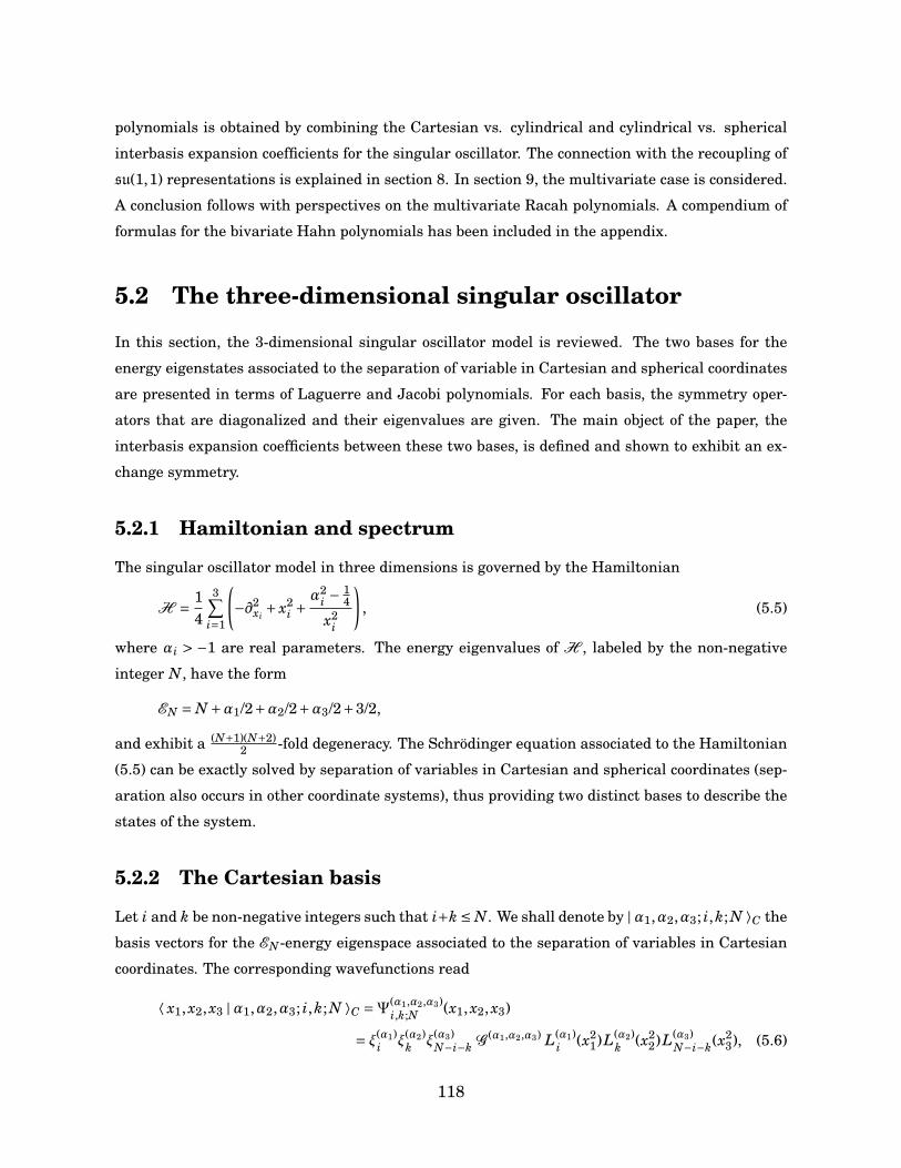
polynomials is obtained by combining the Cartesian vs. cylindrical and cylindrical vs. spherical
interbasis expansion coefficients for the singular oscillator. The connection with the recoupling of
su(1,1) representations is explained in section 8. In section 9, the multivariate case is considered.
A conclusion follows with perspectives on the multivariate Racah polynomials. A compendium of
formulas for the bivariate Hahn polynomials has been included in the appendix.
5.2 The three-dimensional singular oscillator
In this section, the 3-dimensional singular oscillator model is reviewed. The two bases for the
energy eigenstates associated to the separation of variable in Cartesian and spherical coordinates
are presented in terms of Laguerre and Jacobi polynomials. For each basis, the symmetry oper-
ators that are diagonalized and their eigenvalues are given. The main object of the paper, the
interbasis expansion coefficients between these two bases, is defined and shown to exhibit an ex-
change symmetry.
5.2.1 Hamiltonian and spectrum
The singular oscillator model in three dimensions is governed by the Hamiltonian
H = 14
3∑i=1
(−∂2
xi+ x2
i +α2
i − 14
x2i
), (5.5)
where αi > −1 are real parameters. The energy eigenvalues of H , labeled by the non-negative
integer N, have the form
EN = N +α1/2+α2/2+α3/2+3/2,
and exhibit a (N+1)(N+2)2 -fold degeneracy. The Schrödinger equation associated to the Hamiltonian
(5.5) can be exactly solved by separation of variables in Cartesian and spherical coordinates (sep-
aration also occurs in other coordinate systems), thus providing two distinct bases to describe the
states of the system.
5.2.2 The Cartesian basis
Let i and k be non-negative integers such that i+k ≤ N. We shall denote by |α1,α2,α3; i,k; N ⟩C the
basis vectors for the EN -energy eigenspace associated to the separation of variables in Cartesian
coordinates. The corresponding wavefunctions read
⟨ x1, x2, x3 |α1,α2,α3; i,k; N ⟩C =Ψ(α1,α2,α3)i,k;N (x1, x2, x3)
= ξ(α1)i ξ
(α2)k ξ
(α3)N−i−k G (α1,α2,α3) L(α1)
i (x21)L(α2)
k (x22)L(α3)
N−i−k(x23), (5.6)
118
where L(α)n (x) are the standard Laguerre polynomials [28] and where the gauge factor G (α1,α2,α3)
has the form
G (α1,α2,α3) = e−(x21+x2
2+x23)/2
3∏j=1
xα j+1/2j .
The normalization factors
ξ(α)n =
√2n!
Γ(n+α+1), (5.7)
where Γ(x) is the gamma function [2], ensure that the wavefunctions satisfy the orthogonality
relation
C⟨α1,α2,α3; i,k; N |α1,α2,α3; i′,k′; N ′ ⟩C =∫R3+
dx1dx2dx3
[Ψ
(α1,α2,α3)i,k;N
]∗Ψ
(α1,α2,α3)i′,k′;N ′ = δii′δkk′δNN ′ ,
where R+ stands for the non-negative real line and where z∗ stands for complex conjugation. The
Cartesian basis states are completely determined by the set of eigenvalue equations
K (1)0 |α1,α2,α3; i,k; N ⟩C = (i+α1/2+1/2)|α1,α2,α3; i,k; N ⟩C,
K (2)0 |α1,α2,α3; i,k; N ⟩C = (k+α2/2+1/2)|α1,α2,α3; i,k; N ⟩C,
H |α1,α2,α3; i,k; N ⟩C = EN |α1,α2,α3; i,k; N ⟩C,
where K (i)0 , i = 1,2, are the constants of motion ([H ,K (i)
0 ] = 0) associated to the separation of
variables in Cartesian coordinates. These (Hermitian) operators have the expression
K (i)0 = 1
4
(−∂2
xi+ x2
i +α2
i − 14
x2i
), (5.8)
and correspond to the one-dimensional singular oscillator Hamiltonian. For convenience, the
Cartesian basis states | α1,α2,α3; i,k; N ⟩C shall sometimes be written simply as | i,k; N ⟩C when
the explicit dependence on the parameters αi is not needed.
5.2.3 The spherical basis
Let m and n be non-negative integers such that m+n ≤ N. We shall denote by |α1,α2,α3;m,n; N ⟩S
the basis vectors for the EN -energy eigenspace associated to the separation of variables in spheri-
cal coordinates
x1 = rsinθ cosφ, x2 = rsinθsinφ, x3 = r cosθ.
119
In this case the corresponding wavefunctions are given by
⟨ r,θ,φ |α1,α2,α3;m,n; N ⟩S =Ξ(α1,α2,α3)m,n;N (r,θ,φ)
= η(α1,α2)m η
(2m+α12+1,α3)n ξ
(2m+2n+α123+2)N−m−n G (α1,α2,α3)
× P(α1,α2)m (−cos2φ) (sin2θ)mP(2m+α12+1,α3)
n (cos2θ) (r2)m+n L(2m+2n+α123+2)N−m−n (r2), (5.9)
where P(α,β)n (z) are the Jacobi polynomials and where we have introduced the notation
αi j =αi +α j, αi jk =αi +α j +αk.
The normalization factors
η(α,β)n =
√2(2n+α+β+1)n!Γ(n+α+β+1)
Γ(n+α+1)Γ(n+β+1), (5.10)
ensure that the wavefunctions Ξ(α1,α2,α3)m,n;N satisfy the orthogonality relation
S⟨α1,α2,α3;m,n; N |α1,α2,α3;m′,n′, N ′ ⟩S =∫ ∞
0
∫ π2
0
∫ π2
0r2 sinθdrdθdφ
[Ξ
(α1,α2,α3)m,n;N
]∗Ξ
(α1,α2,α3)m′,n′;N ′ = δmm′δnn′δNN ′ .
The spherical basis states |α1,α2,α3;m,n; N ⟩S are completely determined by the set of eigenvalue
equations
Q(12)|α1,α2,α3;m,n; N ⟩S =λ(12)m |α1,α2,α3;m,n; N ⟩S,
Q(123)|α1,α2,α3;m,n; N ⟩S =λ(123)m,n |α1,α2,α3;m,n; N ⟩S,
H |α1,α2,α3;m,n; N ⟩S = EN |α1,α2,α3;m,n; N ⟩S,
(5.11)
where the eigenvalues λ(12)m and λ(123)
m,n are given by
λ(12)m = (m+α12/2+1)(m+α12/2),
λ(123)m,n = (m+n+α123/2+3/2)(m+n+α123/2+1/2).
The (Hermitian) operators Q(12) and Q(123), which can be seen to commute with the Hamiltonian,
have the expressions
Q(12) = 14
−∂2
φ+α2
1 −1/4cos2φ
+ α22 −1/4
sin2φ−1
, (5.12a)
Q(123) = 14
−∂2
θ−ctgθ∂θ+α2
3 −1/4cos2θ
+ 1sin2θ
(−∂2
φ+α2
1 −1/4cos2φ
+ α22 −1/4
sin2φ
)− 3
4
. (5.12b)
120
In Cartesian coordinates, the spherical basis wavefunctions read
⟨ x1, x2, x3 |α1,α2,α3;m,n; N ⟩S =Ξ(α1,α2,α3)m,n;N (x1, x2, x3)
= η(α1,α2)m η
(2m+α12+1,α3)n ξ
(2m+2n+α123+2)N−m−n G (α1,α2,α3)(x2
1 + x22)mP (α1,α2)
m
(x2
2 − x21
x21 + x2
2
)
× (x21 + x2
2 + x23)nP (2m+α12+1,α3)
n
(x2
3 − x21 − x2
2
x21 + x2
2 + x23
)L(2m+2n+α123+2)
N−m−n (x21 + x2
2 + x23), (5.13)
and the operators Q(12), Q(123) have the form
Q(12) = 14
J2
3 + (x21 + x2
2)
(α2
1 −1/4
x21
+ α22 −1/4
x22
)−1
,
Q(123) = 14
J2
1 + J22 + J2
3 + (x21 + x2
2 + x23)
(α2
1 −1/4
x21
+ α22 −1/4
x22
+ α23 −1/4
x23
)− 3
4
,
(5.14)
where the J j are the familiar angular momentum operators
J1 = 1i(x2∂x3 − x3∂x2), J2 = 1
i(x3∂x1 − x1∂x3), J3 = 1
i(x1∂x2 − x2∂x1).
For notational convenience, the spherical basis vectors | α1,α2,α3;m,n; N ⟩S shall some-
times be written simply as | m,n; N ⟩S when the explicit dependence on the parameters
αi is not needed.
5.2.4 The main object
In this paper, we shall be concerned with the overlap coefficients between the Cartesian
and spherical bases. These coefficients are given by the integral
C⟨i,k; N | m,n; N ⟩S =∫R3+
dx1dx2dx3 [Ψ(α1,α2,α3)i,k;N (x1, x2, x3)]∗ Ξ(α1,α2,α3)
m,n;N (x1, x2, x3). (5.15)
Since the wavefunctions are real one has
C⟨i,k; N | m,n; N ⟩S = S⟨m,n; N | i,k; N ⟩C.
One can write the expansion formulas
| i,k; N ⟩C = ∑m,n
m+n≤N
S⟨m,n; N | i,k; N ⟩C | m,n; N ⟩S, (5.16a)
| m,n; N ⟩S = ∑i,k
i+k≤N
C⟨i,k; N | m,n; N ⟩S | i,k; N ⟩C, (5.16b)
121
relating the states of the Cartesian and spherical bases. Since these states are orthonor-
mal, the expansion coefficients satisfy the pair of orthogonality relations
∑i+k≤N
S⟨m,n; N | i,k; N ⟩CC⟨i,k; N | m′,n′; N ⟩S = δmm′δnn′ , (5.17a)∑m+n≤N
C⟨i,k; N | m,n; N ⟩SS⟨m,n; N | i′,k′; N ⟩C = δii′δkk′ . (5.17b)
Upon using the explicit expressions (5.6) and (5.13) of the wavefunctions in Cartesian co-
ordinates and the property P (α,β)n (−z)= (−1)nP (β,α)
n (z) satisfied by the Jacobi polynomials,
it is directly seen from (5.15) that the expansion coefficients obey the symmetry relation
C⟨α1,α2,α3; i,k; N |α1,α2,α3;m,n; N ⟩S
= (−1)mC⟨α2,α1,α3;k, i; N | α2,α1,α3;m,n; N ⟩S, (5.18)
which allows one to interchange the pairs (i,α1) and (k,α2). This symmetry shall prove
useful in what follows.
5.3 The expansion coefficients as orthogonal polyno-
mials in two variables
In this section, it is shown that the overlap coefficients between the Cartesian and spher-
ical basis states defined in the previous section are expressed in terms of orthogonal poly-
nomials in the two discrete variables i,k.
The expansion coefficients (5.15) can be cast in the form
C⟨α1,α2,α3; i,k; N |α1,α2,α3;m,n; N ⟩S =W (α1,α2,α3)i,k;N Q(α1,α2,α3)
m,n (i,k; N), (5.19)
where Q(α1,α2,α3)0,0 (i,k; N)≡ 1 and where we have defined
W (α1,α2,α3)i,k;N = C⟨α1,α2,α3; i,k; N |α1,α2,α3;0,0; N ⟩S.
5.3.1 Calculation of W (α1,α2,α3)i,k;N
The coefficient W (α1,α2,α3)i,k;N in (5.19) can be evaluated explicitly using the definition (5.15)
of the overlap coefficients. Indeed, upon taking m = n = 0 in (5.15) with the expressions
122
(5.6) and (5.13) for the wavefunctions, one finds
W (α1,α2,α3)i,k;N = ξ(α1)
i ξ(α2)k ξ
(α3)N−i−k η
(α1,α2)0 η
(α12+1,α3)0 ξ
(α123+2)N
∫ ∞
0
∫ ∞
0
∫ ∞
0dx1dx2dx3
e−(x21+x2
2+x23)
3∏j=1
(x2j )α j+1/2 L(α1)
i (x21)L(α2)
k (x22)L(α3)
N−i−k(x23)L(α123+2)
N (x21 + x2
2 + x23). (5.20)
Upon using twice the addition formula for the Laguerre polynomials [2]
L(α+β+1)n (x+ y)= ∑
`+k≤nL(α)`
(x)L(β)k (y),
one obtains the relation
L(α123+2)N (x2
1 + x22 + x2
3)= ∑i′+k′≤N
L(α1)i′ (x2
1)L(α2)k′ (x2
2)L(α3)N−i′−k′(x2
3).
The use of the above identity in (5.20) along with the orthogonality relation for the La-
guerre polynomials directly yields the explicit formula
W (α1,α2,α3)i,k;N = η
(α1,α2)0 η
(α12+1,α3)0 ξ
(α123+2)N
ξ(α1)i ξ
(α2)k ξ
(α3)N−i−k
.
With the help of the identity (a)n = Γ(a+n)Γ(a) for the Pochhammer symbol, the above expres-
sion is easily cast in the form
W (α1,α2,α3)i,k;N =
√N!
x!y!(N − x− y)!(α1 +1)i(α2 +1)k(α3 +1)N−i−k
(α1 +α2 +α3 +3)N. (5.21)
5.3.2 Raising relations
We shall now show that the functions Q(α1,α2,α3)m,n (i,k; N) appearing in (5.19) are polynomi-
als of degree m+n in the variable i,k by obtaining their raising relations.
Raising relation in m
Consider the operator C(α1,α2)+ having the following expression in spherical coordinates
C(α1,α2)+ = 1
2
[−∂φ+ tgφ (α1 +1/2)− (α2 +1/2)
tgφ
]. (5.22)
Using the structure relation (5.106) for the Jacobi polynomials, it can be directly checked
that one has
C(α1,α2)+ Ξ
(α1+1,α2+1,α3)m,n;N =
√(m+1)(m+α12 +2)Ξ(α1,α2,α3)
m+1,n;N+1. (5.23)
123
Consider the matrix element C⟨ α1,α2,α3; i,k; N | C(α1,α2)+ | α1 +1,α2 +1,α3;m,n; N −1 ⟩S.
On the one hand, the action (5.23) and the definition (5.19) give
C⟨α1,α2,α3; i,k; N | C(α1,α2)+ |α1 +1,α2 +1,α3;m,n; N −1 ⟩S
=√
(m+1)(m+α12 +2) W (α1,α2,α3)i,k;N Q(α1,α2,α3)
m+1,n (i,k; N). (5.24)
To obtain a raising relation, one needs to compute α1,α2,α3;i,k;N⟨ C |C(α1,α2)+ or equivalently
(recalling that the wavefunctions are real) (C(α1,α2)+ )†| α1,α2,α3; i,k; N ⟩C. This computa-
tion can be performed in a straightforward fashion by writing (5.22) in Cartesian coordi-
nates, acting on the wavefunctions (5.6) and using identities of the Laguerre polynomials
(see appendix of [12] for the details of a similar computation). One finds as a result
(C(α1,α2)+ )†Ψ
(α1,α2,α3)i,k;N
=√
i(k+α2 +1)Ψ(α1+1,α2+1,α3)i−1,k;N−1 −
√(i+α1 +1)kΨ(α1+1,α2+1,α3)
i,k−1;N−1 . (5.25)
Upon combining (5.24) and (5.25) and using (5.21), one arrives at the following contiguity
relation for the functions Q(α1,α2,α3)m,n (i,k; N):
c(α1,α2,α3)m,n;N Q(α1,α2,α3)
m+1,n (i,k; N)= i(k+α2 +1)Q(α1+1,α2+1,α3)m,n (i−1,k; N −1)
− k(i+α1 +1)Q(α1+1,α2+1,α3)m,n (i,k−1; N −1). (5.26)
where c(α1,α2,α3)m,n;N are the coefficients given by the expression
c(α1,α2,α3)m,n;N =
√N(α1+1)(α2+1)(N+α123+3)(m+1)(m+α12+2)
(α123+3)(α123+4) .
Raising relation in n
Consider the operator D(α1,α2,α3)+ defined as follows in spherical coordinates:
D(α1,α2,α3)+ =
Q(123) −Q(12) + α3 +1
2
[tgθ∂θ− α3 −1/2
cos2θ+ α3 +2
2
], (5.27)
where Q(12) and Q(123) are given by (5.12a) and (5.12b), respectively. Using the structure
relation (5.107) for the Jacobi polynomials as well as the eigenvalue equations (5.11), one
finds that the action of the operator D(α1,α2,α3)+ on the spherical basis states is
D(α1,α2,α3)+ Ξ
(α1,α2,α3+2)m,n;N =√(n+1)(n+α3 +2)(n+2m+α12 +2)(n+2m+α123 +3)Ξ(α1,α2,α3)
m,n+1;N+1 (5.28)
124
Consider the matrix element C⟨ α1,α2,α3; i,k; N | D(α1,α2,α3)+ | α1,α2,α3 +2;m,n; N −1 ⟩S.
Upon using the action (5.28) and the definition (5.15) of the overlap coefficients, one finds
on the one hand
C⟨α1,α2,α3; i,k; N | D(α1,α2,α3)+ |α1,α2,α3 +2;m,n; N −1 ⟩S =
√(n+1)(n+α3 +2)
×√
(n+2m+α12 +2)(n+2m+α123 +3)W (α1,α2,α3)i,k;N Q(α1,α2,α3)
m,n+1 (i,k; N) (5.29)
On the other hand, a direct computation shows that
(D(α1,α2,α3)+ )†Ψ
(α1,α2,α3)i,k;N =
√(i+1)(i+α1 +1)(N − i−k)(N − i−k−1)Ψ(α1,α2,α3+2)
i+1,k;N−1
+√
(k+1)(k+α2 +1)(N − i−k)(N − i−k−1)Ψ(α1,α2,α3+2)i,k+1;N−1
+√
i(i+α1)(N − i−k+α3 +1)(N − i−k+α3 +2)Ψ(α1,α2,α3+2)i−1,k;N−1
+√
k(k+α2)(N − i−k+α3 +1)(N − i−k+α3 +2)Ψ(α1,α2,α3+2)i,k−1;N−1
− (2i+2k+α12 +2)√
(N − i−k)(N − i−k+α3 +1)Ψ(α1,α2,α3+2)i,k;N−1 . (5.30)
Upon combining (5.29) and (5.30) and using (5.21), one obtains another contiguity relation
of the form
d(α1,α2,α3)m,n;N Q(α1,α2,α3)
m,n+1 (i,k; N)=(i+α1 +1)(N − i−k)(N − i−k−1)Q(α1,α2,α3+2)
m,n (i+1,k; N −1)
+ (k+α2 +1)(N − i−k)(N − i−k−1)Q(α1,α2,α3+2)m,n (i,k+1; N −1)
+ i(N − i−k+α3 +1)(N − i−k+α3 +2)Q(α1,α2,α3+2)m,n (i−1,k; N −1)
+k(N − i−k+α3 +1)(N − i−k+α3 +2)Q(α1,α2,α3+2)m,n (i,k−1; N −1)
− (N − i−k)(N − i−k+α3 +1)(2i+2k+α12 +2)Q(α1,α2,α3+2)m,n (i,k; N −1). (5.31)
where d(α1,α2,α3)m,n;N are the coefficients given by the expression
d(α1,α2,α3)m,n;N =
√N(N+α123+3)(α3+1)(α3+2)(n+1)(n+α3+2)(n+2m+α12+2)(n+2m+α123+3)
(α123+3)(α123+4) .
Since by definition Q(α1,α2,α3)0,0 (i,k; N)= 1, the relations (5.26) and (5.31) allow to construct
any Q(α1,α2,α3)m,n (i,k; N) iteratively. Writing up the first few cases, one observes that the
Q(α1,α2,α3)m,n (i,k; N) are polynomials of total degree m+n in the variables i,k.
5.3.3 Orthogonality relation
It is easy to see that the orthogonality relation (5.17a) satisfied by the transition coef-
ficients C⟨i,k; N | m,n; N ⟩S implies that the polynomials Q(α1,α2,α3)m,n (i,k; N) are orthogo-
125
nal. Indeed, upon inserting (5.19) in the relation (5.17a), one finds that the polynomials
Q(α1,α2,α3)m,n (i,k; N) are orthonormal∑
i+k≤Nw(α1,α2,α3)
i,k;N Q(α1,α2,α3)m,n (i,k; N)Q(α1,α2,α3)
m′,n′ (i,k; N)= δmm′δnn′ ,
with respect to the discrete weight function
w(α1,α2,α3)i,k;N =
[W (α1,α2,α3)
i,k;N
]2 =(
Ni,k
)(α1 +1)i(α2 +1)k(α3 +1)N−i−k
(α1 +α2 +α3 +3)N, (5.32)
where( Nx,y
)are the trinomial coefficients. It is clear that the weight (5.32) is a bivariate
extension of the Hahn weight function (5.1).
5.3.4 Lowering relations
It is also possible to obtain lowering relations for the polynomials Q(α1,α2,α3)m,n (i,k; N) using
the operators that are conjugate to C(α1,α2)+ and D(α1,α2,α3)
+ .
Lowering relation in m
Let us first examine the operator
C(α1,α2)− = 1
2
[∂φ+ tgφ (α1 +1/2)− (α2 +1/2)
tgφ
]. (5.33)
It is obvious from the definitions (5.22) and (5.33) that (C(α1,α2)± )† = C(α1,α2)
∓ . Furthermore,
it is directly verified with the help of (5.104) that (5.33) has the action
C(α1,α2)− Ξ
(α1,α2,α3)m,n;N =
√m(m+α12 +1)Ξ(α1+1,α2+1,α3)
m−1,n;N−1 . (5.34)
Consider the matrix element C⟨α1 +1,α2 +1,α3; i,k : N | C(α1,α2)− |α1,α2,α3;m,n; N +1 ⟩S.
Upon using (5.34) and the definition (5.19), one finds on the one hand
C⟨α1 +1,α2 +1,α3; i,k : N | C(α1,α2)− |α1,α2,α3;m,n; N +1 ⟩S
=√
m(m+α12 +1)W (α1+1,α2+1,α3)i,k;N Q(α1+1,α2+1,α3)
m−1,n (i,k; N). (5.35)
Upon writing (C(α1,α2)− )† in Cartesian coordinates and acting on the wavefunctions (5.6),
one finds on the other hand
(C(α1,α2)− )†Ψ
(α1+1,α2+1,α3)i,k;N =√
(i+1)(k+α2 +1)Ψ(α1,α2,α3)i+1,k;N+1 −
√(i+α1 +1)(k+1)Ψ(α1,α2,α3)
i,k+1;N+1. (5.36)
126
Combining (5.35) and (5.36) using (5.19) and (5.21), the following lowering relation for the
polynomials Q(α1,α2,α3)m,n (i,k; N) is obtained
e(α1,α2,α3)m,n;N Q(α1+1,α2+1,α3)
m−1,n (i,k; N)=Q(α1,α2,α3)
m,n (i+1,k; N +1)−Q(α1,α2,α3)m,n (i,k+1; N +1),
where
e(α1,α2,α3)m,n;N =
√m(m+α12+1)(α123+3)(α123+4)
(α1+1)(α2+1)(N+1)(N+α123+4) .
Lowering relation in n
Let us now consider the operator
D(α1,α2,α3)− =
Q(123) −Q(12) − α3 +1
2
[tgθ∂θ+ α3 +1/2
cos2θ− α3
2
]. (5.37)
Taking into account that (Q(123))† =Q(123) and (Q(12))† =Q(12), it can be seen from the def-
initions (5.27) and (5.37) that (D(α1,α2,α3)± )† = D(α1,α2,α3)
∓ . In view of the relation (5.105) and
using the eigenvalue equations (5.11), it follows that the action of the operator D(α1,α2,α3)−is given by
D(α1,α2,α3)− Ξ
(α1,α2,α3)m,n;N =√
n(n+α3 +1)(n+2m+α12 +1)(n+2m+α123 +2)Ξ(α1,α2,α3+2)m,n−1;N−1 . (5.38)
Consider the matrix element C⟨ α1,α2,α3 +2; i,k; N | D(α1,α2,α3)− | α1,α2,α3;m,n; N +1 ⟩S.
Using (5.38) and (5.15), one can write
C⟨α1,α2,α3 +2; i,k; N | D(α1,α2,α3)− |α1,α2,α3;m,n; N +1 ⟩S =
√n(n+α3 +1)
×√
(n+2m+α12 +1)(n+2m+α123 +2)W (α1,α2,α3+2)i,k;N Q(α1,α2,α3+2)
m,n−1 (i,k; N). (5.39)
The action of (D(α1,α2,α3)− )† on the Cartesian basis wavefunctions (5.6) can be computed
with the result
(D(α1,α2,α3)− )†Ψ
(α1,α2,α3+2)i,k;N =√
(i+1)(i+α1 +1)(N − i−k+α3 +1)(N − i−k+α3 +2)Ψ(α1,α2,α3)i+1,k;N+1
+√
(k+1)(k+α2 +1)(N − i−k+α3 +1)(N − i−k+α3 +2)Ψ(α1,α2,α3)i,k+1;N+1
+√
i(i+α1)(N − i−k+1)(N − i−k+2)Ψ(α1,α2,α3)i−1,k;N+1
+√
k(k+α2)(N − i−k+1)(N − i−k+2)Ψ(α1,α2,α3)i,k−1;N+1
− (2i+2k+α12 +2)√
(N − i−k+1)(N − i−k+α3 +2)Ψ(α1,α2,α3)i,k;N+1 . (5.40)
127
Combining (5.39) and (5.40) and making use of (5.21) yields
f (α1,α2,α3)m,n;N Q(α1,α2,α3+2)
m,n−1 (i,k; N)= (i+α1 +1)Q(α1,α2,α3)m,n (i+1,k; N +1)
+ (k+α2 +1)Q(α1,α2,α3)m,n (i,k+1; N +1)+ iQ(α1,α2,α3)
m,n (i−1, ; N +1)
+ k Q(α1,α2,α3)m,n (i,k−1; N +1)− (2i+2k+α12 +2) Q(α1,α2,α3)
m,n (i,k; N +1),
with
f (α1,α2,α3)m,n;N =
√n(n+α3+1)(n+2m+α12+1)(n+2m+α123+2)(α123+3)(α123+4)
(α3+1)(α3+2)(N+1)(N+α123+4) .
5.4 Generating function
In this section, a generating function for the bivariate polynomials Q(α1,α2,α3)m,n (i,k; N) is
derived by examining the asymptotic behavior of the wavefunctions. The generating func-
tion is then seen to coincide with that of the Hahn polynomials, thus establishing that the
polynomials Q(α1,α2,α3)m,n are precisely the bivariate Hahn polynomials introduced by Karlin
and McGregor in [25].
Consider the interbasis expansion formula (5.16b). Using spherical coordinates, it is
easily seen from (5.6), (5.9) and (5.19) that this formula can be cast in the form
η(α1,α2)m η
(2m+α12+1,α3)n ξ
(2m+2n+α123+2)N−m−n
× P (α1,α2)m (−cos2φ) (sin2θ)mP (2m+α12+1,α3)
n (cos2θ) (r2)m+nL(2m+2n+α123+2)N−m−n (r2)
= ∑i+k≤N
W (α1,α2,α3)i,k;N Q(α1,α2,α3)
m,n (i,k; N)
×ξ(α1)i ξ
(α2)k ξ
(α3)N−i−k L(α1)
i (r2 sin2θ cos2φ)L(α2)k (r2 sin2θsin2φ)L(α3)
N−i−k(r2 cos2θ). (5.41)
In (5.41), the expansion coefficients
S⟨m,n; N | i,k; N ⟩C =W (α1,α2,α3)i,k;N Q(α1,α2,α3)
m,n (i,k; N),
are independent of the expansion point specified by the values of the coordinates (r,θ,φ).
Let us consider the case where the value of the radial coordinate r is large. Since the
asymptotic behavior of the Laguerre polynomials is of the form
L(α)n (x)∼ (−1)n
n!xn +O (xn−1).
128
it follows that the asymptotic form of expansion formula (5.41) is
η(α1,α2)m η
(2m+α12+1,α3)n ξ
(2m+2n+α123+2)N−m−n P (α1,α2)
m (−cos2φ) (sin2θ)mP (2m+α12+1,α3)n (cos2θ)
= (−1)n+m(N −m−n)!∑
i+k≤NW (α1,α2,α3)
i,k;N Q(α1,α2,α3)m,n (i,k; N)
× ξ(α1)i ξ
(α2)k ξ
(α3)N−i−k
i!k!(N − i−k)!(sin2θ cos2φ)i(sin2θsin2φ)k(cos2θ)N−i−k. (5.42)
In terms of the variables z1 = tg2θ cos2φ and z2 = tg2θsin2φ, the formula (5.42) reads(−1)m+n
(N −m−n)!η
(α1,α2)m η
(2m+α12+1,α3)n ξ
(2m+2n+α123+2)N−m−n
× (1+ z1 + z2)N−m(z1 + z2)m P (α1,α2)
m
(z2 − z1
z1 + z2
)P (2m+α12+1,α3)
n
(1− z1 − z2
1+ z1 + z2
)
= ∑i+k≤N
W (α1,α2,α3)i,k;N Q(α1,α2,α3)
m,n (i,k; N)
ξ
(α1)i ξ
(α2)k ξ
(α3)N−i−k
i!k!(N − i−k)!
zi
1zk2 , (5.43)
which has the form of a generating relation for the polynomials Q(α1,α2,α3)m,n (i,k; N). Let
H(α1,α2,α3)m,n (i,k; N) denote the polynomials
Q(α1,α2,α3)m,n;N (i,k; N)= m!n!√
Λm,n;N(−N)m+n H(α1,α2,α3)
m,n (i,k; N), (5.44)
where
Λ(α1,α2,α3)m,n;N =
N!m!n!(N−m−n)!
(α1+1)m(α2+1)m(α3+1)n(α12+1)2m(α12+1)m(α123+3)N
(2m+α12+2)n(2m+α123+2)2n(m+n+α123+3)N(2m+α123+2)n(m+n+α123+3)m+n
. (5.45)
that differ from Q(α1,α2,α3)m,n (i,k; N) only by a normalization factor. Performing elementary
simplifications, it follows from (5.43) that the generating relation for the polynomials
H(α1,α2,α3)m,n (i,k; N) has the expression
(1+ z1 + z2)N−m(z1 + z2)m P (α1,α2)m
(z2 − z1
z1 + z2
)P (2m+α12+1,α3)
n
(1− z1 − z2
1+ z1 + z2
)= ∑
i+k≤N
(Ni,k
)H(α1,α2,α3)
m,n (i,k; N) zi1 zk
2 . (5.46)
The generating function (5.46) is a bivariate generalization of the dual generating func-
tion (5.4) for the Hahn polynomials of a single variable. Comparing the generating func-
tion (5.46) with the one used in [25] to define the bivariate Hahn polynomials, it is not
129
hard to see that the two generating functions coincide. Hence one may conclude that
the polynomials H(α1,α2,α3)m,n (i,k; N) (and equivalently Q(α1,α2,α3)
m,n (i,k; N)) are precisely the
bivariate Hahn polynomials of Karlin and McGregor. Note that on the L.H.S of (5.46) are
essentially the Jacobi polynomials on the 2-simplex [8], as observed by Xu in [39].
5.5 Recurrence relations
In this section, backward and forward structure relations for the bivariate Hahn poly-
nomials are obtained using the raising/lowering relations of the Laguerre polynomials.
These structure relations are then used to derive by factorization the recurrence rela-
tions of the polynomials Q(α1,α2,α3)m,n;N (i,k; N) and H(α1,α2,α3)
m,n (i,k; N).
5.5.1 Forward structure relation in the variable i
To obtain a forward structure relation in the variable i, consider the first order operator
A(α1)+ = 1
2
[∂x1 +
(α1 +1/2)x1
− x1
].
With the help of the relation (5.109) for the Laguerre polynomials, it is verified that the
action of this operator on the Cartesian basis wavefunctions (5.6) is
A(α1)+ Ψ
(α1+1,α2,α3)i,k;N =
pi+1Ψ(α1,α2,α3)
i+1,k;N+1. (5.47)
Consider the matrix element S⟨ α1,α2,α3;m,n; N | A(α1)+ | α1 +1,α2,α3; i,k; N −1 ⟩C. The
action (5.47) gives on the one hand
S⟨α1,α2,α3;m,n; N | A(α1)+ |α1 +1,α2,α3; i,k; N −1 ⟩C
=p
i+1W (α1,α2,α3)i+1,k;N Q(α1,α2,α3)
m,n (i,k; N). (5.48)
Upon writing A(α1)+ in spherical coordinates and acting on (5.9), one finds
(A(α1)+ )†Ξ
(α1,α2,α3)m,n;N =α(α1,α2,α3)
m,n;N Ξ(α1+1,α2,α3)m,n;N−1 +β(α1,α2,α3)
m,n;N Ξ(α1+1,α2,α3)m−1,n;N−1
+γ(α1,α2,α3)m,n;N Ξ
(α1+1,α2,α3)m,n−1;N−1 +δ(α1,α2,α3)
m,n+1;N Ξ(α1+1,α2,α3)m−1,n+1;N−1. (5.49)
130
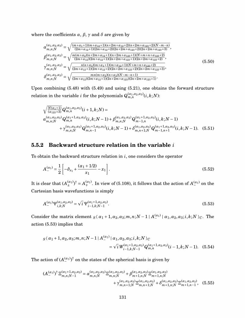
where the coefficients α, β, γ and δ are given by
α(α1,α2,α3)m,n;N =
√(m+α1+1)(m+α12+1)(n+2m+α12+2)(n+2m+α123+2)(N−m−n)
(2m+α12+1)(2m+α12+2)(2n+2m+α123+2)(2n+2m+α123+3) ,
β(α1,α2,α3)m,n;N =
√m(m+α2)(n+2m+α12+1)(n+2m+α123+1)(N+m+n+α123+2)
(2m+α12)(2m+α12+1)(2n+2m+α123+1)(2n+2m+α123+2) ,
γ(α1,α2,α3)m,n;N =
√n(n+α3)(m+α1+1)(m+α12+1)(N+m+n+α123+2)
(2m+α12+1)(2m+α12+2)(2n+2m+α123+2)(2n+2m+α123+3) ,
δ(α1,α2,α3)m,n;N =
√mn(m+α2)(n+α3)(N−m−n+1)
(2m+α12)(2m+α12+1)(2n+2m+α123)(2n+2m+α123+1) .
(5.50)
Upon combining (5.48) with (5.49) and using (5.21), one obtains the forward structure
relation in the variable i for the polynomials Q(α1,α2,α3)m,n (i,k; N):
√N(α1+1)(α123+3) Q(α1,α2,α3)
m,n (i+1,k; N)=α
(α1,α2,α3)m,n;N Q(α1+1,α2,α3)
m,n (i,k; N −1)+β(α1,α2,α3)m,n;N Q(α1+1,α2,α3)
m−1,n (i,k; N −1)
+γ(α1,α2,α3)m,n;N Q(α1+1,α2,α3)
m,n−1 (i,k; N −1)+δ(α1,α2,α3)m,n+1;N Q(α1+1,α2,α3)
m−1,n+1 (i,k; N −1). (5.51)
5.5.2 Backward structure relation in the variable i
To obtain the backward structure relation in i, one considers the operator
A(α1)− = 1
2
[−∂x1 +
(α1 +1/2)x1
− x1
]. (5.52)
It is clear that (A(α1)± )† = A(α1)
∓ . In view of (5.108), it follows that the action of A(α1)− on the
Cartesian basis wavefunctions is simply
A(α1)− Ψ
(α1,α2,α3)i,k;N =
piΨ(α1+1,α2,α3)
i−1,k;N−1 . (5.53)
Consider the matrix element S⟨ α1 +1,α2,α3;m,n; N −1 | A(α1)− | α1,α2,α3; i,k; N ⟩C. The
action (5.53) implies that
S⟨α1 +1,α2,α3;m,n; N −1 | A(α1)− |α1,α2,α3; i,k; N ⟩C
=p
iW (α1+1,α2,α3)i−1,k;N−1 Q(α1+1,α2,α3)
m,n (i−1,k; N −1). (5.54)
The action of (A(α1)− )† on the states of the spherical basis is given by
(A(α1)− )†Ξ
(α1+1,α2,α3)m,n;N−1 =α(α1,α2,α3)
m,n;N Ξ(α1,α2,α3)m,n;N +β(α1,α2,α3)
m+1,n;N Ξ(α1,α2,α3)m+1,n;N
+γ(α1,α2,α3)m,n+1;N Ξ
(α1,α2,α3)m,n+1;N +δ(α1,α2,α3)
m+1,n;N Ξ(α1,α2,α3)m+1,n−1 , (5.55)
131
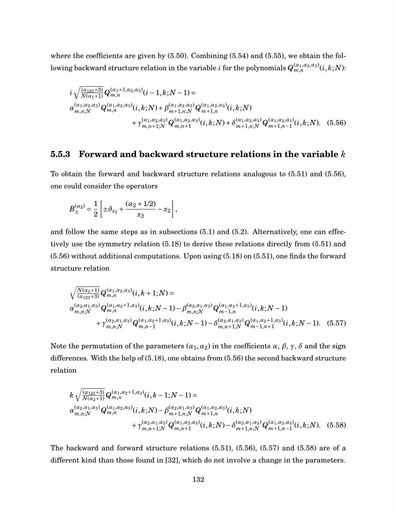
where the coefficients are given by (5.50). Combining (5.54) and (5.55), we obtain the fol-
lowing backward structure relation in the variable i for the polynomials Q(α1,α2,α3)m,n (i,k; N):
i√
(α123+3)N(α1+1) Q(α1+1,α2,α3)
m,n (i−1,k; N −1)=α
(α1,α2,α3)m,n;N Q(α1,α2,α3)
m,n (i,k; N)+β(α1,α2,α3)m+1,n;N Q(α1,α2,α3)
m+1,n (i,k; N)
+γ(α1,α2,α3)m,n+1;N Q(α1,α2,α3)
m,n+1 (i,k; N)+δ(α1,α2,α3)m+1,n;N Q(α1,α2,α3)
m+1,n−1 (i,k; N). (5.56)
5.5.3 Forward and backward structure relations in the variable k
To obtain the forward and backward structure relations analogous to (5.51) and (5.56),
one could consider the operators
B(α2)± = 1
2
[±∂x2 +
(α2 +1/2)x2
− x2
],
and follow the same steps as in subsections (5.1) and (5.2). Alternatively, one can effec-
tively use the symmetry relation (5.18) to derive these relations directly from (5.51) and
(5.56) without additional computations. Upon using (5.18) on (5.51), one finds the forward
structure relation
√N(α2+1)(α123+3) Q(α1,α2,α3)
m,n (i,k+1; N)=α
(α2,α1,α3)m,n;N Q(α1,α2+1,α3)
m,n (i,k; N −1)−β(α2,α1,α3)m,n;N Q(α1,α2+1,α3)
m−1,n (i,k; N −1)
+γ(α2,α1,α3)m,n;N Q(α1,α2+1,α3)
m,n−1 (i,k; N −1)−δ(α2,α1,α3)m,n+1;N Q(α1,α2+1,α3)
m−1,n+1 (i,k; N −1). (5.57)
Note the permutation of the parameters (α1,α2) in the coefficients α, β, γ, δ and the sign
differences. With the help of (5.18), one obtains from (5.56) the second backward structure
relation
k√
(α123+3)N(α2+1) Q(α1,α2+1,α3)
m,n (i,k−1; N −1)=α
(α2,α1,α3)m,n;N Q(α1,α2,α3)
m,n (i,k; N)−β(α2,α1,α3)m+1,n;N Q(α1,α2,α3)
m+1,n (i,k; N)
+γ(α2,α1,α3)m,n+1;N Q(α1,α2,α3)
m,n+1 (i,k; N)−δ(α2,α1,α3)m+1,n;N Q(α1,α2,α3)
m+1,n−1 (i,k; N). (5.58)
The backward and forward structure relations (5.51), (5.56), (5.57) and (5.58) are of a
different kind than those found in [32], which do not involve a change in the parameters.
132
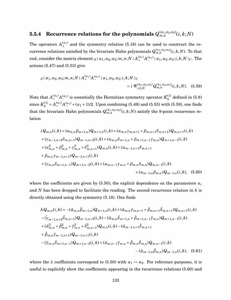
5.5.4 Recurrence relations for the polynomials Q(α1,α2,α2)m,n (i,k; N)
The operators A(α1)± and the symmetry relation (5.18) can be used to construct the re-
currence relations satisfied by the bivariate Hahn polynomials Q(α1,α2,α3)m,n (i,k; N). To that
end, consider the matrix element S⟨α1,α2,α3;m,n; N | A(α1)+ A(α1)− |α1,α2,α3; i,k; N ⟩C. The
actions (5.47) and (5.53) give
S⟨α1,α2,α3;m,n; N | A(α1)+ A(α1)
− |α1,α2,α3; i,k; N ⟩C
= i W (α1,α2,α3)i,k;N Q(α1,α2,α3)
m,n (i,k; N). (5.59)
Note that A(α1)+ A(α1)− is essentially the Hermitian symmetry operator K (1)
0 defined in (5.8)
since K (1)0 = A(α1)
+ A(α1)− + (α1+1)/2. Upon combining (5.49) and (5.55) with (5.59), one finds
that the bivariate Hahn polynomials Q(α1,α2,α3)m,n (i,k; N) satisfy the 9-point recurrence re-
lation
iQm,n(i,k)= (αm,nβm+1,n)Qm+1,n(i,k)+ (αm,nγm,n+1 +βm,n+1δm,n+1)Qm,n+1(i,k)
+ (γm−1,n+2δm,n+1)Qm−1,n+2(i,k)+ (αm,nδm+1,n +βm+1,n−1γm,n)Qm+1,n−1(i,k)
+ (α2m,n +β2
m,n +γ2m,n +δ2
m,n+1)Qm,n(i,k)+ (αm−1,n+1δm,n+1
+βm,nγm−1,n+1)Qm−1,n+1(i,k)
+ (γm,nδm+1,n−1)Qm+1,n−2(i,k)+ (αm,n−1γm,n +βm,nδm,n)Qm,n−1(i,k)
+ (αm−1,nβm,n)Qm−1,n(i,k), (5.60)
where the coefficients are given by (5.50); the explicit dependence on the parameters αi
and N has been dropped to facilitate the reading. The second recurrence relation in k is
directly obtained using the symmetry (5.18). One finds
kQm,n(i,k)=−(αm,nβm+1,n)Qm+1,n(i,k)+ (αm,nγm,n+1 + βm,n+1δm,n+1)Qm,n+1(i,k)
− ˜(γm−1,n+2δm,n+1)Qm−1,n+2(i,k)− (αm,nδm+1,n + βm+1,n−1γm,n)Qm+1,n−1(i,k)
+ (α2m,n + β2
m,n + γ2m,n + δ2
m,n+1)Qm,n(i,k)− (αm−1,n+1δm,n+1
+ βm,nγm−1,n+1)Qm−1,n+1(i,k)
− (γm,nδm+1,n−1)Qm+1,n−2(i,k)+ (αm,n−1γm,n + βm,nδm,n)Qm,n−1(i,k)
− (αm−1,nβm,n)Qm−1,n(i,k), (5.61)
where the x coefficients correspond to (5.50) with α1 ↔ α2. For reference purposes, it is
useful to explicitly show the coefficients appearing in the recurrence relations (5.60) and
133
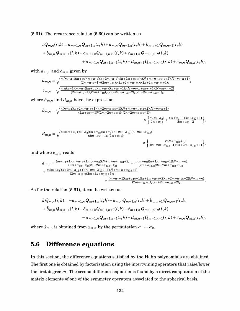
(5.61). The recurrence relation (5.60) can be written as
iQm,n(i,k)= am+1,n Qm+1,n(i,k)+am,n Qm−1,n(i,k)+bm,n+1 Qm,n+1(i,k)
+bm,n Qm,n−1(i,k)+ cm,n+2 Qm−1,n+2(i,k)+ cm+1,n Qm+1,n−2(i,k)
+dm+1,n Qm+1,n−1(i,k)+dm,n+1 Qm−1,n+1(i,k)+ em,n Qm,n(i,k),
with am,n and cm,n given by
am,n =√
m(m+α1)(m+α2)(m+α12)(n+2m+α12)2(n+2m+α123)2(N+m+n+α123+2)(N−m−n+1)(2m+α12−1)2(2m+α12)2(2n+2m+α123)2(2n+2m+α123+1)2
,
cm,n =√
m n(n−1)(m+α1)(m+α2)(m+α12)(n+α3−1)2(N+m+n+α123+1)(N−m−n+2)(2m+α12−1)2(2m+α12)2(2n+2m+α123−2)2(2n+2m+α123−1)2
,
where bm,n and dm,n have the expression
bm,n =√
n(n+α3)(n+2m+α12+1)(n+2m+α123+1)(N+m+n+α123+2)(N−m−n+1)(2m+α12+1)2(2m+2n+α123)2(2n+2m+α123+1)2
×
m(m+α2)2m+α12
+ (m+α1+1)(m+α12+1)2m+α12+2
,
dm,n =√
m n(m+α1)(m+α2)(m+α12)(n+α3)(n+2m+α12)(n+2m+α123)(2m+α12−1)2(2m+α12)2
×
(2N+α123+3)(2n+2m+α123−1)(2n+2m+α123+1)
,
and where em,n reads
em,n = (m+α1+1)(m+α12+1)n(n+α3)(N+m+n+α123+2)(2m+α12+1)2(2n+2m+α123+1)2
+ m(m+α2)(n+1)(n+α3+1)(N−m−n)(2m+α12)2(2n+2m+α123+2)2
+ m(m+α2)(n+2m+α12+1)(n+2m+α123+1)(N+m+n+α123+2)(2m+α12)2(2m+2n+α123+1)2
+ (m+α1+1)(m+α12+1)(n+2m+α12+2)(n+2m+α123+2)(N−m−n)(2m+α12+1)2(2n+2m+α123+2)2
.
As for the relation (5.61), it can be written as
kQm,n(i,k)=−am+1,n Qm+1,n(i,k)− am,n Qm−1,n(i,k)+ bm,n+1 Qm,n+1(i,k)
+ bm,n Qm,n−1(i,k)− cm,n+2 Qm−1,n+2(i,k)− cm+1,n Qm+1,n−2(i,k)
− dm+1,n Qm+1,n−1(i,k)− dm,n+1 Qm−1,n+1(i,k)+ em,n Qm,n(i,k),
where xm,n is obtained from xm,n by the permutation α1 ↔α2.
5.6 Difference equations
In this section, the difference equations satisfied by the Hahn polynomials are obtained.
The first one is obtained by factorization using the intertwining operators that raise/lower
the first degree m. The second difference equation is found by a direct computation of the
matrix elements of one of the symmetry operators associated to the spherical basis.
134
5.6.1 First difference equation
To obtain a first difference equation for the bivariate Hahn polynomials, we start from the
matrix element C⟨ α1,α2,α3; i,k : N | C(α1,α2)+ C(α1,α2)− | α1,α2,α3;m,n; N ⟩S where C(α1,α2)
±are the operators defined by (5.22) and (5.33). In view of the actions (5.23) and (5.34), it
follows that
C⟨α1,α2,α3; i,k : N | C(α1,α2)+ C(α1,α2)
− |α1,α2,α3;m,n; N ⟩S
= m(m+α12 +1)W (α1,α2,α3)i,k;N Q(α1,α2,α3)
m,n (i,k; N). (5.62)
Note that C(α1,α2)+ C(α1,α2)− is related to the operator Q(12) defined in (5.12a) since one has
C(α1,α2)+ C(α1,α2)− = Q(12) −α12(α12 +2)/4. Upon using the formulas (5.25) and (5.36) giving
the actions of C(α1,α2)± on the Cartesian basis wavefunctions, one finds
(C(α1,α2)+ C(α1,α2)
− )†Ψ(α1,α2,α3)i,k;N = [i(k+α2 +1)+k(i+α1 +1)]Ψ(α1,α2,α3)
i,k;N
−√
i(i+α1)(k+1)(k+α2 +1)Ψ(α1,α2,α3)i−1,k+1;N
−√
k(i+1)(i+α1 +1)(k+α2)Ψ(α1,α2,α3)i+1,k−1;N . (5.63)
Combining (5.62) with (5.63) and using the explicit expression (5.21) for the amplitude
W (α1,α2,α3)i,k;N , one finds that the bivariate Hahn polynomials satisfy the difference equation
m(m+α12 +1)Qm,n(i,k)= [i(k+α2 +1)+k(i+α1 +1)]Qm,n(i,k)
− i(k+α2 +1)Qm,n(i−1,k+1)
− k(i+α1 +1)Qm,n(i+1,k−1), (5.64)
where the explicit dependence on the parameters αi and N was omitted to ease the nota-
tion. Defining the operator L1 as
L1 =Υ1(i,k)T−i T+
k +Υ2(i,k)T+i T−
k − [Υ1(i,k)+Υ2(i,k)]I, (5.65)
with coefficients
Υ1(i,k)= i(k+α2 +1), Υ2(i,k)= k(i+α1 +1),
and where T±i f (i,k)= f (i±1,k) (and similarly for T±
k ) are the shift operators and I stands
for the identity operator, the difference equation (5.64) can be written as the eigenvalue
equation
L1 Q(α1,α2,α3)m,n (i,k; N)=−m(m+α12 +1)Q(α1,α2,α3)
m,n (i,k; N).
135
5.6.2 Second difference equation
It is possible to derive a second difference equation for the bivariate Hahn polynomials. To
that end, consider the matrix element C⟨α1,α2,α3; i,k; N |Q |α1,α2,α3;m,n; N ⟩S, where
Q is defined by
Q =Q(123) − (α123 +1)(α123 +3)/4,
with Q(123) given by (5.12b). It follows from (5.11) that
C⟨α1,α2,α3; i,k; N |Q |α1,α2,α3;m,n; N ⟩S
= (n+m)(n+m+α123 +2)W (α1,α2,α3)i,k;N Q(α1,α2,α3)
m,n (i,k; N). (5.66)
Upon writing Q(123) in Cartesian coordinates (see (5.14)) and acting on the Cartesian basis
wavefunctions, a straightforward calculation yields
QΨ(α1,α2,α3)i,k;N = κi,kΨ
α1,α2,α3i,k;N − σi,kΨ
(α1,α2,α3)i−1,k+1;N − ρ i,kΨ
(α1,α2,α3)i+1,k−1;N
− µi+1,kΨ(α1,α2,α3)i+1,k;N − µi,kΨ
(α1,α2,α3)i−1,k;N − νi,k+1Ψ
(α1,α2,α3)i,k+1;N − νi,kΨ
(α1,α2,α3)i,k−1;N , (5.67)
where the coefficients are of the form
κi,k = iα23 +kα13 + (N − i−k)α12 −2(i2 +k2 + i k− i N −k N −N),
σi,k =√
i(i+α1)(k+1)(k+α2 +1), ρ i,k =√
(i+1)(i+α1 +1)k(k+α2),
µi,k =√
i(i+α1)(N − i−k+1)(N − i−k+α3 +1),
νi,k =√
k(k+α2)(N − i−k+1)(N − i−k+α3 +1).
(5.68)
Combining (5.62) and (5.67) with the formula (5.21), one finds that the bivariate Hahn
polynomials Q(α1,α2,α3)m,n (i,k; N) satisfy the following difference equation:
− (n+m)(n+m+α123 +2)Qm,n(i,k)=−κi,k Qm,n(i,k)
+ i(k+α2 +1)Qm,n(i−1,k+1)+k(i+α1 +1)Qm,n(i+1,k−1)
+ (k+α2 +1)(N − i−k)Qm,n(i,k+1)+k(N − i−k+α3 +1)Qm,n(i,k−1)
+ (i+α1 +1)(N − i−k)Qm,n(i+1,k)+ i(N − i−k+α3 +1)Qm,n(i−1,k), (5.69)
where the explicit dependence on N and αi was again dropped for convenience. One can
present the difference equation (5.69) as an eigenvalue equation in the following way. We
136
define the operator
L2 =Ω1(i,k)T+i +Ω2(i,k)T+
k +Ω3(i,k)T−i +Ω4(i,k)T−
k
+Ω5(i,k)T+i T−
k +Ω6(i,k)T−i T+
k −( 6∑
j=1Ω j(i,k)
)I, (5.70)
with coefficients
Ω1(i,k)= (i+α1 +1)(N − i−k), Ω2(i,k)= (k+α2 +1)(N − i−k),
Ω3(i,k)= i(N − i−k+α3 +1), Ω4(i,k)= k(N − i−k+α3 +1),
Ω5(i,k)= k(i+α1 +1), Ω6(i,k)= i(k+α2 +1).
(5.71)
Then (5.69) assumes the form
L2 Q(α1,α2,α3)m,n (i,k; N)=−(n+m)(n+m+α123 +2)Q(α1,α2,α3)
m,n (i,k; N).
5.7 Expression in hypergeometric series
In this section, the explicit expression for the bivariate Hahn polynomials Q(α1,α2,α3)m,n in
terms of the Hahn polynomials in one variable is derived. This is done by introducing
an ancillary basis of states corresponding to the separation of variables in cylindrical
coordinates and by evaluating explicitly the Cartesian vs. cylindrical and cylindrical vs.
spherical interbasis expansion coefficients in terms of the univariate Hahn polynomials.
5.7.1 The cylindrical-polar basis
Let p and q be non-negative integers such that p ≤ q ≤ N. We shall denote by
|α1,α2,α3; p, q; N ⟩P ,
the basis vectors for the EN-energy eigenspace associated to the separation of variables
in cylindrical-polar coordinates
x1 = ρ cosϕ, x2 = ρ sinϕ, x3 = x3.
In these coordinates, the wavefunctions have the expression
⟨ ρ,ϕ, x3 |α1,α2,α3; p, q; N ⟩P =A(α1,α2,α3)p,q;N (ρ,ϕ, x3)=
η(α1,α2)p ξ
(2p+α12+1)q−p ξ
(α3)N−q G (α1,α2,α3) P (α1,α2)
p (−cos2ϕ)(ρ2)pL(2p+α12+1)q−p (ρ2)L(α3)
N−q(x23),
(5.72)
137
where the normalization factors (5.7) and (5.10) ensure that the wavefunctions (5.72)
satisfy the orthogonality condition∫ ∞
0
∫ π/2
0
∫ ∞
0
[A
(α1,α2,α3)p,q;N (ρ,ϕ, x3)
]∗A
(α1,α2,α3)p′,q′;N ′ (ρ,ϕ, x3) ρdρdϕdx3 = δpp′δqq′δNN ′ .
In Cartesian coordinates, the wavefunctions of the cylindrical basis take the form
⟨ x1, x2, x3 |α1,α2,α3; p, q; N ⟩P = η(α1,α2)p ξ
(2p+α12+1)q−p ξ
(α3)N−q G (α1,α2,α3)
(x21 + x2
2)pP (α1,α2)p
(x2
2 − x21
x21 + x2
2
)L(2m+α12+1)
q−p (x21 + x2
2)L(α3)N−q(x2
3). (5.73)
5.7.2 The cylindrical/Cartesian expansion
Let us obtain the explicit expression for the expansion coefficients P⟨p, q; N | i,k; N ⟩C
between the states of the cylindrical-polar and Cartesian bases. These expressions are al-
ready known (see for example [27]) but we give here a new derivation of these coefficients
using a generating function technique [4, 12, 17].
Upon comparing the formulas (5.6) and (5.73) for the Cartesian and cylindrical-polar
wavefunctions, it is clear that one can write
P⟨p, q; N | i,k; N ⟩C = δq,i+k P⟨p; q | i; q ⟩C,
where P⟨p; q | i; q ⟩C are the coefficients appearing in the expansion formula
ξ(α1)i ξ
(α2)q−i L(α1)
i (x21)L(α2)
q−i(x22)=
q∑p=0
P⟨p; q | i; q ⟩C
×η(α1,α2)p ξ
(2p+α12+1)q−p (x2
1 + x22)pP (α1,α2)
p
(x2
2 − x21
x21 + x2
2
)L(2p+α12+1)
q−p (x21 + x2
2). (5.74)
Since the coefficients P⟨p; q | i; q ⟩C are independent of x1, x2, the expansion formula (5.74)
holds regardless of the value taken by these coordinates, i.e. (5.74) is a formal expansion.
Let us set x21 + x2
2 = 0. Upon using the formula [2]
(x+ y)mP (α,β)m
(x− yx+ y
)= (α+1)m
m!xm
2F1
[−m,−m−βα+1
;− yx
],
and Gauss’s summation formula [2] as well as taking x22 = u, one finds that the expansion
formula (5.74) reduces to the generating relation
ξ(α1)i ξ
(α2)q−i L(α1)
i (u)L(α2)q−i(−u)
=q∑
p=0P⟨p; q | i; q ⟩C η
(α1,α2)p ξ
(2p+α12+1)q−p
(p+α12+1)p(2p+α12+2)q−p
p!(q−p)!
up.
138
The above relation can be written as
1F1
[ −iα1 +1
;−u]
1F1
[ i− qα2 +1
;u]=
i!(q−i)!
(α1+1)i(α2+1)q−i1
ξ(α1)i ξ
(α2)q−i
×q∑
p=0P⟨p; q | i; q ⟩C η
(α1,α2)p ξ
(2p+α12+1)q−p
(p+α12+1)p(2p+α12+2)q−p
p!(q−p)!
up. (5.75)
Comparing (5.75) with the generating function (5.3) of the one-variable Hahn polynomi-
als, it is easily seen that
P⟨p; q | i; q ⟩C =√ρ(i;α1,α2; q)λp(α1,α2; q)
hp(i;α1,α2; q),
where ρ(x;α,β; N) and λn(α,β; N) are respectively given by (5.1) and (5.2). The complete
expression for the overlap coefficients P⟨α1,α2,α3; p, q; N |α1,α2,α3; i,k; N ⟩C between the
states of the cylindrical and Cartesian bases is thus expressed in terms of the Hahn poly-
nomials hn(x;α,β; N) in the following way:
P⟨α1,α2,α3; p, q; N |α1,α2,α3; i,k; N ⟩C = δq,i+k
√ρ(i;α1,α2; q)λp(α1,α2; q)
hp(i;α1,α2; q). (5.76)
5.7.3 The spherical/cylindrical expansion
Upon comparing the expressions (5.13) and (5.73) giving the wavefunctions of the spheri-
cal and cylindrical-polar bases in Cartesian coordinates, it is easy to see that the overlap
coefficients S⟨m,n; N | p, q; N ⟩P between these two bases is of the form
S⟨m,n; N | p, q; N ⟩P = δmp S⟨n; N | q; N ⟩P ,
where S⟨n; N | q; N ⟩P are the coefficients arising in the expansion
ξ(2m+α12+1)q−m ξ
(α3)N−q L(2m+α12+1)
q−m (x21 + x2
2) L(α3)N−q(x2
3)
=N−m∑n=0
S⟨n; N | q; N ⟩P η(2m+α12+1,α3)n ξ
(2m+2n+α123+2)N−m−n
× (x21 + x2
2 + x23)n P (2m+α12+1,α3)
n
(x2
3 − x21 − x2
2
x21 + x2
2 + x23
)L(2m+2n+α123+2)
N−m−n (x21 + x2
2 + x23). (5.77)
Taking x21 = 0 in (5.77) and comparing with (5.74), it is easily seen that the complete
expression for the overlap coefficients between the spherical and the cylindrical-polar
139
bases are given by
S⟨α1,α2,α3;m,n; N |α1,α2,α3; p, q; N ⟩P = δmp√ρ(q−m;2m+α12 +1,α3; N −m)λn(2m+α12 +1,α3; N −m)
hn(q−m;2m+α12 +1,α3; N −m). (5.78)
5.7.4 Explicit expression for Q(α1,α2,α3)m,n (i,k; N)
The expansion formulas (5.76) and (5.78) can be combined to obtain the explicit expression
for the bivariate Hahn polynomials in terms of the univariate Hahn polynomials. Indeed,
one can write
W (α1,α2,α3)i,k;N Q(α1,α2,α3)
m,n (i,k; N)= S⟨α1,α2,α3;m,n; N |α1,α2,α3; i,k; N ⟩C
=N∑
p=0
N∑q=p
S⟨m,n; N | p, q; N ⟩P P⟨p, q; N | i,k; N ⟩C
=√ρ(i;α1,α2; i+k)λm(α1,α2; i+k)
ρ(i+k−m;2m+α12 +1,α3; N −m)λn(i+k−m;2m+α12 +1,α3; N −m)
×hm(i;α1,α2; i+ k)hn(i+ k−m;2m+α12 +1,α3; N −m). (5.79)
With the expression (5.21), one finds the following expression for Q(α1,α2,α3)m,n (i,k; N):
Q(α1,α2,α3)m,n (i,k; N)=(
Λ(α1,α2,α3)m,n;N
)−1/2hm(i;α1,α2; i+k)hn(i+k−m;2m+α12 +1,α3; N −m), (5.80)
where Λ(α1,α2,α3)m,n;N are the normalization coefficients defined in (5.45). The explicit expres-
sion (5.80) for the bivariate Hahn polynomials Q(α1,α2,α3)m,n (i,k; N) corresponds to Karlin
and McGregor’s [25]. From the results of this section, it is clear that the complete theory
of the univariate Hahn polynomials could also be worked out from their interpretation as
interbasis expansion coefficients for the two-dimensional singular oscillator.
5.8 Algebraic interpretation
In this section, an algebraic interpretation of the overlap coefficients between the Carte-
sian and spherical bases is presented in terms of su(1,1) representations. It is seen that
these overlap coefficients can be assimilated to generalized Clebsch-Gordan coefficients,
a result that entails a connection with the work of Rosengren [33].
140
5.8.1 Generalized Clebsch-Gordan problem for su(1,1)
The su(1,1) algebra has for generators the elements K0 and K± that satisfy the commu-
tation relations [16, 36]
[K0,K±]=±K±, [K−,K+]= 2K0. (5.81)
The Casimir operator C, which commutes with every generator, is of the form
C = K20 −K+K−−K0. (5.82)
Let ν > 0 be a real number and let V (ν) denote the infinite-dimensional vector space
spanned by the basis vectors e(ν)n , n ∈ 0,1, . . . , . If V (ν) is endowed with the actions
K0 e(ν)n = (n+ν) e(ν)
n ,
K+ e(ν)n =
√(n+1)(n+2ν) e(ν)
n+1,
K− e(ν)n =
√n(n+2ν−1) e(ν)
n−1,
(5.83)
then V (ν) becomes an irreducible su(1,1)-module; the representation (5.83) belongs to the
positive discrete series [36]. On this module the Casimir operator acts as a multiple of
the identity
C e(ν)n = ν(ν−1) e(ν)
n ,
as expected from Schur’s lemma. Consider three mutually commuting sets K (i)0 ,K (i)
± ,
i = 1,2,3, of su(1,1) generators. These generators can be combined as follows to produce a
fourth set of generators:
K (123)0 = K (1)
0 +K (2)0 +K (3)
0 , K (123)± = K (1)
± +K (2)± +K (3)
± .
There is a natural representation for this realization of su(1,1) on the tensor product
space V (ν1) ⊗V (ν2) ⊗V (ν3); in this representation each set of generators K (i)0 ,K (i)
± acts on
V (νi) only. A convenient basis for this module is the direct product basis spanned by the
vectors e(ν1)n1 ⊗ e(ν2)
n2 ⊗ e(ν3)n3 with the actions of the generators K (i)
0 ,K (i)± on the vectors e(νi)
ni
as prescribed by (5.83). In general, this representation is not irreducible and it can be
completely decomposed in a direct sum of irreducible representations V (ν) also belong-
ing to the positive-discrete series. To perform this decomposition, one can proceed in two
steps by first decomposing V (ν1) ⊗V (ν2) in irreducible modules V (ν12) and then decompos-
ing V (ν12) ⊗V (ν3) in irreducible modules V (ν) for each occurring values of ν12. A natural
141
basis associated to this decomposition scheme, which we shall call the “coupled” basis, is
provided by the vectors e(ν12,ν)n123 , n123 ∈ 0,1, . . ., satisfying
C(12) e(ν12,ν)n123 = ν12(ν12 −1) e(ν12,ν)
n123 ,
C(123) e(ν12,ν)n123 = ν(ν−1) e(ν12,ν)
n123 ,
K (123)0 e(ν12,ν)
n123 = (n123 +ν) e(ν12,ν)n123 ,
(5.84)
where C(12) is the Casimir operator associated to the decomposition of V (ν1) ⊗V (ν2):
C(12) = [K (12)0 ]2 −K (12)
+ K (12)− −K (12)
0 , (5.85)
with K (i j)0 = K (i)
0 +K ( j)0 , K (i j)
± = K (i)± +K ( j)
± and where C(123) is the Casimir operator associated
to the decomposition of V (ν12) ⊗V (ν3):
C(123) = [K (123)0 ]2 −K (123)
+ K (123)− −K (123)
0 . (5.86)
It is well known (see for example [5]) that the occurring values of ν12 and ν are given by
ν12(m)= m+ν1 +ν2, ν(m,n)= n+m+ν1 +ν2 +ν3, (5.87)
where m,n are non-negative integers. The direct product and coupled bases span the
same representation space and the corresponding basis vectors are thus related by a lin-
ear transformation. Furthermore, since these vectors are both eigenvectors of K (123)0 the
transformation is non-trivial if and only if the involved vectors correspond to the same
eigenvalue of K (123)0 . Let λK0 = N +ν1+ν2+ν3, N ∈ 0, . . . , N, be the eigenvalues of K (123)
0 ,
then for each N one has
e(ν1)i ⊗ e(ν2)
k ⊗ e(ν3)N−i−k =
∑m,n
m+n≤N
C(ν1,ν2,ν3)m,n (i,k; N) e(ν12(m),ν(m,n))
N−m−n , (5.88)
where i,k are positive integers such that i+ k ≤ N. The coefficients C(ν1,ν2,ν3)m,n (i,k; N) are
generalized Clebsch-Gordan coefficients for the positive-discrete series of irreducible rep-
resentations of su(1,1); the reader is referred to [5, 36] for the standard Clebsch-Gordan
problem, which involves only two representations of su(1,1).
5.8.2 Connection with the singular oscillator
The connection between the singular oscillator model and the combination of three su(1,1)
representations can be established as follows. Consider the following coordinate realiza-
142
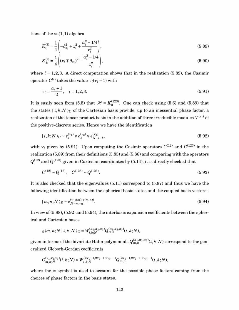
tions of the su(1,1) algebra
K (i)0 = 1
4
(−∂2
xi+ x2
i +α2
i −1/4
x2i
), (5.89)
K (i)± = 1
4
((xi ∓∂xi )
2 − α2i −1/4
x2i
), (5.90)
where i = 1,2,3. A direct computation shows that in the realization (5.89), the Casimir
operator C(i) takes the value νi(νi −1) with
νi = αi +12
, i = 1,2,3. (5.91)
It is easily seen from (5.5) that H = K (123)0 . One can check using (5.6) and (5.89) that
the states | i,k; N ⟩C of the Cartesian basis provide, up to an inessential phase factor, a
realization of the tensor product basis in the addition of three irreducible modules V (νi) of
the positive-discrete series. Hence we have the identification
| i,k; N ⟩C ∼ e(ν1)i ⊗ e(ν2)
k ⊗ e(ν3)N−i−k, (5.92)
with νi given by (5.91). Upon computing the Casimir operators C(12) and C(123) in the
realization (5.89) from their definitions (5.85) and (5.86) and comparing with the operators
Q(12) and Q(123) given in Cartesian coordinates by (5.14), it is directly checked that
C(12) ∼Q(12), C(123) ∼Q(123). (5.93)
It is also checked that the eigenvalues (5.11) correspond to (5.87) and thus we have the
following identification between the spherical basis states and the coupled basis vectors:
| m,n; N ⟩S ∼ e(ν12(m),ν(m,n))N−m−n . (5.94)
In view of (5.88), (5.92) and (5.94), the interbasis expansion coefficients between the spher-
ical and Cartesian bases
S⟨m,n; N | i,k; N ⟩C =W (α1,α2,α3)i,k;N Q(α1,α2,α3)
m,n (i,k; N),
given in terms of the bivariate Hahn polynomials Q(α1,α2,α3)m,n (i,k; N) correspond to the gen-
eralized Clebsch-Gordan coefficients
C(ν1,ν2,ν3)m,n;N (i,k; N)'W (2ν1−1,2ν2−1,2ν3−1)
i,k;N Q(2ν1−1,2ν2−1,2ν3−1)m,n (i,k; N),
where the ' symbol is used to account for the possible phase factors coming from the
choices of phase factors in the basis states.
143
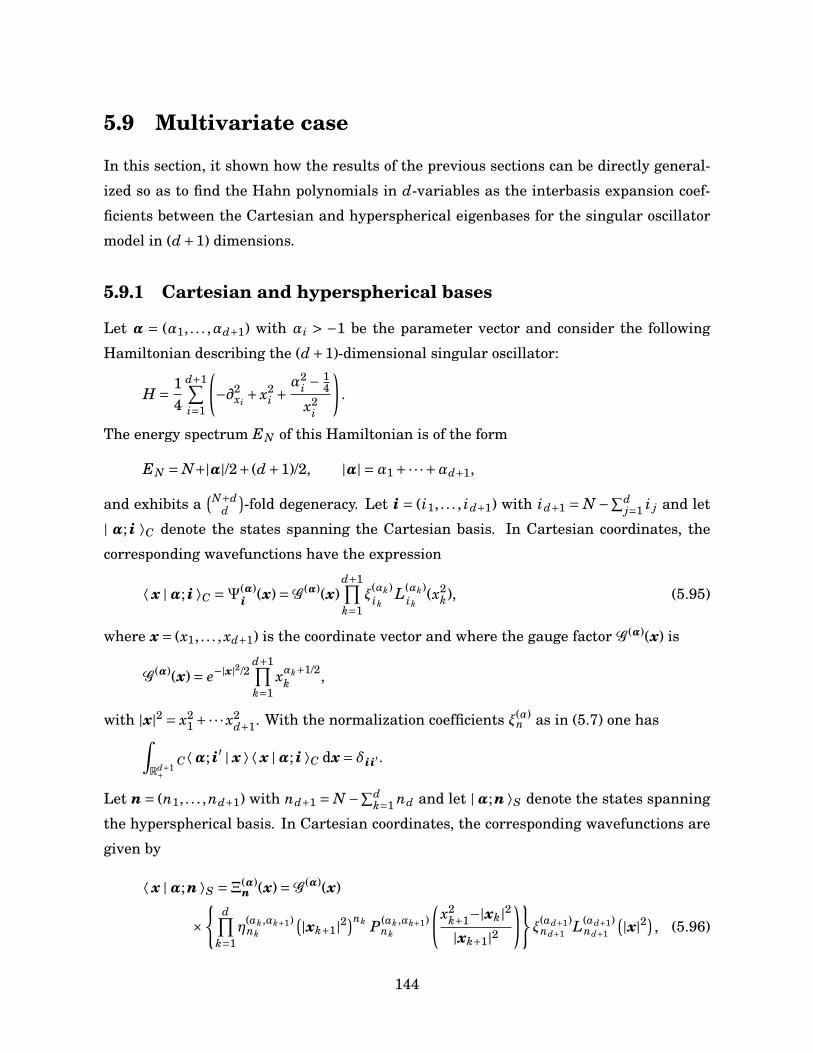
5.9 Multivariate case
In this section, it shown how the results of the previous sections can be directly general-
ized so as to find the Hahn polynomials in d-variables as the interbasis expansion coef-
ficients between the Cartesian and hyperspherical eigenbases for the singular oscillator
model in (d+1) dimensions.
5.9.1 Cartesian and hyperspherical bases
Let α = (α1, . . . ,αd+1) with αi > −1 be the parameter vector and consider the following
Hamiltonian describing the (d+1)-dimensional singular oscillator:
H = 14
d+1∑i=1
(−∂2
xi+ x2
i +α2
i − 14
x2i
).
The energy spectrum EN of this Hamiltonian is of the form
EN = N+|α|/2+ (d+1)/2, |α| =α1 +·· ·+αd+1,
and exhibits a(N+d
d)-fold degeneracy. Let i = (i1, . . . , id+1) with id+1 = N −∑d
j=1 i j and let
| α; i ⟩C denote the states spanning the Cartesian basis. In Cartesian coordinates, the
corresponding wavefunctions have the expression
⟨ x |α; i ⟩C =Ψ(α)i (x)=G (α)(x)
d+1∏k=1
ξ(αk)ik
L(αk)ik
(x2k), (5.95)
where x= (x1, . . . , xd+1) is the coordinate vector and where the gauge factor G (α)(x) is
G (α)(x)= e−|x|2/2
d+1∏k=1
xαk+1/2k ,
with |x|2 = x21 +·· ·x2
d+1. With the normalization coefficients ξ(α)n as in (5.7) one has∫
Rd+1+C⟨α; i′ | x ⟩⟨ x |α; i ⟩C dx= δii′ .
Let n = (n1, . . . ,nd+1) with nd+1 = N −∑dk=1 nd and let |α;n ⟩S denote the states spanning
the hyperspherical basis. In Cartesian coordinates, the corresponding wavefunctions are
given by
⟨ x |α;n ⟩S =Ξ(α)n (x)=G (α)(x)
×
d∏k=1
η(ak,αk+1)nk
(|xk+1|2)nk P (ak,αk+1)
nk
(x2
k+1−|xk|2|xk+1|2
)ξ
(ad+1)nd+1 L(ad+1)
nd+1
(|x|2) , (5.96)
144
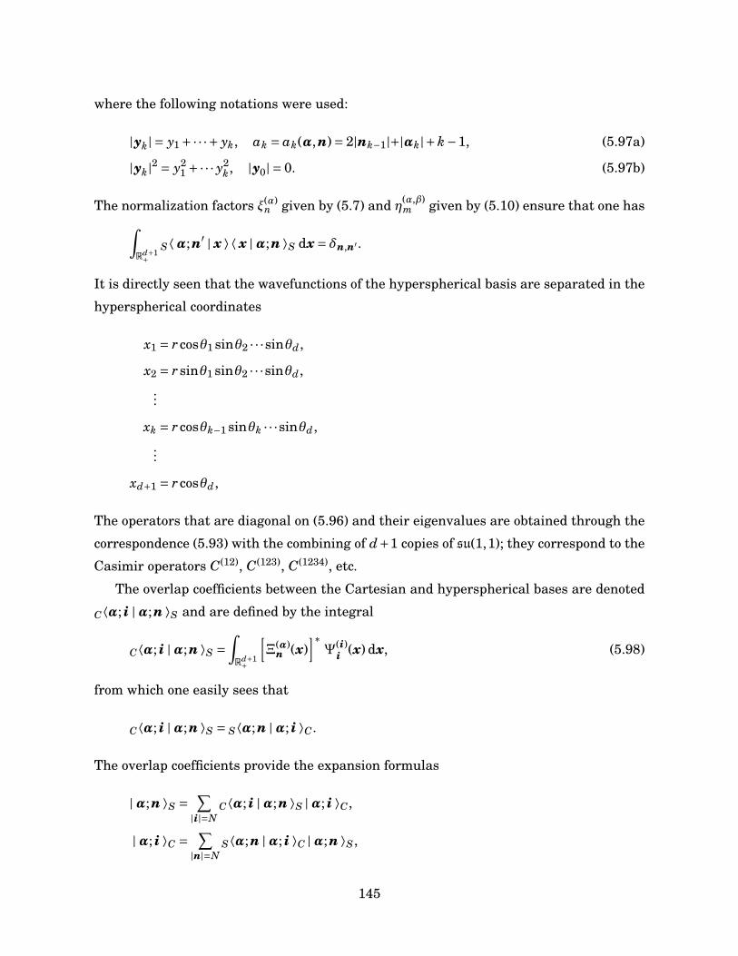
where the following notations were used:
|yk| = y1 +·· ·+ yk, ak = ak(α,n)= 2|nk−1|+|αk|+k−1, (5.97a)
|yk|2 = y21 +·· · y2
k, |y0| = 0. (5.97b)
The normalization factors ξ(α)n given by (5.7) and η(α,β)
m given by (5.10) ensure that one has∫Rd+1+
S⟨α;n′ | x ⟩⟨ x |α;n ⟩S dx= δn,n′ .
It is directly seen that the wavefunctions of the hyperspherical basis are separated in the
hyperspherical coordinates
x1 = r cosθ1 sinθ2 · · ·sinθd,
x2 = rsinθ1 sinθ2 · · ·sinθd,...
xk = r cosθk−1 sinθk · · ·sinθd,...
xd+1 = r cosθd,
The operators that are diagonal on (5.96) and their eigenvalues are obtained through the
correspondence (5.93) with the combining of d+1 copies of su(1,1); they correspond to the
Casimir operators C(12), C(123), C(1234), etc.
The overlap coefficients between the Cartesian and hyperspherical bases are denoted
C⟨α; i |α;n ⟩S and are defined by the integral
C⟨α; i |α;n ⟩S =∫Rd+1+
[Ξ(α)
n (x)]∗Ψ(i)
i (x) dx, (5.98)
from which one easily sees that
C⟨α; i |α;n ⟩S = S⟨α;n |α; i ⟩C.
The overlap coefficients provide the expansion formulas
|α;n ⟩S = ∑|i|=N
C⟨α; i |α;n ⟩S |α; i ⟩C,
|α; i ⟩C = ∑|n|=N
S⟨α;n |α; i ⟩C |α;n ⟩S,
145
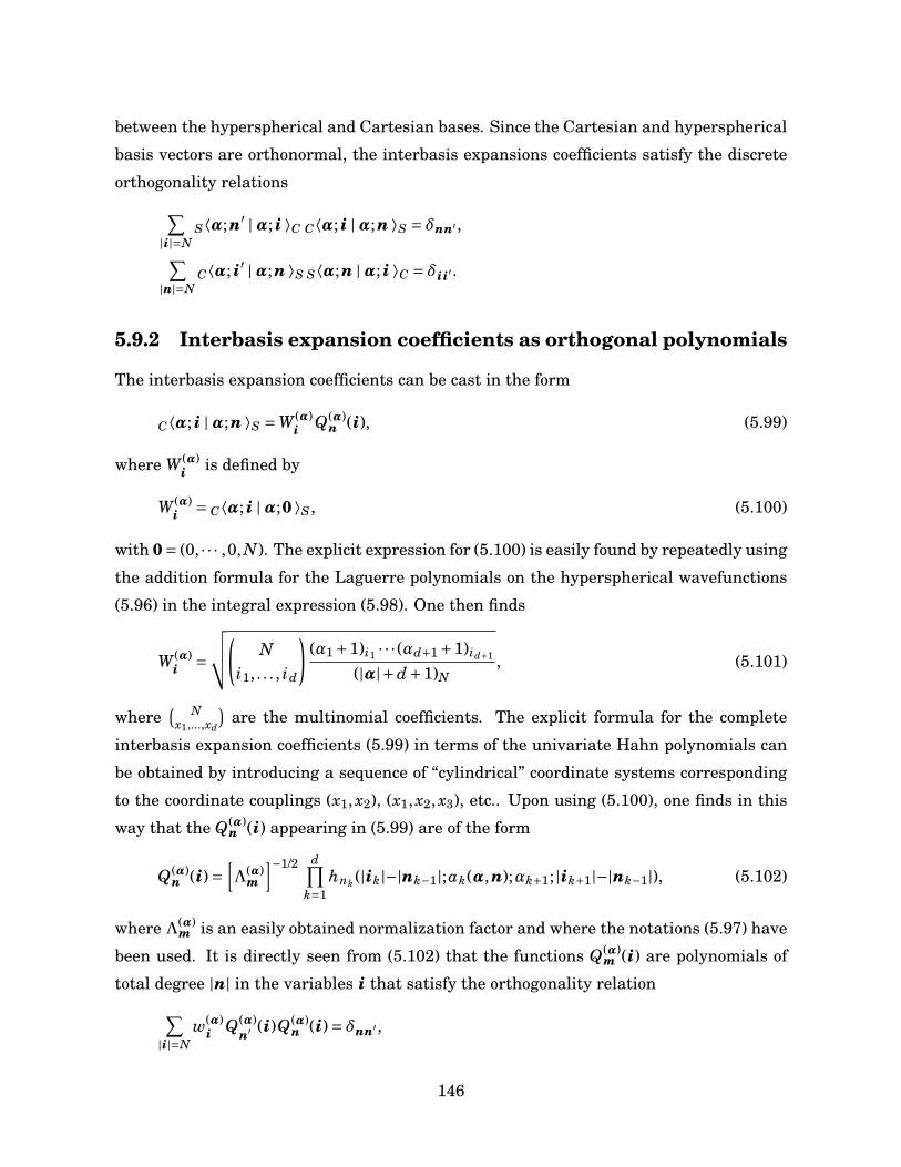
between the hyperspherical and Cartesian bases. Since the Cartesian and hyperspherical
basis vectors are orthonormal, the interbasis expansions coefficients satisfy the discrete
orthogonality relations∑|i|=N
S⟨α;n′ |α; i ⟩C C⟨α; i |α;n ⟩S = δnn′ ,
∑|n|=N
C⟨α; i′ |α;n ⟩S S⟨α;n |α; i ⟩C = δii′ .
5.9.2 Interbasis expansion coefficients as orthogonal polynomials
The interbasis expansion coefficients can be cast in the form
C⟨α; i |α;n ⟩S =W (α)i Q(α)
n (i), (5.99)
where W (α)i is defined by
W (α)i = C⟨α; i |α;0 ⟩S, (5.100)
with 0= (0, · · · ,0, N). The explicit expression for (5.100) is easily found by repeatedly using
the addition formula for the Laguerre polynomials on the hyperspherical wavefunctions
(5.96) in the integral expression (5.98). One then finds
W (α)i =
√√√√(N
i1, . . . , id
)(α1 +1)i1 · · · (αd+1 +1)id+1
(|α|+d+1)N, (5.101)
where( Nx1,...,xd
)are the multinomial coefficients. The explicit formula for the complete
interbasis expansion coefficients (5.99) in terms of the univariate Hahn polynomials can
be obtained by introducing a sequence of “cylindrical” coordinate systems corresponding
to the coordinate couplings (x1, x2), (x1, x2, x3), etc.. Upon using (5.100), one finds in this
way that the Q(α)n (i) appearing in (5.99) are of the form
Q(α)n (i)=
[Λ(α)
m
]−1/2 d∏k=1
hnk (|ik|−|nk−1|;ak(α,n);αk+1; |ik+1|−|nk−1|), (5.102)
where Λ(α)m is an easily obtained normalization factor and where the notations (5.97) have
been used. It is directly seen from (5.102) that the functions Q(α)m (i) are polynomials of
total degree |n| in the variables i that satisfy the orthogonality relation∑|i|=N
w(α)i Q(α)
n′ (i)Q(α)n (i)= δnn′ ,
146
with respect to the multivariate hypergeometric distribution
w(α)i =
[W (α)
i
]2 =∏d+1
k=1
(ik+αkik
)(N+|α|+d
N) .
The properties of the multivariate Hahn polynomials Q(α)n (i) can be derived using the
same methods as in the previous sections.
5.10 Conclusion
In this paper, we have shown that Karlin and McGregor’s d-variable Hahn polynomi-
als arise as interbasis expansion coefficients in the (d +1)-dimensional singular oscilla-
tor model. Using the framework provided by this interpretation, the main properties of
the bivariate polynomials were obtained: explicit expression in univariate Hahn polyno-
mials, recurrence relations, difference equations, generating function, raising/lowering
relations, etc. The connection between our approach and the combining of su(1,1) repre-
sentations was also established.
A natural question that arises from our considerations is whether a similar interpre-
tation can be given for the multivariate Racah polynomials, which have one parameter
more than the multivariate Hahn polynomials. The answer to that question is in the
positive. Indeed, the multivariate Racah polynomials can be seen to occur as interbasis
expansion coefficients in the so-called generic (d +1)-parameter model on the d-sphere.
With the usual embedding x21 + ·· · + x2
d+1 = 1 of the d-sphere in the (d +1)-dimensional
Euclidean plane, this model is described by the Hamiltonian
H = ∑0≤i< j≤d+1
[1i(xi∂x j − x j∂xi
)]2+
d+1∑k=1
α2k −1/4
x2k
,
and the (d−1)-variate Racah polynomials arise as the overlap coefficients between bases
associated to the separation of variables different hyperspherical coordinate systems. In
the d = 2 and d = 3 cases, this result is contained (in a hidden way) in the papers [23]
and [22] of Kalnins, Miller and Post; these papers focus on the representations of the
symmetry algebra. We shall soon report on the characterization of the multivariate Racah
polynomials using their interpretation as interbasis expansion coefficients for the generic
(d+1)-parameter system on the d-sphere.
147
5.A A compendium of formulas for
the bivariate Hahn polynomials
In this appendix we give for reference a compendium of formulas for the bivariate Hahn
polynomials; some of them can be found in the literature, others not as far as we know.
Recall that the univariate Hahn polynomials hn(x;α,β; N) are defined by
hn(x;α,β; N)= (α+1)n(−N)n 3F2
[−n,n+α+β+1,−xα+1,−N
;1],
where pFq is the generalized hypergeometric function [2].
5.A.1 Definition
The bivariate Hahn polynomials P(α1,α2,α3)n1,n2 (x1, x2; N) are defined by
P(α1,α2,α3)n1,n2 (x1, x2; N)=
1(−N)n1+n2
hn1(x1;α1,α2; x1 + x2) hn2(x1 + x2 −n1;2n1 +α1 +α2 +1,α3; N −n1).
It is checked that P(α1,α2,α3)n1,n2 (x1, x2; N) are polynomials of total degree n1 +n2 in the vari-
ables x1 and x2.
5.A.2 Orthogonality
The polynomials P(α1,α2,α3)n1,n2 (x1, x2; N) satisfy the orthogonality relation
∑x1,x2
x1+x2≤N
ω(α1,α2,α3)x1,x2;N P
(α1,α2,α3)n1,n2 (x1, x2; N)P (α1,α2,α3)
m1,m2 (x1, x2; N)=λ(α1,α2,α3)n1,n2;N δm1,n1δm2,n2 .
The orthogonality weight ω(α1,α2,α3)x1,x2;N is given by
ω(α1,α2,α3)x1,x2;N =
(x1+α1x1
)(x2+α2x2
)(N−x1−x2+α3N−x1−x2
)(N+α1+α2+α3+2
N) ,
and the normalization factor λ(α1,α2,α3)n1,n2;N reads
λ(α1,α2,α3)n1,n2;N = n1!n2!(N−n1−n2)!
N!(α1+1)n1 (α2+1)n1 (α3+1)n2 (α1+α2+1)2n1
(α1+α2+1)n1 (α1+α2+α3+3)N
× (2n1+α1+α2+2)n2 (2n1+α1+α2+α3+2)2n2 (n1+n2+α1+α2+α3+3)N(2n1+α1+α2+α3+2)n2 (n1+n2+α1+α2+α3+3)n1+n2
.
148

5.A.3 Recurrence relations
The bivariate Hahn polynomials Pn1,n2(x1, x2) satisfy the recurrence relation
x1Pn1,n2(x1, x2)= an1,n2 Pn1+1,n2(x1, x2)+bn1,n2 Pn1,n2+1(x1, x2)
+ cn1,n2 Pn1−1,n2+2(x1, x2)+dn1,n2 Pn1−1,n2+1(x1, x2)+ en1,n2 Pn1,n2(x1, x2)
+ fn1,n2 Pn1+1,n2−1(x1, x2)− gn1,n2 Pn1+1,n2−2(x1, x2)
−hn1,n2 Pn1,n2−1(x1, x2)− in1,n2 Pn1−1,n2(x1, x2),
where the coefficients are given by
an1,n2 = (n1+α1+α2+1)(2n1+n2+α1+α2+α3+2)(2n1+n2+α1+α2+α3+3)(n1+n2−N)(2n1+α1+α2+1)(2n1+α1+α2+2)(2n1+2n2+α1+α2+α3+2)(2n1+2n2+α1+α2+α3+3) ,
bn1,n2 =(2n1+n2+α1+α2+α3+2)[2n2
1+2n1(α1+α2+1)+(α1+1)(α1+α2)](n1+n2−N)(2n1+α1+α2)(2n1+α1+α2+2)(2n1+2n2+α1+α2+α3+2)(2n1+2n2+α1+α2+α3+3) ,
cn1,n2 = n1(n1+α1)(n1+α2)(n1+n2−N)(2n1+α1+α2)(2n1+α1+α2+1)(2n1+2n2+α1+α2+α3+2)(2n1+2n2+α1+α2+α3+3) ,
dn1,n2 = n1(n1+α1)(n1+α2)(2n1+n2+α1+α2+1)(2N+α1+α2+α3+3)(2n1+α1+α2)(2n1+α1+α2+1)(2n1+2n2+α1+α2+α3+1)(2n1+2n2+α1+α2+α3+3) ,
fn1,n2 = n2(n2+α3)(n1+α1+α2+1)(2n1+n2+α1+α2+α3+2)(2N+α1+α2+α3+3)(2n1+α1+α2+1)(2n1+α1+α2+2)(2n1+2n2+α1+α2+α3+1)(2n1+2n2+α1+α2+α3+3) ,
gn1,n2 = n2(n2−1)(n2+α3)(n2+α3−1)(n1+α1+α2+1)(N+n1+n2+α1+α2+α3+2)(2n1+α1+α2+1)(2n1+α1+α2+2)(2n1+2n2+α1+α2+α3+1)(2n1+2n2+α1+α2+α3+2) ,
hn1,n2 =n2(n2+α3)(2n2
1+2n1(α1+α2+1)+(α1+1)(α1+α2))(2n1+n2+α1+α2+1)(N+n1+n2+α1+α2+α3+2)(2n1+α1+α2)(2n1+α1+α2+2)(2n1+2n2+α1+α2+α3+1)(2n1+2n2+α1+α2+α3+2) ,
in1,n2 = n1(n1+α1)(n1+α2)(2n1+n2+α1+α2)(2n1+n2+α1+α2+1)(N+n1+n2+α1+α2+α3+2)(2n1+α1+α2)(2n1+α1+α2+1)(2n1+2n2+α1+α2+α3+1)(2n1+2n2+α1+α2+α3+2) ,
and by
en1,n2 = n2(n1+α1+1)(n1+α1+α2+1)(n2+α3)(N+n1+n2+α1+α2+α3+2)(2n1+α1+α2+1)(2n1+α1+α2+2)(2n1+2n2+α1+α2+α3+1)(2n1+2n2+α1+α2+α3+2)
+ n1(n1+α2)(n2+1)(n2+α3+1)(N−n1−n2)(2n1+α1+α2)(2n1+α1+α2+1)(2n1+2n2+α1+α2+α3+2)(2n1+2n2+α1+α2+α3+3)
+ n1(n1+α2)(2n1+n2+α1+α2+1)(2n1+n2+α1+α2+α3+1)(N+n1+n2+α1+α2+α3+2)(2m+α12)2(2m+2n+α123+1)2
+ (n1+α1+1)(n1+α1+α2+1)(2n1+n2+α1+α2+2)(2n1+n2+α1+α2+α3+2)(N−n1−n2)(2n1+α1+α2+1)(2n1+α1+α2+2)(2n1+2n2+α1+α2+α3+2)(2n1+2n2+α1+α2+α3+3) .
The bivariate Hahn polynomials also satisfy the recurrence relation
x2Pn1,n2(x1, x2)=−an1,n2 Pn1+1,n2(x1, x2)+ bn1,n2 Pn1,n2+1(x1, x2)
− cn1,n2 Pn1−1,n2+2(x1, x2)− dn1,n2 Pn1−1,n2+1(x1, x2)+ en1,n2 Pn1,n2(x1, x2)
− fn1,n2 Pn1+1,n2−1(x1, x2)+ gn1,n2 Pn1+1,n2−2(x1, x2)
− hn1,n2 Pn1,n2−1(x1, x2)+ in1,n2 Pn1−1,n2(x1, x2),
where the coefficients yn1,n2 are obtained from yn1,n2 by the permutation α1 ↔α2
149
5.A.4 Difference equations
The bivariate Hahn polynomials P(α1,α2,α3)n1,n2 (x1, x2; N) satisfy the eigenvalues equation
L1 P(α1,α2,α3)n1,n2 (x1, x2; N)=−n1(n1 +α1 +α2 +1)P (α1,α2,α3)
n1,n2 (x1, x2; N)
where
L1 = x1(x2 +α2 +1)T−x1
T+x2+ x2(x1 +α1 +1)T+
x1T−
x2
− (x1(x2 +α2 +1)+ x2(x1 +α1 +1))I,
where T±xi
are the usual forward and backward shift operators in the variable xi. The
bivariate Hahn polynomials also satisfy
L2 P(α1,α2,α3)n1,n2 (x1, x2; N)=
− (n1 +n2)(n1 +n2 +α1 +α2 +α3 +2)P (α1,α2,α3)n1,n2 (x1, x2; N),
where L2 is the difference operator
L2 = (N − x1 − x2)[(x1 +α1 +1)T+
x1+ (x2 +α2 +1)T+
x2
]+ x1(x2 +α2 +1)T−x1
T+x2
+ (N − x1 − x2 +α3 +1)[x1T−
x1+ x2T−
x2
]+ x2(x1 +α1 +1)T+x1
T−x2
−[(N − x1 − x2)(x1 + x2 +α1 +α2 +2)+ (x1 + x2)(N − x1 − x2 +α3 +1)
+ x1(x2 +α2 +1)+ x2(x1 +α1 +1)]I.
5.A.5 Generating Function
The polynomials P(α1,α2,α3)n1,n2 (x1, x2; N) have for generating function
(1+ z1 + z2)N−n1 (z1 + z2)n1 P (α1,α2)n1
(z2 − z1
z1 + z2
)P (2n1+α1+α2+1,α3)
n2
(1− z1 − z2
1+ z1 + z2
)= ∑
x1,x2x1+x2≤N
N!x1!x2!(N − x1 − x2)!
P(α1,α2,α3)n1,n2 (x1, x2; N)
n1!n2!zx1
1 zx22 .
5.A.6 Forward shift operators
One has the forward relation
−N P(α1,α2,α3)n1+1,n2
(x1, x2; N)= x1(x2 +α2 +1)P (α1+1,α2+1,α3)n1,n2 (x1 −1, x2; N −1)
− x2(x1 +α1 +1)P (α1+1,α2+1,α3)n1,n2 (x1, x2 −1; N −1),
150
and
−N(n2 +α3 +2)P (α1,α2,α3)n1,n2+1 (x1, x2; N)=
(x1 +α1 +1)(N − x1 − x2)(N − x1 − x2 −1)P (α1,α2,α3+2)n1,n2 (x1 +1, x2; N −1)
+ (x2 +α2 +1)(N − x1 − x2)(N − x1 − x2 −1)P (α1,α2,α3+2)n1,n2 (x1, x2 +1; N −1)
+ x1(N − x1 − x2 +α3 +1)(N − x1 − x2 +α3 +2)P (α1,α2,α3+2)n1,n2 (x1 −1, x2; N −1)
+ x2(N − x1 − x2 +α3 +1)(N − x1 − x2 +α3 +2)P (α1,α2,α3+2)n1,n2 (x1, x2 −1; N −1)
− (N−x1−x2)(N−x1−x2+α3+1)(2x1+2x2+α1+α2+2)P (α1,α2,α3+2)n1,n2 (x1, x2; N−1).
These relations can be used to generate the polynomials recursively.
5.A.7 Backward shift operators
The backward relations are given by
− n1(n1+α1+α2+1)N+1 P
(α1+1,α2+1,α3)n1−1,n2
(x1, x2; N)=P
(α1,α2,α3)n1,n2 (x1 +1, x2; N +1)−P
(α1,α2,α3)n1,n2 (x1, x2 +1; N +1),
and
− n2(2n1+n2+α1+α2+1)(2n1+n2+α1+α2+α3+2)N+1 P
(α1,α2,α3+2)n1,n2−1 (x1, x2; N)=
(x1 +α1 +1)P (α1,α2,α3)n1,n2 (x1 +1, x2; N +1)+ x1 P
(α1,α2,α3)n1,n2 (x1 −1, x2; N +1)
+ (x2 +α2 +1)P (α1,α2,α3)n1,n2 (x1, x2 +1; N +1)+ x2 P
(α1,α2,α3)n1,n2 (x1, x2 −1; N +1)
− (2x1 +2x2 +α1 +α2 +2)P (α1,α2,α3)n1,n2 (x1, x2; N +1).
5.A.8 Structure relations
One has
N P(α1,α2,α3)n1,n2 (x1 +1, x2; N)=
(n1+α1+α2+1)(2n1+n2+α1+α2+α3+2)(N−n1−n2)(2n1+α1+α2+1)(2n1+2n2+α1+α2+α3+2) P
(α1+1,α2,α3)n1,n2 (x1, x2; N −1)
− n1(n1+α2)(2n1+n2+α1+α2+1)(N+n1+n2+α1+α2+α3+2)(2n1+α1+α2+1)(2n1+2n2+α1+α2+α3+2) P
(α1+1,α2,α3)n1−1,n2
(x1, x2; N −1)
− n2(n2+α3)(n1+α1+α2+1)(N+n1+n2+α1+α2+α3+2)(2n1+α1+α2+1)(2n1+2n2+α1+α2+α3+2) P
(α1+1,α2,α3)n1,n2−1 (x1, x2; N −1)
+ n1(n1+α2)(N−n1−n2)(2n1+α1+α2+1)(2n1+2n2+α1+α2+α3+2) P
(α1+1,α2,α3)n1−1,n2+1 (x1, x2; N −1).
151
Since P(α1,α2,α3)n1,n2 (x1, x2; N)= (−1)n1P
(α2,α1,α3)n1,n2 (x2, x1; N), we also have
N P(α1,α2,α3)n1,n2 (x1, x2 +1; N)=
(n1+α1+α2+1)(2n1+n2+α1+α2+α3+2)(N−n1−n2)(2n1+α1+α2+1)(2n1+2n2+α1+α2+α3+2) P
(α1,α2+1,α3)n1,n2 (x1, x2; N −1)
+ n1(n1+α1)(2n1+n2+α1+α2+1)(N+n1+n2+α1+α2+α3+2)(2n1+α1+α2+1)(2n1+2n2+α1+α2+α3+2) P
(α1,α2+1,α3)n1−1,n2
(x1, x2; N −1)
− n2(n2+α3)(n1+α1+α2+1)(N+n1+n2+α1+α2+α3+2)(2n1+α1+α2+1)(2n1+2n2+α1+α2+α3+2) P
(α1,α2+1,α3)n1,n2−1 (x1, x2; N −1)
− n1(n1+α1)(N−n1−n2)(2n1+α1+α2+1)(2n1+2n2+α1+α2+α3+2) P
(α1,α2+1,α3)n1−1,n2+1 (x1, x2; N −1).
Another set of structure relations is the following:
x1
NP
(α1+1,α2,α3)n1,n2 (x1 −1, x2; N −1)=
(n1+α1+1)(2n1+n2+α1+α2+2)(2n1+α1+α2+2)(2n1+2n2+α1+α2+α3+3) P
(α1,α2,α3)n1,n2 (x1, x2; N)
− (2n1+n2+α1+α2+α3+3)(2n1+α1+α2+2)(2n1+2n2+α1+α2+α3+3) P
(α1,α2,α3)n1+1,n2
(x1, x2; N)
− (n1+α1+1)(2n1+α1+α2+2)(2n1+2n2+α1+α2+α3+3)P
(α1,α2,α3)n1,n2+1 (x1, x2; N)
+ n2(n2+α3)(2n1+α1+α2+2)(2n1+2n2+α1+α2+α3+3)P
(α1,α2,α3)n1+1,n2−1(x1, x2; N).
x2
NP
(α1,α2+1,α3)n1,n2 (x1, x2 −1; N −1)=
(n1+α2+1)(2n1+n2+α1+α2+2)(2n1+α1+α2+2)(2n1+2n2+α1+α2+α3+3) P
(α1,α2,α3)n1,n2 (x1, x2; N)
+ (2n1+n2+α1+α2+α3+3)(2n1+α1+α2+2)(2n1+2n2+α1+α2+α3+3) P
(α1,α2,α3)n1+1,n2
(x1, x2; N)
− (n1+α2+1)(2n1+α1+α2+2)(2n1+2n2+α1+α2+α3+3)P
(α1,α2,α3)n1,n2+1 (x1, x2; N)
− n2(n2+α3)(2n1+α1+α2+2)(2n1+2n2+α1+α2+α3+3)P
(α1,α2,α3)n1+1,n2−1(x1, x2; N).
5.B Structure relations for Jacobi polynomials
The Jacobi polynomials P (α,β)n (z) are defined by [28]
P (α,β)n (z)= (α+1)n
n! 2F1
[−n,n+α+β+1α+1
;1− z
2
]. (5.103)
The following structure relations hold for the Jacobi polynomials [29]:
∂zP (α,β)n (z)= (n+α+β+1)
2P (α+1,β+1)
n−1 (z), (5.104)
[(z−1)∂2
z + (α+1)∂z]P (α,β)
n (z)= (n+α)(n+α+β+1)2
P (α,β+2)n−1 (z), (5.105)
152
[(1− z2)∂z + [(β−α)− (α+β)z]
]P (α,β)
n (z)=−2(n+1)P (α−1,β−1)n+1 (z), (5.106)
(1+ z)(z2 −1)∂2
z + (1+ z)[1+α−2β+ (1+α+2β)z]∂z
+β[2+α(1+ z)+β(z−1)]P (α,β)
n (z)= 2(n+1)(n+β)P (α,β−2)n+1 (z). (5.107)
5.C Structure relations for Laguerre polynomials
The Laguerre polynomials L(α)n (z) are defined by
L(α)n (z)= (α+1)n
n! 1F1
[ −nα+1
; z].
The following structure relations hold for the Laguerre polynomials [28]:
∂zL(α)n (z)=−L(α+1)
n−1 (z), (5.108)
[z∂z + (α− z)]L(α)n (z)= (n+1)L(α−1)
n+1 (z). (5.109)
References
[1] C. Albanese, M. Christandl, N. Datta, and A. Ekert. Mirror Inversion of Quantum States in
Linear Registers. Phys. Rev. Lett., 93:230502, 2004.
[2] G. Andrews, R. Askey, and R. Roy. Special functions. Cambridge University Press, 1999.
[3] R. Chakrabarti and J. Van der Jeugt. Quantum communication through a spin chain with
interaction determined by a Jacobi matrix. J. Phys. A: Math. Theor., 438:085302, 2010.
[4] J. Van der Jeugt. Coupling coefficients for Lie algebra representations and addition formulas
for special functions. J. Math. Phys., 38:2728, 1997.
[5] J. Van der Jeugt. 3n j-Coefficients and Orthogonal Polynomials of Hypergeometric Type.
In E. Koelink and W. Van Assche, editors, Orthogonal Polynomials and Special Functions,
Lecture Notes in Mathematics Vol. 1817. Springer, 2003.
[6] J. J. Duistermaat and A. Grünbaum. Differential equations in the spectral parameter. Comm.
Math. Phys., 103:177–240, 1986.
153
[7] C. F. Dunkl. A difference equation and Hahn polynomials in two variables. Pac. J. Math.,
92:57–71, 1981.
[8] C. F. Dunkl and Y. Xu. Orthogonal Polynomials of Several Variables. Cambridge University
Press, 2001.
[9] G. Gasper and M. Rahman. Some systems of multivariable orthogonal q-Racah polynomials.
Ramanujan J., 13:389–405, 2007.
[10] V. X. Genest, H. Miki, L. Vinet, and A. Zhedanov. The multivariate Charlier polynomials as
matrix elements of the Euclidean group representation on oscillator states. J. Phys. A: Math.
Theor., 47:215204, 2014.
[11] V. X. Genest, H. Miki, L. Vinet, and A. Zhedanov. The multivariate Meixner polynomials as
matrix elements of SO(d,1) representations on oscillator states. J. Phys. A: Math. Theor.,
47:045207, 2014.
[12] V. X. Genest and L. Vinet. The generic superintegrable system on the 3-sphere and the 9 j
symbols of su(1,1). SIGMA, 10:108, 2014.
[13] V. X. Genest, L. Vinet, and A. Zhedanov. The multivariate Krawtchouk polynomials as matrix
elements of the rotation group representations on oscillator states. J. Phys. A: Math. Theor.,
46:505203, 2013.
[14] V. X. Genest, L. Vinet, and A. Zhedanov. Interbasis expansions for the isotropic 3D harmonic
oscillator and bivariate Krawtchouk polynomials. J. Phys. A: Math. Theor., 47:025202, 2014.
[15] J. S. Geronimo and P. Iliev. Bispectrality of multivariable Racah-Wilson polynomials. Constr.
Approx., 311:417–457, 2010.
[16] R. Gilmore. Lie groups, Lie algebras and some of their applications. Dover Publications, 2006.
[17] Ya. A. Granovskii and A. Zhedanov. New construction of 3n j symbols. J. Phys. A: Math. Gen.,
26:4339, 1993.
[18] R. C. Griffiths and D. Spano. Orthogonal polynomial kernels and canonical correlations for
Dirichlet measures. Bernoulli, 19:548–598, 2013.
[19] P. Iliev. Bispectral commuting difference operators for multivariable Askey-Wilson polyno-
mials. Trans. Amer. Math. Soc., 363:1577–1598, 2011.
[20] P. Iliev and Y. Xu. Discrete orthogonal polynomials and difference equations of several vari-
ables. Adv. Math., 212:1–36, 2007.
154
[21] M.E.H. Ismail. Classical and Quantum Orthogonal Polynomials in one variable, volume 98
of Encyclopedia of Mathematics and its Applications. Cambridge University Press, 2005.
[22] E. G. Kalnins, W. Miller, and S. Post. Two-variable Wilson polynomials and the generic
superintegrable system on the 3-sphere. SIGMA, 7:51–76, 2011.
[23] E.G. Kalnins, W. Miller, and S. Post. Wilson polynomials and the generic superintegrable
system on the 2-sphere. J. Phys. A: Math. Theor., 40:11525–11538, 2007.
[24] S. Karlin and J. McGregor. The Hahn polynomials, formulas and an application. Scrpt. Math.,
26:33–46, 1961.
[25] S. Karlin and J. McGregor. Linear growth models with many types and multidimensional
Hahn polynomials. In R. Askey, editor, Theory and Applications of Special Functions, pages
261–288. Academic Press, 1975.
[26] K. Khare and H. Zhou. Rates of convergence of some multivariate Markov chains with poly-
nomial eigenfunctions. Ann. Appl. Prob., 19:737–777, 2009.
[27] M. Kibler, L. G. Mardoyan, and G. S. Pogosyan. On a generalized oscillator system: Interbasis
expansions. Int. J. Qtm. Chem., 63:133–148, 1997.
[28] R. Koekoek, P.A. Lesky, and R.F. Swarttouw. Hypergeometric orthogonal polynomials and
their q-analogues. Springer, 1st edition, 2010.
[29] W. Miller. Lie Theory and Special Functions. Academic Press, 1968.
[30] A. F. Nikiforov, S. K. Suslov, and V. B. Uvarov. Classical orthogonal polynomials of a discrete
variable. Springer-Verlag, 1991.
[31] J. Rodal, I. Area, and E. Godoy. Orthogonal Polynomials of two discrete variables on the
simplex. Int. Tr. Spec. Func., 16:263–280, 2005.
[32] J. Rodal, I. Area, and E. Godoy. Structure relations for monic orthogonal polynomials in two
discrete variables. J. Math. Anal. Appl., 340:825–844, 2008.
[33] H. Rosengren. Multivariable orthogonal polynomials and coupling coefficients for discrete
series representations. SIAM J. Math. Anal., 302:233–272, 1998.
[34] F. Scarabotti. Multidimensional Hahn polynomials, intertwining functions on the symmetric
group and Clebsch-Gordan coefficients. Meth. Appl. Anal., 140:355–386, 2007.
[35] M. V. Tratnik. Some multivariable orthogonal polynomials of the Askey tableau-discrete
families. J. Math. Phys., 32:2337, 1991.
155
[36] N. Ja. Vilenkin and A. U. Klimyk. Representation of Lie Groups and Special Functions.
Kluwer Academic Publishers, 1991.
[37] L. Vinet and A. Zhedanov. How to construct spin chains with perfect state transfer. Phys.
Rev. Lett., 85:012323, 2012.
[38] Y. Xu. On discrete orthogonal polynomials of several variables. Adv. Appl. Math., 33:615–632,
2004.
[39] Y. Xu. Monomial orthogonal polynomials of several variables. J. Approx. Th., 133:1–37, 2005.
[40] Y. Xu. Tight Frame with Hahn and Krawtchouk Polynomials of Several Variables. SIGMA,
10:019, 2014.
156
Chapitre 6
The generic superintegrable systemon the 3-sphere andthe 9 j symbols of su(1,1)
V. X. Genest et L. Vinet (2014). The generic superintegrable system on the 3-sphere and the 9 j
symbols of su(1,1). SIGMA 10, 108
Abstract. The 9 j symbols of su(1,1) are studied within the framework of the generic superinte-
grable system on the 3-sphere. The canonical bases corresponding to the binary coupling schemes
of four su(1,1) representations are constructed explicitly in terms of Jacobi polynomials and are
seen to correspond to the separation of variables in different cylindrical coordinate systems. A
triple integral expression for the 9 j coefficients exhibiting their symmetries is derived. A double
integral formula is obtained by extending the model to the complex three-sphere and taking the
complex radius to zero. The explicit expression for the vacuum coefficients is given. Raising and
lowering operators are constructed and are used to recover the relations between contiguous coef-
ficients. It is seen that the 9 j symbols can be expressed as the product of the vacuum coefficients
and a rational function. The recurrence relations and the difference equations satisfied by the 9 j
coefficients are derived.
6.1 Introduction
The objective of this paper is to show how the framework provided by the generic superintegrable
system on the 3-sphere can be used to study the 9 j coefficients of su(1,1). In addition to providing a
new interpretation for these coefficients, this approach, which can be viewed as a treatment of the
157
problem in the position representation, allows for an explicit construction of the canonical bases
involved in the 9 j problem and a direct derivation of the properties of the 9 j symbols without
reference to Clebsch-Gordan or Racah coefficients.
The 9 j symbols arise as recoupling coefficients in the combination of four irreducible su(1,1)
representations of the positive-discrete series. These coefficients and their equivalent su(2) ana-
logues have traditionally found applications in molecular [30] and nuclear [31] physics but have
also appeared in the study of spin networks related to quantum gravity [26]. Over the past years,
they have been the object of a number of publications, many of which study the 9 j coefficients
from the point of view of special functions. For example, the connection between 9 j coefficients
and orthogonal polynomials in two variables has been studied by Van der Jeugt [7], Suslov [24] and
more recently by Hoare and Rahman [15] who used the 9 j coefficients as a starting point to their
study of bivariate Krawtchouk polynomials [9, 12]. A number of explicit multi-sums expressions
have also been investigated by Jucys and Ališauskas [1, 2], Rosengren [27, 28, 29] and Rao and
Rajeswari [25]. Also worth mentioning is the original approach of Granovskii and Zhedanov [13]
which opened a path to a new method for deriving generating functions and convolution identities
for orthogonal polynomials [6, 20].
In the present paper, we shall indicate how the 9 j problem can be studied in the position
representation using the connection between the coupling of four su(1,1) representations and the
generic superintegrable system on the three-sphere. This system has been discussed by Kalnins,
Kress and Miller in [16]. It is governed by the Hamiltonian
H = ∑16i<k64
J2ik + r2 ∑
16`64
a`s2`
, a` =α2`−1/4, (6.1)
where α` > −1 and is defined on the 3-sphere of square radius r2 = s21 + s2
2 + s23 + s2
4. Here the
operators Jik stand for the familiar angular momentum generators
Jik = i(si∂sk − sk∂si ), 16 i < k 6 4. (6.2)
The system described by (6.1) is both superintegrable and exactly solvable. It has five algebraically
independent second order constants of motion that generate a quadratic algebra [18].
It will first be shown that the Hamiltonian (6.1) coincides with the total Casimir operator for
the combination of four su(1,1) representations and that its constants of motion correspond to the
intermediate Casimir operators associated to each possible pairing of the four representations;
these results extend the author’s previous work [11]. Using this framework, the canonical or-
thonormal bases of the 9 j problem, which correspond to the joint diagonalization of different pairs
of commuting intermediate Casimir operators, will be constructed as solutions of the Schrödinger
equation associated to (6.1) separated in different cylindrical coordinate systems; these solutions
will be given in terms of Jacobi polynomials. The coordinate realization of the canonical bases
158
and the underlying quantum mechanical framework will yield an expression for the 9 j coefficients
in terms of an integral on the 3-sphere exhibiting their symmetries. By extending the model to
the complex 3-sphere and taking the complex radius to zero, the expression for the 9 j symbols in
terms of a double integral found by Granovskii and Zhedanov [13] shall be recovered. This formula
will be used to obtain an explicit hypergeometric formula for the special case corresponding to the
“vacuum” 9 j coefficients. The coordinate realization will also allow for the construction of raising
and lowering operators based on the structure relations of the Jacobi polynomials. These opera-
tors will then be used to derive directly the relations between contiguous 9 j symbols, which are
usually obtained by manipulations of Clebsch-Gordan or Racah coefficients (given in terms of the
Hahn or the Racah polynomials [7]). From these relations, it will be possible to conclude that the
9 j coefficients can be expressed as a product of the vacuum coefficients and of functions that are
rational (and not polynomial as stated in [15]). The fact that the raising and lowering operators
factorize the corresponding intermediate Casimir operators shall be used to obtain the action of
the intermediate Casimirs on the basis states. This will also lead to both the difference equations
and the recurrence relations satisfied by the 9 j coefficients.
The organization of the paper is as follows.
• Section 1: Generic system on the 3-sphere from four su(1,1) representations, Exact solu-
tions, Canonical basis vectors of the 9 j problem, Triple integral representation, Symmetries
of the 9 j coefficients.
• Section 2: Double integral formula, Explicit vacuum 9 j coefficients.
• Section 3: Raising/Lowering operators, Relations between contiguous 9 j symbols.
• Section 4: Difference equations and recurrence relations for 9 j symbols.
6.2 The 9 j problem for su(1,1)
in the position representation
In this section the 9 j problem for the positive-discrete series of su(1,1) representations is examined
in the position representation. The total Casimir operator for the addition of four representations
is identified with the Hamiltonian of the generic superintegrable system on S3 and the interme-
diate Casimir operators are identified with its symmetries. The canonical basis vectors of the 9 j
problem are constructed as wavefunctions separated in different coordinate systems and the 9 j
coefficients are expressed as the overlap coefficients between these bases.
159
6.2.1 The addition of four representations and the generic system
on S3
Consider the operators
K (i)0 = 1
4
(−∂2
si+ s2
i +ai
s2i
), K (i)
± = 14
((si ∓∂si )
2 − ai
s2i
), i = 1, . . . ,4, (6.3)
which form four mutually commuting sets of generators satisfying the su(1,1) commutation rela-
tions
[K (i)0 ,K (i)
± ]=±K (i)± , [K (i)
− ,K (i)+ ]= 2K (i)
0 .
The operators (6.3) provide a realization of the positive-discrete series of su(1,1) representations
on the space of square-integrable functions on the positive real line. A set of basis vectors e(νi)ni ,
ni = 0,1, . . ., for these representations specified by a positive real number νi taking the value
νi = αi +12
, (6.4)
is given in terms of Laguerre polynomials [19] according to
e(νi)ni (si)= (−1)ni
√2Γ(ni +1)Γ(ni +αi +1)
e−s2i /2sαi+1/2
i L(αi)ni (s2
i ), ni = 0,1, . . . , (6.5)
where Γ(z) is the gamma function [4]. These basis vectors are orthonormal with respect to the
scalar product [19]∫ ∞
0e(νi)
ni (si) e(νi)n′
i(si) dsi = δni n′
i,
and the action of the generators on the basis vectors is given by
K (i)+ e(νi)
ni (si)=√
(ni +1)(ni +2νi) e(νi)ni+1(si),
K (i)− e(νi)
ni (si)=√
ni(ni +2νi −1) e(νi)ni−1(si),
K (i)0 e(νi)
ni (si)= (ni +νi)e(νi)ni (si),
which corresponds to the usual action defining the irreducible representations of the positive-
discrete series [33]. In the realization (6.3), it is easily verified that the Casimir operator of su(1,1)
which has the expression
Q(i) = [K (i)0 ]2 −K (i)
+ K (i)− −K (i)
0 ,
acts as a multiple of the identity, i.e.
Q(i) = νi(νi −1),
160
for i = 1, . . . ,4. The four sets (6.3) can be used to define a fifth set of su(1,1) generators through
K0 =∑
16i64K (i)
0 , K± = ∑16i64
K (i)± . (6.6)
The above operators realize a representation of su(1,1) on the space⊗4
i=1 V (νi) where V (νi) is the
space spanned by the basis vectors (6.5). It is directly checked that the total Casimir operator
associated to this realization is
Q = H/4, (6.7)
where H is the Hamiltonian of the generic superintegrable system on the 3-sphere given by (6.1).
When considering the tensor product of several representations, it is natural to consider the
intermediate Casimir operators associated to each possible pairing of representations. These in-
termediate Casimir operators are defined by
Q(i j) = [K (i)0 +K ( j)
0 ]2 − [K (i)+ +K ( j)
+ ][K (i)− +K ( j)
− ]− [K (i)0 +K ( j)
0 ], 16 i < j 6 4,
and have the expression
Q(i j) = 14
(J2
i j +ais2
j
s2i
+ a js2i
s2j
+ai +a j −1
), 16 i < j 6 4, (6.8)
where Ji j are the angular momentum operators (6.2). By construction, the intermediate Casimir
operators Q(i j) commute with the total Casimir operator Q and hence the intermediate Casimir
operators (6.8) are the symmetries of the Hamiltonian (6.1). It is directly checked that the inter-
mediate Casimir operators Q(i j), Q(k`) commute only when i, j,k,` are all different and hence the
largest set of commuting intermediate Casimir operators has two elements. Note that the inter-
mediate Casimir operators are linearly related to the total Casimir operator as per the relation
Q = ∑16i< j64
Q(i j) −2∑
16i64Q(i).
In considering the total Casimir operator (6.7), one can take the value of the square radius r2 to
be fixed since the operator
2K0 +K++K− = r2,
commutes with Q and all the intermediate Casimir operators Q(i j). We shall take r2 = 1, thus
considering the Hamiltonian (6.1) on the unit 3-sphere.
161
6.2.2 The 9 jsymbols
In general, the representation⊗4
i=1 V (νi) is not irreducible, but it is known to be completely re-
ducible in representations of the positive-discrete series. In this context, the 9 j symbols arise as
the overlap coefficients between natural bases associated to two different decomposition schemes.
• In the first scheme, one first decomposes V (ν1) ⊗V (ν2) and V (ν3) ⊗V (ν4) in irreducible com-
ponents V (ν12), V (ν34) and then decomposes V (ν12) ⊗V (ν34) in irreducible components V (ν) for
each occurring values of (ν12,ν34). The natural (orthonormal) basis vectors for this scheme
are denoted |~ν;ν12,ν34;ν ⟩ and defined by
Q(12)|~ν;ν12,ν34;ν ⟩ = ν12(ν12 −1)|~ν;ν12,ν34;ν ⟩,Q(34)|~ν;ν12,ν34;ν ⟩ = ν34(ν34 −1)|~ν;ν12,ν34;ν ⟩,
Q|~ν;ν12,ν34;ν ⟩ = ν(ν−1)|~ν;ν12,ν34;ν ⟩,(6.9)
where~ν= (ν1,ν2,ν3,ν4).
• In the second scheme, one first decomposes V (ν1) ⊗V (ν3) and V (ν2) ⊗V (ν4) in irreducible com-
ponents V (ν13), V (ν24) and then decomposes V (ν13) ⊗V (ν24) in irreducible components V (ν) for
each occurring values of (ν13,ν24). The natural (orthonormal) basis vectors for this scheme
are denoted |~ν;ν13,ν24;ν ⟩ and defined by
Q(13)|~ν;ν13,ν24;ν ⟩ = ν13(ν13 −1)|~ν;ν13,ν24;ν ⟩,Q(24)|~ν;ν13,ν24;ν ⟩ = ν24(ν24 −1)|~ν;ν13,ν24;ν ⟩,
Q|~ν;ν13,ν24;ν ⟩ = ν(ν−1)|~ν;ν13,ν24;ν ⟩.(6.10)
The 9 j symbols are defined as the overlap coefficients between these two bases, i.e.
|~ν;ν12,ν34;ν ⟩ = ∑ν13,ν24
ν1 ν2 ν12
ν3 ν4 ν34
ν13 ν24 ν
|~ν;ν13,ν24;ν ⟩.
For the 9 j symbols to be non-vanishing, one must have
ν12 = ν1 +ν2 +m, ν34 = ν3 +ν4 +n,
ν13 = ν1 +ν3 + x, ν24 = ν2 +ν4 + y, (6.11)
ν= ν1 +ν2 +ν3 +ν4 +N,
where m,n, x, y and N are non-negative integers such that m+n6 N and x+ y6 N.
In view of the coordinate realization stemming from the previous subsection, the bases (6.9)
and (6.10) can be constructed explicitly by solving the corresponding eigenvalue equations: these
162
bases correspond to the diagonalization of the Hamiltonian (6.1) together with the pairs of com-
muting intermediate Casimir operators (symmetries) (Q(12),Q(34)) or (Q(13),Q(24)). In view of the
conditions (6.4), (6.11) and for notational convenience, the basis corresponding to the scheme (6.9)
shall be simply denoted by | m,n ⟩N , the basis corresponding to (6.10) by | x, y ⟩N and the 9 j coeffi-
cients will be written as
| m,n ⟩N = ∑x,y
x+y6N
α1 α2 m
α3 α4 n
x y N
| x, y ⟩N , (6.12)
or equivalently asα1 α2 m
α3 α4 n
x y N
= N⟨ x, y | m,n ⟩N . (6.13)
The 9 j coefficients are taken to be real. Since they are transition coefficients between two or-
thonormal bases, it follows from elementary linear algebra that
∑x,y
x+y6N
α1 α2 m
α3 α4 n
x y N
α1 α2 m′
α3 α4 n′
x y N
= δmm′δnn′ , (6.14)
and similarly
∑m,n
m+n6N
α1 α2 m
α3 α4 n
x y N
α1 α2 m
α3 α4 n
x′ y′ N
= δxx′δyy′ .
6.2.3 The canonical bases by separation of variables
Let us now obtain the explicit realizations for the bases | m,n ⟩N and | x, y ⟩N corresponding to the
coupling schemes (6.9) and (6.10). As shall be seen, these bases correspond to the separation of
variables in the equation HΥ=ΛΥ using different cylindrical coordinate systems. Note that this
eigenvalue equation has been studied by Kalnins, Miller and Tratnik in [17].
The basis for Q(12),Q(34)
To obtain the coordinate realization of the basis corresponding to the first coupling scheme (6.9),
we look for functions Ψm,n;N on the 3-sphere that satisfy
Q(12)Ψm,n;N =λ(12)m Ψm,n;N , Q(34)Ψm,n;N =λ(34)
n Ψm,n;N , QΨm,n;N =ΛNΨm,n;N ,
163
with eigenvalues
λ(12)m = (m+α1/2+α2/2)(m+α1/2+α2/2+1),
λ(34)n = (n+α3/2+α4/2)(n+α3/2+α4/2+1),
ΛN = (N +|α|/2+1)(N +|α|/2+2),
where |α| = ∑iαi. The expressions for the spectra follow directly from the fact that the opera-
tors are intermediate Casimir operators in the addition of su(1,1) representations of the positive-
discrete series [8]. Consider the set of cylindrical coordinates θ,φ1,φ2 defined by
s1 = cosθ cosφ1, s2 = cosθsinφ1, s3 = sinθ cosφ2, s4 = sinθsinφ2. (6.15)
In these coordinates, one finds from (6.8) that the operators Q(12), Q(34) read
Q(12) = 14
(−∂2
φ1+a1tg2φ1 + a2
tg2φ1+ (a1 +a2 −1)
),
Q(34) = 14
(−∂2
φ2+a3tg2φ2 + a4
tg2φ2+ (a3 +a4 −1)
),
and that Q takes the form
Q = 14
[−∂2
θ+(tgθ− 1
tgθ
)∂θ
+ 1cos2θ
(−∂2
φ1+ a1
cos2φ1+ a2
sin2φ1
)+ 1
sin2θ
(−∂2
φ2+ a3
cos2φ2+ a4
sin2φ2
)].
It is directly seen from the above expressions that Ψm,n;N will separate in the coordinates (6.15).
Using standard techniques, one finds that the wavefunctions have the expression
⟨ θ,φ1,φ2 | m,n ⟩N =Ψ(α1,α2,α3,α4)m,n;N (θ,φ1,φ2)= η(α2,α1)
m η(α4,α3)n
×η(2n+α3+α4+1,2m+α1+α2+1)N−m−n (cosθ cosφ1)α1+1/2 (cosθsinφ1)α2+1/2
× (sinθ cosφ2)α3+1/2 (sinθsinφ2)α4+1/2 cos2m θsin2n θ P(α2,α1)m (cos2φ1)
× P(α4,α3)n (cos2φ2) P(2n+α3+α4+1,2m+α1+α2+1)
N−m−n (cos2θ), (6.16)
where P(α,β)n (x) are the classical Jacobi polynomials (see appendix A). The normalization factor
η(α,β)n =
√2Γ(m+1)Γ(m+α+β+1)Γ(2m+α+β+2)Γ(m+α+1)Γ(m+β+1)Γ(2m+α+β+1)
, (6.17)
ensures that the following orthonormality condition holds:∫ π/2
0
∫ π/2
0
∫ π/2
0N⟨ m′,n′ | θ,φ1,φ2 ⟩⟨ θ,φ1,φ2 | m,n ⟩N dΩ= δmm′δnn′δNN ′ , (6.18)
164
where dΩ= cosθsinθ dθdφ1 dφ2. In Cartesian coordinates, Ψ(α1,α2,α3,α4)m,n;N assumes the form
⟨ s1, s2, s3, s4 | m,n ⟩N =Ψ(α1,α2,α3,α4)m,n;N (s1, s2, s3, s4)= η(α2,α1)
m η(α4,α3)n
×η(2n+α3+α4+1,2m+α1+α2+1)N−m−n
(4∏
i=1sαi+1/2
i
)(s2
1 + s22)m(s2
3 + s24)n P(α2,α1)
m
(s2
1 − s22
s21 + s2
2
)
×P(α4,α3)n
(s2
3 − s24
s23 + s2
4
)P(2n+α3+α4+1,2m+α1+α2+1)
N−m−n (s21 + s2
2 − s23 − s2
4). (6.19)
The wavefunctions Ψm,n;N thus provide a concrete realization in the position representation of the
basis state | m,n ⟩N corresponding to the first coupling scheme. A different realization of this state
is given by Lievens and Van der Jeugt in [22], who examined realizations of coupled vectors in the
coherent state representation for general tensor products.
The basis for Q(13),Q(24)
To obtain the coordinate realization of the basis corresponding to the second coupling scheme
(6.10), we look for functions Ξx,y;N on the 3-sphere that satisfy
Q(13) Ξx,y;N =λ(13)x Ξx,y;N , Q(24) Ξx,y;N =λ(24)
y Ξx,y;N , Q Ξx,y;N =ΛN Ξx,y;N ,
where
λ(13)x = (x+α1/2+α3/2)(x+α1/2+α3/2+1),
λ(24)y = (y+α2/2+α4/2)(y+α2/2+α4/2+1),
ΛN = (N +|α|/2+1)(N +|α|/2+2),
and |α| =∑4i=1αi. Consider the set of cylindrical coordinates ϑ,ϕ1,ϕ2 defined by
s1 = cosϑcosϕ1, s2 = sinϑcosϕ2, s3 = cosϑsinϕ1, s4 = sinϑsinϕ2. (6.20)
In these coordinates, the operators Q(13), Q(24) have the expressions
Q(13) = 14
(−∂2
ϕ1+a1tg2ϕ1 + a3
tg2ϕ1+ (a1 +a3 −1)
),
Q(24) = 14
(−∂2
ϕ2+a2tg2ϕ2 + a4
tg2ϕ2+ (a2 +a4 −1)
),
and the total Casimir operator Q reads
Q = 14
[−∂2
ϑ+(tgϑ+ 1
tgϑ
)∂ϑ
+ 1cos2ϑ
(−∂2
ϕ1+ a1
cos2ϕ1+ a3
sin2ϕ1
)+ 1
sin2ϑ
(−∂ϕ2 +
a2
cos2ϕ2+ a4
sin2ϕ2
)].
165
It is clear from the above that the functions Ξx,y;N will separate in the coordinates (6.20). The
wavefunctions Ξx,y;N have the expression
⟨ϑ,ϕ1,ϕ2 | x, y ⟩N =Ξ(α1,α2,α3,α4)x,y;N (ϑ,ϕ1,ϕ2)= η(α3,α1)
x η(α4,α2)y
×η(2y+α2+α4+1,2x+α1+α3+1)N−x−y (cosϑcosϕ1)α1+1/2 (sinϑcosϕ2)α2+1/2
× (cosϑsinϕ1)α3+1/2 (sinϑsinϕ2)α4+1/2 cos2xϑsin2yϑ P(α3,α1)x (cos2ϕ1)
× P(α4,α2)y (cos2ϕ2) P(2y+α2+α4+1,2x+α1+α3+1)
N−x−y (cos2ϑ), (6.21)
where η(α,β)n is given by (6.17) and where P(α,β)
n (x) are again the classical Jacobi polynomials. The
wavefunctions obey the orthonormality condition
∫ π/2
0
∫ π/2
0
∫ π/2
0N⟨ x′, y′ |ϑ,ϕ1,ϕ2 ⟩ ⟨ϑ,ϕ1,ϕ2 | x, y ⟩N dΩ= δxx′δyy′δNN ′ , (6.22)
where dΩ= cosϑsinϑdϑdϕ1 dϕ2. In Cartesian coordinates, one has
⟨ s1, s2, s3, s4 | x, y ⟩N =Ξ(α1,α2,α3,α4)x,y;N (s1, s2, s3, s4)= η(α3,α1)
x η(α4,α2)y
×η(2y+α2+α4+1,2x+α1+α3+1)N−x−y
(4∏
i=1sαi+1/2
i
)(s2
1 + s23)x(s2
2 + s24)y P(α3,α1)
x
(s2
1 − s23
s21 + s2
3
)
×P(α4,α2)y
(s2
2 − s24
s22 + s2
4
)P(2y+α2+α4+1,2x+α1+α3+1)
N−x−y (s21 + s2
3 − s22 − s2
4). (6.23)
Note that (6.23) can be obtained directly from (6.19) by permuting the indices 2 and 3. The wave-
functions Ξx,y;N thus provide a concrete realization of the basis states | x, y ⟩N corresponding to
the coupling scheme (6.10) in the position representation.
6.2.4 9 j symbols as overlap coefficients, integral representation
and symmetries
In view of (6.12), the 9 j coefficients for the positive-discrete series of su(1,1) representations can
be expressed as the expansion coefficients between the wavefunctionsΨm,n;N and Ξx,y;N at a given
point, i.e.:
Ψm,n;N = ∑x,y
x+y≤N
α1 α2 m
α3 α4 n
x y N
Ξx,y;N . (6.24)
166
The orthogonality relation (6.22) immediately yields the integral formulaα1 α2 m
α3 α4 n
x y N
= η(α2,α1)m η
(α4,α3)n η
(2n+α3+α4+1,2m+α1+α2+1)N−m−n
×η(α3,α1)x η
(α4,α2)y η
(2y+α2+α4+1,2x+α1+α3+1)N−x−y
∫S3+
4∏i=1
(s2i )αi+1/2dsi (s2
1 + s22)m(s2
3 + s24)n
× (s21 + s2
3)x(s22 + s2
4)y P(α2,α1)m
(s2
1 − s22
s21 + s2
2
)P(α4,α3)
n
(s2
3 − s24
s23 + s2
4
)P(α3,α1)
x
(s2
1 − s23
s21 + s2
3
)
× P(α4,α2)y
(s2
2 − s24
s22 + s2
4
)P(2n+α3+α4+1,2m+α1+α2+1)
N−m−n (s21 + s2
2 − s23 − s2
4)
× P(2y+α2+α4+1,2x+α1+α3+1)N−x−y (s2
1 + s23 − s2
2 − s24), (6.25)
where S3+ stands for the totally positive octant of the 3-sphere described by∑4
i=1 s2i = 1 with si > 0.
The integral expression (6.25) looks rather complicated and shall be simplified in the next section.
However, the formula (6.25) and the elementary properties of the Jacobi polynomials can be used
to efficiently obtain the symmetry relations satisfied by the 9 j symbols (6.12). As a first example,
one can read off directly from (6.25) the symmetry relationα1 α2 m
α3 α4 n
x y N
=
α1 α3 x
α2 α4 y
m n N
. (6.26)
which we shall refer to as the “duality property” of 9 j symbols. As a second example, using the
well-known identity P(α,β)n (−x)= (−1)nP(β,α)
n (x), one finds thatα1 α2 m
α3 α4 n
x y N
= (−1)N+m+n−x−y
α2 α1 m
α4 α3 n
y x N
= (−1)N+x+y−m−n
α3 α4 n
α1 α2 m
x y N
. (6.27)
A number of other symmetries can be derived by combining the above. Let us note that the formula
(6.25) can also be found from the results of [21].
6.3 Double integral formula and
the vacuum 9 j coefficients
In this section, a double integral formula for the 9 j symbols is obtained by extending the wave-
functions to the complex three-sphere and taking the complex radius to zero. The formula is then
used to compute the vacuum 9 j coefficients explicitly.
167
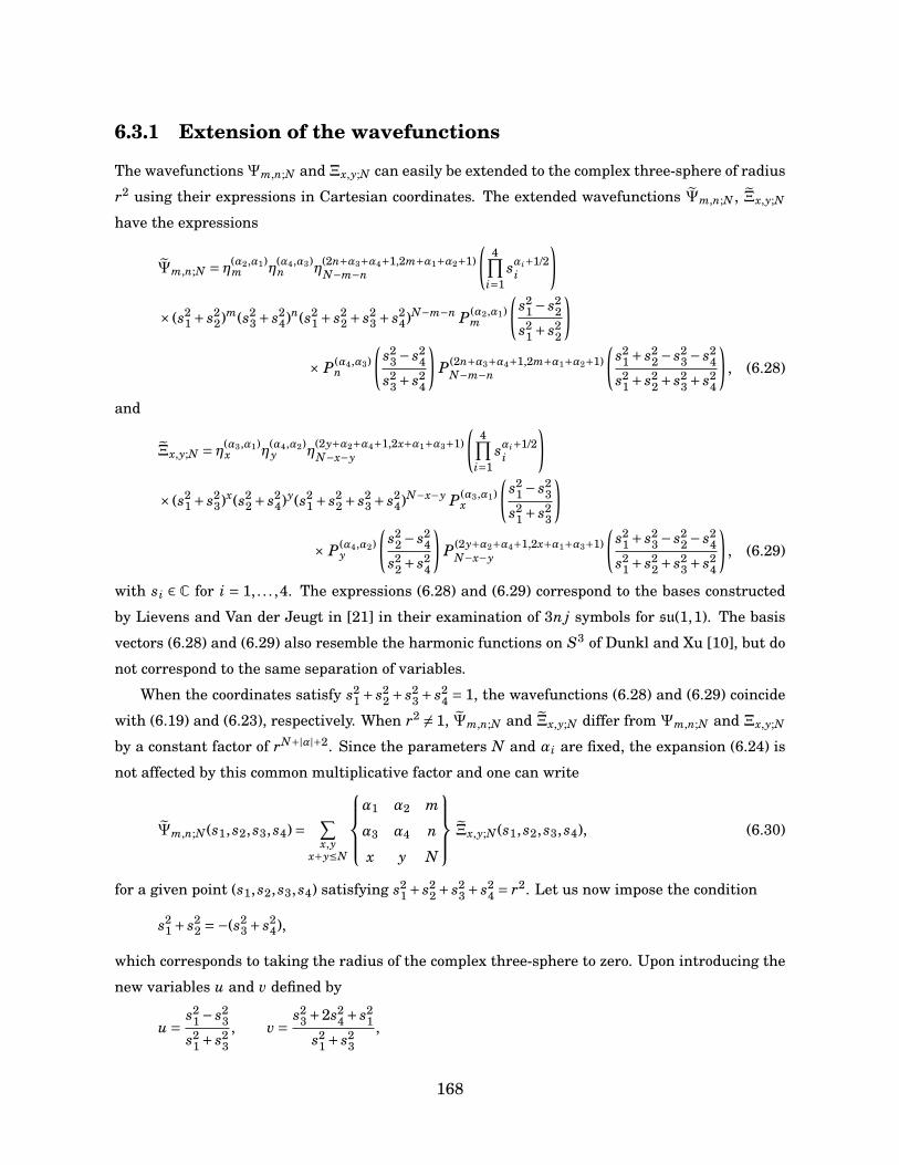
6.3.1 Extension of the wavefunctions
The wavefunctionsΨm,n;N and Ξx,y;N can easily be extended to the complex three-sphere of radius
r2 using their expressions in Cartesian coordinates. The extended wavefunctions Ψm,n;N , Ξx,y;N
have the expressions
Ψm,n;N = η(α2,α1)m η
(α4,α3)n η
(2n+α3+α4+1,2m+α1+α2+1)N−m−n
(4∏
i=1sαi+1/2
i
)
× (s21 + s2
2)m(s23 + s2
4)n(s21 + s2
2 + s23 + s2
4)N−m−n P(α2,α1)m
(s2
1 − s22
s21 + s2
2
)
× P(α4,α3)n
(s2
3 − s24
s23 + s2
4
)P(2n+α3+α4+1,2m+α1+α2+1)
N−m−n
(s2
1 + s22 − s2
3 − s24
s21 + s2
2 + s23 + s2
4
), (6.28)
and
Ξx,y;N = η(α3,α1)x η
(α4,α2)y η
(2y+α2+α4+1,2x+α1+α3+1)N−x−y
(4∏
i=1sαi+1/2
i
)
× (s21 + s2
3)x(s22 + s2
4)y(s21 + s2
2 + s23 + s2
4)N−x−y P(α3,α1)x
(s2
1 − s23
s21 + s2
3
)
× P(α4,α2)y
(s2
2 − s24
s22 + s2
4
)P(2y+α2+α4+1,2x+α1+α3+1)
N−x−y
(s2
1 + s23 − s2
2 − s24
s21 + s2
2 + s23 + s2
4
), (6.29)
with si ∈ C for i = 1, . . . ,4. The expressions (6.28) and (6.29) correspond to the bases constructed
by Lievens and Van der Jeugt in [21] in their examination of 3n j symbols for su(1,1). The basis
vectors (6.28) and (6.29) also resemble the harmonic functions on S3 of Dunkl and Xu [10], but do
not correspond to the same separation of variables.
When the coordinates satisfy s21 + s2
2 + s23 + s2
4 = 1, the wavefunctions (6.28) and (6.29) coincide
with (6.19) and (6.23), respectively. When r2 6= 1, Ψm,n;N and Ξx,y;N differ from Ψm,n;N and Ξx,y;N
by a constant factor of rN+|α|+2. Since the parameters N and αi are fixed, the expansion (6.24) is
not affected by this common multiplicative factor and one can write
Ψm,n;N (s1, s2, s3, s4)= ∑x,y
x+y≤N
α1 α2 m
α3 α4 n
x y N
Ξx,y;N (s1, s2, s3, s4), (6.30)
for a given point (s1, s2, s3, s4) satisfying s21 + s2
2 + s23 + s2
4 = r2. Let us now impose the condition
s21 + s2
2 =−(s23 + s2
4),
which corresponds to taking the radius of the complex three-sphere to zero. Upon introducing the
new variables u and v defined by
u = s21 − s2
3
s21 + s2
3, v = s2
3 +2s24 + s2
1
s21 + s2
3,
168
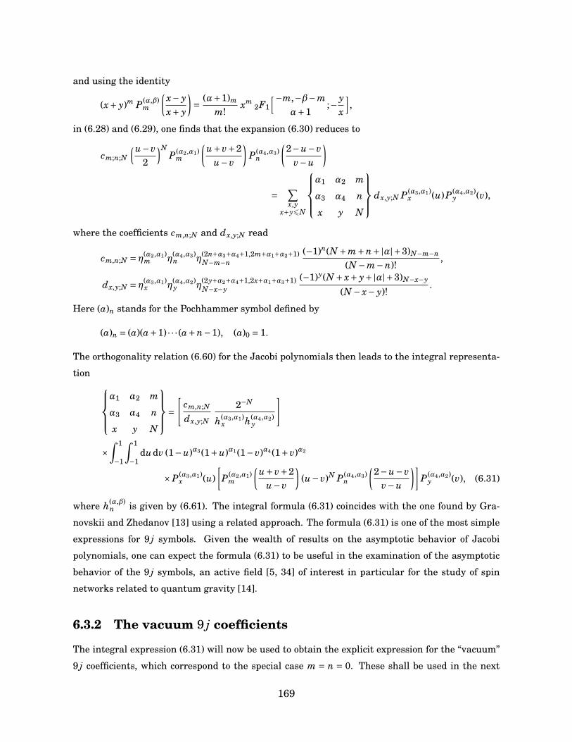
and using the identity
(x+ y)m P(α,β)m
(x− yx+ y
)= (α+1)m
m!xm
2F1
[−m,−β−mα+1
;− yx
],
in (6.28) and (6.29), one finds that the expansion (6.30) reduces to
cm;n;N
(u−v2
)NP(α2,α1)
m
(u+v+2
u−v
)P(α4,α3)
n
(2−u−v
v−u
)
= ∑x,y
x+y6N
α1 α2 m
α3 α4 n
x y N
dx,y;N P(α3,α1)x (u)P(α4,α2)
y (v),
where the coefficients cm,n;N and dx,y;N read
cm,n;N = η(α2,α1)m η
(α4,α3)n η
(2n+α3+α4+1,2m+α1+α2+1)N−m−n
(−1)n(N +m+n+|α|+3)N−m−n
(N −m−n)!,
dx,y;N = η(α3,α1)x η
(α4,α2)y η
(2y+α2+α4+1,2x+α1+α3+1)N−x−y
(−1)y(N + x+ y+|α|+3)N−x−y
(N − x− y)!.
Here (a)n stands for the Pochhammer symbol defined by
(a)n = (a)(a+1) · · · (a+n−1), (a)0 = 1.
The orthogonality relation (6.60) for the Jacobi polynomials then leads to the integral representa-
tion α1 α2 m
α3 α4 n
x y N
=[
cm,n;N
dx,y;N
2−N
h(α3,α1)x h(α4,α2)
y
]
×∫ 1
−1
∫ 1
−1dudv (1−u)α3(1+u)α1(1−v)α4(1+v)α2
×P(α3,α1)x (u)
[P(α2,α1)
m
(u+v+2
u−v
)(u−v)N P(α4,α3)
n
(2−u−v
v−u
)]P(α4,α2)
y (v), (6.31)
where h(α,β)n is given by (6.61). The integral formula (6.31) coincides with the one found by Gra-
novskii and Zhedanov [13] using a related approach. The formula (6.31) is one of the most simple
expressions for 9 j symbols. Given the wealth of results on the asymptotic behavior of Jacobi
polynomials, one can expect the formula (6.31) to be useful in the examination of the asymptotic
behavior of the 9 j symbols, an active field [5, 34] of interest in particular for the study of spin
networks related to quantum gravity [14].
6.3.2 The vacuum 9 j coefficients
The integral expression (6.31) will now be used to obtain the explicit expression for the “vacuum”
9 j coefficients, which correspond to the special case m = n = 0. These shall be used in the next
169
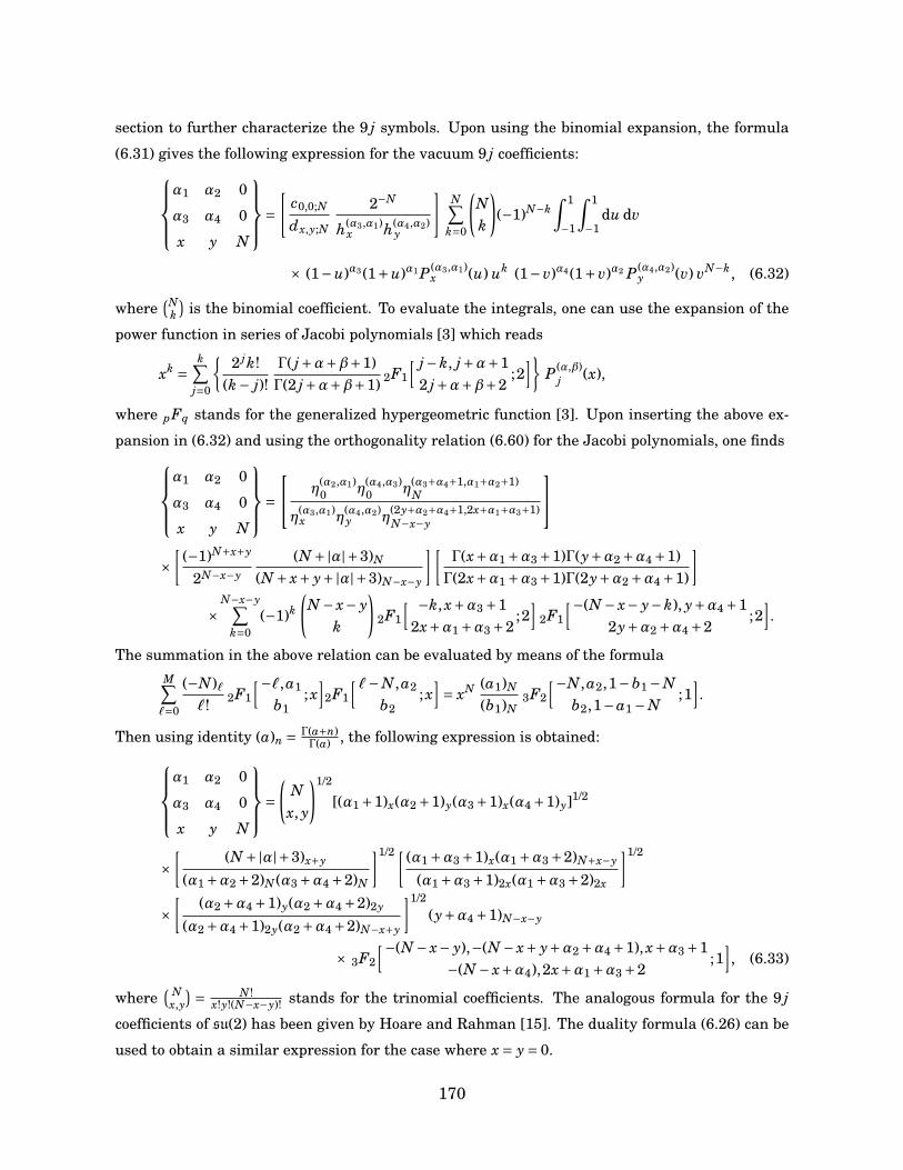
section to further characterize the 9 j symbols. Upon using the binomial expansion, the formula
(6.31) gives the following expression for the vacuum 9 j coefficients:α1 α2 0
α3 α4 0
x y N
=[
c0,0;N
dx,y;N
2−N
h(α3,α1)x h(α4,α2)
y
]N∑
k=0
(Nk
)(−1)N−k
∫ 1
−1
∫ 1
−1du dv
× (1−u)α3(1+u)α1 P(α3,α1)x (u) uk (1− v)α4(1+ v)α2 P(α4,α2)
y (v) vN−k, (6.32)
where(N
k)
is the binomial coefficient. To evaluate the integrals, one can use the expansion of the
power function in series of Jacobi polynomials [3] which reads
xk =k∑
j=0
2 jk!
(k− j)!Γ( j+α+β+1)Γ(2 j+α+β+1) 2F1
[ j−k, j+α+12 j+α+β+2
;2]
P(α,β)j (x),
where pFq stands for the generalized hypergeometric function [3]. Upon inserting the above ex-
pansion in (6.32) and using the orthogonality relation (6.60) for the Jacobi polynomials, one findsα1 α2 0
α3 α4 0
x y N
= η
(α2,α1)0 η
(α4,α3)0 η
(α3+α4+1,α1+α2+1)N
η(α3,α1)x η
(α4,α2)y η
(2y+α2+α4+1,2x+α1+α3+1)N−x−y
×
[(−1)N+x+y
2N−x−y(N +|α|+3)N
(N + x+ y+|α|+3)N−x−y
][Γ(x+α1 +α3 +1)Γ(y+α2 +α4 +1)Γ(2x+α1 +α3 +1)Γ(2y+α2 +α4 +1)
]
×N−x−y∑
k=0(−1)k
(N − x− y
k
)2F1
[ −k, x+α3 +12x+α1 +α3 +2
;2]
2F1
[−(N − x− y−k), y+α4 +12y+α2 +α4 +2
;2].
The summation in the above relation can be evaluated by means of the formulaM∑`=0
(−N)``! 2F1
[−`,a1
b1; x
]2F1
[`−N,a2
b2; x
]= xN (a1)N
(b1)N3F2
[−N,a2,1−b1 −Nb2,1−a1 −N
;1].
Then using identity (a)n = Γ(a+n)Γ(a) , the following expression is obtained:
α1 α2 0
α3 α4 0
x y N
=(
Nx, y
)1/2
[(α1 +1)x(α2 +1)y(α3 +1)x(α4 +1)y]1/2
×[ (N +|α|+3)x+y
(α1 +α2 +2)N (α3 +α4 +2)N
]1/2 [ (α1 +α3 +1)x(α1 +α3 +2)N+x−y
(α1 +α3 +1)2x(α1 +α3 +2)2x
]1/2
×[ (α2 +α4 +1)y(α2 +α4 +2)2y
(α2 +α4 +1)2y(α2 +α4 +2)N−x+y
]1/2(y+α4 +1)N−x−y
× 3F2
[−(N − x− y),−(N − x+ y+α2 +α4 +1), x+α3 +1−(N − x+α4),2x+α1 +α3 +2
;1], (6.33)
where( Nx,y
) = N!x!y!(N−x−y)! stands for the trinomial coefficients. The analogous formula for the 9 j
coefficients of su(2) has been given by Hoare and Rahman [15]. The duality formula (6.26) can be
used to obtain a similar expression for the case where x = y= 0.
170
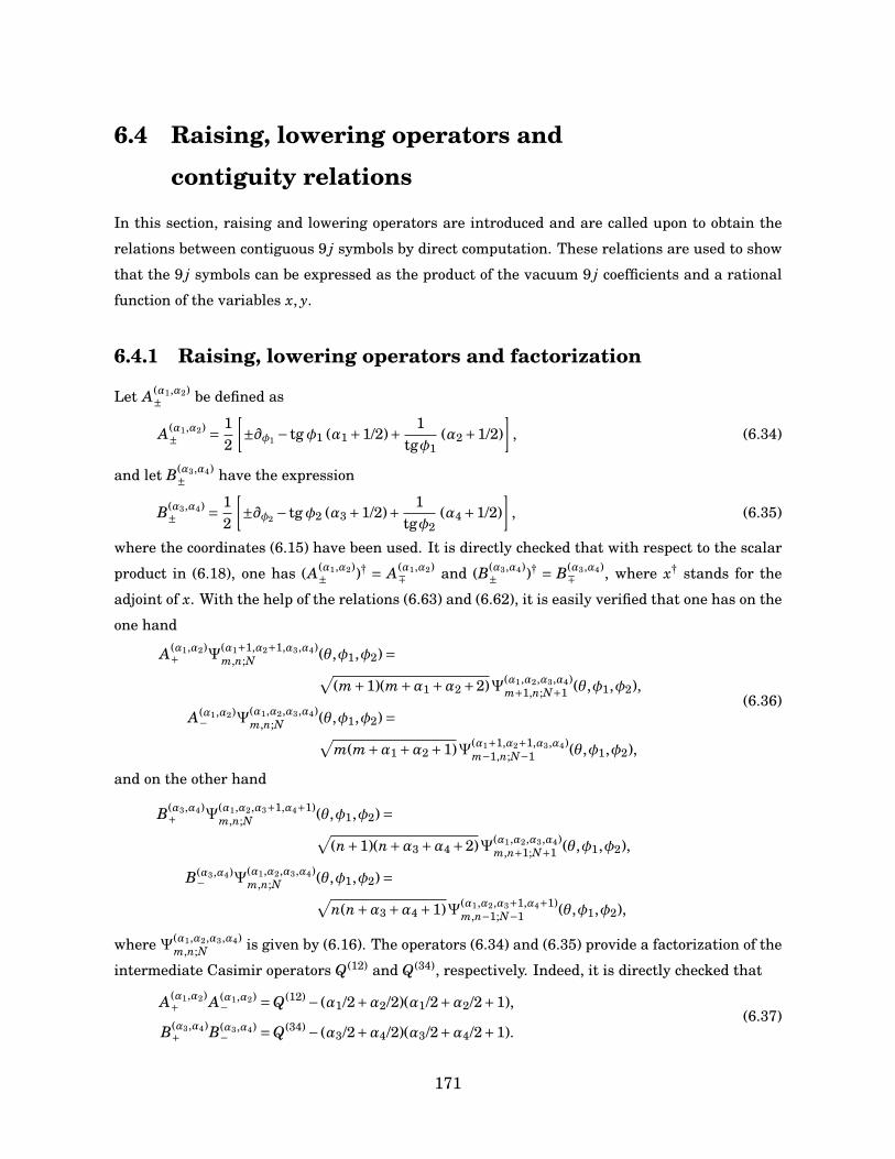
6.4 Raising, lowering operators and
contiguity relations
In this section, raising and lowering operators are introduced and are called upon to obtain the
relations between contiguous 9 j symbols by direct computation. These relations are used to show
that the 9 j symbols can be expressed as the product of the vacuum 9 j coefficients and a rational
function of the variables x, y.
6.4.1 Raising, lowering operators and factorization
Let A(α1,α2)± be defined as
A(α1,α2)± = 1
2
[±∂φ1 − tgφ1 (α1 +1/2)+ 1
tgφ1(α2 +1/2)
], (6.34)
and let B(α3,α4)± have the expression
B(α3,α4)± = 1
2
[±∂φ2 − tgφ2 (α3 +1/2)+ 1
tgφ2(α4 +1/2)
], (6.35)
where the coordinates (6.15) have been used. It is directly checked that with respect to the scalar
product in (6.18), one has (A(α1,α2)± )† = A(α1,α2)
∓ and (B(α3,α4)± )† = B(α3,α4)
∓ , where x† stands for the
adjoint of x. With the help of the relations (6.63) and (6.62), it is easily verified that one has on the
one hand
A(α1,α2)+ Ψ
(α1+1,α2+1,α3,α4)m,n;N (θ,φ1,φ2)=√
(m+1)(m+α1 +α2 +2)Ψ(α1,α2,α3,α4)m+1,n;N+1 (θ,φ1,φ2),
A(α1,α2)− Ψ
(α1,α2,α3,α4)m,n;N (θ,φ1,φ2)=√
m(m+α1 +α2 +1)Ψ(α1+1,α2+1,α3,α4)m−1,n;N−1 (θ,φ1,φ2),
(6.36)
and on the other hand
B(α3,α4)+ Ψ
(α1,α2,α3+1,α4+1)m,n;N (θ,φ1,φ2)=√
(n+1)(n+α3 +α4 +2)Ψ(α1,α2,α3,α4)m,n+1;N+1 (θ,φ1,φ2),
B(α3,α4)− Ψ
(α1,α2,α3,α4)m,n;N (θ,φ1,φ2)=√
n(n+α3 +α4 +1)Ψ(α1,α2,α3+1,α4+1)m,n−1;N−1 (θ,φ1,φ2),
where Ψ(α1,α2,α3,α4)m,n;N is given by (6.16). The operators (6.34) and (6.35) provide a factorization of the
intermediate Casimir operators Q(12) and Q(34), respectively. Indeed, it is directly checked that
A(α1,α2)+ A(α1,α2)
− =Q(12) − (α1/2+α2/2)(α1/2+α2/2+1),
B(α3,α4)+ B(α3,α4)
− =Q(34) − (α3/2+α4/2)(α3/2+α4/2+1).(6.37)
171

6.4.2 Contiguity relations
The raising/lowering operators (6.34) and (6.35) can be used to obtain the relations satisfied by
contiguous 9 j symbols. To facilitate the computations, let us make explicit the dependence of the
canonical basis vectors | m,n ⟩N , | x, y ⟩N on the parameters αi by writing
| m,n ⟩N ≡|α1,α2,α3,α4;m,n ⟩N , | x, y ⟩N ≡|α1,α2,α3,α4; x, y ⟩N .
With this notation the 9 j symbols are written asα1 α2 m
α3 α4 n
x y N
= N⟨α1,α2,α3,α4; x, y |α1,α2,α3,α4;m,n ⟩N .
To obtain the first contiguity relation for 9 j symbols, one considers the matrix element
N⟨α1,α2,α3,α4; x, y | A(α1,α2)+ |α1 +1,α2 +1,α3,α4;m,n ⟩N−1.
By acting with A(α1,α2)+ on |α1 +1,α2 +1,α3,α4;m,n ⟩N−1 using (6.36), one finds
√(m+1)(m+α1 +α2 +2)
α1 α2 m+1
α3 α4 n
x y N
=
N⟨α1,α2,α3,α4; x, y | A(α1,α2)+ |α1 +1,α2 +1,α3,α4;m,n ⟩N−1. (6.38)
To obtain the desired relation, one must determine N⟨α1,α2,α3,α4; x, y |A(α1,α2)+ or equivalently
(A(α1,α2)+ )†|α1,α2,α3,α4; x, y ⟩N = A(α1,α2)
− |α1,α2,α3,α4; x, y ⟩N ,
where the reality of the basis functions Ξx,y;N has been used. This can be done directly by writing
A(α1,α2)− in the coordinates ϑ,ϕ1,ϕ2 defined in (6.20), acting with this operator on the wavefunc-
tions Ξ(α1,α2,α3,α4)x,y;N (ϑ,ϕ1,ϕ2) and using the properties of the Jacobi polynomials. Since this step
represents no fundamental difficulties, the details of the computation are relegated to appendix B.
One finds that
A(α1,α2)− Ξ
(α1,α2,α3,α4)x,y;N =√
(x+α1+1)(x+α13+1)(y+α2+1)(y+α24+1)(N−x−y)(N+x+y+|α|+3)(2x+α13+1)(2x+α13+2)(2y+α24+1)(2y+α24+2) × Ξ
(α1+1,α2+1,α3,α4)x,y;N−1
+√
x(x+α3)(y+α2+1)(y+α24+1)(N−x+y+α24+2)(N+x−y+α13+1)(2x+α13)(2x+α13+1)(2y+α24+1)(2y+α24+2) × Ξ
(α1+1,α2+1,α3,α4)x−1,y;N−1
−√
(x+α1+1)(x+α13+1)y(y+α4)(N+x−y+α13+2)(N−x+y+α24+1)(2x+α13+1)(2x+α13+2)(2y+α24)(2y+α24+1) × Ξ
(α1+1,α2+1,α3,α4)x,y−1;N−1
−√
x(x+α3)y(y+α4)(N−x−y+1)(N+x+y+|α|+2)(2x+α13)(2x+α13+1)(2y+α24)(2y+α24+1) × Ξ
(α1+1,α2+1,α3,α4)x−1,y−1;N−1 , (6.39)
172
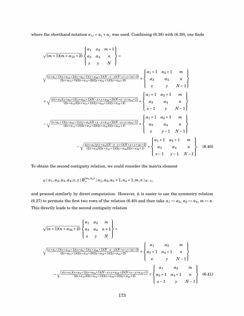
where the shorthand notation αi j =αi +α j was used. Combining (6.38) with (6.39), one finds
√(m+1)(m+α12 +2)
α1 α2 m+1
α3 α4 n
x y N
=
√(x+α1+1)(x+α13+1)(y+α2+1)(y+α24+1)(N−x−y)(N+x+y+|α|+3)
(2x+α13+1)(2x+α13+2)(2y+α24+1)(2y+α24+2) ×
α1 +1 α2 +1 m
α3 α4 n
x y N −1
+
√x(x+α3)(y+α2+1)(y+α24+1)(N−x+y+α24+2)(N+x−y+α13+1)
(2x+α13)(2x+α13+1)(2y+α24+1)(2y+α24+2) ×
α1 +1 α2 +1 m
α3 α4 n
x−1 y N −1
−
√(x+α1+1)(x+α13+1)y(y+α4)(N+x−y+α13+2)(N−x+y+α24+1)
(2x+α13+1)(2x+α13+2)(2y+α24)(2y+α24+1) ×
α1 +1 α2 +1 m
α3 α4 n
x y−1 N −1
−
√x(x+α3)y(y+α4)(N−x−y+1)(N+x+y+|α|+2)
(2x+α13)(2x+α13+1)(2y+α24)(2y+α24+1) ×
α1 +1 α2 +1 m
α3 α4 n
x−1 y−1 N −1
. (6.40)
To obtain the second contiguity relation, we could consider the matrix element
N⟨α1,α2,α3,α4; x, y | B(α3,α4)+ |α1,α2,α3 +1,α4 +1;m,n ⟩N−1,
and proceed similarly by direct computation. However, it is easier to use the symmetry relation
(6.27) to permute the first two rows of the relation (6.40) and then take α1 ↔α3, α2 ↔α4, m ↔ n.
This directly leads to the second contiguity relation
√(n+1)(n+α34 +2)
α1 α2 m
α3 α4 n+1
x y N
=
√(x+α3+1)(x+α13+1)(y+α4+1)(y+α24+1)(N−x−y)(N+x+y+|α|+3)
(2x+α13+1)(2x+α13+2)(2y+α24+1)(2y+α24+2) ×
α1 α2 m
α3 +1 α4 +1 n
x y N −1
−
√x(x+α1)(y+α4+1)(y+α24+1)(N−x+y+α24+2)(N+x−y+α13+1)
(2x+α13)(2x+α13+1)(2y+α24+1)(2y+α24+2) ×
α1 α2 m
α3 +1 α4 +1 n
x−1 y N −1
(6.41)
173
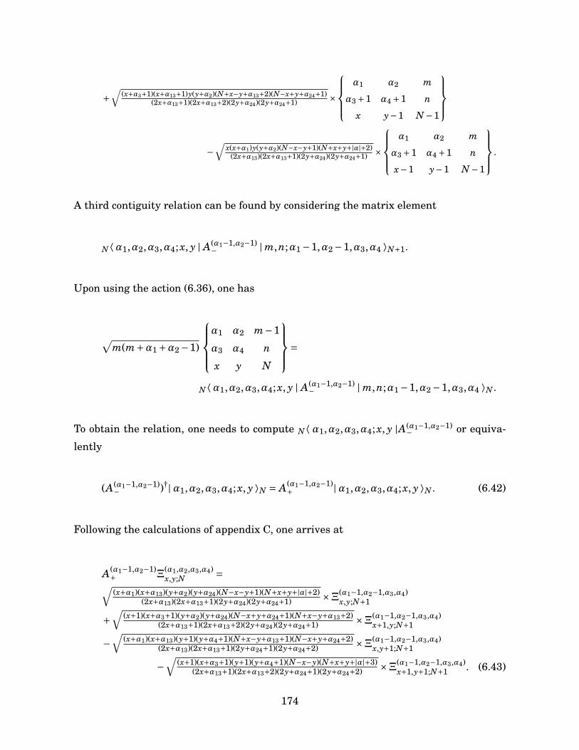
+√
(x+α3+1)(x+α13+1)y(y+α2)(N+x−y+α13+2)(N−x+y+α24+1)(2x+α13+1)(2x+α13+2)(2y+α24)(2y+α24+1) ×
α1 α2 m
α3 +1 α4 +1 n
x y−1 N −1
−
√x(x+α1)y(y+α2)(N−x−y+1)(N+x+y+|α|+2)
(2x+α13)(2x+α13+1)(2y+α24)(2y+α24+1) ×
α1 α2 m
α3 +1 α4 +1 n
x−1 y−1 N −1
.
A third contiguity relation can be found by considering the matrix element
N⟨α1,α2,α3,α4; x, y | A(α1−1,α2−1)− | m,n;α1 −1,α2 −1,α3,α4 ⟩N+1.
Upon using the action (6.36), one has
√m(m+α1 +α2 −1)
α1 α2 m−1
α3 α4 n
x y N
=
N⟨α1,α2,α3,α4; x, y | A(α1−1,α2−1)− | m,n;α1 −1,α2 −1,α3,α4 ⟩N .
To obtain the relation, one needs to compute N⟨ α1,α2,α3,α4; x, y |A(α1−1,α2−1)− or equiva-
lently
(A(α1−1,α2−1)− )†|α1,α2,α3,α4; x, y ⟩N = A(α1−1,α2−1)
+ |α1,α2,α3,α4; x, y ⟩N . (6.42)
Following the calculations of appendix C, one arrives at
A(α1−1,α2−1)+ Ξ
(α1,α2,α3,α4)x,y;N =√
(x+α1)(x+α13)(y+α2)(y+α24)(N−x−y+1)(N+x+y+|α|+2)(2x+α13)(2x+α13+1)(2y+α24)(2y+α24+1) ×Ξ(α1−1,α2−1,α3,α4)
x,y;N+1
+√
(x+1)(x+α3+1)(y+α2)(y+α24)(N−x+y+α24+1)(N+x−y+α13+2)(2x+α13+1)(2x+α13+2)(2y+α24)(2y+α24+1) ×Ξ(α1−1,α2−1,α3,α4)
x+1,y;N+1
−√
(x+α1)(x+α13)(y+1)(y+α4+1)(N+x−y+α13+1)(N−x+y+α24+2)(2x+α13)(2x+α13+1)(2y+α24+1)(2y+α24+2) ×Ξ(α1−1,α2−1,α3,α4)
x,y+1;N+1
−√
(x+1)(x+α3+1)(y+1)(y+α4+1)(N−x−y)(N+x+y+|α|+3)(2x+α13+1)(2x+α13+2)(2y+α24+1)(2y+α24+2) ×Ξ(α1−1,α2−1,α3,α4)
x+1,y+1;N+1 . (6.43)
174
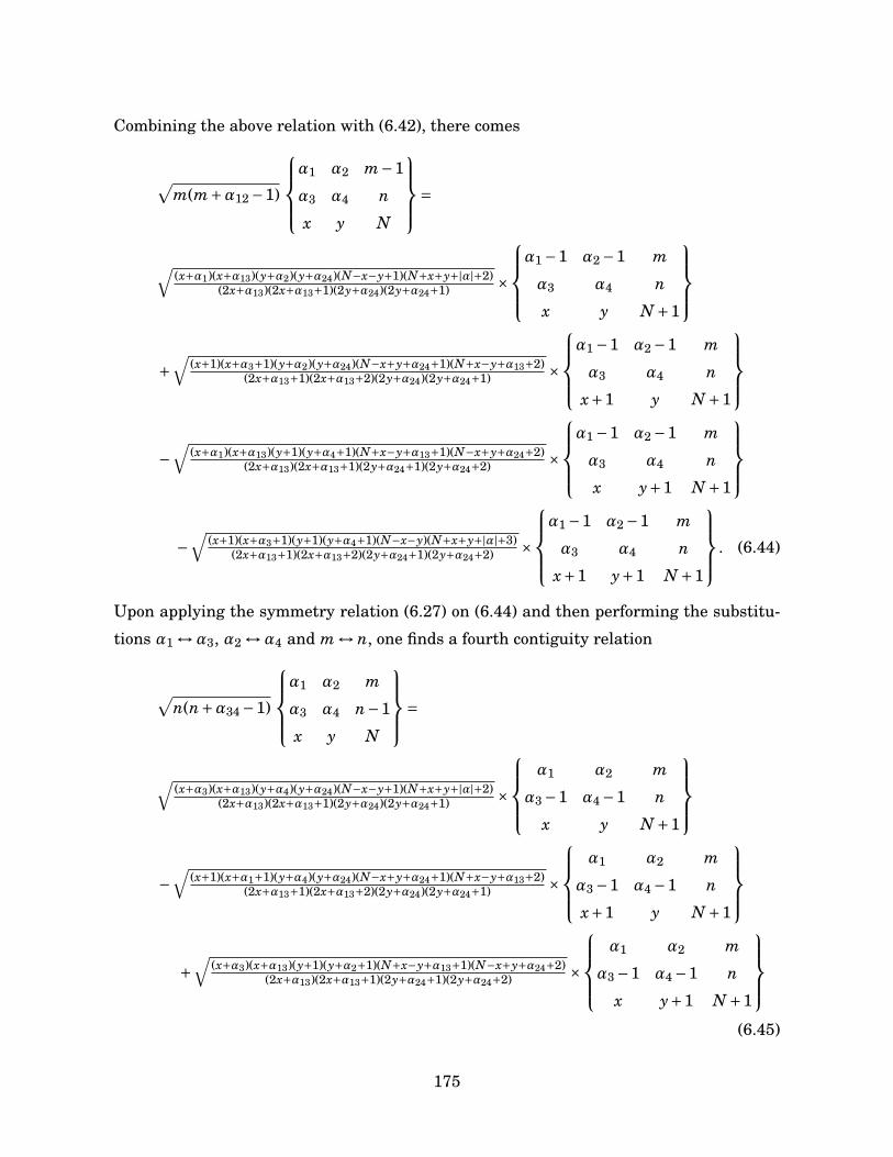
Combining the above relation with (6.42), there comes
√m(m+α12 −1)
α1 α2 m−1
α3 α4 n
x y N
=
√(x+α1)(x+α13)(y+α2)(y+α24)(N−x−y+1)(N+x+y+|α|+2)
(2x+α13)(2x+α13+1)(2y+α24)(2y+α24+1) ×
α1 −1 α2 −1 m
α3 α4 n
x y N +1
+
√(x+1)(x+α3+1)(y+α2)(y+α24)(N−x+y+α24+1)(N+x−y+α13+2)
(2x+α13+1)(2x+α13+2)(2y+α24)(2y+α24+1) ×
α1 −1 α2 −1 m
α3 α4 n
x+1 y N +1
−
√(x+α1)(x+α13)(y+1)(y+α4+1)(N+x−y+α13+1)(N−x+y+α24+2)
(2x+α13)(2x+α13+1)(2y+α24+1)(2y+α24+2) ×
α1 −1 α2 −1 m
α3 α4 n
x y+1 N +1
−
√(x+1)(x+α3+1)(y+1)(y+α4+1)(N−x−y)(N+x+y+|α|+3)
(2x+α13+1)(2x+α13+2)(2y+α24+1)(2y+α24+2) ×
α1 −1 α2 −1 m
α3 α4 n
x+1 y+1 N +1
. (6.44)
Upon applying the symmetry relation (6.27) on (6.44) and then performing the substitu-
tions α1 ↔α3, α2 ↔α4 and m ↔ n, one finds a fourth contiguity relation
√n(n+α34 −1)
α1 α2 m
α3 α4 n−1
x y N
=
√(x+α3)(x+α13)(y+α4)(y+α24)(N−x−y+1)(N+x+y+|α|+2)
(2x+α13)(2x+α13+1)(2y+α24)(2y+α24+1) ×
α1 α2 m
α3 −1 α4 −1 n
x y N +1
−
√(x+1)(x+α1+1)(y+α4)(y+α24)(N−x+y+α24+1)(N+x−y+α13+2)
(2x+α13+1)(2x+α13+2)(2y+α24)(2y+α24+1) ×
α1 α2 m
α3 −1 α4 −1 n
x+1 y N +1
+
√(x+α3)(x+α13)(y+1)(y+α2+1)(N+x−y+α13+1)(N−x+y+α24+2)
(2x+α13)(2x+α13+1)(2y+α24+1)(2y+α24+2) ×
α1 α2 m
α3 −1 α4 −1 n
x y+1 N +1
(6.45)
175
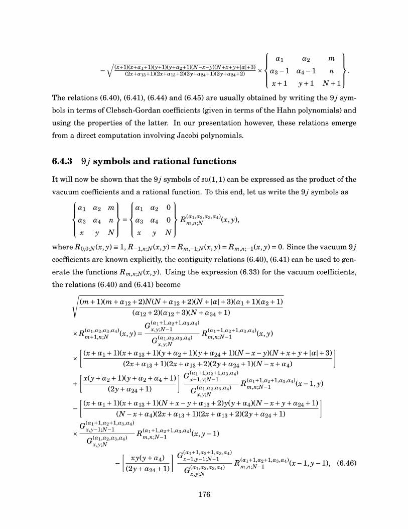
−√
(x+1)(x+α1+1)(y+1)(y+α2+1)(N−x−y)(N+x+y+|α|+3)(2x+α13+1)(2x+α13+2)(2y+α24+1)(2y+α24+2) ×
α1 α2 m
α3 −1 α4 −1 n
x+1 y+1 N +1
.
The relations (6.40), (6.41), (6.44) and (6.45) are usually obtained by writing the 9 j sym-
bols in terms of Clebsch-Gordan coefficients (given in terms of the Hahn polynomials) and
using the properties of the latter. In our presentation however, these relations emerge
from a direct computation involving Jacobi polynomials.
6.4.3 9 j symbols and rational functions
It will now be shown that the 9 j symbols of su(1,1) can be expressed as the product of the
vacuum coefficients and a rational function. To this end, let us write the 9 j symbols asα1 α2 m
α3 α4 n
x y N
=
α1 α2 0
α3 α4 0
x y N
R(α1,α2,α3,α4)m,n;N (x, y),
where R0,0;N(x, y)≡ 1, R−1,n;N(x, y)= Rm,−1;N(x, y)= Rm,n;−1(x, y)= 0. Since the vacuum 9 j
coefficients are known explicitly, the contiguity relations (6.40), (6.41) can be used to gen-
erate the functions Rm,n;N(x, y). Using the expression (6.33) for the vacuum coefficients,
the relations (6.40) and (6.41) become√(m+1)(m+α12 +2)N(N +α12 +2)(N +|α|+3)(α1 +1)(α2 +1)
(α12 +2)(α12 +3)(N +α34 +1)
×R(α1,α2,α3,α4)m+1,n;N (x, y)=
G(α1+1,α2+1,α3,α4)x,y;N−1
G(α1,α2,α3,α4)x,y;N
R(α1+1,α2+1,α3,α4)m,n;N−1 (x, y)
×[
(x+α1 +1)(x+α13 +1)(y+α2 +1)(y+α24 +1)(N − x− y)(N + x+ y+|α|+3)(2x+α13 +1)(2x+α13 +2)(2y+α24 +1)(N − x+α4)
]
+[
x(y+α2 +1)(y+α2 +α4 +1)(2y+α24 +1)
] G(α1+1,α2+1,α3,α4)x−1,y;N−1
G(α1,α2,α3,α4)x,y;N
R(α1+1,α2+1,α3,α4)m,n;N−1 (x−1, y)
−[
(x+α1 +1)(x+α13 +1)(N + x− y+α13 +2)y(y+α4)(N − x+ y+α24 +1)(N − x+α4)(2x+α13 +1)(2x+α13 +2)(2y+α24 +1)
]
×G(α1+1,α2+1,α3,α4)
x,y−1;N−1
G(α1,α2,α3,α4)x,y;N
R(α1+1,α2+1,α3,α4)m,n;N−1 (x, y−1)
−[
xy(y+α4)(2y+α24 +1)
] G(α1+1,α2+1,α3,α4)x−1,y−1;N−1
G(α1,α2,α3,α4)x,y;N
R(α1+1,α2+1,α3,α4)m,n;N−1 (x−1, y−1), (6.46)
176
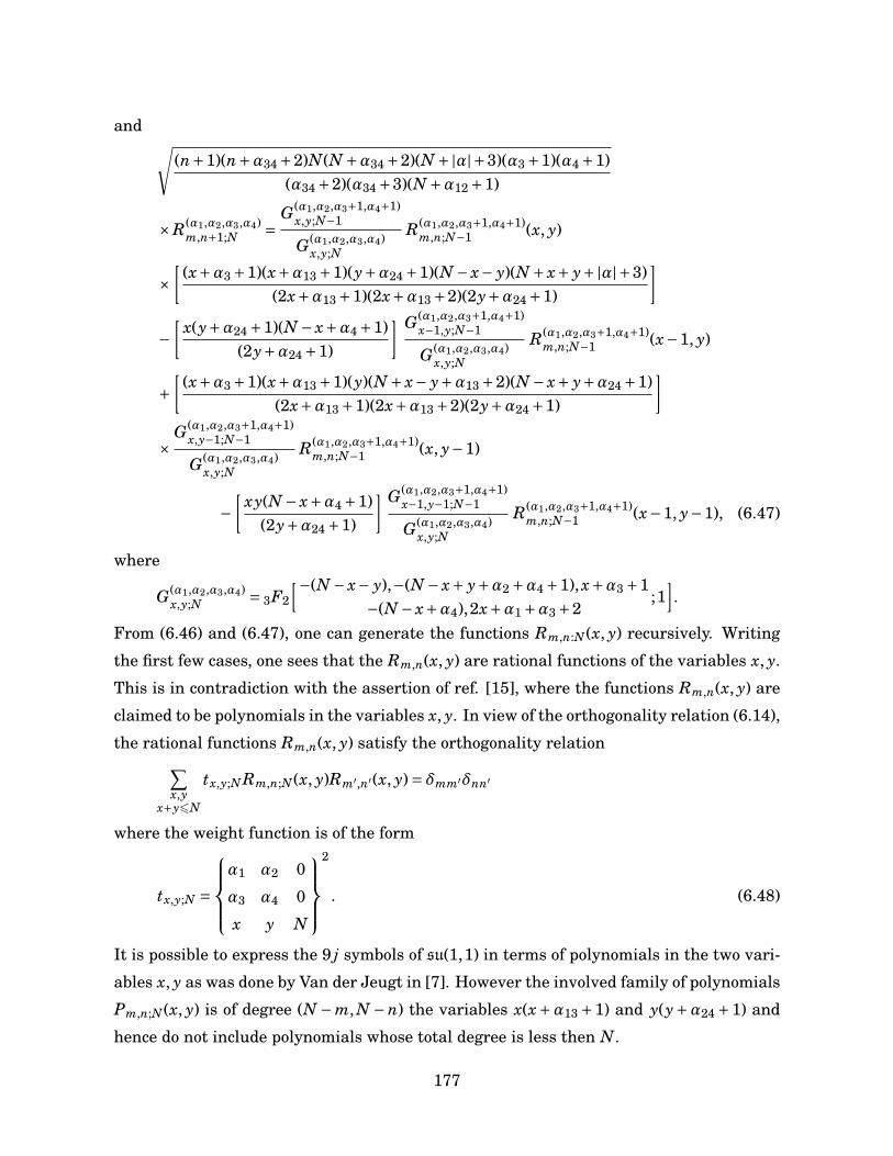
and √(n+1)(n+α34 +2)N(N +α34 +2)(N +|α|+3)(α3 +1)(α4 +1)
(α34 +2)(α34 +3)(N +α12 +1)
×R(α1,α2,α3,α4)m,n+1;N =
G(α1,α2,α3+1,α4+1)x,y;N−1
G(α1,α2,α3,α4)x,y;N
R(α1,α2,α3+1,α4+1)m,n;N−1 (x, y)
×[
(x+α3 +1)(x+α13 +1)(y+α24 +1)(N − x− y)(N + x+ y+|α|+3)(2x+α13 +1)(2x+α13 +2)(2y+α24 +1)
]
−[
x(y+α24 +1)(N − x+α4 +1)(2y+α24 +1)
] G(α1,α2,α3+1,α4+1)x−1,y;N−1
G(α1,α2,α3,α4)x,y;N
R(α1,α2,α3+1,α4+1)m,n;N−1 (x−1, y)
+[
(x+α3 +1)(x+α13 +1)(y)(N + x− y+α13 +2)(N − x+ y+α24 +1)(2x+α13 +1)(2x+α13 +2)(2y+α24 +1)
]
×G(α1,α2,α3+1,α4+1)
x,y−1;N−1
G(α1,α2,α3,α4)x,y;N
R(α1,α2,α3+1,α4+1)m,n;N−1 (x, y−1)
−[
xy(N − x+α4 +1)(2y+α24 +1)
] G(α1,α2,α3+1,α4+1)x−1,y−1;N−1
G(α1,α2,α3,α4)x,y;N
R(α1,α2,α3+1,α4+1)m,n;N−1 (x−1, y−1), (6.47)
where
G(α1,α2,α3,α4)x,y;N = 3F2
[−(N − x− y),−(N − x+ y+α2 +α4 +1), x+α3 +1−(N − x+α4),2x+α1 +α3 +2
;1].
From (6.46) and (6.47), one can generate the functions Rm,n:N(x, y) recursively. Writing
the first few cases, one sees that the Rm,n(x, y) are rational functions of the variables x, y.
This is in contradiction with the assertion of ref. [15], where the functions Rm,n(x, y) are
claimed to be polynomials in the variables x, y. In view of the orthogonality relation (6.14),
the rational functions Rm,n(x, y) satisfy the orthogonality relation∑x,y
x+y6N
tx,y;NRm,n;N(x, y)Rm′,n′(x, y)= δmm′δnn′
where the weight function is of the form
tx,y;N =
α1 α2 0
α3 α4 0
x y N
2
. (6.48)
It is possible to express the 9 j symbols of su(1,1) in terms of polynomials in the two vari-
ables x, y as was done by Van der Jeugt in [7]. However the involved family of polynomials
Pm,n;N(x, y) is of degree (N −m, N − n) the variables x(x+α13 +1) and y(y+α24 +1) and
hence do not include polynomials whose total degree is less then N.
177
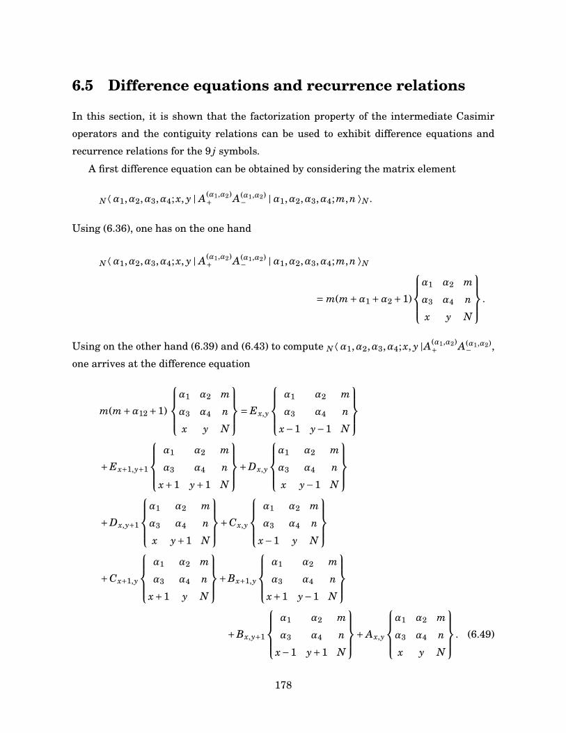
6.5 Difference equations and recurrence relations
In this section, it is shown that the factorization property of the intermediate Casimir
operators and the contiguity relations can be used to exhibit difference equations and
recurrence relations for the 9 j symbols.
A first difference equation can be obtained by considering the matrix element
N⟨α1,α2,α3,α4; x, y | A(α1,α2)+ A(α1,α2)
− |α1,α2,α3,α4;m,n ⟩N .
Using (6.36), one has on the one hand
N⟨α1,α2,α3,α4; x, y | A(α1,α2)+ A(α1,α2)
− |α1,α2,α3,α4;m,n ⟩N
= m(m+α1 +α2 +1)
α1 α2 m
α3 α4 n
x y N
.
Using on the other hand (6.39) and (6.43) to compute N⟨α1,α2,α3,α4; x, y |A(α1,α2)+ A(α1,α2)− ,
one arrives at the difference equation
m(m+α12 +1)
α1 α2 m
α3 α4 n
x y N
= Ex,y
α1 α2 m
α3 α4 n
x−1 y−1 N
+Ex+1,y+1
α1 α2 m
α3 α4 n
x+1 y+1 N
+Dx,y
α1 α2 m
α3 α4 n
x y−1 N
+Dx,y+1
α1 α2 m
α3 α4 n
x y+1 N
+Cx,y
α1 α2 m
α3 α4 n
x−1 y N
+Cx+1,y
α1 α2 m
α3 α4 n
x+1 y N
+Bx+1,y
α1 α2 m
α3 α4 n
x+1 y−1 N
+Bx,y+1
α1 α2 m
α3 α4 n
x−1 y+1 N
+ Ax,y
α1 α2 m
α3 α4 n
x y N
. (6.49)
178
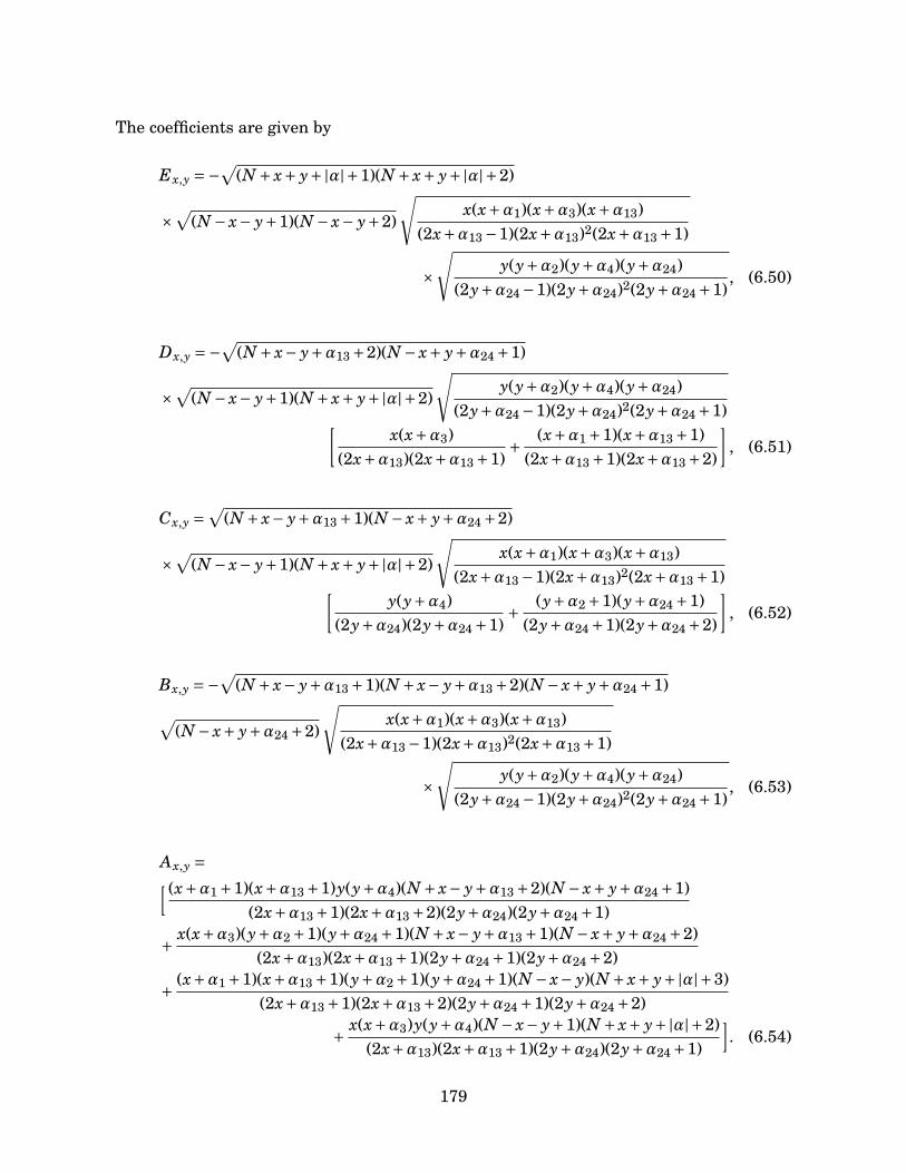
The coefficients are given by
Ex,y =−√(N + x+ y+|α|+1)(N + x+ y+|α|+2)
×√
(N − x− y+1)(N − x− y+2)
√x(x+α1)(x+α3)(x+α13)
(2x+α13 −1)(2x+α13)2(2x+α13 +1)
×√
y(y+α2)(y+α4)(y+α24)(2y+α24 −1)(2y+α24)2(2y+α24 +1)
, (6.50)
Dx,y =−√(N + x− y+α13 +2)(N − x+ y+α24 +1)
×√
(N − x− y+1)(N + x+ y+|α|+2)
√y(y+α2)(y+α4)(y+α24)
(2y+α24 −1)(2y+α24)2(2y+α24 +1)[x(x+α3)
(2x+α13)(2x+α13 +1)+ (x+α1 +1)(x+α13 +1)
(2x+α13 +1)(2x+α13 +2)
], (6.51)
Cx,y =√
(N + x− y+α13 +1)(N − x+ y+α24 +2)
×√
(N − x− y+1)(N + x+ y+|α|+2)
√x(x+α1)(x+α3)(x+α13)
(2x+α13 −1)(2x+α13)2(2x+α13 +1)[y(y+α4)
(2y+α24)(2y+α24 +1)+ (y+α2 +1)(y+α24 +1)
(2y+α24 +1)(2y+α24 +2)
], (6.52)
Bx,y =−√
(N + x− y+α13 +1)(N + x− y+α13 +2)(N − x+ y+α24 +1)
√(N − x+ y+α24 +2)
√x(x+α1)(x+α3)(x+α13)
(2x+α13 −1)(2x+α13)2(2x+α13 +1)
×√
y(y+α2)(y+α4)(y+α24)(2y+α24 −1)(2y+α24)2(2y+α24 +1)
, (6.53)
Ax,y =[ (x+α1 +1)(x+α13 +1)y(y+α4)(N + x− y+α13 +2)(N − x+ y+α24 +1)(2x+α13 +1)(2x+α13 +2)(2y+α24)(2y+α24 +1)
+ x(x+α3)(y+α2 +1)(y+α24 +1)(N + x− y+α13 +1)(N − x+ y+α24 +2)(2x+α13)(2x+α13 +1)(2y+α24 +1)(2y+α24 +2)
+ (x+α1 +1)(x+α13 +1)(y+α2 +1)(y+α24 +1)(N − x− y)(N + x+ y+|α|+3)(2x+α13 +1)(2x+α13 +2)(2y+α24 +1)(2y+α24 +2)
+ x(x+α3)y(y+α4)(N − x− y+1)(N + x+ y+|α|+2)(2x+α13)(2x+α13 +1)(2y+α24)(2y+α24 +1)
]. (6.54)
179
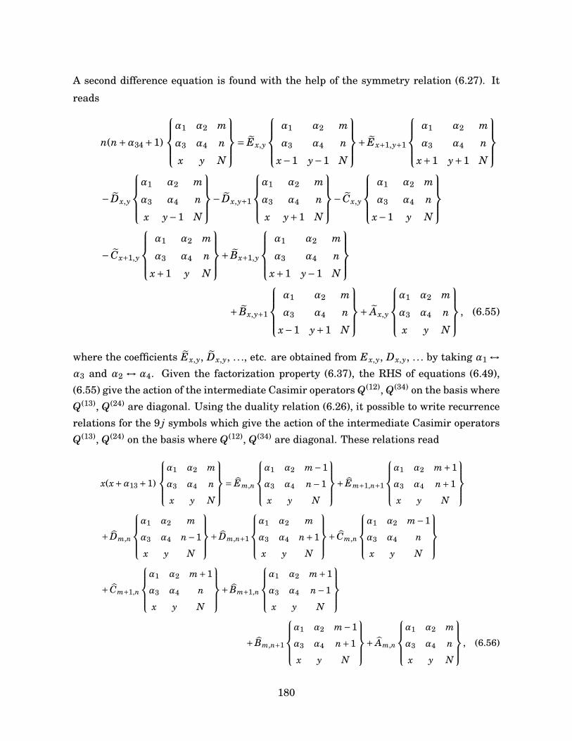
A second difference equation is found with the help of the symmetry relation (6.27). It
reads
n(n+α34 +1)
α1 α2 m
α3 α4 n
x y N
= Ex,y
α1 α2 m
α3 α4 n
x−1 y−1 N
+ Ex+1,y+1
α1 α2 m
α3 α4 n
x+1 y+1 N
− Dx,y
α1 α2 m
α3 α4 n
x y−1 N
− Dx,y+1
α1 α2 m
α3 α4 n
x y+1 N
− Cx,y
α1 α2 m
α3 α4 n
x−1 y N
− Cx+1,y
α1 α2 m
α3 α4 n
x+1 y N
+ Bx+1,y
α1 α2 m
α3 α4 n
x+1 y−1 N
+ Bx,y+1
α1 α2 m
α3 α4 n
x−1 y+1 N
+ Ax,y
α1 α2 m
α3 α4 n
x y N
, (6.55)
where the coefficients Ex,y, Dx,y, . . ., etc. are obtained from Ex,y, Dx,y, . . . by taking α1 ↔α3 and α2 ↔ α4. Given the factorization property (6.37), the RHS of equations (6.49),(6.55) give the action of the intermediate Casimir operators Q(12), Q(34) on the basis whereQ(13), Q(24) are diagonal. Using the duality relation (6.26), it possible to write recurrencerelations for the 9 j symbols which give the action of the intermediate Casimir operatorsQ(13), Q(24) on the basis where Q(12), Q(34) are diagonal. These relations read
x(x+α13 +1)
α1 α2 m
α3 α4 n
x y N
= Em,n
α1 α2 m−1
α3 α4 n−1
x y N
+ Em+1,n+1
α1 α2 m+1
α3 α4 n+1
x y N
+ Dm,n
α1 α2 m
α3 α4 n−1
x y N
+ Dm,n+1
α1 α2 m
α3 α4 n+1
x y N
+ Cm,n
α1 α2 m−1
α3 α4 n
x y N
+ Cm+1,n
α1 α2 m+1
α3 α4 n
x y N
+ Bm+1,n
α1 α2 m+1
α3 α4 n−1
x y N
+ Bm,n+1
α1 α2 m−1
α3 α4 n+1
x y N
+ Am,n
α1 α2 m
α3 α4 n
x y N
, (6.56)
180
where Em,n, Dm,n, . . . are obtained from Em,n, Dm,n, . . . by taking α2 ↔ α3. The secondrecurrence relation is
y(y+α24 +1)
α1 α2 m
α3 α4 n
x y N
= Em,n
α1 α2 m−1
α3 α4 n−1
x y N
+ Em+1,n+1
α1 α2 m+1
α3 α4 n+1
x y N
− Dm,n
α1 α2 m
α3 α4 n−1
x y N
− Dm,n+1
α1 α2 m
α3 α4 n+1
x y N
− Cm,n
α1 α2 m−1
α3 α4 n
x y N
− Cm+1,n
α1 α2 m+1
α3 α4 n
x y N
+ Bm+1,n
α1 α2 m+1
α3 α4 n−1
x y N
+ Bm,n+1
α1 α2 m−1
α3 α4 n+1
x y N
+ Am,n
α1 α2 m
α3 α4 n
x y N
, (6.57)
where Em,n, Dm,n, etc. are obtained from Em,n, Dm,n, etc, by effecting the permutation
σ= (1243) on the parameters (α1,α2,α3,α4). Writing once again the 9 j symbols asα1 α2 m
α3 α4 n
x y N
=
α1 α2 0
α3 α4 0
x y N
Rm,n(x, y),
and defining
R0(x, y)=(1), R1(x, y) =
(R1,0(x, y)
R0,1(x, y)
), R2(x, y)=
R2,0(x, y)
R1,1(x, y)
R0,2(x, y)
, · · ·
the recurrence relations (6.56) and (6.57) can be written in matrix form as follows
x(x+α13 +1)Rn(x, y)= q(1)n+2 Rn+2(x, y)+ r(1)
n+1 Rn+1(x, y)
+ s(1)n Rn(x, y)+ r(1)
n Rn−1(x, y)+ q(1)n Rn−2(x, y), (6.58)
y(y+α24 +1)Rn(x, y)= q(2)n+2 Rn+2(x, y)+ r(2)
n+1 Rn+1(x, y)
+ s(2)n Rn(x, y)+ r(2)
n Rn−1(x, y)+ q(2)n Rn−2(x, y), (6.59)
where the matrices q(i)n , r(i)
n and s(i)n are easily found from the coefficients in (6.56) and
(6.57). It is apparent from (6.58) and (6.59) that the vector functions Rm(x, y) satisfy a five
181
term recurrence relation. In view of the multivariate extension of Favard’s theorem [10],
this confirms that the functions Rm(x, y) are not orthogonal polynomials.
6.6 Conclusion
In this paper, we have used the connection between the addition of four su(1,1) repre-
sentations of the positive discrete series and the generic superintegrable model on the
3-sphere to study the 9 j coefficients in the position representation. We constructed the
canonical basis vectors of the 9 j problem explicitly and related them to the separation of
variables in cylindrical coordinates. Moreover, we have obtained by direct computation
the contiguity relations, the difference equations and the recurrence relations satisfied by
the 9 j symbols. The properties of the 9 j coefficients as bivariate functions have thus been
clarified.
The present work suggests many avenues for further investigations. For example
Lievens and Van der Jeugt [21] have constructed explicitly the coupled basis vectors aris-
ing in the tensor product of an arbitrary number of su(1,1) representations in the coherent
state representation. Given this result, it would be of interest to give the realization of
these vectors in the position representation by examining the generic superintegrable sys-
tem on the n-sphere. Another interesting question is that of the orthogonal polynomials
in two variables connected with the 9 j problem. With the observations of the present
work and those made by Van der Jeugt in ref [6], one must conclude that the study of 9 j
symbols do not naturally lead to families of bivariate orthogonal polynomials that would
be two-variable extensions of the Racah polynomials. However, the results obtained by
Kalnins, Miller and Post [18] and the connection between the generic model on the three-
sphere and the 9 j problem exhibited here suggest that an algebraic interpretation for the
bivariate extension of the Racah polynomials, as defined by Tratnik [32], could be given
in the framework of the addition of four su(1,1) algebras by investigating the overlap co-
efficients between bases which are different from the canonical ones. We plan to follow up
on this.
182
6.A Properties of Jacobi polynomials
The Jacobi polynomials, denoted by P (α,β)n (z), are defined as follows [19]:
P (α,β)n (z)= (α+1)n
n! 2F1
[−n,n+α+β+1α+1
;1− z
2
],
where pFq stands for the generalized hypergeometric function [3]. The polynomials sat-
isfy ∫ 1
−1(1− z)α(1+ z)βP (α,β)
n (z)P (α,β)m (z) dz = h(α,β)
n δnm, (6.60)
where the normalization coefficient is
h(α,β)n = 2α+β+1Γ(2n+α+β+1)Γ(n+α+1)Γ(n+β+1)
Γ(2n+α+β+2)Γ(n+α+β+1)Γ(n+1). (6.61)
The derivatives of the Jacobi polynomials give [23]
∂zP (α,β)n (z)=
[n+α+β+1
2
]P (α+1,β+1)
n−1 (z), (6.62)
∂z
((1− z)α(1+ z)βP (α,β)
n (z))=−2(n+1) (1− z)α−1(1+ z)β−1 P (α−1,β−1)
n+1 (z). (6.63)
One has
P (α,β)n (z)=
(n+α+β+1
2n+α+β+1
)P (α,β+1)
n (z)+(
n+α2n+α+β+1
)P (α,β+1)
n−1 (z). (6.64)
and (1− z
2
)P (α,β)
n−1 (z)= (n+α−1
2n+α+β−1
)P (α1−1,β)
n−1 (z)−(
n2n+α+β−1
)P (α−1,β)
n (z). (6.65)
Since P (α,β)n (−z)= (−1)nP (β,α)
n (z), one has also(1+ z
2
)P (α,β)
n (z)= (n+β
2n+α+β+1
)P (α,β−1)
n (z)+(
n+12n+α+β+1
)P (α,β−1)
n+1 (z), (6.66)
and
P (α,β)n (z)=
(n+α+β+1
2n+α+β+1
)P (α+1,β)
n (z)−(
n+β2n+α+β+1
)P (α+1,β)
n−1 (z). (6.67)
183
6.B Action of A(α1,α2)− on Ξ(α1,α2,α3,α4)
x,y;N
In Cartesian coordinates, the operator A(α1,α2)− reads
A(α1,α2)− =−1
2(s1∂s2 − s2∂s1)+ s1
2s2(α2 +1/2)− s2
2s1(α1 +1/2).
The action of A(α1,α2)− on the wavefunctions Ξ(α1,α2,α3,α4)x,y;N can be written as
F η(α3,α1)x η
(α4,α2)y η
(2y+α24+1,2x+α13+1)N−x−y
×[F−1A(α1,α2)
− F][
P (2y+α24+1,2x+α13+1)N−x−y (cos2ϑ)P (α3,α1)
x(cos2ϕ1
)P (α4,α2)
y(cos2ϕ2
)],
where
F = (s21 + s2
3)x(s22 + s2
4)y4∏
i=1sαi+1/2
i
One has
[F−1A(α1,α2)− F ]=−1
2(s1∂s2 − s2∂s1)+ x
s1s2
s21 + s2
3− y
s1s2
s22 + s2
4.
In the cylindrical coordinates (6.20), the operator reads
[F−1A(α1,α2)− F ]= x
[tgϑcosϕ1 cosϕ2
]− y[
cosϕ1 cosϕ2
tgϑ
]− 1
2
[cosϕ1 cosϕ2∂ϑ+ tgϑsinϕ1 cosϕ2∂ϕ1 −
cosϕ1 sinϕ2
tgϑ∂ϕ2
].
Using the relation (6.62), one finds
A(α1,α2)− Ξ
(α1,α2,α3,α4)x,y;N = υ(α1,α2,α3)
x,y,N
[(N + x+ y+|α|+3)(cos2ϑ)x(sin2ϑ)y
×P (2y+α24+2,2x+α13+2)N−x−y−1 (cos2ϑ)P (α3,α1)
x (cos2ϕ1)P (α4,α2)y (cos2ϕ2)
+ (x+α13 +1)(cos2ϑ)x−1(sin2ϑ)y sin2ϕ1
×P (2y+α24+1,2x+α13+1)N−x−y (cos2ϑ)P (α3+1,α1+1)
x−1 (cos2ϕ1)P (α4,α2)y (cos2ϕ2)
− (y+α24 +1)(cos2ϑ)x(sin2ϑ)y−1 sin2ϕ2
×P (2y+α24+1,2x+α13+1)N−x−y (cos2ϑ)P (α3,α1)
x (cos2ϕ1)P (α4+1,α2+1)y−1 (cos2ϕ2)
+[x(cos2ϑ)x−1(sin2ϑ)y − y(cos2ϑ)x(sin2ϑ)y−1
]×P (2y+α24+1,2x+α13+1)
N−x−y (cos2ϑ)P (α3,α1)x (cos2ϕ1)P (α4,α2)
y (cos2ϕ2)],
184
where
υ(α1,α2,α3)x,y,N = η(α3,α1)
x η(α4,α2)y η
(2y+α24+1,2x+α13+1)N−x−y (s1)α1+3/2(s2)α2+3/2(s3)α3+1/2(s4)α4+1/2.
The identities (6.64) and (6.65) can then be used to write the result in a form involving
only terms of the type P (α3,α1+1)k and P (α4,α2+1)
k′ . Regrouping the terms, one finds
A(α1,α2)− Ξ
(α1,α2,α3,α4)x,y;N = υ(α1,α2,α3)
x,y,N
[(x+α13 +1)(y+α24 +1)(N + x+ y+|α|+3)
(2x+α13 +1)(2y+α24 +1)
×(cos2ϑ)x(sin2ϑ)yP (α3,α1+1)
x (cos2ϕ1)P (α4,α2+1)y (cos2ϕ2)P (2y+α24+2,2x+α13+2)
N−x−y−1 (cos2ϑ)
+
(x+α3)(y+α24 +1)(cos2ϑ)x−1(sin2ϑ)y
(2x+α13 +1)(2y+α24 +1)
P (α3,α1+1)
x−1 (cos2ϕ1)P (α4,α2+1)y (cos2ϕ2)
×((N + x+ y+|α|+3) cos2ϑ P (2y+α24+2,2x+α13+2)
N−x−y−1 (cos2ϑ)
+(2x+α13 +1)P (2y+α24+1,2x+α13+1)N−x−y (cos2ϑ)
)+
(y+α4)(x+α13 +1)(cos2ϑ)x(sin2ϑ)y−1
(2x+α13 +1)(2y+α24 +1)
P (α3,α1+1)
x (cos2ϕ1)P (α4,α2+1)y−1 (cos2ϕ2)
×((N + x+ y+|α|+3) sin2ϑ P (2y+α24+2,2x+α13+2)
N−x−y−1 (cos2ϑ)
−(2y+α24 +1)P (2y+α24+1,2x+α13+1)n−x−y (cos2ϑ)
)+
(y+α4)(x+α3)(cos2ϑ)x−1(sin2ϑ)y−1
(2x+α13 +1)(2y+α24 +1)
P (α3,α1+1)
x−1 (cos2ϕ1)P (α4,α2+1)y−1 (cos2ϕ2)
×((N + x+ y+|α|+3)cos2ϑsin2ϑP (2y+α24+2,2x+α13+2)
N−x−y−1 (cos2ϑ)
+(2x+α13 +1)sin2ϑP (2y+α24+1,2x+α13+1)N−x−y (cos2ϑ)
−(2y+α24 +1)cos2ϑ P (2y+α24+1,2x+α13+1)N−x−y (cos2ϑ)
)]The terms between parentheses in the above expression are easily evaluated and found
to be
(N + x+ y+|α|+3) cos2ϑ P (2y+α24+2,2x+α13+2)N−x−y−1 (cos2ϑ)
+ (2x+α13 +1)P (2y+α24+1,2x+α13+1)N−x−y (cos2ϑ)
= (N + x− y+α13 +1)P (2y+α24+2,2x+α13)N−x−y (cos2ϑ),
(N + x+ y+|α|+3) sin2ϑ P (2y+α24+2,2x+α13+2)N−x−y−1 (cos2ϑ)
− (2y+α24 +1)P (2y+α24+1,2x+α13+1)n−x−y (cos2ϑ)
=−(N − x+ y+α24 +1)P (2y+α24,2x+α13+2)N−x−y (cos2ϑ),
185
(N + x+ y+|α|+3)cos2ϑsin2ϑP (2y+α24+2,2x+α13+2)N−x−y−1 (cos2ϑ)
+ (2x+α13 +1)sin2ϑP (2y+α24+1,2x+α13+1)N−x−y (cos2ϑ)
− (2y+α24 +1)cos2ϑ P (2y+α24+1,2x+α13+1)N−x−y (cos2ϑ)
=−(N − x− y+1)P (2y+α24,2x+α13)N−x−y+1 (cos2ϑ).
Adjusting the normalization factors then yields the result (6.39).
6.C Action of A(α1−1,α2−1)+ on Ξ(α1,α2,α3,α4)
x,y;N
In Cartesian coordinates, the operator A(α1−1,α2−1)+ reads
A(α1−1,α2−1)+ = 1
2(s1∂s2 − s2∂s1)+ s1
2s2(α2 −1/2)− s2
2s1(α1 −1/2).
The action of A(α1−1,α2−1)+ on the wavefunctions Ξx,y;N can be expressed as
G−1η(α3,α1)x η
(α4,α2)y η
(2y+α24+1,2x+α13+1)N−x−y
×[G A(α1−1,α2−1)
+ G−1][
(sin2ϕ1)α3(cos2ϕ1)α1 P (α3,α1)x (cos2ϕ1)
]×
[(sin2ϕ2)α4(cos2ϕ2)α2 P (α4,α2)
y (cos2ϕ2)]
×[(sin2ϑ)2x+α24+1(cos2ϑ)2x+α13+1P (2y+α24+1,2x+α13+1)
N−x−y (cos2ϑ)]
,
where
G = (s21 + s2
3)x+1(s22 + s2
4)y+14∏
i=1sαi−1/2
i .
One has
[G A(α1−1,α2−1)+ G−1]= 1
2(s2∂s1 − s1∂s2)+ (x+1)
s1s2
s21 + s2
3− (y+1)
s1s2
s22 + s2
4.
In the cylindrical coordinates (6.20), this operator reads
[G A(α1−1,α2−1)+ G−1]= 1
2
[cosϕ1 cosϕ2 ∂ϑ+ tgϑsinϕ1 cosϕ2 ∂ϕ1
− cosϕ1 sinϕ2
tgϑ∂ϕ2
]+ (x+1)[tgϑcosϕ1 cosϕ2]− (y+1) [ctgϑcosϕ1 cosϕ2].
186

Using the identity (6.63), one finds
A(α1−1,α2−1)+ Ξ
(α1,α2,α3,α4)x,y;N = κ(α1,α2,α3)
x,y;N
[(N − x− y+1)cos2ϕ1 cos2ϕ2
× (cos2ϑ)x(sin2ϑ)yP (α3,α1)x (cos2ϕ1)P (α4,α2)
y (cos2ϕ2)P (2y+α24,2x+α13)N−x−y+1 (cos2ϑ)
+ (x+1)cos2ϕ2(cos2ϑ)x(sin2ϑ)y+1
×P (α3−1,α1−1)x+1 (cos2ϕ1)P (α4,α2)
y (cos2ϕ2)P (2y+α24+1,2x+α13+1)N−x−y (cos2ϑ)
− (y+1)cos2ϕ1(cos2ϑ)x+1(sin2ϑ)y
×P (α3,α1)x (cos2ϕ1)P (α4−1,α2−1)
y+1 (cos2ϕ2)P (2y+α24+1,2x+α13+1)N−x−y (cos2ϑ)
+ (x+1)cos2ϕ1 cos2ϕ2(cos2ϑ)x(sin2ϑ)y+1
×P (α3,α1)x (cos2ϕ1)P (α4,α2)
y (cos2ϕ2)P (2y+α24+1,2x+α13+1)N−x−y (cos2ϑ)
− (y+1)cos2ϕ1 cos2ϕ2(cos2ϑ)x+1(sin2ϑ)y
×P (α3,α1)x (cos2ϕ1)P (α4,α2)
y (cos2ϕ2)P (2y+α24+1,2x+α13+1)N−x−y (cos2ϑ)
],
where
κ(α1,α2,α3)x,y;N = η(α3,α1)
x η(α4,α2)y η
(2y+α24+1,2x+α13+1)N−x−y (s1)α1−1/2(s2)α2−1/2(s3)α3+1/2(s4)α4+1/2.
Then using (6.66) and (6.67), one finds
A(α1−1,α2−1)+ Ξ
(α1,α2,α3,α4)x,y;N = κ(α1,α2,α3)
x,y;N
[(x+α1)(y+α2)(N − x− y+1)
(2x+α13 +1)(2y+α24 +1)
× (cos2ϑ)x(sin2ϑ)yP (α3,α1−1)
x (cos2ϕ1)P (α4,α2−1)y (cos2ϕ2)P (2y+α24,2x+α13)
N−x−y+1 (cos2ϑ)
+
(x+1)(y+α2)(cos2ϑ)x+1(sin2ϑ)y
(2x+α13 +1)(2y+α24 +1)
P (α3,α1−1)
x+1 (cos2ϕ1)P (α4,α2−1)y (cos2ϕ2)
×([2x+α13 +1]
sin2ϑ
cos2ϑP (2y+α24+1,2x+α13+1)
N−x−y (cos2ϑ)
+ [N − x− y+1]1
cos2ϑP (2y+α24,2x+α13)
N−x−y+1 (cos2ϑ))
+
(x+α1)(y+1)(cos2ϑ)x(sin2ϑ)y+1
(2x+α13 +1)(2y+α24 +1)
P (α3,α1−1)
x (cos2ϕ1)P (α4,α2−1)y+1 (cos2ϕ2)
×([N − x− y+1]
1sin2ϑ
P (2y+α24,2x+α13)N−x−y+1 (cos2ϑ)
187
− [2y+α24 +1]cos2ϑ
sin2ϑP2y+α24+1,2x+α13+1)
N−x−y (cos2ϑ))
+
(x+1)(y+1)(cos2ϑ)x+1(sin2ϑ)y+1
(2x+α13 +1)(2y+α24 +1)
P (α3,α1)
x+1 (cos2ϕ1)P (α4,α−2−1)y+1 (cos2ϕ2)
×([N − x− y+1]
1cos2ϑsin2ϑ
P (2y+α24,2x+α13)N−x−y+1 (cos2ϑ)
− [2y+α24 +1]1
sin2ϑP (2y+α24+1,2x+α13+1)
N−x−y (cos2ϑ)
+ [2x+α13 +1]1
cos2ϑP (2y+α24+1,2x+α13+1)
N−x−y (cos2ϑ)).
The term between the parentheses are easily determined to be the following
[2x+α13 +1]sin2ϑ
cos2ϑP (2y+α24+1,2x+α13+1)
N−x−y (cos2ϑ)
+ [N − x− y+1]1
cos2ϑP (2y+α24,2x+α13)
N−x−y+1 (cos2ϑ)
= (N − x+ y+α24 +1)P (2y+α24,2x+α13+2)N−x−y (cos2ϑ)
[N − x− y+1]1
sin2ϑP (2y+α24,2x+α13)
N−x−y+1 (cos2ϑ)
− [2y+α24 +1]cos2ϑ
sin2ϑP2y+α24+1,2x+α13+1)
N−x−y (cos2ϑ)
=−(N + x− y+α13 +1)P (2y+α24+2,2x+α13)N−x−y (cos2ϑ)
[N − x− y+1]1
cos2ϑsin2ϑP (2y+α24,2x+α13)
N−x−y+1 (cos2ϑ)
− [2y+α24 +1]1
sin2ϑP (2y+α24+1,2x+α13+1)
N−x−y (cos2ϑ)
+ [2x+α13 +1]1
cos2ϑP (2y+α24+1,2x+α13+1)
N−x−y (cos2ϑ)
=−(N + x+ y+|α|+3)P (2y+α24+2,2x+α13+2)N−x−y−1 (cos2ϑ).
Adjusting the normalization factors then yields the result (6.43).
References
[1] Ališauskas S., The Triple Sum Formulas for 9 j coefficients of SU(2) and uq(2), J. Math. Phys.
41 (2000), 7589–7610.
188
[2] Ališauskas S., Jucys A.P., Weight lowering operators and the multiplicity-free isoscalar fac-
tors for the group R5, J. Math. Phys. 12 (1971), 594–605.
[3] Andrews G., Askey R., Roy R., Special functions (1999),.
[4] Arfken G.B., Weber H., Harris F.E., Mathematical Methods for Physicists, 7th ed., Academic
Press, 2012.
[5] Bonzom V., Fleury P., Asymptotics of Wigner 3n j -symbols with small and large angular
momenta: an elementary method, J. Phys. A: Math. Theor. 45 (2012), 075202.
[6] Van der Jeugt J., Coupling coefficients for Lie algebra representations and addition formulas
for special functions, J. Math. Phys. 38 (1997), 2728.
[7] Van der Jeugt J., Hypergeometric series related to the 9− j coefficient of su(1,1), J. Comp.
Appl. Math. 118 (2000), 337–351.
[8] Van der Jeugt J., 3n j-Coefficients and Orthogonal Polynomials of Hypergeometric Type, in
Orthogonal Polynomials and Special Functions, Editors E. Koelink, W.V. Assche, Lecture
Notes in Mathematics Vol. 1817, Springer, 2003.
[9] Diaconis P., Griffiths R.C., An introduction to multivariate Krawtchouk polynomials and
their applications, J. Stat. Plann. Inf. (2014),.
[10] Dunkl C.F., Xu Y., Orthogonal Polynomials of Several Variables, Cambridge University Press,
2001.
[11] Genest V., Vinet L., Zhedanov A., Superintegrability in two dimensions and the Racah-Wilson
algebra, Lett. Math. Phys 104 (2014), 931–952.
[12] Genest V.X., Vinet L., Zhedanov A., The multivariate Krawtchouk polynomials as matrix
elements of the rotation group representations on oscillator states, J. Phys. A: Math. Theor.
46 (2013), 505203.
[13] Granovskii Y.A., Zhedanov A., New construction of 3n j symbols, J. Phys. A: Math. Gen. 26
(1993), 4339.
[14] Haggard H.M., Littlejohn R.G., Asymptotics of the 9 j symbol, Class. Quantum Grav. 27
(2010), 135010.
[15] Hoare M.R., Rahman M., A probabilistic origin for a new class of bivariate polynomials,
SIGMA 4 (2008), 89–106.
189
[16] Kalnins E., Kress J.M., Miller W., Second order superintegrable systems in conformally flat
spaces. IV. The classical 3D Stäckel transform and 3D classification theory, J. Math. Phys. 47
(2006), 043514.
[17] Kalnins E., Miller W., Tratnik M.V., Families of Orthogonal and Biorthogonal Polynomials on
the n-sphere, SIAM J. Math. Anal. 226 (1991), 1450.
[18] Kalnins E.G., Miller W., Post S., Two-variable Wilson polynomials and the generic superinte-
grable system on the 3-sphere, SIGMA 7 (2011), 51–76.
[19] Koekoek R., Lesky P., Swarttouw R., Hypergeometric orthogonal polynomials and their q-
analogues, 1st ed., Springer, 2010.
[20] Koelink E., der Jeugt J.V., Convolutions for orthogonal polynomials from Lie and quantum
algebra representations, SIAM J. Math. Anal. 29 (1998), 794–822.
[21] Lievens S., der Jeugt J.V., 3n j-Coefficients of su(1,1) as connection coefficients between or-
thogonal polynomials in n variables, J. Math. Phys. 439 (2002), 3824.
[22] Lievens S., der Jeugt J.V., Realizations of coupled vectors in the tensor product of represen-
tations of su(1,1) and su(2), J. Comp. Appl. Math. 160 (2003), 191–208.
[23] Miller W., Lie Theory and Special Functions, Academic Press, 1968.
[24] Nikiforov A.F., Suslov S.K., Uvarov V.B., Classical orthogonal polynomials of a discrete vari-
able, Springer-Verlag, 1991.
[25] Rao K.S., Rajeswari V., A note on the triple sum series for the 9 j coefficient, J. Math. Phys.
302 (1989), 1016–1017.
[26] Regge T., Williams R.M., Discrete structures in gravity, J. Math. Phys. 41 (2000), 3964.
[27] Rosengren H., Multivariable orthogonal polynomials and coupling coefficients for discrete
series representations, SIAM J. Math. Anal. 302 (1998), 233–272.
[28] Rosengren H., On the triple sum formula for Wigner 9 j symbols, J. Math. Phys. 39 (1998),
6730–6744.
[29] Rosengren H., Another proof of the triple sum formula for Wigner 9j-symbols, J. Math. Phys.
40 (1999), 6689–6691.
[30] Rudzikas Z., Theoretical Atomic Spectroscopy, Cambridge University Press.
[31] Suhonen J., From Nucleons to Nucleus, Springer, 2007.
190
[32] Tratnik M.V., Some multivariable orthogonal polynomials of the Askey tableau-discrete fam-
ilies, J. Math. Phys. 32 (1991), 2337.
[33] Vilenkin N.J., Klimyk A.U., Representation of Lie Groups and Special Functions, Kluwer
Academic Publishers, 1991.
[34] Yu L., Littlejohn R.G., Semiclassical analysis of the Wigner 9 j symbol with small and large
angular momenta, Phys. Rev. A 83 (2011), 052114.
191

192
Chapitre 7
q-Rotations and Krawtchoukpolynomials
V. X. Genest, S. Post, L. Vinet, G.-F. Yu et A. Zhedanov (2015). q-Rotations and Krawtchouk
polynomials. The Ramanujan Journal DOI:10.1007/s11139-015-9681-0
Abstract. An algebraic interpretation of the one-variable quantum q-Krawtchouk polynomials
is provided in the framework of the Schwinger realization of Uq(sl2) involving two independent
q-oscillators. The polynomials are shown to arise as matrix elements of unitary “q-rotation” op-
erators expressed as q-exponentials in the Uq(sl2) generators. The properties of the polynomials
(orthogonality relation, generating function, structure relations, recurrence relation, difference
equation) are derived by exploiting the algebraic setting. The results are extended to another
family of polynomials, the affine q-Krawtchouk polynomials, through a duality relation.
7.1 Introduction
This paper is concerned with the algebraic interpretation and characterization of two families of
univariate basic orthogonal polynomials: the quantum and the affine q-Krawtchouk polynomials.
Recently, some of us have offered [11, 12] a remarkably simple description of the multivariate
Krawtchouk orthogonal polynomials introduced by Griffiths [15] as matrix elements of the unitary
representations of the orthogonal groups on multi-oscillator quantum states. These polynomials of
Griffiths have as special cases the polynomials of Krawtchouk type proposed by Tratnik [26] which
correspond to particular rotations. q-analogs of these Tratnik polynomials were offered by Gasper
and Rahman [10]; their bispectrality was established by Geronimo and Iliev [13] in the q = 1 case
and by Iliev [16] in the basic case. It would be desirable to obtain the algebraic underpinning
193
of the multivariate q-Krawtchouk polynomials that parallels the fruitful framework developed in
the q = 1 case, that is to relate the polynomials to matrix elements of “q-rotations” on q-oscillator
states.
As a first essential step towards that goal, we elaborate here this picture in the one-variable
case. The univariate quantum q-Krawtchouk polynomials will be shown to arise as matrix ele-
ments of products of q-exponentials in Uq(sl2) generators realized à la Schwinger with two in-
dependent q-oscillators. By conjugation, these operators effect non-linear automorphisms of the
quantum algebra Uq(sl2). While this connection between Uq(sl2) and q-analogs of the Kraw-
tchouk polynomials is mentioned in [29], the detailed characterization needed for an extension to
an arbitrary number of variables is carried out here in full. Using the algebraic interpretation,
the main properties of the quantum q-Krawtchouk polynomials such as the orthogonality rela-
tion, the generating function, the structure relations, the difference equation, and the recurrence
relation will be derived. Our approach will be seen to entail similar results for the univariate
affine q-Krawtchouk polynomials through a duality relation. The novelty of the results presented
here does not lie of course in the characteristic formulas for the polynomials but in their detailed
algebraic interpretation.
Let us point out that an algebraic interpretation of the q-Krawtchouk was originally obtained
by Koornwinder some time ago [20] in a quantum group setting, that is using the quantum func-
tion algebra dual to Uq(sl2). A comparison and a detailed connection between the quantum group
approach and the quantum algebra one favored here was given in [8]. While the two methods are
fundamentally equivalent, the latter closely follows the representations of Lie groups via the expo-
nentiation of algebra generators and reveals simplicity advantages that shall be helpful in higher
dimensional generalizations. In that vein, the embedding of Uq(sl2) in the two-dimensional q-
Weyl algebra via the use of q-oscillators and the Schwinger realization offers a refined structure
that entails, as shall be seen, forward and backward relations for the polynomials. Let us further
note that a number of other different algebraic treatments of the various q-generalizations of the
Krawtchouk polynomials can be found in [1, 4, 5, 6, 19, 23, 24, 25].
The paper is organized as follows. In Section I, some elements of q-analysis are reviewed, the
Schwinger realization of Uq(sl2) is revisited and the unitary q-rotation operators are constructed.
In section II, the matrix elements of the q-rotation operators are calculated directly and expressed
in terms of the quantum q-Krawtchouk polynomials. In section III, the structure relations for
the polynomials are derived. In section IV, two types of generating functions are obtained. In
section VI, the recurrence relation and the difference equation are recovered. In section VII, the
duality relation between the quantum q-Krawtchouk and the affine q-Krawtchouk is examined.
A conclusion follows.
194

7.2 The Schwinger model for Uq(sl2) and q-rotations
In this section, the necessary elements of q-analysis are presented, the Schwinger realization of
Uq(sl2) is reviewed, and the unitary q-rotation operators are constructed.
7.2.1 Elements of q-analysis
We adopt the notation and conventions of [9]. The basic hypergeometric series is defined by
pφq
(a1, . . . ,ar
b1, . . . ,bs
∣∣∣ q, z)=
∞∑n=0
(a1; q)n · · · (ar; q)n
(q; q)n(b1; q)n · · · (bs; q)n
[(−1)nq(n
2)]1+s−r
zn, (7.1)
with(n2)= n(n−1)/2 and where (a; q)n stands for the q-shifted factorial
(a; q)n =
1, n = 0,
(1−a)(1−aq) · · · (1−aqn−1), n = 1,2, . . . .
The q-shifted factorials satisfy a number of identities (see Appendix I of [9]); for example, a direct
expansion shows that
(a; q)n−k =(a; q)n
(q1−n/a; q)k(−q/a)k q(k
2)−nk, (7.2)
where n and k are integers. The q-binomial coefficients are defined by[ab
]q
= (q; q)a
(q; q)b(q; q)a−b. (7.3)
It is seen that in the limit q ↑ 1, the coefficients (7.3) tend to the ordinary binomial coefficients.
The q-exponential functions will play an important role in what follows. The little q-exponential,
denoted by eq(z), is defined as
eq(z)= 1φ0
( 0−
∣∣∣q, z)=
∞∑n=0
zn
(q; q)n= 1
(z; q)∞, (7.4)
for |z| < 1 and the big q-exponential, denoted Eq(z), is given by
Eq(z)= 0φ0
(−−
∣∣∣q,−z)=
∞∑n=0
q(n2)
(q; q)nzn = (−z; q)∞. (7.5)
It follows that eq(z)Eq(−z)= 1. The q-extensions of the Baker-Campbell-Hausdorff formula [7, 17]
shall be needed. The first relation reads
Eq(λX )Y eq(−λX )=∞∑
n=0
λn
(q; q)n[X ,Y ]n, (7.6)
195
where
[X ,Y ]0 =Y , [X ,Y ]n+1 = qn X [X ,Y ]n − [X ,Y ]nX , n = 0,1,2, . . .
The second relation is of the form
eq(λX )Y Eq(−λX )=∞∑
n=0
λn
(q; q)n[X ,Y ]′n, (7.7)
where
[X ,Y ]′0 =Y , [X ,Y ]′n+1 = X [X ,Y ]′n − qn [X ,Y ]′nX , n = 0,1,2, . . .
One has also the identities
eq(X +Y )= eq(Y )eq(X ), and Eq(X +Y )= Eq(X )Eq(Y ), (7.8)
for XY = qY X .
7.2.2 The Schwinger model for Uq(sl2)
Consider two mutually commuting sets A±, A0 and B±,B0 of q-oscillator algebra generators
that satisfy the commutation relations
[A0, A±]=±A±, [A−, A+]= qA0 , A−A+− qA+A−= 1, (7.9a)
[B0,B±]=±B±, [B−,B+]= qB0 , B−B+− qB+B− = 1, (7.9b)
and [A·,B·]= 0. It follows from (7.9) that
A+A− = 1− qA0
1− q, B+B− = 1− qB0
1− q.
The algebra (7.9) has a standard representation on the orthonormal states
| nA,nB ⟩ ≡| nA ⟩⊗| nB ⟩, nA,nB = 0,1,2, . . . (7.10)
defined by the following actions of the generators on the factors of the tensor product states:
X−| nX ⟩ =√
1− qnx
1− q| nX −1 ⟩, X+| nX ⟩ =
√1− qnX+1
1− q| nX +1 ⟩,
X0| nX ⟩ = nX | nX ⟩,(7.11)
with X = A or B. It is seen that when q ↑ 1, the representation (7.11) goes to the standard oscillator
representation (see for example Chap. 5 of [3]). Moreover, one has X †± = X∓ in this representation.
The Schwinger realization of the quantum algebra Uq(sl2) is obtained by taking [2]
J+ = q− A0+B0−14 A+B−, J− = q− A0+B0−1
4 A−B+, J0 = A0 −B0
2. (7.12)
196
It can be verified, using the commutation relations (7.9), that the generators (7.12) satisfy the
defining relations of Uq(sl2) which read
[J0, J±]=±J±, [J+, J−]= qJ0 − q−J0
q1/2 − q−1/2 .
Upon taking k = q2J0 , e = J+ and f = J−, the Chevalley presentation is obtained [28]:
kk−1 = k−1k = 1, k1/2e = qek1/2, k1/2 f = q−1 f k1/2, [e, f ]= k1/2 −k−1/2
q1/2 − q−1/2 .
The representation of the oscillator algebra (7.11) on the states (7.10) can be used to construct a
representation of Uq(sl2). Let N be a non-negative integer and consider the (N +1)-dimensional
vector space spanned by the states
| n ⟩N ≡| n, N −n ⟩, n = 0, . . . , N. (7.13)
The states (7.13) are orthonormal, i.e.
N ′⟨n′ | n ⟩N = δnn′δNN ′ .
It follows from (7.11) that the action of the Uq(sl2) generators (7.12) on the basis vectors (7.13) is
given by
J+| n ⟩N = q(1−N)/4
√(1− qn+1)
1− q(1− qN−n)
1− q| n+1 ⟩N ,
J−| n ⟩N = q(1−N)/4
√(1− qn)
1− q(1− qN−n+1)
1− q| n−1 ⟩N ,
J0| n ⟩N = (n−N/2)| n ⟩N .
(7.14)
The actions (7.14) correspond to the finite-dimensional irreducible representations of Uq(sl2) [28].
Hence the direct product states (7.13) of two independent q-oscillators with fixed sums of the
quantum numbers nA, nB support the irreducible representations of the quantum algebra Uq(sl2).
7.2.3 Unitary q-rotation operators and matrix elements
Let us now construct, as in [29], the unitary q-rotation operators. In analogy with Lie theory, we
seek to construct these operators as q-exponentials in the generators. Upon using the conjugation
formula (7.7) and the commutation relations (7.9), a straightforward calculation shows that
eq(αA−B+) A+B− Eq(−αA−B+)= A+B−+ α
(1− q)2 qA0 − α
(1− q)21
1−αA−B+qB0 ,
and
eq(αA−B+) qB0 Eq(−αA−B+)= 11−αA−B+
qB0 ,
197
where the formal substitution∑
n X n = 11−X was made. Combining the above identities, one finds
eq(αA−B+)[
A+B−+ α
(1− q)2 qB0
]Eq (−αA−B+)= A+B−+ α
(1− q)2 qA0 .
and hence one has
eq(αA−B+) eq
(βA+B−+ αβ
(1− q)2 qB0
)= eq
(βA+B−+ αβ
(1− q)2 qA0
)eq(αA−B+).
Since
A+B−qB0 = qqB0 A+B−, and qA0 A+B− = qA+B−qA0 ,
it follows from the identities (7.8) that
eq(αA−B+) eq
(αβ
(1− q)2 qB0
)eq(βA+B−)= eq(βA+B−)eq
(αβ
(1− q)2 qA0
)eq(αA−B+). (7.15)
Inverting the relation (7.15), one finds a similar relation involving big q-exponentials
Eq(γA+B−)Eq
(− γδ
(1− q)2 qB0
)Eq(δA−B+)= Eq(δA−B+)Eq
(− γδ
(1− q)2 qA0
)Eq(γA+B−).
(7.16)
Let θ be a real number such that |θ| < 1 and consider the unitary operator
U(θ)= e1/2q (θ2qB0) eq(θ(1− q)A+B−)Eq(−θ(1− q)A−B+)E1/2
q (−θ2qA0). (7.17)
The relation U†U = 1 follows from (7.15) and the relation UU† = 1 follows from (7.16). Acting by
conjugation on the generators (7.12) in the Schwinger realization, the operator (7.17) generates
automorphisms of Uq(sl2) (see [29] for details). In light of the 2 : 1 homomorphism between SU(2)
and SO(3), the unitary operator (7.17) will be referred to as a “q-rotation”’ as it is a q-extension
of a SU(2) element obtained via the exponential map from the algebra to the group. Indeed, upon
using the relations
limq→1
eq(θ2qB0)eq(θ2)
= (1−θ2)B0 = exp(log(1−θ2) B0
),
and
limq→1
Eq(−θ2qA0)Eq(−θ2)
= (1−θ2)−A0 = exp(− log(1−θ2) A0
),
as well as the standard Baker-Campbell-Hausdorff relation [14], the limit as q ↑ 1 of the unitary
operator (7.17) is seen to be
limq→1
U(θ)= exp(
θp1−θ2
A+ B−)exp
(− log(1−θ2)
A0 − B0
2
)exp
(− θp
1−θ2A−B+
), (7.18)
198
where A± and B± satisfy the standard oscillator commutation relations [3]. Since the operators
J0 = A0 − B0
2, J+ = A+B−, J− = A−B+,
satisfy the su(2) commutation relations
[J0, J±]=±J±, [J+, J−]= 2J0,
one finds that upon taking θ = sinτ, the operator (7.18) has the expression
limq→1
U(sinτ)= exp(tanτJ+)exp(−2 log(cosτ)J0)exp(−tanτJ−).
From the disentangling formulas for SU(2) [27], one finally obtains
limq→1
U(sinτ)= exp(τ (J+− J−)),
which corresponds to a SU(2) group element.
In the following we will focus on the matrix elements of the unitary operator U(θ) given in
(7.17) in the basis (7.13) of irreducible representations of Uq(sl2); these matrix elements will be
denoted by
χ(N)n,x = N⟨ n |U(θ) | x ⟩N , (7.19)
where n, x ∈ 0,1, . . . , N.
7.3 Matrix elements and self-duality
In this section, the matrix elements (7.19) of the q-rotation operators (7.17) are obtained by a
direct calculation and are shown to involve the quantum q-Krawtchouk polynomials. The weight
function and the orthogonality relation satisfied by these polynomials are derived from the prop-
erties of U(θ). A self-duality relation for the matrix elements is also obtained and the q ↑ 1 limit is
examined.
7.3.1 Matrix elements and quantum q-Krawtchouk polynomials
To obtain the explicit expression of the matrix elements (7.19) one can proceed directly by expand-
ing the q-exponentials in (7.17) according to (7.4), (7.5) and use the actions (7.11) of the generators
on the basis vectors (7.13). To perform this calculation, it is useful to note that
(A−B+)α| x ⟩N = (1− q)−α√
(q; q)x
(q; q)x−α(q; q)N−x+α(q; q)N−x
| x−α ⟩N , (7.20a)
199
and
(A+B−)β| x ⟩N = (1− q)−β√
(q; q)x+β(q; q)x
(q; q)N−x
(q; q)N−x−β| x+β ⟩N . (7.20b)
Upon expanding the operator (7.17) according to (7.4) and (7.5), using the actions (7.20), reversing
the order of the first summation and exchanging the summation order, one finds
U(θ)| x ⟩N =N∑
n=0
Eq(−θ2qx) eq(θ2qN−n)
(q; q)x(q; q)n
(q; q)N−x(q; q)N−n
1/2(−1)x(θ)x+n
×x∑
γ=0
(−1/θ2)γ
(q; q)γq(x−γ
2 ) (q; q)N−γ(q; q)x−γ(q; q)n−γ
| n ⟩N .
Upon using the identity (7.2) for the q-shifted factorials, the formulas (7.4), (7.5) and (7.3) for
the q-exponentials and the q-binomial coefficients as well as the definition (7.1) for the basic
hypergeometric series, one finds from the above the following expression for the matrix elements:
χ(N)n,x = (−1)xθn+xq(x
2)[
Nx
]1/2
q
[Nn
]1/2
q
(θ2; q)1/2N−n
(θ2; q)1/2x
2φ1
( q−n, q−x
q−N
∣∣∣q,qn+1
θ2qN
). (7.21)
The quantum q-Krawtchouk KQtmn (q−x; p, N; q) of degree n in the variable q−x are defined by [18]
KQtmn (q−x; p, N; q)= 2φ1
( q−n, q−x
q−N
∣∣∣q, p qn+1). (7.22)
Comparing the definition (7.22) with the formula (7.21), it follows that the matrix elements (7.19)
of the unitary q-rotation operator (7.17) can be written as
χ(N)n,x = (−1)xθn+xq(x
2)[
Nn
]1/2
q
[Nx
]1/2
q
(θ2; q)1/2N−n
(θ2; q)1/2x
KQtmn
(q−x;
1θ2qN , N; q
). (7.23)
This result can be compared with those of [22]. The matrix elements can be cast in the form
χ(N)n,x = (−1)x
√w(N)
x KQtmn
(q−x;
1θ2qN , N; q
), (7.24)
where w(N)x is a q-analog of the binomial distribution
w(N)x =
[χ(N)
0,x
]2 =[
Nx
]q
(θ2; q)N
(θ2; q)xθ2xqx(x−1), (7.25)
and where KQtmn
(q−x; 1
θ2qN , N; q)
are the normalized quantum q-Krawtchouk polynomials
KQtmn
(q−x;
1θ2qN , N; q
)=
√√√√[Nn
]q
θ2n
(θ2qN−n; q)nKQtm
n
(q−x;
1θ2qN , N; q
). (7.26)
200
The orthonormality of the basis states (7.13) and the unitarity of the operator (7.17) directly lead
to a pair of orthogonality relations for the quantum q-Krawtchouk polynomials. In fact, one has
N⟨ n′ |UU† | n ⟩N =N∑
x=0N⟨ n |U | x ⟩N N⟨ x |U† | n ⟩N =
N∑k=0
χ(N)n,x [χ(N)
n′,x]∗ = δnn′ ,
N⟨ x′ |U†U | x ⟩N =N∑
n=0N⟨ x′ |U† | n ⟩N N⟨ n |U | x ⟩N =
N∑n=0
χ(N)n,x [χ(N)
n,x′]∗ = δxx′ ,
where z∗ stands for complex conjugation. Since the matrix elements are real, it follows from the
above that the quantum q-Krawtchouk polynomials (7.26) satisfy the orthogonality relation
N∑x=0
w(N)x KQtm
n
(q−x;
1θ2qN , N; q
)KQtm
n′
(q−x;
1θ2qN , N; q
)= δnn′
(q; q)n(q; q)N−n(θ2qN−n; q)n
(q; q)N θ2n ,
(7.27)
with respect to the weight function (7.25) and the dual orthogonality relation
N∑n=0
[Nn
]q
θ2n
(θ2qN−n; q)nKQtm
n
(q−x;
1θ2qN , N; q
)KQtm
n
(q−x′ ;
1θ2qN , N; q
)= δxx′
ω(N)x
. (7.28)
7.3.2 Duality
The matrix elements (7.19) have a self-duality property which can be obtained as follows. Using
the reality of the matrix elements (7.19) and the unitary of the q-rotation operator (7.17), one can
write
χ(N)n,x = [N⟨ n |U | x ⟩N ]∗ = N⟨ x |U† | n ⟩N = ⟨ x, N − x | U−1 | n, N −n ⟩,
where the direct product notation (7.10) was used for the last equality. It is easily seen from (7.17)
that the inverse operator U−1 is obtained from U by permuting the algebra generators A±, A0
with B±,B0. In view of the definition (7.13) for the states | n ⟩N , this observation leads to the
duality relation
χ(N)n,x = χ(N)
N−x,N−n. (7.29)
The relation (7.29) allows to exchange the roles of the variable x and the degree n.
201
7.3.3 The q ↑ 1 limit
The q ↑ 1 limit can be taken in a straightforward fashion in the matrix elements (7.21) using the
formula (7.1) for the basic hypergeometric series. With θ = sinτ, one finds
limq→1
χ(N)n,x =
(Nx
)1/2(Nn
)1/2
(−1)x tann+x τcosN τ 2F1
(−n,−x−N
∣∣∣ 1sin2τ
)
=(Nn
)1/2(Nx
)1/2
(−1)x tann+x τcosN τKn(x;sin2τ; N),
where Kn(x; p; N) are the standard Krawtchouk polynomials [18].
7.4 Structure relations
In this section, it is shown how the algebraic setting can be used to derive structure relations for
the quantum q-Krawtchouk polynomials.
7.4.1 Backward relation
Consider the matrix element N−1⟨ n | A−U | x ⟩N . The action (7.11) gives
N−1⟨ n | A−U | x ⟩N =√
1− qn+1
1− qχ(N)
n+1,x. (7.30)
Using the unitarity of U , one has also
N−1⟨ n | A−U | x ⟩N = N−1⟨ n |U U† A−U | x ⟩N . (7.31)
To obtain a backward relation, one needs to calculate U† A−U . Making use of (7.15), one has
U† A−U = e1/2q (θ2qA0)eq(θ(1− q)A−B+)Eq(−θ(1− q)A+B−)
× A− eq(θ(1− q)A+B−)Eq(−θ(1− q)A−B+)E1/2q (−θ2qA0).
With the help of formula (7.6), one easily finds
Eq(−θ(1− q)A+B−) A− eq(θ(1− q)A+B−)= A−+θqA0 B−,
and thus
U† A−U = e1/2q (θ2qA0)eq(θ(1− q)A−B+)
[A−+θqA0 B−
]Eq(−θ(1− q)A−B+)E1/2
q (−θ2qA0).
202
The conjugation formula (7.7) gives
eq(θ(1− q)A−B+) qA0 B− Eq(−θ(1− q)A−B+)= qA0 B−−θqA0 A−,
and consequently
U† A−U = e1/2q (θ2qA0)
[(1−θ2qA0)A−+θqA0 B−
]E1/2
q (−θ2qA0).
Formally, one has
e1/2q (θ2qA0) A− E1/2
q (−θ2qA0)=√
11−θ2qA0
A−,
and thus one finally obtains
U† A−U =√
1−θ2qA0 A−+θqA0 B−. (7.32)
Upon inserting the result (7.32) in (7.31) and using the actions (7.11), one finds
N−1⟨ n | A−U | x ⟩N =√
(1− qx)(1−θ2qx−1)1− q
χ(N−1)n,x−1 +θqx
√1− qN−x
1− qχ(N−1)
n,x .
Combining the above relation with (7.30), one obtains the backward relation√1− qn+1 χ(N)
n+1,x =√
(1− qx)(1−θ2qx−1) χ(N−1)n,x−1 +θ qx
√1− qN−x χ(N−1)
n,x . (7.33)
Using the expression (7.24) and the formula (7.25) for the weight function, the relation (7.33) gives
for the quantum q-Krawtchouk polynomials
(1− qN )KQtmn+1
(q−x;
1θ2qN , N; q
)= (qx − qN )KQtm
n
(q−x;
1θ2qN−1 , N −1; q
)+ qθ2 (1− q−x)(1−θ2qx−1)KQtm
n
(q−(x−1);
1θ2qN−1 , N −1; q
). (7.34)
The backward relation (7.34) can be used to generate polynomials recursively and coincides with
the one given in [18].
7.4.2 Forward relation
Consider the matrix element N⟨ n | A+U | x ⟩N−1. The action (7.11) gives
N⟨ n | A+U | x ⟩N−1 =√
1− qn
1− qχ(N−1)
n−1,x . (7.35)
Taking the conjugate of (7.32), one has
U† A+U = A+√
1−θ2qA0 +θqA0 B+,
203
which upon using (7.11) yields
N⟨ n |U U† A+U | x ⟩N−1 =√
(1− qx+1)(1−θ2qx)1− q
χ(N)n,x+1 +θ qx
√1− qN−x
1− qχ(N)
n,x . (7.36)
Comparing (7.36) with (7.35), one obtains the forward relation√1− qn χ(N−1)
n−1,x =√
(1− qx+1)(1−θ2qx) χ(N)n,x+1 +θ qx
√1− qN−x χ(N)
n,x . (7.37)
For the quantum q-Krawtchouk polynomials, the relation (7.37) translates into(1− qn
1− qN
)KQtm
n−1
(q−x;
1θ2qN−1 , N −1; q
)=
θ2 qx KQtmn
(q−x;
1θ2qN , N; q
)−θ2qx KQtm
n
(q−(x+1);
1θ2qN , N; q
). (7.38)
It is verified that (7.38) corresponds to the one found in [18].
7.4.3 Dual backward and forward relations
The self-duality property (7.29) can be exploited to derive additional relations from the backward
and forward relations (7.33) and (7.37) satisfied by the matrix elements. From (7.29), one finds
that √1− qN−x χ(N)
n,x =√
(1− qN−n)(1−θ2qN−n−1) χ(N−1)n,x +θqN−n√
1− qn χ(N−1)n−1,x ,√
1− qN−x χ(N−1)n−1,x =
√(1− qN−n+1)(1−θ2qN−n) χ(N)
n−1,x +θqN−n√1− qn χ(N)
n,x ,
which translate into other type of identities for the quantum q-Krawtchouk polynomials. Equiva-
lently, one can consider matrix elements of the form N⟨ n |U B± | x ⟩N and use the identities
UB+U† = B+√
1−θ2qB0 +θqB0 A+, and UB−U† =√
1−θ2qB0 B−+θqB0 A−. (7.39)
7.5 Generating function
In this section, two generating functions for the quantum q-Krawtchouk are derived. The first one
generates the polynomials with respect to the degrees and the other with respect to the variables.
7.5.1 Generating function with respect to the degrees
Consider the matrix element N⟨ 0 |V (t)U(θ) | x ⟩N where V (t) is the operator
V (t)= Eq(t(1− q)A−B+)E1/2q (−θ2qB0).
204
Upon expanding the big q-exponentials according to (7.5), using the action (7.20a) and the defini-
tion (7.19) of the matrix elements of U(θ), it is directly checked that
N⟨ 0 |V (t)U(θ) | x ⟩N =N∑
n=0
[Nn
]1/2
q
E1/2q (−θ2qN−n) qn(n−1)/2 χ(N)
n,x tn.
With the identity
Eq(−λ qn)= Eq(−λ)(λ; q)n
,
and the explicit expression (7.23) for the matrix elements χ(N)n,x , one can write
N⟨ 0 |V (t)U(θ) | x ⟩N =(−θ)xqx(x−1)/2
(θ2; q)1/2x
[Nx
]1/2
q
E1/2q (−θ2)
N∑n=0
[Nn
]q
qn(n−1)/2 KQtmn
(q−x;
1θ2qN , N; q
)(θ t)n, (7.40)
which has the form of a generating function for the quantum q-Krawtchouk polynomials. Let us
compute the matrix element N⟨ 0 |V (t)U(θ) | x ⟩N in a different way. It follows from (7.16) that
Eq(γA−B+)eq(−δA+B−)= eq
(γδ
(1− q)2 qB0
)eq(−δA+B−)Eq(γA−B+)Eq
( −γδ(1− q)2 qA0
), (7.41)
With γ= t(1− q) and δ=−θ(1− q), the above identity gives
V (t)U(θ)=eq(−θ tqB0)eq(θ(1− q)A+B−)Eq(t(1− q)A−B+)Eq(θ tqA0)Eq(−θ(1− q)A−B+)E1/2
q (−θ2qA0),
which leads to the expression
N⟨ 0 |V (t)U(θ) | x ⟩N = eq(−θ tqN )E1/2q (−θ2qx)
N⟨ 0 | Eq(t(1− q)A−B+)Eq(θtqA0)Eq(−θ(1− q)A−B+) | x ⟩N .
Upon using the identity
eq(λqn)= eq(λ) (λ; q)n,
and the orthonormality of the states, one easily obtains
N⟨ 0 |V (t)U(θ) | x ⟩N =(−θ)xqx(x−1)/2
(θ2; q)1/2x
[Nx
]1/2
q
E1/2q (−θ2) (−θt; q)N
x∑γ=0
(t/θ)γqγ(γ+1)/2
(q; q)γ
(q−x; q)γ(−θt; q)γ
. (7.42)
205
Comparing (7.40) with (7.42), using (7.1) and taking z = θ t, one finds the following generating
function for the quantum q-Krawtchouk polynomials
(−z; q)N 1φ1
( q−x
−z
∣∣∣q, − qzθ2
)=
N∑n=0
[Nn
]q
qn(n−1)/2 K (Qtm)n
(q−x;
1θ2qN , N; q
)zn. (7.43)
Using the identity
(q−N ; q)n = (q; q)N
(q; q)N−n(−1)nq(n
2)−Nn, (7.44)
defining v =−qN z and taking p = 1θ2qN , the relation (7.43) takes the form
(vq−N ; q)N 1φ1
( q−x
vq−N
∣∣∣q, p q v)=
N∑n=0
(q−N ; q)n
(q; q)nKQtm
n(q−x; p, N; q
)vn. (7.45)
The right-hand side of (7.45) corresponds to one of the generating functions given in [18]. In the
latter reference however, the left-hand side is given in terms of a 2φ1 basic hypergeometric series.
The results of [18] can be recovered as follows. Consider the identity ([9] Appendix III):
2φ1
( q−n,bc
∣∣∣q, z)= (c/b; q)n
(c; q)n3φ2
( q−n,bzq−n/cbq1−n/c,0
∣∣∣q, q).
With b →λb and z → z/λ, taking the limit as λ→∞ gives the transformation formula
1φ1
( q−n
c
∣∣∣q, t)= 1
(c; q)n2φ1
( q−n, tq−n/c0
∣∣∣q, cqn).
Upon using the above identity and the relation (aq−n;q)n(aq−n;q)k
= (aqk−n; q)n−k, the generating relation
(7.45) becomes
(vqx−N ; q)N−x 2φ1
( q−x, pqN−x+1
0
∣∣∣q,vqx−N)=
N∑n=0
(q−N ; q)n
(q; q)nKQtm
n(q−x; p, N; q
)vn,
which coincides with the generating function given in [18].
7.5.2 Generating function with respect to the variables
To obtain a generating function where the sum is performed on the variables, one can consider the
matrix element N⟨ n |U(θ)W(t) | 0 ⟩x where
W(t)= e1/2q (θ2qA0) eq(t(1− q)A+B−).
On the one hand, expanding the q-exponentials and using (7.23) yields
N⟨ n |U(θ)W(t) | 0 ⟩N
= e1/2q (θ2qN−n) θn
[Nn
]1/2
q
N∑x=0
[Nx
]q
(−θt)xqx(x−1)/2 KQtmn
(q−x;
1θ2qN , N; q
), (7.46)
206
which has the form of a generating function. On the other hand, the identity (7.41) gives
N⟨ n |U(θ)W(t) | x ⟩N =e1/2
q (θ2qN−n) Eq(−θt) N⟨ n | eq(θ(1− q)A+B−) eq(θtqB0) eq(t(1− q)A+B−) | 0 ⟩N .
With the identity (7.2), one directly finds from the above
N⟨ n |U(θ)W(t) | 0 ⟩x = e1/2q (θ2qN−n) θn
[Nn
]1/2
q
(θt; q)N
N∑γ=0
(qn−N+1
θ2
)γ(q; q)γ
(q−n; q)γ
( q1−N
θt ; q)γ. (7.47)
Upon comparing (7.47) with (7.46) and taking z =−θt, one obtains the generating relation
(−z; q)N 2φ1
( q−n,0
− q1−N
z
∣∣∣q,qn+1
θ2qN
)=
N∑x=0
[Nx
]q
qx(x−1)/2 KQtmn
(q−x;
1θ2qN , N; q
)zx. (7.48)
Using (7.44), defining w =−qN z and taking p = 1θ2qN , one writes (7.48) as
(wq−N ; q)N 2φ1
( q−n,0qw
∣∣∣q, p qn+1)=
N∑x=0
(q−N ; q)x
(q; q)xKQtm
n (q−x; p, N; q) wx. (7.49)
7.6 Recurrence relation and difference equation
In this section, the recurrence relation and the difference equation satisfied by the matrix elements
χ(N)n,x of the unitary q-rotation operators U(θ) are obtained and the corresponding relations for the
quantum q-Krawtchouk polynomials are recovered.
7.6.1 Recurrence relation
To obtain a recurrence relation for the matrix elements χ(N)n,x , one may consider the matrix element
N⟨ n |U B+B− | x ⟩N . On the one hand, one has
N⟨ n |U B+B− | x ⟩N =(
1− qN−x
1− q
)χ(N)
n,x . (7.50)
On the other hand, the conjugation identities (7.39) give
UB+B−U† =(B+(1−θ2qB0)B−+θB+
√1−θ2qB0 qB0 A−+θqB0 A+
√1−θ2qB0 B−+θ2q2B0 A+A−
),
207
and thus
N⟨ n |U B+B− | x ⟩N =(
(1− qN−n)(1−θ2qN−n−1)1− q
)χ(N)
n,x
+θ qN−n−1
√(1− qn+1)(1− qN−n)(1−θ2qN−n−1)
(1− q)2 χ(N)n+1,x
+θqN−n
√(1− qn)(1−θ2qN−n)(1− qN−n+1)
(1− q)2 χ(N)n−1,x +θ2q2(N−n)
(1− qn
1− q
)χ(N)
n,x . (7.51)
Comparing (7.51) and (7.50), one finds that the matrix elements satisfy the recurrence relation
(1− qN−x) χ(N)n,x = (1− qN−n)(1−θ2qN−n−1) χ(N)
n,x
+θqN−n−1√
(1− qn+1)(1− qN−n)(1−θ2qN−n−1) χ(N)n+1,x
+θqN−n√
(1− qn)(1−θ2qN−n)(1− qN−n+1) χ(N)n−1,x +θ2q2(N−n)(1− qn) χ(N)
n,x . (7.52)
Using the expression (7.23), one finds that the recurrence relation for the quantum q-Krawtchouk
polynomials is of the form
(1− qN−x) KQtmn
(q−x;
1θ2qN , N; q
)= θ2qN−n−1(1− qN−n) KQtm
n+1
(q−x;
1θ2qN , N; q
)+
[(1−θ2qN−n−1)(1− qN−n)−θ2q2(N−n)(1− qn)
]KQtm
n
(q−x;
1θ2qN , N; q
)+ qN−n(1−θ2qN−n)(1− qn) KQtm
n−1
(q−x;
1θ2qN , N; q
). (7.53)
It can be checked that the recurrence relation (7.53) coincides with the one given in [18].
7.6.2 Difference equation
To obtain the difference equation satisfied by the matrix elements χ(N)n,x and consequently by the
quantum q-Krawtchouk polynomials, one could consider the matrix element N⟨ n | A+A−U | x ⟩N
and use the conjugation identities (7.6) and (7.7) to compute U† A+A−U . Alternatively, one can
start from the recurrence relation (7.52) and use the duality relation (7.29). Applying the duality
on (7.52), one finds
(1− qN−x) χ(N)N−x,N−n = (1− qN−n)(1−θ2qN−n−1) χ(N)
N−x,N−n
+θqN−n−1√
(1− qn+1)(1− qN−n)(1−θ2qN−n−1) χ(N)N−x,N−n−1
+θqN−n√
(1− qn)(1−θ2qN−n)(1− qN−n+1) χ(N)N−x,N−n+1 +θ2q2(N−n)(1− qn) χ(N)
N−x,N−n.
208
Upon taking x → N−n and n → N−x, one obtains the following difference equation for the matrix
elements χ(N)n,x :
(1− qn) χ(N)n,x = (1− qx)(1−θ2qx−1) χ(N)
n,x
+θqx−1√
(1− qN−x+1)(1− qx)(1−θ2qx−1) χ(N)n,x−1
+θqx√
(1− qN−x)(1−θ2qx)(1− qx+1) χ(N)n,x+1 +θ2q2x(1− qN−x) χ(N)
n,x . (7.54)
Using the expression (7.23), the relation (7.54) gives
(1− qn) KQtmn
(q−x;
1θ2qN , N; q
)= (1− qx)(1−θ2qx−1) KQtm
n
(q−x;
1θ2qN , N; q
)− (1− qx)(1−θ2qx−1) KQtm
n
(q−(x−1);
1θ2qN , N; q
)−θ2q2x(1− qN−x) KQtm
n
(q−(x+1);
1θ2qN , N; q
)+θ2q2x(1− qN−x) KQtm
n
(q−x;
1θ2qN , N; q
),
(7.55)
which can be seen to coincide with the one given in [18].
7.7 Duality relation with affine
q-Krawtchouk polynomials
In the preceding sections, the properties of the matrix elements χ(N)n,x of the unitary q-operator
(7.17) have been derived algebraically. Through the explicit expression (7.23) of the matrix ele-
ments in terms of the quantum q-Krawtchouk polynomials, the properties of these polynomials
have been obtained. It is possible to express the matrix elements χ(N)n,x in terms of another family
of orthogonal functions: the affine q-Krawtchouk polynomials. These polynomials are defined as
[18]
KAffn (q−x; p, N; q)= 3φ2
( q−n,0, q−x
pq, q−N
∣∣∣q, q)= (−pq)nq(n
2)
(pq; q)n2φ1
( q−n, qx−N
q−N
∣∣∣q,q−x
p
). (7.56)
By inspection of the hypergeometric formula (7.21) for the matrix elements, it is easily seen com-
paring with (7.56) that they can be written as
χ(N)n,x = θn−x
[Nx
]1/2
q
[Nn
]1/2
q
(θ2; q)1/2x (θ2; q)1/2
N−n KAffx
(q−(N−n);
θ2
q, N; q
). (7.57)
Note that here x appears as the degree. The properties of the affine q-Krawtchouk polynomials
can be obtained from those of the matrix elements. For example, with the help of the identifica-
tion (7.57), the generating relation (7.48) gives a generating function for the affine q-Krawtchouk
209
polynomials
(−p q q−N v; q)N 2φ1
( q−x,0− 1
pv
∣∣∣q,qx−N
p
)=
N∑n=0
(q−N ; q)n(p q; q)n
(q; q)nq−(n
2) KAffn (q−(N−x); p, N; q) vn. (7.58)
The right-hand side of (7.58) corresponds to one of the generating functions for the affine q-
Krawtchouk polynomials given in [18]. However in the latter, the left-hand side is expressed
in terms of a 2φ0 basic hypergeometric series. The two expressions can be reconciled as follows.
Consider the transformation identity
2φ1
( q−n,bc
∣∣∣q, z)= bn(c/b; q)n
(c; q)n3φ1
( q−n,b, q/zbq1−n/c
∣∣∣q,zc
),
given in Appendix III of [9]. Taking the limit as b → 0 in the above, one finds
2φ1
( q−n,0c
∣∣∣q, z)= (−c)nq(n
2)
(c; q)n2φ0
( q−n, q/z−
∣∣∣q,zc
).
Using the above relation in the left-hand side of (7.58), one easily finds
(−pvq1−N ; q)N−x 2φ0
( q−x, pqN−x+1
−∣∣∣q,−vq−(N−x)
)=
N∑n=0
(q−N ; q)n(p q; q)n
(q; q)nq−(n
2) KAffn (q−(N−x); p, N; q) vn,
which coincides with the generating function given in [18]. The expression (7.57) also implies a du-
ality relation between the affine and the quantum q-Krawtchouk polynomials. Indeed, comparing
(7.57) with (7.23), it follows that
KQtmn
(q−x;
1θ2qN , N; q
)= (−1)x(θ2; q)x
θ2xq(x2)
KAffx
(q−(N−n);
θ2
q, N; q
). (7.59)
The relation (7.59), given in [1], can be also be obtained straightforwardly by comparing the defin-
ing expressions (7.22) and (7.56) of the quantum and affine q-Krawtchouk polynomials. Since
the affine q-Krawtchouk polynomials are self-dual, i.e. KAffn (q−x; p, N; q) = KAff
x (q−n; p, N; q) for
x,n ∈ 0,1, . . . , N, one can rewrite (7.59) as
(−1)x(θ2; q)x
θ2xq(x2)
KAffN−n
(q−x;
θ2
q, N; q
)=
KAffN−n
(q−x; θ
2
q , N; q)
KAffN
(q−x; θ
2
q , N; q) = KQtm
n
(q−x;
1θ2qN , N; q
), (7.60)
an identity which is also found in [21]. There is another relation between the quantum and the
affine q-Krawtchouk polynomials involving the transformation q → q−1. This relation is of the
form [21]
KQtmn
(q−x; p, N; q−1)
KQtmn
(q−N ; p, N; q−1
) = KAffn
(qx−N ; p−1, N; q
). (7.61)
In view of (7.61), one could also take q → q−1 in every formula to have the matrix elements of the
q−1-rotation operator (7.17) in terms of the affine q-Krawtchouk polynomials.
210

7.8 Conclusion
In this paper, it was shown that the quantum q-Krawtchouk polynomials arise as the matrix ele-
ments of unitary q-rotation operators expressed as q-exponentials in the Uq(sl2) generators in the
Schwinger realization. This algebraic interpretation was used to provide a full characterization
of these orthogonal functions, as well as of the affine q-Krawtchouk polynomials. We now plan to
use the results obtained in this paper to arrive at an algebraic characterization of the multivariate
quantum (and affine) q-Krawtchouk polynomials introduced by Gasper and Rahman [10].
References[1] M N Atakishiyev and V A Groza. The quantum algebra Uq(su2) and q-Krawtchouk families
of polynomials. J. Phys. A: Math. Gen., 37:2625, 2004.
[2] L. C. Biedenharn. The quantum group SUq(2) and a q-analogue of the boson operators. J.
Phys. A: Math. Gen., 226:873–878, 1989.
[3] C. Cohen-Tannoudji, B. Diu, and F. Laloë. Mécanique Quantique. Hermann, 1973.
[4] P. Delsarte. Association schemes and t-designs in regular semilattices. J. Combin. Th. Ser.
A, 20:230–243, 1976.
[5] P. Delsarte. Properties and applications of the recurrence F(i+1,k+1,n+1) = qk+1F(i,k+1,n)− qkF(i,k,n). SIAM J. Appl. Math., 31:262–270, 1976.
[6] C. Dunkl. An addition theorem for some q-Hahn polynomials. Monatsh. Math, 85:5–37, 1977.
[7] R. Floreanini and L. Vinet. Automorphisms of the q-oscillator algebra and basic orthogonal
polynomials. Phys. Lett. A, 180:393–401, 1993.
[8] R. Floreanini and L. Vinet. On the quantum group and quantum algebra approach to q-
special functions. Lett. Math. Phys, 27:179–190, 1993.
[9] G. Gasper and M. Rahman. Basic Hypergeometric Series. Encyclopedia of Mathematics and
its Applications. Cambridge University Press, 2nd edition, 2004.
[10] G. Gasper and M. Rahman. Some systems of multivariable orthogonal q-Racah polynomials.
Ramanujan J., 13:389–405, 2007.
[11] V. X. Genest, L. Vinet, and A. Zhedanov. The multivariate Krawtchouk polynomials as matrix
elements of the rotation group representations on oscillator states. J. Phys. A: Math. Theor.,
46:505203, 2013.
211
[12] V. X. Genest, L. Vinet, and A. Zhedanov. Interbasis expansions for the isotropic 3D harmonic
oscillator and bivariate Krawtchouk polynomials. J. Phys. A: Math. Theor., 47:025202, 2014.
[13] J. S. Geronimo and P. Iliev. Bispectrality of multivariable Racah-Wilson polynomials. Constr.
Approx., 311:417–457, 2010.
[14] R. Gilmore. Lie groups, Lie algebras and some of their applications. Dover Publications, 2006.
[15] R. C. Griffiths. Orthogonal Polynomials on the Multinomial Distribution. Aus. J. Stat., 13:27–
35, 1971.
[16] P. Iliev. Bispectral commuting difference operators for multivariable Askey-Wilson polyno-
mials. Trans. Amer. Math. Soc., 363:1577–1598, 2011.
[17] E. G. Kalnins, W. Miller, and S. Mukherjee. Models of q-algebra representations: Matrix
elements of the q-oscillator algebra. J. Math. Phys., 34:5333–5356, 1993.
[18] R. Koekoek, P.A. Lesky, and R.F. Swarttouw. Hypergeometric orthogonal polynomials and
their q-analogues. Springer, 1st edition, 2010.
[19] E. Koelink. q-Krawtchouk polynomials as spherical functions on the Hecke algebra of type
B. Trans. Amer. Math. Soc., 352:4789–4813, 2000.
[20] T. Koornwinder. Representations of the twisted SU(2) quantum group and some q-
hypergeometric orthogonal polynomials. Indagationes Mathematicae (Proceedings), 92:97–
117, 1989.
[21] T. Koornwinder. Additions to the formula lists in “Hypergeometric orthogonal polynomials
and their q-analogue” by Koekoek, Lesky and Swarttouw. ArXiv:1401.0815, 2014.
[22] W. Miller, E.G. Kalnins, and S. Mukherjee. Models of q-algebra representations: Matrix ele-
ments of Uq(su2). In Lie algebras, cohomology and new applications to quantum mechanics,
Contemporary Mathematics. American Mathematical Society, 1994.
[23] Y. Smirnov and C. Campigotto. The quantum q-Krawtchouk and q-Meixner polynomials
and their related D-functions for the quantum groups SUq(2) and SUq(1,1). J. Comp. Appl.
Math., 164–165:643–660, 2004.
[24] D. Stanton. A partially ordered set and q-Krawtchouk polynomials. J. Combin. Th. Ser. A,
30:276–284, 1981.
[25] D. Stanton. Orthogonal Polynomials and Chevalley groups. In Special functions: group
theoretical aspects and applications, pages 87–128. Reidel, 1984.
212
[26] M. V. Tratnik. Some multivariable orthogonal polynomials of the Askey tableau-discrete
families. J. Math. Phys., 32:2337, 1991.
[27] D. R. Truax. Baker-Campbell-Hausdorff relations and unitarity of SU(2) and SU(1,1)
squeeze operators. Phys. Rev. D, 31:1988–1991, 1985.
[28] N. Ja. Vilenkin and A. U. Klimyk. Representation of Lie Groups and Special Functions.
Kluwer Academic Publishers, 1991.
[29] A. Zhedanov. Q rotations and other Q transformations as unitary nonlinear automorphisms
of quantum algebras. J. Math. Phys., 34:2631, 1993.
213

214
Chapitre 8
Spin lattices, state transfer andbivariate Krawtchouk polynomials
V. X. Genest, H. Miki, L. Vinet et A. Zhedanov (2015). Spin lattices, state transfer and bivariate
Krawtchouk polynomials. Canadian Journal of Physics.
Abstract. The quantum state transfer properties of a class of two-dimensional spin lattices on
a triangular domain are investigated. Systems for which the 1-excitation dynamics is exactly
solvable are identified. The exact solutions are expressed in terms of the bivariate Krawtchouk
polynomials that arise as matrix elements of the unitary representations of the rotation group on
the states of the three-dimensional harmonic oscillator.
8.1 Introduction
The transfer of quantum states between distant locations is an important task in quantum infor-
mation processing [2, 13]. To perform this task, one needs to design quantum devices that effect
this transfer, i.e. devices such that an input state at one location is produced as output state at an-
other location. A desirable property is that the transfer be realized with a high fidelity. When the
input state is recovered with probability 1, one has perfect state transfer (PST). One idea to attain
perfect state transfer is to exploit the intrinsic dynamics of quantum systems so as to minimize
the need of external controls and reduce noise.
Dynamical PST can for instance be achieved using one-dimensional spin chains [1]. In the
simplest examples, one considers chains consisting of N +1 spins with states
| 1 ⟩ =1
0
, | 0 ⟩ =0
1
,
215
and nearest-neighbor non-homogeneous couplings. These spin chains are governed by Hamiltoni-
ans of the form
H =N∑
i=0
[Ji+1
2(σx
iσxi+1 +σy
i σyi+1
)+ Bi
2(σz
i +1)]
, (8.1)
where σxi , σy
i and σzi are the Pauli matrices
σx =0 1
1 0
, σy =0 −i
i 0
, σz =1 0
0 −1
,
acting on the spin located at the site i, where i ∈ 0, . . . , N. The coefficients Ji are the coupling
strengths between nearest neighbor sites and Bi is the magnetic field strength at the site i. The
state | 0, . . . ,0 ⟩ =| 0 ⟩⊗(N+1) is the ground state of H with
H| 0 ⟩⊗(N+1) = 0.
The transfer properties of the chain defined by (8.1) are exhibited as follows. Introduce the un-
known state |ψ ⟩ =α| 0 ⟩+β| 1 ⟩ at the site i = 0. One would like to recuperate |ψ ⟩ on the last site
i = N after some time. Since the component | 0 ⟩⊗(N+1) is stationary, this amounts to finding the
transition probability from the state | 1 ⟩⊗| 0 ⟩⊗N to the state | 0 ⟩⊗N⊗| 1 ⟩. Thus, one only needs
to consider the states with a single excitation; this can be done since the dynamics preserve the
number of excitations. Perfect state transfer will be effected by the spin chains (8.1) if there is a
finite time T such that
U(T)| 1 ⟩⊗| 0 ⟩⊗N = eiφ| 0 ⟩⊗N⊗| 1 ⟩,
where U(T)= e−iH . This is found to happen under appropriate choices of Ji and Bi [3, 18, 19].
Here we shall be concerned with the study of state transfer in two dimensions. We shall
consider two-dimensional spin lattices with non-homogeneous nearest-neighbor couplings on a
triangular domain and identify the systems for which the 1-excitation dynamics is exactly solvable
and exhibits interesting quantum state transfer properties. This study will take us to introduce
and characterize orthogonal polynomials in two discrete variables by looking at matrix elements
of reducible representations of O(3) on the states of the three-dimensional harmonic oscillator.
These polynomials will be identified with the bivariate Krawtchouk polynomials [7] .
The outline of the paper is as follows. In section 2, the two-dimensional spin lattices are
introduced and their 1-excitation dynamics is discussed. In section 3, the connection between
representations of the rotation group on oscillator states and bivariate Krawtchouk polynomials
is made explicit. In section 4, the recurrence relations of the bivariate Krawtchouk polynomials are
derived and are shown to provide exact solutions of the 1-excitation dynamics of a particular class
of spin lattices. In section 5, the generating function of the bivariate Krawtchouk polynomials is
derived and is used to study the transfer properties of the spin lattices. A short conclusion follows.
216
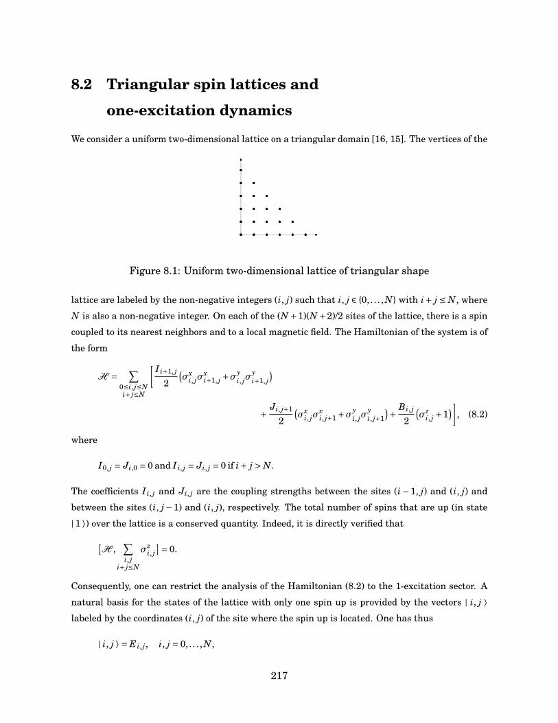
8.2 Triangular spin lattices and
one-excitation dynamics
We consider a uniform two-dimensional lattice on a triangular domain [16, 15]. The vertices of the
Figure 8.1: Uniform two-dimensional lattice of triangular shape
lattice are labeled by the non-negative integers (i, j) such that i, j ∈ 0, . . . , N with i+ j ≤ N, where
N is also a non-negative integer. On each of the (N +1)(N +2)/2 sites of the lattice, there is a spin
coupled to its nearest neighbors and to a local magnetic field. The Hamiltonian of the system is of
the form
H = ∑0≤i, j≤Ni+ j≤N
[ I i+1, j
2(σx
i, jσxi+1, j +σy
i, jσyi+1, j
)
+ Ji, j+1
2(σx
i, jσxi, j+1 +σy
i, jσyi, j+1
)+ Bi, j
2(σz
i, j +1)]
, (8.2)
where
I0, j = Ji,0 = 0 and I i, j = Ji, j = 0 if i+ j > N.
The coefficients I i, j and Ji, j are the coupling strengths between the sites (i−1, j) and (i, j) and
between the sites (i, j−1) and (i, j), respectively. The total number of spins that are up (in state
| 1 ⟩) over the lattice is a conserved quantity. Indeed, it is directly verified that
[H ,
∑i, j
i+ j≤N
σzi, j
]= 0.
Consequently, one can restrict the analysis of the Hamiltonian (8.2) to the 1-excitation sector. A
natural basis for the states of the lattice with only one spin up is provided by the vectors | i, j ⟩labeled by the coordinates (i, j) of the site where the spin up is located. One has thus
| i, j ⟩ = E i, j, i, j = 0, . . . , N,
217
where E i, j is the (N +1)× (N +1) matrix that has a 1 in the (i, j) entry and zeros everywhere else.
The 1-excitation eigenstates of H are denoted by | xs,t ⟩ and are defined by
H | xs,t ⟩ = xs,t| xs,t ⟩, (8.3)
where xs,t is the energy eigenvalue. The expansion of the states | xs,t ⟩ in the | i, j ⟩ basis is written
as
| xs,t ⟩ =∑
0≤i, j≤Ni+ j≤N
Mi, j(s, t)| i, j ⟩.
Since both bases | xs,t ⟩ and | i, j ⟩ are orthonormal, the transition matrix Mi, j(s, t) is unitary. The
energy eigenvalue equation (8.3) imposes that the expansion coefficients Mi, j(s, t) satisfy the 5-
term recurrence relation
xs,tMi, j(s, t)= I i+1, jMi+1, j(s, t)+ Ji, j+1Mi, j+1(s, t)
+Bi, jMi, j(s, t)+ I i, jMi−1, j(s, t)+ Ji, jMi, j−1(s, t). (8.4)
In the following, we shall identity systems specified by the coupling strengths I i, j, Ji, j, and Bi, j
for which the spectrum xs,t and coefficients Mi, j(s, t) can be exactly determined.
8.3 Representations of O(3) on oscillator states and or-
thogonal polynomials
Consider the eigenstates
| n1,n2,n3 ⟩ =| n1 ⟩⊗| n2 ⟩⊗| n3 ⟩, n1,n2,n3 = 0,1, . . . ,
of the three-dimensional isotropic oscillator Hamiltonian
Hosc = a†1a1 +a†
2a2 +a†3a3,
with Hosc| n1,n2,n3 ⟩ = N| n1,n2,n3 ⟩ where the eigenvalue is N = n1 +n2 +n3. Recall that
ai| ni ⟩ =pni| ni ⟩, a†
i | ni ⟩ =√
ni +1| ni +1 ⟩.
Consider R ∈O(3), a rotation matrix. Define U(R) the unitary representation of O(3) by
U(R)aiU†(R)=3∑
k=1Rkiak,
U(R)a†iU
†(R)=3∑
k=1Rkia
†k.
(8.5)
218
It is directly seen from the above that U(RS) = U(R)U(S) for R and S in O(3), as should be for
a representation. Furthermore, one has U(R)U†(R) =U†(R)U(R) = 1. The oscillator Hamiltonian
Hosc is obviously invariant under rotations, i.e.
U(R)HoscU†(R)= Hosc,
and thus any rotation stabilizes the energy eigenspaces of Hosc. The basis vectors for the eigen-
subspaces of Hosc with a fixed value of the energy N denoted by
| i, j ⟩N =| i, j, N − i− j ⟩,
transform reducibly among themselves under the action of the rotations. Consider the matrix
elements of U(R) in the basis | i, j ⟩N | i, j = 0, . . . , N; i+ j ≤ N. These matrix elements can be cast
in the form
N⟨ s, t |U(R) | i, j ⟩N =Ws,t;N Pi, j(s, t; N), (8.6)
where P0,0(s, t; N) ≡ 1 and Ws,t;N = N⟨ s, t | U(R) | 0,0 ⟩N . When no confusion can arise, we shall
drop the explicit dependence of U(R) on R to ease the notation.
8.3.1 Calculation of Ws,t;N
Let us first calculate the amplitude Ws,t;N . To that end, consider the matrix element
N−1⟨ s, t |Ua1 | 0,0 ⟩N
One has on the one hand
N−1⟨ s, t |Ua1 | 0,0 ⟩N = 0.
On the other hand, one can write
N−1⟨ s, t |Ua1 | 0,0 ⟩N = N−1⟨ s, t |Ua1U†U | 0,0 ⟩N
= R11p
s+1 N⟨ s+1, t |U | 0,0 ⟩N +R21p
t+1 N⟨ s, t+1 |U | 0,0 ⟩N
+R31p
N − s− t N⟨ s, t |U | 0,0 ⟩N .
Combining the two equations above, one obtains
R11p
s+1Ws+1,t;N +R21p
t+1Ws,t+1;N +R31p
N − s− tWs,t;N = 0.
Similarly, using N−1⟨ s, t |U(R)a2 | 0,0 ⟩N = 0, one finds
R12p
s+1Ws+1,t;N +R22p
t+1Ws,t+1;N +R32p
N − s− tWs,t;N = 0.
219
Recalling that∑3
k=1 RksRkt = δst, i.e. that Ws,t;N is “essentially orthogonal” to the 1st and 2nd
column of R, one obtains
Ws,t;N = CRs
13R t23RN−s−t
33ps!t!(N − s− t)!
.
The constant C can be found from the normalization condition
1= N⟨ 0,0 |U†U | 0,0 ⟩N
= ∑s+t≤N
N⟨ 0,0 |U† | s, t ⟩N N⟨ s, t |U | 0,0 ⟩N
= ∑s+t≤N
|Ws,t;N |2,
and the trinomial theorem
(x+ y+ z)N = ∑i+ j≤N
N!i! j!(N − i− j)!
xi y j zN−i− j,
giving C =pN! and thus
Ws,t;N =(
Ns, t
)1/2
Rs13R t
23RN−s−t33 , (8.7)
where(Ns, t
)= N!
s!t!(N − s− t)!.
8.3.2 Raising relations
One can show that the functions Pi, j(s, t; N) appearing in the matrix elements (8.6) are polynomi-
als of the discrete variables s and t. One can write
N⟨ s, t |Ua†1 | i, j ⟩N−1 =
pi+1Ws,t;N Pi+1, j(s; t, N),
and also
N⟨ s, t |Ua†1 | i, j ⟩N−1 = N⟨ s, t |Ua†
1U†U | i, j ⟩N−1 =3∑
`=1R`,1 N⟨ s, t | a†
`U | i, j ⟩N−1.
Using (8.6) and (8.7), the two equations above yield
√N(i+1)Pi+1, j(s, t; N)= R11
R13sPi, j(s−1, t; N −1)
+ R21
R23tPi, j(s, t−1; N −1)+ R31
R33(N − s− t)Pi, j(s, t; N −1).
220
A similar relation is obtained starting instead from the matrix element N⟨ s, t |Ua†2 | i, j ⟩N−1:
√N( j+1) Pi, j+1(s, t; N)= R12
R13sPi, j(s−1, t; N −1)
+ R22
R23tPi, j(s, t−1; N −1)+ R32
R33(N − s− t)Pi, j(s, t; N −1).
The two equations above show that the functions Pi, j(s, t; N) are polynomials of total degree i+ j
in the two variables s, t. Indeed, they allow to construct the Pi, j(s, t; N) step by step from P0,0 = 1
by iterations that only involve multiplications by the variables s and t.
8.3.3 Orthogonality relation
The fact that the polynomials Pi, j(s, t; N) are orthogonal follows from the unitarity of the repre-
sentation U(R) and from the fact that the states | i, j ⟩N are orthonormal. The relation
N⟨ i′, j′ |U†U | i, j ⟩N
= ∑s+t≤N
N⟨ i′, j′ |U† | s, t ⟩N N⟨ s, t |U | i, j ⟩N = δii′δ j j′ ,
translates into
∑0≤s,t≤Ns+t≤N
ωs,t;N Pi, j(s, t; N)Pi′, j′(s, t; N)= δii′δ j j′ .
Thus the Pi, j(s, t; N) are polynomials of two discrete variables that are orthogonal on the finite
grid s+ t ≤ N with respect to the trinomial distribution
ωs,t;N =W2s,t;N =
(Ns, t
)R2s
13R2t23R2(N−s−t)
33 .
They provide a two-variable generalization of the one-variable Krawtchouk polynomials which are
orthogonal with respect to the binomial distribution [14, 11, 10, 9, 4, 12].
8.4 Recurrence relations and exact solutions
of 1-excitation dynamics
We shall now derive the recurrence relations satisfied by the polynomials Pi, j(s, t; N) and compare
them with (8.4). Consider the matrix element N⟨ s, t | a†1a1U | i, j ⟩N . One has
N⟨ s, t | a†1a1U | i, j ⟩N = s N⟨ s, t |U | i, j ⟩N .
221
Using (8.5), one has also
N⟨ s, t | a†1a1U | i, j ⟩N =
3∑m,n=1
R1mR1n N⟨ s, t |Ua†man | i, j ⟩N .
Equating the RHS of the two above equations and using the expression (8.6) for the matrix ele-
ments, one finds
sPi, j(s, t; N)= [R2
11 i+R212 j+R2
13(N − i− j)]Pi, j(s, t; N)
+R11R13
[αi+1, j Pi+1, j(s, t; N)+αi, j Pi−1, j(s, t; N)
]+R12R13
[βi, j+1 Pi, j+1(s, t; N)+βi, jPi, j−1(s, t; N)
](8.8)
+R11R12
[γi, j+1 Pi−1, j+1(s, t; N)+γi+1, j Pi+1, j−1(s, t; N)
],
where
αi, j =√
i(N − i− j+1), βi, j =√
j(N − i− j+1),
γi, j =√
i j.
Proceeding likewise with N⟨ s, t | a†2a2U | i, j ⟩N , one obtains
tPi, j(s, t; N)= [R2
21 i+R222 j+R2
23(N − i− j)]Pi, j(s, t; N)
+R21R23
[αi+1, jPi+1, j(s, t; N)+αi, jPi−1, j(s, t; N)
]+R22R23
[βi, j+1Pi, j+1(s, t; N)+βi, jPi, j−1(s, t; N)
](8.9)
+R21R22
[γi, j+1Pi−1, j+1(s, t; N)+γi+1, jPi+1, j−1(s, t; N)
].
Upon combining the recurrence relations (8.8) and (8.9), one can eliminate the non nearest-
neighbor terms Pi−1, j+1(s, t; N) and Pi+1, j−1(s, t; N) to find
(R21R22s−R11R12t)Pi, j(s, t; N)=[R21R22(R2
11 −R213)−R11R12(R2
21 −R223)] i+ [R21R22(R2
12 −R213)−R11R12(R2
22 −R223)] j
+ [R21R22R213 −R11R12R2
23]NPi, j(s, t; N)
+R21R22R11R13 −R11R12R21R23
×
[αi, jPi−1, j(s, t; N)+αi+1, jPi+1, j(s, t; N)
]+
R21R22R12R13 −R11R12R22R23
[βi, j Pi, j−1(s, t; N)+βi, j+1 Pi, j+1(s, t; N)
].
It is readily noted that the above relation is of the same form as the 5-term recurrence equation
(8.4) that one has to solve to obtain the 1-excitation dynamics of the spin lattices governed by the
222
Hamiltonian (8.2). Take
I i, j = (R21R22R11R13 −R11R12R21R23)αi, j,
Ji, j = (R21R22R12R13 −R11R12R22R23)βi, j,(8.10)
and
Bi, j =[R21R22(R2
11 −R213)−R11R12(R2
21 −R223)]i
+ [R21R22(R212 −R2
13)−R11R12(R222 −R2
23)] j+ [R21R22R213 −R11R12R2
23]N. (8.11)
Our polynomial analysis shows that the spectrum of the Hamiltonian (8.2) with couplings (8.10),
(8.11) is given by
xs,t = R21R22s−R11R12t, s, t ∈ 0, . . . , N,
with s+ t ≤ Nand that the unitary expansion coefficients are
Mi, j(s, t)= N⟨ s, t |U(R) | i, j ⟩N =Ws,t;N Pi, j(s, t; N).
The rotation matrix elements Ri j are parameters. If one takes for instance
R =
12 −
p2
4 −12 −
p2
412
−12 −
p2
412 −
p2
412
12
12
p2
2
, (8.12)
one has in particular
R21R22 = R11R12 =−18
, R13 = R23 = 12
,
and
xs,t = 18
(t− s), I i, j =− 116
√i(N − i− j+1),
Bi, j = −1
8p
2( j− i), Ji, j = 1
16
√j(N − i− j+1).
Note that the rotation R specified by (8.12) is improper since detR =−1.
8.5 State transfer
Knowing the 1-excitation dynamics for the particular class of spin lattices, one can determine the
transition amplitudes. Let f(i, j),(k,`)(T) denote the transition amplitude for the excitation at site
223

(i, j) to be found at the site (k,`) after some time T. One can write
f(i, j),(k,`)(T)= ⟨ i, j | e−iTH | k,` ⟩= ∑
s+t≤N⟨ i, j | e−iTH | xs,t ⟩⟨ xs,t | k,` ⟩
= ∑s+t≤N
Mi, j(s, t) Mk,`(s, t) e−iTxs,t
= ∑s+t≤N
N⟨ s, t |U(R) | i, j ⟩N N⟨ s, t |U(R) | k,` ⟩N e−iTxs,t ,
with xs,t = R21R22s−R11R12t. Typically one wishes to transfer state from a given site taken to
be (0,0). Using the expression (8.7) for Ws,t;N , the transition amplitude from the site (0,0) to an
arbitrary site (i, j) is seen to be of the form
f(0,0),(i, j) = RN33
∑s+t≤N
√√√√(Ns, t
)(R13z1
R33
)s (R23z2
R33
)t
N⟨ s, t |U(R) | i, j ⟩N
where we have taken
z1 = e−iR21R22T , z2 = eiR11R12T . (8.13)
Introduce another variable u such that s+ t+u = N as well as an auxiliary variable z3. Let
α1 = R13z1, α2 = R23z2, α3 = R33z3.
and define
G i, j;N (α1,α2,α3)= ∑s,t,u
s+t+u=N
√N!
s!t!u!⟨ s, t,u |U(R) | i, j,k ⟩αs
1αt2α
u3 , (8.14)
with i+ j+ k = N. It is seen that G i, j;N (α1,α2,α3) is a generating function for N⟨ s, t |U(R) | i, j ⟩N
and that
f(0,0),(i, j) =G i, j;N (R13z1,R23z2,R33) z3 = 1. (8.15)
The generating function G i, j;N (α1,α2,α3) is readily computed in the representation framework.
Using (8.14), one writes
G i, j;N (α1,α2,α3)=p
N!∑
s+t+u=N⟨ 0,0,0 | (α1a1)s
s!(α2a2)t
t!(α3a3)u
u!U | i, j,k ⟩
=p
N! ⟨ 0,0,0 |UU†e(α1a1+α2a2+α3a3)U | i, j,k ⟩,
since U keeps N fixed and since the states are orthonormal. Because U | 0,0,0 ⟩ =| 0,0,0 ⟩ and
U†e∑`α`a`U = e
∑`α`Ua`U† = e
∑pβpap
224
with βp =∑`R`pα`, one can write
G i, j;N (α1,α2,α3)=p
N!⟨ 0,0,0 | eβ1a1+β2a2+β3a3 | i, j,k ⟩
=p
N!∑
`,m,n
β`1βm2 β
n3p
`!m!n!⟨ `,m,n | i, j,k ⟩,
which gives
G i, j;N (α1,α2,α3)=(
Ni, j
)1/2
βi1β
j2β
N−i− j3 ,
since i+ j+k = N. Consequently, we have
G i, j;N (α1,α2,α3)=√√√√(
Ni, j
)(R11α1 +R21α2 +R31α3)i
× (R12α1 +R22α2 +R32α3) j(R13α1 +R23α2 +R33α3)N−i− j.
In view of (8.15), we have obtained the following formula for the transition amplitude
f(0,0),(i, j)(T)=√√√√(
Ni, j
)(R11R13z1 +R21R23z2 +R31R33)i
× (R12R13z1 +R22R23z2 +R32R33) j(R213z1 +R2
23z2 +R233)N−i− j,
with z1 and z2 given by (8.13). Let R21R22 = R11R12 and take T = πR11R12
so that z1 = z2 =−1. We
have
f(0,0),(i, j)
(π
R11R12
)=
√√√√(Ni, j
)(−R11R13 −R21R23 +R31R33)i
× (−R12R13 −R22R23 +R32R33) j(−R213 −R2
23 +R233)N−i− j.
If one adds to R21R22 = R11R12 the condition R33 = p2/2, this implies that f(0,0),(i, j)
(π
R11R12
)= 0
unless i+ j = N since (−R213 −R2
23 +R233) = 0. These conditions were met by the rotation matrix
considered in (8.12). With these conditions, the amplitude reads
f(0,0),(i, j)
(π
R11R12
)=
√√√√(Ni, j
)(p
2R31)i(p
2R32) jδi+ j,N ,
and the output excitation distributes binomially on the site of the boundary hypotenuse. Hence
for the values of the parameters such that R21R22 = R11R12 and R33 =p2/2, the Hamiltonian H
with non-homogeneous couplings (8.10) and (8.11) will dynamically evolve the state | 0,0 ⟩ in timeπ
R11R12to any one of the states | i, N − i ⟩ with probability 1. As a consequence∣∣∣ f(0,0),(i, j)
(π
R11R12
)∣∣∣2 = 0, when i+ j < N,
which is akin to perfect transfer. It can be shown that the bivariate Krawtchouk polynomials are
symmetric for these values of the parameters [16].
225
8.6 Conclusion
We have shown that the solutions of the 1-excitation dynamics for a particular class of spin net-
works with inhomogeneous couplings is tied to multivariate orthogonal polynomials and we have
provided an illustration of the theory of multivariate Krawtchouk polynomials based on the rep-
resentations of O(n) on oscillator states. For more details on the connection between orthogonal
polynomials and perfect state transfer, the reader may wish to consult [19, 16, 17]. For a detailed
account of the relation between multivariate orthogonal polynomials and Lie group representa-
tions, the reader is referred to [7, 8, 6, 5].
References
[1] C. Albanese, M. Christandl, N. Datta, and A. Ekert. Mirror Inversion of Quantum States in
Linear Registers. Phys. Rev. Lett., 93:230502, 2004.
[2] S. Bose. Quantum communication through spin chain dynamics: an introductory overview.
Contemp. Phys., 48:13–30, 2007.
[3] R. Chakrabarti and J. Van der Jeugt. Quantum communication through a spin chain with
interaction determined by a Jacobi matrix. J. Phys. A: Math. Theor., 438:085302, 2010.
[4] P. Diaconis and R. C. Griffiths. An introduction to multivariate Krawtchouk polynomials and
their applications. J. Stat. Plann. Inf., 2014.
[5] V. X. Genest, H. Miki, L. Vinet, and A. Zhedanov. The multivariate Charlier polynomials as
matrix elements of the Euclidean group representation on oscillator states. J. Phys. A: Math.
Theor., 47:215204, 2014.
[6] V. X. Genest, H. Miki, L. Vinet, and A. Zhedanov. The multivariate Meixner polynomials as
matrix elements of SO(d,1) representations on oscillator states. J. Phys. A: Math. Theor.,
47:045207, 2014.
[7] V. X. Genest, L. Vinet, and A. Zhedanov. The multivariate Krawtchouk polynomials as matrix
elements of the rotation group representations on oscillator states. J. Phys. A: Math. Theor.,
46:505203, 2013.
[8] V. X. Genest, L. Vinet, and A. Zhedanov. Interbasis expansions for the isotropic 3D harmonic
oscillator and bivariate Krawtchouk polynomials. J. Phys. A: Math. Theor., 47:025202, 2014.
226
[9] R. C. Griffiths. Orthogonal Polynomials on the Multinomial Distribution. Aus. J. Stat., 13:27–
35, 1971.
[10] A. Grünbaum. The Rahman Polynomials Are Bispectral. SIGMA, 302:65–75, 2007.
[11] A. Grünbaum and M. Rahman. A System of Multivariable Krawtchouk polynomials and a
Probabilistic Application. SIGMA, 7:119–135, 2011.
[12] P. Iliev and P. Terwilliger. The Rahman polynomials and the Lie algebra sl3(C). Trans. Amer.
Math. Soc., 364:4225–4238, 2012.
[13] A. Kay. Perfect, efficient, state transfer and its application as a constructive tool. Int. J. Qtm.
Inf., 8:641–676, 2010.
[14] R. Koekoek, P.A. Lesky, and R.F. Swarttouw. Hypergeometric orthogonal polynomials and
their q-analogues. Springer, 1st edition, 2010.
[15] H. Miki, S. Post, L. Vinet, and A. Zhedanov. A superintegrable finite oscillator in two dimen-
sions with SU(2) symmetry. J. Phys. A: Math. Theor., 46:125207, 2012.
[16] H. Miki, S. Tsujimoto, L. Vinet, and A. Zhedanov. Quantum-state transfer in a two-
dimensional regular spin lattice of triangular shape. Phys. Rev. A, 85:062306, 2012.
[17] S. Post. Quantum perfect state transfer in a 2D lattice. Acta Appl. Math., 2014.
[18] L. Vinet and A. Zhedanov. Almost perfect state transfer in quantum spin chains. Phys. Rev.
A, 86:052319, 2012.
[19] L. Vinet and A. Zhedanov. How to construct spin chains with perfect state transfer. Phys.
Rev. A, 85:012323, 2012.
227

228
Chapitre 9
A superintegrable discrete oscillatorand two-variable Meixnerpolynomials
J. Gaboriaud, V. X. Genest, J. Lemieux et L. Vinet (2015). A superintegrable discrete oscillator
and two-variable Meixner polynomials. Soumis au Journal of Physics A: Mathematical and Theo-
retical.
Abstract. A superintegrable, discrete model of the quantum isotropic oscillator in two-dimensions
is introduced. The system is defined on the regular, infinite-dimensional N×N lattice. It is gov-
erned by a Hamiltonian expressed as a seven-point difference operator involving three parame-
ters. The exact solutions of the model are given in terms of the two-variable Meixner polynomials
orthogonal with respect to the negative trinomial distribution. The constants of motion of the
system are constructed using the raising and lowering operators for these polynomials. They are
shown to generate an su(2) invariance algebra. The two-variable Meixner polynomials are seen to
support irreducible representations of this algebra. In the continuum limit, where the lattice con-
stant tends to zero, the standard isotropic quantum oscillator in two dimensions is recovered. The
limit process from the two-variable Meixner polynomials to a product of two Hermite polynomials
is carried out by involving the bivariate Charlier polynomials.
9.1 Introduction
The purpose of this paper is to present a discrete model of the two-dimensional quantum oscillator
that is both superintegrable and exactly solvable. The wavefunctions of this system will be given
229
in terms of the two-variable Meixner polynomials and the constants of motion will be seen to
satisfy the su(2) algebra.
A considerable amount of literature can be found on superintegrable systems and there is a
sustained interest in enlarging the documented set of models with that property. Recall that a
quantum system with d degrees of freedom governed by a Hamiltonian H is said to be super-
integrable if it possesses, including H itself, 2d−1 algebraically independent constants of motion,
that is operators that commute with the Hamiltonian. The quintessential example of a quantum
superintegrable system is the two-dimensional harmonic oscillator, whose constants of motion
generate the su(2) algebra. One of the motivating observations behind the study of superinte-
grable systems is that they are exactly solvable, which makes them prime candidates for modeling
purposes. Also of importance is the fact that these systems form a bedrock for the analysis of sym-
metries, of the associated algebraic structures and their representations, and of special functions.
The majority of quantum superintegrable models cataloged so far comprises continuous systems,
but there has also been some progress in the study of discrete systems [18, 19]; for a review on
superintegrable systems (mostly continuous ones) and their applications, see [20].
In the past years, several discrete models of the one-dimensional quantum oscillator, either
finite or infinite, were introduced [2, 5, 14, 15]. The most studied system, originally proposed
in [6] as a model of multimodal waveguides with a finite number of sensor points, has su(2) as
its dynamical algebra. In this model, the Hamiltonian, the position and momentum operators
are expressed in terms of su(2) generators, the eigenstates of the system are the basis vectors
of unitary irreducible representations of su(2) and the wavefunctions are expressed in terms of
the one-variable Krawtchouk polynomials. As a result, the Hamiltonian has a finite number of
eigenvalues and the spectra of the position and momentum operators are both discrete and finite.
Germane to the present paper is also the discrete oscillator model based on the univariate Meixner
polynomials and related to the su(1,1) algebra considered in [2]. See also [16], where instead the
Meixner-Pollaczek polynomials are involved.
The Krawtchouk one-dimensional finite/discrete oscillator has been exploited to construct fi-
nite/discrete systems in two dimensions. Two approaches have been used. The first approach
consist in taking the direct product of two one-dimensional su(2) systems to obtain a system de-
fined on a square grid with su(2)⊕su(2) as its dynamical algebra [3]. In the second approach [4],
the isomorphism so(4) ∼= su(2)⊕su(2) is exploited to obtain a description of the finite oscillator on
the square grid in terms of discrete radial and angular coordinates. In the continuum limit, both
of these models tend to the standard two-dimensional oscillator. However, they do not exhibit the
su(2) invariance, or symmetry algebra, of the standard two-dimensional oscillator.
Recently another discrete and finite model of the two-dimensional oscillator was proposed [19].
This model is defined on a triangular lattice of a given size and, like the standard oscillator in two
230
dimensions, it is superintegrable and has su(2) for symmetry algebra. The wavefunctions of the
model, which support irreducible representations of su(2) at fixed energy, are given in terms of
the two-variable Krawtchouk polynomials introduced by Griffiths [10]. These polynomials of two
discrete variables are orthogonal with respect to the trinomial distribution. As required, this
model tends to the standard two-dimensional oscillator in the continuum limit.
Shortly after [19] appeared, it was recognized that the d-variable Krawtchouk polynomials of
Griffiths arise as matrix elements of the unitary representations of the rotation group SO(d+1) on
oscillator states [9]. This interpretation has provided a cogent framework for the characterization
of these orthogonal functions and has led to a number of new identities. The group theoretical in-
terpretation was also extended to two other families of discrete multivariate polynomials: the mul-
tivariate Meixner and Charlier polynomials, orthogonal with respect to the negative multinomial
and multivariate Poisson distributions, respectively. The multi-variable Meixner polynomials, also
introduced by Griffiths [11], were shown to arise as matrix elements of unitary representations of
the pseudo-rotation group SO(d,1) on oscillator states [8]. As for the multivariate Charlier poly-
nomials, they were first introduced as matrix elements of unitary representations of the Euclidean
group on oscillator states [7]. Let us note that these family of multivariate polynomials also arise
in probability theory in connection with the so-called Lancaster distributions [12].
In this paper, we present a new discrete oscillator model in two-dimensions based on the two-
variable Meixner polynomials. The model is defined on the regular infinite-dimensional N×Nlattice. It is governed by a Hamiltonian involving three independent parameters expressed as a
7-point difference operator. This operator is obtained by combining the two independent difference
equations satisfied by the bivariate Meixner polynomials. By construction, the wavefunctions of
the model are given in terms of these two-variable polynomials. The energies of the system are
given by the non-negative integers N = 0,1,2, . . . and exhibit a (N +1)-fold degeneracy. Using the
raising and lowering relations for the two-variable Meixner polynomials, the constants of motion
of the system are constructed and are shown to close onto the su(2) commutation relations. In
the continuum limit, in which the lattice parameter tends to zero, the model contracts to the
standard quantum harmonic oscillator, as required for a discrete oscillator model. The contraction
process is illustrated at the wavefunction level using the two-variable Charlier polynomials in an
intermediary step. The continuum limit is also displayed at the level of operators.
Here is the outline of the paper. In Section two, the essential properties of the two-variable
Meixner polynomials are reviewed. In Section three, the Hamiltonian of the model is defined, the
constants of motion are constructed, and the wavefunctions are illustrated. In Section four, the
continuum limit of the model and wavefunctions is examined. We conclude with an outlook.
231
9.2 The two-variable Meixner polynomials
We now review the properties of the two-variable Meixner polynomials using the formalism and
notation developed in [8]. Let β> 0 be a positive real number and let Λ ∈O(2,1) be a 3×3 pseudo-
rotation matrix. This implies that Λ satisfies
Λ>ηΛ= η,
where η = diag(1,1,−1) and where Λ> denotes the transposed matrix. In general, Λ can be
parametrized by three real numbers akin to the Euler angles. The two-variable Meixner poly-
nomials, denoted by M(β)n1,n2(x1, x2), are defined by the generating function(
1+ Λ11
Λ13z1 + Λ12
Λ13z2
)x1(1+ Λ21
Λ23z1 + Λ22
Λ23z2
)x2(1+ Λ31
Λ33z1 + Λ32
Λ33z2
)−x1−x2−β
=∞∑
n1=0
∞∑n2=0
√(β)n1+n2
n1!n2!M(β)
n1,n2(x1, x2) zn11 zn2
2 , (9.1)
where the Λi j are the entries of the parameter matrix Λ and where (β)n stands for the Pochham-
mer symbol defined as
(β)n =
1 n = 0∏n−1k=0(β+k) n = 1,2,3, . . .
It can be seen from (9.1) that M(β)n1,n2(x1, x2) are polynomials of total degree n1+n2 in the variables
x1 and x2. The functions M(β)n1,n2(x1, x2) satisfy the orthogonality relation
∞∑x1=0
∞∑x2=0
ω(x1, x2) M(β)n1,n2(x1, x2) M(β)
n′1,n′
2(x1, x2)= δn1,n′
1δn2,n′
2, (9.2)
where ω(x1, x2) is the negative trinomial distribution
ω(x1, x2)= (β)x1+x2
x1! x2!(1− c1 − c2)β cx1
1 cx22 , (9.3)
and where the parameters c1, c2 are given by
c1 =(Λ13
Λ33
)2, c2 =
(Λ23
Λ33
)2.
The polynomials M(β)n1,n2(x1, x2) have an explicit expression in terms of Aomoto–Gelfand hypergeo-
metric series [13]. This expression reads
M(β)n1,n2(x1, x2)= (−1)n1+n2
√(β)n1+n2
n1!n2!
(Λ31
Λ33
)n1(Λ32
Λ33
)n2
× ∑µ,ν,ρ,σ>0
(−n1)µ+ν(−n2)ρ+σ(−x1)µ+ρ(−x2)ν+σµ!ν!ρ!σ! (β)µ+ν+ρ+σ
(1−u11)µ(1−u21)ν(1−u12)ρ(1−u22)σ, (9.4)
232
where the parameters ui j are given by
u11 = Λ11Λ33
Λ13Λ31, u12 = Λ12Λ33
Λ13Λ32, u21 = Λ21Λ33
Λ23Λ31, u22 = Λ22Λ33
Λ23Λ32.
Let T±xi
f (xi) = f (xi ±1) for i = 1,2 be the discrete shift operators in the variables x1 and x2.
Introduce the two intertwining operators A(i)+ defined as
A(i)+ = Λ1i
Λ13x1T−
x1+ Λ2i
Λ23x2T−
x2− Λ3i
Λ33(x1 + x2 +β) I, i = 1,2, (9.5)
where I stands for the identity operator. On the bivariate polynomials M(β)n1,n2(x1, x2), these opera-
tors have the actions
A(1)+ M(β+1)
n1,n2 (x1, x2)=√β (n1 +1) M(β)
n1+1,n2(x1, x2),
A(2)+ M(β+1)
n1,n2 (x1, x2)=√β (n2 +1) M(β)
n1,n2+1(x1, x2).(9.6)
Introduce also the two intertwining operators A(i)− defined in the following way:
A(i)− =Λ1iΛ13 T+
x1+Λ2iΛ23 T+
x2− (Λ1iΛ13 +Λ2iΛ23) I, i = 1,2. (9.7)
These operators act as follows on the bivariate Meixner polynomials
A(1)− M(β)
n1,n2(x1, x2)=√
n1
βM(β+1)
n1−1,n2(x1, x2),
A(2)− M(β)
n1,n2(x1, x2)=√
n2
βM(β+1)
n1,n2−1(x1, x2).
(9.8)
The intertwining operators (9.5) and (9.7) can be combined to produce the two commuting dif-
ference operators Y1 and Y2 that are diagonalized by the bivariate Meixner polynomials. These
operators are defined as
Yi = A(i)+ A(i)
− , i = 1,2. (9.9)
Explicitly, one finds
Yi =(Λ1iΛ2iΛ23
Λ13
)x1T−
x1T+
x2+
(Λ1iΛ2iΛ13
Λ23
)x2T+
x1T−
x2−
(Λ1iΛ3iΛ33
Λ13
)x1T−
x1
−(Λ2iΛ3iΛ33
Λ23
)x2T−
x2−
(Λ1iΛ3iΛ13
Λ33
)(x1 + x2 +β)T+
x1
−(Λ2iΛ3iΛ23
Λ33
)(x1 + x2 +β)T+
x2+ [Λ2
1i x1 +Λ22i x2 +Λ2
3i (x1 + x2 +β)]I. (9.10)
The eigenvalue equations read
Y1 M(β)n1,n2(x1, x2)= n1 M(β)
n1,n2(x1, x2), Y2 M(β)n1,n2(x1, x2)= n2 M(β)
n1,n2(x1, x2), (9.11)
where n1, n2 are non-negative integers. Let us note that the operators Y1 and Y2 fully characterize
the polynomials M(β)n1,n2(x1, x2).
233
9.3 A discrete and superintegrable Hamiltonian
We now consider the Hamiltonian obtained by taking the sum of the operators Y1 and Y2 involved
in the eigenvalue equations (9.11). We hence define
H =Y1 +Y2. (9.12)
In principle the Hamiltonian (9.12) involves four independent parameters including β, as any
matrix Λ ∈ O(2,1) depends on three independent parameters. However, it turns out that H es-
sentially depends only on three parameters, including β. This can be seen explicitly as follows.
Consider the following parametrization of Λ in terms of the “Euler angles” ψ, ξ and φ:
Λ(ψ,ξ,φ)=
coshξ 0 sinhξ
0 1 0
sinhξ 0 coshξ
1 0 0
0 coshψ sinhψ
0 sinhψ cosψ
cosφ sinφ 0
−sinφ cosφ 0
0 0 1
. (9.13)
Upon using the expressions (9.10), it is seen that in the parametrization (9.13) the Hamiltonian
(9.12) has the expression
H (ψ,ξ,φ)= sinh2ψ x1T−x1
T+x2+cosh2ψsinh2 ξ x2T+
x1T−
x2
−cosh2ψsinh2 ξ (x1 + x2 +β)T+x1−sinh2ψ (x1 + x2 +β)T+
x2
−cosh2 ξcosh2ψ[x1T−
x1+ x2T−
x2
]+[cosh2ξcosh2ψ x1
+ (cosh2ψ+sinh2 ξ+ cosh2 ξsinh2ψ) x2 +β (sinh2 ξ+ cosh2 ξsinh2ψ)]I,
hence the parameter φ does not explicitly appear in H . The fact that the Hamiltonian (9.12) can
be presented in terms three independent parameters is a manifestation of its superintegrability.
Let JX , JY and JZ be the operators defined as follows.
JX = 12
(A(1)+ A(2)
− + A(2)+ A(1)
−),
JY = 12i
(A(1)+ A(2)
− − A(2)+ A(1)
−),
JZ = 12
(A(1)+ A(1)
− − A(2)+ A(2)
−).
(9.14)
The operators JX , JY and JZ are constants of motion. Indeed, one can verify by a direct calculation
that these operators commute with the Hamiltonian (9.12)
[H , JX ]= 0, [H , JY ]= 0, [H , JZ]= 0.
The symmetry operators JX , JY and JZ satisfy the defining relations of the su(2) algebra. One
has
[JX , JY ]= iJZ , [JY , JZ]= iJX , [JZ , JX ]= iJY . (9.15)
234
In the realization (9.14), the su(2) Casimir operator is related to the Hamiltonian (9.12) through
J2X + J2
Y + J2Z = 1
2H
(H
2+1
). (9.16)
The realization (9.14) of the su(2) algebra (9.15) and the expression (9.16) of the Casimir opera-
tor in terms of the Hamiltonian is very close to the Schwinger realization of su(2) that one finds
when considering the standard two-dimensional quantum harmonic oscillator. The SU(2) sym-
metry (9.15) of the Hamiltonian (9.12) explains why H depends on three parameters instead of
four: the φ parameter in (9.12) has been “rotated away” from the Hamiltonian by the choice of
parametrization (9.13).
By construction, the eigenfunctions of the Hamiltonian (9.12) are expressed in terms of the
two-variable Meixner polynomials M(β)n1,n2(x1, x2). These eigenfunctions Ψ(β)
N,n(x1, x2) are labeled by
the two non-negative integers N and n and read
Ψ(β)N,n(x1, x2)= M(β)
n,N−n(x1, x2),
where n = 0,1, . . . , N and where N = 0,1,2, . . .. One has
H Ψ(β)N,n(x1, x2)= NΨ
(β)N,n(x1, x2), JZΨ
(β)N,n(x1, x2)= (n−N/2)Ψ(β)
N,n(x1, x2). (9.17)
Hence the eigenvalues of H are the non-negative integers N = 0,1,2, . . . and are (N + 1)-times
degenerate. The states ΨN,n(x1, x2) support (N + 1)-dimensional irreducible representations of
su(2). Upon introducing the generators
J± = JX ± iJY ,
it is seen from (9.6) and (9.8) that these operators have the actions
J+Ψ(β)N,n(x1, x2)=
√(n+1)(N −n)Ψ(β)
N,n+1(x1, x2), (9.18)
J−Ψ(β)N,n(x1, x2)=
√n(N −n+1)Ψ(β)
N,n−1(x1, x2). (9.19)
It thus follows that the two-variable Meixner polynomials M(β)n1,n2(x1, x2) support (K+1)-dimensional
unitary representations of su(2) were K = n1 +n2.
In view of (9.2) wavefunctions ΨN,n(x1, x2) are not normalized on the infinite grid (x1, x2) ∈N×N with respect to the standard uniform measure of quantum mechanics. Properly normalized
wavefunctions Υ(β)N,n(x1, x2) are obtained by taking
Υ(β)N,n(x1, x2)=
√ω(x1, x2) M(β)
n,N−n(x1, x2), (9.20)
where ω(x1, x2) is given by (9.3). One then has the orthogonality and completeness relations [8]∞∑
x1=0
∞∑x2=0
Υ(β)N,n(x1, x2)Υ(β)
N ′,n′(x1, x2)= δnn′δNN ′ ,
∞∑N=0
N∑n=0
Υ(β)N,n(x1, x2)Υ(β)
N,n(x′1, x′2)= δx1,x′1δx2,x′2 .
235
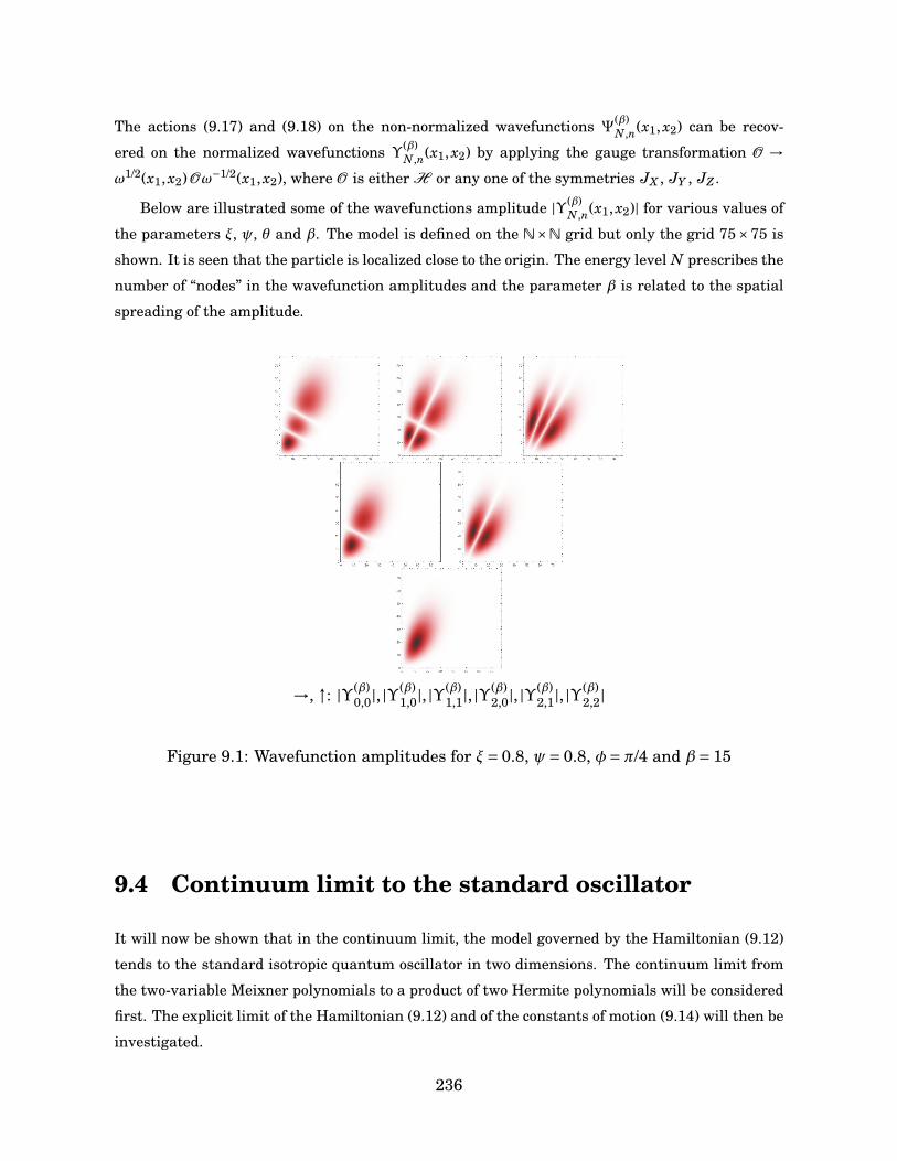
The actions (9.17) and (9.18) on the non-normalized wavefunctions Ψ(β)N,n(x1, x2) can be recov-
ered on the normalized wavefunctions Υ(β)N,n(x1, x2) by applying the gauge transformation O →
ω1/2(x1, x2) Oω−1/2(x1, x2), where O is either H or any one of the symmetries JX , JY , JZ .
Below are illustrated some of the wavefunctions amplitude |Υ(β)N,n(x1, x2)| for various values of
the parameters ξ, ψ, θ and β. The model is defined on the N×N grid but only the grid 75×75 is
shown. It is seen that the particle is localized close to the origin. The energy level N prescribes the
number of “nodes” in the wavefunction amplitudes and the parameter β is related to the spatial
spreading of the amplitude.
→, ↑: |Υ(β)0,0|, |Υ
(β)1,0|, |Υ
(β)1,1|, |Υ
(β)2,0|, |Υ
(β)2,1|, |Υ
(β)2,2|
Figure 9.1: Wavefunction amplitudes for ξ= 0.8, ψ= 0.8, φ=π/4 and β= 15
9.4 Continuum limit to the standard oscillator
It will now be shown that in the continuum limit, the model governed by the Hamiltonian (9.12)
tends to the standard isotropic quantum oscillator in two dimensions. The continuum limit from
the two-variable Meixner polynomials to a product of two Hermite polynomials will be considered
first. The explicit limit of the Hamiltonian (9.12) and of the constants of motion (9.14) will then be
investigated.
236
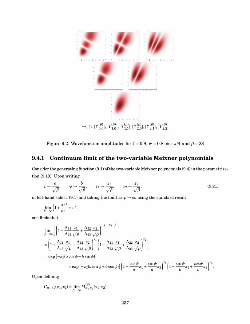
→, ↑: |Υ(β)0,0|, |Υ
(β)1,0|, |Υ
(β)1,1|, |Υ
(β)2,0|, |Υ
(β)2,1|, |Υ
(β)2,2|
Figure 9.2: Wavefunction amplitudes for ξ= 0.8, ψ= 0.8, φ=π/4 and β= 28
9.4.1 Continuum limit of the two-variable Meixner polynomials
Consider the generating function (9.1) of the two-variable Meixner polynomials (9.4) in the parametriza-
tion (9.13). Upon writing
ξ→ a√β
, ψ→ b√β
, z1 → z1√β
, z2 → z2√β
, (9.21)
in left-hand side of (9.1) and taking the limit as β→∞ using the standard result
limk→∞
(1+ x
k
)k = ex,
one finds that
limβ→∞
[(1+ Λ31
Λ33
z1√β+ Λ32
Λ33
z2√β
)−x1−x2−β
×(1+ Λ11
Λ13
z1√β+ Λ12
Λ13
z2√β
)x1(1+ Λ21
Λ23
z1√β+ Λ22
Λ23
z2√β
)x2 ]= exp
[−z1(acosφ−bsinφ)]
×exp[−z2(asinφ+bcosφ)
](1+ cosφ
az1 + sinφ
az2
)x1(1− sinφ
bz1 + cosφ
bz2
)x2
.
Upon defining
Cn1,n2(x1, x2)= limβ→∞
M(β)n1,n2(x1, x2),
237
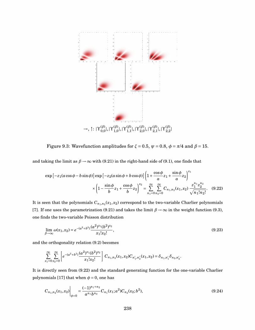
→, ↑: |Υ(β)0,0|, |Υ
(β)1,0|, |Υ
(β)1,1|, |Υ
(β)2,0|, |Υ
(β)2,1|, |Υ
(β)2,2|
Figure 9.3: Wavefunction amplitudes for ξ= 0.5, ψ= 0.8, φ=π/4 and β= 15.
and taking the limit as β→∞ with (9.21) in the right-hand side of (9.1), one finds that
exp[−z1(acosφ−bsinφ)
]exp
[−z2(asinφ+bcosφ)](
1+ cosφa
z1 + sinφa
z2
)x1
×(1− sinφ
bz1 + cosφ
bz2
)x2
=∞∑
n1=0
∞∑n2=0
Cn1,n2(x1, x2)zn1
1 zn22√
n1!n2!. (9.22)
It is seen that the polynomials Cn1,n2(x1, x2) correspond to the two-variable Charlier polynomials
[7]. If one uses the parametrization (9.21) and takes the limit β→∞ in the weight function (9.3),
one finds the two-variable Poisson distribution
limβ→∞
ω(x1, x2)= e−(a2+b2) (a2)x1(b2)x2
x1!x2!, (9.23)
and the orthogonality relation (9.2) becomes
∞∑x1=0
∞∑x2=0
[e−(a2+b2) (a2)x1(b2)x2
x1!x2!
]Cn1,n2(x1, x2)Cn′
1,n′2(x1, x2)= δn1,n′
1δn2,n′
2.
It is directly seen from (9.22) and the standard generating function for the one-variable Charlier
polynomials [17] that when φ= 0, one has
Cn1,n2(x1, x2)∣∣∣∣φ=0
= (−1)n1+n2
an1 bn2Cn1(x1;a2)Cn2(x2;b2), (9.24)
238
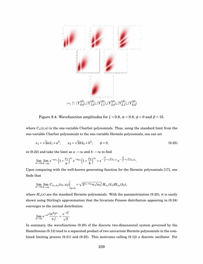
→, ↑: |Υ(β)0,0|, |Υ
(β)1,0|, |Υ
(β)1,1|, |Υ
(β)2,0|, |Υ
(β)2,1|, |Υ
(β)2,2|
Figure 9.4: Wavefunction amplitudes for ξ= 0.8, ψ= 0.8, φ= 0 and β= 15.
where Cn(x;a) is the one-variable Charlier polynomials. Thus, using the standard limit from the
one-variable Charlier polynomials to the one-variable Hermite polynomials, one can set
x1 =p
2ax1 +a2, x2 =p
2bx2 +b2, φ= 0, (9.25)
in (9.22) and take the limit as a →∞ and b →∞ to find
lima→∞ lim
b→∞e−az1
(1+ z1
a
)x1e−bz2
(1+ z2
b
)x2 = e−z212 +p2 x1 z1 e−
z222 +p2 x2 z2 .
Upon comparing with the well-known generating function for the Hermite polynomials [17], one
finds that
lima→∞ lim
b→∞Cn1,n2(x1, x2)
∣∣∣∣φ=0
=√
2n1+n2 n1!n2! Hn1(x1)Hn2(x2),
where Hn(x) are the standard Hermite polynomials. With the parametrization (9.25), it is easily
shown using Stirling’s approximation that the bivariate Poisson distribution appearing in (9.24)
converges to the normal distribution
lima→∞ e−a2 (a2)x1
x1!= e−x2
1
pπ
.
In summary, the wavefunctions (9.20) of the discrete two-dimensional system governed by the
Hamiltonian (9.12) tend to a separated product of two univariate Hermite polynomials in the com-
bined limiting process (9.21) and (9.25). This motivates calling (9.12) a discrete oscillator. For
239
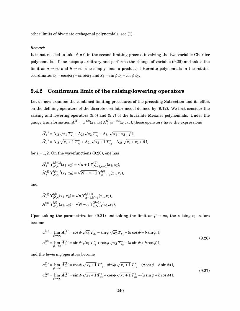
other limits of bivariate orthogonal polynomials, see [1].
Remark
It is not needed to take φ = 0 in the second limiting process involving the two-variable Charlier
polynomials. If one keeps φ arbitrary and performs the change of variable (9.25) and takes the
limit as a → ∞ and b → ∞, one simply finds a product of Hermite polynomials in the rotated
coordinates x1 = cosφ x1 −sinφ x2 and x2 = sinφ x1 −cosφ x2.
9.4.2 Continuum limit of the raising/lowering operators
Let us now examine the combined limiting procedures of the preceding Subsection and its effect
on the defining operators of the discrete oscillator model defined by (9.12). We first consider the
raising and lowering operators (9.5) and (9.7) of the bivariate Meixner polynomials. Under the
gauge transformation A(i)± =ω1/2(x1, x2) A(i)
± ω−1/2(x1, x2), these operators have the expressions
A(i)+ =Λ1i
px1 T−
x1+Λ2i
px2 T−
x2−Λ3i
√x1 + x2 +β I,
A(i)− =Λ1i
√x1 +1 T+
x1+Λ2i
√x2 +1 T+
x2−Λ3i
√x1 + x2 +β I,
for i = 1,2. On the wavefunctions (9.20), one has
A(1)+ Υ
(β+1)N,n (x1, x2)=
pn+1Υ(β)
N+1,n+1(x1, x2),
A(2)+ Υ
(β+1)N,n (x1, x2)=
pN −n+1Υ(β)
N+1,n(x1, x2),
and
A(1)− Υ
(β)N,n(x1, x2)=p
nΥ(β+1)n−1,N−1(x1, x2),
A(2)− Υ
(β)N,n(x1, x2)=
pN −nΥ(β+1)
n,N−1(x1, x2).
Upon taking the parametrization (9.21) and taking the limit as β → ∞, the raising operators
become
a(1)+ = lim
β→∞A(1)+ = cosφ
px1 T−
x1−sinφ
px2 T−
x2− (acosφ−bsinφ) I,
a(2)+ = lim
β→∞A(2)+ = sinφ
px1 T−
x1+cosφ
px2 T−
x2− (asinφ+bcosφ) I,
(9.26)
and the lowering operators become
a(1)− = lim
β→∞A(1)− = cosφ
√x1 +1 T+
x1−sinφ
√x2 +1 T+
x2− (acosφ−bsinφ) I,
a(2)− = lim
β→∞A(1)− = sinφ
√x1 +1 T+
x1+cosφ
√x2 +1 T+
x2− (asinφ+bcosφ) I.
(9.27)
240
A direct calculation shows that these operators satisfy the commutation relations
[a(i)− ,a( j)
+ ]= δi j, [a(i)− ,a( j)
− ]= 0, [a(i)+ ,a( j)
+ ]= 0.
Upon setting x1 =p
2ax1+a2 and x2 =p
2bx2+b2 as in (9.25) and taking the limit as a →∞ and b →∞, it is easily seen that the operators (9.26) and (9.27) become the rotated creation/annihilation
operators
a(1)+ → cosφ a†
1 −sinφ a†2, a(2)
+ → sinφ a†1 +cosφ a†
2,
a(1)− → cosφ a1 −sinφ a2, a(2)
− → sinφ a1 +cosφ a2,
where
ai =xi +∂xip
2, a†
i =xi −∂xip
2,
are the usual creation/annihilation operators. It immediately follows that in the continuum limit
described above in a two-step process, the gauge-transformed Hamiltonian (9.12) and constants
of motion (9.14) obtained through ω(x1, x2)1/2Oω−1/2(x1, x2) tend to the standard two-dimensional
oscillator Hamiltonian and the su(2) generators in the Schwinger realization.
9.5 Conclusion
In this paper, we have introduced and described a discrete model of the oscillator in two-dimensions
based on the bivariate Meixner polynomials. We have shown that this system is superintegrable
and that it has the same symmetry algebra as its continuum limit, the standard isotropic oscilla-
tor in two dimensions. We have established that the two-variable Meixner polynomials form bases
for irreducible representations of su(2). We have detailed the limiting processes by which the two-
variable Meixner polynomials tend to the bivariate Charlier polynomials and by which the latter
tend to a product of standard Hermite polynomials.
In the present paper we have considered for simplicity the two-dimensional case. However,
since the theory of multi-variable Meixner is now well established, it is clear that the model can
be generalized to any dimensions to give a d-dimensional model of the harmonic oscillator with
the same su(d) symmetry as the standard quantum oscillator in d-dimensions. Another possi-
ble generalization would be to consider, instead of (9.12), a discrete anisotropic oscillator with a
Hamiltonian of the form H = Y1 +αY2. It is clear that for rational values of α this model would
still be superintegrable, but would exhibit a higher order symmetry algebra.
241
References
[1] I. Area and E. Godoy. On limit relations between some families of bivariate hypergeometric
orthogonal polynomials. Journal of Physics A: Mathematical and Theoretical, 46(3):035202,
January 2013.
[2] N. Atakishiyev, E. I. Jafarov, S. M. Nagiyev, and K. B. Wolf. Meixner oscillators. Revista
Mexicana de Fisica, 44(33):235–244, June 1998.
[3] N. Atakishiyev, G. Pogosyan, L. E. Vicent, and K. B. Wolf. Finite two-dimensional oscilla-
tor: I. The Cartesian model. Journal of Physics A: Mathematical and General, 34(44):9381,
November 2001.
[4] N. Atakishiyev, G. Pogosyan, L. E. Vicent, and K. B. Wolf. Finite two-dimensional oscillator:
II. The radial model. Journal of Physics A: Mathematical and General, 34(44):9399–9415,
November 2001.
[5] N. Atakishiyev, G. Pogosyan, and K. B. Wolf. Finite models of the oscillator. Physics of
Particles and Nuclei, 36:247–265, 2005.
[6] N. Atakishiyev and K. B. Wolf. Fractional Fourier–Kravchuk transform. Journal of the Opti-
cal Society of America A, 14(7):1467–1477, 1997.
[7] V. X. Genest, H. Miki, L. Vinet, and A. Zhedanov. The multivariate Charlier polynomials
as matrix elements of the Euclidean group representation on oscillator states. Journal of
Physics A: Mathematical and Theoretical, 47(21):215204, May 2014.
[8] V. X. Genest, H. Miki, L. Vinet, and A. Zhedanov. The multivariate Meixner polynomials
as matrix elements of SO(d,1) representations on oscillator states . Journal of Physics A:
Mathematical and Theoretical, 47(4):045207, January 2014.
[9] V. X. Genest, L. Vinet, and A. Zhedanov. The multivariate Krawtchouk polynomials as matrix
elements of the rotation group representations on oscillator states. Journal of Physics A:
Mathematical and Theoretical, 46(50):505203, December 2013.
[10] R. C. Griffiths. Orthogonal Polynomials on the multinomial distribution. Australian Journal
of Statistics, 3(1):27–35, April 1971.
[11] R. C. Griffiths. Orthogonal polynomials on the negative multinomial distribution. Journal of
Multivariate Analysis, 5(2):271–277, June 1975.
242
[12] R. C. Griffiths. Multivariate Poisson–Charlier, Meixner and Hermite–Chebycheff polynomi-
als and Lancaster distributions. ArXiv:1412.3931, 2014.
[13] P. Iliev. Meixner polynomials in several variables satisfying bispectral difference equations.
Advances in Applied Mathematics, 49(1):15–23, July 2012.
[14] E. I. Jafarov and J. Van der Jeugt. Discrete series representations for sl(2|1), Meixner
polynomials and oscillator models. Journal of Physics A: Mathematical and Theoretical,
45(48):485201, December 2012.
[15] E. I. Jafarov, N. I. Stoilova, and J. Van der Jeugt. Finite oscillator models: the Hahn oscillator.
Journal of Physics A: Mathematical and Theoretical, 44(26):265203, July 2011.
[16] A. U. Klimyk. The su(1,1)-models of quantum oscillator. Ukrainian Journal of Physics,
51(10):1019–1027, 2006.
[17] R. Koekoek, P. A. Lesky, and R. F. Swarttouw. Hypergeometric orthogonal polynomials and
their q-analogues. Springer, 2010.
[18] D. Levi, P. Tempesta, and P. Winternitz. Umbral calculus, difference equations and the dis-
crete Schrödinger equation. Journal of Mathematical Physics, 45(11):4077, November 2004.
[19] H. Miki, S. Post, L. Vinet, and A. Zhedanov. A superintegrable finite oscillator in two
dimensions with SU(2) symmetry. Journal of Physics A: Mathematical and Theoretical,
46(12):125207, March 2013.
[20] W. Miller, S. Post, and P. Winternitz. Classical and quantum superintegrability with applica-
tions. Journal of Physics A: Mathematical and Theoretical, 46(42):423001, October 2013.
243

244
Partie II
Systèmes superintégrables avecréflexions
245

Introduction
Un système quantique possédant d degrés de liberté décrit par un hamiltonien H est dit maxi-
malement superintégrable s’il admet 2d−1 opérateurs de symétrie algébriquement indépendants
qui satisfont aux conditions
[Si,H]= 0, i = 1,2, . . . ,2d−1,
où l’un des opérateurs de symétrie est l’hamiltonien lui-même [55]. Pour un système quantique
superintégrable gouverné par un hamiltonien de la forme
H =∆+V ,
où ∆ est l’opérateur de Laplace–Beltrami
∆= 1pg
∑i j∂xi (
pg gi j)∂x j ,
et où gi j est la métrique et V est le potentiel, les symétries seront exprimées en termes d’opérateurs
différentiels. On dira que le système est superintégrable de degré ` si ` est le degré maximal des
opérateurs de symétrie, excluant cette fois l’hamiltonien. Pour un système maximalement super-
intégrable, il est impossible que tous les opérateurs de symétrie soient en involution les uns avec
les autres; ces derniers engendrent donc une algèbre d’invariance non abélienne.
Les systèmes superintégrables sont d’une grande importance, notamment parce qu’ils peuvent
être résolus de manière exacte à la fois analytiquement et algébriquement. Un des exemples
classiques de système maximalement superintégrable (`= 1) est celui de l’oscillateur harmonique
en deux dimensions, dont les constantes du mouvement peuvent être obtenues par la construction
de Schwinger et engendrent l’algèbre su(2) [56].
Lorsque `= 1, les symétries sont de nature géométrique et engendrent une algèbre de Lie. Les
systèmes de ce type sont très bien connus. Lorsque `= 2, l’algèbre d’invariance est généralement
quadratique. En deux dimensions, tous les systèmes superintégrables de ce type ont été identifiés
[57]. Le plus général d’entre eux est connu sous le nom de système générique sur la 2-sphère: tous
les systèmes superintégrables de second ordre en deux dimensions peuvent être obtenus à partir
247
de ce système [58]. On soupçonne également que le système générique sur la 3-sphère joue le
même rôle en trois dimensions.
Dans cette partie de la thèse, on étudie des systèmes superintégrables en deux et trois dimen-
sions qui font intervenir des opérateurs de Dunkl, qui contiennent des réflexions. On utilise les
opérateurs de Dunkl de rang 1. Ces opérateurs dépendent d’un paramètre réel µ≥ 0 et sont définis
par [59]
D i = ∂xi +µi
xi(1−Ri),
où Ri est l’opérateur de réflexion Ri f (xi) = f (−xi). Il est clair que les opérateurs D i sont une
généralisation à un paramètre de la dérivée partielle usuelle, que l’on retrouve lorsque µi = 0.
Dans cette partie de la thèse, on considère les systèmes suivants.
• L’oscillateur de Dunkl dans le plan
H =−12
[D2
1 +D22
]+ 1
2(x2
1 + x22).
• L’oscillateur singulier de Dunkl dans le plan
H =−12
[D2
1 +D22
]+ 1
2(x2
1 + x22)+ (α1 +β1R1)
2x21
+ (α2 +β2R2)2x2
2.
• L’oscillateur de Dunkl en trois dimensions
H =−12
[D2
1 +D22 +D2
3
]+ 1
2(x2
1 + x22 + x2
3).
• Le système générique sur la 2-sphère avec réflexions
H = J21 + J2
2 + J23 + µ1
x21
(µ1 −R1)+ µ2
x22
(µ2 −R2)+ µ3
x23
(µ3 −R3),
où J1, J2 et J3 sont les opérateurs de moment angulaire
J1 = 1i(x2∂x3 − x3∂x2), J2 = 1
i(x3∂x1 − x1∂x3), J3 = 1
i(x1∂x2 − x2∂x1).
On montre que tous ces systèmes sont superintégrables et exactement résolubles, malgré la présence
des opérateurs de réflexion. On obtient dans chaque cas leurs symétries, les algèbres d’invariance
qu’elles engendrent et leurs représentations. On illustre aussi en quoi ces modèles sont une vitrine
pour les polynômes du tableau de Bannai–Ito.
248
Chapitre 10
The Dunkl oscillator in the plane I :superintegrability, separatedwavefunctions and overlapcoefficients
V. X. Genest, M. E. H. Ismail, Luc Vinet et A. Zhedanov (2013). The Dunkl oscillator in the plane
I : superintegrability, separated wavefunctions and overlap coefficients. Journal of Physics A:
Mathematical and Theoretical 46 145201
Abstract. The isotropic Dunkl oscillator model in the plane is investigated. The model is defined
by a Hamiltonian constructed from the combination of two independent parabosonic oscillators.
The system is superintegrable and its symmetry generators are obtained by the Schwinger con-
struction using parabosonic creation/annihilation operators. The algebra generated by the con-
stants of motion, which we term the Schwinger-Dunkl algebra, is an extension of the Lie algebra
u(2) with involutions. The system admits separation of variables in both Cartesian and polar coor-
dinates. The separated wavefunctions are respectively expressed in terms of generalized Hermite
polynomials and products of Jacobi and Laguerre polynomials. Moreover, the so-called Jacobi-
Dunkl polynomials appear as eigenfunctions of the symmetry operator responsible for the separa-
tion of variables in polar coordinates. The expansion coefficients between the Cartesian and polar
bases (overlap coefficients) are given as linear combinations of dual −1 Hahn polynomials. The
connection with the Clebsch-Gordan problem of the sl−1(2) algebra is explained.
249
10.1 Introduction
This series of two papers is concerned with the analysis of the isotropic Dunkl oscillator model in
the plane. The system will be shown to be superintegrable and the representations of its symmetry
algebra will be related to different families of −1 orthogonal polynomials [8, 41, 42, 43, 44, 45, 46].
A quantum system defined by a Hamiltonian H in d dimensions is maximally superintegrable
if it admits 2d−1 algebraically independent symmetry operators Si, 16 i 6 2d−1, that commute
with the Hamiltonian
[H ,Si]= 0,
where one of the operators is the Hamiltonian itself, e.g. S1 ≡ H . For a superintegrable system
described by a Hamiltonian of the form
H =∆+V (x), ∆= 1pg
∑i j∂xi (
pggi j)∂x j ,
where ∆ is the Laplace–Beltrami operator, the symmetries Si will be differential operators. In this
case, the system is said to be superintegrable of order ` if ` is the maximum order of the symmetry
generators Si (other than H ). One of the most important features of superintegrable models is
that they can be exactly solved.
When ` = 1, the constants of motion form a Lie algebra. When ` = 2, the symmetry alge-
bra is quadratic [11, 12, 13, 24, 47]. Substantial work has been done on these systems which
are now well understood and classified (see [4, 37, 16, 17, 18, 19, 20, 21, 30] and references
therein). Further developments in the study of integrable systems include progress in the clas-
sification of superintegrable systems with higher order symmetry [22, 38, 39], the examination
of discrete/finite superintegrable models [25] and the exploration of systems involving reflection
operators [7, 14, 15, 27, 28, 29, 31, 32, 34, 35].
We here examine the Dunkl oscillator in the plane. This model is possibly the simplest 2D
system described by a Hamiltonian involving reflections and corresponds to the combination of
two independent parabosonic oscillators. As will be shown, this system possesses many inter-
esting properties. It is second-order superintegrable. Its symmetry algebra, which we term the
Schwinger-Dunkl algebra, is obtained using parabosonic creation/annihilation operators in a way
that parallels the Schwinger su(2) realization in the case of the ordinary 2-dimensional isotropic
oscillator; the Schwinger-Dunkl algebra is an extension of the Lie algebra u(2) with involutions.
The system admits separation of variables in both Cartesian and polar coordinates and its sep-
arated wavefunctions can be obtained explicitly in terms of the generalized Hermite, Jacobi and
Laguerre polynomials. Furthermore, the study of this model and of the representations of its sym-
metry algebra will show remarkable occurrences of −1 orthogonal polynomials (OPs) families. The
250
present paper is concerned with the exact solutions of the model, its superintegrability and the
calculation of the overlap coefficients between the Cartesian and polar bases. The second paper of
the series will focus on the representations of the symmetry algebra and the connections with −1
OPs.
Here is the outline of the paper. In Section 2, we define the Hamiltonian of the Dunkl oscil-
lator and obtain its separated wavefunctions in Cartesian and polar coordinates. We also show
that the symmetry operator responsible for the separation of variables in polar coordinates has
the so-called Jacobi-Dunkl polynomials as eigenfunctions. In Section 3, we obtain the symmetry
algebra of the model in terms of the parabosonic creation/annihilation operators. In Section 4,
we show that the overlap coefficients between the Cartesian and polar bases are given by linear
combinations of the dual −1 Hahn polynomials. In section 5, we exhibit the relationship between
the Dunkl oscillator model and the Clebsch-Gordan problem of sl−1(2) [9, 40].
10.2 The model and exact solutions
The isotropic Dunkl oscillator model in the plane is defined by the Hamiltonian
H =−12
[(Dµx
x )2 + (Dµyy )2]+ 1
2[x2 + y2]
, (10.1)
where the operator Dµixi is the Dunkl derivative
Dµxixi = ∂xi +
µxi
xi
(I−Rxi
), xi ∈ x, y, (10.2)
with I the identity operator and ∂xi = ∂∂xi
. The operator Rxi is the reflection operator with respect
to the plane xi = 0. Hence the reflections in (10.1) have the action
Rx f (x, y)= f (−x, y), Ry f (x, y)= f (x,−y).
In connection with the nomenclature of the standard harmonic oscillator, the model is called
isotropic because the quadratic potential is SO(2) invariant. For the full Hamiltonian (10.1) to
have this symmetry requires of course µx =µy. Expanding the square of the Dunkl derivative, one
finds
(Dµxixi )2 = ∂2
xi+2
µxi
xi∂xi −
µxi
x2i
[I−Rxi
].
The Schrödinger equation
HΨ= EΨ, (10.3)
is manifestly separable in Cartesian coordinates. As shall be seen, even in the presence of re-
flections, (10.3) also admits separation in polar coordinates. Separation of variables in more than
251
one coordinate system is a signal of superintegrability. This occurs for the Dunkl oscillator be-
cause reflections can be viewed as rotations. We provide below the exact separated solutions of
(10.3). Note that when µx = µy = 0, the Hamiltonian (10.1) corresponds to the standard quantum
Harmonic oscillator in the plane.
10.2.1 Solutions in Cartesian coordinates
Since the Hamiltonian (10.1) has the form
H =Hx +H y,
where Hx is the Hamiltonian of the one-dimensional Dunkl oscillator, it is obvious that the solu-
tions to (10.3) in Cartesian coordinates will be given by
Ψ(x, y)=ψ(x)ψ(y), E = Ex +E y,
where ψ(xi) is an eigenfunction of the 1D Hamiltonian with energy eigenvalue Exi . For the 1D
oscillator Hx, the Schrödinger equation reads
ψ′′(x)+ 2µx
xψ′(x)+ (2Ex − x2)ψ(x)− µx
x2 (I−Rx)ψ(x)= 0. (10.4)
Since [Hx,Rx]= 0, the eigenfunctions ψ(x) may be chosen to have a definite parity Rxψ(x)= sxψ(x)
with sx =±1.
When sx =+1, we have Rxψ+(x)=ψ+(x) and the equation (10.4) has for (admissible) solutions
ψ+n (x)=
√n!
Γ(n+µx +1/2)e−x2/2 L(µx−1/2)
n (x2),
where L(α)n (x) are the Laguerre polynomials [23] and where Γ(x) denotes the gamma function. The
eigenvalues are given by
Ex = 2n+µx +1/2, n ∈ 0,1,2, . . ..
When sx =−1, we have Rxψ−(x)=−ψ−(x) and the solutions to (10.4) are then
ψ−m(x)=
√m!
Γ(m+µx +3/2)e−x2/2 xL(µx+1/2)
m (x2),
with eigenvalues
Ex = 2m+1+µx +1/2, m ∈ 0,1,2, . . ..
From the orthogonality relation of the Laguerre polynomials (10.34), it is easily seen that for
µx >−1/2, the eigenfunction ψ±n obey∫ ∞
−∞ψ
sxn (x) [ψs′x
m]∗ |x|2µx dx = δnmδsxs′x ,
252

where x∗ denotes complex conjugation. From the above considerations, it is clear that the eigen-
states of Hx can be labeled by a single integer nx whose parity is that of the corresponding wave-
function. For this purpose, we introduce the generalized Hermite polynomials [1, 32, 33]
Hµx2n+p(x)= (−1)n
√n!
Γ(n+ p+µx +1/2)xp L(µx−1/2+p)
n (x2),
where p = 0,1. With this definition, the eigenfunctions of Hx can be expressed as
ψnx (x)= e−x2/2Hµxnx (x), nx ∈N,
with energy eigenvalues Ex = nx +µx +1/2.
The eigenfunctions of the one-dimensional Dunkl oscillator are thus normalized and orthogo-
nal on the weighted L2 space endowed with the scalar product
⟨ g | f ⟩ =∫ ∞
−∞g∗(x) f (x) |x|2µx dx. (10.5)
It is directly checked (see Appendix B) that the Dunkl derivative (10.2) is anti-Hermitian with
respect to the scalar product (10.5). This establishes that the Hamiltonian (10.1) is Hermitian.
Using the above results for the one-dimensional Dunkl oscillator, it follows that the eigenstates
of the full Hamiltonian (10.1) in the Cartesian basis satisfy
H | nx,ny ⟩ = E | nx,ny ⟩, E = nx +ny +µx +µy +1, (10.6)
where nx, ny are non-negative integers. The wavefunctions have the expression
Ψnx,ny(x, y)= e−(x2+y2)/2Hµxnx (x)Hµy
ny(y),
and they satisfy the orthonormality condition∫ ∞
−∞
∫ ∞
−∞Ψnx,ny(x, y)Ψ∗
n′x,n′
y(x, y)|x|2µx |y|2µy dx d y= δnxn′
xδnyn′
y,
provided that µx >−1/2 and µy >−1/2. For the 1D case see also [26, 32].
10.2.2 Solutions in polar coordinates
In the polar coordinate system
x = ρ cosφ, y= ρ sinφ,
the Hamiltonian (10.1) can be written as
H =Aρ+ 1ρ2 Bφ,
253
where Aρ has the expression
Aρ =−12
[∂2ρ+
1ρ∂ρ
]− 1ρ
(µx +µy)∂ρ+ 12ρ2,
and where Bφ is given by
Bφ =−12∂2φ+ (µx tanφ−µy cotφ)∂φ+ µx (I−Rx)
2cos2φ+ µy (I−Ry)
2sin2φ. (10.7)
For separation of the Dunkl Laplacian in higher dimensions see [3, 5, 6]. The actions of the
reflection operators are easily seen to be
Rx f (ρ,φ)= f (ρ,π−φ), Ry f (ρ,φ)= f (ρ,−φ).
Upon substitution of the separated wavefunction Ψ(ρ,φ)= P(ρ)Φ(φ) in (10.3), one obtains the pair
of equations
AρP(ρ)−E P(ρ)+ m2
2ρ2 P(ρ)= 0, (10.8a)
BφΦ(φ)− m2
2Φ(φ)= 0, (10.8b)
where m2/2 is the separation constant.
We start by examining the angular equation (10.8b); it has the explicit form
Φ′′−2(µx tanφ−µy cotφ)Φ′− µx(I−Rx)cos2φ
Φ− µy(I−Ry)
sin2φΦ+m2Φ= 0. (10.9)
Since [H ,Rx] = [H ,Ry] = 0, we shall label the eigenstates by the eigenvalues sx, sy = ±1 of the
reflection operators Rx and Ry.
When sx = sy =+1, the equation (10.9) has the (admissible) solution
Φ++n =
√(2n+µx+µy)Γ(n+µx+µy)n!2Γ(n+µx+1/2)Γ(n+µy+1/2) P(µx−1/2,µy−1/2)
n (x),
with x = −cos2φ and where P(α,β)n (x) denotes the Jacobi polynomials [23]. This solution corre-
sponds to the eigenvalue m2 = 4n(n+µx +µy) with n ∈N.
When sx = sy =−1, the solutions reads
Φ−−n =
√(2n+µx+µy)Γ(n+µx+µy+1)(n−1)!
2Γ(n+µx+1/2)Γ(n+µy+1/2) sinφcosφP(µx+1/2,µy+1/2)n−1 (x),
with variable x = −cos2φ and eigenvalue m2 = 4n(n + µx + µy), n ∈ N. It is understood that
P(α,β)−1 (x)= 0 and hence that Φ−−
0 = 0.
When sx =+1 and sy =−1, the solution to equation (10.9) is given by
Φ+−n =
√(2n+µx+µy)Γ(n+µx+µy+1/2)(n−1/2)!
2Γ(n+µx)Γ(n+µy+1) sinφP(µx−1/2,µy+1/2)n−1/2 (x),
254
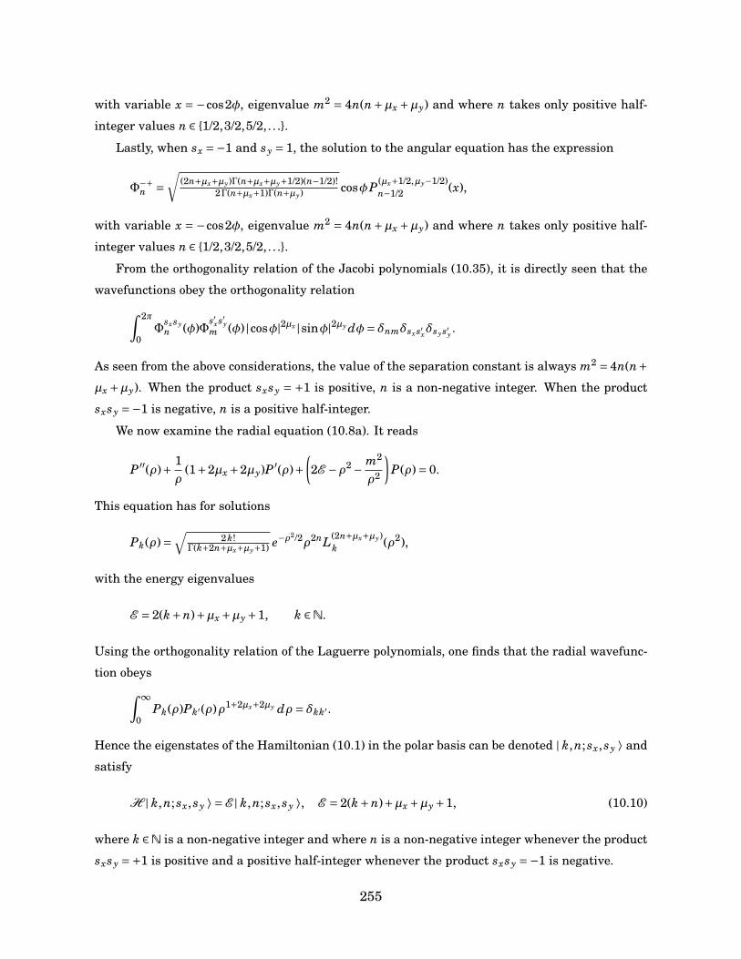
with variable x = −cos2φ, eigenvalue m2 = 4n(n+µx +µy) and where n takes only positive half-
integer values n ∈ 1/2,3/2,5/2, . . ..
Lastly, when sx =−1 and sy = 1, the solution to the angular equation has the expression
Φ−+n =
√(2n+µx+µy)Γ(n+µx+µy+1/2)(n−1/2)!
2Γ(n+µx+1)Γ(n+µy) cosφP(µx+1/2,µy−1/2)n−1/2 (x),
with variable x = −cos2φ, eigenvalue m2 = 4n(n+µx +µy) and where n takes only positive half-
integer values n ∈ 1/2,3/2,5/2, . . ..
From the orthogonality relation of the Jacobi polynomials (10.35), it is directly seen that the
wavefunctions obey the orthogonality relation∫ 2π
0Φ
sxsyn (φ)Φ
s′xs′ym (φ) |cosφ|2µx |sinφ|2µy dφ= δnmδsxs′xδsys′y .
As seen from the above considerations, the value of the separation constant is always m2 = 4n(n+µx +µy). When the product sxsy = +1 is positive, n is a non-negative integer. When the product
sxsy =−1 is negative, n is a positive half-integer.
We now examine the radial equation (10.8a). It reads
P ′′(ρ)+ 1ρ
(1+2µx +2µy)P ′(ρ)+(2E −ρ2 − m2
ρ2
)P(ρ)= 0.
This equation has for solutions
Pk(ρ)=√
2k!Γ(k+2n+µx+µy+1) e−ρ
2/2ρ2nL(2n+µx+µy)k (ρ2),
with the energy eigenvalues
E = 2(k+n)+µx +µy +1, k ∈N.
Using the orthogonality relation of the Laguerre polynomials, one finds that the radial wavefunc-
tion obeys∫ ∞
0Pk(ρ)Pk′(ρ)ρ1+2µx+2µy dρ = δkk′ .
Hence the eigenstates of the Hamiltonian (10.1) in the polar basis can be denoted | k,n; sx, sy ⟩ and
satisfy
H | k,n; sx, sy ⟩ = E | k,n; sx, sy ⟩, E = 2(k+n)+µx +µy +1, (10.10)
where k ∈N is a non-negative integer and where n is a non-negative integer whenever the product
sxsy =+1 is positive and a positive half-integer whenever the product sxsy =−1 is negative.
255
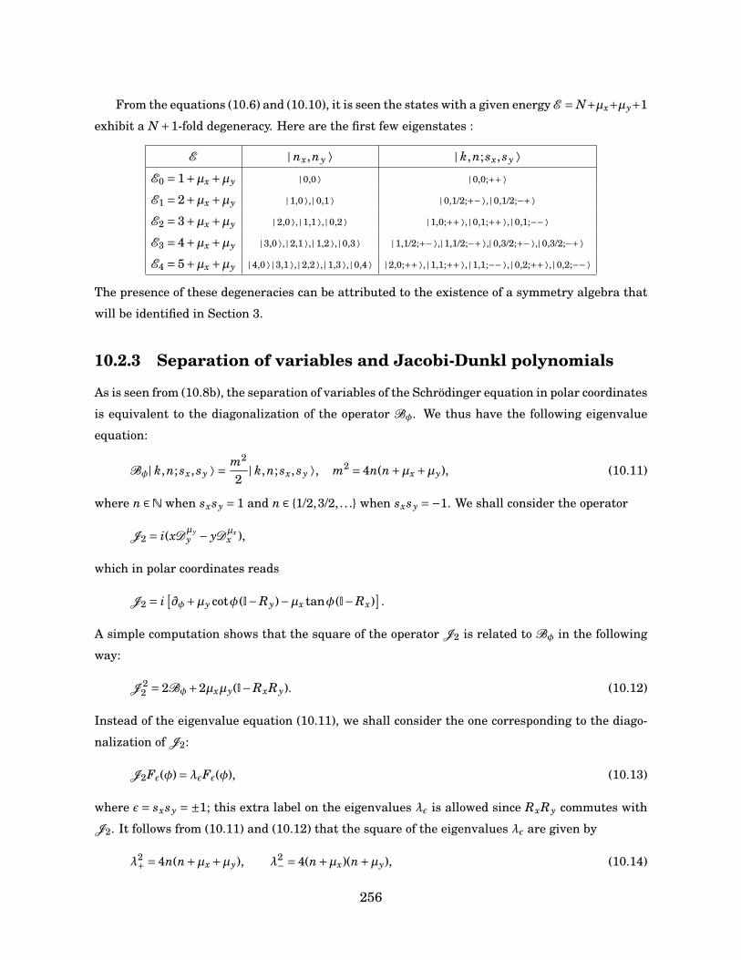
From the equations (10.6) and (10.10), it is seen the states with a given energy E = N+µx+µy+1
exhibit a N +1-fold degeneracy. Here are the first few eigenstates :
E | nx,ny ⟩ | k,n; sx, sy ⟩E0 = 1+µx +µy | 0,0 ⟩ | 0,0;++ ⟩
E1 = 2+µx +µy | 1,0 ⟩, | 0,1 ⟩ | 0,1/2;+− ⟩, | 0,1/2;−+ ⟩
E2 = 3+µx +µy | 2,0 ⟩, | 1,1 ⟩, | 0,2 ⟩ | 1,0;++ ⟩, | 0,1;++ ⟩, | 0,1;−− ⟩
E3 = 4+µx +µy | 3,0 ⟩, | 2,1 ⟩, | 1,2 ⟩, | 0,3 ⟩ | 1,1/2;+− ⟩,| 1,1/2;−+ ⟩,| 0,3/2;+− ⟩,| 0,3/2;−+ ⟩
E4 = 5+µx +µy | 4,0 ⟩ | 3,1 ⟩, | 2,2 ⟩, | 1,3 ⟩, | 0,4 ⟩ | 2,0;++ ⟩, | 1,1;++ ⟩, | 1,1;−− ⟩, | 0,2;++ ⟩, | 0,2;−− ⟩
The presence of these degeneracies can be attributed to the existence of a symmetry algebra that
will be identified in Section 3.
10.2.3 Separation of variables and Jacobi-Dunkl polynomials
As is seen from (10.8b), the separation of variables of the Schrödinger equation in polar coordinates
is equivalent to the diagonalization of the operator Bφ. We thus have the following eigenvalue
equation:
Bφ| k,n; sx, sy ⟩ = m2
2| k,n; sx, sy ⟩, m2 = 4n(n+µx +µy), (10.11)
where n ∈N when sxsy = 1 and n ∈ 1/2,3/2, . . . when sxsy =−1. We shall consider the operator
J2 = i(xDµyy − yD
µxx ),
which in polar coordinates reads
J2 = i[∂φ+µy cotφ (I−Ry)−µx tanφ (I−Rx)
].
A simple computation shows that the square of the operator J2 is related to Bφ in the following
way:
J 22 = 2Bφ+2µxµy(I−RxRy). (10.12)
Instead of the eigenvalue equation (10.11), we shall consider the one corresponding to the diago-
nalization of J2:
J2Fε(φ)=λεFε(φ), (10.13)
where ε= sxsy =±1; this extra label on the eigenvalues λε is allowed since RxRy commutes with
J2. It follows from (10.11) and (10.12) that the square of the eigenvalues λε are given by
λ2+ = 4n(n+µx +µy), λ2
− = 4(n+µx)(n+µy), (10.14)
256

where n ∈ N when ε = 1 and n = 1/2,3/2, . . . when ε = −1. Moreover, since sxsy = ε, we have
Rx = εRy. To solve (10.13), we consider the decomposition
Fε(φ)= f +ε (φ)+ f −ε (φ), (10.15)
where Ry f ±ε (φ) = ± f ±ε (φ). It is directly seen that given the decomposition (10.15), the eigenvalue
equation (10.13) is equivalent to the system of differential equations
∂φ[f +ε + f −ε
]+2µy cotφ f −ε −µx tanφ [(1−ε) f +ε + (1+ε) f −ε ]=−iλε[ f +ε + f −ε ],
∂φ[− f +ε + f −ε
]+2µy cotφ f −ε −µx tanφ [(ε−1) f +ε + (1+ε) f −ε ]=−iλε[ f +ε − f −ε ],
where the second equation was obtained from the first one by applying Ry. These equa-
tions are easily seen to be equivalent to
∂φ f −ε +2µy cotφ f −ε −µx tanφ(1+ε) f −ε =−iλε f +ε ,
∂φ f +ε −µx tanφ (1−ε) f +ε =−iλε f −ε .
The case ε= 1
When ε=+1, one has
∂φ f −+ +2µy cotφ f −+ −2µx tanφ f −+ =−iλ+ f ++ (10.16a)
∂φ f ++ =−iλ+ f −+ , (10.16b)
Substituting (10.16b) in (10.16a) yields the equation
∂2φ f ++ + (2µy cotφ−2µx tanφ)∂φ f ++ +λ2
+ f ++ = 0.
Since λ2+ = 4n(n+µx +µy), we directly obtain the result
f ++ = P (µx−1/2,µy−1/2)n (x), f −+ = i
λ+∂φ f ++ ,
with x =−cos2φ, eigenvalues λ+ =±2√
n(n+µx +µy) and n ∈N. Consequently, for ε=+,
the eigensolutions of (10.12) are given by
F+(φ)= P (α,β)n (x)+ i
λ+∂φP (α,β)
n (x), (10.17)
where the eigenvalues are given by
λ+ =±2√
n(n+µx +µy), n ∈N,
257
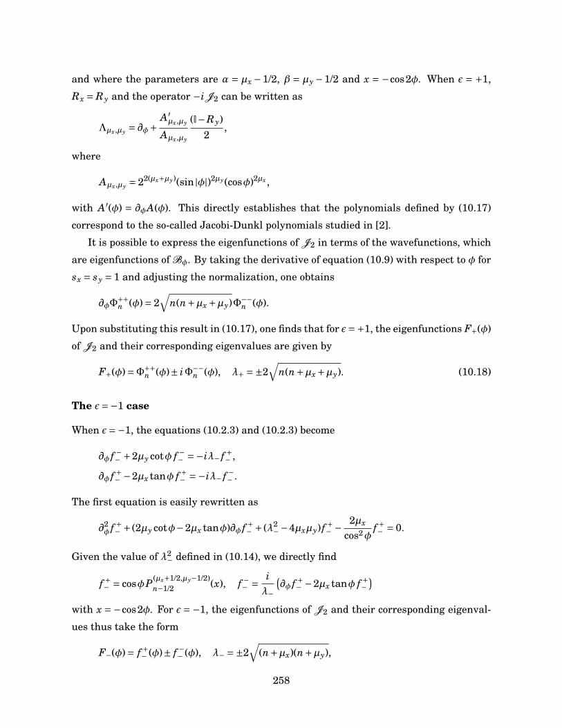
and where the parameters are α = µx −1/2, β = µy −1/2 and x = −cos2φ. When ε = +1,
Rx = Ry and the operator −iJ2 can be written as
Λµx,µy = ∂φ+A′µx,µy
Aµx,µy
(I−Ry)2
,
where
Aµx,µy = 22(µx+µy)(sin |φ|)2µy(cosφ)2µx ,
with A′(φ) = ∂φA(φ). This directly establishes that the polynomials defined by (10.17)
correspond to the so-called Jacobi-Dunkl polynomials studied in [2].
It is possible to express the eigenfunctions of J2 in terms of the wavefunctions, which
are eigenfunctions of Bφ. By taking the derivative of equation (10.9) with respect to φ for
sx = sy = 1 and adjusting the normalization, one obtains
∂φΦ++n (φ)= 2
√n(n+µx +µy)Φ−−
n (φ).
Upon substituting this result in (10.17), one finds that for ε=+1, the eigenfunctions F+(φ)
of J2 and their corresponding eigenvalues are given by
F+(φ)=Φ++n (φ)± iΦ−−
n (φ), λ+ =±2√
n(n+µx +µy). (10.18)
The ε=−1 case
When ε=−1, the equations (10.2.3) and (10.2.3) become
∂φ f −− +2µy cotφ f −− =−iλ− f +− ,
∂φ f +− −2µx tanφ f +− =−iλ− f −− .
The first equation is easily rewritten as
∂2φ f +− + (2µy cotφ−2µx tanφ)∂φ f +− + (λ2
−−4µxµy) f +− − 2µx
cos2φf +− = 0.
Given the value of λ2− defined in (10.14), we directly find
f +− = cosφP (µx+1/2,µy−1/2)n−1/2 (x), f −− = i
λ−
(∂φ f +− −2µx tanφ f +−
)with x =−cos2φ. For ε=−1, the eigenfunctions of J2 and their corresponding eigenval-
ues thus take the form
F−(φ)= f +− (φ)± f −− (φ), λ− =±2√
(n+µx)(n+µy),
258
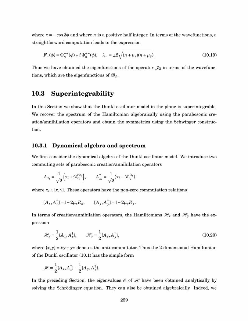
where x =−cos2φ and where n is a positive half integer. In terms of the wavefunctions, a
straightforward computation leads to the expression
F−(φ)=Φ−+n (φ)∓ iΦ+−
n (φ), λ− =±2√
(n+µx)(n+µy). (10.19)
Thus we have obtained the eigenfunctions of the operator J2 in terms of the wavefunc-
tions, which are the eigenfunctions of Bφ.
10.3 Superintegrability
In this Section we show that the Dunkl oscillator model in the plane is superintegrable.
We recover the spectrum of the Hamiltonian algebraically using the parabosonic cre-
ation/annihilation operators and obtain the symmetries using the Schwinger construc-
tion.
10.3.1 Dynamical algebra and spectrum
We first consider the dynamical algebra of the Dunkl oscillator model. We introduce two
commuting sets of parabosonic creation/annihilation operators
Axi =1p2
(xi +D
µxixi
), A†
xi= 1p
2(xi −D
µxixi ),
where xi ∈ x, y. These operators have the non-zero commutation relations
[Ax, A†x]= I+2µxRx, [A y, A†
y]= I+2µyRy.
In terms of creation/annihilation operators, the Hamiltonians Hx and H y have the ex-
pression
Hx = 12
Ax, A†x, H y = 1
2A y, A†
y, (10.20)
where x, y= xy+ yx denotes the anti-commutator. Thus the 2-dimensional Hamiltonian
of the Dunkl oscillator (10.1) has the simple form
H = 12
Ax, A†x+ 1
2A y, A†
y.
In the preceding Section, the eigenvalues E of H have been obtained analytically by
solving the Schrödinger equation. They can also be obtained algebraically. Indeed, we
259
have the additional commutation relations
[Hxi , Axi ]=−Axi , [Hxi , A†xi
]= A†xi
(10.21a)
Axi ,Rxi = A†xi
,Rxi = 0, [Hxi ,Rxi ]= 0, (10.21b)
where xi ∈ x, y. It is easily seen from the relations (10.20), (10.21a) and (10.21b) that the
operators Hxi , Axi , A†xi and Rxi realize two independent copies of the parabosonic algebra
which we have related to sl−1(2) in [40]. It follows directly from the above commutation
relations that
Ex = nx +µx +1/2, E y = ny +µy +1/2, nx,ny ∈N.
A direct computation shows that the action of the ladder operators Ax, A†x on the Carte-
sian eigenbasis | nx,ny ⟩ is given by
A†x| nx,ny ⟩ =
√[nx +1]µx | nx +1,ny ⟩, Ax| nx,ny ⟩ =
√[nx]µx | nx −1,ny ⟩, (10.22)
and that of the reflection Rx by
Rx| nx,ny ⟩ = (−1)nx | nx,ny ⟩,
where [n]µ denotes the ’mu-numbers’:
[n]µ = n+µ(1− (−1)n).
Analogous formulas hold for the action of A y, A†y and Ry.
As noted previously, the spectrum of the Hamiltonian H has the form
EN = N +µx +µy +1, N ∈N,
and exhibits a N+1-fold ’accidental’ degeneracy at level N. These degeneracies will be ex-
plained in terms of the irreducible representations of the symmetry algebra of the Dunkl
oscillator.
10.3.2 Superintegrability and the Schwinger-Dunkl algebra
We now exhibit the symmetries of the Hamiltonian (10.1). Let us consider the operator
J3 = 14
Ax, A†x− 1
4A y, A†
y= 12
(Hx −H y
).
260
It is clear that [H , J3] = 0 and that J3 is the symmetry corresponding to separation of
variables in Cartesian coordinates. Following the Schwinger construction [36], we further
introduce
J2 = 12i
(A†
x A y − Ax A†y
).
A direct computation shows that J2 is also a symmetry, i.e. [H , J2] = 0. In addition,
expressing the operator J2 in terms of Dunkl derivatives shows that
J2 = 12i
(xD
µxy − yD
µxx
),
and hence J2 =−J2/2; it is thus seen from (10.12) that J2 is associated to the separation
of variables in polar coordinates. To obtain the complete symmetry algebra, we define a
third operator which also commutes with H :
J1 = 12
(A†
x A y + Ax A†y
).
A direct computation show that the symmetry operators of the Dunkl oscillator in the
plane satisfy the following algebra
J1,Rxi = 0, J2,Rxi = 0, [J3,Rxi ]= 0,
[J2, J3]= iJ1, [J3, J1]= iJ2,
[J1, J2]= i[J3 + J3 (µxRx +µyRy)−H (µxRx −µyRy)/2
],
with R2x = R2
y = I, xi ∈ x, y and where the Hamiltonian H is a central element. We shall
refer to the algebra generated by J1, J2, J3, Rx, Ry and H as the Schwinger-Dunkl
algebra sd(2); special cases of it have appeared in other contexts [9, 14]. It is easily seen
that sd(2) is a deformation of the Lie algebra u(2) by the two involutions Rx, Ry. The
Schwinger-Dunkl algebra admits the Casimir operator [9]
C = J21 + J2
2 + J23 + 1
2µxRx + 1
2µyRy +µxµyRxRy,
which commutes with all the generators. A direct computation shows that in the present
realization, the Casimir operator C takes the value
C = 14
H 2 − 14
.
Since H is a central element, we can define
C = C−H 2/4+1/4,
261
and thus C = 0 in this realization.
The irreducible representations of the Schwinger-Dunkl algebra sd(2) can be used to
account for the degeneracies of the Hamiltonian (10.1). We shall postpone this study
for the second paper of the present series. Note that upon taking µx = µy = 0 in the
Schwinger-Dunkl algebra, the involutions cease to play an essential role and one recovers
the well-known su(2) symmetry algebra of the standard quantum harmonic oscillator in
the plane.
10.4 Overlap Coefficients
In this section, we obtain the expansion (overlap) coefficients between the Cartesian and
polar bases. These expansion coefficients are denoted by ⟨ k,n; sx, sy | nx,ny ⟩. It is clear
that the coefficients will vanish unless the involved states | k,n; sx, sy ⟩ and | nx,ny ⟩ belong
to the same energy eigenspace. The states in the polar basis are the eigenstates of the
operator Bφ given in (10.7) and satisfy
Bφ| k;n; sx, sy ⟩ = γn| k,n; sx, sy ⟩, γn = 2n(n+µx +µy),
with n a non-negative integer whenever the product sxsy = 1 and a positive half-integer
otherwise. We can consider the relation
γn⟨ k,n; sx, sy | nx,ny ⟩ = ⟨ k,n; sx, sy |Bφ | nx,ny ⟩,
and expand the action of Bφ on the Cartesian basis to obtain a recursion relation for
the overlap coefficients. It will prove more convenient to investigate first the overlap
coefficients between the Cartesian basis and the eigenbasis of a new operator Q related
to J2. The eigenstates of this new operator Q will then be expanded in terms of the polar
basis | k,n; sx, sy ⟩ to obtain the desired result. For this part, it is convenient to separate
the two eigenvalue sectors corresponding to the value of the product sxsy =±1.
10.4.1 Overlap coefficients for sxsy =+1
We start by expressing the energy eigenstates in the polar basis in terms of the eigen-
states of J2. As is seen from (10.18), the eigenvectors of the operator J2 with eigenvalues
262
κ±n that we denote | n,++ ⟩J2 and | n,+− ⟩J2 are given by
| n,++ ⟩J2 =1p2
(| k;n;++ ⟩+ i| k,n;−− ⟩
), κ+n = 2
√n(n+µx +µy),
| n,+− ⟩J2 =1p2
(| k;n;++ ⟩− i| k,n;−− ⟩
), κ−n =−2
√n(n+µx +µy),
for n 6= 0. For n = 0, one has
| 0,++ ⟩J2 =| k,0;++ ⟩, κ+0 = 0.
We also recall that Ry| n,++ ⟩J2 =| n,+− ⟩J2 . We now introduce the operator Q defined by
Q = iJ2Rx −µxRy −µyRx − (1/2)RxRy. (10.23)
The relevance of the operator Q will become clear in Section 5 when the connection be-
tween the Schwinger-Dunkl algebra and the Clebsch-Gordan problem of sl−1(2) will be
established. In the sector sxsy =+1, we have Rx = Ry and Q may be written as
Q = iJ2Ry −µxRy −µyRy − (1/2)I.
For n 6= 0, the eigenvalues q±n and eigenvectors | n,+± ⟩Q of Q are found to be
| n,++ ⟩Q = 1p2
(ζn| n,++ ⟩J2+| n,+− ⟩J2
), q+
n =−2n−µx −µy −1/2,
and
| n,+− ⟩Q = 1p2
(−ζn| n,++ ⟩J2+| n,+− ⟩J2
), q−
n = 2n+µx +µy −1/2,
where we have defined
ζn =[µx +µy −2i
√n(n+µx +µy)
2n+µx +µy
].
This amounts to the diagonalization of a 2×2 matrix. We note that ζnζ∗n = 1. When n = 0,
one has directly
| 0,++ ⟩Q =| 0,++ ⟩J2 , q+0 =−µx −µy −1/2.
It is possible to regroup the eigenvalues of Q into a single expression. We have
q` = (−1)`+1(`+µx +µy +1/2),
263
and the eigenvectors are given by
| q2 j ⟩Q = 1p2
(ζ j | j,++ ⟩J2 + (1−δ j0)| j,+− ⟩J2
),
| q2 j+1 ⟩Q = 1p2
(−ζ j+1 | j+1,++ ⟩J2+| j+1,+− ⟩J2
).
In the previous formulas, it should be understood that for the vector | q0 ⟩ the normaliza-
tion factorp
2 is not needed.
Having introduced the operator Q, we examine the overlap coefficients between its
eigenstates and the eigenstates of H in the Cartesian basis for a given energy level EN .
In the sector sxsy =+1, the possible levels take the energy values
EN = N +µx +µy +1,
where N is an even integer. The eigenspace EN is spanned by the vectors
| 0, N ⟩, | 1, N −1 ⟩, . . . , | m, N −m ⟩, . . . , | N,0 ⟩.
We shall denote the overlap coefficients by
⟨ q` | m, N −m ⟩ = M`m,N .
To obtain the expression for the expansion coefficients M`m,N , we start from the relation
q` M`m,N = ⟨ q` |Q | m, N −m ⟩. (10.24)
In terms of the parabosonic creation/annihilation operators, the operator Q reads
Q = (Ax A†y − A†
x A y)Rx − (µx +µy)Rx − (1/2)I. (10.25)
Upon substituting (10.25) in (10.24) and using the actions (10.22), there comes
q` M`m,N = Am+1 M`
m+1,N +Bm M`m,N + Am M`
m−1,N ,
where
Am = (−1)m√
[m]µx[N −m+1]µy , Bm = (−1)m+1(µx +µy)−1/2.
It follows that the overlap coefficients M`m,N can be expressed in terms of polynomials
Pm(q`). Indeed, if we define
M`m,N = M`
0,N Pm(q`),
264
with P0(q`)= 1, it transpires that Pm(q`) are polynomials of degree m in the variable q`obeying the three-term recurrence relation
q`Pm(q`)= Am+1Pm+1(q`)+BmPm(q`)+ AmPm−1(q`). (10.26)
Upon introducing the monic polynomials Pm(q`):
Pm(q`)= Pm(q`)A1 · · ·Am
,
the recurrence relation (10.26) becomes
q` Pm(q`)= Pm+1(q`)+BmPm(q`)+UmPm−1(q`), (10.27)
where
Un = A2n = [m]µx[N −m+1]µy . (10.28)
Comparing the formulas (10.27) and (10.28) with the formula (10.36) of Appendix A, it
is seen that the polynomials Pm(q`) correspond to the monic dual −1 Hahn polynomials
Qn(x`;α,β; N). We thus have
Pm(q`)= 2−mQm(x`,α,β; N)
where the parameter identification is given by
α= 2µy +N +1, β= 2µx +N +1,
and the variable x` takes the values
x` = (−1)`+1(2`+2µx +2µy +1), `= 0, . . . , N.
The value of M`0,N can be obtained from the requirement that the overlap coefficients
provide a unitary transformation between the two bases. Using the orthogonality relation
(10.37) of the dual −1 Hahn polynomials, we obtain
⟨ q` | m, N −m ⟩ =√
ωN−`U1 · · ·Um
Qm(x`;α,β; N),
where ωN−` is the weight function (10.38) of the dual −1 Hahn polynomials and N is
an even integer. It is seen from the formula (10.38) of Appendix A that if µx > −1/2
265
and µy > −1/2, the weight function ωN−` is positive for all ` ∈ 0, . . . , N. The overlap
coefficients obey the orthonormality relation
N∑`=0
⟨ q` | m, N −m ⟩⟨ n, N −n | q` ⟩ = δnm.
It now possible to obtain the overlap coefficients between the Cartesian and polar
wavefunctions of the Dunkl oscillator. We first observe that the eigenstates of Q have the
expansion
| q2n+p ⟩ =[
1+(−1)pζn+p2
]| k,n+ p ;++ ⟩+
[1−(−1)pζn+p
2i
]| k,n+ p ;−− ⟩,
with p = 0,1; the formula is also valid for n = p = 0. The inverse relations have the explicit
form
| k,n;++ ⟩=[ζn −1ζn
]| q2n−1 ⟩−
[ζn +12iζn
]| q2n ⟩,
| k,n;−− ⟩=[ζn +1ζn
]| q2n−1 ⟩+
[1−ζn
2iζn
]| q2n ⟩,
for n 6= 0. These formulas can be used directly to obtain the overlap coefficients
⟨ k,n;++ | m, N −m ⟩, ⟨ k,n;−− | m, N −m ⟩,
as linear combinations of dual −1 Hahn polynomials.
10.4.2 Overlap coefficients for sxsy =−1
The overlap coefficients in the parity sector sxsy = −1 are obtained similarly to the case
sxsy = 1. We again start by writing the energy eigenstates in the polar basis in terms of
the eigenstates of the operator J2. It follows from the relation (10.19) that the eigenstates
of the operator J2 with eigenvalues σ±n that we denote by | n,−+ ⟩J2 and | n,−− ⟩J2 are
given by
| n,−+ ⟩J2 =1p2
(| k,n;−+ ⟩− i| k,n;+− ⟩
), σ+
n = 2√
(n+µx)(n+µy),
| n,−− ⟩J2 =1p2
(| k,n;−+ ⟩+ i| k,n;+− ⟩
), σ−
n =−2√
(n+µx)(n+µy),
where n ∈ 1/2, 3/2, . . .. In this sector, the operator Q is equivalent to
Q = iJ2Rx + (µx −µy)Rx + (1/2)I.
266
The eigenstates | n,−± ⟩Q and eigenvalues q±n of Q are easily found to be
| n,−+ ⟩Q = 1p2
(ξn| n,−+ ⟩J2+| n,−− ⟩J2
), q+
n = 1/2−2n−µx −µy,
and
| n,−− ⟩Q = 1p2
(−ξn| n,−+ ⟩J2+| n,−− ⟩J2
), q−
n = 1/2+2n+µx +µy,
where
ξn =[µx −µy +2i
√(n+µx)(n+µy)
2n+µx +µy
].
It is easily verified that ξnξ∗n = 1. The eigenstates of Q can be grouped in a single expres-
sion. We write
q` = (−1)`+1(`+µx +µy +1/2).
The eigenvectors have the expressions
| q2 j+p ⟩Q = 1p2
((−1)pξ j+1/2 | j+1/2,−+ ⟩J2+| j+1/2,−− ⟩J2
).
We now compute the overlap coefficients between the eigenstates of Q and the eigen-
states of H expressed in the Cartesian basis for a given energy level EN . In the sector
sxsy =−1, the energy takes the values
EN = N +µx +µy +1,
where N is an odd integer. The eigenspace corresponding to EN is spanned by the vectors
| 0, N ⟩, | 1, N −1 ⟩, · · ·| m, N −m ⟩, · · · , | N,0 ⟩.
We denote the overlap coefficients by
⟨ q` | m, N −m ⟩ =W`m,N .
The coefficients W`m,N can be computed from the relation
q` ⟨ q` | m, N −m ⟩ = ⟨ q` |Q | m, N −m ⟩. (10.29)
In terms of the parabosonic operators, the operator Q acting on the sector sxsy reads
Q = (Ax A†y − A†
x A y)Rx + (µx −µy)Rx + (1/2)I. (10.30)
267
Upon substituting (10.30) in (10.29) and using the actions (10.22), one finds the recurrence
relation
q`W`m,N = Am+1 W`
m+1,N + Bm W`m,N + Am W`
m−1,N ,
where
Am = (−1)m√
[m]µx[N −m+1]µy , Bm = (−1)m(µx −µy)+1/2.
After writing
W`m,N =W`
0,N Pm(q`),
with P0(q`)= 1 and introducing the monic polynomials
Pm(q`)= Pm(q`)A1 · · ·Am
,
one finds that the polynomials Pm(q`) satisfy the three-term recurrence relation
q` Pm(q`)= Pm+1(q`)+ Bm Pm(q`)+UnPm−1(q`), (10.31)
with
Um = [m]µx[N −m+1]µy .
By comparing the recurrence relation (10.31) with that of the dual −1 Hahn polynomials
(10.36), one obtains
Pm(q`)= 2−mQm(x`,α,β, N),
with the parameter identification
α= 2µx, β= 2µy,
and the variable
x` = (−1)`(2`+2µx +2µy +1).
The requirement that the overlap coefficients provide a unitary transformation leads to
the relation
⟨ q` | m, N −m ⟩ =√
w`
U1 · · ·UmQm(x`,α,β, N),
268
where N is an odd integer. The overlap coefficients satisfy the orthogonality relation
N∑`=0
⟨ q` | m, N −m ⟩⟨ q` | n, N −n ⟩ = δnm.
It is again possible to recover the overlap coefficients between the wavefunctions by
expressing the eigenvectors of Q in terms of the eigenstates in the polar basis. One has
| q2 j+p ⟩ =[
1+(−1)pξ j+1/22
]| k, j+1/2;−+ ⟩+
[(−1)pξ j+1/2−1
2i
]| k,n;+− ⟩,
with p ∈ 0,1. The inverse relation reads
| k, j+1/2;−+ ⟩=[
1+ξ j+1/22ξ j+1/2
]| q2 j ⟩+
[ξ j+1/2−12iξ j+1/2
]| q2 j+1 ⟩,
| k, j+1/2;+− ⟩=[ξ j+1/2−12ξ j+1/2
]| q2 j ⟩+
[1+ξ j+1/22iξ j+1/2
]| q2 j+1 ⟩.
Hence it is seen that the expansion coefficients between the Cartesian and polar bases are
given in terms of linear combinations of dual −1 Hahn polynomials. These coefficients can
also be expressed in integral form using the separated wavefunctions obtained in Section
2.
10.5 The Schwinger-Dunkl algebra and the Clebsch-
Gordan problem
The Schwinger-Dunkl algebra and the dual −1 Hahn polynomials have both appeared in
the examination of the Clebsch-Gordan problem for the Hopf algebra sl−1(2) [9, 40]. In
this Section, we explain the relationship between the two contexts. This will clarify the
introduction of the operator Q in the previous Section.
10.5.1 sl−1(2) Clebsch–Gordan coefficients and
overlap coefficients
The sl−1(2) algebra is generated by the elements A0, A± and R with the defining relations
[A0,R]= 0, [A0, A±]=±A±, A±,R= 0, A+, A−= 2A0,
and R2 = I. It admits the Casimir operator
Q = A+A−R− A0R+ (1/2)R,
269
which commutes will all the generators. This algebra has infinite-dimensional irreducible
modules V (ε,µ) spanned by the basis vectors v(ε,µ)n , n ∈N. The action of the generators on
the basis vectors is
A0v(ε,µ)n = (n+µ+1/2)v(ε,µ)
n , Rv(ε,µ)n = ε(−1)nv(ε,µ)
n ,
A+v(ε,µ)n =
√[n+1]µv(ε,µ)
n+1 , A−v(ε,µ)n =
√[n]µv(ε,µ)
n−1 .
It is easily seen that Q v(ε,µ)n =−εµv(ε,µ)
n .
The sl−1(2) algebra is a Hopf algebra and has a non-trivial co-product. Upon taking
the tensor product of two irreducible modules V (ε1,µ1)⊗V (ε2,µ2) spanned by the basis vectors
e(ε1,µ1)n ⊗ e(ε2,µ2)
m , one obtains a third module V (in general not irreducible) by adjoining the
action
A0(v⊗w)= (A0v)⊗w+v⊗ (A0w), R(v⊗w)= (Rv)⊗ (Rw),
A±(v⊗w)= (A±v)⊗ (Rw)+v⊗ (A±w),
where v ∈V (ε1,µ1) and w ∈V (ε2,µ2). On V , we have the Casimir element
Q = (A(1)− A(2)
+ − A(1)+ A(2)
− )R(1) − (1/2)R(1)R(2) −ε1µ1R(2) −ε2µ2R(1),
where the superscripts indicate on which module the generators act; e.g. A(1)± = A±⊗ I.
The eigenvalues of Q represent the irreducible modules V (εi ,µi) appearing in the de-
composition of V =⊕i V (εiµi). The Clebsch-Gordan coefficients of sl−1(2) are the expansion
coefficients between the direct product basis e(ε1,µ1)n ⊗ e(ε2,µ2)
m and the eigenbasis f (ε1,µi)k of
the operator Q; this corresponds to the ’coupled’ basis. Given the addition rule of A0, one
has
f (ε1,µi)N = ∑
n1+n2=NCµ1µ2µi
n1n2N e(ε1,µ1)n1 ⊗ e(ε2,µ2)
n2 , (10.32)
where Cµ1µ2µin1n2N are the Clebsch-Gordan coefficients, which were shown to be given in terms
of dual −1 Hahn polynomials in [9, 40].
In our model, it is seen that the operators Hx, Ax, A†x, and H y, A y, A†
y realize the
two sl−1(2) modules Vµx and Vµy , with εx = εy = 1. The Cartesian basis states | nx,ny ⟩correspond to the direct product basis and the operator Q given in (10.23) corresponds to
the Casimir operator Q. This explains the origin of the operator Q in our approach to the
overlap coefficients.
270
10.5.2 Occurrence of the Schwinger-Dunkl algebra
In our model, the Schwinger-Dunkl algebra occurs as the symmetry algebra. The algebra
sd(2) also appears in the C.G. problem of sl−1(2) as a ’hidden’ algebra. We illustrate how
this comes about.
In the C.G. problem, it follows from (10.32) that the following operators act as multiple
of the identity:
A(1)0 + A(2)
0 , Q(1), Q(2), R(1)R(2). (10.33)
In the direct product basis, in addition to the operators (10.33), the operators
K0 = (A(1)0 − A(2)
0 )/2, R = R(1)
and R(2) are also diagonal. In the ’coupled’ basis, in addition to (10.33), we have the
Casimir operator K1 = Q which is diagonal. Hence, the tensor product basis corresponds
to having the operators (10.33) plus K0 and R in diagonal form and the coupled basis
corresponds to having the operators (10.33) and K1 in diagonal form. A direct computation
shows that the set K0, K1, R generates the Schwinger-Dunkl algebra [9].
We have thus established the connection between our model and the Clebsch-Gordan
problem of the algebra sl−1(2).
10.6 Conclusion
We considered the Dunkl oscillator model and showed that it is a superintegrable system.
We have exhibited the symmetry algebra that we called the Schwinger-Dunkl algebra
and we have obtained the exact solutions of the Schrödinger equation in terms of Jacobi,
Laguerre and generalized Hermite polynomials in Cartesian and polar coordinates. The
expansion coefficients between the Cartesian and polar bases have been obtained exactly
in terms of linear combinations of dual −1 Hahn polynomials and we established the con-
nection between these overlap coefficients and the Clebsch-Gordan problem of the algebra
sl−1(2).
The representations of the symmetry algebra of a superintegrable system explain how
the degenerate eigenstates of this system are transformed into each other. In the second
series of the paper, we shall consider the representations of the Schwinger-Dunkl alge-
bra. As will be seen, these representations exhibit remarkable occurrences of other −1
polynomials.
271
It would be of interest to consider in a future study the 3D Dunkl oscillator model,
which will provide another example of a superintegrable system with reflections. It was
shown in [10] that the Bannai–Ito polynomials occur as Racah coefficients of the algebra
sl−1(2). Given the connection between the 2D Dunkl oscillator and the Clecbsch-Gordan
problem of sl−1(2), one can expect that the Bannai–Ito polynomials will occur in the de-
scription of the 3D Dunkl oscillator model.
10.A Appendix A
10.A.1 Formulas for Laguerre polynomials
The Laguerre polynomials L(α)n (x) are defined by [23]:
L(α)n (x)= (α+1)n
n! 1F1
[ −nα+1
; x],
where (a)n = (a)(a+1) · · · (a+n−1) is the Pochhammer symbol. They obey the orthogonality
relation:∫ ∞
0e−xxαL(α)
m (x)L(α)n (x)= Γ(n+α+1)
n!δnm, (10.34)
for α>−1.
10.A.2 Formulas for Jacobi polynomials
The Jacobi polynomials P (α,β)n (x) are defined by [23]:
P (α,β)n (x)= (α+1)n
n! 2F1
[−n n+α+β+1α+1
;1− x
2
]They obey the orthogonality relation:∫ 1
−1(1− x)α(1+ x)βP (α,β)
m (x)P (α,β)n (x)= 2α+β+1
2n+α+β+1Γ(n+α+1)Γ(n+β+1)Γ(n+α+β+1)n! δnm, (10.35)
provided that α>−1 and β>−1.
10.A.3 Formulas for dual −1 Hahn polynomials
The monic dual −1 Hahn polynomials Qn(x;α,β; N) have the recurrence relation [41]:
xQn(x)=Qn+1(x)+bnQn(x)+unQn−1(x).
272

The recurrence coefficients are given by:
un = 4[n]ξ[N −n+1]ζ, bn =
(−1)n+1(2ξ+2ζ)−1, N even,
(−1)n(2ζ−2ξ)−1, N odd,, (10.36)
where
ξ=
β−N−1
2 , N even,α2 , N odd,
, ζ=
α−N−1
2 N even,β
2 , N odd.
They obey the orthogonality relation:
N∑`
ω`Qn(x`)Qm(x`)= vnδnm (10.37)
The weight is given by
ω2 j+q =
(−1) j(−m) j+q
j!(1−α/2) j(1−α/2−β/2) j
(1−β/2) j(m+1−α/2−β/2) j+q
(1−β/2)m(1−α/2−β/2)m
, N even,(−1) j(−m) j
j!(1/2+α/2) j+q(1/2+α/2+β/2) j
(1/2+β/2) j+q(m+3/2+α/2+β/2) j
(1/2+β/2)m+1/2(1+α/2+β/2)m+1/2
, N odd.(10.38)
where q ∈ 0,1 and with m = N/2, vn = u1 · · ·un. The grid points have the expression
x` =
(−1)`(2`+1−α−β), N even,
(−1)`(2`+1+α+β), N odd.
10.B Appendix B
We here indicate how it can be simply seen that the Dunkl derivative (10.2) is anti-Hermitian with respect to the scalar product (10.5). This is recorded for completenessand convenience. We need to check that
⟨ψ2 |Dµxψ1 ⟩ =
∫ ∞
−∞ψ∗
2 (x)[Dµxψ1(x)]|x|2µx dx =−
∫ ∞
−∞[Dµ
xψ2(x)]∗ψ1(x)|x|2µx dx =−⟨Dµxψ2 |ψ1 ⟩,
for all functions ψ1(x), ψ2(x) belonging to the L2 space associated to the scalar produt
(10.5). We split the computation in the four possible parity cases for ψ1(x), ψ2(x). This is
sufficient since any function can be decomposed into its even and odd parts and since the
scalar product (10.5) is linear in its arguments.
273
In the even-even case, one has ψ1(x)=ψ1(−x), ψ2(x)=ψ2(−x). It follows that
⟨ψ2 |Dµxψ1 ⟩ =
∫ ∞
−∞ψ∗
2 (x)[Dµxψ1(x)]|x|2µdx =
∫ ∞
−∞ψ∗
2 (x)[∂xψ1(x)]|x|2µdx = 0,
since the integrand in odd. Similarly, we have ⟨Dµxψ2 |ψ1 ⟩ = 0.
In the odd-odd case ψ1(x)=−ψ1(−x), ψ2(x)=−ψ2(−x) and one obtains∫ ∞
−∞ψ∗
2 (x)[Dµxψ1(x)]|x|2µdx =
∫ ∞
−∞ψ∗
2 (x)[∂xψ1(x)+ 2µ
xψ1(x)
]|x|2µdx = 0,
since the integrand is odd. Similarly, we have ⟨Dµxψ2 |ψ1 ⟩ = 0.
In the even-odd case, ψ1(x)=−ψ1(−x), ψ2(x)=ψ2(−x) and it follows that∫ ∞
−∞ψ∗
2 (x)[Dµxψ1(x)]|x|2µdx =
∫ ∞
−∞ψ∗
2 (x)[∂xψ1(x)+ 2µ
xψ1(x)
]|x|2µdx
= 2∫ ∞
0ψ∗
2 (x)[∂xψ1(x)+ 2µ
xψ1(x)
]x2µdx
= 2ψ1(x)ψ∗2 (x)x2µ
∣∣∣∞0−2
∫ ∞
0∂x[ψ∗
2 (x)x2µ]ψ1(x)dx+4µ∫ ∞
0ψ∗
2 (x)ψ1(x)x2µ−1dx
=−2∫ ∞
0[∂xψ
∗2 (x)]ψ1(x)|x|2µdx =−
∫ ∞
−∞[Dµ
xψ2(x)]∗ψ1(x)|x|2µdx,
where we have used the vanishing conditions on ψ1(x), ψ2(x) at infinity. It thus seen that
⟨ψ2 |Dµxψ1 ⟩ =−⟨D
µxψ2 |ψ1 ⟩.
In the even-odd case, one has ψ1(x)=ψ1(−x), ψ2(x)=−ψ2(−x) and one obtains∫ ∞
−∞ψ∗
2 (x)[Dµxψ1(x)]|x|2µdx =
∫ ∞
−∞ψ∗
2 (x)[∂xψ1(x)]|x|2µdx = 2∫ ∞
0ψ∗
2 (x)[∂xψ1(x)] x2µdx
= 2ψ1(x)ψ∗2 (x)x2µ
∣∣∣∞0−2
∫ ∞
0
[∂xψ
∗2 (x)+ 2µ
xψ∗
2 (x)]ψ1(x) x2µdx
=−∫ ∞
−∞[Dµ
xψ2(x)]∗ψ1(x)|x|2µdx,
where we have used the vanishing conditions on ψ1(x), ψ2(x) at infinity. Hence we have
⟨ψ2 |Dµxψ1 ⟩ =−⟨D
µxψ2 |ψ1 ⟩ and the result
⟨ψ2 |Dµxψ1 ⟩ =−⟨D
µxψ2 |ψ1 ⟩.
is established in all cases.
References
[1] T. Chihara. An Introduction to Orthogonal Polynomials. Gordon and Breach, New-York,
1978.
274
[2] F. Chouchene. Harmonic analysis associated with the Jacobi-Dunkl operator on ]−π/2,π/2[.
Journal of Computational and Applied Mathematics, 178:75–89, 2005.
[3] K. Coulembier, H. De Bie, and F. Sommen. Orthogonality of the Hermite polynomials in
superspace and Mehler type formulae. Proceedings of the London Mathematica Society,
103:786–825, 2011.
[4] C. Daskaloyannis. Quadratic Poisson algebras and two-dimensional classical superintegrable
systems and quadratic associative algebras of quantum superintegrable systems. Journal of
Mathematical Physics, 42:1100–1119, 2001.
[5] H. De Bie, B. Orsted, P. Somberg, and V. Soucek. Dunkl operators and a family of realizations
of osp(1|2). Transactions of the American Mathematical Society, 364:3875–3902, 2012.
[6] C.F. Dunkl. Symmetric and BN -invariant spherical harmonics. Journal of Physics A: Mathe-
matical and Theoretical, 35:10391–10408, 2002.
[7] C.F. Dunkl. Dunkl operators and related special functions. ArXiv, 1210.3010, 2012.
[8] V. X. Genest, L. Vinet, and A. Zhedanov. Bispectrality of the Complementary Bannai-Ito
polynomials. SIGMA, 9:18, 2013.
[9] V. X. Genest, L. Vinet, and A. Zhedanov. The algebra of dual −1 Hahn polynomials and the
Clebsch-Gordan problem of sl−1(2). Journal of Mathematical Physics, 54:023506, 2013.
[10] V.X. Genest, L. Vinet, and A. Zhedanov. The Bannai-Ito polynomials as Racah coefficients of
the sl−1(2) algebra. Proceedings of the American Mathematical Society, 1422013.
[11] Y. Granovskii, A. Zhedanov, and I. Lutsenko. Mutual integrability, quadratic algebras and
dynamical symmetry. Annals of Physics, 217:1–20, 1992.
[12] Y. Granovskii, A. Zhedanov, and I. Lutsenko. Quadratic algebras and dynamics in curved
spaces I. Oscillator. Theoretical and Mathematical Physics, 91:474–480, 1992.
[13] Y. Granovskii, A. Zhedanov, and I. Lutsenko. Quadratic algebras and dynamics in curved
spaces II. The Kepler problem. Theoretical and Mathematical Physics, 91:604–612, 1992.
[14] E.I. Jafarov, N.I. Stoilova, and J. Van der Jeugt. The su(2)α Hahn oscillator and a discrete
Hahn-Fourier transform. Journal of Physics A: Mathematical and Theoretical, 44:355205,
2011.
[15] E.I. Jafarov, N.I. Stoilova, and J. Van der Jeugt. Deformed su(1,1) algebra as a model for
Quantum Oscillators. SIGMA, 8:025, 2012.
275
[16] E.G. Kalnins, J.M. Kress, and W. Jr. Miller. Second order superintegrable systems in con-
formally flat spaces. I. 2D classical structure theory. Journal of Mathematical Physics,
46:053509, 2005.
[17] E.G. Kalnins, J.M. Kress, and W. Jr. Miller. Second order superintegrable systems in confor-
mally flat spaces. II. The classical 2D Stäckel transform. Journal of Mathematical Physics,
46:053510, 2005.
[18] E.G. Kalnins, J.M. Kress, and W. Jr. Miller. Second order superintegrable systems in con-
formally flat spaces. III. 3D classical structure theory. Journal of Mathematical Physics,
46:103507, 2005.
[19] E.G. Kalnins, J.M. Kress, and W. Jr. Miller. Second order superintegrable systems in confor-
mally flat spaces. IV. The classical 3D Stäckel transform and 3D classification theory. Journal
of Mathematical Physics, 47:043514, 2006.
[20] E.G. Kalnins, J.M. Kress, and W. Jr. Miller. Second order superintegrable systems in con-
formally flat spaces. V. 2D and 3D quantum systems. Journal of Mathematical Physics,
46:093501, 2006.
[21] E.G. Kalnins, J.M. Kress, W. Jr. Miller, and G.S. Pogosyan. Completeness of superintegrabil-
ity in two-dimensional constant curvature spaces. Journal of Physics A: Mathematical and
Theoretical, 34:4705–4720, 2001.
[22] E.G. Kalnins, W. Jr. Miller, and G.S. Pogosyan. Superintegrability and higher order constants
for classical and quantum systems. Physics of Atomic Nuclei, 74:914–918, 2011.
[23] R. Koekoek, P.A. Lesky, and R.F. Swarttouw. Hypergeometric orthogonal polynomials and
their q-analogues. Springer, 1st edition, 2010.
[24] P. Létourneau and L. Vinet. Superintegrable systems: polynomial algebras and quasi-exactly
solvable hamiltonians. Annals of Physics, 243:144–168, 1995.
[25] H. Miki, S. Post, L. Vinet, and A. Zhedanov. A superintegrable finite oscillator in two dimen-
sions with SU(2) symmetry. Journal of Physics A: Mathematical and Theoretical, 46:125207,
2013.
[26] N. Mukunda, E.C.G. Sudarshan, J.K. Sharma, and C.L. Mehta. Representations and proper-
ties of para-Bose oscillator operators I. Energy position and momentum eigenstates. Journal
of Mathematical Physics, 21:2386–2394, 1980.
276
[27] A. Nowak and K. Stempak. Imaginary powers of the Dunkl harmonic oscillator. SIGMA,
5:16–28, 2009.
[28] M.S. Plyushchay. R-deformed Heisenberg algebras. Modern Physics Letters A, 11:2953–2964,
1996.
[29] M.S. Plyushchay. Deformed Heisenberg algebra with reflection. Nuclear Physics B, 491:619–
634, 1997.
[30] S. Post, S. Tsujimoto, and L. Vinet. Families of superintegrable Hamiltonians con-
structed from exceptional polynomials. Journal of Physics A: Mathematical and Theoretical,
45:405202, 2012.
[31] S. Post, L. Vinet, and A. Zhedanov. An infinite family of superintegrable Hamiltonians with
reflection in the plane. Journal of Physics A: Mathematical and Theoretical, 44:505201, 2011.
[32] M. Rosenblum. Generalized Hermite polynomials and the Bose-like oscillator calculus. In
Operator Theory: Advances and Applications, 1994.
[33] M. Rösler. Generalized Hermite polynomials and the heat equation for Dunkl operators.
Communications in Mathematical Physics, 192:519–542, 1998.
[34] M. Rösler. Dunkl operators: theory and applications. In Lecture notes in Mathematics.
Springer, 2002.
[35] A. Ruffing. On q-deformations and Dunkl-deformations of harmonic oscillators. In H. Gaus-
terer, L. Pittner, and Harald Grosse, editors, Geometry and Quantum Physics, volume 543 of
Lecture Notes in Physics, pages 398–399. Springer Berlin Heidelberg, 2000.
[36] J. Schwinger. On angular momentum. In L.C. Biedenharn and H. van Dam, editors, Quantum
Theory of Angular Momentum. Academic, 1965.
[37] P. Tempesta, A.V. Turbiner, and P. Winternitz. Exact solvability of superintegrable systems.
Journal of Mathematical Physics, 42:4248, 2001.
[38] F. Tremblay, A. Turbiner, and P. Winternitz. An infinite family of solvable and inte-
grable quantum systems in the plane. Journal of Physics A: Mathematical and Theoretical,
42:242001, 2009.
[39] F. Tremblay, A. Turbiner, and P. Winternitz. Periodic orbits for an infinite family of classical
superintegrable systems. Journal of Physics A: Mathematical and Theoretical, 43:015202,
2010.
277

[40] S. Tsujimoto, L. Vinet, and A. Zhedanov. From slq(2) to a parabosonic Hopf algebra. SIGMA,
7:93–106, 2011.
[41] S. Tsujimoto, L. Vinet, and A. Zhedanov. Dual −1 Hahn polynomials: "classical" polynomials
beyond the Leonard duality. Proceedings of the American Mathematical Society, 141:959–
970, 2012.
[42] S. Tsujimoto, L. Vinet, and A. Zhedanov. Dunkl shift operators and Bannai-Ito polynomials.
Advances in Mathematics, 229:2123–2158, 2012.
[43] L. Vinet and A. Zhedanov. A Bochner theorem for Dunkl polynomials. SIGMA, 7:20–29, 2011.
[44] L. Vinet and A. Zhedanov. A ’missing’ family of classical orthogonal polynomials20. Journal
of Physics A: Mathematical and Theoretical, 44:085201, 2011.
[45] L. Vinet and A. Zhedanov. A limit q = −1 for the Big q-Jacobi polynomials. Transactions of
the American Mathematical Society, 364:5491–5507, 2012.
[46] L. Vinet and A. Zhedanov. Para-Krawtchouk polynomials on a bi-lattice and a quantum
spin chain with perfect state transfer. Journal of Physics A: Mathematical and Theoretical,
45:265304, 2012.
[47] A. Zhedanov. The Higgs algebra as a quantum deformation of SU(2). Modern Physics Letters
A, 7:507–512, 1992.
278
Chapitre 11
The Dunkl oscillator in the plane II :representations of the symmetryalgebra
V. X. Genest, M. E. H. Ismail, L. Vinet et A. Zhedanov (2014). The Dunkl oscillator in the plane
II : representations of the symmetry algebra. Communications in Mathematical Physics 329 999–
1029
Abstract. The superintegrability, wavefunctions and overlap coefficients of the Dunkl oscillator
model in the plane were considered in the first part. Here finite-dimensional representations of
the symmetry algebra of the system, called the Schwinger-Dunkl algebra sd(2), are investigated.
The algebra sd(2) has six generators, including two involutions and a central element, and can
be seen as a deformation of the Lie algebra u(2). Two of the symmetry generators, J3 and J2, are
respectively associated to the separation of variables in Cartesian and polar coordinates. Using
the parabosonic creation/annihilation operators, two bases for the representations of sd(2), the
Cartesian and circular bases, are constructed. In the Cartesian basis, the operator J3 is diagonal
and the operator J2 acts in a tridiagonal fashion. In the circular basis, the operator J2 is block
upper-triangular with all blocks 2×2 and the operator J3 acts in a tridiagonal fashion. The expan-
sion coefficients between the two bases are given by the Krawtchouk polynomials. In the general
case, the eigenvectors of J2 in the circular basis are generated by the Heun polynomials and their
components are expressed in terms of the para-Krawtchouk polynomials. In the fully isotropic
case, the eigenvectors of J2 are generated by little −1 Jacobi or ordinary Jacobi polynomials. The
basis in which the operator J2 is diagonal is considered. In this basis, the defining relations of the
Schwinger-Dunkl algebra imply that J3 acts in a block tridiagonal fashion with all blocks 2×2.
279
The matrix elements of J3 in this basis are given explicitly.
11.1 Introduction
This is the second part of this series concerned with the analysis of the isotropic Dunkl oscillator
model. In part I, the model has been shown to be superintegrable, the wavefunctions have been
obtained in Cartesian and polar coordinates and the overlap coefficients have been found [5]. In
the present work, the representations of the symmetry algebra of the model, called the Schwinger-
Dunkl algebra (see below), are investigated. As shall be seen, this study entails remarkable con-
nections with special functions such as the Heun, little −1 Jacobi and para-Krawtchouk polyno-
mials.
11.1.1 Superintegrability
One recalls that a quantum system defined by a Hamiltonian H in d dimensions is maximally su-
perintegrable if it admits 2d−1 algebraically independent symmetry generators Si that commute
with the Hamiltonian
[Si,H]= 0, 16 i 6 2d−1,
where one of the symmetries is the Hamiltonian itself, e.g. S1 ≡ H. Moreover, a superintegrable
system is said to be of order ` if ` is the maximal order of the symmetries Si in the momentum
variables.
11.1.2 The Dunkl oscillator model
The isotropic Dunkl oscillator model [2, 5, 11] in the plane is possibly the simplest two-dimensional
system described by a Hamiltonian involving reflections. It is second-order superintegrable and is
defined by the Hamiltonian [5]
H =−12
[(Dµx
x )2 + (Dµyy )2]+ 1
2[x2 + y2], (11.1)
where Dµxixi is the Dunkl derivative [4, 14]
Dµxixi = ∂xi +
µxi
xi(I−Rxi ), ∂xi =
∂
∂xi,
with I denoting the identity operator and Rxi , xi ∈ x, y, standing for the reflection operator with
respect to the xi = 0 axis. Hence the reflections Rx, Ry that appear in the Hamiltonian (11.1) have
280
the action
Rx f (x, y)= f (−x, y), Ry f (x, y)= f (x,−y),
and thus evidently R2xi= I. In connection with the nomenclature of the standard harmonic oscil-
lator, the model is called isotropic because the quadratic potential is SO(2) invariant. For the full
Hamiltonian (11.1) to have this symmetry requires of course that µx =µy.
The Schrödinger equation associated to H is separable in both Cartesian and polar coordi-
nates. The spectrum of energies E is given by
EN = N +µx +µy +1, N = nx +ny, (11.2)
where nx, ny are non-negative integers. The wavefunctions are well defined for the values µx,µy ∈(−1
2 ,∞); the case µx =µy = 0 corresponds to the standard quantum harmonic oscillator. It is easily
seen from (11.2) that the energy level EN exhibits a N +1-fold degeneracy.
11.1.3 Symmetries of the Dunkl oscillator
The symmetries of the Dunkl oscillator Hamiltonian (11.1) can be obtained by the Schwinger
construction using the parabosonic creation/annihilation operators [5, 8, 10]. We consider the
operators [14, 15]
Axi± = 1p
2(xi ∓D
µxixi ), xi ∈ x, y. (11.3)
It is verified that the operators Axi± satisfy the following commutation relations:
[Axi− , Axi+ ]= I+2µxi Rxi , Axi± ,Rxi = 0, (11.4)
where x, y= xy+yx denotes the anticommutator. In addition to the commutation relations (11.4),
one has
[Axi± , Ax j
± ]= [Axi± ,Rx j ]= [Rxi ,Rx j ]= 0, i 6= j. (11.5)
In terms of the operators (11.3), the Hamiltonian (11.1) takes the form
H = 12
Ax+, Ax
−+ 12
A y+, A y
−=Hx +H y,
where
Hxi =12
Axi+ , Axi− =−12
(Dµxixi )2 + 1
2x2
i , (11.6)
is the Hamiltonian of the one-dimensional Dunkl oscillator.
281
The symmetry generators of the Dunkl oscillator model are as follows. Consider the operator
J3 = 14
Ax−, Ax
+− 14
A y−, A y
+. (11.7)
It is directly verified that [H , J3]= 0. Since J3 can be written as
J3 = 12
(Hx −H y),
using (11.6), it is clear that this symmetry corresponds to the separability of the Schrödinger
equation in Cartesian coordinates [5]. A second symmetry generator is given by
J2 = 12i
(Ax+A y
−− Ax−A y
+). (11.8)
It is again directly verified that [J2,H ] = 0. In terms of Dunkl derivatives, this operator has the
expression
J2 = 12i
(xD
µyy − yD
µxx
),
and it has been shown [5] that J2 is the symmetry corresponding to the separation of variables in
polar coordinates. A third symmetry J1, algebraically dependent of J2, J3, is obtained by taking
J1 =−i[J2, J3]. This additional symmetry generator reads
J1 = 12
(Ax+A y
−+ Ax−A y
+). (11.9)
In addition to Ji, i = 1, . . . ,3, it is directly checked that the reflections Rx, Ry also commute with
H .
11.1.4 The main object: the Schwinger-Dunkl algebra sd(2)
The symmetry algebra of the Dunkl oscillator, called the Schwinger-Dunkl algebra, is denoted
sd(2) and defined by the commutation relations
J1,Rxi = 0, J2,Rxi = 0, [J3,Rxi ]= 0, (11.10a)
[J2, J3]= iJ1, [J3, J1]= iJ2, (11.10b)
[J1, J2]= i(J3 + J3(µxRx +µyRy)−H (µxRx −µyRy)/2
), (11.10c)
where R2xi= I, xi ∈ x, y, and the Hamiltonian H is a central element. The algebra sd(2) admits
the Casimir operator [7]
C = J21 + J2
2 + J23 +µxRx/2+µyRy/2+µxµyRxRy,
282
which commutes with all the generators. In the present realization, the Casimir operator C takes
the value
C = 14
(H 2 −1).
Note that the involution P = RxRy also commutes with all the generators and thus can be viewed
as a second Casimir operator. Furthermore, it is easily seen that when µx =µy = 0, the Schwinger-
Dunkl algebra sd(2) reduces to the Lie algebra u(2), which is the symmetry algebra of the standard
isotropic 2D quantum oscillator in the plane.
The irreducible representations of sd(2) can be used to account for the degeneracies in the
spectrum of H . In finite-dimensional representations of degree N +1, the action of the symmetry
generators J1, J2, J3, Rx and Ry indicate how the degenerate eigenstates of H corresponding to
the energy value EN transform into one another under the action of the symmetries. In the follow-
ing, three bases for the finite-dimensional irreducible representations of sd(2) will be constructed
and the explicit formulas for the action of the symmetry generators on each basis will be derived.
11.1.5 Outline
Here is the outline of the paper. In Section 2, we construct the Cartesian basis in which the sym-
metry generator J3 is diagonal and J2 acts in a tridiagonal fashion. In Section 3, we introduce
the circular creation/annihilation operators and study the associated circular basis in which J2 is
block upper-triangular and J3 is tridiagonal. We show that the interbasis expansion coefficients
involve the Krawtchouk polynomials and we derive the spectrum of J2 algebraically. In Section
4, we obtain the eigenvectors of J2 in the circular basis for odd-dimensional representations and
show that these eigenvectors are generated by the Heun polynomials and that their components
are para-Krawtchouk polynomials. The fully isotropic case is shown to involve the little −1 Jacobi
polynomials. In Section 5, the eigenvectors of J2 in the circular basis for even-dimensional repre-
sentations are studied. In Section 6, we examine the basis in which J2 is diagonal and show that
J3 acts in a six-diagonal fashion on this basis. We conclude with an outlook.
11.2 The Cartesian basis
In this section the Cartesian basis for the finite-dimensional representations of sd(2) is con-
structed using the realization (11.7), (11.8), (11.9) of the algebra generators in terms of the cre-
ation/annihilation operators (11.3). The representation spaces spanned by the Cartesian basis
correspond to the spaces of degenerate wavefunctions with energies EN ,N ∈N, separated in Carte-
sian coordinates, although a different normalization is used for the basis vectors. The action of
283
the sd(2) generators on the wavefunctions were obtained by a direct computation in [5] using the
expressions of the symmetries in terms of Dunkl derivatives. Here the actions of the generators
and the spectra of the Hamiltonian H and the symmetry generator J3 are obtained in a purely
algebraic manner.
The Cartesian basis vectors are labeled by two non-negative integers nx, ny and are denoted
by | nx,ny ⟩. These basis vectors are defined by
| nx,ny ⟩ = (Ax+)nx (A y
+)ny | 0x,0y ⟩, (11.11)
where | 0x,0y ⟩ is the ”vacuum” vector. The vacuum vector has the defining properties
Ax−| 0x,0y ⟩ = 0, A y
−| 0x,0y ⟩ = 0, (11.12a)
Rx| 0x,0y ⟩ =| 0x,0y ⟩, Ry| 0x,0y ⟩ =| 0x,0y ⟩. (11.12b)
The action of the reflection operators and the creation/annihilation operators on the Cartesian
basis vectors can be derived from the above definitions and the commutation/anticommutation
relations (11.4) and (11.5). From the anticommutation relations
Ax+,Rx= 0, A y
+,Ry= 0,
and the vacuum parity conditions (11.12b), it directly follows that
Rx| nx,ny ⟩ = (−1)nx | nx,ny ⟩, Ry| nx,ny ⟩ = (−1)ny | nx,ny ⟩. (11.13)
By the definition of the basis vectors (11.11), one has also
Ax+| nx,ny ⟩ =| nx +1,ny ⟩, A y
+| nx,ny ⟩ =| nx,ny +1 ⟩. (11.14)
To derive the action of the operators Axi− on the Cartesian basis, one needs the commutator identity
[Axi− , (Axi+ )n]= (Axi+ )n−1 [n+µxi (1− (−1)n)Rxi
], (11.15)
which is easily proven by induction. It is convenient to introduce the µ-numbers [14]
[n]µ = n+µ(1− (−1)n). (11.16)
Using the identity (11.15) and the formulas (11.11), (11.12a) and (11.12b), one finds
Ax−| nx,ny ⟩ = (A y
+)ny[Ax−, (Ax
+)nx ]| 0x,0y ⟩ = [nx]µx | nx −1,ny ⟩, (11.17)
and similarly for A y−.
284
Using the results (11.13), (11.14) and (11.17) along with the expressions of the symmetry
generators Ji, i = 1,2,3, and H , in terms of the operators Axi± given in (11.7), (11.8) and (11.9),
one finds that the action of the symmetries on the Cartesian basis is given by
J2| nx,ny ⟩ = 12i
([ny]µy | nx +1,ny −1 ⟩− [nx]µx | nx −1,ny +1 ⟩
), (11.18a)
J3| nx,ny ⟩ = 12
(nx −ny +µx −µy
)| nx,ny ⟩, (11.18b)
and the action of J1 can be obtained directly by commuting J2 and J3. The central element H has
the action
H | nx,ny ⟩ = (nx +ny +µx +µy +1)| nx,ny ⟩.
Hence the spectra of the symmetry generator J3 and of the full Hamiltonian H of the Dunkl os-
cillator have been recovered in a purely algebraic manner. As is expected, the symmetry operators
J1, . . . J3 and the involutions Rx, Ry transform the set of vectors | nx,ny ⟩ with a given value of
N = nx + ny into one another; these vectors are the degenerate eigenvectors of H with energy
EN = N +µx +µy +1.
The preceding results can be used to define an infinite family of N+1-dimensional irreducible
modules of the Schwinger-Dunkl algebra sd(2) (11.10). Let µx, µy ∈ R be real numbers such that
µx, µy ∈ (−1/2,∞) and denote by V (µx,µy)N the N+1-dimensional C-vector space spanned by the basis
vectors v(µx,µy)n , n ∈ 0, . . . , N. Consider the vector space V (µx,µy)
N endowed with the following actions
of the sd(2) generators:
J1v(µx,µy)n = 1
2
([N −n]µy v(µx,µy)
n+1 + [n]µx v(µx,µy)n−1
), (11.19a)
J2v(µx,µy)n = 1
2i
([N −n]µy v(µx,µy)
n+1 − [n]µx v(µx,µy)n−1
), (11.19b)
J3v(µx,µy)n =
(n+ 1
2(µx −µy −N)
)v(µx,µy)
n , (11.19c)
Rxv(µx,µy)n = (−1)nv(µx,µy)
n , Ryv(µx,µy)n = (−1)N−nv(µx,µy)
n , (11.19d)
where [n]µ denotes the µ-numbers (11.16). The central element H and the Casimir operator have
the actions
H v(µx,µy)n = (N +µx +µy +1)v(µx,µy)
n ,
and
Cv(µx,µy)n = 1
4(N +µx +µy)(N +2+µx +µy)
v(µx,µy)
n .
It is clear that V (µx,µy)N is a sd(2)-module and its irreducibility follows from the fact that the µ-
numbers appearing in the matrix elements of J1, J2 are never zero for µx,µy ∈ (−1/2,∞). For µx =µy = 0, it is directly seen that the sd(2)-module V (0,0)
N reduces to the standard N +1-dimensional
irreducible su(2) module.
285

11.3 The circular basis
In this section, the circular basis for the finite-dimensional representations of sd(2) is constructed
using the left/right circular operators. The actions of the symmetries on this basis are obtained
and the spectrum of the generator J2 is derived from these actions. The expansion coefficients
between the circular and Cartesian bases, which involve the Krawtchouk polynomials, are also
examined.
The left/right circular operators for the 2D Dunkl oscillator are introduced following the anal-
ogous construction in the standard 2D harmonic oscillator [1]. We define
AL± = 1p
2
(Ax±∓ iA y
±), AR
± = 1p2
(Ax±± iA y
±), (11.20)
where Axi± are the creation/annihilation operators of the Dunkl oscillator that obey the commuta-
tion relations (11.4). The inverse relations are easily seen to be
Ax± = 1p
2
(AL±+ AR
±), A y
± = ±ip2
(AL±− AR
±).
The left/right operators obey the commutation relations
[AL−, AR
− ]= 0, [AL+, AR
+ ]= 0,
[AR− , AL
+]=µxRx −µyRy, [AL−, AR
+ ]=µxRx −µyRy,
[AL−, AL
+]= I+µxRx +µyRy, [AR− , AR
+ ]= I+µxRx +µyRy,
and the algebraic relations involving the reflections become
Rx AL± =−AR
±Rx, Rx AR± =−AL
±Rx, Ry AL± = AR
±Ry, Ry AR± = AL
±Ry. (11.21)
The circular basis vectors | nL,nR ⟩ are labeled by the two non-negative integers nL, nR and are
defined by
| nL,nR ⟩ = (AL+)nL (AR
+ )nR | 0L,0R ⟩, (11.22)
where | 0L,0R ⟩ is the circular vacuum vector with the properties
AL−| 0L,0R ⟩ = 0, AR
− | 0L,0R ⟩ = 0, (11.23a)
Rx| 0L,0R ⟩ =| 0L,0R ⟩, Ry| 0L,0R ⟩ =| 0L,0R ⟩. (11.23b)
Given the definition (11.22), one has
AL+| nL,nR ⟩ =| nL +1,nR ⟩, AR
+ | nL,nR ⟩ =| nL,nR +1 ⟩.
286
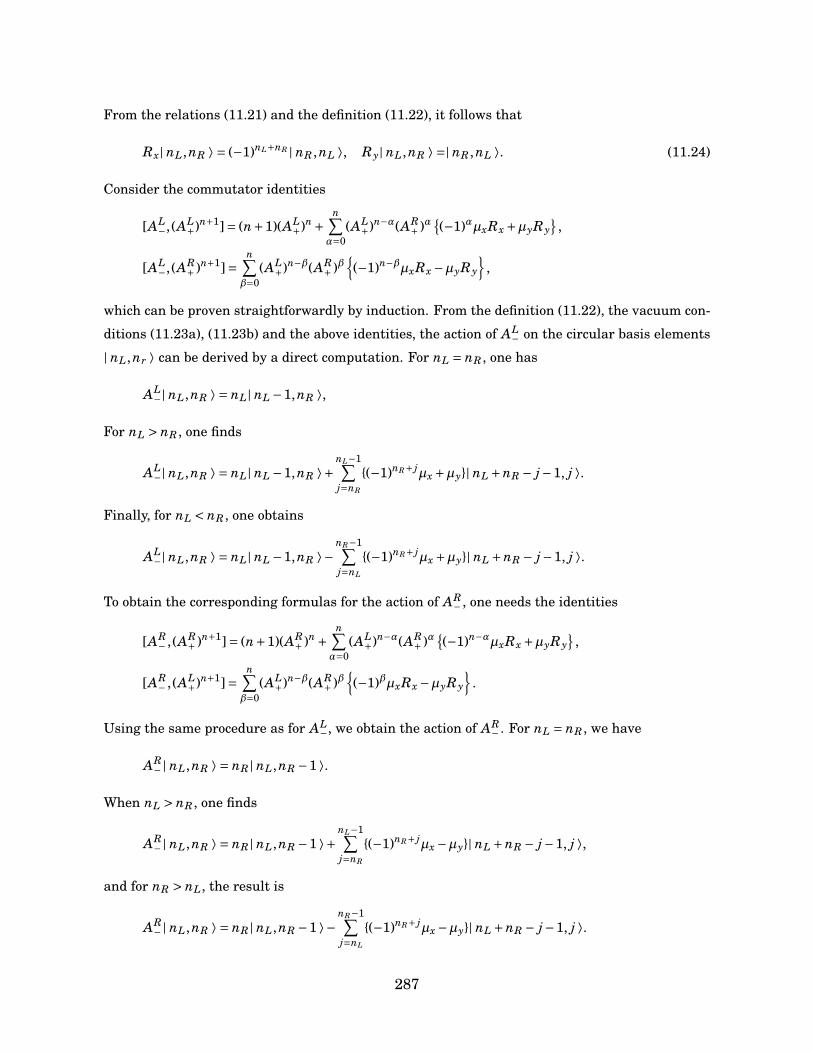
From the relations (11.21) and the definition (11.22), it follows that
Rx| nL,nR ⟩ = (−1)nL+nR | nR ,nL ⟩, Ry| nL,nR ⟩ =| nR ,nL ⟩. (11.24)
Consider the commutator identities
[AL−, (AL
+)n+1]= (n+1)(AL+)n +
n∑α=0
(AL+)n−α(AR
+ )α(−1)αµxRx +µyRy
,
[AL−, (AR
+ )n+1]=n∑
β=0(AL
+)n−β(AR+ )β
(−1)n−βµxRx −µyRy
,
which can be proven straightforwardly by induction. From the definition (11.22), the vacuum con-
ditions (11.23a), (11.23b) and the above identities, the action of AL− on the circular basis elements
| nL,nr ⟩ can be derived by a direct computation. For nL = nR , one has
AL−| nL,nR ⟩ = nL| nL −1,nR ⟩,
For nL > nR , one finds
AL−| nL,nR ⟩ = nL| nL −1,nR ⟩+
nL−1∑j=nR
(−1)nR+ jµx +µy| nL +nR − j−1, j ⟩.
Finally, for nL < nR , one obtains
AL−| nL,nR ⟩ = nL| nL −1,nR ⟩−
nR−1∑j=nL
(−1)nR+ jµx +µy| nL +nR − j−1, j ⟩.
To obtain the corresponding formulas for the action of AR− , one needs the identities
[AR− , (AR
+ )n+1]= (n+1)(AR+ )n +
n∑α=0
(AL+)n−α(AR
+ )α(−1)n−αµxRx +µyRy
,
[AR− , (AL
+)n+1]=n∑
β=0(AL
+)n−β(AR+ )β
(−1)βµxRx −µyRy
.
Using the same procedure as for AL−, we obtain the action of AR− . For nL = nR , we have
AR− | nL,nR ⟩ = nR | nL,nR −1 ⟩.
When nL > nR , one finds
AR− | nL,nR ⟩ = nR | nL,nR −1 ⟩+
nL−1∑j=nR
(−1)nR+ jµx −µy| nL +nR − j−1, j ⟩,
and for nR > nL, the result is
AR− | nL,nR ⟩ = nR | nL,nR −1 ⟩−
nR−1∑j=nL
(−1)nR+ jµx −µy| nL +nR − j−1, j ⟩.
287
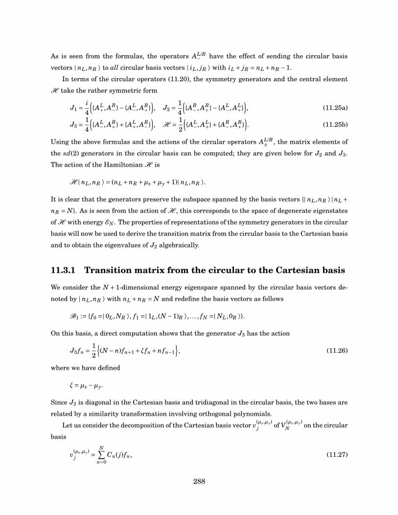
As is seen from the formulas, the operators AL/R− have the effect of sending the circular basis
vectors | nL,nR ⟩ to all circular basis vectors | iL, jR ⟩ with iL + jR = nL +nR −1.
In terms of the circular operators (11.20), the symmetry generators and the central element
H take the rather symmetric form
J1 = i4
(AL
+, AR− − AL
−, AR+
), J2 = 1
4
(AR
− , AR+ − AL
−, AL+
), (11.25a)
J3 = 14
(AL
−, AR+ + AL
+, AR−
), H = 1
2
(AL
−, AL++ AR
− , AR+
). (11.25b)
Using the above formulas and the actions of the circular operators AL/R± , the matrix elements of
the sd(2) generators in the circular basis can be computed; they are given below for J2 and J3.
The action of the Hamiltonian H is
H | nL,nR ⟩ = (nL +nR +µx +µy +1)| nL,nR ⟩.
It is clear that the generators preserve the subspace spanned by the basis vectors | nL,nR ⟩ |nL +nR = N. As is seen from the action of H , this corresponds to the space of degenerate eigenstates
of H with energy EN . The properties of representations of the symmetry generators in the circular
basis will now be used to derive the transition matrix from the circular basis to the Cartesian basis
and to obtain the eigenvalues of J2 algebraically.
11.3.1 Transition matrix from the circular to the Cartesian basis
We consider the N +1-dimensional energy eigenspace spanned by the circular basis vectors de-
noted by | nL,nR ⟩ with nL +nR = N and redefine the basis vectors as follows
B1 := f0 =| 0L, NR ⟩, f1 =| 1L, (N −1)R ⟩, . . . , fN =| NL,0R ⟩.
On this basis, a direct computation shows that the generator J3 has the action
J3 fn = 12
(N −n) fn+1 +ξ fn +nfn−1
, (11.26)
where we have defined
ξ=µx −µy.
Since J3 is diagonal in the Cartesian basis and tridiagonal in the circular basis, the two bases are
related by a similarity transformation involving orthogonal polynomials.
Let us consider the decomposition of the Cartesian basis vector v(µx,µy)j of V (µx,µy)
N on the circular
basis
v(µx,µy)j =
N∑n=0
Cn( j) fn, (11.27)
288

where j ∈ 0, . . . , N. Acting on both sides of (11.27) with J3 and using (11.19c) and (11.26), one
arrives at the following recurrence relation satisfied by the expansion coefficients Cn( j):
(2 j−N)Cn( j)= (n+1)Cn+1( j)+ (N −n+1)Cn−1( j),
with C−1 = 0. Upon factoring out the initial value
Cn( j)= C0( j)Pn( j),
we obtain the recurrence relation
(2 j−N)Pn( j)= (n+1)Pn+1( j)+ (N −n+1)Pn−1( j), (11.28)
where P0( j) = 1. It follows from (11.28) that Pn(x) is a polynomial of degree n in x. Upon substi-
tuting Pn( j)= Pn( j)/n!, we obtain the normalized recurrence relation
( j−N/2)Pn( j)= Pn+1( j)+ 14
n(N −n+1)Pn−1( j).
It is directly seen that the polynomials Pn( j) are the monic Krawtchouk polynomials Kn(x; p, N)
[9] with parameter p = 1/2 and variable x evaluated at x = j. We thus have
Cn( j)= C0( j)Kn( j;1/2, N),
where the constant C0( j) can be chosen to ensure the unitarity of the transition matrix by using
the orthogonality relation of the Krawtchouk polynomials. Despite the differences that the Dunkl
and standard harmonic oscillators exhibit, the relations between the circular and Cartesian bases
are identical in both cases.
11.3.2 Matrix representation of J2 and spectrum
The circular representation space can be used to derive the spectrum of the symmetry operator
J2. To exhibit the structure of J2, we introduce the following notation for the basis vectors:
| nL,nR ⟩ =| `,± ⟩,
where
`= b|nL −nR |/2c, ±= sign(nR −nL),
where bxc is the floor function. We adopt the convention that
sign0=−1
289
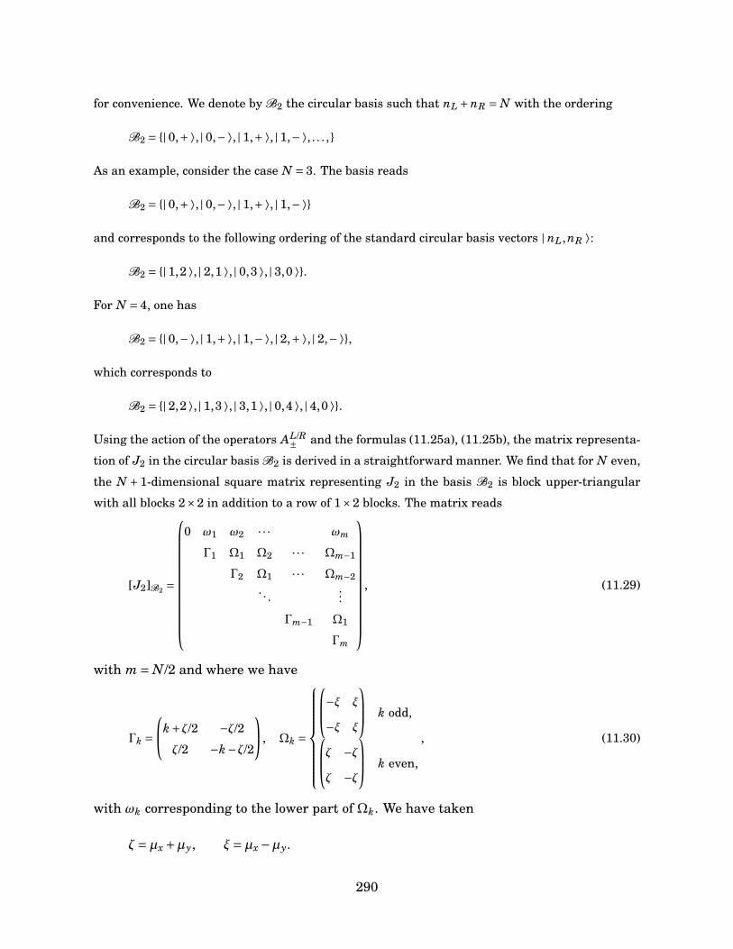
for convenience. We denote by B2 the circular basis such that nL +nR = N with the ordering
B2 = | 0,+ ⟩, | 0,− ⟩, | 1,+ ⟩, | 1,− ⟩, . . . ,
As an example, consider the case N = 3. The basis reads
B2 = | 0,+ ⟩, | 0,− ⟩, | 1,+ ⟩, | 1,− ⟩
and corresponds to the following ordering of the standard circular basis vectors | nL,nR ⟩:
B2 = | 1,2 ⟩, | 2,1 ⟩, | 0,3 ⟩, | 3,0 ⟩.
For N = 4, one has
B2 = | 0,− ⟩, | 1,+ ⟩, | 1,− ⟩, | 2,+ ⟩, | 2,− ⟩,
which corresponds to
B2 = | 2,2 ⟩, | 1,3 ⟩, | 3,1 ⟩, | 0,4 ⟩, | 4,0 ⟩.
Using the action of the operators AL/R± and the formulas (11.25a), (11.25b), the matrix representa-
tion of J2 in the circular basis B2 is derived in a straightforward manner. We find that for N even,
the N +1-dimensional square matrix representing J2 in the basis B2 is block upper-triangular
with all blocks 2×2 in addition to a row of 1×2 blocks. The matrix reads
[J2]B2 =
0 ω1 ω2 · · · ωm
Γ1 Ω1 Ω2 · · · Ωm−1
Γ2 Ω1 · · · Ωm−2. . .
...
Γm−1 Ω1
Γm
, (11.29)
with m = N/2 and where we have
Γk =k+ζ/2 −ζ/2
ζ/2 −k−ζ/2
, Ωk =
−ξ ξ
−ξ ξ
k odd,
ζ −ζζ −ζ
k even,
, (11.30)
with ωk corresponding to the lower part of Ωk. We have taken
ζ=µx +µy, ξ=µx −µy.
290
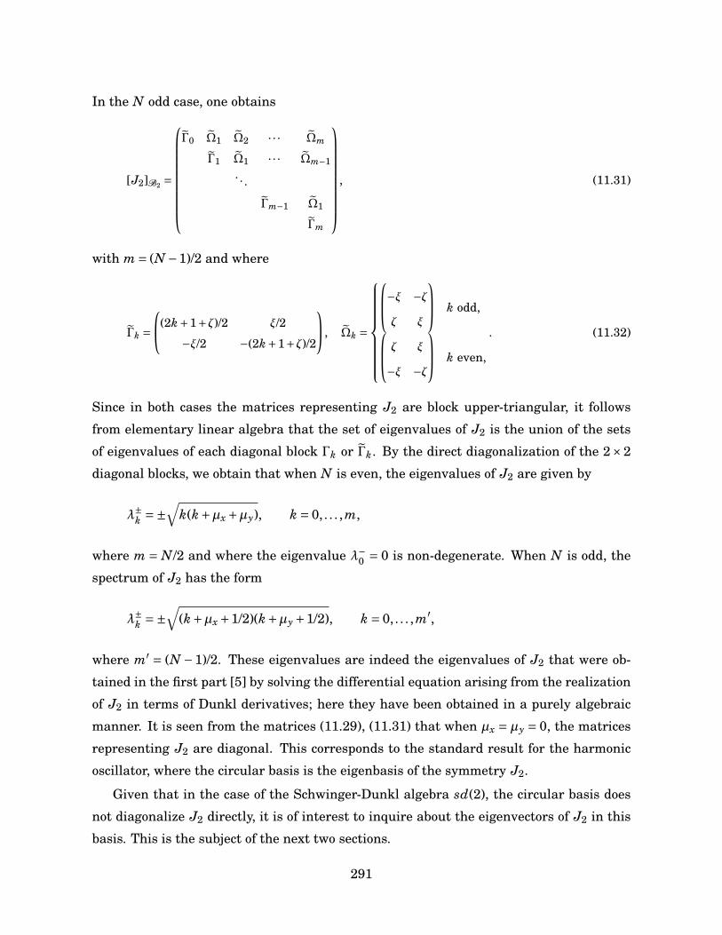
In the N odd case, one obtains
[J2]B2 =
Γ0 Ω1 Ω2 · · · Ωm
Γ1 Ω1 · · · Ωm−1. . .
Γm−1 Ω1
Γm
, (11.31)
with m = (N −1)/2 and where
Γk =(2k+1+ζ)/2 ξ/2
−ξ/2 −(2k+1+ζ)/2
, Ωk =
−ξ −ζζ ξ
k odd,
ζ ξ
−ξ −ζ
k even,
. (11.32)
Since in both cases the matrices representing J2 are block upper-triangular, it follows
from elementary linear algebra that the set of eigenvalues of J2 is the union of the sets
of eigenvalues of each diagonal block Γk or Γk. By the direct diagonalization of the 2×2
diagonal blocks, we obtain that when N is even, the eigenvalues of J2 are given by
λ±k =±
√k(k+µx +µy), k = 0, . . . ,m,
where m = N/2 and where the eigenvalue λ−0 = 0 is non-degenerate. When N is odd, the
spectrum of J2 has the form
λ±k =±
√(k+µx +1/2)(k+µy +1/2), k = 0, . . . ,m′,
where m′ = (N −1)/2. These eigenvalues are indeed the eigenvalues of J2 that were ob-
tained in the first part [5] by solving the differential equation arising from the realization
of J2 in terms of Dunkl derivatives; here they have been obtained in a purely algebraic
manner. It is seen from the matrices (11.29), (11.31) that when µx = µy = 0, the matrices
representing J2 are diagonal. This corresponds to the standard result for the harmonic
oscillator, where the circular basis is the eigenbasis of the symmetry J2.
Given that in the case of the Schwinger-Dunkl algebra sd(2), the circular basis does
not diagonalize J2 directly, it is of interest to inquire about the eigenvectors of J2 in this
basis. This is the subject of the next two sections.
291
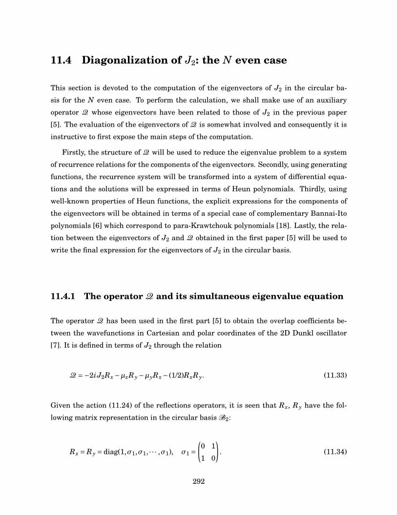
11.4 Diagonalization of J2: the N even case
This section is devoted to the computation of the eigenvectors of J2 in the circular ba-
sis for the N even case. To perform the calculation, we shall make use of an auxiliary
operator Q whose eigenvectors have been related to those of J2 in the previous paper
[5]. The evaluation of the eigenvectors of Q is somewhat involved and consequently it is
instructive to first expose the main steps of the computation.
Firstly, the structure of Q will be used to reduce the eigenvalue problem to a system
of recurrence relations for the components of the eigenvectors. Secondly, using generating
functions, the recurrence system will be transformed into a system of differential equa-
tions and the solutions will be expressed in terms of Heun polynomials. Thirdly, using
well-known properties of Heun functions, the explicit expressions for the components of
the eigenvectors will be obtained in terms of a special case of complementary Bannai-Ito
polynomials [6] which correspond to para-Krawtchouk polynomials [18]. Lastly, the rela-
tion between the eigenvectors of J2 and Q obtained in the first paper [5] will be used to
write the final expression for the eigenvectors of J2 in the circular basis.
11.4.1 The operator Q and its simultaneous eigenvalue equation
The operator Q has been used in the first part [5] to obtain the overlap coefficients be-
tween the wavefunctions in Cartesian and polar coordinates of the 2D Dunkl oscillator
[7]. It is defined in terms of J2 through the relation
Q =−2iJ2Rx −µxRy −µyRx − (1/2)RxRy. (11.33)
Given the action (11.24) of the reflections operators, it is seen that Rx, Ry have the fol-
lowing matrix representation in the circular basis B2:
Rx = Ry = diag(1,σ1,σ1, · · · ,σ1), σ1 =(0 1
1 0
). (11.34)
292
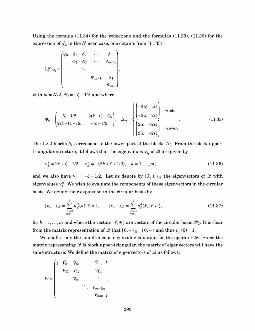
Using the formula (11.34) for the reflections and the formulas (11.29), (11.30) for theexpression of J2 in the N even case, one obtains from (11.33)
[Q]B2 =
φ0 δ1 δ2 · · · δm
Φ1 ∆1 · · · ∆m−1. . .
...
Φm−1 ∆1
Φm,
,
with m = N/2, φ0 =−ζ−1/2 and where
Φk = iζ−1/2 −2ik− (1+ i)ζ
2ik− (1− i)ζ −iζ−1/2
, ∆m =
−2iξ 2iξ
−2iξ 2iξ
modd
2iζ −2iζ
2iζ −2iζ
meven
. (11.35)
The 1×2 blocks δi correspond to the lower part of the blocks ∆i. From the block upper-
triangular structure, it follows that the eigenvalues ν±k of Q are given by
ν+k = 2k+ζ−1/2, ν−k =−(2k+ζ+1/2), k = 1, . . . ,m, (11.36)
and we also have ν−0 = −ζ− 1/2. Let us denote by | k,± ⟩Q the eigenvectors of Q with
eigenvalues ν±k . We wish to evaluate the components of these eigenvectors in the circular
basis. We define their expansion in the circular basis by
| k,+ ⟩Q =k∑
`=0σ=±
uσ` (k)| `,σ ⟩, | k,− ⟩Q =k∑
`=0σ=±
vσ` (k)| `,σ ⟩, (11.37)
for k = 1, . . . ,m and where the vectors | `,± ⟩ are vectors of the circular basis B2. It is clear
from the matrix representation of Q that | 0,− ⟩Q =| 0,− ⟩ and thus v−0 (0)= 1.We shall study the simultaneous eigenvalue equation for the operator Q. Since the
matrix representing Q is block upper-triangular, the matrix of eigenvectors will have thesame structure. We define the matrix of eigenvectors of Q as follows:
W =
1 V01 V02 ··· V0m
V11 V12 ··· V1m
V22...
... Vm−1m
Vmm
,
293
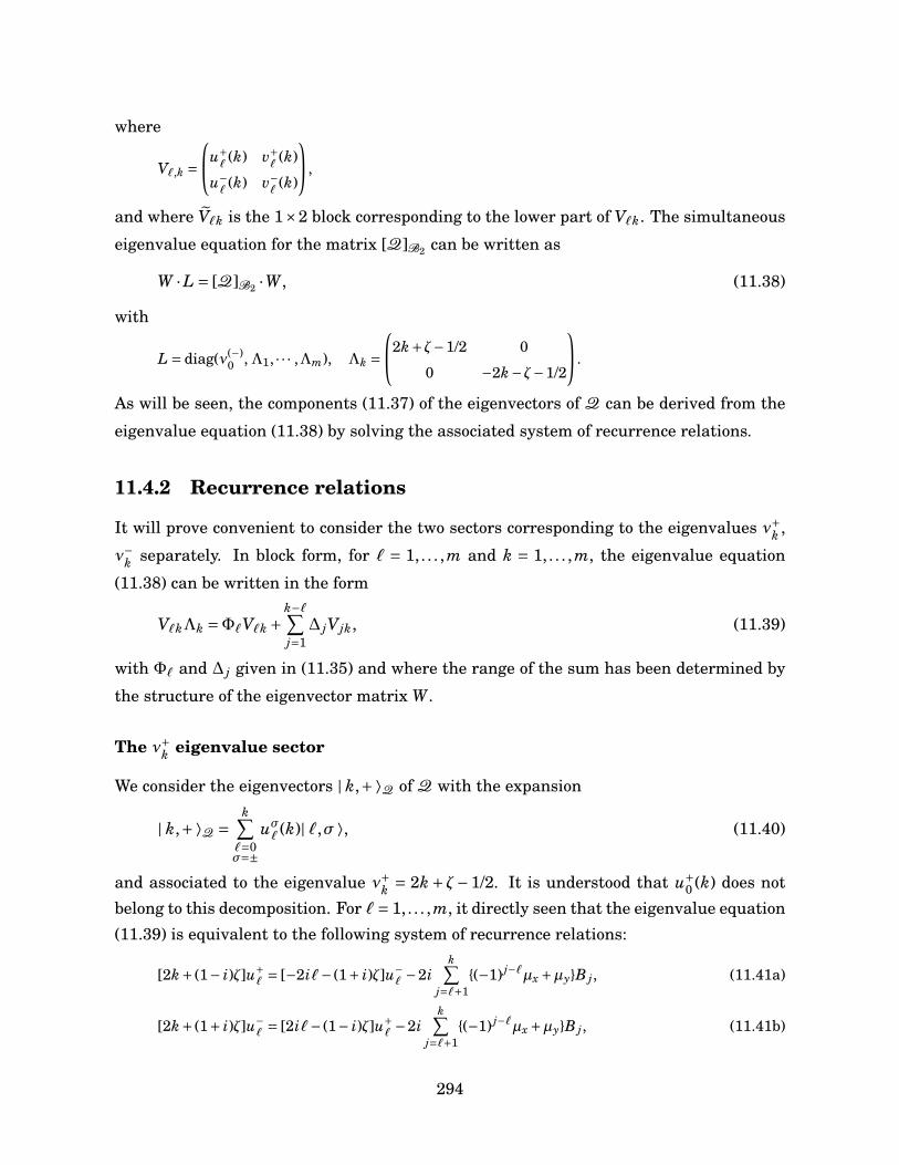
where
V`,k =u+
`(k) v+
`(k)
u−`
(k) v−`
(k)
,
and where V`k is the 1×2 block corresponding to the lower part of V`k. The simultaneous
eigenvalue equation for the matrix [Q]B2 can be written as
W ·L = [Q]B2 ·W , (11.38)
with
L = diag(ν(−)0 ,Λ1, · · · ,Λm), Λk =
2k+ζ−1/2 0
0 −2k−ζ−1/2
.
As will be seen, the components (11.37) of the eigenvectors of Q can be derived from the
eigenvalue equation (11.38) by solving the associated system of recurrence relations.
11.4.2 Recurrence relations
It will prove convenient to consider the two sectors corresponding to the eigenvalues ν+k ,
ν−k separately. In block form, for ` = 1, . . . ,m and k = 1, . . . ,m, the eigenvalue equation
(11.38) can be written in the form
V`kΛk =Φ`V`k +k−∑j=1∆ jVjk, (11.39)
with Φ` and ∆ j given in (11.35) and where the range of the sum has been determined by
the structure of the eigenvector matrix W .
The ν+k eigenvalue sector
We consider the eigenvectors | k,+ ⟩Q of Q with the expansion
| k,+ ⟩Q =k∑
`=0σ=±
uσ` (k)| `,σ ⟩, (11.40)
and associated to the eigenvalue ν+k = 2k+ ζ−1/2. It is understood that u+0 (k) does not
belong to this decomposition. For `= 1, . . . ,m, it directly seen that the eigenvalue equation(11.39) is equivalent to the following system of recurrence relations:
[2k+ (1− i)ζ]u+` = [−2i`− (1+ i)ζ]u−
` −2ik∑
j=`+1(−1) j−`µx +µyB j, (11.41a)
[2k+ (1+ i)ζ]u−` = [2i`− (1− i)ζ]u+
` −2ik∑
j=`+1(−1) j−`µx +µyB j, (11.41b)
294
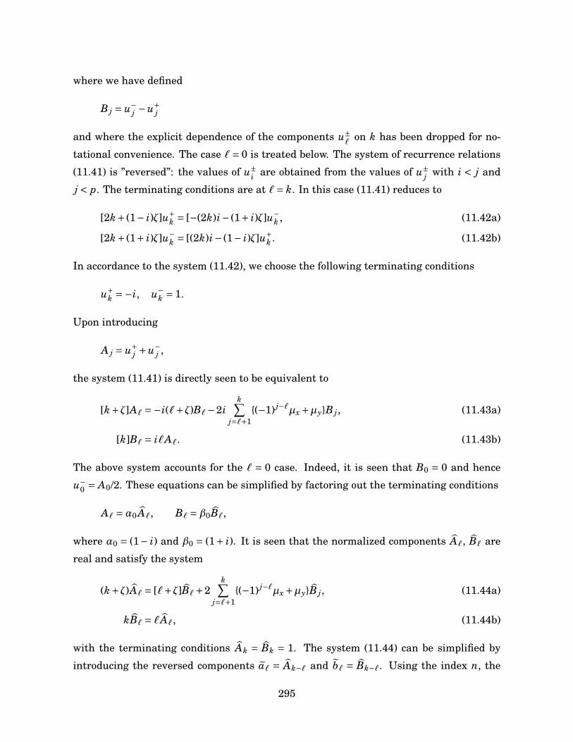
where we have defined
B j = u−j −u+
j
and where the explicit dependence of the components u±`
on k has been dropped for no-
tational convenience. The case `= 0 is treated below. The system of recurrence relations
(11.41) is ”reversed”: the values of u±i are obtained from the values of u±
j with i < j and
j < p. The terminating conditions are at `= k. In this case (11.41) reduces to
[2k+ (1− i)ζ]u+k = [−(2k)i− (1+ i)ζ]u−
k , (11.42a)
[2k+ (1+ i)ζ]u−k = [(2k)i− (1− i)ζ]u+
k . (11.42b)
In accordance to the system (11.42), we choose the following terminating conditions
u+k =−i, u−
k = 1.
Upon introducing
A j = u+j +u−
j ,
the system (11.41) is directly seen to be equivalent to
[k+ζ]A` =−i(`+ζ)B`−2ik∑
j=`+1(−1) j−`µx +µyB j, (11.43a)
[k]B` = i`A`. (11.43b)
The above system accounts for the ` = 0 case. Indeed, it is seen that B0 = 0 and hence
u−0 = A0/2. These equations can be simplified by factoring out the terminating conditions
A` =α0 A`, B` =β0B`,
where α0 = (1− i) and β0 = (1+ i). It is seen that the normalized components A`, B` are
real and satisfy the system
(k+ζ)A` = [`+ζ]B`+2k∑
j=`+1(−1) j−`µx +µyB j, (11.44a)
kB` = `A`, (11.44b)
with the terminating conditions Ak = Bk = 1. The system (11.44) can be simplified by
introducing the reversed components a` = Ak−` and b` = Bk−`. Using the index n, the
295
system takes the usual form
(k+ζ)an = (k−n+ζ)bn +2n−1∑α=0
(−1)n+αµx +µybα (11.45a)
k bn = (k−n)an, (11.45b)
with the initial conditions a0 = b0 = 1. Hence the components u±`
(k) of the eigenvector| k,± ⟩Q of the operator Q have the expression
u−` (k)= α0ak−`+β0bk−`
2, u+
` (k)= α0ak−`−β0bk−`2
, (11.46)
where an and bn are the unique solutions to the system (11.45).
The ν−k eigenvalue sector
We consider the eigenvectors | k,− ⟩Q corresponding to the eigenvalue ν−k of Q with the
circular basis expansion
| k,− ⟩Q =k∑
`=0σ=±
vσ` (k)| `,σ ⟩,
and associated eigenvalue ν−k = −2k− ζ−1/2. An analysis similar to the preceding oneshows that the components v±
`(k) differ from the components u±
`(k) only by their termi-
nating conditions. Again choosing v−k (k)= 1, we find
v+k (k)= (1+ i)k+ζ(1− i)k−ζ , v−k (k)= 1.
This yields
v−` (k)= γ0ak−`+ε0bk−`2
, v+` (k)= γ0ak−`+ε0bk−`2
, (11.47)
where
γ0 = 2i(k+ζ)(1+ i)k+ iζ
, ε0 = 2k(1+ i)k+ iζ
,
and where v−0 = γ0ak.
11.4.3 Generating function and Heun polynomials
We have seen that the evaluation of the components of the eigenvectors of Q in the cir-
cular basis depends on the solution of the recurrence system (11.45). As it turns out, an
explicit solution for an(k) and bn(k) can be obtained using generating functions.
296
We introduce the ordinary generating functions
A(z)= ∑n>0
anzn, B(z)= ∑n>0
bnzn.
We shall make use of the elementary identities
z∂z A(z)= ∑n>0
nanzn, (1− z)−1 A(z)= ∑n>0
( ∑06k6n
ak
)zn, (11.48a)
(1+ z)−1 A(z)= ∑n>0
( ∑06k6n
(−1)k+nak
)zn. (11.48b)
Using the above identities, it is easily seen that the system of recurrence relations (11.45)for the quantities an, bn is equivalent to the following system of differential equations forthe generating functions A(z), B(z):
(k+ζ)A(z)= (k−ζ− z∂z)B(z)+ 2µx
1+ zB(z)+ 2µy
1− zB(z), (11.49a)
kB(z)= (k− z∂z)A(z). (11.49b)
By direct substitution, we find that the generating function A(z) satisfies the second-orderdifferential equation
A′′(z)+(
1−2k−ζz
+ 2µy
z−1+ 2µx
1+ z
)A′(z)+
( −2kζz+2kξz(z−1)(z+1)
)A(z)= 0. (11.50)
This corresponds to Heun’s differential equation [3, 13]. The general form of the Heundifferential equation is
w′′(z)+(γ
z+ δ
z−1+ ε
z−a
)w′(z)+ αβz− q
z(z−1)(z−a)w(z)= 0, (11.51)
with α+β+1= γ+δ+ε. Comparing (11.51) with (11.50), we thus write
A(z)= H`(a, q;α,β,γ,δ, z) (11.52)
with the parameters
a =−1, q = 2k(µy −µx), α=−2k, (11.53a)
β=µx +µy, γ= 1−2k−µx −µy, δ= 2µy. (11.53b)
The function H`(a, q;α,β,γ,δ) denotes the solution to (11.51) that corresponds to the ex-
ponent 0 at z = 0 and assumes the value 1 at that point. This is obviously the case of A(z).
It will be seen that A(z) is in fact a polynomial of degree 2k, and hence that the Heun
function (11.52) is in fact a Heun polynomial. Given the system (11.49), we also have
B(z)= k−1(k− z∂z)A(z).
297
11.4.4 Expansion of Heun polynomials in the
complementary Bannai-Ito polynomials
The well-studied properties of Heun functions can be used to obtain a closed form formula
for the coefficients an and hence for bn. In what follows, it will be shown that the Heun
polynomial in (11.52) can be expanded in terms of a special case of the complementary
Bannai-Ito polynomials corresponding to the para-Krawtchouk polynomials.
Consider the solution H`(a, q;α,β,γ,δ) to the equation (11.51) and its Maclaurin ex-
pansion
H`(a, q;α,β,γ,δ)=∞∑
n=0cnzn,
where c−1 = 0, c0 = 1. The coefficients cn obey the three-term recurrence relation [3, 13]
Rncn+1 − (Qn + q)cn +Pncn−1 = 0,
where
Rn = a(n+1)(n+γ), Qn = n[(n−1+γ)(1+a)+aδ+ε], (11.54a)
Pn = (n−1+α)(n−1+β). (11.54b)
The identification of A(z) as a Heun function enables one to reduce the evaluation of
an to the solution of a three-term recurrence relation. It is seen that with the choice of
paramaters (11.53), the expansion coefficients cn of the Heun function A(z) truncate at
degree k = 2n. Hence A(z) is a polynomial of degree 2k in z. For convenience, we use
the symbol Pn = an in the computations to follow. Using the parameters (11.53) in the
recurrence coefficients (11.54) for the expansion coefficients in
A(z)= ∑n>0
Pnzn,
we can obtain the recurrence relation for Pn. Upon setting N = 2k and dividing by (N−2n)
we find that Pn(ξ) is a symmetric polynomial of degree n in the variable ξ obeying the
recurrence relation
σn+1Pn+1(ξ)−κnPn−1(ξ)= ξPn(ξ),
with P−1 = 0, P1 = 1 and where
σn = n(N +ζ−n)(2n−N −2)
, κn = (N +1−n)(n+ζ−1)(2n−N)
.
298
As k takes integer values, it is seen that when k = n, a singularity appears in the recur-
rence relation. Notwithstanding this, we proceed with the computation; the effect of the
pole in k = n on the results is treated below.
Introducing the monic polynomials Pn(ξ)= Pn(ξ)σ1···σn
, the recurrence relation becomes
Pn+1(ξ)+unPn−1(ξ)= ξPn(ξ), (11.55)
where
un =−n(N +1−n)(N −n+ζ)(n+ζ−1)(N −2n)(N −2n+2)
.
The monic polynomials Pn(ξ) can be identified with the complementary Bannai-Ito poly-
nomials (CBI).
The monic CBI polynomials [6, 16], denoted In(x;ρ1,ρ2, r1, r2), obey the recurrence
relation
In+1(x)+ (−1)nρ2In(x)+τnIn−1(x)= xIn(x), (11.56)
where
τ2n =−n(n+ρ1 − r1 +1/2)(n+ρ1 − r2 +1/2)(n− r1 − r2)(2n+ g)(2n+ g+1)
, (11.57a)
τ2n+1 =− (n+ g+1)(n+ρ1 +ρ2 +1)(n+ρ2 − r1 +1/2)(n+ρ2 − r2 +1/2)(2n+ g+1)(2n+ g+2)
(11.57b)
and with g = ρ1 +ρ2 − r1 − r2. They have the hypergeometric representation
I2n(x)= Rn(x), I2n+1(x)= (x−ρ2)Qn(x),
where
Rn(x)= ηn 4F3
[ −n,n+ g+1,ρ2 + x,ρ2 − xρ1 +ρ2 +1,ρ2 − r1 +1/2,ρ2 − r2 +1/2
;1], (11.58)
Qn(x)= ιn 4F3
[ −n,n+ g+2,ρ2 + x+1,ρ2 − x+1ρ1 +ρ2 +2,ρ2 − r1 +3/2,ρ2 − r2 +3/2
;1], (11.59)
with
ηn = (ρ1 +ρ2 +1)n(ρ2 − r1 +1/2)n(ρ2 − r2 +1/2)(n+ g+1)n
,
ιn = (ρ1 +ρ2 +2)n(ρ2 − r1 +3/2)n(ρ2 − r2 +3/2)(n+ g+2)n
,
and where (a)n = (a)(a+1) · · · (a+n−1) is the Pochhammer symbol.
299
Comparing the recurrence formulas (11.55) with (11.56) and (11.57), it is seen that the
polynomials Pn(ξ) are monic CBI polynomials
Pn(ξ)= In(ξ/2;ρ1,ρ2, r1, r2
), (11.60)
with
ρ1 = ζ−22
, ρ2 = 0, r1 = 2k+ζ2
, r2 = 0. (11.61)
The parametrization (11.61) is a special case of CBI polynomials. This case corresponds
to the para-Krawtchouk polynomials constructed in [18] in the context of perfect state
transfer in spin chains.
Since there is a singularity in the recurrence coefficients for the polynomials Pn(ξ),
the correspondence between the polynomials Pn(ξ) and the CBI polynomials outlined
above is valid only for n = 0, . . . ,k and hence the Heun polynomial A(z) generates only
the first k para-Krawtchouk polynomials. As is easily seen by induction, the recurrence
relation (11.55) generates center-symmetric polynomials Pn. Hence for n > k, we have
Pn(ξ)=P2k−n(ξ). Putting the preceding results together, we write
an = (−1)n4n
n!(k+1−n)n
(2k+ζ−n)nIn(ξ/2;ρ1,ρ2, r1, r2) (11.62)
for n6 k and
an = a2k−n, n = k+1, . . . ,2k
for n = k+1 · · · ,2k.
The hypergeometric expression of the CBI polynomials (11.58) provides an explicit
formula for the coefficients an and the coefficients bn are easily evaluated from the re-
currence system (11.45). Combining those results with the formulas (11.46) and (11.47)
yields the expansion coefficients of the eigenvectors of the operator Q in the circular ba-
sis. Note that these expansion coefficients only involve a j, b j with j = 0, . . . ,k and hence
only (11.62) is needed.
11.4.5 Eigenvectors of J2
To obtain the expansion coefficients of the eigenvectors of J2 in the circular basis, it is
necessary to relate the eigenvectors of J2 to those of Q. This relation has been obtained
300
in the previous paper [5]. In the present notation, we have
| k,+ ⟩Q = 1p2
(| k,+ ⟩J2 −ωk| k,− ⟩J2
),
| k,− ⟩Q = 1p2
(| k,+ ⟩J2 +ωk| k,− ⟩J2
)where | k,± ⟩J2 are the eigenvectors of J2 corresponding to the eigenvalues
λ± =√
k(k+ζ),
and where the coefficient ωk is
ωk =ζ−2i
√k(k+ζ)
2k+ζ .
The inverse relation, which allows to express the eigenvectors of J2 in terms of the known
eigenvectors of Q reads
| k,+ ⟩J2 =1p2
(| k,+ ⟩Q+| k,− ⟩Q) ,
| k,− ⟩J2 =−1
ωkp
2(| k,+ ⟩Q−| k,− ⟩Q) .
11.4.6 The fully isotropic case
We now consider the case µx = µy = µ. This corresponds to a fully isotropic 2D Dunkl
oscillator, where two "identical" parabosonic oscillators are combined. Returning to the
system of differential equations (11.49) for the generating functions, one has
(k+2µ)A(z)= (k−2µ− z∂z)B(z)+ 4µ1− z2 B(z),
kB(z)= (k− z∂z)A(z).
Solving for A(z), we find
z(z2 −1)A′′(z)+ (z2(2µ+1−2k)+2µ+2k−1
)A′(z)−4kµzA(z)= 0.
The solution corresponding to the initial value a0 = 1 is given by
A(z)= 2F1
[ −k,µ1−k−µ ; z2
],
and we also have
B(z)= A(z)− 2kµz2
k+µ−1 2F1
[1−k,1+µ2−k−µ ; z2
].
301
Hence in the isotropic case, the generating functions are simply the Jacobi polynomials.
It follows from the hypergeometric generating function that
a2n = (−k)n(µ)n
(1−k−µ)nn!, a2n+1 = 0,
and
b2n =(
k−2nk
)(−k)n(µ)n
(1−k−µ)nn!, b2n+1 = 0.
Thus it is seen that the in the fully isotropic case µx =µy =µ, the formulas for the expan-
sion coefficients of the eigenvectors of Q simplify substantially.
11.5 Diagonalization of J2: the N odd case
In this section, we obtain the expression for the eigenvectors of J2 in the circular basis
when N = nL +nR is an odd integer. In spirit, the computation is similar to the N even
case presented in the previous section. We proceed along the same lines.
11.5.1 The operator Q and its simultaneous eigenvalue equation
The operator Q is defined by
Q =−2iJ2Rx −µxRy −µyRx − (1/2)RxRy.
Given the action (11.24) of the reflections operators, it is seen that they have the following
matrix representation in the circular basis B2 :
Ry =−Rx = diag(σ1, . . . ,σ1), σ1 =(0 1
1 0
).
Using the matrix representation of J2 in the circular basis B2 given in (11.31), one finds
[Q]B2 =
Φ0 ∆1 ∆2 · · · ∆m
Φ1 ∆1 · · · ∆m−1. . .
Φm−1 ∆1
Φm
,
302
with m = (N −1)/2 and where
Φk = 1/2+ iξ i(2k+ζ+1)−ξ−i(2k+ζ+1)−ξ 1/2− iξ
, ∆m =
−2iζ −2iξ
2iξ 2iζ
m odd
2iξ 2iζ
−2iζ −2iξ
m even
. (11.63)
From the block upper-triangular structure, it follows that the eigenvalues ν±k of Q are
ν+k = 2k+ζ+3/2, ν−k =−(2k+ζ+1/2),
for k = 0, . . . ,m. Although a different labeling has been used, it is directly checked that the
eigenvalues of Q are the same for the N even and N odd case, except for the additional
one. We denote the eigenvectors of Q corresponding to the eigenvalues ν±k by | k,± ⟩Q and
define their expansion in the circular basis by
| k,+ ⟩Q =k∑
`=0σ=±
uσ` (k)| `,σ ⟩, | k,− ⟩Q =k∑
`=0σ=±
vσ` (k)| `,σ ⟩,
for k = 0, . . . ,m and where the vectors | `,± ⟩ are the vectors of the circular basis B2.We shall once again study the simultaneous eigenvalue equation for the operator Q.
We define the matrix of eigenvectors
W =
V00 V01 · · · V0m
V11 · · · V1m. . .
Vmm
,
where
V`k =v+
`(k) u+
`(k)
v−`
(k) u−`
(k)
.
The simultaneous eigenvalue equation for the matrix [Q]B2 reads
W ·L = [Q]B2W , (11.64)
with
L = diag(Λ0, · · · ,Λm), Λk =ν−k 0
0 ν+k
. (11.65)
As in section 4, the simultaneous equation (11.64) will be shown to be equivalent to a
system of recurrence relation for the components u`(k)±, v±`
(k) of the eigenvectors of Q in
the circular basis.
303
11.5.2 Recurrence relations
We now construct the recurrence systems for the component of the eigenvectors of the
operator Q. For k = 0, . . . ,m and `= 0, . . . ,m, the simultaneous equation (11.64) takes the
form
V`kΛk = Φ`V`k +k−∑j=1∆ jVjk. (11.66)
The ν−k eigenvalue sector
Let us begin by considering the eigenvectors | k,− ⟩Q of Q corresponding to the eigenvalue
ν−k and their expansion in the circular basis
| k,− ⟩Q =k∑
`=0σ=±
vσ` (k)| `,σ ⟩.
It is directly seen from (11.66),(11.63) and (11.65) that we have
[2k+1+ζ+ iξ]v+` = [ξ− i(2`+ζ+1)]v−` −2iµx
k∑j=`+1
(−1) j−`A j −2iµy
k∑j=`+1
B j, (11.67a)
[2k+1+ζ− iξ]v−` = [ξ+ i(2`+ζ+1)]v+` +2iµx
k∑j=`+1
(−1) j−`A j −2iµy
k∑j=`+1
B j, (11.67b)
where we have defined A j = v+j +v−j and B j = v−j −v+j and where the explicit dependence on
k of the components v±`
(k) has been dropped for notational convenience. The recurrence
system (11.67) is ”reversed”. The terminating conditions are at `= k. In this case, (11.67)
becomes
[2k+1+ζ+ iξ]v+k = [ξ− i(2k+ζ+1)]v−k ,
[2k+1+ζ− iξ]v−k = [ξ+ i(2k+ζ+1)]v+k .
Choosing v−k = 1, we obtain the terminating conditions
v+k =−i, v−k = 1.
Upon taking
A` =α0 A`, B` =β0B`,
304
where α0 = (1− i) and β0 = (1+ i), it is easily seen that A` and B` are real and that thesystem (11.67) is equivalent to
[k+µy +1/2]A` = (`+µy +1/2)B`+2µy
k∑j=`+1
B j,
[k+µx +1/2]B` = (`+µx +1/2)A`+2µx
k∑j=`+1
(−1) j−` A j,
with the terminating conditions Ak = 1 and Bk = 1. Introducing the reversed components
an = Ak−n, bn = Bk−n, we obtain the system
[k+µy +1/2]an = [k−n+µy +1/2]bn +2µy
n−1∑j=0
b j, (11.68a)
[k+µx +1/2]bn = [k−n+µx +1/2]an +2µx(−1)nn−1∑j=0
(−1) j a j, (11.68b)
with the initial conditions a0 = 1 and b0 = 1. Taking into account all the preceding trans-formations, we have
v−` (k)= α0ak−`+β0bk−`2
, v+` (k)= α0ak−`−β0bk−`2
, (11.69)
where a`, b` are the unique solutions to the recurrence system (11.68).
The ν+k eigenvalue sector
Let us now consider the eigenvectors | k,+ ⟩Q corresponding to the eigenvalue ν+k with
expansion
| k,+ ⟩Q =k∑
`=0σ=±
uσ` (k)| `,σ ⟩,
in the circular basis. Proceeding along the same lines as in the previous computation, we
find that the terminating condition are of the form
v+k = i(2k+1+ζ+ iξ)2k+1+ζ− iξ
, v−k = 1,
and that the components are given by
u−` (k)= γ0ak−`+ε0bk−`
2, u+
` (k)= γ0ak−`−ε0bk−`2
, (11.70)
where
γ0 =(1+ i)(2k+1+2µy)
2k+1+ζ− iξ, ε0 = (1− i)(2k+1+2µx)
2k+1+ζ− iξ.
305
11.5.3 Generating functions and Heun polynomials
As is seen from the formulas (11.69) and (11.70), the main part of the components of the
eigenvectors of Q in the circular basis is given by the solutions to the recurrence system
(11.68). As in section 4 for the N even case, we bring the ordinary generating functions
A(z)=∑n
anzn, B(z)=∑n
bnzn.
Upon using the identities (11.48), we obtain from (11.68) the associated differential sys-tem
(k+µy +1/2)A(z)= (k−µy +1/2− z∂z)B(z)+ 2µy
1− zB(z), (11.71a)
(k+µx +1/2)B(z)= (k−µx +1/2− z∂z)A(z)+ 2µx
1+ zA(z). (11.71b)
By direct substitution, we find that the generating functions are expressed in terms of the
Heun functions
A(z)= (1+ z)H`(a, qA;αA,βA,γA,δA, z), (11.72a)
B(z)= (1− z)H`(a, qB;αB,βB,γB,δB,−z), (11.72b)
where
a =−1, qA = 2k(µy −µx −1), αA =−2k, (11.73a)
βA =µx +µy +1, γA =−2k−µx −µy, δA = 2µy. (11.73b)
and where the parameters qB, · · ·δB are obtained from (11.73) by the transformation µx ↔µy. The form of the parameters involved in the Heun functions show that once again one
has a truncation at degree 2k+1 and hence the Heun functions appearing in (11.72) are in
fact Heun polynomials. The generating functions A(z) and B(z) are polynomials of degree
2k+1.
11.5.4 Expansion of Heun polynomials in
complementary Bannai-Ito polynomials
The expansion of the Heun polynomials can be obtained using the associated three-term
recurrence relation. Since the expansion coefficients of B(z) and A(z) are related by the
simple relation z ↔−z and µx ↔µy, we shall focus on the expansion of A(z).
306
We examine the expansion of the Heun polynomial appearing in (11.72a)
H`(a, qA,αA,βA,γA,δA, z)=∑r
P r zr, (11.74)
where the parameters are given in (11.73). Using the recurrence coefficients given in
(11.54), one finds that the expansion coefficients Pn are polynomials of degree r in ξ =µx −µy that obey the recurrence relation
σr+1P r+1(ξ)+κrP r−1(ξ)= (1+ξ)P r(ξ), (11.75)
with P−1 = 0, P0 = 1 and where
σr+1 = (r+1)(N +ζ− r)2r−N
, κr = (N +1− r)(r+ζ)2r−N
,
where we have taken N = 2k. Introducing the monic polynomials P r(ξ)= P r(ξ)σ1···σr
, we obtain
P r+1(ξ)+urP r−1(ξ)= (1+ξ)P r(ξ) (11.76)
where
ur =− r(N +1− r)(N +ζ− r−1)(r+ζ)(N −2r)(N −2r+2)
.
Upon comparing (11.76) with the recurrence coefficients for the CBI polynomials given in
(11.57), it is directly seen that the polynomials defined by the recurrence (11.76) corre-
spond to CBI polynomials with the parametrization
ρ1 = ζ−12
, r1 = 2k+ζ+12
, ρ = 0, r2 = 0. (11.77)
Hence, when r 6 k, we have
P r(ξ)= (−1)r4r
r!(k+1− r)r
(2k+ζ+1− r)rIr((1+ξ)/2;ρ1,ρ2, r1, r2), r 6 k, (11.78)
where ρ1, ρ2, r1 and r2 are given by (11.77) and In(x;ρ1,ρ2, r1, r2) are the complementary
Bannai-Ito polynomials. As can be seen by the recurrence relation (11.75), the expansion
coefficients of the Heun function (11.74) truncate at order 2k+1 and are center-symmetric.
Hence, for r > k, we have
P r(ξ)=P2k+1−r(ξ), r > k. (11.79)
307
Taking into account the relation between A(z) and B(z), the expansion coefficients of the
Heun function appearing in (11.72b), denoted by Tn(ξ), are easily seen to be
Tr(ξ)= 4r
r!(k+1− r)r
(2k+ζ+ r−1)rIr((1−ξ)/2;ρ1,ρ2, r1, r2), r 6 2k, (11.80)
Tr(ξ)=T2k+1−r(ξ), r > 2k. (11.81)
Collecting all the previous results, we write
an =Pn(ξ)+Pn−1(ξ), (11.82a)
bn =Tn(ξ)+Tn−1(ξ), (11.82b)
where P−1 = 0, T−1 = 0 and Pn(ξ), Tn(ξ) are given by (11.78), (11.79), (11.80) and (11.81).
11.5.5 Eigenvectors of J2
To obtain the expansion of the eigenvectors of J2 in the circular basis, one must relate the
eigenvectors of the operator Q to the eigenvectors of J2. This relation has been obtained
in the previous paper [5]. We have
| k,± ⟩Q = 1p2
(| k,+ ⟩J2 ∓υk| k,− ⟩J2
)where | k,± ⟩J2 are the eigenvectors of J2 corresponding to the eigenvalues
λ±k =±
√(k+µx +1/2)(k+µy +1/2), k = 0, . . . ,m,
and where
vk =[ξ+2i
√(k+µx +1/2)(k+µy +1/2)
2k+ζ+1
].
The inverse relation reads
| k,+ ⟩J2 =1p2
(| k,+ ⟩Q+| k,− ⟩Q) , (11.83a)
| k,− ⟩J2 =−1
vkp
2(| k,+ ⟩Q−| k,− ⟩Q) (11.83b)
Using the relations (11.83), the results (11.82), (11.70) and (11.69), one has an explicit
expression for the expansion of the eigenvectors of J2 in the circular basis for the case N
odd.
308
11.5.6 The fully isotropic case : −1 Jacobi polynomials
We consider again the case µx = µy = µ which corresponds to the fully isotropic Dunkl os-
cillator, where two independent identical parabosonic oscillators are combined. We return
to the system of differential equations for the generating functions of the components of
the eigenvectors of Q given in (11.71). When µx =µy =µ, one has
(k+µ+1/2)A(z)= (k−µ+1/2− z∂z)B(z)+ 2µ1− z
B(z),
(k+µ+1/2)B(z)= (k−µ+1/2− z∂z)A(z)+ 2µ1+ z
A(z).
It is easily seen from the above formulas that A(z)= B(−z). Hence the generating function
A(z) satisfies the differential equation
(k+µ+1/2)A(z)= (k−µ+1/2− z∂z)A(−z)+ 2µ1− z
A(−z),
which may be cast in the form of an eigenvalue equation
LA(z)= 4µA(z),
where
L = 2(1− z)∂zR+[(−2k−1+2µ)+ 2k+1+2µ
z
](I−R),
where R f (z) = f (−z). It is recognized that the operator L is a special case of the defining
operator of the little −1 Jacobi polynomials [17].
The little −1 Jacobi polynomials, denoted by P−1n (x), obey the eigenvalue equation
ΩPn(x)=λnPn(x), λn =
−2n n even
2(α+β+n+1) n odd,
where
Ω= 2(1− x)∂xR+ (α+β+1−α/x)(I−R).
Comparing the operatorsΩ and L, it is seen that the generating function A(z) corresponds
to a −1 Jacobi polynomial of degree n = 2k+1 with parameters
α=−2k−2µ−1, β= 4µ−1.
309
Using this identification and the explicit formula for the little −1 Jacobi polynomials de-
rived in [17], we obtain
A(z)= 2F1
[ −k,µ−µ−k
; z2]+ µz
k+µ 2F1
[ −k,µ+1−k−µ+1
; z2].
This directly yields the following result for the recurrence coefficients an:
a2n = (−k)n(µ)n
n!(−µ−k)n, a2n+1 = µ
k+µ(−k)n(µ+1)n
n!(−µ−k+1)n.
Using the symmetry B(z)= A(−z), we also obtain
b2n = (−k)n(µ)n
n!(−µ−k)n, b2n+1 = −µ
k+µ(−k)n(µ+1)n
n!(−µ−k+1)n.
Once again, the components of the eigenvectors of Q drastically simplify in the isotropic
case µx =µy =µ. Moreover, the preceding computations entail a relation between a special
case of Heun polynomials and the little −1 Jacobi polynomials.
11.6 Representations of sd(2) in the J2 eigenbasis
We now investigate the representation space in which the operator J2 is diagonal. The
matrix elements of the generators of the Schwinger-Dunkl algebra will be derived using
the defining relations of sd(2), which read
J1,Rxi = 0, J2,Rxi = 0, [J3,Rxi ]= 0,
[J2, J3]= iJ1, [J3, J1]= iJ2,
[J1, J2]= i[J3 + J3(µxRx +µyRy)−H (µxRx −µyRy)/2],
where R2x = R2
y = I. It will prove convenient to treat the even and odd dimensional repre-
sentations separately.
11.6.1 The N odd case
We first consider the case where N is odd. The representation space C is spanned in this
case by the basis vectors | k,± ⟩ with k ∈ 0, . . . ,m on which the generator J2 acts in a
diagonal fashion
J2| k,± ⟩=λ±k | k,± ⟩, k = 0, . . . ,m,
310
where m = (N −1)/2 and where the eigenvalues of J2, derived in section 3, are given by
λ±k =±
√(k+µx +1/2)(k+µy +1/2), k = 0, . . . ,m.
Since Rx, Ry anti-commute with J2 and given that RxRy is central in the algebra sd(2),
we can take
Rx| k,± ⟩= ε| k,∓ ⟩, Ry| k,± ⟩=| k,∓ ⟩,
where ε = ±1. Here we choose ε = −1, which corresponds to the representation encoun-
tered in the model. In the basis | 0,+ ⟩, | 0,− ⟩, · · · , | m,+ ⟩, | m,− ⟩, the matrices represent-
ing the involutions Rx, Ry have the form
Ry =−Rx = diag(σ1, . . . ,σ1), σ1 =(0 1
1 0
),
which is identical to their action in the circular basis. The Hamiltonian H has the action
H | k,± ⟩= (N +µx +µy +1)| k,± ⟩.
The action of the operator J3 on this representation space can be derived by imposing the
commutation relation (11.6) using (11.6) to define J1. The action of J3 on the basis | k,± ⟩is taken to be
J3| k,+ ⟩=m∑
j=0σ=±
Mσjk| j,σ ⟩, J3| k,− ⟩=
m∑j=0σ=±
Nσjk| j,σ ⟩.
With these definitions, it is easily seen that the commutation relation (11.6) is equivalentto the following system of relations
[(λ+k )2 −2(λ+
j λ+k )+ (λ+
j )2 −1]M+jk = (µy −µx)N+
jk, (11.84a)
[(λ+k )2 −2(λ−
j λ+k )+ (λ−
j )2 −1]M−jk = (µy −µx)N−
jk +δ jkζ(N +1+ζ)
2, (11.84b)
[(λ−k )2 −2(λ+
j λ−k )+ (λ+
j )2 −1]N+jk = (µy −µx)M+
jk +δ jkζ(N +1+ζ)
2, (11.84c)
[(λ−k )2 −2(λ−
j λ−k )+ (λ−
j )2 −1]N−jk = (µy −µx)M−
jk, (11.84d)
where the relations (11.84a),(11.84b) were obtained by acting on | k,+ ⟩ and the relations(11.84c),(11.84d) by acting on | k,− ⟩. It follows directly from the solution of the system(11.84) that J3 acts in a six-diagonal fashion on the eigenbasis of J2. For j = k, we obtain
M+kk =
ξζ(N +ζ+1)2(2k+ζ)(2k+ζ+2)
, N+kk =
ζ(N +ζ+1)2(2k+ζ)(2k+ζ+2)
, (11.85a)
M−kk =
ζ(N +ζ+1)2(2k+ζ)(2k+ζ+2)
, N−kk =
ξζ(N +ζ+1)2(2k+ζ)(2k+ζ+2)
, (11.85b)
311

where ξ= µx −µy, ζ= µx +µy. For j = k+` or j = k−` with `> 1, only the trivial solutionoccurs, so the matrix representing J3 in the eigenbasis of J2 is block tridiagonal with allblock 2× 2. Hence it acts in a six-diagonal fashion on the eigenbasis of J2. Using thecommutation relations and the system (11.84), it is possible to obtain an expression forthe matrix elements of J3 which involves a set of arbitrary non-zero parameters βn forn = 0, . . . ,m. After considerable algebra, one finds that the matrix J3 has the form
J3 =
C0 U1
D0 C1 U2
D1 C2. . .
. . . . . . Um
Dm−1 Cm
,
where the blocks are given by
Uk =βk
M+k−1k 1
1 M+k−1k
, Ck =M+
kk N+kk
M−kk N−
kk
, Dk =β−1k+1
M+k+1k N+
k+1k
N+k+1k M+
k+1k
.
The matrix elements of the central blocks are given by (11.85). The components of theupper blocks Uk have the form
M+k−1k =
12ξ
[1−4(k+µx)(k+µy)−4
(k+µx −1/2)2(k+µy −1/2)2
1/2]
.
The matrix elements of the lower blocks have the form
M+k+1k =
ξ(k+1)(2k−N +1)(k+1+ζ)(2k+2ζ+N +3)4(2k+ζ+2)(2k+ζ+1)3
,
N+k+1k = EkM+
k+1k.
where
Ek =12ξ
[1−4(k+µx +1)(k+µy +1)+4(k+µx +1/2)2(k+µy +1/2)21/2
].
We note that these matrix elements are valid for µx 6= µy. In the latter case, the form of
the spectrum of J2 changes and the computation has to be redone from the start.
11.6.2 The N even case
We now consider the N even case. The representation space C is spanned in this case by
the basis vectors | 0,− ⟩ and | k,± ⟩ with k = 1, . . . ,m on which the operator J2 acts in a
diagonal fashion
J2| k,± ⟩=λ±k | k,± ⟩, k = 0, . . . ,m,
312
where the eigenvalues of J2, determined in section 3, are given by the formula
λ±k =±
√k(k+ζ), k = 0, . . . ,m.
Note that the eigenvalue λ0 is non-degenerate. In this representation, we choose the
following action for the involutions Rx, Ry:
Rxi | 0,− ⟩=| 0,− ⟩, Rxi | k,± ⟩=| k,∓ ⟩,
and hence the reflections have the matrix representation
Rx = Ry = diag(1,σ1, . . . ,σ1), σ1 =(0 1
1 0
).
The central element (Hamiltonian) H has the familiar action
H | k,± ⟩= (N +µx +µy +1)| k,± ⟩.Following the same steps as in (6.1), a direct computation shows that the in this case J3
has the matrix representation
J3 =
c0 u1
d0 C1 U2
D1 C2. . .
. . . . . . Um
Dm−1 Cm
.
The special 2×1 and 1×1 blocks are given by
c0 = ξ(N +ζ+1)2(1+ζ) , u1 =
(α1 α1
), d0 =α−1
1
(wN wN
)t,
with
wN = (N/2)(1+2µx)(1+2µy)(N/2+ζ+1)2(1+ζ)2(2+ζ) .
The 2×2 blocks have the form
Uk =αk
1 N+k−1k
N+k−1k 1
, Ck =M+
kk N+kk
N+kk M+
kk
, Dk =α−1k+1
M+k+1k N+
k+1k
N+k+1k M+
k+1k
.
where
M+kk = ξζ(N +ζ+1)
2(2k−1+ζ)(2k+1+ζ) , N+kk = −ξ(N +ζ+1)
2(2k−1+ζ)(2k+1+ζ) ,
N+k−1k = ζ−1
ζ+2(k−1)(k+ζ)−2[(k−1)2(k−1+ζ)2]1/2
,
M+k+1k = (N/2−k)(N/2+k+1+ζ)(2k+1+2µx)(2k+1+2µy)
ζ+2k(k+ζ+1)+2[(k)2(k+ζ)2]1/2
4(2k+1+ζ)(2k+ζ)3,
N+k+1k = ζ(N/2−k)(N/2+k+ζ+1)(2k+1+2µx)(2k+1+2µy)
4(2k+ζ+1)(2k+ζ)3.
313
The parameters of the sequence αk are arbitrary but non-zero; they could be fixed, for
example, by examining the action of J2 on the eigenstates of the 2D Dunkl oscillator in
the polar coordinate representation. We have thus obtained the action of the operator
J3 on the eigenstates of J2. Recall that J3 is the symmetry operator associated to the
separation of variables in Cartesian coordinates and J2 is the symmetry associated to the
separation of variables in polar coordinates.
11.7 Conclusion
We have investigated the finite-dimensional irreducible representations of the Schwinger-
Dunkl algebra sd(2), which is the symmetry algebra of the two-dimensional Dunkl oscil-
lator in the plane. The action of the symmetry generators in the representations were
obtained in three different bases. In the Cartesian basis, the symmetry generator J3 as-
sociated to separation of variables in Cartesian coordinates is diagonal, and the symmetry
J2 is tridiagonal. In the circular basis, the operator J3 acts in a three-diagonal fashion
and J2 has a block upper-triangular structure with all blocks 2×2. The eigenvalues of J2
can be evaluated algebraically in the circular basis and the expansion coefficients for the
eigenvectors of J2 in this basis are generated by Heun polynomials and are expressed in
terms of the para-Krawtchouk polynomials. Finally, it was shown that in the eigenbasis
of J2, the operator J3 acts in a block tridiagonal fashion with all blocks 2×2, that is, that
J3 is six-diagonal.
It has been seen that the Dunkl oscillator model is superintegrable and closely re-
lated to the −1 orthogonal polynomials of the Bannai-Ito scheme. In this connection, the
study of the 3D Dunkl oscillator model and the singular 2D Dunkl oscillator could also
provide additional insight in the physical interpretation of the orthogonal polynomials of
the Bannai-Ito scheme.
References
[1] C. Cohen-Tannoudji, B. Diu, and F. Laloë. Quantum Mechanics I. Hermann, 1997.
[2] H. DeBie, B. Orsted, P. Somberg, and V. Soucek. Dunkl operators and a family of realizations
of osp(1|2). Transactions of the American Mathematical Society, 2012.
314
[3] NIST Digital Library of Mathematical Functions. http://dlmf.nist.gov/, Release 1.0.5 of 2012-
10-01. Online companion to [12].
[4] C.F. Dunkl. Symmetric and BN -invariant spherical harmonics. Journal of Physics A: Mathe-
matical and Theoretical, 35, 2002.
[5] V.X. Genest, M.E.H. Ismail, L. Vinet, and A. Zhedanov. The Dunkl oscillator in the plane
I : superintegrability, separated wavefunctions and overlap coefficients. J. Phys. A.: Math.
Theor., 46:145201, 2013.
[6] V.X. Genest, L. Vinet, and A. Zhedanov. Bispectrality of the Complementary Bannai-Ito
polynomials. SIGMA, 9:18-37, 2013.
[7] V.X. Genest, L. Vinet, and A. Zhedanov. The algebra of dual −1 Hahn polynomials and the
Clebsch-Gordan problem of sl−1(2). Journal of Mathematical Physics, 54:023506, 2013.
[8] H. S. Green. A Generalized Method of Field Quantization. Physical Review, 90, 1953.
[9] R. Koekoek, P.A. Lesky, and R.F. Swarttouw. Hypergeometric orthogonal polynomials and
their q-analogues. Springer, 1st edition, 2010.
[10] N. Mukunda, E.C.G. Sudarshan, J.K. Sharma, and C.L. Mehta. Representations and proper-
ties of para-Bose oscillator operators I. Energy position and momentum eigenstates. Journal
of Mathematical Physics, 21, 1980.
[11] A. Nowak and K. Stempak. Imaginary powers of the Dunkl harmonic oscillator. SIGMA, 5,
2009.
[12] F. W. J. Olver, D. W. Lozier, R. F. Boisvert, and C. W. Clark, editors. NIST Handbook of
Mathematical Functions. Cambridge University Press, New York, NY, 2010. Print companion
to [3].
[13] A. Ronveaux and F.M. Arscott. Heun’s differential equations. Oxford University Press, 1995.
[14] M. Rosenblum. Generalized Hermite polynomials and the Bose-like oscillator calculus. In
Operator Theory: Advances and Applications, 1994.
[15] S. Tsujimoto, L. Vinet, and A. Zhedanov. From slq(2) to a parabosonic Hopf algebra. SIGMA,
7, 2011.
[16] S. Tsujimoto, L. Vinet, and A. Zhedanov. Dunkl shift operators and Bannai-Ito polynomials.
Advances in Mathematics, 229, 2012.
315
[17] L. Vinet and A. Zhedanov. A ’missing’ family of classical orthogonal polynomials. Journal of
Physics A: Mathematical and Theoretical, 44, 2011.
[18] L. Vinet and A. Zhedanov. Para-Krawtchouk polynomials on a bi-lattice and a quantum spin
chain with perfect state transfer. Journal of Physics A: Mathematical and Theoretical, 45,
2012.
316
Chapitre 12
The singular and the 2 : 1 anisotropicDunkl oscillators in the plane
V. X. Genest, L. Vinet et A. Zhedanov (2013). The singular and the 2 : 1 anisotropic Dunkl oscilla-
tors in the plane. Journal of Physics A: Mathematical and Theoretical 46 325201
Abstract. Two Dunkl oscillator models are considered: one singular and the other with a 2 : 1
frequency ratio. These models are defined by Hamiltonians which include the reflection operators
in the two variables x and y. The singular or caged Dunkl oscillator is second-order superinte-
grable and admits separation of variables in both Cartesian and polar coordinates. The spectrum
of the Hamiltonian is obtained algebraically and the separated wavefunctions are given in the
terms of Jacobi, Laguerre and generalized Hermite polynomials. The symmetry generators are
constructed from the su(1,1) dynamical operators of the one-dimensional model and generate a
cubic symmetry algebra. In terms of the symmetries responsible for the separation of variables,
the symmetry algebra of the singular Dunkl oscillator is quadratic and can be identified with a
special case of the Askey-Wilson algebra AW(3) with central involutions. The 2 : 1 anisotropic
Dunkl oscillator model is also second-order superintegrable. The energies of the system are ob-
tained algebraically, the symmetry generators are constructed using the dynamical operators and
the resulting symmetry algebra is quadratic. The general system appears to admit separation
of variables only in Cartesian coordinates. Special cases where separation occurs in both Carte-
sian and parabolic coordinates are considered. In the latter case the wavefunctions satisfy the
biconfluent Heun equation and depend on a transcendental separation constant.
317
12.1 Introduction
This paper purports to analyze the singular and the 2 : 1 anisotropic Dunkl oscillator models in
the plane. These two-dimensional quantum systems are defined by Hamiltonians of Dunkl type
which involve the reflection operators in the x and y variables. As shall be seen, these two models
exhibit many interesting properties: they are second-order superintegrable, exactly solvable and,
in certain cases, they allow separation of variables in more than one coordinate system.
A quantum system with n degrees of freedom described by a Hamiltonian H is (maximally)
superintegrable if it possesses 2n−1 algebraically independent symmetry generators Si such that
[H,Si]= 0, i = 1, . . . ,2n−1,
where one of the symmetries is the Hamiltonian itself. For such a system, it is impossible for all
the symmetry generators to commute with one another and hence the Si generate a non-Abelian
symmetry algebra. If m is the maximal order of the symmetry operators (apart from H) in the
momenta, the system is said to be mth- order superintegrable.
First order superintegrability is associated to geometrical symmetries and to Lie algebras [39]
whereas second order superintegrability is typically associated to quadratic symmetry algebras
[16, 17, 18, 27, 28] and to separation of variables in more than one coordinate system [1, 8, 23, 24,
37]. For example, in the Euclidean plane, all second-order superintegrable systems of the general
form
H =−12∇2 +V (x, y),
are known and have been classified [59]. The possible systems are the singular or caged oscillator:
V (x, y)=ω(x2 + y2)+ α
x2 + β
y2 , (12.1)
which separates in Cartesian and polar coordinates; the anisotropic oscillator with a 2 : 1 frequency
ratio:
V (x, y)=ω(4x2 + y2)+ γ
y2 , (12.2)
which separates in Cartesian and parabolic coordinates and the Coulomb problem:
V (r,φ)= α
2r+ 1
4r2
(β1
cos2(φ/2)+ β2
sin2(φ/2)
),
which separates in polar and parabolic coordinates. The fourth superintegrable system admits
separation in two mutually perpendicular parabolic coordinate systems. We note in passing that
only the first two systems (12.1) and (12.2) are genuinely different by virtue of the Levi-Civita
mapping [33]; this topic is discussed in the conclusion.
318
In view of the special properties and applications of superintegrable models, there is consid-
erable interest in enlarging the set of documented systems with this property. Recent advances
in this perspective include the study of superintegrable systems with higher order symmetries
[25, 26, 34, 50, 51], the construction of new superintegrable models from exceptional polynomials
[35, 42], the search for discretized superintegrable systems [36] and the examination of models
described by Hamiltonians involving reflection operators [10, 11, 21, 22, 40, 41, 43, 44].
Hamiltonians that include reflection operators have most notably occurred in the study of inte-
grable systems of Calogero-Sutherland type [2, 7, 32, 48] and their generalizations [20, 31]. They
also arise in the study of parabosonic oscillators [38, 45, 47]. These models are best described
in terms of Dunkl operators [49], which are differential/difference operators that include reflec-
tions [5]. These operators are central in the theory of multivariate orthogonal polynomials [6] and
are at the heart of Dunkl harmonic analysis [46], which is currently under active development
. Furthermore, the recent study of polynomial eigenfunctions of first and second order differen-
tial/difference operators of Dunkl type has led to the discovery of several new families of classical
orthogonal polynomials of a single variable known as −1 polynomials, also referred to as polyno-
mials of Bannai-Ito type [12, 54, 55, 56, 57, 58]. These new polynomials are related to Jordan
algebras [14, 53] and quadratic algebras with reflections [12, 13, 52].
This motivates the study of superintegrable and exactly solvable models that involve reflec-
tions. Recently, we introduced the Dunkl oscillator model in the plane [10, 11] described by the
Hamiltonian
H =−12
[(Dµxx )2 + (Dµy
y )2]+ 12
(x2 + y2), (12.3)
where Dµxx stands for the Dunkl derivative
Dµxx = ∂x + µx
x(1−Rx), (12.4)
where Rx f (x) = f (−x) is the reflection operator. This is possibly the simplest two-dimensional
model with reflections and it corresponds to the combination of two independent parabosonic os-
cillators [45]. The Dunkl oscillator has been shown to be second-order superintegrable and its
wavefunctions, overlap coefficients and symmetry algebra have been related to −1 polynomials.
We shall here consider two extensions of the Hamiltonian (12.3). The first one, called the
singular Dunkl oscillator, corresponds to the Hamiltonian (12.3) with additional singular terms
proportional to x−2 and y−2. The second one, called the 2 : 1 anisotropic Dunkl oscillator, corre-
sponds to a singular Dunkl oscillator in the y direction combined with a Dunkl oscillator with
twice the frequency in the x direction.
The two-dimensional singular Dunkl oscillator will be shown to be second-order superinte-
grable and to admit separation of variables in Cartesian and polar coordinates. Its separated
319
wavefunctions will be obtained in terms of Jacobi, Laguerre and generalized Hermite polynomi-
als. A cubic symmetry algebra with reflections will be found for this model, as opposed to the linear
Lie-type algebra extended with reflections obtained for the ordinary Dunkl oscillator (12.3) in [10].
In terms of the symmetries responsible for the separation of variables, the invariance algebra is
quadratic and will be identified to the Hahn algebra with central involutions; the Hahn algebra
is a special case of the Askey-Wilson algebra AW(3) [16]. The appearance of the Hahn algebra as
symmetry algebra will also establish that the expansion coefficients between the Cartesian and
polar bases are given in terms of the dual Hahn polynomials.
The anisotropic Dunkl oscillator will also be shown to be second-order superintegrable and
its quadratic symmetry algebra will be constructed with the dynamical (spectrum-generating)
operators of the one-dimensional components. It will be seen that for this model the separation
of variables is not possible in general. Special cases where separation in parabolic coordinates do
occur will be examined; they correspond to the combination of either a singular or an ordinary
Dunkl oscillator in one direction with a standard harmonic oscillator with twice the frequency
in the other direction. We shall show in one of these special cases that the wavefunctions in
parabolic coordinates are expressed in terms of biconfluent Heun functions which depend on a
transcendental parameter.
The organization of the remainder of this article is straightforward. Section 2 is dedicated
to the analysis of the singular oscillator. Section 3 bears on the 2 : 1 anisotropic Dunkl oscillator.
Section 4 concludes the paper with remarks on the Dunkl-Coulomb problem and on the Levi-Civita
mapping for models involving Dunkl derivatives.
12.2 The singular Dunkl oscillator
In this section, the singular Dunkl oscillator model in the plane is introduced. The model can be
considered both as a generalization of the model (12.1) with the standard derivatives replaced by
the Dunkl derivatives or as an extension of the Hamiltonian (12.3) with additional singular terms
in the potential.
12.2.1 Hamiltonian, dynamical symmetries and spectrum
The singular Dunkl oscillator in the plane is described by the Hamiltonian
H =−12
[(Dµx
x )2 + (Dµyy )2
]+ 1
2(x2 + y2)+ (αx +βxRx)
2x2 + (αy +βyRy)2y2 , (12.5)
320
where Dµxixi is the Dunkl derivative (12.4) whose square has the expression
(Dµxixi )2 = ∂2
xi+ 2µxi
xi∂xi −
µxi
x2i
(1−Rxi ), ∂xi =∂
∂xi,
and where Rxi is the reflection operator
Rxi f (xi)= f (−xi), i = 1,2,
with x1 = x and x2 = y. The parameters αxi , βxi obey the quantization conditions
αxi = 2k+xi
(k+xi+µxi −1/2)+2k−
xi(k−
xi+µxi +1/2), (12.6a)
βxi = 2k+xi
(k+xi+µxi −1/2)−2k−
xi(k−
xi+µxi +1/2), (12.6b)
with k±xi∈Z. The quantization conditions (12.6) can be seen to arise from the parity requirements
(due to the reflections) on the solutions of the Schrödinger equation associated to the Hamiltonian
(12.5) (see subsection 2.2.1).
Strikingly, the singular Dunkl oscillator (12.5) exhibits a su(1,1) dynamical symmetry similar
to that of the ordinary singular oscillator [33]. To see this, one first introduces two commuting sets
(ax,a†x), (ay,a†
y) of parabosonic creation/annihilation operators [38, 45] :
axi =1p2
(xi +D
µxixi
), a†
xi= 1p
2
(xi −D
µxixi
). (12.7)
These operators satisfy the following commutation relations:
[axi ,a†xi
]= 1+2µxi Rxi , axi ,Rxi = 0, a†xi
,Rxi = 0,
where [a,b]= ab−ba and a,b= ab+ba. Upon defining the generators
A†xi= (a†
xi)2 − (αxi +βxi Rxi )
2x2i
, Axi = (axi )2 − (αxi +βxi Rxi )
2x2i
, (12.8)
a direct computation shows that
[Hxi , A†xi
]= 2A†xi
, [Hxi , Axi ]=−2Axi , [A†xi
, Axi ]=−4Hxi , (12.9)
where Hxi is the Hamiltonian of the one-dimensional singular Dunkl oscillator
Hxi =−12
(Dµxixi )2 + x2
i
2+ (αxi +βxi Rxi )
2x2i
. (12.10)
It is also easily verified that
[Hxi ,Rxi ]= 0, [A†xi
,Rxi ]= 0, [Axi ,Rxi ]= 0. (12.11)
321
The algebra (12.9) is forthwith identified with the Lie algebra su(1,1). Indeed, upon taking
2J0 =Hxi , 2J+ = A†xi
, 2J− = Axi , (12.12)
the defining relations of su(1,1) are recovered:
[J0, J±]=±J±, [J+, J−]=−2J0. (12.13)
We also have in this case J†± = J∓. The Casimir operator C of the algebra (12.13) is of the form
C = J20 − J+J−− J0.
In the realization (12.8), (12.9), (12.10) the Casimir operator may be expressed as
Cxi =H 2xi− A†
xiAxi −2Hxi ,
and is seen to have the following action on functions of argument xi:
Cxi f (xi)= (µ2xi+αxi −3/4) f (xi)+ (βxi −µxi ) f (−xi).
Recall that the reflection operator Rxi commutes with all the generators and can thus be simulta-
neously diagonalized with Cxi . The operator Cxi hence take two possible values depending on the
parity of f (xi). On even functions, one has
Cxi f (xi)= 4δxi (δxi −1) f (xi), δxi = k+xi+µxi /2+1/4, (12.14)
and on odd functions, one finds
Cxi f (xi)= 4εxi (εxi −1) f (xi), εxi = k−xi+µxi /2+3/4. (12.15)
It is possible to introduce an invariant operator Qxi given by
Qxi =H 2xi− A†
xiAxi −2Hxi + (µxi −βxi )Rxi , (12.16)
which commutes with all the generators Hxi , Axi , A†xi and acts as a multiple of the identity on the
space of functions (even and odd) of argument xi. The value of the multiple is
qxi =µ2xi+αxi −3/4. (12.17)
It follows from the above considerations that the eigenstates of each one-dimensional singular
Dunkl oscillator span the space of a direct sum of two irreducible su(1,1) representations; one
for each parity case. The representation theory of su(1,1) can be used to obtain the spectrum of
Hxi . In point of fact, it is known [19] that in the positive discrete series of irreducible unitary
representations of su(1,1) in which the Casimir operator takes the value C = ν(ν−1), where ν is
322
a positive real number, the spectrum of J0 is of the form n+ν, where n is a non-negative integer.
Given the identification (12.12) and the Casimir values (12.14), (12.15) it follows that the spectrum
of Hxi is
E+n = 2n+ν+xi
+1/2, E−n = 2n+ν−xi
+3/2, (12.18)
where
ν±xi= 2k±
xi+µxi ,
and where n is a non-negative integer. The ± sign is associated to the eigenvalues of the reflection
Rxi . The following conditions must hold on the values of the parameters:
ν+xi+1/2> 0, and ν−xi
+3/2> 0. (12.19)
It follows from (12.18) that the spectrum of the full Hamiltonian (12.5) splits in four sectors labeled
by the eigenvalues (sx, sy) of the reflection operators Rx, Ry. The expression for the spectrum is
Esxsynxny = 2(nx +ny)+νsx
x +νsyy +θsx +θsy +1, (12.20)
where sxi =±1 and where
θsx =
0 if sx = 1,
1 if sx =−1.(12.21)
It is understood that for example when sx =−1, one should read νsxx as ν−x .
12.2.2 Exact solutions and separation of variables
It is possible to obtain explicitly the wavefunctions Ψ satisfying the Schrödinger equation
HΨ= EΨ, (12.22)
associated to the Hamiltonian (12.5) in both Cartesian and polar coordinates.
Cartesian coordinates
The Hamiltonian (12.5) obviously separates in Cartesian coordinates and in these coordi-nates the separated wavefunctions ψ(xi) are those of the one-dimensional singular Dunkloscillator (12.10). The eigenfunctions ψ(x) of Hx are easily seen to satisfy the differentialequation
ψ′′(x)+ 2µx
xψ′(x)+
2E− x2 − αx +µx
x2
ψ(x)+
µx −βx
x2
Rxψ(x)= 0. (12.23)
323
Since the reflection Rx commutes with the one-dimensional Hamiltonian Hx, the eigen-functions can be chosen to have a definite parity. For the even sector, defined by Rxψ
+(x)=ψ+(x), one finds that the normalizable solution to (12.23) is given by
ψ+nx
(x)= (−1)nx
√nx!
Γ(nx +ν+x +1/2)e−x2/2x2k+
x L(ν+x −1/2)nx (x2), (12.24)
with
E+nx
= 2nx +ν+x +1/2,
and where L(α)n (x) are the Laguerre polynomials [30]. For the odd sector, defined by
Rxψ−(x)=−ψ−(x), the wavefunctions are of the form
ψ−nx
(x)= (−1)nx
√nx!
Γ(nx +ν−x +3/2)e−x2/2x2k−
x +1L(ν−x +1/2)nx (x2), (12.25)
with
E−nx
= 2nx +ν−x +3/2.
Hence, as announced, the wavefunctions of the two-dimensional Hamiltonian (12.5) split
in four parity sectors labeled by the eigenvalues of the reflection operators Rx, Ry and are
given by
Ψsxsynxny(x, y)=ψsx
nx(x)ψsyny(y), (12.26)
with energies Esx,synx,ny as in (12.20) and with ψsx
ny given by (12.24), (12.25). Using the orthog-
onality relation of the Laguerre polynomials, it is directly checked that the wavefunctions
(12.26) enjoy the orthogonality relation∫ ∞
−∞
∫ ∞
−∞Ψ
sxsynxny(x, y)[Ψ
s′xs′yn′
xn′y(x, y)]∗|x|2µx |y|2µy dxdy= δnxn′
xδnyn′
yδsxs′xδsys′y . (12.27)
Let us point out that a direct computation shows [10] that the Dunkl derivative (12.4) is
anti-Hermitian with respect to the scalar product
⟨ f | g ⟩ =∫ ∞
−∞g(x) f ∗(x)|x|2µx dx.
Spacing of energy levels in the singular Dunkl oscillator
It is directly seen from (12.18) that for generic values of k+x , k−
x , the full spectrum of
the one-dimensional singular Dunkl oscillator which comprises both the even and odd
324
sectors is not equidistant, in contradistinction with the situation for the ordinary singular
oscillator. An equidistant spectrum is obtained by taking k+x = k−
x = kx. In this case, the
energies (12.18) and wavefunctions can both be synthesized in single formulas which are
close to the corresponding ones for the ordinary Dunkl oscillator [10]. In this case, one
finds for the energies
Enx = nx +νx +1/2, nx = 0,1, . . . .
The wavefunctions are expressed as
ψnx(x)= e−x2/2x2kx Hνxnx(x),
where Hγn(x) are the generalized Hermite polynomials [3]
Hγ
2m+p(x)= (−1)m
√m!
Γ(2m+ p+γ+1/2)xpL(γ+p−1/2)
m (x2), (12.28)
with p ∈ 0,1. The wavefunctions of the full two-dimensional model have then the expres-
sion
Ψnx,ny(x, y)= e−(x2+y2)/2x2kx y2ky Hνxnx(x)Hνy
ny(y),
with Enx,ny = (nx +ny)+νx +νy +1, where nx, ny are non-negative integers, as the corre-
sponding energies. It is directly seen that upon taking kx = ky = 0 in the above formulas,
one recovers the results found in [10] for the Dunkl oscillator model.
Polar coordinates
In polar coordinates
x = ρ cosφ, y= ρ sinφ,
the reflection operators have the action
RxΨ(ρ,φ)=Ψ(ρ,π−φ), RyΨ(ρ,φ)=Ψ(ρ,−φ).
The Schrödinger equation (12.22) associated to the Hamiltonian (12.5) takes the formAρ+ 1
ρ2 Bφ
Ψ(ρ,φ)= EΨ(ρ,φ), (12.29)
325
where Aρ has the expression
Aρ =−12
∂2ρ+
1ρ∂ρ
− 1ρ
(µx +µy)∂ρ+ 12ρ2,
and where Bφ is given by
Bφ =−12∂2φ+ (µx tanφ−µy cotφ)∂φ+
µx +αx
2cos2φ
+
µy +αy
2sin2φ
+
βx −µx
2cos2φ
Rx +
βy −µy
2sin2φ
Ry.
It is easy to see that the equation (12.29) admits separation in polar coordinates. Upon
taking Ψ(ρ,φ)= P(ρ)Φ(φ), we obtain the pair of ordinary differential equations
BφΦ(φ)− m2
2Φ(φ)= 0, (12.30a)
AρP(ρ)+(
m2
2ρ2 −E)
P(ρ)= 0, (12.30b)
where m2/2 is the separation constant. The solutions to (12.30a) split in four parity sec-
tors labeled by the eigenvalues sx, sy of the reflection operators Rx, Ry. The angular
wavefunctions are found to be
Φsxsyn (φ)= Nn cos2ksx
x +θsx φ sin2ksyy +θsy φ P
(νsyy +θsy−1/2, νsx
x +θsx−1/2)n−θsx /2−θsy /2 (cos2φ),
where P (α,β)n (x) are the Jacobi polynomials [30] and where θsx , θsy are as in (12.21). The
admissible values of n are as follows. If either sx or sy is negative, n is a positive half-
integer. If sx = sy = 1, n is a non-negative integer and if sx = sy = −1, n is a positive
integer. The normalization constant is
Nn =
√√√√√ (2n+νsxx +νsy
y )Γ(n+νsxx +νsy
y + θsx2 + θsy
2 )(n−θsx /2−θsy /2)!
2Γ(n+νsxx + θsx
2 − θsy2 +1/2)Γ(n+νsy
y + θsy2 − θsx
2 +1/2),
where Γ(x) is the Gamma function. The separation constant has the expression
m2 = 4(n+ksxx +ksy
y )(n+ksxx +ksy
y +µx +µy), (12.31)
and the wavefunctions obey the orthogonality relation∫ 2π
0Φ
sxsyn (φ)Φ
s′xs′yn′ (φ)|cosφ|2µx |sinφ|2µy dφ= δnn′δsx,s′xδsy,s′y .
326

The normalizable solution to the radial equation (12.30b) is found to be
P`(ρ)= N` e−ρ2/2ρ2n+2ksx
x +2ksyy L
(2n+2ksxx +2k
syy )
`(ρ2).
and in terms of the quantum numbers associated to the polar basis, the energies of the
Hamiltonian (12.5) are
En` = 2(n+`)+νsxx +νsy
y +1,
where ` is a non-negative integer. The normalization factor is
N` =√
2`!
Γ(2n+2ksxx +2ksy
y +`+1).
and the radial wavefunctions obey the orthogonality relation∫ ∞
0P`(ρ)P`′(ρ)ρ2µx+2µy+1 dρ = δ``′ .
12.2.3 Integrals of motion and symmetry algebra
The integrals of motion of the two-dimensional Dunkl oscillator are most naturally ob-
tained by combining the su(1,1) dynamical operators of the one-dimensional model. We
define
B0 =Hx −H y, B+ = A†x A y, B− = Ax A†
y. (12.32)
It is directly checked that the operators (12.32) are symmetries of the Hamiltonian (12.5)
[H ,B0]= [H ,B±]= 0.
A straightforward computation shows that the following commutation relations hold:
[B0,B±]=±4B±, (12.33a)
[B−,B+]= B30 +u1B0 +u2, (12.33b)
where
u1 = ξxRx +ξyRy −H 2 −wx −wy, u2 =H (ξyRy −ξxRx +wx −wy),
and with
ξxi = 2(µxi −βxi ), wxi = 2(µ2xi+αxi −3/4).
327
Since the full Hamiltonian H given by (12.5) and the reflections Rx, Ry are central el-
ements, they will act as multiples of the identity in any irreducible representation of
(12.33) and consequently the operators u1, u2 can be treated as “structure constants”.
It follows from the above considerations that the singular Dunkl oscillator (12.5) is
superintegrable with a cubic symmetry algebra given by (12.33). The energies of the
Hamiltonian (12.5) could be derived algebraically from the irreducible representations of
the algebra (12.33) [33]. The basis of operators B0,B± generating the symmetry algebra
(12.33) and defined by (12.32) will be referred to as the “ladder” basis.
12.2.4 Symmetries, separability and the Hahn algebra with invo-
lutions
When considering a Hamiltonian that admits separation of variables in more than one
coordinate system, an alternative approach to finding the symmetry generators consists
in identifying the symmetries responsible for the separation of variables [37]. We shall
consider this approach here and relate it to the ladder approach of the preceding subsec-
tion.
The symmetry associated to the separation in Cartesian coordinates has already been
found and is obviously given by
K1 = B0 =Hx −H y.
When acting on the separated wavefunctions in Cartesian coordinates Ψ(x, y) given by
(12.26), this operator is diagonal with eigenvalues
λ= 2(nx −ny)+νsxx −νsy
y +θsx −θsy , nx, ny ∈ 0,1, . . ..
The symmetry associated to the separation of variables in polar coordinates can be ob-
tained by analogy with the standard singular oscillator case [9]. We consider the operator
K2 = (xDµyy − yD
µxx )2 − y2
x2 (αx +βxRx)− x2
y2 (αy +βyRy)−1/2.
It is directly checked that [H ,K2] = 0 and that K2 is hence a symmetry. The assertion
that K2 is the symmetry associated to the separation of variables in polar coordinates
stems from the following expression for K2:
K2 =−2Bφ+ (αx +βxRx)+ (αy +βyRy)−2µxµy(1−RxRy)−1/2,
328
which is easily obtained by a direct computation. Thus the operator K2 acts in a diagonal
fashion on the separated wavefunctions Ψ(ρ,φ) with eigenvalues
λ=−m2 +αx +αy +βxsx +βysy −2µxµy(1− sxsy)−1/2,
where m2 is as given by (12.31). The symmetry K2 can be expressed in terms of the
operators of the ladder basis (12.32). Upon inspection, one finds
K2 = B++B−+ 12
B20 −
12
H 2 +µxRx +µyRy +2µxµyRxRy. (12.34)
With this identification, the symmetry algebra (12.33) can be written in terms of the
symmetries K1, K2 and their commutator K3 = [K1,K2]. Using the commutation relations
(12.33), the symmetry algebra becomes
[K1,K2]= K3, (12.35a)
[K2,K3]= 8K1,K2+γ1K1 +γ2, (12.35b)
[K3,K1]= 8K21 −16K2 +γ3, (12.35c)
where the “structure constants” have the form
γ1 =−8(2βxRx +2βyRy +4µxµyRxRy +wx +wy),
γ2 = 8H (ξyRy −ξxRx +wx −wy),
γ3 = 16(µxRx +µyRy +2µxµyRxRy)−8H 2.
Under the transformation (12.34), the symmetry algebra (12.33) has become quadratic.
The algebra (12.35) is a special case of the Askey-Wilson algebra AW(3) known as the
Hahn algebra [60] with additional central involutions Rx, Ry; other presentations of the
this algebra (without reflections) are found in [29]. The algebra (12.35) has the Casimir
operator
Q = 8K21 ,K2+ (56+γ1)K2
1 −16K22 +K2
3 +2γ2K1 + (2γ3 +16)K2,
which commutes with all generators K1, K2 and K3. In the present realization, one finds
that the operator Q takes the value
Q = ζ1H2 −ζ2Rx −ζ3Ry +ζ4RxRy +ζ5,
329
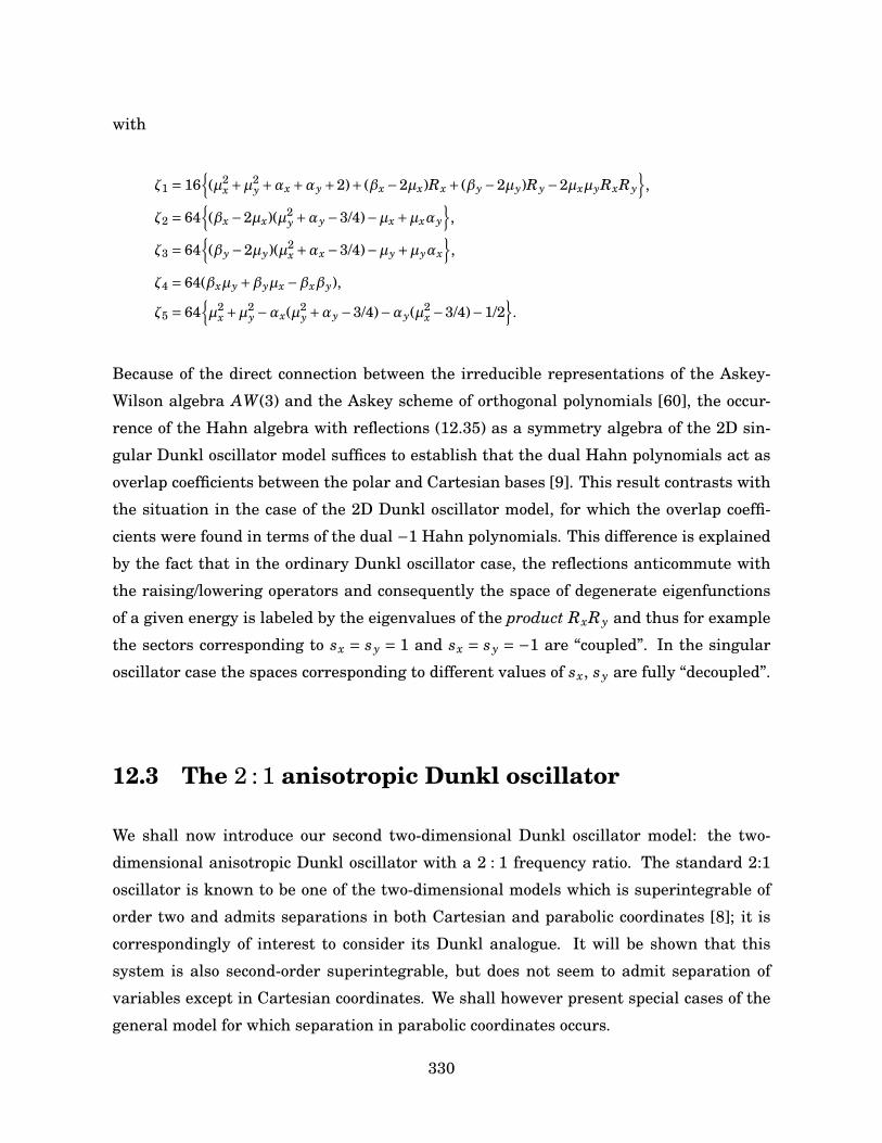
with
ζ1 = 16(µ2
x +µ2y +αx +αy +2)+ (βx −2µx)Rx + (βy −2µy)Ry −2µxµyRxRy
,
ζ2 = 64(βx −2µx)(µ2
y +αy −3/4)−µx +µxαy
,
ζ3 = 64(βy −2µy)(µ2
x +αx −3/4)−µy +µyαx
,
ζ4 = 64(βxµy +βyµx −βxβy),
ζ5 = 64µ2
x +µ2y −αx(µ2
y +αy −3/4)−αy(µ2x −3/4)−1/2
.
Because of the direct connection between the irreducible representations of the Askey-
Wilson algebra AW(3) and the Askey scheme of orthogonal polynomials [60], the occur-
rence of the Hahn algebra with reflections (12.35) as a symmetry algebra of the 2D sin-
gular Dunkl oscillator model suffices to establish that the dual Hahn polynomials act as
overlap coefficients between the polar and Cartesian bases [9]. This result contrasts with
the situation in the case of the 2D Dunkl oscillator model, for which the overlap coeffi-
cients were found in terms of the dual −1 Hahn polynomials. This difference is explained
by the fact that in the ordinary Dunkl oscillator case, the reflections anticommute with
the raising/lowering operators and consequently the space of degenerate eigenfunctions
of a given energy is labeled by the eigenvalues of the product RxRy and thus for example
the sectors corresponding to sx = sy = 1 and sx = sy = −1 are “coupled”. In the singular
oscillator case the spaces corresponding to different values of sx, sy are fully “decoupled”.
12.3 The 2 : 1 anisotropic Dunkl oscillator
We shall now introduce our second two-dimensional Dunkl oscillator model: the two-
dimensional anisotropic Dunkl oscillator with a 2 : 1 frequency ratio. The standard 2:1
oscillator is known to be one of the two-dimensional models which is superintegrable of
order two and admits separations in both Cartesian and parabolic coordinates [8]; it is
correspondingly of interest to consider its Dunkl analogue. It will be shown that this
system is also second-order superintegrable, but does not seem to admit separation of
variables except in Cartesian coordinates. We shall however present special cases of the
general model for which separation in parabolic coordinates occurs.
330
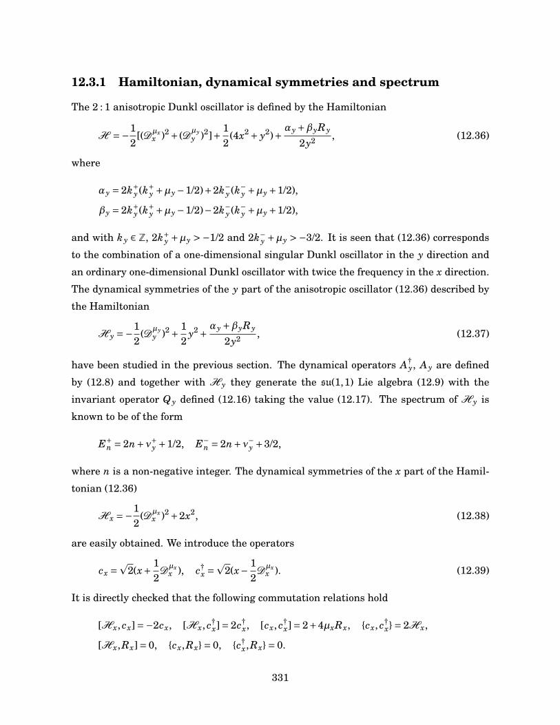
12.3.1 Hamiltonian, dynamical symmetries and spectrum
The 2 : 1 anisotropic Dunkl oscillator is defined by the Hamiltonian
H =−12
[(Dµxx )2 + (Dµy
y )2]+ 12
(4x2 + y2)+ αy +βyRy
2y2 , (12.36)
where
αy = 2k+y (k+
y +µy −1/2)+2k−y (k−
y +µy +1/2),
βy = 2k+y (k+
y +µy −1/2)−2k−y (k−
y +µy +1/2),
and with ky ∈ Z, 2k+y +µy >−1/2 and 2k−
y +µy >−3/2. It is seen that (12.36) corresponds
to the combination of a one-dimensional singular Dunkl oscillator in the y direction and
an ordinary one-dimensional Dunkl oscillator with twice the frequency in the x direction.
The dynamical symmetries of the y part of the anisotropic oscillator (12.36) described by
the Hamiltonian
H y =−12
(Dµyy )2 + 1
2y2 + αy +βyRy
2y2 , (12.37)
have been studied in the previous section. The dynamical operators A†y, A y are defined
by (12.8) and together with H y they generate the su(1,1) Lie algebra (12.9) with the
invariant operator Q y defined (12.16) taking the value (12.17). The spectrum of H y is
known to be of the form
E+n = 2n+ν+y +1/2, E−
n = 2n+ν−y +3/2,
where n is a non-negative integer. The dynamical symmetries of the x part of the Hamil-
tonian (12.36)
Hx =−12
(Dµxx )2 +2x2, (12.38)
are easily obtained. We introduce the operators
cx =p
2(x+ 12
Dµxx ), c†
x =p
2(x− 12
Dµxx ). (12.39)
It is directly checked that the following commutation relations hold
[Hx, cx]=−2cx, [Hx, c†x]= 2c†
x, [cx, c†x]= 2+4µxRx, cx, c†
x= 2Hx,
[Hx,Rx]= 0, cx,Rx= 0, c†x,Rx= 0.
331
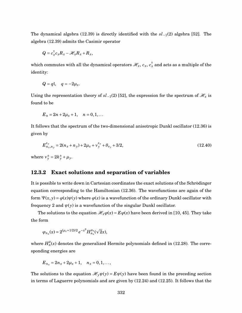
The dynamical algebra (12.39) is directly identified with the sl−1(2) algebra [52]. The
algebra (12.39) admits the Casimir operator
Q = c†xcxRx −HxRx +Rx,
which commutes with all the dynamical operators Hx, cx, c†x and acts as a multiple of the
identity:
Q = qI, q =−2µx.
Using the representation theory of sl−1(2) [52], the expression for the spectrum of Hx is
found to be
En = 2n+2µx +1, n = 0,1, . . .
It follows that the spectrum of the two-dimensional anisotropic Dunkl oscillator (12.36) is
given by
Esynx,ny = 2(nx +ny)+2µx +νsy
y +θsy +3/2, (12.40)
where ν±y = 2k±y +µy.
12.3.2 Exact solutions and separation of variables
It is possible to write down in Cartesian coordinates the exact solutions of the Schrödinger
equation corresponding to the Hamiltonian (12.36). The wavefunctions are again of the
form Ψ(x, y)=ϕ(x)ψ(y) where ϕ(x) is a wavefunction of the ordinary Dunkl oscillator with
frequency 2 and ψ(y) is a wavefunction of the singular Dunkl oscillator.
The solutions to the equation Hxϕ(x)= Eϕ(x) have been derived in [10, 45]. They take
the form
ϕnx(x)= 2(µx+1/2)/2 e−x2Hµx
nx(p
2x),
where Hµn(x) denotes the generalized Hermite polynomials defined in (12.28). The corre-
sponding energies are
Enx = 2nx +2µx +1, nx = 0,1, . . . ,
The solutions to the equation H yψ(y) = Eψ(y) have been found in the preceding sectionin terms of Laguerre polynomials and are given by (12.24) and (12.25). It follows that the
332
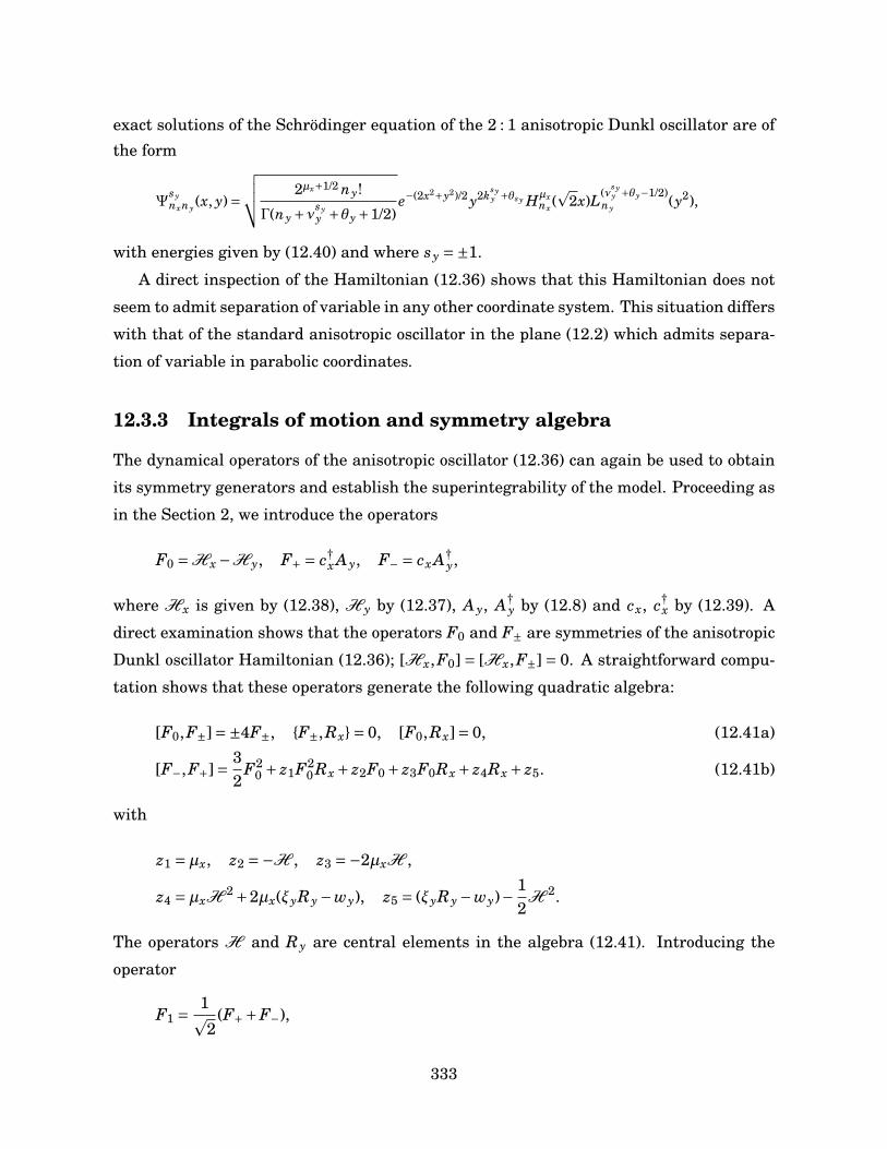
exact solutions of the Schrödinger equation of the 2 : 1 anisotropic Dunkl oscillator are ofthe form
Ψsynxny(x, y)=
√√√√ 2µx+1/2 ny!
Γ(ny +νsyy +θy +1/2)
e−(2x2+y2)/2 y2ksyy +θsy Hµx
nx (p
2x)L(νsyy +θy−1/2)
ny (y2),
with energies given by (12.40) and where sy =±1.
A direct inspection of the Hamiltonian (12.36) shows that this Hamiltonian does not
seem to admit separation of variable in any other coordinate system. This situation differs
with that of the standard anisotropic oscillator in the plane (12.2) which admits separa-
tion of variable in parabolic coordinates.
12.3.3 Integrals of motion and symmetry algebra
The dynamical operators of the anisotropic oscillator (12.36) can again be used to obtain
its symmetry generators and establish the superintegrability of the model. Proceeding as
in the Section 2, we introduce the operators
F0 =Hx −H y, F+ = c†x A y, F− = cx A†
y,
where Hx is given by (12.38), H y by (12.37), A y, A†y by (12.8) and cx, c†
x by (12.39). A
direct examination shows that the operators F0 and F± are symmetries of the anisotropic
Dunkl oscillator Hamiltonian (12.36); [Hx,F0] = [Hx,F±] = 0. A straightforward compu-
tation shows that these operators generate the following quadratic algebra:
[F0,F±]=±4F±, F±,Rx= 0, [F0,Rx]= 0, (12.41a)
[F−,F+]= 32
F20 + z1F2
0 Rx + z2F0 + z3F0Rx + z4Rx + z5. (12.41b)
with
z1 =µx, z2 =−H , z3 =−2µxH ,
z4 =µxH2 +2µx(ξyRy −wy), z5 = (ξyRy −wy)− 1
2H 2.
The operators H and Ry are central elements in the algebra (12.41). Introducing the
operator
F1 = 1p2
(F++F−),
333
one finds that
F1 = 12
Dµyy , (xD
µyy − yD
µxx )+ xy2 − x
y2 (αy +βyRy), (12.42)
where x, y = xy+ yx. The operator F1 is thus seen to be a Dunkl analogue of the gen-
eralized Runge-Lenz vector [15], which is the symmetry associated to the separation of
variables in parabolic coordinates in the standard anisotropic oscillator case. The Dunkl
Hamiltonian (12.36) does not however separate in this coordinate system due to the pres-
ence of singular terms in both the x and y parts.
We shall now examine two special cases of the 2 : 1 anisotropic Dunkl oscillator for
which the separation in parabolic coordinates is however possible. These special cases are
obtained by removing the reflections in the x-part (12.38) which prevents the separation
in parabolic coordinates.
12.3.4 Special case I
The first special case of the 2 : 1 anisotropic Dunkl oscillator that we consider is described
by the Hamiltonian
H I =−12
[∂2x + (Dµy
y )2]+ 12
(4x2 + y2)+ αy +βyRy
2y2 , (12.43)
with the usual quantization conditions
αy = 2k+y (k+
y +µy −1/2)+2k−y (k−
y +µy +1/2),
βy = 2k+y (k+
y +µy −1/2)−2k−y (k−
y +µy +1/2),
where ky ∈ Z. It is easily seen that this Hamiltonian is obtained from (12.36) by taking
µx = 0 and hence it is superintegrable and its symmetry algebra is obtained directly from
(12.41). Moreover, the Hamiltonian (12.43) corresponds to the combination of a standard
harmonic oscillator in the x direction with a singular Dunkl oscillator in the y direction.
In parabolic coordinates
x = 12
(u2 −v2), y= uv,
the Schrödinger equation H IΨ(u,v) = EΨ(u,v), where H I is the Hamiltonian given by
(12.43), takes the form
[Cu +Cv]Ψ(u,v)=−2E(u2 +v2)Ψ(u,v),
334
where
Cu = ∂2u +
2µy
u∂u −
µy
u2 (1−Ry)− 1u2 (αy +βyRy)−u6.
Since the reflection operator Ry commutes with H I , the wavefunctionΨ(u,v) can be taken
to have a definite parity. In the even sector, defined by the relation RyΨ+(u,v)=Ψ+(u,v),
the separation Ansatz Ψ+(u,v) =U(u)V (v) yields the following pair of ordinary differen-
tial equations:
U ′′(u)+ 2µy
uU ′(u)+
2Eu2 − αy +βy
u2 −u6
U(u)=Λ+U(u), (12.44a)
V ′′(v)+ 2µy
vV ′(v)+
2Ev2 − αy +βy
v2 −v6
V (v)=−Λ+V (v), (12.44b)
where Λ+ is the separation constant. Upon imposing the condition U(−u) = U(u), the
solution to the equation (12.44a) is seen to be given by
U+(u)= e−u4/4u2k+y B(ν+y −1/2;0;E;
Λ+p
2;
u2p
2),
where B(α;β;γ;δ; z) is the Heun biconfluent function. The Heun biconfluent function is
defined as the solution to the differential equation
B′′(z)− (−α+βz+2z2 −1)z
B′(z)− 12
(αβ+β+δ+ z(2α+4−2γ))z
B(z)= 0,
with initial conditions B(0)= 1 and B′(0)= (αβ+β+δ)/(2α+2). Similarly, the solution for
V (v) is directly given by
V+(v)= e−v4/4v2k+y B(ν+y −1/2;0;E;
−Λ+p
2;
v2p
2).
In the odd sector, defined by the relation RyΨ(u,v)=−Ψ(u,v), we obtain
U−(u)= e−u4/4u2k−y+1 B(ν−y +1/2;0;E;
Λ−p
2;
u2p
2),
and
V−(v)= e−v4/4u2k−y+1 B(ν−y +1/2;0;E;
−Λ−p
2;
v2p
2).
In parabolic coordinates, the operator F1 given in (12.42) can readily be shown to be
diagonal and its eigenvalues can be related to the separation constants Λ±. As is the case
for the standard anisotropic oscillator (12.2), the parameters Λ obey a transcendental
equation and cannot be expressed explicitly [33].
335
12.3.5 Special case II
Another special case of the 2 : 1 anisotropic Dunkl oscillator which admits separation of
variables in parabolic coordinates is described by the Hamiltonian
H I I =−12
[∂2x + (Dµy
y )2]+ 12
(4x2 + y2). (12.45)
The Hamiltonian (12.45) is obtained by taking µx = 0, αy = 0 and βy = 0 in (12.36). It
corresponds to the combination of an ordinary Dunkl oscillator in the y direction and a
standard oscillator with twice the frequency in the x direction. For this Hamiltonian, the
symmetry algebra is not a special case of the algebra (12.41); this follows from the fact
that the dynamical operators of the singular Dunkl oscillator involve the squares of the
dynamical symmetries of the ordinary Dunkl oscillator.
The dynamical operators in the present special case are rather the creation and anni-
hilation operators of the standard oscillator
gx =p
2(x+ 12∂x), g†
x =p
2(x− 12∂x),
which are part of the algebra
[gx, g†x]= 2, [Hx, gx]=−2gx, [Hx, g†
x]= 2g†x,
and those of the one-dimensional Dunkl (or parabosonic) oscillator
hy = 1p2
(y+Dµyy ), h†
y =1p2
(y−Dµyy ),
which obey the sl−1(2) algebra relations
[hy,h†y]= 1+2µyRy, [H y,hy]=−hy, [H y,h†
y]= h†y.
The symmetries of the Hamiltonian (12.45) are of the form
T0 =Hx −H y, T+ = g†xhy, T− = gxh†
y,
and they generate the following algebra:
[T0,T±]=±3T±, T±,Ry= 0, [T0,Ry]= 0,
[T+,T−]= 32
T0 +µyT0Ry +H (µyRy −1/2)+2µyRy.
Similarly to the preceding special case, the separation of variable in parabolic coordinates
can be performed and the wavefunctions in these coordinates satisfy the biconfluent Heun
equation. Since the computations are analogous to those already presented here, we omit
the details.
336

12.4 Conclusion
In this paper, we have considered two extensions of the Dunkl oscillator model: one with
additional singular terms in the potential and the other with singular terms and a 2 : 1
frequency ratio. We showed that the singular Dunkl oscillator is second-order superinte-
grable and exhibited its symmetry generators. We also identified the symmetry algebra
as an extension with central involution operators of a special case of the Askey-Wilson
algebra AW(3). We also obtained the exact solutions in both Cartesian and polar coordi-
nates. For the 2 : 1 anisotropic Dunkl oscillator, we showed the system to be also second-
order superintegrable, exhibited the symmetries and obtained the algebra they generate.
Special cases for which separation of variables in parabolic coordinates occurs were also
considered and their symmetry algebras found. In one instance, it was shown that the
wavefunctions in parabolic coordinates obey the biconfluent Heun equation.
The models investigated here can be considered as generalizations of the standard
singular oscillator (12.1) and 2 : 1 anisotropic oscillator (12.2) with the derivatives re-
placed by the Dunkl derivatives. In this context, it is natural to consider the Hamiltonian
corresponding to the Dunkl-Coulomb problem
H =−12∇2
D + α
r,
where ∇2D
is the Dunkl-Laplacian, which in Cartesian coordinates reads
∇2D = (Dµx
x )2 + (Dµyy )2.
The spectrum of this Hamiltonian can be evaluated algebraically using the observation
that r, r∇2D
and x∂x + y∂y obey the sl2 relations [4]. The expression for the values of the
energy then depend on a single quantum number and the spectrum of H exhibits acciden-
tal degeneracies; this suggests that the Dunkl-Coulomb Hamiltonian in the plane is also
superintegrable. In the standard case, it is known that the singular oscillator model (12.1)
can be related to the Coulomb problem via the Levi-Civita mapping. This is not so with
the singular Dunkl oscillator and Dunkl-Coulomb problem since the Levi-Civita map-
ping amounts to a passage from Cartesian to parabolic coordinates, a coordinate system
in which the Dunkl Laplacian does not separate. Hence the Dunkl-Coulomb problem is
genuinely different from the singular Dunkl oscillator and shall be considered elsewhere.
It would be of interest in a future study to identify and characterize other novel su-
perintegrable systems of Dunkl type. The Dunkl-type models defined on the circle, in the
337
3-dimensional Euclidean space and on the 2-sphere are of particular interest. Given the
relation of Dunkl oscillator models and −1 polynomials, this study could provide further
insight into the emerging Bannai-Ito scheme of −1 orthogonal polynomials.
References
[1] Makarov A., Y. A. Smorodinsky, Valiev K., and P. Winternitz. A systematic search for nonrel-
ativistic systems with dynamical symmetries. Nuovo Cimentos, 52:1061–1084, 1967.
[2] F. Calogero. Solutions of a three-body problem in one-dimension. Journal of Mathematical
Physics, 10:2191–2196, 1969.
[3] T. Chihara. An Introduction to Orthogonal Polynomials. Gordon and Breach, New-York,
1978.
[4] H. De Bie, B. Orsted, P. Somberg, and V. Soucek. Dunkl operators and a family of realizations
of osp(1|2). Transactions of the American Mathematical Society, 364:3875–3902, 2012.
[5] C.F. Dunkl. Differential-Difference operators associated to reflection groups. Transactions of
the American Mathematical Society, 311:167–183, 1989.
[6] C.F. Dunkl and Y. Xu. Orthogonal polynomials of several variables. Cambridge University
Press, 2001.
[7] R. Floreanini, L. Lapointe, and L. Vinet. The polynomial SU(2) symmetry algebra of the
two-body Calogero model. Physics Letters B, 389:327–333, 1996.
[8] I. Fris, V. Mandrosov, Y. A. Smorodinsky, M. Ulhìr, and P. Winternitz. On higher symmetries
in quantum mechanics. Physics Letters, 16:354–356, 1965.
[9] O.F. Gal’bert, Y. Granovskii, and A. Zhedanov. Dynamical symmetry of anisotropic singular
oscillator. Physics Letters A, 153:177–180, 1991.
[10] V.X. Genest, M. E. H. Ismail, L. Vinet, and A. Zhedanov. The Dunkl oscillator in the plane: I.
Superintegrability, separated wavefunctions and overlap coefficients. Journal of Physics A:
Mathematical and Theoretical, 46:145201, 2013.
[11] V.X. Genest, M. E. H. Ismail, L. Vinet, and A. Zhedanov. The Dunkl oscillator in the plane:
II. Representations of the symmetry algebra. Communications in Mathematical Physics,
329:999-1029, 2014.
338

[12] V.X. Genest, L. Vinet, and A. Zhedanov. Bispectrality of the Complementary Bannai-Ito
polynomials. SIGMA, 9:18–38, 2013.
[13] V.X. Genest, L. Vinet, and A. Zhedanov. The algebra of dual −1 Hahn polynomials and the
Clebsch-Gordan problem of sl−1(2). Journal of Mathematical Physics, 54:023506, 2013.
[14] V.X. Genest, L. Vinet, and A. Zhedanov. The Bannai-Ito polynomials as Racah coefficients of
the sl−1(2) algebra. Proceedings of the American Mathematical Society, 142:1545-1560, 2014.
[15] H. Goldstein. Classical Mechanics. Addison-Wesley, 2nd edition, 1980.
[16] Y. Granovskii, A. Zhedanov, and I. Lutsenko. Mutual integrability, quadratic algebras and
dynamical symmetry. Annals of Physics, 217:1–20, 1992.
[17] Y. Granovskii, A. Zhedanov, and I. Lutsenko. Quadratic algebras and dynamics in curved
spaces I. Oscillator. Theoretical and Mathematical Physics, 91:474–480, 1992.
[18] Y. Granovskii, A. Zhedanov, and I. Lutsenko. Quadratic algebras and dynamics in curved
spaces II. The Kepler problem. Theoretical and Mathematical Physics, 91:604–612, 1992.
[19] J.E. Humphreys. Introduction to Lie algebras and representation theory. Springer Verlag,
1972.
[20] Minahan J.A. and Polychronakos A.P. Integrable systems for particles with internal degrees
of freedom. Physics Letters B, 302:265–270, 1993.
[21] E.I. Jafarov, N.I. Stoilova, and J. Van der Jeugt. The su(2)α Hahn oscillator and a discrete
Hahn-Fourier transform. Journal of Physics A: Mathematical and Theoretical, 44:355205,
2011.
[22] E.I. Jafarov, N.I. Stoilova, and J. Van der Jeugt. Deformed su(1,1) algebra as a model for
Quantum Oscillators. SIGMA, 8:025, 2012.
[23] E.G. Kalnins, J.M. Kress, and W. Jr. Miller. Second order superintegrable systems in con-
formally flat spaces. I. 2D classical structure theory. Journal of Mathematical Physics,
46:053509, 2005.
[24] E.G. Kalnins, J.M. Kress, and W. Jr. Miller. Second order superintegrable systems in con-
formally flat spaces. V. 2D and 3D quantum systems. Journal of Mathematical Physics,
46:093501, 2006.
[25] E.G. Kalnins, J.M. Kress, and W. Jr. Miller. A recurrence relation approach to higher order
quantum superintegrability. SIGMA, 7:31–55, 2011.
339
[26] E.G. Kalnins and W. Jr. Miller. Structure results for higher order symmetry algebras of 2D
classical superintegrable systems. Journal of Nonlinear Systems and Applications, pages
29–40, 2012.
[27] E.G. Kalnins, W. Jr. Miller, and G.S. Pogosyan. Superintegrability and associated polyno-
mial solutions: Euclidian space and the sphere in two dimensions. Journal of Mathematical
Physics, 37:6439, 1996.
[28] E.G. Kalnins, W. Jr. Miller, and S. Post. Models for Quadratic Algebras Associated with
Second Order Superintegrable Systems in 2D. SIGMA, 4:8–28, 2008.
[29] E.G. Kalnins, W. Jr. Miller, and S. Post. Contractions of 2D 2nd order superintegrable systems
and the Askey scheme for hypergeometric orthogonal polynomials. Arxiv, 2013.
[30] R. Koekoek, P.A. Lesky, and R.F. Swarttouw. Hypergeometric orthogonal polynomials and
their q-analogues. Springer, 1st edition, 2010.
[31] Brink L., Hansson T.H., Konstein S., and Vasiliev M.A. The Calogero model: anyonic presen-
tations, fermionic extension and supersymmetry. Nuclear Physics B, 401:591–612, 1993.
[32] L. Lapointe and L. Vinet. Exact operator solutions of the Calogero-Sutherlad model. Com-
munications in Mathematical Physics, 178:425–452, 1996.
[33] P. Létourneau and L. Vinet. Superintegrable systems: polynomial algebras and quasi-exactly
solvable hamiltonians. Annals of Physics, 243:144–168, 1995.
[34] I. Marquette. Construction of classical superintegrable systems with higher order integrals
of motion from ladder operators. Journal of Mathematical Physics, 51:072903, 2010.
[35] I. Marquette and C. Quesne. New families of superintegrable systems from Hermite and
Laguerre exceptional orthogonal polynomials. Journal of Mathematical Physics, 54:042102,
2013.
[36] H. Miki, S. Post, L. Vinet, and A. Zhedanov. A superintegrable finite oscillator in two dimen-
sions with SU(2) symmetry. Arxiv, 2012.
[37] W. Jr. Miller. Symmetry and Separation of Variables. Addison-Wesley, 1977.
[38] N. Mukunda, E.C.G. Sudarshan, J.K. Sharma, and C.L. Mehta. Representations and proper-
ties of para-Bose oscillator operators I. Energy position and momentum eigenstates. Journal
of Mathematical Physics, 21:2386–2394, 1980.
[39] P. J. Olver. Applications of Lie groups to differential equations. Springer, 1993.
340
[40] M.S. Plyushchay. R-deformed Heisenberg algebras. Modern Physics Letters A, 11:2953–2964,
1996.
[41] M.S. Plyushchay. Deformed Heisenberg algebra with reflection. Nuclear Physics B, 491:619–
634, 1997.
[42] S. Post, S. Tsujimoto, and L. Vinet. Families of superintegrable Hamiltonians con-
structed from exceptional polynomials. Journal of Physics A: Mathematical and Theoretical,
45:405202, 2012.
[43] S. Post, S. Tsujimoto, and L. Vinet. Families of superintegrable Hamiltonians con-
structed from exceptional polynomials. Journal of Physics A: Mathematical and Theoretical,
45:405202, 2012.
[44] S. Post, L. Vinet, and A. Zhedanov. An infinite family of superintegrable Hamiltonians with
reflection in the plane. Journal of Physics A: Mathematical and Theoretical, 44:505201, 2011.
[45] M. Rosenblum. Generalized Hermite polynomials and the Bose-like oscillator calculus. In
Operator Theory: Advances and Applications, 1994.
[46] M. Rösler. Dunkl operators: theory and applications. In Lecture notes in Mathematics.
Springer, 2002.
[47] J.K. Sharma, C.L. Mehta, N. Mukunda, and E.C.G. Sudarshan. Representations and proper-
ties of para-Bose oscillators II. Coherent states and the minimum uncertainty states. Journal
of Mathematical Physics, 22:78–90, 1981.
[48] B. Sutherland. Quantum many-body problem in one dimension. Journal of Mathematical
Physics, 12:246–250, 1971.
[49] Baker T.H., C.F. Dunkl, and J.P. Forrester. Polynomial eigenfunctions of the Calogero-
Sutherland-Moser models with exchange terms. In J. F. van Diejen and L. Vinet, editors,
Calogero-Sutherland-Moser models, CRM Series in Mathematical Physics. Springer, 2000.
[50] F. Tremblay, A. Turbiner, and P. Winternitz. An infinite family of solvable and inte-
grable quantum systems in the plane. Journal of Physics A: Mathematical and Theoretical,
42:242001, 2009.
[51] F. Tremblay, A. Turbiner, and P. Winternitz. Periodic orbits for an infinite family of classical
superintegrable systems. Journal of Physics A: Mathematical and Theoretical, 43:015202,
2010.
341

[52] S. Tsujimoto, L. Vinet, and A. Zhedanov. From slq(2) to a parabosonic Hopf algebra. SIGMA,
7:93–106, 2011.
[53] S. Tsujimoto, L. Vinet, and A. Zhedanov. Jordan algebras and orthogonal polynomials. Jour-
nal of Mathematical Physics, 52:103512, 2011.
[54] S. Tsujimoto, L. Vinet, and A. Zhedanov. Dual −1 Hahn polynomials: "classical" polynomials
beyond the Leonard duality. Proceedings of the American Mathematical Society, 141:959–
970, 2012.
[55] S. Tsujimoto, L. Vinet, and A. Zhedanov. Dunkl shift operators and Bannai-Ito polynomials.
Advances in Mathematics, 229:2123–2158, 2012.
[56] L. Vinet and A. Zhedanov. A ’missing’ family of classical orthogonal polynomials20. Journal
of Physics A: Mathematical and Theoretical, 44:085201, 2011.
[57] L. Vinet and A. Zhedanov. A limit q = −1 for the Big q-Jacobi polynomials. Transactions of
the American Mathematical Society, 364:5491–5507, 2012.
[58] L. Vinet and A. Zhedanov. Para-Krawtchouk polynomials on a bi-lattice and a quantum
spin chain with perfect state transfer. Journal of Physics A: Mathematical and Theoretical,
45:265304, 2012.
[59] P. Winternitz, Y. A. Smorodinsky, M. Ulhìr, and I. Fris. Symmetry groups in classical and
quantum mechanics. Soviet Journal of Nuclear Physics, 4:444–450, 1967.
[60] A. Zhedanov. Hidden symmetry of Askey-Wilson polynomials. Theoreticheskaya i Matem-
aticheskaya Fizika, 89:190–204, 1991.
342
Chapitre 13
The Dunkl oscillator in threedimensions
V. X. Genest, L. Vinet et A. Zhedanov. The Dunkl oscillator in three dimensions (2014). Journal of
Physics: Conference Series 512 012010
Abstract. The isotropic Dunkl oscillator model in three-dimensional Euclidean space is consid-
ered. The system is shown to be maximally superintegrable and its symmetries are obtained by
the Schwinger construction using the raising/lowering operators of the dynamical sl−1(2) algebra
of the one-dimensional Dunkl oscillator. The invariance algebra generated by the constants of
motion, an extension of u(3) with reflections, is called the Schwinger-Dunkl algebra sd(3). The
system is shown to admit separation of variables in Cartesian, polar (cylindrical) and spherical
coordinates and the corresponding separated solutions are expressed in terms of generalized Her-
mite, Laguerre and Jacobi polynomials.
13.1 Introduction
This paper is concerned with the study of the isotropic Dunkl oscillator model in three-dimensional
Euclidean space. This model, described by a Hamiltonian involving reflection operators, will be
shown to be both maximally superintegrable and exactly solvable. The constants of motion will
be obtained by the Schwinger construction using the sl−1(2) dynamical symmetry of the parabose
oscillator in one dimension. The invariance algebra generated by the symmetries will be seen to
be an extension of u(3) by involutions and shall be called the Schwinger-Dunkl algebra sd(3). The
Schrödinger equation of the system will be seen to admit separation of variables in Cartesian,
polar (cylindrical) and spherical coordinates. The corresponding separated solutions will be found
343
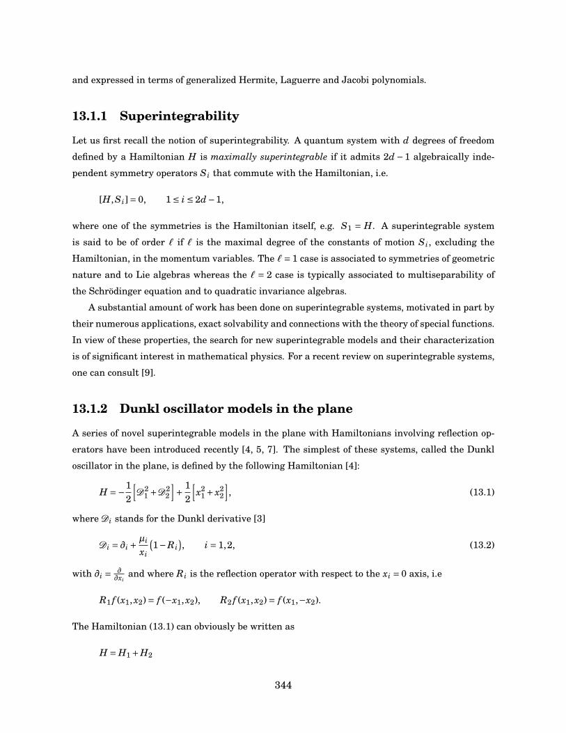
and expressed in terms of generalized Hermite, Laguerre and Jacobi polynomials.
13.1.1 Superintegrability
Let us first recall the notion of superintegrability. A quantum system with d degrees of freedom
defined by a Hamiltonian H is maximally superintegrable if it admits 2d −1 algebraically inde-
pendent symmetry operators Si that commute with the Hamiltonian, i.e.
[H,Si]= 0, 1≤ i ≤ 2d−1,
where one of the symmetries is the Hamiltonian itself, e.g. S1 = H. A superintegrable system
is said to be of order ` if ` is the maximal degree of the constants of motion Si, excluding the
Hamiltonian, in the momentum variables. The `= 1 case is associated to symmetries of geometric
nature and to Lie algebras whereas the ` = 2 case is typically associated to multiseparability of
the Schrödinger equation and to quadratic invariance algebras.
A substantial amount of work has been done on superintegrable systems, motivated in part by
their numerous applications, exact solvability and connections with the theory of special functions.
In view of these properties, the search for new superintegrable models and their characterization
is of significant interest in mathematical physics. For a recent review on superintegrable systems,
one can consult [9].
13.1.2 Dunkl oscillator models in the plane
A series of novel superintegrable models in the plane with Hamiltonians involving reflection op-
erators have been introduced recently [4, 5, 7]. The simplest of these systems, called the Dunkl
oscillator in the plane, is defined by the following Hamiltonian [4]:
H =−12
[D2
1 +D22
]+ 1
2
[x2
1 + x22
], (13.1)
where Di stands for the Dunkl derivative [3]
Di = ∂i + µi
xi
(1−Ri
), i = 1,2, (13.2)
with ∂i = ∂∂xi
and where Ri is the reflection operator with respect to the xi = 0 axis, i.e
R1 f (x1, x2)= f (−x1, x2), R2 f (x1, x2)= f (x1,−x2).
The Hamiltonian (13.1) can obviously be written as
H = H1 +H2
344

where Hi, i = 1,2, is the one-dimensional Dunkl oscillator Hamiltonian
Hi =−12
D2i +
12
x2i . (13.3)
In [4], the Hamiltonian (13.1) was shown to be maximally superintegrable and its two independent
constants of motion, obtained by the Schwinger construction, were seen to generate a u(2) algebra
extended with involutions. This algebra was called the Schwinger-Dunkl algebra sd(2). It was
further shown that the Schrödinger equation associated to (13.1) admits separation of variables in
both Cartesian and polar coordinates and the separated wavefunctions were given explicitly. Fur-
thermore, the overlap coefficients between the separated wavefunctions were expressed in terms
of the dual −1 Hahn polynomials through a correspondence with the Clebsch-Gordan problem of
sl−1(2), a q →−1 limit of the quantum algebra slq(2) (see Section II for the definition of sl−1(2) and
[11] for background). In [5], the representation theory of the Schwinger-Dunkl algebra sd(2) was
examined. The results obtained in this paper further strengthened the idea that Dunkl oscillator
models are showcases for −1 orthogonal polynomials (see [6, 12]).
Generalizations of the Dunkl oscillator in the plane (13.1) were considered in [7], where the
singular and the 2 : 1 anisotropic Dunkl oscillators were investigated. The two systems were
shown to be superintegrable, their constants of motion were constructed and their (quadratic)
invariance algebra was given. It was also shown that in some cases these models exhibit mul-
tiseparability. Here we pursue our investigations on Dunkl oscillator models by considering the
three-dimensional version of the system (13.1) in Euclidean space.
13.1.3 The three-dimensional Dunkl oscillator
The Dunkl oscillator in three-dimensional Euclidean space is defined by the Hamiltonian
H =−12
[D2
1 +D22 +D2
3
]+ 1
2
[x2
1 + x22 + x2
3
], (13.4)
where Di is the Dunkl derivative given by (13.2). An elementary calculation shows that the square
of the Dunkl derivative has the expression
D2i = ∂2
i +2µi
xi∂i − µi
x2i
(1−Ri).
As is directly seen, the Hamiltonian (13.4) corresponds to the combination of three independent
(commuting) one-dimensional Dunkl oscillators with Hamiltonians Hi given by (13.3). It directly
follows from the formulas (13.2) and (13.4) that when µi = 0, i = 1,2,3, the Dunkl oscillator Hamil-
tonian (13.4) reduces to that of the standard isotropic harmonic oscillator in three dimensions. We
note that the term “isotropic” here refers to the fact that the three independent one-dimensional
oscillator entering the total Hamiltonian (13.4) have the same frequency. To obtain a 3D Dunkl
oscillator isotropic in the sense of being O(3)-invariant, one must also take µ1 =µ2 =µ3.
345
13.1.4 Outline
The paper is organized in the following way. In section II, the sl−1(2) dynamical symmetry and
the Schwinger construction are used to obtain the symmetries of the total Hamiltonian (13.4),
thus establishing its superintegrability. The commutation relations satisfied by the constants
of motion, which define the Schwinger-Dunkl algebra sd(3), are also exhibited in two different
bases. In section III, the separated solutions of the Schrödinger equation associated to (13.4) are
given in Cartesian, polar and spherical coordinates. For each coordinate system, the symmetries
responsible for the separation of variables are given. A short conclusion follows.
13.2 Superintegrability
In this section, the sl−1(2) dynamical algebra of the three-dimensional Dunkl oscillator is made
explicit and is exploited to obtain the spectrum of the Hamiltonian. Following the Schwinger
construction, the constants of motion are constructed using the raising/lowering operators of the
sl−1(2) algebra of the one-dimensional constituents. The Schwinger-Dunkl algebra sd(3) formed
by the symmetries is seen to correspond to a deformation of the Lie algebra u(3) by involutions
and the defining relations of sd(3) are given in two different bases.
13.2.1 Dynamical algebra and spectrum
The three-dimensional Dunkl oscillator Hamiltonian (13.4) possesses an sl−1(2) dynamical sym-
metry inherited from the one of its one-dimensional constituents Hi. This can be seen as follows.
Consider the following operators:
A(i)± = 1p
2
(xi ∓Di
), (13.5)
and define A(i)0 = Hi with Hi given by (13.3). It is easily checked that these operators, together
with the reflection operator Ri, satisfy the defining relations of the sl−1(2) algebra which are of
the form [11]
[A(i)0 , A(i)
± ]=±A(i)± , [A(i)
0 ,Ri]= 0, A(i)+ , A(i)
− = 2A(i)0 , A(i)
± ,Ri= 0, (13.6)
where [x, y] = xy− yx and x, y = xy+ yx. As is seen from the above commutation relations, the
operators A(i)± act as raising/lowering operators for the one-dimensional Hamiltonians A(i)
0 = Hi.
In the realization (13.5), the sl−1(2) Casimir operator
Q(i) = A(i)+ A(i)
− Ri − A(i)0 Ri +Ri/2,
346

is a multiple of the identity Q(i) =−µi. It thus follows that for µi >−1/2, the operators A(i)± , A(i)
0 and
Ri realize the positive-discrete series of representations of sl−1(2) [11]. In these representations,
the spectrum E (i) of the operators A(i)0 is given by
E (i)ni
= ni +µi +1/2,
where ni is a non-negative integer. Given that the full Hamiltonian (13.4) of the three-dimensional
Dunkl oscillator is of the form H = H1+H2+H3, it follows that its energy eigenvalues E have the
expression
EN = N +µ1 +µ2 +µ3 +3/2, (13.7)
where N is a non-negative integer. Since the integer N can be written as N = n1 + n2 + n3, the
spectrum of H has degeneracy
gN =N∑
n3=0(N −n3 +1)= (N +1)(N +2)/2,
at energy level EN . Hence the three-dimensional Dunkl oscillator exhibits the same degeneracy in
its spectrum as the standard three-dimensional isotropic oscillator.
The coproduct of sl−1(2) (see [11]) can be used to construct the sl−1(2) dynamical algebra of
the total Hamiltonian H . Indeed, upon defining the operators
A± = A(1)± R2R3 + A(2)
± R3 + A(3)± , R = R1R2R3, A0 =H ,
it is directly checked that one has
[A0,A±]=±A±, [A0,R]= 0, A+,A−= 2A0, A±,R= 0.
Hence the operators A± act as the raising/lowering operators for the full Hamiltonian H of the
three-dimensional Dunkl oscillator.
13.2.2 Constants of motion and
the Schwinger-Dunkl algebra sd(3)
Given that H = H1 +H2 +H3, it is clear that combining a raising operator for Hi with a lowering
operator for H j when i 6= j will result in an operator preserving the eigenspace associated to a
given energy EN , thus producing a constant of motion of the total Hamiltonian H . Moreover,
it is obvious that the one-dimensional components Hi commute with the total Hamiltonian H
and hence these one-dimensional Hamiltonians can be considered as constants of the motion.
Furthermore, it is observed that the total Hamiltonian commutes with the reflection operators
[H ,Ri]= 0, i = 1,2,3,
347
so that the reflections can be considered as symmetries. Following the Schwinger construction of
u(3) with standard creation/annihilation operators, we define
J1 = 1i(A(2)+ A(3)
− − A(2)− A(3)
+), J2 = 1
i(A(3)+ A(1)
− − A(3)− A(1)
+),
J3 = 1i(A(1)+ A(2)
− − A(1)− A(2)
+).
The operators Ji, i = 1,2,3, can be interpreted as Dunkl “rotation” generators since in terms of
Dunkl derivatives, they read
J1 = 1i(x2D3 − x3D2), J2 = 1
i(x3D1 − x1D3), J3 = 1
i(x1D2 − x2D1). (13.8)
We also introduce the operators
K1 =(A(2)+ A(3)
− + A(2)− A(3)
+), K2 =
(A(3)+ A(1)
− + A(3)− A(1)
+), K3 =
(A(1)+ A(2)
− + A(1)− A(2)
+),
which in coordinates have the expression
K1 = (x2x3 −D2D3), K2 = (x3x1 −D3D1), K3 = (x1x2 −D1D2). (13.9)
It is directly checked that the operators Ji, K i, i = 1,2,3, are symmetries of the total Dunkl oscil-
lator Hamiltonian (13.4), that is
[Ji,H ]= [K i,H ]= 0,
for i = 1,2,3. Upon writing
L1 = H1/2, L2 = H2/2, L3 = H3/2,
which satisfy H = 2L1 +2L2 +2L3, a direct computation shows that the non-zero commutation
relations between the symmetries are given by
[J j, Jk]= iε jk`J`(1+2µ`R`), [K j,Kk]=−iε jk`J`(1+2µ`R`), (13.10a)
where εi jk stands for the totally antisymmetric tensor with summation over repeated indices un-
derstood and
[J j,Kk]=−iε jk`K`(1+2µ`R`), [J j,K j]=−iε jk`Lk(1+2µ`R`), (13.10b)
for j 6= k. One also has
[J j,Lk]= ig jkK j/2, [K j,Lk]=−ig jk J j/2, (13.10c)
348
where g i j are the elements of a 3× 3 antisymmetric matrix with g12 = g23 = 1, g13 = −1. The
commutation relations involving the reflection operators are of the form
[L i,Ri]= [L j,Rk]= [Ji,Ri]= [K i,Ri]= 0, (13.10d)
J j,Rk= K j,Rk= 0, (13.10e)
where j 6= k. Hence it follows that the three-dimensional Dunkl oscillator model is maximally
superintegrable. The invariance algebra is defined by the commutation and anticommutation
relations (13.10) and we shall refer to this algebra as the Schwinger-Dunkl algebra sd(3). It is
clear from the defining relations (13.10) that the algebra sd(3) corresponds to a deformation of the
u(3) Lie algebra by involutions; the central element here is of course the total Hamiltonian H =H1 +H2 +H3. If one takes µ1 = µ2 = µ3 = 0 in the commutation relations (13.10), one recovers the
u(3) symmetry algebra of the standard isotropic harmonic oscillator in three dimensions realized
by the standard creation/annihilation operators.
13.2.3 An alternative presentation of sd(3)
The Schwinger-Dunkl algebra sd(3) obtained here can be seen as a “rank two” version of the
Schwinger-Dunkl algebra sd(2) which has appeared in [4] as the symmetry algebra of the Dunkl
oscillator in the plane. It is possible to present another basis for the symmetries of the three-
dimensional Dunkl oscillator in which the sd(2) algebra explicitly appears as a subalgebra of
sd(3). In order to define this basis, it is convenient to introduce the standard 3×3 Gell-Mann
matrices [1] denoted by Λi, i = 1, . . . ,8, and obeying the su(3) commutation relations
[Λi,Λ j]= i f i jkΛk,
with f 123 = 2, f 458 = f 678 =p3 and
f 147 = f 165 = f 246 = f 257 = f 345 = f 376 = 1.
The symmetries of the three-dimensional Dunkl oscillator can be expressed in terms of these
matrices as follows. One takes
M j = (A(1)+ , A(2)
+ , A(3)+ )Λ j (A(1)
− , A(2)− , A(3)
− )t, (13.11)
for j = 1,2,4,5,6,7 and also
M3 = 14
(A(1)
+ , A(1)− − A(2)
+ A(2)−
),
M8 = 1
4p
3
(A(1)
+ , A(1)− + A(2)
+ , A(2)− −2A(3)
+ , A(3)−
).
349
It is straightforward to verify that the operators Mi, i = 1, . . . ,8 commute with the Hamiltonian H
of the three-dimensional Dunkl oscillator. Using the commutation relations (13.6) as well as the
extra relation
[A(i)− , A( j)
+ ]= δi j(1+2µiRi),
the sd(3) commutation relations expressed in the basis of the symmetries Mi can easily be ob-
tained. Consider the constants of motion
M1 = 12
(A(1)+ A(2)
− + A(1)− A(2)
+), M2 = 1
2i
(A(1)+ A(2)
− − A(1)− A(2)
+),
as well as M3. These symmetry operators satisfy the commutation relations of the Schwinger-
Dunkl algebra sd(2)
[M2, M3]= iM1, [M3, M1]= iM2, (13.12a)
[M1, M2]= i(M3 +M3(µ1R1 +µ2R2)− 1
3
(H +
p3M8
)(µ1R1 −µ2R2)
), (13.12b)
M1,Ri= 0, M2,Ri= 0, [M3,Ri]= 0, (13.12c)
for i = 1,2. In the subalgebra (13.12), the operator(H +p
3M8)
is central and corresponds to the
Hamiltonian of the Dunkl oscillator in the plane
23
(H +
p3M8
)= H1 +H2.
13.3 Separated Solutions: Cartesian, cylindrical and
spherical coordinates
In this section, the exact solutions of the time-independent Schrödinger equation
HΨ= EΨ, (13.13)
associated to the three-dimensional Dunkl oscillator Hamiltonian (13.4) are obtained in Carte-
sian, polar (cylindrical) and spherical coordinates. The operators responsible for the separation of
variables in each of these coordinate systems are given explicitly.
13.3.1 Cartesian coordinates
Since H = H1 +H2 +H3, where Hi, i = 1,2,3, are the one-dimensional Dunkl oscillator Hamilto-
nians
Hi =−12
D2i +
12
x2i ,
350

it is obvious that the Schrödinger equation (13.13) admits separation of variable in Cartesian
coordinates x1, x2, x3. In this coordinate system, the separated solutions are of the form
Ψ(x1, x2, x3)=ψ(x1)ψ(x2)ψ(x3),
where ψ(xi) are solutions of the one-dimensional Schrödinger equation[−1
2D2
i +12
x2i
]ψ(xi)= E (i)ψ(xi). (13.14)
The regular solutions of (13.14) are well known [4, 10]. To obtain these solutions, one uses the fact
that the reflection operator Ri commutes with the one-dimensional Hamiltonian Hi, which allows
to diagonalize both operators simultaneously. For the one-dimensional problem, the two sectors
corresponding to the possible eigenvalues si =±1 of the reflection operator Ri can be recombined
to give the following expression for the wavefunctions:
ψni (xi)= e−x2i /2Hµi
ni (xi), (13.15)
where ni is a non-negative integer. The corresponding energy eigenvalues are
E (i)ni
= ni +µi +1/2,
and Hµn(x) stands for the generalized Hermite polynomials [2]
Hµ
2m+p(x)= (−1)n
√n!
Γ(m+ p+µ+1/2)xp L(µ−1/2+p)
m (x2), (13.16)
with p ∈ 0,1. In (13.16), L(α)n (x) are the standard Laguerre polynomials [8] and Γ(x) is the classical
Gamma function [1]. The wavefunctions (13.15) satisfy
Riψni (xi)= (−1)niψni (xi),
so that the eigenvalue si of the reflection operator Ri is given by the parity of ni. Using the or-
thogonality relation of the Laguerre polynomials, one finds that the wavefunctions (13.15) satisfy
the orthogonality condition∫ ∞
−∞ψni (xi)ψn′
i(xi)|xi|2µi dxi = δni ,n′
i.
In Cartesian coordinates, the separated solution of the Schrödinger equation associated to the
three-dimensional Dunkl oscillator Hamiltonian (13.4) are thus given by
Ψn1,n2,n3(x1, x2, x3)= e−(x21+x2
2+x23)/2Hµ1
n1(x1)Hµ2n2(x2)Hµ3
n3(x3), (13.17)
and the corresponding energy E is
E = n1 +n2 +n3 +µ1 +µ2 +µ3 +3/2, (13.18)
where ni, i = 1,2,3, are non-negative integers. It is directly seen from (13.16), (13.17) and (13.18)
that if one takes µi = 0, the solutions and the spectrum of the isotropic three-dimensional oscillator
in Cartesian coordinates are recovered.
351
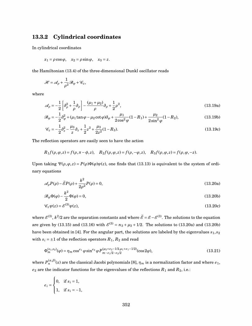
13.3.2 Cylindrical coordinates
In cylindrical coordinates
x1 = ρ cosϕ, x2 = ρ sinϕ, x3 = z.
the Hamiltonian (13.4) of the three-dimensional Dunkl oscillator reads
H =Aρ+ 1ρ2 Bϕ+Cz,
where
Aρ =−12
[∂2ρ+
1ρ∂ρ
]− (µ1 +µ2)
ρ∂ρ+ 1
2ρ2, (13.19a)
Bϕ =−12∂2ϕ+ (µ1 tanϕ−µ2 cotϕ)∂ϕ+ µ1
2cos2ϕ(1−R1)+ µ2
2sin2ϕ(1−R2), (13.19b)
Cz =−12∂2
z −µ3
z∂z + 1
2z2 + µ3
2z2 (1−R3). (13.19c)
The reflection operators are easily seen to have the action
R1 f (ρ,ϕ, z)= f (ρ,π−φ, z), R2 f (ρ,ϕ, z)= f (ρ,−ϕ, z), R3 f (ρ,ϕ, z)= f (ρ,ϕ,−z).
Upon taking Ψ(ρ,ϕ, z) = P(ρ)Φ(ϕ)ψ(z), one finds that (13.13) is equivalent to the system of ordi-
nary equations
AρP(ρ)− E P(ρ)+ k2
2ρ2 P(ρ)= 0, (13.20a)
BϕΦ(ϕ)− k2
2Φ(ϕ)= 0, (13.20b)
Czψ(z)= E (3)ψ(z), (13.20c)
where E (3), k2/2 are the separation constants and where E = E −E (3). The solutions to the equation
are given by (13.15) and (13.16) with E (3) = n3 +µ3 +1/2. The solutions to (13.20a) and (13.20b)
have been obtained in [4]. For the angular part, the solutions are labeled by the eigenvalues s1, s2
with si =±1 of the reflection operators R1, R2 and read
Φ(s1,s2)m (ϕ)= ηm cose1 ϕsine2 ϕP(µ2+e2−1/2,µ1+e1−1/2)
m−e1/2−e2/2 (cos2ϕ), (13.21)
where P(α,β)n (x) are the classical Jacobi polynomials [8], ηm is a normalization factor and where e1,
e2 are the indicator functions for the eigenvalues of the reflections R1 and R2, i.e.:
e i =
0, if si = 1,
1, if si =−1,
352

for i = 1,2. When s1s2 = −1, m is a positive half-integer whereas when s1s2 = 1, m is a non-
negative integer; note also that for m = 0, only the s1 = s2 = 1 state exists. In all parity cases, the
separation constant takes the value
k2 = 4m(m+µ1 +µ2).
If one takes
ηm =[
(2m+µ1 +µ2)Γ(m+µ1 +µ2 + e12 + e2
2 )(m− e12 − e2
2 )!
2Γ(m+µ1 + e12 − e2
2 +1/2)Γ(m+µ2 + e22 − e1
2 +1/2)
]1/2
,
as the normalization factor, the angular part of the separated wavefunction satisfy the orthogo-
nality relation∫ 2π
0Φ
(s1,s2)m Φ
(s′1,s′2)m′ |cosφ|2µ1 |sinφ|2µ2 dφ= δm,m′δs1,s′1δs2,s′2 ,
which can be deduced from the orthogonality relation satisfied by the Jacobi polynomials [8]. The
radial solutions have the expression
Pnρ(ρ)=
[ 2nρ!Γ(nρ+2m+µ1 +µ2 +1)
]1/2
e−ρ2/2ρ2mL(2m+µ1+µ2)
nρ(ρ2), (13.22)
where nρ is a non-negative integer and where L(α)n (x) are the Laguerre polynomials. They satisfy
the orthogonality relation∫ ∞
0Pnρ
(ρ)Pn′ρ(ρ)ρ2µ1+2µ2+1 dρ = δnρ ,n′
ρ.
The separated wavefunctions of the three-dimensional Dunkl oscillator in cylindrical coordinates
are thus given by
Ψnρ ,m,nz (ρ,ϕ, z)= Pnρ(ρ)Φ(s1,s2)
m (ϕ)ψnz (z)
where Pnρ(ρ), Φ(s1,s2)
m (ϕ) and ψnz (z) are given by (13.22), (13.21) and (13.15), respectively. The
energy E is expressed as
E = 2nρ+2m+nz +µ1 +µ2 +µ3 +3/2,
where nρ, nz are non-negative integers and where m is a non-negative integer when s1s2 = 1
or a positive half-integer when s1s2 = −1. In the cylindrical basis, the operators Cz and Bφ are
diagonal with eigenvalues E (3) and k2/2. A direct computation shows that one has
J23 = 2Bϕ+2µ1µ2(1−R1R2),
where J3 is the symmetry given in (13.8). It thus follows that J3 and H3 are the symmetries
responsible for the separation of variables in cylindrical coordinates.
353
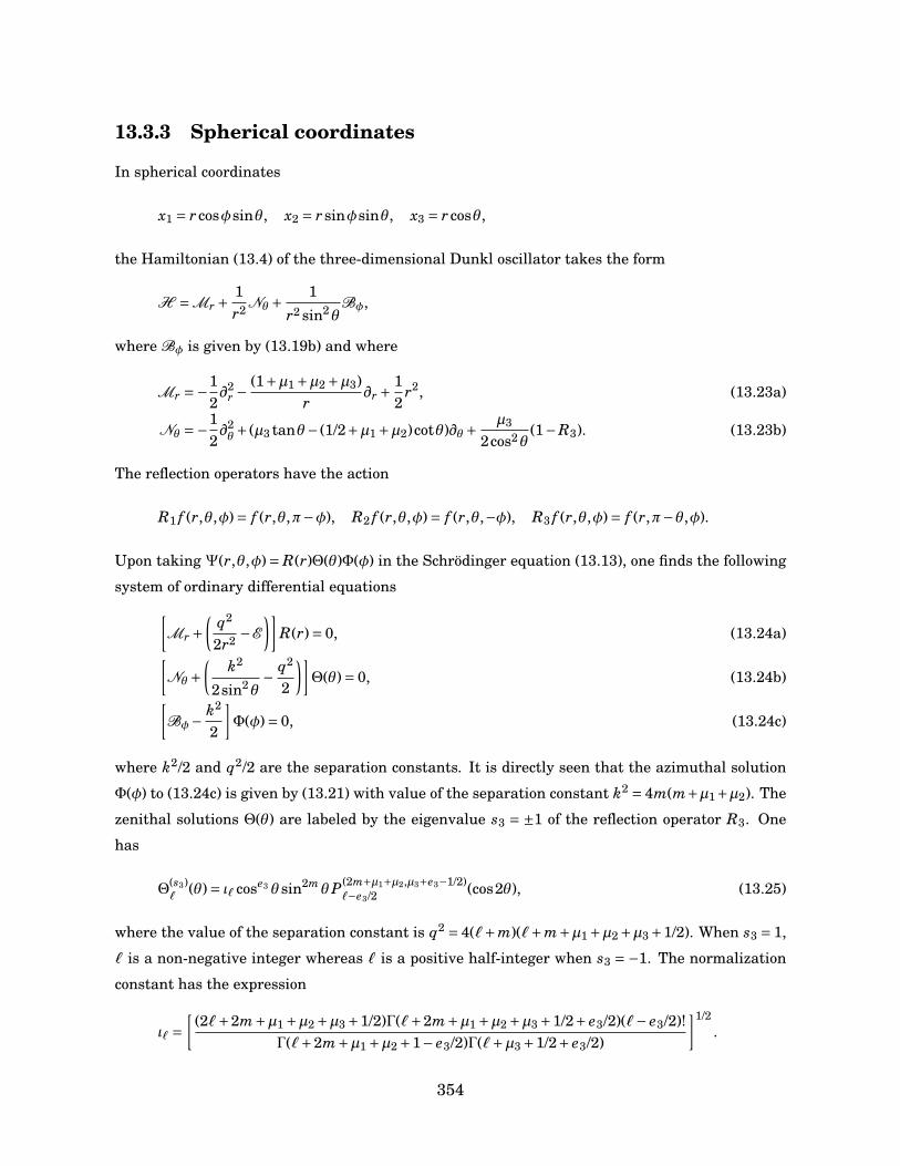
13.3.3 Spherical coordinates
In spherical coordinates
x1 = r cosφsinθ, x2 = rsinφsinθ, x3 = r cosθ,
the Hamiltonian (13.4) of the three-dimensional Dunkl oscillator takes the form
H =Mr + 1r2 Nθ+ 1
r2 sin2θBφ,
where Bφ is given by (13.19b) and where
Mr =−12∂2
r −(1+µ1 +µ2 +µ3)
r∂r + 1
2r2, (13.23a)
Nθ =−12∂2θ+ (µ3 tanθ− (1/2+µ1 +µ2)cotθ)∂θ+ µ3
2cos2θ(1−R3). (13.23b)
The reflection operators have the action
R1 f (r,θ,φ)= f (r,θ,π−φ), R2 f (r,θ,φ)= f (r,θ,−φ), R3 f (r,θ,φ)= f (r,π−θ,φ).
Upon taking Ψ(r,θ,φ)= R(r)Θ(θ)Φ(φ) in the Schrödinger equation (13.13), one finds the following
system of ordinary differential equations[Mr +
(q2
2r2 −E
)]R(r)= 0, (13.24a)[
Nθ+(
k2
2sin2θ− q2
2
)]Θ(θ)= 0, (13.24b)[
Bφ− k2
2
]Φ(φ)= 0, (13.24c)
where k2/2 and q2/2 are the separation constants. It is directly seen that the azimuthal solution
Φ(φ) to (13.24c) is given by (13.21) with value of the separation constant k2 = 4m(m+µ1+µ2). The
zenithal solutions Θ(θ) are labeled by the eigenvalue s3 = ±1 of the reflection operator R3. One
has
Θ(s3)`
(θ)= ι` cose3 θsin2m θP(2m+µ1+µ2,µ3+e3−1/2)`−e3/2 (cos2θ), (13.25)
where the value of the separation constant is q2 = 4(`+m)(`+m+µ1+µ2+µ3+1/2). When s3 = 1,
` is a non-negative integer whereas ` is a positive half-integer when s3 = −1. The normalization
constant has the expression
ι` =[
(2`+2m+µ1 +µ2 +µ3 +1/2)Γ(`+2m+µ1 +µ2 +µ3 +1/2+ e3/2)(`− e3/2)!Γ(`+2m+µ1 +µ2 +1− e3/2)Γ(`+µ3 +1/2+ e3/2)
]1/2.
354
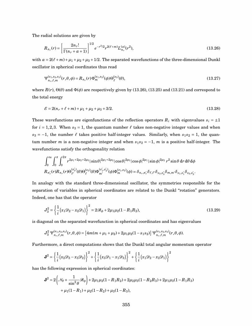
The radial solutions are given by
Rnr (r)=[
2nr!Γ(nr +α+1)
]1/2e−r2/2r2(`+m)L(α)
nr(r2), (13.26)
with α= 2(`+m)+µ1+µ2+µ3+1/2. The separated wavefunctions of the three-dimensional Dunkl
oscillator in spherical coordinates thus read
Ψ(s1,s2,s3)nr ,`,m (r,θ,φ)= Rnr (r)Φ(s1,s2)
m (φ)Θ(s3)`
(θ), (13.27)
where R(r), Θ(θ) and Φ(φ) are respectively given by (13.26), (13.25) and (13.21) and correspond to
the total energy
E = 2(nr +`+m)+µ1 +µ2 +µ3 +3/2. (13.28)
These wavefunctions are eigenfunctions of the reflection operators Ri with eigenvalues si = ±1
for i = 1,2,3. When s3 = 1, the quantum number ` takes non-negative integer values and when
s3 = −1, the number ` takes positive half-integer values. Similarly, when s1s2 = 1, the quan-
tum number m is a non-negative integer and when s1s2 = −1, m is a positive half-integer. The
wavefunctions satisfy the orthogonality relation∫ ∞
0
∫ π
0
∫ 2π
0r2µ1+2µ2+2µ3 |sinθ|2µ1+2µ2 |cosθ|2µ3 |cosφ|2µ1 |sinφ|2µ2 r2 sinθ drdθdφ
Rn′r(r)Rnr (r)Θ(s′3)
`′ (θ)Θ(s3)`
(θ)Φ(s′1,s′2)m′ (φ)Φ(s1,s2)
m (φ)= δnr ,n′rδ`,`′δs3,s′3δm,m′δs1,s′1δs2,s′2 .
In analogy with the standard three-dimensional oscillator, the symmetries responsible for the
separation of variables in spherical coordinates are related to the Dunkl “rotation” generators.
Indeed, one has that the operator
J23 =
1i(x1D2 − x2D1
)2= 2Bφ+2µ1µ2(1−R1R2), (13.29)
is diagonal on the separated wavefunction in spherical coordinates and has eigenvalues
J23 Ψ
(s1,s2,s3)nr ,`,m (r,θ,φ)= [
4m(m+µ1 +µ2)+2µ1µ2(1− s1s2)]Ψ
(s1,s2,s3)nr ,`,m (r,θ,φ).
Furthermore, a direct computations shows that the Dunkl total angular momentum operator
J2 =
1i(x2D3 − x3D2
)2+
1i(x3D1 − x1D3
)2+
1i(x1D2 − x2D1
)2
has the following expression in spherical coordinates:
J2 = 2(Nθ+ 1
sin2θBφ
)+2µ1µ2(1−R1R2)+2µ2µ3(1−R2R3)+2µ1µ3(1−R1R3)
+µ1(1−R1)+µ2(1−R2)+µ3(1−R3),
355
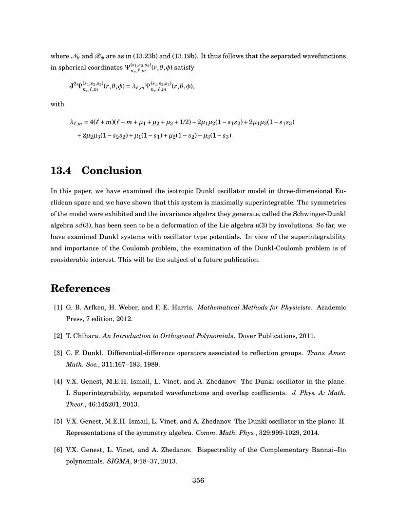
where Nθ and Bφ are as in (13.23b) and (13.19b). It thus follows that the separated wavefunctions
in spherical coordinates Ψ(s1,s2,s3)nr ,`,m (r,θ,φ) satisfy
J2Ψ(s1,s2,s3)nr ,`,m (r,θ,φ)=λ`,mΨ
(s1,s2,s3)nr ,`,m (r,θ,φ),
with
λ`,m = 4(`+m)(`+m+µ1 +µ2 +µ3 +1/2)+2µ1µ2(1− s1s2)+2µ1µ3(1− s1s3)
+2µ2µ3(1− s2s2)+µ1(1− s1)+µ2(1− s2)+µ3(1− s3).
13.4 Conclusion
In this paper, we have examined the isotropic Dunkl oscillator model in three-dimensional Eu-
clidean space and we have shown that this system is maximally superintegrable. The symmetries
of the model were exhibited and the invariance algebra they generate, called the Schwinger-Dunkl
algebra sd(3), has been seen to be a deformation of the Lie algebra u(3) by involutions. So far, we
have examined Dunkl systems with oscillator type potentials. In view of the superintegrability
and importance of the Coulomb problem, the examination of the Dunkl-Coulomb problem is of
considerable interest. This will be the subject of a future publication.
References[1] G. B. Arfken, H. Weber, and F. E. Harris. Mathematical Methods for Physicists. Academic
Press, 7 edition, 2012.
[2] T. Chihara. An Introduction to Orthogonal Polynomials. Dover Publications, 2011.
[3] C. F. Dunkl. Differential-difference operators associated to reflection groups. Trans. Amer.
Math. Soc., 311:167–183, 1989.
[4] V.X. Genest, M.E.H. Ismail, L. Vinet, and A. Zhedanov. The Dunkl oscillator in the plane:
I. Superintegrability, separated wavefunctions and overlap coefficients. J. Phys. A: Math.
Theor., 46:145201, 2013.
[5] V.X. Genest, M.E.H. Ismail, L. Vinet, and A. Zhedanov. The Dunkl oscillator in the plane: II.
Representations of the symmetry algebra. Comm. Math. Phys., 329:999-1029, 2014.
[6] V.X. Genest, L. Vinet, and A. Zhedanov. Bispectrality of the Complementary Bannai–Ito
polynomials. SIGMA, 9:18–37, 2013.
356
[7] V.X. Genest, L. Vinet, and A. Zhedanov. The singular and 2:1 anisotropic Dunkl oscillators in
the plane. J. Phys. A: Math. Theor., 46:325201, 2013.
[8] R. Koekoek, P.A. Lesky, and R.F. Swarttouw. Hypergeometric orthogonal polynomials and
their q-analogues. Springer, 1st edition, 2010.
[9] W. Miller, S. Post, and P. Winternitz. Classical and quantum superintegrability with applica-
tions. J. Phys. A: Math. Theor., 46:423001, 2013.
[10] N. Mukunda, E. C. G. Sudarshan, J. K. Sharma, and C. L. Mehta. Representations and
properties of para-Bose oscillator operators I. Energy position and momentum eigenstates. J.
Math. Phys., 21:2386, 1980.
[11] S. Tsujimoto, L. Vinet, and A. Zhedanov. From slq(2) to a parabosonic Hopf algebra. SIGMA,
7:93–105, 2011.
[12] S. Tsujimoto, L. Vinet, and A. Zhedanov. Dunkl shift operators and Bannai–Ito polynomials.
Adv. Math., 229:2123–2158, 2012.
357

358
Chapitre 14
The Bannai–Ito algebra and asuperintegrable system withreflections on the 2-sphere
V. X. Genest, L. Vinet et A. Zhedanov (2014). The Bannai–Ito algebra and a superintegrable
system with reflections on the 2-sphere. Journal of Physics A: Mathematical and Theoretical 47
205202
Abstract. A quantum superintegrable model with reflections on the 2-sphere is introduced. Its
two algebraically independent constants of motion generate a central extension of the Bannai–Ito
algebra. The Schrödinger equation separates in spherical coordinates and its exact solutions are
presented. It is further observed that the Hamiltonian of the system arises in the addition of three
representations of the sl−1(2) algebra (the dynamical algebra of the one-dimensional parabosonic
oscillator). The contraction from the two-sphere to the Euclidean plane yields the Dunkl oscillator
in two dimensions and its Schwinger-Dunkl symmetry algebra sd(2).
14.1 Introduction
The class of superintegrable quantum systems is of particular interest as a laboratory for the
study of symmetries, their algebraic description and their representations. A quantum system in
n dimensions with Hamiltonian H is said to be maximally superintegrable if it possesses 2n−1
algebraically independent constants of motion ci for i = 1, . . . ,2n−1 commuting with H, [H, ci]= 0,
where one of these constants is H. A system is of order ` if the maximum order in momenta of
the constants of motion (other than H) is `. Empirically, superintegrable systems turn out to be
359
exactly solvable.
The category of models that has been most analyzed is that of systems governed by scalar
Hamiltonians of the form
H =∆+V , (14.1a)
where ∆ is the standard Laplacian
∆= 1√det g
∂
∂xi
√det g gi j ∂
∂x j, (14.1b)
on spaces with metric g i j in coordinates xi. In two dimensions, the second order superintegrable
models of that type have been identified and classified [25]. As a matter of fact, they can all
be obtained from the generic 3-parameter model on the two-sphere by limits (contractions) and
specializations (see [20] for details). By observing that the Hamiltonian of the generic model on
the two-sphere can be constructed through the addition of three su(1,1) algebras, the constants
of motion were identified in [9, 14] as the intermediate Casimir operators arising in the step-
wise combination process. These were further shown to generate the Racah algebra which is the
quadratic algebra with two independent generators that captures the bispectrality of the Racah
polynomials sitting atop the discrete side of the Askey tableau of hypergeometric polynomials [22].
This identification of the symmetry algebra hence allows to associate the Racah polynomials to the
generic 3-parameter superintegrable system on the 2-sphere. A threefold connection between the
polynomials of the Askey scheme, the second-order superintegrable models and their symmetry
algebras can further be achieved by performing on the Racah polynomials and the Racah algebras
the contractions and specializations that lead from the generic model on the two-sphere to the
other second-order superintegrable systems [20].
The exploration of another category of superintegrable models has been undertaken recently:
it bears on systems whose Hamiltonians involve reflections. Typically, the involutions arise in
Dunkl operators [4] which are defined as follows in the special univariate case:
Dµx = ∂x + µ
x(1−Rx), (14.2)
where ∂x stands for the derivative with respect to x and where Rx is the reflection operator such
that Rx f (x)= f (−x). One of the simplest dynamical systems with reflections is the parabose oscil-
lator in one dimension with Hamiltonian (see [26])
H = (Dµx)2 + x2.
Other one-dimensional models have been discussed (see for example [18, 21, 28]). Recall that
Dunkl operators are most useful in the study of multivariate orthogonal polynomials associated
360
to reflection groups [5] and that of symmetric functions [24] as well as in the analysis of exactly
solvable quantum many-body systems of Calogero-Sutherland type (see for instance [23]).
Interestingly, the theory of univariate orthogonal polynomials that are eigenfunctions of dif-
ferential or difference operators of Dunkl type has also been the object of attention lately [10, 13,
31, 32, 33, 34, 35]. These are now referred to as −1 polynomials and a scheme similar to the Askey
one has emerged for them. Taking a place analogous to that of the Racah polynomials are the
Bannai–Ito polynomials, which are sitting at the top of one side of the −1 tableau and which were
introduced in a combinatorial context [3]. The characteristic properties of these polynomials are
encoded [7, 16, 31] in an algebra bearing the Bannai–Ito name which has 3 generators L1, L2 and
L3 verifying the following relations given in terms of anticommutators (A,B= AB+BA):
L1,L2= L3 +ω3, L2,L3= L1 +ω1, L3,L1= L2 +ω2, (14.3)
where ω1, ω2, ω3 are central. Introduced in [31], the algebra (14.3) is the structure behind the
bispectrality property of the Bannai–Ito polynomials. It corresponds to a q →−1 limit of the Askey-
Wilson algebra [36], which is the algebra behind the bispectrality property of the q-polynomials of
the Askey scheme [22]; it has also been used in [30] to study structure relations for −1 polynomials
of the Bannai–Ito family. The special case with ω1 =ω2 =ω3 = 0 has been studied in [2, 17] as an
anticommutator version of the Lie algebra su(2).
The examination of superintegrable systems with reflections has mostly focused so far on
Dunkl oscillators in the plane [11, 12, 15] and in R3 [8]. These are formed out of combinations
of one-dimensional parabose systems (with the inclusions of possible singular terms). They all are
superintegrable and exactly solvable. In the “isotropic” case, the symmetry algebra denoted sd(n)
is a deformation of su(n) with n the number of dimensions. The Dunkl oscillators have proved to
be showcases for −1 polynomials. An infinite family of higher order (`> 2) superintegrable models
with reflections has also been obtained with the help of the little −1 Jacobi polynomials [27].
The purpose of this paper is to introduce and analyze an elegant superintegrable model with
reflections on the two-sphere. The symmetry algebra will be seen to be a central extension of the
Bannai–Ito algebra, a first physical occurrence as such of this algebra, as far as we know. This
model-algebra pairing will present itself as the analog in the presence of reflections of the teaming
of the Racah algebra with the so-called generic 3-parameter system on the two-sphere. It entails
a relation [7] between Dunkl harmonic analysis on the 2-sphere and the representation theory of
sl−1(2), a q →−1 limit of the quantum algebra Uq(sl2) that can be identified with the dynamical
algebra of the parabose oscillator [29].
The outline of the paper is as follows. In Section 2, the model is described, the constants of
motion are exhibited and the invariance algebra they generate is identified as a central extension
of the Bannai–Ito algebra. In section 3, the separated solutions of the model are given explicitly
361
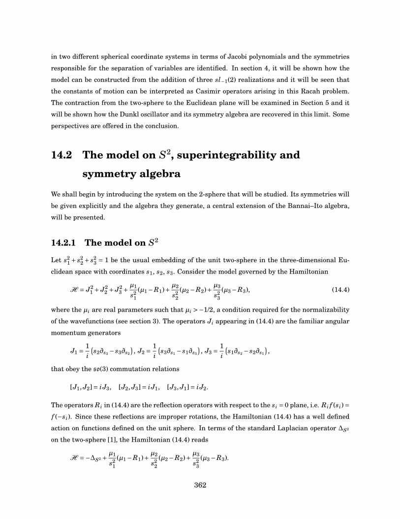
in two different spherical coordinate systems in terms of Jacobi polynomials and the symmetries
responsible for the separation of variables are identified. In section 4, it will be shown how the
model can be constructed from the addition of three sl−1(2) realizations and it will be seen that
the constants of motion can be interpreted as Casimir operators arising in this Racah problem.
The contraction from the two-sphere to the Euclidean plane will be examined in Section 5 and it
will be shown how the Dunkl oscillator and its symmetry algebra are recovered in this limit. Some
perspectives are offered in the conclusion.
14.2 The model on S2, superintegrability and
symmetry algebra
We shall begin by introducing the system on the 2-sphere that will be studied. Its symmetries will
be given explicitly and the algebra they generate, a central extension of the Bannai–Ito algebra,
will be presented.
14.2.1 The model on S2
Let s21 + s2
2 + s23 = 1 be the usual embedding of the unit two-sphere in the three-dimensional Eu-
clidean space with coordinates s1, s2, s3. Consider the model governed by the Hamiltonian
H = J21 + J2
2 + J23 + µ1
s21
(µ1 −R1)+ µ2
s22
(µ2 −R2)+ µ3
s23
(µ3 −R3), (14.4)
where the µi are real parameters such that µi >−1/2, a condition required for the normalizability
of the wavefunctions (see section 3). The operators Ji appearing in (14.4) are the familiar angular
momentum generators
J1 = 1i(s2∂s3 − s3∂s2
), J2 = 1
i(s3∂s1 − s1∂s3
), J3 = 1
i(s1∂s2 − s2∂s1
),
that obey the so(3) commutation relations
[J1, J2]= iJ3, [J2, J3]= iJ1, [J3, J1]= iJ2.
The operators Ri in (14.4) are the reflection operators with respect to the si = 0 plane, i.e. Ri f (si)=f (−si). Since these reflections are improper rotations, the Hamiltonian (14.4) has a well defined
action on functions defined on the unit sphere. In terms of the standard Laplacian operator ∆S2
on the two-sphere [1], the Hamiltonian (14.4) reads
H =−∆S2 + µ1
s21
(µ1 −R1)+ µ2
s22
(µ2 −R2)+ µ3
s23
(µ3 −R3).
362
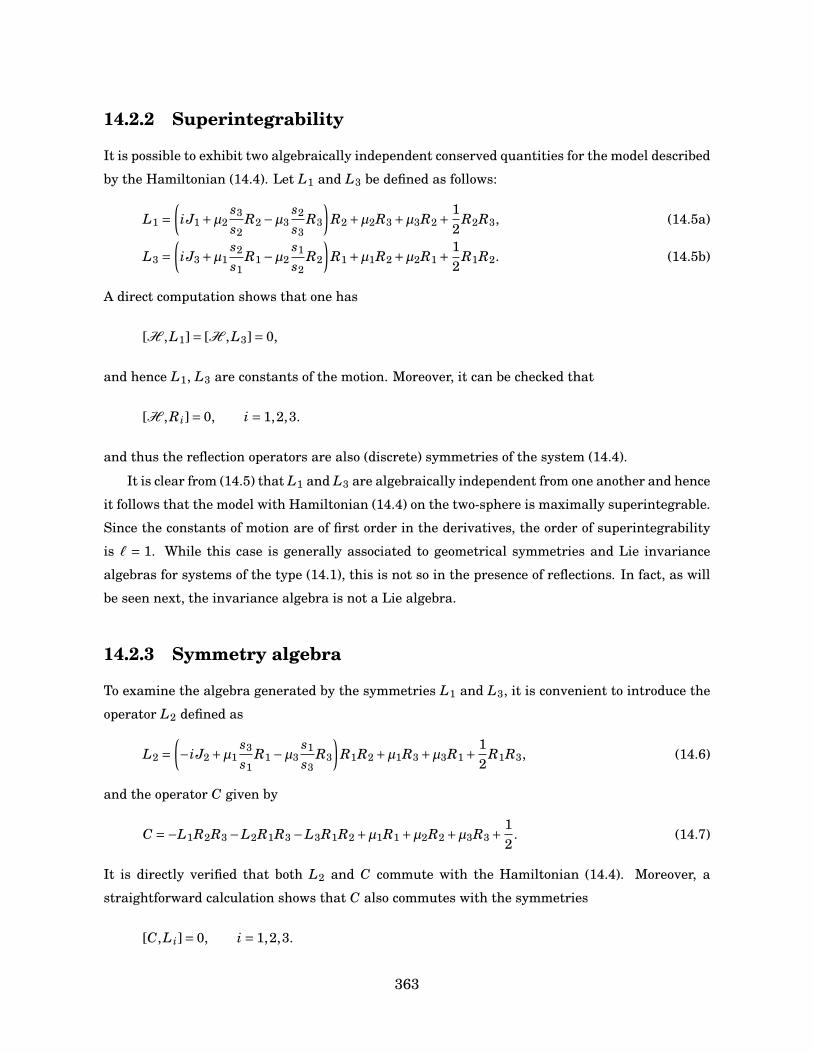
14.2.2 Superintegrability
It is possible to exhibit two algebraically independent conserved quantities for the model described
by the Hamiltonian (14.4). Let L1 and L3 be defined as follows:
L1 =(iJ1 +µ2
s3
s2R2 −µ3
s2
s3R3
)R2 +µ2R3 +µ3R2 + 1
2R2R3, (14.5a)
L3 =(iJ3 +µ1
s2
s1R1 −µ2
s1
s2R2
)R1 +µ1R2 +µ2R1 + 1
2R1R2. (14.5b)
A direct computation shows that one has
[H ,L1]= [H ,L3]= 0,
and hence L1, L3 are constants of the motion. Moreover, it can be checked that
[H ,Ri]= 0, i = 1,2,3.
and thus the reflection operators are also (discrete) symmetries of the system (14.4).
It is clear from (14.5) that L1 and L3 are algebraically independent from one another and hence
it follows that the model with Hamiltonian (14.4) on the two-sphere is maximally superintegrable.
Since the constants of motion are of first order in the derivatives, the order of superintegrability
is ` = 1. While this case is generally associated to geometrical symmetries and Lie invariance
algebras for systems of the type (14.1), this is not so in the presence of reflections. In fact, as will
be seen next, the invariance algebra is not a Lie algebra.
14.2.3 Symmetry algebra
To examine the algebra generated by the symmetries L1 and L3, it is convenient to introduce the
operator L2 defined as
L2 =(−iJ2 +µ1
s3
s1R1 −µ3
s1
s3R3
)R1R2 +µ1R3 +µ3R1 + 1
2R1R3, (14.6)
and the operator C given by
C =−L1R2R3 −L2R1R3 −L3R1R2 +µ1R1 +µ2R2 +µ3R3 + 12
. (14.7)
It is directly verified that both L2 and C commute with the Hamiltonian (14.4). Moreover, a
straightforward calculation shows that C also commutes with the symmetries
[C,L i]= 0, i = 1,2,3.
363
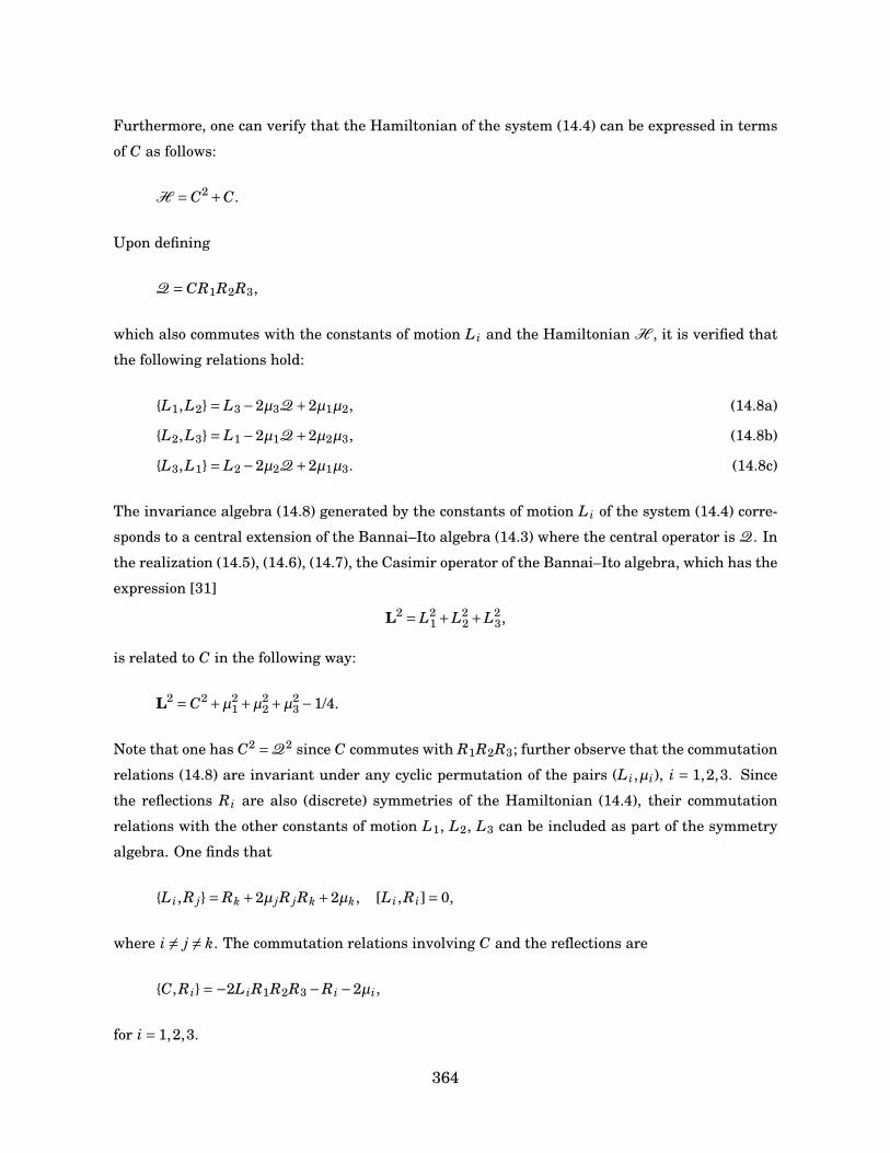
Furthermore, one can verify that the Hamiltonian of the system (14.4) can be expressed in terms
of C as follows:
H = C2 +C.
Upon defining
Q = CR1R2R3,
which also commutes with the constants of motion L i and the Hamiltonian H , it is verified that
the following relations hold:
L1,L2= L3 −2µ3Q+2µ1µ2, (14.8a)
L2,L3= L1 −2µ1Q+2µ2µ3, (14.8b)
L3,L1= L2 −2µ2Q+2µ1µ3. (14.8c)
The invariance algebra (14.8) generated by the constants of motion L i of the system (14.4) corre-
sponds to a central extension of the Bannai–Ito algebra (14.3) where the central operator is Q. In
the realization (14.5), (14.6), (14.7), the Casimir operator of the Bannai–Ito algebra, which has the
expression [31]
L2 = L21 +L2
2 +L23,
is related to C in the following way:
L2 = C2 +µ21 +µ2
2 +µ23 −1/4.
Note that one has C2 =Q2 since C commutes with R1R2R3; further observe that the commutation
relations (14.8) are invariant under any cyclic permutation of the pairs (L i,µi), i = 1,2,3. Since
the reflections Ri are also (discrete) symmetries of the Hamiltonian (14.4), their commutation
relations with the other constants of motion L1, L2, L3 can be included as part of the symmetry
algebra. One finds that
L i,R j= Rk +2µ jR jRk +2µk, [L i,Ri]= 0,
where i 6= j 6= k. The commutation relations involving C and the reflections are
C,Ri=−2L iR1R2R3 −Ri −2µi,
for i = 1,2,3.
364
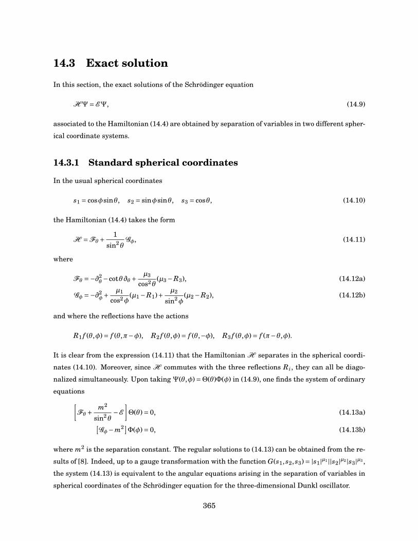
14.3 Exact solution
In this section, the exact solutions of the Schrödinger equation
HΨ= EΨ, (14.9)
associated to the Hamiltonian (14.4) are obtained by separation of variables in two different spher-
ical coordinate systems.
14.3.1 Standard spherical coordinates
In the usual spherical coordinates
s1 = cosφsinθ, s2 = sinφsinθ, s3 = cosθ, (14.10)
the Hamiltonian (14.4) takes the form
H =Fθ+ 1sin2θ
Gφ, (14.11)
where
Fθ =−∂2θ−cotθ∂θ+ µ3
cos2θ(µ3 −R3), (14.12a)
Gφ =−∂2φ+
µ1
cos2φ(µ1 −R1)+ µ2
sin2φ(µ2 −R2), (14.12b)
and where the reflections have the actions
R1 f (θ,φ)= f (θ,π−φ), R2 f (θ,φ)= f (θ,−φ), R3 f (θ,φ)= f (π−θ,φ).
It is clear from the expression (14.11) that the Hamiltonian H separates in the spherical coordi-
nates (14.10). Moreover, since H commutes with the three reflections Ri, they can all be diago-
nalized simultaneously. Upon taking Ψ(θ,φ)=Θ(θ)Φ(φ) in (14.9), one finds the system of ordinary
equations[Fθ+ m2
sin2θ−E
]Θ(θ)= 0, (14.13a)[
Gφ−m2]Φ(φ)= 0, (14.13b)
where m2 is the separation constant. The regular solutions to (14.13) can be obtained from the re-
sults of [8]. Indeed, up to a gauge transformation with the function G(s1, s2, s3)= |s1|µ1 ||s2|µ2 |s3|µ3 ,
the system (14.13) is equivalent to the angular equations arising in the separation of variables in
spherical coordinates of the Schrödinger equation for the three-dimensional Dunkl oscillator.
365
Using this observation and the results of [8], one finds that the azimuthal solutions have the
following expression:
Φ(e1,e2)n (φ)=
((n+µ1 +µ2)
( n−e1−e22
)!Γ( n+e1+e2
2 +µ1 +µ2)
2Γ( n+e1−e22 +µ1 +1/2)Γ( n+e2−e1
2 +µ2 +1/2)
)1/2
|cosφ|µ1 |sinφ|µ2 cose1 φsine2 φ P(µ2−1/2+e2,µ1−1/2+e1)(n−e1−e2)/2 (cos2φ), (14.14)
where P(α,β)n (x) are the Jacobi polynomials [22], Γ(z) is the Gamma function [1] and where e i ∈
0,1. The azimuthal solutions (14.14) satisfy the eigenvalue equations
R1Φ(e1,e2)n (φ)= (1−2e1)Φ(e1,e2)
n (φ), R2Φ(e1,e2)n (φ)= (1−2e2)Φ(e1,e2)
n (φ),
with respect to the reflections. They obey the orthogonality relation∫ 2π
0Φ
(e1,e2)n (φ)Φ(e′1,e′2)
n′ (φ) dφ= δnn′δe1e′1δe2e′2 ,
as can be checked by comparing with the orthogonality relation satisfied by the Jacobi polynomials
[22]. The separation constant here takes the value m2 = (n+µ1 +µ2)2. When e1 + e2 = 1, n is a
positive odd integer, when e1+ e2 = 0, n is a non-negative even integer and when e1+ e2 = 2, n is a
positive even integer. The regular solutions to the zenithal equation (14.13a) are of the form [8]
Θ(e3)n;N (θ)=
((N +µ1 +µ2 +µ3 +1/2)( N−n−e3
2 )!Γ( N+n+e32 +µ1 +µ2 +µ3 +1/2)
Γ( N+n−e32 +µ1 +µ2 +1)Γ( N−n+e3
2 +µ3 +1/2)
)1/2
|sinθ|µ1+µ2 |cosθ|µ3 sinn θ cose3 θ P(n+µ1+µ2,µ3−1/2+e3)(N−n−e3)/2 (cos2θ). (14.15)
with e3 ∈ 0,1. The following eigenvalue equation holds:
R3Θ(e3)n;N (θ)= (1−2e3)Θ(e3)
n;N (θ).
The energy E corresponding to the solution (14.15) is given by
EN = (N +µ1 +µ2 +µ3)2 + (N +µ1 +µ2 +µ3), (14.16)
where N is a non-negative integer. The complete wavefunctions of the Hamiltonian (14.4) on the
2-sphere with energy EN given by (14.16) thus have the expression
Ψ(e1,e2,e3)n;N (θ,φ)=Θ(e3)
n;N (θ)Φ(e1,e2)n (φ),
where the zenithal and azimuthal parts are given by (14.15) and (14.14), respectively. By a direct
counting of the admissible states (taking into account the fact that values of the quantum numbers
N, n, e i yielding half-integer or negative values of k in the Jacobi polynomials P(α,β)k (x) are not
366
admissible), it is seen that the EN energy eigenspace is (2N+1)-fold degenerate. Furthermore, one
observes that
R1R2R3Ψ(e1,e2,e3)n;N (θ,φ)= (−1)NΨ
(e1,e2,e3)n;N (θ,φ),
and that the wavefunctions satisfy the orthogonality relation∫ π
0
∫ 2π
0Ψ
(e1,e2,e3)n;N (θ,φ)Ψ(e′1,e′2,e′3)
n′;N ′ (θ,φ) sinθdφdθ = δnn′δNN ′δe1e′1δe2e′2δe3e′3 .
The symmetry operator responsible for the separation of variables in spherical coordinates is L3.
Indeed, a direct computation shows that upon defining Z = L3R1R2 one has
Z2 −Z+ 14=Gφ,
where Gφ is given by (14.12b).
14.3.2 Alternative spherical coordinates
The Schrödinger equation (14.9) associated to the Hamiltonian on the 2-sphere (14.4) also sepa-
rates in the alternative spherical coordinate system where the coordinates s1, s2, s3 of the 2-sphere
are parametrized as follows:
s1 = cosϑ, s2 = cosϕsinϑ, s3 = sinϕsinϑ. (14.17)
In these coordinates the Hamiltonian (14.4) takes the from
H = Fϑ+ 1sin2ϑ
Gϕ,
where
Fϑ =−∂2ϑ−cotϑ∂ϑ+ µ1
cos2ϑ(µ1 −R1), (14.18a)
Gϕ =−∂2ϕ+
µ2
cos2ϕ(µ2 −R2)+ µ3
sin2ϕ(µ3 −R3), (14.18b)
and where the reflections have the actions
R1 f (ϑ,ϕ)= f (π−ϑ,ϕ), R2 f (ϑ,ϕ)= f (ϑ,π−ϕ), R3 f (ϑ,ϕ)= f (ϑ,−ϕ). (14.19)
Upon comparing (14.18) with (14.12) it is clear that the solutions to the Schrödinger equation
(14.9) in the alternative coordinate system (14.17) have the expression
Ψ(e1,e2,e3)n;N (ϑ,ϕ)=πΘ(e1)
n;N (ϑ)Φ(e2,e3)n (ϕ),
367
where π = (123) indicates the permutation applied to the parameters (µ1,µ2,µ3). The symmetry
associated to the separation of variables in the alternative coordinate system (14.17) is L1 since
upon taking Y = L1R2R3, one finds that
Y 2 −Y + 14= Gϕ.
As illustrated above, the origin of the two independent constants of motion L3 and L1 of the model
(14.4) on the two-sphere can be traced back to the multiseparability of the Schrödinger equation
in the usual and alternative spherical coordinates, respectively. This situation is analogous to the
one arising in the analysis of the generic three-parameter system on the 2-sphere (without reflec-
tions) for which the symmetries generating the Racah algebra are associated to the separation
of variables in different spherical coordinate systems [9]. In this case, the expansion coefficients
coefficients between the separated wavefunctions in the coordinate systems (14.10) and (14.17)
coincide with the 6 j symbols of su(1,1).
14.4 Connection with sl−1(2)
In this section, it is shown how of the Hamiltonian (14.4) of the model on the 2-sphere arises in
the combination of three realizations of the sl−1(2) algebra, which we loosely refer to as the Racah
problem for sl−1(2).
14.4.1 sl−1(2) algebra
The sl−1(2) algebra was introduced in [29] as a q →−1 limit of the quantum algebra Uq(sl2). It
has three three generators A±, A0 and one involution P and is defined by the relations
[A0, A±]=±A±, [A0,P]= 0, A+, A−= 2A0, A±,P= 0, P2 = 1. (14.20)
The Casimir operator of sl−1(2), which commutes with all generators, is given by
Q = A+A−P − A0P +P/2.
Let A(i)0 , A(i)
± and P(i), i = 1,2,3, denote three mutually commuting sets of sl−1(2) generators.
Using the coproduct of sl−1(2) (see [29]), the three sets can be combined to produce a fourth set of
generators satisfying the relations (14.20). The elements of this fourth set A0,A±,P are defined
by
A0 = A(1)0 + A(2)
0 + A(3)0 , (14.21a)
A± = A(1)± P(2)P(3) + A(2)
± P(3) + A(3)± , (14.21b)
P = P(1)P(2)P(3). (14.21c)
368
It is easily verified that the operators (14.21) indeed satisfy the defining relations (14.20) of sl−1(2).
In the combining of these independent sets of sl−1(2) generators, three types of Casimir operators
should be distinguished. The initial Casimir operators Q(i)
Q(i) = A(i)+ A(i)
− P(i) − A(i)0 P(i) +P(i)/2, i = 1,2,3,
which are attached to each independent set of sl−1(2) generators. The two intermediate Casimir
operators Q(i j)
Q(i j) = (A(i)− A( j)
+ − A(i)+ A( j)
− )P(i) +Q(i)P( j) +Q( j)P(i) −P(i)P( j)/2,
for (i j) = (12), (23) which are associated to the step-wise combination process. The total Casimir
operator Q associated to the fourth set
Q =A+A−P −A0P +P /2,
which has the expression
Q = (A(1)− A(3)
+ − A(1)+ A(3)
− )P(1) −Q(2)P(1)P(3) +Q(12)P(3) +Q(23)P(1).
The intermediate Casimir operators commute with both the initial and the total Casimir operators
and with P , but do not commute amongst themselves. As a matter of fact, it was established in
[16] that on representations spaces where the total Casimir operator Q is diagonal, the interme-
diate Casimir operators Q(i j) generate the Bannai–Ito algebra.
14.4.2 Differential/Difference realization and
the model on the 2-sphere
The connection between the combination of three sl−1(2) algebras and the superintegrable sys-
tem on the two-sphere defined by (14.4) can now be established. Consider the following differen-
tial/difference realization of sl−1(2):
A(i)± = 1p
2
[si ∓∂si ±
µi
siRi
], (14.22a)
A(i)0 = 1
2
[−∂2
si+ s2
i +µi
s2i(µi −Ri)
], (14.22b)
P(i) = Ri. (14.22c)
Note that with respect to the uniform measure on the real line, A(i)0 is Hermitian and A(i)
± are
Hermitian conjugates. Up to a gauge transformation of the generators
z →G(si)−1zG(si), z ∈ A(i)± , A(i)
0 ,P(i),
369
with gauge function G(si)= |si|µi , the realization (14.22) is equivalent to the realization of sl−1(2)
arising in the one-dimensional parabose oscillator [11]. Using (14.22), the initial Casimir operators
Q(i) are seen to have the action
Q(i) f (si)=−µi f (si).
and the intermediate Casimir operators take the form
Q(12) =[(s1∂s2 − s2∂s1)+µ1
s2
s1R1 −µ2
s1
s2R2
]R1 +µ1R2 +µ2R1 + 1
2R1R2,
Q(23) =[(s2∂s3 − s3∂s2)+µ2
s3
s2R2 −µ3
s2
s3R3
]R2 +µ2R3 +µ3R2 + 1
2R2R3.
(14.23)
Furthermore, an explicit computation shows that upon defining Ω=QP , one finds
Ω2 +Ω=
J21 + J2
2 + J23 + (s2
1 + s22 + s2
3)
(µ1
s21
(µ1 −R1)+ µ2
s22
(µ2 −R2)+ µ3
s23
(µ3 −R3)
). (14.24)
Upon comparing the expressions (14.23) for the intermediate Casimir operators with the formulas
(14.5) for the constants of motion, it is seen that
Q(12) =−L3, Q(23) =−L1,
and thus that the intermediate Casimir coincide with the constants of motion. Upon comparing
(14.24) with the Hamiltonian (14.4), it is also seen that
Ω2 +Ω=H ,
given the condition s21 + s2
2 + s23 = 1. This condition can be ensured in general. Indeed, one checks
that
X2 = 12
(A++A−)2 = s21 + s2
2 + s23.
Since X2 commutes with Ω and all the intermediate Casimir operators, it is central in the invari-
ance algebra (14.8) and can thus be treated as a constant. Hence one can take X2 = 1 without
loss of generality and complete the identification of the quadratic combination Ω2 +Ω with the
Hamiltonian H .
The analysis of the model on the 2-sphere defined by the Hamiltonian (14.4) is thus related to
the combination of three independent realizations of the sl−1(2) algebra. The constants of motion
of the system correspond to the intermediate Casimir operators arising in this combination and
the Hamiltonian is related to a quadratic combination of the total Casimir operator (times P ).
370
It is worth pointing out that in [9, 14] the Hamiltonian of the three-parameter model on the two-
sphere (without reflections) was directly identified to the total Casimir operator in the combination
of three su(1,1) realizations. Here the total Casimir operator Q (or equivalently Ω) is of first order
in derivatives and hence a quadratic combination must me taken to recover the Hamiltonian
(14.4) of the model. As a remark, let us note that the relation (14.24) is reminiscent of chiral
supersymmetry. Indeed, if one defines a new Hamiltonian by H =H +1/4, then H = 12 Q,Q where
Q =Ω+1/2. In this picture, Q =Ω+1/2 can be interpreted as a chiral supercharge for H. See also
[6] for related considerations.
14.5 Superintegrable model in the plane
from contraction
The results obtained so far are analogous to those of [9, 14] where the analysis of the generic
3-parameter system on the two-sphere was cast in the framework of the Racah problem for the
su(1,1) algebra. Given that the model (14.4) is the analogue with reflections of the generic 3-
parameter system on the 2-sphere and since all second-order superintegrable systems can be
obtained from the latter [20], it is natural to ask whether contractions of (14.4) lead to other
superintegrable systems with reflections. The answer to that question is in the positive. As an
example, we describe in this section how the Dunkl oscillator model in the plane and its con-
served quantities can be obtained from a contraction of the system (14.4) on the two-sphere and
its symmetries.
14.5.1 Contraction of the Hamiltonian
Consider the Hamiltonian
H = J21 + J2
2 + J23 + (s2
1 + s22 + s2
3)
(µ2
1 −µ1R1
s21
+ µ22 −µ2R2
s22
+ µ23 −µ3R3
s23
), (14.25)
which is equivalent to (14.4) in view of the results of section 4. The two-sphere s21 + s2
2 + s33 = r2 of
radius r can be contracted to the Euclidean plane with coordinates x1, x2 by taking the limit as
r →∞ in
x1 = rs1
s3, x2 = r
s2
s3, s2
3 = r2 − s21 − s2
2, (14.26)
371
Changing the variables in (14.25) according to the prescription (14.26) and defining µ3 = µ3r2, a
direct computation shows that
H ≡ limr→∞
1r2
(H −µ2
3 +µ3R3
)=
−∂2x1−∂2
x2+ µ1
x21
(µ1 −R1)+ µ2
x22
(µ2 −R2)+ µ23(x2
1 + x22).
(14.27)
The Hamiltonian H corresponds, up to a gauge transformation, to the Hamiltonian of the Dunkl
oscillator model in the plane. Indeed, taking H →|x1|−µ1 |x2|−µ2H |x2|µ2 |x1|µ1 , one finds that
H →−[(Dµ1
x1 )2 + (Dµ2x2 )2]+ µ2
3(x21 + x2
2), (14.28)
where Dµx is the Dunkl derivative (14.2). Taking µ3 = 1, the Hamiltonian (14.28) coincides with
that of the model examined in [11].
14.5.2 Contraction of the constants of motion
The conserved quantities of the Dunkl oscillator in the plane can be recovered by a contraction of
the symmetry operators of the Hamiltonian (14.25). Since the reflections commute with (14.25),
one can consider the following form of the constants of motion:
L1 = 1i
[(s2∂s3 − s3∂s2)+µ2
s3
s2R2 −µ3
s2
s3R3
],
L2 = 1i
[(s3∂s1 − s1∂s3)+µ3
s1
s3R3 −µ1
s3
s1R1
],
L3 = 1i
[(s1∂s2 − s2∂s1)+µ1
s2
s1R1 −µ2
s1
s2R2
],
in lieu of the symmetries L1, L2, L3 in (14.5) and (14.6). The operators L i commute with (14.25)
and satisfy the relations
[L1, L2]= iL3(1+2µ3R3),
[L2, L3]= iL1(1+2µ1R1),
[L3, L1]= iL2(1+2µ2R2).
The commutation relations with the reflections are given by
L i,R j= [L i,Ri]= 0,
where i 6= j. The contraction of L3 directly yields a conserved quantity for (14.27). Indeed, one
finds using (14.26)
J2 ≡ limr→∞ L3 = 1
i
[(x1∂x2 − x2∂x1)+µ1
x2
x1R1 −µ2
x1
x2R2
], (14.29)
372
which commute with H given by (14.27). The contraction of the symmetries L1, L2 cannot lead to
constants of motion for the resulting Hamiltonian (14.27) since these two operators anticommute
with the term involving the reflection operator R3 which is added before the r →∞ limit is taken
(see (14.27)). However, the contraction of L21 and L2
2, which commute with R3, will yield symme-
tries of the contracted Hamiltonian (14.27). Computing the squares of L1, L2 and using (14.26),
one finds
H2 ≡ limr→∞
1r2
(L2
1 +µ3R3 +2µ2µ3R2R3)=−∂2
x2+ µ2
3x22 +
µ2
x22
(µ2 −R2),
H1 ≡ limr→∞
1r2
(L2
2 +µ3R3 +2µ1µ3R1R3)=−∂2
x1+ µ2
3x21 +
µ1
x21
(µ1 −R1).
It is clear that H = H1 +H2 and hence one can define
J1 = H1 −H2, (14.30)
as a second constant of motion. The operators J2, J1 respectively given by (14.29), (14.30) corre-
spond (up to a constant and a gauge transformation) to the symmetries of the Dunkl oscillator in
the plane obtained in [11] which were found to generate the Schwinger-Dunkl algebra sd(2) (see
also [12] for the representation theory of sd(2)).
14.6 Conclusion
Recapping, we have shown that the model defined by the Hamiltonian (14.4) on the two-sphere is
superintegrable and exactly solvable. The constants of motion were explicitly obtained and were
seen to be related to the separability of the Schrödinger equation associated to (14.4) in different
spherical coordinate systems. Moreover, it was observed that these symmetries generate a central
extension of the Bannai–Ito algebra. The relation between the superintegrable system (14.4) and
the Racah problem for the sl−1(2) was also established. Furthermore, the contraction from the
two-sphere to the Euclidean plane was examined and it was shown how the Dunkl oscillator in
the plane and its symmetry algebra can be recovered in this limit.
The results of this paper are complementary to those presented in [7] where the connection be-
tween the combination of three sl−1(2) representations and the Dunkl Laplacian operator is used
to study the 6 j problem for sl−1(2) in the position representation and to provide a further charac-
terization of the Bannai–Ito polynomials as interbasis expansion coefficients. Basis functions for
irreducible representations of the Bannai–Ito algebra are also constructed in [7] and expressed in
terms of the Dunkl spherical harmonics.
In view of the results obtained in [19] relating the generic model on the three-sphere to the
bivariate Wilson polynomials, it would of interest to consider the analogous S3 model with reflec-
tions. This could provide a framework for the study of multivariate −1 orthogonal polynomials.
373
Also of interest is the study of the Dunkl oscillator models involving more complicated reflection
groups.
References
[1] G. B. Arfken, H. Weber, and F. E. Harris. Mathematical Methods for Physicists. Academic
Press, 7 edition, 2012.
[2] M. Arik and U. Kayserilioglu. The anticommutator spin algebra, its representations and
quantum group invariance. International Journal of Modern Physics A, 18:5039–5046, 2003.
[3] E. Bannai and T. Ito. Algebraic Combinatorics I: Association Schemes. Benjamin/Cummings,
1984.
[4] C. F. Dunkl. Differential-difference operators associated to reflection groups. Trans. Amer.
Math. Soc., 311:167–183, 1989.
[5] C. F. Dunkl and Y. Xu. Orthogonal Polynomials of Several Variables. Cambridge University
Press, 2001.
[6] V. X. Genest, J-M. Lemay, L. Vinet, and A. Zhedanov. The Hahn superalgebra and supersym-
metric Dunkl oscillator models. J. Phys. A: Math. Theor., 46:505204, 2013.
[7] V. X. Genest, L. Vinet, and A. Zhedanov. A Laplace-Dunkl equation on S2 and the Bannai–Ito
algebra. Comm. Math. Phys., 2015.
[8] V. X. Genest, L. Vinet, and A. Zhedanov. The Dunkl oscillator in three dimensions. J. Phys.
Conf. Ser., 512: 012010, 2014.
[9] V. X. Genest, L. Vinet, and A. Zhedanov. The Racah algebra and superintegrable models. J.
Phys. Conf. Ser. 512: 012011 ,2014.
[10] V. X. Genest, L. Vinet, and A. Zhedanov. A "continuous" limit of the Complementary Bannai-
Ito polynomials: Chihara polynomials. SIGMA, 10:38–55, 2014.
[11] V.X. Genest, M.E.H. Ismail, L. Vinet, and A. Zhedanov. The Dunkl oscillator in the plane:
I. Superintegrability, separated wavefunctions and overlap coefficients. J. Phys. A: Math.
Theor., 46:145201, 2013.
[12] V.X. Genest, M.E.H. Ismail, L. Vinet, and A. Zhedanov. The Dunkl oscillator in the plane: II.
Representations of the symmetry algebra. Comm. Math. Phys. (to appear), 2013.
374
[13] V.X. Genest, L. Vinet, and A. Zhedanov. Bispectrality of the Complementary Bannai–Ito
polynomials. SIGMA, 9:18–37, 2013.
[14] V.X. Genest, L. Vinet, and A. Zhedanov. Superintegrability in two dimensions and the Racah-
Wilson algebra. Lett. Math. Phys., 104:931–952,2014.
[15] V.X. Genest, L. Vinet, and A. Zhedanov. The singular and 2:1 anisotropic Dunkl oscillators in
the plane. J. Phys. A: Math. Theor., 46:325201, 2013.
[16] V.X. Genest, L. Vinet, and A. Zhedanov. The Bannai-Ito polynomials as Racah coefficients of
the sl−1(2) algebra. Proc. Am. Soc., 142:1545–1560, 2014.
[17] M.F. Gorodnii and G.B. Podkolzin. Irreducible representations of a graded Lie algebra. In
Yu. M. Berezanskii, editor, Spectral Theory of Operators and Infinite-Dimensional Analysis
[in Russian]. Inst. Matematiki Akad. Nauk Ukrain, 1984.
[18] E. I. Jafarov, N. I. Stoilova, and J. Van der Jeugt. Finite oscillator models: the Hahn oscillator.
J. Phys. A: Math. Theor., 44:265203, 2011.
[19] E. G. Kalnins, W. Miller, and S. Post. Two-variable Wilson polynomials and the generic
superintegrable system on the 3-sphere. SIGMA, 7:51–76, 2011.
[20] E.G. Kalnins, W. Miller, and S. Post. Contractions of 2D 2nd order quantum superintegrable
systems and the Askey scheme for hypergeometric orthogonal polynomials. SIGMA, 9:57–84,
2013.
[21] S. M. Klishevich, M. S. Plyushchay, and M. R. de Traubenberg. Fractional helicity, Lorentz
symmetry breaking, compactification and anyons. Nuclear Physics B, 616(3):419–436, 2001.
[22] R. Koekoek, P.A. Lesky, and R.F. Swarttouw. Hypergeometric orthogonal polynomials and
their q-analogues. Springer, 1st edition, 2010.
[23] L. Lapointe and L. Vinet. Exact operator solution of the Calogero-Sutherland model. Comm.
Math. Phys., 178:425–452, 1996.
[24] I. G. Macdonald. Symmetric functions and Hall polynomials. Oxford University Press, 1999.
[25] W. Miller, S. Post, and P. Winternitz. Classical and quantum superintegrability with applica-
tions. J. Phys. A: Math. Theor., 46:423001, 2013.
[26] Y. Ohnuki and S. Kamefuchi. Quantum Field Theory and Parastatistics. Springer-Verlag,
1982.
375

[27] S. Post, L. Vinet, and A. Zhedanov. An infinite family of superintegrable Hamiltonians with
reflection in the plane. J. Phys. A: Math. Theor., 44:505201, 2011.
[28] S. Post, L. Vinet, and A. Zhedanov. Supersymmetric Quantum Mechanics with reflections. J.
Phys. A: Math. Theor., 44:435301, 2011.
[29] S. Tsujimoto, L. Vinet, and A. Zhedanov. From slq(2) to a parabosonic Hopf algebra. SIGMA,
7:93–105, 2011.
[30] S. Tsujimoto, L. Vinet, and A. Zhedanov. Jordan algebra and orthogonal polynomials. J.
Math. Phys., 52:103512, 2011.
[31] S. Tsujimoto, L. Vinet, and A. Zhedanov. Dunkl shift operators and Bannai–Ito polynomials.
Adv. Math., 229:2123–2158, 2012.
[32] S. Tsujimoto, L. Vinet, and A. Zhedanov. Dual −1 Hahn polynomials: “Classical” polynomials
beyond the Leonard duality. Proc. Amer. Math. Soc., 141:959–970, 2013.
[33] L. Vinet and A. Zhedanov. A Bochner Theorem for Dunkl polynomials. SIGMA, 7:20–28,
2011.
[34] L. Vinet and A. Zhedanov. A ‘missing’ family of classical orthogonal polynomials. J. Phys. A:
Math. Theor., 44:085201, 2011.
[35] L. Vinet and A. Zhedanov. A limit q = −1 for the Big q-Jacobi polynomials. Trans. Amer.
Math. Soc., 364:5491–5507, 2012.
[36] A. Zhedanov. “Hidden symmetry” of Askey-Wilson polynomials. Theor. Math. Phys., 89:1146–
1157, 1991.
376
Chapitre 15
A Dirac–Dunkl equation on S2
and the Bannai–Ito algebra
H. De Bie, V. X. Genest et L. Vinet (2015). A Dirac–Dunkl equation on S2 and the Bannai-Ito
algebra. Soumis à Communications in Mathematical Physics.
Abstract. The Dirac–Dunkl operator on the 2-sphere associated to the Z32 reflection group is
considered. Its symmetries are found and are shown to generate the Bannai–Ito algebra. Rep-
resentations of the Bannai–Ito algebra are constructed using ladder operators. Eigenfunctions
of the spherical Dirac-Dunkl operator are obtained using a Cauchy–Kovalevskaia extension the-
orem. These eigenfunctions, which correspond to Dunkl monogenics, are seen to support finite-
dimensional irreducible representations of the Bannai–Ito algebra.
15.1 Introduction
The purpose of this paper is to study the Dirac–Dunkl operator on the two-sphere for the Z32
reflection group and to investigate its relation with the Bannai–Ito algebra.
The Bannai–Ito algebra is the associative algebra over the field of real numbers with genera-
tors I1, I2, and I3 satisfying the relations
I1, I2= I3 +α3, I2, I3= I1 +α1, I3, I1= I2 +α2, (15.1)
where a,b= ab+ba is the anticommutator and where αi, i = 1,2,3, are real structure constants.
The algebra (15.1) was first presented in [27] as the algebraic structure encoding the bispectral
properties of the Bannai–Ito polynomials, which together with the Complementary Bannai–Ito
polynomials are the parents of the family of −1 polynomials [15, 27]. The Bannai–Ito algebra also
377
arises in representation theoretic problems [17] and in superintegrable systems [16]; see [2] for a
recent overview.
Following their introduction in [8, 9, 10], Dunkl operators have appeared in various areas.
They enter the study of Calogero–Moser–Sutherland models [28], they play a central role in the
theory of multivariate orthogonal polynomials associated to reflection groups [11], they give rise
to families of stochastic processes [20, 25], and they can be used to construct quantum superinte-
grable systems involving reflections [13, 14]. Dunkl operators also find applications in harmonic
analysis and integral transforms [7, 24], as they naturally lead to the Laplace-Dunkl operators,
which are second-order differential/difference operator that generalize the standard Laplace oper-
ator.
In a recent paper [19], the analysis of the Laplace-Dunkl operator on the two-sphere associated
to the Z2×Z2×Z2 Abelian reflection group was cast in the frame of the Racah problem for the Hopf
algebra sl−1(2) [26], which is closely related to the Lie superalgebra osp(1|2). It was established
that the Laplace-Dunkl operator on the two-sphere ∆S2 can be expressed as a quadratic polyno-
mial in the Casimir operator corresponding to the three-fold tensor product of unitary irreducible
representations of sl−1(2). A central extension of the Bannai–Ito algebra was seen to emerge as
the invariance algebra for ∆S2 and subspaces of the space of Dunkl harmonics that transform
according to irreducible representations of the Bannai–Ito algebra were identified.
It is well known that the square root of the standard Laplace operator is the Dirac operator,
which is a Clifford-valued first order differential operator. The study of Dirac operators is at the
core of Clifford analysis, which can be viewed as a refinement of harmonic analysis [5]. Dirac
operators also lend themselves to generalizations involving Dunkl operators [3, 6, 23]. These so-
called Dirac-Dunkl operators are the square roots of the corresponding Laplace-Dunkl operators
and as such, they exhibit additional structure which makes their analysis both interesting and
enlightening.
In this paper, the Dirac-Dunkl operator on the two-sphere associated to the Z32 Abelian re-
flection group will be examined. We shall begin by discussing the Laplace– and Dirac– Dunkl
operators in R3. The Dirac–Dunkl operator will be defined in terms of the Pauli matrices, which
play the role of Dirac’s gamma matrices for the three-dimensional Euclidean space. It will be
shown that the Laplace– and Dirac– Dunkl operators can be embedded in a realization of osp(1|2).
The notion of Dunkl monogenics, which are homogeneous polynomial null solutions of the Dirac–
Dunkl operator, will be reviewed as well as the corresponding Fischer theorem, which describes
the decomposition of the space of homogeneous polynomials in terms of Dunkl monogenics. The
Dirac–Dunkl operator on the two-sphere, to be called spherical, will then be defined in terms of
generalized “angular momentum” operators written in terms of Dunkl operators and its relation
with the spherical Laplace–Dunkl operator will be made explicit. The algebraic interpretation of
378
the Dirac–Dunkl operator will proceed from noting its connection with the sCasimir operator of
osp(1|2). The symmetries of the spherical Dirac–Dunkl operator will be determined. Remarkably,
these symmetries will be seen to satisfy the defining relations of the Bannai–Ito algebra. The
relevant finite-dimensional unitary irreducible representations of the Bannai–Ito algebra will be
constructed using ladder operators. An explicit basis for the eigenfunctions of the spherical Dirac–
Dunkl operator will be obtained. The basis functions, which span the space of Dunkl monogenics,
will be constructed systematically using a Cauchy–Kovalevskaia (CK) extension theorem. It will
be shown that these spherical wavefunctions, which generalize spherical spinors, transform irre-
ducibly under the action of the Bannai–Ito algebra.
The paper is divided as follows.
• Section 2: Dirac– and Laplace– Dunkl operators in R3 and S2, osp(1|2) algebra
• Section 3: Symmetries of the Dirac–Dunkl operator on S2, Bannai–Ito algebra
• Section 4: Ladder operators, Representations of the Bannai–Ito algebra
• Section 5: CK extension, Eigenfunctions of the spherical Dirac–Dunkl operator
15.2 Laplace– and Dirac– Dunkl operators for Z32
In this section, we introduce the Laplace– and Dirac– Dunkl operators associated to the Z32 reflec-
tion group. We show that these operators can be embedded in a realization of osp(1|2). We define
the Dunkl monogenics and the Dunkl harmonics and review the Fischer decomposition theorem.
We introduce the spherical Laplace– and Dirac– Dunkl operators and we give their relation.
15.2.1 Laplace– and Dirac– Dunkl operators in R3
Let ~x = (x1, x2, x3) denote the coordinate vector in R3 and let µi, i = 1,2,3, be real numbers such
that µi > 0. The Dunkl operators associated to the Z32 reflection group, denoted by Ti, are given by
Ti = ∂xi +µi
xi(1−Ri), i = 1,2,3, (15.2)
where
Ri f (xi)= f (−xi)
is the reflection operator. It is obvious that the operators Ti, T j commute with one another. We
define the Dirac–Dunkl operator in R3, to be denoted by D, as follows:
D =σ1T1 +σ2T2 +σ3T3, (15.3)
379
where the σi are the familiar Pauli matrices
σ1 =0 1
1 0
, σ2 =0 −i
i 0
, σ3 =1 0
0 −1
.
These matrices satisfy the identities
[σi,σ j]= 2iεi jkσk, σiσ j = iεi jkσk +δi j,
where [a,b]= ab−ba is the commutator, where εi jk is the Levi-Civita symbol and where summa-
tion over repeated indices is implied. The Pauli matrices provide a representation of the Euclidean
Clifford algebra with three generators on C2, i.e. on the space of two-spinors. Indeed, one has
σi,σ j= 2δi j, i, j = 1,2,3. (15.4)
As a direct consequence of (15.4), one has
D2 =∆= T21 +T2
2 +T23 , (15.5)
where ∆ is the Laplace–Dunkl operator in R3.
The Dirac–Dunkl and the Laplace–Dunkl operators (15.3) and (15.5) can be embedded in a
realization of the Lie superalgebra osp(1|2). Let x and ||~x||2 be the operators defined by
x =σ1x1 +σ2x2 +σ3x3, ||~x||2 = x2 = x21 + x2
2 + x23,
and let E stand for the Euler (or dilation) operator
E= x1∂x1 + x2∂x2 + x3∂x3 .
A direct calculation shows that one has
x, x= 2 ||~x||2, D,D= 2∆, x,D= 2(E+γ3),
[D, ||~x||2]= 2 x, [E+γ3, x]= x, [E+γ3,D]=−D, [∆, x]= 2D,
[E+γ3,∆]=−2∆, [E+γ3, ||x||2]= 2 ||~x||2, [∆, ||~x||2]= 4(E+γ3),
(15.6)
where
γ3 =µ1 +µ2 +µ3 +3/2.
The commutation relations (15.6) are seen to correspond to those of the osp(1|2) Lie superalgebra
[12]. In fact, the relations (15.6) hold in any dimension and for any choice of the reflection group
with different values of the constant γ [3, 23].
380
Let PN (R3) denote the space of homogeneous polynomials of degree N in R3, where N is a
non-negative integer. The space of Dunkl monogenics of degree N for the reflection group Z32 shall
be denoted by MN (R3). It is defined as
MN (R3) :=KerD⋂
(PN (R3)⊗C2). (15.7)
Similarly, the space of scalar Dunkl harmonics of degree N for the reflection group Z32 is denoted
by HN (R3) and defined as [11]
HN (R3) :=Ker∆⋂
PN (R3).
The space of spinor-valued Dunkl harmonics has a direct sum decomposition in terms of the Dunkl
monogenics. This decomposition reads
HN (R3)⊗C2 =MN (R3) ⊕ xMN−1(R3).
For γ3 > 0, which is automatically satisfied when µ1,µ2,µ3 > 0, the following direct sum decompo-
sition holds [23]:
PN (R3)⊗C2 =N⊕
k=0xkMN−k(R3). (15.8)
The above is called the Fischer decomposition and will play an important role in what follows.
15.2.2 Laplace– and Dirac– operators on S2
The explicit expression for the Dunkl operators (15.2) allows to write the Laplace–Dunkl operator
(15.5) as
∆=3∑
i=1∂2
xi+ 2µi
xi∂xi −
µi
x2i
(1−Ri). (15.9)
Since reflections are elements of O(3), the Laplace–Dunkl operator (15.9), like the standard Laplace
operator, separates in spherical coordinates. Consequently, it can be restricted to functions defined
on the unit sphere. Let ∆S2 denote the restriction of (15.9) to the two-sphere, which shall be re-
ferred to as the spherical Laplace–Dunkl operator. It is seen that ∆S2 can be expressed as
∆S2 = ||~x||2∆−E (E+2µ1 +2µ2 +2µ3 +1). (15.10)
The spherical Laplace–Dunkl operator can also be written in terms of the Dunkl angular momen-
tum operators. These operators are defined as
L1 = 1i(x2T3 − x3T2), L2 = 1
i(x3T1 − x1T3), L3 = 1
i(x1T2 − x2T1), (15.11)
381
and satisfy the commutation relations
[L i,L j]= iεi jk Lk(1+2µkRk), [L i,Ri]= 0, L i,R j= 0. (15.12)
Taking into account the relation (15.10), a direct calculation shows that [18]
−∆S2 = L21 +L2
2 +L23 −2
∑16i< j63
µiµ j (1−RiR j)−∑
16 j63µ j (1−R j). (15.13)
When µ1 = µ2 = µ3 = 0, the relation (15.13) reduces to the standard relation between the Laplace
operator on the two-sphere and the angular momentum operators.
Let us now introduce the main object of study: the Dirac–Dunkl operator on the two-sphere.
This operator, denoted by Γ, is defined as
Γ=~σ ·~L+~µ · ~R, (15.14)
where ~µ = (µ1,µ2,µ3) and ~R = (R1,R2,R3). When µ1 = µ2 = µ3 = 0, all reflections disappear
and (15.14) reduces to the standard Hamiltonian describing spin-orbit interaction. The opera-
tor (15.14) is linked to the spherical Laplace–Dunkl operator by a quadratic relation. Upon using
the equations (15.4), (15.12) and (15.13), one finds that
Γ2 +Γ=−∆S2 + (µ1 +µ2 +µ3)(µ1 +µ2 +µ3 +1). (15.15)
A relation akin to (15.15) was derived in [19]; it involved a scalar operator instead of Γ. The Dirac–
Dunkl operator on the two-sphere has a natural algebraic interpretation in terms of the realization
(15.6) of the osp(1|2) algebra. It corresponds, up to an additive constant, to the so-called sCasimir
operator. Indeed, it is verified that
Γ+1, x= 0, Γ+1,D= 0,
and that
[Γ+1,E]= 0, [Γ+1, ||~x||2]= 0, [Γ+1,∆]= 0.
Hence Γ+ 1 anticommutes with the odd generators and commutes with the even generators of
osp(1|2), which is the defining property of the sCasimir operator [22]. The spherical Dirac–Dunkl
operator is usually written as a commutator (see for example [4]). For (15.14), one has
Γ+1= 12
([D, x]−1
). (15.16)
The space of Dunkl monogenics MN (R3) of degree N is an eigenspace for this operator. Indeed,
upon using (15.16), the osp(1|2) relations (15.6) and the fact that
D MN (R3)= 0, EMN (R3)= NMN (R3),
382
one can write
(Γ+1)MN (R3)= 12
([D, x]−1
)MN (R3)= 1
2
(D x−1
)MN (R3)
= 12
(x,D−1
)MN (R3)= 1
2
(2(E+γ3)−1
)MN (R3),
which gives
(Γ+1) MN (R3)= (N +µ1 +µ2 +µ3 +1) MN (R3), (15.17)
where N = 0,1,2, . . . is a non-negative integer.
15.3 Symmetries of the spherical
Dirac–Dunkl operator
In this section, the symmetries of the spherical Dirac–Dunkl operator are obtained and are seen
to satisfy the defining relations of the Bannai–Ito algebra.
Introduce the operators Ji defined by
Ji = L i +σi(µ jR j +µkRk +1/2), i = 1,2,3, (15.18)
where (i jk) is a cyclic permutation of 1,2,3. The operators Ji are symmetries of the spherical
Dirac–Dunkl operator, as it is verified that
[Γ, Ji]= 0, i = 1,2,3.
The operator Γ can be expressed in terms of the symmetries Ji in the following way:
Γ=σ1J1 +σ2J2 +σ3J3 −µ1R1 −µ2R2 −µ3R3 −3/2.
A direct calculation shows that the operators Ji satisfy the commutation relations
[Ji, J j]= iεi jk
(Jk +2µk (Γ+1)σkRk +2µiµ jσkRiR j
). (15.19)
The operator Γ also admits the three involutions
Zi =σiRi, Z2i = 1, i = 1,2,3, (15.20)
as symmetry operators, i.e
[Γ, Zi]= 0, i = 1,2,3.
383
The commutation relations between Zi and Ji read
[Ji, Zi]= 0, Ji, Z j= 0, Zi, Z j= 0, i 6= j. (15.21)
The involutions (15.20) and the relations (15.21) can be exploited to give another presentation
of the symmetry algebra of Γ. Let K i, i = 1,2,3, be defined as follows
K i =−i Ji Z j Zk, (15.22)
where (i jk) is again a cyclic permutation of 1,2,3. Since the operators Ji and Zi both commute
with Γ, it follows that the operators K i also commute with Γ. Upon combining the relations (15.19)
and (15.21), one finds that the symmetries K i satisfy the commutation relations
K i,K j= εi jk
(Kk +2µk (Γ+1)R1R2R3 +2µiµ j
). (15.23)
The invariance algebra (15.23) of the Dirac–Dunkl operator thus has the form of the Bannai–Ito
algebra. More precisely, (15.23) can be viewed as a central extension of the Bannai–Ito algebra
given the presence of the central element (Γ+1)R1R2R3 on the right hand side. In terms of the
symmetries K i, the Γ operator reads
Γ= K1R2R3 +K2R1R3 +K3R1R2 −µ1R1 −µ2R2 −µ3R3 −3/2. (15.24)
The commutation relations between the symmetries K i and the involutions Zi are
[K i, Z j]= 0.
The Casimir operator of the Bannai–Ito algebra, denoted by Q, has the expression [27]
Q = K21 +K2
2 +K23 . (15.25)
It is easily verified that Q commutes with K i and Zi for i = 1,2,3. A direct calculation shows that
in the realization (15.22), the Casimir operator (15.25) can be written as
Q = (Γ+1)2 +µ21 +µ2
2 +µ23 −1/4.
It follows from (15.17) and (15.23) that the space of Dunkl monogenics MN (R3) of degree N carries
representations of the Bannai–Ito algebra (15.1). The precise content of MN (R3) in representa-
tions of the Bannai–Ito algebra will be determined in section 5.
15.4 Representations of the Bannai–Ito algebra
In this section, the representations of the Bannai–Ito algebra corresponding to the realization
(15.23) are constructed using ladder operators.
384
On the space of Dunkl monogenics MN (R3) of degree N, the symmetries K i of the Dirac–Dunkl
operator satisfy the commutation relations
K1,K2= K3 +ω3, K2,K3= K1 +ω1, K3,K1= K2 +ω2, (15.26)
with structure constants
ω3 = 2µ1µ2 +2µ3µN , ω1 = 2µ2µ3 +2µ1µN , ω2 = 2µ3µ1 +2µ2µN , (15.27)
and where we have defined
µN = (−1)N (N +µ1 +µ2 +µ3 +1). (15.28)
On MN (R3), the Casimir operator (15.25) takes the value
Q = (N +µ1 +µ2 +µ3 +1)2 +µ21 +µ2
2 +µ23 −1/4≡ qN . (15.29)
We seek to construct the representations of the Bannai–Ito algebra (15.26) on the space spanned
by the orthonormal basis vectors | N,k ⟩ characterized by the eigenvalue equations
K3 | N,k ⟩ =λk | N,k ⟩, Q | N,k ⟩ = qN | N,k ⟩. (15.30)
Since the operators K i are potential observables, it is formally assumed that
K†i = K i, i = 1,2,3. (15.31)
To characterize the representation, one needs to determine the spectrum of K3 and the action of
the operator K1 on the basis vectors | N,k ⟩.Introduce the operators K+ and K− defined by [27]
K+ = (K1 +K2)(K3 −1/2)− (ω1 +ω2)/2,
K− = (K1 −K2)(K3 +1/2)+ (ω1 −ω2)/2.(15.32)
Using the defining relations (15.26) and the Hermiticity condition (15.31), it is seen that the oper-
ators K± are skew-Hermitian, i.e.
K†± =−K±.
Moreover, a direct calculation shows that they satisfy the commutation relations
K3,K+= K+, K3,K−=−K−, (15.33)
whence it follows that
[K3,K2+]= 0, [K3,K2
−]= 0.
385
Using (15.33), one can write
K3 K+ | N,k ⟩ = (K+−K+K3) | N,k ⟩ = (1−λk)K+ | N,k ⟩,K3 K− | N,k ⟩ = (−K−−K−K3) | N,k ⟩ = (−1−λk)K− | N,k ⟩.
(15.34)
The above relations indicate that K+| N,k ⟩ and K−| N,k ⟩ are eigenvectors of K3 with eigenvalues
(1−λk) and −(1+λk), respectively. One has the two inequalities
||K+| N,k ⟩||2 = ⟨ N,k | K†+ K+ | N,k ⟩> 0, (15.35a)
||K−| N,k ⟩||2 = ⟨ N,k | K†− K− | N,k ⟩> 0. (15.35b)
Consider the LHS of (15.35a). The operator K†+ is of the form
K†+ = (K3 −1/2)(K1 +K2)− (ω1 +ω2)/2.
Upon using the commutation relations (15.26) and (15.29), it is seen that
K†+K+ = (K3 −1/2)2(Q−K2
3 +K3 +ω3)− (ω1 +ω2)2/4. (15.36)
Using the above expression in (15.35a) with (15.27) and (15.29), one finds a factorized form for the
inequality
−(µ1 +µ2 +1/2−λk)(µN +µ3 +1/2−λk)(λk +µ1 +µ2 −1/2)(λk +µN +µ3 −1/2)> 0. (15.37)
which is equivalent toµ1 +µ2 6 |λk −1/2|6 N +µ1 +µ2 +2µ3 +1, N even,
µ1 +µ2 6 |λk −1/2|6 N +µ1 +µ2 +1, N odd.(15.38)
Proceeding similarly for K−, one can write
K†−K− = (K3 +1/2)2(Q−K2
3 −K3 −ω3)− (ω1 −ω2)2/4. (15.39)
and one finds that (15.35b) amounts to
−(µ1 −µ2 −1/2−λk)(µ3 −µN −1/2−λk)(λk +µ1 −µ2 +1/2)(λk +µ3 −µN +1/2)> 0, (15.40)
which can be expressed as|µ1 −µ2|6 |λk +1/2|6 N +µ1 +µ2 +1, N even,
|µ1 −µ2|6 |λk +1/2|6 N +µ1 +µ2 +2µ3 +1, N odd,(15.41)
Upon combining (15.38) and (15.41), we choose
λ0 =µ1 +µ2 +1/2,
386
whence it follows from (15.37) that
K+| N,0 ⟩ = 0.
Let us mention that the other choices λ0 =−(µ1 +µ2 +1/2) and λ0 =±(−µ1 −µ2 +1/2) permitted by
(15.38) do not lead to admissible representations.
Starting from the vector | N,0 ⟩ with eigenvalue λ0, one can obtain a string of eigenvectors of
K3 with different eigenvalues by successively applying K+ and K−. The eigenvalues
λk = (−1)k(k+µ1 +µ2 +1/2), k = 0,1,2,3, . . . . (15.42)
are obtained by applying K3 on the vectors
| N,0 ⟩, K−| N,0 ⟩, K+K−| N,0 ⟩, K−K+K−| N,0 ⟩, . . . (15.43)
One needs to alternate the application of K+ and K− since K2± commute with K3 and hence their
action does not produce an eigenvector with a different eigenvalue. Using (15.42), one can write
||K+| N,k ⟩||2 =
ρ(N)k , k even,
ρ(N)k+1, k odd,
where
ρ(N)k =−k(k+2µ1 +2µ2)(k+µ1 +µ2 +µ3 +µN )(k+µ1 +µ2 −µ3 −µN ), (15.44)
and also
||K−| N,k ⟩||2 =
σ(N)k+1, k even,
σ(N)k , k odd,
with
σ(N)k =−(k+2µ1)(k+2µ2)(k+µ1 +µ2 −µ3 +µN )(k+µ1 +µ2 +µ3 −µN ). (15.45)
It is verified that the positivity conditions ρ(N)k > 0 and σ(N)
k > 0 are satisfied for all k = 0,1, . . . , N,
provided that µi > 0 for i = 1,2,3. Following (15.43), (15.44) and (15.45), we define the orthonormal
basis vectors | N,k ⟩ from | N,0 ⟩ as follows:
| N,k+1 ⟩ =
1p
||K−| N,k ⟩||2 K−| N,k ⟩, k even,
−1p||K+| N,k ⟩||2 K+| N,k ⟩, k odd,
(15.46)
387
where the phase factor was chosen to ensure the condition K†± = −K±. From (15.36), (15.39),
(15.43) and (15.46), the actions of the ladder operators K± are seen to have the expressions
K+| N,k ⟩ =
√ρ(N)
k | N,k−1 ⟩, k even,
−√ρ(N)
k+1 | N,k+1 ⟩, k odd,
K−| N,k ⟩ =
√σ(N)
k+1 | N,k+1 ⟩, k even,
−√σ(N)
k | N,k−1 ⟩, k odd.
(15.47)
As is observed in (15.44) and (15.45), one has K+| N, N ⟩ = 0 when N is odd and K−| N, N ⟩ = 0
when N is even. As a result, the representation has dimension N +1. Moreover, it immediately
follows from the actions (15.47) that the representation is irreducible, as there are no invariant
subspaces.
Let us now give the actions of the generators. The eigenvalues of K3 are of the form
K3| N,k ⟩ = (−1)k(k+µ1 +µ2 +1/2) | N,k ⟩, k = 0,1, . . . , N.
The action of the operator K1 in the basis | N,k ⟩ can be obtained directly from the definitions
(15.32) and the actions (15.47). One finds that K1 acts in the tridiagonal fashion
K1| N,k ⟩ =Uk+1| N,k+1 ⟩+Vk| N,k ⟩+Uk| N,k−1 ⟩,
with
Uk =√
Ak−1Ck, Vk =µ2 +µ3 +1/2− Ak −Ck,
where the coefficients Ak and Ck read
Ak =
(k+2µ2+1)(k+µ1+µ2+µ3−µN+1)
2(k+µ1+µ2+1) , k even,(k+2µ1+2µ2+1)(k+µ1+µ2+µ3+µN+1)
2(k+µ1+µ2+1) , k odd,
Ck =
− k(k+µ1+µ2−µ3−µN )2(k+µ1+µ2) , k even,
− (k+2µ1)(k+µ1+µ2−µ3+µN )2(k+µ1+µ2) , k odd.
(15.48)
For µi > 0, i = 1,2,3, one has U` > 0 for `= 1, . . . , N and U0 =UN+1 = 0. Hence in the basis | N,k ⟩,the operator K1 is represented by a symmetric (N +1)× (N +1) matrix.
It is observed that the commutation relations (15.26) along with the structure constants (15.27)
and the Casimir value (15.29) are invariant under any cyclic permutation of the pairs (K i,µi) for
i = 1,2,3. Consequently, the matrix elements of the generators in other bases, for example bases
in which K1 or K2 are diagonal, can be obtained directly by applying the corresponding cyclic
permutation on the parameters µi.
388
15.5 Eigenfunctions of the spherical
Dirac–Dunkl operator
In this section, a basis for the space of Dunkl monogenics MN (R3) of degree N is constructed using
a Cauchy-Kovalevskaia extension theorem. It is shown that the basis functions transform irre-
ducibly under the action of the Bannai–Ito algebra. The wavefunctions are shown to be orthogonal
with respect to a scalar product defined as an integral over the 2-sphere.
15.5.1 Cauchy-Kovalevskaia map
Let D, x and E be defined as follows:
D =σ1T1 +σ2T2, x =σ1x1 +σ2x2, E= x1∂x1 + x2∂x2 .
There is an isomorphism CKµ3x3 : PN (R2)⊗C2 −→ MN (R3), between the space of spinor-valued ho-
mogeneous polynomials of degree N in the variables (x1, x2) and the space of Dunkl monogenics of
degree N in the variables (x1, x2, x3).
Proposition 1. The isomorphism CKµ3x3 between PN (R2)⊗C2 and MN (R3) has the explicit expres-
sion
CKµ3x3 = 0F1
(−
µ3 +1/2
∣∣∣ −(x3 D
2
)2)− σ3 x3 D
2µ3 +1 0F1
(−
µ3 +3/2
∣∣∣ −(x3 D
2
)2), (15.49)
where pFq is the generalized hypergeometric series [1].
Proof. Let p(x1, x2) ∈Pn(R2)⊗C2. We set
CKµ3x3 [p(x1, x2)]=
n∑α=0
(σ3x3)αpα(x1, x2),
with p0(x1, x2)≡ p(x1, x2) and pα(x1, x2) ∈Pn−α(R2)⊗C2 and we determine the pα(x1, x2) such that
CKµ3x3 [p(x1, x2)] is in the kernel of D. One has
D CKµ3x3 [p(x1, x2)]=
n∑α=0
(−σ3x3)α(σ1T1 +σ2T2)pα(x1, x2)+n∑
α=1σα+1
3 (T3xα3 )pα(x1, x2)
=n∑
α=0(−σ3x3)α(σ1T1 +σ2T2)pα(x1, x2)+
n∑α=1
σα+13 [α+µ3(1− (−1)α)] xα−1
3 pα(x1, x2).
Imposing the condition D CKµ3x3 [p(x1, x2)]= 0 leads to the equations
n∑α=0
(−1)α+1(σ3x3)α (σ1T1 +σ2T2)pα(x1, x2)=n−1∑α=0
(σ3x3)α[α+µ3(1+ (−1)α)]pα+1(x1, x2),
389
from which one finds that
p2α(x1, x2)=[
(−1)α
22αα! (µ3 +1/2)α
](σ1T1 +σ2T2)2αp(x1, x2),
p2α+1(x1, x2)=[
(−1)α+1
22α+1α! (µ3 +1/2)(µ3 +3/2)α
](σ1T1 +σ2T2)2α+1 p(x1, x2),
where (a)n stands for the Pochhammer symbol. It is seen that the above corresponds to the hyper-
geometric expression (15.49).
The inverse of the isomorphism CKµ3x3 is clearly given by Ix3 with Ix3 f (x1, x2, x3) = f (x1, x2,0).
When µ3 = 0, the operator CKµ3x3 reduces to the well-known Cauchy-Kovalevskaia extension oper-
ator for the standard Dirac operator, as determined in [5]. It is manifest that proposition 1 can be
extended to any dimension. Thus, in a similar fashion, one has the isomorphism
CKµ2x2 : Pk(R)⊗C2 −→Mk(R2),
between the space of spinor-valued homogeneous polynomials in the variable x1 and the space of
Dunkl monogenics of degree k in the variables (x1, x2). This isomorphism has the explicit expres-
sion
CKµ2x2 = 0F1
( −µ2 +1/2
∣∣∣ −(x2σ1T1
2
)2)− σ2 x2 (σ1T1)
2µ2 +1 0F1
( −µ2 +3/2
∣∣∣ −(x2σ1T1
2
)2). (15.50)
15.5.2 A basis for MN(R3)
Let us now show how a basis for the space of Dunkl monogenics of degree N in R3 can be con-
structed using the CKµixi extension operators and the Fischer decomposition theorem (15.8). Let
χ+ = (1,0)> and χ− = (0,1)> denote the basis spinors; one has C2 = Spanχ±. Consider the follow-
ing tower of CK extensions and Fischer decompositions:
390
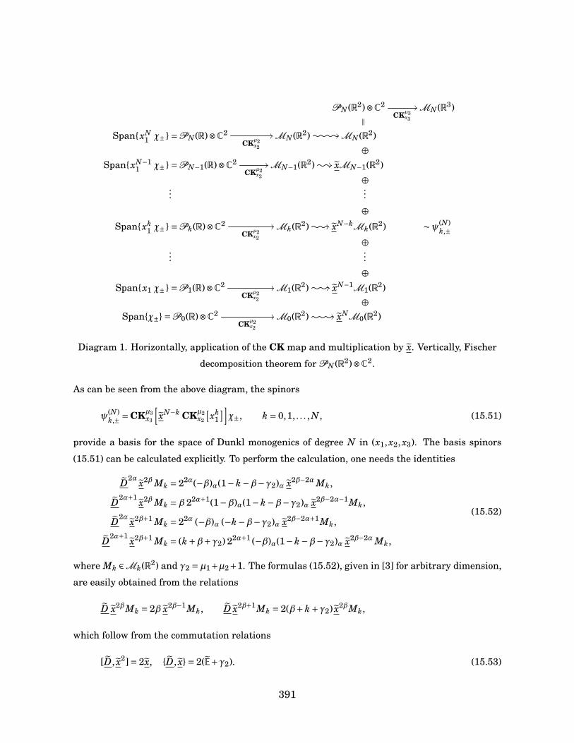
PN (R2)⊗C2CKµ3
x3
//MN (R3)
Span xN1 χ± =PN (R)⊗C2
CKµ2x2
//MN (R2) //MN (R2)∥
Span xN−11 χ± =PN−1(R)⊗C2
CKµ2x2
//MN−1(R2) // xMN−1(R2)
⊕
......
⊕
Span xk1 χ± =Pk(R)⊗C2
CKµ2x2
//Mk(R2) // xN−kMk(R2)
⊕∼ψ(N)
k,±
......
⊕
Span x1 χ± =P1(R)⊗C2CKµ2
x2
//M1(R2) // xN−1M1(R2)
⊕
Spanχ±=P0(R)⊗C2CKµ2
x2
//M0(R2) // xNM0(R2)
⊕
Diagram 1. Horizontally, application of the CK map and multiplication by x. Vertically, Fischer
decomposition theorem for PN (R2)⊗C2.
As can be seen from the above diagram, the spinors
ψ(N)k,± =CKµ3
x3
[xN−k CKµ2
x2
[xk
1]]χ±, k = 0,1, . . . , N, (15.51)
provide a basis for the space of Dunkl monogenics of degree N in (x1, x2, x3). The basis spinors
(15.51) can be calculated explicitly. To perform the calculation, one needs the identities
D2α x2β Mk = 22α(−β)α(1−k−β−γ2)α x2β−2α Mk,
D2α+1 x2β Mk =β 22α+1(1−β)α(1−k−β−γ2)α x2β−2α−1Mk,
D2α x2β+1 Mk = 22α (−β)α (−k−β−γ2)α x2β−2α+1Mk,
D2α+1 x2β+1 Mk = (k+β+γ2) 22α+1 (−β)α(1−k−β−γ2)α x2β−2α Mk,
(15.52)
where Mk ∈Mk(R2) and γ2 =µ1+µ2+1. The formulas (15.52), given in [3] for arbitrary dimension,
are easily obtained from the relations
D x2βMk = 2β x2β−1Mk, D x2β+1Mk = 2(β+k+γ2) x2βMk,
which follow from the commutation relations
[D, x2]= 2x, D, x= 2(E+γ2). (15.53)
391
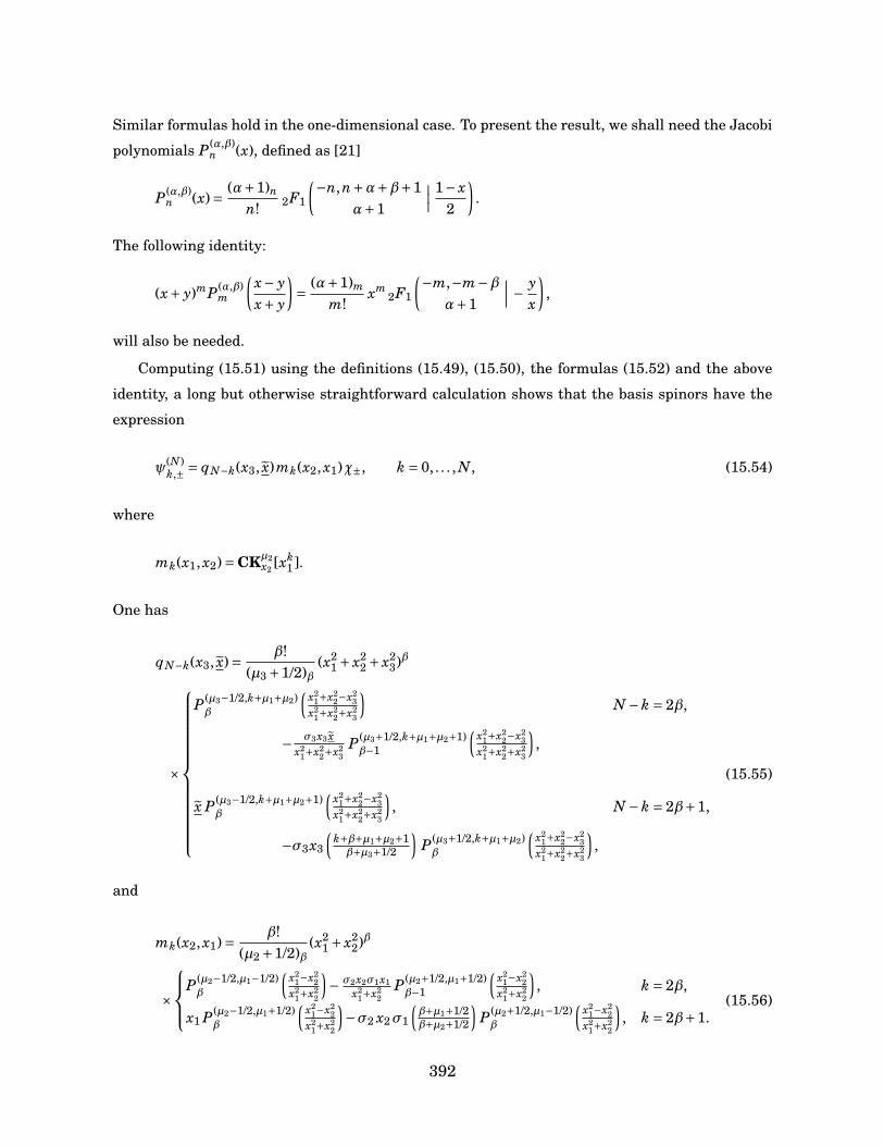
Similar formulas hold in the one-dimensional case. To present the result, we shall need the Jacobi
polynomials P(α,β)n (x), defined as [21]
P(α,β)n (x)= (α+1)n
n! 2F1
(−n,n+α+β+1α+1
∣∣∣ 1− x2
).
The following identity:
(x+ y)mP(α,β)m
(x− yx+ y
)= (α+1)m
m!xm
2F1
(−m,−m−βα+1
∣∣∣ − yx
),
will also be needed.
Computing (15.51) using the definitions (15.49), (15.50), the formulas (15.52) and the above
identity, a long but otherwise straightforward calculation shows that the basis spinors have the
expression
ψ(N)k,± = qN−k(x3, x)mk(x2, x1)χ±, k = 0, . . . , N, (15.54)
where
mk(x1, x2)=CKµ2x2 [xk
1 ].
One has
qN−k(x3, x)= β!(µ3 +1/2)β
(x21 + x2
2 + x23)β
×
P(µ3−1/2,k+µ1+µ2)β
(x2
1+x22−x2
3x2
1+x22+x2
3
)N −k = 2β,
− σ3x3 xx2
1+x22+x2
3P(µ3+1/2,k+µ1+µ2+1)β−1
(x2
1+x22−x2
3x2
1+x22+x2
3
),
x P(µ3−1/2,k+µ1+µ2+1)β
(x2
1+x22−x2
3x2
1+x22+x2
3
), N −k = 2β+1,
−σ3x3
(k+β+µ1+µ2+1β+µ3+1/2
)P(µ3+1/2,k+µ1+µ2)β
(x2
1+x22−x2
3x2
1+x22+x2
3
),
(15.55)
and
mk(x2, x1)= β!(µ2 +1/2)β
(x21 + x2
2)β
×
P(µ2−1/2,µ1−1/2)β
(x2
1−x22
x21+x2
2
)− σ2x2σ1x1
x21+x2
2P(µ2+1/2,µ1+1/2)β−1
(x2
1−x22
x21+x2
2
), k = 2β,
x1 P(µ2−1/2,µ1+1/2)β
(x2
1−x22
x21+x2
2
)−σ2 x2σ1
(β+µ1+1/2β+µ2+1/2
)P(µ2+1/2,µ1−1/2)β
(x2
1−x22
x21+x2
2
), k = 2β+1.
(15.56)
392
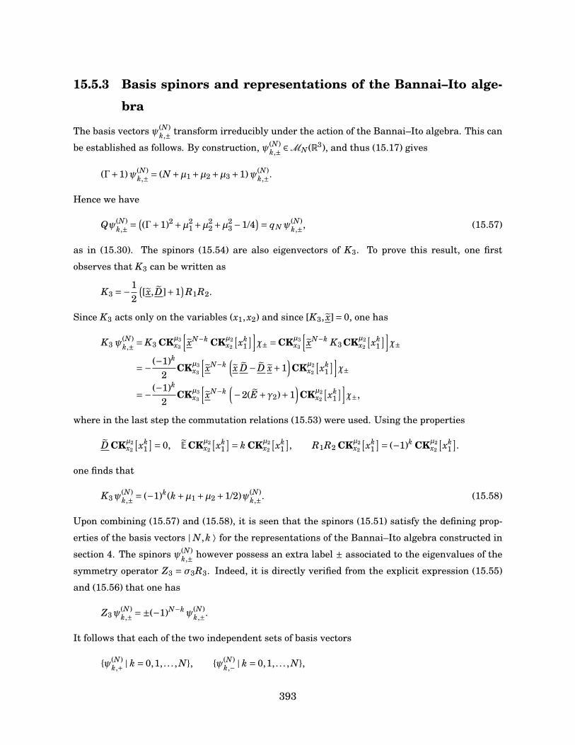
15.5.3 Basis spinors and representations of the Bannai–Ito alge-
bra
The basis vectors ψ(N)k,± transform irreducibly under the action of the Bannai–Ito algebra. This can
be established as follows. By construction, ψ(N)k,± ∈MN (R3), and thus (15.17) gives
(Γ+1)ψ(N)k,± = (N +µ1 +µ2 +µ3 +1)ψ(N)
k,±.
Hence we have
Qψ(N)k,± = (
(Γ+1)2 +µ21 +µ2
2 +µ23 −1/4
)= qN ψ(N)k,±, (15.57)
as in (15.30). The spinors (15.54) are also eigenvectors of K3. To prove this result, one first
observes that K3 can be written as
K3 =−12
([x, D]+1
)R1R2.
Since K3 acts only on the variables (x1, x2) and since [K3, x]= 0, one has
K3 ψ(N)k,± = K3 CKµ3
x3
[xN−k CKµ2
x2
[xk
1]]χ± =CKµ3
x3
[xN−k K3 CKµ2
x2
[xk
1]]χ±
=− (−1)k
2CKµ3
x3
[xN−k
(x D− D x+1
)CKµ2
x2
[xk
1]]χ±
=− (−1)k
2CKµ3
x3
[xN−k
(−2(E+γ2)+1
)CKµ2
x2
[xk
1]]χ±,
where in the last step the commutation relations (15.53) were used. Using the properties
D CKµ2x2
[xk
1]= 0, ECKµ2
x2
[xk
1]= k CKµ2
x2
[xk
1], R1R2 CKµ2
x2
[xk
1]= (−1)k CKµ2
x2
[xk
1].
one finds that
K3ψ(N)k,± = (−1)k(k+µ1 +µ2 +1/2)ψ(N)
k,±. (15.58)
Upon combining (15.57) and (15.58), it is seen that the spinors (15.51) satisfy the defining prop-
erties of the basis vectors | N,k ⟩ for the representations of the Bannai–Ito algebra constructed in
section 4. The spinors ψ(N)k,± however possess an extra label ± associated to the eigenvalues of the
symmetry operator Z3 = σ3R3. Indeed, it is directly verified from the explicit expression (15.55)
and (15.56) that one has
Z3ψ(N)k,± =±(−1)N−kψ(N)
k,±.
It follows that each of the two independent sets of basis vectors
ψ(N)k,+ | k = 0,1, . . . , N, ψ(N)
k,− | k = 0,1, . . . , N,
393
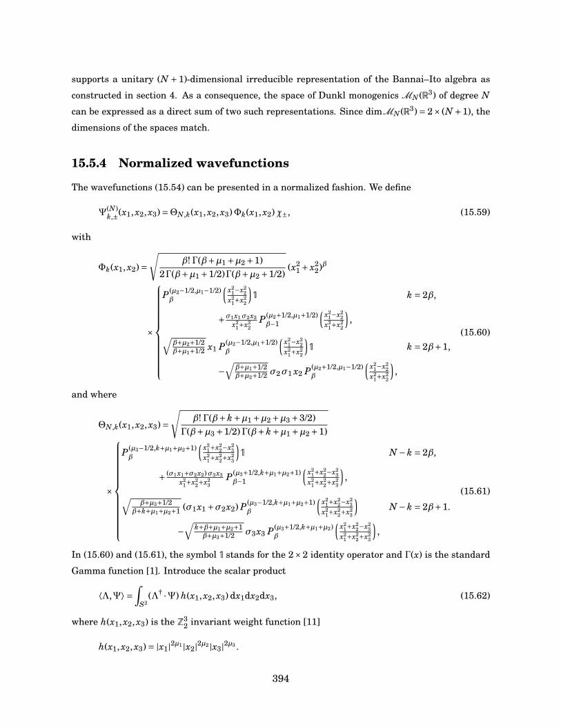
supports a unitary (N +1)-dimensional irreducible representation of the Bannai–Ito algebra as
constructed in section 4. As a consequence, the space of Dunkl monogenics MN (R3) of degree N
can be expressed as a direct sum of two such representations. Since dimMN (R3)= 2× (N +1), the
dimensions of the spaces match.
15.5.4 Normalized wavefunctions
The wavefunctions (15.54) can be presented in a normalized fashion. We define
Ψ(N)k,±(x1, x2, x3)=ΘN,k(x1, x2, x3)Φk(x1, x2) χ±, (15.59)
with
Φk(x1, x2)=√
β!Γ(β+µ1 +µ2 +1)2Γ(β+µ1 +1/2)Γ(β+µ2 +1/2)
(x21 + x2
2)β
×
P(µ2−1/2,µ1−1/2)β
(x2
1−x22
x21+x2
2
)1 k = 2β,
+σ1x1σ2x2x2
1+x22
P(µ2+1/2,µ1+1/2)β−1
(x2
1−x22
x21+x2
2
),√
β+µ2+1/2β+µ1+1/2 x1 P(µ2−1/2,µ1+1/2)
β
(x2
1−x22
x21+x2
2
)1 k = 2β+1,
−√
β+µ1+1/2β+µ2+1/2 σ2σ1 x2 P(µ2+1/2,µ1−1/2)
β
(x2
1−x22
x21+x2
2
),
(15.60)
and where
ΘN,k(x1, x2, x3)=√
β!Γ(β+k+µ1 +µ2 +µ3 +3/2)Γ(β+µ3 +1/2)Γ(β+k+µ1 +µ2 +1)
×
P(µ3−1/2,k+µ1+µ2+1)β
(x2
1+x22−x2
3x2
1+x22+x2
3
)1 N −k = 2β,
+ (σ1x1+σ2x2)σ3x3x2
1+x22+x2
3P(µ3+1/2,k+µ1+µ2+1)β−1
(x2
1+x22−x2
3x2
1+x22+x2
3
),
√β+µ3+1/2
β+k+µ1+µ2+1 (σ1x1 +σ2x2) P(µ3−1/2,k+µ1+µ2+1)β
(x2
1+x22−x2
3x2
1+x22+x2
3
)N −k = 2β+1.
−√
k+β+µ1+µ2+1β+µ3+1/2 σ3x3 P(µ3+1/2,k+µ1+µ2)
β
(x2
1+x22−x2
3x2
1+x22+x2
3
),
(15.61)
In (15.60) and (15.61), the symbol 1 stands for the 2×2 identity operator and Γ(x) is the standard
Gamma function [1]. Introduce the scalar product
⟨Λ,Ψ⟩ =∫
S2(Λ† ·Ψ) h(x1, x2, x3) dx1dx2dx3, (15.62)
where h(x1, x2, x3) is the Z32 invariant weight function [11]
h(x1, x2, x3)= |x1|2µ1 |x2|2µ2 |x3|2µ3 .
394

It is directly verified (see for example [13]) that the spherical Dirac-Dunkl operator Γ and its sym-
metry operators K i, Zi are self-adjoint with respect to the scalar product (15.62). Upon writing the
wavefunctions (15.59) in the spherical coordinates, it follows from the orthogonality relation of the
Jacobi polynomials (see for example [21]) that the wavefunctions (15.59) satisfy the orthogonality
relation
⟨Ψ(N ′)k′, j ,Ψ(N)
k, j′⟩ = δkk′δNN ′δ j j′ .
15.5.5 Role of the Bannai–Ito polynomials
Let us briefly discuss the role played by the Bannai–Ito polynomials in the present picture. It
is known that these polynomials arise as overlap coefficients between the respective eigenbases
of any pair of generators of the Bannai–Ito algebra in the representations (15.30) [17, 27]. We
introduce the basis Υ(N)s,± defined by
Υ(N)s,± = ΘN,s(x2, x3, x1) Φs(x2, x3) χ±, s = 0, . . . , N, (15.63)
where Θ and Φ are obtained from (15.60) and (15.61) by applying the permutation (µ1,µ2,µ3) →(µ2,µ3,µ1). It is easily seen from (15.22) and (15.24) that the wavefunctions (15.63) satisfy the
eigenvalue equations
(Γ+1)Υ(N)s,± = (N +µ1 +µ2 +µ3 +1)Υ(N)
s,± ,
K1Υ(N)s,± = (−1)s(s+µ2 +µ3 +1/2)Υ(N)
s,± ,
σ3R3Υ(N)s,± =±(−1)N−sΥ(N)
s,± .
With the scalar product (15.62), the overlap coefficients between the bases Ψ(N)k,± and Υ(N)
s,± are
defined as
⟨Υ(N)s,q ,Ψ(N)
k,r ⟩ =W (N)s,k;q,r.
The coefficients W (N)s,k;q,r can be expressed in terms of the Bannai–Ito polynomials (see [19]).
15.6 Conclusion
In this paper, we considered the Dirac–Dunkl operator on the two-sphere associated to the Z32
Abelian reflection group. We have obtained its symmetries and shown that they generate the
Bannai–Ito algebra. We have built the relevant representations of the Bannai–Ito algebra using
ladder operators. Finally, using a Cauchy-Kovalevskaia extension theorem, we have constructed
395
the eigenfunctions of the spherical Dirac–Dunkl operator and we have shown that they transform
according to irreducible representations of the Bannai–Ito algebra.
As observed in this paper, the formulas (15.1) can be considered as a three-parameter deforma-
tion of the algebra sl2 and as such, it can be considered to have rank one. It would of great interest
in the future to generalize the Bannai–Ito algebra to arbitrary rank. In that regard, the study of
the Dirac–Dunkl operator in n dimensions associated to the Zn2 reflection group is interesting.
References[1] G. Andrews, R. Askey, and R. Roy. Special functions, volume 71 of Encyclopedia of Mathe-
matics and its Applications. Cambridge University Press, 2001.
[2] H. De Bie, V. X. Genest, S. Tsujimoto, L. Vinet, and A. Zhedanov. The Bannai-Ito algebra and
some applications. Journal of Physics: Conference Series, 2015.
[3] H. De Bie, B. Ørsted, P. Somberg, and V. Soucek. Dunkl operators and a family of realizations
of osp(1|2). Transactions of the American Mathematical Society, 364(7):3875–3902, July 2012.
[4] H. De Bie and N. De Schepper. Clifford-Gegenbauer polynomials related to the Dunkl Dirac
operator. The Bulletin of the Belgian Mathematical Society-Simon Stevin, 18(2):193–214,
May 2011.
[5] F. Brackx, R. Delanghe, and F. Sommen. Clifford analysis. Addison-Wesley, 1982.
[6] P. Cerejeiras, U. Kähler, and G. Ren. Clifford analysis for finite reflection groups. Complex
Variables and Elliptic Equations, 51(5-6):487–495, October 2006.
[7] F. Dai and Y. Xu. Approximation Theory and Harmonic Analysis on Spheres and Balls.
Springer, 2013.
[8] C. Dunkl. Reflection groups and orthogonal polynomials on the sphere. Mathematische
Zeitschrift, 197(13):33–60, 1988.
[9] C. Dunkl. Differential-difference operators associated to reflection groups. Transactions of
the American Mathematical Society, 311(13):167–183, January 1989.
[10] C. Dunkl. Integral kernels with reflection group invariance. Canadian Journal of Mathemat-
ics, 43(6):1213–1227, December 1991.
[11] C. Dunkl and Y. Xu. Orthogonal Polynomials of Several Variables. Cambridge University
Press, 2nd edition, 2014.
396
[12] L. Frappat, A. Sciarrino, and P. Sorba. Dictionary on Lie Algebras and Superalgebras. Aca-
demic Press, 2000.
[13] V. X. Genest, M. Ismail, L. Vinet, and A. Zhedanov. The Dunkl oscillator in the plane: I.
Superintegrability, separated wavefunctions and overlap coefficients . Journal of Physics A:
Mathematical and Theoretical, 46(14):145201, April 2013.
[14] V. X. Genest, M. Ismail, L. Vinet, and A. Zhedanov. The Dunkl Oscillator in the Plane
II: Representations of the Symmetry Algebra. Communications in Mathematical Physics,
329(3):999–1029, August 2014.
[15] V. X. Genest, L. Vinet, and A. Zhedanov. Bispectrality of the Complementary Bannai–Ito
polynomials. SIGMA, 9:18, March 2013.
[16] V. X. Genest, L. Vinet, and A. Zhedanov. The Bannai-Ito algebra and a superintegrable sys-
tem with reflections on the two-sphere. Journal of Physics A: Mathematical and Theoretical,
47(20):205202, May 2014.
[17] V. X. Genest, L. Vinet, and A. Zhedanov. The Bannai-Ito polynomials as Racah coefficients
of the sl−1(2) algebra. Proceedings of the American Mathematical Society, 142(5):1545–1560,
May 2014.
[18] V. X. Genest, L. Vinet, and A. Zhedanov. The Dunkl oscillator in three dimensions. Journal
of Physics: Conference Series, 512(13):012010, 2014.
[19] V. X. Genest, L. Vinet, and A. Zhedanov. A Laplace-Dunkl equation on S2 and the Bannai–Ito
algebra. Communications in Mathematical Physics (in Press), 2015.
[20] P. Graczyk, M. Rösler, and M. Yor, editors. Harmonic and Stochastic Analysis of Dunkl Pro-
cesses. Hermann, 2008.
[21] R. Koekoek, P. A. Lesky, and R. F. Swarttouw. Hypergeometric orthogonal polynomials and
their q-analogues. Springer, 2010.
[22] A. Lesniewski. A remark on the Casimir elements of Lie superalgebras and quantized Lie
superalgebras. Journal of Mathematical Physics, 36(3):1457–1461, March 1995.
[23] B. Ørsted, P. Somberg, and V. Soucek. The Howe duality for the Dunkl version of the Dirac
operator. Advances in Applied Clifford Algebras, 19(2):403–415, July 2009.
[24] M. Rösler. Dunkl Operators: Theory and Applications. In Orthogonal Polynomials and Spe-
cial Functions, volume 1817 of Lecture Notes in Mathematics , pages 93–135. Springer, 2003.
397
[25] M. Rösler and M. Voit. Markov Processes Related with Dunkl Operators. Advances in Applied
Mathematics, 21(4), November 1998.
[26] S. Tsujimoto, L. Vinet, and A. Zhedanov. From slq(2) to a parabosonic Hopf algebra. SIGMA,
7:93–105, 2011.
[27] S. Tsujimoto, L. Vinet, and A. Zhedanov. Dunkl shift operators and Bannai–Ito polynomials.
Advances in Mathematics, 229(4):2123–2158, March 2012.
[28] L. Vinet and J. F. Van Diejen, editors. Calogero-Moser-Sutherland models. Springer, 2000.
398
Partie III
Tableau de Bannai–Ito etstructures algébriques associées
399

Introduction
L’une des avancées récentes dans la théorie des polynômes orthogonaux est la découverte de
plusieurs nouvelles familles de polynômes orthogonaux hypergéométriques qui correspondent à
des limites q →−1 des q-polynômes du tableau de Askey [60, 61, 62, 63]. Tout comme les polynômes
du tableau de Askey, les polynômes «−1 » peuvent être organisés au sein d’une hiérarchie appelée
tableau de Bannai–Ito, dont la construction n’est toujours pas achevée. Au sommet de cette hiérar-
chie trônent les familles des polynômes de Bannai–Ito et des polynômes de Bannai–Ito complémen-
taires, qui dépendent chacune de quatre paramètres. Ces deux familles ont plusieurs descendants
qui s’obtiennent à partir de limites ou de spécialisations. À l’instar des polynômes du tableau de
Askey, les polynômes du tableau de Bannai-Ito sont bispectraux. Une famille de polynômes or-
thogonaux Pn(x) est dite bispectrale si en plus d’obéir à la relation de récurrence à trois termes
caractéristique de tous les polynômes orthogonaux
xPn(x)= Pn+1(x)+bnPn(x)+ cnPn−1(x),
où P−1(x) = 0 et P0(x) = 1 et où bn, cn sont des suites de nombres, elle satisfait aussi à une
équation aux valeurs propres
L Pn(x)=λnPn(x),
où L est un opérateur différentiel, aux différences ou aux q-différences. La propriété de bis-
pectralité d’une famille de polynômes orthogonaux est importante du point de vue de ses appli-
cations physiques potentielles: tous les polynômes orthogonaux qui apparaissent dans un cadre
physique sont bispectraux. La caractéristique qui distingue les polynômes −1 de ceux du tableau
d’Askey est que les opérateurs L qu’ils diagonalisent font intervenir des opérateurs de réflexion
RPn(x)= Pn(−x).
Dans cette partie de la thèse, on étudie plusieurs familles de polynômes −1 et on examine
les structures algébriques qui leurs sont associées. On démontre d’abord la bispectralité des
polynômes de Bannai–Ito complémentaires. On définit ensuite une nouvelle famille de polynômes
−1 appelés polynômes de Chihara, que l’on caractérise. Puis, on montre que les polynômes de
Bannai–Ito sont les coefficients de Racah de l’algèbre osp(1|2). Ceci nous conduit à examiner la
401
structure algébrique qui est associée aux polynômes duaux −1 de Hahn dans le contexte du pro-
blème de Clebsch-Gordan de osp(1|2). On propose une q-déformation des polynômes de Bannai–Ito
en considérant les coefficients de Racah de la superalgèbre quantique ospq(1|2). Finalement, on
montre que l’algèbre associée aux q-polynômes de Bannai–Ito, appelée algèbre de q-Bannai–Ito,
sert d’algèbre de covariance pour ospq(1|2).
402
Chapitre 16
Bispectrality of the ComplementaryBannai–Ito polynomials
V. X. Genest, L. Vinet et A. Zhedanov (2013). Bispectrality of the Complementary Bannai–Ito
polynomials. SIGMA 9 18-37
Abstract. A one-parameter family of operators that have the Complementary Bannai–Ito (CBI)
polynomials as eigenfunctions is obtained. The CBI polynomials are the kernel partners of the
Bannai–Ito polynomials and also correspond to a q →−1 limit of the Askey-Wilson polynomials.
The eigenvalue equations for the CBI polynomials are found to involve second order Dunkl shift
operators with reflections and exhibit quadratic spectra. The algebra associated to the CBI poly-
nomials is given and seen to be a deformation of the Askey-Wilson algebra with an involution.
The relation between the CBI polynomials and the recently discovered dual −1 Hahn and para-
Krawtchouk polynomials, as well as their relation with the symmetric Hahn polynomials, is also
discussed.
16.1 Introduction
One of the recent advances in the theory of orthogonal polynomials (OPs) has been the discovery
of several new families of ”classical” OPs that correspond to q → −1 limits of q-polynomials of
the Askey scheme [20, 22, 25, 26]. The word ”classical” here refers to the fact that in addition to
obeying the three-term relation
Pn+1(x)+βnPn(x)+γnPn−1(x)= xPn(x),
the polynomials Pn(x) also satisfy an eigenvalue equation of the form
L Pn(x)=λnPn(x).
403
The novelty of these families of −1 orthogonal polynomials lies in the fact that for each family the
operator L is a differential or difference operator that also contains the reflection operator R f (x)=f (−x) [24]. Such differential/difference operators are said to be of Dunkl type [4], notwithstanding
the fact that the operators L differ from the standard Dunkl operators in that they preserve the
linear space of polynomials of any given maximal degree. In this connection, these −1 OPs have
also been referred to as Dunkl orthogonal polynomials.
With the discovery and characterization of these Dunkl polynomials, a −1 scheme of OPs,
completing the Askey scheme, is beginning to emerge. At the top of the discrete variable branch
of this −1 scheme lie two families of orthogonal polynomials: the Bannai–Ito (BI) polynomials and
their kernel partners the Complementary Bannai–Ito polynomials (CBI); both families correspond
to different q →−1 limits of the Askey-Wilson polynomials.
The Bannai–Ito polynomials were originally identified by Bannai and Ito themselves in [1]
where they recognized that these OPs correspond to the q →−1 limit of the q-Racah polynomials.
However, it is only recently [22] that the Dunkl shift operator L admitting the BI polynomials
as eigenfunctions has been constructed. The BI polynomials and their special cases enjoy the
Leonard duality property, a property they share with all members of the discrete part of the Askey
scheme [1, 14]. This means that in addition to satisfying a three-term recurrence relation, the
BI polynomials also obey a three-term difference equation. From the algebraic point of view, this
property corresponds to the existence of an associated Leonard pair [17].
Amongst the discrete-variable −1 polynomials, there are families that do not possess the Leo-
nard duality property. That is the case of the Complementary Bannai-Ito polynomials and their
descendants [20, 22]. This situation is connected to the fact that in these cases the difference oper-
ator of the corresponding q-polynomials do not admit a q →−1 limit. In [20], a five-term difference
equation was nevertheless constructed for the dual −1 Hahn polynomials and the defining Dunkl
operator for these polynomials was found.
In this paper, a one-parameter family of Dunkl operators Dα of which the Complementary
Bannai–Ito polynomials are eigenfunctions is derived, thus establishing the bispectrality of the
CBI polynomials. The operators of this family involve reflections and are of second order in
discrete shifts; they are diagonalized by the CBI polynomials with a quadratic spectrum. The
corresponding five-term difference equation satisfied by the CBI polynomials is presented. More-
over, an algebra associated to the CBI polynomials is derived. This quadratic algebra, called the
Complementary Bannai–Ito algebra, is defined in terms of four generators. It can be seen as a
deformation with an involution of the quadratic Hahn algebra QH(3) [8, 30], which is a special
case of the Askey-Wilson AW(3) algebra [18, 29].
The paper, which provides a comprehensive description of the CBI polynomials and their prop-
erties, is organized in the following way. In Section 1, we present a review of the Bannai–Ito
404
polynomials. In Section 2, we define the Complementary Bannai–Ito polynomials and obtain their
recurrence and orthogonality relations. In Section 3, we use a proper q →−1 limit of the Askey-
Wilson difference operator to construct an operator D of which the CBI polynomials are eigen-
functions. We use a ”hidden” eigenvalue equation to show that one has in fact a one-parameter
family of operators Dα, parametrized by a complex number α, that is diagonalized by the CBI
polynomials. In Section 4, we derive the CBI algebra and present some aspects of its irreducible
representations. In Section 5, we discuss the relation between the CBI polynomials and three
other families of OPs: the dual −1 Hahn, the para-Krawtchouk and the classical Hahn polynomi-
als; these OP families are respectively a limit and two special cases of the CBI polynomials. We
conclude with a perspective on the continuum limit and an outlook.
16.2 Bannai–Ito polynomials
The Bannai–Ito polynomials were introduced in 1984 [1] in the complete classification of orthogo-
nal polynomials possessing the Leonard duality property (see Section 4). It was shown that they
can be obtained as a q →−1 limit of the q-Racah polynomials and some of their properties were
derived. Recently [22], it was observed that the BI polynomials also occur as eigensolutions of
a first order Dunkl shift operator. In the following, we review some of the properties of the BI
polynomials; we use the presentation of [22].
The monic BI polynomials Bn(x;ρ1,ρ2, r1, r2), denoted Bn(x) for notational convenience, satisfy
the three-term recurrence relation
Bn+1(x)+ (ρ1 − An −Cn)Bn(x)+ An−1CnBn−1(x)= xBn(x), (16.1)
with the initial conditions B−1(x) = 0 and B0(x) = 1. The recurrence coefficients An and Cn are
given by
An =
(n+2ρ1−2r1+1)(n+2ρ1−2r2+1)
4(n+g+1) , neven,(n+2g+1)(n+2ρ1+2ρ2+1)
4(n+g+1) , nodd,(16.2a)
Cn =
− n(n−2r1−2r2)4(n+g) , neven,
− (n+2ρ2−2r2)(n+2ρ2−2r1)4(n+g) , nodd,
(16.2b)
where
g = ρ1 +ρ2 − r1 − r2.
It is seen from the above formulas that the positivity condition un = An−1Cn > 0 cannot be satisfied
for all n ∈ N [3]. Hence it follows that the Bannai–Ito polynomials can only form a finite set of
405
positive-definite orthogonal polynomials B0(x), . . . ,BN (x), which occurs when the ”local” positivity
condition ui > 0 for i ∈ 1, . . . , N and the truncation conditions u0 = 0, uN+1 = 0 are satisfied. If
these conditions are fulfilled, the BI polynomials Bn(x) satisfy the discrete orthogonality relation
N∑k=0
wkBn(xk)Bm(xk)= hnδnm,
with respect to the positive weight wk. The spectral points xk are the simple roots of the polyno-
mial BN+1(x). The explicit formulae for the weight function wk and the grid points xk depend on
the realization of the truncation condition uN+1 = 0.
If N is even, it follows from (16.2) that the condition uN+1 = 0 is tantamount to one of the
following requirements:
1) r1 −ρ1 = N +12
, 2) r2 −ρ1 = N +12
,
3) r1 −ρ2 = N +12
, 4) r2 −ρ2 = N +12
.
For the cases 1) and 2), the grid points have the expression
xk = (−1)k(k/2+ρ1 +1/4)−1/4, (16.3)
and the weights take the form
wk =(−1)ν
`!(ρ1 − r1 +1/2)`+ν(ρ1 − r2 +1/2)`+ν(ρ1 +ρ2 +1)`(2ρ1 +1)`
(ρ1 + r1 +1/2)`+ν(ρ1 + r2 +1/2)`+ν(ρ1 −ρ2 +1)`, (16.4)
where one has k = 2`+ν with ν ∈ 0,1 and where (a)n = a(a+1) · · · (a+n−1) is the Pochhammer
symbol. For the cases 3) and 4), the formulae (16.3) and (16.4) hold under the substitution ρ1 ↔ ρ2.
If N is odd, it follows from (16.2) that the condition uN+1 = 0 is equivalent to one of the follow-
ing restrictions:
i)ρ1 +ρ2 =−N +12
, ii) r1 + r2 = N +12
, iii)ρ1 +ρ2 − r1 − r2 =−N +12
.
The condition iii) leads to a singularity in un when n = (N +1)/2 and hence only the conditions i)
and ii) are admissible. For the case i), the formulae (16.3) and (16.4) hold under the substitution
ρ1 ↔ ρ2. For the case ii), the spectral points are given by
xk = (−1)k(r1 −k/2−1/4)−1/4,
and the weight function is given by (16.4) with the substitutions (ρ1,ρ2, r1, r2)→−(r1, r2,ρ1,ρ2).
The Bannai–Ito polynomials can be obtained from a q →−1 limit of the Askey-Wilson polyno-
mials and also have the Bannai–Ito algebra as their characteristic algebra (see [7] and [22]).
406
16.3 CBI polynomials
In this section we define the Complementary Bannai–Ito polynomials through a Christoffel trans-
formation of the Bannai–Ito polynomials. We derive their recurrence relation, hypergeometric
representation and orthogonality relations from their kernel properties.
The Complementary Bannai–Ito polynomials In(x;ρ1,ρ2, r1, r2), denoted In(x) for convenience,
are defined from the BI polynomials Bn(x) by the transformation [22]
In(x)= Bn+1(x)− AnBn(x)x−ρ1
, (16.5)
where An is as in (16.2). The transformation (16.5) is an example of a Christoffel transformation
[16]. It is easily seen from the definition (16.5) that In(x) is a monic polynomial of degree n in x.
The inverse relation for the CBI polynomials is given by a Geronimus [31] transformation and has
the expression
Bn(x)= In(x)−CnIn−1(x). (16.6)
This formula can be verified by direct substitution of (16.5) in (16.6) which yields back the defining
relation (16.1) of the BI polynomials. In the reverse, the substitution of (16.6) in (16.5) yields the
three-term recurrence relation [11]
In+1(x)+ (ρ1 − An −Cn+1)In(x)+ AnCn In−1(x)= xIn(x), (16.7)
where An and Cn are given by (16.2). The recurrence relation (16.7) can be written explicitly as
In+1(x)+ (−1)nρ2 In(x)+τnIn−1(x)= xIn(x), (16.8)
where τn is given by
τ2n =−n(n+ρ1 − r1 +1/2)(n+ρ1 − r2 +1/2)(n− r1 − r2)(2n+ g)(2n+ g+1)
, (16.9a)
τ2n+1 =− (n+ g+1)(n+ρ1 +ρ2 +1)(n+ρ2 − r1 +1/2)(n+ρ2 − r2 +1/2)(2n+ g+1)(2n+ g+2)
, (16.9b)
and where g = ρ1 +ρ2 − r1 − r2. One has also the initial conditions I0 = 1 and I1 = x−ρ2.
The CBI polynomials are kernel polynomials of the BI polynomials. Indeed, by noting
that
An = Bn+1(ρ1)/Bn(ρ1),
which follows by induction from (16.1), the transformation (16.5) may be cast in the form
In(x)= (x−ρ1)−1[Bn+1(x)− Bn+1(ρ1)
Bn(ρ1)Bn(x)
]. (16.10)
407
It is manifest from (16.10) that In(x) are the kernel polynomials associated to Bn(x) with
kernel parameter ρ1 [3]. Since the BI polynomials Bn(x) are orthogonal with respect to a
linear functional σ(i):
⟨σ(i),Bn(x)Bm(x)⟩ = 0, n 6= m,
where the upper index on σ(i) designates the possible functionals associated to the various
truncation conditions, it follows from (16.10) that we have [3]
⟨σ(i), (x−ρ1)In(x)Im(x)⟩ = 0, n 6= m. (16.11)
Hence the orthogonality and positive-definiteness of the CBI polynomials can be studied
using the formulae (16.9) and (16.11) .
It is seen from (16.9) that the condition τn > 0 cannot be ensured for all n and hence
the Complementary Bannai–Ito polynomials can only form a finite system of positive-
definite orthogonal polynomials I0(x), . . . , IN(x), provided that the ”local” positivity τn > 0,
n ∈ 1, . . . , N, and truncation conditions τ0 = 0 and τN+1 = 0 are satisfied.
When N is even, the truncation conditions τ0 = 0 and τN+1 = 0 are equivalent to one
of the four prescriptions
1)ρ2 − r1 =−N +12
, 2)ρ2 − r2 =−N +12
, (16.12a)
3)ρ1 +ρ2 =−N +22
, 4) g =−N +22
. (16.12b)
Since the condition 4) leads to a singularity in τn, only the conditions 1), 2) and 3) are
admissible. For all three conditions and assuming that the positivity conditions are sat-
isfied, the CBI polynomials enjoy the orthogonality relation
N∑k=0
wkIn(xk)Im(xk)= hnδnm, (16.13)
where the spectral points are given by
xk = (−1)k(k/2+ρ2 +1/4)−1/4
and the positive weights are
wk = (xk −ρ1)wk,
with wk defined by (16.4) with the substitution ρ1 ↔ ρ2.
408
When N is odd, the truncation conditions τ0 = 0 and τN+1 = 0 are tantamount to
i) r1 −ρ1 = N +22
, ii) r1 + r2 = N +12
, iii) r2 −ρ1 = N +22
. (16.14)
If the positivity condition τn > 0 is satisfied for n ∈ 1, . . . , N, the CBI polynomials will en-
joy the orthogonality relation (16.13) with respect to the positive definite weight function
wk. When either condition i) or ii) is satisfied, the spectral points are given by
xk = (−1)k(r1 −k/2−1/4)−1/4,
together with the weight function wk = (xk −ρ1)wk where wk is given by (16.4) with the
replacement (ρ1,ρ2, r1, r2) = −(r1, r2,ρ1,ρ2). Finally, the orthogonality relation for the
truncation condition iii) is obtained from the preceding case under the exchange r1 ↔ r2.Let us now illustrate when positive-definiteness occurs for the CBI polynomials. We
first consider the even N case. It is sufficient to take
ρ1 =( a+b
2 + c+N2
), ρ2 =
( a+b2 −1
2
), r1 =
( a+b2 +N
2
), r2 =
(a−b
4
), (16.15)
where a, b and c are arbitrary positive parameters. Assuming (16.15), the recurrence
coefficients (16.9) become
τn =
n(N−n+a)(n+c+1)(n+b+c+N+1)
16(n+g)(n+g+1) , neven,(N−n+1)(n+b−1)(n+b+c)(n+a+b+c+N)
16(n+g)(n+g+1) , nodd,(16.16)
where g = (b+ c−1)/2. It is obvious from (16.16) that the positivity and truncation condi-
tions are satisfied for n ∈ 1, . . . , N; this corresponds to the case 1) of (16.12).Consider the situation when N > 1 is odd. We introduce the parametrization
ρ1 =(ζ+ξ
2 +χ+N2
), ρ2 =
(ζ−ξ
4
), r1 =
(ζ+ξ
2 +N +12
), r2 =−
(ζ+ξ
4
), (16.17)
where ζ, ξ and χ are arbitrary positive parameters. The recurrence coefficients become
τn =
n(N−n+1)(n+χ)(n+ζ+ξ+χ+N+1)
16(n+g)(n+g+1) , neven,(N−n+ξ+1)(n+ζ)(n+ζ+χ)(n+ζ+χ+N+1)
16(n+g)(n+g+1) , nodd,(16.18)
with g = (ζ+χ−1)/2. Assuming (16.17), the positivity and truncation conditions are man-
ifestly fulfilled; this corresponds to the condition ii) of (16.14). The other cases can be
treated in similar fashion.
409
It is possible to derive a hypergeometric representation for the CBI polynomials using
a method [22, 26] which is analogous to Chihara’s construction of symmetric orthogonal
polynomials [3] and closely related to the scheme developed in [15] (see also [2]). Given
the three-term recurrence relation (16.8), it follows by induction that the polynomials
In(x) can be written as
I2n = Rn(x2), I2n+1 = (x−ρ2)Qn(x2), (16.19)
where Rn(x2) and Qn(x2) are monic polynomials of degree n. It follows directly from
(16.19) and (16.8) that the polynomials Rn(x2) and Qn(x2) obey the following system of
recurrence relations
Rn(z)=Qn(z)+τ2nQn−1(z), (z−ρ22)Qn(z)= Rn+1(z)+τ2n+1Rn(z).
This system is equivalent to the following pair of equations:
Rn+1(z)+ (ρ22 +τ2n +τ2n+1)Rn(z)+τ2n−1τ2nRn−1(z)= zRn(z),
Qn+1(z)+ (ρ22 +τ2n+1 +τ2n+2)Qn(z)+τ2nτ2n+1Qn−1(z)= zQn(z).
These recurrence relations can be identified with those of the Wilson polynomials [13].
From this identification, we obtain
Rn(x2)= ηn 4F3
[ −n,n+ g+1,ρ2 + x,ρ2 − xρ1 +ρ2 +1,ρ2 − r1 +1/2,ρ2 − r2 +1/2
;1], (16.20a)
Qn(x2)= ιn 4F3
[ −n,n+ g+2,ρ2 +1+ x,ρ2 +1− xρ1 +ρ2 +2,ρ2 − r1 +3/2,ρ2 − r2 +3/2
;1], (16.20b)
where pFq denotes the generalized hypergeometric function [5] and where the normaliza-tion coefficients, which ensure that the polynomials are monic, are given by
ηn = (ρ1 +ρ2 +1)n(ρ2 − r1 +1/2)n(ρ2 − r2 +1/2)n
(n+ g+1)n,
ιn = (ρ1 +ρ2 +2)n(ρ2 − r1 +3/2)n(ρ2 − r2 +3/2)n
(n+ g+2)n.
Thus the monic CBI polynomials have the hypergeometric representation (16.19). For
definiteness and future reference, let us now gather the preceding results in the following
proposition.
Proposition 2. The Complementary Bannai–Ito polynomials In(x;ρ1,ρ2, r1, r2) are the
kernel polynomials of the Bannai–Ito polynomials Bn(x;ρ1,ρ2, r1, r2) with kernel parame-
ter ρ1. The monic CBI polynomials obey the three-term recurrence relation
In+1(x)+ (−1)nρ2In(x)+τnIn−1(x)= xIn(x),
410
where τn is given by (16.9). They have the explicit hypergeometric representation
I2n(x)= Rn(x2), I2n+1(x)= (x−ρ2)Qn(x2),
where Rn(x2) and Qn(x2) are as specified by (16.20). If the truncation condition τN+1 = 0
and the positivity condition τn > 0, n ∈ 1, . . . , N, are satisfied, the CBI polynomials obey
the orthogonality relation
N∑k=0
wkIn(xk)Im(xk)= hnδnm,
with respect to the positive weights wk. The grid points xk correspond to the simple roots
of the polynomial IN+1(x). The formulas for the weights and grid points depend on the
truncation condition. With wk(ρ1,ρ2, r1, r2) given as in (16.4), one has
1. For r1 = N+12 +ρ2, r2 = N+1
2 +ρ2 or ρ1 =−N+22 −ρ2 with N even:
xk = (−1)k(ρ2 +k/2+1/4)−1/4, wk = (xk −ρ1)wk(ρ2,ρ1, r1, r2).
2. For r1 = N+22 +ρ1 or r1 = N+1
2 − r2 with N odd:
xk = (−1)k(r1 −k/2−1/4)−1/4, wk = (xk −ρ1)wk(−r1,−r2,−ρ1,−ρ2).
3. For r2 = N+22 +ρ1 with N odd:
xk = (−1)k(r2 −k/2−1/4)−1/4, wk = (xk −ρ1)wk(−r2,−r1,−ρ1,−ρ2).
Proof. The proof follows from the above considerations.
Note that the normalization factor hn appearing in (16.13) can easily be evaluated in
terms of the product τ1τ2 · · ·τn.
The Complementary Bannai–Ito polynomials can be obtained from the Askey-Wilson
polynomials upon taking the q →−1 limit [22]. Consider the Askey-Wilson polynomials
[13] pn(z;a,b, c,d)
pn(z;a,b, c,d)= a−n(ab,ac,ad; q)n 4φ3
( q−n abcdqn−1 az az−1
ab ac ad
∣∣∣q ; q), (16.21)
where φ denotes the basic generalized hypergeometric function [5]. These polynomials
depend on the argument x = (z+ z−1)/2 and on four complex parameters a, b, c and d.
They obey the recurrence relation [13]
αn pn+1(z)+ (a+a−1 −αn −γn)pn(z)+γn pn−1(z)= (z+ z−1)pn(z), (16.22)
411
where the coefficients are
αn = (1−abqn)(1−acqn)(1−adqn)(1−abcdqn−1)a(1−abcdq2n−1)(1−abcdq2n)
,
γn = a(1− qn)(1−bcqn−1)(1−bdqn−1)(1− cdqn−1)(1−abcdq2n−2)(1−abcdq2n−1)
.
To recover the CBI polynomials, we consider the parametrization
a = ieε (2ρ1+3/2), b =−ieε (2ρ2+1/2), c = ieε (−2r2+1/2), d = ieε (−2r1+1/2), (16.23a)
q =−eε, z = ie−2εy. (16.23b)
It can be verified that the limit q →−1 of the Askey-Wilson polynomials
limq→−1
pn(z)= p∗n(y),
exists [22] and that p∗n(y) is a polynomial of degree n in the variable y. Dividing the
recurrence relation (16.22) by 1+ q and taking the limit ε→ 0, which amounts to taking
q →−1, one finds that the recurrence relation of the limit polynomials p∗n(y) is
α∗n p∗
n+1(y)+ (−1)nρ2 p∗n(y)+γ∗n p∗
n−1(y)= (y−1/4)p∗n(y)
where
α∗2n =− (n+ρ1 +ρ2 +1)(n+ g+1)
(2n+ g+1), α∗
2n+1 =− (n+ρ1 − r1 +3/2)(n+ρ1 − r2 +3/2)(2n+ g+2)
, (16.24a)
γ∗2n = n(n− r1 − r2)(2n+ g+1)
, γ∗2n+1 =(n+ρ2 − r1 +1/2)(n+ρ2 − r2 +1/2)
(2n+ g+2). (16.24b)
From (16.9) and (16.24), one has the identification
p∗n(y)= In(y−1/4), (16.25)
where p∗n are the monic version of the limit polynomials p∗
n(y). Consequently, the CBI
polynomial correspond to a q →−1 limit of the Askey-Wilson polynomials, up to a shift in
argument. This property will be used in the next section to construct a Dunkl operator
that has the CBI polynomials as eigenfunctions.
16.4 Bispectrality of CBI polynomials
In this section, we obtain a family of second order Dunkl shift operators for which the
Complementary Bannai–Ito polynomials are eigenfunctions with eigenvalues quadratic
412

in n. This family will be constructed from a limit of a quadratic combination of the Askey-
Wilson q-difference operator. We shall refer to these operators as the defining operators
of the CBI polynomials.
Consider the Askey-Wilson polynomials pn(x) defined by (16.21). They obey the q-
difference equation [13](Ω(z)Ez,q +Ω(z−1)Ez,q−1 − (Ω(z)+Ω(z−1))I
)pn(z)=Λn pn(z), (16.26)
where Ez,q f (z)= f (qz) is the q-shift operator and I denotes the identity. The lhs of (16.26)
is the Askey-Wilson operator. The eigenvalues take the form
Λn = (q−n −1)(1−abcdqn−1),
and the coefficient Ω(z) is given by
Ω(z)= (1−az)(1−bz)(1− cz)(1−dz)(1− z2)(1− qz2)
.
We now consider the limiting form of the q-difference equation (16.26) when q → −1.
As done previously, we choose the parametrization (16.23), which correspond to the CBI
polynomials. We already showed that the Askey-Wilson polynomials pn(z) become the
Complementary Bannai–Ito polynomials p∗n(y). In the limit q →−1, the q-shift operation
pn(z)→ pn(qz) becomes p∗n(y)→ p∗
n(−y+1/2) while pn(z)→ pn(q−1z) is reduced to p∗n(y)→
p∗n(−y−1/2).
It is natural to expect that in the limit q →−1, the equation (16.26) will yield a defin-
ing operator for the CBI polynomials. However a direct computation shows that the limit
ε→ 0 of the equation (16.26) with the parametrization (16.23) does not exist. It is hence
impossible to find the desired operator for the CBI polynomials directly from a limiting
procedure on equation (16.26). Nevertheless, it is possible to work around this difficulty
by choosing an appropriate quadratic combination of the Askey-Wilson operator that sur-
vives the limit q →−1. A similar procedure was used in [20] to establish the bispectrality
of the dual −1 Hahn polynomials.
Let O denote the Askey-Wilson operator
O =Ω(z)Ez,q +Ω(z−1)Ez,q−1 − (Ω(z)+Ω(z−1))I,
which acts on the space of functions f (z) of argument z. We consider the following
quadratic combination
T = c(2)O2 + c(1)O , (16.27)
413

with
c(2) = 116(1+ q)2 , c(1) = 1
4
(1
(q+1)2 − g+1q+1
),
where g = ρ1 + ρ2 − r1 − r2. Since the operator O acts diagonally on the Askey-Wilson
polynomials, we have
T pn(z)= (c(2)Λ2n + c(1)Λn)pn(x). (16.28)
Upon taking the limit ε→ 0 with the parametrization (16.23), the relation (16.28) becomes
Φ1(y)p∗n(y+1)+
Φ5(y)−Φ2(y)−Φ3(y)p∗
n(1/2− y)+Φ3(y)−Φ4(y)−Φ5(y)
p∗
n(y)
+Φ4(y)−Φ1(y)
p∗
n(−y−1/2)+Φ2(y)p∗n(y−1)= κn p∗
n(y) (16.29)
where the eigenvalues are
κ2n = n2 + (g+1)n, κ2n+1 = n2 + (g+2)n+ g2 +2g+5/4.
The coefficients Φi(y) are given by
Φ1(y)= (y+ρ1 +3/4)(y+ρ2 +3/4)(y− r1 +1/4)(y− r2 +1/4)4(y+1/4)(y+3/4)
,
Φ2(y)= (y−ρ1 −5/4)(y−ρ2 −1/4)(y+ r1 −3/4)(y+ r2 −3/4)4(y−1/4)(y−3/4)
,
Φ3(y)= (y+ρ1 +3/4)(y−ρ2 −1/4)(y− r1 +1/4)(y− r2 +1/4)4(y−1/4)(y+1/4)
,
Φ4(y)= (y+ρ1 +3/4)(y+ρ2 −1/4)(y− r1 +1/4)(y− r2 +1/4)4(y−1/4)(y+1/4)
,
Φ5(y)= (y−ρ2 −1/4)4(y−1/4)
2y2 − y+ν
,
where ν takes the form
ν= r1 + r2 +2r1r2 −2ρ1 −2(r1 + r2)ρ1 −4ρ2 +1/8−2g2.
By the identification (16.25), the relation (16.29) gives the Complementary Bannai–Ito
polynomials In(x) as eigenfunctions of a second order Dunkl shift operator, hence estab-
lishing their bispectrality property. In operator form, the equation (16.29) may be rewrit-
ten as
H In(y−1/4)= κnIn(y−1/4),
414
where H has the expression
H =Φ1T1 + (Φ4 −Φ1)T1/2R+ (Φ3 −Φ4 −Φ5)I+ (Φ5 −Φ2 −Φ3)T−1/2R+Φ2T−1,
where Th f (y)= f (y+h) and R f (y)= f (−y). Upon applying the unitary transformation
H = T1/4H T−1/4,
on the operator H and changing the variable from y to x, the eigenvalue equation (16.29)
for the CBI polynomials becomes
H In(x)= κnIn(x),
where we have
H = Φ1T++ (Φ4 − Φ1)T+R+ (Φ3 − Φ4 − Φ5)I+ (Φ5 − Φ2 − Φ3)R+ Φ2T−, (16.30)
with T+ = T1 and T− = T− the usual shift operators in x. The coefficients now have the
expression
Φi =Φi(x+1/4).
We now turn to the study of the uniqueness of the operator H which defines the
eigenvalue equation of the Complementary Bannai–Ito polynomials (apart from trivial
affine transformations). Quite strikingly, a one-parameter family of such operators can
be constructed. This peculiarity is due to the presence of a ”hidden” symmetry in the CBI
polynomials. To see this, we recall the relation (16.19) for the CBI polynomials
I2n = Rn(x2), I2n+1 = (x−ρ2)Qn(x2),
where Rn(x2) and Qn(x2) are monic polynomials of degree n. From the above relation, it
is easily seen that
I2n(−x)= I2n(x), and I2n+1(−x)= (x+ρ2)(ρ2 − x)
I2n+1(x).
The above equations are equivalent to the following non-trivial "hidden" eigenvalue equa-
tion for the CBI polynomials
(ρ2 − x)2x
(In(−x)− In(x)
)=µnIn(x),
415
where µ2n = 0 and µ2n+1 = 1. In operator form, we write
(x−ρ2)2x
(I−R
)In(x)=U In(x)=µnIn(x). (16.31)
The equation (16.31) indicates that adding αU to the operator (16.30) will give another
eigenvalue equation for the Complementary Bannai–Ito polynomials. The modified oper-
ator
H ′ = H +αU ,
will have the same spectrum as H in the even sector; in the odd sector, the eigenvalues
will differ by the constant parameter α.
For definiteness and future reference, let us now collect the preceding results in the
following theorem.
Theorem 1. Let D0 be the second order Dunkl shift operator acting on the space of func-
tions f (x) of argument x
D0 = A(x)T++B(x)T−+C(x)R+D(x)T+R− (A(x)+B(x)+C(x)+D(x))I, (16.32)
where T± f (x)= f (x±1) and R f (x)= f (−x), with the coefficients
A(x)= (x+ρ1 +1)(x+ρ2 +1)(2x−2r1 +1)(2x−2r2 +1)8(x+1)(2x+1)
,
B(x)= (x−ρ2)(x−ρ1 −1)(2x+2r1 −1)(2x+2r2 −1)8x(2x−1)
,
C(x)= (x−ρ2)(4x2 +ω)8x
− (x−ρ2)(x+ρ1 +1)(2x−2r1 +1)(2x−2r2 +1)8x(2x+1)
−B(x),
D(x)= ρ2(x+ρ1 +1)(2x−2r1 +1)(2x−2r2 +1)8x(x+1)(2x+1)
,
and with
ω= 4ρ1 −4(r1 + r2)ρ1 +4r1r2 −6(r1 + r2)+5.
Furthermore, let α ∈C be a complex number and denote the monic Complementary Bannai-
Ito polynomials by In(x). Then the following eigenvalue equation is satisfied:
DαIn(x)=Λ(α)n In(x), (16.33)
where the eigenvalues are
Λ(α)2n = n2 + (g+1)n, Λ(α)
2n+1 = n2 + (g+2)n+α, (16.34)
and where we have defined
Dα =D0 +α (x−ρ2)2x
(I−R). (16.35)
416
Proof. The result follows from the above considerations.
We now discuss the CBI polynomials in the context of the Leonard duality. A family
of orthogonal polynomials Pn(x) is said to possess the Leonard duality property if it sat-
isfies both a three-term recurrence relation with respect to n and a three-term difference
equation of the form
θ(xk)Pn(xk+1)+ν(xk)Pn(xk)+µ(xk)Pn(xk−1)=ϑnPn(xk),
on a discrete set of points xk, k ∈Z. The classification of the polynomials with this property
was first accomplished by Leonard in [14]; his theorem was later generalized to include
infinite dimensional grids by Bannai and Ito [1]. It turns out that the Complementary
Bannai–Ito polynomials lie beyond the scope of the Leonard duality. Indeed, the operators
Dα can be used to show that the CBI polynomials obey a five-term difference equation on
an infinite-dimensional grid. This result is obtained in the following way.
First consider the grid xk defined by
xk = (−1)k(k/2+h+1/4)−1/4, k ∈Z, (16.36)
where h is an arbitrary real parameter. It is easily seen that the grid (16.36) is preservedby the operators appearing in (16.32). Explicitly, we have
T+xk =
xk+2 keven,
xk−2 kodd,T−xk =
xk−2 keven,
xk+2 kodd,
Rxk =
xk−1 keven,
xk+1 kodd,T+R xk =
xk+1 keven,
xk−1 kodd.
Referring to D0, one finds the following five-term difference equation for the CBI polyno-
mials:
u(xk)In(xk+2)+v(xk)In(xk+1)+m(xk)In(xk)
+ t(xk)In(xk−1)+ r(xk)Im(xk−2)=Λ(0)n In(xk) (16.37)
where we have
u(xk)=
A(xk) keven,
B(xk) kodd,v(xk)=
D(xk) keven,
C(xk) kodd,
t(xk)=
C(xk) keven,
D(xk) kodd,r(xk)=
B(xk) keven,
A(xk) kodd,
417
and −m(xk) = u(xk)+ v(xk)+ t(xk)+ r(xk). A similar relation can be found for any value of
α. Moreover, it is possible to obtain another 5-term difference equation by considering the
alternative grid
xk = (−1)k(h−k/2−1/4)−1/4, k ∈Z,
and proceeding along the same lines.
16.5 The CBI algebra
The Bannai–Ito polynomials have as an underlying algebraic structure the so-called BI
algebra [22], which corresponds to a q → −1 limit of the Askey-Wilson (AW(3)) algebra
[29]. The algebra AW(3) and the related concept of Leonard pairs [17, 19, 23], describe
polynomials which possess the Leonard duality. In this section, we obtain the algebraic
structure that encodes the properties of the CBI polynomials.
We begin by a formal definition of the CBI algebra.
Definition 2. The Complementary Bannai–Ito (CBI) algebra is generated by the ele-
ments κ1, κ2, κ3 and the involution r satisfying the relations
[κ1, r]= 0, κ2, r= 2δ3, κ3, r= 0, [κ1,κ2]= κ3, (16.38a)
[κ1,κ3]= 12
κ1,κ2−δ2κ3r−δ3κ1r+δ1κ2 −δ1δ3 r, r2 = I, (16.38b)
[κ3,κ2]= 12κ2
2 +δ2κ22r+2δ3κ1r+2δ3κ3r+κ1 +δ4 r+δ5, (16.38c)
where [x, y] = xy− yx and x, y = xy+ yx. The CBI algebra (16.38) admits the Casimir
operator
Q = 12
κ22,κ1−δ2
2κ2
2r+κ21−κ2
3+(δ1−1/4)κ22+(δ3−δ2)κ1r+2δ5κ1+(δ1δ3−δ2δ5) r, (16.39)
which commutes with all the generators.
We define the operators
K1 =Dα, K2 = x, (16.40)
where K2 is the operator multiplication by x and where Dα is as given by (16.35). We
introduce the involution [7]
P = R+ ρ2
x(I−R). (16.41)
418
It is easily seen that P2 = I. Finally, we define a fourth operator K3 as follows:
K3 = A(x)T+−B(x)T−+ [α(x−ρ2)−2xC(x)]R− (1+2x)D(x)T+R. (16.42)
A direct computation shows that the operators K1, K2 and K3, together with the involu-
tion P, realize the CBI algebra (16.38) under the identifications
K1 = κ1, K2 = κ2, K3 = κ3, P = r.
The structure constants take the form
δ1 =α(g−α+1), δ2 = g−2α+3/2, δ3 = ρ2, δ5 =α(ρ2 −1/2)+ω/8, (16.43a)
δ4 =α(2ρ22 −ρ2 +1/2)+ρ2ω/4+ (8ρ1r1r2 +4r1r2 −2ρ1 +2r1 +2r2 −3)/8. (16.43b)
It is worth pointing out that even though the BI and CBI polynomials can be obtained
from one another by a Christoffel (resp Geronimus) transformation and that they can
both be obtained from the Askey-Wilson polynomials by very similar q →−1 limits, their
underlying algebraic structure are very dissimilar [22]. In the realization (16.40), (16.41),
(16.42) the Casimir operator (16.39) acts a multiple of the identity
Q f (x)= q f (x),
where q is a complicated function of the five parameters ρ1, ρ2, r1, r2 and α.
The realization (16.40), (16.41), (16.42) can be used to obtain irreducible representa-
tions of the algebra (16.38) in two "dual" bases. In the first basis vn, n ∈N, the operator
κ1 is diagonal:
κ1vn =Λ(α)n vn,
where Λ(α)n is given by (16.34). Since κ1 and r commute, the operator r can also be taken
diagonal in this representation. Since r2 = I, one finds
rvn = ε(−1)nvn,
where ε = ±1 is a representation parameter. Given the fact that the representation pa-
rameter ε is only a global multiplication factor of r, one can choose ε = 1 without loss of
generality. Because r is diagonal in the basis vn, the matrix elements of κ2 in the basis vn
can be calculated in a way similar to the one employed to obtain the representations of the
Hahn algebra [8], with additional parity requirements. It is straightforward to show that
419
in the basis vn, upon choosing the initial condition a0 = 0, the operator κ2 is tridiagonal
with the action
κ2vn = an+1vn+1 +bnvn +anvn−1,
where we have
an =pτn, bn = (−1)nρ2, (16.44)
with τn given as in (16.9). We thus have the following result.
Proposition 3. Let V be the infinite dimensional C-vector space spanned by the basis
vectors vn|n ∈N endowed with the actions
κ1vn =Λ(α)n vn, rvn = (−1)nvn,
κ2vn =pτn+1 vn+1 + (−1)nρ2 vn +p
τn vn−1,
κ3vn = (Λ(α)n+1 −Λ(α)
n )pτn+1vn+1 − (Λ(α)
n −Λ(α)n−1)
pτnvn−1,
where Λ(α)n and τn are given by (16.34) and (16.9), respectively. Then V is a module for
the CBI algebra (16.38) with structure constants taking the values (16.43). The module is
irreducible if none of the truncation conditions (16.12) and (16.14) are satisfied.
Proof. The above considerations show that V is indeed a CBI-module. The irreducibility
stems from the fact that if the none of the truncation conditions (16.12) and (16.14) are
satisfied, then τn is never zero.
Corollary. If one of the truncation conditions (16.12) or (16.14) is satisfied, then V is no
longer irreducible. One can restrict to the subspace spanned by the basis vectors vn|n =0, . . . , N and obtain a N +1-dimensional irreducible CBI-module.
Thus the CBI algebra admits infinite dimensional representations where κ1, r are
diagonal and κ2 is tridiagonal with matrix elements (16.44). Is is readily checked that
PIn(x)= (−1)nIn(x)
and hence it is clear that the basis vectors vn correspond to the CBI polynomials them-
selves
vn = In(x).
420
Alternatively, we can consider the "dual" basis ψk, k ∈Z, in which the operator κ2 is
diagonal
κ2ψk =ϑkψk,
with the Bannai–Ito spectrum
ϑk = (−1)k(k/2+ t+1/4)−1/4, (16.45)
where t an arbitrary real constant. In this basis, the involution r cannot be diagonal. Let
A`,k be the matrix elements of r in the basis ψk. We have
rψk =∑`
A`,kψ`.
Written in the basis ψk, the anticommutation relation κ2, r= 2ρ2 has the simple form∑`
A`,kϑ`+ϑkψ` = 2ρ2ψk. (16.46)
For `= k, this yields
A2k,2k =ρ2
k+ t, A2k+1,2k+1 =− ρ2
k+ t+1.
When ` 6= k, the equation (16.46) reduces to
Ak,`ϑk +ϑ`= 0.
From the definition (16.45) of the eigenvalues ϑk, one notes that
ϑ2k+1 +ϑ2k+2 = 0. (16.47)
It follows from (16.47) that in the basis ψk, the operator r is block diagonal with all blocks
2×2. Upon demanding that the other commutation relations of (16.38) be satisfied, it
can be shown [7] that in this basis, the operator κ1 becomes 5-diagonal. This result is
expected since the CBI polynomials obey a 5-term difference equation of the form (16.37)
on the Bannai–Ito grid.
We have obtained that the CBI polynomials are eigenfunctions of a one-parameter
family of operators of the form (16.35) and that two operators Dα, Dβ of this family are
related by the "hidden" symmetry operator of the CBI polynomials given by (16.31). In
the CBI algebra, the transformation Dα→Dα+β is equivalent to defining
K1 = K1 + β
2(1−P), (16.48)
421

while leaving K2 and P unchanged. The operator K3 is transformed to
K3 = K3 −βPK2 +βδ3.
Upon using K2 = K2, one finds that the algebra becomes
[K1,P]= 0, K2,P= 2δ3, K3,P= 0, [K1, K2]= K3,
[K1, K3]= 12
K1, K2− δ2K3P − δ3K1P + δ1K2 − δ1δ3P,
[K3, K2]= 12
K22 + δ2K2
2P +2δ3K1P +2δ3K3P + K1 + δ4P + δ5,
with the structures constants
δ1 = δ1 +β(δ2 −1/2), δ2 = δ2 −2β, δ3 = δ3,
δ4 = δ4 +β(2δ23 −δ3 +1/2), δ5 = δ5 +β(δ3 −1/2).
It is thus seen that the transformation (16.48) leaves the general form of the CBI algebra
(16.38) unaffected and corresponds only to a change in the structure parameters.
16.6 Three OPs families related
to the CBI polynomials
In this section, we exhibit the relationship between the Complementary Bannai–Ito poly-
nomials and three other families of orthogonal polynomials : the recently discovered dual
−1 Hahn [20, 27] and para-Krawtchouk polynomials [28] and the classical symmetric
Hahn polynomials.
16.6.1 Dual −1 Hahn polynomials
The dual −1 Hahn polynomials have been introduced in [20] as q =−1 limits of the dual
q-Hahn polynomials. They have appeared in the context of perfect state transfer in spin
chains [27] and also as the Clebsch–Gordan coefficients of the sl−1(2) algebra in [6, 21].
Moreover, the −1 Hahn polynomials have occurred, in their symmetric form, as wavefunc-
tions for finite parabosonic oscillator models [9, 10]. These polynomials1, denoted Qn(x),
can be obtained from the CBI polynomials through the limit ρ1 →∞.
1To recover the formulas found in [20], a re-parametrization is necessary.
422
Taking the limit ρ1 →∞ in the (16.9), one obtains the recurrence relation of the monic
dual −1 Hahn polynomials:
Qn+1(x)+ (−1)nρ2 Qn(x)+σnQn−1(x)= xQn(x),
where rn has the expression:
σ2n =−n(n− r1 − r2), σ2n+1 =−(n+ρ2 − r1 +1/2)(n+ρ2 − r2 +1/2).
The polynomials Qn(x) have the hypergeometric representation:
Q2n(x)= ξ2n 3F2
[ −n,ρ2 + x,ρ2 − xρ2 − r1 +1/2,ρ2 − r2 +1/2
;1],
Q2n+1(x)= ξ2n+1 (x−ρ2)3F2
[ −n,ρ2 + x+1,ρ2 − x+1ρ2 − r1 +3/2,ρ2 − r2 +3/2
;1],
with normalization coefficients
ξ2n = (ρ2 − r1 +1/2)n(ρ2 − r2 +1/2)n, ξ2n+1 = (ρ2 − r1 +3/2)n(ρ2 − r2 +3/2)n.
These formulas are obtained from (16.20) in the same limit. Dividing (16.35) by ρ1 and
taking the limit ρ1 → ∞, one finds that the polynomials Qn(x) satisfy the eigenvalue
equation
E (α)Qn(x)= ν(α)n Qn(x),
with eigenvalues
ν(α)2n = n, ν(α)
2n+1 = n+α.
The operator E (α) is found to be
E (α) = E (0) +α (x−ρ2)2x
(I−R),
where
E (0) = I(x)T++ J(x)T−+K(x)R+L(x)T+R− (I(x)+ J(x)+K(x)+L(x))I.
The coefficients are given by
I(x)= (x+ρ2 +1)(2x−2r1 +1)(2x−2r2 +1)8(x+1)(2x+1)
, J(x)= (ρ2 − x)(2x+2r1 −1)(2x+2r2 −1)8x(2x−1)
,
K(x)= (x−ρ2)(4x2 +4r1r2 −1)4x(4x2 −1)
, L(x)= ρ2(2x−2r1 +1)(2x−2r2 +1)8x(x+1)(2x+1)
.
423
Lastly, it is seen that in the limit ρ1 →∞, the CBI algebra becomes
[κ1, r]= 0, κ2, r= 2γ3, κ3, r= 0, [κ1,κ2]= κ3,
[κ1,κ3]= γ1κ2 −γ1γ3 r−γ2κ3r,
[κ3,κ2]= γ2κ22 r+2γ3κ1r+2γ3κ3r+κ1 +γ4 r+γ5,
where we have identified κ1 = E (α), κ2 = x and P = r with P given by (16.41). The structure
parameters have the expression
γ1 =α(1−α), γ2 = 1−2α, γ3 = ρ2,
γ4 =α(2ρ22 −ρ2 +1/2)+ρ2(1− r2 − r1)+ r1r2 −1/4,
γ5 = (2αρ2 −α− r1 − r2 +1)/2.
Other properties of the polynomials Qn(x) can be obtained directly using the limiting
procedure.
16.6.2 The symmetric Hahn polynomials
It is possible to relate the CBI polynomials to the symmetric Hahn polynomials [12, 13]
through a direct identification of the CBI parameters. This identification can be per-
formed in three different ways by examining the cases for which the defining operator
Dα (16.35) of the CBI polynomials reduces to a classical three-term difference operator
involving only the discrete shifts T+, T− and the identity operator I.
We consider the operator Dα in (16.35) with the following parameter identification:
ρ1 =−12
, ρ2 = 0, α= 12
(1− r1 − r2). (16.49)
With these values of the parameters, the eigenvalue equation (16.33) reduces to
B(x)In(x+1)− (B(x)+D(x))In(x)+D(x)In(x−1)=λnIn(x), (16.50)
with coefficients
B(x)= (x− r1 +1/2)(x− r2 +1/2), D(x)= (x+ r1 −1/2)(x+ r2 −1/2),
and eigenvalues
λn = n(n−2r1 −2r2 +1).
424

We consider the parametrization
r1 = N +12
, α∗ =β∗ =−r1 − r2, (16.51)
where N is an even or odd integer. It is seen from (16.12) and (16.14) that (16.51) is
an admissible truncation condition for both parities of N. Upon introducing the variable
x = x+ r1 −1/2, the coefficients of the eigenvalue equation (16.50) become
B(x)= (x−N)(x+α∗+1), D(x)= x(x−β∗−N −1),
and the eigenvalues have the expression
λn = n(n+α∗+β∗+1).
This corresponds to the difference equation of the Hahn polynomials [13]. With the para-
metrization (16.49) and (16.51), the recurrence relation (16.7) of the CBI polynomials
becomes
In+1(x)+ωnIn−1(x)= xIn(x),
where
ωn = n(N −n+1)(n+α∗+β∗)(n+α∗+β∗+N +1)4(2n+α∗+β∗−1)(2n+α∗+β∗+1)
,
which is indeed the recurrence relation of symmetric Hahn polynomials. A simple calcula-
tion shows that upon taking the parametrization (16.51) in structure parameters (16.43),
one has
δ2 = δ3 = δ4 = 0,
and hence the algebra reduces to
[K1,P]= 0, K2,P= 0, K3,P= 0, [K1,K2]= K3,
[K1,K3]= 12
K1,K2+δ1K2,
[K3,K2]= 12
K22 +K1 +δ5,
with the remaining structure parameters
δ1 = 14
(r1 + r2), δ5 = 14
(r1 −1/2)(r2 −1/2).
Thus we recover the Hahn algebra since the involution P no longer plays a determining
role. For reference, we record the two following alternate choices of CBI parameters which
also lead to symmetric Hahn polynomials:
ρ2 = r1 = 0, α= 14
(2ρ1 −2r2 +3), or ρ2 = r2 = 0, α= 14
(2ρ1 −2r1 +3).
425
16.6.3 Para-Krawtchouk polynomials
The para-Krawtchouk polynomials have been found [28] in the design of spin chains ef-
fecting perfect quantum state transfer. These polynomials are directly connected to the
Complementary Bannai–Ito polynomials through the identification
ρ1 = γ−N −34
, ρ2 = 0, r1 = N +1+γ4
, r2 = 0,
when N is a positive odd integer. (When N is an even integer, the para-Krawtchouk
are directly related to the Bannai–Ito polynomials.) In [28], the eigenvalue equation for
the para-Krawtchouk polynomials was found; this operator corresponds to the operator
(16.35) with a specific value of the free parameter
α= 1−N4
. (16.52)
It is interesting to note that in the case ρ2 = 0, the CBI polynomials and their descen-
dants become symmetric and thus the ”hidden” eigenvalue equation (16.31) appears triv-
ial. Notwithstanding this, the corresponding symmetric polynomials are still eigenfunc-
tions of a Dunkl operator with a free parameter in the odd sector of the spectrum.
16.7 Conclusion
We have presented a systematic study of the Complementary Bannai–Ito polynomials.
We showed that these OPs are eigenfunctions of a one-parameter family of second order
Dunkl shift operators and that in consequence they satisfy a one-parameter family of
five-term difference equations on grids of the Bannai–Ito type. This result makes explicit
the bispectrality of the CBI polynomials and places this OPs family outside the scope of
the Leonard duality. Moreover, we have obtained the algebraic structure associated to
the CBI polynomials which we named the Complementary Bannai–Ito algebra. It was
observed that this quadratic algebra is a deformation of the Askey-Wilson algebra with
an involution. Lastly, we identified how the CBI polynomials are related to three other
families of OPs.
The investigation of the continuum limit of the BI polynomials has led to connec-
tions with other families of −1 orthogonal polynomials which satisfy first order differen-
tial/Dunkl equations. It is hence of interest to examine the continuum limit of the CBI
polynomials; this question will be treated in a future publication.
426
References[1] E. Bannai and T. Ito. Algebraic Combinatorics I: Associaion Schemes. Benjamin & Cummins,
1984.
[2] T. Chihara. On kernel polynomials and related systems. Bollettino Unione Mathematica
Italiana, 19:451–459, 1964.
[3] T. Chihara. An Introduction to Orthogonal Polynomials. Gordon and Breach, New-York, 1978.
[4] C.F. Dunkl. Integral kernels with reflection group invariance. Canadian Journal of Mathe-
matics, 43:1213–1227, 1991.
[5] G. Gasper and M. Rahman. Basic Hypergeometric Series. Cambridge University Press, 1990.
[6] V.X. Genest, L. Vinet, and A. Zhedanov. The algebra of dual −1 Hahn polynomials and the
Clebsch-Gordan problem of sl−1(2). Journal of Mathematical Physics, 54:023506, 2013.
[7] V.X. Genest, L. Vinet, and A. Zhedanov. The Bannai-Ito polynomials as Racah coefficients of
the sl−1(2) algebra. Proceedings of the American Mathematical Society, 142:1545-1560, 2014.
[8] Y.I. Granovskii, I.M. Lutzenko, and A. Zhedanov. Mutual integrability, quadratic algebras
and dynamical symmetry. Annals of Physics, 217:1–20, 1992.
[9] E.I. Jafarov, N.I. Stoilova, and J. Van der Jeugt. Finite oscillator models: the Hahn oscillator.
Journal of Physics A: Mathematical and General, 44:265203, 2011.
[10] E.I. Jafarov, N.I. Stoilova, and J. Van der Jeugt. The su(2)α Hahn oscillator and a discrete
Hahn-Fourier transform. Journal of Physics A: Mathematical and General, 44:355205, 2011.
[11] S. Karlin and J. McGregor. The differential equations of birth and death processes and Stielt-
jes moment problem. Transactions of the American Mathematical Society, 85:489–546, 1957.
[12] S. Karlin and J. McGregor. The Hahn polynomials, formulas and an application. Scripta
Mathematica, 26:33–46, 1961.
[13] R. Koekoek, P.A. Lesky, and R.F. Swarttouw. Hypergeometric orthogonal polynomials and
their q-analogues. Springer, 1st edition, 2010.
[14] D. Leonard. Orthogonal polynomials, duality and association schemes. SIAM Journal of
Mathematical Analysis, 13:656–663, 1982.
[15] F. Marcellan and J. Petronilho. Eigenproblems for tridiagonal 2-Toeplitz matrices and
quadratic polynomial mappins. Linear Algebra and its Applications, 260:169–208, 1997.
427
[16] G. Szegö. Orthogonal Polynomials. AMS, 1975.
[17] P. Terwilliger. Two linear transformations each tridiagonal with respect to an eigenbasis of
the other. Linear Algebra and its Applications, 330:149–203, 2001.
[18] P. Terwilliger. The universal Askey-Wilson algebra and the equitable presentation of
Uq(sl(2)). SIGMA, 7:69–93, 2011.
[19] P. Terwilliger and R. Vidunas. Leonard pairs and Askey-Wilson relations.
ArXiV:math/0305356, 2003.
[20] S. Tsujimoto, L. Vinet, and A. Zhedanov. Dual −1 Hahn polynomials: "classical" polynomials
beyond the Leonard duality. Proceedings of the American Mathematical Society, 141:959–
970, 2011.
[21] S. Tsujimoto, L. Vinet, and A. Zhedanov. From slq(2) to a Parabosonic Hopf Algebra. SIGMA,
7:93–106, 2011.
[22] S. Tsujimoto, L. Vinet, and A. Zhedanov. Dunkl shift operators and Bannai-Ito polynomials.
Advances in Mathematics, 229:2123–2158, 2012.
[23] R. Vidunas. Askey-Wilson relations and Leonard pairs. Discrete Mathematics, 308:479–495,
2008.
[24] L. Vinet and A. Zhedanov. A Bochner theorem for Dunkl polynomials. SIGMA, 7:20–29, 2011.
[25] L. Vinet and A. Zhedanov. A "missing" family of classical orthogonal polynomials. Journal of
Physics A: Mathematical and Theoretical, 44:085201, 2011.
[26] L. Vinet and A. Zhedanov. A limit q = −1 for big q-Jacobi polynomials. Transactions of the
American Mathematical Society, 364:5491–5507, 2012.
[27] L. Vinet and A. Zhedanov. Dual −1 Hahn polynomials and perfect state transfer. Journal of
Physics: Conference Series, 343:012125, 2012.
[28] L. Vinet and A. Zhedanov. Para-Krawtchouk polynomials on a bi-lattice and a quantum
spin chain with perfect state transfer. Journal of Physics A: Mathematical and Theoretical,
45:265304, 2012.
[29] A. Zhedanov. Hidden symmetry of Askey-Wilson polynomials. Theoreticheskaya i Matem-
aticheskaya Fizika, 89:190–204, 1991.
[30] A. Zhedanov. The ”Higgs algebra" as a quantum deformation of su(2). Modern Physics Letters
A, 7:507–512, 1992.
428
[31] A. Zhedanov. Rational spectral transformations and orthogonal polynomials. Journal of
Computational and Applied Mathematics, 85:67–86, 1997.
429

430
Chapitre 17
A “continuous” limit of theComplementary Bannai–Itopolynomials: Chihara polynomials
V. X. Genest, L. Vinet et A. Zhedanov (2014). A “continuous” limit of the Complementary Bannai–
Ito polynomials: Chihara polynomials. SIGMA 10 38-55
Abstract. A novel family of −1 orthogonal polynomials called the Chihara polynomials is charac-
terized. The polynomials are obtained from a “continuous” limit of the Complementary Bannai–Ito
polynomials, which are the kernel partners of the Bannai–Ito polynomials. The three-term recur-
rence relation and the explicit expression in terms of Gauss hypergeometric functions are obtained
through a limit process. A one-parameter family of second-order differential Dunkl operators hav-
ing these polynomials as eigenfunctions is also exhibited. The quadratic algebra with involution
encoding this bispectrality is obtained. The orthogonality measure is derived in two different
ways: by using Chihara’s method for kernel polynomials and, by obtaining the symmetry factor
for the one-parameter family of Dunkl operators. It is shown that the polynomials are related to
the Big −1 Jacobi polynomials by a Christoffel transformation and that they can be obtained from
the Big q-Jacobi by a q →−1 limit. The generalized Gegenbauer/Hermite polynomials are respec-
tively seen to be special/limiting cases of the Chihara polynomials. A one-parameter extension of
the generalized Hermite polynomials is proposed.
431
17.1 Introduction
One of the recent advances in the theory of orthogonal polynomials is the characterization of −1
orthogonal polynomials [11, 13, 21, 22, 23, 24, 25]. The distinguishing property of these polyno-
mials is that they are eigenfunctions of Dunkl-type operators which involve reflections. They also
correspond to q →−1 limits of certain q-polynomials of the Askey tableau. The −1 polynomials
should be organized in a tableau complementing the latter. Sitting atop this −1 tableau would
be the Bannai–Ito polynomials (BI) and their kernel partners, the Complementary Bannai–Ito
polynomials (CBI). Both families depend on four real parameters, satisfy a discrete/finite orthog-
onality relation and correspond to a (different) q →−1 limit of the Askey-Wilson polynomials [1].
The BI polynomials are eigenfunctions of a first-order Dunkl difference operator whereas the CBI
polynomials are eigenfunctions of a second-order Dunkl difference operator. It should be noted
that the polynomials of the −1 scheme do not all have the same type of bispectral properties in
distinction with what is observed when q → 1 because the second-order q-difference equations of
the basic polynomials of the Askey scheme do not always exist in certain q →−1 limits. In this
paper, a novel family of −1 orthogonal polynomials stemming from a “continuous” limit of the
Complementary Bannai–Ito polynomials will be studied and characterized. Its members will be
called Chihara polynomials.
The Bannai–Ito polynomials, written Bn(x;ρ1,ρ2, r1, r2) in the notation of [11], were first iden-
tified by Bannai and Ito themselves in their classification [2] of orthogonal polynomials satisfying
the Leonard duality property [18]; they were also seen to correspond to a q →−1 limit of the q-
Racah polynomials [2]. A significant step in the characterization of the BI polynomials was made
in [21] where it was recognized that the polynomials Bn(x) are eigenfunctions of the most general
(self-adjoint) first-order Dunkl shift operator which stabilizes polynomials of a given degree, i.e.
L =[
(x−ρ1)(x−ρ2)2x
](I−R)+
[(x− r1 +1/2)(x− r2 +1/2)
2x+1
](T+R− I), (17.1)
where T+ f (x) = f (x+1) is the shift operator, R f (x) = f (−x) is the reflection operator and where
I stands for the identity. In the same paper [21], it was also shown that the BI polynomials
correspond to a q → −1 limit of the Askey-Wilson polynomials and that the operator (17.1) can
be obtained from the Askey-Wilson operator in this limit. An important limiting case of the BI
polynomials is found by considering the “continuous” limit, which is obtained upon writing
x → xh
, ρ1 = a1
h+b1, ρ2 = a2
h+b2, r1 = a1
h, r2 = a2
h, (17.2)
and taking h → 0. In this limit, the operator (17.1) becomes, after a rescaling of the variable x,
the most general (self-adjoint) first-order differential Dunkl operator which preserves the space of
432
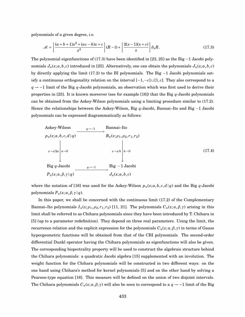
polynomials of a given degree, i.e.
M =[
(a+b+1)x2 + (ac−b)x+ cx2
](R− I)+
[2(x−1)(x+ c)
x
]∂xR. (17.3)
The polynomial eigenfunctions of (17.3) have been identified in [23, 25] as the Big −1 Jacobi poly-
nomials Jn(x;a,b, c) introduced in [25]. Alternatively, one can obtain the polynomials Jn(x;a,b, c)
by directly applying the limit (17.2) to the BI polynomials. The Big −1 Jacobi polynomials sat-
isfy a continuous orthogonality relation on the interval [−1,−c]∪ [1, c]. They also correspond to a
q →−1 limit of the Big q-Jacobi polynomials, an observation which was first used to derive their
properties in [25]. It is known moreover (see for example [16]) that the Big q-Jacobi polynomials
can be obtained from the Askey-Wilson polynomials using a limiting procedure similar to (17.2).
Hence the relationships between the Askey-Wilson, Big q-Jacobi, Bannai–Ito and Big −1 Jacobi
polynomials can be expressed diagrammatically as follows:
Askey-Wilson
pn(x;a,b, c,d |q)
q→−1//
a→0x→x/2a
Bannai–Ito
Bn(x;ρ1,ρ2, r1, r2)
h→0x→x/h
Big q-Jacobi
Pn(x;α,β,γ |q)
q→−1//Big −1 Jacobi
Jn(x;a,b, c)
(17.4)
where the notation of [16] was used for the Askey-Wilson pn(x;a,b, c,d |q) and the Big q-Jacobi
polynomials Pn(x;α,β,γ |q).
In this paper, we shall be concerned with the continuous limit (17.2) of the Complementary
Bannai–Ito polynomials In(x;ρ1,ρ2, r1, r2) [11, 21]. The polynomials Cn(x;α,β,γ) arising in this
limit shall be referred to as Chihara polynomials since they have been introduced by T. Chihara in
[5] (up to a parameter redefinition). They depend on three real parameters. Using the limit, the
recurrence relation and the explicit expression for the polynomials Cn(x;α,β,γ) in terms of Gauss
hypergeometric functions will be obtained from that of the CBI polynomials. The second-order
differential Dunkl operator having the Chihara polynomials as eigenfunctions will also be given.
The corresponding bispectrality property will be used to construct the algebraic structure behind
the Chihara polynomials: a quadratic Jacobi algebra [15] supplemented with an involution. The
weight function for the Chihara polynomials will be constructed in two different ways: on the
one hand using Chihara’s method for kernel polynomials [5] and on the other hand by solving a
Pearson-type equation [16]. This measure will be defined on the union of two disjoint intervals.
The Chihara polynomials Cn(x;α,β,γ) will also be seen to correspond to a q →−1 limit of the Big
433
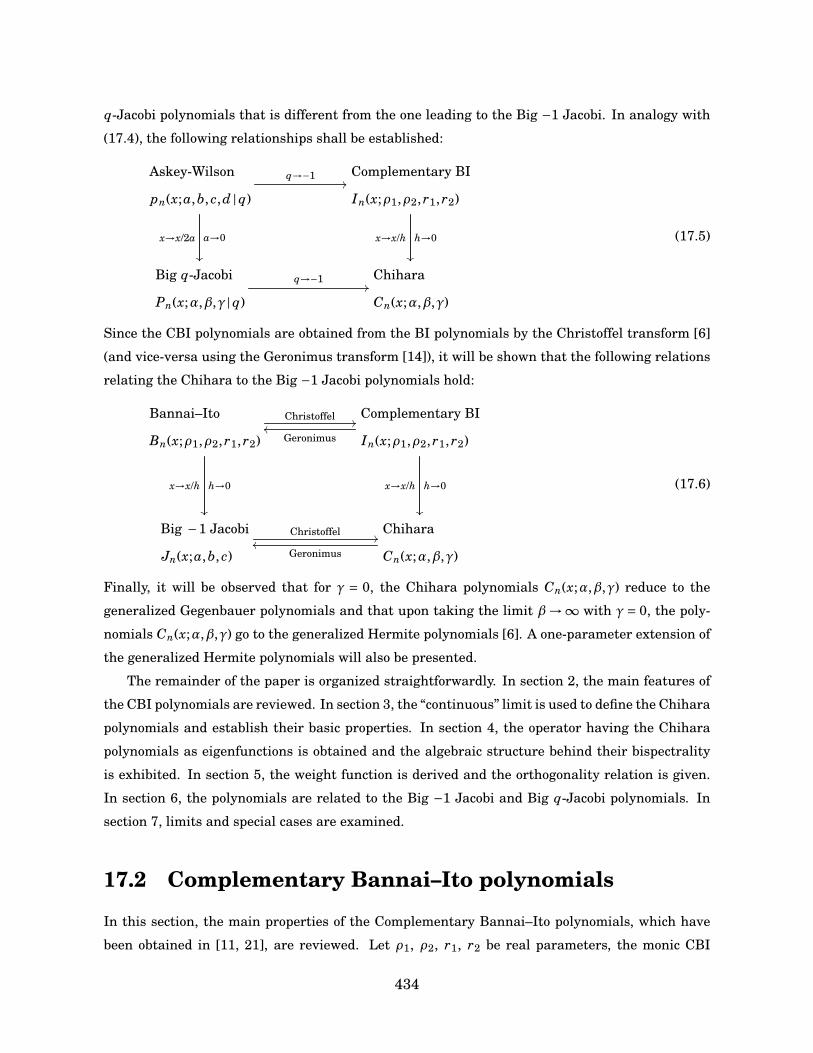
q-Jacobi polynomials that is different from the one leading to the Big −1 Jacobi. In analogy with
(17.4), the following relationships shall be established:
Askey-Wilson
pn(x;a,b, c,d |q)
q→−1//
a→0x→x/2a
Complementary BI
In(x;ρ1,ρ2, r1, r2)
h→0x→x/h
Big q-Jacobi
Pn(x;α,β,γ |q)
q→−1//Chihara
Cn(x;α,β,γ)
(17.5)
Since the CBI polynomials are obtained from the BI polynomials by the Christoffel transform [6]
(and vice-versa using the Geronimus transform [14]), it will be shown that the following relations
relating the Chihara to the Big −1 Jacobi polynomials hold:
Bannai–Ito
Bn(x;ρ1,ρ2, r1, r2)
Christoffel //
h→0x→x/h
Complementary BI
In(x;ρ1,ρ2, r1, r2)Geronimusoo
h→0x→x/h
Big −1 Jacobi
Jn(x;a,b, c)
Christoffel //Chihara
Cn(x;α,β,γ)Geronimusoo
(17.6)
Finally, it will be observed that for γ = 0, the Chihara polynomials Cn(x;α,β,γ) reduce to the
generalized Gegenbauer polynomials and that upon taking the limit β→∞ with γ = 0, the poly-
nomials Cn(x;α,β,γ) go to the generalized Hermite polynomials [6]. A one-parameter extension of
the generalized Hermite polynomials will also be presented.
The remainder of the paper is organized straightforwardly. In section 2, the main features of
the CBI polynomials are reviewed. In section 3, the “continuous” limit is used to define the Chihara
polynomials and establish their basic properties. In section 4, the operator having the Chihara
polynomials as eigenfunctions is obtained and the algebraic structure behind their bispectrality
is exhibited. In section 5, the weight function is derived and the orthogonality relation is given.
In section 6, the polynomials are related to the Big −1 Jacobi and Big q-Jacobi polynomials. In
section 7, limits and special cases are examined.
17.2 Complementary Bannai–Ito polynomials
In this section, the main properties of the Complementary Bannai–Ito polynomials, which have
been obtained in [11, 21], are reviewed. Let ρ1, ρ2, r1, r2 be real parameters, the monic CBI
434
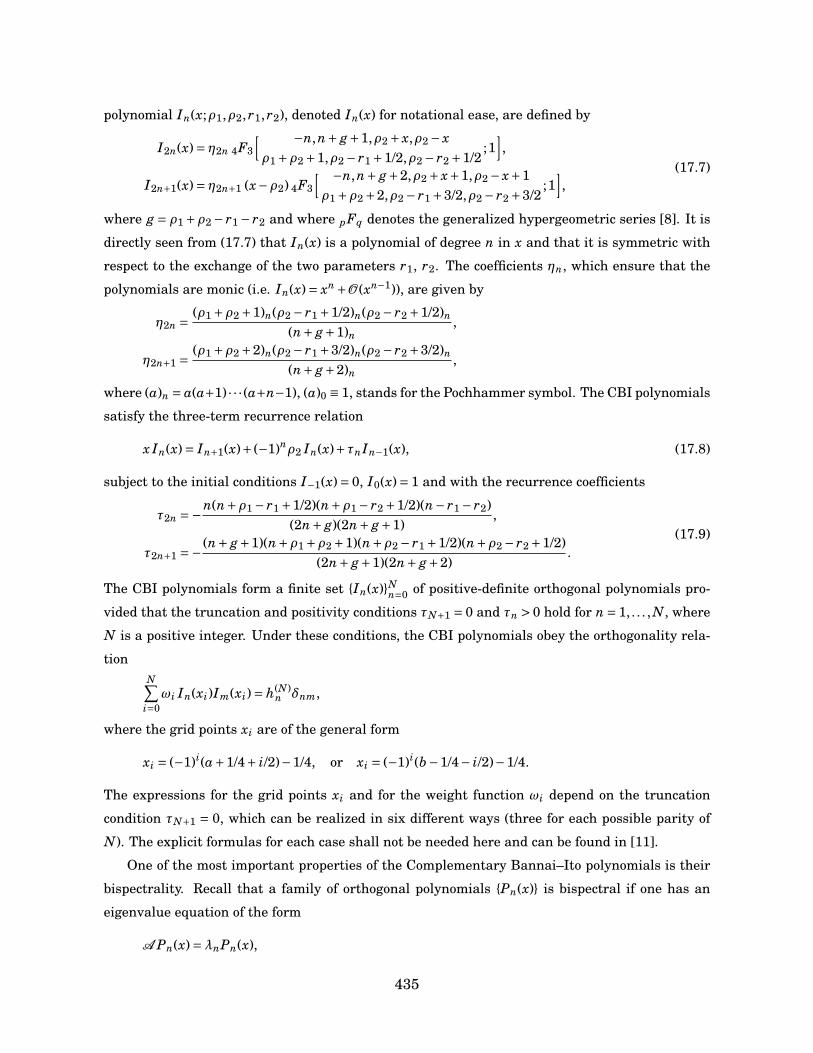
polynomial In(x;ρ1,ρ2, r1, r2), denoted In(x) for notational ease, are defined by
I2n(x)= η2n 4F3
[ −n,n+ g+1,ρ2 + x,ρ2 − xρ1 +ρ2 +1,ρ2 − r1 +1/2,ρ2 − r2 +1/2
;1],
I2n+1(x)= η2n+1 (x−ρ2) 4F3
[ −n,n+ g+2,ρ2 + x+1,ρ2 − x+1ρ1 +ρ2 +2,ρ2 − r1 +3/2,ρ2 − r2 +3/2
;1],
(17.7)
where g = ρ1 +ρ2 − r1 − r2 and where pFq denotes the generalized hypergeometric series [8]. It is
directly seen from (17.7) that In(x) is a polynomial of degree n in x and that it is symmetric with
respect to the exchange of the two parameters r1, r2. The coefficients ηn, which ensure that the
polynomials are monic (i.e. In(x)= xn +O (xn−1)), are given by
η2n = (ρ1 +ρ2 +1)n(ρ2 − r1 +1/2)n(ρ2 − r2 +1/2)n
(n+ g+1)n,
η2n+1 = (ρ1 +ρ2 +2)n(ρ2 − r1 +3/2)n(ρ2 − r2 +3/2)n
(n+ g+2)n,
where (a)n = a(a+1) · · · (a+n−1), (a)0 ≡ 1, stands for the Pochhammer symbol. The CBI polynomials
satisfy the three-term recurrence relation
x In(x)= In+1(x)+ (−1)nρ2 In(x)+τnIn−1(x), (17.8)
subject to the initial conditions I−1(x)= 0, I0(x)= 1 and with the recurrence coefficients
τ2n =−n(n+ρ1 − r1 +1/2)(n+ρ1 − r2 +1/2)(n− r1 − r2)(2n+ g)(2n+ g+1)
,
τ2n+1 =− (n+ g+1)(n+ρ1 +ρ2 +1)(n+ρ2 − r1 +1/2)(n+ρ2 − r2 +1/2)(2n+ g+1)(2n+ g+2)
.(17.9)
The CBI polynomials form a finite set In(x)Nn=0 of positive-definite orthogonal polynomials pro-
vided that the truncation and positivity conditions τN+1 = 0 and τn > 0 hold for n = 1, . . . , N, where
N is a positive integer. Under these conditions, the CBI polynomials obey the orthogonality rela-
tionN∑
i=0ωi In(xi)Im(xi)= h(N)
n δnm,
where the grid points xi are of the general form
xi = (−1)i(a+1/4+ i/2)−1/4, or xi = (−1)i(b−1/4− i/2)−1/4.
The expressions for the grid points xi and for the weight function ωi depend on the truncation
condition τN+1 = 0, which can be realized in six different ways (three for each possible parity of
N). The explicit formulas for each case shall not be needed here and can be found in [11].
One of the most important properties of the Complementary Bannai–Ito polynomials is their
bispectrality. Recall that a family of orthogonal polynomials Pn(x) is bispectral if one has an
eigenvalue equation of the form
A Pn(x)=λnPn(x),
435
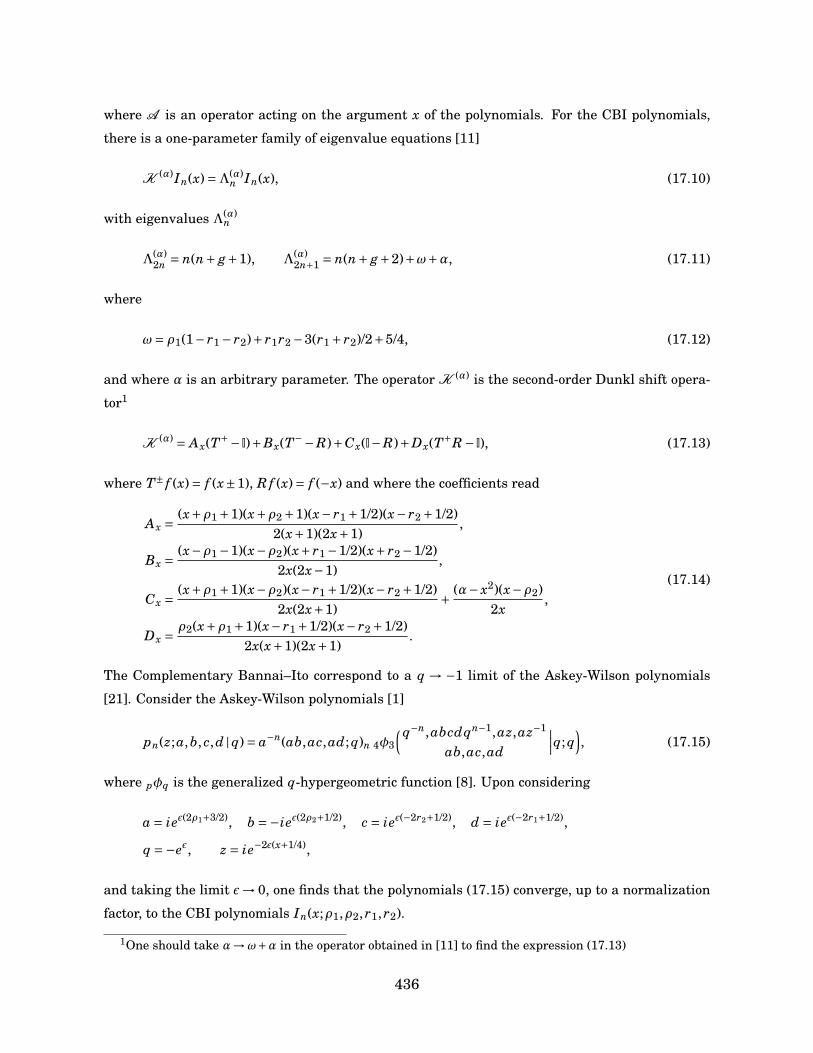
where A is an operator acting on the argument x of the polynomials. For the CBI polynomials,
there is a one-parameter family of eigenvalue equations [11]
K (α)In(x)=Λ(α)n In(x), (17.10)
with eigenvalues Λ(α)n
Λ(α)2n = n(n+ g+1), Λ(α)
2n+1 = n(n+ g+2)+ω+α, (17.11)
where
ω= ρ1(1− r1 − r2)+ r1r2 −3(r1 + r2)/2+5/4, (17.12)
and where α is an arbitrary parameter. The operator K (α) is the second-order Dunkl shift opera-
tor1
K (α) = Ax(T+− I)+Bx(T−−R)+Cx(I−R)+Dx(T+R− I), (17.13)
where T± f (x)= f (x±1), R f (x)= f (−x) and where the coefficients read
Ax = (x+ρ1 +1)(x+ρ2 +1)(x− r1 +1/2)(x− r2 +1/2)2(x+1)(2x+1)
,
Bx = (x−ρ1 −1)(x−ρ2)(x+ r1 −1/2)(x+ r2 −1/2)2x(2x−1)
,
Cx = (x+ρ1 +1)(x−ρ2)(x− r1 +1/2)(x− r2 +1/2)2x(2x+1)
+ (α− x2)(x−ρ2)2x
,
Dx = ρ2(x+ρ1 +1)(x− r1 +1/2)(x− r2 +1/2)2x(x+1)(2x+1)
.
(17.14)
The Complementary Bannai–Ito correspond to a q → −1 limit of the Askey-Wilson polynomials
[21]. Consider the Askey-Wilson polynomials [1]
pn(z;a,b, c,d |q)= a−n(ab,ac,ad; q)n 4φ3
( q−n,abcdqn−1,az,az−1
ab,ac,ad
∣∣∣q; q), (17.15)
where pφq is the generalized q-hypergeometric function [8]. Upon considering
a = ieε(2ρ1+3/2), b =−ieε(2ρ2+1/2), c = ieε(−2r2+1/2), d = ieε(−2r1+1/2),
q =−eε, z = ie−2ε(x+1/4),
and taking the limit ε→ 0, one finds that the polynomials (17.15) converge, up to a normalization
factor, to the CBI polynomials In(x;ρ1,ρ2, r1, r2).
1One should take α→ω+α in the operator obtained in [11] to find the expression (17.13)
436
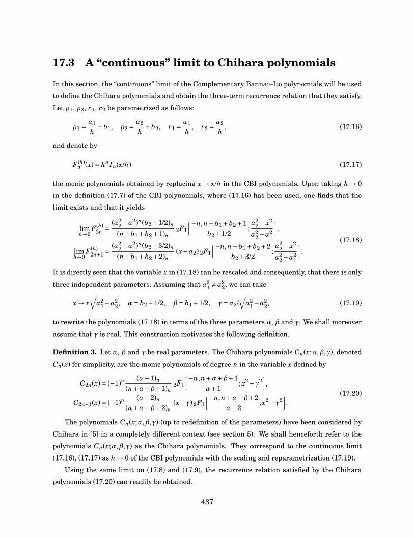
17.3 A “continuous” limit to Chihara polynomials
In this section, the “continuous” limit of the Complementary Bannai–Ito polynomials will be used
to define the Chihara polynomials and obtain the three-term recurrence relation that they satisfy.
Let ρ1, ρ2, r1, r2 be parametrized as follows:
ρ1 = a1
h+b1, ρ2 = a2
h+b2, r1 = a1
h, r2 = a2
h, (17.16)
and denote by
F (h)n (x)= hnIn(x/h) (17.17)
the monic polynomials obtained by replacing x → x/h in the CBI polynomials. Upon taking h → 0
in the definition (17.7) of the CBI polynomials, where (17.16) has been used, one finds that the
limit exists and that it yields
limh→0
F (h)2n = (a2
2 −a21)n(b2 +1/2)n
(n+b1 +b2 +1)n2F1
[−n,n+b1 +b2 +1b2 +1/2
;a2
2 − x2
a22 −a2
1
],
limh→0
F (h)2n+1 =
(a22 −a2
1)n(b2 +3/2)n
(n+b1 +b2 +2)n(x−a2) 2F1
[−n,n+b1 +b2 +2b2 +3/2
;a2
2 − x2
a22 −a2
1
].
(17.18)
It is directly seen that the variable x in (17.18) can be rescaled and consequently, that there is only
three independent parameters. Assuming that a21 6= a2
2, we can take
x → x√
a21 −a2
2, α= b2 −1/2, β= b1 +1/2, γ= a2/√
a21 −a2
2, (17.19)
to rewrite the polynomials (17.18) in terms of the three parameters α, β and γ. We shall moreover
assume that γ is real. This construction motivates the following definition.
Definition 3. Let α, β and γ be real parameters. The Chihara polynomials Cn(x;α,β,γ), denoted
Cn(x) for simplicity, are the monic polynomials of degree n in the variable x defined by
C2n(x)= (−1)n (α+1)n
(n+α+β+1)n2F1
[−n,n+α+β+1α+1
; x2 −γ2],
C2n+1(x)= (−1)n (α+2)n
(n+α+β+2)n(x−γ) 2F1
[−n,n+α+β+2α+2
; x2 −γ2].
(17.20)
The polynomials Cn(x;α,β,γ) (up to redefinition of the parameters) have been considered by
Chihara in [5] in a completely different context (see section 5). We shall henceforth refer to the
polynomials Cn(x;α,β,γ) as the Chihara polynomials. They correspond to the continuous limit
(17.16), (17.17) as h → 0 of the CBI polynomials with the scaling and reparametrization (17.19).
Using the same limit on (17.8) and (17.9), the recurrence relation satisfied by the Chihara
polynomials (17.20) can readily be obtained.
437
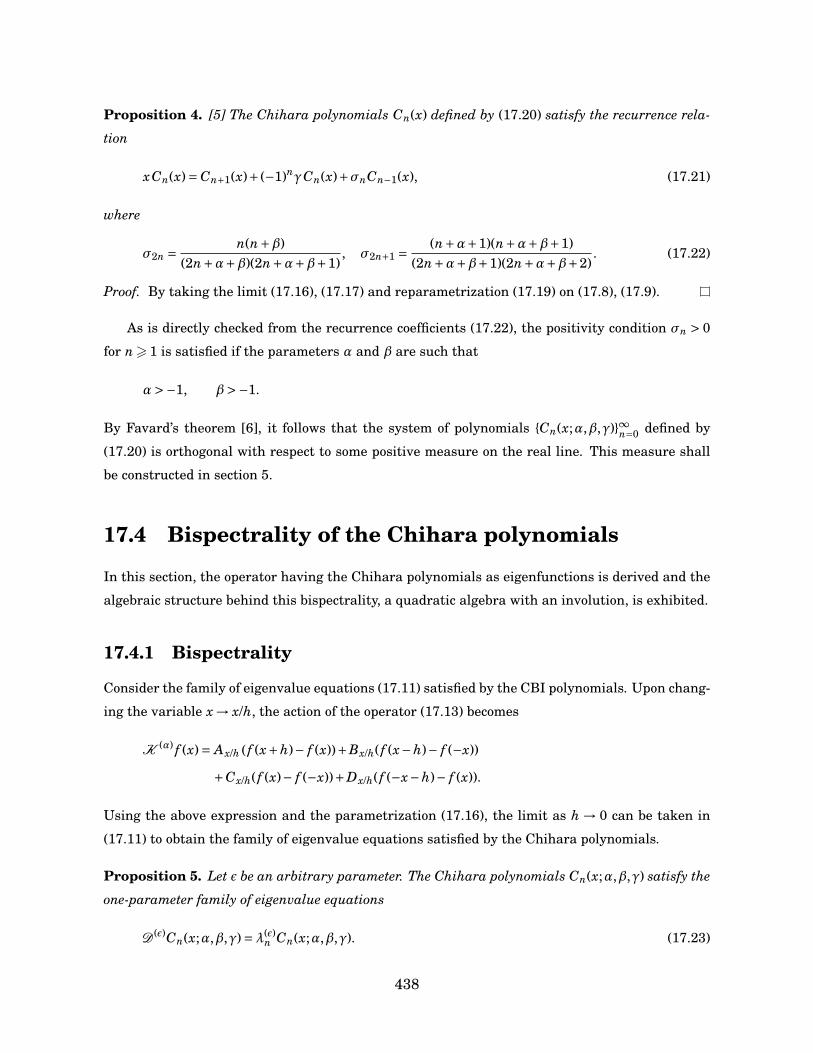
Proposition 4. [5] The Chihara polynomials Cn(x) defined by (17.20) satisfy the recurrence rela-
tion
xCn(x)= Cn+1(x)+ (−1)nγCn(x)+σnCn−1(x), (17.21)
where
σ2n = n(n+β)(2n+α+β)(2n+α+β+1)
, σ2n+1 = (n+α+1)(n+α+β+1)(2n+α+β+1)(2n+α+β+2)
. (17.22)
Proof. By taking the limit (17.16), (17.17) and reparametrization (17.19) on (17.8), (17.9).
As is directly checked from the recurrence coefficients (17.22), the positivity condition σn > 0
for n> 1 is satisfied if the parameters α and β are such that
α>−1, β>−1.
By Favard’s theorem [6], it follows that the system of polynomials Cn(x;α,β,γ)∞n=0 defined by
(17.20) is orthogonal with respect to some positive measure on the real line. This measure shall
be constructed in section 5.
17.4 Bispectrality of the Chihara polynomials
In this section, the operator having the Chihara polynomials as eigenfunctions is derived and the
algebraic structure behind this bispectrality, a quadratic algebra with an involution, is exhibited.
17.4.1 Bispectrality
Consider the family of eigenvalue equations (17.11) satisfied by the CBI polynomials. Upon chang-
ing the variable x → x/h, the action of the operator (17.13) becomes
K (α) f (x)= Ax/h ( f (x+h)− f (x))+Bx/h( f (x−h)− f (−x))
+Cx/h( f (x)− f (−x))+Dx/h( f (−x−h)− f (x)).
Using the above expression and the parametrization (17.16), the limit as h → 0 can be taken in
(17.11) to obtain the family of eigenvalue equations satisfied by the Chihara polynomials.
Proposition 5. Let ε be an arbitrary parameter. The Chihara polynomials Cn(x;α,β,γ) satisfy the
one-parameter family of eigenvalue equations
D(ε)Cn(x;α,β,γ)=λ(ε)n Cn(x;α,β,γ). (17.23)
438
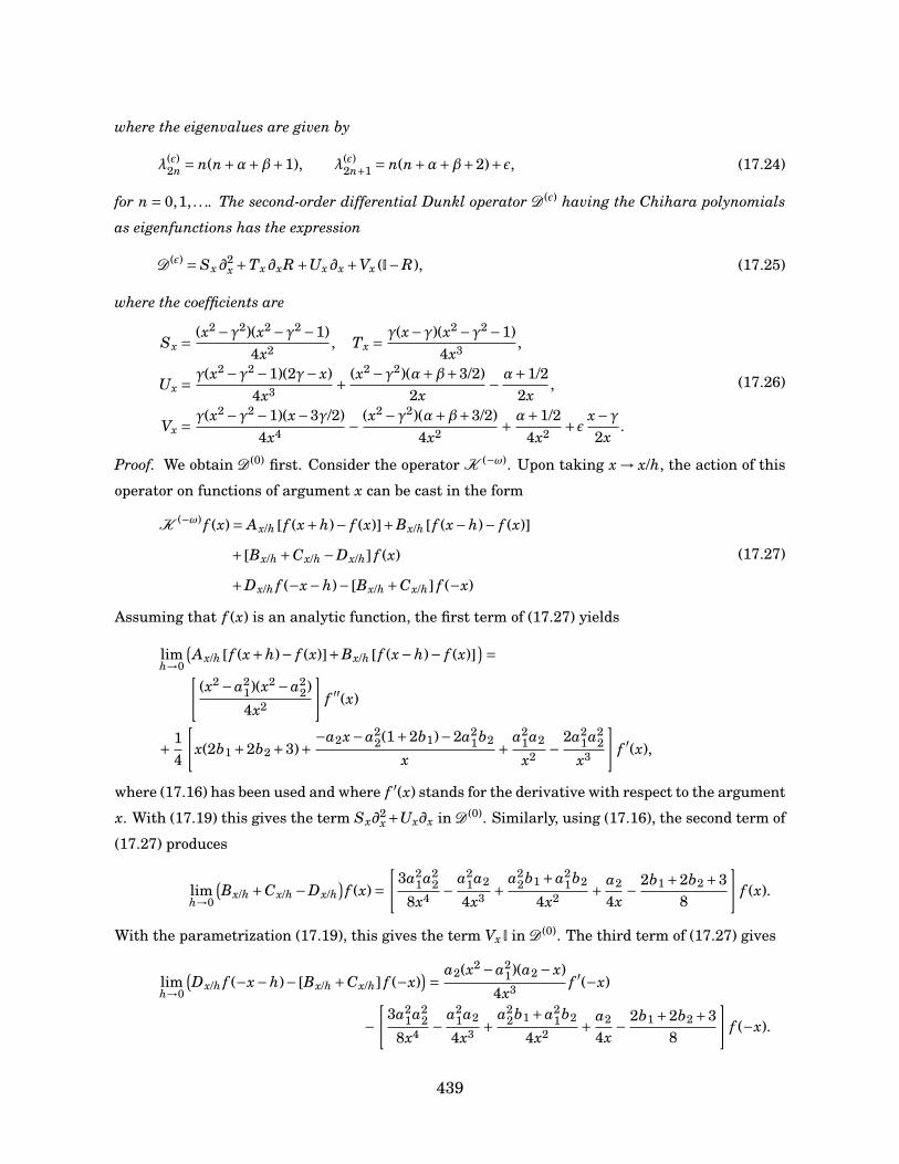
where the eigenvalues are given by
λ(ε)2n = n(n+α+β+1), λ(ε)
2n+1 = n(n+α+β+2)+ε, (17.24)
for n = 0,1, . . .. The second-order differential Dunkl operator D(ε) having the Chihara polynomials
as eigenfunctions has the expression
D(ε) = Sx ∂2x +Tx ∂xR+Ux ∂x +Vx (I−R), (17.25)
where the coefficients are
Sx = (x2 −γ2)(x2 −γ2 −1)4x2 , Tx = γ(x−γ)(x2 −γ2 −1)
4x3 ,
Ux = γ(x2 −γ2 −1)(2γ− x)4x3 + (x2 −γ2)(α+β+3/2)
2x− α+1/2
2x,
Vx = γ(x2 −γ2 −1)(x−3γ/2)4x4 − (x2 −γ2)(α+β+3/2)
4x2 + α+1/24x2 +ε x−γ
2x.
(17.26)
Proof. We obtain D(0) first. Consider the operator K (−ω). Upon taking x → x/h, the action of this
operator on functions of argument x can be cast in the form
K (−ω) f (x)= Ax/h [ f (x+h)− f (x)]+Bx/h [ f (x−h)− f (x)]
+ [Bx/h +Cx/h −Dx/h] f (x)
+Dx/h f (−x−h)− [Bx/h +Cx/h] f (−x)
(17.27)
Assuming that f (x) is an analytic function, the first term of (17.27) yields
limh→0
(Ax/h [ f (x+h)− f (x)]+Bx/h [ f (x−h)− f (x)]
)=[(x2 −a2
1)(x2 −a22)
4x2
]f ′′(x)
+ 14
[x(2b1 +2b2 +3)+ −a2x−a2
2(1+2b1)−2a21b2
x+ a2
1a2
x2 − 2a21a2
2
x3
]f ′(x),
where (17.16) has been used and where f ′(x) stands for the derivative with respect to the argument
x. With (17.19) this gives the term Sx∂2x+Ux∂x in D(0). Similarly, using (17.16), the second term of
(17.27) produces
limh→0
(Bx/h +Cx/h −Dx/h
)f (x)=
[3a2
1a22
8x4 − a21a2
4x3 + a22b1 +a2
1b2
4x2 + a2
4x− 2b1 +2b2 +3
8
]f (x).
With the parametrization (17.19), this gives the term Vx I in D(0). The third term of (17.27) gives
limh→0
(Dx/h f (−x−h)− [Bx/h +Cx/h] f (−x)
)= a2(x2 −a21)(a2 − x)
4x3 f ′(−x)
−[
3a21a2
2
8x4 − a21a2
4x3 + a22b1 +a2
1b2
4x2 + a2
4x− 2b1 +2b2 +3
8
]f (−x).
439

Using (17.19), this gives the term −Vx R+Tx ∂xR in D(0). The arbitrary parameter ε can be added
to the odd part of the spectrum since the Chihara polynomials satisfy the eigenvalue equation
(x−γ)2x
(I−R)Cn(x)= ρnCn(x), with ρn =
0 if n is even,
1 if n is odd,
as can be seen directly from the explicit expression (17.20). This concludes the proof.
17.4.2 Algebraic Structure
The bispectrality property of the Chihara polynomials can be encoded algebraically. Let κ1, κ2 and
P be defined as follows
κ1 =D(ε), κ2 = x, P = R+ γ
x(I−R),
where D(ε) is given by (17.25), R is the reflection operator and where κ2 corresponds to multiplica-
tion by x. It is directly checked that P is an involution, which means that
P2 = I.
Upon defining a third generator
κ3 = [κ1,κ2],
with [a,b]= ab−ba, a direct computation shows that one has the commutation relations
[κ3,κ2]= 12κ2
2 +δ2κ22P +2δ3κ3P −δ5P −δ4,
[κ1,κ3]= 12
κ1,κ2−δ2κ3P −δ3κ1P +δ1κ2 −δ1δ3P,(17.28)
where a,b = ab+ ba stands for the anticommutator. The commutation relations involving the
involution P are given by
[κ1,P]= 0, κ2,P= 2δ3, κ3,P= 0, (17.29)
and the structure constants δi, i = 1, . . . ,5 are expressed as follows:
δ1 = ε(α+β+1−ε), δ2 = (α+β+3/2−2ε), δ3 = γ,
δ4 = (γ2 +1)/2, δ5 = γ2(α+β+3/2−2ε)+α+1/2.
The algebra defined by (17.28) and (17.29) corresponds to a Jacobi algebra [15] supplemented with
involutions and can be seen as a contraction of the Complementary Bannai–Ito algebra [11].
440
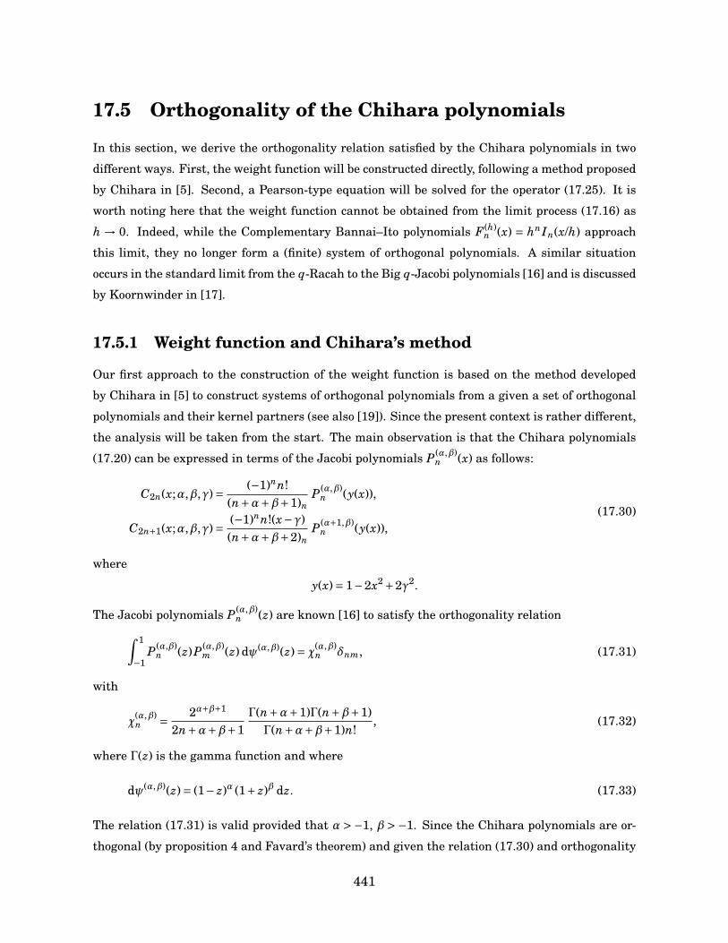
17.5 Orthogonality of the Chihara polynomials
In this section, we derive the orthogonality relation satisfied by the Chihara polynomials in two
different ways. First, the weight function will be constructed directly, following a method proposed
by Chihara in [5]. Second, a Pearson-type equation will be solved for the operator (17.25). It is
worth noting here that the weight function cannot be obtained from the limit process (17.16) as
h → 0. Indeed, while the Complementary Bannai–Ito polynomials F (h)n (x) = hnIn(x/h) approach
this limit, they no longer form a (finite) system of orthogonal polynomials. A similar situation
occurs in the standard limit from the q-Racah to the Big q-Jacobi polynomials [16] and is discussed
by Koornwinder in [17].
17.5.1 Weight function and Chihara’s method
Our first approach to the construction of the weight function is based on the method developed
by Chihara in [5] to construct systems of orthogonal polynomials from a given a set of orthogonal
polynomials and their kernel partners (see also [19]). Since the present context is rather different,
the analysis will be taken from the start. The main observation is that the Chihara polynomials
(17.20) can be expressed in terms of the Jacobi polynomials P(α,β)n (x) as follows:
C2n(x;α,β,γ)= (−1)nn!(n+α+β+1)n
P(α,β)n (y(x)),
C2n+1(x;α,β,γ)= (−1)nn!(x−γ)(n+α+β+2)n
P(α+1,β)n (y(x)),
(17.30)
where
y(x)= 1−2x2 +2γ2.
The Jacobi polynomials P(α,β)n (z) are known [16] to satisfy the orthogonality relation∫ 1
−1P(α,β)
n (z)P(α,β)m (z) dψ(α,β)(z)= χ(α,β)
n δnm, (17.31)
with
χ(α,β)n = 2α+β+1
2n+α+β+1Γ(n+α+1)Γ(n+β+1)Γ(n+α+β+1)n!
, (17.32)
where Γ(z) is the gamma function and where
dψ(α,β)(z)= (1− z)α (1+ z)β dz. (17.33)
The relation (17.31) is valid provided that α>−1, β>−1. Since the Chihara polynomials are or-
thogonal (by proposition 4 and Favard’s theorem) and given the relation (17.30) and orthogonality
441

relation (17.31), we consider the integral
IMN =∫F
CM(x)CN (x) dφ(x),
where the interval F = [−√
1+γ2,−|γ| ] ∪ [ |γ|,√
1+γ2] corresponds to the inverse mapping of the
interval [−1,1] for y(x) and where φ(x) is a distribution function. Upon taking M = 2m and using
(17.30), one directly has (up to normalization)
I2m,2n =∫ p
1+γ2
|γ|P(α,β)
m(y(x)
)P(α,β)
n(y(x)
) [dφ(x)−dφ(−x)
],
I2m,2n+1 =∫ p
1+γ2
|γ|P(α,β)
m(y(x)
)P(α+1,β)
n(y(x)
) [(x−γ)dφ(x)+ (x+γ)dφ(−x)
].
In order that I2n,2m =I2n,2m+1 = 0 for n 6= m, one must have for |γ|6 x6√
1+γ2
dφ(x)−dφ(−x)= dψ(α,β)(y(x)),
(x−γ)dφ(x)+ (x+γ)dφ(−x)= 0,(17.34)
where ψ(α,β)(y(x))
is the distribution appearing in (17.33) with z = y(x). The common solution to
the equations (17.34) is seen to be given by
dφ(x)= (x+γ)2|x| dψ(α,β)(1−2x2 +2γ2). (17.35)
It is easily verified that the condition I2n+1,2m+1 = 0 for n 6= m holds. Indeed, upon using (17.35)
one finds (up to normalization)
I2n+1,2m+1 =∫ p
1+γ2
|γ|P(α+1,β)
n(y(x)
)P(α+1,β)
m(y(x)
) [(x−γ)2 dφ(x)− (x+γ)2 dφ(−x)
]=
∫ p1+γ2
|γ|P(α+1,β)
n(y(x)
)P(α+1,β)
m(y(x)
)dψ(α+1,β)(y(x)
)= χ(α+1,β)n δnm,
which follows from (17.31). The following result has thus been established.
Proposition 6. [5] Let α, β and γ be real parameters such that α,β>−1. The Chihara polynomials
Cn(x;α,β,γ) satisfy the orthogonality relation∫E
Cn(x)Cm(x)ω(x) dx = knδnm, (17.36)
on the interval E = [−√
1+γ2,−|γ| ] ∪ [ |γ|,√
1+γ2 ]. The weight function has the expression
ω(x)= θ(x) (x+γ) (x2 −γ2)α (1+γ2 − x2)β, (17.37)
where θ(x) is the sign function. The normalization factor kn is given by
k2n = Γ(n+α+1)Γ(n+β+1)Γ(n+α+β+1)
n!
(2n+α+β+1)[(n+α+β+1)n
]2 ,
k2n+1 = Γ(n+α+2)Γ(n+β+1)Γ(n+α+β+2)
n!
(2n+α+β+2)[(n+α+β+2)n
]2
(17.38)
442
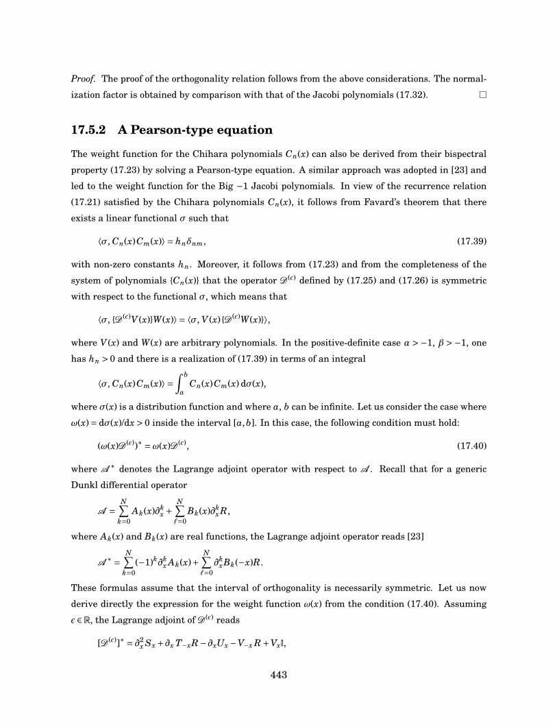
Proof. The proof of the orthogonality relation follows from the above considerations. The normal-
ization factor is obtained by comparison with that of the Jacobi polynomials (17.32).
17.5.2 A Pearson-type equation
The weight function for the Chihara polynomials Cn(x) can also be derived from their bispectral
property (17.23) by solving a Pearson-type equation. A similar approach was adopted in [23] and
led to the weight function for the Big −1 Jacobi polynomials. In view of the recurrence relation
(17.21) satisfied by the Chihara polynomials Cn(x), it follows from Favard’s theorem that there
exists a linear functional σ such that
⟨σ, Cn(x)Cm(x)⟩ = hnδnm, (17.39)
with non-zero constants hn. Moreover, it follows from (17.23) and from the completeness of the
system of polynomials Cn(x) that the operator D(ε) defined by (17.25) and (17.26) is symmetric
with respect to the functional σ, which means that
⟨σ, D(ε)V (x)W(x)⟩ = ⟨σ, V (x) D(ε)W(x)⟩,
where V (x) and W(x) are arbitrary polynomials. In the positive-definite case α > −1, β > −1, one
has hn > 0 and there is a realization of (17.39) in terms of an integral
⟨σ, Cn(x)Cm(x)⟩ =∫ b
aCn(x)Cm(x) dσ(x),
where σ(x) is a distribution function and where a, b can be infinite. Let us consider the case where
ω(x)= dσ(x)/dx > 0 inside the interval [a,b]. In this case, the following condition must hold:
(ω(x)D(ε))∗ =ω(x)D(ε), (17.40)
where A ∗ denotes the Lagrange adjoint operator with respect to A . Recall that for a generic
Dunkl differential operator
A =N∑
k=0Ak(x)∂k
x +N∑`=0
Bk(x)∂kxR,
where Ak(x) and Bk(x) are real functions, the Lagrange adjoint operator reads [23]
A ∗ =N∑
k=0(−1)k∂k
x Ak(x)+N∑`=0
∂kxBk(−x)R.
These formulas assume that the interval of orthogonality is necessarily symmetric. Let us now
derive directly the expression for the weight function ω(x) from the condition (17.40). Assuming
ε ∈R, the Lagrange adjoint of D(ε) reads
[D(ε)]∗ = ∂2x Sx +∂x T−xR−∂xUx −V−x R+VxI,
443
where the coefficients are given by (17.26). Upon imposing the condition (17.40), one finds the
following equations for the terms in ∂xR and ∂x:
(x+γ)ω(−x)+ (−x+γ)ω(x)= 0,
ω′(x)=[
α
x−γ + α+1x+γ − 2xβ
γ2 +1− x2
]ω(x).
(17.41)
It is easily seen that the common solution to (17.41) is given by
ω(x)= θ(x) (x+γ) (x2 −γ2)α (1+γ2 − x2)β, (17.42)
which corresponds to the weight function (17.37) derived above. It is directly checked that with
(17.42), the equations for the terms in ∂2x, R and I arising from the symmetry condition (17.40) are
identically satisfied. The orthogonality relation (17.36) can be recovered by the requirements that
ω(x)> 0 on a symmetric interval.
17.6 Chihara polynomials and
Big q and −1 Jacobi polynomials
In this section, the connexion between the Chihara polynomials and the Big q-Jacobi and Big −1
Jacobi polynomials is established. In particular, it is shown that the Chihara polynomials are
related to the former by a q →−1 limit and to the latter by a Christoffel transformation.
17.6.1 Chihara polynomials and Big −1 Jacobi polynomials
The Big −1 Jacobi polynomials Jn(x;a,b, c) were introduced in [25] as a q →−1 limit of the Big q-
Jacobi polynomials. In [23], they were seen to be the polynomials that diagonalize the most general
first order differential Dunkl operator preserving the space of polynomials of a given degree (see
(17.3)). The Big −1 Jacobi polynomials can be defined by their recurrence relation
x Jn(x)= Jn+1(x)+ (1− An −Cn)Jn(x)+ An−1CnJn−1, (17.43)
subject to the initial conditions J−1(x)= 0, J0(x)= 1 and where the recurrence coefficients read
An =
(1+c)(a+n+1)
2n+a+b+2 neven
(1−c)(n+a+b+1)2n+a+b+2 nodd
, Cn =
(1−c)n
2n+a+b neven
(1+c)(n+b)2n+a+b nodd
, (17.44)
for 0 < c < 1. Consider the monic polynomials Kn(x) obtained from the Big −1 Jacobi polynomials
Jn(x) by the Christoffel transformation [6]
Kn(x)= 1(x−1)
[Jn+1(x)− Jn+1(1)
Jn(1)Jn(x)
]= (x−1)−1[Jn+1(x)− AnJn(x)], (17.45)
444
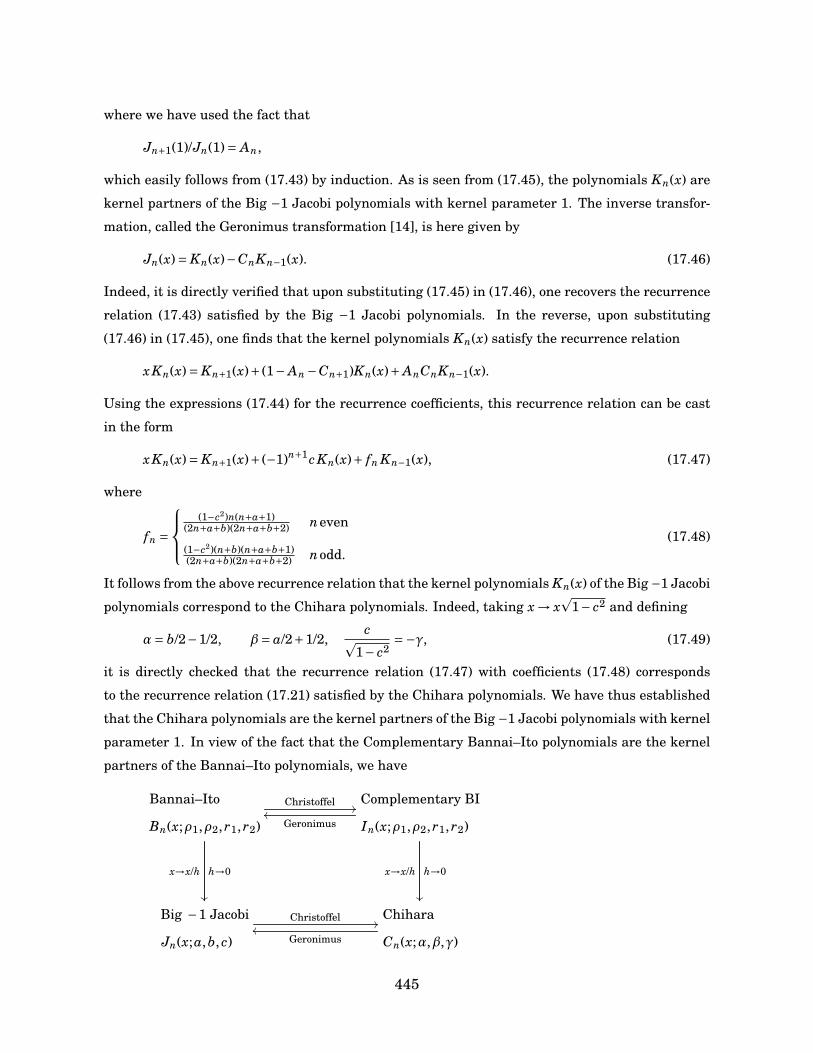
where we have used the fact that
Jn+1(1)/Jn(1)= An,
which easily follows from (17.43) by induction. As is seen from (17.45), the polynomials Kn(x) are
kernel partners of the Big −1 Jacobi polynomials with kernel parameter 1. The inverse transfor-
mation, called the Geronimus transformation [14], is here given by
Jn(x)= Kn(x)−CnKn−1(x). (17.46)
Indeed, it is directly verified that upon substituting (17.45) in (17.46), one recovers the recurrence
relation (17.43) satisfied by the Big −1 Jacobi polynomials. In the reverse, upon substituting
(17.46) in (17.45), one finds that the kernel polynomials Kn(x) satisfy the recurrence relation
xKn(x)= Kn+1(x)+ (1− An −Cn+1)Kn(x)+ AnCnKn−1(x).
Using the expressions (17.44) for the recurrence coefficients, this recurrence relation can be cast
in the form
xKn(x)= Kn+1(x)+ (−1)n+1c Kn(x)+ fn Kn−1(x), (17.47)
where
fn =
(1−c2)n(n+a+1)
(2n+a+b)(2n+a+b+2) neven
(1−c2)(n+b)(n+a+b+1)(2n+a+b)(2n+a+b+2) nodd.
(17.48)
It follows from the above recurrence relation that the kernel polynomials Kn(x) of the Big −1 Jacobi
polynomials correspond to the Chihara polynomials. Indeed, taking x → xp
1− c2 and defining
α= b/2−1/2, β= a/2+1/2,cp
1− c2=−γ, (17.49)
it is directly checked that the recurrence relation (17.47) with coefficients (17.48) corresponds
to the recurrence relation (17.21) satisfied by the Chihara polynomials. We have thus established
that the Chihara polynomials are the kernel partners of the Big −1 Jacobi polynomials with kernel
parameter 1. In view of the fact that the Complementary Bannai–Ito polynomials are the kernel
partners of the Bannai–Ito polynomials, we have
Bannai–Ito
Bn(x;ρ1,ρ2, r1, r2)
Christoffel //
h→0x→x/h
Complementary BI
In(x;ρ1,ρ2, r1, r2)Geronimusoo
h→0x→x/h
Big −1 Jacobi
Jn(x;a,b, c)
Christoffel //Chihara
Cn(x;α,β,γ)Geronimusoo
445
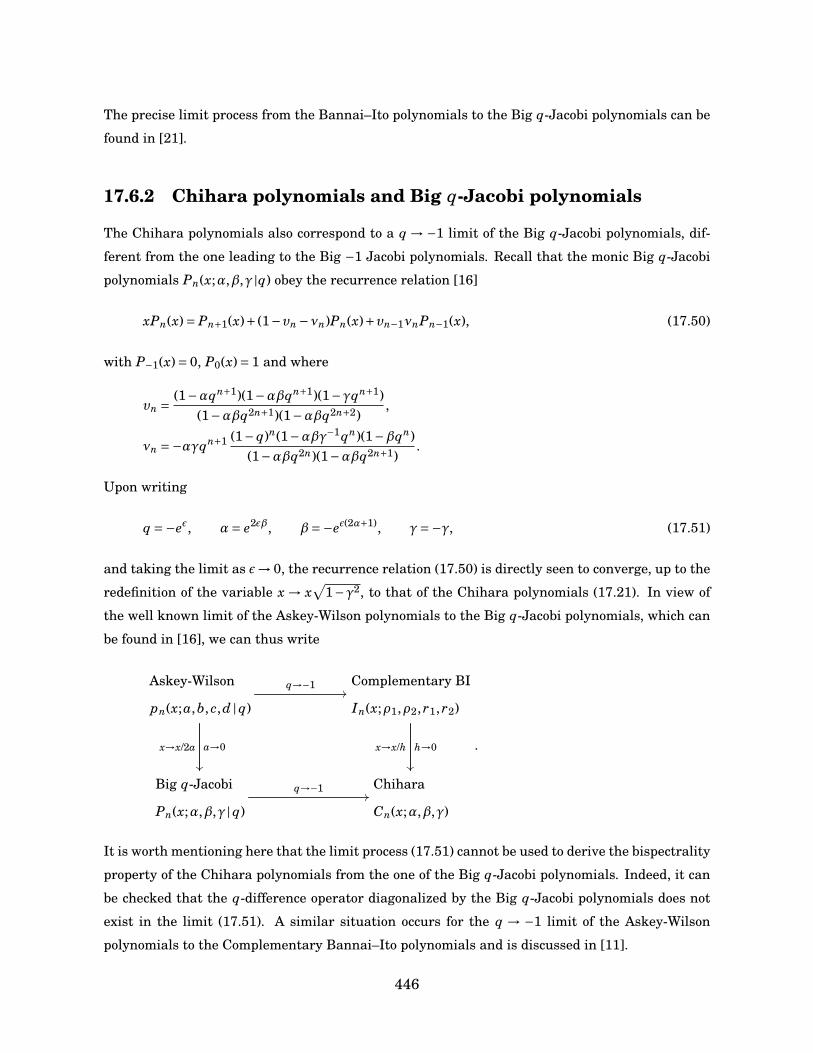
The precise limit process from the Bannai–Ito polynomials to the Big q-Jacobi polynomials can be
found in [21].
17.6.2 Chihara polynomials and Big q-Jacobi polynomials
The Chihara polynomials also correspond to a q →−1 limit of the Big q-Jacobi polynomials, dif-
ferent from the one leading to the Big −1 Jacobi polynomials. Recall that the monic Big q-Jacobi
polynomials Pn(x;α,β,γ |q) obey the recurrence relation [16]
xPn(x)= Pn+1(x)+ (1−υn −νn)Pn(x)+υn−1νnPn−1(x), (17.50)
with P−1(x)= 0, P0(x)= 1 and where
υn = (1−αqn+1)(1−αβqn+1)(1−γqn+1)(1−αβq2n+1)(1−αβq2n+2)
,
νn =−αγqn+1 (1− q)n(1−αβγ−1qn)(1−βqn)(1−αβq2n)(1−αβq2n+1)
.
Upon writing
q =−eε, α= e2εβ, β=−eε(2α+1), γ=−γ, (17.51)
and taking the limit as ε→ 0, the recurrence relation (17.50) is directly seen to converge, up to the
redefinition of the variable x → x√
1−γ2, to that of the Chihara polynomials (17.21). In view of
the well known limit of the Askey-Wilson polynomials to the Big q-Jacobi polynomials, which can
be found in [16], we can thus write
Askey-Wilson
pn(x;a,b, c,d |q)
q→−1//
a→0x→x/2a
Complementary BI
In(x;ρ1,ρ2, r1, r2)
h→0x→x/h
Big q-Jacobi
Pn(x;α,β,γ |q)
q→−1//Chihara
Cn(x;α,β,γ)
.
It is worth mentioning here that the limit process (17.51) cannot be used to derive the bispectrality
property of the Chihara polynomials from the one of the Big q-Jacobi polynomials. Indeed, it can
be checked that the q-difference operator diagonalized by the Big q-Jacobi polynomials does not
exist in the limit (17.51). A similar situation occurs for the q → −1 limit of the Askey-Wilson
polynomials to the Complementary Bannai–Ito polynomials and is discussed in [11].
446
17.7 Special cases and limits of Chihara polynomials
In this section, three special/limit cases of the Chihara polynomials Cn(x;α,β,γ) are considered.
One special case and one limit case correspond respectively to the generalized Gegenbauer and
generalized Hermite polynomials, which are well-known from the theory of symmetric orthogonal
polynomials [6]. The third limit case leads to a new bispectral family of −1 orthogonal polynomials
which depend on two parameters and which can be seen as a one-parameter extension of the
generalized Hermite polynomials.
17.7.1 Generalized Gegenbauer polynomials
It is easy to see from the explicit expression (17.20) that if one takes γ= 0, the Chihara polynomials
Cn(x;α,β,γ) become symmetric, i.e. Cn(−x) = (−1)nCn(x). Denoting by Gn(x;α,β) the polynomials
obtained by specializing the Chihara polynomials to γ= 0, one directly has
G2n(x)= (−1)n(α+1)n
(n+α+β+1)n2F1
[−n,n+α+β+1α+1
; x2],
G2n+1(x)= (−1)n(α+2)n
(n+α+β+2)nx 2F1
[−n,n+α+β+2α+2
; x2].
The polynomials Gn(x) are directly identified to the generalized Gegenbauer polynomials (see for
example [3, 7]). In view of proposition (4), the polynomials Gn(x) satisfy the recurrence relation
xGn(x)=Gn+1(x)+σn Gn−1(x),
with G−1(x)= 0, G0(x)= 1 and where σn is given by (17.22). It follows from proposition (5) that the
polynomials Gn(x) satisfy the family of eigenvalue equations
W (ε)Gn(x)=λ(ε)n Gn(x), (17.52)
where the eigenvalues are given by (17.24) and where the operator W (ε) has the expression
W (ε) = Sx ∂2x +Ux ∂x +Vx(I−R),
with the coefficients
Sx = x2 −14
, Ux = x2(α+β+3/2)−α−1/22x
, Vx = α+1/24x2 − α+β+3/2
4+ε/2.
Upon taking
ε→ (α+1)(µ+1/2), β→α, α→µ−1/2,
447
the eigenvalue equation (17.52) can be rewritten as
QGn(x)=ΥnGn(x), (17.53)
where
Q = (1− x2)[Dµx ]2 −2(α+1)xDµ
x , (17.54)
where Dµx stands for the Dunkl derivative operator
Dµx = ∂x + µ
x(I−R), (17.55)
and where the eigenvalues Υn are of the form
Υ2n =−2n(2n+2α+2µ+1), Υ2n+1 =−(2n+2µ+1)(2n+2α+2). (17.56)
The eigenvalue equation (17.53) with the operator (17.54) and eigenvalues (17.56) corresponds to
the one obtained by Ben Cheikh and Gaied in their characterization of Dunkl-classical symmetric
orthogonal polynomials [4]. The third proposition leads to the orthogonality relation∫ 1
−1Gn(x)Gm(x)ω(x) dx = knδnm,
where the normalization factor kn is given by (17.38) and where the weight function reads
ω(x)=|x|2α+1(1− x2)β.
We have thus established that the generalized Gegenbauer polynomials are −1 orthogonal poly-
nomials which are descendants of the Complementary Bannai–Ito polynomials.
17.7.2 A one-parameter extension
of the generalized Hermite polynomials
Another set of bispectral −1 orthogonal polynomials can be obtained upon letting
x →β−1/2x, α→µ−1/2, γ→β−1/2γ,
and taking the limit as β→∞. This limit is analogous to the one taking the Jacobi polynomials
into the Laguerre polynomials [16]. Let Yn(x;µ,γ) denote the monic polynomials obtained from the
Chihara polynomials in this limit. The following properties of these polynomials can be derived by
straightforward computations. The polynomials Yn(x;γ) have the hypergeometric expression
Y2n(x)= (−1)n(µ+1/2)n 1F1
[ −nµ+1/2
; x2 −γ2],
Y2n+1(x)= (−1)n(µ+3/2)n (x−γ) 1F1
[ −nµ+3/2
; x2 −γ2].
448

They satisfy the recurrence relation
xYn(x)=Yn+1(x)+ (−1)nγYn(x)+ϑn Yn−1(x),
with the coefficients
ϑ2n = n, ϑ2n+1 = n+µ+1/2.
The polynomials Yn(x;γ) obey the one-parameter family of eigenvalue equations
Z (ε)Yn(x)=λ(ε)n Yn(x),
where the spectrum has the form
λ(ε)2n = n, λ(ε)
2n+1 = n+ε.
The explicit expression for the second-order differential Dunkl operator Z (ε) is
Z (ε) = Sx ∂2x −Tx ∂xR+Ux ∂x +Vx(I−R),
with
Sx = γ2 − x2
4x2 , Tx = γ(x−γ)4x3 ,
Ux = x2+ γ
4x2 − γ2
2x3 − µ+γ2
2x, Vx = 3γ2
8x4 − γ
4x3 + µ+γ2
4x2 +ε x−γ2x
− 14
.
The algebra encoding this bispectrality of the polynomials Yn(x) is obtained by taking
K1 =Z (ε), K2 = x, P = R+ γ
x(I−R),
and defining K3 = [K1,K2]. One then has the commutation relations
[K1,P]= 0, K2,P= 2γ, K3,P= 0.
and
[K2,K3]= (2ε−1)K22P −2γK3P + (γ2 −2γε+µ)P +1/2,
[K3,K1]= (1−2ε)K3P +ε(ε−1)K2 +γε(ε−1)P.
The orthogonality relation reads∫S
Yn(x)Ym(x)w(x) dx = lnδnm
with S = (−∞,−|γ| ] ∪ [ |γ|,∞) and with the weight function
w(x)= θ(x)(x+γ) (x2 −γ2)µ−1/2 e−x2.
The normalization factors
l2n = n! e−γ2Γ(n+µ+1/2), l2n+1 = n! e−γ
2Γ(n+µ+3/2),
are obtained using the observation that the polynomials Yn(x;γ) can be expressed in terms of the
standard Laguerre polynomials [16].
449
17.7.3 Generalized Hermite polynomials
The polynomials Yn(x;µ,γ) can be can be considered as a one-parameter extension of the gener-
alized Hermite polynomials. Indeed, upon denoting by Hµn(x) the polynomials obtained by taking
γ= 0 in Yn(x;µ,γ), one finds that
Hµ
2n(x)= (−1)n(µ+1/2)n 1F1
[ −nµ+1/2
; x2],
Hµ
2n+1(x)= (−1)n(µ+3/2)n x 1F1
[ −nµ+3/2
; x2],
which corresponds to the generalized Hermite polynomials [6]. It is thus seen that the generalized
Hermite polynomials are also −1 orthogonal polynomials that can be obtained from the Comple-
mentary Bannai–Ito polynomials. For this special case, the eigenvalue equations can be written
(taking ε→ ε/2) as
Ω(ε)Hµn(x)=λ(ε)
n Hn(x),
with
λ(ε)2n = 2n, λ(ε)
2n+1 = 2n+ε.
and where the operator Ω(ε) reads
Ω(ε) =−12∂2
x +(x− µ
x
)∂x +
(µ
2x2 + ε−12
)(I−R).
The orthogonality relation then reduces to∫ ∞
−∞Hµ
n(x)Hµm(x) |x|µe−x2
dx = lnδnm.
Upon taking Ω(ε) = e−x2/2Ω(ε)ex2/2, the eigenvalue equations can be written as
Ω(ε)ψn(x)=λ(ε)n ψn(x),
with ψn = e−x2/2Hµn(x) and with the eigenvalues
λ(ε)2n = 2n+µ+1/2, λ(ε)
2n+1 = 2n+µ+3/2+ε.
The operator Ω(ε) can be cast in the form
Ω(ε) =−12
(Dµx )2 + 1
2x2 + ε
2(I−R),
where Dµx is the Dunkl derivative (17.55). The operator Ω(ε) corresponds to the Hamiltonian of the
one-dimensional Dunkl oscillator [20]. Two-dimensional versions of this oscillator models have
been considered recently [9, 10, 12].
450
17.8 Conclusion
In this paper, we have characterized a novel family of −1 orthogonal polynomials in a continuous
variable which are obtained from the Complementary Bannai–Ito polynomials by a limit process.
These polynomials have been called the Chihara polynomials and it was shown that they diag-
onalize a second-order differential Dunkl operator with a quadratic spectrum. The orthogonal-
ity weight, the recurrence relation and the explicit expression in terms of Gauss hypergeometric
function have also been obtained. Moreover, special cases and descendants of these Chihara poly-
nomials have been examined. From these considerations, it was observed that the well-known
generalized Gegenbauer/Hermite polynomials are in fact −1 polynomials. In addition, a new class
of bispectral −1 orthogonal polynomials which can be interpreted as a one-parameter extension of
the generalized Hermite polynomials has been defined.
With the results presented here, the polynomials in the higher portion of the emerging tableau
of −1 orthogonal polynomials are now identified and characterized. At the top level of the tableau
sit the Bannai–Ito polynomials and their kernel partners, the Complementary Bannai–Ito poly-
nomials. Both sets depend on four parameters. At the next level of this −1 tableau, with three
parameters, one has the Big −1 Jacobi polynomials, which are descendants of the BI polynomials,
as well as the dual −1 Hahn polynomials (see [22]) and the Chihara polynomials which are de-
scendants of the CBI polynomials. The complete tableau of −1 polynomials with arrows relating
them shall be presented in an upcoming review.
References
[1] R. Askey and J. Wilson. Some basic hypergeometric orthogonal polynomials that generalize
Jacobi polynomials. Mem. AMS, 54:1–55, 1985.
[2] E. Bannai and T. Ito. Algebraic Combinatorics I: Association Schemes. Benjamin/Cummings,
1984.
[3] S. Belmehdi. Generalized Gegenbauer orthogonal polynomials. J. Comp. Appl. Math.,
133:195–205, 2001.
[4] Y. Ben Cheikh and M. Gaied. Characterization of the Dunkl-classical symmetric orthogonal
polynomials. Appl. Math. Comp., 187:105–114, 2007.
[5] T. Chihara. On kernel polynomials and related systems. Boll. Un. Math. Ita., 19:451–459,
1964.
451
[6] T. Chihara. An Introduction to Orthogonal Polynomials. Dover Publications, 2011.
[7] C. F. Dunkl and Y. Xu. Orthogonal Polynomials of Several Variables. Cambridge University
Press, 2001.
[8] G. Gasper and M. Rahman. Basic Hypergeometric Series. Encyclopedia of Mathematics and
its Applications. Cambridge University Press, 2nd edition, 2004.
[9] V.X. Genest, M.E.H. Ismail, L. Vinet, and A. Zhedanov. The Dunkl oscillator in the plane:
I. Superintegrability, separated wavefunctions and overlap coefficients. J. Phys. A: Math.
Theor., 46:145201, 2013.
[10] V.X. Genest, M.E.H. Ismail, L. Vinet, and A. Zhedanov. The Dunkl oscillator in the plane: II.
Representations of the symmetry algebra. Comm. Math. Phys. (to appear), 2014.
[11] V.X. Genest, L. Vinet, and A. Zhedanov. Bispectrality of the Complementary Bannai–Ito
polynomials. SIGMA, 9:18–37, 2013.
[12] V.X. Genest, L. Vinet, and A. Zhedanov. The singular and 2:1 anisotropic Dunkl oscillators in
the plane. J. Phys. A: Math. Theor., 46:325201, 2013.
[13] V.X. Genest, L. Vinet, and A. Zhedanov. The Bannai-Ito polynomials as Racah coefficients of
the sl−1(2) algebra. Proc. Am. Soc., 142:1545–1560, 2014.
[14] J. Geronimus. The orthogonality of some systems of polynomials. Duke Math. J., 141:503–
510, 1947.
[15] Ya. A. Granovskii, I.M. Lutzenko, and A. Zhedanov. Mutual integrability, quadratic algebras,
and dynamical symmetry. Ann. Phys., 217:1–20, 1992.
[16] R. Koekoek, P.A. Lesky, and R.F. Swarttouw. Hypergeometric orthogonal polynomials and
their q-analogues. Springer, 1st edition, 2010.
[17] T. Koornwinder. On the Limit from q-Racah Polynomials to Big q-Jacobi Polynomials.
SIGMA, 7:40–47, 2011.
[18] D. Leonard. Orthogonal polynomials, duality and association schemes. SIAM J. Math. Anal.,
13, 1982.
[19] F. Marcellan and J. Petronilho. Eigenproblems for Tridiagonal 2-Toeplitz Matrices and
Quadratic Polynomial Mappings. Lin. Alg. Appl., 260:169–208, 1997.
452

[20] M. Rosenblum. Generalized Hermite polynomials and the Bose-like oscillator calculus. In
Nonselfadjoint Operators and Related Topics, Operator Theory: Advances and Applications.
Springer, 1994.
[21] S. Tsujimoto, L. Vinet, and A. Zhedanov. Dunkl shift operators and Bannai–Ito polynomials.
Adv. Math., 229:2123–2158, 2012.
[22] S. Tsujimoto, L. Vinet, and A. Zhedanov. Dual −1 Hahn polynomials: “Classical” polynomials
beyond the Leonard duality. Proc. Amer. Math. Soc., 141:959–970, 2013.
[23] L. Vinet and A. Zhedanov. A Bochner Theorem for Dunkl polynomials. SIGMA, 7:20–28,
2011.
[24] L. Vinet and A. Zhedanov. A ‘missing’ family of classical orthogonal polynomials. J. Phys. A:
Math. Theor., 44:085201, 2011.
[25] L. Vinet and A. Zhedanov. A limit q = −1 for the Big q-Jacobi polynomials. Trans. Amer.
Math. Soc., 364:5491–5507, 2012.
453

454
Chapitre 18
The Bannai–Ito polynomials as Racahcoefficients of the sl−1(2) algebra
V. X. Genest, L. Vinet et A. Zhedanov (2014). The Bannai–Ito polynomials as Racah coefficients of
the sl−1(2) algebra. Proceedings of the American Mathematical Society 142 1545-1560
Abstract. The Bannai-Ito polynomials are shown to arise as Racah coefficients for sl−1(2). This
Hopf algebra has four generators including an involution and is defined with both commutation
and anticommutation relations. It is also equivalent to the parabosonic oscillator algebra. The
coproduct is used to show that the Bannai-Ito algebra acts as the hidden symmetry algebra of the
Racah problem for sl−1(2). The Racah coefficients are recovered from a related Leonard pair.
Introduction
The sl−1(2) algebra was introduced recently in [20] as a deformation of the classical sl(2)
Lie algebra; it is defined in terms of four generators, including an involution, satisfying
both commutation and anticommutation relations. This algebra can also be obtained from
the quantum algebra slq(2) by taking the limit q →−1 and is furthermore the dynamical
algebra of a parabosonic oscillator [10, 13]. We here consider the Racah problem for this
algebra.
Recently, a series of orthogonal polynomials corresponding to limits q → −1 of q-
polynomials of the Askey scheme were discovered [19, 22, 25, 26]. These polynomials are
eigenfunctions of operators of Dunkl type, which involve the reflection operator [7, 24].
Interestingly, these polynomials have also been related to Jordan anticommutator alge-
bras [21]. In most references, so far, these q = −1 polynomials have been left buried in
the standard classifications. In view of their bispectrality and remarkable properties, a
−1 scheme would deserve to be highlighted.
At the top of the discrete variable branch of this q = −1 class of polynomials lie the
Bannai-Ito (BI) polynomials [2] and their kernel partners, the complementary Bannai-Ito
polynomials [22]. Both sets depend on four parameters and are expressible in terms of
Wilson polynomials [2, 12, 22]. The BI polynomials possess the Leonard duality property,
which in fact led to their initial discovery in [2]. In contradistinction, the complementary
BI polynomials and their descendants, the dual q = −1 Hahn polynomials [19], are also
bispectral but fall beyond the scope of the Leonard duality.
The Clebsch-Gordan problem for sl−1(2) was first solved in [20]; it was shown that
the coupling coefficients for two sl−1(2) algebras, also called Clebsch-Gordan or Wigner
coefficients, are proportional to the dual q = −1 Hahn polynomials [19]. In this paper,
we investigate the Racah problem for sl−1(2), which is tantamount to finding the cou-
pling coefficients for three parabosonic oscillators. It is shown that these coefficients are
also expressed in terms of q = −1 polynomials, in this case the Bannai-Ito polynomials.
Our approach consists in constructing the Jordan algebra of the intermediary Casimir
operators that appear in the coproduct [6] of three sl−1(2) algebras; this anticommutator
algebra coincides with the Bannai-Ito algebra [22], a special case of the Askey-Wilson al-
gebra introduced in [27]. The two Casimir operators are then shown to form a Leonard
pair [3, 5, 11, 16, 17, 18], an observation which allows to recover the recurrence relation
of the Bannai-Ito polynomials for the overlap (Racah) coefficients.
The outline of the paper is as follows. In section 1, we recall the definition of the sl−1(2)
algebra, its irreducible representations and its coproduct structure. We also provide a
review of the theory of the Bannai-Ito polynomials and go over the basics of Leonard
pairs and the corresponding Askey-Wilson relations [16, 23]. In section 2, we review
the Clebsch-Gordan problem for the parabosonic algebra sl−1(2). In section 3, we show
that the intermediary Casimir operators (K1,K2) of the sum of three sl−1(2) algebras
form the Bannai-Ito algebra. In section 4, the operators (K1,K2) are re-expressed as a
Leonard pair which is used to recover the recurrence relation satisfied by the overlap
coefficients (Racah) coefficients. The exact expression for the Racah coefficients is finally
obtained up to a phase factor using the orthogonality relation of the BI polynomials. In
section 5, we discuss the degenerate case of the Bannai-Ito algebra corresponding to the
anticommutator spin algebra [8, 14, 1, 3]. We conclude by explaining that the operators
K1 and K2, together with their anticommutator K3, form a Leonard triple. A different
456
Racah problem, which involves modifying the addition rule of sl−1(2), is considered to
that end.
18.1 The sl−1(2) algebra, Bannai-Ito polynomials and
Leonard pairs
18.1.1 sl−1(2) essentials
The Hopf algebra sl−1(2) [20] is generated by four operators J0, J+, J− and R satisfying
the relations
[J0, J±]=±J±, [J0,R]= 0, J+, J−= 2J0, J±,R= 0, (18.1)
where [x, y] = xy− yx and x, y = xy+ yx. The operator R is an involution, which means
that it satisfies the property
R2 = id, (18.2)
where id is the identity. The Casimir operator, which commutes with all sl−1(2) elements,
is given by
Q = J+J−R− J0R+R/2. (18.3)
Let ε=±1 and µ> 0 be two parameters; we denote by (ε,µ) the infinite-dimensional vector
space spanned by the basis | ε;µ;n ⟩, n ∈N, endowed with the actions
J0| ε;µ;n ⟩ = (n+µ+1/2)| ε;µ;n ⟩, R| ε;µ;n ⟩ = ε(−1)n| ε;µ;n ⟩,J+| ε;µ;n ⟩ =
√[n+1]µ| ε;µ;n+1 ⟩, J−| ε;µ;n ⟩ =
√[n]µ| ε;µ;n−1 ⟩,
(18.4)
where [n]µ denotes the µ-number
[n]µ = n+µ(1− (−1)n). (18.5)
With the actions (18.4), the vector space (ε,µ) forms an irreducible sl−1(2)-module. On
this module, the Casimir operator is a multiple of the identity
Q| ε;µ;n ⟩ =−εµ| ε;µ;n ⟩, (18.6)
457
as expected from Schur’s lemma. On the space (ε,µ), the algebra sl−1(2) is equivalent to
the parabosonic oscillator algebra. Indeed, one has
[J−, J+]= J−, J+−2J+J− = 2J0 −2J+J−. (18.7)
Using the expression (18.3) for the Casimir operator and its action on vectors of (ε,µ), we
find
[J−, J+]= 1+2εµR. (18.8)
The operators J± satisfying the commutation relation (18.8), together with the operator
R obeying the relations R2 = id and R, J± = 0, define the parabosonic oscillator algebra
[6, 13, 15].
The algebra sl−1(2) admits a non-trivial addition rule, or coproduct. Let (ε1,µ1) and
(ε2,µ2) be two sl−1(2)-modules. A third module can be obtained by taking tensor product
(ε1,µ1)⊗ (ε2,µ2) equipped with the transformations
J0(v⊗w)= (J0v)⊗w+v⊗ (J0w),
J±(v⊗w)= (J±v)⊗ (Rw)+v⊗ (J±w),
R(v⊗w)= (Rv)⊗ (Rw),
(18.9)
where v ∈ (ε1,µ1) and w ∈ (ε2,µ2). The addition rule for sl−1(2) can also be presented
without referring to any representation. Let J(i)0 , J(i)
± and R(i) be two mutually commuting
sets of sl−1(2) generators. A third algebra, denoted symbolically 3 = 1⊕2, is obtained by
defining
J(3)0 = J(1)
0 + J(2)0 , J(3)
± = J(1)± R(2) + J(2)
± , R(3) = R(1)R(2). (18.10)
It is easily verified that the generators J(3)0 , J(3)
± and R(3) satisfy the defining relations of
sl−1(2) given in (18.1). The Casimir operator for the third algebra, denoted by Q12, is
Q12 = J(3)+ J(3)
− R(3) − J(3)0 R(3) + (1/2)R(3) (18.11)
18.1.2 Bannai-Ito polynomials
Bannai and Ito discovered their polynomials in 1984 in their complete classification of
orthogonal polynomials satisfying the Leonard duality property [2]. These polynomials
were shown to be q =−1 limits of the q-Racah polynomials and many of their properties
458
(e.g. recurrence relation, weight function, hypergeometric representation) were given in
their book [2]. Recently, it was shown in [22] that the Bannai-Ito polynomials also occur
naturally as eigensolutions of Dunkl shift operators.In the following, we review some of
the properties of the BI polynomials.
The monic BI polynomials satisfy the recurrence relation
Pn+1(x)+ (ρ1 − An −Cn)Pn(x)+ An−1CnPn−1(x)= xPn(x), (18.12)
where
An =
(n+1+2ρ1−2r1)(n+1+2ρ1−2r2)
4(n+1−r1−r2+ρ1+ρ2) , n even,(n+1−2r1−2r2+2ρ1+2ρ2)(n+1+2ρ1+2ρ2)
4(n+1−r1−r2+ρ1+ρ2) , n odd,(18.13)
Cn =
− n(n−2r1−2r2)4(n−r1−r2+ρ1+ρ2) , n even,
− (n−2r2+2ρ2)(n−2r1+2ρ2)4(n−r1−r2+ρ1+ρ2) , n odd.
(18.14)
The polynomials satisfying (18.12) are called positive definite if Un = An−1Cn > 0 for all
n > 1. This condition is also equivalent to the existence of a positive orthogonality mea-
sure for the polynomials Pn(x). In the case of the BI polynomials, it is seen that this condi-
tion cannot be fulfilled for all values of n. However, if Ui > 0 for i = 1, . . . , N and UN+1 = 0,
it is known that one has a finite system of orthogonal polynomials P0(x), P1(x), . . . , PN(x)
satisfying the discrete orthogonality relation
N∑s=0
ωs(xs)Pn(xs)Pm(xs)= hnδnm, hn = u1, . . . ,un, (18.15)
on the lattice xs, where s = 0,1, . . . , N. The discrete points xs are the simple roots of the
polynomial PN+1(x) [4].
When N is an even integer, the truncation condition UN+1 = 0 is equivalent to one of
the four possible conditions
2(r i −ρk)= N +1, i,k = 1,2. (18.16)
The case of relevance here is
2(r2 −ρ1)= N +1. (18.17)
We introduce the following parametrization:
2ρ1 = (b+ c), 2ρ2 = (2a+b+ c+N +1),
2r1 = (c−b), 2r2 = (b+ c+N +1),(18.18)
459
where a, b and c are arbitrary positive parameters. Assuming (18.18), the coefficient Un
takes the form:
Un =
n(N+2c+1−n)(n+2a+2b)(n+2a+2b+2c+N+1)
16(a+b+n)2 , n even,(N+1−n)(2a+n)(2b+n)(n+2a+2b+N+1)
16(a+b+n)2 , n odd.(18.19)
From this expression, it is obvious that UN+1 = 0 and that the positivity condition Un > 0
is satisfied for n = 0, . . . , N. With this parametrization, the Bannai-Ito polynomials obey
the orthogonality relation
∑N`=0Ω`Pn(x`)Pm(x`)=ΦN,nδnm. (18.20)
The orthogonality grid is given by
x` = 12
[(−1)`(`+b+ c+1/2)−1/2
]. (18.21)
The weight function Ω` takes the form
Ω` = (−1)q (−N/2)k+q(1/2+b)k+q(1+b+ c)k(3/2+a+b+ c+N/2)k
(1/2+ c)k+q(1+b+ c+N/2)k+q(1/2−a−N/2)kk!, (18.22)
where `= 2k+q with q = 0,1 and where (x)n = (x)(x+1) · · · (x+n−1) stands for the Pochham-
mer symbol. Furthermore, the normalization factor ΦN,n is found to be
ΦN,n = m!k!(m−k− q)!
[(1+a+b+k)m−k(1+b+ c)m
(1/2+a+k+ q)m−k−q(1/2+ c)m−k
]×
[(1/2+b)k+q(m+1+a+b)k+q(m+3/2+a+b+ c)k
(k+1+a+b)2k+q
], (18.23)
where m = N/2 and n = 2k+q with q = 0,1. The other truncation conditions in (18.16) can
be treated similarly.
When N is an odd integer, the truncation condition UN+1 = 0 is equivalent to one of
the three conditions
i) ρ1 +ρ2 =−N +12
, ii) r1 + r2 = N +12
,
iii) ρ1 +ρ2 − r1 − r2 =−N +12
.(18.24)
The condition iii) leads to a singular Un for n = (N +1)/2. Consequently, only the condi-
tions i) and ii) are admissible. The case of relevance here is
2(ρ1 +ρ2)=−(N +1). (18.25)
460
We introduce the following parametrization:
2ρ1 = (β+γ), 2ρ2 =−(β+γ+N +1),
2r1 = (γ−β), 2r2 =−(2α+β+γ+N +1),(18.26)
where α, β and γ are arbitrary positive parameters. Assuming (18.26), the coefficient Un
becomes
Un =
n(N+1−n)(n+2α+2β)(n+2α+2β+N+1)
16(α+β+n)2 , n even,(N+2γ+1−n)(2α+n)(2β+n)(n+2α+2β+2γ+N+1)
16(α+β+n)2 , n odd.(18.27)
In this form, the truncation and positivity conditions are manifestly satisfied. With these
parameters, the Bannai-Ito polynomials obey the orthogonality relation
N∑`=0
Ω`Pn(x`)Pm(x`)=ΦN,nδnm. (18.28)
The grid is given by
x` = 12
[(−1)`(`+β+γ+1/2)−1/2
]. (18.29)
The weight function takes the form
Ω` = (−1)q (1−N2 )k(1
2 +β)k+q(1+β+γ)k(1+α+β+γ+ N2 )k+q
(12 +γ)k+q(−α− N
2 )k+q(32 +β+γ+ N
2 )kk!, (18.30)
where `= 2k+ q with q = 0,1 and the normalization factor can be evaluated to
ΦN,n = (m−1)!k!(m−k−1)!
[(1+α+β+k)m−k(1+β+γ)m
(1/2+k+ q+α)m−k−q(1/2+γ)m−k−q
]×
[(1/2+β)k+q(m+1+α+β)k(m+1/2+α+β+γ)k+q
(k+1+α+β)2k+q
], (18.31)
where m = (N +1)/2 and n = 2k+ q with q = 0,1.
The Bannai-Ito polynomials correspond to the limit q → −1 of the classical Wilson
polynomials and admit a hypergeometric representation. The truncated generalized hy-
pergeometric series is defined by
p+1Fq
(−n, a1, . . . ,ap
b1, b2, . . . ,bq; x
)=
n∑j=0
(−n) j(a1) j · · · (ap) j
(b1) j(b2) j · · · (bq) j
x j
j!. (18.32)
461
We define
W2n(x)= κ(1)n 4F3
(−n, n+ g+1, ρ2 + x, ρ2 − x
ρ1 +ρ2 +1, ρ2 − r1 + 12 , ρ2 − r2 + 1
2
;1
), (18.33)
W2n+1(x)= κ(2)n (x−ρ2)4F3
(−n, n+ g+2, ρ2 +1+ x, ρ2 +1− x
ρ1 +ρ2 +2, ρ2 − r1 + 32 , ρ2 − r2 + 3
2
;1
), (18.34)
with g = ρ1 +ρ2 − r1 − r2 and where the factors which ensure that the polynomials are
monic are given by
κ(1)n = (1+ρ1 +ρ2)n(ρ2 − r1 +1/2)n(ρ2 − r2 +1/2)n
(n+ g+1)n, (18.35)
κ(2)n = (2+ρ1 +ρ2)n(ρ2 − r1 +3/2)n(ρ2 − r2 +3/2)n
(n+ g+2)n. (18.36)
The monic BI polynomials have the following expression:
Pn(x)=Wn(x)−CnWn−1(x), (18.37)
where Cn is given by (18.13).
18.1.3 Leonard pairs and Askey-Wilson relations
Let V be a C-vector space of dimension N + 1. A square matrix X is said irreducible
tridiagonal if each of its non-zero entry lies on either the diagonal, sub-diagonal or super-
diagonal and if each entry on the super-diagonal and sub-diagonal are non-zero. A Leo-
nard pair on V is an ordered pair of linear transformations (K1,K2) ∈EndV satisfying the
following conditions [16]:
• There exists a basis for V with respect to which the matrix representing K1 is diag-
onal and the matrix representing K2 is irreducible tridiagonal.
• There exists a basis for V with respect to which the matrix representing K2 is diag-
onal and the matrix representing K1 is irreducible tridiagonal.
Leonard pairs have deep connections with orthogonal polynomials on finite grids and
have also appeared in combinatorics [2, 16]. Given a Leonard pair (K1,K2), it is known
[18, 23, 27] that K1, K2 obey the so-called Askey-Wilson relations
K21K2 −βK1K2K1 +K2K2
1 −γ1K1,K2−ρ1K2 = γ2K21 +ωK1 +η1id,
K22K1 −βK2K1K2 +K1K2
2 −γ2K1K2−ρ2K2 = γ1K21 +ωK1 +η2id,
(18.38)
462

with scalars β,γi,ηi,ρ i ∈C. These scalars are uniquely defined provided that the dimen-
sion of the vector space is at least 4. The converse is not always true. Indeed, if one sets
β= q+ q−1 and q a root of unity, two linear transformations obeying relations (18.38) do
not necessarily form a Leonard pair [17]. In the present work we will nonetheless obtain
a Leonard pair satisfying the relations (18.38) with q =−1.
We briefly recall how orthogonal polynomials occur in this context. Consider a Leonard
pair (K1,K2) on a vector space V of dimension N +1. By definition, the eigenvalues of K1
and K2 are mutually distinct. Denoting the eigenvalues of K1 by λ(1)i for i = 0,1, . . . , N,
there exists a basis of V in which the matrices representing K1 and K2 are of the form
K1 =
λ(1)
0 0λ(1)
1. . .
0 λ(1)N
, K2 =
a0 c1 0x0 a1 c2
x1 a2. . .
. . . . . . cN
0 xN−1 aN
. (18.39)
One can define the sequence of polynomials pi with i = 0, . . . , N and initial condition p−1 =0 satisfying the recurrence relation
y pi(y)= ci+1 pi+1(y)+ai pi(y)+ xi−1 pi−1(y). (18.40)
The matrix Pi j = pi(λ(2)j ), where λ(2)
j , j ∈ 0,1, . . . , N, denotes the eigenvalues of K2, de-
fines the similarity transformation which brings the matrix K2 to its diagonal form. In
physical terms, given a pair (K1,K2) of operators expressed in the form (18.39) acting on
a state space, the polynomials defined by the recurrence relation (18.40) are the overlap
coefficients between the bases in which either K1 or K2 is diagonal. For more details, see
[16].
18.2 The Clebsch-Gordan problem
The Clebsch-Gordan (CG) problem of sl−1(2) has been solved in [20]. We recall here some
of the results concerning this problem which shall prove useful.
The CG problem can be posited in the following way. We consider the sl−1(2)-module
(ε1,µ1)⊗ (ε2,µ2) or equivalently the addition of two sl−1(2) algebras. It is seen that the
operator J(3)0 = J(1)
0 + J(2)0 has eigenvalues of the form µ1 +µ2 + N +1, N ∈ N. We denote
463

by | q12, N ⟩ the state with eigenvalue q12 of the Casimir operator Q12 and with a given
value N of the total projection. We have
Q12| q12, N ⟩ = q12| q12, N ⟩, J(3)0 | q12, N ⟩ = (µ1 +µ2 +1+N)| q12, N ⟩. (18.41)
In view of the formula (18.6), the eigenvalues q12 of the Casimir operator Q12 can be
decomposed as the product
q12 =−ε12µ12, ε12 =±1, µ12 > 0, (18.42)
whence we have |q12| = µ12. The Casimir operator (18.11) of the added algebras can be
re-expressed in terms of the local Casimir operators Q1 and Q2 in the following way:
Q12 =(J(1)− J(2)
+ − J(1)+ J(2)
−)R(1) − (1/2)R(1)R(2) +Q1R(2) +Q2R(1). (18.43)
The state | q12, N ⟩ can be decomposed as a linear combination of the tensor product states
| q12, N ⟩ = ∑n1+n2=N
Cµ1µ2q12n1n2N | ε1,µ1,n1 ⟩⊗| ε2,µ2,n2 ⟩. (18.44)
The coefficients Cµ1µ2q12n1n2N are the Clebsch-Gordan coefficients of the sl−1(2) algebra. We
note that these coefficients vanish unless n1+n2 = N and that their dependence on ε1 and
ε2 is implicit.
The possible values of the eigenvalues q12 of the Casimir operator Q12 are given by
q12 = (−1)s+1ε1ε2(µ1 +µ2 +1/2+ s), s = 0,1, . . . , N. (18.45)
This result can be derived in the following way. In a given module (ε,µ), the eigenvalues
λJ0 of J0 are
λJ0 = n−εQ+1/2, n ∈N. (18.46)
Hence, for a given eigenvalue λJ0 > 0 of J0, the eigenvalues q of the Casimir operator Q
which are compatible with λJ0 are, in absolute value,
|q| = |λ−1/2|, |λ−3/2|, . . . (18.47)
When considering the coproduct of two sl−1(2) algebras, the eigenvalues of J(3)0 are λ(3) =
µ1 +µ2 + N +1. Consequently, for a given value of N, the set of allowed values for the
eigenvalues q12 of the Casimir Q12, which should be of cardinality N +1, is
|q12| =µ1 +µ2 +N +1/2, µ1 +µ2 +N −1/2, . . . ,µ1 +µ2 +1/2. (18.48)
464
Thus the admissible values of µ12 = |q12| are given by the above set (18.48).
There remains to evaluate the corresponding values of ε12. To that end, we consider
the eigenstate | x ⟩ of Q12 corresponding to the maximal value µ12)max = µ1 +µ2 +N +1/2.
It is seen that this state satisfies the properties
J(3)0 | x ⟩ = (µ1 +µ2 +N +1)| x ⟩, J(3)
− | x ⟩ = 0. (18.49)
On the one hand, it then follows from (18.49) and (18.4) that
R(3)| x ⟩ = ε12)max| x ⟩, (18.50)
where ε12)max is the value of ε12 corresponding to the maximal value of µ12. On the other
hand, it stems from (18.41) and (18.4) that
R(3)| q12, N ⟩ = (−1)Nε1ε2| q12, N ⟩. (18.51)
We thus have ε12)max = (−1)Nε1ε2. It follows that the eigenvalue q12 of the Casimir oper-
ator Q12 corresponding to the maximal value of |q12| is given by
q12 = (−1)N+1ε1ε2(µ1 +µ2 +1/2+N). (18.52)
By induction on N, one is led to the announced form of the eigenvalues (18.45). The
Casimir operator Q12 is tridiagonal in the tensor product basis. This allows to obtain a
recurrence relation for the Clebsch-Gordan coefficients which, given the spectrum (18.45),
is seen to coincide with that of the dual −1 Hahn polynomials [19, 20].
18.3 The Racah problem and Bannai-Ito algebra
The addition rule (18.10) possess an associativity property when three sl−1(2) algebras
are added. We consider three mutually commuting sets of sl−1(2) generators J( j)0 , J( j)
± and
R( j) for j = 1,2,3. The resulting fourth algebra can be obtained by two different addition
sequences. Indeed, one has the two equivalent schemes: 4 = (1⊕2)⊕3 and 4 = 1⊕ (2⊕3).
The Racah problem consists in finding the overlap between the respective eigenstates of
the intermediary Casimir operators Q12 and Q23 with a fixed eigenvalue q4 of the total
Casimir operator Q4. Denoting such eigenstates by | q12; q4,m ⟩ and | q23; q4,m ⟩, the
Racah coefficients are defined as
| q12; q4,m ⟩ = ∑q23
Rµ1µ2µ3q12q23µ4 | q23; q4,m ⟩, (18.53)
465
where we have by definition
Q12| q12, q4,m ⟩ = q12| q12, q4,m ⟩, Q23| q23, q4,m ⟩ = q23| q23, q4,m ⟩. (18.54)
We note that the Racah coefficients Rµ1µ2µ3q12q23µ4 do not depend on the total projection num-
ber m and that their dependence on εi, i ∈ 1, . . . ,4, is implicit. The problem of finding
the overlap coefficients is non-trivial because the operators Q12 and Q23 do not commute,
hence they cannot be simultaneously diagonalized. The two intermediary Casimir opera-
tors have the following expressions:
K1 =Q12 =(J(1)− J(2)
+ − J(1)+ J(2)
−)R(1) −R(1)R(2)/2+Q1R(2) +Q2R(1), (18.55)
K2 =Q23 =(J(2)− J(3)
+ − J(2)+ J(3)
−)R(2) −R(2)R(3)/2+Q2R(3) +Q3R(2). (18.56)
The full Casimir operator of the fourth algebra Q4 can also be obtained in a straightfor-
ward manner; one finds
Q4 =(J(1)− J(3)
+ − J(1)+ J(3)
−)R(1) −Q2R(1)R(3) +Q12R(3) +Q23R(1). (18.57)
The paramount observation is that the operators K1, K2 are closed in frames of a simple
algebra with three generators. To see this, one first defines
K3 = (J(1)+ J(3)
− − J(1)− J(3)
+ )R(1)R(2) +R(1)R(3)/2−Q1R(3) −Q3R(1). (18.58)
Since the operators Qi for i = 1, . . . ,4 commute with K1, K2, K3 and among themselves,
we shall replace them by their corresponding eigenvalues −λ j where λ j = ε jµ j. A direct
computation shows that the following relations hold:
K1,K2= K3 +α3, K2,K3= K1 +α1, K1,K3= K2 +α2, (18.59)
where the structure constants are given by
α1 =−2(λ1λ2 +λ3λ4), α2 =−2(λ1λ4 +λ2λ3), α3 = 2(λ1λ3 +λ2λ4). (18.60)
Note that the first relation of (18.59) can be considered as a definition of K3. The algebra
(18.59) is known as the Bannai-Ito algebra [22], which is, as will be seen below, a special
case of the Askey-Wilson algebra (18.38). It admits the Casimir operator
QBI = K21 +K2
2 +K23 , (18.61)
466
which commutes with all generators. Given the realization (18.60) of this algebra, the
Casimir operator takes the value
QBI =λ21 +λ2
2 +λ23 +λ2
4 −1/4. (18.62)
We now look to construct irreducible BI-modules; the degree of these representations
is prescribed by the range of possible eigenvalues of the operators Q12 and Q23. For
simplicity, we restrict ourselves to the case where ε1, ε2 and ε3 are all equal to 1. The
other cases can be treated in similar fashion. It is worth mentioning that ε4 cannot be
fixed a priori and will in fact depend on the degree of the given module.
In the CG problem, the possible eigenvalues of q12 were determined by the value of the
total projection operator. For the Racah problem, the overlap coefficients are independent
of the total projection and the spectrum of Q12 is restricted only by the value of the total
Casimir operator Q4. From (18.48), one finds that the minimal value of the absolute value
of q12 is given by
|q12|min =µ1 +µ2 +1/2. (18.63)
In addition, in view of the addition scheme 4= (1⊕2)⊕3, we have that the absolute value
of the eigenvalues q4 of the total Casimir operator Q4 are of the form
|q4| = |q12|+µ3 +1/2+ s12,3, s12,3 = 0,1, . . . ,m (18.64)
where m is the total projection of the state | q12; q4,m ⟩. It is clear that for a given absolute
value of |q4| = µ4, the maximal value of |q12| corresponds to setting s12,3 = 0. It then
follows that
|q12|max =µ4 −µ3 −1/2. (18.65)
Considering finite-dimensional representations of degree N +1, we find from (18.63) that
the eigenvalues q12 of the Casimir Q12 are of the form
|q12| =µ1 +µ2 +1/2,µ1 +µ2 +3/2, . . . ,µ1 +µ2 +1/2+N. (18.66)
Using (18.65) and (18.66), we obtain
N +1=µ4 −µ1 −µ2 −µ3. (18.67)
467

The spectra of the intermediary Casimir operators Q12 and Q23 are thus given by
q12 = (−1)s12+1(µ1 +µ2 +1/2+ s12), s12 = 0, . . . , N, (18.68)
q23 = (−1)s23+1(µ2 +µ3 +1/2+ s23), s23 = 0, . . . , N. (18.69)
The parameter ε4 is prescribed by the value of N. Indeed, from the CG problem it is
known that the allowed eigenvalues q4 of the Casimir operator Q4 are of the form
q4 = (−1)k+1(µ12 +µ3 +1/2+k), k = 0, . . . ,m (18.70)
where m is the total projection. Taking into account the condition (18.67), one finds
ε4 = (−1)N . (18.71)
Having found the explicit expressions for the spectra and dimension in terms of the rep-
resentation parameters, the matrix representation of the BI algebra can be made explicit.
18.4 Leonard pair and Racah coefficients
Let µ1, µ2, µ3 be fixed (positive) representation parameters and N a positive integer as
in (18.67). The operators K1, K2 are square matrices of dimension N +1 which are easily
seen to satisfy the following Askey-Wilson relations:
K21K2 +2K1K2K1 +K2K2
1 −K2 = κ3K1 +κ2, (18.72)
K22K1 +2K2K1K2 +K1K2
2 −K1 = κ3K2 +κ1, (18.73)
where the constants κi, i = 1,2,3, are given by
κ1 =−2(µ1µ2 +ε4µ3µ4),
κ2 =−2(µ2µ3 +ε4µ1µ4),
κ3 = 4(µ1µ3 +ε4µ2µ4),
(18.74)
with ε4 = (−1)N . The matrix representing K1 can be made diagonal with eigenvalues
prescribed by (18.68) and (18.54). In this basis, it is easily seen that the relations (18.72)
and (18.73) imply that K2 must be irreducible tridiagonal. The pair (K1,K2) thus forms a
Leonard pair. Consequently, there exists a basis in which the matrices K1 and K2 can be
468
expressed as
K1 = diag(θ0,θ1, · · · ,θN), K2 =
b0 1 0u1 b1 1
u2 b2 1. . . . . . . . .
bN−1 1
0 uN bN
, (18.75)
where θi = (−1)i+1(µ1+µ2+1/2+ i) for i = 0, . . . , N and un, bn are indeterminate. Imposing
the relations (18.72) and (18.73) on the two operators and solving for bn and un, one finds
−bn =
(µ2 +µ3 +1/2)+ 12
n(n+µ1+µ2−µ3−ε4µ4)(n+µ1+µ2)
−12
(n+1+2µ2)(n+1+µ1+µ2+µ3−ε4µ4)(n+1+µ1+µ2) , for n even,
(µ2 +µ3 +1/2)+ 12
(n+2µ1)(n+µ1+µ2−µ3+ε4µ4)(n+µ1+µ2)
−12
(n+1+2µ1+2µ2)(n+1+µ1+µ2+µ3+ε4µ4)(n+1+µ1+µ2) , for n odd,
(18.76)
un =
−14
n(n+2µ1+2µ2)(n+µ1+µ2+µ3+ε4µ4)(n+µ1+µ2−µ3−ε4µ4)(n+µ1+µ2)2 , for n even,
−14
(n+2µ2)(n+2µ1)(n+µ1+µ2+µ3−ε4µ4)(n+µ1+µ2−µ3+ε4µ4)(n+µ1+µ2)2 , for n odd.
(18.77)
The overlap coefficients of the bases in which either Q12 or Q23 is diagonal will thus be
proportional to the monic polynomials Pn(θ∗i ) with θ∗i = (−1)i+1(µ2+µ3+1/2+ i) which obey
the recurrence relation
Pn+1(x)+bnPn(x)+unPn−1(x)= xPn(x). (18.78)
Defining Pn(x) = (−2)−nPn(x), we recover the recurrence relation of the monic Bannai-Ito
polynomials
Pn+1(xs)+ (ρ1 − An −Cn)Pn(xs)+ An−1CnPn(xs)= xsPn(xs), (18.79)
with xs =−θ∗s /2−1/4 and where the identification with the Bannai-Ito parameters is
ρ1 = 12
(µ2 +µ3), ρ2 = 12
(µ1 +ε4µ4),
r1 = 12
(µ3 −µ2), r2 = 12
(ε4µ4 −µ1).(18.80)
469
The coefficients An and Cn are as defined in (18.13). The truncation conditions are the
following. On the one hand, if N is even, we have
2(r2 −ρ1)= N +1, (18.81)
as well as the identification a = µ1, b = µ2 and c = µ3. On the other hand, if N is odd, we
have
2(ρ1 +ρ2)=−(N +1), (18.82)
and the identification α=µ1, β=µ2 and γ=µ3. Is is seen that the Bannai-Ito grids (18.21)
and (18.29) coincide, as expected, with the predicted spectrum of the Casimir operator
Q23. To determine the normalization constant, we use the unitarity of the transformation
which imposes the following orthogonality relation for Racah coefficients:∑q23
Rµ1µ2µ3qq23µ4 Rµ1µ2µ3
q′q23µ4= δqq′ . (18.83)
Using the relations (18.20), (18.28) and (18.83), we obtain
Rµ1µ2µ3q12q23µ4 =
√Ω`(x`)ΦN,n
Pn(ρ1,ρ2, r1, r2; x`), (18.84)
where Pn(ρ1,ρ2, r1, r2; x`) is the monic Bannai-Ito polynomial. In addition, we have
x` =−12
(θ∗` +1/2
), `= |q23|−µ2 −µ3 −1/2, n = |q12|−µ1 −µ2 −1/2, (18.85)
along with the identifications (18.67), (18.80), (18.81) and (18.82). The Racah coeffi-
cients (18.84) are thus determined up to a phase factor. Returning the Bannai-Ito al-
gebra (18.59), it is seen that the realization (18.60) is invariant under the permuta-
tions π1 = (12)(34), π2 = (13)(24) and π3 = (14)(23) of the representation parameters λi,
i = 1, . . .4. These transformations generate the Klein four-group. In addition, the opera-
tion λi →−λi also leaves (18.59) and (18.60) invariant.
18.5 The Racah problem for the addition of ordinary
oscillators
When µ = 0, the sl−1(2) algebra reduces to the Heisenberg oscillator algebra endowed
however with a non-trivial coproduct. Therefore, the algebra obtained from the Hopf
470
addition rule (18.10) of two sl−1(2) algebras with µi = 0 is not as a result a pure oscilla-
tor algebra, but a parabosonic algebra. The same assertion holds for the addition of three
sl−1(2) algebras with Casimir parameters µ1, µ2 and µ3 all equal to zero. This corresponds
to adding three pure oscillator algebras with the addition rule (18.10). Due to the impor-
tance of the oscillator algebra, it is worth recording this reduction in some detail. Most
algebraic results connected to this skewed addition of three quantum harmonic oscillators
have interestingly been obtained previously in [8, 14, 1, 3]. In the case µ1 = µ2 = µ3 = 0,
the Bannai-Ito (18.59) algebra becomes
K1,K2= K3, K2,K3= K1, K1,K3= K2. (18.86)
This algebra can be seen as an anti-commutator version of the classical su(2) Lie algebra.
The Askey-Wilson relations simplify to
K21K2 +2K1K2K1 +K2K2
1 −K2 = 0, (18.87)
K22K1 +2K2K1K2 +K1K2
2 −K1 = 0. (18.88)
The spectra of the operators K1 and K2 are then given by the formula
θi = (−1)i+1(i+1/2). (18.89)
Moreover, the degree of the module is N+1=µ4 with ε4 = (−1)N . With these observations,
the pair (K1,K2) again forms a Leonard pair. The matrices K1 and K2 can thus be put in
the form
K1 = diag(θ0,θ1, · · · ,θN), K2 =
b0 1 0u1 b1 1
u2 b2 1. . . . . . . . .
bN−1 1
0 uN bN
. (18.90)
In this case, solving for the coefficients bn and un yields on the one hand
b0 =−(N +1)/2, and bi = 0 for i 6= 0, (18.91)
and on the other hand
un = (n+N +1)(N +1−n)4
. (18.92)
471
The positivity and truncation conditions un > 0 and uN+1 are manifestly satisfied here.
As expected, the obtained sequences bn, un correspond to the specializations µ1 =µ2 =µ3 = 0 of the formulas (18.76) and (18.77). Similarly to the Bannai-Ito case, the similarity
transformation bringing K2 into its diagonal form can be constructed with the Bannai-
Ito polynomials reduced with the parametrizations a = 0, b = 0 and c = 0 in the N even
case and α= 0, β= 0 and γ= 0 in the N odd case. The explicit hypergeometric represen-
tation (18.37) of the corresponding polynomials, the weight functions (18.22), (18.30) as
well as the normalization constants can be imported directly without need of a limiting
procedure.
Conclusion: the Leonard triple
We considered the Racah problem for the algebra sl−1(2) which acts as the dynamical alge-
bra for a parabosonic oscillator and showed that the algebra of the intermediary Casimir
operators coincide with the Bannai-Ito algebra. From the knowledge of the Clebsch-
Gordan problem, the spectra of the Casimir operators were determined and this allowed
to build the relevant finite-dimensional modules for the BI algebra. It was then recog-
nized that the operators Q12 = K1 and Q23 = K2 form a Leonard pair and this observation
was used to see that the overlap (Racah) coefficients are given in terms of the Bannai-Ito
polynomials.
As is manifest from (18.59), the Bannai-Ito algebra has a Z3 symmetry with respect
to a relabeling of the operators K i with i = 1,2,3. However, the Racah problem considered
here provides a specific realization of the BI algebra in terms of the distinct operators
Q12, Q23 and K3, for which this symmetry is not present. In this regard, it is natural
to ask whether there exists a situation for which it is the pair (K2,K3) or (K1,K3) that is
realized by intermediate Casimir operators. This question can answered by considering
the Racah problem for the addition of three sl−1(2) algebras with different addition rules
that lead to a fourth algebra that has nevertheless the same total Casimir Q4. The first
intermediate algebra (31)= 3⊕ 1 is obtained by defining
J(31)0 = J(1)
0 + J(3)0 , J(31)
± = J(1)± R(3) + J(3)
± R(2), R(31) = R(1)R(3), (18.93)
which differs from the original coproduct by the presence of R(2). Note that (18.93) im-
plicitly uses (ε2,µ2) as an auxiliary space. The intermediate Casimir operator Q13 is then
472
found to coincide with the negative of K3 as defined in (18.58):
Q31 =−K3. (18.94)
A second intermediate Casimir operator is obtained by using the standard coproduct
(18.10) in two ways: one forms the algebra (12), for which Q12 = K1, or one forms the
algebra (23) for which Q23 = K2. To ensure consistency, as mentioned before, the full
Casimir operator of the fourth algebra (4)= (31)⊕ (2) should coincide with (18.57). This is
done by defining
J(4)0 = J(31)
0 + J(2)0 , J(4)
± = J(31)± R(2) + J(2)
± R(3), R(4) = R(31)R(2), (18.95)
It is readily seen that the generators defined in (18.93) and (18.95) satisfy the defining re-
lations (18.1) of sl−1(2). This fourth algebra is easily seen to admit the same full Casimir
operator (18.57). Defining K3 = −Q31, K1 = K1 and K2 = K2, the algebra (18.59) is re-
covered with the pair (K1, K3) or (K2, K3) playing the role of the intermediate Casimir
operators. The steps of Sections 3, 4 can then be reproduced and this leads one to con-
clude that K3 also has a Bannai-Ito type spectrum λ(3)i = (−1)i(µ1+µ3+1/2+ i), i = 0, . . . , N
and that (K2,K3) and (K1,K3) form Leonard pairs. In addition, it follows from this obser-
vation that in the realization (18.60) of the Bannai-Ito algebra (18.59) obtained from the
operators (18.55), (18.56) and (18.58), the set (K1,K2,K3) constitutes a Leonard Triple,
which have studied intensively for the q-Racah scheme in [5, 11].
In the case of the algebras sl(2) and slq(2), it is known that the Clebsch-Gordan coef-
ficients can be obtained from the Racah coefficients in a proper limit. It is not so with the
algebra sl−1(2). Indeed, the dual −1 Hahn polynomials are beyond the Leonard duality
and do not occur as limits of the Bannai-Ito polynomials. Furthermore, the question of
the symmetry algebra underlying the Clebsch-Gordan problem for sl−1(2) remains open.
We plan to report on this elsewhere.
References
[1] M. Arik and U. Kayserilioglu. The anticommutator spin algebra, its representations and
quantum group invariance. International Journal of Modern Physics A, 18:5039–5046, 2003.
[2] E. Bannai and T. Ito. Algebraic Combinatorics I: Associaion Schemes. Benjamin & Cummins,
1984.
473
[3] G.M.F. Brown. Totally bipartite/abipartite Leonard pairs and Leonard triples of Bannai/Ito
type. ArXiv:1112.4577, 2012.
[4] T. Chihara. An Introduction to Orthogonal Polynomials. Gordon and Breach, New-York, 1978.
[5] B. Curtin. Modular Leonard triples. Linear Algebra and its Applications, 424:510–539, 2007.
[6] C. Daskaloyannis, K. Kanakoglou, and I. Tsohantjis. Hopf algebraic structure of the para-
bosonic and parafermionic algebras and paraparticle generelization of the Jordan-Schwinger
map. Journal of Mathematical Physics, 41:652–660, 2000.
[7] C.F. Dunkl. Orthogonal polynomials of types A and B and related Calogero models. Commu-
nications in Mathematical Physics, 197:451–487, 1998.
[8] M.F. Gorodnii and G.B. Podkolzin. Irreducible representations of a graded Lie algebra. In
Yu. M. Berezanskii, editor, Spectral Theory of Operators and Infinite-Dimensional Analysis
[in Russian]. Inst. Matematiki Akad. Nauk Ukrain, 1984.
[9] Y. I. Granovskii and A. S. Zhedanov. Hidden symmetry of the Racah and Clebsch-Gordan
problems for the quantum algebra slq(2). ArXiv:hep-th/9304138, 1993.
[10] H.S. Green. A generalized method of field quantization. Physical Review, 90:270–273, 1953.
[11] H.W. Huang. The classification of Leonard Triples of QRacah type. ArXiv:1108.0458, 2011.
[12] R. Koekoek, P.A. Lesky, and R.F. Swarttouw. Hypergeometric orthogonal polynomials and
their q-analogues. Springer, 1st edition, 2010.
[13] N. Mukunda, E.C.G. Sudarshan, J.K. Sharma, and C.L. Mehta. Representations and proper-
ties of para-Bose oscillator operators I: energy position and momentum eigenstates. Journal
of Mathematical Physics, 21:2386–2394, 1980.
[14] V.L. Ostrovskyi and S.D. Silvestrov. Representations of the real forms of a graded analogue
of the Lie algebra sl(2,C). Ukrainian Mathematical Journal, 44:1395–1401, 1992.
[15] M. Rosenblum. Generalized Hermite polynomials and the Bose-like oscillator calculus. In
B. Sheva, editor, Non Self-Adjoint Operators and Related Topics, 1994.
[16] P. Terwilliger. Two linear transformations each tridiagonal with respect to an eigenbasis of
the other. Linear Algebra and its Applications, 330:149–203, 2001.
[17] P. Terwilliger. Two-relations that generalize q-Serre relations and the Drolan-Grady rela-
tions. In A.N. Kirillov, A. Tsuchiya, and H. Umemura, editors, Proceedings of the Nagoya
474
1999 International workshop on physics and combinatorics, pages 377–398. World Scientific,
2001.
[18] P. Terwilliger and R. Vidunas. Leonard pairs and Askey-Wilson relations.
ArXiV:math/0305356, 2003.
[19] S. Tsujimoto, L. Vinet, and A. Zhedanov. Dual -1 Hahn polynomials: "classical" polynomials
beyond the Leonard duality. Proceedings of the American Mathematical Society (to appear),
2011, ArXiV:1108.0132
[20] S. Tsujimoto, L. Vinet, and A. Zhedanov. From slq(2) to a parabosonic Hopf algebra. SIGMA
7, 2011.
[21] S. Tsujimoto, L. Vinet, and A. Zhedanov. Jordan algebras and orthogonal polynomials. Jour-
nal of Mathematical Physics, 52:103512, 2011.
[22] S. Tsujimoto, L. Vinet, and A. Zhedanov. Dunkl shift operators and Bannai-Ito polynomials.
Advances in Mathematics, 229:2123–2158, 2012.
[23] R. Vidunas. Askey-Wilson relations and Leonard pairs. Discrete Mathematics, 308:479–495,
2008.
[24] L. Vinet and A. Zhedanov. A Bochner theorem for Dunkl polynomials. SIGMA 7, 2011.
[25] L. Vinet and A. Zhedanov. A limit q = −1 for big q-Jacobi polynomials. Transactions of the
American Mathematical Society, 2011.
[26] L. Vinet and A. Zhedanov. A "missing" family of classical orthogonal polynomials. Journal of
Physics A: Mathematical and General, 44:085201, 2011.
[27] A. Zhedanov. Hidden symmetry of Askey-Wilson polynomials. Theoreticheskaya i Matem-
aticheskaya Fizika, 89:190–204, 1991.
475

476
Chapitre 19
The algebra of dual −1 Hahnpolynomials andthe Clebsch-Gordan problem of sl−1(2)
V. X. Genest, L. Vinet et A. Zhedanov (2013). The algebra of dual −1 Hahn polynomials and the
Clebsch-Gordan problem of sl−1(2). Journal of Mathematical Physics 54 023506
Abstract. The algebra H of the dual −1 Hahn polynomials is derived and shown to arise in the
Clebsch-Gordan problem of sl−1(2). The dual −1 Hahn polynomials are the bispectral polynomials
of a discrete argument obtained from the q →−1 limit of the dual q-Hahn polynomials. The Hopf
algebra sl−1(2) has four generators including an involution, it is also a q →−1 limit of the quantum
algebra slq(2) and furthermore, the dynamical algebra of the parabose oscillator. The algebra H ,
a two-parameter generalization of u(2) with an involution as additional generator, is first derived
from the recurrence relation of the -1 Hahn polynomials. It is then shown that H can be realized
in terms of the generators of two added sl−1(2) algebras, so that the Clebsch-Gordan coefficients of
sl−1(2) are dual -1 Hahn polynomials. An irreducible representation of H involving five-diagonal
matrices and connected to the difference equation of the dual −1 Hahn polynomials is constructed.
19.1 Introduction
The algebra sl−1(2) has been proposed [16] as a q →−1 limit of the slq(2) algebra. It is a Hopf
algebra with four generators, including an involution, defined by relations involving both commu-
tators and anti-commutators. This algebra is also the dynamical algebra of a parabosonic oscillator
[5, 11, 13, 12].
477
Recently, a breakthrough in the theory of orthogonal polynomials has been realized with the
discovery of a series of classical orthogonal polynomials which are eigenfunctions of continuous
or discrete Dunkl operators defined using reflections [4, 15, 18, 19, 20, 21] . These polynomials
are referred to as −1 polynomials since they arise as q →−1 limits of q-orthogonal polynomials of
the Askey scheme. At the top of the discrete variable branch of these q = −1 polynomials lie the
Bannai-Ito polynomials and their kernel partners, the complementary Bannai-Ito polynomials.
Both sets depend on four parameters and are expressible in terms of Wilson polynomials [1, 8, 18]
. The Bannai-Ito polynomials possess the Leonard duality property [14] , which in fact led to
their original discovery [1] . Moreover, an algebraic interpretation of these polynomials has been
given in terms of the Bannai-Ito algebra, which is a Jordan algebra [17] . In contradistinction
to the situation with the Bannai-Ito polynomials, the complementary Bannai-Ito polynomials and
their descendants, the dual −1 Hahn polynomials, are bi-spectral (i.e. they obey both a recurrence
relation and a difference equation) but they fall outside the scope of the Leonard duality. Moreover,
their algebraic interpretation is lacking.
In the present work, we derive the algebra H of the dual −1 Hahn polynomials and show that
it arises as the hidden symmetry algebra of the Clebsch-Gordan problem of sl−1(2). It is already
known [16] that the dual −1 Hahn polynomials occur as Clebsch-Gordan coefficients of sl−1(2).
Here we recover this result by showing how H is realized by generators of the coproduct of two
sl−1(2) algebras. The algebra H turns out to be an extension of u(2) through the addition of an
involution as a generator. We study its finite-dimensional irreducible representations in two bases
each diagonalizing a different operator.
The paper is divided as follows. In section 1, we recall basic results on the sl−1(2) algebra and
the dual −1 Hahn polynomials. In section 2, we obtain the algebra H of the dual −1 Hahn poly-
nomials in a specific representation by using the recurrence relation operator and the spectrum of
the difference equation. In section 3, we investigate the Clebsch-Gordan problem for sl−1(2) and
show that H appears as the associated algebra. In section 4, an irreducible representation of H
which is ”dual” to the one constructed in section 2 is shown to involve five-diagonal matrices. We
conclude by discussing another presentation of H and its relation to the algebras proposed [6, 7]
in the context of finite oscillator models.
478
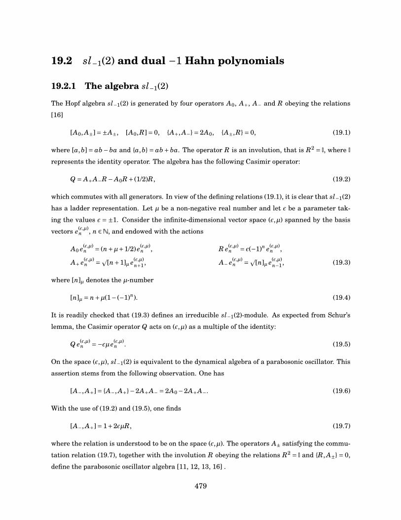
19.2 sl−1(2) and dual −1 Hahn polynomials
19.2.1 The algebra sl−1(2)
The Hopf algebra sl−1(2) is generated by four operators A0, A+, A− and R obeying the relations
[16]
[A0, A±]=±A±, [A0,R]= 0, A+, A−= 2A0, A±,R= 0, (19.1)
where [a,b] = ab− ba and a,b = ab+ ba. The operator R is an involution, that is R2 = I, where I
represents the identity operator. The algebra has the following Casimir operator:
Q = A+A−R− A0R+ (1/2)R, (19.2)
which commutes with all generators. In view of the defining relations (19.1), it is clear that sl−1(2)
has a ladder representation. Let µ be a non-negative real number and let ε be a parameter tak-
ing the values ε = ±1. Consider the infinite-dimensional vector space (ε,µ) spanned by the basis
vectors e(ε,µ)n , n ∈N, and endowed with the actions
A0 e(ε,µ)n = (n+µ+1/2) e(ε,µ)
n , R e(ε,µ)n = ε(−1)n e(ε,µ)
n ,
A+ e(ε,µ)n =p
[n+1]µ e(ε,µ)n+1 , A− e(ε,µ)
n =p[n]µ e(ε,µ)
n−1 , (19.3)
where [n]µ denotes the µ-number
[n]µ = n+µ(1− (−1)n). (19.4)
It is readily checked that (19.3) defines an irreducible sl−1(2)-module. As expected from Schur’s
lemma, the Casimir operator Q acts on (ε,µ) as a multiple of the identity:
Q e(ε,µ)n =−εµ e(ε,µ)
n . (19.5)
On the space (ε,µ), sl−1(2) is equivalent to the dynamical algebra of a parabosonic oscillator. This
assertion stems from the following observation. One has
[A−, A+]= A−, A+−2A+A− = 2A0 −2A+A−. (19.6)
With the use of (19.2) and (19.5), one finds
[A−, A+]= 1+2εµR, (19.7)
where the relation is understood to be on the space (ε,µ). The operators A± satisfying the commu-
tation relation (19.7), together with the involution R obeying the relations R2 = I and R, A± = 0,
define the parabosonic oscillator algebra [11, 12, 13, 16] .
479
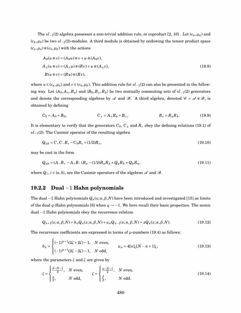
The sl−1(2) algebra possesses a non-trivial addition rule, or coproduct [2, 16] . Let (εa,µa) and
(εb,µb) be two sl−1(2)-modules. A third module is obtained by endowing the tensor product space
(εa,µa)⊗ (εb,µb) with the actions
A0(u⊗v)= (A0u)⊗v+u⊗ (A0v),
A±(u⊗v)= (A±u)⊗ (Rv)+u⊗ (A±v), (19.8)
R(u⊗v)= (Ru)⊗ (Rv),
where u ∈ (εa,µa) and v ∈ (εb,µb). This addition rule for sl−1(2) can also be presented in the follow-
ing way. Let A0, A±,Ra and B0,B±,Rb be two mutually commuting sets of sl−1(2) generators
and denote the corresponding algebras by A and B. A third algebra, denoted C = A ⊕B, is
obtained by defining
C0 = A0 +B0, C± = A±Rb +B±, Rc = RaRb. (19.9)
It is elementary to verify that the generators C0, C± and Rc obey the defining relations (19.1) of
sl−1(2). The Casimir operator of the resulting algebra
Qab = C+C−Rc −C0Rc + (1/2)Rc, (19.10)
may be cast in the form
Qab = (A−B+− A+B−)Ra − (1/2)RaRb +QaRb +QbRa, (19.11)
where Q i, i ∈ a,b, are the Casimir operators of the algebras A and B.
19.2.2 Dual −1 Hahn polynomials
The dual −1 Hahn polynomials Qn(x;α,β, N) have been introduced and investigated [15] as limits
of the dual q-Hahn polynomials [8] when q →−1. We here recall their basic properties. The monic
dual −1 Hahn polynomials obey the recurrence relation
Qn+1(x;α,β, N)+bnQn(x;α,β, N)+unQn−1(x;α,β, N)= xQn(x;α,β, N). (19.12)
The recurrence coefficients are expressed in terms of µ-numbers (19.4) as follows:
bn =
(−1)n+1(2ξ+2ζ)−1, N even,
(−1)n+1(2ξ−2ζ)−1, N odd,un = 4[n]ξ[N −n+1]ζ, (19.13)
where the parameters ξ and ζ are given by
ξ=
β−N−1
2 , N even,
α2 , N odd,
ζ=
α−N−1
2 , N even,β2 , N odd.
(19.14)
480

It is seen that the truncation conditions u0 = 0 and uN+1 = 0, necessary for finite orthogonal poly-
nomials, are met. The positivity condition un > 0 is equivalent to the condition α > N and β > N
in the case of even N. When N is odd, two conditions are possible to ensure positivity; the rele-
vant situation here is α>−1 and β>−1. The dual −1 Hahn polynomials enjoy the orthogonality
relationN∑
s=0ωsQn(xs;α,β, N)Qm(xs;α,β, N)= vnδnm. (19.15)
The grid and weight function are given by
xs =
(−1)s(2s+1−α−β), N even,
(−1)s(2s+1+α+β), N odd,(19.16)
ω2 j+q =
(−1) j (−N/2) j+qj!
(1−α/2) j(1−α/2−β/2) j(1−β/2) j(N/2+1−α/2−β/2) j+q
, N even,
(−1) j (−(N−1)/2) jj!
(1/2+α/2) j+q(1+α/2+β/2) j(1/2+β/2) j+q(N/2+3/2+α/2+β/2) j
, N odd,(19.17)
where q ∈ 0,1 and where (a)n = (a)(a+1) · · · (a+ n−1) stands for the Pochhammer symbol. The
normalization coefficients vn take the form
vn =
(−1)q(16)2 j+q j!(1−α/2) j(−N/2) j+q(β/2−N/2) j+q
((1−(α+β)/2)N/2
(1−β/2)N/2
), N even,
(−1)q(16)2 j+q j!(1/2+α/2) j+q(1/2−N/2) j(−β/2−N/2) j+q
((1+(α+β)/2)dN/2e
((β+1)/2)dN/2e
), N odd,
(19.18)
where dxe = bxc+1 and bxc denotes the integer part of x. The dual −1 Hahn polynomi-
als admit a hypergeometric representation. Recall that the generalized hypergeometric
function pFq(z) is defined by the infinite series
pFq
[a1 · · · ap
b1 · · · bq; z
]=∑
k
(a1)k · · · (ap)k
(b1)k · · · (bq)k
zk
k!. (19.19)
When N is even, one has [15]
Q2n(x)= γ(0)n 3F2
[−n,δ+ x+14 ,δ− x+1
4
−N2 ,1− α
2
;1], δ= 1/2− α+β
4, (19.20)
Q2n+1(x)= γ(1)n (x+1−τ)3F2
[−n,δ+ x+14 ,δ− x+1
4
1− N2 ,1− α
2
;1], τ= 2N +2−α−β, (19.21)
where γ(0)n = 16n(−N/2)n(1−α/2)n and γ(1)
n = 16n(1−N/2)n(1−α/2)n. When N is odd, one
rather has
Q2n(x)=φ(0)n 3F2
[−n,η+ x+14 ,η− x+1
41−N
2 , α+12
;1], η= α+β+2
4, (19.22)
Q2n+1(x)=φ(1)n (x+1+α−β)3F2
[−n,η+ x+14 ,η− x+1
41−N
2 , α+32
;1], (19.23)
481
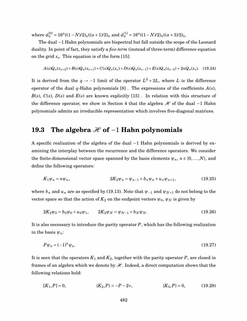
where φ(0)n = 16n((1−N)/2)n((α+1)/2)n and φ(1)
n = 16n((1−N)/2)n((α+3)/2)n.
The dual −1 Hahn polynomials are bispectral but fall outside the scope of the Leonardduality. In point of fact, they satisfy a five-term (instead of three-term) difference equationon the grid xs. This equation is of the form [15]:
A(s)Qn(xs+2)+B(s)Qn(xs+1)+C(s)Qn(xs)+D(s)Qn(xs−1)+E(s)Qn(xs−2)= 2nQn(xs). (19.24)
It is derived from the q → −1 limit of the operator L2 + 2L, where L is the difference
operator of the dual q-Hahn polynomials [8] . The expressions of the coefficients A(s),
B(s), C(s), D(s) and E(s) are known explicitly [15] . In relation with this structure of
the difference operator, we show in Section 4 that the algebra H of the dual −1 Hahn
polynomials admits an irreducible representation which involves five-diagonal matrices.
19.3 The algebra H of −1 Hahn polynomials
A specific realization of the algebra of the dual −1 Hahn polynomials is derived by ex-
amining the interplay between the recurrence and the difference operators. We consider
the finite-dimensional vector space spanned by the basis elements ψn, n ∈ 0, . . . , N, and
define the following operators:
K1ψn = nψn, 2K2ψn =ψn−1 +bnψn +unψn+1, (19.25)
where bn and un are as specified by (19.13). Note that ψ−1 and ψN+1 do not belong to the
vector space so that the action of K2 on the endpoint vectors ψ0, ψN is given by
2K2ψ0 = b0ψ0 +u0ψ1, 2K2ψN =ψN−1 +bNψN . (19.26)
It is also necessary to introduce the parity operator P, which has the following realization
in the basis ψn:
Pψn = (−1)nψn. (19.27)
It is seen that the operators K1 and K2, together with the parity operator P, are closed in
frames of an algebra which we denote by H . Indeed, a direct computation shows that the
following relations hold:
[K1,P]= 0, K2,P=−P −2ν, K3,P= 0, (19.28)
482
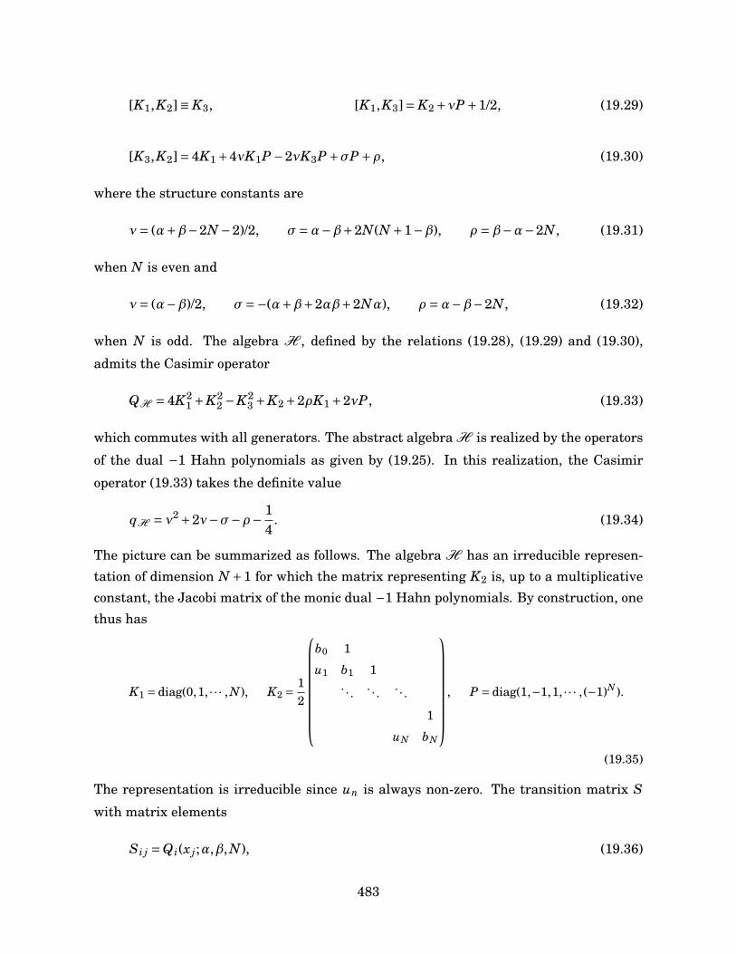
[K1,K2]≡ K3, [K1,K3]= K2 +νP +1/2, (19.29)
[K3,K2]= 4K1 +4νK1P −2νK3P +σP +ρ, (19.30)
where the structure constants are
ν= (α+β−2N −2)/2, σ=α−β+2N(N +1−β), ρ =β−α−2N, (19.31)
when N is even and
ν= (α−β)/2, σ=−(α+β+2αβ+2Nα), ρ =α−β−2N, (19.32)
when N is odd. The algebra H , defined by the relations (19.28), (19.29) and (19.30),
admits the Casimir operator
QH = 4K21 +K2
2 −K23 +K2 +2ρK1 +2νP, (19.33)
which commutes with all generators. The abstract algebra H is realized by the operators
of the dual −1 Hahn polynomials as given by (19.25). In this realization, the Casimir
operator (19.33) takes the definite value
qH = ν2 +2ν−σ−ρ− 14
. (19.34)
The picture can be summarized as follows. The algebra H has an irreducible represen-tation of dimension N +1 for which the matrix representing K2 is, up to a multiplicativeconstant, the Jacobi matrix of the monic dual −1 Hahn polynomials. By construction, onethus has
K1 = diag(0,1, · · · , N), K2 = 12
b0 1
u1 b1 1. . . . . . . . .
1
uN bN
, P = diag(1,−1,1, · · · , (−1)N ).
(19.35)
The representation is irreducible since un is always non-zero. The transition matrix S
with matrix elements
Si j =Q i(x j;α,β, N), (19.36)
483
in the ψn basis provides the similarity transformation diagonalizing K2. Equivalently,
the dual −1 Hahn polynomials are, up to factors, the overlap coefficients of the bases in
which either K1 or K2 is diagonal. It is clear that in the basis in which K2 is diagonal,
the operators P and K1 will not be diagonal. In Section 4, the matrix elements of P and
K1 in this basis will be constructed from the commutation relations (19.28), (19.29) and
(19.30). Unsurprisingly, the operator K1 will be shown to be five-diagonal in this basis as
expected from the form of the difference equation. We now turn to the Clebsch-Gordan
problem.
19.4 The Clebsch-Gordan problem
The Clebsch-Gordan problem for sl−1(2) can be posited in the following way. We consider
the sl−1(2)-module (εa,µa)⊗ (εb,µb) that we wish to decompose irreducibly. The basis vec-
tors e(εa,µa)na ⊗e(εb,µb)
nb of the direct product are characterized as eigenvectors of the operators
Qa, A0, Ra, Qb, B0, Rb, (19.37)
with eigenvalues
−εaµa, na +µa +1/2, (−1)naεa, −εbµb, nb +µb +1/2, (−1)nbεb, (19.38)
respectively. The irreducible modules in the decomposition will be spanned by the ele-
ments e(εab,µab)k refered to as the coupled basis vectors. In each irreducible component, the
(total) Casimir operator Qab of the two added sl−1(2) algebras which reads
Qab = (A−B+− A+B−)Ra − (1/2)RaRb +QaRb +QbRa, (19.39)
acts as a multiple of the identity:
Qab =−εabµab I. (19.40)
The coupled basis elements e(εab,µab)k are the eigenvectors of
Qab, RaRb, Qa, Qb, A0 +B0, (19.41)
with eigenvalues
−εabµab, εab, −εaµa, −εbµb, k+µa +µb +1, (19.42)
484
respectively. The direct product basis is related to the coupled basis by a unitary trans-
formation whose matrix elements are called Clebsch-Gordan coefficients. These overlap
coefficients will be zero unless
k = na +nb ≡ N. (19.43)
We may hence write
e(εab,µab)N = ∑
na+nb=NCµaµbµab
nanbN e(εaµa)na ⊗ e(εbµb)
nb , (19.44)
where CµaµbµabnanbN are the Clebsch-Gordan coefficients of sl−1(2).
The Clebsch-Gordan problem for sl−1(2) can be solved elegantly by examining the un-
derlying symmetry algebra. It is first observed that for a given N, the following operators
act as multiples of the identity operator on both sides of (19.44):
Λ1 = 2Qa, Λ2 = 2Qb, Λ3 = RaRb, Λ4 = A0 +B0, (19.45)
with multiples
λ1 =−2εaµa, λ2 =−2εbµb, λ3 = (−1)Nεaεb, λ4 =µa +µb +N +1. (19.46)
Let us now introduce the following operators
κ1 = (A0 −B0)/2, κ2 =Λ3Qab, r = Ra. (19.47)
The Clebsch-Gordan problem for sl−1(2) is tantamount to finding the overlaps between
the eigenvectors of κ1 and r and the eigenvectors of κ2. The first set of eigenvectors
correspond to the elements of the direct product basis (R.H.S. of (19.44)) since κ1 and r
complement the set (19.45) to give all the labelling operators (19.37). The second set is
identified as should be to the coupled basis elements (L.H.S. of (19.44)) since only Qab
needs to be added to (19.45) to recover the complete set of operators (19.41) that are
diagonal on the coupled vectors e(εab,µab)N ; it will prove convenient to use equivalently κ2 =
Λ3Qab, instead of Qab.
Let us now consider the algebra which is generated by these operators, i.e. by κ1, κ2
and r. Let κ3 be a fourth generator defined by
κ3 ≡ [κ1,κ2]. (19.48)
485
A direct computation shows that:
[κ1, r]= 0, κ2, r=−r+ (λ1 +λ2λ3), κ3, r= 0, (19.49)
[κ1,κ3]= κ2 − 12
(λ1 +λ2λ3)r+1/2, (19.50)
[κ3,κ2]= 4κ1 + (λ1 +λ2λ3)κ3r−2(λ1 +λ2λ3)κ1r+λ4(λ1 −λ2λ3)r. (19.51)
In this instance the Casimir operator for the algebra is given by
QC.G. = 4κ21 +κ2
2 −κ23 +κ2 − (λ1 +λ2λ3)r, (19.52)
and acts as a multiple qC.G. of the identity:
qC.G. =14
(λ1 +λ2λ3)2 +λ24 −
54
. (19.53)
It is seen that the algebra H of the dual −1 Hahn polynomials arises as the hidden
symmetry algebra of the Clebsch-Gordan problem of sl−1(2). Indeed, redefining K1 →K1 +ρ/4 in (19.28), (19.29) and (19.30) yields an algebra of the form (19.49), (19.50) and
(19.51).
In order to establish the exact correspondence between the Clebsch-Gordan coeffi-
cients of sl−1(2) and the dual −1 Hahn polynomials encompassed by the algebra, it is
necessary to determine the spectra of the operators κ1 and κ2. In view of the action of A0
in (19.3), it is clear that κ1 = (A0 −B0)/2 has a linear spectrum of the form
λκ1 = n+ (µa −µb −N)/2, n ∈ 0, · · · , N. (19.54)
This spectrum is seen to coincide, up to a translation, with that of operator K1 in the
algebra H of the dual −1 Hahn polynomials.
The evaluation of the spectrum of Qab is more delicate. In a given sl−1(2)-module
(ε,µ), it follows from (19.3) and (19.5) that the eigenvalues of A0 are given by
λA0 = n−εQ+1/2. (19.55)
In reducible representations, it is hence possible from this relation to determine the eigen-
values of the Casimir operator which are compatible with the eigenvalue λA0 of A0 that
is being considered. So, for a given λA0 , the absolute value |q| of the possible eigenvalues
q of the Casimir operator are
|q| = |λA0 −1/2|, |λA0 −3/2|, . . . , (19.56)
486
In the calculation of the Clebsch-Gordan coefficients of sl−1(2), the eigenvalue of C0 =A0 +B0 is taken to be µa +µb +N +1. Consequently, the set of the absolute values of the
possible eigenvalues of Qc =Qab given in (19.39) is of cardinality N +1 and is found to be
|qab| =µa +µb +N +1/2,µa +µb +N −1/2, · · · ,µa +µb +1/2. (19.57)
Since the eigenvalue of Qab is −εabµab, it follows that the admissible values of µab are
given by the above ensemble (19.57) with µab = |qab|.There remains to evaluate the associated values of εab. To that end, consider the eigen-
vector e0 = e(εab|max,µab|max)N of the coupled basis corresponding to the maximal admissible
value of µab. The state e0 satisfies the relations
C0 e0 = (µa +µb +N +1)e0, C− e0 = 0. (19.58)
On the one hand, it then follows from (19.58) and (19.3) that
Rc e0 = εab|max e0. (19.59)
On the other hand, the value of Rc = RaRb is fixed to be (−1)Nεaεb on the whole space so
that in particular Rc e0 = (−1)Nεaεb e0. We therefore conclude that for the state with the
maximal value µab =µab|max of µab, the corresponding value εab|max of εab is
εab|max = (−1)Nεaεb. (19.60)
Since Qab e0 = Qabe(εab|max,µab|max)N = −εab|maxµab|max, it follows that this eigenvalue qab of
the full Casimir operator Qab is
qab = (−1)N+1εaεb(µa +µb +N +1/2). (19.61)
It is easily seen that incrementing the projection from N to N +1 adds a new eigenvalue
to the set of eigenvalues of Qab while preserving the admissible values of (εab,µab) for the
original value N of the projection. Thus, by induction, the eigenvalues of the full Casimir
operator Qc =Qab are given by
qab =−εabµab = (−1)s+1εaεb(µa +µb + s+1/2), s = 0, . . . , N. (19.62)
It is thus seen that the spectrum of κ2 coincide with that of K2 in the algebra H and that
the Clebsch-Gordan coefficients of sl−1(2) are hence proportional to the dual −1 Hahn
polynomials.
487
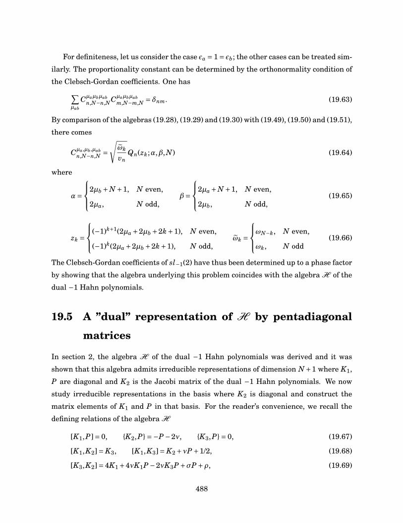
For definiteness, let us consider the case εa = 1= εb; the other cases can be treated sim-
ilarly. The proportionality constant can be determined by the orthonormality condition of
the Clebsch-Gordan coefficients. One has∑µab
Cµaµbµabn,N−n,NCµaµbµab
m,N−m,N = δnm. (19.63)
By comparison of the algebras (19.28), (19.29) and (19.30) with (19.49), (19.50) and (19.51),
there comes
Cµa,µb,µabn,N−n,N =
√ωk
vnQn(zk;α,β, N) (19.64)
where
α=
2µb +N +1, N even,
2µa, N odd,β=
2µa +N +1, N even,
2µb, N odd,(19.65)
zk =
(−1)k+1(2µa +2µb +2k+1), N even,
(−1)k(2µa +2µb +2k+1), N odd,ωk =
ωN−k, N even,
ωk, N odd(19.66)
The Clebsch-Gordan coefficients of sl−1(2) have thus been determined up to a phase factor
by showing that the algebra underlying this problem coincides with the algebra H of the
dual −1 Hahn polynomials.
19.5 A ”dual” representation of H by pentadiagonal
matrices
In section 2, the algebra H of the dual −1 Hahn polynomials was derived and it was
shown that this algebra admits irreducible representations of dimension N+1 where K1,
P are diagonal and K2 is the Jacobi matrix of the dual −1 Hahn polynomials. We now
study irreducible representations in the basis where K2 is diagonal and construct the
matrix elements of K1 and P in that basis. For the reader’s convenience, we recall the
defining relations of the algebra H
[K1,P]= 0, K2,P=−P −2ν, K3,P= 0, (19.67)
[K1,K2]= K3, [K1,K3]= K2 +νP +1/2, (19.68)
[K3,K2]= 4K1 +4νK1P −2νK3P +σP +ρ, (19.69)
488
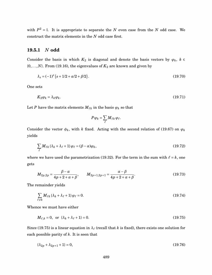
with P2 = I. It is appropriate to separate the N even case from the N odd case. We
construct the matrix elements in the N odd case first.
19.5.1 N odd
Consider the basis in which K2 is diagonal and denote the basis vectors by ϕk, k ∈0, . . . , N. From (19.16), the eigenvalues of K2 are known and given by
λs = (−1)s (s+1/2+α/2+β/2
). (19.70)
One sets
K2ϕk =λkϕk. (19.71)
Let P have the matrix elements M`k in the basis ϕk so that
Pϕk =∑`
M`kϕ`.
Consider the vector φk, with k fixed. Acting with the second relation of (19.67) on ϕk
yields∑`
M`k λk +λ`+1ϕ` = (β−α)ϕk, (19.72)
where we have used the parametrization (19.32). For the term in the sum with `= k, one
gets
M2p,2p = β−α4p+2+α+β , M2p+1,2p+1 = α−β
4p+2+α+β . (19.73)
The remainder yields∑` 6=k
M`k λk +λ`+1ϕ` = 0. (19.74)
Whence we must have either
M`,k = 0, or λk +λ`+1= 0. (19.75)
Since (19.75) is a linear equation in λ` (recall that k is fixed), there exists one solution for
each possible parity of k. It is seen that
λ2p +λ2p+1 +1= 0, (19.76)
489
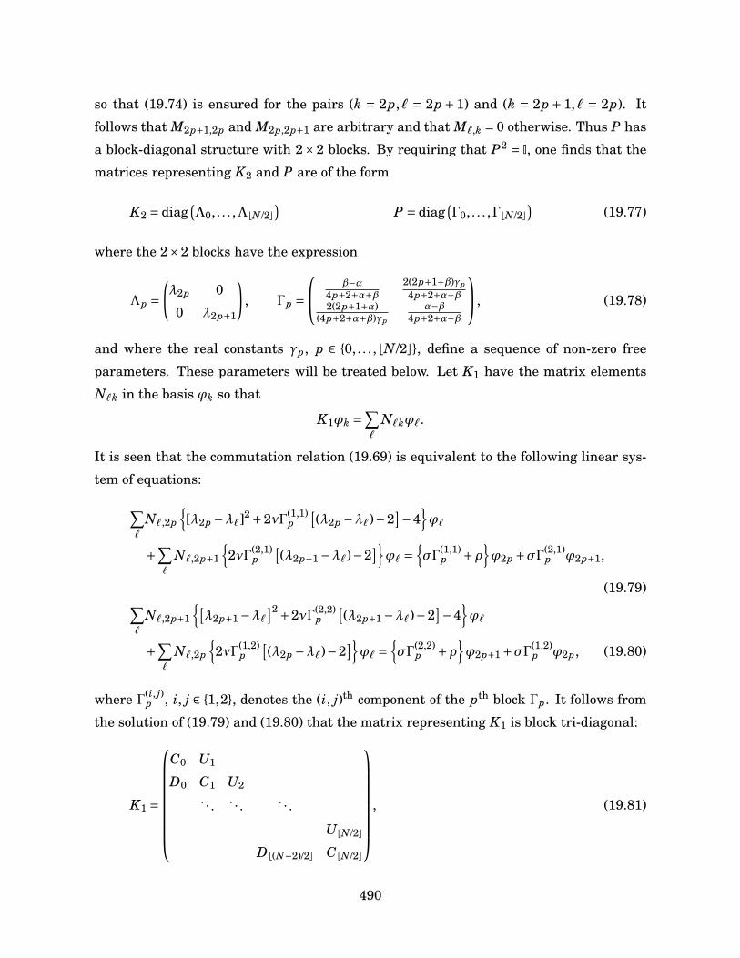
so that (19.74) is ensured for the pairs (k = 2p,` = 2p + 1) and (k = 2p + 1,` = 2p). It
follows that M2p+1,2p and M2p,2p+1 are arbitrary and that M`,k = 0 otherwise. Thus P has
a block-diagonal structure with 2×2 blocks. By requiring that P2 = I, one finds that the
matrices representing K2 and P are of the form
K2 = diag(Λ0, . . . ,ΛbN/2c
)P = diag
(Γ0, . . . ,ΓbN/2c
)(19.77)
where the 2×2 blocks have the expression
Λp =(λ2p 0
0 λ2p+1
), Γp =
β−α4p+2+α+β
2(2p+1+β)γp4p+2+α+β
2(2p+1+α)(4p+2+α+β)γp
α−β4p+2+α+β
, (19.78)
and where the real constants γp, p ∈ 0, . . . ,bN/2c, define a sequence of non-zero free
parameters. These parameters will be treated below. Let K1 have the matrix elements
N`k in the basis ϕk so that
K1ϕk =∑`
N`kϕ`.
It is seen that the commutation relation (19.69) is equivalent to the following linear sys-
tem of equations:
∑`
N`,2p
[λ2p −λ`]2 +2νΓ(1,1)
p[(λ2p −λ`)−2
]−4ϕ`
+∑`
N`,2p+1
2νΓ(2,1)
p[(λ2p+1 −λ`)−2
]ϕ` =
σΓ
(1,1)p +ρ
ϕ2p +σΓ(2,1)
p ϕ2p+1,
(19.79)∑`
N`,2p+1
[λ2p+1 −λ`
]2 +2νΓ(2,2)p
[(λ2p+1 −λ`)−2
]−4ϕ`
+∑`
N`,2p
2νΓ(1,2)
p[(λ2p −λ`)−2
]ϕ` =
σΓ
(2,2)p +ρ
ϕ2p+1 +σΓ(1,2)
p ϕ2p, (19.80)
where Γ(i, j)p , i, j ∈ 1,2, denotes the (i, j)th component of the pth block Γp. It follows from
the solution of (19.79) and (19.80) that the matrix representing K1 is block tri-diagonal:
K1 =
C0 U1
D0 C1 U2. . . . . . . . .
UbN/2cDb(N−2)/2c CbN/2c
, (19.81)
490
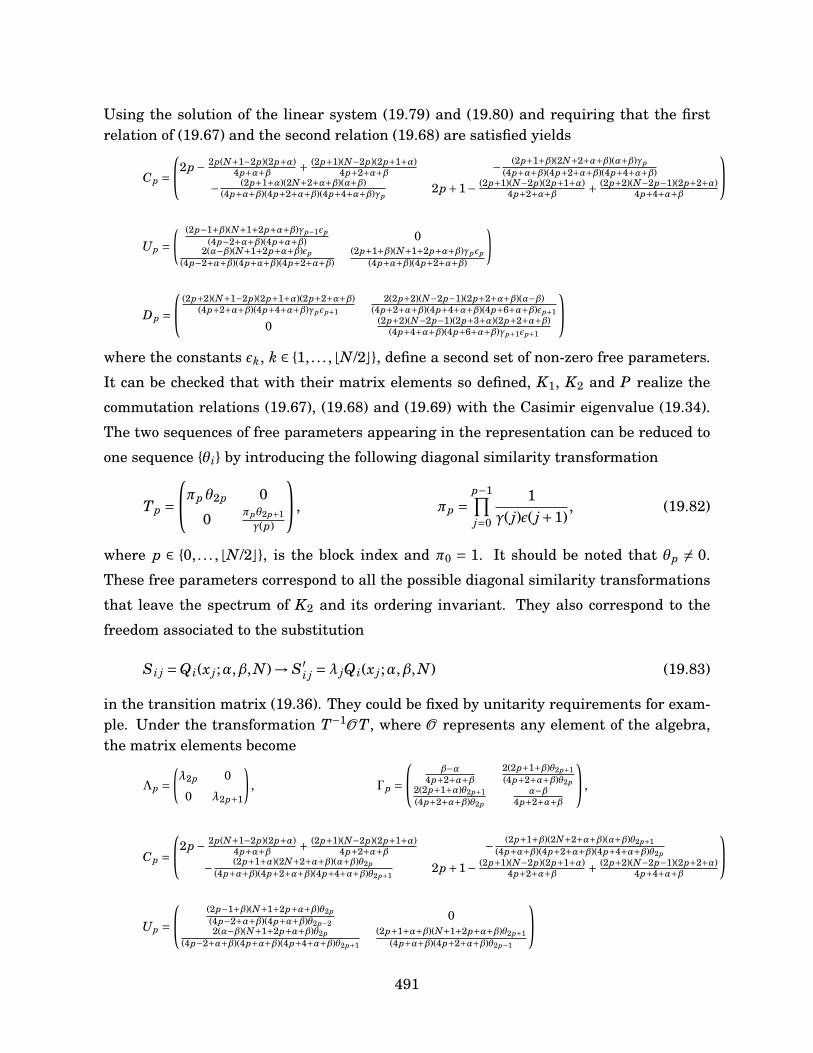
Using the solution of the linear system (19.79) and (19.80) and requiring that the firstrelation of (19.67) and the second relation (19.68) are satisfied yields
Cp =2p− 2p(N+1−2p)(2p+α)
4p+α+β + (2p+1)(N−2p)(2p+1+α)4p+2+α+β − (2p+1+β)(2N+2+α+β)(α+β)γp
(4p+α+β)(4p+2+α+β)(4p+4+α+β)
− (2p+1+α)(2N+2+α+β)(α+β)(4p+α+β)(4p+2+α+β)(4p+4+α+β)γp
2p+1− (2p+1)(N−2p)(2p+1+α)4p+2+α+β + (2p+2)(N−2p−1)(2p+2+α)
4p+4+α+β
Up =( (2p−1+β)(N+1+2p+α+β)γp−1εp
(4p−2+α+β)(4p+α+β) 02(α−β)(N+1+2p+α+β)εp
(4p−2+α+β)(4p+α+β)(4p+2+α+β)(2p+1+β)(N+1+2p+α+β)γpεp
(4p+α+β)(4p+2+α+β)
)
Dp = (2p+2)(N+1−2p)(2p+1+α)(2p+2+α+β)
(4p+2+α+β)(4p+4+α+β)γpεp+1
2(2p+2)(N−2p−1)(2p+2+α+β)(α−β)(4p+2+α+β)(4p+4+α+β)(4p+6+α+β)εp+1
0 (2p+2)(N−2p−1)(2p+3+α)(2p+2+α+β)(4p+4+α+β)(4p+6+α+β)γp+1εp+1
where the constants εk, k ∈ 1, . . . ,bN/2c, define a second set of non-zero free parameters.
It can be checked that with their matrix elements so defined, K1, K2 and P realize the
commutation relations (19.67), (19.68) and (19.69) with the Casimir eigenvalue (19.34).
The two sequences of free parameters appearing in the representation can be reduced to
one sequence θi by introducing the following diagonal similarity transformation
Tp =πp θ2p 0
0 πpθ2p+1γ(p)
, πp =p−1∏j=0
1γ( j)ε( j+1)
, (19.82)
where p ∈ 0, . . . ,bN/2c, is the block index and π0 = 1. It should be noted that θp 6= 0.
These free parameters correspond to all the possible diagonal similarity transformations
that leave the spectrum of K2 and its ordering invariant. They also correspond to the
freedom associated to the substitution
Si j =Q i(x j;α,β, N)→ S′i j =λ jQ i(x j;α,β, N) (19.83)
in the transition matrix (19.36). They could be fixed by unitarity requirements for exam-ple. Under the transformation T−1OT, where O represents any element of the algebra,the matrix elements become
Λp =(λ2p 0
0 λ2p+1
), Γp =
β−α4p+2+α+β
2(2p+1+β)θ2p+1(4p+2+α+β)θ2p
2(2p+1+α)θ2p+1(4p+2+α+β)θ2p
α−β4p+2+α+β
,
Cp =2p− 2p(N+1−2p)(2p+α)
4p+α+β + (2p+1)(N−2p)(2p+1+α)4p+2+α+β − (2p+1+β)(2N+2+α+β)(α+β)θ2p+1
(4p+α+β)(4p+2+α+β)(4p+4+α+β)θ2p
− (2p+1+α)(2N+2+α+β)(α+β)θ2p(4p+α+β)(4p+2+α+β)(4p+4+α+β)θ2p+1
2p+1− (2p+1)(N−2p)(2p+1+α)4p+2+α+β + (2p+2)(N−2p−1)(2p+2+α)
4p+4+α+β
Up = (2p−1+β)(N+1+2p+α+β)θ2p
(4p−2+α+β)(4p+α+β)θ2p−20
2(α−β)(N+1+2p+α+β)θ2p(4p−2+α+β)(4p+α+β)(4p+4+α+β)θ2p+1
(2p+1+α+β)(N+1+2p+α+β)θ2p+1(4p+α+β)(4p+2+α+β)θ2p−1
491
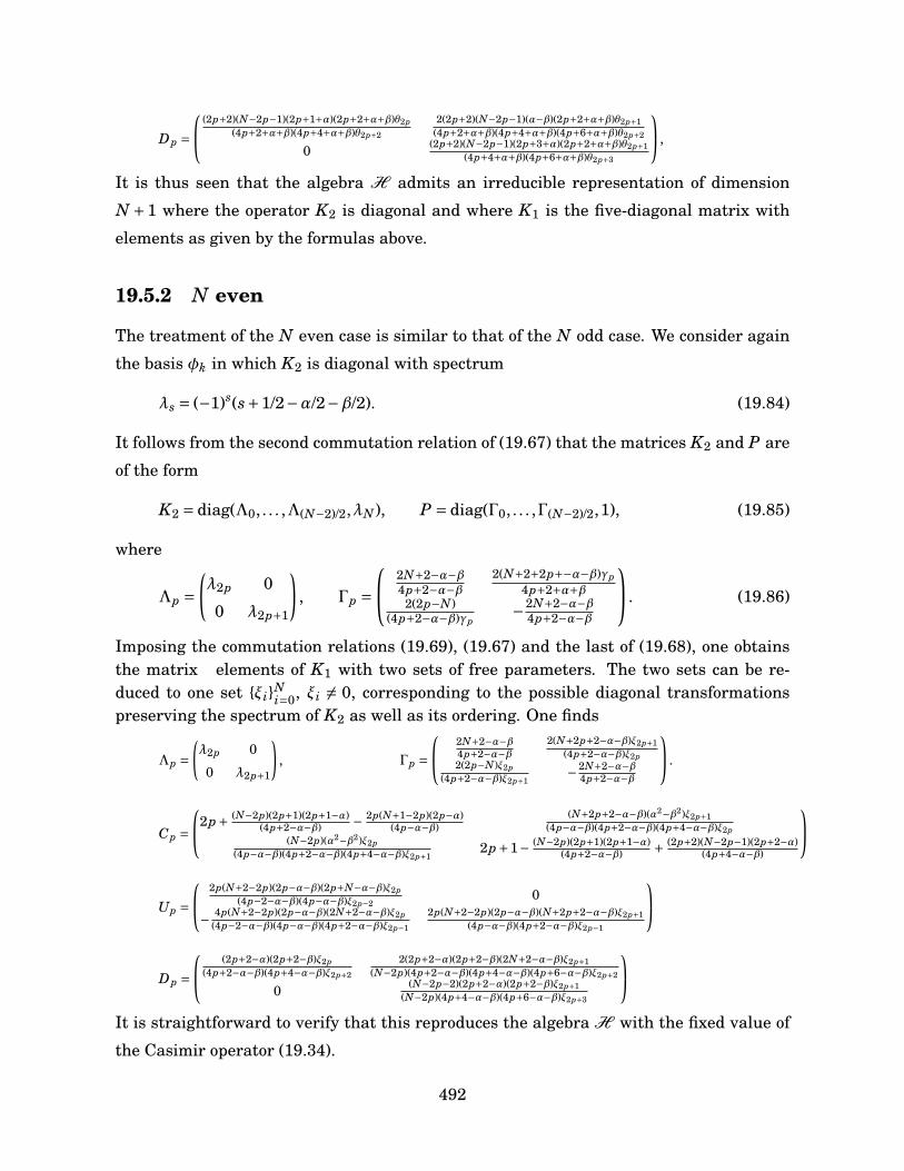
Dp = (2p+2)(N−2p−1)(2p+1+α)(2p+2+α+β)θ2p
(4p+2+α+β)(4p+4+α+β)θ2p+2
2(2p+2)(N−2p−1)(α−β)(2p+2+α+β)θ2p+1(4p+2+α+β)(4p+4+α+β)(4p+6+α+β)θ2p+2
0 (2p+2)(N−2p−1)(2p+3+α)(2p+2+α+β)θ2p+1(4p+4+α+β)(4p+6+α+β)θ2p+3
,
It is thus seen that the algebra H admits an irreducible representation of dimension
N +1 where the operator K2 is diagonal and where K1 is the five-diagonal matrix with
elements as given by the formulas above.
19.5.2 N even
The treatment of the N even case is similar to that of the N odd case. We consider again
the basis φk in which K2 is diagonal with spectrum
λs = (−1)s(s+1/2−α/2−β/2). (19.84)
It follows from the second commutation relation of (19.67) that the matrices K2 and P are
of the form
K2 = diag(Λ0, . . . ,Λ(N−2)/2,λN), P = diag(Γ0, . . . ,Γ(N−2)/2,1), (19.85)
where
Λp =(λ2p 0
0 λ2p+1
), Γp =
2N+2−α−β4p+2−α−β
2(N+2+2p+−α−β)γp4p+2+α+β
2(2p−N)(4p+2−α−β)γp
−2N+2−α−β4p+2−α−β
. (19.86)
Imposing the commutation relations (19.69), (19.67) and the last of (19.68), one obtainsthe matrix elements of K1 with two sets of free parameters. The two sets can be re-duced to one set ξiN
i=0, ξi 6= 0, corresponding to the possible diagonal transformationspreserving the spectrum of K2 as well as its ordering. One finds
Λp =(λ2p 0
0 λ2p+1
), Γp =
2N+2−α−β4p+2−α−β
2(N+2p+2−α−β)ξ2p+1(4p+2−α−β)ξ2p
2(2p−N)ξ2p(4p+2−α−β)ξ2p+1
− 2N+2−α−β4p+2−α−β
.
Cp =2p+ (N−2p)(2p+1)(2p+1−α)
(4p+2−α−β) − 2p(N+1−2p)(2p−α)(4p−α−β)
(N+2p+2−α−β)(α2−β2)ξ2p+1(4p−α−β)(4p+2−α−β)(4p+4−α−β)ξ2p
(N−2p)(α2−β2)ξ2p(4p−α−β)(4p+2−α−β)(4p+4−α−β)ξ2p+1
2p+1− (N−2p)(2p+1)(2p+1−α)(4p+2−α−β) + (2p+2)(N−2p−1)(2p+2−α)
(4p+4−α−β)
Up = 2p(N+2−2p)(2p−α−β)(2p+N−α−β)ξ2p
(4p−2−α−β)(4p−α−β)ξ2p−20
− 4p(N+2−2p)(2p−α−β)(2N+2−α−β)ξ2p(4p−2−α−β)(4p−α−β)(4p+2−α−β)ξ2p−1
2p(N+2−2p)(2p−α−β)(N+2p+2−α−β)ξ2p+1(4p−α−β)(4p+2−α−β)ξ2p−1
Dp = (2p+2−α)(2p+2−β)ξ2p
(4p+2−α−β)(4p+4−α−β)ξ2p+2
2(2p+2−α)(2p+2−β)(2N+2−α−β)ξ2p+1(N−2p)(4p+2−α−β)(4p+4−α−β)(4p+6−α−β)ξ2p+2
0 (N−2p−2)(2p+2−α)(2p+2−β)ξ2p+1(N−2p)(4p+4−α−β)(4p+6−α−β)ξ2p+3
It is straightforward to verify that this reproduces the algebra H with the fixed value of
the Casimir operator (19.34).
492
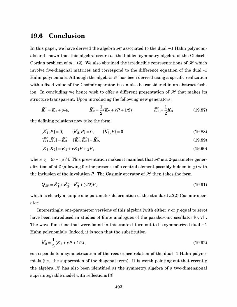
19.6 Conclusion
In this paper, we have derived the algebra H associated to the dual −1 Hahn polynomi-
als and shown that this algebra occurs as the hidden symmetry algebra of the Clebsch-
Gordan problem of sl−1(2). We also obtained the irreducible representations of H which
involve five-diagonal matrices and correspond to the difference equation of the dual -1
Hahn polynomials. Although the algebra H has been derived using a specific realization
with a fixed value of the Casimir operator, it can also be considered in an abstract fash-
ion. In concluding we hence wish to offer a different presentation of H that makes its
structure transparent. Upon introducing the following new generators:
K1 = K1 +ρ/4, K2 = 12
(K2 +νP +1/2) , K3 = 12
K3 (19.87)
the defining relations now take the form:
[K1,P]= 0, K2,P= 0, K3,P= 0 (19.88)
[K1, K2]= K3, [K1, K3]= K2, (19.89)
[K3, K2]= K1 +νK1P +χP, (19.90)
where χ= (σ−νρ)/4. This presentation makes it manifest that H is a 2-parameter gener-
alization of u(2) (allowing for the presence of a central element possibly hidden in χ) with
the inclusion of the involution P. The Casimir operator of H then takes the form
QH = K21 + K2
2 − K23 + (ν/2)P, (19.91)
which is clearly a simple one-parameter deformation of the standard sl(2) Casimir oper-
ator.
Interestingly, one-parameter versions of this algebra (with either ν or χ equal to zero)
have been introduced in studies of finite analogues of the parabosonic oscillator [6, 7] .
The wave functions that were found in this context turn out to be symmetrized dual −1
Hahn polynomials. Indeed, it is seen that the substitution
K2 = 12
(K2 +νP +1/2) , (19.92)
corresponds to a symmetrization of the recurrence relation of the dual -1 Hahn polyno-
mials (i.e. the suppression of the diagonal term). It is worth pointing out that recently
the algebra H has also been identified as the symmetry algebra of a two-dimensional
superintegrable model with reflections [3].
493
The algebra H can be considered as an extension of the Askey-Wilson algebra AW(3)
[22] . It is known [9, 10] that these algebras are related to double-affine Hecke algebras
(DAHA). It would be of interest in the future to explore the possible relation between
DAHAs and the algebra H .
References[1] E. Bannai and T. Ito. Algebraic Combinatorics I: Associaion Schemes. Benjamin & Cummins,
1984.
[2] C. Daskaloyannis, K. Kanakoglou, and I. Tsohantjis. Hopf algebraic structure of the para-
bosonic and parafermionic algebras and paraparticle generelization of the Jordan-Schwinger
map. Journal of Mathematical Physics, 41, 2000.
[3] V.X. Genest, M.E.H. Ismail, L. Vinet, and A. Zhedanov. The Dunkl oscillator in the plane
I : superintegrability, separated wavefunctions and overlap coefficients . ArXiv:1212.4459,
2012.
[4] V.X. Genest, L. Vinet, and A. Zhedanov. Bispectrality of the Complementary Bannai-Ito
polynomials. ArXiv:1211.2461, 2012.
[5] H.S. Green. A generalized method of field quantization. Physical Review, 90, 1953.
[6] E.I. Jafarov, N.I. Stoilova, and J. Van der Jeugt. Finite oscillator models: the Hahn oscillator.
Journal of Physics A: Mathematical and General, 44, 2011.
[7] E.I. Jafarov, N.I. Stoilova, and J. Van der Jeugt. Deformed su(1,1) algebra as a model for
quantum oscillators. S.I.G.M.A., 8, 2012.
[8] R. Koekoek, P.A. Lesky, and R.F. Swarttouw. Hypergeometric orthogonal polynomials and
their q-analogues. Springer, 1st edition, 2010.
[9] T. Koornwinder. The Relationship between Zhedanov’s Algebra AW(3) and the Double Affine
Hecke Algebra in the Rank One Case . S.I.G.M.A., 3, 2007.
[10] T. Koornwinder. Zhedanov’s algebra AW(3) and the Double-Affine Hecke Algebra in the rank
one case II: The spherical subalgebra. S.I.G.M.A., 4, 2008.
[11] N. Mukunda, E.C.G. Sudarshan, J.K. Sharma, and C.L. Mehta. Representations and proper-
ties of para-Bose oscillator operators I: energy position and momentum eigenstates. Journal
of Mathematical Physics, 21, 1980.
494
[12] M. Rosenblum. Generalized Hermite polynomials and the Bose-like oscillator calculus. In
B. Sheva, editor, Non Self-Adjoint Operators and Related Topics, 1994.
[13] J.K. Sharma, C.L. Mehta, N. Mukunda, and E.C.G. Sudarshan. Representation and proper-
ties of para-Bose oscillator operators II: coherent states and the minimum uncertainty states.
Journal of Mathematical Physics, 22, 1981.
[14] P. Terwilliger. Two linear transformations each tridiagonal with respect to an eigenbasis of
the other. Linear Algebra and its Applications, 330, 2001.
[15] S. Tsujimoto, L. Vinet, and A. Zhedanov. Dual −1 Hahn polynomials: "classical" polynomials
beyond the Leonard duality. Proceedings of the American Mathematical Society, 2011.
[16] S. Tsujimoto, L. Vinet, and A. Zhedanov. From slq(2) to a Parabosonic Hopf Algebra.
S.I.G.M.A., 7, 2011.
[17] S. Tsujimoto, L. Vinet, and A. Zhedanov. Jordan algebras and orthogonal polynomials. Jour-
nal of Mathematical Physics, 52:103512, 2011.
[18] S. Tsujimoto, L. Vinet, and A. Zhedanov. Dunkl shift operators and Bannai-Ito polynomials.
Advances in Mathematics, 229:2123–2158, 2012.
[19] L. Vinet and A. Zhedanov. A Bochner theorem for Dunkl polynomials. S.I.G.M.A., 7, 2011.
[20] L. Vinet and A. Zhedanov. A limit q = −1 for big q-Jacobi polynomials. Transactions of the
American Mathematical Society, 2011.
[21] L. Vinet and A. Zhedanov. A "missing" family of classical orthogonal polynomials. Journal of
Physics A: Mathematical and General, 44, 2011.
[22] A. Zhedanov. Hidden symmetry of Askey-Wilson polynomials. Theoreticheskaya i Matem-
aticheskaya Fizika, 89, 1991.
495

496
Chapitre 20
The Bannai–Ito algebra and someapplications
H. De Bie, V. X. Genest, S. Tsujimoto, L. Vinet et A. Zhedanov (2015). The Bannai–Ito algebra and
some applications. Journal of Physics: Conference Series 597 012001
Abstract. The Bannai-Ito algebra is presented together with some of its applications. Its relations
with the Bannai-Ito polynomials, the Racah problem for the sl−1(2) algebra, a superintegrable
model with reflections and a Dirac-Dunkl equation on the 2-sphere are surveyed.
20.1 Introduction
Exploration through the exact solution of models has a secular tradition in mathematical physics.
Empirically, exact solvability is possible in the presence of symmetries, which come in various
guises and which are described by a variety of mathematical structures. In many cases, exact
solutions are expressed in terms of special functions, whose properties encode the symmetries of
the systems in which they arise. This can be represented by the following virtuous circle:
Exact solvability
Symmetriesxx
44
Special functions''
kk
Algebraic structuresss
77
**
ff
The classical path is the following: start with a model, find its symmetries, determine how these
symmetries are mathematically described, work out the representations of that mathematical
497
structure and obtain its relation to special functions to arrive at the solution of the model. How-
ever, one can profitably start from any node on this circle. For instance, one can identify and
characterize new special functions, determine the algebraic structure they encode, look for mod-
els that have this structure as symmetry algebra and proceed to the solution. In this paper, the
following path will be taken:
Algebra−→Orthogonal polynomials−→Symmetries−→Exact solutions
The outline of the paper is as follows. In section 2, the Bannai-Ito algebra is introduced and
some of its special cases are presented. In section 3, a realization of the Bannai-Ito algebra in
terms of discrete shift and reflection operators is exhibited. The Bannai-Ito polynomials and their
properties are discussed in section 4. In section 5, the Bannai-Ito algebra is used to derive the
recurrence relation satisfied by the Bannai-Ito polynomials. In section 6, the paraboson algebra
and the sl−1(2) algebra are introduced. In section 7, the realization of sl−1(2) in terms of Dunkl
operators is discussed. In section 8, the Racah problem for sl−1(2) and its relation with the Bannai-
Ito algebra is examined. A superintegrable model on the 2-sphere with Bannai-Ito symmetry
is studied in section 9. In section 10, a Dunkl-Dirac equation on the 2-sphere with Bannai-Ito
symmetry is discussed. A list of open questions is provided in lieu of a conclusion.
20.2 The Bannai-Ito algebra
Throughout the paper, the notation [A,B] = AB−BA and A,B = AB+BA will be used. Let ω1,
ω2 and ω3 be real parameters. The Bannai-Ito algebra is the associative algebra generated by K1,
K2 and K3 together with the three relations
K1,K2= K3 +ω3, K2,K3= K1 +ω1, K3,K1= K2 +ω2, (20.1)
or K i,K j= Kk +ωk, with (i jk) a cyclic permutation of (1,2,3). The Casimir operator
Q = K21 +K2
2 +K23 ,
commutes with every generator; this property is easily verified with the commutator identity
[AB,C] = AB,C− A,CB. Let us point out two special cases of (20.1) that have been considered
previously in the literature.
1. ω1 =ω2 =ω3 = 0
The special case with defining relations
K1,K2= K3, K2,K3= K1, K3,K1= K2,
498
is sometimes referred to as the anticommutator spin algebra [2, 21]; representations of this algebra
were examined in [2, 21, 4, 29].
2. ω1 =ω2 = 0 6=ω3
In recent work on the construction of novel finite oscillator models [23, 24], E. Jafarov, N. Stoilova
and J. Van der Jeugt introduced the following extension of u(2) by an involution R (R2 = 1):
[I3,R]= 0, I1,R= 0, I2,R= 0,
[I3, I1]= iI2, [I2, I3]= iI1, [I1, I2]= i(I3 +ω3R).
It is easy to check that with
K1 = iI1R, K2 = I2, K3 = I3R,
the above relations are converted into
K1,K3= K2, K2,K3= K1, K1,K2= K3 +ω3.
20.3 A realization of the Bannai-Ito algebra with shift
and reflections operators
Let T+ and R be defined as follows:
T+ f (x)= f (x+1), R f (x)= f (−x).
Consider the operator
K1 = F(x)(1−R)+G(x)(T+R−1)+h, h = ρ1 +ρ2 − r1 − r2 +1/2, (20.2)
with F(x) and G(x) given by
F(x)= (x−ρ1)(x−ρ2)x
, G(x)= (x− r1 +1/2)(x− r2 +1/2)x+1/2
,
where ρ1,ρ2, r1, r2 are four real parameters. It can be shown that K1 is the most general operator
of first order in T+ and R that stabilizes the space of polynomials of a given degree [32]. That is,
for any polynomial Qn(x) of degree n, [K1Qn(x)] is also a polynomial of degree n. Introduce
K2 = 2x+1/2, (20.3)
499
which is essentially the “multiplication by x” operator and
K3 ≡ K1, K2−4(ρ1ρ2 − r1r2). (20.4)
It is directly verified that K1, K2 and K3 satisfy the commutation relations
K1, K2= K3 + ω3, K2, K3= K1 + ω1, K3, K1= K2 + ω2, (20.5)
where the structure constants ω1, ω2 and ω3 read
ω1 = 4(ρ1ρ2 + r1r2), ω2 = 2(ρ21 +ρ2
2 − r21 − r2
2), ω3 = 4(ρ1ρ2 − r1r2). (20.6)
The operators K1, K2 and K3 thus realize the Bannai-Ito algebra. In this realization, the Casimir
operator acts as a multiple of the identity; one has indeed
Q = K21 + K2
2 + K23 = 2(ρ2
1 +ρ22 + r2
1 + r22)−1/4.
20.4 The Bannai-Ito polynomials
Since the operator (20.2) preserves the space of polynomials of a given degree, it is natural to look
for its eigenpolynomials, denoted by Bn(x), and their corresponding eigenvalues λn. We use the
following notation for the generalized hypergeometric series [1]
rFs
(a1, . . . ,ar
b1, . . . ,bs
∣∣∣ z)=
∞∑k=0
(a1)k · · · (ar)k
(b1)k · · · (bs)k
zk
k!,
where (c)k = c(c+1) · · · (c+ k−1), (c)0 ≡ 1 stands for the Pochhammer symbol; note that the above
series terminates if one of the ai is a negative integer. Solving the eigenvalue equation
K1Bn(x)=λnBn(x), n = 0,1,2, . . . (20.7)
it is found that the eigenvalues λn are given by [32]
λn = (−1)n(n+h), (20.8)
and that the polynomials have the expression
Bn(x)cn
=
4F3
(− n
2 , n+12 +h, x−r1+1/2,−x−r1+1/2
1−r1−r2,ρ1−r1+ 12 ,ρ2−r1+ 1
2
∣∣∣1)
+ ( n2 )(x−r1+ 1
2 )(ρ1−r1+ 1
2 )(ρ2−r1+ 12 ) 4F3
(1− n
2 , n+12 +h, x−r1+3/2,−x−r1+1/2
1−r1−r2,ρ1−r1+ 32 ,ρ2−r1+ 3
2
∣∣∣1)
n even,
4F3
(− n−1
2 , n2 +h, x−r1+ 1
2 ,−x−r1+ 12
1−r1−r2,ρ1−r1+ 12 ,ρ2−r1+ 1
2
∣∣∣1)
− ( n2 +h)(x−r1+ 1
2 )(ρ1−r1+ 1
2 )(ρ2−r1+ 12 ) 4F3
(− n−1
2 , n+22 +h, x−r1+ 3
2 ,−x−r1+ 12
1−r1−r2,ρ1−r1+ 32 ,ρ2−r1+ 3
2
∣∣∣1)
n odd,
(20.9)
500
where the coefficient
c2n+p = (−1)p (1− r1 − r2)n(ρ1 − r1 +1/2,ρ2 − r1 +1/2)n+p
(n+h+1/2)n+p, p ∈ 0,1,
ensures that the polynomials Bn(x) are monic, i.e. Bn(x) = xn +O (xn−1). The polynomials (20.9)
were first written down by Bannai and Ito in their classification of the orthogonal polynomials
satisfying the Leonard duality property [27, 3], i.e. polynomials pn(x) satisfying both
• A 3-term recurrence relation with respect to the degree n,
• A 3-term difference equation with respect to a variable index s.
The identification of the defining eigenvalue equation (20.7) of the Bannai-Ito polynomials in [32]
has allowed to develop their theory. That they obey a three-term difference equation stems from
the fact that there are grids such as
xs = (−1)s(s/2+a+1/4)−1/4,
for which operators of the form
H = A(x)R+B(x)T+R+C(x),
are tridiagonal in the basis f (xs)
H f (xs)=
B(xs) f (xs+1)+ A(xs) f (xs−1)+C(xs) f (xs) s even,
A(xs) f (xs+1)+B(xs) f (xs−1)+C(xs) f (xs) s odd.
It was observed by Bannai and Ito that the polynomials (20.9) correspond to a q →−1 limit of the
q-Racah polynomials (see [26] for the definition of q-Racah polynomials). In this connection, it is
worth mentioning that the Bannai-Ito algebra (20.5) generated by the defining operator K1 and
the recurrence operator K2 of the Bannai-Ito polynomials can be obtained as a q →−1 limit of the
Zhedanov algebra [37], which encodes the bispectral property of the q-Racah polynomials. The
Bannai-Ito polynomials Bn(x) have companions
In(x)=Bn+1(x)− Bn+1(ρ1)
Bn(ρ1) Bn(x)
x−ρ1,
called the complementary Bannai-Ito polynomials [14]. It has now been understood that the poly-
nomials Bn(x) and In(x) are the ancestors of a rich ensemble of polynomials referred to as “−1
orthogonal polynomials” [32, 14, 17, 35, 36, 33, 31]. All polynomials of this scheme are eigenfunc-
tions of first or second order operators of Dunkl type, i.e. which involve reflections.
501
20.5 The recurrence relation of the BI polynomials
from the BI algebra
Let us now show how the Bannai-Ito algebra can be employed to derive the recurrence relation
satisfied by the Bannai-Ito polynomials. In order to obtain this relation, one needs to find the
action of the operator K2 on the BI polynomials Bn(x). Introduce the operators
K+ = (K2 + K3)(K1 −1/2)− ω2 + ω3
2, K− = (K2 − K3)(K1 +1/2)+ ω2 − ω3
2, (20.10)
where K i and ωi are given by (20.2), (20.3), (20.4) and (20.6). It is readily checked using (20.5)
that
K1, K±=±K±.
One can directly verify that K± maps polynomials to polynomials. In view of the above, one has
K1K+Bn(x)= (−K+K1 + K+)Bn(x)= (1−λn)K+Bn(x),
where λn is given by (20.8). It is also seen from (20.8) that
1−λn =
λn−1 n even,
λn+1 n odd.
It follows that
K+Bn(x)=
α(0)n Bn−1(x) n even,
α(1)n Bn+1(x) n odd.
Similarly, one finds
K−Bn(x)=
β(0)n Bn+1(x) n even,
β(1)n Bn−1(x) n odd.
The coefficients
α(0)n = 2n( n
2 +ρ1 +ρ2)(r1 + r2 − n2 )( n−1
2 +h)
n+h− 12
, α(1)n =−4(n+h+1/2),
β(0)n = 4(n+h+1/2), β(1)
n = 4(ρ1 − r1 + n2 )(ρ2 − r1 + n
2 )(ρ1 − r2 + n2 )(ρ2 − r2 + n
2 )n+h−1/2
,
can be obtained from the comparison of the highest order term. Introduce the operator
V = K+(K1 +1/2)+ K−(K1 −1/2). (20.11)
502
From the definition (20.10) of K±, it follows that
V = 2K2(K21 −1/4)− ω3K1 − ω2/2. (20.12)
From (20.7), (20.11) and the actions of the operators K±, we find that V is two-diagonal
V Bn(x)=
(λn +1/2)α(0)n Bn−1(x)+ (λn −1/2)β(0)
n Bn+1(x) n even,
(λn −1/2)β(1)n Bn−1(x)+ (λn +1/2)α(1)
n Bn+1(x) n odd.(20.13)
From (20.12) and recalling the definition (20.3) of K2, we have also
V Bn(x)= [(λ2
n −1/4)(4x+1)− ω3λn − ω2/2]Bn(x). (20.14)
Upon combining (20.13) and (20.14), one finds that the Bannai-Ito polynomials satisfy the three-
term recurrence relation
xBn(x)= Bn+1(x)+ (ρ1 − An −Cn)Bn(x)+ An−1CnBn−1(x),
where
An =
(n+1+2ρ1−2r1)(n+1+2ρ1−2r2)
4(n+ρ1+ρ2−r1−r2+1) n even,(n+1+2ρ1+2ρ2−2r1−2r2)(n+1+2ρ1+2ρ2)
4(n+ρ1+ρ2−r1−r2+1) n odd,
Cn =
− n(n−2r1−2r2)4(n+ρ1+ρ2−r1−r2) n even,
− (n+2ρ2−2r2)(n+2ρ2−2r1)4(n+ρ1+ρ2−r1−r2) n odd.
(20.15)
The positivity of the coefficient An−1Cn restricts the polynomials Bn(x) to being orthogonal on a
finite set of points [5].
20.6 The paraboson algebra and sl−1(2)
The next realization of the Bannai-Ito algebra will involve sl−1(2); this algebra, introduced in [30],
is closely related to the parabosonic oscillator.
20.6.1 The paraboson algebra
Let a and a† be the generators of the paraboson algebra. These generators satisfy [22]
[a,a†,a]=−2a, [a,a†,a†]= 2a†.
Setting H = 12 a,a†, the above relations amount to
[H,a]=−a, [H,a†]= a†,
which correspond to the quantum mechanical equations of an oscillator.
503
20.6.2 Relation with osp(1|2)
The paraboson algebra is related to the Lie superalgebra osp(1|2) [9]. Indeed, upon setting
F− = a, F+ = a†, E0 = H = 12
F+,F−, E+ = 12
F2+, E− = 1
2F2−,
and interpreting F± as odd generators, it is directly verified that the generators F±, E± and E0
satisfy the defining relations of osp(1|2) [25]:
[E0,F±]=±F±, F+,F−= 2E0, [E0,E±]=±2E±, [E−,E+]= E0,
[F±,E±]= 0, [F±,E∓]=∓F∓.
The osp(1|2) Casimir operator reads
Cosp(1|2) = (E0 −1/2)2 −4E+E−−F+F−.
20.6.3 slq(2)
Consider now the quantum algebra slq(2). It can be presented in terms of the generators A0 and
A± satisfying the commutation relations [34]
[A0, A±]=±A±, [A−, A+]= 2qA0 − q−A0
q− q−1 .
Upon setting
B+ = A+q(A0−1)/2, B− = q(A0−1)/2 A−, B0 = A0,
these relations become
[B0,B±]=±B±, B−B+− qB+B− = 2q2B0 −1q2 −1
.
The slq(2) Casimir operator is of the form
Cslq(2) = B+B−q−B0 − 2(q2 −1)(q−1)
(qB0−1 + q−B0).
Let j be a non-negative integer. The algebra slq(2) admits a discrete series representation on the
basis | j,n ⟩ with the actions
qB0 | j,n ⟩ = q j+n| j,n ⟩, n = 0,1,2, . . . .
The algebra has a non-trivial coproduct ∆ : slq(2)→ slq(2)⊗ slq(2) which reads
∆(B0)= B0 ⊗1+1⊗B0, ∆(B±)= B±⊗ qB0 +1⊗B±.
504
20.6.4 The sl−1(2) algebra as a q →−1 limit of slq(2)
The sl−1(2) algebra can be obtained as a q →−1 limit of slq(2). Let us first introduce the operator
R defined as
R = limq→−1
qB0 .
It is easily seen that
R| j,n ⟩ = (−1) j+n| j,n ⟩ = ε(−1)n| j,n ⟩,
where ε=±1 depending on the parity of j, thus R2 = 1. When q →−1, one finds that
qB0 B+ = qB+qB0
B−qB0 = qqB0 B−−→ R,B±= 0,
B−B+− qB+B− = 2q2B0 −1q2 −1
−→ B+,B−= 2B0,
Cslq(2) −→ B+B−R−B0R+R/2,
∆(B±)= B±⊗ qB0 +1⊗B± −→∆(B±)= B±⊗R+1⊗B±.
In summary, sl−1(2) is the algebra generated by J0, J± and R with the relations [30]
[J0, J±]=±J±, [J0,R]= 0, J±,R= 0, J+, J−= 2J0, R2 = 1. (20.16)
The Casimir operator has the expression
Q = J+J−R− J0R+R/2, (20.17)
and the coproduct is of the form [6]
∆(J0)= J0 ⊗1+1⊗ J0, ∆(J±)= J±⊗R+1⊗ J±, ∆(R)= R⊗R. (20.18)
The sl−1(2) algebra (20.16) has irreducible and unitary discrete series representations with basis
| ε,µ;n ⟩, where n is a non-negative integer, ε = ±1 and µ is a real number such that µ > −1/2.
These representations are defined by the following actions:
J0| ε,µ;n ⟩ = (n+µ+ 12
)| ε,µ;n ⟩, R| ε,µ;n ⟩ = ε(−1)n| ε,µ;n ⟩,
J+| ε,µ;n ⟩ = ρn+1| ε,µ;n+1 ⟩, J−| ε,µ;n ⟩ = ρn| ε,µ;n−1 ⟩,
where ρn =√n+µ(1− (−1)n). In these representations, the Casimir operator takes the value
Q| ε,µ;n ⟩ =−εµ| ε,µ;n ⟩.
These modules will be denoted by V (ε,µ). Let us offer the following remarks.
505
• The sl−1(2) algebra corresponds to the parabose algebra supplemented by R.
• The sl−1(2) algebra consists of the Cartan generator J0 and the two odd elements of osp(1|2)
supplemented by the involution R.
• One has Cosp(1|2) = Q2, where Q is given by (20.17). Thus the introduction of R allows to
take the square-root of Cosp(1|2).
• In sl−1(2), one has [J−, J+]= 1−2QR. On the module V (ε,µ), this leads to
[J−, J+]= 1+2εµR.
20.7 Dunkl operators
The irreducible modules V (ε,µ) of sl−1(2) can be realized by Dunkl operators on the real line. Let
Rx be the reflection operator
Rx f (x)= f (−x).
The Z2-Dunkl operator on R is defined by [8]
Dx = ∂
∂x+ ν
x(1−Rx),
where ν is a real number such that ν>−1/2. Upon introducing the operators
J± = 1p2
(x∓Dx),
and defining J0 = 12 J−, J+, it is readily verified that a realization of the sl−1(2)-module V (ε,µ) with
ε= 1 and µ= ν is obtained. In particular, one has
[J−, J+]= 1+2νRx.
It can be seen that J†± = J∓ with respect to the measure |x|2νdx on the real line [10].
20.8 The Racah problem for sl−1(2) and the Bannai-Ito
algebra
The Racah problem for sl−1(2) presents itself when the direct product of three irreducible repre-
sentations is examined. We consider the three-fold tensor product
V =V (ε1,µ1) ⊗V (ε2,µ2) ⊗V (ε3,µ3).
506
It follows from the coproduct formula (20.18) that the generators of sl−1(2) on V are of the form
J(4) = J(1)0 + J(2)
0 + J(3)0 , J(4)
± = J(1)± R(2)R(3) + J(2)
± R(3) + J(3)± , R(4) = R(1)R(2)R(3),
where the superscripts indicate on which module the generators act. In forming the module V ,
two sequences are possible: one can first combine (1) and (2) to bring (3) after or one can combine
(2) and (3) before adding (1). This is represented by(V (ε1,µ1) ⊗V (ε2,µ2)
)⊗V (ε3,µ3) or V (ε1,µ1) ⊗
(V (ε2,µ2) ⊗V (ε3,µ3)
). (20.19)
These two addition schemes are equivalent and the two corresponding bases are unitarily related.
In the following, three types of Casimir operators will be distinguished.
• The initial Casimir operators
Q i = J(i)+ J(i)
− R(i) − (J(i)0 −1/2)R(i) =−εiµi, i = 1,2,3.
• The intermediate Casimir operators
Q i j = (J(i)+ R( j) + J( j)
+ )(J(i)− R( j) + J( j)
− )R(i)R( j) − (J(i)0 + J( j)
0 −1/2)R(i)R( j)
= (J(i)− J( j)
+ − J(i)+ J( j)
− )R(i) −R(i)R( j)/2+Q iR( j) +Q jR(i),
where (i j)= (12), (23).
• The total Casimir operator
Q4 = [J(4)+ J(4)
− − (J(4)0 −1/2)]R(4).
Let | q12, q4;m ⟩ and | q23, q4;m ⟩ be the orthonormal bases associated to the two coupling schemes
presented in (20.19). These two bases are defined by the relations
Q12| q12, q4;m ⟩ = q12| q12, q4;m ⟩, Q23| q23, q4;m ⟩ = q23| q23, q4;m ⟩,
and
Q4| −, q4;m ⟩ = q4| −, q4;m ⟩, J(4)0 | −, q4;m ⟩ = (m+µ1 +µ2 +µ3 +3/2)| −, q4;m ⟩.
The Racah problem consists in finding the overlap coefficients
⟨ q23, q4 | q12, q4 ⟩,
between the eigenbases of Q12 and Q23 with a fixed value q4 of the total Casimir operator Q4; as
these coefficients do not depend on m, we drop this label. For simplicity, let us now take
ε1 = ε2 = ε3 = 1.
507
Upon defining
K1 =−Q23, K3 =−Q12,
one finds that the intermediate Casimir operators of sl−1(2) realize the Bannai-Ito algebra [19]
K1,K3= K2 +Ω2, K1,K2= K3 +Ω3, K2,K3= K1 +Ω1, (20.20)
with structure constants
Ω1 = 2(µ1µ+µ2µ3), Ω2 = 2(µ1µ3 +µ2µ), Ω3 = 2(µ1µ2 +µ3µ), (20.21)
where µ= ε4µ4 =−q4. The first relation in (20.20) can be taken to define K2 which reads
K2 = (J(1)+ J(3)
− − J(1)− J(3)
+ )R(1)R(2) +R(1)R(3)/2−Q1R(3) −Q3R(1).
In the present realization the Casimir operator of the Bannai-Ito algebra becomes
QBI =µ21 +µ2
2 +µ23 +µ2
4 −1/4.
It has been shown in section 3 that the Bannai-Ito polynomials form a basis for a representation
of the BI algebra. It is here relatively easy to construct the representation of the BI algebra on
bases of the three-fold tensor product module V with basis vectors defined as eigenvectors of Q12
or of Q23. The first step is to obtain the spectra of the intermediate Casimir operators. Simple
considerations based on the nature of the sl−1(2) representation show that the eigenvalues q12
and q23 of Q12 and Q23 take the form [13, 15, 19, 30]:
q12 = (−1)s12+1(s12 +µ1 +µ2 +1/2), q23 = (−1)s23(s23 +µ2 +µ3 +1/2),
where s12, s23 = 0,1, . . . , N. The non-negative integer N is specified by
N +1=µ4 −µ1 −µ2 −µ3.
Denote the eigenstates of K3 by | k ⟩ and those of K1 by | s ⟩; one has
K3| k ⟩ = (−1)k(k+µ1 +µ2 +1/2)| k ⟩, K1| s ⟩ = (−1)s(s+µ2 +µ3 +1/2)| s ⟩.
Given the expressions (20.21) for the structure constants Ωk, one can proceed to determine the
(N +1)× (N +1) matrices that verify the anticommutation relations (20.20). The action of K1 on
| k ⟩ is found to be [19]:
K1| k ⟩ =Uk+1| k+1 ⟩+Vk| k ⟩+Uk| k−1 ⟩,
508
with Vk =µ2 +µ3 +1/2−Bk −Dk and Uk =√
Bk−1Dk where
Bk =
(k+2µ2+1)(k+µ1+µ2+µ3−µ+1)
2(k+µ1+µ2+1) k even,(k+2µ1+2µ2+1)(k+µ1+µ2+µ3+µ+1)
2(k+µ1+µ2+1) k odd,
Dk =
− k(k+µ1+µ2−µ3−µ)2(k+µ1+µ)2) n even,
− (k+2µ1)(k+µ1+µ2−µ3+µ)2(k+µ1+µ2) n odd.
Under the identifications
ρ1 = 12
(µ2 +µ3), ρ2 = 12
(µ1 +µ), r1 = 12
(µ3 −µ2), r2 = 12
(µ−µ1),
one has Bk = 2Ak, Dk = 2Ck, where Ak and Ck are the recurrence coefficients (20.15) of the Bannai-
Ito polynomials. Upon setting
⟨ s | k ⟩ = w(s)2kBk(xs), B0(xs)≡ 1,
one has on the one hand
⟨ s | K1 | k ⟩ = (−1)s(s+2ρ1 +1/2)⟨ s | k ⟩,
and on the other hand
⟨ s | K1 | k ⟩ =Uk+1⟨ s | k+1 ⟩+Vk⟨ s | k ⟩+Uk−1⟨ s | k−1 ⟩.
Comparing the two RHS yields
xsBk(xs)= Bk+1(xs)+ (ρ1 − Ak −Ck)Bk(xs)+ Ak−1CkBk−1(xs),
where xs are the points of the Bannai-Ito grid
xs = (−1)s( s2+ρ1 +1/4
)−1/4, s = 0, . . . , N.
Hence the Racah coefficients of sl−1(2) are proportional to the Bannai-Ito polynomials. The algebra
(20.20) with structure constants (20.21) is invariant under the cyclic permutations of the pairs
(K i,µi). As a result, the representations in the basis where K1 is diagonal can be obtained directly.
In this basis, the operator K3 is seen to be tridiagonal, which proves again that the Bannai-Ito
polynomials possess the Leonard duality property.
20.9 A superintegrable model on S2 with Bannai-Ito
symmetry
We shall now use the analysis of the Racah problem for sl−1(2) and its realization in terms of Dunkl
operators to obtain a superintegrable model on the two-sphere. Recall that a quantum system in n
509
dimensions with Hamiltonian H is maximally superintegrable it it possesses 2n−1 algebraically
independent constants of motion, where one of these constants is H [28]. Let (s1, s2, s3) ∈ R and
take s21 + s2
2 + s23 = 1. The standard angular momentum operators are
L1 = 1i
(s2
∂
∂s3− s3
∂
∂s2
), L2 = 1
i
(s3
∂
∂s1− s1
∂
∂s3
), L3 = 1
i
(s1
∂
∂s2− s2
∂
∂s1
).
The system governed by the Hamiltonian
H = L21 +L2
2 +L23 +
µ1
s21
(µ1 −R1)+ µ2
s22
(µ2 −R2)+ µ3
s23
(µ3 −R3), (20.22)
with µi, i = 1,2,3, real parameters such that µi >−1/2 is superintegrable [18].
1. The operators Ri reflect the variable si: Ri f (si)= f (−si).
2. The operators Ri commute with the Hamiltonian: [H,Ri]= 0.
3. If one is concerned with the presence of reflection operators in a Hamiltonian, one may
replace Ri by κi =±1. This then treats the 8 potential terms
µ1
s21
(µ1 −κ1)+ µ2
s22
(µ2 −κ2)+ µ3
s23
(µ3 −κ3),
simultaneously much like supersymmetric partners.
4. Rescaling si → rsi and taking the limit as r →∞ gives the Hamiltonian of the Dunkl oscil-
lator [10, 11]
H =−[D2x1+D2
x2]+ µ2
3(x21 + x2
2),
after appropriate renormalization; see also [12, 16, 20].
It can be checked that the following three quantities commute with the Hamiltonian (20.22) [13,
18]:
C1 =(iL1 +µ2
s3
s2R2 −µ3
s2
s3R3
)R2 +µ2R3 +µ3R2 +R2R3/2,
C2 =(−iL2 +µ1
s3
s1R1 −µ3
s1
s3R3
)R1R2 +µ1R3 +µ3R1 +R1R3/2,
C3 =(iL3 +µ1
s2
s1R1 −µ2
s1
s2R2
)R1 +µ1R2 +µ2R1 +R1R2/2,
that is, [H,Ci] = 0 for i = 1,2,3. To determine the symmetry algebra generated by the above
constants of motion, let us return to the Racah problem for sl−1(2). Consider the following (gauge
transformed) parabosonic realization of sl−1(2) in the three variables si:
J(i)± = 1p
2
[si ∓∂si ±
µi
siRi
], J(i)
0 = 1,2
[−∂2
si+ s2
i +µi
s2i(µi −Ri)
], R(i) = Ri, (20.23)
510
for i = 1,2,3. Consider also the addition of these three realizations so that
J0 = J(1)0 + J(2)
0 + J(3)0 , J± = J(1)
± R(2)R(3) + J(2)± R(3) + J(3)
± , R = R(1)R(2)R(3). (20.24)
It is observed that in the realization (20.24), the total Casimir operator can be expressed in terms
of the constants of motion as follows:
Q =−C1R(1) −C2R(2) −C3R(3) +µ1R(2)R(3) +µ2R(1)R(3) +µ3R(1)R(2) +R/2,
Upon taking
Ω=QR,
one finds
Ω2 +Ω= L21 +L2
2 +L23 + (s2
1 + s22 + s2
3)
(µ1
s21
(µ1 −R1)+ µ2
s22
(µ2 −R2)+ µ3
s23
(µ3 −R3)
), (20.25)
so that H =Ω2 +Ω if s21 + s2
2 + s23 = 1. Assuming this constraint can be imposed, H is a quadratic
combination of QR. By construction, the intermediate Casimir operators Q i j commute with the
total Casimir operator Q and with R and hence with Ω; they thus commute with H =Ω2 +Ω and
are the constants of motion. It is indeed found that
Q12 =−C3, Q23 =−C1,
in the parabosonic realization (20.23). Let us return to the constraint s21+s2
2+s23 = 1. Observe that
12
(J++ J−)2 = (s1R2R3 + s2R3 + s3)2 = s21 + s2
2 + s23.
Because (J++ J−)2 commutes with Ω=QR, Q12 and Q23, one can impose s21 + s2
2 + s23 = 1. Since it
is already known that the intermediate Casimir operators in the addition of three sl−1(2) repre-
sentations satisfy the Bannai-Ito structure relations, the constants of motion verify
C1,C2= C3 −2µ3Q+2µ1µ2,
C2,C3= C1 −2µ1Q+2µ2µ3,
C3,C1= C2 −2µ2Q+2µ3µ1,
and thus the symmetry algebra of the superintegrable system with Hamiltonian (20.22) is a cen-
tral extension (with Q begin the central operator) of the Bannai-Ito algebra. Let us note that the
relation H =Ω2 +Ω relates to chiral supersymmetry since with S =Ω+1/2 one has
12
S,S= H+1/4.
511
20.10 A Dunkl-Dirac equation on S2
Consider the Z2-Dunkl operators
D i = ∂
∂xi+ µi
xi(1−Ri), i = 1,2, . . . ,n,
with µi >−1/2. The Zn2 -Dunkl-Laplace operator is
~D2 =n∑
i=1D2
i .
With γn the generators of the Euclidean Clifford algebra
γm,γn= 2δnm,
the Dunkl-Dirac operator is
/D =n∑
i=1γiD i.
Clearly, one has /D2 = ~D2. Let us consider the three-dimensional case. Introduce the Dunkl “angu-
lar momentum” operators
J1 = 1i(x2D3 − x3D2), J2 = 1
i(x3D1 − x1D3), J3 = 1
i(x1D2 − x2D1).
Their commutation relations are found to be
[Ji, Jk]= iε jkl Jl(1+2µlRl). (20.26)
The Dunkl-Laplace equation separates in spherical coordinates; i.e. one can write
~D2 = D21 +D2
2 +D23 =Mr + 1
r2∆S2 ,
where ∆S2 is the Dunkl-Laplacian on the 2-sphere. It can be verified that [20]
~J2 = J21 + J2
2 + J23
=−∆S2 +2µ1µ2(1−R1R2)+2µ2µ3(1−R2R3)+2µ1µ3(1−R1R3)
−µ1R1 −µ2R2 −µ3R3 +µ1 +µ2 +µ3.
(20.27)
In three dimensions the Euclidean Clifford algebra is realized by the Pauli matrices
σ1 =0 1
1 0
, σ2 =0 −i
i 0
, σ3 =1 0
0 −1
,
512
which satisfy
σiσ j = iεi jkσk +δi j.
Consider the following operator:
Γ= (~σ ·~J)+~µ · ~R,
with~µ·~R =µ1R1+µ2R2+µ3R3. Using the commutation relations (20.26) and the expression (20.27)
for ~J2, it follows that
Γ2 +Γ=−∆S2 + (µ1 +µ2 +µ3)(µ1 +µ2 +µ3 +1).
This is reminiscent of the expression (20.25) for the superintegrable system with Hamiltonian
(20.22) in terms of the sl−1(2) Casimir operator. This justifies calling Γ a Dunkl-Dirac operator on
S2 since a quadratic expression in Γ gives ∆S2 . The symmetries of Γ can be constructed. They are
found to have the expression [7]
Mi = Ji +σi(µ jR j +µkRk +1/2), (i jk) cyclic,
and one has [Γ, Mi]= 0. It is seen that the operators
X i =σiRi i = 1,2,3
also commute with Γ. Furthermore, one has
[Mi, X i]= 0, Mi, X j= Mi, Xk= 0.
Note that Y =−iX1X2X3 = R1R2R3 is central (like Γ). The commutation relations satisfied by the
operators Mi are
[Mi, M j]= iεi jk(Mk +2µk(Γ+1)Xk
)+2µiµ j[X i, X j].
This is again an extension of su(2) with reflections and central elements. Let
K i = Mi X iY = MiσiR jRk.
It is readily verified that the operators K i satisfy
K1,K2= K3 +2µ3(Γ+1)Y +2µ1µ2,
K2,K3= K1 +2µ1(Γ+1)Y +2µ2µ3,
K3,K1= K2 +2µ3(Γ+1)Y +2µ3µ1,
showing that the Bannai-Ito algebra is a symmetry subalgebra of the Dunkl-Dirac equation on S2.
Therefore, the Bannai-Ito algebra is also a symmetry subalgebra of the Dunkl-Laplace equation.
513
20.11 Conclusion
In this paper, we have presented the Bannai-Ito algebra together with some of its applications. In
concluding this overview, we identify some open questions.
1. Representation theory of the Bannai-Ito algebra
Finite-dimensional representations of the Bannai-Ito algebra associated to certain mod-
els were presented. However, the complete characterization of all representations of the
Bannai-Ito algebra is not known.
2. Supersymmetry
The parallel with supersymmetry has been underscored at various points. One may wonder
if there is a deeper connection.
3. Dimensional reduction
It is well known that quantum superintegrable models can be obtained by dimensional re-
duction. It would be of interest to adapt this framework in the presence of reflections oper-
ators. Could the BI algebra can be interpreted as a W-algebra ?
4. Higher ranks
Of great interest is the extension of the Bannai-Ito algebra to higher ranks, in particular for
many-body applications. In this connection, it can be expected that the symmetry analysis
of higher dimensional superintegrable models or Dunkl-Dirac equations will be revealing.
References
[1] G. Andrews, R. Askey, and R. Roy. Special functions. Cambridge University Press, 1999.
[2] M. Arik and U. Kayserilioglu. Then anticommutator spin algebra, its representations, and
quantum group invariance. Int. J. Mod. Phys. A, 18:5039–5046, 2003.
[3] E. Bannai and T. Ito. Algebraic Combinatorics I: Association Schemes. Benjamin/Cummings,
1984.
[4] G. Brown. Totally bipartite/abipartite Leonard pairs and Leonard triples of Bannai/Ito type.
Elec. J. Lin. Alg., 26:258–299, 2013.
514
[5] T. Chihara. An Introduction to Orthogonal Polynomials. Dover Publications, 2011.
[6] C. Daskaloyannis and K. Kanakoglou. Hopf algebraic structure of the parabosonic and
parafermionic algebras and paraparticle generalization of the Jordan-Schwinger map. J.
Math. Phys., 41:652–660, 2000.
[7] H. DeBie, V. X. Genest, and L. Vinet. The Dunkl-Dirac equation in three dimensions and the
Bannai-Ito algebra. In preparation, 2014.
[8] C. F. Dunkl. Differential-difference operators associated to reflection groups. Trans. Amer.
Math. Soc., 311:167–183, 1989.
[9] A. Ch. Ganchev and T. D. Palev. A lie superalgebraic interpretation of the para-bose statistics.
J. Math. Phys., 21:797, 1980.
[10] V. X. Genest, M.E.H. Ismail, L. Vinet, and A. Zhedanov. The Dunkl oscillator in the plane:
I. Superintegrability, separated wavefunctions and overlap coefficients. J. Phys. A: Math.
Theor., 46:145201, 2013.
[11] V. X. Genest, M.E.H. Ismail, L. Vinet, and A. Zhedanov. The Dunkl oscillator in the plane: II.
Representations of the symmetry algebra. Comm. Math. Phys., 329:999–1029, 2014.
[12] V. X. Genest, J-M. Lemay, L. Vinet, and A. Zhedanov. The Hahn superalgebra and supersym-
metric Dunkl oscillator models. J. Phys. A: Math. Theor., 46:505204, 2013.
[13] V. X. Genest, L. Vinet, and A. Zhedanov. A Laplace-Dunkl equation on S2 and the Bannai–Ito
algebra. Comm. Math. Phys. (to appear), 2013.
[14] V. X. Genest, L. Vinet, and A. Zhedanov. Bispectrality of the Complementary Bannai–Ito
polynomials. SIGMA, 9:18–37, 2013.
[15] V. X. Genest, L. Vinet, and A. Zhedanov. The algebra of dual −1 Hahn polynomials and the
Clebsch-Gordan problem of sl−1(2). J. Math. Phys., 54:023506, 2013.
[16] V. X. Genest, L. Vinet, and A. Zhedanov. The singular and 2:1 anisotropic Dunkl oscillators
in the plane. J. Phys. A: Math. Theor., 46:325201, 2013.
[17] V. X. Genest, L. Vinet, and A. Zhedanov. A "continuous" limit of the Complementary Bannai-
Ito polynomials: Chihara polynomials. SIGMA, 10:38–55, 2014.
[18] V. X. Genest, L. Vinet, and A. Zhedanov. The Bannai-Ito algebra and a superintegrable
system with reflections on the 2-sphere. J. Phys. A: Math. Theor., 47:205202, 2014.
515
[19] V. X. Genest, L. Vinet, and A. Zhedanov. The Bannai-Ito polynomials as Racah coefficients of
the sl−1(2) algebra. Proc. Am. Soc., 142:1545–1560, 2014.
[20] V. X. Genest, L. Vinet, and A. Zhedanov. The Dunkl oscillator in three dimensions. J. Phys.:
Conf. Ser., 512:012010, 2014.
[21] M. Gorodnii and G. Podkolzin. Irreducible representations of a graded Lie algebra, pages 66–
76. Spectral theory of operators and infinite-dimensional analysis . Inst. Math. Acad. Sci.,
1984.
[22] H. S. Green. A generalized method of field quantization. Phys. Rev., 90:270–273, 1953.
[23] E. I. Jafarov, N. I. Stoilova, and J. Van der Jeugt. Finite oscillator models: the Hahn oscillator.
J. Phys. A: Math. Theor., 44:265203, 2011.
[24] E. I. Jafarov, N. I. Stoilova, and J. Van der Jeugt. The Hahn oscillator and a discrete Hahn-
Fourier transform. J. Phys. A: Math. Theor., 44:355205, 2011.
[25] V. G. Kac. Lie superalgebras. Adv. Math., 26:8–96, 1977.
[26] R. Koekoek, P.A. Lesky, and R.F. Swarttouw. Hypergeometric orthogonal polynomials and
their q-analogues. Springer, 1st edition, 2010.
[27] D. Leonard. Orthogonal polynomials, duality and association schemes. SIAM J. Math. Anal.,
13, 1982.
[28] W. Miller, S. Post, and P. Winternitz. Classical and quantum superintegrability with applica-
tions. J. Phys. A: Math. Theor., 46:423001, 2013.
[29] V. Ostrovskii and S. Sil’vestrov. Representations of real-valued forms of the graded analogue
of a Lie algebra. Ukr. Math. J., 44:1395–1401, 1992.
[30] S. Tsujimoto, L. Vinet, and A. Zhedanov. From slq(2) to a parabosonic Hopf algebra. SIGMA,
7:93–105, 2011.
[31] S. Tsujimoto, L. Vinet, and A. Zhedanov. Jordan algebra and orthogonal polynomials. J.
Math. Phys., 52:103512, 2011.
[32] S. Tsujimoto, L. Vinet, and A. Zhedanov. Dunkl shift operators and Bannai–Ito polynomials.
Adv. Math., 229:2123–2158, 2012.
[33] S. Tsujimoto, L. Vinet, and A. Zhedanov. Dual −1 Hahn polynomials: “Classical” polynomials
beyond the Leonard duality. Proc. Amer. Math. Soc., 141:959–970, 2013.
516
[34] N. Ja. Vilenkin and A. U. Klimyk. Representation of Lie Groups and Special Functions.
Kluwer Academic Publishers, 1991.
[35] L. Vinet and A. Zhedanov. A ‘missing’ family of classical orthogonal polynomials. J. Phys. A:
Math. Theor., 44:085201, 2011.
[36] L. Vinet and A. Zhedanov. A limit q = −1 for the Big q-Jacobi polynomials. Trans. Amer.
Math. Soc., 364:5491–5507, 2012.
[37] A. Zhedanov. “Hidden symmetry” of Askey-Wilson polynomials. Theor. Math. Phys., 89:1146–
1157, 1991.
517

518
Chapitre 21
The quantum superalgebra ospq(1|2)
and a q-generalizationof the Bannai–Ito polynomials
V. X. Genest, L. Vinet et A. Zhedanov (2015). The quantum superalgebra ospq(1|2) and a q-
generalization of the Bannai–Ito polynomials. Soumis à Communications in Mathematical Physics.
Abstract. The Racah problem for the quantum superalgebra ospq(1|2) is considered. The inter-
mediate Casimir operators are shown to realize a q-deformation of the Bannai–Ito algebra. The
Racah coefficients of ospq(1|2) are calculated explicitly in terms of basic orthogonal polynomials
that q-generalize the Bannai–Ito polynomials. The relation between these q-deformed Bannai–Ito
polynomials and the q-Racah/Askey-Wilson polynomials is discussed.
21.1 Introduction
The goal of this paper is to examine the Racah problem for the quantum superalgebra ospq(1|2)
and to present a q-extension of the Bannai–Ito polynomials.
The Bannai–Ito (BI) polynomials were first introduced by Bannai and Ito in their complete
classification of the orthogonal polynomials possessing the Leonard duality property [1]. The BI
polynomials, denoted by Bn(x), depend on four real parameters ρ1, ρ2, r1, r2 and can be defined
by the three-term recurrence relation
xBn(x)= Bn+1(x)+ (ρ1 − An −Cn)Bn(x)+ An−1Cn Bn−1(x), (21.1)
519
with B−1(x)= 0, B0(x)= 1 and where the recurrence coefficients read
An =
(n+2ρ1−2r1+1)(n+2ρ1−2r2+1)
4(n+κ+1/2) n even(n+2κ)(n+2ρ1+2ρ2+1)
4(n+κ+1/2) n odd,
Cn =
− n(n−2r1−2r2)4(n+κ−1/2) n even
− (n+2ρ2−2r1)(n+2ρ2−2r2)4(n+κ−1/2) n odd
,
(21.2)
with κ = ρ1 +ρ2 − r1 − r2 +1/2. The polynomials Bn(x) can be obtained as q → −1 limits of the
q-Racah [1] or of the Askey-Wilson [22] polynomials, which sit at the top of the Askey scheme
of hypergeometric orthogonal polynomials [14]. The Bannai–Ito polynomials are eigenfunctions
of the most general self-adjoint first-order shift operator with reflections preserving the space of
polynomials of a given degree [22]. Up to affine transformations, this operator has the expression
L = D(x)(1−R)+E(x)(T+R−1)+κ, (21.3)
with D(x) and E(x) given by
D(x)= (x−ρ1)(x−ρ2)x
, E(x)= (x− r1 +1/2)(x− r2 +1/2)x+1/2
,
and where T+ f (x) = f (x+1) is the shift operator and R f (x) = f (−x) is the reflection operator. The
BI polynomials satisfy the eigenvalue equation [22]
L Bn(x)= (−1)n(n+κ)Bn(x), n = 0,1,2, . . . (21.4)
There is an algebraic structure associated to the BI polynomials which is called the Bannai–Ito
algebra [22]. It is defined as the associative algebra over C with generators A1, A2, A3 obeying the
relations
A3, A1= A2 +ω2, A1, A2= A3 +ω3, A2, A3= A1 +ω1, (21.5)
where x, y= xy+ yx is the anticommutator and where ω1,ω2,ω3 are complex structure constants.
It is clear that in (21.5) only two of the generators are genuinely independent. The relation be-
tween the algebra (21.5) and the polynomials Bn(x) is established by noting that the operators
A1 =L , A2 = 2x+1/2,
realize the relations (21.5) with values of the structure constants depending on the parameters
ρ1, ρ1, r1, r2. Hence the Bannai–Ito algebra (21.5) encodes, inter alia, the bispectral properties
(21.1) and (21.4) of the Bannai–Ito polynomials. Let us mention that since its introduction, the
BI algebra has appeared in several instances, notably in connection with generalizations of har-
monic [11] and Clifford [3] analysis involving Dunkl operators, and also as a symmetry algebra of
superintegrable systems [9]; see [2] for an overview.
520
It was recently determined that the Bannai–Ito polynomials serve as Racah coefficients in the
direct product of three unitary irreducible representations (UIRs) of the algebra sl−1(2) [10]. This
algebra, introduced in [21], is closely related to osp(1|2) and its UIRs are associated to the one-
dimensional para-Bose oscillator [19]. The identification of the Bannai–Ito polynomials as Racah
coefficients in [10] followed from the observation that the intermediate Casimir operators entering
the Racah problem for sl−1(2) realize the Bannai–Ito algebra.
In this paper we consider the quantum superalgebra ospq(1|2); the Racah coefficients arising
in the tensor product of three of its UIRs are calculated explicitly in terms of basic orthogonal
polynomials that tend to the Bannai–Ito polynomials in the limit q → 1. We give some of the
properties of these q-deformed Bannai–Ito polynomials and discuss their relationship with the
q-Racah and Askey-Wilson polynomials. The paper is divided as follows.
In Section two, the definition of the ospq(1|2) algebra is recalled and its extension by the
grade involution is defined. UIRs of this extended ospq(1|2) and their Bargmann realizations
are presented. In Section 3, the coproduct for ospq(1|2) is used to posit the Racah problem and the
intermediate Casimir operators are introduced. It is shown that these operators realize a q-analog
of the BI algebra. The finite-dimensional irreducible representations of this q-version of the BI
algebra are constructed. These lead to an explicit expression of the Racah coefficients of ospq(1|2)
in terms of p-Racah polynomials with base p =−q which tend to the BI polynomials in the q → 1
limit. In the fourth section, the q-analogs of the BI polynomials are defined independently from
the Racah problem and their bispectral properties (recurrence relation and eigenvalue equation)
are given explicitly; their relation with the Askey-Wilson polynomials is also detailed. In Section
5, the q → 1 limit of the results is discussed. We conclude with an outlook.
21.2 The quantum superalgebra ospq(1|2)
In this section, the definition of the quantum superalgebra ospq(1|2) is recalled and its extension
by the grade involution is presented. The Hopf structure of this extended ospq(1|2) is described.
UIRs of this algebra are constructed and their Bargmann realizations are provided.
21.2.1 Definition and Casimir operator
Let q be a real number with 0 < q < 1. The quantum superalgebra ospq(1|2) is the algebra pre-
sented in terms of one even generator A0 and two odd generators A± obeying the commutation
relations [16]
[A0, A±]=±A±, A+, A−= [2A0]q1/2 , (21.6)
521
where [x, y]= xy− yx is the commutator and where [n] is the q-number
[n]q = qn − q−n
q− q−1 .
The abstract Z2-grading of the algebra (21.6) can be concretely realized by appending the grade
involution P to the set of generators and declaring that the even and odd generators respectively
commute and anticommute with P. The quantum superalgebra ospq(1|2) can hence be introduced
as the algebra with generators A0, A± and involution P satisfying the commutation relations
[A0,P]= 0, A±,P= 0, [A0, A±]=±A±, A+, A−= [2A0]q1/2 , (21.7a)
with P2 = 1. It is convenient to define the operators
K = qA0/2, K−1 = q−A0/2.
In terms of these operators, the relations (21.7a) read
K A+K−1 = q1/2 A+, K A−K−1 = q−1/2 A−, KK−1 = 1,
[K ,P]= 0, [K−1,P]= 0, A±,P= 0, A+, A−= K2 −K−2
q1/2 − q−1/2 .(21.7b)
We shall use both (21.7a) and (21.7b). The Casimir operator of ospq(1|2) reads
Q =[
A+A−− q−1/2K2 − q1/2K−2
q− q−1
]P. (21.8)
It is easily verified that Q commutes with all generators of (21.7). In (21.8), the expression in the
square bracket corresponds to the so-called sCasimir operator of ospq(1|2), which commutes with
A0 and anticommutes with A± [17].
21.2.2 Hopf algebraic structure
The algebra (21.7) can be endowed with a Hopf structure. Define the coproduct ∆ : ospq(1|2) →ospq(1|2)⊗ospq(1|2) as
∆(A±)= A±⊗KP +K−1 ⊗ A± ∆(K)= K ⊗K , ∆(P)= P ⊗P, (21.9)
the counit ε : ospq(1|2)→C as
ε(P)= 1, ε(K)= 1, ε(A±)= 0, (21.10)
and the coinverse σ : ospq(1|2)→ ospq(1|2) by
σ(P)= P, σ(K)= K−1, σ(A±)= q±1/2P A±. (21.11)
522
It is straightforward to verify that with (21.9), (21.10) and (21.11), (21.7) indeed has a Hopf al-
gebraic structure. The conditions on ∆, ε and σ are well known; they can be found, for example,
in Chap. 4 of [23]. The coproduct given in (21.9) is not cocommutative since σ∆ 6= ∆, where
σ(a⊗b)= b⊗a is the flip automorphism. The alternative coproduct ∆=σ∆ and coinverse S = S−1
can be used to define another Hopf algebraic structure for (21.7); we shall not consider it here.
Remark 4. The coproduct (21.9) appears different from the one presented in [16], as it explicitly
involves the grade involution P. The two coproducts are however equivalent. For elements in
ospq(1|2)⊗ospq(1|2) a graded product law of the form (a⊗b)(c⊗d)= (−1)p(b)(−1)p(c)(ac⊗bd), where
p(x) gives the parity of x, was used in [16] whereas the standard product rule (a⊗b)(c⊗d)= ac⊗bd
is used here.
21.2.3 Unitary irreducible ospq(1|2)-modules
Let ε, µ be real numbers such that µ > 0, ε = ±1 and let W (ε,µ) denote the infinite-dimensional
vector space spanned by the orthonormal basis vectors | ε,µ;n ⟩ where n is a non-negative integer.
The basis vectors satisfy
⟨ ε,µ;n′ | ε,µ;n ⟩ = δnn′ ,
where δ is the Kronecker delta. Consider the ospq(1|2) actions
A0 | ε,µ;n ⟩ = (n+µ+1/2) | ε,µ;n ⟩, P | ε,µ;n ⟩ = ε (−1)n | ε,µ;n ⟩,A+| ε,µ;n ⟩ =p
σn+1 | ε,µ;n+1 ⟩, A− | ε,µ;n ⟩ =pσn | ε,µ;n−1 ⟩,
(21.12)
where σn is of the form
σn = [n+µ]q − (−1)n[µ]q, n = 0,1,2, . . . .
The vector space W (ε,µ) endowed with the actions (21.12) forms a unitary irreducible ospq(1|2)-
module. Indeed, it is verified that the actions (21.12) comply with (21.7). The irreducibility follows
from the fact that σn > 0 for n> 1. The module W (ε,µ) is unitary, as it is realizes the ?-conditions
A†0 = A0, P† = P, A†
± = A∓. (21.13)
The representation space W (ε,µ) can be identified with the state space of the one-dimensional q-
deformed parabosonic oscillator [8]. On W (ε,µ), the Casimir operator (21.8) has the action
Q | ε,µ;n ⟩ =−ε [µ]q | ε,µ;n ⟩. (21.14)
523
The modules W (ε,µ) have a Bargmann realization on functions of argument z. In this realization,
the basis vectors | ε,µ;n ⟩ ≡ e(ε,µ)n (z) have the expression
e(ε,µ)n (z)= zn
pσ1σ2 · · ·σn
, n = 0,1,2, . . . ,
and the ospq(1|2) generators take the form
A0(z)= z∂z +µ+1/2, K(z)= q(µ+1/2)/2T1/2q ,
P(z)= εRz, A+(z)= z, (21.15)
A−(z)= qµ(Tq −Rz)(q− q−1)z
− q−µ (T−1q −Rz)
(q− q−1)z,
where Thq f (z)= f (qhz) and Rz f (z)= f (−z).
21.3 The Racah problem
In this section, the Racah problem for ospq(1|2) is considered. The intermediate Casimir operators
are defined and are seen to generate a q-analog of the Bannai–Ito algebra. The eigenvalues of
the intermediate Casimirs are derived and the corresponding representations of the q-extended
Bannai–Ito algebra are constructed. The explicit expression of the Racah coefficients for ospq(1|2)
in terms of orthogonal polynomials is given.
21.3.1 Outline the problem
The coproduct of ospq(1|2) allows to construct tensor product representations. Consider the ospq(1|2)-
module defined by
W =W (ε1,µ1) ⊗W (ε2,µ2) ⊗W (ε3,µ3). (21.16)
The action of any generator X on W is prescribed by (1⊗∆)∆(X ) or equivalently by (∆⊗1)∆(X )
since the coproduct is coassociative. When considering three-fold tensor product representations,
three types of Casimir operators arise. There are three initial Casimir operators Q(1), Q(2), Q(3)
defined by
Q(1) =Q⊗1⊗1, Q(2) = 1⊗Q⊗1, Q(3) = 1⊗1⊗Q, (21.17)
which are associated to each components of the tensor product (21.16). On W , each initial Casimir
operator Q(i) acts as a multiple of the identity. In view of (21.14), this multiple denoted by τi is
given by
τi =−εi [µi]q, i = 1,2,3. (21.18)
524
There are two intermediate Casimir operators Q(12), Q(23) defined by
Q(12) =∆(Q)⊗1, Q(23) = 1⊗∆(Q), (21.19)
which are associated to W (ε1,µ1) ⊗W (ε2,µ2) and W (ε2,µ2) ⊗W (ε3,µ3), respectively. A direct calculation
using (21.8) and (21.9) shows that ∆(Q) has the expression
∆(Q)= q1/2 (A−K−1P ⊗ A+K
)− q−1/2 (A+K−1P ⊗ A−K
)− [1/2]q K−2P ⊗K2P +Q ⊗K2P +K−2P ⊗Q.
Finally, there is the total Casimir operator Q defined by
Q = (1⊗∆)∆(Q)= (∆⊗1)∆(Q),
which is associated to the whole module W . The total Casimir operator reads
Q = q1/2 (A−K−1P ⊗1⊗ A+K
)− q−1/2 (A+K−1P ⊗1⊗ A−K
)−K−2P ⊗Q ⊗K2P +∆(Q)⊗K2P +K−2P ⊗∆(Q). (21.20)
The operators Q(12) and Q(23) both commute with Q, but they do not commute with one another.
Moreover, the operators Q(12), Q(23) and Q all commute by construction with the operator E which
reads
E = (1⊗∆)∆(A0)= A0 ⊗1⊗1+1⊗ A0 ⊗1+1⊗1⊗ A0.
Each of Q(12),Q,E and Q(23),Q,E forms a complete set of self-adjoint commuting operators with
respect to W .
We introduce two distinct bases for W associated to the two complete sets of commuting oper-
ators exhibited above. The first one consists of the orthonormal basis vectors | m;τ12;τ ⟩ defined
by the eigenvalue equations
Q(12)| m;τ12;τ ⟩ = τ12| m;τ12;τ ⟩, Q| m;τ12;τ ⟩ = τ| m;τ12;τ ⟩,E| m;τ12;τ ⟩ = m| m;τ12;τ ⟩.
(21.21)
The second one consists of the orthonormal basis vectors | m;τ23;τ ⟩ defined by the eigenvalue
equations
Q(23)| m;τ23;τ ⟩ = τ23| m;τ23;τ ⟩, Q| m;τ23;τ ⟩ = τ| m;τ23;τ ⟩,E| m;τ23;τ ⟩ = m| m;τ23;τ ⟩.
(21.22)
The Racah problem consist in the determination of the Racah coefficients, which are the transi-
tion coefficients between these two orthonormal bases. Such coefficients are easily shown to be
525
independent of m [6]. We hence write τ1 τ2 τ3
τ12 τ23 τ
= ⟨ m;τ12;τ | m;τ23;τ ⟩, (21.23)
and refer to the left-hand side of (21.23) as the Racah coefficients for ospq(1|2). For more details
on the Racah problem for sl(2) and slq(2), one can consult [13, 24].
21.3.2 Main observation: q-deformation of the Bannai–Ito algebra
The properties of the Racah coefficients are encoded in the algebraic interplay between the inter-
mediate and total Casimir operators. A fruitful approach is therefore to investigate the commu-
tation relations that these operators satisfy [10, 12]. Introduce the operators I3 and I1 defined
as
I1 =−Q(23), I3 =−Q(12). (21.24)
Let A,Bq denote the “q-anticommutator”
A,Bq = q1/2 AB+ q−1/2BA,
and introduce the operator I2 through the relation
I3, I1q ≡ I2 + (q1/2 + q−1/2)[Q(3)Q(1) +Q(2)Q
].
An involved but direct calculation shows that these operators satisfy the relations
I i, I jq = Ik + (q1/2 + q−1/2)[Q(i)Q( j) +Q(k)Q
],
where (i jk) is an even permutation of 1,2,3. It follows that the bases (21.21) and (21.22) that
enter the Racah problem support representations of the algebra
I i, I jq = Ik + ιk, ιk = (q1/2 + q−1/2)(ττk +τiτ j), (21.25)
where (i jk) is an even permutation of 1,2,3 and where τi is given by (21.18); the values of τ that
can occur remain to be evaluated. Since I3 and I1 are proportional to Q(12) and Q(23), the Racah
coefficients (21.23) coincide with the transition coefficients between the eigenbases of I3 and I1 in
the appropriate representations of (21.25), which will be studied below. The operator
C = (q−1/2 − q3/2)I1I2I3 + qI21 + q−1I2
2 + qI23
− (1− q) ι1 I1 − (1− q−1) ι2 I2 − (1− q) ι3 I3, (21.26)
526
can be seen to commute with I1, I2 and I3. After considerable algebra, one finds that on the bases
(21.21) and (21.22), the operator C takes the value
C =−(q− q−1)2τ1τ2τ3τ+τ21 +τ2
2 +τ23 +τ2 − q/(1+ q)2. (21.27)
The algebra (21.25) stands as a q-deformation of the Bannai–Ito algebra with C as its Casimir
operator.
Let us note that the algebra (21.25) can be presented in terms of only two generators. Elimi-
nating I2 from (21.25), one finds that I1 and I3 satisfy
I21I3 + (q+ q−1)I1I3I1 + I3I2
1 = I3 + (q1/2 + q−1/2) ι2 I1 + ι3, (21.28a)
I23I1 + (q+ q−1)I3I1I3 + I1I2
3 = I1 + (q1/2 + q−1/2) ι2 I3 + ι1. (21.28b)
Remark 5. The algebra (21.25) can be obtained from the Zhedanov algebra [26] by the formal
substitution q → −q and scaling of the generators. The Zhedanov algebra was also studied by
Koornwinder [15] and Terwilliger [20].
21.3.3 Spectra of the Casimir operators
To investigate the Racah problem, we need to identify which representations of (21.25) arise; this is
done by determining the eigenvalues of the intermediate and total Casimir operators of ospq(1|2).
The eigenvalues of the intermediate Casimir operator Q(12), and hence those of I3, are associ-
ated to the decomposition of the two-fold tensor product module W =W (ε1,µ1)⊗W (ε2,µ2) in irreducible
components. As a vector space, W has the direct sum decomposition
W =∞⊕
n=0Un,
where each Un is an eigenspace of ∆(A0) with eigenvalue n+µ1 +µ2 + 1. It is seen that Un is
(N +1)−dimensional, as it is spanned by vectors | ε1,µ1;n1 ⟩⊗| ε2,µ2;n2 ⟩ such that n1 + n2 = n.
Since ∆(A0) and ∆(Q) commute, Un is stabilized by ∆(Q).
Lemma 6. The eigenvalues of ∆(Q) on Un have the expression
ϑk = (−1)k+1ε1ε2 [k+µ1 +µ2 +1/2]q, k = 0,1, . . . ,n. (21.29)
Proof. By induction on n. The case n = 0 is verified directly by applying ∆(Q) on the single basis
vector | ε1,µ1;0 ⟩⊗| ε2,µ2;0 ⟩ of U0. Suppose that (21.29) holds at level n− 1 and let vk ∈ Un−1
for k = 1, . . . ,n− 1 denote the eigenvectors of ∆(Q) with eigenvalues (21.29). It is directly seen
from the relations (21.7) that the vectors ∆(A+)vk are in Un and that they are eigenvectors of
∆(Q) with the same eigenvalues. Consider the vector w ∈Un such that ∆(A−)w = 0; such a vector
527
is easily constructed in the direct product basis by solving a two-term recurrence relation. It
follows from (21.9) that w is an eigenvector of ∆(P) with eigenvalue (−1)nε1ε2. A calculation
shows that w is an eigenvector of ∆(Q) with eigenvalue ϑn. Hence the eigenvalues of ∆(Q) on Un
are ϑ0,ϑ1, . . . ,ϑn−1∪ ϑn.
It follows from the above lemma that one has the direct sum decomposition
W (εi ,µi) ⊗W (ε j ,µ j) =∞⊕
k=0W (εi j(k),µi j(k)), (21.30)
where
εi j(k)= (−1)kε1ε2, µi j(k)= k+µ1 +µ2 +1/2. (21.31)
Upon using the decomposition (21.30) twice, one finds that the decomposition of the ospq(1|2)-
module W in irreducible components has the form
W =∞⊕
N=0mN W (εN ,µN ),
where the multiplicity is mN = N +1 and where
εN = (−1)Nε1ε2ε3, µN = N +µ1 +µ2 +µ3 +1. (21.32)
It follows from the above discussion that the eigenvalues τ of the total Casimir operator Q are
parametrized by the non-negative integer N and read
τ→ τN =−εN [µN ]q, N = 0,1, . . . (21.33)
where εN and µN are given by (21.32). The eigenvalues τ12 and τ23 of the intermediate Casimir
operators Q(12), Q(23) are respectively parametrized by the non-negative integers n, s and read
τ12 → τ12(n)=−ε12(n) [µ12(n)]q, n = 0,1, . . . , N,
τ23 → τ23(s)=−ε23(s) [µ23(s)]q, s = 0,1, . . . , N,(21.34)
where εi j(k) and µi j(k) are given by (21.31). We can thus write the Racah coefficients for ospq(1|2)
as τ1 τ2 τ3
τ12(n) τ23(s) τN
, n, s ∈ 0,1, . . . , N, N = 0,1,2, . . . . (21.35)
These coefficients coincide with the interbasis expansion coefficients between the eigenbases of
I1 and I3 in the (N + 1)-dimensional representations of the algebra (21.25) with Casimir value
(21.27).
528
21.3.4 Representations
We construct the matrix elements of I1 in the eigenbasis of I3. In view of (21.24), (21.31), (21.34),
the eigenvectors of I3 denoted by | N;n ⟩ satisfy
I3| N;n ⟩ =λn | N;n ⟩, n = 0,1, . . . , N, (21.36)
where λn =−τ12(n). The action of the operator I1 on this basis can be written as
I1| N;n ⟩ =N∑
k=0Akn| N;k ⟩, (21.37)
where Akn are the matrix elements of I1. In view of (21.36), (21.37) and since the basis vectors are
linearly independent, the relation (21.28b) is equivalent to
Akn[λ2
n + (q+ q−1)λnλk +λ2k −1
]= δkn[(q1/2 + q−1/2)ι2 + ι1]. (21.38)
For k 6= n, the left-hand side of (21.38) must vanish. It is seen from the expression of the eigenval-
ues λn that Akn can be non-zero only when k = n±1 or k = n. As a result, the matrix representing
I1 in the I3 eigenbasis is tridiagonal, i.e.
I1| N;n ⟩ =Un+1| N;n+1 ⟩+Vn| N;n ⟩+Un−1| N;n−1 ⟩, (21.39)
where by definition U0 = 0, UN+1 = 0 and where we have used the fact that I1 is self-adjoint. When
n = k, equation (21.38) gives the following expression for Vn:
Vn = ι1 + (q1/2 + q−1/2)ι2λn
λ2n(2+ q+ q−1)−1
. (21.40)
If one acts with the relation (21.28a) on | N;n ⟩ and gathers all terms proportional to | N;n ⟩, one
finds that U2n satisfies the two-term recurrence relation
(2λn + (q+ q−1)λn+1)U2n+1 + (2λn + (q+ q−1)λn)V 2
n
+ (2λn + (q+ q−1)λn−1)U2n = λn + (q1/2 + q−1/2)ι2Vn + ι3. (21.41)
The solution to (21.41) can be presented as follows. Let a, b, c and d be defined as
a = ε2ε3 qµ2+µ3+1/2, b =−ε1εN qµ1−µN+1/2,
c =−ε1εN qµ1+µN+1/2, d = ε2ε3 qµ2−µ3+1/2,(21.42)
and let p =−q. Up to an inessential phase factor, one has
Un = (q− q−1)−1√
An−1Cn, (21.43)
529
where An and Cn read
An =− (1+abpn)(1−acpn)(1−adpn)(1−abcdpn−1)a(1−abcdp2n−1)(1−abcdp2n)
,
Cn = a(1− pn)(1−bcpn−1)(1−bdpn−1)(1+ cdpn−1)(1−abcdp2n−2)(1−abcdp2n−1)
.(21.44)
The coefficients Vn given in (21.40) can be written as
Vn = (q− q−1)−1 [a−a−1 − An −Cn
]. (21.45)
With Un and Vn as in (21.43) and (21.45), the actions (21.36) and (21.39) define (N+1)-dimensional
representations of (21.28) with value (21.27) of the Casimir operator (21.26). Since Un 6= 0 for
16 n6 N, these representations are irreducible.
The matrix elements of the generators I1, I3 in the eigenbasis of I1 are easily obtained. One
observes that the relations (21.25) and Casimir value (21.27) are all invariant under simultaneous
cyclic permutations of the generators I i and representation parameters µi and εi. As a result, the
matrix elements of I1, I3 in the eigenbasis | N; s ⟩Ns=0 of I1 are of the form
I1| N; s ⟩ = λs| N; s ⟩, s = 0,1, . . . , N,
I3| N; s ⟩ = Us+1| N; s+1 ⟩+ Vs| N; s ⟩+Us| N; s−1 ⟩,(21.46)
where λs, Us and Vs are obtained from (21.36), (21.43) and (21.45) by applying the permutations
(µ1,µ2,µ3)→ (µ2,µ3,µ1) and (ε1,ε2,ε3)→ (ε2,ε3,ε1).
21.3.5 The Racah coefficients of ospq(1|2) as basic orthogonal poly-
nomials
As explained in Subsection 3.3, the Racah coefficients (21.35) of ospq(1|2) coincide with the overlap
coefficients ⟨ N; s | N;n ⟩. These coefficients can be cast in the form
⟨ N; s | N;n ⟩ =ωs Gn(s), where ωs = ⟨ N; s | N;0 ⟩ and G0(s)≡ 1. (21.47)
Upon considering ⟨ N; s | I1 | N;n ⟩ together with (21.39) and (21.46), one finds that Gn(s) satisfies
the three-term recurrence relation
(−1)s (aqs −a−1q−s)Gn(s)=√AnCn+1Gn+1(s)+ [a−a−1 − An −Cn]Gn(s)+
√An−1CnGn−1(s), (21.48)
where An, Cn are given by (21.44) with the parameterization (21.42).
530
If one takes
Gn(s)= (−1)nan√
A0 · · ·An−1 C1 · · ·Cn Gn(s),
one finds that Gn(s) satisfies the normalized recurrence relation
(p−s + q2µ2+2µ3 ps)Gn(s)
= Gn+1(s)+ [1+ q2µ2+2µ3 p− An − Cn]Gn(s)+ An−1CnGn−1(s), (21.49)
where p =−q and where
An =−a An, Cn =−aCn.
The recurrence relation (21.49) coincides with the normalized recurrence relation for the p-Racah
polynomials Rn(µ(s);α,β,γ,δ | p) of degree n in the variable µ(s) = p−s +γδps+1 [14]. In conse-
quence, the functions Gn(s) appearing in the coefficients (21.47) are proportional to the p-Racah
polynomials
Rn(µ(s);α,β,γ,δ | p)= 4ϕ3
(p−n,αβpn+1, p−s,γδps+1
αp,βδp,γp; p, p
), (21.50)
where rϕs is the generalized basic hypergeometric series [14]
rϕs
(a1, . . . ,ar
b1, . . . ,bs; q, z
)=
∞∑k=0
(a1, · · ·ar; q)k
(b1, · · · ,bs; q)k(−1)(1+s−r)kq(1+s−r)(k
2) zk
(q; q)k.
and where have used the standard notation:
(a1,a2, . . . ,ak; q)s =k∏
i=1(ai; q)s, (a; q)s =
s∏k=1
(1− qk−1a).
Recall that p =−q. The relation between the parameters α,β,γ,δ of the p-Racah polynomials and
those appearing in (21.49) is
α=−(−1)N qµ1+µ2+µ3−µN , γ=−q2µ2 ,
β=−(−1)N qµ1+µ2−µ3+µN , δ=−q2µ3 .(21.51)
Using the expression (21.32) for µN , it is seen that one has α p = p−N , which is one of the admis-
sible truncation condition for the p-Racah polynomials.
The vectors | N;n ⟩ being orthonormal, one has the orthogonality relation
N∑s=0
⟨ N;n′ | N; s ⟩⟨ N; s | N;n ⟩ =N∑
s=0ω2
s Gn(s)Gn′(s)= δnn′ . (21.52)
531
Since the orthogonality weight for the p-Racah polynomials is unique, one concludes that ωs in
(21.47) is the square root of the p-Racah weight function with parameters (21.51). The weight
function Ωs of the p-Racah polynomials reads [14]
Ωs(α,β,γ,δ; p)= (αp,βδp,γp,γδp; p)s
(p,α−1γδp,β−1γp,δp; p)s
1−γδp2s+1
(αβp)s(1−γδp),
and the normalization coefficients hn are
hn(α,β,γ,δ; p)= (β−1,γδp2; p)N
(β−1γp,δp; p)N
(1−βp−N )(γδp)n
(1−βp2n−N )
× (p,βp,βγ−1 p−N ,δ−1 p−N ; p)n
(βp−N ,βδp,γp, p−N ; p)n.
The complete and explicit expression for the Racah coefficients of ospq(1|2) arising in the tensor
product of three irreducible modules W (εi ,µi) is thus τ1 τ2 τ3
τ12(n) τ23(s) τN
= (−1)n
√Ωs(α,β,γ,δ; p)hn(α,β,γ,δ; p)
Rn(µ(s);α,β,γ,δ; p),
with the parametrization (21.51) and p =−q. Let us remark that these Racah coefficients do not
depend on the representation parameters ε1,ε2,ε3.
Remark 7. The Racah, or 6 j, coefficients of ospq(1|2) were also studied in [18]. The authors
considered different representations than the ones considered here. They focused in particular on
finite-dimensional representations. The connection with orthogonal polynomials and the algebraic
structure (21.25) were not discussed.
Remark 8. The Clebsch-Gordan (CG) problem for ospq(1|2) arising in the tensor product of two
irreducible representations was considered in [4] and basic orthogonal polynomials with base p =−q were seen to arise as CG coefficients.
21.4 q-analogs of the Bannai–Ito polynomials and
Askey-Wilson polynomials with base p =−q
In this section, the basic polynomials with basis p = −q encountered above are presented inde-
pendently from the Racah problem of ospq(1|2). Their relation with the Askey-Wilson polynomials
with base p =−q is discussed.
Consider the recurrence relation (21.48), the recurrence coefficients (21.44) and the parametri-
zation (21.42). Defining z = a ps, one is naturally led to introduce the polynomials
532
Qn(x;a,b, c,d; q)≡Qn(x) defined by the recurrence relation
(z− z−1)Qn(x)= AnQn+1(x)+ [a−a−1 − An −Cn]Qn(x)+CnQn−1(x), (21.53)
where x = z− z−1 and where the recurrence coefficients read
An =− (1+abpn)(1−acpn)(1−adpn)(1−abcdpn−1)a(1−abcdp2n−1)(1−abcdp2n)
,
Cn = a(1− pn)(1−bcpn−1)(1−bdpn−1)(1+ cdpn−1)(1−abcdp2n−2)(1−abcdp2n−1)
,
with p =−q. Upon comparing the recurrence relation (21.53) with that of the Askey-Wilson poly-
nomials [14]
pn(y;a,b,c,d|q)= 4ϕ3
(q−n,abcdqn−1,aeiθ,ae−iθ
ab,ac,ad; q, q
), y= cosθ,
it is seen that the polynomials Qn(y;a,b, c,d|q) can obtained from the Askey-Wilson polynomials
by the formal substitutions
eiθ → iz, a→ ia, b→ ib, c→−ic, d→−id, q →−q,
where i is the imaginary number. The polynomials Qn(x;a,b, c,d|q) of degree n in x thus have the
hypergeometric expression
Qn(x;a,b, c,d|q)= 4ϕ3
(p−n,abcdpn−1,−az,az−1
−ab,ac,ad; p, p
), (21.54)
where x = z− z−1 and where p =−q.
The polynomials Qn(x;a,b, c,d|q) satisfy a difference equation. Introduce the involution Iz
defined by the action
Iz f (z)= f (z−1),
and let Dz be the divided-difference operator
Dz = B(z) (TqIz −1)+B(−z−1) (T−1q Iz −1), (21.55)
where B(z) reads
B(z)= (1+az)(1+bz)(1− cz)(1−dz)(1+ z2)(1− qz2)
.
The operator (21.55) is very close to the Askey-Wilson operator, the main difference being the
presence of the involution Iz. A direct calculation using (21.54) shows that the polynomials
Qn(x;a,b, c,d|q) satisfy the eigenvalue equation
DzQn(x;a,b, c,d|q)= [p−n(1− pn)(1−abcdpn−1)
]Qn(x;a,b, c,d|q).
533
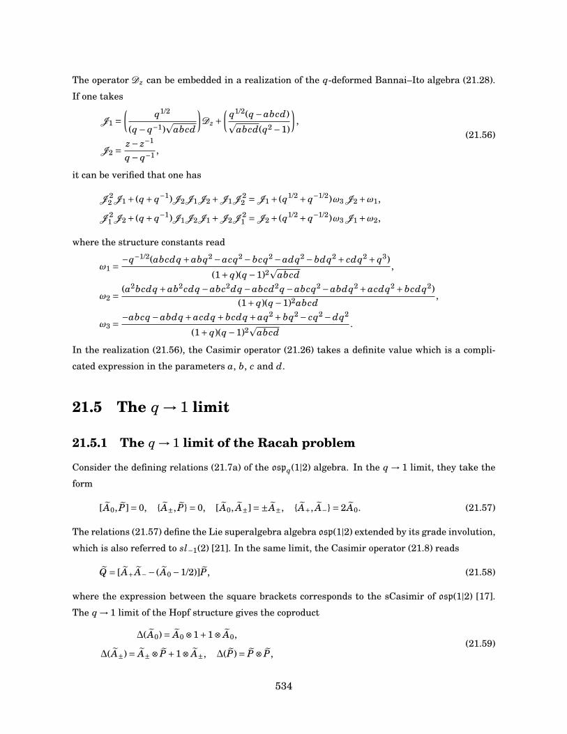
The operator Dz can be embedded in a realization of the q-deformed Bannai–Ito algebra (21.28).
If one takes
J1 =(
q1/2
(q− q−1)p
abcd
)Dz +
(q1/2(q−abcd)p
abcd(q2 −1)
),
J2 = z− z−1
q− q−1 ,
(21.56)
it can be verified that one has
J 22 J1 + (q+ q−1)J2J1J2 +J1J 2
2 =J1 + (q1/2 + q−1/2)ω3 J2 +ω1,
J 21 J2 + (q+ q−1)J1J2J1 +J2J 2
1 =J2 + (q1/2 + q−1/2)ω3 J1 +ω2,
where the structure constants read
ω1 = −q−1/2(abcdq+abq2 −acq2 −bcq2 −adq2 −bdq2 + cdq2 + q3)
(1+ q)(q−1)2p
abcd,
ω2 = (a2bcdq+ab2cdq−abc2dq−abcd2q−abcq2 −abdq2 +acdq2 +bcdq2)(1+ q)(q−1)2abcd
,
ω3 = −abcq−abdq+acdq+bcdq+aq2 +bq2 − cq2 −dq2
(1+ q)(q−1)2p
abcd.
In the realization (21.56), the Casimir operator (21.26) takes a definite value which is a compli-
cated expression in the parameters a, b, c and d.
21.5 The q → 1 limit
21.5.1 The q → 1 limit of the Racah problem
Consider the defining relations (21.7a) of the ospq(1|2) algebra. In the q → 1 limit, they take the
form
[A0, P]= 0, A±, P= 0, [A0, A±]=±A±, A+, A−= 2A0. (21.57)
The relations (21.57) define the Lie superalgebra algebra osp(1|2) extended by its grade involution,
which is also referred to sl−1(2) [21]. In the same limit, the Casimir operator (21.8) reads
Q = [A+ A−− (A0 −1/2)]P, (21.58)
where the expression between the square brackets corresponds to the sCasimir of osp(1|2) [17].
The q → 1 limit of the Hopf structure gives the coproduct
∆(A0)= A0 ⊗1+1⊗ A0,
∆(A±)= A±⊗ P +1⊗ A±, ∆(P)= P ⊗ P,(21.59)
534
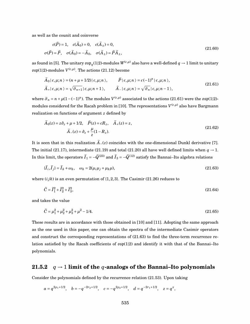
as well as the counit and coinverse
ε(P)= 1, ε(A0)= 0, ε(A±)= 0,
σ(P)= P, σ(A0)=−A0, σ(A±)= P A±,(21.60)
as found in [5]. The unitary ospq(1|2)-modules W (ε,µ) also have a well-defined q → 1 limit to unitary
osp(1|2)-modules V (ε,µ). The actions (21.12) become
A0 | ε,µ;n ⟩ = (n+µ+1/2) | ε,µ;n ⟩, P | ε,µ;n ⟩ = ε (−1)n | ε,µ;n ⟩,A+| ε,µ;n ⟩ =
√σn+1 | ε,µ;n+1 ⟩, A− | ε,µ;n ⟩ =
√σn | ε,µ;n−1 ⟩,
(21.61)
where σn = n+µ(1− (−1)n). The modules V (ε,µ) associated to the actions (21.61) were the osp(1|2)-
modules considered for the Racah problem in [10]. The representations V (ε,µ) also have Bargmann
realization on functions of argument z defined by
A0(z)= z∂z +µ+1/2, P(z)= εRz, A+(z)= z,
A−(z)= ∂z + µ
z(1−Rz).
(21.62)
It is seen that in this realization A−(z) coincides with the one-dimensional Dunkl derivative [7].
The initial (21.17), intermediate (21.19) and total (21.20) all have well defined limits when q → 1.
In this limit, the operators I1 =−Q(23) and I3 =−Q(12) satisfy the Bannai–Ito algebra relations
I i, I j= Ik +ωk, ωk = 2(µiµ j +µkµ), (21.63)
where (i jk) is an even permutation of 1,2,3. The Casimir (21.26) reduces to
C = I21 + I2
2 + I23, (21.64)
and takes the value
C =µ21 +µ2
2 +µ23 +µ2 −1/4. (21.65)
These results are in accordance with those obtained in [10] and [11]. Adopting the same approach
as the one used in this paper, one can obtain the spectra of the intermediate Casimir operators
and construct the corresponding representations of (21.63) to find the three-term recurrence re-
lation satisfied by the Racah coefficients of osp(1|2) and identify it with that of the Bannai–Ito
polynomials.
21.5.2 q → 1 limit of the q-analogs of the Bannai–Ito polynomials
Consider the polynomials defined by the recurrence relation (21.53). Upon taking
a = q2ρ1+1/2, b =−q−2r2+1/2, c =−q2ρ2+1/2, d = q−2r1+1/2, z = qx,
535
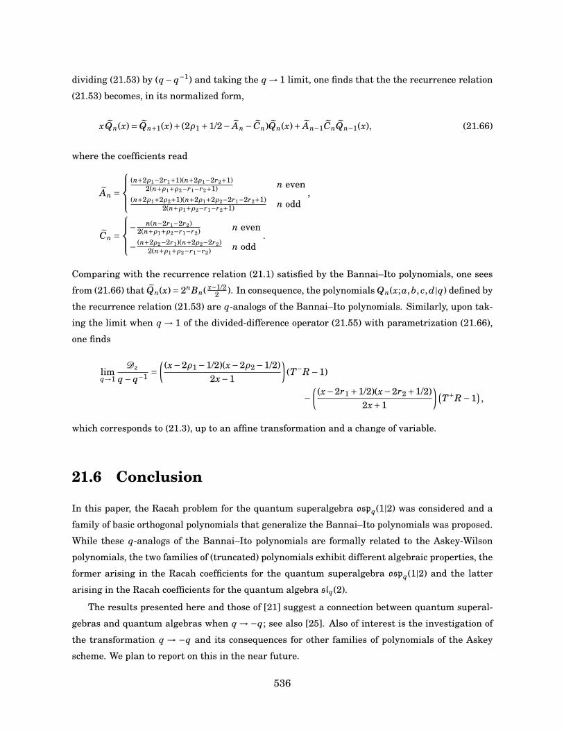
dividing (21.53) by (q− q−1) and taking the q → 1 limit, one finds that the the recurrence relation
(21.53) becomes, in its normalized form,
xQn(x)= Qn+1(x)+ (2ρ1 +1/2− An − Cn)Qn(x)+ An−1CnQn−1(x), (21.66)
where the coefficients read
An =
(n+2ρ1−2r1+1)(n+2ρ1−2r2+1)
2(n+ρ1+ρ2−r1−r2+1) n even(n+2ρ1+2ρ2+1)(n+2ρ1+2ρ2−2r1−2r2+1)
2(n+ρ1+ρ2−r1−r2+1) n odd,
Cn =
− n(n−2r1−2r2)2(n+ρ1+ρ2−r1−r2) n even
− (n+2ρ2−2r1)(n+2ρ2−2r2)2(n+ρ1+ρ2−r1−r2) n odd
.
Comparing with the recurrence relation (21.1) satisfied by the Bannai–Ito polynomials, one sees
from (21.66) that Qn(x)= 2nBn( x−1/22 ). In consequence, the polynomials Qn(x;a,b, c,d|q) defined by
the recurrence relation (21.53) are q-analogs of the Bannai–Ito polynomials. Similarly, upon tak-
ing the limit when q → 1 of the divided-difference operator (21.55) with parametrization (21.66),
one finds
limq→1
Dz
q− q−1 =(
(x−2ρ1 −1/2)(x−2ρ2 −1/2)2x−1
)(T−R−1)
−(
(x−2r1 +1/2)(x−2r2 +1/2)2x+1
)(T+R−1
),
which corresponds to (21.3), up to an affine transformation and a change of variable.
21.6 Conclusion
In this paper, the Racah problem for the quantum superalgebra ospq(1|2) was considered and a
family of basic orthogonal polynomials that generalize the Bannai–Ito polynomials was proposed.
While these q-analogs of the Bannai–Ito polynomials are formally related to the Askey-Wilson
polynomials, the two families of (truncated) polynomials exhibit different algebraic properties, the
former arising in the Racah coefficients for the quantum superalgebra ospq(1|2) and the latter
arising in the Racah coefficients for the quantum algebra slq(2).
The results presented here and those of [21] suggest a connection between quantum superal-
gebras and quantum algebras when q →−q; see also [25]. Also of interest is the investigation of
the transformation q → −q and its consequences for other families of polynomials of the Askey
scheme. We plan to report on this in the near future.
536
References
[1] E. Bannai and T. Ito. Algebraic Combinatorics I. Association Schemes. Benjamin/Cummings
Publishing Company, 1984.
[2] H. De Bie, V. X. Genest, S. Tsujimoto, L. Vinet, and A. Zhedanov. The Bannai-Ito algebra and
some applications. Journal of Physics: Conference Series, 2015.
[3] H. De Bie, V. X. Genest, and L. Vinet. A Dirac-Dunkl equation on S2 and the Bannai-Ito
algebra. ArXiv:1501.03108, 2015.
[4] W. S. Chung, E. G. Kalnins, and W. Miller. Tensor products of q-superalgebras representa-
tions and q-series identities . Journal of Physics A: Mathematical and General, 30(20):7147–
7166, October 1997.
[5] C. Daskaloyannis, K. Kanakoglou, and I. Tsohantjis. Hopf algebraic structure of the para-
bosonic and parafermionic algebras and paraparticle generalization of the Jordan–Schwinger
map. Journal of Mathematical Physics, 41(2):652, February 2000.
[6] J. Van der Jeugt. 3n j-Coefficients and Orthogonal Polynomials of Hypergeometric Type. In
Orthogonal Polynomials and Special Functions, volume 1817 of Lecture Notes in Mathematics
, pages 25–92. 2003.
[7] C. Dunkl. Differential-difference operators associated to reflection groups. Transactions of
the American Mathematical Society, 311(13):167–183, January 1989.
[8] R. Floreanini and L. Vinet. q-analogues of the parabose and parafermi oscillators and
representations of quantum algebras. Journal of Physics A: Mathematical and General,
23(19):L1019, October 1990.
[9] V. X. Genest, L. Vinet, and A. Zhedanov. The Bannai-Ito algebra and a superintegrable sys-
tem with reflections on the two-sphere. Journal of Physics A: Mathematical and Theoretical,
47(20):205202, May 2014.
[10] V. X. Genest, L. Vinet, and A. Zhedanov. The Bannai-Ito polynomials as Racah coefficients
of the sl−1(2) algebra. Proceedings of the American Mathematical Society, 142(5):1545–1560,
May 2014.
[11] V. X. Genest, L. Vinet, and A. Zhedanov. A Laplace-Dunkl equation on S2 and the Bannai–Ito
algebra. Communications in Mathematical Physics (in Press), 2015.
537
[12] Y. A. Granovskii and A. Zhedanov. Nature of the symmetry group of the 6 j symbol. Journal
of Experimental and Theoretical Physics, 94(10):1982–1985, October 1988.
[13] W. Groenevelt. Quantum Analogs of Tensor Product Representations of su(1,1). SIGMA,
7:77, 2011.
[14] R. Koekoek, P. A. Lesky, and R. F. Swarttouw. Hypergeometric orthogonal polynomials and
their q-analogues. Springer, 2010.
[15] T. Koornwinder. The Relationship between Zhedanov’s Algebra AW(3) and the Double Affine
Hecke Algebra in the Rank One Case. SIGMA, 311:63, 2007.
[16] P. P. Kulish and N. Yu Reshetikhin. Universal R-Matrix of the Quantum Superalgebra
osp(1|2). Letters in Mathematical Physics, 18(2):143–149, August 1989.
[17] A. Lesniewski. A remark on the Casimir elements of Lie superalgebras and quantized Lie
superalgebras. Journal of Mathematical Physics, 36(3):1457–1461, March 1995.
[18] P. Minnaert and M. Mozrzymas. Racah coefficients and 6− j symbols for the quantum super-
algebra Uq(osp(1|2)). Journal of Mathematical Physics, 36(2):907, February 1995.
[19] N. Munkunda, E. C. G. Sudarshan, J. K. Sharma, and C. L. Mehta. Representations and
properties of paraBose oscillator operators. I. Energy position and momentum eigenstates.
Journal of Mathematical Physics, 21(9):2386, September 1980.
[20] P. Terwilliger and R. Vidunas. Leonard pairs and the Askey-Wilson relations. Journal of
Algebra and Its Applications, 311(4):411–426, December 2004.
[21] S. Tsujimoto, L. Vinet, and A. Zhedanov. From slq(2) to a parabosonic Hopf algebra. SIGMA,
7:93–105, 2011.
[22] S. Tsujimoto, L. Vinet, and A. Zhedanov. Dunkl shift operators and Bannai–Ito polynomials.
Advances in Mathematics, 229(4):2123–2158, March 2012.
[23] R. G. Underwood. An introduction to Hopf algebras. Springer, 2011.
[24] N. Ja. Vilenkin and A. U. Klimyk. Representation of Lie Groups and Special Functions, vol-
ume 72 of Mathematics and its Applications (Soviet Series). Springer, 1991.
[25] C. K. Zachos. Altering the Symmetry of Wavefunctions in Quantum Algebras and Supersym-
metry. Modern Physics Letters A, 7(18):1595, June 1992.
[26] A. Zhedanov. “Hidden symmetry of Askey-Wilson polynomials. Theoretical and Mathematical
Physics, 89(2):1146–1157, November 1991.
538
Chapitre 22
The equitable presentation of ospq(1|2)
and a q-analog of the Bannai–Itoalgebra
V. X. Genest, L. Vinet et A. Zhedanov (2015). The equitable presentation of ospq(1|2) and a q-
analog of the Bannai–Ito algebra. Soumis à Letters in Mathematical Physics.
Abstract. The equitable presentation of the quantum superalgebra ospq(1|2), in which all gener-
ators appear on an equal footing, is exhibited. It is observed that in their equitable presentations,
the quantum algebras ospq(1|2) and slq(2) are related to one another by the formal transforma-
tion q →−q. A q-analog of the Bannai–Ito algebra is shown to arise as the covariance algebra of
ospq(1|2).
22.1 Introduction
The purpose of this Letter is threefold: to display the equitable, or Z3-symmetric, presentation
of the quantum superalgebra ospq(1|2), to show that the equitable presentations of ospq(1|2) and
slq(2) are related to one another by the formal transformation q →−q, and to demonstrate that
the covariance algebra of ospq(1|2) is a q-analog of the Bannai–Ito algebra.
Our considerations take root in the Racah problem for the su(2) algebra, i.e. the coupling of
three angular momenta. In this problem, the states are usually described in terms of the quan-
tum numbers j i associated to the individual angular momenta ~Ji with i ∈ 1,2,3, the quantum
number j associated to the total angular momentum ~J = ~J1 + ~J2 + ~J3, the quantum number M
associated to the projection of the total angular momentum ~J along one axis, and any one of the
539
quantum numbers j12, j23, j31 associated to the intermediate angular momenta ~Ji j = ~Ji +~J j for
(i j) ∈ (12), (23), (31). These bases are related via Racah coefficients [3]. The main drawback of
such bases is their involved behavior under particle permutations. To circumvent this problem,
Chakrabarti [2], Lévy-Leblond and Lévy-Nahas [20] devised an “equitable” coupling scheme and
showed that there is a “democratic” basis specified by the quantum numbers j1, j2, j3, j and ζ,
where ζ is the eigenvalue of the volume operator ∆= (~J1 ×~J2) ·~J3. The three angular momenta ~Ji
enter symmetrically in this scheme and the states of the democratic basis have definite behaviors
under particle permutations.
The Racah–Wilson algebra is the hidden algebraic structure behind the Racah problems of
su(2) and su(1,1) [11]. The concern for a democratic approach to these Racah problems leads to the
equitable presentation of this algebra [9]. In this presentation, the defining relations of the Racah–
Wilson algebra are Z3-symmetric and all the generators appear on an equal footing, whence the
epithets “equitable” or “democratic”. It was recently shown in [5] that the equitable generators
of the Racah/Wilson algebra can also be realized as quadratic expressions in the equitable sl(2)
generators proposed in [14]. Note that the Racah–Wilson algebra also arises as symmetry algebra
for superintegrable systems [16] and encodes the bispectrality of the Racah/Wilson polynomials
[6].
The Racah problem can also be posited for the quantum algebra slq(2). In this case, it is the
Askey–Wilson algebra [26], also known as the Zhedanov algebra [17], that arises as the hidden
algebraic structure [12]. This algebra encodes the bispectrality of the Askey-Wilson polynomials
and, as shown in [13], arises as the covariance algebra for slq(2). An equitable presentation of
the (universal) Askey-Wilson algebra was offered by Terwilliger in [22] who also showed that it
can be realized by quadratic combinations of the equitable generators of slq(2). The equitable
presentation of slq(2) was itself studied in [15]. A democratic presentation for the quantum group
Uq(g) associated with a symmetrizable Kac-Moody algebra g was also proposed in [21].
In a recent paper [10], the Racah problem for the quantum superalgebra ospq(1|2) was consid-
ered. It was shown that in this case a q-analog of the Bannai–Ito algebra, an algebra proposed
in [24], appears as the “hidden” algebraic structure. The algebra obtained in [10] exhibits a Z3
symmetry and is related to the Askey–Wilson algebra by the formal transformation q →−q.
In this Letter, we display the equitable presentation of the quantum superalgebra ospq(1|2),
determine its relation with the equitable presentation of slq(2) and show that it can be used to
realize the q-analog of the Bannai–Ito algebra defined in [10]. The results that we present here
enrich the understanding of the quintessential quantum superalgebra ospq(1|2) and shed light on
its relationship with other algebraic structures that have appeared recently. The contents of the
Letter are as follows.
In Section 2, the definition of ospq(1|2) is reviewed and its extension by the grade involution is
540
presented. A two-parameter family of ospq(1|2)-modules is defined. The equitable presentation of
ospq(1|2) is introduced and several expressions are given for the Casimir operator. The equitable
presentation of slq(2) is reviewed and compared with the one found for ospq(1|2). In section 3, the
realization of the q-deformed Bannai–Ito algebra in terms of the equitable ospq(1|2) generators is
presented. A short conclusion follows.
22.2 The ospq(1|2) algebra and its equitable presenta-
tion
In this section, we recall the definition of the ospq(1|2) algebra, present its extension by the grade
involution, define a family of irreducible representations and display its equitable presentation.
We review the equitable presentation of slq(2) and compare it with that of ospq(1|2).
22.2.1 Definition of ospq(1|2), the grade involution, and represen-
tations
Let q be a complex number which is not a root of unity and let [n]q denote
[n]q = qn − q−n
q− q−1 .
The quantum superalgebra ospq(1|2) is the Z2-graded unital associative C-algebra generated by
the even element A0 and the odd elements A± satisfying the relations [18]
[A0, A±]=±A±, A+, A−= [2A0]q1/2 ,
where [x, y] = xy− yx and x, y = xy+ yx respectively stand for the commutator and the anticom-
mutator. The sCasimir operator of ospq(1|2) is defined as [19]
S = A+A−− [A0 −1/2]q.
This operator is readily seen to obey the relations
S, A±= 0, [S, A0]= 0.
The abstract Z2-grading of ospq(1|2) can be concretized by adding the grade involution P to the
set of generators and by declaring that the even and odd generators respectively commute and
anticommute with P. The quantum superalgebra ospq(1|2) can thus be presented as the unital
541
associative C-algebra generated by the elements A0, A± and the involution P obeying the relations
[A0, A±]=±A±, A+, A−= [2A0]q1/2 , P, A±= 0, [P, A0]= 0, P2 = 1. (22.1a)
In (22.1a), the parity of the elements no longer needs to be specified. Upon introducing the gener-
ators
K = qA0 , K−1 = q−A0 ,
one can write the relations (22.1a) in the form
K A+K−1 = qA+, K A−K−1 = q−1 A−, KK−1 = 1, P2 = 1,
[K ,P]= 0, [K−1,P]= 0, A±,P= 0, A+, A−= K −K−1
q1/2 − q−1/2 .(22.1b)
It is directly verified that the Casimir operator
Q =(A+A−− [A0 −1/2]q
)P, (22.2)
which is related to the sCasimir operator by Q = SP, commutes with all the generators in (22.1).
The quantum superalgebra ospq(1|2) can be equipped with a Hopf algebraic structure [18]. Intro-
duce the coproduct map ∆ : ospq(1|2)→ ospq(1|2)⊗ospq(1|2) with
∆(A+)= A+⊗KP +1⊗ A+, ∆(A−)= A−⊗P +K−1 ⊗ A−,
∆(K)= K ⊗K , ∆(P)= P ⊗P,(22.3)
the counit map ε : ospq(1|2)→C with
ε(P)= 1, ε(K)= 1, ε(A±)= 0, (22.4)
and the coinverse map σ : ospq(1|2)→ ospq(1|2) with
σ(P)= P, σ(K)= K−1, σ(A+)=−A+K−1P, σ(A−)=−K A−P. (22.5)
It is a straightforward exercise to verify that with the coproduct ∆, the counit ε and the coin-
verse σ defined as in (22.3), (22.4) and (22.5), the algebra (22.1) complies with the well-known
requirements for a Hopf algebra [25].
Remark 9. Let us note that in computing with the coproduct, one should use the standard product
rule (a⊗ b)(c⊗d) = (ac⊗ bd), as opposed to the usual graded product rule used for superalgebras
when the grade involution is not introduced.
542
Let us now bring a two-parameter family of irreducible representations of ospq(1|2). Let ν
be a real parameter and let e = ±1. Moreover, let W (e,ν) be the infinite-dimensional vector space
spanned by the basis vectors f (e,ν)n , where n is a non-negative integer. It is verified that the actions
K f (e,ν)n = qn+ν+1/2 f (e,ν)
n , P f (e,ν)n = e(−1)n f (e,ν)
n ,
A+ f (e,ν)n = f (e,ν)
n+1 , A− f (e,ν)n = ρn f (e,ν)
n−1 ,(22.6)
where
ρn = [n+ν]q − (−1)n[ν]q,
define representations of ospq(1|2) on W (e,ν). For generic values of ν, one has ρn 6= 0 for all n > 1.
As a consequence, these representations are irreducible. On W (e,ν), the Casimir operator (22.2)
acts as a multiple of the identity
Q f (e,ν)n =− e [ν]q f (e,ν)
n ,
as expected from Schur’s lemma. Note that the representations W (e,ν) are associated to the q-
analog of the parabosonic oscillator [4].
Remark 10. It is possible to define finite-dimensional representations of (22.1). Indeed, if one
takes ν = −(N +1)/2, where N is a even integer, one can use the actions (22.6) to define (N +1)-
dimensional irreducible representations of ospq(1|2).
The representations W (e,ν) have a Bargmann realization on functions of the complex argument
z. In this realization, the basis vectors f (e,ν)n ≡ f (e,ν)
n (z) read
f (e,ν)n (z)= zn, n = 0,1,2, . . . ,
and the generators have the expressions
K(z)= qν+1/2 Tq, P(z)= eRz,
A+(z)= z, A−(z)= qν
q− q−1
(Tq −Rz
z
)− q−ν
q− q−1
(T−1
q −Rz
z
),
(22.7)
where Rz g(z)= g(−z) is the reflection operator and where T±q g(z)= g(q±1z) is the q-shift operator.
22.2.2 The equitable presentation of ospq(1|2)
Let X , Y±, Z and ωy be defined as
X = K−1P − (1− q−1)A+K−1P, Y± = K±P, Z = K−1P + (q1/2 + q−1/2)A−P, ωy = P. (22.8)
543
Using the relations (22.1), one readily verifies that these operators satisfy
q1/2XY + q−1/2Y Xq1/2 + q−1/2 = 1,
q1/2Y Z+ q−1/2ZYq1/2 + q−1/2 = 1,
q1/2ZX + q−1/2X Zq1/2 + q−1/2 = 1. (22.9)
In addition to Y Y−1 = 1 and ω2y = 1, one has also the relations
Xωy +ωyX = 2Y−1ωy, Yωy +ωyY = 2Yωy, Zωy +ωyZ = 2Y−1ωy. (22.10)
We refer to the relations (22.9) and (22.10) as the equitable presentation of ospq(1|2) and to the
generators X ,Y±, Z and ωy as the equitable generators. It is observed that in this presentation,
the generators are more or less on an equal footing; some asymmetry occurs in the relations with
the involution ωy given in (22.10). The standard generators of ospq(1|2) can be expressed as follows
in terms of the equitable generators:
A+ = 1− XY1− q−1 , A− = (Z−Y−1)ωy
q1/2 + q−1/2 , K± =Y±ωy, P =ωy. (22.11)
In the equitable presentation, the “normalized” Casimir operator
Υ= (q− q−1)Q, (22.12)
can be written in several different ways. One has
Υ= q1/2X − q−1/2Y + q1/2Z− q1/2XY Z, Υ= q1/2Y − q−1/2Z+ q1/2X − q1/2Y ZX ,
Υ= q1/2Z− q−1/2X + q1/2Y − q1/2ZXY , Υ= q1/2Y − q−1/2Z− q−1/2X + q−1/2ZY X ,
Υ= q1/2Z− q−1/2X − q−1/2Y + q−1/2X ZY , Υ= q1/2X − q−1/2Y − q−1/2Z+ q−1/2Y X Z.
With respect to the presentation (22.8), the coproduct (22.3) has the expression
∆(X )= X ⊗1+Y−1 ⊗ (X −1), ∆(Z)= Z⊗1+Y−1 ⊗ (Z−1),
∆(Y )=Y ⊗Y , ∆(ωy)=ωy ⊗ωy.
On the basis f (e,ν)n , the equitable generators have the actions
X f (e,ν)n = e(−1)nq−(n+ν+1/2)
(f (e,ν)n − (1− q−1) f (e,ν)
n+1
),
Y f (e,ν)n = e(−1)nqn+ν+1/2 f (e,ν)
n ,
Z f (e,ν)n = e(−1)n
(q−(n+ν+1/2) f (e,ν)
n + (q1/2 + q−1/2)ρn f (e,ν)n−1
).
(22.13)
22.2.3 The equitable presentation of slq(2)
Let us now establish the relation between the equitable presentations of ospq(1|2) and slq(2). The
quantum algebra slq(2) is defined as the unital C-algebra with generators κ±, J+, J− and relations
κκ−1 = κ−1κ= 1, κJ+κ−1 = qJ+, κJ−κ−1 = q−1J−, [J+, J−]= κ−κ−1
q1/2 − q−1/2 . (22.14)
544
The equitable generators x, y± and z of slq(2) are given by [15]
x = κ−1 − (q1/2 − q−1/2)J+κ−1, y± = κ±, z = κ−1 + (1− q−1)J−, (22.15)
and satisfy the relations
q1/2xy− q−1/2 yxq1/2 − q−1/2 = 1,
q1/2 yz− q−1/2zyq1/2 − q−1/2 = 1,
q1/2zx− q−1/2xzq1/2 − q−1/2 = 1. (22.16)
It is directly seen that the equitable presentation of slq(2) given in (22.16) and the equitable pre-
sentation of ospq(1|2) given in (22.9) are related to one another by the formal transformation
q → −q. This formal relation can also be observed using the standard presentations (22.1) and
(22.14). Indeed, upon defining the generators
κ= KP, κ−1 = K−1P, J+ = 1i
(1− q−1
q1/2 + q−1/2
)A+, J− =
(q1/2 + q−1/2
1+ q−1
)A−P,
one finds that they satisfy the relations
κκ−1 = κ−1κ= 1, κJ+κ−1 =−qJ+, κJ−κ−1 =−q−1 J−, [J+, J−]= κ− κ−1
i(q1/2 + q−1/2),
which indeed corresponds to (22.14) with q →−q.
Remark 11. Note that if one artificially introduces an involution ωy with J±,ωy= 0 and [κ,ωy]=0, relations of the form (22.10) also appear in the equitable presentation of slq(2).
22.3 A q-generalization of the Bannai–Ito algebra and
the covariance algebra of ospq(1|2)
In this section, the definitions of the Bannai–Ito algebra and that of its q-extension are reviewed.
It is shown that the Z3-symmetric q-deformed Bannai–Ito algebra can be realized in terms of the
equitable ospq(1|2) generators.
22.3.1 The Bannai–Ito algebra and its q-extension
The Bannai–Ito algebra first arose in [24] as the algebraic structure encoding the bispectral prop-
erties of the Bannai–Ito polynomials. It also appears as the hidden algebra behind the Racah
problem for the Lie superalgebra osp(1|2) [8] and as a symmetry algebra for superintegrable sys-
tems [1, 7]. The Bannai–Ito algebra is unital associative algebra over C with generators K1, K2,
K3 and relations
K1,K2= K3 +α3, K2,K3= K1 +α1, K3,K1= K2 +α2, (22.17)
545

where αi, i = 1,2,3, are structure constants. This algebra admits the Casimir operator
L = K21 +K2
2 +K23 , (22.18)
which commutes with every generator K i, i = 1,2,3. In [10], a q-deformation of the algebra (22.17)
was identified in the study of the Racah problem for ospq(1|2). This q-extension has generators I1,
I2, I3 and relations
I1, I2q = I3 + ι3, I2, I3q = I1 + ι1, I3, I1q = I2 + ι2, (22.19)
where ι1, ι2, ι3 are structure constants and where
A,Bq = q1/2 AB+ q−1/2BA, (22.20)
is the q-anticommutator. The algebra (22.19) is formally related to the Zhedanov algebra by the
transformation q →−q [10]. It has for Casimir operator
Λ= (q−1/2 − q3/2)I1I2I3 + qI21 + q−1I2
2 + qI23 − (1− q) ι1 I1 − (1− q−1) ι2 I2 − (1− q) ι3 I3, (22.21)
which commutes with all generators I i, i = 1,2,3. It is easily seen that in the limit q → 1, the
relations (22.19) and the expression (22.21) tend to the relations (22.17) and to the relation (22.18).
22.3.2 Covariance algebra of ospq(1|2)
Let a±, b±, c± be complex parameters and consider the operators A, B, C defined as follows:
A = aX −a−1Y + bc−1 (XY −Y X )q1/2 + q−1/2 , B = bY −b−1Z+ ca−1 (Y Z−ZY )
q1/2 + q−1/2 ,
C = cZ− c−1X + ab−1 (ZX − X Z)q1/2 + q−1/2 ,
(22.22)
where X , Y and Z are the equitable generators of ospq(1|2) defined in (22.8). A direct calculation
shows that the elements A, B and C satisfy the relations
q1/2 AB+ q−1/2BAq− q−1 = C+ (a−a−1)(b−b−1)− (c− c−1)Υ
q1/2 − q−1/2 ,
q1/2BC+ q−1/2CBq− q−1 = A+ (b−b−1)(c− c−1)− (a−a−1)Υ
q1/2 − q−1/2 ,
q1/2CA+ q−1/2 ACq− q−1 = B+ (c− c−1)(a−a−1)− (b−b−1)Υ
q1/2 − q−1/2 ,
(22.23)
where Υ is the normalized Casimir operator (22.12) of ospq(1|2). The algebra (22.23) is easily seen
to be equivalent to the q-deformed Bannai–Ito algebra (22.19). Indeed, upon taking
M1 = Aq− q−1 , M2 = B
q− q−1 , M3 = Cq− q−1 , (22.24)
546

one finds that the elements M1, M2, M3 satisfy the defining relations (22.19) of the q-deformed
Bannai–Ito algebra
M1, M2q = M3 +m3, M2, M3q = M1 +m1, M3, M1q = M2 +m2, (22.25)
where the structure constants m1, m2 and m3 read
m1 = (q1/2 + q−1/2)(
(b−b−1)(c− c−1)− (a−a−1)Υ(q− q−1)2
),
m2 = (q1/2 + q−1/2)(
(c− c−1)(a−a−1)− (b−b−1)Υ(q− q−1)2
),
m3 = (q1/2 + q−1/2)(
(a−a−1)(b−b−1)− (c− c−1)Υ(q− q−1)2
).
(22.26)
The presentation (22.25), (22.26) is clearly invariant with respect to the simultaneous cyclic per-
mutation of the generators (M1, M2, M3) and arbitrary parameters (a,b, c); it is thus Z3-symmetric.
In this realization, the Casimir operator (22.21) of the q-deformed Bannai–Ito algebra takes the
definite value
Λ=(
(a−a−1)(b−b−1)(c− c−1)Υ(q− q−1)2
)
+(
a−a−1
q− q−1
)2
+(
b−b−1
q− q−1
)2
+(
c− c−1
q− q−1
)2
+(
Υ
q− q−1
)2− q
(1+ q)2 . (22.27)
In view of the above results, one can conclude that the q-deformed Bannai–Ito algebra serves as
the covariance algebra for ospq(1|2).
Remark 12. Let us note that if one takes a = qα, b = qβ, c = qγ and Υ=−(qδ− q−δ), the structure
constants (22.26) and the Casimir value (22.27) are identical to the ones arising in the Racah
problem for ospq(1|2) [10].
22.4 Conclusion
In this Letter, the equitable presentation of the quantum superalgebra ospq(1|2) was displayed. It
was observed that ospq(1|2) and slq(2) are related by the formal transformation q →−q and it was
established that the q-deformed Bannai–Ito algebra arises as the covariance algebra of ospq(1|2).
Under the appropriate reparametrization, the q-deformed Bannai–Ito algebra (22.25) with
structure constants (22.26) tends to the Bannai–Ito algebra in the q → 1 limit. Similarly in the
limit q → 1 the quantum superalgebra ospq(1|2) defined in (22.1) tends to the Lie superalgebra
osp(1|2) extended by its grade involution, also known as sl−1(2) [23]. However one observes that
547
the operators of the realization (22.8), (22.22), (22.24) do not have a well-defined q → 1 limit. Con-
sequently, one cannot conclude from the above results that the Bannai–Ito algebra is a covariance
algebra of osp(1|2). The interesting problem of realizing the Bannai–Ito algebra in terms of the
Lie superalgebra osp(1|2) thus remains.
References
[1] H. De Bie, V. X. Genest, and L. Vinet. A Dirac-Dunkl equation on S2 and the Bannai-Ito
algebra. ArXiv:1501.03108, 2015.
[2] A. Chakrabarti. On the coupling of 3 angular momenta. Annales de l’Institut Henri Poincaré,
Section A, 1(3):301–327, 1964.
[3] A. R. Edmonds. Angular Momentum in Quantum Mechanics. Investigations in Physics.
Princeton University Press, 1996.
[4] R. Floreanini and L. Vinet. q-analogues of the parabose and parafermi oscillators and
representations of quantum algebras. Journal of Physics A: Mathematical and General,
23(19):L1019, October 1990.
[5] S. Gao, Y. Wang, and B. Hou. The classification of Leonard triples of Racah type. Linear
Algebra and its Applications, 439(7):1834–1861, October 2013.
[6] V. X. Genest, L. Vinet, and A. Zhedanov. Superintegrability in Two Dimensions and the
Racah–Wilson Algebra. Letters in Mathematical Physics, 104(8):931–952, August 2014.
[7] V. X. Genest, L. Vinet, and A. Zhedanov. The Bannai-Ito algebra and a superintegrable sys-
tem with reflections on the two-sphere. Journal of Physics A: Mathematical and Theoretical,
47(20):205202, May 2014.
[8] V. X. Genest, L. Vinet, and A. Zhedanov. The Bannai-Ito polynomials as Racah coefficients
of the sl−1(2) algebra. Proceedings of the American Mathematical Society, 142(5):1545–1560,
May 2014.
[9] V. X. Genest, L. Vinet, and A. Zhedanov. The equitable Racah algebra from three su(1,1)
algebras. Journal of Physics A: Mathematical and Theoretical, 47(2):025203, January 2014.
[10] V. X. Genest, L. Vinet, and A. Zhedanov. The quantum superalgebra ospq(1|2) and a q-
generalization of the Bannai–Ito polynomials. ArXiv:1501.05602, 2015.
548
[11] Y. A. Granovskii and A. Zhedanov. Nature of the symmetry group of the 6 j symbol. Journal
of Experimental and Theoretical Physics, 94(10):1982–1985, October 1988.
[12] Y. A. Granovskii and A. Zhedanov. Hidden symmetry of the Racah and Clebsch-Gordan prob-
lems for the quantum algebra slq(2). Journal of Group Theory in Physics, 1:161–171, 1993.
[13] Y. A. Granovskii and A. Zhedanov. Linear covariance algebra for SLq(2) . Journal of Physics
A: Mathematical and General, 26(7):L357–L359, April 1993.
[14] B. Hartwig and P. Terwilliger. The Tetrahedron algebra, the Onsager algebra, and the sl2
loop algebra. Journal of Algebra, 308(2):840–863, February 2007.
[15] T. Ito, P. Terwilliger, and C. Weng. The quantum algebra Uq(sl2) and its equitable presenta-
tion. Journal of Algebra, 298(1-2):284–301, April 2006.
[16] E. G. Kalnins, W. Miller, and S. Post. Wilson polynomials and the generic superintegrable
system on the 2-sphere. Journal of Physics A: Mathematical and Theoretical, 40(38):11525,
September 2007.
[17] T. Koornwinder. The Relationship between Zhedanov’s Algebra AW(3) and the Double Affine
Hecke Algebra in the Rank One Case. SIGMA, 311:63, 2007.
[18] P. P. Kulish and N. Yu Reshetikhin. Universal R-Matrix of the Quantum Superalgebra
osp(1|2). Letters in Mathematical Physics, 18(2):143–149, August 1989.
[19] A. Lesniewski. A remark on the Casimir elements of Lie superalgebras and quantized Lie
superalgebras. Journal of Mathematical Physics, 36(3):1457–1461, March 1995.
[20] J. M. Lévy-Leblond and M. Lévy-Nahas. Symmetrical Coupling of Three Angular Momenta.
Journal of Mathematical Physics, 6(9):1372, September 1965.
[21] P. Terwilliger. The equitable presentation for the quantum group Uq(g) associated with a
symmetrizable Kac–Moody algebra g. Journal of Algebra, 298(1-2):302–319, April 2006.
[22] P. Terwilliger. The Universal Askey–Wilson Algebra and the Equitable Presentation of
Uq(sl2). SIGMA, 7:99, 2011.
[23] S. Tsujimoto, L. Vinet, and A. Zhedanov. From slq(2) to a parabosonic Hopf algebra. SIGMA,
7:93–105, 2011.
[24] S. Tsujimoto, L. Vinet, and A. Zhedanov. Dunkl shift operators and Bannai–Ito polynomials.
Advances in Mathematics, 229(4):2123–2158, March 2012.
549
[25] R. G. Underwood. An introduction to Hopf algebras. Springer, 2011.
[26] A. Zhedanov. “Hidden” symmetry of Askey-Wilson polynomials. Theoretical and Mathemati-
cal Physics, 89(2):1146–1157, November 1991.
550
Partie IV
Problème de Racah et systèmessuperintégrables
551

Introduction
Le problème de Racah est un problème classique en physique et en théorie de la représentation.
Afin d’être concrets, considérons le cas de su(2) [64]. Les représentations irréductibles Vj de su(2)
décrivent les particules élémentaires de spin j ∈ 0,1/2,1, . . .. Le produit tensoriel V =Vj1⊗Vj2⊗Vj3
correspond au système physique formé de trois particules indépendantes de spins j1, j2 et j3. Du
point de vue de la théorie du moment angulaire, il existe deux bases naturelles pour décrire les
états de ce système. Dans la première base, les états sont étiquetés par les nombres quantiques
j12, j et m, qui correspondent respectivement au moment angulaire du sous-système formé des
particules 1 et 2, au moment angulaire total du système et à la valeur de sa projection sur un axe
donné. Dans le seconde base, les états sont étiquetés par des nombres quantiques j23, j et m, qui
correspondent respectivement au moment angulaire du sous-système formé des particules 2 et 3,
au moment angulaire du système complet et à la valeur de sa projection sur un axe donné. Le
problème de Racah pour l’algèbre su(2) consiste à déterminer les coefficients de transition entre
ces deux bases.
De manière plus générale, le problème de Racah se présente lorsqu’on considère le produit
tensoriel de trois représentations irréductibles d’une algèbre A donnée, dont la nature dépend du
système physique que l’on souhaite considérer.
Dans cette partie de la thèse, on démontre l’équivalence entre le problème de Racah pour
l’algèbre su(1,1) et le système superintégrable générique sur la 2-sphère. La découverte inatten-
due de cette équivalence permet entre autres d’expliquer la nature des symétries de ce système
superintégrable important. En outre, on montre l’équivalence entre le problème de Racah pour
la superalgèbre de Lie osp(1|2) et le système superintégrable générique avec réflexions sur la 2-
sphère.
553

554
Chapitre 23
Superintegrability in two dimensionsand the Racah-Wilson algebra
V. X. Genest, L. Vinet et A. Zhedanov (2014). Superintegrability in two dimensions and the Racah-
Wilson algebra. Letters in Mathematical Physics 104 931–952.
Abstract. The analysis of the most general second-order superintegrable system in two dimen-
sions: the generic 3-parameter model on the 2-sphere, is cast in the framework of the Racah prob-
lem for the su(1,1) algebra. The Hamiltonian of the 3-parameter system and the generators of its
quadratic symmetry algebra are seen to correspond to the total and intermediate Casimir opera-
tors of the combination of three su(1,1) algebras, respectively. The construction makes explicit the
isomorphism between the Racah-Wilson algebra, which is the fundamental algebraic structure be-
hind the Racah problem for su(1,1), and the invariance algebra of the generic 3-parameter system.
It also provides an explanation for the occurrence of the Racah polynomials as overlap coefficients
in this context. The irreducible representations of the Racah-Wilson algebra are reviewed as well
as their connection with the Askey scheme of classical orthogonal polynomials.
23.1 Introduction
The purpose of this paper is to stress the algebraic equivalence between the analysis of the generic
quantum 3-parameter superintegrable system on the 2-sphere and the Racah problem of su(1,1).
The equivalence will be made explicit by the direct identification of the natural operators of the
Racah problem, i.e. the intermediate Casimir operators for the combination of three su(1,1) alge-
bras, with the symmetry operators that span the invariance algebra of the system. From this iden-
tification will follow the explicit isomorphism between the symmetry algebra of the 3-parameter
555
model and the Racah-Wilson algebra, which is the algebra behind the Racah problem for su(1,1).
Since the Racah-Wilson algebra is also the algebraic structure that encodes the properties of the
Racah and Wilson polynomials, the isomorphism will also provide an elegant explanation for the
occurrence of these families of polynomials as overlap coefficients in the 3-parameter system on
the 2-sphere.
23.1.1 The Racah-Wilson algebra
The Racah-Wilson algebra is the infinite-dimensional associative algebra generated by the alge-
braically independent elements K1, K2 that satisfy, together with their commutator K3 ≡ [K1,K2],
the following commutation relations:
[K2,K3]= a2K22 +a1K1,K2+ c1K1 +dK2 + e1,
[K3,K1]= a1K21 +a2K1,K2+ c2K2 +dK1 + e2,
(23.1)
where the structure constants are assumed to be real (it will be seen that the number of structure
constants can be reduced from seven to three by affine transformations of the generators). The
algebra (23.1) first appeared in the coupling problem of three angular momenta, i.e. the Racah
problem for su(2) [8]. It was first observed in [8] that the intermediate Casimir operators in the
combination of three angular momenta realize the algebra (23.1) and this observation was ex-
ploited to derive the symmetry group of the 6 j-symbol (Racah coefficients). In the same paper, a
special case of (23.1) corresponding to a1 = 0 was also seen to occur in the Clebsch-Gordan problem
of su(2) and the algebraic relations were used to find the symmetries of the 3 j coefficients. The rep-
resentations of the algebra (23.1) were presented to some extent in [9] and the link between these
representations and the Askey scheme of classical orthogonal polynomials was established. More
specifically, it was shown that for certain finite(infinite)-dimensional irreducible representations of
(23.1), the Racah (Wilson) polynomials occur as overlap coefficients between the eigenbases of K1
and K2. Furthermore, a suitable generalization of (23.1) whose representations encompass the full
Askey scheme of basic or q-orthogonal polynomials was also proposed; this generalization is now
referred to as the Askey-Wilson algebra [32]. A number of papers followed in which special cases of
the algebra (23.1) were seen to occur as symmetry algebras of classical and quantum second-order
superintegrable systems in two dimensions [4, 10, 11], some of them based on the combination
of two su(1,1) algebras [33], i.e. the Clebsch-Gordan problem for su(1,1). Quite interestingly, the
full Racah algebra was not encountered then. It was only later, with the complete classification
of second-order superintegrable systems, that a significant step in this direction was made in the
study of the generic 3-parameter system on the 2-sphere [20]. Before discussing this particular
model and the results of [20], let us first recall a few points about quantum superintegrability.
556

23.1.2 Superintegrability
A quantum system described by a Hamiltonian H with d degrees of freedom is maximally super-
integrable if it admits 2d−1 algebraically independent symmetry operators Si satisfying
[H,Si]= 0, 16 i 6 2d−1,
where one the symmetries is the Hamiltonian itself, e.g. S1 ≡ H. For such a system, it is impossible
for all the Si to commute with one another and hence the symmetries generate a non-Abelian
invariance algebra for H. In practice, the associated Schrödinger equation
HΨ= Eψ,
can be exactly solved both analytically and algebraically. A superintegrable system is said to be
order ` if ` is the maximum order of the symmetries (excluding H) in the momentum variables.
First order superintegrable systems (` = 1) have geometrical symmetries and their invariance
algebras are Lie algebras [26]. Second order superintegrable systems (`= 2) typically admit sep-
aration of variables in more than one coordinate system and have quadratic symmetry algebras
[12, 13, 25, 27]. In two dimensions, all first and second order superintegrable systems are known
and have been classified [2, 3, 18, 19, 31]. The study of superintegrable systems is important in its
own right in view of their numerous applications. They also constitute a bedrock for the analysis
of symmetries.
23.1.3 The generic 3-parameter system on the 2-sphere
In two dimensions, one of the most important second-order superintegrable systems is the generic
3-parameter model on the 2-sphere [22]. This model is described by the Hamiltonian
H = J21 + J2
2 + J23 + k2
1 − 14
x21
+ k22 − 1
4
x22
+ k23 − 1
4
x23
, (23.2)
with the constraint x21 + x2
2 + x23 = 1. The operators Ji, i = 1,2,3, stand for the standard angular
momentum generators
J1 =−i(x2∂x3 − x3∂x2), J2 =−i(x3∂x1 − x1∂x3), J3 =−i(x1∂x2 − x2∂x1), (23.3)
which satisfy the familiar so(3) commutation relations
[Ji, J j]= i3∑
k=1εi jk Jk, (23.4)
where εi jk is the totally antisymmetric tensor and ∂xi denotes differentiation with respect to the
variable xi. It is known (see [22] and references therein) that all second-order superintegrable
557
models in two dimensions are limiting cases of (23.2); hence the generic 3-parameter model on
the 2-sphere described by the Hamiltonian (23.2) can be considered as the most general system of
such type. The symmetries of H and the quadratic invariance algebra they span can be found in
[17, 19]. Upon taking
L1 = J21 + a2x2
3
x22
+ a3x22
x23
, L2 = J22 + a3x2
1
x23
+ a1x23
x21
, L3 = J23 + a1x2
2
x21
+ a2x21
x22
, (23.5)
where a1 = k21 −1/4, a2 = k2
2 −1/4 and a3 = k23 −1/4, it is directly checked that [H ,L i] = 0, i.e. that
the operators L i are constants of motion. Furthermore, upon defining R = [L1,L2], the following
commutation relations hold:
[L i,R]= 4L i,L j−4L i,Lk− (8−16a j)L j + (8−16ak)Lk +8(a j −ak), (23.6)
where x, y = xy+ yx stands for the anticommutator. The four symmetry operators L1, L2, L3, R
and the Hamiltonian H are not algebraically independent from one another. Indeed, one has
H = L1 +L2 +L3 +a1 +a2 +a3, (23.7)
which relates the sum of the three symmetries (23.5) to the Hamiltonian. Moreover, the square of
the symmetry operator R can be shown to satisfy [19]
R2 =− 83
L1,L2,L3−3∑
i=1
(12−16ai)L2
i +13
(16−176ai)L i + 323
ai
+ 52
3(L1,L2+ L2,L3+ L1,L3)+48(a1a2 +a2a3 +a3a1)−64a1a2a3,
(23.8)
where x1, x2, x3 is the symmetrized sum of six terms of the form xix jxk. In view of the rela-
tions (23.7) and (23.8), it is clear that the system described by the Hamiltonian (23.2) possesses
three algebraically independent symmetries: H , L1, L2, and is hence maximally superintegrable.
Moreover, since L1, L2 are second order differential operators, the generic 3-parameter system
of the sphere is superintegrable of order ` = 2. The solutions of the Schrödinger equation associ-
ated to H have been obtained in [17] by separation of variables in various coordinate systems. In
spherical coordinates, these solutions are given in terms of the classical Jacobi polynomials.
23.1.4 The 3-parameter system and Racah polynomials
In a remarkable paper [20], the finite(infinite)-dimensional irreducible representations of the sym-
metry algebra (23.6), (23.8) have been related to the Racah (Wilson) polynomials. More specifically,
it was shown that this symmetry algebra can be realized in terms of difference operators of which
the Racah (Wilson) polynomials are eigenfunctions. Given the complexity of the algebraic relations
(23.6), (23.8), the result constitutes a tour de force. It also implies that the Racah polynomials act
558
as overlap coefficients between the eigenbases of L1 and L2 in a given energy eigenspace of the
Hamiltonian (23.2). Moreover it allows, through contractions [22], to tie the entire Askey scheme
of classical orthogonal polynomials to physical systems.
The occurrence of the Racah (Wilson) polynomials in the representations of the symmetry al-
gebra of the 3-parameter model strongly suggests that the symmetry algebra (23.6), (23.8) can
be explicitly written in the form (23.1). More importantly, it indicates the existence of a connec-
tion between the 3-parameter system and the Racah problem of either su(1,1) or su(2), for which
the Racah-Wilson algebra is the underlying algebraic structure. As suggested by the work of
Kuznetsov [24] and by [33], the connection will be made through the su(1,1) algebra. It will be
shown explicitly that the analysis of the generic 3-parameter system on the 2-sphere is equivalent
to the Racah problem for su(1,1). Using a realization of su(1,1) in terms of differential operators,
the 3-parameter Hamiltonian (23.2) will be seen to correspond to the total Casimir operator of
the combination of three su(1,1) algebras and the symmetries L1, L2, L3 will be identified with
the intermediate Casimir operators. From this identification will follow the explicit isomorphism
between the invariance algebra (23.6), (23.8) and the Racah-Wilson algebra which, as we recall, is
the fundamental algebraic structure for both the Racah problem for su(1,1) and the Askey-Scheme
of classical orthogonal polynomials.
23.1.5 Outline
The outline of the paper is as follows. In section 2, the connection between the finite-dimensional
irreducible representations of Racah-Wilson algebra and the Racah polynomials is established.
This connection is obtained in two equivalent ways. First, the finite-dimensional irreducible rep-
resentations of the Racah-Wilson algebra are developed in a model-independent fashion and are
then related to the Racah polynomials. Second, it is shown that the difference operators corre-
sponding to the difference equation and recurrence relation of the Racah polynomials realize the
Racah-Wilson algebra (23.1). The reader who wishes to focus on the connection between the Racah
problem and superintegrability could proceeed directly to subsection 2.4. In section 3, the analy-
sis of the Racah problem for su(1,1) by means of the Racah algebra is revisited. In section 4, the
equivalence between the Racah problem for su(1,1) and the generic 3-parameter superintegrable
system is established using a differential realization of su(1,1). The isomorphism between the
invariance algebra of the model and the quadratic Racah algebra is written down explicitly. Some
perspectives on future investigations are offered in the conclusion.
559
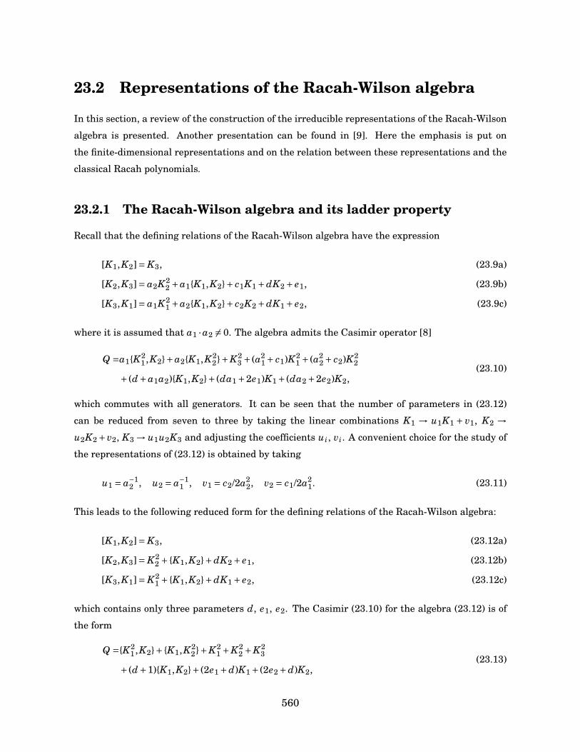
23.2 Representations of the Racah-Wilson algebra
In this section, a review of the construction of the irreducible representations of the Racah-Wilson
algebra is presented. Another presentation can be found in [9]. Here the emphasis is put on
the finite-dimensional representations and on the relation between these representations and the
classical Racah polynomials.
23.2.1 The Racah-Wilson algebra and its ladder property
Recall that the defining relations of the Racah-Wilson algebra have the expression
[K1,K2]= K3, (23.9a)
[K2,K3]= a2K22 +a1K1,K2+ c1K1 +dK2 + e1, (23.9b)
[K3,K1]= a1K21 +a2K1,K2+ c2K2 +dK1 + e2, (23.9c)
where it is assumed that a1 ·a2 6= 0. The algebra admits the Casimir operator [8]
Q =a1K21 ,K2+a2K1,K2
2+K23 + (a2
1 + c1)K21 + (a2
2 + c2)K22
+ (d+a1a2)K1,K2+ (da1 +2e1)K1 + (da2 +2e2)K2,(23.10)
which commutes with all generators. It can be seen that the number of parameters in (23.12)
can be reduced from seven to three by taking the linear combinations K1 → u1K1 + v1, K2 →u2K2 +v2, K3 → u1u2K3 and adjusting the coefficients ui, vi. A convenient choice for the study of
the representations of (23.12) is obtained by taking
u1 = a−12 , u2 = a−1
1 , v1 = c2/2a22, v2 = c1/2a2
1. (23.11)
This leads to the following reduced form for the defining relations of the Racah-Wilson algebra:
[K1,K2]= K3, (23.12a)
[K2,K3]= K22 + K1,K2+dK2 + e1, (23.12b)
[K3,K1]= K21 + K1,K2+dK1 + e2, (23.12c)
which contains only three parameters d, e1, e2. The Casimir (23.10) for the algebra (23.12) is of
the form
Q =K21 ,K2+ K1,K2
2+K21 +K2
2 +K23
+ (d+1)K1,K2+ (2e1 +d)K1 + (2e2 +d)K2,(23.13)
560
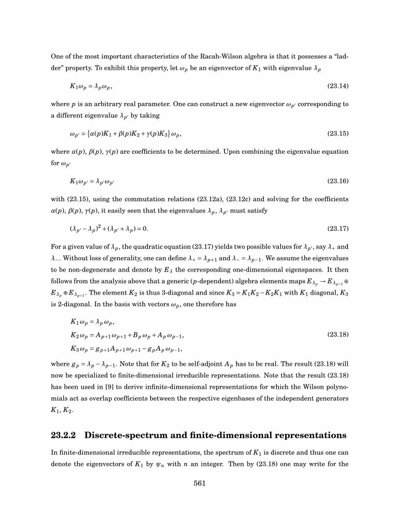
One of the most important characteristics of the Racah-Wilson algebra is that it possesses a “lad-
der” property. To exhibit this property, let ωp be an eigenvector of K1 with eigenvalue λp
K1ωp =λpωp, (23.14)
where p is an arbitrary real parameter. One can construct a new eigenvector ωp′ corresponding to
a different eigenvalue λp′ by taking
ωp′ = α(p)K1 +β(p)K2 +γ(p)K3
ωp, (23.15)
where α(p), β(p), γ(p) are coefficients to be determined. Upon combining the eigenvalue equation
for ωp′
K1ωp′ =λp′ωp′ (23.16)
with (23.15), using the commutation relations (23.12a), (23.12c) and solving for the coefficients
α(p), β(p), γ(p), it easily seen that the eigenvalues λp, λp′ must satisfy
(λp′ −λp)2 + (λp′ +λp)= 0. (23.17)
For a given value of λp, the quadratic equation (23.17) yields two possible values for λp′ , say λ+ and
λ−. Without loss of generality, one can define λ+ =λp+1 and λ− =λp−1. We assume the eigenvalues
to be non-degenerate and denote by Eλ the corresponding one-dimensional eigenspaces. It then
follows from the analysis above that a generic (p-dependent) algebra elements maps Eλp → Eλp−1⊕Eλp ⊕Eλp+1 . The element K2 is thus 3-diagonal and since K3 = K1K2−K2K1 with K1 diagonal, K3
is 2-diagonal. In the basis with vectors ωp, one therefore has
K1ωp =λpωp,
K2ωp = Ap+1ωp+1 +Bpωp + Apωp−1,
K3ωp = gp+1 Ap+1ωp+1 − gp Apωp−1,
(23.18)
where gp =λp −λp−1. Note that for K2 to be self-adjoint Ap has to be real. The result (23.18) will
now be specialized to finite-dimensional irreducible representations. Note that the result (23.18)
has been used in [9] to derive infinite-dimensional representations for which the Wilson polyno-
mials act as overlap coefficients between the respective eigenbases of the independent generators
K1, K2.
23.2.2 Discrete-spectrum and finite-dimensional representations
In finite-dimensional irreducible representations, the spectrum of K1 is discrete and thus one can
denote the eigenvectors of K1 by ψn with n an integer. Then by (23.18) one may write for the
561
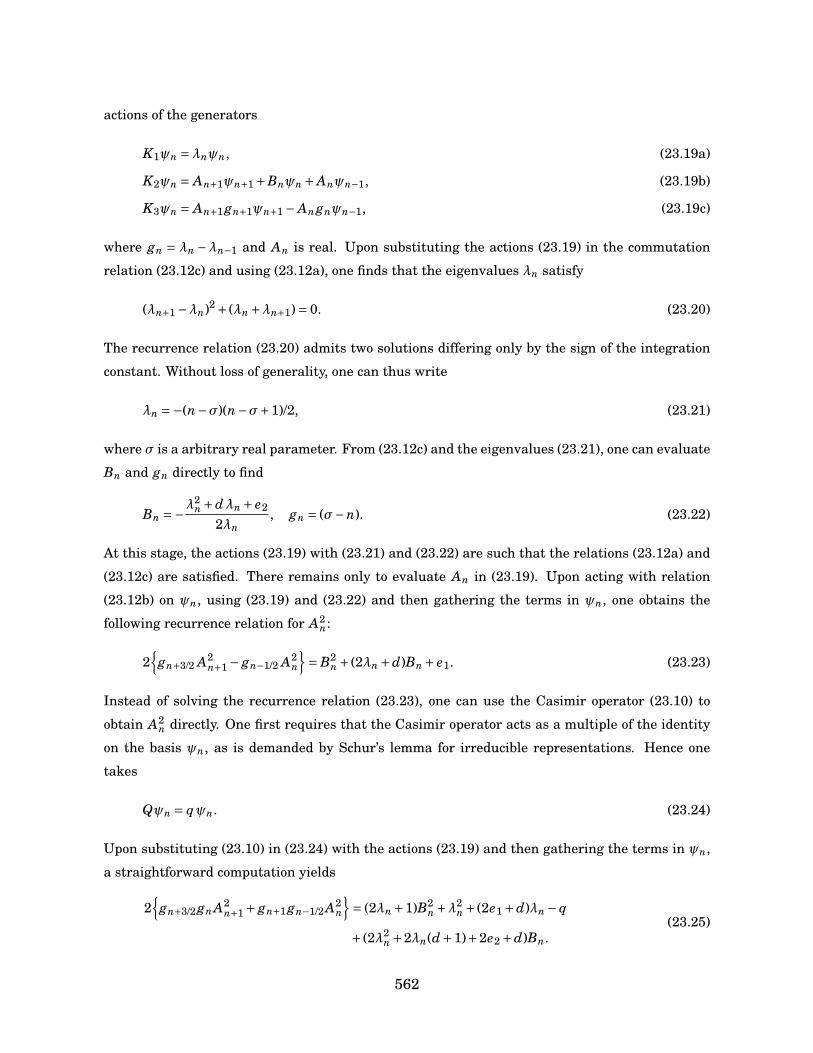
actions of the generators
K1ψn =λnψn, (23.19a)
K2ψn = An+1ψn+1 +Bnψn + Anψn−1, (23.19b)
K3ψn = An+1 gn+1ψn+1 − An gnψn−1, (23.19c)
where gn = λn −λn−1 and An is real. Upon substituting the actions (23.19) in the commutation
relation (23.12c) and using (23.12a), one finds that the eigenvalues λn satisfy
(λn+1 −λn)2 + (λn +λn+1)= 0. (23.20)
The recurrence relation (23.20) admits two solutions differing only by the sign of the integration
constant. Without loss of generality, one can thus write
λn =−(n−σ)(n−σ+1)/2, (23.21)
where σ is a arbitrary real parameter. From (23.12c) and the eigenvalues (23.21), one can evaluate
Bn and gn directly to find
Bn =−λ2n +dλn + e2
2λn, gn = (σ−n). (23.22)
At this stage, the actions (23.19) with (23.21) and (23.22) are such that the relations (23.12a) and
(23.12c) are satisfied. There remains only to evaluate An in (23.19). Upon acting with relation
(23.12b) on ψn, using (23.19) and (23.22) and then gathering the terms in ψn, one obtains the
following recurrence relation for A2n:
2
gn+3/2 A2n+1 − gn−1/2 A2
n
= B2
n + (2λn +d)Bn + e1. (23.23)
Instead of solving the recurrence relation (23.23), one can use the Casimir operator (23.10) to
obtain A2n directly. One first requires that the Casimir operator acts as a multiple of the identity
on the basis ψn, as is demanded by Schur’s lemma for irreducible representations. Hence one
takes
Qψn = qψn. (23.24)
Upon substituting (23.10) in (23.24) with the actions (23.19) and then gathering the terms in ψn,
a straightforward computation yields
2
gn+3/2 gn A2n+1 + gn+1 gn−1/2 A2
n
= (2λn +1)B2
n +λ2n + (2e1 +d)λn − q
+ (2λ2n +2λn(d+1)+2e2 +d)Bn.
(23.25)
562
Combining (23.23) and (23.25), one obtains
4gn+1/2 gn−1/2 A2n = gn−1 gn+1BnBn−1 + e1(λn +λn−1)− (e2 + q). (23.26)
It is directly verified that (23.26) indeed satisfies the recurrence relation (23.23). In addition, a
straightforward calculation confirms that with (23.19), (23.21), (23.26) and (23.22), the defining
relations (23.12) of the Racah-Wilson algebra are satisfied. The formula (23.26) for the matrix
elements A2n can be cast in the form
A2n = P (g2
n)64 g2
n gn−1/2 gn+1/2, (23.27)
where P (z) is the fourth degree polynomial
P (z)= z4 − (4d+2)z3 + (4d2 +4d+1+8e2 −16e1)z2
−4(d2 +2e2 +4de2 +4q)z+16e22.
(23.28)
The polynomial P (g2n) is referred to as the characteristic polynomial of the algebra, as it deter-
mines the representation. Denoting by ξ2j , j = 1, . . . ,4, the roots of this polynomial, one may write
A2n =
∏4j=1(g2
n −ξ2j )
64 g2n gn−1/2 gn+1/2
. (23.29)
Using Vieta’s formula for the roots of quartic polynomials [29], one finds that the structure param-
eters d, e1, e2 and the Casimir value q are related to the roots ξ2k by
e1 = 164
S2
1 −4S2 +8S1/24
, e2 =
S1/24
4,
d = 14
S1 −2
, q = 1
644S1(1+S1/2
4 )+4S3 −S21 −4
,
(23.30)
where S1, · · ·S4 are the elementary symmetric polynomials
SN = ∑16i1<i2<···<iN6N
ξ2i1· · ·ξ2
iN. (23.31)
For real structure parameters, the roots ξ2k are, in general, complex. Furthermore, one sees from
(23.30) that the structure parameters remain invariant under any transposition of the roots ξ2k or
change of sign of an even number of ξk. The explicit formula for A2n therefore reads
A2n = 1
4
∏4j=1(n−σ−ξ j)(n−σ+ξ j)
(2n−2σ)2(2n−2σ+1)(2n−2σ−1). (23.32)
To obtain a finite-dimensional irreducible representation of (23.12), one must have
N1 6 n6 N2, (23.33)
563
where N1, N2 are integers. It is always possible to choose N1 = 0 using the arbitrariness in the
parameter σ appearing in (23.21). Thus for (N + 1)-dimensional irreducible representations to
occur, the following conditions must hold:
A0 = 0, AN+1 = 0. (23.34)
As is seen from (23.29), the truncation conditions (23.34) can be fulfilled if one has
g0 =±ξi, gN+1 =±ξ j, (23.35)
where in the generic case ξi 6= ξ j. The condition (23.35) implies that for finite-dimensional repre-
sentations, at least two of the roots are real. The positivity condition A2n > 0 induces conditions on
the possibles values for the roots ξk. As an example, consider the case for which the truncation
conditions (23.34) are satisfied through
ξ1 =σ, ξ4 = (σ−N −1). (23.36)
Then from (23.32), it follows that A2n > 0 for n = 1, . . . , N if
(σ< 1/2 or σ> N +1/2) and ξ22 < (σ−1)2 and ξ2
3 > (σ−N)2. (23.37)
Similar conditions can be found by using the freedom in permuting and changing the signs of the
ξk. Note that the with the condition on σ, the spectrum (23.21) of K1 is non-degenerate.
23.2.3 Racah polynomials
The relation between the finite-dimensional irreducible representations of the Racah-Wilson alge-
bra and the classical Racah polynomials is as follows. Let φs be an eigenvector of K2:
K2φs =µsφs. (23.38)
The duality property of the algebra (23.12) can be used to derive the expression for the spectrum
µs of K2. Indeed, it is easily seen that the Racah-Wilson algebra is left invariant if one takes
K1 = K2, K2 = K1, K3 = −K3 and performs the replacement e1 ↔ e2. From this duality relation
and (23.21), it follows that µs has the expression
µs =−(s−ν)(s−ν+1)/2, (23.39)
where ν is an arbitrary parameter. In this basis, it follows from the duality that K1 is three-
diagonal with matrix elements given by the formulas (23.22) and (23.27) with n → s and e1 ↔ e2.
It is appropriate to indicate here the connection with Leonard pairs, which are defined as
follows [28]. Two linear transformations (A1, A2) form a Leonard pair if there exists a basis in
564

which A1 is diagonal and A2 is tridiagonal and another basis in which A1 is tridiagonal and A2 is
diagonal. The preceeding discussion makes clear that K1, K2 are hence realizing a Leonard pair.
Since the two sets of basis vectors φs and ψn for n, s = 0, . . . , N span the same vector space,
the two bases are related to one another by a linear transformation
φs =N∑
n=0Wn(s)ψn. (23.40)
Upon acting with K2 on each side of (23.40) and writing Wn(s) = W0(s)Pn(µs) with P0(µs) = 1, one
finds that Pn(µs) satisfies
µsPn(µs)= An+1Pn+1(µs)+Bnψn(µs)+ AnPn−1(µs). (23.41)
Hence Pn(µs) are polynomials of degree n in the variable µs. The above recurrence relation can be
put in monic form by taking Pn(µs)= (A1 · · ·An)−1Pn(x). One then has
xPn(x)= Pn+1(x)+BnPn(x)+ A2nPn−1(x). (23.42)
It follows from (23.42) that the polynomials P0(x), P1(x) . . . , PN (x) form a finite system of orthog-
onal polynomials provided that A2n > 0 for n = 1, . . . , N [1]. It can be seen that these polynomials
correspond to the classical Racah polynomials. To obtain the identification, one first introduces
the monic polynomials Hn(x) in the variable x = −2(x+τ) by taking Pn(x) = (−2)−nHn(x). Upon
using the formulas (23.30) for the structure parameters in terms of the roots ξ2k and the explicit
expressions (23.21), (23.22) and (23.32) for λn, Bn and A2n, one finds that the polynomials Hn(x)
obey the recurrence relation
xHn(x)= Hn+1(x)+ BnHn(x)+ A2nHn−1(x), (23.43)
where
Bn = 12
(σ−n)(n−σ+1)+ ξ1ξ2ξ3ξ4
2(σ−n)(n−σ+1)+ 1
4
4∑j=1
ξ2j − (2τ+1/2),
A2n =
∏4j=1((σ−n)2 −ξ2
j )
(2n−2σ)2(2n−2σ+1)(2n−2σ−1).
(23.44)
The recurrence relation (23.43) and recurrence coefficients (23.44) can now be compared with those
of the monic Racah polynomials Rn(λ(x);α,β,γ,δ). These polynomials are defined by [23]
Rn(λ(x);α,β,γ,δ)=(α+1)n(β+δ+1)n(γ+1)n
(n+α+β+1)n4F3
[−n,n+α+β+1,−x, x+γ+δ+1α+1,β+δ+1,γ+1
;1]
(23.45)
565
where (a)n = a(a+1) · · · (a+n−1) denotes the Pochhammer symbol and where pFq stands for the
generalized hypergeometric function [6]. The monic Racah polynomials obey the three-term recur-
rence relation [23]
x Rn(λ(x))= Rn+1(λ(x))− (Cn +Dn)Rn(λ(x))+Cn−1DnRn(λ(x)), (23.46)
where the recurrence coefficients are given by
Cn = (n+α+1)(n+α+β+1)(n+γ+1)(n+β+δ+1)(2n+α+β+1)(2n+α+β+2)
,
Dn = n(n+β)(n+α−δ)(n+α+β−γ)(2n+α+β)(2n+α+β+2)
,(23.47)
and where it assumed that one of the conditions α+1 = −N, β+δ+1 = −N or γ+1 = −N holds.
Now suppose that the truncation conditions A0 = 0, AN+1 = 0 are satisfied in (23.44) through
g0 =σ= ξ1, gN+1 = (σ−N −1)= ξ4. (23.48)
Then one can adopt the following parametrization for the roots:
ξ1 =−α+β2
, ξ2 = β−α2
+δ, ξ3 = β−α2
, ξ4 = γ− α+β2
, (23.49)
for which one has γ+1 = −N. Then with τ = (2+γ+δ)(γ+δ)/8, the recurrence relation (23.43) is
directly seen to coincide with (23.46). It is clear from the above considerations that the parameters
ξi, i = 1, . . . ,4, are much more convenient for the analysis in terms of orthogonal polynomials.
23.2.4 Realization of the Racah algebra
The bispectrality of the Racah polynomials can be used to obtain a realization of the reduced
Racah-Wilson algebra (23.12) in terms of difference operators. The bispectral property of the
Racah polynomials (23.45) is as follows. On the one hand, the polynomials Rn(λ(x)) satisfy the
three term recurrence relation
λ(x)Rn(λ(x))= CnRn+1(λ(x))− (Cn +Dn)Rn(λ(x))+DnRn−1(λ(x)), (23.50)
where Cn and Dn are given by (23.46) and where λ(x) = x(x+γ+δ+1). On the other hand, the
polynomials also satisfy the eigenvalue equation[B(x)T+− (B(x)+E(x))+E(x)T−]
Rn(λ(x))=µnRn(λ(x)), (23.51)
with µn = n(n+α+β+1) and where T+ f (x)= f (x+1), T− f (x)= f (x−1) are the usual shift operators.
The coefficients appearing in (23.51) are given by
B(x)= (x+α+1)(x+β+δ+1)(x+γ+1)(x+γ+δ+1)(2x+γ+δ+1)(2x+γ+δ+2)
,
E(x)= x(x−α+γ+δ)(x−β+γ)(x+δ)(2x+γ+δ)(2x+γ+δ+1)
.(23.52)
566
The recurrence operator (23.50) and the difference operator (23.51) can be used to realize the
Racah-Wilson algebra. To this end, the recurrence operator is denoted K1 and taken to be diagonal,
i.e. as in the LHS of (23.50). The difference operator is denoted K2 and taken to be three-diagonal,
i.e. the LHS of (23.51). Upon introducing K3 = [K1,K2], one thus has
K1 = x(x+γ+δ+1),
K2 = B(x)T++E(x)T−− (B(x)+E(x)),
K3 = (2x+γ+δ)E(x)T−− (2x+γ+δ+2)B(x)T+.
(23.53)
A direct computation shows that the operators K1, K2 and K3 realize the Racah-Wilson algebra
(23.9) with structure parameters
a1 =−2, a2 =−2
c1 =−(α+β)(2+α+β), c2 =−(γ+δ)(2+γ+δ),
e1 =−(α+1)(α+β)(β+δ+1)(γ+1), e2 =−(α+1)(β+δ+1)(γ+1)(γ+δ),
d =β(δ−γ−2)−α(2β+γ+δ+2)−2(γ+1)(δ+1).
The canonical form (23.12) can be obtained if one takes
K1 → a−12 K1 + c2/2a2
2, K2 → a−11 K2 + c1/2a2
1, K3 → a−11 a−1
2 K3. (23.54)
The remaining non-zero structure constants become
e1 → 14
(α−β
2
)(α+β
2
)(α+β
2−γ
)(α−β
2−δ
),
e2 → 14
(γ−δ
2
)(γ+δ
2
)(γ+δ
2−α
)(γ−δ
2−β
),
d → 14
(γ−δ
2
)2+
(γ+δ
2
)2+
(γ+δ
2−α
)2+
(γ−δ
2−β
)2−2
= 1
4
(α−β
2
)2+
(α+β
2
)2+
(α+β
2−γ
)2+
(α−β
2−δ
)2−2
.
(23.55)
It is interesting to note that the duality property of the Racah polynomials is encoded in the Racah-
Wilson algebra (23.12) and can be derived directly from the structure constants (23.55). Indeed,
the algebra is invariant under the exchange K1 ↔ K2, K3 →−K3 and e1 ↔ e2. This means that
if one instead takes K1 as the diagonal operator in the RHS of (23.51) and K2 as the tridiagonal
operator in the RHS of (23.50), then one finds the same algebra with e1 ↔ e2. From (23.55), this is
equivalent to the well-known duality property of the Racah polynomials (n ↔ x, α↔ γ, β↔ δ):
Rn(λ(x);α,β,γ,δ)= Rx(λ(n);γ,δ,α,β). (23.56)
567
23.3 The Racah problem for su(1,1) and
the Racah-Wilson algebra
In this section, the Racah problem for su(1,1) is revisited using the Racah-Wilson algebra. It shall
be shown that the Racah-Wilson algebra is the fundamental algebraic structure behind this prob-
lem. Furthermore, it will be seen that our approach encompasses simultaneously the combination
of three unitary irreducible su(1,1) representations of any series.
23.3.1 Racah problem essentials for su(1,1)
The su(1,1) algebra is generated by the elements J0, J± with commutation relations
[J0, J±]=±J±, [J+, J−]=−2J0. (23.57)
The Casimir operator, which commutes with all su(1,1) elements, is given by
C = J20 − J+J−− J0. (23.58)
Let J(i)0 , J(i)
± , i = 1,2,3, denote three mutually commuting sets of generators satisfying the com-
mutation relations (23.57). The three sets can be combined to produce a fourth set of su(1,1)
generators as follows :
J(4)0 = J(1)
0 + J(2)0 + J(3)
0 , J(4)± = J(1)
± + J(2)± + J(3)
± . (23.59)
The Casimir operator C (4) = J(4)0 − J(4)
+ J(4)− − J(4)0 for the representation (23.59) of su(1,1) is easily
seen to have the following expression:
C (4) =C (12) +C (23) +C (31) −C (1) −C (2) −C (3), (23.60)
where C (i) = J(i)0 −J(i)
+ J(i)− −J(i)0 are the individual Casimir operators and C (i j) are the intermediate
Casimir operators
C (i j) = 2J(i)0 J( j)
0 − (J(i)+ J( j)
− + J( j)+ J( j)
− )+C (i) +C ( j). (23.61)
The full Casimir operator C (4) commutes with all the intermediate Casimir operators C (i j) and
with all the individual Casimir operators C (i). The intermediate Casimir operators C (i j) do not
commute with one another but commute with each of the individual Casimir operators C (i) and
with C (4).
The Racah problem can be posited as follows. Let V (λi), i = 1,2,3, denote a generic unitary
irreducible representation space on which the Casimir operator C (i) has the eigenvalue λi. The
568
irreducible unitary representations of su(1,1) are known and classified (see for example [30]).
Note that V (λi) may depend on additional parameters other than λi and that V (λi) need not be
of the same type as V (λ j). A representation space V for the algebra (23.59) is obtained by taking
V = V (λ1) ⊗V (λ2) ⊗V (λ3), where it is understood that each set of su(1,1) generators J(i)0 , J(i)
± acts
on the corresponding representation space V (λi). In general, the representation space V is not
irreducible and can be decomposed into irreducible components in two equivalent ways.
• In the first scheme, one decomposes V (λ1) ⊗V (λ2) in irreducible components V (λ12) and then
further decomposes V (λ12) ⊗V (λ3) for each occurring values of λ12. On the spaces V (λ12), the
intermediate Casimir operator C (12) acts as λ12 ·11.
• In the second scheme, one first decomposes V (λ2)⊗V (λ3) in irreducible components V (λ23) and
then further decompose V (λ1) ⊗V (λ23) for each occurring values of λ23. On the space V (λ23),
the intermediate Casimir operator C (23) acts as λ23 ·11.
One can define two natural orthonormal bases for the representation space V which correspond
to the two different decomposition schemes. For the first scheme, the natural orthonormal basis
vectors that span V are denoted |λ12;~λ ⟩ and are defined by
C (12)|λ12;~λ ⟩ =λ12|λ12;~λ ⟩, C (i)|λ12;~λ ⟩ =λi|λ12;~λ ⟩, (23.62)
where ~λ = (λ1,λ2,λ3,λ4). For the second scheme, the natural orthonormal basis vectors are de-
noted |λ23;~λ ⟩ and are defined by
C (23)|λ23;~λ ⟩ =λ23|λ23;~λ ⟩, C (i)|λ23;~λ ⟩ =λi|λ23;~λ ⟩. (23.63)
The three parameters λ1, λ2 and λ3 are given while λ12, λ23 and λ4 vary so that the basis vec-
tors span V . The possible values for these parameters depend on the representations V (λi) that
are involved in the tensor product. For a given value of λ4, the orthonormal vectors | λ12;~λ ⟩,| λ23;~λ ⟩ with admissible values of λ12, λ23 span the same space and are thus related by a unitary
transformation. One can thus write
|λ12;~λ ⟩ =∑λ23
⟨λ23;~λ |λ12;~λ ⟩ |λ23;~λ ⟩ =∑λ23
R~λλ12,λ23
|λ23;~λ ⟩, (23.64)
where the range of the sum depends on the possible values for λ23. Note that these values (or those
of λ12) may vary continuously hence the sum in (23.64) can also be an integral. The expansion
coefficients ⟨ λ23;~λ | λ12;~λ ⟩ = R~λλ12,λ23
between the two bases with vectors | λ12;~λ ⟩ and | λ23;~λ ⟩ are
known as Racah coefficients. These coefficients are usually taken to be real. Since the two bases
are orthonormal, the Racah coefficients satisfy the orthogonality relations∑λ23
R(λ)λ12,λ23
R(λ)λ′
12,λ23= δλ12λ
′12
,∑λ12
R(λ)λ12,λ23
R(λ)λ12,λ′
23= δλ23λ
′23
, (23.65)
569
where each of the summation may become an integral depending on the possible values of λ12,
λ23. The evaluation of the coefficients in (23.64) is referred to as the “Racah problem”.
23.3.2 The Racah problem and the Racah-Wilson algebra
It will now be shown that the Racah-Wilson algebra is the fundamental structure behind the
Racah problem. The idea behind the method is the following. Since the vectors | λ12;~λ ⟩ and
| λ23;~λ ⟩ are the eigenvectors of the two non-commuting intermediate Casimir operators C (12)
and C (23), respectively, the information on the structure of the coefficients ⟨ λ23;~λ | λ12;~λ ⟩ can be
obtained by studying their commutation relations. The Casimir operators C (i), i = 1, . . . ,4, all act
as multiples of the identity on both sets of vectors | λ12,~λ ⟩, | λ23,~λ ⟩. Consequently, they can be
treated as constants, i.e.:
C (i) =λi, i = 1, . . . ,4. (23.66)
Let κ1 and κ2 be defined as
κ1 =−12
C (12), κ2 =−12
C (23). (23.67)
Using the identification (23.66) and the definition (23.61), a direct computation shows that κ1, κ2
and their commutator
[κ1,κ2]= κ3 =J(1)
0
2
(J(2)− J(3)
+ − J(2)+ J(3)
−)+cyclic permutations,
satisfy the commutation relations of the Racah-Wilson algebra (23.12)
[κ1,κ2]= κ3,
[κ2,κ3]= κ22 + κ1,κ2+dκ2 + e1,
[κ3,κ1]= κ21 + κ1,κ2+dκ1 + e2,
(23.68)
with structure parameters
d = 12
(λ1 +λ2 +λ3 +λ4), (23.69a)
e1 = 14
(λ1 −λ4)(λ2 −λ3), e2 = 14
(λ1 −λ2)(λ4 −λ3). (23.69b)
It is thus seen that the Racah-Wilson algebra is the fundamental algebraic structure behind the
Racah problem for su(1,1). One recalls that this result is valid for any choice of representations
corresponding to V (λi) provided that the Casimir operator acts with eigenvalue λi. This indicates
that it is possible to obtain all types of Racah coefficients corresponding to the combination of the
various su(1,1) unitary representations through the analysis of the representations of the Racah-
Wilson algebra (see for example [14, 15] for possible applications of this scheme). We also note
570
that a similar result holds for the combination of two su(1,1) irreducible representations (Clebsch-
Gordan problem), where the algebra (23.9) appears with a2 · a1 = 0. In this case the relevant
operators are the intermediate Casimir operator κ1 =C (12) and the operator κ2 = J(1)0 − J(2)
0 .
23.3.3 Racah problem for the positive-discrete series
The above results will now be specialized to the positive discrete series of unitary representations
of su(1,1); these representations will occur in the correspondence between the su(1,1) Racah prob-
lem and the analysis of the generic 3-parameter superintegrable system on the two sphere. The
positive discrete series of unitary irreducible representations of su(1,1) are infinite-dimensional
and labeled by a positive real number ν. They can be defined by the following actions on a canoni-
cal basis | ν,n ⟩, n ∈N:
J0| ν,n ⟩ = (n+ν) | ν,n ⟩,J+| ν,n ⟩ =
√(n+1)(n+2ν) | ν,n+1 ⟩,
J−| ν,n ⟩ =√
n(n+2ν−1) | ν,n−1 ⟩.(23.70)
The action of the Casimir operator C is given by
C | ν,n ⟩ = ν(ν−1)| ν,n ⟩. (23.71)
Let us now consider the Racah problem for the combination of three representations of the discrete
series, each labeled by a positive number νi, i = 1,2,3. In this case, the structure constants in the
algebra (23.68) have the following expressions:
λi = νi(νi −1), i = 1, . . . ,4. (23.72)
With the eigenvalues of the Casimir operators parametrized as in (23.72), we will replace the
notation | λi j;~λ ⟩ for instance by | νi j;~ν ⟩. There remains to evaluate the admissible values of ν12,
ν23 and ν4. We begin with ν12. In view of the addition rule J(12)0 = J(1)
0 + J(2)0 and the actions
(23.70), it is not hard to see that the possible values of ν12 are of the form
ν12 = ν1 +ν2 +n12, n12 ∈N. (23.73)
Similarly, one has
ν23 = ν2 +ν3 +n23, n23 ∈N. (23.74)
Again, the addition rule for J(4)0 = J(12)
0 + J(3)0 = J(1)
0 + J(23)0 gives for ν4
ν4 = ν1 +ν2 +ν3 +N = ν12 +ν3 + p1 = ν1 +ν23 + p2, (23.75)
571
where N, p1, p2 ∈ N. For a given of ν4, the dimension of the space spanned by the basis vectors
| ν12;~ν ⟩ can be evaluated from (23.75) and (23.73) in the following way. If N = 0, it is obvious that
there is only one possible value for ν12. If N = 1, then ν4 = ν1 +ν2 +ν3 +1 and hence ν12 can take
two values corresponding to n12 = 0,1. By a direct inductive argument, the dimension of the space
spanned by the basis vectors | ν12;~ν ⟩ is N +1.
Let us return to the results of Section 2. Upon comparing the structure constants in (23.68)
with (23.30) and using (23.72), it is seen that the ξ1, . . .ξ4 of the characteristic polynomial of the
Racah-Wilson algebra can be taken to be
ξ1 = (1−ν1 −ν2), ξ2 = (ν1 −ν2), ξ3 = (ν4 +ν3 −1), ξ4 = (ν3 −ν4). (23.76)
The free parameter σ in the spectrum of κ1 given by (23.21) is evaluated to
σ= 1−ν1 −ν2, (23.77)
since the minimal value of ν12 is ν1 +ν2. From (23.76) and (23.75), it is seen that the truncation
conditions
ξ1 =σ, ξ4 = (σ−N −1), (23.78)
are satisfied. Thus it follows that the Racah coefficients for the combination of three su(1,1) rep-
resentations of the positive discrete series are expressed in terms of the Racah polynomials with
the parameter identification obtained by combining (23.30) and (23.76).
23.4 The 3-parameter superintegrable system on the
2-sphere and the su(1,1) Racah problem
The stage has now been set to establish the equivalence between the Racah problem for su(1,1)
and the analysis of the generic 3-parameter superintegrable system of the two-sphere. To this end,
consider the following differential realizations of su(1,1)
J(i)0 = 1
4
(−∂2
xi+ x2
i +(k2
i −1/4)
x2i
),
J(i)± = 1
4
(∂2
xi∓2xi∂xi + (x2
i ∓1)− (k2i −1/4)
x2i
),
(23.79)
where i = 1,2,3. In these realizations, the Casimir operators C (i) have actions:
C (i) f (xi)= νi(νi −1) f (xi),
572
where νi = (ki +1)/2. It is thus seen that νi > 0 if ki > −1. The operator J(i)0 is the Hamiltonian
of the singular oscillator and it has a positive and discrete spectrum. Hence the representation
(23.79) realize the positive discrete series of su(1,1). Upon using (23.79), it is observed that the
full Casimir operator C (4) and the intermediate Casimir operators C (i j) have the expressions
C (4) = 14
J2
1 + J22 + J2
3 + (x21 + x2
2 + x23)
(a1
x21+ a2
x22+ a3
x23
)− 3
4
,
C (i j) = 14
J2
k +aix2
j
x2i
+ a jx2i
x2j
+ai +a j −1,
(23.80)
where the indices i, j, k are such that εi jk = 1, ai = k2i −1/4 and where the operators Ji are the
angular momentum generators (23.3). Upon returning to the defining formulas (23.5) for the
symmetries of the generic 3-parameter system on the two-sphere, it is directly seen that
Lk = 4C (i j) −ai −a j +1, (23.81)
where again the indices are such that εi jk = 1. It is also seen that
H = 4C (4) +3/4, (23.82)
if the condition x21 + x2
2 + x23 = 1 is satisfied. This condition can be ensured in general. Indeed, it is
verified that
S = 2J(4)0 + J(4)
+ + J(4)− = x2
1 + x22 + x2
3. (23.83)
Since the operator S commutes with C (4) and all the intermediate Casimir operators C (i j), it is
central in the algebra (23.68) and thus it can be considered as a constant. Consequently, one can
take S = 1 without loss of generality and this completes the identification of H with C (4).
We have thus identified the full Casimir operator C (4) of the combination of three su(1,1)
algebras with the Hamiltonian of the generic three-parameter superintegrable system on the two
sphere and we have also identified the intermediate Casimir operators C (12), C (23) and C (31) with
the symmetries L3, L1, L2, respectively, of this Hamiltonian. In view of the result (23.68), it
follows that the symmetry algebra (23.6), (23.8) of the generic 3-parameter system on the two
sphere coincides with the Racah-Wilson algebra (23.12) with structure parameters (23.69). We
also note that the conditions for the νi = (ki +1)/2 to be positive are the same conditions for the
Hamiltonian H to have normalizable solutions. Moreover, the spectrum found for the full Casimir
operator C (4) yields for the energies (eigenvalues) of the Hamiltonian
EN = 4ν4(ν4 −1)+ 34= [
2(N +1)+k1 +k2 +k3]2 − 1
4, (23.84)
where N is a non-negative integer. This (N + 1)-fold degenerate spectrum coincides, as should
be, with the one obtained in [17] for the spectrum of the Hamiltonian of the generic 3-parameter
system.
573
23.5 Conclusion
In this paper, it has been shown that the analysis of the most general second-order superintegrable
system in two dimensions, i.e. the generic 3-parameter system on the 2-sphere, is equivalent to
the Racah problem for the positive-discrete series of unitary representations of the Lie algebra
su(1,1). This correspondence establishes that the symmetry algebra (23.6), (23.8) of the generic
3-parameter system is isomorphic to the reduced Racah-Wilson algebra (23.12). Since the repre-
sentations of the Racah-Wilson algebra are related to the Racah and Wilson polynomials, this pro-
vides an explanation for the connection between the Racah polynomials and the superintegrable
3-parameter system on the 2-sphere.
It has been shown that the Racah-Wilson algebra defining relations can also be realized [5] by
taking K1, K2 and K3 as quadratic expressions in the generators (in the equitable presentation)
of one su(2) algebra. It is relevant to understand how this construction pertains to the relation
between the Racah-Wilson algebra and the composition of three su(1,1) representations. In differ-
ential operator terms, this asks the question of how can one pass from a three- to a one-variable
model. This will be explained in a forthcoming publication [7]. Somewhat related would be the al-
gebraic description of the tridiagonalization of ordinary and basic hypergeometric operators [16].
Finally, it is of considerable interest to pursue the analysis of superintegrable models in 3 dimen-
sions along the lines of the present paper. The relation between the generic model on the 3-sphere
and Racah/Wilson polynomials in two variables has already been established [21]. It is quite clear
that these polynomials should correspond to the 9 j symbol of su(1,1) and that the underlying
algebra should describe the symmetries. This analysis should lift the veil on the study and stan-
dardization of polynomial algebras of “rank two” associated to bivariate orthogonal polynomials
and superintegrable models in three dimensions. We plan to report on these questions in the near
future.
References
[1] T. Chihara. An Introduction to Orthogonal Polynomials. Gordon and Breach, New-York,
1978.
[2] C. Daskaloyannis and K. Ypsilantis. Unified treatment and classification of superintegrable
systems with integrals quadratic in momenta on a two dimensonal manifold. Journal of
Mathematical Physics, 47:042904, 2006.
[3] I. Fris, V. Mandrosov, Y. A. Smorodinsky, M. Ulhìr, and P. Winternitz. On higher symmetries
in quantum mechanics. Physics Letters, 16:354–356, 1965.
574
[4] O.F. Gal’bert, Y. Granovskii, and A. Zhedanov. Dynamical symmetry of anisotropic singular
oscillator. Physics Letters A, 153:177–180, 1991.
[5] S. Gao, Y. Wang, and B. Hou. The classification of Leonard triples of Racah type. Linear
algebra and its applications, 2013.
[6] G. Gasper and M. Rahman. Basic Hypergeometric Series. Cambridge University Press, 2nd
edition, 2004.
[7] V.X. Genest, L. Vinet, and A. Zhedanov. Racah algebra realizations. in preparation, 2013.
[8] Y. Granovskii and A. Zhedanov. Nature of the symmetry group of the 6 j-symbol. Soviet
Physics JETP, 67:1982–1985, 1988.
[9] Y. Granovskii and A. Zhedanov. Exactly solved problems and their quadratic algebras (in
Russian). preprint DonFTI, 89-7, 1989.
[10] Y. Granovskii and A. Zhedanov. Quadratic algebra as a ‘hidden’ symmetry of the Hartmann
potential. Journal of Physics A: Mathematical and General, 24:3887–3894, 1991.
[11] Y. Granovskii, A. Zhedanov, and I. Lutsenko. Mutual integrability, quadratic algebras and
dynamical symmetry. Annals of Physics, 217:1–20, 1992.
[12] Y. Granovskii, A. Zhedanov, and I. Lutsenko. Quadratic algebras and dynamics in curved
spaces I. Oscillator. Theoretical and Mathematical Physics, 91:474–480, 1992.
[13] Y. Granovskii, A. Zhedanov, and I. Lutsenko. Quadratic algebras and dynamics in curved
spaces II. The Kepler problem. Theoretical and Mathematical Physics, 91:604–612, 1992.
[14] W. Groenevelt. Wilson function transforms related to Racah coefficients . Acta Applicandae
Mathematicae, 91:133–191, 2006.
[15] W. Groenevelt, E. Koelink, and H. Rosengren. Continuous Hahn functions as Clebsch-Gordan
coefficients, pages 221–284. Developments in Mathematics. Springer, 2005.
[16] M.E.H. Ismail and E. Koelink. Spectral properties of operators using tridiagonalization.
Analysis and Applications, 10, 2012.
[17] E.G. Kalnins, W. Miller, and G. Pogosyan. Superintegrability and associated polynomial solu-
tions: Euclidean space and the sphere in two dimensions. Journal of Mathematical Physics,
37:6439, 1996.
[18] E.G. Kalnins, W. Miller, and G. Pogosyan. Completeness of multiseparable superintegrability
in E2,C. Journal of Physics A: Mathematical and General, 33:4105, 2000.
575
[19] E.G. Kalnins, W. Miller, and G. Pogosyan. Completeness of multiseparable superintegrability
on the complex 2-sphere. Journal of Physics A: Mathematical and General, 33:6791, 2000.
[20] E.G. Kalnins, W. Miller, and S. Post. Wilson polynomials and the generic superintegrable
system on the 2-sphere. Journal of Physics A: Mathematical and Theoretical, 40:11525, 2007.
[21] E.G. Kalnins, W. Miller, and S. Post. Two-Variable Wilson Polynomials and the Generic Su-
perintegrable System on the 3-Sphere. SIGMA, 7:51–76, 2011.
[22] E.G. Kalnins, W. Miller, and S. Post. Contractions of 2D 2nd order quantum superintegrable
systems and the Askey scheme for hypergeometric orthogonal polynomials. ArXiv:1212.4766,
2013.
[23] R. Koekoek, P.A. Lesky, and R.F. Swarttouw. Hypergeometric orthogonal polynomials and
their q-analogues. Springer, 1st edition, 2010.
[24] V.B. Kuznetsov. Quadrics on Riemannian spaces of constant curvature. Separation of vari-
ables and connection with the Gaudin magnet. Theoretical and Mathematical Physics,
91:385–404, 1992.
[25] P. Létourneau and L. Vinet. Superintegrable Systems: Polynomial Algebras and Quasi-
Exactly Solvable Hamiltonians. Annals of Physics, 243:144–168, 1995.
[26] P. J. Olver. Applications of Lie groups to differential equations. Springer, 1993.
[27] P. Tempesta, P. Winternitz, W. Miller, and G. Pogosyan, editors. Superintegrability in classical
and quantum systems, volume 37. AMS, 2005.
[28] P. Terwilliger. Two linear transformations each tridiagonal with respect to an eigenbasis of
the other. Linear algebra and its applications, 330:149–203, 2001.
[29] B. L. van der Waerden. Algebra. Spinger-Verlag, 1993.
[30] N.J. Vilenkin and A.U. Klimyk. Representations of Lie groups and Special Functions. Kluwer
Academic Publishers, 1991.
[31] P. Winternitz, Y. A. Smorodinsky, M. Ulhìr, and I. Fris. Symmetry groups in classical and
quantum mechanics. Soviet Journal of Nuclear Physics, 4:444–450, 1967.
[32] A. Zhedanov. Hidden symmetry of Askey-Wilson polynomials. Theoretical and Mathematical
Physics, 89:1146–1157, 1991.
[33] A. Zhedanov. Hidden symmetry algebra and overlap coefficients for two ring-shaped poten-
tials. Journal of Physics A: Mathematical and General, 26:4633, 1993.
576
Chapitre 24
The equitable Racah algebra fromthree su(1,1) algebras
V. X. Genest, L. Vinet et A. Zhedanov (2014). The equitable Racah algebra from three su(1,1)
algebras. Journal of Physics A: Mathematical and Theoretical 47 025203.
Abstract. The Racah algebra, a quadratic algebra with two independent generators, is central in
the analysis of superintegrable models and encodes the properties of the Racah polynomials. It
is the algebraic structure behind the su(1,1) Racah problem as it is realized by the intermediate
Casimir operators arising in the addition of three irreducible su(1,1) representations. It has been
shown that this Racah algebra can also be obtained from quadratic elements in the enveloping
algebra of su(2). The correspondence between these two realizations is here explained and made
explicit.
24.1 Introduction
The Racah algebra, which connects superintegrable models to Racah polynomials [8, 14], is more
and more understood to have a universal role [7]. The main objective of this paper is to show
that the equitable presentation of the Racah algebra emerges when the addition of three su(1,1)
representations of the positive-discrete series is considered and furthermore, to establish the
relation that this framework has with the one in which the equitable presentation is obtained
from quadratic elements in the universal enveloping algebra of su(2) [4]. This will be done using
Bargmann realizations by reducing the 3-variable model of the 3-summand su(1,1) representation
to the 1-variable realization of the Racah algebra stemming from the standard representation of
su(2) on holomorphic functions.
577

24.1.1 Racah algebra
The Racah algebra is the most general quadratic algebra with two algebraically independent gen-
erators, say A and B, which possesses representations with ladder relations [10]. Upon introduc-
ing an additional generator C defined by
[A,B]= C,
where [x, y]= xy− yx, the Racah algebra is characterized by the commutation relations
[B,C]= B2 + A,B+d B+ e1, (24.1a)
[C, A]= A2 + A,B+d A+ e2, (24.1b)
where x, y= xy+ yx. The Casimir operator, which commutes with all the generators of the Racah
algebra, has the expression [9]
Q = A2,B+ A,B2+ A2 +B2 +C2 + (d+1)A,B+ (2e1 +d)A+ (2e2 +d)B. (24.2)
In the realization that we shall be using, the parameters d, e1, e2 are expressed in terms of four
real parameters λi, i = 1, . . . ,4, as follows:
d = (λ1 +λ2 +λ3 +λ4)/2, e1 = (λ1 −λ4)(λ2 −λ3)/4, e2 = (λ1 −λ2)(λ4 −λ3)/4.
Note that the Racah algebra (24.1) is invariant under the duality transformation A ↔ B, e1 ↔ e2.
The Racah algebra is intimately related to the Racah polynomials [7, 9, 10], which sit atop
the discrete part of the Askey scheme of hypergeometric orthogonal polynomials [16]. This re-
lation emerges, on the one hand, from the representation theory of the Racah algebra. Indeed,
finite-dimensional irreducible representations of (24.1) can be obtained in bases where either A
or B is represented by a diagonal matrix. In these representations, the non-diagonal generator
is tridiagonal, which means that A and B realize a Leonard pair [19]. In this picture, the Racah
polynomials arise as the expansion coefficients between the eigenbases respectively associated to
the diagonalization of A and B. On the other hand, one can conversely arrive at the Racah algebra
from the bispectrality properties of the Racah polynomials [7]. Indeed, upon identifying A with
the recurrence operator (viewed as multiplication by the variable) and taking B as the difference
operator of the Racah polynomials, it is checked that the defining relations (24.1) are satisfied with
values of the algebra parameters related to those of the Racah polynomials.
Quite significantly, the Racah algebra has been found to be the symmetry algebra of the generic
superintegrable 3-parameter system on the 2-sphere [7, 14]. This explains why the overlap coef-
ficients between wavefunctions separated in different spherical coordinate systems are given in
terms of Racah polynomials. Moreover, since it has been shown in [15] that all superintegrable
578
systems in two dimensions with constants of motion of degree not higher than two in momenta
are limits or specializations of the generic model on the 2-sphere, it follows that the symmetry
algebras of these problems can all be obtained as special cases or contractions of the Racah alge-
bra. Note that the Racah polynomials also arise in the interbasis expansion coefficients for the
isotropic oscillator in the three-dimensional space of constant positive curvature [11].
Another manifestation of the Racah algebra is in the context of the Racah problem for both
the su(2) and the su(1,1) Lie algebras [9]. The su(1,1) case will be reviewed below. In considering
the addition of 3 representations of su(1,1) from the positive-discrete series, it shall seen that
the intermediate Casimir operators associated to pairs of representations do satisfy the defining
relations (24.1). In [7], this observation has been related to the determination of the symmetry
algebra of the aforementioned superintegrable model on the 2-sphere.
24.1.2 Equitable presentation of the Racah algebra
It is possible to exhibit a Z3-symmetric or equitable presentation of the Racah algebra [4, 13]. To
that end, one first defines X , Y , Ω from A, B, C as follows:
X =−2A−λ1, Y =−2B−λ2, Ω= 2C, (24.3)
and also introduces a generator Z related to X and Y by the relation
X +Y +Z =λ4. (24.4)
It follows from (24.3), (24.4) and the definition of C that
[X ,Y ]= [Y , Z]= [Z, X ]= 2Ω.
Rewriting the relations (24.1) in terms of X , Y and Z, one easily obtains
[X ,Ω]=Y X − X Z+ (λ1 −λ2 +λ3)Y − (λ1 +λ2 −λ3) Z+ f1, (24.5a)
[Y ,Ω]= ZY −Y X + (λ2 −λ3 +λ1) Z− (λ2 +λ3 −λ1) X + f2, (24.5b)
[Z,Ω]= X Z−ZY + (λ3 −λ1 +λ2) X − (λ3 +λ1 −λ2)Y + f3, (24.5c)
where the structure parameters f1, f2, f3 have the expression
f1 =[λ1(λ2 +λ4)+λ3(λ2 −λ4)−2λ1λ3
],
f2 =[λ2(λ3 +λ4)+λ1(λ3 −λ4)−2λ2λ1
],
f3 =[λ3(λ1 +λ4)+λ2(λ1 −λ4)−2λ3λ2
].
The commutations relations (24.5) are manifestly invariant under cyclic permutations of (X ,Y , Z)
and (λ1,λ2,λ3) and are referred to as the Z3-symmetric Racah relations. Given (24.4), they are
579
obviously equivalent to (24.1). Recently, it has been shown that these equitable relations are
realized by quadratic elements in U (su(2)) [4]. It is the purpose of this paper to establish the
correspondence between this last realization of X , Y , Z and the Casimir operators of the su(1,1)
Racah problem.
24.1.3 Outline
The outline of the paper is as follows. In Section 2, we review the Racah problem for su(1,1). We
introduce the intermediate Casimir operators, record the relation between them and recall the
definition of 6 j-symbols as coefficients between eigenbases corresponding to the diagonalization of
two intermediate Casimir operators. In Section 3, we show that the intermediate Casimir opera-
tors associated to the su(1,1) Racah problem realize the Racah algebra. In Section 4, we consider
the Racah problem in the Bargmann picture and show how it reduces to the determination of the
overlap coefficients between solutions to pairs of hypergeometric Sturm-Liouville problems. The
connection with the realization of the Racah algebra in terms of 3 (linearly related) quadratic
elements in U (su(2)) is then completed in Section 5 where it is shown that the reduction of the
intermediate Casimir operators to hypergeometric Sturm–Liouville operators allows an identifi-
cation with the quadratic elements in the Bargmann realizations of su(2).
24.2 The su(1,1) Racah problem
In this section, the Racah problem for the positive-discrete series of irreducible representations of
su(1,1) is reviewed. The Bargmann realization of these representations is given and the definition
of the 6 j-symbols of the algebra in terms of overlap coefficients between eigenbases associated to
intermediate Casimir operators is provided.
24.2.1 Positive-discrete series representations and Bargmann re-
alization of su(1,1)
The su(1,1) algebra has three generators K±, K0 as its basis elements. These generators obey the
commutation relations
[K0,K±]=±K±, [K−,K+]= 2K0. (24.6)
The Casimir operator Q, which commutes with all su(1,1) elements, is given by
Q = K20 −K0 −K+K−. (24.7)
580
We shall here be concerned with irreducible representations of (24.6) belonging to the positive-
discrete series. These representations are labeled by a positive number ν and can be defined by
the following actions of the su(1,1) generators on basis vectors en, n ∈N :
K0en = (n+ν)en, K−en = nen−1, K+en = (n+2ν)en+1. (24.8)
One can realize the positive-discrete representations on the space of holomorphic functions of a
single variable x. In this realization, the su(1,1) generators take the form [17]
K0 = x∂x +ν, K− = ∂x, K+ = x2∂x +2νx, (24.9)
and the Casimir operator is a multiple of the identity
Q = ν(ν−1).
It is easily seen that on the monomial basis
en(x)= xn, (24.10)
with n ∈N, the actions (24.8) are recovered.
24.2.2 Addition schemes for three su(1,1) algebras
Consider three mutually commuting sets1 of su(1,1) generators K(i) = K (i)
0 , K (i)±
, i = 1,2,3, with
[K(i),K( j)]= 0 for i 6= j. These sets of generators can be combined by addition to form four additional
ones K(12), K(23), K(31) and K(4) defined by
K(i j) = K (i j)
0 ≡ K (i)0 +K ( j)
0 , K (i j)± ≡ K (i)
± +K ( j)±
, (24.11)
and
K(4) = K (4)
0 ≡ K (1)0 +K (2)
0 +K (3)0 , K (4)
± ≡ K (1)± +K (2)
± +K (3)±
. (24.12)
The Casimir operators associated to (24.11) and (24.12) have the expressions:
Q(i j) = [K (i j)0 ]2 −K (i j)
0 −K (i j)+ K (i j)
− , (24.13a)
Q(4) = [K (4)0 ]2 −K (4)
0 −K (4)+ K (4)
− . (24.13b)
The Casimir operators (24.13a) will be referred to as the “intermediate Casimirs” whereas the
operator (24.13b) will be referred to as the “full Casimir”. The intermediate Casimir operators
1Here the symbol for sets should not be confused with the anticommutator.
581
Q(i j) and the full Casimir operator Q(4) are not independent. Indeed, an elementary calculation
shows that
Q(4) =Q(12) +Q(23) +Q(31) −Q(1) −Q(2) −Q(3), (24.14)
where Q( j), j = 1,2,3, are the Casimir operators (24.7) associated to each set K(i). As is easily
verified, the Casimir operators (24.13a) commute with the Casimir operators Q(i) and with the
total Casimir operator Q(4), but do not commute amongst themselves. The full Casimir operator
Q(4) commutes with both the intermediate Casimirs Q(i j) and with the individual Casimirs Q(i).
24.2.3 6 j-symbols
The 6 j-symbols, also known as the Racah coefficients, arise in the following situation. Con-
sider three irreducible representations of the positive-discrete series labeled by the parameters
νi, i = 1,2,3 associated to the eigenvalues νi(νi −1) of the individual Casimir operators Q(i). In
this case, the representation parameters νi j associated to the eigenvalues νi j(νi j −1) of the inter-
mediate Casimir operators Q(i j) have the form νi j = νi +ν j +ni j, where the ni j are non-negative
integers. Furthermore, the possible values for the representation parameter ν4 associated to the
eigenvalues ν4(ν4−1) of the full Casimir operator Q(4) are given by ν4 = ν12+ν3+`= ν1+ν23+m =ν1 +ν2 +ν3 + k, where m, ` and k are non-negative integers. For details, the reader can consult
[3, 18].
For a given value of the total Casimir parameter ν4, one has a finite-dimensional space on
which the pair of (non-commuting) operators Q(12), Q(23) act. Each of these operators has a set of
eigenvectors φn12Kn12=0, χn23K
n23=0 such that
Q(12)φn12 = ν12(ν12 −1)φn12 , Q(23)χn23 = ν23(ν23 −1)χn23 , (24.15)
where ν12 = ν1 +ν2 +n12 and ν23 = ν1 +ν2 +n23. Both sets of basis vectors φn12, χn23 are eigen-
vectors of the Casimir operators Q(i), with i = 1, . . . ,4. The 6 j-symbols are the overlap coefficients
Wn12,n23 between the two bases
φn12 =K∑
n23=0Wn12,n23 χn23 . (24.16)
The dimension K+1 of the space can be evaluated straightforwardly in terms of the representation
parameters νi, i = 1, . . . ,4. If ν4 = ν1+ν2+ν3+M, then it follows from the above considerations that
ν12 can take the M+1 possible values ν12 ∈ ν1 +ν2, ν1 +ν2 +1, . . . , ν1 +ν2 +M while ν23 can take
the M+1 values ν23 ∈ ν2+ν3, ν2+ν3+1, . . . ,ν2+ν3+M. Thus, for a fixed value ν4, the dimension
K +1 of the space is determined by the value K = ν4 −ν1 −ν2 −ν3 with K ∈N. Note that one can
also consider (non-standard) 6 j-symbols for the pairs of operators Q(23), Q(31) and Q(12), Q(31).
582
24.3 The Racah algebra and the Racah problem
In this section, it is shown that the Racah algebra is behind the Racah problem for su(1,1). This
result follows from the determination of the commutation relations satisfied by the intermedi-
ate Casimir operators of the Racah problem. The generators satisfying the Z3-symmetric Racah
relations are also exhibited.
24.3.1 Racah Algebra
Let A, B be expressed as follows in terms the intermediate Casimir operators:
A =−Q(12)/2, B =−Q(23)/2, (24.17)
and define C = [A,B]. In the Racah problem, the Casimir operators Q(i), i = 1, . . . ,4 act as multiples
of the identity and hence they can be replaced by constants Q(i) =λi, where λi = νi(νi−1). A direct
computation shows that the operators A, B, together with their commutator C, satisfy the defining
relations of the Racah algebra
[A,B]= C, (24.18a)
[B,C]= B2 + A,B+δB+ε1, (24.18b)
[C, A]= A2 + A,B+δA+ε2, (24.18c)
where
δ= (λ1 +λ2 +λ3 +λ4)/2, ε1 = (λ1 −λ4)(λ2 −λ3)/4, ε2 = (λ1 −λ2)(λ4 −λ3)/4. (24.19)
The commutation relations (24.18) are most easily verified using the Bargmann realization (24.9)
in three variables x, y and z but hold regardless of the representation. It is seen that the relations
(24.18) are exactly the defining relations (24.1) of the Racah algebra. In the realization (24.17), it
is directly checked that the Casimir operator (24.2) takes the value
Q = 14
[(λ1 −λ2 +λ3 −λ4)(λ1λ3 −λ2λ4)−λ1λ2 −λ2λ3 −λ3λ4 −λ4λ1
]. (24.20)
It is easy to see that any pair of intermediate Casimir operators (Q(i j),Q(k`)) will satisfy the rela-
tions (24.18). Therefore the intermediate Casimir operators (Q(12),Q(23),Q(31)) realize a Leonard
Triple [2].
583
24.3.2 Z3-symmetric presentation of the Racah problem
Let X , Y , Z be defined as follows in terms of the intermediate Casimir operators of the su(1,1)
Racah problem:
X =Q(12) −Q(1), Y =Q(23) −Q(2), Z =Q(31) −Q(3). (24.21)
In view of (24.14), one has
X +Y +Z =Q(4) =λ4.
Upon comparing (24.21) with (24.3), it follows that the operators (24.21) obey the Z3-symmetric
Racah relations. It is also seen that the value of the Casimir operator for the Racah algebra
(24.20) also possesses this symmetry. It is easy to understand the origin of the Z3 symmetry in
this context: it corresponds to the Z3 freedom in permuting the three su(1,1) representations K(i).
Hence the Racah problem for su(1,1) is intrinsically Z3-symmetric. We shall now consider the
Racah problem in the Bargmann picture.
24.4 Sturm–Liouville model for the Racah algebra
In this section, the Racah problem for su(1,1) is considered in the Bargmann representation. It is
shown that in this picture, the determination of the Racah coefficients is equivalent to obtaining
the overlap coefficients between solutions to pairs of hypergeometric Sturm–Liouville problems.
This gives a realization of the Racah algebra in terms of differential operators of a single variable.
24.4.1 Racah problem in the Bargmann picture
Consider the problem of determining the Racah coefficients as defined by the set of equations
(24.15), (24.16). It is clear from this definition that one can arbitrarily choose the value of the
projection operator K (4)0 on the involved basis vectors. Let ψ be an eigenvector of every Casimir
operator Q(i), i = 1, . . . ,4, with the minimal value of this projection. In view of (24.8), this is means
that
K (4)0 ψ= (ν1 +ν2 +ν3 +M)ψ, K (4)
− ψ= (K (1)− +K (2)
− +K (3)− )ψ= 0, (24.22)
where M is a non-negative integer. In the Bargmann realization (24.9), ψ=ψ(x, y, z) and it is seen
from (24.10) and (24.22) that ψ(x, y, z) can be expressed as a polynomial in the variables x, y, z of
total degree M. The conditions (24.22) translate into
(x∂x + y∂y + z∂z)ψ(x, y, z)= Mψ(x, y, z), (∂x +∂y +∂z)ψ(x, y, z)= 0. (24.23)
584
By Euler’s homogeneous function theorem, the first condition of (24.23) implies that ψ(x, y, z) is
homogeneous of degree M, which means that
ψ(αx,αy,αz)=αMψ(x, y, z).
The second condition of (24.23) implies that ψ(x, y, z) can only depend on the relative variables
(x− y) and (z− y). Hence it follows that the most general expression for ψ(x, y, z) is
ψ(x, y, z)= (z− y)MΦ
(x− yz− y
),
whereΦ(u) is a polynomial in u of maximal degree M. It is seen that the action of the intermediate
Casimir operators is given by
Q(12)ψ(x, y, z)= (z− y)MS12Φ(u), Q(23)ψ(x, y, z)= (z− y)MS23Φ(u), (24.24a)
Q(31)ψ(x, y, z)= (z− y)MS31Φ(u), (24.24b)
where the one-variable operators S i j are given by
S12 = u2(1−u)∂2u +u
[(M−1−2ν1)u+2(ν1 +ν2)
]∂u +2Mν1u+ (ν1 +ν2)(ν1 +ν2 −1),
S23 = u(u−1)∂2u +
[2(1−M−ν2 −ν3)u+ (M−1+2ν3)
]∂u + (M+ν2 +ν3)(M+ν2 +ν3 −1),
S31 = u(u−1)2∂2u + (1−u)
[(M−1−2ν1)u+1−M−2ν3
]∂u
+2Mν1(1−u)+ (ν1 +ν3)(ν1 +ν3 −1).
(24.25)
It is elementary to verify that the operators S i j preserve the space of polynomials of
maximal degree M. The operator S23 is a standard hypergeometric operator while S12
and S13 can be reduced to hypergeometric operators by appropriate changes of variables.
Returning to the Racah problem for the intermediate Casimir operators Q12 and Q23,
it follows from the above that the equations (24.15) are equivalent to the pair of Sturm–
Liouville problems
S12Φ(12)(u)= ν12(ν12 −1)Φ(12)(u), S23Φ
(23)(u)= ν23(ν23 −1)Φ(23)(u), (24.26)
where Φ(12)(u) and Φ(23)(u) are required to be polynomials in u of degree not higher than
M. In this picture, the Racah decomposition (24.16) becomes
Φ(12)(u)=M∑
n23=0Wn12,n23Φ
(23)(u),
585
where it is assumed that ν12 = n12 +ν1 +ν2 and ν23 = n23 +ν2 +ν3. The explicit solutions
to the Sturm–Liouville equations (24.26) can be found in terms of Gauss hypergeometric
functions. Indeed, consider the eigenvalue equation
S12Φ(12)(u)= ν12(ν12 −1)Φ(12)(u),
with ν12 = n12 +ν1 +ν2. Then using (24.25), it is directly verified that the polynomial
solutions for Φ(12)(u), up to an inessential constant factor, are given by
Φ(12)(u)= un122F1
[n12 −M,n12 +2ν1
2n12 +2ν1 +2ν2;u
],
where 2F1 is the Gauss hypergeometric function
2F1
[a,bc
; z]=
∞∑i=0
(a)i(b)i
(c)i
zi
i!, (24.27)
and where (a)i = (a)(a+1) · · · (a+ i−1) stands for the Pochhammer symbol. Using (24.27),
the solution for Φ(12)(u) can also be presented in the form
Φ(12)(u)= uM2F1
[n12 −M,1−M−n12 −2ν1 −2ν2
1−M−2ν1;1u
].
Proceeding similarly for Φ(23)(u) and Φ(31)(u), one finds that
Φ(23)(u)= 2F1
[n23 −M,1−M−n23 −2ν2 −2ν3
1−M−2ν3;u
],
Φ(31)(u)= (1−u)M2F1
[n31 −M,1−M−n31 −2ν3 −2ν1
1−M−2ν1;
11−u
],
where n31 = ν31 −ν1 −ν3. Thus, in the Bargmann picture, the Racah coefficients Wn12,n23
occur as overlap coefficients between the solutions of a pair of Sturm–Liouville problems.
24.4.2 One-variable realization of the Racah algebra and equi-
table presentation
The reduction from a three-variable model to a one-variable model for the Racah problem
in the Bargmann picture can be used to exhibit a one-variable realization of the Racah
algebra and its equitable presentation. Indeed, it is directly checked that the one-variable
operators
κ1 =−S12/2, κ2 =−S23/2,
586
together with their commutator κ3 = [κ1,κ2], realize the Racah algebra (24.18) under the
identification κ1 = A, κ2 = B. Furthermore, since M = ν4 −ν1 −ν2 −ν3, one sees that the
relation
S12 +S23 +S31 = ν4(ν4 −1)+ν3(ν3 −1)+ν2(ν2 −1)+ν1(ν1 −1),
holds and one finds that the operators
X =S12 −ν1(ν1 −1), Y =S23 −ν2(ν2 −1), Z =S31 −ν3(ν3 −1), (24.28)
are related by X +Y + Z = λ4 and satisfy the Z3-symmetric Racah relations (24.5) with
λi = νi(νi −1).
24.5 The Racah algebra and the equitable su(2) algebra
In the previous section, the reduction from a three-variable to a one-variable model for
the Racah problem was performed and led to a one-variable realization of the Racah al-
gebra. In this section, another interpretation of the operators S i j in terms of elements
in the enveloping algebra of su(2) algebra is presented. Using this interpretation, the
finite-dimensional irreducible representations of su(2) are used to define irreducible rep-
resentations of the Racah algebra.
24.5.1 Equitable presentation of the su(2) algebra
The su(2) algebra consists of three generators J0, J± satisfying the commutation relations
[J0, J±]=±J±, [J+, J−]= 2J0.
The Casimir operator for su(2), denoted ∆, is given by
∆= J20 − J0 + J+J− (24.29)
All unitary irreducible representations of su(2) are finite-dimensional. In these repre-
sentations of dimension 2 j + 1, the Casimir operator takes the value j( j + 1) with j ∈0, 1/2, 1, 3/2, . . .. The su(2) algebra has the Bargmann realization
J− =−∂u, J+ = u2∂u −2 ju, J0 = u∂u − j. (24.30)
587

In the realization (24.30), one has ∆ = j( j + 1) for the Casimir operator. There exists
another presentation of the su(2) algebra known as the equitable presentation [12]. The
equitable basis is defined by
E1 = 2(J+− J0), E2 =−2(J−+ J0), E3 = 2J0. (24.31)
in terms of which the commutation relations read
[E i,E j]= 2(E i +E j),
where (i j) ∈ (12), (23), (31).
24.5.2 Equitable Racah operators from equitable su(2) generators
Let us explain how the equitable Racah relations can be realized with quadratic elements
in the su(2) algebra; this observation has been made in [4]. We have already seen in
(24.28) that the operators X , Y , Z of the Z3-symmetric presentation of the Racah algebra
(24.5) can be realized by one-variable differential operators. Let Gi, i = 1,2,3, be the
following quadratic elements in the equitable su(2) generators:
G1 =−18
E1,E3+ ν2 −ν1
2(E3 +E1)
+ 1−M−2ν1 −2ν2
4(E1 −E3)+ (M+2ν2)(M+4ν1 +2ν2 −2)
4, (24.32a)
G2 =−18
E2,E3+ ν3 −ν2
2(E2 +E3)
+ 1−M−2ν2 −2ν3
4(E3 −E2)+ (M+2ν3)(M+4ν2 +2ν3 −2)
4, (24.32b)
G3 =−18
E1,E2+ ν1 −ν3
2(E1 +E2)
+ 1−M−2ν1 −2ν3
4(E2 −E1)+ (M+2ν1)(M+4ν3 +2ν1 −2)
4. (24.32c)
Then one has G1+G2+G3 =λ4 = ν4(ν4−1) when M = ν4−ν1−ν2−ν3. When the Bargmann
realization (24.30) is used with j = M/2, the operators Gi are identified with the one-
variable realizations S i j of the intermediate Casimir operators through
G1 =S12 −ν1(ν1 −1)= X , (24.33)
G2 =S23 −ν2(ν2 −1)=Y , (24.34)
G3 =S31 −ν3(ν3 −1)= Z. (24.35)
588

Hence the quadratic elements Gi in the su(2) generators realize the Z3-symmetric Racah
relations (24.5).
24.5.3 Racah algebra representations from su(2) modules
The standard basis for the irreducible representations of su(2) and the realization (24.32)
of the Racah algebra can be used to construct finite-dimensional representations of the
Racah algebra. Let en, n = 0,1, . . . , M, denote the canonical basis vectors for the M +1-
dimensional irreducible representations of su(2). These representations are defined by
the actions
J0en = (n−M/2)en, J+en =√
(n+1)(M−n)en+1, (24.36)
J−en =√
n(M−n+1)en−1. (24.37)
In this basis, the equitable generators (24.31) act in the following way:
E1en = (M−2n)en +2√
(n+1)(M−n)en+1, (24.38a)
E2en =−2√
n(M−n+1)en−1 + (M−2n)en, (24.38b)
E3en = (2n−M)en. (24.38c)
Let A and B be defined as
A =−12
G1 −ν1(ν1 −1)/2, B =−12
G2 −ν2(ν2 −1)/2, (24.39)
where G1, G2 are as in (24.32). It follows from (24.33) that the operators A and B realize
the Racah algebra (24.18) with λi = νi(νi−1) and ν4 = M+ν1+ν2+ν3. A direct computation
using (24.38) shows that in the basis en, the operators A and B have the actions
A en =λ(A)n en + 1
2(n+2ν1)
√(n+1)(M−n) en+1, (24.40a)
B en =λ(B)n en + 1
2(M−n+2ν3)
√n(M−n+1) en−1, (24.40b)
where
λ(A)n =−(n+ν1 +ν2)(n+ν1 +ν2 −1)/2, (24.41a)
λ(B)n =−(M−n+ν2 +ν3)(M−n+ν2 +ν3 −1)/2. (24.41b)
589
Since A and B act in a bidiagonal fashion, the expression (24.41) are the eigenvalues of A
and B in this representation. In the generic case, the (M+1)-dimensional representations
of the Racah algebra defined by (24.40) are clearly irreducible. It is convenient at this
point to introduce another basis spanned by the basis vectors en which are defined by
en =√
(−1)n
n!(−M)n
2n
(2ν1)nen. (24.42)
On the basis vectors en, the actions (24.40) are
Aen =λ(A)n en + en+1, (24.43a)
Ben =λ(B)n en +ϕn en−1, (24.43b)
where
ϕn = n(M−n+1)(n+2ν1 −1)(M−n+2ν3)/4. (24.44)
From (24.43), it is seen that the basis spanned by the vectors en corresponds to the UD-
LD basis for Leonard pairs studied by Terwilliger in [20]. See also [1] for realizations of
Leonard pairs using the equitable generators of sl2.
24.6 Conclusion
In this paper, we have established the correspondence between two frameworks for the
realization of the Racah algebra: the one in which the Racah algebra is realized by the
intermediate Casimir operators arising in the combination of three su(1,1) representa-
tions of the positive-discrete series and the one where the Racah is realized in terms of
quadratic elements in the enveloping algbera of su(2). We have also exhibited how the
Z3-symmetric, or equitable, presentation of the Racah algebra arises in the context of the
Racah problem for su(1,1).
In [5, 6], it was shown that the Bannai-Ito (BI) algebra is the algebraic structure
behind the Racah problem for the sl−1(2) algebra and a Z3-symmetric presentation of the
BI algebra was offered. In view of the results presented here, it would be of interest to
perform the reduction of the number of variables in the sl−1(2) Racah problem to obtain a
one-variable realization of the Bannai-Ito algebra and to identify in this case what is the
algebraic structure that plays a role analogous to the one played here by su(2).
590
References
[1] H. Alnajjar and B. Curtin. Leonard pairs from the equitable basis of sl2. Elec. J. Lin. Alg.,
20:490–505, 2010.
[2] B. Curtin. Modular Leonard Triples. Lin. Alg. Appl., 424:510–539, 2007.
[3] J. Van der Jeugt. 3n j-Coefficients and Orthogonal Polynomials of Hypergeometric Type.
In E. Koelink and W. Van Assche, editors, Orthogonal Polynomials and Special Functions,
Lecture Notes in Mathematics Vol. 1817. Springer, 2003.
[4] S. Gao, Y. Wang, and B. Hou. The classification of Leonard triples of Racah type. Lin. Alg.
Appl., 439:1834–1861, 2013.
[5] V. X. Genest, L. Vinet, and A. Zhedanov. On the Racah coefficients of sl−1(2) and Bannai-
Ito polynomials. In C. Bai, J.P. Gazeau, and M.L. Ge, editors, Symmetries and Groups in
Contemporary Physics, chapter 87, pages 611–614. World Scientific, 2012.
[6] V.X. Genest, L. Vinet, and A. Zhedanov. The Bannai-Ito polynomials as Racah coefficients of
the sl−1(2) algebra. ArXiv:1205.4215, 2012.
[7] V.X. Genest, L. Vinet, and A. Zhedanov. Superintegrability in two dimensions and the Racah-
Wilson algebra. ArXiv:1307.5539, 2013.
[8] Ya. A. Granovskii, I.M. Lutzenko, and A. Zhedanov. Mutual integrability, quadratic algebras,
and dynamical symmetry. Ann. Phys., 217:1–20, 1992.
[9] Ya. A. Granovskii and A. Zhedanov. Nature of the symmetry group of the 6 j-symbol. Zh.
Eksp. Teor. Fiz., 94:49–54, 1988.
[10] Ya. A. Granovskii and A. Zhedanov. Exactly solvable problems and their quadratic algebras.
Preprint DONFTI-89-7, 1989.
[11] Ye. M. Hakobyan, G. S. Pogosyan, A. N. Sissakian, and S. I. Vinitsky. Isotropic oscillator in the
space of constant positive curvature. Interbasis expansions. Phys. Atom. Nucl., 62:623–637,
1999.
[12] B. Hartwig and P. Terwilliger. The Tetrahedron algebra, the Onsager algebra, and the sl2
loop algebra. J. Alg., 308:840–863, 2007.
[13] E.G. Kalnins, W. Miller, and G. S. Pogosyan. Completeness of multiseparable superintegra-
bility on the complex 2-sphere. J. Phys. A.: Math. Gen., 33:6791–6806, 2000.
591
[14] E.G. Kalnins, W. Miller, and S. Post. Wilson polynomials and the generic superintegrable
system on the 2-sphere. J. Phys. A: Math. Theor., 40:11525–11538, 2007.
[15] E.G. Kalnins, W. Miller, and S. Post. Contractions of 2D 2nd order quantum superintegrable
systems and the Askey scheme for hyergeometric orthogonal polynomials. ArXiv:1212.4766,
2013.
[16] R. Koekoek, P.A. Lesky, and R.F. Swarttouw. Hypergeometric orthogonal polynomials and
their q-analogues. Springer, 1st edition, 2010.
[17] A. Perelomov. Generalized Coherent States and Their Applications. Springer, 1986.
[18] H. Rosengren. An elementary approach to 6 j-symbols (classical, quantum, rational, trigono-
metric, and elliptic). Ramanujan J., 13:131–166, 2007.
[19] P. Terwilliger. Two linear transformations each tridiagonal with respect to an eigenbasis of
the other. Lin. Alg. Appl., 330:149–203, 2001.
[20] P. Terwilliger. Two linear transformations each tridiagonal with respect to an eigenbasis of
the other; the TD−D and the LB−UB canonical form. J. Alg., 29:1–45, 2005.
592
Chapitre 25
The Racah algebra andsuperintegrable models
V. X. Genest, L. Vinet et A. Zhedanov (2014). The Racah algebra and superintegrable models.
Journal of Physics: Conference Series 512 012011.
Abstract. The universal character of the Racah algebra will be illustrated by showing that it
is at the center of the relations between the Racah polynomials, the recoupling of three su(1,1)
representations and the symmetries of the generic second-order superintegrable model on the 2-
sphere.
25.1 Introduction
This paper offers a review of the central role that the Racah algebra plays in connection with
superintegrable models [2].
25.1.1 Superintegrable models
A quantum system with d degrees of freedom described by a Hamiltonian H is maximally super-
integrable (S.I.) if it possesses 2d−1 algebraically independent constants of motion Si (also called
symmetries) such that:
[Si,H]= 0, 1≤ i ≤ 2d−1, (25.1)
where one of the symmetries is the Hamiltonian. Since the maximal number of symmetries that
can be in involution is d, the constants of motion of a superintegrable system generate a non-
Abelian algebra whose representations can in general be used to obtain an exact solution to the
593
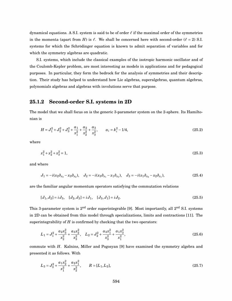
dynamical equations. A S.I. system is said to be of order ` if the maximal order of the symmetries
in the momenta (apart from H) is `. We shall be concerned here with second-order (` = 2) S.I.
systems for which the Schrödinger equation is known to admit separation of variables and for
which the symmetry algebras are quadratic.
S.I. systems, which include the classical examples of the isotropic harmonic oscillator and of
the Coulomb-Kepler problem, are most interesting as models in applications and for pedagogical
purposes. In particular, they form the bedrock for the analysis of symmetries and their descrip-
tion. Their study has helped to understand how Lie algebras, superalgebras, quantum algebras,
polynomials algebras and algebras with involutions serve that purpose.
25.1.2 Second-order S.I. systems in 2D
The model that we shall focus on is the generic 3-parameter system on the 2-sphere. Its Hamilto-
nian is
H = J21 + J2
2 + J23 + a1
x21+ a2
x22+ a3
x23
, ai = k2i −1/4, (25.2)
where
x21 + x2
2 + x23 = 1, (25.3)
and where
J1 =−i(x2∂x3 − x3∂x2), J2 =−i(x3∂x1 − x1∂x3), J3 =−i(x1∂x2 − x2∂x1), (25.4)
are the familiar angular momentum operators satisfying the commutation relations
[J1, J2]= iJ3, [J2, J3]= iJ1, [J3, J1]= iJ2. (25.5)
This 3-parameter system is 2nd order superintegrable [9]. Most importantly, all 2nd S.I. systems
in 2D can be obtained from this model through specializations, limits and contractions [11]. The
superintegrability of H is confirmed by checking that the two operators:
L1 = J21 + a2x2
3
x22
+ a3x22
x23
, L2 = J22 + a3x2
1
x23
+ a1x23
x21
, (25.6)
commute with H. Kalnins, Miller and Pogosyan [9] have examined the symmetry algebra and
presented it as follows. With
L3 = J23 + a1x2
2
x21
+ a2x21
x22
, R = [L1,L2], (25.7)
594

one has [H,L3]= 0, H = L1 +L2 +L3 +a1 +a2 +a3, and the relations (with (i jk) cyclic)
[L i,R]= 4L i,L j−4L i,Lk− (8−16a j)L j + (8−16ak)Lk +8(a j −ak), (25.8a)
R2 =− 83
L1,L2,L3−3∑
i=1
(12−16ai)L2
i +13
(16−176ai)L i + 323
ai
+ 52
3(L1,L2+ L2,L3+ L1,L3)+48(a1a2 +a2a3 +a3a1)
−64a1a2a3,
(25.8b)
where A,B = AB +BA. Remarkably, Kalnins, Miller and Post [10] have further shown that
the quadratic symmmetry algebra can be realized in terms of the difference operators associated
to the Racah polynomials, that these same polynomials occur as transition coefficients between
bases in which L1 or L2 is diagonal and furthermore that contractions of representations of the
symmetry algebra lead to the symmetry algebras of the other 2nd order S.I. systems and other
families of orthogonal polynomials [11]. Details about these Racah polynomials [12], denoted by
Rn(λ(x);α,β,γ,δ), will be given later. Suffice it to say for now that they are defined in terms of
generalized hypergeometric functions, that they are of degree n in the variable λ(x)= x(x+γ+δ+1),
that they obey a discrete/finite orthogonality relation and that they sit atop the discrete part of
the Askey scheme of hypergeometric orthogonal polynomials [12].
25.1.3 Objectives
In reduced form, the (quadratic) Racah algebra has three generators K1, K2, K3 and the defining
relations
[K1,K2]= K3,
[K2,K3]= K22 + K1,K2+dK2 + e1, (25.9)
[K3,K1]= K21 + K1,K2+dK1 + e2,
where d, e1 and e2 are real parameters. The objectives of this paper are to show that this algebra
has a universal character and intimately connects the generic second-order S.I. system on S2, the
Racah polynomials and the recoupling of three su(1,1) representations. Schematically, the goal is
595
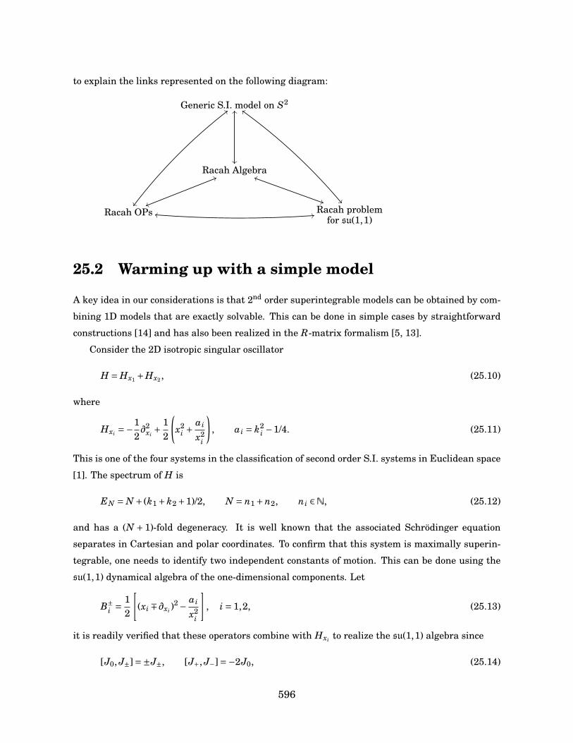
to explain the links represented on the following diagram:
Generic S.I. model on S2OO
Racah Algebra55
uu
ii
))
Racah OPs
;;
nn 00 Racah problemfor su(1,1)
dd
25.2 Warming up with a simple model
A key idea in our considerations is that 2nd order superintegrable models can be obtained by com-
bining 1D models that are exactly solvable. This can be done in simple cases by straightforward
constructions [14] and has also been realized in the R-matrix formalism [5, 13].
Consider the 2D isotropic singular oscillator
H = Hx1 +Hx2 , (25.10)
where
Hxi =−12∂2
xi+ 1
2
(x2
i +ai
x2i
), ai = k2
i −1/4. (25.11)
This is one of the four systems in the classification of second order S.I. systems in Euclidean space
[1]. The spectrum of H is
EN = N + (k1 +k2 +1)/2, N = n1 +n2, ni ∈N, (25.12)
and has a (N + 1)-fold degeneracy. It is well known that the associated Schrödinger equation
separates in Cartesian and polar coordinates. To confirm that this system is maximally superin-
tegrable, one needs to identify two independent constants of motion. This can be done using the
su(1,1) dynamical algebra of the one-dimensional components. Let
B±i = 1
2
[(xi ∓∂xi )
2 − ai
x2i
], i = 1,2, (25.13)
it is readily verified that these operators combine with Hxi to realize the su(1,1) algebra since
[J0, J±]=±J±, [J+, J−]=−2J0, (25.14)
596
with
J0 = Hxi /2 and J± = B±i /2.
In the positive-discrete series of su(1,1) representations thus constructed, B±i act as raising and
lowering operators with respect to the eigenvalues of Hxi labeled by ni. The conserved quantities
of the 2D Hamiltonian H = Hx1 + Hx2 are readily obtained from this observation. Indeed, com-
bining the raising operator for Hx1 with the lowering operator for Hx2 (or vice-versa) will give
an operator that leaves the total energy EN unchanged and that commutes with H. This is a
straightforward generalization of the Schwinger construction for the isotropic harmonic oscillator.
The superintegrability of H is thus made manifest by exhibiting the operators
C+ = B+x1
B−x2
, C− = B−x1
B+x2
, (25.15)
to which we conveniently add
D = Hx1 −Hx2 , (25.16)
and by noting that
[H,C±]= 0, [H,D]= 0. (25.17)
Defining relations for the symmetry algebra formed by the operators C± and D are straightfor-
wardly obtained [14]:
[D,C±]=±4C±,
[C−,C+]= D3 +α1D+α2,(25.18)
where
α1 =−H2 −2(k21 +k2
2 −2), α2 = (2k21 −2k2
2)H. (25.19)
Since H is central, α1 and α2 can be treated as constants on eigenspaces of H. An algebraic
solution of the problem is obtained by working out the appropriate representations of this algebra.
A special case of (25.18) was found by Higgs in [7] as symmetry algebra of the Coulomb problem
on S2. By taking a different set of operators, it is possible to cast the relations (25.18) in a form
that we would say is standard. Let
K1 = 18
(Hx1 −Hx2
), K2 = 1
8
(C++C−+ 1
2(D2 −H2)
). (25.20)
It is seen that K2 can be written as
K2 = 18
((x1∂x2 − x2∂x1)2 − a1x2
2
x21
− a2x21
x22
−1/2
), (25.21)
597
and is purely angular in polar coordinates. If we take
K3 = [K1,K2]= 116
(C+−C−), (25.22)
the defining relations become
[K1,K2]= K3,
[K2,K3]= K1,K2+δ1K1 +δ2,
[K3,K1]= K21 −
14
K2 +δ3,
(25.23)
with
δ1 =−14
(k21 +k2
2 −2), δ2 = 132
(k1 −k2)(k1 +k2)H, δ3 =− 164
H2. (25.24)
This presentation allows the identification with the Hahn algebra, a special case of the “generic"
Racah algebra (see next section). It is known to appear in connection with the Clebsch-Gordan
problem for su(1,1) [17]. This suggests a potential link between the isotropic singular oscillator in
two dimensions and the Clebsch-Gordan problem for the dynamical algebra of its one-dimensional
components. We shall now proceed to discuss the most general second order S.I. model in two
dimensions along the lines followed in this section and shall see that the link mentioned above
is not fortuitous. However before we do so, we shall introduce thoroughly the Racah algebra,
present its finite-dimensional representations and go over the relations these have with Racah
polynomials.
25.3 The Racah algebra
The Racah algebra has three generators K1, K2 and K3. In the generic presentation, they obey
the relations
[K1,K2]= K3,
[K2,K3]= a2K22 +a1K1,K2+ c1K1 +dK2 + e1,
[K3,K1]= a1K21 +a2K1,K2+ c2K2 +dK1 + e2,
(25.25)
where the parameters a1, a2, c1, c2, d, e1 and e2 are taken to be real. This defines the most
general associative quadratic algebra with two independent generators and a ladder property.
To see this, let K1, K2 be the two independent generators and define [K1,K2] = K3. K1 and K2
are assumed to be Hermitian, K3 is thus anti-Hermitian. Consider the most general quadratic
relations compatible with the hermiticity conditions:
[K2,K3]= a2K22 +a1K1,K2+ g1K2
1 +h1K23 + c1K1 +d1K2 + e1,
[K3,K1]= a3K21 +a4K1,K2+ g2K2
2 +h2K23 + c2K2 +d2K1 + e2.
(25.26)
598
It follows from the Jacobi identity
[K1, [K2,K3]]+ [K3, [K1,K2]]+ [K2, [K3,K1]]= 0,
that
d1 = d2, a3 = a1, a4 = a2, h1 = h2 = 0. (25.27)
One then requires g1 = g2 = 0 to ensure the ladder property (see later) and thus recovers (25.25).
This algebra made its appearance in the work of Granovskii and Zhedanov [3] where it was used
in the context of the Racah problem of su(2) to derive the symmetry group of the 6 j-symbols. It is
also known as the Racah-Wilson algebra. When neither a1 nor a2 are zero, that is when a1 ·a2 6= 0,
the relations can be put in the following canonical form
[K1,K2]= K3, (25.28a)
[K2,K3]= K22 + K1,K2+dK2 + e1, (25.28b)
[K3,K1]= K21 + K1,K2+dK1 + e2, (25.28c)
where d, e1 and e2 are still real. This presentation thus retains three essential structure parame-
ters and is arrived at by simple affine transformations of the generators K i → uiK i +vi, i = 1,2,3.
It is verified that this algebra has the following Casimir operator (central element)
Q =K21 ,K2+ K1,K2
2+K21 +K2
2 +K23
+ (d+1)K1,K2+ (2e1 +d)K1 + (2e2 +d)K2,(25.29)
which is cubic in the generators and commutes with each one of them.
25.4 Representations of the Racah algebra and Racah
polynomials
We now wish to point out the connection between the Racah algebra and the Racah orthogonal
polynomials. This can be done in at least two ways:
1. By constructing the finite-dimensional representations of the algebra.
2. By realizing the algebra in terms of the operators associated to the polynomials.
We shall describe these two approaches in the following. We shall begin this section though by
registering the basic definitions and properties of the Racah polynomials that we shall use.
599
25.4.1 Racah polynomials
The Racah polynomials Rn(λ(x);α,β,γ,δ) of degree n in λ(x) = x(x+γ+δ+1) depend on four real
parameters α, β, γ, δ and are defined by the following explicit expression (n ∈N):
Rn(λ(x))= 4F3
[−n,n+α+β+1,−x, x+γ+δ+1α+1,β+δ+1,γ+1
;1], (25.30)
where pFq is the generalized hypergeometric series
pFq
a1 · · · ap
b1 · · · bq; z
=∞∑j=0
(a1) j · · · (ap) j
(b1) j · · · (bq) j
z j
j!, (25.31)
and
(a) j = a(a+1) · · · (a+ j−1).
The series in (25.30) truncates since (−n) j = 0 for j > n+1. The polynomials thus defined satisfy
R0(λ(x))= 1 and a three-term recurrence relation of the form [12]
λ(x)Rn(λ(x))= AnRn+1(λ(x))− (An +Cn)Rn(λ(x))+CnRn−1(λ(x)), (25.32)
with
An = (n+α+1)(n+α+β+1)(n+β+δ+1)(n+γ+1)(2n+α+β+1)(2n+α+β+2)
,
Cn = n(n+α+β−γ)(n+α−δ)(n+β)(2n+α+β)(2n+α+β+1)
.(25.33)
As usual it is assumed that R−1(λ(x)) = 0. Like all polynomials of the Askey scheme, the Racah
polynomials are bispectral: in addition to obeying the above recurrence relation, they are aso
eigenfunctions of the difference equation
L Rn(λ(x))= n(n+α+β+1)Rn(λ(x)), (25.34)
where
L = B(x)T++D(x)T−− (B(x)+D(x))I, (25.35)
with
T± f (x)= f (x±1), (25.36)
and
B(x)= (x+α+1)(x+β+δ+1)(x+γ+1)(x+γ+δ+1)(2x+γ+δ+1)(2x+γ+δ+2)
,
D(x)= x(x−α+γ+δ)(x−β+γ)(x+δ)(2x+γ+δ)(2x+γ+δ+1)
.(25.37)
600
Provided one of the following truncation conditions holds:
α+1=−N, β+δ+1=−N, γ+1=−N,
the Racah polynomials Rn(λ(x)) enjoy a finite orthogonality relation of the form
N∑x=0
wxRn(λ(x))Rm(λ(x))= hnδnm, (25.38)
where wx and hn are known explicitly. (For more details on the Racah polynomials see [12] where
in particular the limit relations to other OPs of the Askey scheme are provided.)
25.4.2 Finite-dimensional representations
We shall now describe the finite-dimensional unitary representations of the Racah algebra and
sketch how they are obtained. We take the defining relations to be in the canonical form (25.28).
We begin by taking one generator, say K1, to be diagnal on the representation space and proceed
to show that the Racah algebra has a ladder property.
Let ωp be a vector of the representation space such that
K1ωp =λpωp, p ∈R. (25.39)
Suppose we look for another eigenvector ωp′ with eigenvalue λp′ that has the form
ωp′ = α(p)K1 +β(p)K2 +γ(p)K3
ωp, (25.40)
where α(p), β(p) and γ(p) are coefficients. Imposing the eigenvalue equation
K1ωp′ =λp′ωp′ , (25.41)
using (25.39) and the commutation relations (25.28a) and (25.28c), it is seen that the eigenvalues
λp′ must satisfy
(λp′ −λp)2 + (λp′ +λp)= 0. (25.42)
For a given λp, there are two solutions which we can choose to call λp+1 and λp−1. Assuming that
λp is non-degenerate and denoting by Eλp the one-dimensional eigenspace, it follows from the
above considerations that a generic element of the algebra will map Eλp onto Eλp−1 ⊕Eλp ⊕Eλp+1 .
We can thus write
K1ωp =λpωp,
K2ωp =Up+1ωp1 +Vpωp +Upωp−1,
K3ωp = [K1,K2]ωp =Up+1 gp+1ωp+1 −Up gpωp−1,
(25.43)
601

with
gp =λp −λp−1, (25.44)
observing that K2 is tridiagonal and K3 bidiagonal. Note that K2 is self-adjoint if Up is real.
Having understood that the representations of the Racah algebra have a ladder structure, we now
wish to focus on those representations that are finite-dimensional and for which the spectrum of
K1 is discrete. In the following we shall hence replace the vectors ωp, p ∈ R, by the vectors ψn,
n ∈Z, labeled by the discrete index n. The actions (25.43) become
K1ψn =λnψn,
K2ψn =Un+1ψn+1 +Vnψn +Unψn−1,
K3ψn =Un+1 gn+1ψn+1 −Un gnψn−1.
(25.45)
with
gn =λn −λn−1, (25.46)
and there remains to determine λn, Vn and Un. From (25.28c), one finds
λn = (σ−n)(n−σ+1)/2, gn =σ−n, (25.47)
and
Vn =−λ2n +dλn + e2
λn, (25.48)
where σ is an arbitrary real parameter. We observe that the spectrum is quadratic in n. To find
Un, one uses (25.28b) that yields the following recurrence relation for U2n:
2(gn+3/2U2n+1 − gn−1/2U2
n)=V 2n + (2λn +d)Vn + e1. (25.49)
Instead of solving directly (25.49), it is simpler to use the fact that the Casimir operator Q given
in (25.29) is constant on irreducible representation spaces in order to find an expression for
2(gn+3/2 gnU2n+1 + gn+1 gn−1/2U2
n).
Upon eliminating Un+1 with the help of this result and solving (25.49) for U2n one arrives at
U2n = P (g2
n)64g2
n gn−1/2 gn+1/2, (25.50)
where P (z) is the fourth degree polynomial
P (z)=z4 − (4d+2)z3 + (4d2 +4d+1+8e2 −16e1)z2
−4(d2 +2e2 +4de2 +4q)z+16e22.
(25.51)
602
In terms of the roots ξ2k of P (g2
n), we can write
U2n =
∏4k=1(g2
n −ξ2k)
64g2n gn−1/2 gn+1/2
. (25.52)
For finite-dimensional representations, the index n is comprised in a finite interval N1 ≤ n ≤ N2,
N1, N2 ∈Z and the eigenvalues of K1 are λN1 ,λN1+1, . . . ,λN2 . Setting the arbitrary parameter σ in
(25.47) equal to N1 +ρ and calling N = N2 −N1, we can equivalently restrict the label n to be in
the interval
0≤σ≤ N, (25.53)
with the eigenvalues λ0, λ1, . . . ,λN given by
λn = (ρ−n)(n−ρ+1)/2. (25.54)
Clearly, in a (N+1)-dimensional representation we must have U0 =UN+1 = 0 so that ψ−1 and ψN+1
cannot be reached by the actions of K2 on ψ0 and ψN , respectively. This will be observed if one of
the zeros ξ2k, k = 1,2,3,4, say ξ2
i is such that
ξ2i = g2
0 = ρ2, (25.55a)
and another say ξ2j , verify
ξ2j = g2
N+1 = (ρ−N −1)2. (25.55b)
25.4.3 Connection with Racah polynomials
Having described the finite-dimensional representations of the Racah algebra in the eigenbasis of
K1, we might wonder what the picture is in the eigenbasis of K2. It turns out to be very similar.
Indeed, it is observed that the defining relations (25.28) are invariant under the exchanges
K1 ↔ K2, e1 ↔ e2. (25.56)
It follows that the representation in the bases φs in which K2 is diagonal
K2φs =µsφs, (25.57)
can be obtained from those in which K1 is diagonal using this symmetry property. In this corre-
spondence with the formulas of the last subsection, we make the replacement n → s. It is clear
that µs will have a from similar to λn say
µs = (ν− s)(ν− s+1)/2, (25.58)
603
and that K1 will be tridiagonal in the φs basis. In other words, K1 and K2 realize a Leonard pair
[15]. We now claim that the Racah polynomials arise as overlaps between the ψn and the φs
bases; that is, the Racah polynomials appear as expansion coefficients between the basis in which
K1 is diagonal and the one in which K2 is diagonal.
Let us make this more explicit. Since the bases φs and ψn span isomorphic spaces we can
expand the elements of one in terms of those of the other:
φs =N∑
n=0Wn(s)ψn. (25.59)
Let us write the coefficients Wn(s) in the form
Wn(s)= w0(s)Pn(µs), (25.60)
so that P0(µs)= 1. Using (25.57) and (25.45), it is seen upon acting with K2 on both sides of (25.59)
that the quantities Pn(µs) obey
µsPn(µs)=Un+1Pn+1(µs)+VnPn(µs)+UnPn−1(µs). (25.61)
Given the formulas for Un and Vn, this recurrence relation is seen to coincide with that of the
Racah polynomials. The zeros ξ2k are related to the parameters α,β,γ,δ of the polynomials
Rn(λ(x);α,β,γ,δ). If the truncations conditions are satisfied through
ξ1 = ρ, ξ4 = (ρ−N −1), (25.62)
(recall (25.55)) the identification is achived by the following parametrization of the roots:
ξ1 =−α+β2
, ξ2 = β−α2
+δ, ξ3 = β−α2
, ξ4 = γ− α+β2
. (25.63)
25.4.4 The Racah algebra from the Racah polynomials
We have illustrated how the Racah polynomials can be obtained from the Racah algebra by con-
structing the finite-dimensional representations. Let us indicate now that conversely, the Racah
algebra can be identified from the properties of the Racah polynomials. As shall be seen the Racah
algebra encodes the bispectrality properties of the polynomials. These properties amount to the
fact that in addition to satisfying a three-term recurrence relation (as all orthogonal polynomials
must do), the Racah polynomials also obey a difference equation. Let us recall that these relations
can be put in the form
x(x+γ+δ+1)Rn(λ(x))=M Rn(λ(x)), (25.64a)
L Rn(λ(x))= n(n+α+β+1)Rn(λ(x)), (25.64b)
604
where the recurrence operator M and the difference operator L are given by
M = AnT+n +CnT−
n − (An +Cn)I, (25.65)
L = B(x)T+x +D(x)T−
x − (B(x)+D(x))I, (25.66)
with T±n f (n) = f (n±1), T±
x f (x) = f (x±1) and where An, Cn are given in (25.33) and B(x), D(x)
provided by (25.37). Consider now the realization on functions of x, where K1 and K2 are the two
operators occurring on the left-hand side of (25.64), i.e. K1 is the recurrence operator and K2 is
the difference operator:
K1 = x(x+γ+δ+1), K2 =L . (25.67)
Performing the affine transformations
K1 = u1K1 +v1, K2 = u2K2 +v2, (25.68)
one finds that K1, K2 verify the Racah algebra relations (25.28) with
e1 = 14
(α−β
2
)(α+β
2
)(α+β
2−γ
)(α−β
2−δ
),
e2 = 14
(γ−δ
2
)(γ+δ
2
)(γ+δ
2−α
)(γ−δ
2−β
),
d = 14
(γ−δ
2
)2+
(γ+δ
2
)2+
(γ+δ
2−α
)2+
(γ−δ
2−β
)2−2
.
We could obviously have taken the realization on functions of n with
K1 =M , K2 = n(n+α+β+1), (25.69)
which is bound to lead to the same algebra. The duality property of the Racah polynomials under
the exchanges
x ↔ n, α↔ γ, β↔ δ, (25.70)
which follows from (25.64) is immediately seen to correspond to the symmetry of the Racah algebra
under
K1 ↔ K2, K3 ↔−K3, e1 ↔ e2, (25.71)
that we already observed.
605
25.5 The generic superintegrable model on S2 and
su(1,1)
We now return to the generic superintegrable model on S2 with Hamiltonian (25.2) and constants
of motion (25.6) and (25.7). We want to show that it is intimately connected to the su(1,1) algebra.
Consider three su(1,1) realizations identical to the one introduced in the discussion of the
two-dimensional singular oscillator in Section 2:
J(i)0 = 1
4
(−∂2
xi+ x2
2 +ai
x2i
), J(i)
± = 14
((xi ∓∂xi )
2 − ai
x2i
), (25.72)
with ai = k2i −1/4 and i = 1,2,3. These provide positive discrete series representations for which
the su(1,1) Casimir element
C(i) = [J(i)0 ]2 − J(i)
+ J(i)− − J(i)
0 , i = 1,2,3, (25.73)
takes the value
C(i) = νi(νi −1), νi = (ki +1)/2. (25.74)
These three sets of su(1,1) generators can be added to produce a “fourth” realization:
J(4)0 = J(1)
0 + J(2)0 + J(3)
0 , J(4)± = J(1)
± + J(2)± + J(3)
± . (25.75)
Three types of Casimir operators can be distinguished in the process:
1. The “initial” Casimir operators (25.73)
2. The “intermediate” Casimir operators associated to the addition of two representations
C(i j) = [J(i)0 + J( j)
0 ]2 − (J(i)+ + J( j)
+ )(J(i)− + J( j)
− )− (J(i)0 + J( j)
0 ), (25.76)
with (i j)= (12), (23), (31).
3. The “full” Casimir operator
C(4) = [J(4)0 ]2 − J(4)
+ J(4)− − J(4)
0 . (25.77)
By a direct computation one finds that
C(i j) = 14
J2
k +aix2
j
x2i
+ a jx2i
x2j
+ai +a j −1
, (25.78)
606
with (i jk) a cyclic permutation of (1,2,3). Comparing with (25.6) and (25.7), we see that
L1 = 4C(23) −a2 −a3 +1, L2 = 4C(31) −a3 −a1 +1, L3 = 4C(12) −a1 −a2 +1, (25.79)
and thus observe that the constants of motion of the generic S.I. system on S2 are basically the
intermediate Casimir operators arising in the addition of three su(1,1) representations. Similarly
one can check that the full Casimir operator C(4) takes the following form when (25.72) and (25.75)
are used in (25.77):
C(4) = 14
J2
1 + J22 + J2
3 + (x21 + x2
2 + x23)
(a1
x21+ a2
x22+ a3
x23
)− 3
4
. (25.80)
As a consequence,
H = 4C(4) + 34
, (25.81)
if x21+ x2
2+ x23 = 1. At this point we may ask if this restriction to S2 can generally be ensured in the
addition of the three su(1,1) representations. That the answer is yes is readily seen. It is noted
from (25.72) that
2J(i)0 + J(i)
+ + J(i)− = x2
i , (25.82)
and hence that
S = 2J(4)0 + J(4)
+ + J(4)− = x2
1 + x22 + x2
3. (25.83)
Since S commutes with 4C(4) + 3/4, it is “time-independent” and as a constant can be taken to
be 1. We can thus conclude the following. The generic S.I. 3-paramater system is obtained from
the addition of three su(1,1) realizations. In this identification the restriction x21 + x2
2 + x23 = 1 to
S2 is preserved; the Hamiltonian corresponds to the full Casimir operator C(4) for the addition
of the three representations and the constants of motion are obviously the intermediate Casimir
operators C(i j) which commute with C(4). The algebra that these intermediate Casimir operators
generate is thus the symmetry algebra of the generic S.I. system on S2. We shall show in the
next section that the intermediate Casimir operators in the addition of three su(1,1) irreducible
representations generate the Racah algebra.
Note that the R-matrix approach has been used in [6] to describe the generic 3-parameter
model on S2 and construct its invariants. One proceeds via dimensional reduction from S5 to S2
with a Lax matrix that also involves three su(1,1) elements. It is interesting to further point out
that the same generic S.I. model on S2 has been shown to correspond to one of the Krall-Sheffer
classes of orthogonal polynomials in two variables [4, 16].
607
25.6 The Racah problem for su(1,1) and
the Racah algebra
We loosely refer to the Racah problem as the recoupling of three irreducible representations.
Strictly speaking, it is about determining the unitary transformation between two canonical bases
corresponding to the steps (1⊕2)⊕3 and 1⊕ (2⊕3) which are respectively associated to the di-
agonalization of the intermediate Casimir operators C(12) and C(23). Our goal in this section is
to comment on the algebra that C(12) and C(23) generate in the case of su(1,1) (and of su(2) as a
matter of fact).
Consider the addition of three su(1,1) representations as in (25.75) and take each initial
Casimir operator C(i) to be a multiple of the identity:
C(i) =λi, i = 1,2,3. (25.84)
The intermediate Casimir operators C(12) and C(23) (given by (25.76)) can then be expressed as
follows
C(12) = 2J(1)0 J(2)
0 − (J(1)+ J(2)
− + J(1)− J(2)
+ )+λ1 +λ2,
C(23) = 2J(2)0 J(3)
0 − (J(2)+ J(3)
− + J(2)− J(3)
+ )+λ2 +λ3.(25.85)
Further assume that the full Casimir operator C(4) which can be written in the form
C(4) = C(12) +C(23) +C(31) −C(1) −C(2) −C(3), (25.86)
is also a multiple of the identity, i.e.
C(4) =λ4. (25.87)
Denoting by V (λi) an irreducible su(1,1) representation space on which the Casimir operator C(i)
is equal to λi, we are thus looking at the decomposition of V (λ1) ⊗V (λ2) ⊗V (λ3) in irreducible com-
ponents V (λ4). Consider now the algebra generated by the intermediate Casimir operators in this
Racah problem. Define
κ1 =−C(12)/2 κ2 =−C(23)/2, (25.88)
and let
κ3 = [κ1,κ2]. (25.89)
608
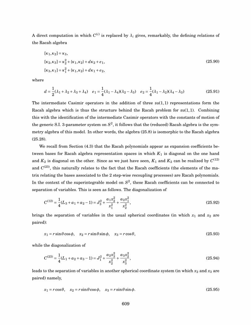
A direct computation in which C(i) is replaced by λi gives, remarkably, the defining relations of
the Racah algebra
[κ1,κ2]= κ3,
[κ2,κ3]= κ22 + κ1,κ2+dκ2 + e1,
[κ3,κ1]= κ21 + κ1,κ2+dκ1 + e2,
(25.90)
where
d = 12
(λ1 +λ2 +λ3 +λ4) e1 = 14
(λ1 −λ4)(λ2 −λ3) e2 = 14
(λ1 −λ2)(λ4 −λ3) (25.91)
The intermediate Casimir operators in the addition of three su(1,1) representations form the
Racah algebra which is thus the structure behind the Racah problem for su(1,1). Combining
this with the identification of the intermediate Casimir operators with the constants of motion of
the generic S.I. 3-parameter system on S2, it follows that the (reduced) Racah algebra is the sym-
metry algebra of this model. In other words, the algebra (25.8) is isomorphic to the Racah algebra
(25.28).
We recall from Section (4.3) that the Racah polynomials appear as expansion coefficients be-
tween bases for Racah algebra representation spaces in which K1 is diagonal on the one hand
and K2 is diagonal on the other. Since as we just have seen, K1 and K2 can be realized by C(12)
and C(23), this naturally relates to the fact that the Racah coefficients (the elements of the ma-
trix relating the bases associated to the 2 step-wise recoupling processes) are Racah polynomials.
In the context of the superintegrable model on S2, these Racah coefficients can be connected to
separation of variables. This is seen as follows. The diagonalization of
C(12) = 14
(L3 +a1 +a2 −1)= J23 + a1x2
2
x21
+ a2x21
x22
, (25.92)
brings the separation of variables in the usual spherical coordinates (in which x1 and x2 are
paired):
x1 = rsinθ cosφ, x2 = rsinθsinφ, x3 = r cosθ, (25.93)
while the diagonalization of
C(23) = 14
(L1 +a2 +a3 −1)= J21 + a2x2
3
x22
+ a3x22
x23
, (25.94)
leads to the separation of variables in another spherical coordinate system (in which x2 and x3 are
paired) namely,
x1 = r cosθ, x2 = rsinθ cosφ, x3 = rsinθsinφ. (25.95)
609

Hence the Racah polynomials are in this framework, the overlap coefficients between these two
sets of wavefunctions of the generic 3-parameter system on S2 which are obtained by separating
the variables in the considered systems (25.93) and (25.95).
Summing up, the identification of the generic S.I. model on S2 as the full Casimir operator
in the addition of three su(1,1) realizations provides a natural way of obtaining the constants of
motion (as the intermediate Casimir operators) and of determining the symmetry algebra (as the
Racah algebra). This intimately associates the Racah polynomials to the model on S2. It should
be said that representations with continuous spectra are found to bring the Wilson polynomials
in the picture. As explained in [11], all the other second order S.I. mdels in two dimensions can
be obtained from the generic system on S2 by contractions and specializations. Correspondingly,
when effected on the Racah algebra and the Racah/Wilson polynomials these operations provide
the symmetry algebras of all these second order S.I. models and their tagging to orthogonal poly-
nomials of the Askey scheme.
25.7 Conclusion
Let us summarize the main findings and offer perspectives. We presented the Racah algebra and
its finite-dimensional representations. We proceeded to explain its universal character and the
relations depicted on the diagram presented in Section I. It was shown that the Racah algebra is
behind
• The generic 3-parameter superintegrable model on S2 and hence all second order superin-
tegrable systems in two dimensions
• The Racah problem for su(1,1), that is the combination of three irreducible su(1,1) repre-
sentations
• The Racah polynomials that sit atop the discrete part of the Askey scheme of hypergeometric
orthogonal polynomials
Looking at three and higher dimensions, the analogous connections between superintegrable mod-
els, polynomial algebras and special functions are bound to be illuminating. They are expected to
feed the theory of multivariate orthogonal polynomials and their algebraic interpretations.
As an illustration of this, let us mention that Kalkins, Miller and Post have already shown that
2-variable Racah-Wilson polynomials occur in the S3 model [8]. The construction presented here
extends to any dimensions and the three-dimensional model on S3 arises from the addition of four
su(1,1) representations and corresponds to the 9 j or Fano problem for su(1,1). The symmetries in
this case are expected to lead to a rank 2 version of the Racah algebra which should encode the
610
properties of the general bivariate Racah-Wilson polynomials. We intend to pursue investigations
along those lines.
References
[1] J. Fris, V. Mandrosov, Ya. A. Smorodinsky, M. Uhlir, and P. Winternitz. On higher symmetries
in quantum mechanics. Phys. Lett., 16:354–356, 1965.
[2] V.X. Genest, L. Vinet, and A. Zhedanov. Superintegrability in two dimensions and the Racah-
Wilson algebra. ArXiv:1307.5539, 2013.
[3] Ya. A. Granovskii and A. Zhedanov. Nature of the symmetry group of the 6 j-symbol. Zh.
Eksp. Teor. Fiz., 94:49–54, 1988.
[4] J. Harnad, L. Vinet, O. Yermolayeva, and A. Zhedanov. Two-dimensional Krall-Sheffer poly-
nomials and integrable systems. J. Phys. A: Math. Gen., 34:10619, 2001.
[5] J. Harnad and O. Yermolayeva. Superintegrability, Lax matrices and separation of variables.
In CRM Proc. Lecture Notes.
[6] J. Harnad, A. Zhedanov, and O. Yermolayeva. R-Matrix Approach to the Krall-Sheffer Prob-
lem. Proc. Inst. Math. Nat. Acad. Sc. Ukr., 439:314–320, 2002.
[7] P. W. Higgs. Dynamical symmetries in a spherical geometry. I. J. Phys. A: Math. Gen.,
12(3):309, 1979.
[8] E. G. Kalnins, W. Miller, and S. Post. Two-variable Wilson polynomials and the generic
superintegrable system on the 3-sphere. SIGMA, 7:51–76, 2011.
[9] E.G. Kalnins, W. Miller, and G. S. Pogosyan. Superintegrability and associated polynomial
solutions: Euclidean space and the sphere in two dimensions. J. Math. Phys., 37:6439, 1996.
[10] E.G. Kalnins, W. Miller, and S. Post. Wilson polynomials and the generic superintegrable
system on the 2-sphere. J. Phys. A: Math. Theor., 40:11525–11538, 2007.
[11] E.G. Kalnins, W. Miller, and S. Post. Contractions of 2D 2nd order quantum superintegrable
systems and the Askey scheme for hypergeometric orthogonal polynomials. SIGMA, 9:57–84,
2013.
[12] R. Koekoek, P.A. Lesky, and R.F. Swarttouw. Hypergeometric orthogonal polynomials and
their q-analogues. Springer, 1st edition, 2010.
611
[13] V. Kuznetsov. Quadrics on real Riemannian spaces of constant curvature: separation of
variables and connection with Gaudin magnet. J. Math. Phys., 33:1992, 3240.
[14] P. Letourneau and L. Vinet. Superintegrable Systems: Polynomial Algebras and Quasi-
Exactly Solvable Hamiltonians. Ann. Phys., 243:144–168, 1995.
[15] P. Terwilliger. Two linear transformations each tridiagonal with respect to an eigenbasis of
the other. Lin. Alg. Appl., 330:149–203, 2001.
[16] L. Vinet and A. Zhedanov. Two-Dimensional Krall–Sheffer Polynomials and Quantum Sys-
tems on Spaces with Constant Curvature. Lett. Math. Phys, 65:83–94, 2003.
[17] A. Zhedanov. Hidden symmetry algebra and overlap coefficients for two ring-shaped poten-
tials. J. Phys. A: Math. Gen., 26(18):4633, 1993.
612
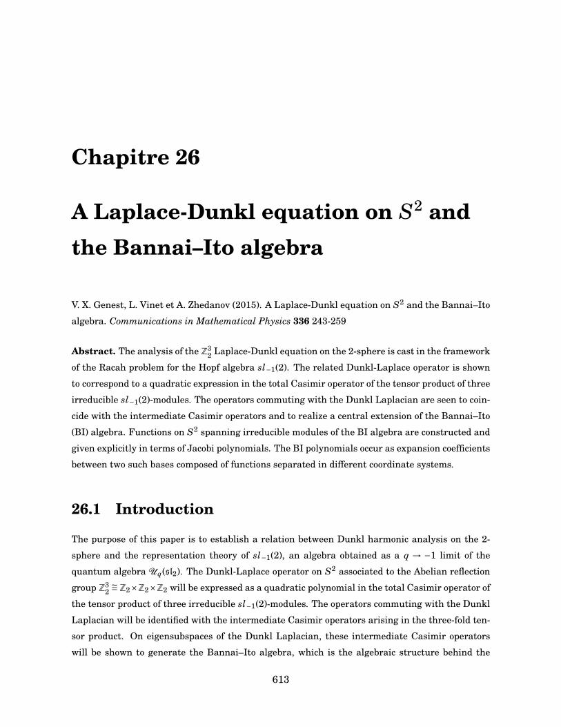
Chapitre 26
A Laplace-Dunkl equation on S2 andthe Bannai–Ito algebra
V. X. Genest, L. Vinet et A. Zhedanov (2015). A Laplace-Dunkl equation on S2 and the Bannai–Ito
algebra. Communications in Mathematical Physics 336 243-259
Abstract. The analysis of the Z32 Laplace-Dunkl equation on the 2-sphere is cast in the framework
of the Racah problem for the Hopf algebra sl−1(2). The related Dunkl-Laplace operator is shown
to correspond to a quadratic expression in the total Casimir operator of the tensor product of three
irreducible sl−1(2)-modules. The operators commuting with the Dunkl Laplacian are seen to coin-
cide with the intermediate Casimir operators and to realize a central extension of the Bannai–Ito
(BI) algebra. Functions on S2 spanning irreducible modules of the BI algebra are constructed and
given explicitly in terms of Jacobi polynomials. The BI polynomials occur as expansion coefficients
between two such bases composed of functions separated in different coordinate systems.
26.1 Introduction
The purpose of this paper is to establish a relation between Dunkl harmonic analysis on the 2-
sphere and the representation theory of sl−1(2), an algebra obtained as a q → −1 limit of the
quantum algebra Uq(sl2). The Dunkl-Laplace operator on S2 associated to the Abelian reflection
group Z32∼=Z2×Z2×Z2 will be expressed as a quadratic polynomial in the total Casimir operator of
the tensor product of three irreducible sl−1(2)-modules. The operators commuting with the Dunkl
Laplacian will be identified with the intermediate Casimir operators arising in the three-fold ten-
sor product. On eigensubspaces of the Dunkl Laplacian, these intermediate Casimir operators
will be shown to generate the Bannai–Ito algebra, which is the algebraic structure behind the
613
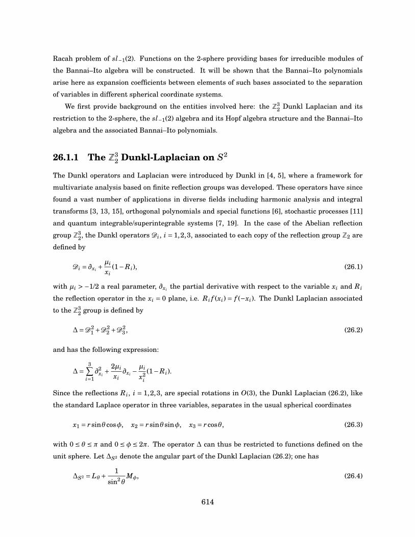
Racah problem of sl−1(2). Functions on the 2-sphere providing bases for irreducible modules of
the Bannai–Ito algebra will be constructed. It will be shown that the Bannai–Ito polynomials
arise here as expansion coefficients between elements of such bases associated to the separation
of variables in different spherical coordinate systems.
We first provide background on the entities involved here: the Z32 Dunkl Laplacian and its
restriction to the 2-sphere, the sl−1(2) algebra and its Hopf algebra structure and the Bannai–Ito
algebra and the associated Bannai–Ito polynomials.
26.1.1 The Z32 Dunkl-Laplacian on S2
The Dunkl operators and Laplacian were introduced by Dunkl in [4, 5], where a framework for
multivariate analysis based on finite reflection groups was developed. These operators have since
found a vast number of applications in diverse fields including harmonic analysis and integral
transforms [3, 13, 15], orthogonal polynomials and special functions [6], stochastic processes [11]
and quantum integrable/superintegrable systems [7, 19]. In the case of the Abelian reflection
group Z32, the Dunkl operators Di, i = 1,2,3, associated to each copy of the reflection group Z2 are
defined by
Di = ∂xi +µi
xi(1−Ri), (26.1)
with µi > −1/2 a real parameter, ∂xi the partial derivative with respect to the variable xi and Ri
the reflection operator in the xi = 0 plane, i.e. Ri f (xi) = f (−xi). The Dunkl Laplacian associated
to the Z32 group is defined by
∆=D21 +D2
2 +D23 , (26.2)
and has the following expression:
∆=3∑
i=1∂2
xi+ 2µi
xi∂xi −
µi
x2i
(1−Ri).
Since the reflections Ri, i = 1,2,3, are special rotations in O(3), the Dunkl Laplacian (26.2), like
the standard Laplace operator in three variables, separates in the usual spherical coordinates
x1 = rsinθ cosφ, x2 = rsinθsinφ, x3 = r cosθ, (26.3)
with 0 ≤ θ ≤ π and 0 ≤ φ ≤ 2π. The operator ∆ can thus be restricted to functions defined on the
unit sphere. Let ∆S2 denote the angular part of the Dunkl Laplacian (26.2); one has
∆S2 = Lθ+ 1sin2θ
Mφ, (26.4)
614
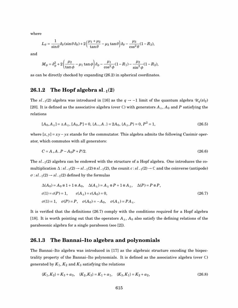
where
Lθ = 1sinθ
∂θ (sinθ∂θ)+2(µ1 +µ2
tanθ−µ3 tanθ
)∂θ− µ3
cos2θ(1−R3),
and
Mφ = ∂2φ+2
(µ2
tanφ−µ1 tanφ
)∂φ− µ1
cos2φ(1−R1)− µ2
sin2φ(1−R2),
as can be directly checked by expanding (26.2) in spherical coordinates.
26.1.2 The Hopf algebra sl−1(2)
The sl−1(2) algebra was introduced in [16] as the q → −1 limit of the quantum algebra Uq(sl2)
[20]. It is defined as the associative algebra (over C) with generators A±, A0 and P satisfying the
relations
[A0, A±]=±A±, [A0,P]= 0, A+, A−= 2A0, A±,P= 0, P2 = 1, (26.5)
where [x, y]= xy− yx stands for the commutator. This algebra admits the following Casimir oper-
ator, which commutes with all generators:
C = A+A−P − A0P +P/2. (26.6)
The sl−1(2) algebra can be endowed with the structure of a Hopf algebra. One introduces the co-
multiplication ∆ : sl−1(2)→ sl−1(2)⊗ sl−1(2), the counit ε : sl−1(2)→C and the coinverse (antipode)
σ : sl−1(2)→ sl−1(2) defined by the formulas
∆(A0)= A0 ⊗1+1⊗ A0, ∆(A±)= A±⊗P +1⊗ A±, ∆(P)= P ⊗P,
ε(1)= ε(P)= 1, ε(A±)= ε(A0)= 0, (26.7)
σ(1)= 1, σ(P)= P, σ(A0)=−A0, σ(A±)= P A±.
It is verified that the definitions (26.7) comply with the conditions required for a Hopf algebra
[18]. It is worth pointing out that the operators A±, A0 also satisfy the defining relations of the
parabosonic algebra for a single paraboson (see [2]).
26.1.3 The Bannai–Ito algebra and polynomials
The Bannai–Ito algebra was introduced in [17] as the algebraic structure encoding the bispec-
trality property of the Bannai–Ito polynomials. It is defined as the associative algebra (over C)
generated by K1, K2 and K3 satisfying the relations
K1,K2= K3 +α3, K2,K3= K1 +α1, K3,K1= K2 +α2, (26.8)
615
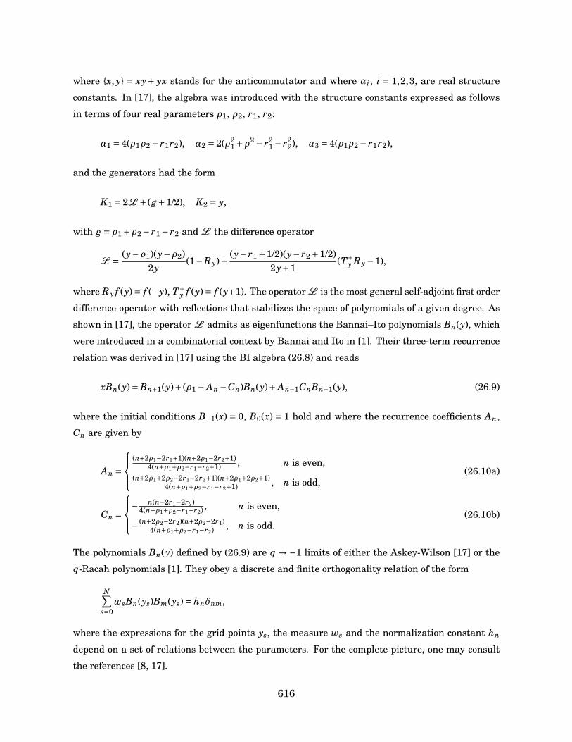
where x, y = xy+ yx stands for the anticommutator and where αi, i = 1,2,3, are real structure
constants. In [17], the algebra was introduced with the structure constants expressed as follows
in terms of four real parameters ρ1, ρ2, r1, r2:
α1 = 4(ρ1ρ2 + r1r2), α2 = 2(ρ21 +ρ2 − r2
1 − r22), α3 = 4(ρ1ρ2 − r1r2),
and the generators had the form
K1 = 2L + (g+1/2), K2 = y,
with g = ρ1 +ρ2 − r1 − r2 and L the difference operator
L = (y−ρ1)(y−ρ2)2y
(1−Ry)+ (y− r1 +1/2)(y− r2 +1/2)2y+1
(T+y Ry −1),
where Ry f (y)= f (−y), T+y f (y)= f (y+1). The operator L is the most general self-adjoint first order
difference operator with reflections that stabilizes the space of polynomials of a given degree. As
shown in [17], the operator L admits as eigenfunctions the Bannai–Ito polynomials Bn(y), which
were introduced in a combinatorial context by Bannai and Ito in [1]. Their three-term recurrence
relation was derived in [17] using the BI algebra (26.8) and reads
xBn(y)= Bn+1(y)+ (ρ1 − An −Cn)Bn(y)+ An−1CnBn−1(y), (26.9)
where the initial conditions B−1(x) = 0, B0(x) = 1 hold and where the recurrence coefficients An,
Cn are given by
An =
(n+2ρ1−2r1+1)(n+2ρ1−2r2+1)
4(n+ρ1+ρ2−r1−r2+1) , n is even,(n+2ρ1+2ρ2−2r1−2r2+1)(n+2ρ1+2ρ2+1)
4(n+ρ1+ρ2−r1−r2+1) , n is odd,(26.10a)
Cn =
− n(n−2r1−2r2)4(n+ρ1+ρ2−r1−r2) , n is even,
− (n+2ρ2−2r2)(n+2ρ2−2r1)4(n+ρ1+ρ2−r1−r2) , n is odd.
(26.10b)
The polynomials Bn(y) defined by (26.9) are q →−1 limits of either the Askey-Wilson [17] or the
q-Racah polynomials [1]. They obey a discrete and finite orthogonality relation of the form
N∑s=0
wsBn(ys)Bm(ys)= hnδnm,
where the expressions for the grid points ys, the measure ws and the normalization constant hn
depend on a set of relations between the parameters. For the complete picture, one may consult
the references [8, 17].
616
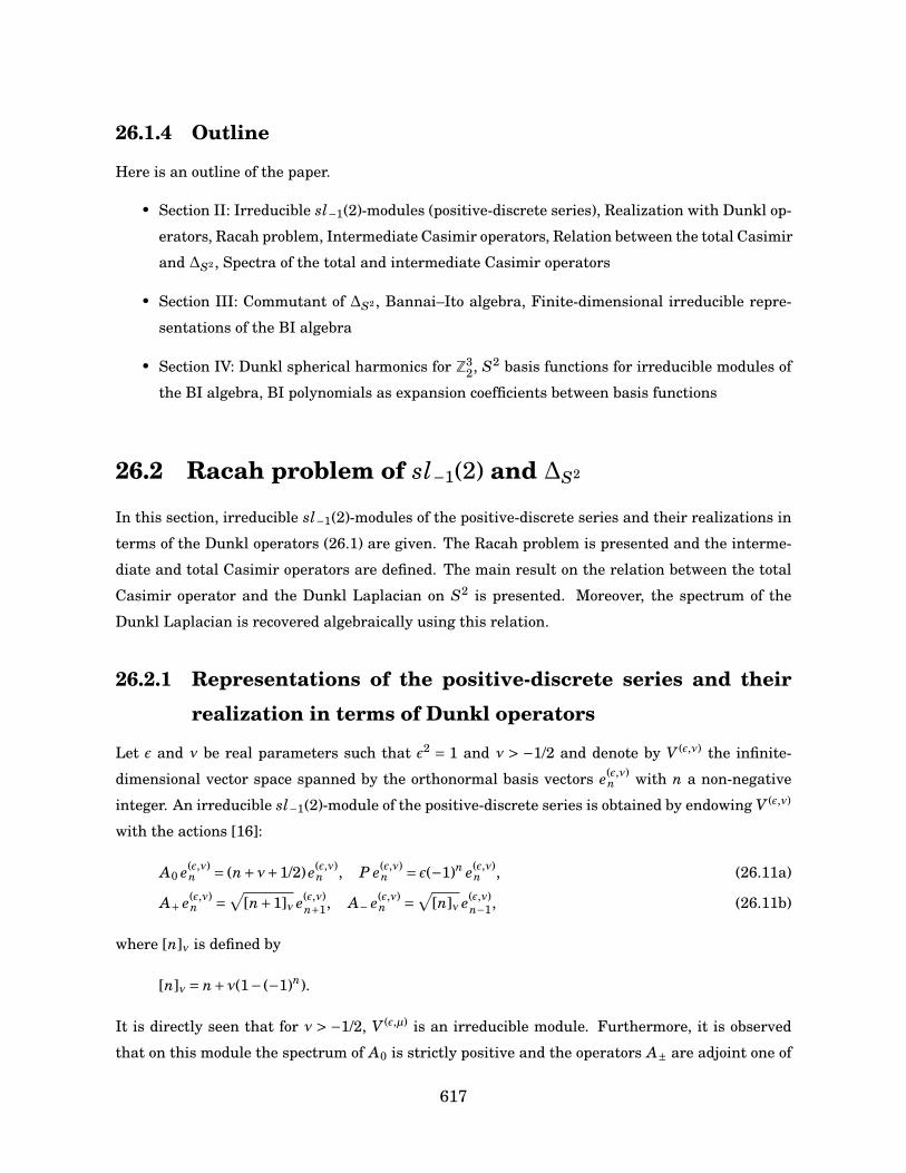
26.1.4 Outline
Here is an outline of the paper.
• Section II: Irreducible sl−1(2)-modules (positive-discrete series), Realization with Dunkl op-
erators, Racah problem, Intermediate Casimir operators, Relation between the total Casimir
and ∆S2 , Spectra of the total and intermediate Casimir operators
• Section III: Commutant of ∆S2 , Bannai–Ito algebra, Finite-dimensional irreducible repre-
sentations of the BI algebra
• Section IV: Dunkl spherical harmonics for Z32, S2 basis functions for irreducible modules of
the BI algebra, BI polynomials as expansion coefficients between basis functions
26.2 Racah problem of sl−1(2) and ∆S2
In this section, irreducible sl−1(2)-modules of the positive-discrete series and their realizations in
terms of the Dunkl operators (26.1) are given. The Racah problem is presented and the interme-
diate and total Casimir operators are defined. The main result on the relation between the total
Casimir operator and the Dunkl Laplacian on S2 is presented. Moreover, the spectrum of the
Dunkl Laplacian is recovered algebraically using this relation.
26.2.1 Representations of the positive-discrete series and their
realization in terms of Dunkl operators
Let ε and ν be real parameters such that ε2 = 1 and ν > −1/2 and denote by V (ε,ν) the infinite-
dimensional vector space spanned by the orthonormal basis vectors e(ε,ν)n with n a non-negative
integer. An irreducible sl−1(2)-module of the positive-discrete series is obtained by endowing V (ε,ν)
with the actions [16]:
A0 e(ε,ν)n = (n+ν+1/2) e(ε,ν)
n , P e(ε,ν)n = ε(−1)n e(ε,ν)
n , (26.11a)
A+ e(ε,ν)n =
√[n+1]ν e(ε,ν)
n+1, A− e(ε,ν)n =
√[n]ν e(ε,ν)
n−1, (26.11b)
where [n]ν is defined by
[n]ν = n+ν(1− (−1)n).
It is directly seen that for ν > −1/2, V (ε,µ) is an irreducible module. Furthermore, it is observed
that on this module the spectrum of A0 is strictly positive and the operators A± are adjoint one of
617
the other. As expected from Schur’s lemma, the Casimir operator (26.6) of sl−1(2) acts a multiple
of the identity on V (ε,ν):
C e(ε,ν)n =−εν e(ε,ν)
n . (26.12)
The sl−1(2)-module V (ε,ν) can be realized using Dunkl operators. Indeed, for each variable xi,
i = 1,2,3, one can check that the operators
A(i)0 =−1
2D2
i +12
x2i , A(i)
± = 1p2
(xi ∓Di), P(i) = Ri, (26.13)
where Di and Ri are as in (26.1), satisfy the defining relations (26.5) of sl−1(2). The Casimir
operator C(i) becomes
C(i) = A(i)+ A(i)
− P(i) − A(i)0 P(i) +P(i)/2=−µi, (26.14)
and hence the operators (26.13) for i = 1,2,3 realize the irreducible module V (ε,ν) with ε = εi = 1
and ν = µi. The orthonormal basis vectors e(εi ,νi)n (xi) in this realization are expressed in terms of
the generalized Hermite polynomials (see for example [7, 14]) and the space V (εi ,νi) with εi = 1
and νi = µi is the L2 space of square integrable functions of argument xi with respect to the
orthogonality measure of the generalized Hermite polynomials [14]; we shall denote it by L2µi
.
26.2.2 The Racah problem, Casimir operators and ∆S2
The Racah problem for sl−1(2)-modules of the positive-discrete series arises when the decompo-
sition in irreducible components of the module V = V (ε1,ν1) ⊗V (ε2,ν2) ⊗V (ε3,ν3) is considered. The
action of the sl−1(2) generators on V is prescribed by the coproduct structure (26.7) and one has
for v ∈V
A0v = (1⊗∆)∆(A0)v, Pv = (1⊗∆)∆(P)v, A±v = (1⊗∆)∆(A±)v. (26.15)
Note that (1⊗∆)∆= (∆⊗1)∆ since ∆ is coassociative. In the realization (26.13), the module V (with
εi = 1 and νi = µi) involves functions of the three independent variables x1, x2, x3. The operators
satisfying the sl−1(2) relations and acting on functions f (x1, x2, x3) in L2µ1
⊗L2µ2
⊗L2µ3
are obtained
from (26.13) and (26.15):
A0 = A(1)0 + A(2)
0 + A(3)0 , P = P(1)P(2)P(3),
A± = A(1)± P(2)P(3) + A(2)
± P(3) + A(3)± .
(26.16)
In combining the modules V (εi ,νi), i = 1,2,3, three types of Casimir operators can be distinguished.
The three initial Casimir operators are those attached to each components V (εi ,µi) of V and act as
618
multiplication by −εiνi as per (26.12). In the realization (26.13), these are the C(i) given in (26.14).
The two intermediate Casimir operators are associated to the two equivalent factorizations
V = (V (ε1,ν1) ⊗V (ε2,ν2))⊗V (ε3,ν3) =V (ε1,ν1) ⊗ (V (ε2,ν2) ⊗V (ε3,ν3)), (26.17)
and correspond to the operators
∆(C)⊗1 and 1⊗∆(C), (26.18)
where ∆(C) is obtained from (26.6) and (26.7). In the realization (26.13), these shall be denoted
C(i j) with (i j)= (12), (23) and are given by
C(i j) = (A(i)+ P(i) + A( j)
+ P( j))(A(i)− P(i) + A( j)
− P( j))
− (A(i)0 + A( j)
0 )P(i)P( j) +P(i)P( j).(26.19)
The total Casimir operator is connected to the whole module V and is of the form (1⊗∆)∆(C). In
the realization (26.13), the total Casimir is denoted C and reads
C = A+ A−P − A0P + P/2. (26.20)
with A0, A± and P given by (26.16). Note that C does not act as a multiple of the identity on V
since in general V is not irreducible.
Remark 13. By construction, the total Casimir operator C commutes with both the initial and in-
termediate Casimir operators. Moreover, it is obvious that the two intermediate Casimir operators
commute with the initial Casimir operators, but do not commute amongst themselves.
We now relate the total Casimir operator C to the Dunkl Laplacian operator ∆S2 on the 2-
sphere.
Proposition 7. Let Ω be the following element:
Ω= CP, (26.21)
where C and P are respectively given by (26.16) and (26.20) in the realization (26.13). One has
−∆S2 =Ω2 +Ω− (µ1 +µ2 +µ3)(µ1 +µ2 +µ3 +1). (26.22)
Proof. The relation is obtained by expanding the total Casimir operator (26.20) using (26.13) and
by writing the resulting operator in the coordinates (26.3).
619
The fact that Ω is a purely angular operator can be understood algebraically as follows. Con-
sider the element X defined by
X = 1p2
(A++ A−
).
It is directly checked that X anticommutes with Ω, that is Ω, X = 0. It thus follows that X2
commutes with Ω. Using the expressions (26.16) for the operators A± in the realization (26.13), it
is easily seen that
X2 = x21 + x2
2 + x23.
Hence Ω commutes with the “radius” operator, which means that it can only be an angular opera-
tor.
26.2.3 Spectrum of ∆S2 from the Racah problem
The relation (26.22) can be exploited to algebraically derive the spectrum of ∆S2 from that of Ω
using the eigenvalues of the intermediate Casimir operators. In view of (26.18), these eigenvalues
can be found from those of ∆(C) on V (εi ,νi) ⊗V (ε j ,ν j) (see also [10, 9, 16] where this problem was
considered). Upon examining the action of ∆(A0) on the direct product basis, one obtains using
(26.11) the following direct sum decomposition of V (εi ,νi) ⊗V (ε j ,ν j) as a vector space:
V (εi ,νi) ⊗V (ε j ,ν j) =∞⊕
n=0Un,
where Un are the (n+1)-dimensional eigenspaces of ∆(A0) with eigenvalue n+νi +ν j +1. Since
∆(C) commutes with ∆(A0), the action of ∆(C) stabilizes Un.
Lemma 14. The eigenvalues λI of ∆(C) on Un are given by
λI (k)= (−1)k+1εiε j(k+νi +ν j +1/2), k = 0, . . .n.
Proof. By induction on n. The n = 0 case is verified by acting with ∆(C) on the single basis vector
e(εi ,νi)0 ⊗e(ε j ,ν j)
0 of U0. Suppose that the result holds at level n−1. Using the fact that ∆(C) and ∆(A+)
commute and the induction hypothesis, one obtains from the action of ∆(A+) on Un−1 eigenvectors
of ∆(C) in Un with eigenvalues λI (k) for k = 0, . . . ,n−1. Let v ∈Un be such that ∆(A−)v = 0. Such
a vector can explicitly be constructed in the direct product basis by solving the corresponding two-
term recurrence relation. It is verified that v is an eigenvector of ∆(P) with eigenvalue (−1)nεiε j
and of ∆(C) with eigenvalue λI (n).
620
As a direct corollary one has the following decomposition of the tensor product module in
irreducible components:
V (εi ,νi) ⊗V (ε j ,ν j) =⊕k
V (εi j(k),νi j(k)), (26.23)
with
εi j(k)= (−1)kεiε j, νi j(k)= k+νi +ν j +1/2, k ∈N. (26.24)
The eigenvalues of the total Casimir operator (1⊗∆)∆(C) on V are obtained by using twice the
decomposition (26.23) and Lemma 1 on (26.17). It is readily seen performing these decompositions
on the LHS of (26.17) that the eigenvalues λT of the total Casimir operator are given by
λT = (−1)k+1ε12(`)ε3(k+ν12(`)+ν3 +1/2), k,` ∈N. (26.25)
A similar formula involving ε23 and ν23 is obtained by considering instead the RHS of (26.17).
Upon using (26.24), the eigenvalues λT can be cast in the form
λT (N)=−ε(N)ν(N), (26.26)
with N a non-negative integer and
ε(N)= (−1)Nε1ε2ε3, ν(N)= (N +ν1 +ν2 +ν3 +1). (26.27)
The formula (26.26) and (26.27) indicate which irreducible modules appear in the decomposition
of V . The multiplicity of V (ε(N),ν(N)) in this decomposition is N+1 since for a given value of N there
are N +1 possible eigenvalues of the intermediate Casimir operators; the decomposition formula
for V is thus
V =∞⊕
N=0mNV (ε(N),ν(N)), (26.28)
where mN = N +1 and where ε(N), ν(N) are given by (26.27).
Returning to the realization (26.16) of the module V with εi = 1 and νi = µi, the eigenvalues
of Ω = CP are readily obtained. Recalling (26.12), it follows from (26.26) and (26.27) that the
eigenvalues ωN of Ω are
ωN =−(N +µ1 +µ2 +µ3 +1), (26.29)
where N is a non-negative integer. The relation (26.22) then leads to the following.
Proposition 8. The eigenvalues δ of the Dunkl Laplacian ∆S2 on the 2-sphere are indexed by the
non-negative integer N and have the expression
δN =−N(N +2µ1 +2µ2 +2µ3 +1). (26.30)
621
Proof. By proposition 1 and the above considerations.
The eigenvalues of proposition 2 are in accordance with those obtained in [6]. It is seen that
upon specializing (26.30) to µ1 = µ2 = µ3 = 0, one recovers the spectrum of the standard Laplacian
on the 2-sphere. It is worth mentioning that the formula (26.30) does not provide information on
the degeneracy of the eigenvalues. This question will be discussed in the following.
26.3 Commutant of ∆S2 and the Bannai–Ito algebra
In this section, the operators commuting with the Dunkl Laplacian on the 2-sphere are exhib-
ited and are shown to generate a central extension of the Bannai–Ito algebra. The eigensub-
spaces corresponding to the simultaneous diagonalization of ∆S2 and Ω are seen to support finite-
dimensional irreducible representations of the BI algebra and the matrix elements of these repre-
sentations are constructed.
26.3.1 Commutant of ∆S2 and symmetry algebra
The operators that commute with the Dunkl Laplacian ∆S2 on the 2-sphere, referred to as the
symmetries of ∆S2 , can be obtained from the relation (26.22) and the framework provided by the
Racah problem of sl−1(2). By construction, the intermediate Casimir operators (26.19) commute
with the total Casimir (26.20) and with the involution P. As a consequence of (26.22), one thus
has
[∆S2 ,C(12)]= [∆S2 ,C(23)]= 0.
Let K1, K3 be the following operators:
K1 =−C(23), K3 =−C(12), (26.31)
which obviously commute with the Dunkl Laplacian on S2. Upon using (26.13) and (26.19), the
symmetries K1, K3 are seen to have the expressions
K1 = (x2D3 − x3D2)R2 +µ2R3 +µ3R2 + (1/2)R2R3, (26.32a)
K3 = (x1D2 − x2D1)R1 +µ1R2 +µ2R1 + (1/2)R1R2, (26.32b)
where Di and Ri are given by (26.1). Consider the operator K2 defined by
K2 = (x1D3 − x3D1)R1R2 +µ1R3 +µ3R1 + (1/2)R1R3. (26.32c)
It is verified by an explicit calculation that K2 is also a symmetry of the Dunkl-Laplacian ∆S2 , i.e.
[∆S2 ,K2]= 0.
622

Remark 15. Note that K2 does not correspond to an intermediate Casimir operator since it has a
non-trivial action on all three variables x1, x2, x3.
The three operators K i, i = 1,2,3, and the operator Ω given by (26.21) are not independent
from one another. As a matter of fact, one has
Ω=−K1R2R3 −K2R1R3 −K3R1R2 +µ1R1 +µ2R2 +µ3R3 +1/2.
We now give the symmetry algebra generated by the operators commuting with the Dunkl-Laplace
operator ∆S2 on the 2-sphere.
Proposition 9. Let ∆S2 be the Dunkl Laplacian (26.4) on the 2-sphere and let C and K i, i = 1,2,3
be given by (26.20) and (26.32), respectively. One has
[∆S2 ,K i]= [∆S2 , C]= 0.
and the symmetry algebra of ∆S2 is
K1,K2= K3 −2µ3C+2µ1µ2, (26.33a)
K2,K3= K1 −2µ1C+2µ2µ3, (26.33b)
K3,K1= K2 −2µ2C+2µ1µ3. (26.33c)
Proof. By an explicit calculation using (26.4) and (26.32).
The algebra (26.33) corresponds to a central extension of the Bannai–Ito algebra (26.8) by the
total Casimir operator C. Since C (and Ω) commutes with ∆S2 , there is a basis in which they are
both diagonal. From (26.27) and (26.29), it follows that the eigenvalues of C are of the form −εµwith
ε= (−1)N , µ= (N +µ1 +µ2 +µ3 +1). (26.34)
For a given N, the ∆S2-eigenspaces arising under the joint diagonalization of ∆S2 and C (or Ω) are
(N+1)-dimensional as per the decomposition (26.28) of the tensor product module V in irreducible
components. Hence the eigenvalues δN of ∆S2 given by (26.30) are at least (N+1)-fold degenerate.
It can be seen that this degeneracy is in fact higher. Indeed, ∆S2 commutes with every reflection
operator Ri, but C (and Ω) only commute with their product R1R2R3. Consequently one can
obtain eigenfunctions of ∆S2 with eigenvalue δN that are not eigenfunctions of C by applying any
reflection Ri on a given eigenfunction of C. It is known [6] that the eigenspaces corresponding to
the eigenvalue δN are in fact (2N +1)-fold degenerate, as shall be seen in Section 4.
Notwithstanding the degeneracy question, it follows from Proposition 3 and (26.34) that the
eigensubspaces of the Laplace-Dunkl operator corresponding to the simultaneous diagonalization
623
of ∆S2 and C support an (N +1)-dimensional module of the Bannai–Ito algebra (26.8) with struc-
ture constants taking the values
α1 = 2(µ1µ+µ2µ3), α2 = 2(µ1µ3 +µ2µ), α3 = 2(µ1µ2 +µ3µ), (26.35)
where µ= (−1)N (N +µ1 +µ2 +µ3 +1). The Casimir operator K2 = K21 +K2
2 +K23 of the Bannai–Ito
algebra can be expressed in terms of C as follows:
K2 = C2 +µ21 +µ2
2 +µ23 −1/4,
and hence using (26.34) one has
K2 =µ21 +µ2
2 +µ23 +µ2 −1/4. (26.36)
The realization (26.35), (26.36) of the Bannai–Ito algebra corresponds to the one arising in the
Racah problem for sl−1(2) studied in [10]. We shall now obtain the matrix elements of the genera-
tors in this realization.
26.3.2 Irreducible modules of the Bannai–Ito algebra
We begin by examining the representations of (26.8) with structure constants (26.35) in the eigen-
basis ψkNk=0 of K3. Using the result of Lemma 1 and (26.31), it follows that
K3ψk =ωkψk, ωk = (−1)k(k+µ1 +µ2 +1/2), (26.37)
We define the action of K1 by
K1ψk =∑s
Zs,kψs. (26.38)
From the second relation of (26.8) one finds∑s
Zs,k[(ωk +ωs)2 −1
]ψs = [α1 +2ωkα2]ψk.
When s = k, one immediately obtains
Zk,k ≡Vk =α1 +2ωkα2
4ω2k −1
. (26.39)
When s 6= k, one of the following conditions must hold
(ωk +ωs)2 −1= 0, or Zs,k = 0.
In view of the formula (26.37) for the eigenvalues ωk, it is directly seen that only Zk+1,k, Zk,k and
Zk−1,k can be non-vanishing. Thus one can take
K1ψk =Uk+1ψk+1 +Vkψk +Ukψk−1, (26.40)
624
where Vk is given by (26.39) and where Uk remains to be determined. It follows from (26.8) and
(26.40) that K2 has the action
K2ψk = (−1)k+1Uk+1 +Wkψk + (−1)kUkψk−1, (26.41)
where Wk = 2ωkVk −α2. Upon using the actions (26.40), (26.41) in the first relation of (26.8) and
comparing the terms in ψk, one obtains the recurrence relation for U2k
2(−1)k+1U2
k+1 +WkVk + (−1)kU2k
=ωk +α3. (26.42)
Acting on ψk with (26.36) and using the actions (26.40), (26.41), one finds
ω2
k +W2k +V 2
k +2U2k +2U2
k+1=µ2
1 +µ22 +µ2
3 +µ2 −1/4. (26.43)
The equations (26.42), (26.43) can be used to solve for U2k by eliminating U2
k+1. Straightforward
calculations then lead to the following result.
Proposition 10. Let W be the (N +1)-dimensional vector space spanned by the basis vectors ψk,
k = 0, . . . , N, and let
µ= (−1)N (N +1+µ1 +µ2 +µ3). (26.44)
An irreducible module for the Bannai–Ito algebra (26.8) with structure constants (26.35) is obtained
by endowing W with the actions
K3ψk =ωkψk, (26.45a)
K2ψk = (−1)k+1Uk+1ψk+1 + (2ωkVk −α2)ψk + (−1)kUkψk−1, (26.45b)
K1ψk =Uk+1ψk+1 +Vkψk +Ukψk−1, (26.45c)
where ωk = (−1)k(k+µ1 +µ2 +1/2), Vk =µ2 +µ3 +1/2−Bk −Dk and where Uk =√
Bk−1Dk with
Bk =
(k+2µ2+1)(k+µ1+µ2+µ3−µ+1)
2(k+µ1+µ2+1) , k is even,(k+2µ1+2µ2+1)(k+µ1+µ2+µ3+µ+1)
2(k+µ1+µ2+1) , k is odd,
Dk =
−k(k+µ1+µ2−µ3−µ)
2(k+µ1+µ2) , k is even,−(k+2µ1)(k+µ1+µ2−µ3+µ)
2(k+µ1+µ2) , k is odd.
Proof. One verifies directly that with (26.45) the defining relations (26.8), (26.35) are satisfied.
The irreducibility follows from the fact that Uk 6= 0 for µi >−1/2.
In view of Proposition 4, it is natural to wonder what the representation matrix elements look
like in other bases, say the eigenbases of either K1 or K2. These elements are easily obtained
625
from the Z3 symmetry of the realization (26.35), (26.36). Indeed, it is verified that the algebra
(26.8) with (26.35), (26.36) is left invariant by any cyclic transformation of both K1,K2,K3 and
µ1,µ2,µ3. As a consequence, the representation matrix elements in the K1 or K2 eigenbasis can
be obtained directly from Proposition 4 by applying the permutation π= (123) or π= (123)2 on the
generators K i and the parameters µi.
26.4 S2 basis functions for irreducible
Bannai–Ito modules
In this section, a family of orthonormal functions on S2 that realize bases for the Bannai–Ito
modules of Proposition 4 are constructed. It is shown that the Bannai–Ito polynomials arise as
the overlap coefficients between two such bases separated in different spherical coordinates.
26.4.1 Harmonics for ∆S2
It is useful to give here the Dunkl spherical harmonics YN (θ,φ) which are the regular solutions to
the eigenvalue equation
∆S2YN (θ,φ)= δNYN (θ,φ), δN =−N(N +2µ1 +2µ2 +2µ3 +1), (26.46)
where ∆S2 is given by (26.4). The solutions to (26.46) are well known and are given explicitly in
[6] in terms of the generalized Gegenbauer polynomials. We give their expressions here in terms
of Jacobi polynomials. In spherical coordinates (26.3), the solutions to (26.46) read
Y (e1,e2,e3)n;N (θ,φ)= η(e1,e2,e3)
n;N cose3 θsinn θ cose1 φsine2 φ
×P(n+µ1+µ2,µ3+e3−1/2)(N−n−e3)/2 (cos2θ) P(µ2+e2−1/2,µ1+e1−1/2)
(n−e1−e2)/2 (cos2φ), (26.47)
where e i ∈ 0,1, n is a non-negative integer, η(e1,e2,e3)N,n is a normalization factor and P(α,β)
n (x) are
the standard Jacobi polynomials [12]. The harmonics (26.47) satisfy
Ri Y (e1,e2,e3)n;N (θ,φ)= (1−2e i)Y
(e1,e2,e3)n;N (θ,φ).
In (26.47), it is understood that half-integer (or negative) indices in P(α,β)n (x) do not provide admis-
sible solutions. Recording the admissible values of n and e i for a given N, one finds that there are
2N +1 solutions and
R1R2R3Y (e1,e2,e3)n;N (θ,φ)= (−1)NY (e1,e2,e3)
n;N (θ,φ).
626
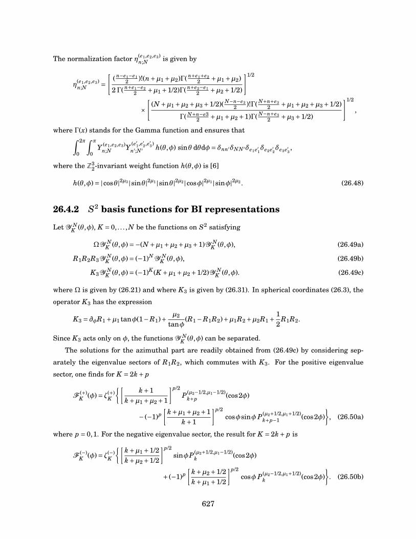
The normalization factor η(e1,e2,e3)n;N is given by
η(e1,e2,e3)n;N =
[( n−e1−e1
2 )!(n+µ1 +µ2)Γ( n+e1+e22 +µ1 +µ2)
2Γ( n+e1−e22 +µ1 +1/2)Γ( n+e2−e1
2 +µ2 +1/2)
]1/2
×[
(N +µ1 +µ2 +µ3 +1/2)( N−n−e32 )!Γ( N+n+e3
2 +µ1 +µ2 +µ3 +1/2)
Γ( N+n−e32 +µ1 +µ2 +1)Γ( N−n+e3
2 +µ3 +1/2)
]1/2
,
where Γ(x) stands for the Gamma function and ensures that∫ 2π
0
∫ π
0Y (e1,e2,e3)
n;N Y (e′1,e′2,e′3)n′;N ′ h(θ,φ) sinθ dθdφ= δnn′δNN ′δe1e′1δe2e′2δe3e′3 ,
where the Z32-invariant weight function h(θ,φ) is [6]
h(θ,φ)= |cosθ|2µ3 |sinθ|2µ1 |sinθ|2µ2 |cosφ|2µ1 |sinφ|2µ2 . (26.48)
26.4.2 S2 basis functions for BI representations
Let Y NK (θ,φ), K = 0, . . . , N be the functions on S2 satisfying
ΩY NK (θ,φ)=−(N +µ1 +µ2 +µ3 +1)Y N
K (θ,φ), (26.49a)
R1R2R3 Y NK (θ,φ)= (−1)N Y N
K (θ,φ), (26.49b)
K3 Y NK (θ,φ)= (−1)K (K +µ1 +µ2 +1/2)Y N
K (θ,φ). (26.49c)
where Ω is given by (26.21) and where K3 is given by (26.31). In spherical coordinates (26.3), the
operator K3 has the expression
K3 = ∂φR1 +µ1 tanφ(1−R1)+ µ2
tanφ(R1 −R1R2)+µ1R2 +µ2R1 + 1
2R1R2.
Since K3 acts only on φ, the functions Y NK (θ,φ) can be separated.
The solutions for the azimuthal part are readily obtained from (26.49c) by considering sep-
arately the eigenvalue sectors of R1R2, which commutes with K3. For the positive eigenvalue
sector, one finds for K = 2k+ p
F (+)K (φ)= ζ(+)
K
[k+1
k+µ1 +µ2 +1
]p/2P(µ2−1/2,µ1−1/2)
k+p (cos2φ)
− (−1)p[
k+µ1 +µ2 +1k+1
]p/2cosφsinφ P(µ2+1/2,µ1+1/2)
k+p−1 (cos2φ)
, (26.50a)
where p = 0,1. For the negative eigenvalue sector, the result for K = 2k+ p is
F (−)K (φ)= ζ(−)
K
[k+µ1 +1/2k+µ2 +1/2
]p/2sinφP(µ2+1/2,µ1−1/2)
k (cos2φ)
+ (−1)p[
k+µ2 +1/2k+µ1 +1/2
]p/2cosφ P(µ2−1/2,µ1+1/2)
k (cos2φ)
. (26.50b)
627
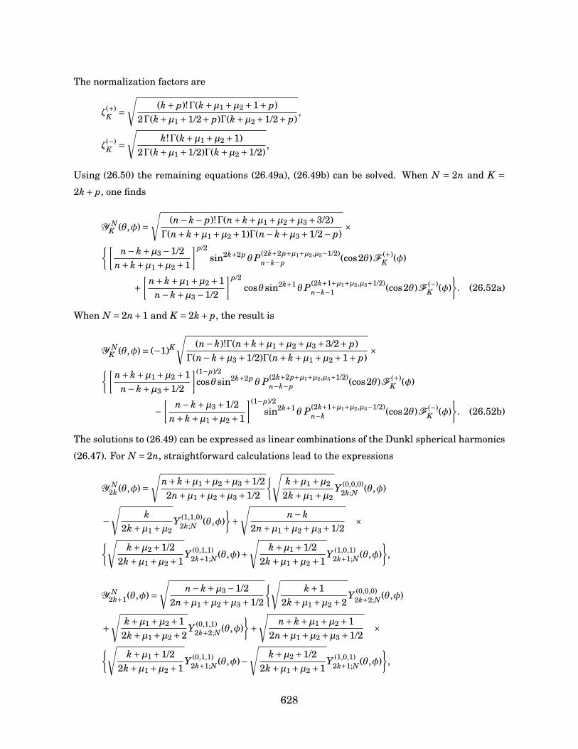
The normalization factors are
ζ(+)K =
√(k+ p)!Γ(k+µ1 +µ2 +1+ p)
2Γ(k+µ1 +1/2+ p)Γ(k+µ2 +1/2+ p),
ζ(−)K =
√k!Γ(k+µ1 +µ2 +1)
2Γ(k+µ1 +1/2)Γ(k+µ2 +1/2),
Using (26.50) the remaining equations (26.49a), (26.49b) can be solved. When N = 2n and K =2k+ p, one finds
Y NK (θ,φ)=
√(n−k− p)!Γ(n+k+µ1 +µ2 +µ3 +3/2)
Γ(n+k+µ1 +µ2 +1)Γ(n−k+µ3 +1/2− p)×[
n−k+µ3 −1/2n+k+µ1 +µ2 +1
]p/2sin2k+2p θP(2k+2p+µ1+µ2,µ3−1/2)
n−k−p (cos2θ)F (+)K (φ)
+[
n+k+µ1 +µ2 +1n−k+µ3 −1/2
]p/2cosθsin2k+1θP(2k+1+µ1+µ2,µ3+1/2)
n−k−1 (cos2θ)F (−)K (φ)
. (26.52a)
When N = 2n+1 and K = 2k+ p, the result is
Y NK (θ,φ)= (−1)K
√(n−k)!Γ(n+k+µ1 +µ2 +µ3 +3/2+ p)
Γ(n−k+µ3 +1/2)Γ(n+k+µ1 +µ2 +1+ p)×[
n+k+µ1 +µ2 +1n−k+µ3 +1/2
](1−p)/2cosθsin2k+2p θ P(2k+2p+µ1+µ2,µ3+1/2)
n−k−p (cos2θ)F (+)K (φ)
−[
n−k+µ3 +1/2n+k+µ1 +µ2 +1
](1−p)/2sin2k+1θ P(2k+1+µ1+µ2,µ3−1/2)
n−k (cos2θ)F (−)K (φ)
. (26.52b)
The solutions to (26.49) can be expressed as linear combinations of the Dunkl spherical harmonics
(26.47). For N = 2n, straightforward calculations lead to the expressions
Y N2k (θ,φ)=
√n+k+µ1 +µ2 +µ3 +1/22n+µ1 +µ2 +µ3 +1/2
√k+µ1 +µ2
2k+µ1 +µ2Y (0,0,0)
2k;N (θ,φ)
−√
k2k+µ1 +µ2
Y (1,1,0)2k;N (θ,φ)
+
√n−k
2n+µ1 +µ2 +µ3 +1/2×
√k+µ2 +1/2
2k+µ1 +µ2 +1Y (0,1,1)
2k+1;N (θ,φ)+√
k+µ1 +1/22k+µ1 +µ2 +1
Y (1,0,1)2k+1;N (θ,φ)
,
Y N2k+1(θ,φ)=
√n−k+µ3 −1/2
2n+µ1 +µ2 +µ3 +1/2
√k+1
2k+µ1 +µ2 +2Y (0,0,0)
2k+2;N (θ,φ)
+√
k+µ1 +µ2 +12k+µ1 +µ2 +2
Y (0,1,1)2k+2;N (θ,φ)
+
√n+k+µ1 +µ2 +1
2n+µ1 +µ2 +µ3 +1/2×
√k+µ1 +1/2
2k+µ1 +µ2 +1Y (0,1,1)
2k+1;N (θ,φ)−√
k+µ2 +1/22k+µ1 +µ2 +1
Y (1,0,1)2k+1;N (θ,φ)
,
628
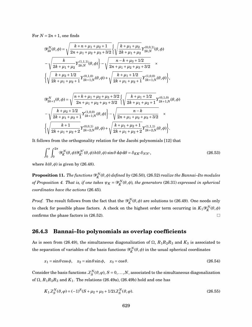
For N = 2n+1, one finds
Y N2k (θ,φ)=
√k+n+µ1 +µ2 +1
2n+µ1 +µ2 +µ3 +3/2
√k+µ1 +µ2
2k+µ1 +µ2Y (0,0,1)
2k;N (θ,φ)
−√
k2k+µ1 +µ2
Y (1,1,1)2k;N (θ,φ)
−
√n−k+µ3 +1/2
2n+µ1 +µ2 +µ3 +3/2×
√k+µ2 +1/2
2k+µ1 +µ2 +1Y (0,1,0)
2k+1;N (θ,φ)+√
k+µ1 +1/22k+µ1 +µ2 +1
Y (1,0,0)2k+1;N (θ,φ)
,
Y N2k+1(θ,φ)=
√n+k+µ1 +µ2 +µ3 +3/22n+µ1 +µ2 +µ3 +3/2
√k+µ1 +1/2
2k+µ1 +µ2 +1Y (0,1,0)
2k+1;N (θ,φ)
−√
k+µ2 +1/22k+µ1 +µ2 +1
Y (1,0,0)2k+1;N (θ,φ)
−
√n−k
2n+µ1 +µ2 +µ3 +3/2×
√k+1
2k+µ1 +µ2 +2Y (0,0,1)
2k+2;N (θ,φ)+√
k+µ1 +µ2 +12k+µ1 +µ2 +2
Y (1,1,1)2k+2;N (θ,φ)
.
It follows from the orthogonality relation for the Jacobi polynomials [12] that∫ π
0
∫ 2π
0Y N
K (θ,φ)Y N ′K ′ (θ,φ)h(θ,φ) sinθ dφdθ = δKK ′δNN ′ , (26.53)
where h(θ,φ) is given by (26.48).
Proposition 11. The functions Y NK (θ,φ) defined by (26.50), (26.52) realize the Bannai–Ito modules
of Proposition 4. That is, if one takes ψK = Y NK (θ,φ), the generators (26.31) expressed in spherical
coordinates have the actions (26.45).
Proof. The result follows from the fact that the Y NK (θ,φ) are solutions to (26.49). One needs only
to check for possible phase factors. A check on the highest order term occurring in K1Y NK (θ,φ)
confirms the phase factors in (26.52).
26.4.3 Bannai–Ito polynomials as overlap coefficients
As is seen from (26.49), the simultaneous diagonalization of Ω, R1R2R3 and K3 is associated to
the separation of variables of the basis functions Y NK (θ,φ) in the usual spherical coordinates
x1 = sinθ cosφ, x2 = sinθsinφ, x3 = cosθ. (26.54)
Consider the basis functions Z NS (ϑ,ϕ), S = 0, . . . , N, associated to the simultaneous diagonalization
of Ω, R1R2R3 and K1. The relations (26.49a), (26.49b) hold and one has
K1Z NS (ϑ,ϕ)= (−1)S(S+µ2 +µ3 +1/2)Z N
S (ϑ,ϕ). (26.55)
629

The functions Z NS (ϑ,ϕ) separate in the alternative spherical coordinates
x1 = cosϑ, x2 = sinϑcosϕ, x3 = sinϑsinϕ, (26.56)
as can be seen from the expression of K1 obtained using (26.56). Writing Ω in the coordinates
(26.56) and comparing the expression with the one obtained using the coordinates (26.54), it is
seen that the basis functions Z NS (ϑ,ϕ) have the expression
Z NS (ϑ,ϕ)=
πY NS (π−ϑ,ϕ), N is even,
πY NS (ϑ,ϕ), N is odd,
where π= (123) is the permutation applied to the parameters (µ1,µ2,µ3). Since Y NK (θ,φ)N
K=0 and
Z NS (ϑ,ϕ)N
S=0 form orthonormal bases for the same space, they are related (at a given point) by a
unitary transformation. One hence writes
Z NS (ϑ,ϕ)=
N∑K=0
Rµ1,µ2,µ3S,K ;N Y N
K (θ,φ). (26.57)
Since the coefficients Rµ1,µ2,µ3S,K ;N are real, their unitarity implies
N∑S=0
Rµ1µ2µ3S,K ;N Rµ1µ2µ3
S,K ′;N = δKK ′ ,N∑
K=0Rµ1µ2µ3
S,K ;N Rµ1µ2µ3S′,K ;N = δSS′ , (26.58)
These transition coefficients can be expressed in terms of the Bannai–Ito polynomials (26.9) as
follows. Acting with K1 on both sides of (26.57), using (26.55) and Proposition 5 and further-
more defining Rµ1,µ2,µ3S,K ;N = 2K [wS;N ]1/2BK (xS) such that B0(xS) = 1, it seen that BK (xS) satisfy the
three-term recurrence relation (26.9) of the Bannai–Ito polynomials BK (xS;ρ1,ρ2, r1, r2) with pa-
rameters
ρ1 = µ2 +µ3
2, ρ2 = µ1 +µ
2, r1 = µ3 −µ2
2, r2 = µ−µ1
2. (26.59)
with µ given by (26.44) and where the variable xS is given by
xS = 12
[(−1)S(S+µ2 +µ3 +1/2)−1/2
]. (26.60)
The coefficients Rµ1µ2µ3S,K ;N coincide with the Racah coefficients of sl−1(2) [10]. Combining (26.58) with
the orthogonality relation of the BI polynomial [17], one finds
Rµ1µ2µ3S,K ;N =
√wS;N
u1u2 · · ·uKBK (xS;ρ1,ρ2, r1, r2). (26.61)
with (26.59), (26.60), where un = An−1Cn with An, Cn as in (26.10), and where wS;N is of the form
wS;N = 1hN
(−1)ν(ρ1 − r1 +1/2;ρ1 − r2 +1/2)`+ν(ρ1 +ρ2 +1;2ρ1 +1)`(ρ1 + r1 +1/2;ρ1 + r2 +1/2)`+ν(1;ρ1 −ρ2 +1)`
,
630

with S = 2`+ν, ν= 0,1 and
(a1;a2; . . . ;ak)n = (a1)n(a2)n · · · (ak)n, (26.62)
where (a)n = a(a+1) · · · (a+n−1). The normalization factor hN is given by
hN =
(2ρ1+1;r1−ρ2+1/2)N/2
(ρ1−ρ2+1;ρ1+r1+1/2)N/2, N even,
(2ρ1+1;r1+r2)(N+1)/2(ρ1+r1+1/2;ρ1+r2+1/2)(N+1)/2
, N odd.
Using the orthogonality relation (26.53) satisfied by the basis functions Y NK (θ,φ) on the decompo-
sition formula (26.57), one finds that
Rµ1µ2µ3S,K ;N =
∫ π
0
∫ 2π
0Y N
K (θ,φ)Z NS (ϑ,ϕ)h(θ,φ) sinθdφdθ,
which in light of (26.61) gives an integral formula for the Bannai–Ito polynomials.
26.5 Conclusion
We have established in this paper the algebraic basis for the harmonic analysis on S2 associated to
a Z32 Dunkl Laplacian ∆2
S. The commutant of ∆S2 was determined in the framework of the Racah
problem for sl−1(2) and identified with a central extension of the Bannai–Ito algebra. Two bases
for the unitary irreducible representations of this algebra on L2(S2) were explicitly constructed
in terms of the Dunkl spherical harmonics with the Bannai–Ito orthogonal polynomials arising in
their overlaps.
Since the Dunkl operators and Laplacian can be defined for an arbitrary number of variables,
it would be natural to look for the extension of the results presented here to spheres in higher
dimensions. It would be also of interest to examine the situation on hyperboloids. We plan to
pursue the study of these questions in the future.
References[1] E. Bannai and T. Ito. Algebraic Combinatorics I: Association Schemes. Benjamin/Cummings,
1984.
[2] C. Daskaloyannis and K. Kanakoglou. Hopf algebraic structure of the parabosonic and
parafermionic algebras and paraparticle generalization of the Jordan-Schwinger map. J.
Math. Phys., 41:652–660, 2000.
[3] H. DeBie, B. Ørsted, P. Somberg, and V. Soucek. Dunkl Operators and a family of realizations
of osp(1|2). Trans. Amer. Math. Soc., 364:3875–3902, 2012.
631

[4] C. F. Dunkl. Reflection Groups and Orthogonal Polynomials on the Sphere. Mathematische
Zeitschrift, 197:33–60, 1988.
[5] C. F. Dunkl. Differential-difference operators associated to reflection groups. Trans. Amer.
Math. Soc., 311:167–183, 1989.
[6] C. F. Dunkl and Y. Xu. Orthogonal Polynomials of Several Variables. Cambridge University
Press, 2001.
[7] V.X. Genest, M.E.H. Ismail, L. Vinet, and A. Zhedanov. The Dunkl oscillator in the plane:
I. Superintegrability, separated wavefunctions and overlap coefficients. J. Phys. A: Math.
Theor., 46:145201, 2013.
[8] V.X. Genest, L. Vinet, and A. Zhedanov. Bispectrality of the Complementary Bannai–Ito
polynomials. SIGMA, 9:18–37, 2013.
[9] V.X. Genest, L. Vinet, and A. Zhedanov. The algebra of dual −1 Hahn polynomials and the
Clebsch-Gordan problem of sl−1(2). J. Math. Phys., 54:023506, 2013.
[10] V.X. Genest, L. Vinet, and A. Zhedanov. The Bannai-Ito polynomials as Racah coefficients of
the sl−1(2) algebra. Proc. Am. Soc., 142:1545–1560, 2014.
[11] P. Graczyk, M. Rösler, M. Yor, and N. Demni, editors. Harmonic and Stochastic Analysis of
Dunkl Processes. Hermann, 2008.
[12] R. Koekoek, P.A. Lesky, and R.F. Swarttouw. Hypergeometric orthogonal polynomials and
their q-analogues. Springer, 1st edition, 2010.
[13] E. Opdam. Lecture notes on Dunkl operators. Technical report, University of Leiden, 1998.
[14] M. Rosenblum. Generalized Hermite polynomials and the Bose-like oscillator calculus. In
Nonselfadjoint Operators and Related Topics, Operator Theory: Advances and Applications.
Springer, 1994.
[15] M. Rösler. Dunkl Operators: Theory and Applications. In Orthogonal Polynomials and Spe-
cial Functions, Lecture Notes in Mathematics Vol. 1817, pages 93–135. Springer, 2003.
[16] S. Tsujimoto, L. Vinet, and A. Zhedanov. From slq(2) to a parabosonic Hopf algebra. SIGMA,
7:93–105, 2011.
[17] S. Tsujimoto, L. Vinet, and A. Zhedanov. Dunkl shift operators and Bannai–Ito polynomials.
Adv. Math., 229:2123–2158, 2012.
632
[18] R. G. Underwood. An Introduction to Hopf algebras. Springer, 2011.
[19] J. F. van Diejen and L. Vinet, editors. Calogero–Moser–Sutherland Models. CRM Series in
Mathematical Physics. Springer, 2000.
[20] N. Ja. Vilenkin and A. U. Klimyk. Representation of Lie Groups and Special Functions.
Kluwer Academic Publishers, 1991.
633

634
Partie V
Polynômes multi-orthogonauxmatriciels
et applications
635

Introduction
Le théorème de Favard [36] stipule que toute famille de polynômes orthogonaux Pn(x)∞n=0 obéit à
une relation de récurrence à trois termes de la forme
xPn(x)= Pn+1(x)+bnPn(x)+ cnPn−1(x),
avec P−1(x) = 0, P0(x) = 1 et où bn et cn sont des coefficients numériques. Réciproquement, il
stipule aussi que toute famille Pn(x)∞n=0 qui obéit à une relation de récurrence à trois termes de
la forme ci-haut forme nécessairement une famille orthogonale.
Les polynômes multi-orthogonaux matriciels sont une généralisation des polynômes orthogo-
naux: ils sont caractérisés par des relations de récurrence d’ordre plus élevé [65]. Par exemple,
supposons que l’on ait affaire à la relation de récurrence
xPn(x)= anPn+2(x)+bnPn+1(x)+ cnPn(x)+dnPn−1(x)+ enPn−2(x),
avec certaines conditions initiales. Le polynôme vectoriel
Qn(x)= (P2n(x),P2n+1(x))>,
obéit alors à la relation de récurrence
x Qn(x)= AnQn+1(x)+BnQn(x)+CnQn−1(x),
où An, Bn et Cn sont maintenant des matrices 2×2. En général, les polynômes multi-orthogonaux
obéissent à de multiples relations d’orthogonalité matricielles.
Dans cette partie de la thèse, on étudie deux nouvelles familles de polynômes vectoriels multi-
orthogonaux qui interviennent dans les éléments de matrices d’exponentielles quadratiques dans
les générateurs de su(2). On utilise ensuite ces résultats dans l’étude des états cohérents et com-
primés de l’oscillateur fini, ce qui mène aussi à la caractérisation d’une famille de polynômes
matriciels multi-orthogonaux.
637

638
Chapitre 27
d-Orthogonal polynomials and su(2)
V. X. Genest, L. Vinet et A. Zhedanov (2012). d-Orthogonal polynomials and su(2). Journal of
Mathematical Analysis and Applications 390 472-487
Abstract. Two families of d-orthogonal polynomials related to su(2) are identified and studied.
The algebraic setting allows for their full characterization (explicit expressions, recurrence rela-
tions, difference equations, generating functions, etc.). In the limit where su(2) contracts to the
Heisenberg-Weyl algebra h1, the polynomials tend to the standard Meixner polynomials and d-
Charlier polynomials, respectively.
27.1 Introduction
We identify in this paper two families of d-orthogonal polynomials that are associated to su(2).
When available, algebraic models for orthogonal polynomials provide a cogent framework for the
characterization of these special functions. They also point to the likelihood of seeing the corre-
sponding polynomials occur in the description of physical systems whose symmetry generators
form the algebra in question.
d-orthogonal polynomials generalize the standard orthogonal polynomials in that they obey
higher recurrence relations. They will be defined below and have been seen to possess various
applications [6, 7, 13]. Recently, two of us have uncovered the connection between d-Charlier
polynomials and the Heisenberg algebra. Here we pursue this exploration of d-orthogonal poly-
nomials related to Lie algebras by considering the case of su(2). Remarkably, two hypergeometric
families of such polynomials will be identified and characterized.
639
27.1.1 d-Orthogonal polynomials
The monic d-orthogonal polynomials Pn(k) of degree n (Pn(k) = kn + . . .) can be defined by the
recurrence relation [10]
Pn+1(k)= kPn(k)−d∑
µ=0an,n−µPn−µ(k), (27.1)
of order d+1 with complex coefficients an,m; the initial conditions are Pn = 0 if n < 0 and P0 = 1.
It is assumed that an,n−d 6= 0 (non-degeneracy condition).
When d = 1, it is known that under the condition cn 6= 0, the polynomials satisfying three-term
recurrence relations
Pn+1(k)= kPn(k)−bnPn(k)− cnPn−1(k),
are orthogonal with respect to a linear functional σ
⟨σ, Pn(k)Pm(k)⟩ = δnm,
defined on the space of all polynomials.
When d > 1, the polynomials Pn(k) obey vector orthogonality relations. This means that there
exists a set of d linear functionals σi for i = 0, . . . , d−1 such that the following relations hold:
⟨σi, PnPm⟩ = 0, if m > dn+ i,
⟨σi, PnPdn+i⟩ 6= 0, if n> 0.
27.1.2 d-Orthogonal polynomials as
generalized hypergeometric functions
Of particular interest are d-orthogonal polynomials that can be expressed in terms of generalized
hypergeometric functions (see for instance [1, 2, 5]). These functions are denoted pFq and are
defined by
pFq
ap
bq;1c
:=∞∑µ=0
(a1)µ · · · (ap)µ(b1)µ · · · (bq)µ
c−µ
µ!,
where (m)0 = 1 and (m)k = (m)(m+1) · · · (m+k−1) stands for the Pochhammer symbol. In the case
where one of the ai ’s is a negative integer, say a1 =−n for n ∈N, the series truncates at µ= n and
we can write
1+sFq
−n, as
bq;1c
=n∑
µ=0
(−n)µ(a1)µ · · · (as)µ(b1)µ · · · (bq)µ
c−µ
µ!. (27.2)
640
If one of the bi ’s is also a negative integer, the corresponding sequence of polynomials is finite.
The classification of d-orthogonal polynomials that have a hypergeometric representation of
the form (27.2) has been studied recently in [3]. The results are as follows.
Let s> 1 and let as= a1, . . . ,as be a set of s polynomials of degree one in the variable k. This
set is called s-separable if there is a polynomial π(y) such that∏s
i=1(ai(k)+ y)= [∏s
i=1 ai(k)]+π(y);
an example of such s-separable set is k e2πix
s , x = 0. . . , s−1. If the set as is s-separable, then
there exists only 2(d +1) classes of d-orthogonal polynomials of type (27.2) corresponding to the
cases:
1. s = 0, . . . ,d−1 and q = d;
2. s = d and q = 0, . . . ,d−1;
3. s = q = d and c 6= 1;
4. s = q = d+1 and c = 1 and∑d+1
i=0 ai(0)−∑d+1i=1 bi ∉N.
Examples of d-orthogonal polynomials belonging to this classification have been found in [4,
14]. We shall here provide more examples that are of particular interest as well as cases that fall
outside the scope of the classification given above.
27.1.3 Purpose and outline
We investigate in this paper d-orthogonal polynomials associated to su(2). We shall consider two
operators S and Q, each defined as the product of exponentials in the Lie algebra elements. We
shall hence determine the action of these operators on the canonical (N + 1)-dimensional irre-
ducible representation spaces of su(2). In both cases, the corresponding matrix elements will
be found to be expressible in terms of d-orthogonal polynomials, some of them belonging to the
above-mentioned classification. The connection with the Lie algebra su(2) will be used to fully
characterize the two families of d-orthogonal polynomials. The limit as N →∞, where su(2) con-
tracts to h1, shall also be studied. In this limit, the polynomials are shown to tend on the one hand
to the standard Meixner polynomials and on the other hand to d-Charlier polynomials.
The outline of the paper is as follows. In section 2, we recall, for reference, basic facts about
the su(2) algebra and its representations. We also define a set of su(2)-coherent states and sum-
marize how su(2) contracts to the Heisenberg-Weyl algebra in the limit as N →∞. We then define
the operators S and Q that shall be studied along with their matrix elements. The biorthogonality
and recurrence relations of these matrix elements are made explicit from algebraic considerations.
Results obtained in [14] and [15] concerning the Meixner and d-Charlier polynomials shall also
641
be recalled. In section 3, the polynomials arising from the operator S are completely character-
ized. The result involve two families of polynomials for which the generating functions, difference
equations, ladder operators, etc. are explicitly provided. The contraction limit is examined in all
these instances and shown to correspond systematically to the characterization of the Meixner
polynomials. In section 4, the same program is carried out for the operator Q; the contraction in
this case leads to d-Charlier polynomials. We conclude with an outlook.
27.2 The algebra su(2), matrix elements and orthogo-
nal polynomials
In this section, we establish notations and definitions that shall be needed throughout the paper.
27.2.1 su(2) essentials
The su(2) algebra and its irreducible representations
The Lie algebra su(2) is generated by three operators J0, J+ and J− that obey the commutation
relations
[J+, J−]= 2J0, [J0, J±]=±J±. (27.3)
The irreducible unitary representations of su(2) are of degree N +1, with N ∈ N. In these repre-
sentations, J†0 = J0 and J†
± = J∓, where † refers to the hermitian conjugate. We shall denote the
orthonormal basis vectors by | N,n ⟩, for n = 0, . . . , N. The action of the generators on those basis
vectors is
J+| N,n ⟩ =√
(n+1)(N −n) | N,n+1 ⟩, J− | N,n ⟩ =√
n(N −n+1) | N,n−1 ⟩, (27.4)
J0| N,n ⟩ = (n−N/2)| N,n ⟩. (27.5)
The operators J± will often be referred to as ”ladder operators”. Note that the action of J− and J+on the end point vectors is J−| N,0 ⟩ = 0 and J+| N, N ⟩ = 0.
It is convenient to introduce the number operator N , which is such that N | N,n ⟩ = n| N,n ⟩;it is easily seen that this operator is related to J0 by the formula N = J0 +N/2. The most general
action of any powers of the ladder operators J± on the basis vectors is expressible in terms of the
642
Pochhammer symbol. Indeed, one finds
Jk+| N,n ⟩ =
√(n+k)!(N −n)!n!(N −n−k)!
| N,n+k ⟩ =√
(−1)k(n+1)k(n−N)k| N,n+k ⟩, (27.6)
Jk−| N,n ⟩ =
√n!(N −n+k)!
(n−k)!(N −n)!| N,n−k ⟩ =
√(−1)k(−n)k(N −n+1)k| N,n−k ⟩. (27.7)
These formulas are obtained by applying (27.4) on the basis vector and by noting that (n+k)!n! =
(n+1)k and that n!(n−k)! = (−1)k(−n)k [9].
Coherent states
Let us introduce the su(2)-coherent states | N,η ⟩ defined as follows [11]
| N,η ⟩ :=√
1(1+|η|2)N
N∑n=0
(Nn
)1/2
ηn| N,n ⟩, (27.8)
where η is a complex number. The action of the ladder operators on a specific coherent state | N,η ⟩can be computed directly to find:
J+| N,η ⟩ = η−1N | N,η ⟩, J−| N,η ⟩ = η (N −N )| N,η ⟩. (27.9)
These relations can be generalized to arbitrary powers of the ladder operators; one writes N in
terms of J0 and uses commutation relations (27.3) to obtain:
Jk+| N,η ⟩ = (−1)kη−k(−N )k| N,η ⟩,
Jk−| N,η ⟩ = (−1)kηk(N −N)k| N,η ⟩. (27.10)
Note that the formulas involving the Pochhammer symbols are to be treated formally.
Contraction of su(2) to h1
The contraction of su(2) is the limiting procedure by which su(2) reduces to the Heisenberg–Weyl
algebra. The Heisenberg algebra is generated by the creation-annihilation operators a†, a and the
identity operator. This algebra is denoted h1 and defined by the commutation relations
[a,a†]= id, and [a, id]= [a†, id]= 0, (27.11)
where id stands for the identity operator. The contraction corresponds to taking the limit as
N →∞; in order for this limit to be well defined, the ladder operators must be rescaled by a factorpN. The contracted ladder operators are denoted by
J(∞)± = lim
N→∞J±pN
.
643

In this limit, the action of the ladder operators on the basis vectors | N,n ⟩ tends to the action of
the creation-annihilation operators in the irreducible representation of the h1 algebra, which is
infinite-dimensional. Indeed, the following formulas are easily derived:
limN→∞
J+pN
| N,n ⟩ =p
n+1 | n+1 ⟩,
limN→∞
J−pN
| N,n ⟩ =pn | n−1 ⟩.
This limit shall be used to establish the correspondence with studies associated to the Heisenberg-
Weyl algebra; see [14].
27.2.2 Operators and their matrix elements
The operators S, Q and their matrix elements, which will be the central objects of study, are now
defined.
S, Q, their matrix elements and biorthogonality
Let a and b be complex parameters; we define
S := eaJ2+ ebJ2
− ,
Q := eaJ+ ebJM− ,
with M ∈N. These operators can be represented by (N+1)×(N+1) matrices; their matrix elements
are defined as
ψk,n := ⟨ k, N | S | N,n ⟩,ϕk,n := ⟨ k, N |Q | N,n ⟩.
The two operators S, Q are obviously invertible, with inverses given by S−1 = e−bJ2− e−aJ2
+ and
Q−1 = e−bJM− e−aJ+ . We denote by χn,k = ⟨ n, N | S−1 | N,k ⟩ the matrix elements of S−1; this leads to
the following biorthogonality relation:
N∑k=0
χm,kψk,n =N∑
k=0⟨ m, N | S−1 | N,k ⟩⟨ k, N | S | N,n ⟩ = ⟨ m, N | S−1S | N,n ⟩ = δnm,
where we have used the identity∑N
k=0| N,k ⟩⟨ k, N || = id, which follows directly from the orthonor-
mality of the basis | N,k ⟩Nk=0. A similar relation can be written for the matrix elements of Q−1.
If one defines ςn,k = ⟨ n, N |Q−1 | N,k ⟩, then
N∑k=0
ςm,kϕk,n = δnm.
644
Recurrence relations and polynomial solutions
The algebraic nature of the operators S and Q leads to recurrence relations satisfied by the matrix
elements ψk,n and ϕk,n. Let us start by showing how the recurrence relation for the ψk,n’s arises.
The first step is to observe that
(k−N/2)ψk,n = ⟨ k, N | J0S | N,n ⟩ = ⟨ k, N | SS−1J0S | N,n ⟩. (27.12)
The quantity S−1J0S is computed using the Baker-Campbell-Hausdorff formula:
eX Y e−X =Y + [X ,Y ]+ 12!
[X , [X ,Y ]]+ 13!
[X , [X , [X ,Y ]]]+ . . . .
Applying this formula and the relations of appendix A, one readily finds
S−1J0S = J0 −2bJ2−+2a[J++2b(1+2J0)J−−4b2J3
−]2.
Substituting this result into (27.12) yields for ψk,n the recurrence relation
2a√
(n+1)2(n−N)2ψk,n+2 = (k−n)ψk,n +2b√
(−n)2(N −n+1)2ψk,n−2
+2ab3∑
t=0(−b)tξt(n, N)
√(−n)2t(N −n+1)2tψk,n−2t,
where the coefficients ξt(n, N) are given by:
ξ0(n, N) := 2[2n−N][2n2 −2nN −N +1],
ξ1(n, N) := 4[6n2 −6n(N +2)+N2 +5N +9],
ξ2(n, N) := 16(2n−N −4), (27.13)
ξ3(n, N) := 16.
The recurrence relation for the matrix elements ψk,n is not of the form (27.1). However, the jumps
on the index n are all even and it is clear from (27.5) that any ψk,n with different index parity will
be zero. Thus, setting n = 2 j+ q, k = 2`+ q with q = 0,1 and introducing the monic polynomial
ψk,n =ψk,q
(a− j
√(N−n)!
(N−q)!n!
)A(q)
j (`), the recurrence relation becomes
A(q)j+1(`)= (`− j)A(q)
j (`)+ c[(−n)2(N −n+1)2]A(q)j−1(`)
+ c3∑
t=0(−c)tξt(n, N) [(−n)2t(N −n+1)2t] A(q)
j−t(`), (27.14)
with c = ab. This relation is precisely of the form (27.1); we thus conclude that the matrix elements
ψk,n are given in terms of two families of d-orthogonal polynomials with d = 3 corresponding to
q = 0 and q = 1 . These two families are fully characterized in the next section.
645
The recurrence relation for the matrix elements ϕk,n can be obtained in the same fashion. It
is first noted that
(k−N/2)ϕk,n = ⟨ k, N | J0Q | N,n ⟩ = ⟨ k, N |QQ−1J0Q | N,n ⟩.
The computation of Q−1J0Q proceeds along the same lines. The result is
Q−1J0Q = J0 +aJ+−MbJM− +abM
(M−1+2J0
)JM−1− −ab2M2J2M−1
− . (27.15)
Once again, introducing the monic polynomial ϕk,n =ϕk,0
(a−n
√(N−n)!
N!n!
)Bn(k), this becomes
Bn+1(k)= (k−n)Bn(k)+ f ζM(n, N) Bn−M(k)
+ f ζM−1(n, N) Bn+1−M + f 2 ζ2M−1(n, N) Bn+1−2M , (27.16)
with f = aM b and where the coefficients ζ(n, N) are:
ζM(n, N) := (−1)M M(−n)M(N −n+1)M ,
ζM−1(n, N) := (−1)M M(−n)M−1(N −n+1)M−1(2n−M−N +1),
ζ2M−1(n, N) := (−1)2M−1M2(−n)2M−1(N −n+1)2M−1.
Therefore, the polynomials Bn(k) are d-orthogonal with d = 2M−1.
Contractions and the h1 algebra
It is relevant at this point to recall related results obtained in connection with the Heisenberg
algebra h1. These are to be compared with the contractions of the polynomials A(q)j (`) and Bn(k)
obtained in the next sections.
In [15], two of us investigated the matrix elements
ψ(∞)k,n = ⟨ k | eb(a†)2
ec a2 | n ⟩,
where a and a† are the generators of h1 and the vectors | n ⟩ are the basis vectors of its irreducible
representation. It was shown that these matrix elements are given in terms of two series of
Meixner polynomials with different parameters. Indeed, with n = 2 j+ q and k = 2`+ q, one finds1
ψ(∞)k,n ∝ M j(`;1/2+ q, z).
It is clear that this operator corresponds to the contraction of the operator S previously defined.
Thus, the polynomials A(q)j (k) are expected to tend to the Meixner polynomials in the limit as
N →∞ and can be interpreted as a d-orthogonal finite “deformation“ of Meixner polynomials.
1See appendix B for definition and properties of Meixner polynomials Mn(x;β, z).
646
In [14], we investigated the matrix elements
ϕ(∞)k,n = ⟨ k | eβa†
eσaM | n ⟩.
These matrix elements were found to be d-Charlier polynomials with d = M. These matrix
elements correspond to the contraction of the matrix elements of the operator Q just defined.
Consequently, it is expected that the contraction of the operator Q will lead to these d-Charlier.
Moreover, the matrix elements ϕk,n are expected to yield the standard Krawtchouk polynomials
Kn(x; p, N) when2 M = 1; the cases M 6= 1 correspond therefore to some d-Krawtchouk polynomials.
27.3 Characterization of the A(q)j (`) family
We shall now completely characterize the family of d-orthogonal polynomials arising from the
matrix elements of the operator S = eaJ2+ ebJ2
− ; these matrix elements have already been shown to
satisfy the recurrence relation (27.14). The general properties are computed first and contractions
are studied thereafter.
27.3.1 Properties
Explicit matrix elements
We first look for the explicit expression of the matrix elements ψk,n = ⟨ k, N | S | N,n ⟩. This
expression is obtained by setting n = 2 j+ q and k = 2`+ q, expanding the exponentials in series,
using the actions (27.6) and (27.7) and recalling the identity (a)2n = 22n ( a2)n
( a+12
)n as well as
(2n+ q)!= 22n q!n! (q+1/2)n. Extracting the factor
ψk,q =a`
`!
√(N − q)!k!(N −k)!
,
and pulling out the normalization factor (a)− j√
(N−n)!(N−q)!n! ensuring that the polynomials are monic
yields
ψk,n =((a)− j
√(N −n)!
(N − q)!n!
)A(q)
j (`; c, N)ψk,q, (27.17)
where we have set
A(q)j (`; c, N) := c j
j!(N − q)!n!(N −n)! 2F3
− j −`q+1/2 q−N
2q−N+1
2
;1
16c
, (27.18)
2See appendix B for definition and properties of Krawtchouk polynomials Kn(x; p, N).
647
with c = ab. It is understood that if n and k have different parities, the matrix element ψk,n is
zero.
We thus have an explicit representation of the polynomials A(q)j (k; c, N) in terms of generalized
hypergeometric functions. These polynomials satisfy the recurrence relation (27.12). Moreover,
the fact that A(q)j (k; c, N) is expressed as a 2F3 indicates that these polynomials belong to the clas-
sification proposed in [3]. Indeed, it is clear that the singleton −` is 1-separable; consequently,
the polynomials are of the form (27.2) with s = 1. Thus, the polynomials A(q)j (k; c, N) are exam-
ples of d-orthogonal polynomials corresponding to the case 1 of the classification with s = 1 and
q = d = 3.
Explicit inverse matrix elements
The matrix elements χn,k of the inverse operator S−1 = e−bJ2− e−aJ2
+ can also be evaluated explicitly;
they can be computed either by directly expanding the exponentials or by inspection. Indeed, one
finds the matrix elements of the inverse to be
χn,k =ψ?N−k,N−n, (27.19)
with ? denoting the substitutions a →−a and b →−b. If N is an even number of the form N =2p+2q, the inverse is given by:
χn,k = (−1) j−` (a) j−`
(p−`)!
√(N −k)!n!k!(N −n)!
A(q)p− j(p−`; c, N), (27.20)
with n = 2 j+ q and k = 2`+ q. If N is an odd integer, the cases q = 0 and q = 1 have to be treated
separately; since no further difficulty arise and χn,k is expressed directly in terms of ψn,k, we omit
the details.
Biorthogonality relation
As pointed out in section 2.2.1, the matrix elements of the inverse S−1 provide the polynomials
entering in the biorthogonality relations of the A(q)j (`; c, N) family. In view of (27.19), this biorthog-
onality relation reads
N∑k=0
ψk,nψ?N−k,N−m = δnm. (27.21)
If N = 2p+2q, the biorthogonality relation involves two A(q)j (`; c, N) with the same q; in the case
where N = 2p+1, the relation will involve two polynomials with different values of q.
Firstly, set N = 2p+2q and m = 2 j′+ q; the biorthogonality relation (27.21) becomesp∑
`=0w`(p)A(q)
j (`; c, N)A(q)p− j′(p−`; c, N)= (−1) jδ j j′
648
with the weight w`(p)= (−1)``!(p−`)! .
Secondly, set N = 2p+1 and m = 2 j′+ q; the biorthogonality relation is then of the form
p∑`=0
w`(p)A(0)j (`; c, N)A(1)
p− j′(p−`; c, N)= (−1) jδ j j′ .
A similar relation can be obtained with the q = 0 and q = 1 polynomials in a different order. Thus,
the two classes of polynomials corresponding to the values q = 0 and q = 1 of the A(q)j (`; c, N) family
are interlaced when the degree of the representation is odd and independent if the degree is even.
Generating function
We now derive the generating function for the A(q)j (`; c, N) polynomials. This derivation is based
on the action of the operator S on coherent states | N,η ⟩. Consider the following function:
G(k;η) := 1ψk,q
√a−q(N − q)!
N!
N∑n=0
(Nn
)1/2
ψk,n ηn. (27.22)
Upon substitution of the expression for the matrix elements, one finds
G(k;η)=N∑
n=0A(q)
j (`; c, N)(η/
pa)n
n!,
setting G(k;η) as a generating function for the polynomials A(q)j (`; c, N). This generating function
G(k;η) is in fact the matrix element of S with respect to the coherent state | N,η ⟩. Indeed, with
definition (27.8), it follows that
G(k;η)= 1ψk,q
√a−q(N − q)!
N!
N∑n=0
⟨ k, N | S | N,n ⟩⟨ n, N | N,η ⟩
= 1ψk,q
√a−q(N − q)!
N!⟨ k, N | S | N,η ⟩,
where the normalization factor was omitted. The matrix element ⟨ k, N | S | N,η ⟩ can be evaluated
by using the spectral decomposition. One first decomposes the matrix element as:
⟨ k, N | S | N,η ⟩ =N∑µ=0
⟨ k, N | eaJ2+ | N,µ ⟩⟨µ, N | ebJ2
− | N,η ⟩.
The action of the ladder operators J± on the coherent states can then be used to obtain:
G(`; q;η)= (eiπ/2)N+q(−ηp
b)Nb(N−q)/2c∑
m=0
(1/p
c)2m+q
(2m+ q)!(−`)m HN−2m−q
(eiπ/2
2ηp
b
), (27.23)
where Hn is the standard Hermite polynomial3.
3See appendix B for definition of the Hermite polynomials.
649
Difference equation
In a fashion dual to the way the recurrence relation was obtained, the difference equation satis-
fied by the matrix elements ψk,n can be derived with the help of the Baker-Campbell-Hausdorff
formula and the formulas from appendix A. First, observe that
(n−N/2)ψk,n = ⟨ k, N | SJ0 | N,n ⟩ = ⟨ k, N | SJ0S−1S | N,n ⟩.
The operator SJ0S−1 must be evaluated here. Using the formulas given in the appendix, one
obtains
SJ0S−1 = J0 −2aJ2++2b[J−+2aJ+(1+2J0)−4a2J3
+]2.
Substituting the result, one finds
(n−k)ψk,n = 2b√
(k+1)2(k−N)2 ψk+2,n −2a√
(−k)2(N −k+1)2 ψk−2,n
−2ab3∑
t=0(−a)tξt(k, N)
√(−k)2t(N −k+1)2t ψk−2t,n,
where the coefficients ξt(k, N) are those found in (27.13). The difference equation for the matrix
elements ψn,k can straightforwardly be turned into a difference equation for the family of polyno-
mials A(q)j (k; c, N). Indeed, we have
( j−`)A(q)j (`; c, N)= cΩ`(q; N) A(q)
j (`+1; c, N)−` A(q)j (`−1; c, N)
− c3∑
t=0(−`)tξt(2`+ q, N) A(q)
j (`− t; c, N), (27.24)
with
Ω`(N)= 1`+1
(2`+ q+1)2(2`+ q−N)2.
This difference equation can be written as an eigenvalue problem; denoting ∇ f (x)= f (x)− f (x−1),
∆ f (x)= f (x+1)− f (x) and using the well-known identities
f (x+ t)=t∑
w=0
(tw
)∆w f (x),
f (x− t)=t∑
w=0(−1)w
(tw
)∇w f (x),
the recurrence relation can be written as
H (q) A(q)j (`; c, N)= j A(q)
j (`; c, N),
with
H (q) = `∇+ cΩ`(q; N)1∑
w=0∆w − c
3∑t=0
(−`)tξt(2`+ q, N)t∑
w=0(−1)w
(tw
)∇w.
650
Shift operators
The shift operators can also be derived from the Baker–Campbell–Hausdorff formula and the
formulas from appendix A. We have
√(−n)2(N −n+1)2 ψk,n−2 = ⟨ k, N | SJ2
− | N,n ⟩ = ⟨ k, N | SJ2−S−1S | N,n ⟩.
One then easily obtains
SJ2−S−1 = [J−+2aJ+(1+2J0)−4a2J3
+]2.
Upon substitution in the previous equation, one gets
√(−n)2(N −n+1)2 ψk,n−2 =
√(k+1)2(k−N)2ψk+2,n
−a3∑
t=0(−a)tξt(k, N)
√(−k)2t(N −k+1)2tψk−2t,n, (27.25)
where the coefficients ξt(k, N) are those given in (27.13). Using the identities involving the differ-
ence operators introduced above, we obtain
F (q) A(q)j (`; c, N)= (−2 j− q)2(N −2 j− q+1)2 A(q)
j−1(`; c, N),
with
F (q) =Ω`(q; N)1∑
w=0∆w −
3∑t=0
(−`)tξt(k, N)t∑
w=0(−1)w
(tw
)∇w.
The computation of the backward shift operator for the A(q)j (`; c, N) is much more involved; the
operator contains terms up to order 18. The explicit expression will not be given.
d-Orthogonality functionals
From the recurrence relation (27.12) computed in section 2, we concluded that the polynomials
A j(`; c, N) are d-orthogonal with d = 3. We now provide the functionals with respect to which the
A j(`; c, N) polynomials are orthogonal.
The initial step is to compute the recurrence relation satisfied by the matrix elements χn,k of
the inverse operator. First, we note that
(k−N/2) χn,k = ⟨ n, N | S−1J0 | N,k ⟩ = ⟨ n, N | S−1J0SS−1 | N,k ⟩.
Proceeding along similar lines as before, we get
S−1J0S = J0 −2bJ2−+2a[J++2b(1+2J0)J−−4b2J3
−]2.
651
We then find the recurrence relation to be
(k−n) χn,k = 2a√
(−n)2(N −n+1)2 χn−2,k −2b√
(n+1)2(n−N)2 χn+2,k
−2ab3∑
t=0(−b)tσt(n, N)
√(n+1)2t(n−N)2t χn+2t,k, (27.26)
where the coefficients are:
σ0(n, N) := 2(2n−N)(1+2n(n−N)−N),
σ1(n, N) := 4(6n2 −6n(N +2)+N2 −7N +9),
σ2(n, N) := 16(2n−N +4),
σ3(n, N) := 16.
From this recurrence relation, the following proposition can be stated.
Proposition 12. We have
χ2 j+q,2`+q =2∑
i=0Y ( j)
i Ξi(`),
where Ξi(`) = χ2i+q,2`+q and Yi is a polynomial in the variable `. The degree of the polynomial is
determined as follows. Suppose j = 3γ+δ with δ= 0,1,2; then, if i ≤ δ, the degree of the polynomial
is equal to γ, otherwise it is equal to γ−1.
Proof. This statement is obtained directly from the recurrence relation. Setting n = 2 j + q = 0
yields the element χ2(3)+q,k in terms of the elements χ2(2)+q,k, χ2(1)+q,k, χq,k with degree 1 in ` in
the case of χ0+q,k and 0 for the others. The proposition then follows by induction.
With this statement, we define the following linear functionals
L(q)i [ f (x)]=
b(N−q)/2c∑x=0
ax
x!
√(2x+ q)!
(N −2x− q)!Ξi(x) f (x),
for i = 0,1,2. From the biorthogonality relation, it follows that
L(q)i [`γ A(q)
j (`; c, N)]
= 0, if j > 3γ+ i+1;
6= 0, if j = 3γ+ i.(27.27)
With these relations, the d-orthogonality of the family of polynomials A(q)j (`; c, N) is manifest.
The algebraic setting at hand has thus allowed to completely characterize the family of poly-
nomials A(q)j (`; c, N). The Baker-Campbell-Hausdorff relation and the formulas from appendix A
were used to derive the recurrence relation, the difference equations as well as the forward shift
652
operator. Moreover, the action of the operators J± on the basis vectors | N,n ⟩ of the (N + 1)-
dimensional irreducible representation of su(2) was used to compute explicitly the expression for
the polynomials A(q)j (`; c, N). As it turns out, these polynomials are d-orthogonal with d = 3. They
have a simple representation as 2F3 generalized hypergeometric function and fall into the classifi-
cation of Ben Cheikh et al. due to the 1-separability of the singleton set `. The inverse elements
were found using the symmetry of the vectors | N,n ⟩ with respect to the action of the operators
J±; those inverse elements proved useful in obtaining the three orthogonality functionals for the
A(q)j (`; c, N)’s. In the next subsection, we will look at the contractions of the A(q)
j (`; c, N) and their
structural formulas.
27.3.2 Contractions
We now turn to the evaluation of the contraction of the A(q)j (`; c, N). We recall that the procedure of
contraction, explained in section 2, corresponds to taking the limit as N →∞ after renormalizing
the operators J± by a factor ofp
N.
Contraction of the recurrence relation
Let us first apply the contraction to the recurrence relation. The renormalization of the su(2)
generators is implemented by substituting c by c/N2. We denote
limN→∞
A(q)j (`; c, N)= M j(`),
provided that this limit exists. After straightforward manipulations, one finds that after the renor-
malization, the terms in A(q)j−3(`; c, N) and A(q)
j−2(`; c, N) are of order O (N−2) and O (N−1), respec-
tively. Consequently, they tend to zero in the limit as N →∞ and the recurrence relation becomes
` M j(`)= M j+1(`)+
j− c [2+4(2 j+ q)]
M j(`)
−
c(2 j+ q)(2 j+ q−1)[1−4c]
M j−1(`).
The initial 5-term recurrence relation contracts to a 3-term recurrence relation. To identify to
which orthogonal polynomial this relation corresponds, we set −4c = d1−d . The recurrence becomes
` M j(`)= M j+1(`)+ 11−d
j+d( j+ q+1/2)
M j(`)
+ d(1−d)2
( j+ q/2)( j+ q/2−1/2)
M j−1(`). (27.28)
We recognize in (27.28) the normalized recurrence relation of the Meixner polynomials M j(`;β,d)
with β= q+1/2, for q = 0,1. Thus, as expected, we have
limN→∞
A(q)j (`; c, N)= M j
(`, q+1/2,
cc−4
).
653

Contraction of the matrix elements
It is relevant to examine directly the contraction of the explicit formulas obtained for the matrix
elements ψn,k. To take this limit, one must first expand ψn,k by writing the generalized hyper-
geometric function as a truncated sum. Then, using the same renormalization as in the previous
contraction, one straightforwardly obtains
limN→∞
ψn,k =a` b j
`! j!
pk!n! 2F1
− j−`(q+1/2)
;1
4 c
. (27.29)
Here, the explicit expression of the Meixner polynomials in terms of Gauss hypergeometric func-
tions is recovered. The contraction at this level exhibits clearly the relationship between the pa-
rameters of the polynomial family A(q)j (`; c, N) and the Meixner polynomials. We have β= q+1/2
and 1− 1d = 1
4c . This is the result found in [15].4
Contraction of the generating function and coherent states
The contraction limit of the generating function G(k;η) can also be taken. However, it is easy to
see that in the limit N →∞, the coherent states | N,η ⟩ as given by (27.8) are ill-defined. Indeed,
under the contraction of the su(2) algebra, the radius of the Bloch sphere, on which the coherent
states are defined, must also be taken to infinity. Therefore, a well-defined contraction of the
coherent states requires to take the limit N →∞ with the renormalization η→ η/p
N [11]. Note
that with this renormalization, the coherent states become eigenstates of the operator J−/p
N in
the limit N →∞.
Performing the same renormalization, the contraction of the generating function yields that of
the normalized Meixner polynomials
limN→∞
G(k;η)=∞∑
n=0M j(`, q+1/2, c)
(η/p
a)n
n!= ebη2
ηq1F1
−`q+1/2
;− η2
4a
.
Contraction of inverse matrix elements and biorthogonality
In section 3.1, the symmetry of the irreducible representation of su(2) was used to obtain that
χn,k = ψ?N−k,N−n. This result is due to the fact that in this representation, there exists a vector
| N,0 ⟩ which is annihilated by J− and a vector | N, N ⟩ which is annihilated by the operator J+.
In the contraction limit, the symmetry of the representation is not preserved. Indeed, the vectors
of the h1 irreducible representation are also labeled by a positive integer n, but this integer is
4To recover the full result, one has to take a →−ω, b →ω and eliminate the diagonal term in expansion
of [15].
654
unbounded from above; more precisely, there exits no basis vector such that a†| n ⟩ = 0, but the
relation a| 0 ⟩ = 0 still holds. Consequently, all relations involving the inverse matrix elements
χn,k must be recalculated with the contraction applied directly to the operators. We stress that
this loss of symmetry under the limit N →∞ is the reason for the drastic change of behavior of
the polynomials A(q)j (`; c, N) and for the fact that, in particular, the d-orthogonality reduces to the
standard orthogonality.
To find the expression for the inverse matrix elements in the contraction limit, one can simply
calculate, directly from the operators, the matrix elements of S−1 = e−ba2e−a(a†)2
written as χn,k =⟨ n | S−1 | k ⟩ or take the contraction of the recurrence relation. Meixner polynomials with changes
in the arguments are found.
Other limits involving objects such as the difference equation, the forward shift operators can
be taken in the same way, yielding their counterparts for the Meixner polynomial.
27.4 Characterization of the Bn(k) family
In this section, we fully characterize the d-orthogonal polynomials, with d = 2M −1, in terms of
which the matrix elements of the operator Q = eaJ+ ebJM− are expressed; these polynomials have
already been shown to obey the recurrence relation (27.16).
27.4.1 Properties
Explicit expression for the matrix elements of Q
The matrix elements ϕk,n = ⟨ k, N |Q | N,n ⟩ can be computed explicitly by expanding the exponen-
tials in series and using the actions (27.6) and (27.7). To express the matrix elements in terms of
generalized hypergeometric functions, one needs the identities
(a)Mn = MMnM−1∏β=0
(a+β
M
)n
and (Mn+ q)!= MMn q!M−1∏β=0
(q+β+1
M
)n
.
Setting n = M j+ q with q ∈ 0, . . . , M−1, one finds
ϕk,n = ak−qb j
j!(k− q)!q!
pk!n!
√(N − q)!(N − q)!(N −k)!(N −n)! 1+MF2M−1
− j αm
βm γm;
−1(Ma)M b
,
with αm= (q−k+m)/M, βm= (q+m+1)/M with q+m+1= M excluded from the sequence and
γm= (q−N +m)/M, with m running from 0 to M−1.
To obtain the exact expression for the Bn(k) polynomials, one must pull out the “ground state”
ϕk,0 = ak
(Nk
)1/2
,
655
and the normalization factor a−n√
(N−n)!N!n! from the expression of the matrix elements. The final
expression reads, with f = aM b:
ϕk,n = Bn(k; f , N)
a−n
√(N −n)!
N!n!
ϕk,0,
with
Bn(k; f , N)= (−1)q( f ) j(−k)q
j!q!(N − q)!n!(N −n)! 1+MF2M−1
− j αm
βm γm;
−1MM f
. (27.30)
The recurrence relation (27.16) indicates that these polynomials are d-orthogonal with d = 2M−1,
but it is clear that the set αm is s-separable only for M = 1, it is 1-separable in this case. However,
with this value of M, the polynomials are expressed as Gauss hypergeometric functions and are
simply related to the Krawtchouk polynomials. For M = 1, the matrix elements are
ϕk,n = akbn
(Nn
)1/2(Nk
)1/2
Kn(k; p, N),
with p = −ab. For any other value M, the polynomials are d-orthogonal extensions of the Kraw-
tchouk ones, but they fall outside the classification of [3].
Matrix elements of Q−1
The matrix elements of the inverse operator ςn,k = ⟨ n, N | Q−1 | N,k ⟩ with Q−1 = e−bJM− e−aJ+ can
also be computed directly. Just as for the matrix elements ψn,k of the S operator, the matrix
elements ςn,k of the inverse operator Q−1 possess a reflection symmetry; we indeed find
ςn,k =ϕ?N−k,N−n, (27.31)
where ? denotes the replacements a →−a and b →−b. In terms of the matrix elements ϕk,n, this
biorthogonality relation readsN∑
k=0ϕk,nϕ
?N−k,N−m = δnm.
Because of the asymmetric form of the operator, the explicit expression for the matrix elements
ςn,k heavily depends on the behavior of k and N modulo M. An exact expression would thus
comprise M2 cases of residues.
For definiteness, we shall set M = 2 whenever general expressions cannot be found in closed-
form. Note that this case is relevant in the contraction limit because such powers of the creation-
annihilation operators appear in the oscillator algebra sch1 [15].
656

Biorthogonality relations
The biorthogonality of the Bn(k; f , N) polynomials can be written for any value of M. Indeed, one
has
N∑k=0
wkBn(k; f , N)BN−m(N −k; f ′, N)= (−1)nδnm, (27.32)
with wk = (−1)k
k! (N−k)! and f ′ = (−1)M+1 f . Note that when M = 1, this is not exactly the orthogonality
relation of the Krawtchouk polynomials. To obtain the orthogonality of the Krawtchouk polynomi-
als from this equation, one must remove the normalization factor and use Pfaff ’s transformation.
This transformation is only available for 2F1 hypergeometric functions, thus, M = 1 is the only
case for which the biorthogonality relation degenerates into the standard orthogonality.
Generating function
The generating function for the Bn(k; f , N) polynomials is obtained as in the previous section; it
can be derived explicitly for any value of M. Define
G(k;η)= 1ϕk,0
N∑n=0
(Nn
)1/2
ϕk,nηn. (27.33)
Substituting the expression for the matrix elements, one gets
G(k;η)=N∑
n=0Bn(k; f , N)
(η/a)n
n!,
yielding a generating function for the polynomials Bn(k; f , N). Once again, this generating func-
tion is expressed as the overlap between the vector | N,k ⟩ and Q| N,η ⟩. Indeed, it follows from
the definition of the coherent states (27.8) that
G(k;η)= 1ϕk,0
⟨ k, N |Q | N,η ⟩.
Using the action of the ladder operators (27.9) and (27.10), one easily finds
G(k;η)=N∑µ=0
(−η/a)µ
µ!(−k)µ MF0
[δm; (−1)M(Mη)M b
], (27.34)
with δm = µ−N+mM with m = 0, . . . , M −1. After a slight adjustment in the parameters and use
of the identity 1F0(−a;b) = (1− b)a, the generating function for the Krawtchouk (see Appendix B)
polynomials can be recovered for M = 1.
657
Difference equation
The algebraic setting can be used to derive the difference equation satisfied by the matrix elements
ϕn,k. Again, one writes
(n−N/2)ϕk,n = ⟨ k, N |QJ0 | N,n ⟩ = ⟨ k, N |QJ0Q−1Q | N,n ⟩.
From the Baker–Campbell–Hausdorff relation, it follows that
QJ0Q−1 = J0 −aJ++Mb[J−+2aJ0 −a2J+]M .
Setting M = 2, the difference equation for the matrix elements is found to be
(n−k)ϕk,n = 2b√
(k+1)2(k−N)2ϕk+2,n +4ab√
(k+1)(N −k)ζ1ϕk+1,n
+2a2 bζ0ϕk,n −4a3b√
k(N −k+1) ζ1 ϕk−1,n
−a√
k(N −k+1)ϕk−1,n +2a4b√
(−k)2(N −k+1)2ϕk−2,n, (27.35)
with the coefficients ζi:
ζ0 = 6k2 −6kN +N(N +1),
ζ1 = 2k−N −1.
For the Bn(k) polynomials, this equation becomes
nBn(k; f , N)= (2 f )(k−N)2Bn(k+2; f , N)+ (4 f ζ1)(N −k)Bn(k+1; f , N)
+ (k+2 f ζ0)Bn(k; f , N)−k(4 f ζ1 +1)Bn(k−1; f , N)
+ (2 f )(−k)2Bn(k−2; f , N). (27.36)
Using the same identities as before, this difference equation can be written as an eigenvalue
equation.
Orthogonality functionals
The d-orthogonality functionals can be computed for the polynomials Bn(k; c, N). First we have:
(k−N/2)ςn,k = ⟨ n, N |QJ0 | N,k ⟩ = ⟨ n, N |QJ0Q−1Q | N,k ⟩.
For M = 2, the formula (27.15) yields
Q−1J0Q = J0 −2bJ2−+aJ++2ab(1+2J0)J−−4ab2J3
−.
658
Substitution in the first equation gives a recurrence relation for the matrix elements of the inverse
operator Q−1; this relation is
(k−n) ςn,k = a√
n(N −n+1) ςn−1,k +2ab(2n+1−N)√
(n+1)(N −n) ςn+1,k
−2b√
(n+1)2(n−N)2 ςn+2,k −4ab2√
−(n+1)3(n−N)3 ςn+3,k. (27.37)
The form of this recurrence relation suggests the following proposition:
Proposition 13. We have
ςn,k =2∑
i=0Y (n)
i (k)Ξi(k), (27.38)
with Ξi(k) = ςi,k and Y (n)i a polynomial in k. If n = 3γ+δ with δ = 0,1,2; then the degree of the
polynomial is γ when i 6 δ and γ−1 otherwise.
Proof. The proof follows from the recurrence relation and by induction.
This suggests the definition of the linear functional
Mi f (x)=N∑
x=0ax
(Nx
)1/2
Ξi(x) f (x). (27.39)
It thus follows that
Mi(kγBn(k; c, N))
= 0 ifn> 3γ+ i+1
6= 0 ifn = 3γ+ i(27.40)
General orthogonality functionals could be defined in full generality for the operator Q−1. Indeed,
one could emulate the procedure to build 2M−1 orthogonality functionals.
27.4.2 Contractions
The contractions of the polynomials Bn(k) are expected to yield the d-Charlier polynomials con-
sidered in [14]. The loss of symmetry also occurs in the contractions of the polynomials Bn(k);
consequently, contractions of the orthogonality functionals and ladder operators cannot be taken
directly. As those cases were treated in full generality in [14], we simply show how the matrix
elements ϕk,n contract to the particular case of d-Charlier polynomials that was considered.
659
Contraction of ϕk,n
The required renormalization is a → a/p
N and b → b/p
NM . Once again, the limit is taken by
first expanding the generalized hypergeometric function as a truncated sum and performing the
indicated substitution. Upon simple transformations, the result is found to be
limN→∞
ϕk,n = ak−qb j
j!(k− q)!q!
pk!n! 1+MFM−1
− j αm
βm −;(−1)M+1
aM b
, (27.41)
which gives precisely the matrix elements obtained in [14].
27.5 Conclusion
We studied the d-orthogonal polynomials related to the classical Lie algebra su(2). We showed
the matrix elements of the operators S = eaJ2+ ebJ2
− and Q = eaJ+ ebJM− were given in terms of two
families of polynomials A(q)j (`; c, N) and Bn(k; c, N). Using the algebraic setting, we character-
ized these polynomials; their explicit expressions in terms of hypergeometric functions allowed to
identify those that belong to the classification given in [3].
We also studied the contraction limit in which su(2) is sent to the Heisenberg algebra h1. We
showed that the A(q)j (`; c, N) tend to standard Meixner polynomials when N →∞. The A(q)
j (`; c, N)
can therefore be seen as discrete d-orthogonal versions of the Meixner polynomials. In addition, it
was shown that the polynomials Bn(k; c, N) are some d-orthogonal Krawtchouk polynomials and
that they converge to the d-Charlier polynomials in the contraction limit.
In [15], the exponentials of linear and quadratic polynomials in the generators of the h1 alge-
bra were unified to yield matrix orthogonal polynomials; these considerations were motivated by
the link with the quantum harmonic oscillator. Similarly, considerations regarding the discrete
finite quantum oscillator would suggest to convolute the corresponding matrix elements. While
providing physically relevant amplitudes for the quantum finite oscillator, this study could lead to
d-orthogonal matrix polynomials, such as considered in [12]. We plan to report elsewhere on this.
Appendix A–Useful formulas for su(2)
The relation
J0Jn± = Jn
±(J0 ±n),
holds and can be proven straightforwardly by induction on n. Using this identity and the relations
(J±)† = J∓ as well as J†0 = J0 , it follows that for Q(J±) denoting a polynomial in J±, one has
[Q(J±), J0]=∓J±Q′(J±),
660
where Q′(x) denotes the derivative with respect to x. The preceding formula and the Baker-
Campbell-Hausdorff relation lead to the identity
eQ(J±)J0e−Q(J±) = J0 ∓ J±Q′(J±).
In addition, we have the relations
[J+, Jn−]= 2nJ0Jn−1
− +n(n−1)Jn−1− ,
[J−, Jn+]=−2nJn−1
+ J0 −n(n−1)Jn−1+ ,
which can also be proved by induction on n. With the help of the previous identities, one obtains
[J+,Q(J−)]= 2J0Q′(J−)+ J−Q′′(J−),
[J−,Q(J+)]=−2Q′(J+)J0 − J+Q′′(J+),
From these formulas it follows that
eQ(J−)J+e−Q(J−) = J+−2J0Q′(J−)− J−[Q′′(J−)+Q′(J−)2],
eQ(J+)J−e−Q(J+) = J−+2Q′(J+)J0 + J+[Q′′(J+)−Q′(J+)2].
Appendix B–Meixner, Hermite and Krawtchouk poly-
nomials
Meixner polynomials
The Meixner polynomials have the hypergeometric representation
Mn(x;β,d)= 2F1
−n,−x
β;1− 1
d
.
They satisfy the normalized recurrence relation
xBn(x)= Bn+1(x)+ n+ (n+β)d1−d
Bn(x)+ n(n+β−1)d(1−d)2 Bn−1(x),
with
Mn(x;β,d)= 1(β)n
(d−1
d
)nBn(x).
Hermite polynomials
The Hermite polynomials have the hypergeometric representation
Hn(x)= (2x)n2F0
−n2
,1−n
2
−;− 1
x2
.
661
Krawtchouk polynomials
The Krawtchouk polynomials have the hypergeometric representation
Kn(x; p, N)= 2F1
−n,−x
−N;
1p
.
Their orthogonality relation is
N∑x=0
(Nx
)px(1− p)N−xKm(x; p, N)Kn(x; p, N)= (−1)nn!
(−N)n
(1− p
p
)nδnm.
They have the generating function
(1+ t)N−x(1− 1− p
pt)x
=N∑
n=0
(Nn
)Kn(x; p, N)tn.
For further details, see [8].
References[1] W. Van Assche. The nearest neighbor recurrence coefficients for multiple orthogonal polyno-
mials. Journal of Approximation Theory, 163:1427–1448, 2011.
[2] W. Van Assche and E. Coussement. Some classical multiple orthogonal polynomials. Journal
of Computational and Applied Mathematics, 127:317–347, 2001.
[3] Y. Ben Cheikh and A. Ouni. Some generalized hypergeometric d-orthogonal polynomial sets.
Journal of Mathematical Analysis and Applications, 343(1):464–478, 2008.
[4] Y. Ben Cheikh and A. Zaghouani. Some discrete d-orthogonal polynomial sets. Journal of
Computational and Applied Mathematics, 156(2):253–263, 2003.
[5] M. de Bruin. Some explicit formulae in simultaneous Padé approximation. Linear Algebra
and its Applications, 63:271–281, 1984.
[6] M. de Bruin. Simultaneous Padé approximation and orthogonality. In C. Brezinski, A. Draux,
A. Magnus, P. Maroni, and A. Ronveaux, editors, Polynômes Orthogonaux et Applications,
volume 1171 of Lecture Notes in Mathematics, pages 74–83. Springer Berlin / Heidelberg,
1985. 10.1007/BFb0076532.
[7] M. de Bruin. Some aspects of simultaneous rational approximation. Numerical Analysis and
Mathematical Modelling, 24:51–84, 1990.
662
[8] R. Koekoek, P.A. Lesky, and R.F. Swarttouw. Hypergeometric Orthogonal Polynomials and
their q-analogues. Springer, 1 edition, 2010.
[9] T.H. Koornwinder. Representations of SU(2) and Jacobi polynomials, 2008.
[10] P. Maroni. L’orthogonalité et les récurrences de polynômes d’ordre supérieur à deux. Annales
de la Faculté des sciences de Toulouse, 10(1):105–139, 1989.
[11] A. Perelomov. Generalized Coherent States and Their Applications. Springer, 1986.
[12] V.N. Sorokin and J. Van Iseghem. Algebraic aspects of matrix orthogonality for vector poly-
nomials. Journal of Approximation Theory, 90(1):97–116, 1997.
[13] J. van Iseghem. Laplace transform inversion and Padé-type approximants. Applied Numeri-
cal Mathematics, 3(6):529–538, 1987.
[14] L. Vinet and A. Zhedanov. Automorphisms of the Heisenberg-Weyl algebra and d-orthogonal
polynomials. Journal of Mathematical Physics, 50(3):1–19, 2009.
[15] L. Vinet and A. Zhedanov. Representations of the Schrödinger group and matrix orthogonal
polynomials. Journal of Physics A: Mathematical and Theoretical, 44(35):1–28, 2011.
663

664
Chapitre 28
Generalized squeezed-coherent statesof the finite one-dimensionaloscillator and matrixmulti-orthogonality
V. X. Genest, L. Vinet et A. Zhedanov (2012). Generalized squeezed-coherent states of the finite
one-dimensional oscillator and matrix multi-orthogonality. Journal of Physics A: Mathematical
and Theoretical 45 205207.
Abstract. A set of generalized squeezed-coherent states for the finite u(2) oscillator is obtained.
These states are given as linear combinations of the mode eigenstates with amplitudes determined
by matrix elements of exponentials in the su(2) generators. These matrix elements are given in
the (N +1)-dimensional basis of the finite oscillator eigenstates and are seen to involve 3×3 ma-
trix multi-orthogonal polynomials Qn(k) in a discrete variable k which have the Krawtchouk and
vector-orthogonal polynomials as their building blocks. The algebraic setting allows for the char-
acterization of these polynomials and the computation of mean values in the squeezed-coherent
states. In the limit where N goes to infinity and the discrete oscillator approaches the standard
harmonic oscillator, the polynomials tend to 2×2 matrix orthogonal polynomials and the squeezed-
coherent states tend to those of the standard oscillator.
665
28.1 Introduction
Discretizations of the standard quantum harmonic oscillator are provided by finite oscillator mod-
els (see for instance [1, 7]). We here consider the one based on the Lie algebra u(2) = u(1)⊕ su(2)
which has been interpreted as a quantum optical system consisting of N+1 equally spaced sensor
points [1]. In this connection, we investigate here the matrix elements of exponentials of linear
and quadratic expressions in the su(2) generators; these operators represent discrete analogues of
the squeeze-coherent states operators for the standard quantum oscillator. As shall be seen, these
matrix elements are given in terms of matrix multi-orthogonal polynomials.
These polynomials (defined below), generalize the standard orthogonal polynomials by being
orthogonal with respect to a matrix of functionals [11]. Very few explicit examples have been
encountered in the literature; remarkably, our study entails a family of such polynomials and the
algebraic setting allows for their characterization.
28.1.1 Finite oscillator and u(2) algebra
The standard one-dimensional quantum oscillator is described by the Heisenberg algebra h1, with
generators a, a† and id obeying
[a,a†]= id and [a, id]= [a†, id]= 0. (28.1)
The Hamiltonian is given by H = a†a+1/2 and with the position operator Q and the momentum
operator P defined as follows:
Q = 12
(a+a†), P =− i2
(a−a†), (28.2)
the equations of motion
[H,Q]=−iP, (28.3)
[H,P]= iQ, (28.4)
are recovered.
The finite oscillator model is obtained by replacing the Heisenberg algebra by the algebra
u(2)= u(1)⊕su(2). The su(2) generators are denoted by J1, J2 and J3 and verify
[Ji, J j]= iεi jk Jk, (28.5)
with εi jk the Levi-Civita symbol. The u(1) generator is later to be N2 id. For the finite oscillator, the
666
correspondence with the physical "observables" is as follows:
Position operator: Q = J1, (28.6)
Momentum operator: P =−J2, (28.7)
Hamiltonian: H = J3 + (N +1)2
id. (28.8)
While this relaxes the functional dependence of the Hamiltonian, it is readily seen that this iden-
tification reproduces the Hamilton-Lie equations (28.3) and (28.4).
In quantum optics, such a system can be identified with signals coming from an array of N+1
sensor points [1]. The states of this system can be expanded in the eigenbasis of the Hamiltonian
H = J3 + N/2+1/2, which spans the vector space of the (N +1)-dimensional unitary irreducible
representation of the su(2) algebra. The eigenstates of H are denoted | N,n ⟩ and one has
H| N,n ⟩ = (n+1/2)| N,n ⟩, (28.9)
with n = 0, . . . , N. The number n will often be referred to as the mode number and the states
| N,n ⟩ as the mode eigenstates. This oscillator model thus only has a finite number of excitations,
as opposed to an infinite number for the standard oscillator. Moreover, in this representation, the
spectrum of the momentum and position operators P and Q consists of equally-spaced discrete
values ranging from −N/2 to N/2. The position and momentum eigenbases can be obtained from
the mode eigenbasis by simple rotations and their overlaps are su(2) Wigner functions [1].
It is convenient to introduce the usual shift operators J± and the number operator N. These
operators are defined by
J± = (J1 ± iJ2), (28.10)
N = J3 +N/2. (28.11)
The action of these operators on the mode eigenstates is given by
J+| N,n ⟩ =√
(n+1)(N −n)| N,n+1 ⟩, (28.12)
J−| N,n ⟩ =√
n(N −n+1)| N,n−1 ⟩, (28.13)
N| N,n ⟩ = n| N,n ⟩. (28.14)
For the shift operators J±, the action of any of their positive powers has the form
Jα+ | N,n ⟩ =
√(n+α)!(N −n)!n!(N −n−α)!
| N,n+α ⟩ =√
(−1)α(n+1)α(n−N)α | N,n+α ⟩, (28.15)
Jβ− | N,n ⟩ =
√n!(N −n+β)!
(n−β)!(N −n)!| N,n−β ⟩ =
√(−1)β(−n)β(N −n+1)β | N,n−β ⟩, (28.16)
667

where (n)0 = 1 and (n)α = n(n+1) · · · (n−α+1) stands for the Pochhammer symbol. It is worth
noting that in contradistinction with the standard quantum harmonic oscillator, the finite oscil-
lator possesses both a ground state and an anti-ground state. Indeed, one has J+| N, N ⟩ = 0 and
J−| N,0 ⟩ = 0. This symmetry will play a role in what follows.
28.1.2 Contraction to the standard oscillator
In the limit N → ∞, the finite oscillator tends to the standard quantum harmonic oscillator
through the contraction of u(2) to h1 [2, 15]. In this limit, after an appropriate rescaling, the
shift operators J± tend to the operators a† and a. Precisely, with
limN→∞
J+pN
= a†, limN→∞
J−pN
= a, (28.17)
the commutation relation [a,a†]= id of the Heisenberg-Weyl algebra h1 is recovered. Moreover, the
contraction of the Hamiltonian H leads to the standard quantum oscillator Hamiltonian Hosc =12 (P2 +Q2). This limit shall be used to establish the correspondence with studies associated with
the standard harmonic oscillator [13].
28.1.3 Exponential operator and generalized coherent states
It is known that the standard one-dimensional harmonic oscillator admits the Schrödinger algebra
sh1 as dynamical algebra [8, 9]. This algebra is generated by the linears and bilinears in a and
a†, that is a, a†, id, a2, (a†)2 and a†a. The representation of the group Sch1 has been recently
constructed and analyzed in the oscillator state basis by two of us [13]. It involved determining
the matrix elements of the exponentials of linear and quadratic expressions in a and a†. The study
hence had a direct relation to the generalized squeezed-coherent states of the ordinary quantum
oscillator [10] .
We pursue here a similar analysis for the finite oscillator. Notwithstanding the fact that the
linears and bilinears in J+ and J− no longer form a Lie algebra, our purpose is to determine
analogously the matrix elements of the fully disentangled exponential operator
R(η,ξ)= D(η) ·S(ξ)= eηJ+ eµJ3 e−ηJ− · eξJ2+/2e−ξJ2
−/2, (28.18)
in the basis of the finite oscillator’s states. The parameters η and ξ are complex-valued and µ =log(1+ηη). The matrix elements in the (N +1)-dimensional eigenmode basis shall be denoted
Rk,n = ⟨ k, N | R(η,ξ) | N,n ⟩. (28.19)
668
In parallel with the definition of the standard harmonic oscillator squeezed-coherent states, we
introduce the following normalized set of states
| η,ξ ⟩ := 1|⟨ η,ξ | η,ξ ⟩|2 R(η,ξ)| N,0 ⟩, (28.20)
which are a special case of the generalized coherent states
| η,ξ ⟩n := 1A
∑k
Rk,n| N,k ⟩, (28.21)
where A is a normalization factor.
Contrary to the case of the harmonic oscillator, the operator R considered here is not unitary.
While the operator D(η) can be shown to be unitary [12], such is not the case for the operator S(ξ).
Nonetheless, we shall observe that the superpositions of states in (28.20) show spin squeezing and
entanglement according to the criteria found [6] and [14]. In addition, the consideration of the
fully disentangled form (28.18) allows for the explicit calculation of the matrix elements in terms
of known polynomials, which is not possible with other choices of the squeezing operator for the
finite oscillator [16].
As previously mentioned, the matrix elements (28.19) will be naturally expressed in terms of
a finite family of 3×3 multi-orthogonal matrix polynomials Qn(k) in the discrete variable k. In the
contraction limit, these polynomials tend to the 2×2 matrix orthogonal polynomials encountered
in [13].
28.1.4 Matrix multi-orthogonality
Matrix multi-orthogonality has been first studied in the context of Padé-type approximation [5].
The algebraic aspects of matrix multi-orthogonality (recurrence relation, Shohat-Favard theorem,
Darboux transformation, etc.) are discussed by Sorokin and Van Iseghem in [11]. Their study is
based on matrix orthogonality for vector polynomials. We shall here recall the basic results to be
used in what follows.
We first introduce the canonical basis for the vector space of vector polynomials of size q:
e0 =
1
0...
0
, . . . , eq−1 =
0
0...
1
, eq =
x
0...
0
, . . . , e2q−1 =
0
0...
x
, e2q =
x2
0...
0
, . . . (28.22)
For i = λq+ s with i > 0 and s = 0, . . . , q−1, the basis vector e i has the component xλ in the s+1th
position and zeros everywhere else. A vector polynomial of the form α0e0 +·· ·+αnen with αn 6= 0
will be said of order n. If q = 1, this corresponds to a standard polynomial of degree n in x. Let
669
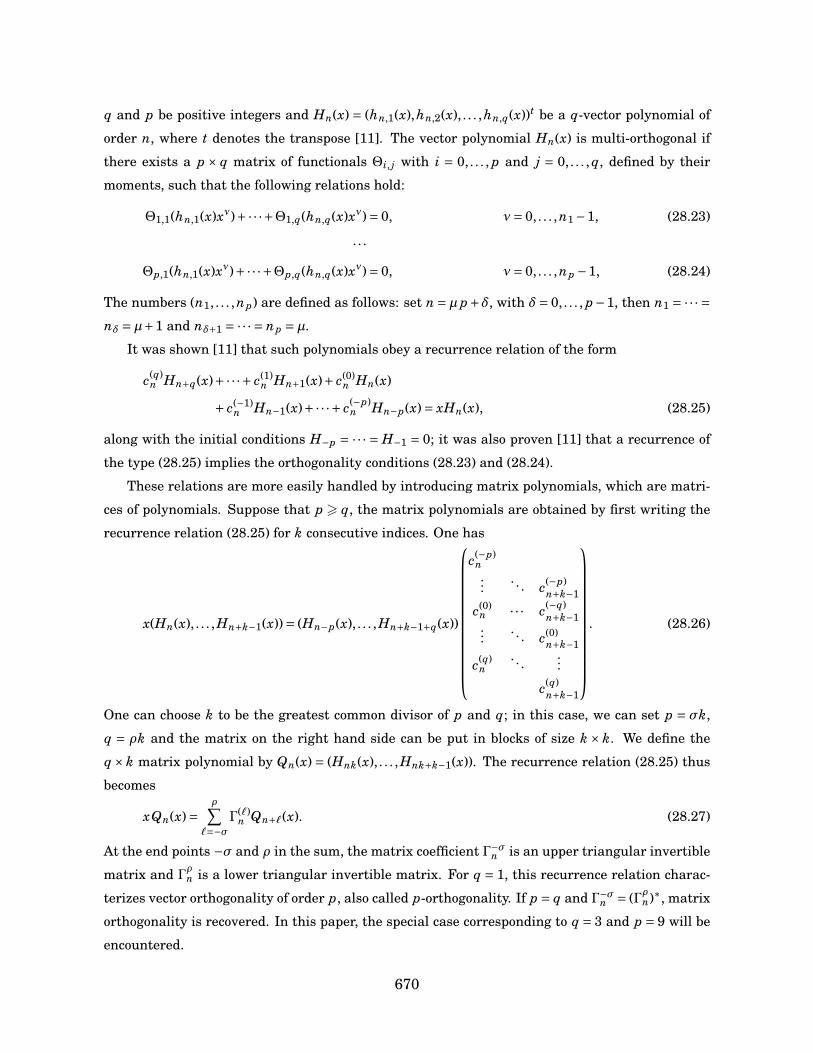
q and p be positive integers and Hn(x) = (hn,1(x),hn,2(x), . . . ,hn,q(x))t be a q-vector polynomial of
order n, where t denotes the transpose [11]. The vector polynomial Hn(x) is multi-orthogonal if
there exists a p× q matrix of functionals Θi, j with i = 0, . . . , p and j = 0, . . . , q, defined by their
moments, such that the following relations hold:
Θ1,1(hn,1(x)xν)+·· ·+Θ1,q(hn,q(x)xν)= 0, ν= 0, . . . ,n1 −1, (28.23)
· · ·Θp,1(hn,1(x)xν)+·· ·+Θp,q(hn,q(x)xν)= 0, ν= 0, . . . ,np −1, (28.24)
The numbers (n1, . . . ,np) are defined as follows: set n =µ p+δ, with δ= 0, . . . , p−1, then n1 = ·· · =nδ =µ+1 and nδ+1 = ·· · = np =µ.
It was shown [11] that such polynomials obey a recurrence relation of the form
c(q)n Hn+q(x)+·· ·+ c(1)
n Hn+1(x)+ c(0)n Hn(x)
+ c(−1)n Hn−1(x)+·· ·+ c(−p)
n Hn−p(x)= xHn(x), (28.25)
along with the initial conditions H−p = ·· · = H−1 = 0; it was also proven [11] that a recurrence of
the type (28.25) implies the orthogonality conditions (28.23) and (28.24).
These relations are more easily handled by introducing matrix polynomials, which are matri-
ces of polynomials. Suppose that p > q, the matrix polynomials are obtained by first writing the
recurrence relation (28.25) for k consecutive indices. One has
x(Hn(x), . . . ,Hn+k−1(x))= (Hn−p(x), . . . ,Hn+k−1+q(x))
c(−p)n...
. . . c(−p)n+k−1
c(0)n · · · c(−q)
n+k−1...
. . . c(0)n+k−1
c(q)n
. . ....
c(q)n+k−1
. (28.26)
One can choose k to be the greatest common divisor of p and q; in this case, we can set p = σk,
q = ρk and the matrix on the right hand side can be put in blocks of size k× k. We define the
q× k matrix polynomial by Qn(x) = (Hnk(x), . . . ,Hnk+k−1(x)). The recurrence relation (28.25) thus
becomes
xQn(x)=ρ∑
`=−σΓ(`)
n Qn+`(x). (28.27)
At the end points −σ and ρ in the sum, the matrix coefficient Γ−σn is an upper triangular invertible
matrix and Γρn is a lower triangular invertible matrix. For q = 1, this recurrence relation charac-
terizes vector orthogonality of order p, also called p-orthogonality. If p = q and Γ−σn = (Γρn)∗, matrix
orthogonality is recovered. In this paper, the special case corresponding to q = 3 and p = 9 will be
encountered.
670

28.1.5 Outline
The outline of the paper is as follows. In section 2, we obtain the recurrence relation satisfied by
the matrix elements Rk,n and show that they involve 3×3 matrix multi-orthogonal polynomials.
In section 3, we express these matrix elements as a finite convolution involving the Krawtchouk
polynomials and a family of 3-orthogonal polynomials recently studied in [3]. In section 4, we
obtain a biorthogonality relation for the matrix polynomials Qn(x). In section 5, we calculate the
matrix orthogonality functionals Θi, j for the polynomials. In section 6, we obtain a difference
equation for the polynomials and discuss the dual picture. In section 7, we derive the generating
functions and ladder relations. In section 8, we discuss the properties of the states | η,ξ ⟩ and study
spin squeezing in this system. In section 9, we briefly review the contraction limit N → ∞ and
relate our results with those of [13]. We close with concluding remarks in section 10. Appendices
containing su(2) structure formulas and properties of the Krawtchouk polynomials are included.
28.2 Recurrence relation
We shall begin the analysis by obtaining the recurrence relation satisfied by the matrix elements
Rk,n. We first observe that
(k−N/2)Rk,n = ⟨ k, N | J3R | N,n ⟩ = ⟨ k, N | RR−1J3R | N,n ⟩, (28.28)
where the inverse operator is given by
R−1 = eξ2 J2
− e−ξ2 J2
+ eηJ− e−µJ3 e−ηJ+ . (28.29)
The recurrence relation is obtained by expanding the expression R−1J3R and acting on the eigen-
states | N,n ⟩. This is done using the Baker–Campbell–Hausdorff relation
eABe−A = B+ [A,B]+ 12!
[A, [A,B]]+ 13!
[A, [A, [A,B]]]+ . . . , (28.30)
and the formulas for su(2) found in appendix A. Using the polar parametrizations η = ρeiδ and
ξ= reiγ, we obtain
R−1J3R = (1−2p)A0 +ρe−iδ(1− p)A−+ρ(1− p)[eiδ− re−i(δ−γ)]A+
+ (1−2p)reiγA 2+ −ρ r2e−i(δ−2γ)(1− p)A 3
+ −2ρ re−i(δ−γ)(1− p)A+A0 (28.31)
where we have defined
p = ρ2
1+ρ2 , A0 = J3 +ξJ2−, (28.32)
A− = J−, A+ = J+−ξ(1+2J3)J−−ξ2J3−. (28.33)
671
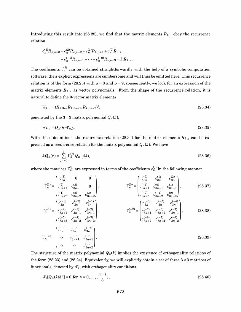
Introducing this result into (28.28), we find that the matrix elements Rk,n obey the recurrence
relation
c(3)n Rk,n+3 + c(2)
n Rk,n+2 + c(1)n Rk,n+1 + c(0)
n Rn,k
+ c(−1)n Rk,n−1 +·· ·+ c(−9)
n Rk,n−9 = k Rk,n.
The coefficients c( j)n can be obtained straightforwardly with the help of a symbolic computation
software, their explicit expressions are cumbersome and will thus be omitted here. This recurrence
relation is of the form (28.25) with q = 3 and p = 9; consequently, we look for an expression of the
matrix elements Rk,n as vector polynomials. From the shape of the recurrence relation, it is
natural to define the 3-vector matrix elements
Ψk,n = (Rk,3n,Rk,3n+1,Rk,3n+2)t, (28.34)
generated by the 3×3 matrix polynomial Qn(k),
Ψk,n =Qn(k)Ψk,0. (28.35)
With these definitions, the recurrence relation (28.34) for the matrix elements Rk,n can be ex-
pressed as a recurrence relation for the matrix polynomial Qn(k). We have
kQn(k)=1∑
j=−3Γ
( j)n Qn+ j(k), (28.36)
where the matrices Γ( j)n are expressed in terms of the coefficients c( j)
n in the following manner
Γ(1)n =
c(3)
3n 0 0
c(2)3n+1 c(3)
3n+1 0
c(1)3n+2 c(2)
3n+2 c(3)3n+2
, Γ(0)n =
c(0)
3n c(1)3n c(2)
3n
c(−1)3n+1 c(0)
3n+1 c(1)3n+1
c(−2)3n+2 c(−1)
3n+2 c(0)3n+2
, (28.37)
Γ(−1)n =
c(−3)
3n c(−2)3n c(−1)
3n
c(−4)3n+1 c(−3)
3n+1 c(−2)3n+1
c(−5)3n+2 c(−4)
3n+2 c(−3)3n+2
, Γ(−2)n =
c(−6)
3n c(−5)3n c(−4)
3n
c(−7)3n+1 c(−6)
3n+1 c(−5)3n+1
c(−8)3n+2 c(−7)
3n+2 c(−6)3n+2
, (28.38)
Γ(−3)n =
c(−9)
3n c(−8)3n c(−7)
3n
0 c(−9)3n+1 c(−8)
3n+1
0 0 c(−9)3n+2
. (28.39)
The structure of the matrix polynomial Qn(k) implies the existence of orthogonality relations of
the form (28.23) and (28.24). Equivalently, we will explicitly obtain a set of three 3×3 matrices of
functionals, denoted by Fi, with orthogonality conditions
Fi[Qn(k)kν]= 0 for ν= 0, . . . ,bn− i3
c, (28.40)
672
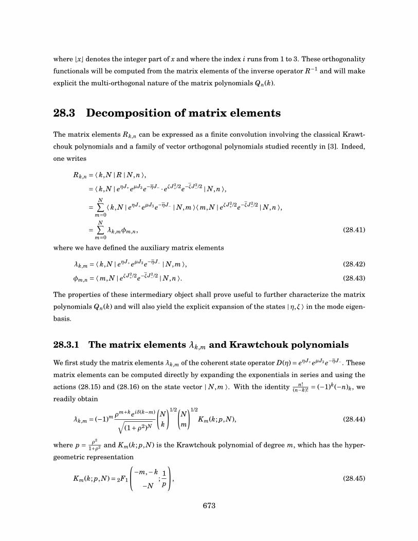
where bxc denotes the integer part of x and where the index i runs from 1 to 3. These orthogonality
functionals will be computed from the matrix elements of the inverse operator R−1 and will make
explicit the multi-orthogonal nature of the matrix polynomials Qn(k).
28.3 Decomposition of matrix elements
The matrix elements Rk,n can be expressed as a finite convolution involving the classical Krawt-
chouk polynomials and a family of vector orthogonal polynomials studied recently in [3]. Indeed,
one writes
Rk,n = ⟨ k, N | R | N,n ⟩,= ⟨ k, N | eηJ+ eµJ3 e−ηJ− · eξJ2
+/2e−ξJ2−/2 | N,n ⟩,
=N∑
m=0⟨ k, N | eηJ+ eµJ3 e−ηJ− | N,m ⟩⟨ m, N | eξJ2
+/2e−ξJ2−/2 | N,n ⟩,
=N∑
m=0λk,mφm,n, (28.41)
where we have defined the auxiliary matrix elements
λk,m = ⟨ k, N | eηJ+ eµJ3 e−ηJ− | N,m ⟩, (28.42)
φm,n = ⟨ m, N | eξJ2+/2e−ξJ2
−/2 | N,n ⟩. (28.43)
The properties of these intermediary object shall prove useful to further characterize the matrix
polynomials Qn(k) and will also yield the explicit expansion of the states | η,ξ ⟩ in the mode eigen-
basis.
28.3.1 The matrix elements λk,m and Krawtchouk polynomials
We first study the matrix elements λk,m of the coherent state operator D(η)= eηJ+ eµJ3 e−ηJ− . These
matrix elements can be computed directly by expanding the exponentials in series and using the
actions (28.15) and (28.16) on the state vector | N,m ⟩. With the identity n!(n−k)! = (−1)k(−n)k, we
readily obtain
λk,m = (−1)m ρm+keiδ(k−m)√(1+ρ2)N
(Nk
)1/2(Nm
)1/2
Km(k; p, N), (28.44)
where p = ρ2
1+ρ2 and Km(k; p, N) is the Krawtchouk polynomial of degree m, which has the hyper-
geometric representation
Km(k; p, N)= 2F1
−m,−k
−N;
1p
, (28.45)
673
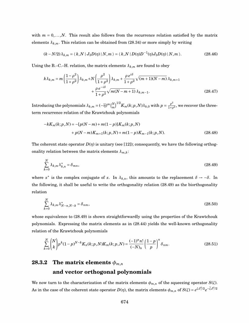
with m = 0, . . . , N. This result also follows from the recurrence relation satisfied by the matrix
elements λk,m. This relation can be obtained from (28.34) or more simply by writing
(k−N/2)λk,m = ⟨ k, N | J3D(η) | N,m ⟩ = ⟨ k, N | D(η)D−1(η)J3D(η) | N,m ⟩. (28.46)
Using the B.–C.–H. relation, the matrix elements λk,m are found to obey
kλk,m = m(
1−ρ2
1+ρ2
)λk,m+N
(ρ2
1+ρ2
)λk,m + ρ eiδ
1+ρ2
√(m+1)(N −m)λk,m+1
+ ρ e−iδ
1+ρ2
√m(N −m+1)λk,m−1. (28.47)
Introducing the polynomials λk,m = (−η)m(Nm
)1/2Km(k; p, N)λk,0 with p = ρ2
1+ρ2 , we recover the three-
term recurrence relation of the Krawtchouk polynomials
−kKm(k; p, N)=−[p(N −m)+m(1− p)]Km(k; p, N)
+ p(N −m)Km+1(k; p, N)+m(1− p)Km−1(k; p, N). (28.48)
The coherent state operator D(η) is unitary (see [12]); consequently, we have the following orthog-
onality relation between the matrix elements λm,k:
N∑k=0
λk,mλ∗k,n = δmn, (28.49)
where x∗ is the complex conjugate of x. In λk,n, this amounts to the replacement δ → −δ. In
the following, it shall be useful to write the orthogonality relation (28.49) as the biorthogonality
relation
N∑k=0
λk,mλ∗N−n,N−k = δnm, (28.50)
whose equivalence to (28.49) is shown straightforwardly using the properties of the Krawtchouk
polynomials. Expressing the matrix elements as in (28.44) yields the well-known orthogonality
relation of the Krawtchouk polynomials
N∑k=0
(Nk
)pk(1− p)N−kKn(k; p, N)Km(k; p, N)= (−1)nn!
(−N)n
(1− p
p
)nδnm. (28.51)
28.3.2 The matrix elements φm,n
and vector orthogonal polynomials
We now turn to the characterization of the matrix elements φm,n of the squeezing operator S(ξ).
As in the case of the coherent state operator D(η), the matrix elements φm,n of S(ξ)= eξJ2+/2e−ξJ2
−/2
674
can be computed directly by expanding the exponentials in series and applying the actions (28.15)
and (28.16) on the state vector | N,n ⟩. Obviously, any matrix element φm′,n′ with m′ and n′ of
different parities will be zero; consequently, we set n = 2a+ c and m = 2b+ c with c = 0,1 and
obtain
φm,n = (−1)a (r/2)a+beiγ(b−a)
a!b!
√(N − c)!m!(N −m)!
√(N − c)!n!(N −n)!
A(c)a (b;d, N), (28.52)
where the identities (a)2n = 22n ( a2)n
( a+12
)n and (2σ+ s)! = 22σs!σ!(s+1/2)σ were used and where
we have defined
A(c)a (b;d, N)= 2F3
−a −b
c+1/2 c−N2
c−N+12
;1d
, (28.53)
with d =−4r2. The polynomials A(c)a have been studied in [3]; we review here some basic results.
The polynomials A(c)a are vector orthogonal polynomials of dimension 3, which corresponds to the
case q = 1 and p = 3 of the general setting presented in the introduction. This can be seen by
computing the recurrence relation satisfied by the matrix elements φm,n. Once again, we start
with
(m−N/2)φm,n = ⟨ m, N | J3S(ξ) | N,n ⟩ = ⟨ m, N | S(ξ)S−1(ξ)J3S(ξ) | N,n ⟩. (28.54)
Using the B.–C.–H. relation and the formulas from Appendix A, we obtain
S−1(ξ)J3S(ξ)= (J3 +ξJ2−)+ξ[J+−ξ(1+2J3)J−−ξ2
J3−]2. (28.55)
Substituting this result into (28.54) yields
(m−n)φm,n = ξ√
(n+1)2(n−N)2φm,n+2 +ξ√
(−n)2(N −n+1)2φm,n−2
+ξξ3∑
j=0ξ
j√(−n)2 j(N −n+1)2 j f ( j)
n φm,n−2 j, (28.56)
with coefficients
f (0)n = (N −2n)(−1+N +2Nn−2n2), (28.57)
f (1)n = (6n2 −12n+N(5−6n)+N2 +9), (28.58)
f (2)n = (4n−2N −8), (28.59)
f (3)n = 1. (28.60)
Setting φ2b+c,2a+c = (−ξ)a
a!
√(N−c)!n!(N−n)! A(c)
a (b;d, N)φ2b+c,c, the polynomials A(c)a (b;d, N) are seen to
obey the recurrence relation
(b−a)A(c)a (b;d, N)= −ξξ
a+1(n+1)2(n−N)2 A(c)
a+1(b;d, N)−aA(c)a−1(b;d, N)
+ξξ3∑
j=0(−a) j f ( j)
n A(c)a− j(b;d, N). (28.61)
675
The matrix elements φm,n are thus given by two families of polynomials A(c)a for c = 0,1 of vector
orthogonal polynomials of order 3. The matrix elements of the inverse operator S−1(ξ) can also
be found by direct computation or by inspection. One readily sees that the matrix elements φm,n
obey the biorthogonality relation
N∑m=0
φm,nφ∗N−n′,N−m = δnn′ , (28.62)
In contrast to the situation with the matrix elements λk,m of the displacement operator D(η), the
biorthogonality relation for the matrix elements φm,n is not equivalent to a standard orthogonality
relation; this is a consequence of the non-unitarity of S(ξ) and explains the vector-orthogonal
nature of the polynomials A(c)a (b;d, N). From the biorthogonality relation of the matrix elements
φm,n follow two biorthogonality relations for the polynomials A(c)a (b;d, N); we have, for N = 2u+2c,
u∑b=0
(−1)b
(ub
)A(c)
a (b;d, N)A(c)u−a′(u−b;d, N)= a!
(−u)a[(c+1/2)u]2
(1d
)uδaa′ . (28.63)
For N = 2u+1, we find a biorthogonality relation interlacing the two families c = 0 and c = 1:
u∑b=0
(−1)b
(ub
)A(1)
a (b;d, N)A(0)u−a′(u−b;d, N)= a!
(−u)a[(1/2)u(3/2)u]
(1d
)uδaa′ . (28.64)
28.3.3 Full matrix elements and squeezed-coherent states
The results of the two preceding subsections allow to write explicitly the matrix elements Rk,n;
noting that φm,n is automatically zero when m and n have different parities, we have, for n = 2a+c,
the following expression for the full matrix elements:
Rk,n =Φb N−c
2 c∑b=0
ΘbK2b+c(k; p, N)A(c)a (b;d, N), (28.65)
where we have defined
Φ= 1√(1+ρ2)N
ηk(−ξ/2)a
a!
(Nk
)1/2√(N − c)!n!(N −n)!
, (28.66)
Θb =(−η)2b+c(ξ/2)b
b!
(N
2b+ c
)1/2√(N − c)!(2b+ c)!
(N −2b− c)!. (28.67)
The generalized squeezed-coherent states are therefore expressed as the linear combination
| η,ξ ⟩n = 1Norm
N∑k=0
Rk,n| N,k ⟩, (28.68)
676
where Norm is a normalization constant. The expression for the amplitudes simplifies signifi-
cantly if one considers the standard squeezed-coherent states in which the operator R(η,ξ) acts on
the vacuum. Indeed, we have
| η,ξ ⟩ = 1Norm
N∑k=0
√1
(1+ρ2)N
(Nk
)1/2
ηk
b N2 c∑
b=0
(η2ξ/2)b
b!(−N)2bK2b(k; p, N)
| k ⟩. (28.69)
If the squeezing parameter ξ= reiγ is set to zero, we recover the standard normalized su(2) coher-
ent states
| η ⟩ =√
1(1+ρ2)N
N∑k=0
(Nk
)1/2
ηk| k ⟩. (28.70)
In section 8, the properties of the states | η,ξ ⟩ will be further investigated; in particular, it will be
shown that they exhibit spin squeezing when N is even.
28.4 Biorthogonality relation
Given the symmetry of the matrix elements entering the finite convolution yielding Rk,n, the
matrix elements of the inverse operator S−1(ξ)D−1(η) are expected to have a similar behavior.
Indeed, one finds thatN∑
k=0Rk,nRN−k,N−n′ = δnn′ , (28.71)
where ∼ denotes the replacements ρ→−ρ and r →−r. In terms of the vector polynomials Ψk,n =(Rk,3n,Rk,3n+1,Rk,3n+2)t, this biorthogonality relation takes the form
N∑k=0
Ψk,n(ΨN−k,N−n′)t = δnn′Id3×3. (28.72)
This equation can be transformed into a biorthogonality relation for the matrix polynomials Qn(k).
Indeed, one hasN∑
k=0Qn(k)Ψk,0(QN−n′(N −k)ΨN−k,0)t = δnn′Id3×3, (28.73)
which can be written asN∑
k=0Qn(k)W(k)(QN−n′(N −k))t = δnn′Id3×3, (28.74)
with the biorthogonality weight matrix
W(k)=
Rk,0RN−k,0 Rk,0RN−k,1 Rk,0RN−k,2
Rk,1RN−k,0 Rk,1RN−k,1 Rk,1RN−k,2
Rk,2RN−k,0 Rk,2RN−k,1 Rk,2RN−k,2
. (28.75)
Each element of the weight matrix can be computed exactly as a finite sum with the help of the
equation (28.65).
677
28.5 Matrix Orthogonality functionals
From the recurrence relation (28.34) and the results in [11], it is known that there exists a set of
three 3×3 matrix of functionals with respect to which the matrix polynomials Qn(k) are orthog-
onal. To construct these functionals, we consider the recurrence relation satisfied by the matrix
elements of the inverse operator R−1(η,ξ). These matrix elements are defined as
R−1n,k = ⟨ n, N | R−1 | N,k ⟩, (28.76)
and their recurrence relation is obtained by noting that
(k−N/2)R−1n,k = ⟨ n, N | R−1J0 | N,k ⟩ = ⟨ n, N | R−1J0RR−1 | N,k ⟩. (28.77)
The quantity R−1J3R has been computed previously; recalling that J†± = J∓ and that J†
3 = J3, the
recurrence relation for the inverse 3-vector Ψ−1n,k is given by
kΨ−1n,k =
3∑j=−1
e( j)n Ψ
−1n+ j,k, (28.78)
where the coefficients e( j)n are 3×3 matrices and e(−1)
n as well as e(3)n are respectively lower and
upper triangular invertible matrices. Since
N∑k=0
R−1m,kRk,n =
N∑k=0
⟨ m, N | R−1 | N,k ⟩⟨ k, N | R | N,n ⟩ = δnm, (28.79)
it follows that
N∑k=0
Ψk,n(Ψ−1m,k)t = δnmId3×3. (28.80)
We may now state the following proposition.
Proposition 14. The 3-vector Ψ−1n,k can be expressed as
Ψ−1n,k =
2∑i=0
p(n)i (k)κiΞi, (28.81)
where Ξi =Ψ−1i,k. The κi are 3×3 matrices which depend only on i and p(n)
i (k) are polynomials in the
variable k. Let n = 3ν+`, for `= 0,1,2; if i 6 `, the degree of the polynomial p(n)i (k) is ν, otherwise
it is ν−1.
Proof. We set n = 0 in the recurrence relation (28.78), which leads to
e(3)n Ψ−1
3,k = (k Id3×3 − e(0)0 )Ψ−1
0,k − e(1)Ψ−11,k − e(2)Ψ−1
2,k. (28.82)
678

Since e(3)n is upper triangular and invertible, it follows that
Ψ−13,k =
2∑i=0
p(3)i (k)κiΨ
−1i,k, (28.83)
where the degree of p(3)i (k) is 1 for i = 0 and 0 for all other indices. This establishes (28.81) for
n = 0. The proof is then completed by induction.
From this proposition, it is natural to define the following matrices of functionals.
Definition 16. Let Fi for i = 1,2,3 be the matrix functionals defined by
Fi[·]=N∑
k=0[·]Ψk,0Ξ
ti−1. (28.84)
With this definition, the relation (28.80) can be written as
Fi[kνQn(k)]= 03×3 for ν= 0, . . . ,bn− i3
c, (28.85)
for i = 1,2,3. The multi-orthogonality of the matrix polynomials Qn(k) has thus been made explicit
by the direct construction of the orthogonality functionals.
28.6 Difference equation
The matrix polynomials Qn(k) are bi-spectral; not only do they satisfy a recurrence relation, they
also obey a difference equation. In a fashion dual to the approach followed to find the recurrence
relation, we observe that
(n−N/2)Rk,n = ⟨ k, N | RJ3 | N,n ⟩ = ⟨ k, N | RJ3R−1R | N,n ⟩. (28.86)
Using once again the B.–C.–H relation and formulas from appendix A, we obtain
RJ3R−1 = (B0 −ξB2+)−ξ[B−+ξB+(1+2B0)−ξ2B3
+]2, (28.87)
with
B0 = (1−2p)J3 −ρeiδ(1− p)J+−ρe−iδ(1− p)J−, (28.88)
B+ = (1− p)J++2ρe−iδ(1− p)J3 − pe−2iδJ−, (28.89)
B− =−pe2iδJ++2ρeiδ(1− p)J3 + (1− p)J−. (28.90)
Expanding these expressions leads to a difference equation of the form
nRk,n =6∑
j=−6m( j)
k Rk+ j,n, (28.91)
679

which can be turned into a difference equation for the matrix polynomials Qn(k) which is quite
involved and not provided here.
It is interesting to observe that this difference equation contains the same number of terms
as the recurrence relation, but has a different symmetry. Indeed, the indices run from −6 to 6 in
the difference equation. It indicates that the order in which the coherent state operator and the
squeezing operator are presented has an impact on the structure of the associated polynomials.
If one defines R′ = S(ξ)D(η) instead of R = D(η)S(ξ), one gets 6×6 matrix multi-orthogonal poly-
nomials satisfying a three-term matrix recurrence relation; these polynomials are not, however,
orthogonal, because the condition (Γ(−6)n )∗ =Γ(6)
n is not fulfilled.
28.7 Generating functions and ladder relations
The ordinary su(2) coherent states | η ⟩ can be used to obtain a generating function for the matrix
elements Rk,n. We consider the two-variable function defined by
G(x, y)= 1(1+ρ2)N
∑k,n
(Nk
)1/2(Nn
)1/2
xk ynRk,n. (28.92)
Clearly, the function G(x, y) can be viewed as the matrix element of R between the coherent states
| x ⟩ and | y ⟩. Introducing a resolution of the identity, we obtain
G(x, y)= ⟨ x | R | y ⟩ =N∑
m=0⟨ x | D(η) | N,m ⟩⟨ m, N | S(ξ) | y ⟩. (28.93)
The first part of this convolution can be evaluated directly using the action of the generators J±on the states; not surprisingly, we recover, up to a multiplicative factor, the generating function of
the Krawtchouk polynomials; the result is
⟨ x | D(η) | N,m ⟩ = ηm
(1+ρ2)N
(Nm
)1/2
(1+ηx)N−m(
(1− p)p
ηx−1)m
, (28.94)
with p = ρ2
1+ρ2 . The second part in the R.H.S of (28.93) is also readily determined. Setting m = 2t+s,
one finds
⟨ m, N | S(ξ) | y ⟩ = ξt ys
t!
√N!m!
(N −m)!
b N−s2 c∑
k=0
(−y2/ξ)k
(2k+ s)!(−t)k 2F0
(−z(k)2
,1− z(k)
2;−4y2ξ
), (28.95)
where z(k) = N −2k− s. The convolution of the two functions given in (28.94) and (28.95) thus
yields the generating function for the matrix elements Rk,n. The ladder relations for the matrix
polynomials Qn(k) can also be constructed explicitly from the observations√−(n+1)3(n−N)3 Rk,n+3 = ⟨ k, N | RJ3
+ | N,n ⟩,√−(−n)3(N −n+1)3 Rk,n−3 = ⟨ k, N | RJ3
− | N,n ⟩. (28.96)
680
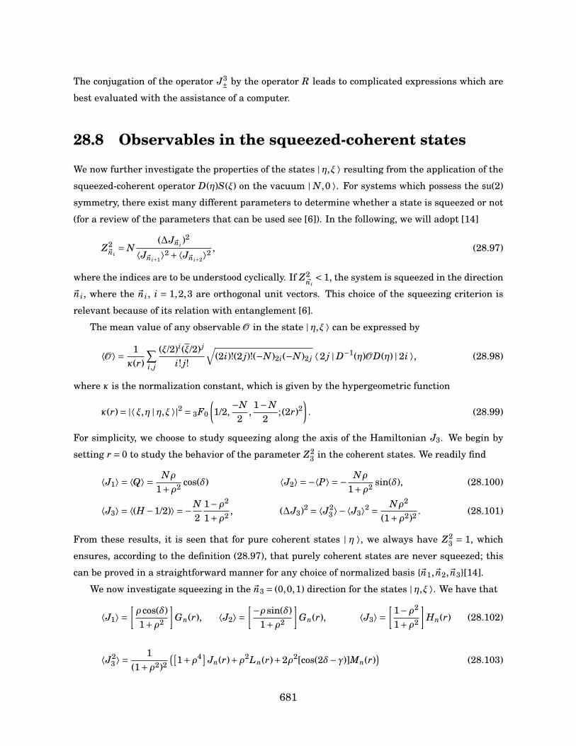
The conjugation of the operator J3± by the operator R leads to complicated expressions which are
best evaluated with the assistance of a computer.
28.8 Observables in the squeezed-coherent states
We now further investigate the properties of the states | η,ξ ⟩ resulting from the application of the
squeezed-coherent operator D(η)S(ξ) on the vacuum | N,0 ⟩. For systems which possess the su(2)
symmetry, there exist many different parameters to determine whether a state is squeezed or not
(for a review of the parameters that can be used see [6]). In the following, we will adopt [14]
Z2~ni
= N(∆J~ni )
2
⟨J~ni+1⟩2 +⟨J~ni+2⟩2, (28.97)
where the indices are to be understood cyclically. If Z2~ni< 1, the system is squeezed in the direction
~ni, where the ~ni, i = 1,2,3 are orthogonal unit vectors. This choice of the squeezing criterion is
relevant because of its relation with entanglement [6].
The mean value of any observable O in the state | η,ξ ⟩ can be expressed by
⟨O⟩ = 1κ(r)
∑i, j
(ξ/2)i(ξ/2) j
i! j!
√(2i)!(2 j)!(−N)2i(−N)2 j ⟨ 2 j | D−1(η)OD(η) | 2i ⟩, (28.98)
where κ is the normalization constant, which is given by the hypergeometric function
κ(r)= |⟨ ξ,η | η,ξ ⟩|2 = 3F0
(1/2,
−N2
,1−N
2;(2r)2
). (28.99)
For simplicity, we choose to study squeezing along the axis of the Hamiltonian J3. We begin by
setting r = 0 to study the behavior of the parameter Z23 in the coherent states. We readily find
⟨J1⟩ = ⟨Q⟩ = Nρ
1+ρ2 cos(δ) ⟨J2⟩ =−⟨P⟩ =− Nρ
1+ρ2 sin(δ), (28.100)
⟨J3⟩ = ⟨(H−1/2)⟩ =−N2
1−ρ2
1+ρ2 , (∆J3)2 = ⟨J23 ⟩−⟨J3⟩2 = Nρ2
(1+ρ2)2 . (28.101)
From these results, it is seen that for pure coherent states | η ⟩, we always have Z23 = 1, which
ensures, according to the definition (28.97), that purely coherent states are never squeezed; this
can be proved in a straightforward manner for any choice of normalized basis ~n1,~n2,~n3[14].
We now investigate squeezing in the ~n3 = (0,0,1) direction for the states | η,ξ ⟩. We have that
⟨J1⟩ =[ρ cos(δ)1+ρ2
]Gn(r), ⟨J2⟩ =
[−ρ sin(δ)1+ρ2
]Gn(r), ⟨J3⟩ =
[1−ρ2
1+ρ2
]Hn(r) (28.102)
⟨J23 ⟩ =
1(1+ρ2)2
([1+ρ4]
Jn(r)+ρ2Ln(r)+2ρ2[cos(2δ−γ)]Mn(r))
(28.103)
681
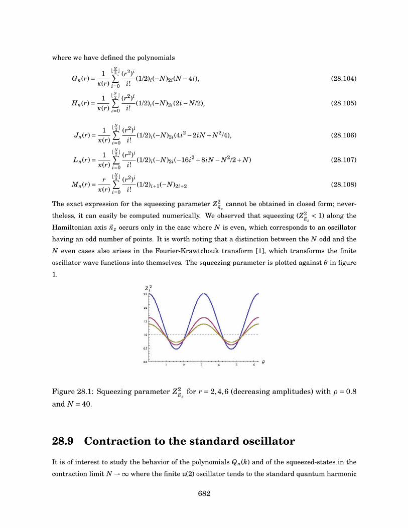
where we have defined the polynomials
Gn(r)= 1κ(r)
b N2 c∑
i=0
(r2)i
i!(1/2)i(−N)2i(N −4i), (28.104)
Hn(r)= 1κ(r)
b N2 c∑
i=0
(r2)i
i!(1/2)i(−N)2i(2i−N/2), (28.105)
Jn(r)= 1κ(r)
b N2 c∑
i=0
(r2)i
i!(1/2)i(−N)2i(4i2 −2iN +N2/4), (28.106)
Ln(r)= 1κ(r)
b N2 c∑
i=0
(r2)i
i!(1/2)i(−N)2i(−16i2 +8iN −N2/2+N) (28.107)
Mn(r)= rκ(r)
b N2 c∑
i=0
(r2)i
i!(1/2)i+1(−N)2i+2 (28.108)
The exact expression for the squeezing parameter Z2~nz
cannot be obtained in closed form; never-
theless, it can easily be computed numerically. We observed that squeezing (Z2~nz
< 1) along the
Hamiltonian axis ~nz occurs only in the case where N is even, which corresponds to an oscillator
having an odd number of points. It is worth noting that a distinction between the N odd and the
N even cases also arises in the Fourier-Krawtchouk transform [1], which transforms the finite
oscillator wave functions into themselves. The squeezing parameter is plotted against θ in figure
1.
Figure 28.1: Squeezing parameter Z2~nz
for r = 2,4,6 (decreasing amplitudes) with ρ = 0.8
and N = 40.
28.9 Contraction to the standard oscillator
It is of interest to study the behavior of the polynomials Qn(k) and of the squeezed-states in the
contraction limit N →∞ where the finite u(2) oscillator tends to the standard quantum harmonic
682
oscillator; this limit was studied in detail in [2]. To obtain the proper limit, the parameters of the
squeeze-coherent operator must be renormalized according to
ρ→ ρpN
, r → rN
. (28.109)
Upon taking the limit, one finds that the 13-term recurrence relation of the Rn,k tends to a 5-term
symmetric recurrence relation of the form
kRk,n =2∑
j=−2c( j)
n Rk,n+ j. (28.110)
This is indeed the type of recurrence relation obtained in [13]. In the case of the standard oscillator,
it is possible to choose a unitary version of the corresponding S operator and to express its matrix
elements in terms of 2×2 matrix orthogonal polynomials.
28.10 Conclusion
The matrix elements of the exponential operators corresponding to the squeezed-coherent opera-
tors of the finite oscillator have been determined in the energy eigenbasis of this model. They were
seen to be given in terms of matrix multi-orthogonal polynomials which have the Krawtchouk and
vector orthogonal polynomials as building blocks. The algebraic setting allowed to characterize
these polynomials and to explicitly compute their matrix orthogonality functionals. The results
have been used to show that the squeezed coherent states of the finite oscillator exhibit squeezing
when the dimension of the oscillator N +1 is odd.
Appendix A–Useful formulas involving the su(2) gener-
ators
The relation
J3Jn± = Jn
±(J3 ±n),
holds and can be proven straightforwardly by induction on n. Using this identity and the relations
(J±)† = J∓ as well as J†3 = J3 , it follows that for P(J±) denoting a polynomial in J±, one has
[P(J±), J3]=∓J±P ′(J±),
where P ′(x) is the derivative of P(x) with respect to x. The preceding formula and the Baker-
Campbell-Hausdorff relation lead to the identity
eP(J±)J3e−P(J±) = J3 ∓ J±P ′(J±).
683
In addition, we have the relations
[J+, Jn−]= 2nJ3Jn−1
− +n(n−1)Jn−1− ,
[J−, Jn+]=−2nJn−1
+ J3 −n(n−1)Jn−1+ ,
which can also be proved by induction on n. With the help of the previous identities, one obtains
[J+,P(J−)]= 2J3P ′(J−)+ J−P ′′(J−),
[J−,P(J+)]=−2P ′(J+)J3 − J+P ′′(J+),
From these formulas it follows that
eP(J−)J+e−P(J−) = J+−2J3P ′(J−)− J−[P ′′(J−)+P ′(J−)2],
eP(J+)J−e−P(J+) = J−+2P ′(J+)J3 + J+[P ′′(J+)−P ′(J+)2].
Appendix B–Krawtchouk polynomials
The Krawtchouk polynomials have the hypergeometric representation
Kn(x; p, N)= 2F1
−n,−x
−N;
1p
.
Their orthogonality relation is
N∑x=0
(Nx
)px(1− p)N−xKm(x; p, N)Kn(x; p, N)= (−1)nn!
(−N)n
(1− p
p
)nδnm.
They have the generating function
(1+ t)N−x(1− 1− p
pt)x
=N∑
n=0
(Nn
)Kn(x; p, N)tn.
For further details, see [4].
References[1] N.M. Atakishiyev, G.S. Pogosyan, L.E. Vicent, and K.B. Wolf. Finite two-dimensional oscilla-
tor I: The cartesian model. Journal of Physics A: Mathematical and General, 34:9381–9398,
2001.
[2] N.M. Atakishiyev, G.S. Pogosyan, and K.B. Wolf. Contraction of the finite one-dimensional
oscillator. International Journal of Modern Physics A, 18:317–327, 2003.
684
[3] V.X. Genest, L. Vinet, and A. Zhedanov. d-Orthogonal polynomials and su(2). Journal of
Mathematical Analysis and Applications, 390:472–487, 2012.
[4] R. Koekoek, P.A. Lesky, and R.F. Swarttouw. Hypergeometric orthogonal polynomials and
their q-analogues. Springer, 1st edition, 2010.
[5] G. Labahn and B. Beckermann. A uniform approach for Hermite-Padé and simultaneous
Padé approximants and their matrix type generalization. Numerical Algorithms, 3:45–54,
1992.
[6] J. Ma, X. Wang, C.P. Sun, and F. Nori. Quantum spin squeezing. Physics Reports, (509):89–
165, 2011.
[7] S. Massar and P. Spindel. Uncertainty relation for the discrete fourier transform. Phys. Rev.
Lett., 100:190401, 2008.
[8] U. Niederer. The maximal kinematical invariance group of the free Schrödinger equations.
Helvetica Physica Acta, 45:802–810, 1972.
[9] U. Niederer. Maximal kinematical invariance group of the harmonic oscillator. Helvetica
Physica Acta, 46:191–200, 1973.
[10] M.V. Satyanarayana. Generalized coherent states and generalized squeezed coherent states.
Physical Review D, 32:400–404, 1985.
[11] V.N. Sorokin and J. Van Iseghem. Algebraic aspects of matrix orthogonality for vector poly-
nomials. Journal of Approximation Theory, 90:97–116, 1997.
[12] D.R. Truax. Baker-Campbell-Hausdorff relations and unitarity of su(2) and su(1,1) squeeze
operators. Physical Review D, 31:1988–1991, 1985.
[13] L. Vinet and A. Zhedanov. Representations of the Schrödinger group and matrix orthogonal
polynomials. Journal of Physics A: Mathematical and Theoretical, 44(35):1–28, 2011.
[14] X. Wang. Spin squeezing in nonlinear spin-coherent states. Journal of Optics B: Quantum
and Semiclassical Optics, 3:93–96, 2001.
[15] E.P. Wigner and E. Inönü. On the contraction of groups and their representations. Proceed-
ings of the National Academic Society, 39:510–524, 1956.
[16] K.B. Wolf and G. Krötzsch. Geometry and dynamics of squeezing in finite systems. Journal
of the Optical Society of America, 24:2871–2878, 2007.
685

686
Conclusion
En guise de conclusion, je propose ici quelques questions de recherche liées émanant directement
de la présente thèse et qui mériteraient sans doute d’être étudiées.
• La dualité de Schur-Weyl classique établit un lien entre les n-uplets de produits tensoriels
de représentations de sl2 et l’algèbre du groupe symétrique CSn. Des versions de cette
dualité existent entre les algèbres quantiques Uq(sl2), ospq(1|2) et la superalgèbre osp(1|2)
et les algèbres de Hecke, de Birman–Murakami–Wenzl et Brauer. Il serait intéressant de
déterminer le lien entre ces algèbres et les algèbres de Racah, Bannai–Ito, Askey–Wilson et
q-Bannai–Ito.
• Les algèbres de Racah, de Bannai–Ito, de Askey–Wilson et q-Bannai–Ito peuvent être vues
comme des algèbres quadratiques de rang 1. Il serait naturel d’en obtenir des généralisa-
tions au rang n et de déterminer leurs liens avec les polynômes orthogonaux multivariés.
• Nous avons étudié un certain nombre de systèmes superintégrables en n dimension constru-
its à l’aide des opérateurs de Dunkl associés au système de racine A×n1 . Il serait pertinent
d’examiner des systèmes définis en termes des opérateurs de Dunkl associés à d’autres sys-
tèmes de racines.
• Il serait utile d’obtenir des généralisations à multivariées des polynômes du tableau de
Bannai–Ito et de comprendre leurs liens avec les systèmes superintégrables avec réflexions
en plus hautes dimensions.
• Une q-généralisation des relations entre les groupes SO(d+1), SO(d,1), E(d) et les familles
de polynômes multivariés de Krawtchouk, Meixner et Charlier serait désirable. Elle perme-
tterait de caractériser davantage certaines familles de q-polynômes multivariés proposés
par Gasper et Rahman.
687

688
Contribution aux articles
Cette annexe vise à détailler la contribution de VXG aux articles compris dans cette thèse, confor-
mément aux exigences de la FESP. La description est sommaire. Les contributions sous la forme
de commentaires, discussions, suggestions, etc., ne sont pas mentionnées.
• Chapitre 1. Idée originale et première version par AZ et LV. Réécriture complète et ajouts
subtantiels par LV et VXG. Calculs par AZ, VXG et LV.
• Chapitre 2. Idée originale de LV et VXG. Rédaction et calculs par VXG.
• Chapitre 3. Idée originale de HM, LV et VXG. Rédaction et calculs par VXG.
• Chapitre 4. Idée originale de LV. Rédaction et calculs par VXG.
• Chapitre 5. Idée originale, rédaction et calculs par VXG.
• Chapitre 6. Idée originale, rédaction et calculs par VXG.
• Chapitre 7. Idée originale de LV et VXG. Calculs par VXG et LV. Rédaction par VXG.
• Chapitre 8. Idée originale de LV. Calculs par VXG et LV. Rédaction par VXG.
• Chapitre 9. Idée originale de LV et VXG. Calculs par JG, JL et VXG. Rédaction par VXG.
• Chapitre 10. Idée originale de LV et MI. Calculs par LV et VXG. Rédaction par VXG et LV.
• Chapitre 11. Idée originale de LV. Calculs et rédaction par VXG.
• Chapitre 12. Idée originale de LV et VXG. Calculs et rédaction par VXG.
• Chapitre 13. Idée originale par VXG. Calculs et rédaction par VXG.
• Chapitre 14. Idée originale par LV, AZ et VXG. Calculs et rédaction par VXG.
• Chapitre 15. Idée originale par LV. Calculs par VXG, HDB et LV. Rédaction par VXG.
• Chapitre 16. Idée originale par AZ et LV. Calculs par AZ et VXG. Rédaction par VXG.
689
• Chapitre 17. Idée originale par AZ, LV et VXG. Calculs et rédaction par VXG.
• Chapitre 18. Idée originale par LV. Calculs et rédaction par VXG.
• Chapitre 19. Idée originale, calculs et rédaction par VXG.
• Chapitre 20. Idée originale par LV. Rédaction par VXG.
• Chapitre 21. Idée originale par LV et VXG. Calculs et rédaction par VXG.
• Chapitre 22. Idée originale, calculs et rédaction par VXG.
• Chapitre 23. Idée originale par AZ. Calculs par AZ, LV et VXG. Rédaction par VXG et AZ.
• Chapitre 24. Idée originale par LV, AZ et VXG. Calculs par AZ. Rédaction par VXG et LV.
• Chapitre 25. Idée originale et calculs par LV et VXG. Rédaction par LV et VXG.
• Chapitre 26. Idée originale par VXG, AZ et LV. Calculs et rédaction par VXG.
• Chapitre 27. Idée originale par LV et AZ. Calculs et rédaction par VXG.
• Chapitre 28. Idée originale par LV et AZ. Calculs et rédaction par VXG.
690
Bibliographie
[1] L. D. Landau et E. M. Lifshitz, Mechanics. Butterworth-Heinemann, 1976.
[2] C. Cohen-Tannoudji, B. Diu, et F. Laloë, Mécanique quantique I. Hermann, 1997.
[3] S. Karlin et J. McGregor, “The Hahn polynomials, formulas and an application,” Scripta
Mathematica, vol. 45, pp. 176–198, 1974.
[4] W. Greiner et D. A. Bromley, Relativistic Quantum Mechanics. Wave Equations. Springer,
2000.
[5] W. Greiner, J. Reinhardt, et D. Bromley, Field Quantization. Springer, 1996.
[6] A. F. Nikiforov, S. K. Suslov, et V. B. Uvarov, Classical Orthogonal Polynomials of a Discrete
Variable. Springer, 1991.
[7] V. X. Genest, L. Vinet, et A. Zhedanov, “The multivariate Krawtchouk polynomials as matrix
elements of the rotation group representations on oscillator states,” Journal of Physics A:
Mathematical and Theoretical, vol. 46, p. 505203, 2013.
[8] V. X. Genest, H. Miki, L. Vinet, et A. Zhedanov, “The multivariate Meixner polynomials as
matrix elements of SO(d,1) representations on oscillator states,” Journal of Physics A: Math-
ematical and Theoretical, vol. 47, p. 045207, 2014.
[9] V. X. Genest, H. Miki, L. Vinet, et A. Zhedanov, “The multivariate Charlier polynomials
as matrix elements of the Euclidean group representation on oscillator states,” Journal of
Physics A: Mathematical and Theoretical, vol. 47, p. 215204, 2014.
[10] V. X. Genest, L. Vinet, et A. Zhedanov, “Interbasis expansions for the isotropic 3D harmonic
oscillator and bivariate Krawtchouk polynomials ,” Journal of Physics A: Mathematical and
Theoretical, vol. 47, p. 025202, 2014.
691
[11] V. X. Genest et L. Vinet, “The multivariate Hahn polynomials and the singular oscillator,”
Journal of Physics A: Mathematical and Theoretical, vol. 47, p. 455201, 2014.
[12] V. X. Genest et L. Vinet, “The Generic Superintegrable System on the 3-Sphere and the 9 j
Symbols of su(1,1),” SIGMA, vol. 10, p. 108, 2014.
[13] V. X. Genest, S. Post, L. Vinet, G.-F. Yu, et A. Zhedanov, “q-rotations and Krawtchouk poly-
nomials,” The Ramanujan Journal, 2015.
[14] V. X. Genest, H. Miki, L. Vinet, et A. Zhedanov, “Spin lattices, state transfer and bivariate
Krawtchouk polynomials ,” ArXiv:1410.4703, 2015.
[15] J. Gaboriaud, V. X. Genest, J. Lemieux, et L. Vinet, “A superintegrable discrete oscillator and
two-variable Meixner polynomials ,” ArXiv:1502.07293, 2015.
[16] V. X. Genest, M. Ismail, L. Vinet, et A. Zhedanov, “The Dunkl oscillator in the plane: I.
Superintegrability, separated wavefunctions and overlap coefficients,” Journal of Physics A:
Mathematical and Theoretical, vol. 46, p. 145201, 2013.
[17] V. X. Genest, M. Ismail, L. Vinet, et A. Zhedanov, “The Dunkl Oscillator in the Plane II: Rep-
resentations of the Symmetry Algebra,” Communications in Mathematical Physics, vol. 329,
pp. 999–1029, 2014.
[18] V. X. Genest, L. Vinet, et A. Zhedanov, “The singular and the 2:1 anisotropic Dunkl oscillators
in the plane ,” Journal of Physics A: Mathematical and Theoretical, vol. 46, p. 325201, 2013.
[19] V. X. Genest, L. Vinet, et A. Zhedanov, “The Dunkl oscillator in three dimensions ,” Journal
of Physics: Conference Series, vol. 512, p. 012010, 2014.
[20] V. X. Genest, L. Vinet, et A. Zhedanov, “The Bannai–Ito algebra and a superintegrable system
with reflections on the two-sphere,” Journal of Physics A: Mathematical and Theoretical,
vol. 47, p. 205202, 2014.
[21] H. De Bie, V. X. Genest, et L. Vinet, “A Dirac-Dunkl equation on S2 and the Bannai-Ito
algebra,” ArXiv:1501.03108, 2015.
[22] V. X. Genest, L. Vinet, et A. Zhedanov, “Bispectrality of the Complementary Bannai–Ito Poly-
nomials,” SIGMA, vol. 9, p. 18, 2013.
[23] V. X. Genest, L. Vinet, et A. Zhedanov, “A “Continuous” Limit of the Complementary Bannai–
Ito Polynomials: Chihara Polynomials,” SIGMA, vol. 10, p. 38, 2014.
692

[24] S. Tsujimoto, L. Vinet, et A. Zhedanov, “From slq(2) to a Parabosonic Hopf Algebra,” SIGMA,
vol. 7, p. 93, 2011.
[25] V. X. Genest, L. Vinet, et A. Zhedanov, “The Bannai–Ito polynomials as Racah coefficients of
the sl−1(2) algebra,” Proceedings of the American Mathematical Society, vol. 142, pp. 1545–
1560, 2014.
[26] H. De Bie, V. X. Genest, S. Tsujimoto, L. Vinet, et A. Zhedanov, “The Bannai-Ito algebra and
some applications,” Journal of Physics: Conference Series, vol. 597, p. 012001, 2015.
[27] V. X. Genest, L. Vinet, et A. Zhedanov, “The quantum superalgebra ospq(1|2) and a q-
generalization of the Bannai-Ito polynomials ,” ArXiv:1501.05602, 2015.
[28] V. X. Genest, L. Vinet, et A. Zhedanov, “The equitable presentation of ospq(1|2) and a q-analog
of the Bannai-Ito algebra ,” ArXiv:1502.01297, 2015.
[29] V. X. Genest, L. Vinet, et A. Zhedanov, “Superintegrability in Two Dimensions and the Racah–
Wilson Algebra,” Letters in Mathematical Physics, vol. 104, pp. 931–952, 2014.
[30] V. X. Genest, L. Vinet, et A. Zhedanov, “The equitable Racah algebra from three su(1,1)
algebras,” Journal of Physics A: Mathematical and Theoretical, vol. 47, p. 025203, 2014.
[31] V. X. Genest, L. Vinet, et A. Zhedanov, “The Racah algebra and superintegrable models,”
Journal of Physics: Conference Series, vol. 512, p. 012011, 2014.
[32] V. X. Genest, L. Vinet, et A. Zhedanov, “A Laplace-Dunkl Equation on S2 and the Bannai–Ito
Algebra,” Communications in Mathematical Physics, vol. 336, pp. 243–259, 2015.
[33] V. X. Genest, L. Vinet, et A. Zhedanov, “d-Orthogonal polynomials and su(2),” Journal of
Mathematical Analysis and Applications, vol. 390, pp. 472–487, 2012.
[34] V. X. Genest, L. Vinet, et A. Zhedanov, “Generalized squeezed–coherent states of the finite
one-dimensional oscillator and matrix multi-orthogonality,” Journal of Physics A: Mathemat-
ical and Theoretical, vol. 45, p. 205207, 2012.
[35] G. Andrews, R. Askey, et R. Roy, Special Functions. Cambridge University Press, 1999.
[36] T. Chihara, An Introduction to Orthogonal Polynomials. Dover Publications, 2011.
[37] M. Ismail, Classical and Quantum Orthogonal Polynomials in One Variable. Cambridge
University Press, 2005.
[38] G. Gasper et M. Rahman, Basic Hypergeometric Series. Cambridge University Press, 2004.
693
[39] R. Koekoek, P. A. Lesky, et R. F. Swarttouw, Hypergeometric Orthogonal Polynomials and
Their q-Analogues. Springer, 2010.
[40] N. J. Vilenkin et A. U. Klimyk, Representation of Lie Groups and Special Functions: Volume
1: Simplest Lie Groups, Special Functions and Integral Transforms. Springer.
[41] N. J. Vilenkin et A. U. Klimyk, Representation of Lie Groups and Special Functions: Volume
2: Class I Representations, Special Functions, and Integral Transforms. Springer.
[42] N. J. Vilenkin et A. U. Klimyk, Representation of Lie Groups and Special Functions: Volume
3: Classical and Quantum Groups and Special Functions. Springer.
[43] C. Dunkl et Y. Xu, Orthogonal Polynomials of Several Variables. Cambridge University Press.
[44] R. Griffiths, “Orthogonal polynomials on the multinomial distribution,” Australian Journal
of Statistics, vol. 13, pp. 27–35, 1971.
[45] R. Griffiths, “Orthogonal polynomials on the negative multinomial distribution,” Journal of
Multivariate Analysis, vol. 5, pp. 271–277, 1975.
[46] P. R. Milch, “A Multi-dimensional Linear Growth Birth and Death Process,” Annals of Math-
ematical Statistics, vol. 390, pp. 727–754, 1968.
[47] M. R. Hoare et M. Rahman, “A Probablistic Origin for a New Class of Bivariate Polynomials,”
SIGMA, vol. 45, p. 89, 2008.
[48] S. Karlin et J. McGregor, “Linear Growth Models with Many Types and Multidimensional
Hahn Polynomials,” dans Theory and Application of Special Functions (R. Askey, ed.),
pp. 261–288, Academic Press, 1975.
[49] T. Koornwinder, “Two-variable analogues of the classical orthogonal polynomials,” dans The-
ory and application of special functions (R. Askey, ed.), pp. 435–495, Academic Press, 1975.
[50] M. V. Tratnik, “Some multivariable orthogonal polynomials of the Askey tableau-discrete
families,” Journal of Mathematical Physics, vol. 32, p. 2337, 1991.
[51] M. V. Tratnik, “Some multivariable orthogonal polynomials of the Askey tableau-continuous
families,” Journal of Mathematical Physics, vol. 32, p. 2065, 1991.
[52] J. Geronimo et P. Iliev, “Bispectrality of multivariable Racah-Wilson polynomials,” Construc-
tive Approximation, vol. 31, pp. 417–457, 2010.
[53] G. Gasper et M. Rahman, “Some systems of multivariable orthogonal q-Racah polynomials,”
The Ramanujan Journal, vol. 13, pp. 389–405, 2007.
694
[54] P. Iliev, “Bispectral commuting difference operators for multivariable Askey-Wilson polyno-
mials,” Transactions of the American Mathematical Society, vol. 363, pp. 1577–1598, 2011.
[55] W. Miller, S. Post, et P. Winternitz, “Classical and quantum superintegrability with applica-
tions,” Journal of Physics A: Mathematical and Theoretical, vol. 46, p. 423001, 2013.
[56] G. Baym, Lectures On Quantum Mechanics. Benjamin/Cummings, 1969.
[57] E. G. Kalnins, J. Kress, et W. Miller, “Second-order superintegrable systems in conformally
flat spaces. I to V,” Journal of Mathematical Physics, vol. 46-47, 2005-2006.
[58] E. G. Kalnins, W. Miller, et S. Post, “Contractions of 2D 2nd Order Quantum Superintegrable
Systems and the Askey Scheme for Hypergeometric Orthogonal Polynomials,” SIGMA, vol. 9,
p. 57, 2013.
[59] C. Dunkl, “Differential-Difference operators associated to reflection groups,” Transactions of
the American Mathematical Society, vol. 311, pp. 167–183, 1989.
[60] S. Tsujimoto, L. Vinet, et A. Zhedanov, “Dunkl shift operators and Bannai-Ito polynomials,”
Advances in Mathematics, vol. 229, pp. 2123–2158, 2012.
[61] L. Vinet et A. Zhedanov, “A ’missing’ family of classical orthogonal polynomials,” Journal of
Physics A: Mathematical and Theoretical, vol. 44, p. 085201, 2011.
[62] S. Tsujimoto, L. Vinet, et A. Zhedanov, “Dual -1 Hahn polynomials: "classical" polynomials
beyond the Leonard duality,” Proceedings of the American Mathematical Society, vol. 141,
pp. 959–970, 2013.
[63] L. Vinet et A. Zhedanov, “A q = −1 limit for the Big q-Jacobi polynomials,” Transactions of
the American Mathematical Society, vol. 364, pp. 5491–5507, 2012.
[64] L. C. Biedenharn et J. D. Louck, Angular Momentum in Quantum Physic. Addison-Wesley,
1981.
[65] V. N. Sorokin et J. Van Iseghem, “Algebraic aspects of matrix orthogonality for vector polyno-
mials,” Journal of Approximation Theory, vol. 90, pp. 97–116, 1997.
695

696