Embed Size (px)
Citation preview
TECHNISCHE UNIVERSITATMUNCHEN
Max-Planck-Institut fur Physik(Werner-Heisenberg-Institut)
Study of the Higgs Boson Discovery Potentialin the Process pp→ Hqq, H→ τ+τ−
with the ATLAS Detector
Manfred Groh
Vollstandiger Abdruck der von der Fakultat fur Physikder Technischen Universitat Munchen zur Erlangung des akademischen Grades eines
Doktors der Naturwissenschaften (Dr. rer. nat.)genehmigten Dissertation.
Vorsitzender: Univ.-Prof. Dr. A. IbarraPrufer der Dissertation:
1. Priv.-Doz. Dr. H. Kroha2. Univ.-Prof. Dr. L. Oberauer
Die Dissertation wurde am 26.03.2009 bei der Technischen Universitat Munchen eingereicht unddurch die Fakultat fur Physik am 27.04.2009 angenommen.

PHYSIK-DEPARTMENT
Study of the Higgs Boson Discovery Potentialin the Process pp→ Hqq, H→ τ+τ−
with the ATLAS Detector
Dissertationvon
Manfred Groh
7. Mai 2009
Technische Universitat Munchen

Abstract
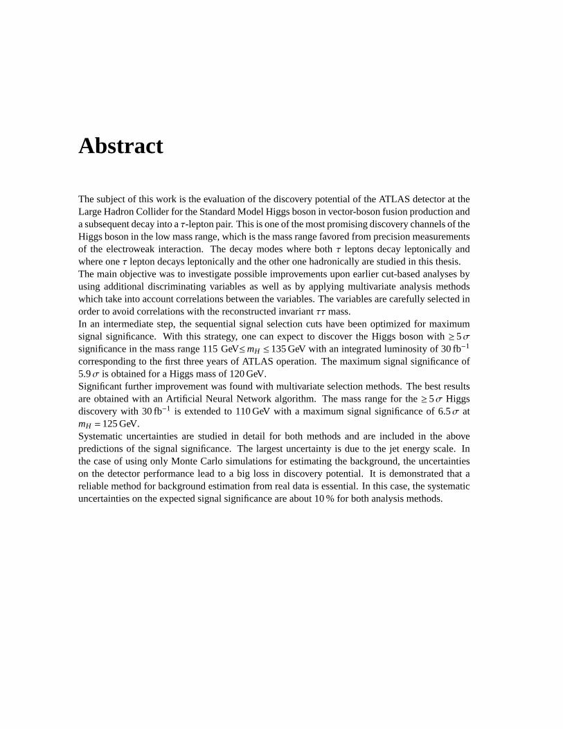
The subject of this work is the evaluation of the discovery potential of the ATLAS detector at theLarge Hadron Collider for the Standard Model Higgs boson in vector-boson fusion production anda subsequent decay into aτ-lepton pair. This is one of the most promising discovery channels of theHiggs boson in the low mass range, which is the mass range favored from precision measurementsof the electroweak interaction. The decay modes where bothτ leptons decay leptonically andwhere oneτ lepton decays leptonically and the other one hadronically are studied in this thesis.The main objective was to investigate possible improvements upon earlier cut-based analyses byusing additional discriminating variables as well as by applying multivariate analysis methodswhich take into account correlations between the variables. The variablesare carefully selected inorder to avoid correlations with the reconstructed invariantττmass.In an intermediate step, the sequential signal selection cuts have been optimized for maximumsignal significance. With this strategy, one can expect to discover the Higgs boson with≥5σsignificance in the mass range 115 GeV≤mH ≤135 GeV with an integrated luminosity of 30 fb−1
corresponding to the first three years of ATLAS operation. The maximum signal significance of5.9σ is obtained for a Higgs mass of 120 GeV.Significant further improvement was found with multivariate selection methods.The best resultsare obtained with an Artificial Neural Network algorithm. The mass range forthe≥5σ Higgsdiscovery with 30 fb−1 is extended to 110 GeV with a maximum signal significance of 6.5σ atmH =125 GeV.Systematic uncertainties are studied in detail for both methods and are includedin the abovepredictions of the signal significance. The largest uncertainty is due to thejet energy scale. Inthe case of using only Monte Carlo simulations for estimating the background, the uncertaintieson the detector performance lead to a big loss in discovery potential. It is demonstrated that areliable method for background estimation from real data is essential. In this case, the systematicuncertainties on the expected signal significance are about 10 % for bothanalysis methods.


Acknowledgements
Let me devote this page to all the people who supported my work during the lastyears.First, I want to express my gratitude to my supervisor Hubert Kroha for giving me the opportunityto do both my diploma and my PhD thesis in the MDT group at MPI. I thank him for hissupervi-sion of the thesis, for providing the means and giving me the possibility to becomepart of the teambuilding up such a fascinating experiment as the ATLAS detector, for providing me the chance toparticipate in schools, workshops, seminars and many interesting conferences.I thank Susanne Mohrdieck-Mock, Oliver Kortner, Jorg Dubbert and especially Sandra Horvatfor introducing me to the field of experimental high energy physics and guiding me through thelast years. All of them showed much patience with me and always took the time to discuss mythoughts, no matter how busy they were. Many thanks to Steffen Kaiser for his support especiallyduring the last weeks.Thank you to all the members of the MDT group for creating the stimulating and pleasant atmo-sphere, the coffee in the morning, the Cheeseburgers and Spezis, the beers, bars and Schnitzels,for the tabletennis matches and much more.
Bei all meinen Freunden bedanke ich mich fur ihre Unterstutzung, das Interesse an meiner Arbeitund deren Fortschritt sowie dafur, dass sie trotz meiner eingeschrankten Zeit uneingeschrankthinter mir gestanden haben. Fur die Hilfe beim Korrekturlesen und Ausdrucken mochte ich michaußerdem ganz herzlich bei Martin Muhlegger bedanken.Meiner Familie, speziell meinen Eltern Magdalena und Bruno Groh, gebuhrt ganz besondererDank fur den Ruckhalt, den sie mir wahrend der letzten nun schon fast 30 Jahre gegeben habenund dafur, dass sie mir mein Studium ermoglicht haben.
Unmoglich in Worte zu fassen will ich trotzdem meinen unendlichen Dank dem allerwichtigstenMenschen in meinem Leben aussprechen: meiner Irene. Trotz ihrer eigenen Arbeitsbelastung undihres Studiums hat sie mich immer in allen alltaglichen und nicht alltaglichen Dingen unterstutztund mir die Kraft und die Geborgenheit gegeben, ohne die diese Arbeit nicht moglich gewesenware. Ganz besonders danke ich ihr fur ihr Verstandnis, wenn ich aufgrund meiner zahlreichenAufenthalte am CERN oder bei Konferenzen, sowie vor allem in den letztenMonaten nur sehrwenig Zeit mit ihr verbringen konnte.

Contents
1 Introduction 1
2 Theoretical Background 32.1 The Standard Model. . . . . . . . . . . . . . . . . . . . . . . . . . . . . . . . 32.2 The Higgs Boson. . . . . . . . . . . . . . . . . . . . . . . . . . . . . . . . . . 6
2.2.1 Limits on the Higgs Boson Mass. . . . . . . . . . . . . . . . . . . . . . 62.2.2 Higgs Boson Production Mechanisms. . . . . . . . . . . . . . . . . . . 82.2.3 Higgs Boson Decay Channels. . . . . . . . . . . . . . . . . . . . . . . 8
3 The LHC and ATLAS 153.1 The Large Hadron Collider. . . . . . . . . . . . . . . . . . . . . . . . . . . . . 153.2 The ATLAS Experiment . . . . . . . . . . . . . . . . . . . . . . . . . . . . . . 17
3.2.1 Physics Goals and Detector Requirements. . . . . . . . . . . . . . . . . 173.2.2 The ATLAS Coordinate System. . . . . . . . . . . . . . . . . . . . . . 183.2.3 The ATLAS Detector. . . . . . . . . . . . . . . . . . . . . . . . . . . . 18
4 Installation and Commissioning of the ATLAS Muon Chambers 274.1 Chamber Installation. . . . . . . . . . . . . . . . . . . . . . . . . . . . . . . . 27
4.1.1 MDT Chamber Sag Adjustment. . . . . . . . . . . . . . . . . . . . . . 304.1.2 Tests After Chamber Installation. . . . . . . . . . . . . . . . . . . . . . 32
4.2 Commissioning of the Muon Spectrometer with Cosmic Muons. . . . . . . . . 324.2.1 Drift Tube Efficiency Measurement. . . . . . . . . . . . . . . . . . . . 334.2.2 Reconstruction of Cosmic Muon Tracks. . . . . . . . . . . . . . . . . . 334.2.3 Alignment with Straight Muon Tracks. . . . . . . . . . . . . . . . . . . 354.2.4 Curved Muon Tracks. . . . . . . . . . . . . . . . . . . . . . . . . . . . 36
5 The Search for the Higgs Boson 415.1 Signal and Background Processes. . . . . . . . . . . . . . . . . . . . . . . . . 41
5.1.1 Monte Carlo Simulation. . . . . . . . . . . . . . . . . . . . . . . . . . 445.1.2 Detector Simulation. . . . . . . . . . . . . . . . . . . . . . . . . . . . 50
5.2 Detector Performance. . . . . . . . . . . . . . . . . . . . . . . . . . . . . . . . 515.2.1 Trigger Efficiency. . . . . . . . . . . . . . . . . . . . . . . . . . . . . . 525.2.2 Electron Reconstruction. . . . . . . . . . . . . . . . . . . . . . . . . . 535.2.3 Muon Reconstruction. . . . . . . . . . . . . . . . . . . . . . . . . . . . 54
ix
x CONTENTS
5.2.4 Jet Reconstruction Performance. . . . . . . . . . . . . . . . . . . . . . 565.2.5 τ Jet Reconstruction Performance. . . . . . . . . . . . . . . . . . . . . 565.2.6 b Jet Identification . . . . . . . . . . . . . . . . . . . . . . . . . . . . . 605.2.7 Missing Energy Reconstruction. . . . . . . . . . . . . . . . . . . . . . 60
5.3 Reconstruction of the Higgs Mass. . . . . . . . . . . . . . . . . . . . . . . . . 635.4 Event Selection Criteria. . . . . . . . . . . . . . . . . . . . . . . . . . . . . . . 67
5.4.1 τ-Decay Products Criteria. . . . . . . . . . . . . . . . . . . . . . . . . 675.4.2 Tagging Jets Criteria. . . . . . . . . . . . . . . . . . . . . . . . . . . . 735.4.3 Overall Event Topology (Jets andτ-Decay Products) Criteria. . . . . . . 80
6 Optimization of the Signal Selection 876.1 Composition of the Background. . . . . . . . . . . . . . . . . . . . . . . . . . 876.2 Preselection. . . . . . . . . . . . . . . . . . . . . . . . . . . . . . . . . . . . . 876.3 Signal-to-Background Ratio. . . . . . . . . . . . . . . . . . . . . . . . . . . . 896.4 Treatment of Correlations. . . . . . . . . . . . . . . . . . . . . . . . . . . . . . 92
6.4.1 Parallel Cut Optimization. . . . . . . . . . . . . . . . . . . . . . . . . 926.4.2 Iterative Cut Optimization. . . . . . . . . . . . . . . . . . . . . . . . . 94
6.5 Cut Efficiency Factorization for thett Background. . . . . . . . . . . . . . . . . 956.6 Results of the Cut-Based Analysis. . . . . . . . . . . . . . . . . . . . . . . . . 100
6.6.1 Results for the Leptonic Decay Channel. . . . . . . . . . . . . . . . . . 1006.6.2 Results for the Semileptonic Decay Channel. . . . . . . . . . . . . . . . 1046.6.3 Comparison of Detailed and Fast Simulation for thett Background. . . . 109
7 Multivariate Analysis 1157.1 Motivation. . . . . . . . . . . . . . . . . . . . . . . . . . . . . . . . . . . . . . 1157.2 Overview of Multivariate Analysis Methods. . . . . . . . . . . . . . . . . . . . 117
7.2.1 Projective Likelihood Method. . . . . . . . . . . . . . . . . . . . . . . 1177.2.2 Fisher Discriminant Method. . . . . . . . . . . . . . . . . . . . . . . . 1187.2.3 Artificial Neural Networks. . . . . . . . . . . . . . . . . . . . . . . . . 1187.2.4 Boosted Decision Trees. . . . . . . . . . . . . . . . . . . . . . . . . . 1207.2.5 Decorrelation of Input Variables. . . . . . . . . . . . . . . . . . . . . . 121
7.3 Training of Multivariate Methods. . . . . . . . . . . . . . . . . . . . . . . . . . 1227.4 Selection of Input Variables. . . . . . . . . . . . . . . . . . . . . . . . . . . . . 1227.5 Performance of the Multivariate Analysis Methods. . . . . . . . . . . . . . . . 126
7.5.1 Event Selection for Performance Tests. . . . . . . . . . . . . . . . . . . 1267.5.2 Performance Criterion. . . . . . . . . . . . . . . . . . . . . . . . . . . 1267.5.3 Comparison of Multivariate Analysis Methods. . . . . . . . . . . . . . 1287.5.4 The ANN Output Distribution. . . . . . . . . . . . . . . . . . . . . . . 129
7.6 Multivariate Analysis Results. . . . . . . . . . . . . . . . . . . . . . . . . . . . 1307.6.1 The Leptonic Decay Channel. . . . . . . . . . . . . . . . . . . . . . . . 1307.6.2 The Semileptonic Decay Channel. . . . . . . . . . . . . . . . . . . . . 131
7.7 Systematic Tests. . . . . . . . . . . . . . . . . . . . . . . . . . . . . . . . . . . 1347.7.1 Separate Treatment of Backgrounds. . . . . . . . . . . . . . . . . . . . 1347.7.2 Number of Training Events. . . . . . . . . . . . . . . . . . . . . . . . . 135
CONTENTS xi
7.7.3 Sensitivity of the Training to Statistical Fluctuations. . . . . . . . . . . 1357.7.4 Influence of the Preselection. . . . . . . . . . . . . . . . . . . . . . . . 1377.7.5 Influence of the MVA Configuration. . . . . . . . . . . . . . . . . . . . 1377.7.6 Influence on themττ Distribution. . . . . . . . . . . . . . . . . . . . . . 138
8 Higgs Discovery Potential 1418.1 Signal Significance Determination. . . . . . . . . . . . . . . . . . . . . . . . . 141
8.1.1 Results without Systematic Uncertainties. . . . . . . . . . . . . . . . . 1448.2 Systematic Uncertainties. . . . . . . . . . . . . . . . . . . . . . . . . . . . . . 144
8.2.1 Theoretical Uncertainties. . . . . . . . . . . . . . . . . . . . . . . . . . 1448.2.2 Uncertainty due to the Fast Simulation for thett Background. . . . . . . 1478.2.3 Detector-Related Experimental Uncertainties. . . . . . . . . . . . . . . 1478.2.4 Impact of Systematic Uncertainties on the Expected Discovery Potential. 1528.2.5 Profile Likelihood Calculation. . . . . . . . . . . . . . . . . . . . . . . 161
9 Summary 169
A Details for all Higgs Masses 171
List of Figures 177
List of Tables 181
Bibliography 183

Chapter 1
Introduction
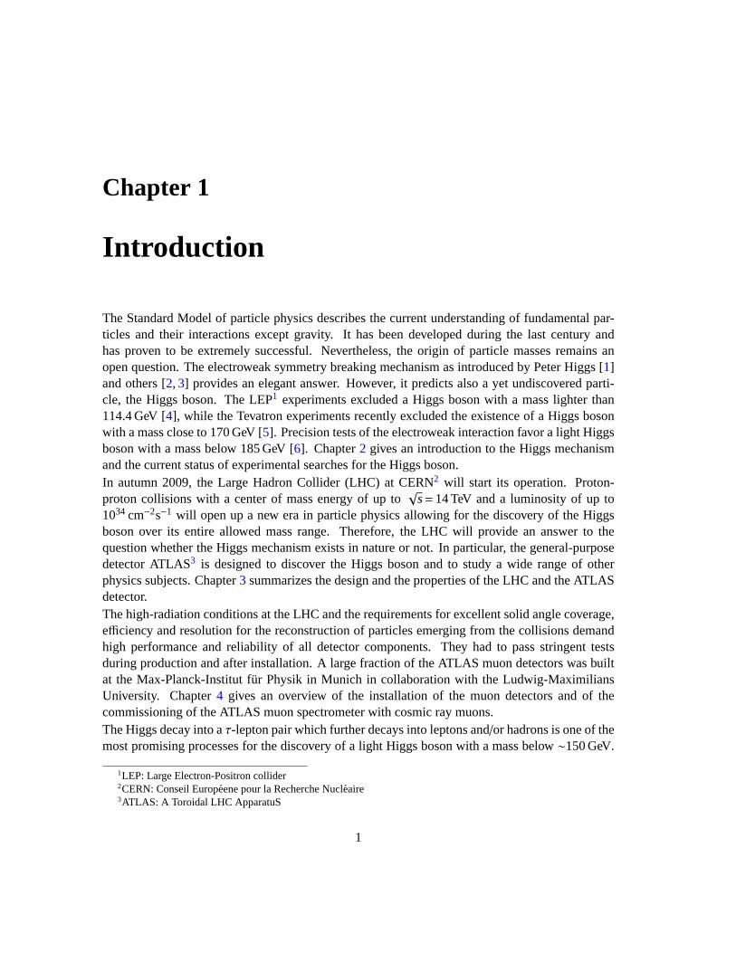
The Standard Model of particle physics describes the current understanding of fundamental par-ticles and their interactions except gravity. It has been developed duringthe last century andhas proven to be extremely successful. Nevertheless, the origin of particle masses remains anopen question. The electroweak symmetry breaking mechanism as introducedby Peter Higgs [1]and others [2,3] provides an elegant answer. However, it predicts also a yet undiscovered parti-cle, the Higgs boson. The LEP1 experiments excluded a Higgs boson with a mass lighter than114.4 GeV [4], while the Tevatron experiments recently excluded the existence of a Higgsbosonwith a mass close to 170 GeV [5]. Precision tests of the electroweak interaction favor a light Higgsboson with a mass below 185 GeV [6]. Chapter2 gives an introduction to the Higgs mechanismand the current status of experimental searches for the Higgs boson.In autumn 2009, the Large Hadron Collider (LHC) at CERN2 will start its operation. Proton-proton collisions with a center of mass energy of up to
√s=14 TeV and a luminosity of up to
1034 cm−2s−1 will open up a new era in particle physics allowing for the discovery of the Higgsboson over its entire allowed mass range. Therefore, the LHC will providean answer to thequestion whether the Higgs mechanism exists in nature or not. In particular, the general-purposedetector ATLAS3 is designed to discover the Higgs boson and to study a wide range of otherphysics subjects. Chapter3 summarizes the design and the properties of the LHC and the ATLASdetector.The high-radiation conditions at the LHC and the requirements for excellentsolid angle coverage,efficiency and resolution for the reconstruction of particles emerging from thecollisions demandhigh performance and reliability of all detector components. They had to pass stringent testsduring production and after installation. A large fraction of the ATLAS muon detectors was builtat the Max-Planck-Institut fur Physik in Munich in collaboration with the Ludwig-MaximiliansUniversity. Chapter4 gives an overview of the installation of the muon detectors and of thecommissioning of the ATLAS muon spectrometer with cosmic ray muons.The Higgs decay into aτ-lepton pair which further decays into leptons and/or hadrons is one of themost promising processes for the discovery of a light Higgs boson with a mass below∼150 GeV.
1LEP: Large Electron-Positron collider2CERN: Conseil Europeene pour la Recherche Nucleaire3ATLAS: A Toroidal LHC ApparatuS
1
2 Chapter 1. Introduction
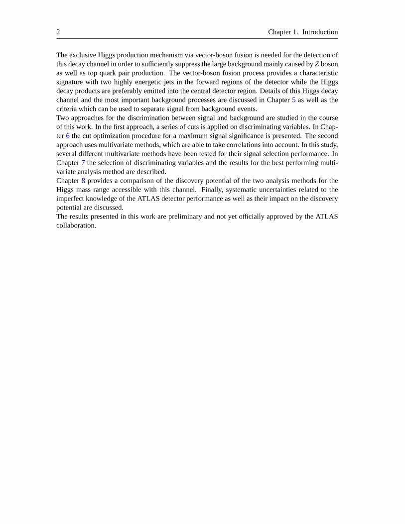
The exclusive Higgs production mechanism via vector-boson fusion is needed for the detection ofthis decay channel in order to sufficiently suppress the large background mainly caused byZ bosonas well as top quark pair production. The vector-boson fusion process provides a characteristicsignature with two highly energetic jets in the forward regions of the detector while the Higgsdecay products are preferably emitted into the central detector region. Details of this Higgs decaychannel and the most important background processes are discussedin Chapter5 as well as thecriteria which can be used to separate signal from background events.Two approaches for the discrimination between signal and background are studied in the courseof this work. In the first approach, a series of cuts is applied on discriminating variables. In Chap-ter 6 the cut optimization procedure for a maximum signal significance is presented. The secondapproach uses multivariate methods, which are able to take correlations into account. In this study,several different multivariate methods have been tested for their signal selection performance. InChapter7 the selection of discriminating variables and the results for the best performing multi-variate analysis method are described.Chapter8 provides a comparison of the discovery potential of the two analysis methodsfor theHiggs mass range accessible with this channel. Finally, systematic uncertaintiesrelated to theimperfect knowledge of the ATLAS detector performance as well as their impact on the discoverypotential are discussed.The results presented in this work are preliminary and not yet officially approved by the ATLAScollaboration.

Chapter 2
Theoretical Background
The Standard Model is an extremely successful theory comprising our current understandingof fundamental particles and their interactions. It is based on a spontaneously broken localS U(3)× S U(2)× U(1) gauge theory describing the strong, weak and electromagnetic interac-tions. A brief overview of the Standard Model is given in Section2.1 including the Higgs mech-anism which describes the origin of the masses of the fundamental particles.Further details canbe found, for example, in [7]. Section2.2 deals with the Higgs boson predicted by the theory.Limits on the Higgs boson mass from theory and experiments are discussed in Section2.2.1. InSections2.2.2and2.2.3, the production mechanisms and decay channels of the Higgs boson inthe Standard Model are described.
2.1 The Standard Model
In the Standard Model, three types of fundamental particles are distinguished according to theirspin:
• Fermions with spin 1/2The Fermionsf are the matter constituents and are grouped further into leptonsl and quarksq. Both leptons and quarks exist in three generations with increasing mass. All known stablematter on earth is formed of fermions of the first generation. Table2.1gives an overview ofthe known fermions.
• Bosons with spin 1They are the vector bosons of the gauge fields mediating the three fundamental forces: theelectromagnetic, the weak and the strong interaction.
• The Higgs boson with spin 0 is associated with the spontaneous breaking of the electroweakgauge symmetry.
All three forces are described by local gauge theories with the three simplest gauge symmetrygroupsU(1), S U(2) andS U(3). The strong force between the quarks is described by QuantumChromodynamics (QCD) [8,9,10,11], a S U(3) gauge theory. It contains eight gauge fields asso-ciated with eight massless vector bosons called gluons.
3
4 Chapter 2. Theoretical Background
Generation ElectricCharge
1 2 3 [e]
Leptonsνe
eνµ
µ
ντ
τ
0−1
Quarksud
cs
tb
+2/3−1/3
Table 2.1: The three generations of fermions in the Standard Model.
Between 1960 and 1968, Glashow [12], Weinberg [13] and Salam [14] developed aS U(2)× U(1)gauge field theory which combines the electromagnetic and weak force and isthus called elec-troweak theory. TheGlashow-Salam-Weinberg Theoryincludes the localS U(2) gauge group ofthe weak isospin and theU(1) gauge group of the weak hypercharge with two gauge couplingsg andg′ respectively. TheS U(2) gauge symmetry requires three gauge fieldsW1
µ ,W2µ andW3
µ
related to the three componentsJi(i = 1,2,3) of the weak isospin vector, while theU(1) gaugetheory contains only one gauge fieldBµ related to the weak hypercharge. Linear combinations ofthese four gauge fields describe the observed particles mediating the weakand electromagneticinteractions, namely the charged weak gauge bosonsW+ andW− described by the fields
W±µ =1√
2(W1µ ± iW2
µ) (2.1)
and the neutral weak and electromagnetic gauge fields
( AµZµ
)
=
( cosθW sinθWsinθW cosθW
)( BµW3µ
)
(2.2)
which correspond to the photon and theZ0 boson and are related toBµ andW3µ by a rotation with
the weak mixing or Weinberg angleθW.However, this theory has one severe problem: To conserveS U(2) symmetry, the weak gaugebosonsW± andZ0 have to be massless which is in contradiction to observations.
The Higgs Mechanism The solution to the problem of massive gauge bosons was provided byP. W. Higgs [1] and others [15,16] in the year 1964. Based on the work of Nambu [2] and Gold-stone [3], they developed a mechanism, the Higgs mechanism, in which massive gauge bosons canbe accommodated by introducing a complex scalar field of the form
φ =
(
φ+
φ0
)
(2.3)
described by the LagrangianL = Dµφ
†Dµφ − V (2.4)
2.1. The Standard Model 5
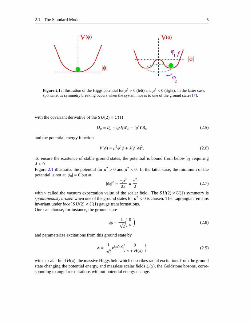
Figure 2.1: Illustration of the Higgs potential forµ2 > 0 (left) andµ2 < 0 (right). In the latter case,spontaneous symmetry breaking occurs when the system movesto one of the ground states [7].
with the covariant derivative of theS U(2)× U(1)
Dµ = ∂µ − igJiWµi − ig′YBµ (2.5)
and the potential energy function
V(φ) = µ2φ†φ + λ(φ†φ)2. (2.6)
To ensure the existence of stable ground states, the potential is bound from below by requiringλ > 0.Figure2.1 illustrates the potential forµ2 > 0 andµ2 < 0. In the latter case, the minimum of thepotential is not at|φ0| = 0 but at:
|φ0|2 =−µ2
2λ≡ v2
2(2.7)
with v called the vacuum expectation value of the scalar field. TheS U(2)× U(1) symmetry isspontaneously brokenwhen one of the ground states forµ2 < 0 is chosen. The Lagrangian remainsinvariant underlocal S U(2)× U(1) gauge transformations.One can choose, for instance, the ground state
φ0 =1√
2
( 0v
)
(2.8)
and parameterize excitations from this ground state by
φ =1√
2ei j iζi (x)
( 0v+ H(x)
)
(2.9)
with a scalar fieldH(x), the massive Higgs field which describes radial excitations from the groundstate changing the potential energy, and massless scalar fieldsζi(x), the Goldstone bosons, corre-sponding to angular excitations without potential energy change.
6 Chapter 2. Theoretical Background
The latter can be eliminated by a localS U(2) gauge transformation leading to the parameterizationof the scalar field
φ =1√
2
( 0v+ H
)
. (2.10)
Introducing the ansatz2.10 into the Lagrangian2.4 of the electroweak theory and using equa-tions2.1and2.2, one obtains the following expressions from the kinetic terms:
g2v2
8W+µW+µ +
g2v2
8W−µW−µ +
g2v2
8 cos2θWZµZ
µ. (2.11)
These terms can be identified as mass terms of theW± andZ0 bosons which thus acquire masses
mZ cosθW = mW =vg2
(2.12)
due to the coupling to the Higgs field.The masses of the fermions are also generated by spontaneousS U(2)× U(1) breaking due toYukawa couplings to the Higgs field. The coupling strength of a fermion to the Higgs field, whichis not predicted by the theory, is proportional to the fermion mass.The Glashow-Salam-Weinberg theory includes the Higgs mechanism. It predicts theW andZboson and their properties, like mass and decay width. In 1983, the three weak gauge bosons havebeen discovered by the UA1 and UA2 experiments at CERN [17, 18, 19, 20] with the predictedproperties.
2.2 The Higgs Boson
Although the Standard Model is widely accepted and very successful in describing the phenomenaof particle physics, there is still one part missing: The experimental verification of the existenceof the Higgs boson introduced in equation2.8. The value of the mass of the Higgs boson
mH =√
2λ v (2.13)
is not predicted by the Standard Model and has to be measured. Howeverthe possible mass rangeis restricted by theoretical and experimental constraints. These limits are briefly discussed in thefollowing.
2.2.1 Limits on the Higgs Boson Mass
Theoretical Limits Several consistency requirements of the theory set upper and lower boundson the Higgs mass in the Standard Model depending on the energy scaleΛ up to which the Stan-dard Model is valid and no new interactions or particles appear. Values ofΛ up to the PlanckMassMPlanck= 1019 GeV are considered above which gravitation becomes as strong as the otherfundamental forces and the Standard Model must, at the latest, be extended by a quantum theoryof gravitation. Here, only the results are summarized (further details can befound, for example,in [21] and references therein):
2.2. The Higgs Boson 7
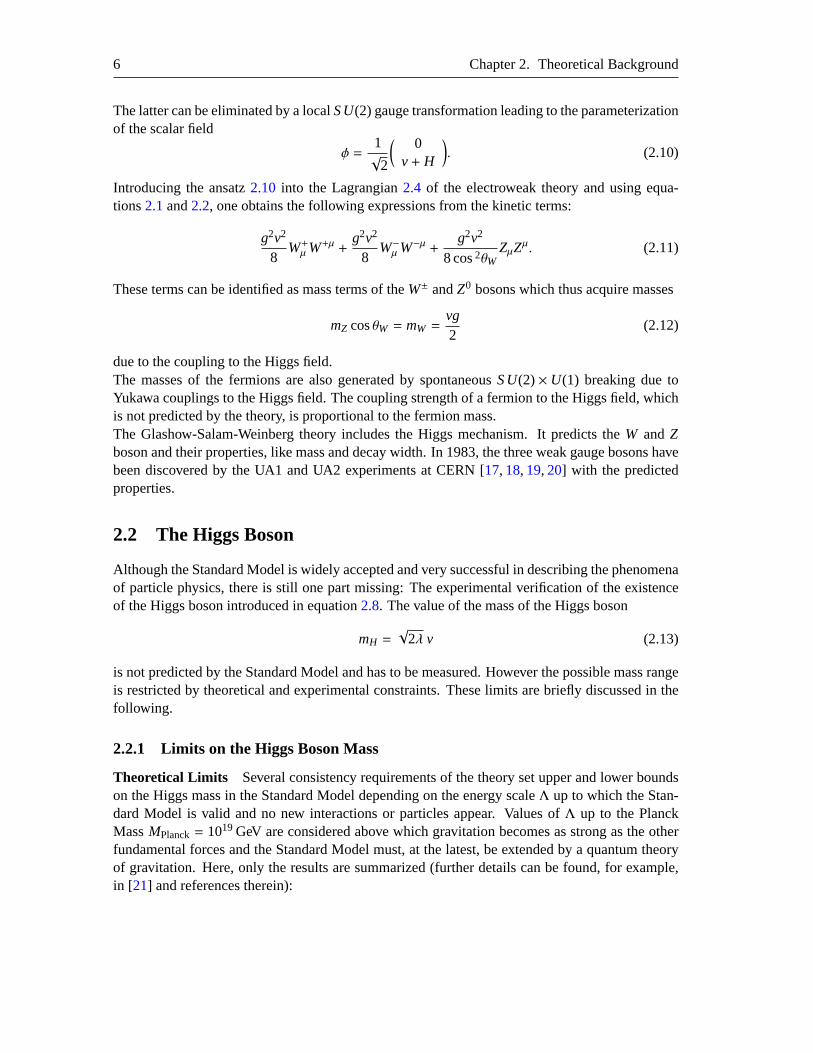
Figure 2.2: Upper and lower theoretical bounds on the Higgs boson mass asa function of the energyscaleΛ up to which the Standard Model is valid. A top quark mass ofmt = 175 GeV is assumed.The bands indicate the theoretical uncertainties. [21]
• Unitarity of the electroweak interactions, in particular of theW+W− →W+W− scatteringamplitude, limits the Higgs boson mass tomH . 1 TeV.
• The requirement of finite self-coupling of Higgs bosons, including Higgs and top quarkloops, restricts the Higgs mass with an upper bound depending onΛ:mH . 600 GeV forΛ = 1 TeV andmH . 180 GeV forΛ = MPlanck.
• To ensure the stability of the Higgs ground state, the Higgs potential (see equation2.6) hasto have a lower bound (λ(Λ) > 0). This results in a lower limit on the Higgs boson mass ofmH & 55 GeV forΛ = 1 TeV andmH & 130 GeV forΛ = MPlanck.
Figure2.2shows the theoretical upper and lower bounds for the Standard Model Higgs boson as afunction ofΛ. The measurement of the Higgs boson mass will constrainΛ. For example, a Higgsboson mass ofmH = 500 GeV implies that the Standard Model breaks down already at a muchlower energy scale thanMPlanck.
ForΛ = 1 TeV, theory predicts a Higgs boson in the wide mass range of
55 GeV. mH . 600 GeV. (2.14)
Limits from Experiments A lower bound of the Higgs boson mass comes from direct Higgsboson searches at the Large Electron Positron Collider LEP at CERN. Bycombining the data of
8 Chapter 2. Theoretical Background
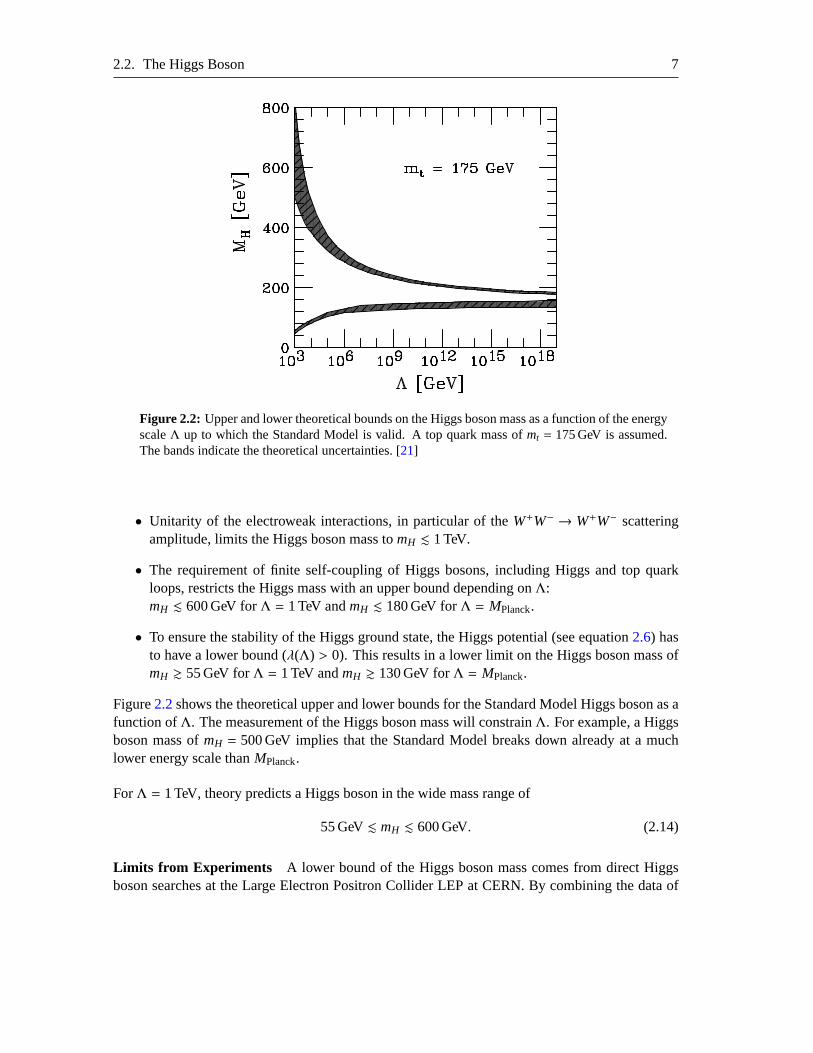
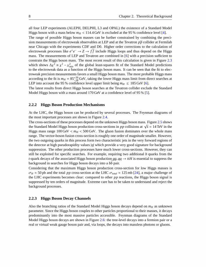
all four LEP experiments (ALEPH, DELPHI, L3 and OPAL) the existence of a Standard ModelHiggs boson with a mass belowmH < 114.4 GeV is excluded at the 95 % confidence level [4].The range of possible Higgs boson masses can be further constrained by combining the preci-sion measurements of electroweak observables at LEP and at the Tevatron pp collider at Fermilabnear Chicago with the experiments CDF and D0. Higher order corrections tothe calculation ofelectroweak processes likee+e− → Z→ f f include Higgs loops and thus depend on the Higgsmass. The measurements of LEP and Tevatron are combined in [6] with a precision sufficient toconstrain the Higgs boson mass. The most recent result of this calculation isgiven in Figure2.3which shows∆χ2 ≡ χ2 − χ2
min of the global least-squares fit of the Standard Model predictionsto the electroweak data as a function of the Higgs boson mass. It can be seen that the fit to elec-troweak precision measurements favors a small Higgs boson mass. The most probable Higgs massaccording to the fit ismH = 85+39
−28 GeV, taking the lower Higgs mass limit from direct searches atLEP into account the 95 % confidence level upper limit beingmH ≤ 185 GeV [6].The latest results from direct Higgs boson searches at the Tevatron collider exclude the StandardModel Higgs boson with a mass around 170 GeV at a confidence level of 95 % [5].
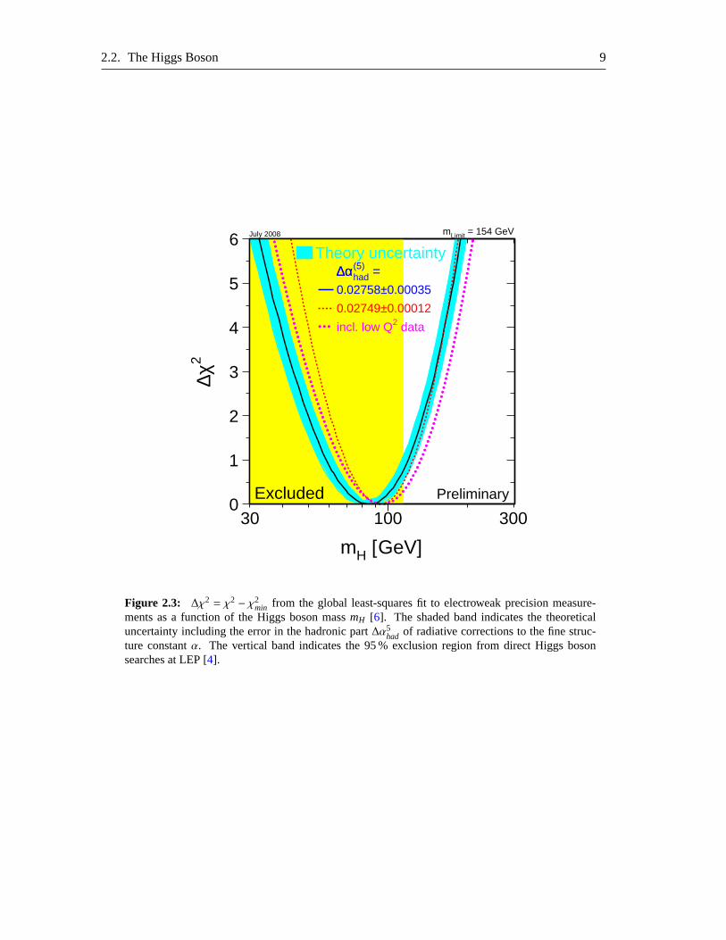
2.2.2 Higgs Boson Production Mechanisms
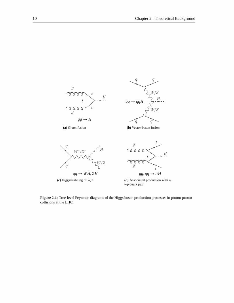
At the LHC, the Higgs boson can be produced by several processes.The Feynman diagrams ofthe most important processes are shown in Figure2.4.The cross-sections of these processes depend on the unknown Higgsboson mass. Figure2.5showsthe Standard Model Higgs boson production cross-sections inppcollisions at
√s= 14 TeV in the
Higgs mass range 100 GeV< mH < 500 GeV. The gluon fusion dominates over the whole massrange. The vector-boson fusion cross-section is roughly one orderof magnitude smaller. However,the two outgoing quarks in this process form two characteristic jets in the veryforward regions ofthe detector at high pseudorapidity values|η| which provide a very good signature for backgroundsuppression. The other production processes have much lower cross-sections. However, they canstill be exploited for specific searches. For example, requiring two additional b quarks from thet-quark decays of the associated Higgs boson productiongg,qq→ ttH is essential to suppress thebackground in searches for Higgs boson decays into abb pair.Considering that the maximum Higgs boson production cross-section for lowHiggs masses isσH ≈ 50 pb and the totalpp cross-section at the LHCσtotal ≈ 125 mb [24], a major challenge ofthe LHC experiments becomes clear: compared to otherpp reactions, the Higgs boson signal issuppressed by ten orders of magnitude. Extreme care has to be taken to understand and reject thebackground processes.
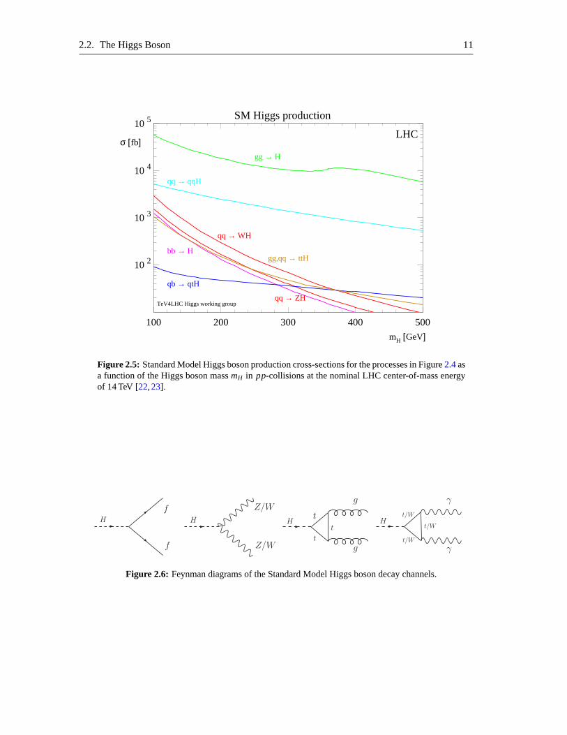
2.2.3 Higgs Boson Decay Channels
Also the branching ratios of the Standard Model Higgs boson decays depend onmH as unknownparameter. Since the Higgs boson couples to other particles proportional totheir masses, it decayspredominantly into the most massive particles accessible. Feynman diagrams ofthe StandardModel Higgs boson decays are shown in Figure2.6: the tree-level decays into a fermion pair or areal or virtual weak gauge boson pair and, via loops, the decays into massless photons or gluons.
2.2. The Higgs Boson 9
0
1
2
3
4
5
6
10030 300
mH [GeV]
∆χ2
Excluded Preliminary
∆αhad =∆α(5)
0.02758±0.00035
0.02749±0.00012
incl. low Q2 data
Theory uncertaintyJuly 2008 mLimit = 154 GeV
Figure 2.3: ∆χ2 = χ2 − χ2min from the global least-squares fit to electroweak precision measure-
ments as a function of the Higgs boson massmH [6]. The shaded band indicates the theoreticaluncertainty including the error in the hadronic part∆α5
had of radiative corrections to the fine struc-ture constantα. The vertical band indicates the 95 % exclusion region from direct Higgs bosonsearches at LEP [4].
10 Chapter 2. Theoretical Background
g
H
g
t
t
t
gg→ H
(a) Gluon fusion
H
q q
q q
W/Z
W/Z
qq→ qqH
(b) Vector-boson fusion
q
qW/Z
W ∗/Z∗ H
qq→WH,ZH
(c) Higgsstrahlung ofW/Z
g
g
tH
t
t
gg,qq→ ttH
(d) Associated production with atop quark pair
Figure 2.4: Tree-level Feynman diagrams of the Higgs boson production processes in proton-protoncollisions at the LHC.
2.2. The Higgs Boson 11
10 2
10 3
10 4
10 5
100 200 300 400 500
qq → WH
qq → ZH
gg → H
bb → H
qb → qtH
gg,qq → ttH
qq → qqH
mH [GeV]
σ [fb]
SM Higgs production
LHC
TeV4LHC Higgs working group
Figure 2.5: Standard Model Higgs boson production cross-sections for the processes in Figure2.4asa function of the Higgs boson massmH in pp-collisions at the nominal LHC center-of-mass energyof 14 TeV [22,23].
H
f
fH
Z/W
Z/W
H
t
t
t
g
g
Ht/W
γ
γ
t/W
t/W
Figure 2.6: Feynman diagrams of the Standard Model Higgs boson decay channels.
12 Chapter 2. Theoretical Background
mH
[GeV]
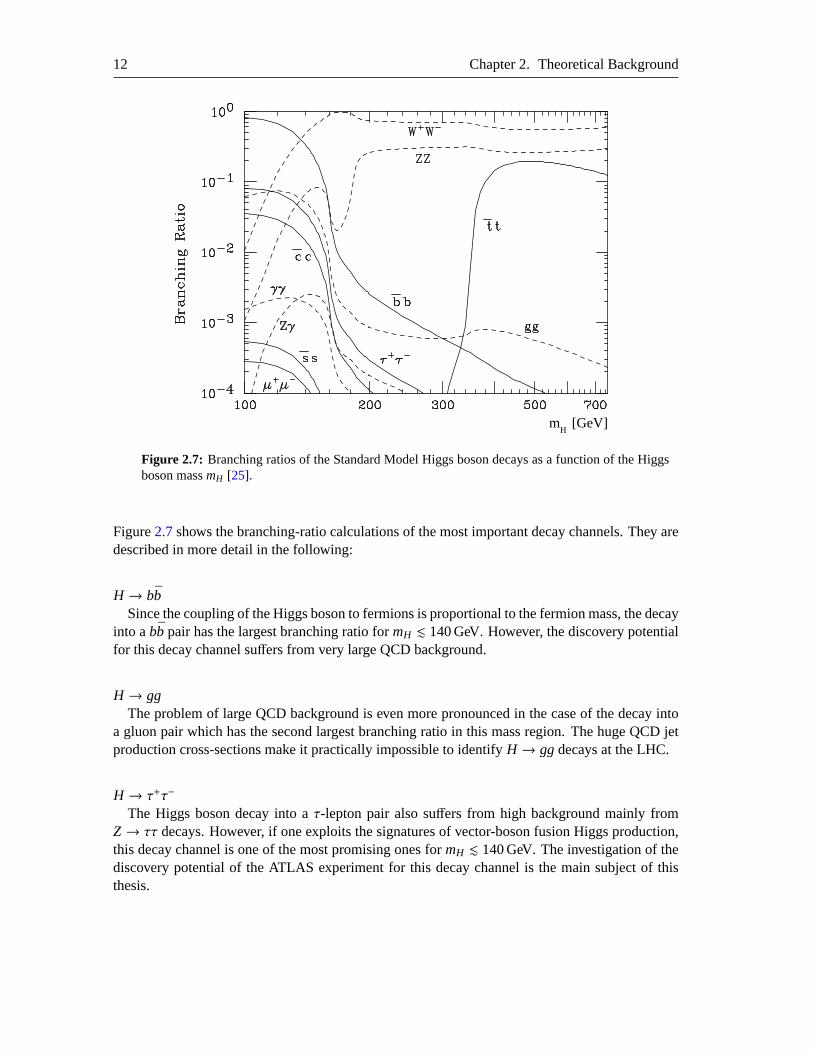
Figure 2.7: Branching ratios of the Standard Model Higgs boson decays asa function of the Higgsboson massmH [25].
Figure2.7shows the branching-ratio calculations of the most important decay channels. They aredescribed in more detail in the following:
H → bbSince the coupling of the Higgs boson to fermions is proportional to the fermionmass, the decay
into abb pair has the largest branching ratio formH . 140 GeV. However, the discovery potentialfor this decay channel suffers from very large QCD background.
H → ggThe problem of large QCD background is even more pronounced in the case of the decay into
a gluon pair which has the second largest branching ratio in this mass region. The huge QCD jetproduction cross-sections make it practically impossible to identifyH → ggdecays at the LHC.
H → τ+τ−The Higgs boson decay into aτ-lepton pair also suffers from high background mainly from
Z→ ττ decays. However, if one exploits the signatures of vector-boson fusion Higgs production,this decay channel is one of the most promising ones formH . 140 GeV. The investigation of thediscovery potential of the ATLAS experiment for this decay channel is themain subject of thisthesis.

2.2. The Higgs Boson 13
H → γγAnother important decay channel for low Higgs masses is the decayH → γγ. Although it has
only a very small branching ratio, its discovery potential is high due to the clean signature of twoenergetic photons and the high Higgs mass resolution in this channel.
H →W+W−
The branching ratio ofH →W+W− rises towards the threshold for realW-pair production. FormH ∼ 160− 180 GeV, the Higgs boson almost exclusively decays intoW+W−. Unfortunately, thebest identifiable leptonic decays ofW bosons involve neutrinos, making it impossible to accuratelyreconstruct the Higgs boson mass.
H → ZZAbove mH & 190 GeV, the decayH → ZZ is the most promising Higgs discovery channel at
LHC. The further decay of theZ bosons into electron or muon pairs provides the cleanest signatureand an excellent Higgs mass resolution. Therefore, the decayH → ZZ→ 4ℓ is known as the gold-plated discovery channel for the Higgs boson.
H → ttTheH → tt decay becomes kinematically possible abovemH & 350 GeV. However, due to the
high background rate in this decay channel and the branching ratio beingabout ten times smallerthan forH →W+W−, the decayH → tt is not a Higgs boson discovery channel at LHC.

Chapter 3
The LHC and ATLAS
Up to now, the existence of a Higgs boson has not been proven or excluded by any experiment.After more than 15 years of design and construction, a new proton-proton accelerator, the LargeHadron Collider (LHC) is put into operation at the European particle-physics laboratory CERNwhich will extend the accessible energy range up to
√s= 14 TeV at high luminosity. With this ac-
celerator it will be possible to answer the question whether the Standard Model Higgs boson existsand whether there are new phenomena beyond the Standard Model at theTeV scale. One of thegeneral-purpose experiments at the LHC is the ATLAS detector. Simulations of the performanceof the ATLAS detector are used in this work to study the discovery potential for the Higgs boson.In the following, the LHC and ATLAS are briefly introduced.
3.1 The Large Hadron Collider
The Large Hadron Collider (LHC) at CERN is a storage ring and accelerator which is equippedwith superconducting dipole magnets and which will collide two proton beams with 7TeV energyeach [26]. It is installed in a tunnel of 26.7 km circumference which housed the Large Electron-Positron collider LEP until the year 2002. The tunnel is located 50 to 175 m underground, at theborder between Switzerland and France near Geneva. The accelerator contains two vacuum beampipes, one for each beam direction, which will guide∼ 2800 bunches of up to 1011 protons each.With a diameter of 16.6µm the beams collide at four interaction points at a rate of 40 MHz. Theevent rate of app interaction process is given by:
dNdt= L · σ(
√s)
whereσ is the cross-section of the process depending on the proton-proton center-of-mass en-ergy
√s andL is the instantaneous luminosity which depends only on the beam parameters. The
design luminosity of the LHC is 1034 cm−2s−1. The expected integrated luminosity after the firstthree years of operation at lower instantaneous luminosity of 1033 cm−2s−1 is 30 fb−1. This is theintegrated luminosity for which the Higgs boson discovery potential is estimated inthis work.On average, 23 inelasticpp collisions will take place in every bunch collision. This means thateach interesting event will be overlaid with products from about 22 additional pp interactions in
15
16 Chapter 3. The LHC and ATLAS
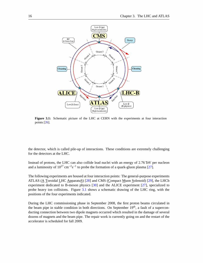
Figure 3.1: Schematic picture of the LHC at CERN with the experiments at four interactionpoints [26].
the detector, which is called pile-up of interactions. These conditions are extremely challengingfor the detectors at the LHC.
Instead of protons, the LHC can also collide lead nuclei with an energy of 2.76 TeV per nucleonand a luminosity of 1027 cm−2s−1 to probe the formation of a quark-gluon plasma [27].
The following experiments are housed at four interaction points: The general-purpose experimentsATLAS (A Toroidal LHC ApparatuS) [28] and CMS (Compact Muon Solenoid) [29], the LHCbexperiment dedicated to B-meson physics [30] and the ALICE experiment [27], specialized toprobe heavy ion collisions. Figure3.1 shows a schematic drawing of the LHC ring, with thepositions of the four experiments indicated.
During the LHC commissioning phase in September 2008, the first proton beamscirculated inthe beam pipe in stable condition in both directions. On September 19th, a fault of a supercon-ducting connection between two dipole magnets occurred which resulted in thedamage of severaldozens of magnets and the beam pipe. The repair work is currently going on and the restart of theaccelerator is scheduled for fall 2009.

3.2. The ATLAS Experiment 17
3.2 The ATLAS Experiment
ATLAS is an acronym for AToroidal LHC ApparatuSwhich refers to the configuration of themagnetic field of the outermost detector part, the muon spectrometer. Figure3.2 shows a sketchof the ATLAS detector.
3.2.1 Physics Goals and Detector Requirements
The ATLAS experiment aims to study a broad spectrum of physics topics:
• Top quark physicsSince the LHC will produce dozens of top quarks per second, precisionmeasurements oftheir production cross-section, mass, coupling and spin can be performed.
• Higgs boson physicsSearches for Higgs bosons associated with electroweak symmetry breaking in the StandardModel will be performed over the whole allowed mass range up to 1 TeV. Depending onthe production and decay mode, this requires efficient identification and precise momentummeasurement of electrons and muons, a hermetic detector for missing energymeasurement,identification ofb andτ jets and measurement of jets in the very forward region. The Higgsboson searches are the benchmark for the detector design and performance.
• Supersymmetric particlesMany supersymmetric extensions of the Standard Model predict a lightest stable supersym-metric particle that interacts only weakly and therefore escapes the detectorleading to asubstantial amount of missing energy which has to be reliably reconstructed.
• New physics searchesThe LHC opens up a completely new energy regime. Searches for any kindof new particlesor physics processes will be performed with the ATLAS experiment, including searches fornew heavy gauge bosonsW′ andZ′ with masses up to∼6 TeV, production of mini black-holes and rare decays of heavy quarks and leptons.
The studies put stringent requirements on the detector performance:
• Fast and radiation-hard detectors and readout electronics which can cope with the high ra-diation level at the LHC and are able to distinguish the decay products of 109 proton-protoninteractions per second at design luminosity.
• Hermetic detector coverage of the solid angle around the interaction region up to the veryforward regions in order to measure the decay products and the energyreleased in the colli-sions as completely as possible.
• High momentum resolution and reconstruction efficiency of charged particles, in particularelectrons and muons.
• Precise tracking of charged particles to reconstruct the decay verticesof unstable particles.

18 Chapter 3. The LHC and ATLAS
• An electromagnetic calorimeter with a very good energy and spatial resolutionto efficientlyidentify electrons and photons and to accurately measure their energy.
• A hermetic hadron calorimeter to reliably measure jet energies and the missing transverseenergy.
• A highly efficient trigger system which allows for the detection of processes even with verysmall cross-sections and which provides strong background rejection at the high event rateof the LHC.
3.2.2 The ATLAS Coordinate System
The global right-handed coordinate system of ATLAS is defined as follows:
• The origin is the nominal interaction point.
• The positive x-direction points towards the center of the LHC ring.
• The positive y-direction points upwards.
• The z-direction points along the beam line.
The azimuthal and polar angles with respect to the beam axis are denoted byφ andθ. A commonlyused quantity in collider experiments is the pseudorapidityη which is defined by
η = − ln tan(θ/2).
Distances in theη-φ-space are usually given by
∆R=√
∆η2 + ∆φ2.
Important observables are defined in the transverse x-y plane: the transverse momentumpT, thetransverse energyET and the missing transverse energyEmiss
T . The advantage of these quantities isthat they are invariant under boosts along the beam line which usually are present in hadron-hadroncollisions.
3.2.3 The ATLAS Detector
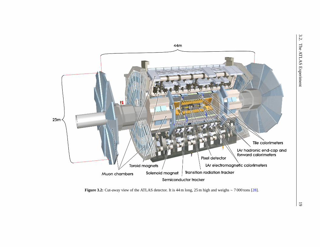
Figure3.2shows a cut-away view of the ATLAS detector. Like all typical collider experiments, itconsists of three concentric layers of subdetectors enclosing the interaction point. The innermostpart is the tracking detector, followed by the calorimeters which finally are surrounded by themuon spectrometer. The backbone of the detector is a huge superconducting magnet system. Thevarious detector elements are described in the following.
3.2.T
heAT
LAS
Experim
ent19
Figure 3.2: Cut-away view of the ATLAS detector. It is 44 m long, 25 m high and weighs∼ 7 000 tons [28].

20 Chapter 3. The LHC and ATLAS
Figure 3.3: Sketch of the ATLAS magnet system with the central solenoid coil (cylinder) and thethree toroid magnets around it [28].
The Magnet System
In order to measure the momentum of charged particles, two superconducting magnet systemsprovide a solenoidal and a toroidal magnetic field in the ATLAS detector. A sketch of the ATLASmagnet system is shown in Figure3.3.The central solenoid coil encloses the inner detector and provides a homogeneous magnetic fieldof 2 T pointing parallel to the beam line. The coil has a diameter of 2.6 m and a length of 5.8 m.In order to minimize the amount of material in front of the calorimeter, the centralsolenoid sharesone vacuum vessel with the central electromagnetic liquid-argon calorimeter. The iron absorberof the electromagnetic calorimeter serves as return yoke.For the muon spectrometer, a toroidal field configuration has been chosenwhich is divided intothree toroid magnets consisting of eight coils each: The central (barrel) toroid and two end-captoroids covering the forward regions of the detector. With a length of 25 m and an outer diameterof 20 m, the barrel toroid is the largest component of the ATLAS detector. While each coil of thebarrel toroid is housed in its own vacuum vessel, the eight coils of the end-cap toroids are containedin a common cryostat. The magnetic field provided by the toroid magnets is not uniform. The fieldstrength varies between 0.2 T and 2.5 T in the barrel region and from 0.2 T to3.5 T in the end-caps,depending on the radial distance to the beam line and the azimuthal angle.
The Inner Detector
The inner detector is designed to accurately reconstruct the trajectories of charged particles. Italso measures their point of origin (production vertex) to distinguish between particles from theprimary hard interaction, from secondary decays, or from additional pile-up interactions. Sincethe inner detector is immersed in the magnetic field of the central solenoid, the tracks of chargedparticles are bent in the transverse plane allowing for measuring particle momenta from the trackcurvature. A radiation hard, fast and highly granular detector is needed to cope with the high track
3.2. The ATLAS Experiment 21
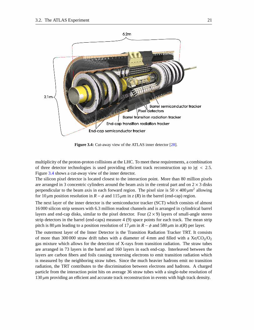
Figure 3.4: Cut-away view of the ATLAS inner detector [28].
multiplicity of the proton-proton collisions at the LHC. To meet these requirements, a combinationof three detector technologies is used providing efficient track reconstruction up to|η| < 2.5.Figure3.4shows a cut-away view of the inner detector.The silicon pixel detector is located closest to the interaction point. More than 80 million pixelsare arranged in 3 concentric cylinders around the beam axis in the central part and on 2× 3 disksperpendicular to the beam axis in each forward region. The pixel size is 50 × 400µm2 allowingfor 10µm position resolution inR− φ and 115µm in z (R) in the barrel (end-cap) region.
The next layer of the inner detector is the semiconductor tracker (SCT) which consists of almost16 000 silicon strip sensors with 6.3 million readout channels and is arrangedin cylindrical barrellayers and end-cap disks, similar to the pixel detector. Four (2× 9) layers of small-angle stereostrip detectors in the barrel (end-caps) measure 4 (9) space points foreach track. The mean strippitch is 80µm leading to a position resolution of 17µm in R− φ and 580µm in z(R) per layer.
The outermost layer of the Inner Detector is the Transition Radiation Tracker TRT. It consistsof more than 300 000 straw drift tubes with a diameter of 4 mm and filled with a Xe/CO2/O2
gas mixture which allows for the detection of X-rays from transition radiation.The straw tubesare arranged in 73 layers in the barrel and 160 layers in each end-cap. Interleaved between thelayers are carbon fibers and foils causing traversing electrons to emit transition radiation whichis measured by the neighboring straw tubes. Since the much heavier hadrons emit no transitionradiation, the TRT contributes to the discrimination between electrons and hadrons. A chargedparticle from the interaction point hits on average 36 straw tubes with a single-tube resolution of130µm providing an efficient and accurate track reconstruction in events with high track density.
22 Chapter 3. The LHC and ATLAS
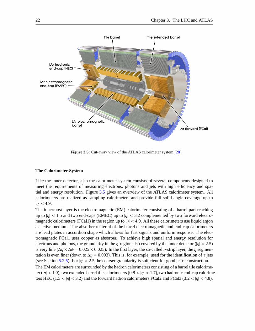
Figure 3.5: Cut-away view of the ATLAS calorimeter system [28].
The Calorimeter System
Like the inner detector, also the calorimeter system consists of several components designed tomeet the requirements of measuring electrons, photons and jets with high efficiency and spa-tial and energy resolution. Figure3.5 gives an overview of the ATLAS calorimeter system. Allcalorimeters are realized as sampling calorimeters and provide full solid anglecoverage up to|η| < 4.9.The innermost layer is the electromagnetic (EM) calorimeter consisting of a barrel part reachingup to |η| < 1.5 and two end-caps (EMEC) up to|η| < 3.2 complemented by two forward electro-magnetic calorimeters (FCal1) in the region up to|η| < 4.9. All these calorimeters use liquid argonas active medium. The absorber material of the barrel electromagnetic and end-cap calorimetersare lead plates in accordion shape which allows for fast signals and uniform response. The elec-tromagnetic FCal1 uses copper as absorber. To achieve high spatial andenergy resolution forelectrons and photons, the granularity in theη-region also covered by the inner detector (|η| < 2.5)is very fine (∆η × ∆φ = 0.025× 0.025). In the first layer, the so-calledη-strip layer, theη segmen-tation is even finer (down to∆η = 0.003). This is, for example, used for the identification ofτ jets(see Section5.2.5). For |η| > 2.5 the coarser granularity is sufficient for good jet reconstruction.The EM calorimeters are surrounded by the hadron calorimeters consistingof a barrel tile calorime-ter (|η| < 1.0), two extended barrel tile calorimeters (0.8 < |η| < 1.7), two hadronic end-cap calorime-ters HEC (1.5 < |η| < 3.2) and the forward hadron calorimeters FCal2 and FCal3 (3.2 < |η| < 4.8).

3.2. The ATLAS Experiment 23
The tile calorimeters use plastic scintillator as active material and steel as absorber material ar-ranged in three layers with a granularity of∆η × ∆φ = 0.1× 0.1. The HEC calorimeters use liquidargon as active material and copper as absorber material with a granularity of ∆η × ∆φ = 0.1× 0.1for |η| < 2.5 and∆η × ∆φ = 0.2× 0.2 for |η| > 2.5. The FCal2 and FCal3 have a readout cell size of∆x× ∆y=3.3× 4.2 cm2 and∆x× ∆y = 5.4× 4.7 cm2 respectively. Both use liquid argon as activeand tungsten as absorber material. The latter has a shorter interaction lengthas copper.The total thickness of the calorimeter system is more than 22 radiation lengths (X0) and aboutten hadronic interaction lengths. This ensures a good energy resolution of highly energetic jets,precise reconstruction of missing energy and minimizes punch-through of particles to the muonspectrometer. The total number of readout channels of the ATLAS calorimeter system is∼260 000.
The Muon Spectrometer
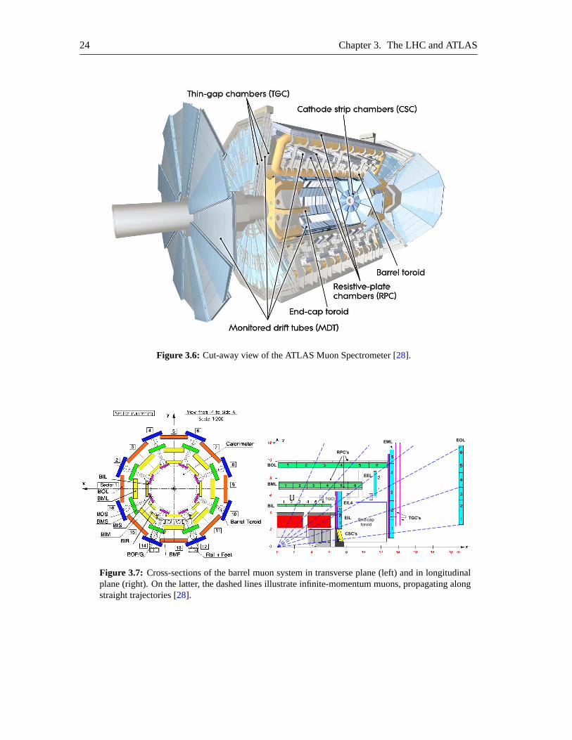
Figures3.6 and3.7 show the layout of the muon spectrometer. The outer dimensions of 44 mlength and 25 m diameter make the ATLAS detector the largest detector ever built for a colliderexperiment. Three layers of muon detectors arranged in horizontal concentric cylinders in thebarrel region and in vertical discs in the two end-caps measure the deflection of the muon tracksdue to the magnetic field provided by the three toroid magnets.The bending power
∫
Bdl along the tracks ranges from 1.5 to 5.5 Tm in the barrel part and from1 to 7.5 Tm in the end-cap regions. To minimize multiple scattering, the magnetic field ofthemuon spectrometer is generated in air (air-core toroid magnets) and the support structure is madeof aluminum.To accurately measure muon tracks and provide a muon trigger, the muon spectrometer is instru-mented with four detector types:
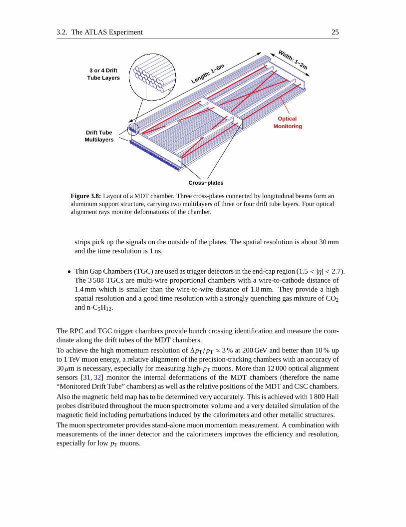
• Monitored Drift Tube chambers (MDT) are the precision muon tracking detectors over mostof the muon spectrometer acceptance. 1 150 chambers contain in total 354 000 drift tubescovering an active area of 5 500 m2. Each chamber consists of two multilayers of three orfour tube layers that are glued on the cross-plates of an aluminum support structure as shownin Figure3.8. The aluminum tubes of 30 mm diameter and 400µm wall thickness are filledwith an Ar(93%)CO2(7%) gas mixture at a pressure of 3 bar. The gold-plated tungsten-rhenium anode wires in the tube centers are positioned with respect to the chambers with anaccuracy of 20µm. At a high voltage of 3 080 V, the maximum drift time is about 700 ns.The average spatial resolution of a drift tube is 80µm. The track position resolution of theMDT chambers is 35µm.
• Cathode Strip Chambers (CSC) are used as precision muon tracking chambers in the in-nermost layer of the very forward region (2.0 < |η| < 2.7). The 32 multi-wire proportionalchambers with strip-segmented cathodes have a shorter response time than the MDT cham-bers to cope with the high background rates in this detector region.
• Resistive Plate Chambers (RPC) are used as trigger detectors in the barrel region (|η| < 1.05).They consist of two parallel electrode plates with a gap of 2 mm width filled with aC2H2F4/Iso-C4H10/SF6 gas mixture. The 544 RPCs are operated in avalanche mode with anelectric field of∼ 4.9 kV/mm between the electrode plates. Capacitively coupled metallic
24 Chapter 3. The LHC and ATLAS
Figure 3.6: Cut-away view of the ATLAS Muon Spectrometer [28].
Figure 3.7: Cross-sections of the barrel muon system in transverse plane (left) and in longitudinalplane (right). On the latter, the dashed lines illustrate infinite-momentum muons, propagating alongstraight trajectories [28].
3.2. The ATLAS Experiment 25
Cross−plates
Optical
Width: 1−2m
Length: 1−6m3 or 4 Drift
Drift TubeMultilayers
Tube Layers
Monitoring
Figure 3.8: Layout of a MDT chamber. Three cross-plates connected by longitudinal beams form analuminum support structure, carrying two multilayers of three or four drift tube layers. Four opticalalignment rays monitor deformations of the chamber.
strips pick up the signals on the outside of the plates. The spatial resolution is about 30 mmand the time resolution is 1 ns.
• Thin Gap Chambers (TGC) are used as trigger detectors in the end-cap region (1.5 < |η| < 2.7).The 3 588 TGCs are multi-wire proportional chambers with a wire-to-cathodedistance of1.4 mm which is smaller than the wire-to-wire distance of 1.8 mm. They provide a highspatial resolution and a good time resolution with a strongly quenching gas mixture of CO2
and n-C5H12.
The RPC and TGC trigger chambers provide bunch crossing identification and measure the coor-dinate along the drift tubes of the MDT chambers.
To achieve the high momentum resolution of∆pT/pT ≈ 3 % at 200 GeV and better than 10 % upto 1 TeV muon energy, a relative alignment of the precision-tracking chambers with an accuracy of30µm is necessary, especially for measuring high-pT muons. More than 12 000 optical alignmentsensors [31, 32] monitor the internal deformations of the MDT chambers (therefore the name“Monitored Drift Tube” chambers) as well as the relative positions of the MDT and CSC chambers.
Also the magnetic field map has to be determined very accurately. This is achieved with 1 800 Hallprobes distributed throughout the muon spectrometer volume and a very detailed simulation of themagnetic field including perturbations induced by the calorimeters and other metallic structures.
The muon spectrometer provides stand-alone muon momentum measurement. A combination withmeasurements of the inner detector and the calorimeters improves the efficiency and resolution,especially for lowpT muons.

26 Chapter 3. The LHC and ATLAS
Trigger and Data Acquisition
A big challenge for every experiment at the LHC is the reduction of the extremely high event rateof approximately 1 GHz to a maximum data taking rate of approximately 200 Hz. Theefficientselection of interesting events is the task of the trigger system. In ATLAS the trigger selection isperformed in three levels:
1. The level-1 trigger system (L1) uses muon spectrometer (RPC and TGC)and calorimeterinformation to select events with high-pT muons, electrons, photons and jets. In addition,the total transverse energy and the missing transverse energy are usedas trigger criteria. Ifobjects are found that exceed certain configurablepT thresholds, regions of interest (RoI)are passed to the next trigger level with a maximum rate of 75 kHz.
2. The second trigger level (L2) searches again for signs of the above mentioned signals, butuses the full information of all detector components in the RoIs defined by theL1 triggersystem. The trigger requirements are chosen in order to reduce the accepted event rate to3.5 kHz.
3. The third and final stage (L3) of the trigger selection is called Event Filter(EF). While theL1 and L2 triggers are realized by custom made electronic circuits, the EF is implementedon a computer farm. Every processor receives the full detector information of one eventselected by the L2 trigger and performs a full reconstruction of the eventwhich takes about4 seconds. The maximum rate of events accepted by the EF is 200 Hz.
All events accepted by the trigger are recorded on disk and can then be analyzed via the worldwidecomputing Grid [33]. Every year, several thousand terabyte of data have to be stored.
Chapter 4
Installation and Commissioning of theATLAS Muon Chambers
The Max-Planck Institut fur Physik in Munich together with the Ludwig-Maximilians Universityhave built 88 precision muon tracking (MDT) chambers for the barrel part of the ATLAS muonspectrometer. To ensure reliable performance during the operation of theATLAS detector, theMDT chambers had to pass several stringent tests during and after their construction as well asbefore their installation into the ATLAS detector. To simplify the installation, each MDT chamberwas assembled with its corresponding RPC trigger chamber in a special frame, the common sup-port. These units are called muon stations. Details about the tests before the installation and theintegration of the MDTs to muon stations can be found in [34,35,36,37,38].The installation of the muon stations in the ATLAS detector and the commissioning of the muonspectrometer with cosmic muons are described in the following.
4.1 Chamber Installation
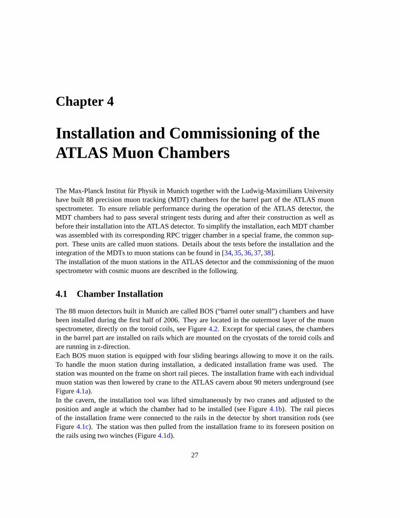
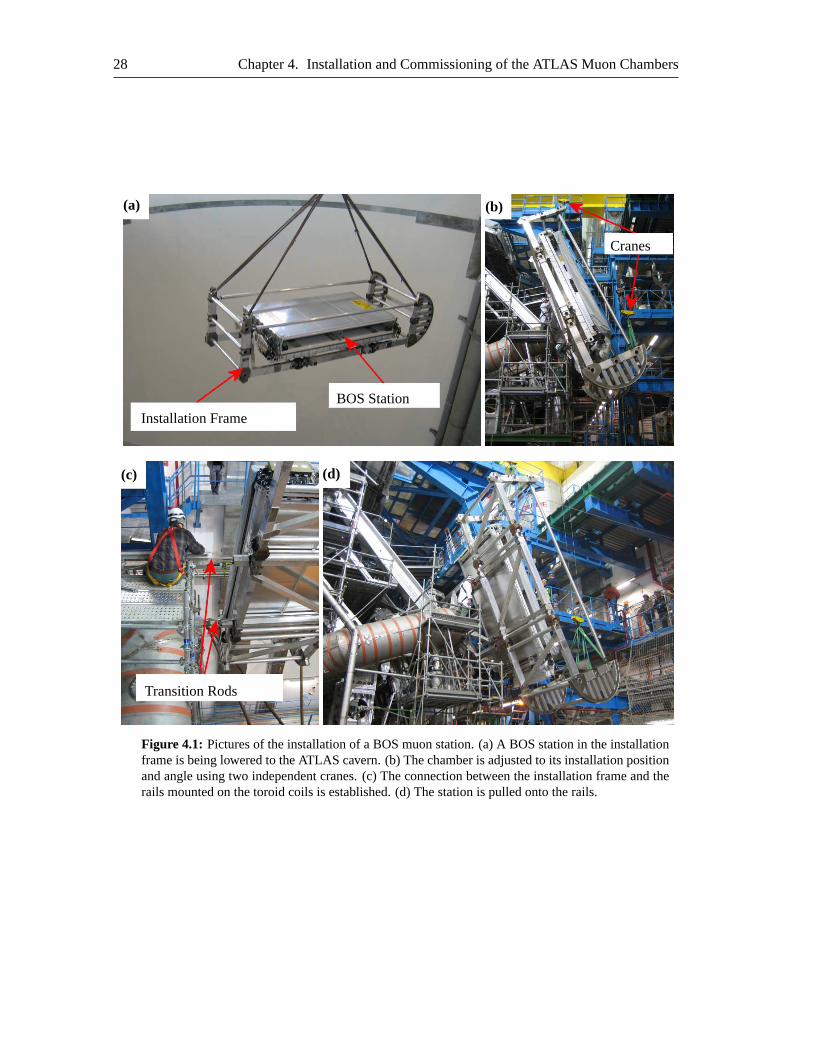
The 88 muon detectors built in Munich are called BOS (“barrel outer small”) chambers and havebeen installed during the first half of 2006. They are located in the outermost layer of the muonspectrometer, directly on the toroid coils, see Figure4.2. Except for special cases, the chambersin the barrel part are installed on rails which are mounted on the cryostats ofthe toroid coils andare running in z-direction.Each BOS muon station is equipped with four sliding bearings allowing to move it onthe rails.To handle the muon station during installation, a dedicated installation frame was used. Thestation was mounted on the frame on short rail pieces. The installation frame witheach individualmuon station was then lowered by crane to the ATLAS cavern about 90 metersunderground (seeFigure4.1a).In the cavern, the installation tool was lifted simultaneously by two cranes and adjusted to theposition and angle at which the chamber had to be installed (see Figure4.1b). The rail piecesof the installation frame were connected to the rails in the detector by short transition rods (seeFigure4.1c). The station was then pulled from the installation frame to its foreseen position onthe rails using two winches (Figure4.1d).
27
28 Chapter 4. Installation and Commissioning of the ATLAS Muon Chambers
Installation FrameBOS Station
(a)
Cranes
(b)
Transition Rods
(c) (d)
Figure 4.1: Pictures of the installation of a BOS muon station. (a) A BOS station in the installationframe is being lowered to the ATLAS cavern. (b) The chamber isadjusted to its installation positionand angle using two independent cranes. (c) The connection between the installation frame and therails mounted on the toroid coils is established. (d) The station is pulled onto the rails.
4.1.C
hamber
Installation29
BOSStations
Figure 4.2: Front view of the barrel part of the ATLAS muon spectrometer after the installation of the muon chambers on the eight toroidcoils. The BOS MDT chambers built in Munich are mounted in theouter layer of the muon spectrometer, directly on the toroidcoils.
30 Chapter 4. Installation and Commissioning of the ATLAS Muon Chambers
-4-4
-2-2
0
0
0
0
2
2
2
2
4
4
4
4
66 88 1010 1212
z−
z nom
inal
[mm
]
MDT ChamberB
OS
6A16
BO
S5A
16B
OS
4A16
BO
S3A
16B
OS
2A16
BO
S1A
16
BO
S6C
16
BO
S5C
16
BO
S4C
16
BO
S3C
16
BO
S2C
16
BO
S1C
16
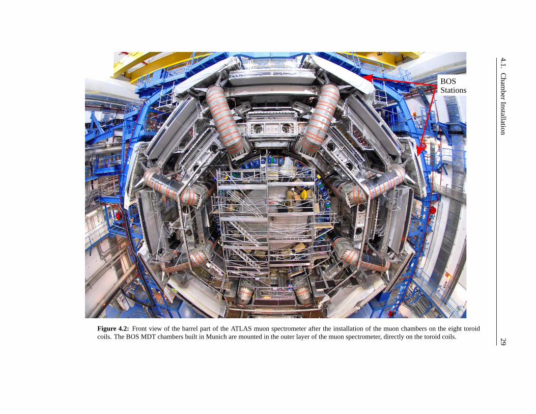
Figure 4.3: Deviation of the BOS MDT chamber positions from the nominal positions after thefinal positioning on the rails in sector 16 of the ATLAS barrelmuon spectrometer. The shaded bandindicates one third of the allowed tolerance of 4 mm.
The exact positioning of the muon stations on the rails and the adjustment of the MDT chamberposition on the common support was performed by hand with an accuracy ofone millimeter.Figure4.3 shows the deviations of the BOS chamber positions from the nominal positions intheglobal ATLAS coordinate system in one typical barrel sector after the final positioning on the rails.All chambers are located well within the allowed range of±4 mm. Special stoppers mounted onthe rails are used to fix the chamber positions on the rails. Adjustment screws on the stoppersallow for a fine tuning of the chamber position along the rails. At the final position, each chamberis only fixed at one of the four bearings in order to prevent stress on thecommon support.
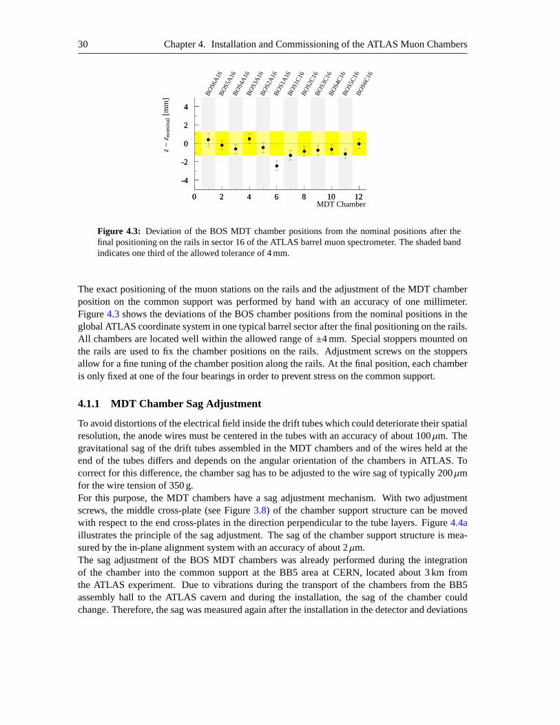
4.1.1 MDT Chamber Sag Adjustment
To avoid distortions of the electrical field inside the drift tubes which could deteriorate their spatialresolution, the anode wires must be centered in the tubes with an accuracy of about 100µm. Thegravitational sag of the drift tubes assembled in the MDT chambers and of thewires held at theend of the tubes differs and depends on the angular orientation of the chambers in ATLAS. Tocorrect for this difference, the chamber sag has to be adjusted to the wire sag of typically 200µmfor the wire tension of 350 g.For this purpose, the MDT chambers have a sag adjustment mechanism. With twoadjustmentscrews, the middle cross-plate (see Figure3.8) of the chamber support structure can be movedwith respect to the end cross-plates in the direction perpendicular to the tubelayers. Figure4.4aillustrates the principle of the sag adjustment. The sag of the chamber supportstructure is mea-sured by the in-plane alignment system with an accuracy of about 2µm.The sag adjustment of the BOS MDT chambers was already performed during the integrationof the chamber into the common support at the BB5 area at CERN, located about 3 km fromthe ATLAS experiment. Due to vibrations during the transport of the chambers from the BB5assembly hall to the ATLAS cavern and during the installation, the sag of the chamber couldchange. Therefore, the sag was measured again after the installation in thedetector and deviations
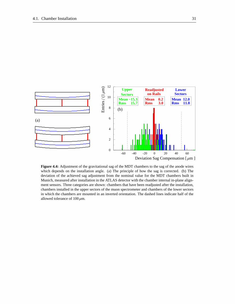
4.1. Chamber Installation 31
0.40
(a)
RmsMean
15.7−15.3
SectorsUpper
RmsMean
11.812.0
SectorsLower
RmsMean
3.0 0.2
on RailsReadjusted
-60 -40 -20 00
2
4
6
8
10
12
20 40 60
Deviation Sag Compensation [µm ]
Ent
ries/
(1µm
)
(b)
Figure 4.4: Adjustment of the gravitational sag of the MDT chambers to the sag of the anode wireswhich depends on the installation angle. (a) The principle of how the sag is corrected. (b) Thedeviation of the achieved sag adjustment from the nominal value for the MDT chambers built inMunich, measured after installation in the ATLAS detector with the chamber internal in-plane align-ment sensors. Three categories are shown: chambers that have been readjusted after the installation,chambers installed in the upper sectors of the muon spectrometer and chambers of the lower sectorsin which the chambers are mounted in an inverted orientation. The dashed lines indicate half of theallowed tolerance of 100µm.

32 Chapter 4. Installation and Commissioning of the ATLAS Muon Chambers
from the nominal sag have been corrected for the accessible chambers.Figure4.4bshows the results of the sag adjustment of the installed BOS muon chambers. Allad-justments are well within the allowed tolerance of±100µm. It can also be seen that the deviationsof the chamber sags in the upper and lower sectors are of opposite sign. An explanation for thiseffect is settling of the sag adjustment screws due to vibrations during the transport of the cham-bers. In contrast to the upper sector chambers, the chambers for the lower sectors were transportedin their installation orientation upside down explaining the opposite sign of the sagdeviations.
4.1.2 Tests After Chamber Installation
The following performance tests of the MDT chambers have been performed immediately aftertheir installation in order to detect damages which could have occurred during the installation:
• Measurement of the gas leak rate of each multilayer to detect damages to the gas system.All 88 BOS MDT chambers fulfill the leak rate requirement within the measurement errors.The largest measured leak rates are only a factor 1.5 above the limit.
• Measurement of the high voltage stability in order to detect broken wires causing short-circuits between the wires and the tube walls or other faults in the high voltage distributionto the drift tubes. No problems have been found concerning the stability of the voltage andthe currents drawn by the chambers.
After the electrical and gas connections were established, a series of further tests of the MDTchambers has been performed:
• Test of the chamber-internal and the chamber-to-chamber alignment systems. No faults havebeen detected.
• Test of the temperature and magnetic field sensors which are mounted on the MDT cham-bers. All magnetic field sensors and≥99.5 % of the temperature sensors are operational.
• Test of the complete chamber read-out chain including the programming of theon-chamberelectronics. Less than 1 percent of the electronics showed errors andhas been replaced.
• Test of the noise rate of all drift tubes with and without high voltage applied.Several BOSchambers showed a significantly higher noise level as before installation. Further investiga-tion revealed that the noise is due to pick-up on the high voltage cables. Additional low-passfilters have been installed and the chambers are now well below the noise limits [39].
4.2 Commissioning of the Muon Spectrometer with Cosmic Muons
The performance of individual muon detectors as well as of the muon spectrometer as a whole canbe studied by means of cosmic ray muons impinging on the ATLAS detector. The measurementsof cosmic muons started right after the installation of the muon stations and were extended suc-cessively. Since the final gas distribution system was not yet operational and the number of power

4.2. Commissioning of the Muon Spectrometer with Cosmic Muons 33
supplies was very limited, the number of muon detectors ready for data-takinginitially was verysmall.At the end of 2005, the first six muon chambers were ready for operation. In November 2006,13 muon chambers were operated when the barrel toroid was ramped up to nominal field for thefirst time, allowing for the measurement of muon momenta. Finally in 2008, the wholemuon spec-trometer (like the other detector components) was ready to take data and more than 200 millioncosmic muons were recorded. In the following, the most important results obtained from thesedata are presented.
4.2.1 Drift Tube Efficiency Measurement
Cosmic muons can be used to determine the detection efficiency of individual drift tubes in MDTchambers by the following algorithm:
• Muon tracks are reconstructed within a MDT chamber using all drift tubes except for thetube under investigation.
• The muon tracks are extrapolated to the tube under investigation.
• The detection efficiencyε of the tube under investigation is given by:
ε =Number of hits detected by the tube
Number of reconstructed tracks traversing the tube
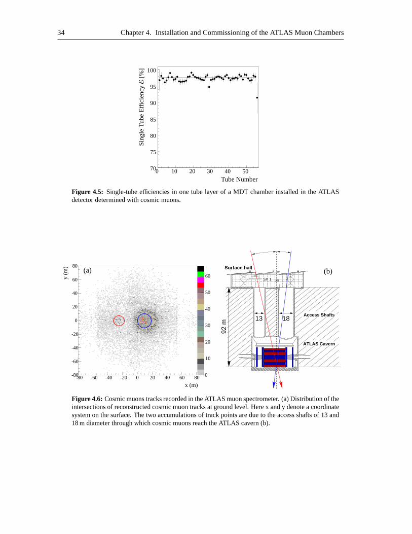
Figure4.5 shows a typical result for one tube layer of a MDT chamber. The drift tubes show anaverage detection efficiency of 97.7±0.1 %, which is consistent with the expected efficiency lossdue to the 400µm thick aluminum walls of the 15 mm diameter drift tubes.Only 1 ‰ of the 338 640 drift tubes of the muon spectrometer had to be permanently disconnectedfrom high voltage and read out due to broken wires or gas leaks.
4.2.2 Reconstruction of Cosmic Muon Tracks
The ATLAS cavern is situated about 90 meters below ground level. Thus, cosmic muons withenergies below∼30 GeV at ground level cannot reach the ATLAS cavern but are absorbed in therock and soil above. However, muons flying through one of the two access shafts with diametersof 13 m and 18 m reach the detector almost unrestrained. Thus, most cosmicmuons recorded inATLAS are constrained into the direction of the access shafts (see Figure4.6b).This was confirmed at the end of 2006 when 13 muon stations were operational allowing for thefirst reconstruction of cosmic muon tracks in the ATLAS muon spectrometer. Figure4.6ashowsthe extrapolation of reconstructed cosmic muon tracks back to the surface.A clear accumulationof tracks on the right part of the plot, as well as a small cluster on the left part are visible. Theseaccumulations agree very well with the positions of the two access shafts.
34 Chapter 4. Installation and Commissioning of the ATLAS Muon Chambers
0 10 20 30 40 5070
75
80
85
90
95
100
Tube Number
Sin
gle
Tub
eEffi
cien
cyE
[%]
Figure 4.5: Single-tube efficiencies in one tube layer of a MDT chamber installed in the ATLASdetector determined with cosmic muons.
-80-80
-60
-60
-40
-40
-20
-20 0
0
0
10
20
20
20
30
40
40
40
50
6060
60
80
80
0.14
y(m
)
x (m)
(a)
13
92 m
18
280 t
20 tSX 1
ATLAS Cavern
Access Shafts
Surface hall(b)
Figure 4.6: Cosmic muons tracks recorded in the ATLAS muon spectrometer. (a) Distribution of theintersections of reconstructed cosmic muon tracks at ground level. Here x and y denote a coordinatesystem on the surface. The two accumulations of track pointsare due to the access shafts of 13 and18 m diameter through which cosmic muons reach the ATLAS cavern (b).
4.2. Commissioning of the Muon Spectrometer with Cosmic Muons 35
Sagitta
Middle layer
Outer layer
Inner layer
y
z
µ
∼5 m
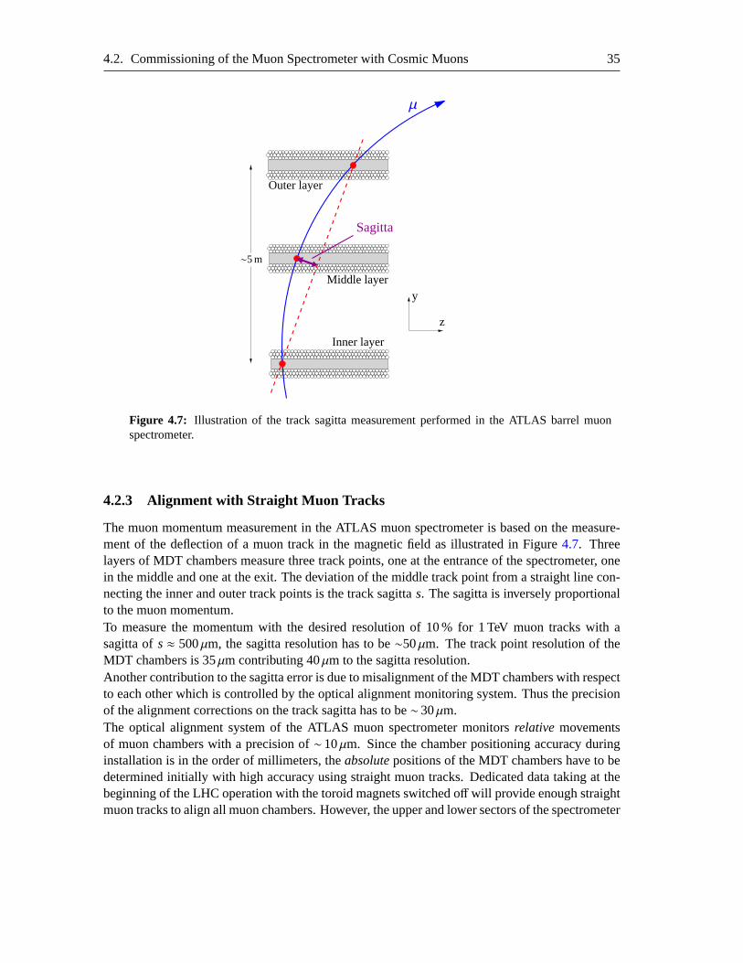
Figure 4.7: Illustration of the track sagitta measurement performed inthe ATLAS barrel muonspectrometer.
4.2.3 Alignment with Straight Muon Tracks
The muon momentum measurement in the ATLAS muon spectrometer is based on the measure-ment of the deflection of a muon track in the magnetic field as illustrated in Figure4.7. Threelayers of MDT chambers measure three track points, one at the entrance of the spectrometer, onein the middle and one at the exit. The deviation of the middle track point from a straight line con-necting the inner and outer track points is the track sagittas. The sagitta is inversely proportionalto the muon momentum.To measure the momentum with the desired resolution of 10 % for 1 TeV muon tracks with asagitta ofs≈ 500µm, the sagitta resolution has to be∼50µm. The track point resolution of theMDT chambers is 35µm contributing 40µm to the sagitta resolution.Another contribution to the sagitta error is due to misalignment of the MDT chambers with respectto each other which is controlled by the optical alignment monitoring system. Thusthe precisionof the alignment corrections on the track sagitta has to be∼30µm.The optical alignment system of the ATLAS muon spectrometer monitorsrelative movementsof muon chambers with a precision of∼10µm. Since the chamber positioning accuracy duringinstallation is in the order of millimeters, theabsolutepositions of the MDT chambers have to bedetermined initially with high accuracy using straight muon tracks. Dedicated data taking at thebeginning of the LHC operation with the toroid magnets switched off will provide enough straightmuon tracks to align all muon chambers. However, the upper and lower sectors of the spectrometer
36 Chapter 4. Installation and Commissioning of the ATLAS Muon Chambers
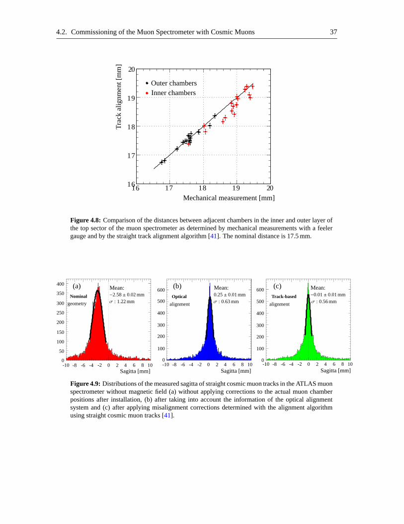
can already be aligned with straight tracks of cosmic muons with switched offmagnetic field. Forthe other sectors horizontal muon tracks are needed, but the rate of horizontal cosmic muons inthe ATLAS cavern is too low.The relative chamber positions within the complete top sector of the barrel muonspectrometer(see Figure3.7) have been determined with a data sample of 400 000 straight cosmic muons usinga linearizedχ2-minimization alignment algorithm [40,41,39]. The distances inzbetween adjacentMDT chambers of the inner and outer layer of the top sector obtained from the track alignmentalgorithm can be compared to measurements of the distances between the tube walls of adjacentchambers using a feeler gauge which have an accuracy of about 50µm (see Figure4.8). A clearcorrelation between the two measurements can be seen. For the outer chambers, the measurementsagree within 85µm while for the inner chamber layer a relative shift of 190µm is observed whichcan be explained by the less accurate method used for the mechanical distance measurement be-tween the inner chambers. The deviations in the order of±1-2 mm from the nominal distance of17.5 mm are consistent with the expectation from the chamber positioning accuracy on the rails(see for example Figure4.3).Another way to verify the alignment procedure is by looking at the sagitta distribution of straighttracks. In the absence of a magnetic field, the muon tracks are straight anda misalignment ofthe MDT chambers will cause a deviation of the sagitta measurement from zero(false sagitta).Figure4.9ashows the distribution of the false sagitta of cosmic muons measured in a chambertriplet in the top sector of the muon spectrometer without magnetic field and assuming nominaldetector geometry in the reconstruction. The distribution peaks at−2.6 mm which is consistentwith the expected deviations of the actual chamber positions from the nominal geometry. If thechamber displacements measured by the optical alignment system (using a preliminary calibration)are taken into account in the sagitta calculation, the peak of the distribution is shifted to+0.25 mm(see Figure4.9b). Using the updated information of the chamber positions from the straight trackalignment algorithm, the measured sagitta distribution peaks at−10µm (see Figure4.9c) which iswell within the required accuracy of±30µm.The width of the distributions is getting smaller if the alignment corrections are applied. This canbe explained by taking into account rotations of the chambers measured by the optical and straighttrack alignment algorithm. The remaining width of about half a millimeter and the tails ofthesagitta distribution of aligned chambers (Figure4.9c) can be explained by deviations from straighttracks due to multiple scattering of the muons.
4.2.4 Curved Muon Tracks
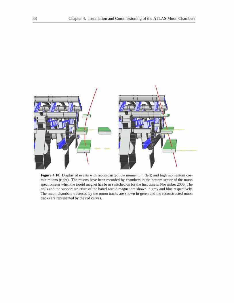
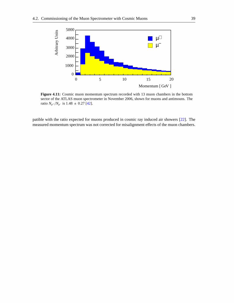
An important milestone in the commissioning of the muon spectrometer was reached when thebarrel toroid magnet was switched on for the first time after assembly in the underground cavern.On 18 November 2006, the barrel toroid was successfully ramped up to thenominal current of20.5 kA. Thus, the 13 muon chambers fully operational at this time could record the first curvedcosmic muon tracks. Two examples are shown in Figure4.10 in the ATLAS event display: onthe left-hand side a low-momentum muon track withpT = 1.6 GeV and on the right-hand side ahigh-momentum muon withpT ∼ 200 GeV.In Figure 4.11 the momentum distributions of the recorded cosmic muons and antimuons areshown. The observed ratio of the two charge componentsNµ+/Nµ− = 1.48 ± 0.27 [42] is com-
4.2. Commissioning of the Muon Spectrometer with Cosmic Muons 37
0
0
1
1
1
1 1111
2
266
7
7
8
8
9
9Mechanical measurement [mm]
Tra
ckal
ignm
ent[
mm
]
Inner chambersOuter chambers
Figure 4.8: Comparison of the distances between adjacent chambers in the inner and outer layer ofthe top sector of the muon spectrometer as determined by mechanical measurements with a feelergauge and by the straight track alignment algorithm [41]. The nominal distance is 17.5 mm.
-10 -10 -10-8 -8 -8-6 -6 -6-4 -4 -4-2 -2 -20 00 0 0
02 2 24 4 46 6 68 8 810 10 10
50
100100 100
150
200
200 200
250
300
300 300
350
400
400 400
500 500
600 600
0.40
Sagitta [mm]Sagitta [mm] Sagitta [mm]
Mean: Mean:Mean:−2.58± 0.02 mm 0.25± 0.01 mm −0.01± 0.01 mmσ : 1.22 mm σ : 0.63 mm σ : 0.56 mm
Nominal
geometry
Optical
alignment alignment
Track-based
(a) (b) (c)
Figure 4.9: Distributions of the measured sagitta of straight cosmic muon tracks in the ATLAS muonspectrometer without magnetic field (a) without applying corrections to the actual muon chamberpositions after installation, (b) after taking into account the information of the optical alignmentsystem and (c) after applying misalignment corrections determined with the alignment algorithmusing straight cosmic muon tracks [41].
38 Chapter 4. Installation and Commissioning of the ATLAS Muon Chambers
0.26
Figure 4.10: Display of events with reconstructed low momentum (left) and high momentum cos-mic muons (right). The muons have been recorded by chambers in the bottom sector of the muonspectrometer when the toroid magnet has been switched on forthe first time in November 2006. Thecoils and the support structure of the barrel toroid magnet are shown in gray and blue respectively.The muon chambers traversed by the muon tracks are shown in green and the reconstructed muontracks are represented by the red curves.
4.2. Commissioning of the Muon Spectrometer with Cosmic Muons 39
µµ − +
00 5 10 15 20
1000
2000
3000
4000
5000
Arb
itrar
yU
nits
Momentum [ GeV ]
Figure 4.11: Cosmic muon momentum spectrum recorded with 13 muon chambers in the bottomsector of the ATLAS muon spectrometer in November 2006, shown for muons and antimouns. Theratio Nµ+/Nµ− is 1.48 ± 0.27 [42].
patible with the ratio expected for muons produced in cosmic ray induced air showers [22]. Themeasured momentum spectrum was not corrected for misalignment effects of the muon chambers.

Chapter 5
The Search for the Higgs Boson
This chapter introduces the ingredients needed for the search for the Higgs boson produced byvector-boson fusion and subsequently decaying into twoτ leptons. In this work the fully leptonicas well as the semileptonic final state of the further decayingτ-lepton pair is taken into account.Characteristic features of the studied search channel and the associated background processes aswell as the used data samples are described in Section5.1. The expected reconstruction and identi-fication performance of the objects relevant for the Higgs boson searchis discussed in Section5.2.Although neutrinos from theτ-lepton decays are present in the final state, it is still possible to re-construct the Higgs boson mass by the collinear approximation which is described in Section5.3.Section5.4finally gives a detailed description of various discriminating variables that can be usedin order to distinguish signal and background events.
In the subsequent chapters, two approaches for separating signal and background processes areshown – an analysis based on successive cuts on several discriminatingvariables (Chapter6) andan approach based on multivariate techniques that takes into account correlations between differentdiscriminating variables (Chapter7).The prospects of discovering the Higgs boson after three years of ATLAS operation are discussedin Chapter8 which mainly focusses on the influence of systematic uncertainties from theory andthe detector performance on the expected signal significance.Several previous studies have investigated the Higgs boson discovery potential in the vector-bosonfusion H → ττ channel with a cut-based analysis [43,44,45,46,47,48]. The discovery potentialof the ATLAS experiment has recently been studied in the context of the “computing systemcommissioning” (CSC) effort, a test of the worldwide data processing infrastructure which wasalso used to perform large scale simulations and physics analyses [49]. A cut-based analysis inanalogy to this study repeatedly serves as a reference for comparison and is referred to asbaselineanalysisthroughout this work.
5.1 Signal and Background Processes
The Higgs bosons produced through vector-boson fusion (see Section 2.2.2) are accompanied bytwo characteristic jets in the forward region of the detector, the so-called tagging jets. These
41
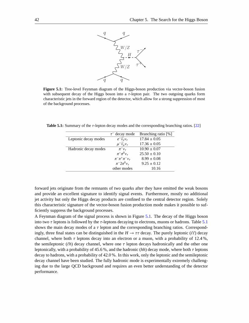
42 Chapter 5. The Search for the Higgs Boson
τ−
τ+
H
q q
q q
W/Z
W/Z
Figure 5.1: Tree-level Feynman diagram of the Higgs-boson production via vector-boson fusionwith subsequent decay of the Higgs boson into aτ-lepton pair. The two outgoing quarks formcharacteristic jets in the forward region of the detector, which allow for a strong suppression of mostof the background processes.
Table 5.1: Summary of theτ-lepton decay modes and the corresponding branching ratios. [22]
τ− decay mode Branching ratio [%]Leptonic decay modes e−νeντ 17.84± 0.05
µ−νµντ 17.36± 0.05Hadronic decay modes π−ντ 10.90± 0.07
π−π0ντ 25.50± 0.10π−π+π−ντ 8.99± 0.08π−2π0ντ 9.25± 0.12
other modes 10.16
forward jets originate from the remnants of two quarks after they have emittedthe weak bosonsand provide an excellent signature to identify signal events. Furthermore, mostly no additionaljet activity but only the Higgs decay products are confined to the central detector region. Solelythis characteristic signature of the vector-boson fusion production mode makes it possible to suf-ficiently suppress the background processes.A Feynman diagram of the signal process is shown in Figure5.1. The decay of the Higgs bosoninto twoτ leptons is followed by theτ-leptons decaying to electrons, muons or hadrons. Table5.1shows the main decay modes of aτ lepton and the corresponding branching ratios. Correspond-ingly, three final states can be distinguished in theH → ττ decay. The purely leptonic (ℓℓ) decaychannel, where bothτ leptons decay into an electron or a muon, with a probability of 12.4 %,the semileptonic (ℓh) decay channel, where oneτ lepton decays hadronically and the other oneleptonically, with a probability of 45.6 %, and the hadronic (hh) decay mode, where bothτ leptonsdecay to hadrons, with a probability of 42.0 %. In this work, only the leptonic and the semileptonicdecay channel have been studied. The fully hadronic mode is experimentally extremely challeng-ing due to the large QCD background and requires an even better understanding of the detectorperformance.
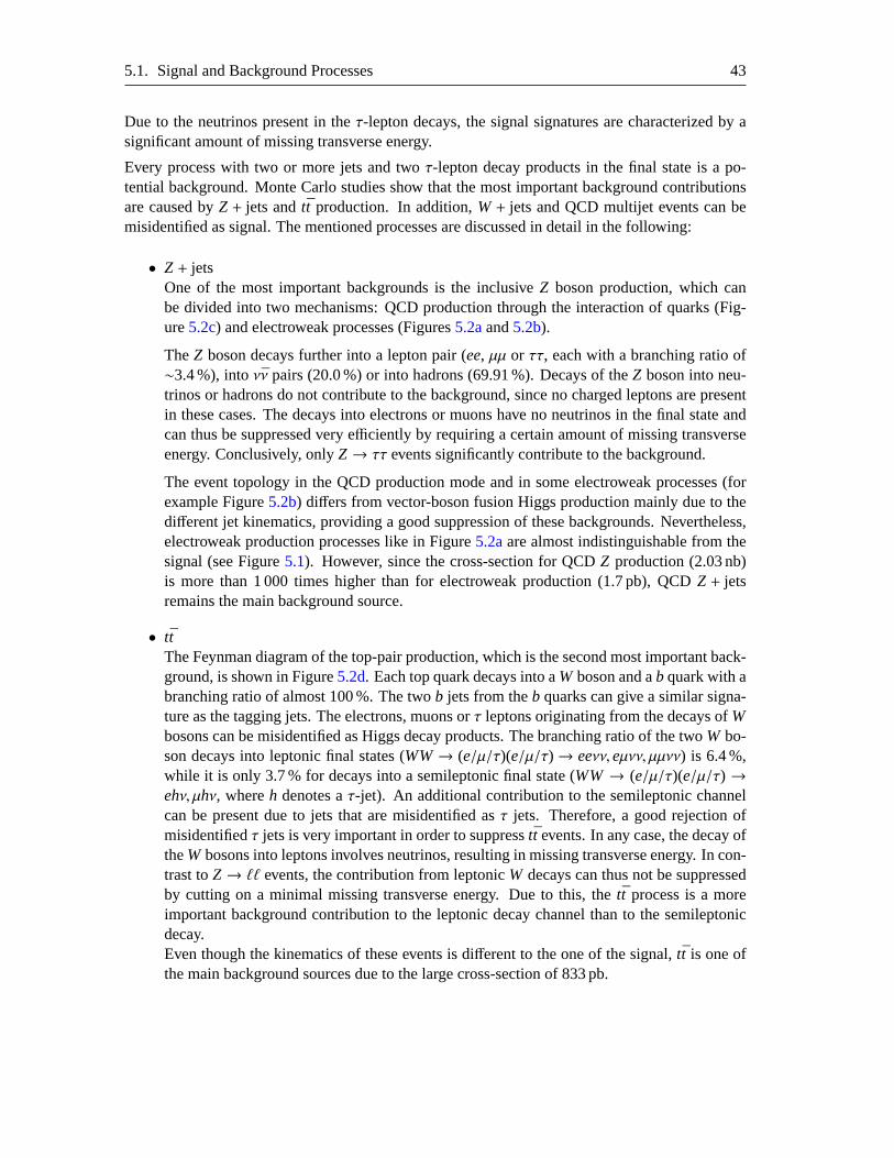
5.1. Signal and Background Processes 43
Due to the neutrinos present in theτ-lepton decays, the signal signatures are characterized by asignificant amount of missing transverse energy.
Every process with two or more jets and twoτ-lepton decay products in the final state is a po-tential background. Monte Carlo studies show that the most important background contributionsare caused byZ + jets andtt production. In addition,W+ jets and QCD multijet events can bemisidentified as signal. The mentioned processes are discussed in detail in thefollowing:
• Z + jetsOne of the most important backgrounds is the inclusiveZ boson production, which canbe divided into two mechanisms: QCD production through the interaction of quarks (Fig-ure5.2c) and electroweak processes (Figures5.2aand5.2b).
TheZ boson decays further into a lepton pair (ee, µµ or ττ, each with a branching ratio of∼3.4 %), intoνν pairs (20.0 %) or into hadrons (69.91 %). Decays of theZ boson into neu-trinos or hadrons do not contribute to the background, since no charged leptons are presentin these cases. The decays into electrons or muons have no neutrinos in thefinal state andcan thus be suppressed very efficiently by requiring a certain amount of missing transverseenergy. Conclusively, onlyZ→ ττ events significantly contribute to the background.
The event topology in the QCD production mode and in some electroweak processes (forexample Figure5.2b) differs from vector-boson fusion Higgs production mainly due to thedifferent jet kinematics, providing a good suppression of these backgrounds. Nevertheless,electroweak production processes like in Figure5.2aare almost indistinguishable from thesignal (see Figure5.1). However, since the cross-section for QCDZ production (2.03 nb)is more than 1 000 times higher than for electroweak production (1.7 pb), QCDZ + jetsremains the main background source.
• ttThe Feynman diagram of the top-pair production, which is the second most important back-ground, is shown in Figure5.2d. Each top quark decays into aW boson and ab quark with abranching ratio of almost 100 %. The twob jets from theb quarks can give a similar signa-ture as the tagging jets. The electrons, muons orτ leptons originating from the decays ofWbosons can be misidentified as Higgs decay products. The branching ratioof the twoW bo-son decays into leptonic final states (WW→ (e/µ/τ)(e/µ/τ)→ eeνν,eµνν, µµνν) is 6.4 %,while it is only 3.7 % for decays into a semileptonic final state (WW→ (e/µ/τ)(e/µ/τ) →ehν, µhν, whereh denotes aτ-jet). An additional contribution to the semileptonic channelcan be present due to jets that are misidentified asτ jets. Therefore, a good rejection ofmisidentifiedτ jets is very important in order to suppresstt events. In any case, the decay oftheW bosons into leptons involves neutrinos, resulting in missing transverse energy. In con-trast toZ→ ℓℓ events, the contribution from leptonicW decays can thus not be suppressedby cutting on a minimal missing transverse energy. Due to this, thett process is a moreimportant background contribution to the leptonic decay channel than to the semileptonicdecay.Even though the kinematics of these events is different to the one of the signal,tt is one ofthe main background sources due to the large cross-section of 833 pb.
44 Chapter 5. The Search for the Higgs Boson
• W+ jetsThe production of a singleW boson with additional jets in the event is another potentialbackground, in particular to the semileptonic decay mode. A signature similar to thesignalis given by theW decays into electrons or muons, with an additional jet in the event fakingtheτ jet. In case two more jets are present in the event, they can be misidentified as taggingjets. Thus, at least three additional jets are needed to contribute to the background. TheW+ jets background can be significantly reduced by a cut on the transversemassmℓνT (seeSection5.4.1) of the lepton and the missing transverse energyEmiss
T . A Feynman diagramof theW+ jets production is shown in Figure5.2e.
• WW+ jetsAs shown in Figure5.2f, the production of aWW pair can also provide a signature whichis quite similar to the signal. However, the cross-section of this process (112pb) is∼20times lower than the one for theZ boson production. Also the kinematic properties differsignificantly from the signal, since the neutrinos are not collinearly emitted with the Wbosons. Correspondingly, theWW+ jets background contribution is much less importantthan theZ + jets production and has been neglected in this study.
• QCDSince the LHC is a proton-proton collider, the cross-section for multijet production is veryhigh. Fortunately, no isolated leptons are present in these events such that the QCD eventsare strongly suppressed by the requirement of twoτ-decay products in the final state.Potential background is caused by events containing misidentified leptons orleptons fromb meson decays. Therefore, an excellent suppression of misidentified electrons, muons andτ jets is crucial for a discovery of the Higgs boson in this channel. The remaining bb back-ground containing real leptons fromb decays can be efficiently suppressed by requiring thatthe leptons are isolated.
5.1.1 Monte Carlo Simulation
Several different Monte Carlo event generators have been used to simulate the signaland back-ground processes. The simulated data samples and the corresponding cross-sections are summa-rized in Tables5.2, 5.3, 5.4 and5.5. All datasets have been produced in the frame of the centralATLAS Monte Carlo production with the Athena software framework (release 12.0.6) [50].
The events generated by the Monte Carlo generators are passed through the detailed simulationof the ATLAS detector based on the G4 [51] package for the description of the detector re-sponse. In case of thett background, the detailed detector simulation has been exchanged by theparameterized and thus faster simulation of the detector response by means of the ATLFAST [52]package. This was the only possibility to obtain a sufficient number of events needed for statisti-cally significant analysis results.
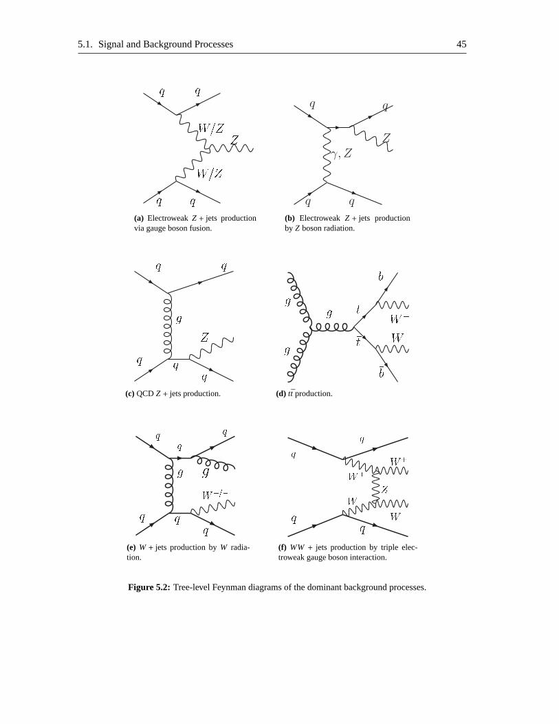
5.1. Signal and Background Processes 45
ZW=ZW=Zqq
(a) ElectroweakZ + jets productionvia gauge boson fusion.
q q
γ, ZZ
(b) ElectroweakZ + jets productionby Z boson radiation.q q
gqq Zq
(c) QCD Z + jets production.
gg g t�t �b
bW�W+
(d) tt production.
gq �q
qW+=�gq q
q(e) W+ jets production byW radia-tion.
q qqq W+ ZW+
W�W�(f) WW + jets production by triple elec-troweak gauge boson interaction.
Figure 5.2: Tree-level Feynman diagrams of the dominant background processes.
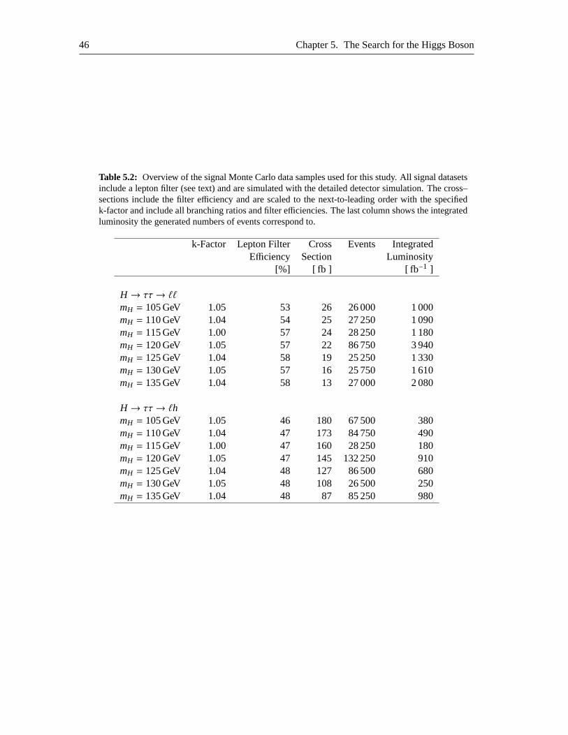
46 Chapter 5. The Search for the Higgs Boson
Table 5.2: Overview of the signal Monte Carlo data samples used for thisstudy. All signal datasetsinclude a lepton filter (see text) and are simulated with the detailed detector simulation. The cross–sections include the filter efficiency and are scaled to the next-to-leading order with the specifiedk-factor and include all branching ratios and filter efficiencies. The last column shows the integratedluminosity the generated numbers of events correspond to.
k-Factor Lepton Filter Cross Events IntegratedEfficiency Section Luminosity
[%] [ fb ] [ fb −1 ]
H → ττ→ ℓℓmH = 105 GeV 1.05 53 26 26 000 1 000mH = 110 GeV 1.04 54 25 27 250 1 090mH = 115 GeV 1.00 57 24 28 250 1 180mH = 120 GeV 1.05 57 22 86 750 3 940mH = 125 GeV 1.04 58 19 25 250 1 330mH = 130 GeV 1.05 57 16 25 750 1 610mH = 135 GeV 1.04 58 13 27 000 2 080
H → ττ→ ℓhmH = 105 GeV 1.05 46 180 67 500 380mH = 110 GeV 1.04 47 173 84 750 490mH = 115 GeV 1.00 47 160 28 250 180mH = 120 GeV 1.05 47 145 132 250 910mH = 125 GeV 1.04 48 127 86 500 680mH = 130 GeV 1.05 48 108 26 500 250mH = 135 GeV 1.04 48 87 85 250 980
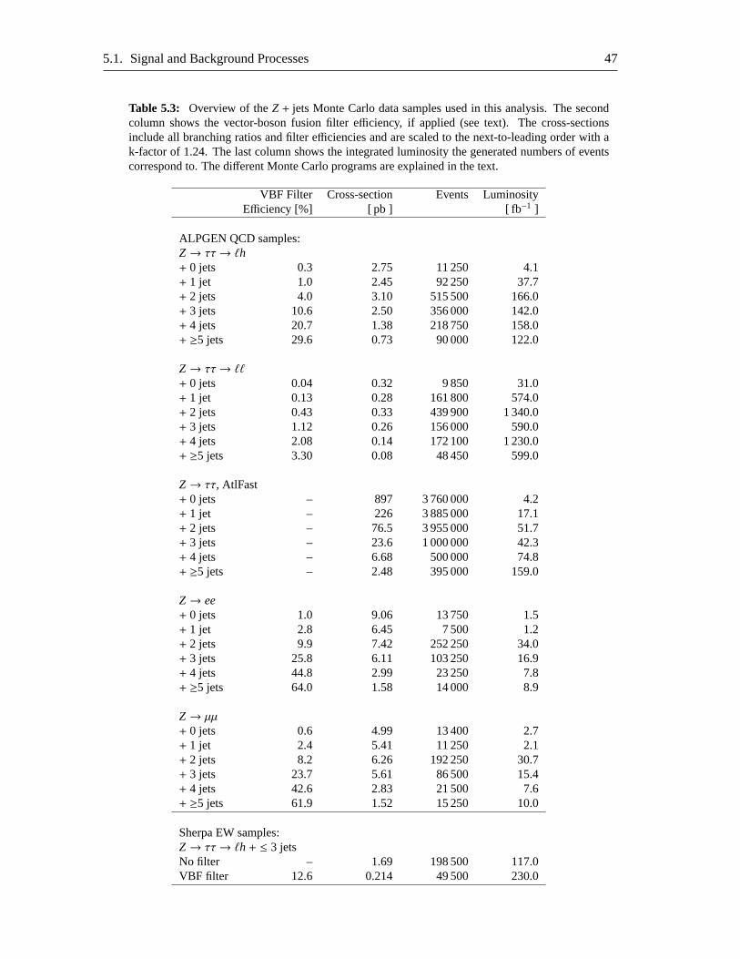
5.1. Signal and Background Processes 47
Table 5.3: Overview of theZ + jets Monte Carlo data samples used in this analysis. The secondcolumn shows the vector-boson fusion filter efficiency, if applied (see text). The cross-sectionsinclude all branching ratios and filter efficiencies and are scaled to the next-to-leading order with ak-factor of 1.24. The last column shows the integrated luminosity the generated numbers of eventscorrespond to. The different Monte Carlo programs are explained in the text.
VBF Filter Cross-section Events LuminosityEfficiency [%] [ pb ] [ fb−1 ]
ALPGEN QCD samples:Z→ ττ→ ℓh+ 0 jets 0.3 2.75 11 250 4.1+ 1 jet 1.0 2.45 92 250 37.7+ 2 jets 4.0 3.10 515 500 166.0+ 3 jets 10.6 2.50 356 000 142.0+ 4 jets 20.7 1.38 218 750 158.0+ ≥5 jets 29.6 0.73 90 000 122.0
Z→ ττ→ ℓℓ+ 0 jets 0.04 0.32 9 850 31.0+ 1 jet 0.13 0.28 161 800 574.0+ 2 jets 0.43 0.33 439 900 1 340.0+ 3 jets 1.12 0.26 156 000 590.0+ 4 jets 2.08 0.14 172 100 1 230.0+ ≥5 jets 3.30 0.08 48 450 599.0
Z→ ττ, AtlFast+ 0 jets – 897 3 760 000 4.2+ 1 jet – 226 3 885 000 17.1+ 2 jets – 76.5 3 955 000 51.7+ 3 jets – 23.6 1 000 000 42.3+ 4 jets – 6.68 500 000 74.8+ ≥5 jets – 2.48 395 000 159.0
Z→ ee+ 0 jets 1.0 9.06 13 750 1.5+ 1 jet 2.8 6.45 7 500 1.2+ 2 jets 9.9 7.42 252 250 34.0+ 3 jets 25.8 6.11 103 250 16.9+ 4 jets 44.8 2.99 23 250 7.8+ ≥5 jets 64.0 1.58 14 000 8.9
Z→ µµ+ 0 jets 0.6 4.99 13 400 2.7+ 1 jet 2.4 5.41 11 250 2.1+ 2 jets 8.2 6.26 192 250 30.7+ 3 jets 23.7 5.61 86 500 15.4+ 4 jets 42.6 2.83 21 500 7.6+ ≥5 jets 61.9 1.52 15 250 10.0
Sherpa EW samples:Z→ ττ→ ℓh + ≤ 3 jetsNo filter – 1.69 198 500 117.0VBF filter 12.6 0.214 49 500 230.0
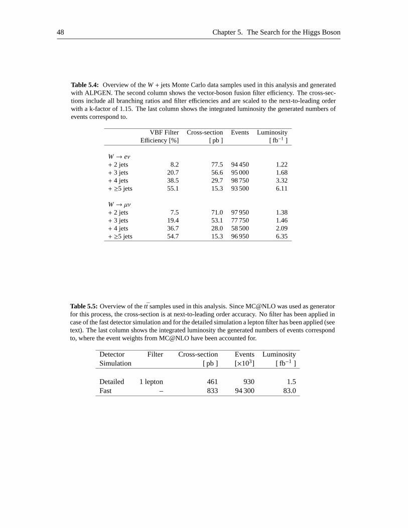
48 Chapter 5. The Search for the Higgs Boson
Table 5.4: Overview of theW+ jets Monte Carlo data samples used in this analysis and generatedwith ALPGEN. The second column shows the vector-boson fusion filter efficiency. The cross-sec-tions include all branching ratios and filter efficiencies and are scaled to the next-to-leading orderwith a k-factor of 1.15. The last column shows the integratedluminosity the generated numbers ofevents correspond to.
VBF Filter Cross-section Events LuminosityEfficiency [%] [ pb ] [ fb−1 ]
W→ eν+ 2 jets 8.2 77.5 94 450 1.22+ 3 jets 20.7 56.6 95 000 1.68+ 4 jets 38.5 29.7 98 750 3.32+ ≥5 jets 55.1 15.3 93 500 6.11
W→ µν+ 2 jets 7.5 71.0 97 950 1.38+ 3 jets 19.4 53.1 77 750 1.46+ 4 jets 36.7 28.0 58 500 2.09+ ≥5 jets 54.7 15.3 96 950 6.35
Table 5.5: Overview of thett samples used in this analysis. Since MC@NLO was used as generatorfor this process, the cross-section is at next-to-leading order accuracy. No filter has been applied incase of the fast detector simulation and for the detailed simulation a lepton filter has been applied (seetext). The last column shows the integrated luminosity the generated numbers of events correspondto, where the event weights from MC@NLO have been accounted for.
Detector Filter Cross-section Events LuminositySimulation [ pb ] [×103] [ fb−1 ]
Detailed 1 lepton 461 930 1.5Fast – 833 94 300 83.0
5.1. Signal and Background Processes 49
Monte Carlo Generators
The Monte Carlo generators used for this study are briefly described in the following:
• Pythia [53]A general-purpose generator for hadronic interactions in leading order with parton show-ering for initial and final state QCD radiation, which leads to relatively soft jets. No spincorrelations are taken into account.
• Herwig [54]Another leading order general-purpose generator with a slightly different parton showeringcompared to Pythia. Herwig is particularly sophisticated in treating the decays of unsta-ble particles with full spin correlation. The Jimmy program [55] is used to simulate theunderlying event. Most of the signal samples have been simulated with Herwig.
• ALPGEN [56]A leading order generator with a different method to match the jets from the parton-showeringmodel to the ones from matrix-element calculations, leading to harder jets. Special emphasisis given to final states with large jet multiplicities, based on exact leading orderevaluationof partonic matrix elements. It is also interfaced to Herwig/Jimmy for the hadronization andunderlying event simulation. ALPGEN was used to simulate the QCDZ + jets backgroundprocesses.
• Sherpa [57]A relatively new multipurpose generator for hadronic events with the matrix element gen-erator AMEGIC++ [58]. Since Sherpa also includes electroweak processes, it was used tosimulate the electroweakZ→ ττ background.
• MC@NLO [59]The only next-to-leading order generator for QCD processes. Like for ALPGEN, MC@NLOwas also interfaced to Herwig/Jimmy for the hadronization and underlying event simulation.Since higher order effects are particularly important fortt production, MC@NLO was usedto generate this background.
All τ-lepton decays have not been simulated by the generators themselves, butby Tauola [60].
Event Filter To increase the background statistics in the phase space of interest event filters havebeen applied at the generator level to save CPU time by eliminating events that would not survivejet related cuts in the analysis.
Lepton filter for signal samples:
• With the numberNℓ of electrons plus muons withpT ≥ 5 GeV and|η| ≤ 2.7:Nℓ ≥ 2 for the samplesH → ττ→ ℓhNℓ ≥ 1 for theH → ττ→ ℓh samples
50 Chapter 5. The Search for the Higgs Boson
VBF filter for Z events:
• With the numberNℓ of electrons plus muons withpT ≥ 10 GeV and|η| ≤ 2.7:Nℓ ≥ 2 for the samplesZ→ ee, µµ andZ→ ττ→ ℓℓNℓ ≥ 1 for theZ→ ττ→ ℓh samples
• At least two jets (cone algorithm with size∆R≤ 0.4) within |η| ≤ 5.0 andpT ≥ 20 GeV for the highestpT jet andpT ≥ 15 GeV for the second highestpT jet
• A jet pair with an invariant mass ofmj j ≥ 300 GeV and a pseudorapidity separation of∆η j j ≥ 2
Lepton filter fortt:
• At least one electron, muon orτ lepton within|η| ≤ 5.0 from aW decay
Pile-Up At the LHC design luminosity ofL = 1.0 × 1034 cm−2s−1, approximately 23 proton-proton collisions occur every 25 ns. Most of these collisions are elastic and inelastic scatteringevents (minimum bias) but the remnants of these processes are also recorded together with in-teresting interactions in the same bunch crossing (pile-up). The additional particles from pile-upevents potentially cause difficulties in the reconstruction of the hard parton collision process. Forexample, the energy determined for a jet from the interesting event could behigher due to energydeposits from pile-up particles or the pile-up events could result in additional jets in the event. Ifthe pile-up originates from the same bunch crossing as the main interaction, it iscalled in-timepile-up. In addition, there is also an out-of-time pile-up contribution, which means that the contri-bution is from an earlier bunch crossing. This is the case for several detector components whichhave a response- and read out time which is much longer than 25 ns, as forexample the liquidArgon calorimeters or the drift tube detectors of the muon system. Other pile-up contributions arefrom the cavern background or from showers induced by particles from cosmic rays.All these effects are not included in the simulated data used in this study as there have not beenenough Monte Carlo datasets including pile-up available.
5.1.2 Detector Simulation
The detector response to the generated particles can be simulated by means of the detailed detectorsimulation or the fast detector simulation ATLFAST. In the following a brief overview of these twosimulations is given – further details can be found in [50,52].
Full Simulation
The full simulation of the ATLAS detector response is based on a detailed andrealistic descriptionof particle interactions with the detector material as provided by the G4 simulation package.A detailed description of the detector geometry and material distribution is used for the simulation,as well as for the exact map of the magnetic field, the realistic response of theread out electronics
5.2. Detector Performance 51
and the trigger behavior. The simulation output is then processed by the samereconstructionalgorithms which will be used for the real collision data. The described simulation process resultsin the best possible predictions but is very time consuming. The full simulation ofone eventtypically takes up to 20 minutes on a standard computer. For that reason, onlya limited numberof events can be fully simulated.
ATLFAST
In order to simulate a large number of events needed for some of the background processes (forexample 100 millions oftt events), the much faster detector simulation software ATLFAST hasbeen used. It is based on a parameterized description of the detector performance. The momentumvectors of the generated particles are smeared and the identification efficiency is parameterizedaccording to studies with the full detector simulation performed for the most important physicsprocesses. A homogeneous magnetic field is assumed in the inner detector volume and a verysimplified calorimeter model is used to simulate the calorimeter response. No difference betweenelectromagnetic and hadronic calorimeter and no longitudinal segmentation of the calorimeters istaken into account. The lateral segmentation is approximated as∆η × ∆φ = 0.1× 0.1 for |η| < 3.2and∆η×∆φ = 0.2×0.2 for 3.2 < |η| < 5.0. The energy of a generated shower particle is depositedin only one calorimeter cell. A cone cluster algorithm with a cone size of∆R=
√
∆η2 + ∆φ2 = 0.4is applied to all cells with a deposited energy above 1.5 GeV. The resulting clusters are associatedwith the originally generated electrons, photons, jets orτ jets.The fast simulation of the detector takes only a few seconds per event. Clearly, the results obtainedby the fast simulation depend on the accuracy of the parameterization of the detector responseand are not as realistic as the ones obtained from full simulation. For this analysis, the mostimportant difference between the detailed detector simulation and ATLFAST is the underestimatedprobability for τ-jet misidentification in the fast simulation. The uncertainties originating fromATLFAST for the background estimation are estimated in Section6.6.3and the influence on thediscovery potential is discussed in Section8.2.2.
5.2 Detector Performance
The following section summarizes the expected performance of the ATLAS detector in recon-structing objects used in this analysis (trigger, electrons, muons, jets,τ jets,b jets and the missingtransverse energy) is summarized – further details can be found in [28]. One of the most importantdetector performance measures is the efficiency of reconstructing and identifying the mentionedobjects. The efficiency is defined as the fraction of reconstructed and correctly identifiedobjectsof the total number of generated objects:
Efficiency=Nmatched
Ngenerated(5.1)
whereNgeneratedis the number of generated objects andNmatchedis the number of objects that havebeen reconstructed and correctly identified and can be matched to a generated object within a smallη − φ−cone. The radiusRof the cone depends on the type of object:R= 0.1 for electrons, muonsandτ jets,R= 0.4 for jets.
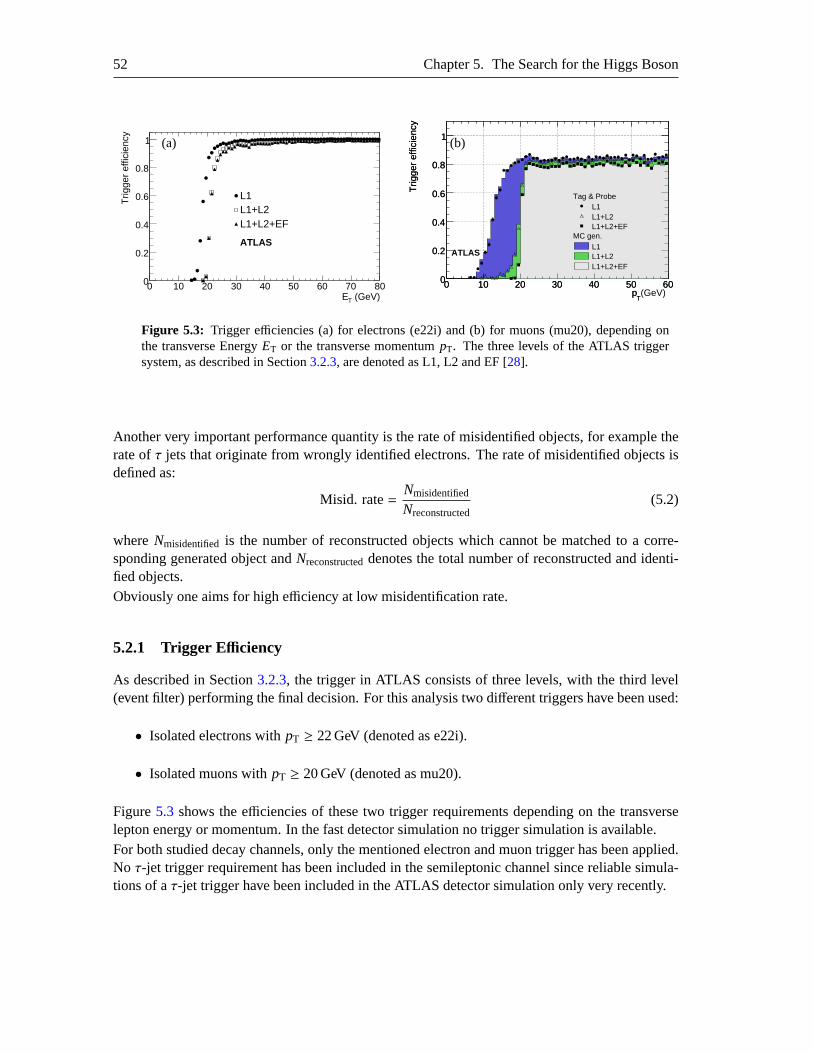
52 Chapter 5. The Search for the Higgs Boson
(GeV)TE0 10 20 30 40 50 60 70 80
Trig
ger
effic
ienc
y
0
0.2
0.4
0.6
0.8
1
L1L1+L2L1+L2+EF
ATLAS
(a)
(GeV)T
p0 10 20 30 40 50 60
Trig
ger
effic
ienc
y
0
0.2
0.4
0.6
0.8
1
Tag & ProbeL1L1+L2L1+L2+EF
MC gen.L1L1+L2L1+L2+EF
Tp
0 10 20 30 40 50 60
Trig
ger
effic
ienc
y
0
0.2
0.4
0.6
0.8
1
ATLAS
(b)
Figure 5.3: Trigger efficiencies (a) for electrons (e22i) and (b) for muons (mu20), depending onthe transverse EnergyET or the transverse momentumpT. The three levels of the ATLAS triggersystem, as described in Section3.2.3, are denoted as L1, L2 and EF [28].
Another very important performance quantity is the rate of misidentified objects, for example therate ofτ jets that originate from wrongly identified electrons. The rate of misidentified objects isdefined as:
Misid. rate=Nmisidentified
Nreconstructed(5.2)
whereNmisidentified is the number of reconstructed objects which cannot be matched to a corre-sponding generated object andNreconstructeddenotes the total number of reconstructed and identi-fied objects.Obviously one aims for high efficiency at low misidentification rate.
5.2.1 Trigger Efficiency
As described in Section3.2.3, the trigger in ATLAS consists of three levels, with the third level(event filter) performing the final decision. For this analysis two different triggers have been used:
• Isolated electrons withpT ≥ 22 GeV (denoted as e22i).
• Isolated muons withpT ≥ 20 GeV (denoted as mu20).
Figure5.3 shows the efficiencies of these two trigger requirements depending on the transverselepton energy or momentum. In the fast detector simulation no trigger simulation is available.For both studied decay channels, only the mentioned electron and muon trigger has been applied.No τ-jet trigger requirement has been included in the semileptonic channel sincereliable simula-tions of aτ-jet trigger have been included in the ATLAS detector simulation only very recently.
5.2. Detector Performance 53
5.2.2 Electron Reconstruction
The reconstruction and identification of electrons [49, 28] in the detailed simulation starts withthe information of the electromagnetic calorimeter. An algorithm searches for spatially groupedcalorimeter cells with a significant energy deposition (cluster). To suppress photons, each clusterhas to be matched to a track of the inner detector. Several additional requirements can be used tofurther suppress the contribution from photons and jets:
• Calorimeter information:Due to the fine granularity of the electromagnetic calorimeter, the lateral and longitudinalshower shape is used to separate electromagnetic from hadronic showers. Also the amountof energy deposited in the hadronic calorimeter, which should be very low inthe case ofelectrons, provides a good suppression of jets.
• Inner detector information:A minimum number of hits in the pixel and SCT detectors, a large energy deposition in thetransition radiation tracker (TRT) and a transverse impact parameter (minimumdistance ofthe extrapolated track to the beam axis) of|d0| < 0.1 cm is used to identify electrons.
• Cluster–track match criteria:The rejection of jets can be significantly improved by ensuring the consistency betweenthe electromagnetic calorimeter and the inner detector information. A good agreement ofthe extrapolation of the inner detector track to the calorimeter and the cluster position aretypical for electrons. The electron energyE measured in the electromagnetic calorimetershould match the momentump measured in the inner detector. Therefore, requiring theratio E/p to be close to unity provides additional separation power.
In this analysis, all electron candidates withpT > 15 GeV that fulfill the cuts related to thecalorimeter information and have a matched track in the inner detector with at least nine pixeland SCT hits are accepted. The ratioE/p and the TRT requirements are not imposed. This setof requirements is known as “medium” strict electron selection and provides asufficient rejectionof misidentified electrons at adequate efficiency. In addition, an isolation cut is applied, whichrequires that the energy deposited within a cone of radiusR= 0.2 around the electron is less than10 % of the electron energy.In case of the ATLFAST detector simulation, a track is accepted as electron if
• a calorimeter cluster is found within∆R= 0.15 and|η| < 2.5 around a generated electron,
• the sum of all cluster energies within∆R= 0.2 is close to the generated electron energy and
• no additional cluster is found around the generated electron within∆R= 0.4.
If an electron fulfills these requirements, its associated energy is the generated energy, smeared bymeans of a resolution function obtained from test beam studies.The graphs in Figure5.4 show the electron efficiency and rate of misidentified electrons as afunction of pT, η andφ for the signal and thett background from the detailed simulation andfor tt also from the ATLFAST simulation. It can be seen that for the detailed simulation, the
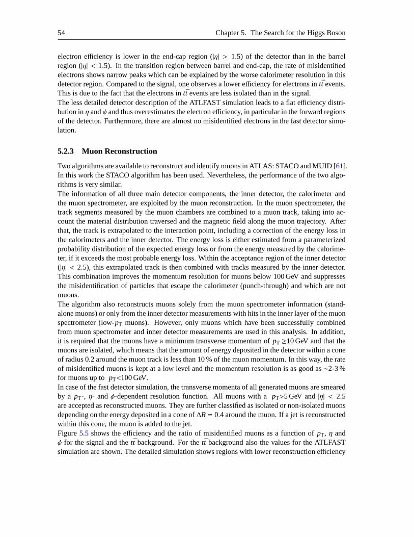
54 Chapter 5. The Search for the Higgs Boson
electron efficiency is lower in the end-cap region (|η| > 1.5) of the detector than in the barrelregion (|η| < 1.5). In the transition region between barrel and end-cap, the rate of misidentifiedelectrons shows narrow peaks which can be explained by the worse calorimeter resolution in thisdetector region. Compared to the signal, one observes a lower efficiency for electrons intt events.This is due to the fact that the electrons intt events are less isolated than in the signal.The less detailed detector description of the ATLFAST simulation leads to a flat efficiency distri-bution inη andφ and thus overestimates the electron efficiency, in particular in the forward regionsof the detector. Furthermore, there are almost no misidentified electrons in thefast detector simu-lation.
5.2.3 Muon Reconstruction
Two algorithms are available to reconstruct and identify muons in ATLAS: STACO and MUID [61].In this work the STACO algorithm has been used. Nevertheless, the performance of the two algo-rithms is very similar.The information of all three main detector components, the inner detector, the calorimeter andthe muon spectrometer, are exploited by the muon reconstruction. In the muon spectrometer, thetrack segments measured by the muon chambers are combined to a muon track, taking into ac-count the material distribution traversed and the magnetic field along the muon trajectory. Afterthat, the track is extrapolated to the interaction point, including a correction of theenergy loss inthe calorimeters and the inner detector. The energy loss is either estimated from a parameterizedprobability distribution of the expected energy loss or from the energy measured by the calorime-ter, if it exceeds the most probable energy loss. Within the acceptance region of the inner detector(|η| < 2.5), this extrapolated track is then combined with tracks measured by the inner detector.This combination improves the momentum resolution for muons below 100 GeV and suppressesthe misidentification of particles that escape the calorimeter (punch-through)and which are notmuons.The algorithm also reconstructs muons solely from the muon spectrometer information (stand-alone muons) or only from the inner detector measurements with hits in the inner layer of the muonspectrometer (low-pT muons). However, only muons which have been successfully combinedfrom muon spectrometer and inner detector measurements are used in this analysis. In addition,it is required that the muons have a minimum transverse momentum ofpT ≥10 GeV and that themuons are isolated, which means that the amount of energy deposited in the detector within a coneof radius 0.2 around the muon track is less than 10 % of the muon momentum. In this way, the rateof misidentified muons is kept at a low level and the momentum resolution is as goodas∼2-3 %for muons up topT<100 GeV.In case of the fast detector simulation, the transverse momenta of all generated muons are smearedby a pT-, η- andφ-dependent resolution function. All muons with apT>5 GeV and|η| < 2.5are accepted as reconstructed muons. They are further classified as isolated or non-isolated muonsdepending on the energy deposited in a cone of∆R= 0.4 around the muon. If a jet is reconstructedwithin this cone, the muon is added to the jet.Figure5.5 shows the efficiency and the ratio of misidentified muons as a function ofpT, η andφ for the signal and thett background. For thett background also the values for the ATLFASTsimulation are shown. The detailed simulation shows regions with lower reconstruction efficiency
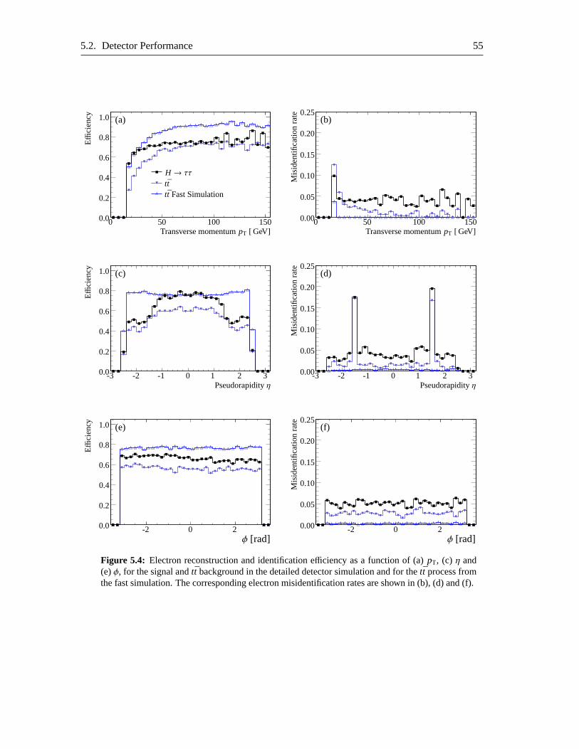
5.2. Detector Performance 55
0 50 100 1500.0
0.2
0.4
0.6
0.8
1.0
QCD
H → ττtttt Fast Simulation
Effi
cien
cy
Transverse momentumpT [ GeV]
(a)
0 50 100 1500.00
0.05
0.10
0.15
0.20
0.25
Mis
iden
tifica
tion
rate
Transverse momentumpT [ GeV]
(b)
-3 -2 -1 0 1 2 30.0
0.2
0.4
0.6
0.8
1.0
Effi
cien
cy
Pseudorapidityη
(c)
-3 -2 -1 0 1 2 30.00
0.05
0.10
0.15
0.20
0.25
Mis
iden
tifica
tion
rate
Pseudorapidityη
(d)
-2 0 20.0
0.2
0.4
0.6
0.8
1.0
0.25
Effi
cien
cy
φ [rad]
(e)
-2 0 20.00
0.05
0.10
0.15
0.20
0.25
Mis
iden
tifica
tion
rate
φ [rad]
(f)
Figure 5.4: Electron reconstruction and identification efficiency as a function of (a)pT, (c) η and(e)φ, for the signal andtt background in the detailed detector simulation and for thett process fromthe fast simulation. The corresponding electron misidentification rates are shown in (b), (d) and (f).
56 Chapter 5. The Search for the Higgs Boson
in theη andφ distribution compared to the fast simulation. Aroundη = 0, the loss of efficiency canbe explained by the gaps in the muon spectrometer due to service connectionsand around|η| = 1.2the lower efficiency is caused by the lower coverage with muon chambers in the barrel–end-captransition region. The small dips atφ = −2.1 andφ = −1.0 are due to the detector feet structurewhich leads to a higher amount of material the muons have to traverse and a lower coverage withmuon chambers.As not all details about the exact detector geometry are incorporated in thefast detector simulation,it shows a flat efficiency distribution inη andφ.
5.2.4 Jet Reconstruction Performance
Jet reconstruction [62] in ATLAS is performed by searching for accumulations of energy depositsin the calorimeter (cluster) which serve as starting points (seeds) for reconstructing jets. Twocluster finding algorithms are available: the “Tower” cluster algorithm which sums up the energydeposits in all calorimeter cells inη − φ bins (two dimensions) and a more sophisticated algorithm,the “Topological” (Topo) cluster algorithm, which reconstructs three-dimensional energy deposi-tions in the calorimeter. The energy clusters found are taken as input to the jet finding algorithms.Again, two jet finding algorithms are available in ATLAS: the so-called “Cone”algorithm and the“kT” algorithm. For this analysis, the Cone algorithm with a cone of∆R= 0.4 and Topo clusterseeds has shown the best performance. This is reflected in the higher efficiency for jets from thevector-boson fusion process in the forward region of the detector.In the fast detector simulation, all clusters with a transverse energy above10 GeV which could notbe assigned to electrons or photons are classified as jets. The jet directionis defined as the clusterdirection and the energies are smeared with the parameterized jet energy resolution.Figure5.6 shows the jet reconstruction efficiency and the ratio of misidentified jets as a functionof pT, η andφ for the signal and thett background. For thett background also the values for theATLFAST simulation are shown. The jet reconstruction efficiency reaches almost 100 % for jetswith a transverse momentum ofpT & 40 GeV and the efficiency shows a rather flat distribution asa function ofη andφ. The jet reconstruction efficiencies in the detailed and in the fast detectorsimulation are very similar to each other.The jet misidentification rate is different for signal andtt background. For the signal the misiden-tification rate of jets is much higher for low transverse momenta within the pseudorapidity rangeof |η| < 2.5. This is due to jets that originate from hadronicτ-lepton decays, which have not beenidentified asτ jets (see Section5.2.5).
5.2.5 τ Jet Reconstruction Performance
For the reconstruction and identification ofτ jets, again two algorithms are available – a track basedapproach showing a higher performance forτ jets with low-pT and the TauRec algorithm [63],which uses calorimeter clusters asτ-jet candidates and has been used in this analysis. Theτ iden-tification in TauRec is based on a likelihood analysis with the following discriminatingvariablesagainst QCD jets:
• The number of tracks associated with the cluster, limited to be either one, two or three.Since in hadronicτ decays there are either one or three charged hadrons, one would ideally
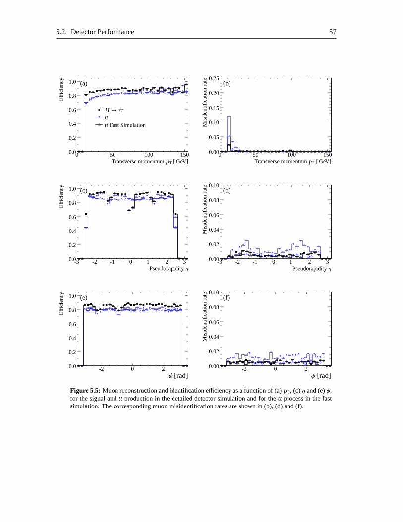
5.2. Detector Performance 57
0 50 100 1500.0
0.2
0.4
0.6
0.8
1.0
QCD
H → ττtttt Fast Simulation
Effi
cien
cy
Transverse momentumpT [ GeV]
(a)
0 50 100 1500.00
0.05
0.10
0.15
0.20
0.25
Mis
iden
tifica
tion
rate
Transverse momentumpT [ GeV]
(b)
-3 -2 -1 0 1 2 30.0
0.2
0.4
0.6
0.8
1.0
Effi
cien
cy
Pseudorapidityη
(c)
-3 -2 -1 0 1 2 30.00
0.02
0.04
0.06
0.08
0.10
Mis
iden
tifica
tion
rate
Pseudorapidityη
(d)
-2 0 20.0
0.2
0.4
0.6
0.8
1.0
0.25
Effi
cien
cy
φ [rad]
(e)
-2 0 20.00
0.02
0.04
0.06
0.08
0.10
Mis
iden
tifica
tion
rate
φ [rad]
(f)
Figure 5.5: Muon reconstruction and identification efficiency as a function of (a)pT, (c)η and (e)φ,for the signal andtt production in the detailed detector simulation and for thett process in the fastsimulation. The corresponding muon misidentification rates are shown in (b), (d) and (f).
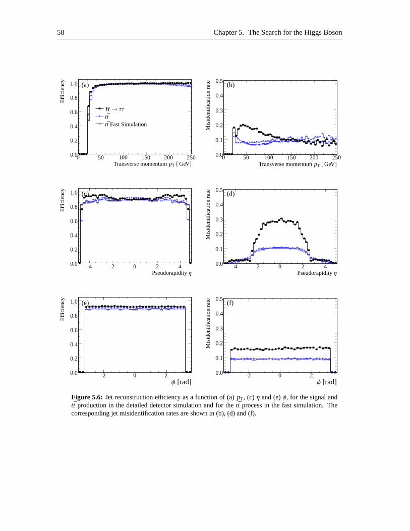
58 Chapter 5. The Search for the Higgs Boson
0 50 100 150 200 2500.0
0.2
0.4
0.6
0.8
1.0
QCD
H → ττtttt Fast Simulation
Effi
cien
cy
Transverse momentumpT [ GeV]
(a)
0 50 100 150 200 2500.0
0.1
0.2
0.3
0.4
0.5
Mis
iden
tifica
tion
rate
Transverse momentumpT [ GeV]
(b)
-4 -2 0 2 40.0
0.2
0.4
0.6
0.8
1.0
Effi
cien
cy
Pseudorapidityη
(c)
-4 -2 0 2 40.0
0.1
0.2
0.3
0.4
0.5
Mis
iden
tifica
tion
rate
Pseudorapidityη
(d)
-2 0 20.0
0.2
0.4
0.6
0.8
1.0
0.25
Effi
cien
cy
φ [rad]
(e)
-2 0 20.0
0.1
0.2
0.3
0.4
0.5
Mis
iden
tifica
tion
rate
φ [rad]
(f)
Figure 5.6: Jet reconstruction efficiency as a function of (a)pT, (c) η and (e)φ, for the signal andtt production in the detailed detector simulation and for thett process in the fast simulation. Thecorresponding jet misidentification rates are shown in (b),(d) and (f).

5.2. Detector Performance 59
expect only one or three tracks. However, one of the three tracks mighthave been missed.(In this analysis,exactlyone or three tracks have been required in addition.)
• The electric charge of theτ jet which is calculated by summing up the charge of all associ-ated tracks should be±1.
• The impact parameter (distance to the primary interaction vertex) of the track with the high-est pT (leading track) associated with theτ candidate. Due to the relatively long life timeof theτ lepton of 2.9 × 10⁻¹³ seconds [22], its decay vertex is displaced from the primaryvertex.
• The radius of the cluster in the electromagnetic calorimeter. Jets from hadronic τ decaystend to be more collimated than QCD jets.
• The fraction of transverse energy in a concentric ring of 0.1< ∆R<0.2 around theτ candi-date cluster should be small, also becauseτ jets are well-collimated.
• The number of hits withET>200 MeV in theη-strip layer of the electromagnetic calorimeter.Hadronically decayingτ leptons typically have a smaller number of hits compared to QCDjets.
• The width of the shower profile in theη-strip layer (see page22) of the electromagneticcalorimeter which tends to be relatively small forτ jets.
• The ratioEhadT /p
1T of the transverse energyEhad
T measured by the hadron calorimeter, and thetransverse momentump1
T of the leading track. In contrast to QCD jets,τ jets tend to have ahigh fraction of their energy associated to the leading track, which leads to arelatively smallEhad
T /p1T ratio.
All τ-jet candidates with a transverse momentum ofpT > 30 GeV and a TauRec log-likelihoodratio of larger than 4.0 are accepted asτ jets. For a further suppression of electrons misidentifiedasτ jets, additional cuts have been applied to theτ-jet candidates:
• A minimum of 0.2 % of the energy of theτ-jet candidate has to be deposited in the first layerof the hadron calorimeter. Electrons usually deposit all their energy in the electromagneticcalorimeter.
• Within the range|η| ≤ 1.7, the ratio of high-threshold (HT) to low-threshold (LT) hits in theTRT has to be smaller than 20 % if there are at least ten LT hits. Due to their higher mass,pions from a hadronicτ decay emit less transition radiation than electrons which results insmaller signals in the TRT.
In case of the fast detector simulation, a jet is considered to be aτ jet if it matches the generatedhadronically decayingτ lepton within a cone of∆R< 0.3 and if the jet energy is comparablewith the visibleτ energy. Subsequently, apT- and η-dependent parameterization of theτ-jetidentification efficiency is applied to eachτ-jet candidate.The performance of theτ-jet reconstruction and identification is shown in Figure5.7. It showsthe efficiency and misidentification rate as a function ofpT, η andφ, for the detailed detector

60 Chapter 5. The Search for the Higgs Boson
simulation of signal andtt background. For thett background also the values for the ATLFASTsimulation are shown.The efficiencies of the three distributions shown are very similar to each other. Theyare rather flatin pT, η andφ and the average efficiency is around 40 % for theτ jets fromtt events and around50 % for theτ jets from the Higgs boson decay. As for the electrons and muons, the slightly lowerτ-jet efficiency in tt events can be explained by theτ jets being less isolated. Compared to thesignal, the rate of misidentifiedτ jets is much higher for thett process in the detailed simulation.This can be explained by the higher jet multiplicity of thett events in the central detector region.With ∼10 %, the rate of misidentifiedτ jets in the fast detector simulation ATLFAST is muchless than in the detailed detector simulation where the rate of misidentifiedτ jets is as high as∼60 %. This difference causes the biggest uncertainty introduced to the analysis of the Higgsboson discovery potential if ATLFAST is used to estimate thett background. In Section6.6.3, theimpact of using ATLFAST data samples in this analysis is discussed.
5.2.6 b Jet Identification
Jets originating fromb quarks show characteristics that can be used to separate them from jetsoriginating from lighter quarks (b-tagging):
• Due to the hard fragmentation (theb hadron has a large fraction of theb quark momentum)and the high masses ofb hadrons (> 5 GeV), the decay products of theb hadron typicallyhave large transverse momenta with respect to the jet axis and thus, their opening angle isalso relatively large.
• The lifetime ofb hadrons of around 1.5 ps is rather long leading to a displacement of theb decay vertex from the primary interaction point of a few millimeters depending on thejet energy. Thus, the impact parameters of the tracks associated with theb hadron decayproducts are rather large.
A likelihood ratio approach [64,28,49] is used to estimate the probability that a jet originated froma b quark. In this analysis, a cut of> 1.0 on the output value of thisb-jet identification algorithm(b-tag weight) is applied to separateb jets from light quark jets.In the fast detector simulation, the identification ofb jets is done in a similar way as for theτ jets. Ajet is labelled asb jet if it can be matched within∆R< 0.2 to a generatedb quark withpT > 5 GeV.In addition, the labelling is stochastically changed for every event using a parameterization of theb-tag efficiency and light quark jet misidentification probability.The expected performance of identifyingb jets with this method is shown in Figure5.8. Thegraphs show theb-jet identification efficiency and the rate of misidentifiedb jets as a function ofpT, η andφ for tt events in the full and the fast detector simulation. It can be seen that the efficiencyas well as the rate of misidentifiedb jets are higher in case of the full detector simulation.
5.2.7 Missing Energy Reconstruction
Since neutrinos do not interact in the detector, they deposit no energy. However, it is possible tocalculate the sum of all neutrino energies in an event in the plane transverse to the beam axis by
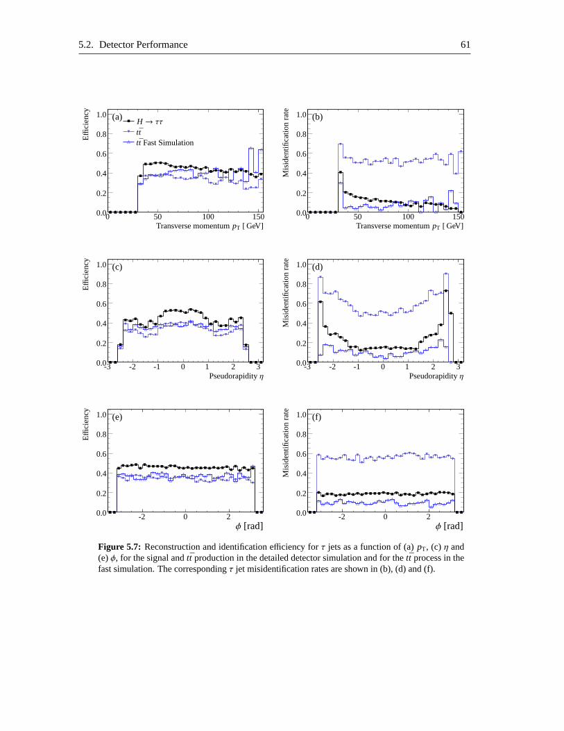
5.2. Detector Performance 61
0 50 100 1500.0
0.2
0.4
0.6
0.8
1.0
QCD
H → ττtttt Fast Simulation
Effi
cien
cy
Transverse momentumpT [ GeV]
(a)
0 50 100 1500.0
0.2
0.4
0.6
0.8
1.0
Mis
iden
tifica
tion
rate
Transverse momentumpT [ GeV]
(b)
-3 -2 -1 0 1 2 30.0
0.2
0.4
0.6
0.8
1.0
Effi
cien
cy
Pseudorapidityη
(c)
-3 -2 -1 0 1 2 30.0
0.2
0.4
0.6
0.8
1.0
Mis
iden
tifica
tion
rate
Pseudorapidityη
(d)
-2 0 20.0
0.2
0.4
0.6
0.8
1.0
0.25
Effi
cien
cy
φ [rad]
(e)
-2 0 20.0
0.2
0.4
0.6
0.8
1.0
Mis
iden
tifica
tion
rate
φ [rad]
(f)
Figure 5.7: Reconstruction and identification efficiency forτ jets as a function of (a)pT, (c) η and(e)φ, for the signal andtt production in the detailed detector simulation and for thett process in thefast simulation. The correspondingτ jet misidentification rates are shown in (b), (d) and (f).
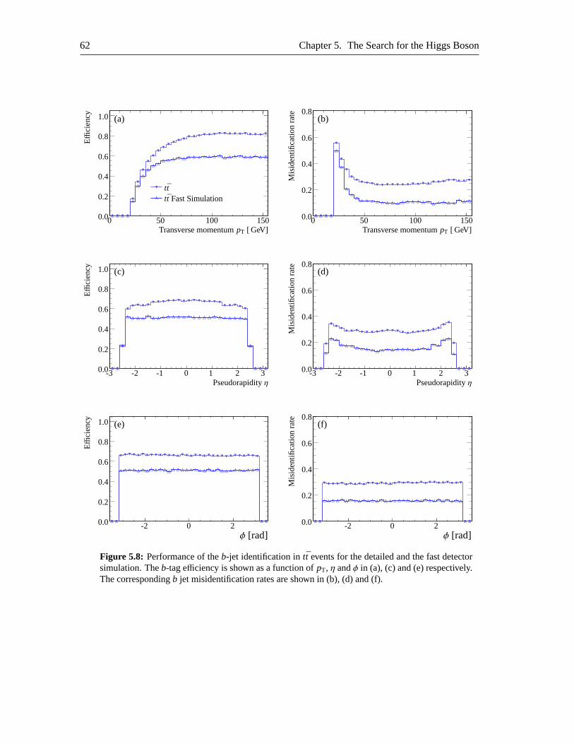
62 Chapter 5. The Search for the Higgs Boson
0 50 100 1500.0
0.2
0.4
0.6
0.8
1.0
QCD
tttt Fast Simulation
Effi
cien
cy
Transverse momentumpT [ GeV]
(a)
0 50 100 1500.0
0.2
0.4
0.6
0.8
Mis
iden
tifica
tion
rate
Transverse momentumpT [ GeV]
(b)
-3 -2 -1 0 1 2 30.0
0.2
0.4
0.6
0.8
1.0
φ
Effi
cien
cy
Pseudorapidityη
(c)
-3 -2 -1 0 1 2 30.0
0.2
0.4
0.6
0.8
Mis
iden
tifica
tion
rate
Pseudorapidityη
(d)
-2 0 20.0
0.2
0.4
0.6
0.8
1.0
0.25
Effi
cien
cy
φ [rad]
(e)
-2 0 20.0
0.2
0.4
0.6
0.8
Mis
iden
tifica
tion
rate
φ [rad]
(f)
Figure 5.8: Performance of theb-jet identification intt events for the detailed and the fast detectorsimulation. Theb-tag efficiency is shown as a function ofpT, η andφ in (a), (c) and (e) respectively.The correspondingb jet misidentification rates are shown in (b), (d) and (f).

5.3. Reconstruction of the Higgs Mass 63
using momentum conservation. The colliding protons do not have transverse momentum compo-nents and therefore the sum of the transverse momenta of all final state particles has to vanish aswell. Thus, the sum of the transverse momenta of all visible final state particlesequals the negativesum of the transverse momenta of all neutrinos.In ATLAS, the calculation of the visible transverse energy is performed in the following way:
• Summation of all calorimeter cell energies, using a calibration independent ofthe incidentparticle type.
• Addition of all muons with an associated high quality track in the inner detector in orderto reduce the influence of misidentified muons. The muon momentum contributing to themissing energy calculation is measured in the muon spectrometer only, providingthe muonenergy after traversing the calorimeters. This ensures that the energy loss of the muons inthe calorimeter is not double-counted.
• Addition of the estimated energy loss in the inactive material, particularly in the liquidArgon calorimeter cryostat walls.
• Refinement of the energy calibration of the contributing calorimeter cells. Since the calorime-ter response depends on the particle type, the energy calibration is also different for differentobjects like, for example, electrons and jets. Thus, the calibration of all calorimeter cellswhich can be associated to a close-by reconstructed object, is replaced by the calibrationspecific for the type of the identified particle.
In the fast detector simulation, all reconstructed objects (photons, electrons, muons,τ jets, QCDjets and unmatched calorimeter clusters) are used to calculate the missing transverse energyEmiss
T .Figure5.9shows the expected resolution of the missing transverse energy measurement from thedetailed detector simulation as a function of the absolute value of the missing transverse energy.For aEmiss
T of ∼ 50 GeV, which is a typical value in the case ofH → ττ events, the resolution is inthe order of 10 %.
5.3 Reconstruction of the Higgs Mass
The decay of eachτ lepton in the signal and background processes is always characterized by theemission of one or two neutrinos leading to missing transverse energy in the detector.By means of the so-called collinear approximation, this overall missing transverse energy can bedivided into the two neutrino contributions, one from eachτ-lepton decay. Since the invariant massof a τ lepton (1.777 GeV [22]) is much smaller than the Higgs mass, theτ leptons from the Higgsdecay are strongly boosted. In the laboratory frame, theτ-lepton decay products are emitted ap-proximately parallel to the originalτ-lepton direction. Thus, the direction of the emitted neutrinoscan be assumed to be the same as the direction of the visibleτ-decay products (electrons, muons orτ jets). Figure5.10demonstrates the small angular distance, as simulated by the Tauola package,between the decayingτ lepton and its visible decay product, justifying the collinear approxima-tion. The splitting up of the total missing transverse energy into the two neutrino contributionsfrom the twoτ decays is illustrated in Figure5.11.
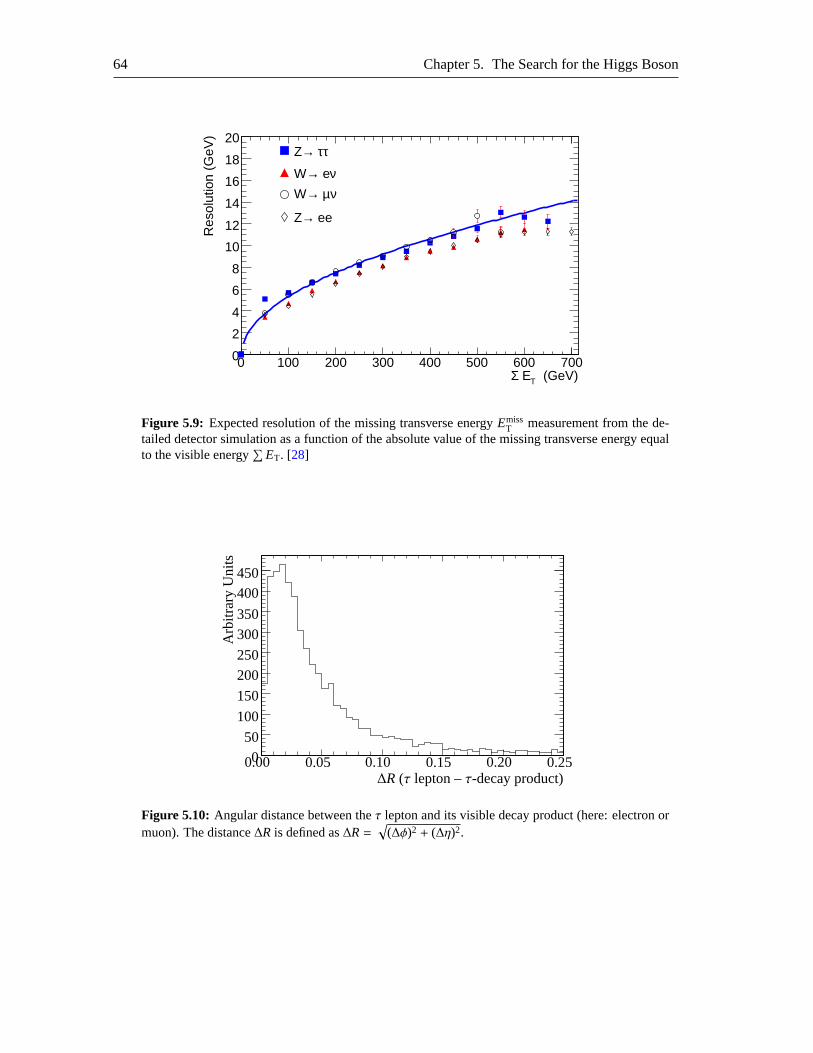
64 Chapter 5. The Search for the Higgs Boson
(GeV)T EΣ0 100 200 300 400 500 600 700
Res
olut
ion
(GeV
)
0
2
4
6
8
10
12
14
16
18
20ττ →Z
ν e→W
νµ →W
ee→Z
Figure 5.9: Expected resolution of the missing transverse energyEmissT measurement from the de-
tailed detector simulation as a function of the absolute value of the missing transverse energy equalto the visible energy
∑
ET. [28]
050
100
150
200250
300350
400450
0.00 0.05 0.10 0.15 0.20 0.25∆R (τ lepton –τ-decay product)
Arb
itrar
yU
nits
Figure 5.10: Angular distance between theτ lepton and its visible decay product (here: electron ormuon). The distance∆R is defined as∆R=
√
(∆φ)2 + (∆η)2.
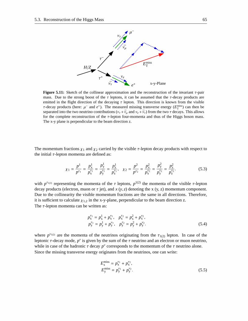
5.3. Reconstruction of the Higgs Mass 65
x-y-Plane
H/Z
τ+
τ−
e+
µ−
EmissT
νe
ντ
νµ
ντ
Figure 5.11: Sketch of the collinear approximation and the reconstruction of the invariantτ-pairmass. Due to the strong boost of theτ leptons, it can be assumed that theτ-decay products areemitted in the flight direction of the decayingτ lepton. This direction is known from the visibleτ-decay products (here:µ− ande+). The measured missing transverse energy (Emiss
T ) can then beseparated into the two neutrino contributions (ντ+ νµ andνe+ ντ) from the twoτ decays. This allowsfor the complete reconstruction of theτ-lepton four-momenta and thus of the Higgs boson mass.The x-y plane is perpendicular to the beam direction z.
The momentum fractionsχ1 andχ2 carried by the visibleτ-lepton decay products with respect tothe initialτ-lepton momenta are defined as:
χ1 =p1
pτ1=
p1x
pτ1x=
p1y
pτ1y=
p1z
pτ1z, χ2 =
p2
pτ2=
p2x
pτ2x=
p2y
pτ2y=
p2z
pτ2z. (5.3)
with pτ1(2) representing the momenta of theτ leptons,p1(2) the momenta of the visibleτ-leptondecay products (electron, muon orτ jet), andx (y, z) denoting the x (y, z) momentum component.Due to the collinearity the visible momentum fractions are the same in all directions. Therefore,it is sufficient to calculateχ1,2 in the x-y-plane, perpendicular to the beam direction z.Theτ-lepton momenta can be written as:
pτ1x = p1x + pν1x , pτ2x = p2
x + pν2x ,
pτ1y = p1y + pν1y , pτ2y = p2
y + pν2y . (5.4)
where pν1(2) are the momenta of the neutrinos originating from theτ1(2) lepton. In case of theleptonicτ-decay mode,pν is given by the sum of theτ neutrino and an electron or muon neutrino,while in case of the hadronicτ decaypν corresponds to the momentum of theτ neutrino alone.Since the missing transverse energy originates from the neutrinos, one can write:
Emissx = pν1x + pν2x ,
Emissy = pν1y + pν2y . (5.5)

66 Chapter 5. The Search for the Higgs Boson
Using equations5.3and5.4this can be written as:
Emissx = p1
x1− χ1
χ1+ p2
x1− χ2
χ2
Emissy = p1
y1− χ1
χ1+ p2
y1− χ2
χ2(5.6)
Solving this system of equations one obtains:
χ1 =p1
x p2y − p1
y p2x
p2y(p1
x + Emissx ) − p2
x(p1y + Emiss
y )
χ2 =p1
x p2y − p1
y p2x
p1x(p2
y + Emissy ) − p1
y(p2x + Emiss
x )(5.7)
Thus, the momentum fractionsχ1 andχ2 of the visibleτ-decay products can be calculated andthe momentum of the decayingτ lepton can be evaluated according to equation5.3. Knowing themomenta of theτ leptons it is now possible to calculate the Higgs massmH by determining theinvariant massmττ of theτ-lepton pair:
mH = mττ =√
(Pτ1 + Pτ2)2 (5.8)
The mass of theτ leptons can be neglected because of their high momenta, leading to:
mH =√
2pτ1 pτ2 · (1− cos(∆φττ) (5.9)
where∆φττ is the angle between the twoτ leptons (or, due to the collinear approximation, betweenthe two visibleτ-decay products).Since theZ decay intoτ leptons is very similar to the signal and as theZ boson (mZ = 91.2 GeV [22])is also much heavier than aτ lepton, the collinear approximation can also be used to reconstructtheZ mass.
Limitation of the Collinear Approximation In case of the leptons being emitted back-to-back,the previously mentioned system of equations (5.7) does not have a unique solution and the sepa-ration of the total transverse missing energy into the two neutrino contributionsis ambiguous.For leptons that are back-to-back in the r-φ plane one can write:
p2x = −a · p1
x
p2y = −a · p1
y , (5.10)
wherea is an arbitrary constant greater than zero.Inserting this into equations5.7, the numerators of the equations are zero and the calculation ofthe τ-lepton momentum with equation5.3 results in a singularity. Therefore, the application ofthe collinear approximation is limited to the cases where the twoτ-decay products are not back-to-back. This is usually ensured by requiring the angular separation of theτ-decay products,∆φττto be smaller than 180◦.
5.4. Event Selection Criteria 67
Performance of the Collinear Approximation The invariant Higgs mass resulting from thecollinear approximation is shown in Figure5.12afor a simulated Higgs mass of 120 GeV where theintrinsic width of the generated Higgs resonance can be neglected. The distribution is obtained us-ing the generated four-momenta of the visibleτ-decay products without additional, detector relatedeffects. The mass peak can be fitted with a Gauss function with a mean ofµ = (119.5± 0.1) GeVand a standard deviation ofσ = (3.0± 0.1) GeV.
Figure 5.12bshows the impact of the detector performance on the reconstructed Higgs bosonmass. The detector response leads to a shift of the mean mass value toµ = (118.0± 0.2) GeVand to a broadening of the width toσ = (10.3± 0.2) GeV. It can be seen that the main sourceof the degraded mass resolution is the resolution of the missing energy measurement. The finiteresolution of the missing transverse energy measurement broadens the mass distribution even morethan the collinear approximation itself assuming an exactly knownEmiss
T . In contrast to this, thelepton momentum resolution has a negligible effect on the reconstructed invariant mass. This canbe expected since the resolution of the momentum measurement of electrons and muons is in theorder of 2-3 % while it is only∼10 % for the missing transverse energy measurement. A wellunderstood and precise reconstruction of the missing transverse energy is therefore crucial for theHiggs boson discovery in this channel.The expected ATLAS detector performance allows for a good separationof theZ resonance andthe Higgs signal peak for Higgs masses above&110 GeV.
5.4 Event Selection Criteria
In order to suppress background processes in the presented Higgs boson search channel, a varietyof selection criteria are available which are introduced in the following. The criteria can be dividedinto three categories: one group related to theτ-decay products, another group concerning theforward jets produced in the vector-boson fusion and a last group related to both parts of an event,theτ-decay products and the forward jets.For several reasons, the selection cuts on some discriminating variables have been fixed to a certainvalue or constrained to a subrange of the distribution (preselection). Forthese variables, the cutvalue is shown in the following distributions and the motivation for the cut is explained in the text.If no cut is indicated in the figure, no obvious reason for a certain cut value exists and the cut onthe variable has been optimized as described in Chapter6 or has been used as an input variable tomultivariate analysis methods (see Chapter7).
5.4.1 τ-Decay Products Criteria
Trigger
As a first step in each analysis, it is inevitable to require an event to be accepted by the triggeralgorithm. In the leptonic and semileptonicH → ττ channel, there is at least one electron or muonamong the decay products in the final state. Therefore, the signal eventscan be triggered by high-
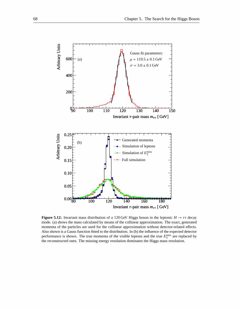
68 Chapter 5. The Search for the Higgs Boson
009090 100100 110110 120120 130130 140140 150150
200200
400400
600600A
rbitr
ary
Uni
tsA
rbitr
ary
Uni
ts
Invariantτ-pair massmττ [ GeV]Invariantτ-pair massmττ [ GeV]
(a)
Gauss fit parameters:
σ = 3.0± 0.1 GeV
µ = 119.5± 0.1 GeV
8080 100100 120120 140140 160160 1801800.000.00
0.050.05
0.100.10
0.150.15
0.200.20
0.250.25
Arb
itrar
yU
nits
Arb
itrar
yU
nits
Generated momenta
Simulation of leptons
Simulation ofEmissT
Full simulation
Invariantτ-pair massmττ [ GeV]Invariantτ-pair massmττ [ GeV]
(b)
Figure 5.12: Invariant mass distribution of a 120 GeV Higgs boson in the leptonic H → ττ decaymode. (a) shows the mass calculated by means of the collinearapproximation. The exact, generatedmomenta of the particles are used for the collinear approximation without detector-related effects.Also shown is a Gauss function fitted to the distribution. In (b) the influence of the expected detectorperformance is shown. The true momenta of the visible leptons and the trueEmiss
T are replaced bythe reconstructed ones. The missing energy resolution dominates the Higgs mass resolution.
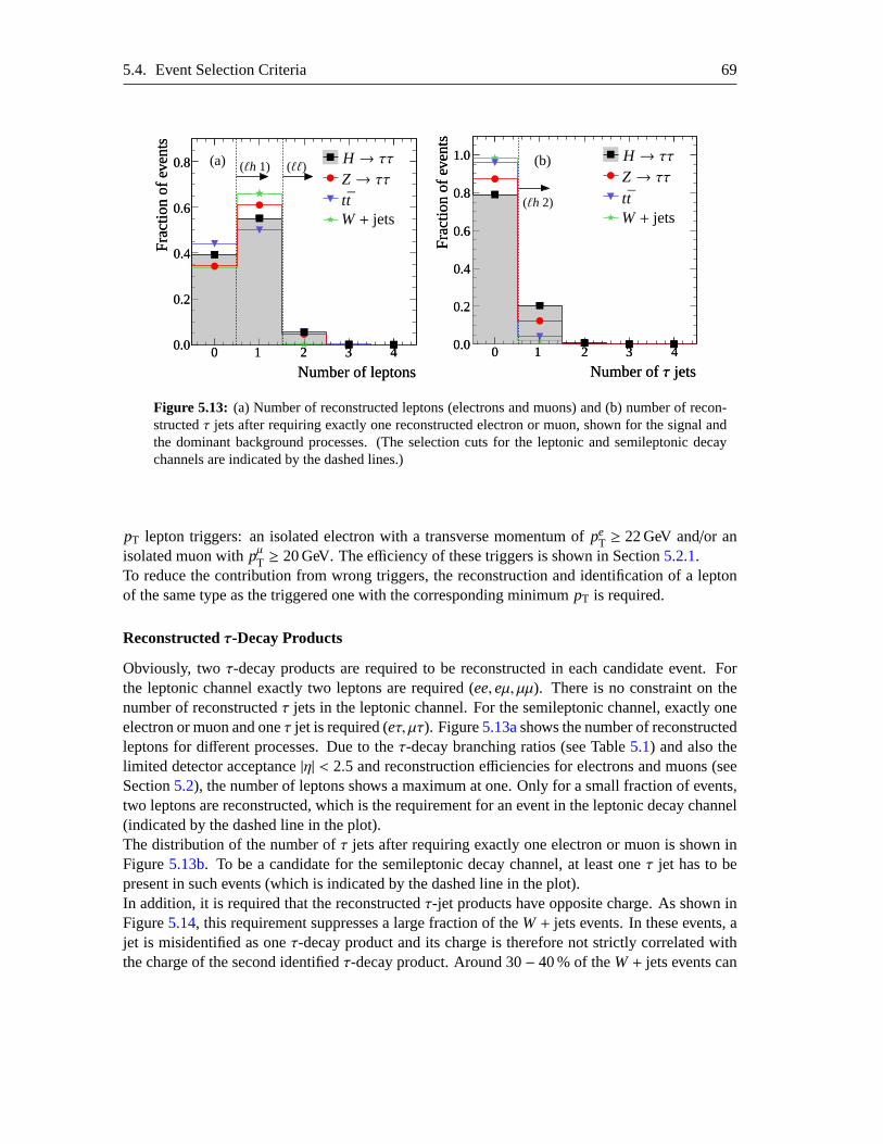
5.4. Event Selection Criteria 69
00 11 22 33 440.00.0
0.20.2
0.40.4
0.60.6
0.80.8Z→ ττH → ττ
ttW+ jets
Number of leptonsNumber of leptons
Fra
ctio
nof
even
tsF
ract
ion
ofev
ents
(a) (ℓh 1) (ℓℓ)
00 11 22 33 440.00.0
0.20.2
0.40.4
0.60.6
0.80.8
1.01.0
Z→ ττH → ττ
ttW+ jets
Number ofτ jetsNumber ofτ jets
Fra
ctio
nof
even
tsF
ract
ion
ofev
ents
(b)
(ℓh 2)
Figure 5.13: (a) Number of reconstructed leptons (electrons and muons) and (b) number of recon-structedτ jets after requiring exactly one reconstructed electron ormuon, shown for the signal andthe dominant background processes. (The selection cuts forthe leptonic and semileptonic decaychannels are indicated by the dashed lines.)
pT lepton triggers: an isolated electron with a transverse momentum ofpeT ≥ 22 GeV and/or an
isolated muon withpµT ≥ 20 GeV. The efficiency of these triggers is shown in Section5.2.1.To reduce the contribution from wrong triggers, the reconstruction and identification of a leptonof the same type as the triggered one with the corresponding minimumpT is required.
Reconstructedτ-Decay Products
Obviously, twoτ-decay products are required to be reconstructed in each candidate event. Forthe leptonic channel exactly two leptons are required (ee,eµ, µµ). There is no constraint on thenumber of reconstructedτ jets in the leptonic channel. For the semileptonic channel, exactly oneelectron or muon and oneτ jet is required (eτ, µτ). Figure5.13ashows the number of reconstructedleptons for different processes. Due to theτ-decay branching ratios (see Table5.1) and also thelimited detector acceptance|η| < 2.5 and reconstruction efficiencies for electrons and muons (seeSection5.2), the number of leptons shows a maximum at one. Only for a small fraction of events,two leptons are reconstructed, which is the requirement for an event in theleptonic decay channel(indicated by the dashed line in the plot).The distribution of the number ofτ jets after requiring exactly one electron or muon is shown inFigure5.13b. To be a candidate for the semileptonic decay channel, at least oneτ jet has to bepresent in such events (which is indicated by the dashed line in the plot).In addition, it is required that the reconstructedτ-jet products have opposite charge. As shown inFigure5.14, this requirement suppresses a large fraction of theW+ jets events. In these events, ajet is misidentified as oneτ-decay product and its charge is therefore not strictly correlated withthe charge of the second identifiedτ-decay product. Around 30− 40 % of theW+ jets events can
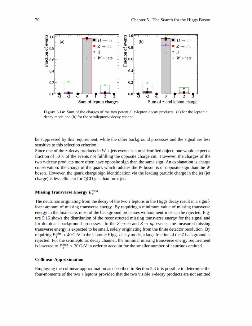
70 Chapter 5. The Search for the Higgs Boson
-3-3 -2-2 -1-1 00 11 22 330.00.0
0.20.2
0.40.4
0.60.6
0.80.8
1.01.0
j j
Z→ ττH → ττ
ttW+ jets
Sum of lepton chargesSum of lepton charges
Fra
ctio
nof
even
tsF
ract
ion
ofev
ents
(a)
-3-3 -2-2 -1-1 00 11 22 330.00.0
0.20.2
0.40.4
0.60.6
0.80.8
1.01.0
Z→ ττH → ττ
ttW+ jets
Sum ofτ and lepton chargeSum ofτ and lepton charge
Fra
ctio
nof
even
tsF
ract
ion
ofev
ents
(b)
Figure 5.14: Sum of the charges of the two potentialτ-lepton decay products. (a) for the leptonicdecay mode and (b) for the semileptonic decay channel.
be suppressed by this requirement, while the other background processes and the signal are lesssensitive to this selection criterion.Since one of theτ-decay products inW+ jets events is a misidentified object, one would expect afraction of 50 % of the events not fulfilling the opposite charge cut. However, the charges of thetwo τ-decay products more often have opposite sign than the same sign. An explanation is chargeconservation: the charge of the quark which radiates theW boson is of opposite sign than theWboson. However, the quark charge sign identification via the leading particle charge in the jet (jetcharge) is less efficient for QCD jets than forτ jets.
Missing Transverse EnergyEmissT
The neutrinos originating from the decay of the twoτ leptons in the Higgs decay result in a signif-icant amount of missing transverse energy. By requiring a minimum value of missing transverseenergy in the final state, most of the background processes without neutrinos can be rejected. Fig-ure5.15shows the distribution of the reconstructed missing transverse energy forthe signal andfor dominant background processes. In theZ→ eeandZ→ µµ events, the measured missingtransverse energy is expected to be small, solely originating from the finite detector resolution. ByrequiringEmiss
T > 40 GeV in the leptonic Higgs decay mode, a large fraction of theZ background isrejected. For the semileptonic decay channel, the minimal missing transverse energy requirementis lowered toEmiss
T > 30 GeV in order to account for the smaller number of neutrinos emitted.
Collinear Approximation
Employing the collinear approximation as described in Section5.3 it is possible to determine thefour-momenta of the twoτ leptons provided that the two visibleτ-decay products are not emitted
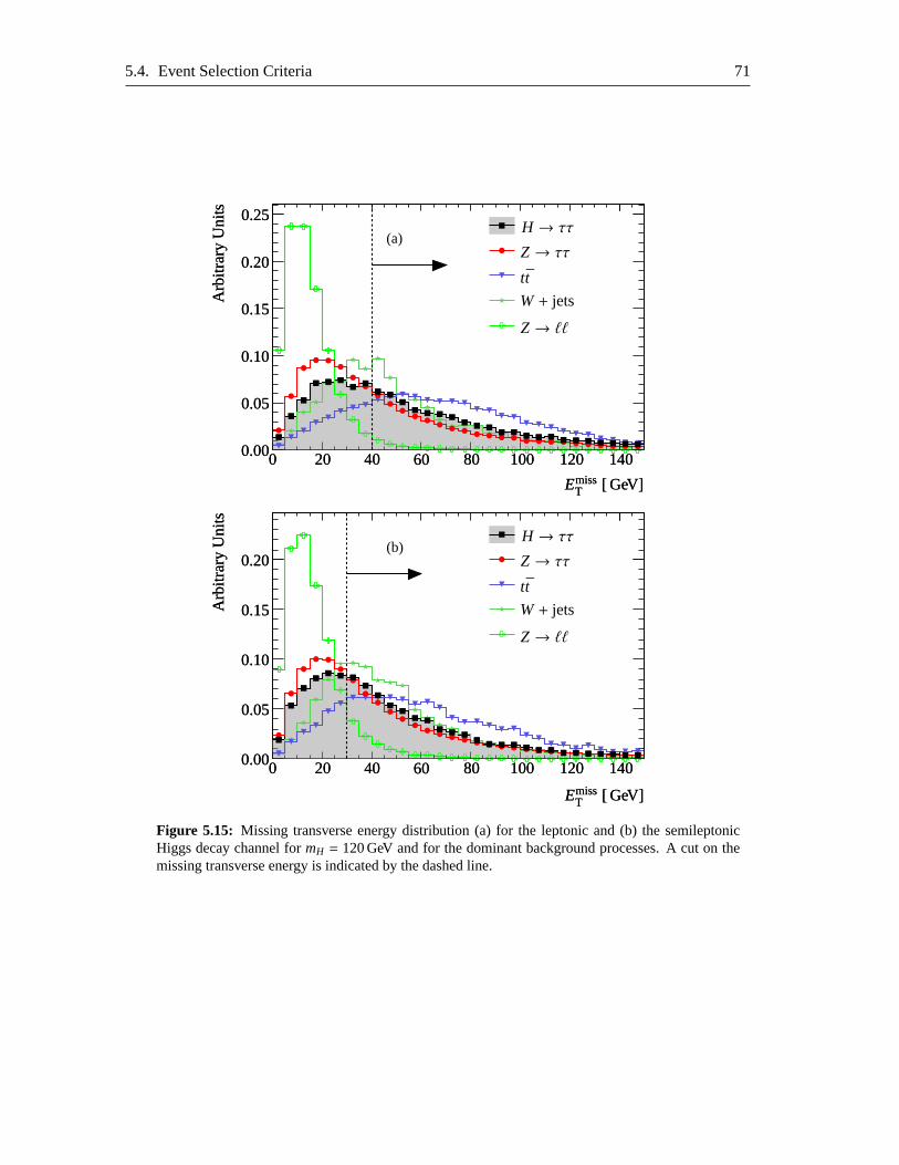
5.4. Event Selection Criteria 71
00 2020 4040 6060 8080 100100 120120 1401400.000.00
0.050.05
0.100.10
0.150.15
0.200.20
0.250.25A
rbitr
ary
Uni
tsA
rbitr
ary
Uni
ts
Fraction
EmissT [ GeV]EmissT [ GeV]
Z→ ττH → ττ
Z→ ℓℓ
tt
W+ jets
(a)
00 2020 4040 6060 8080 100100 120120 1401400.000.00
0.050.05
0.100.10
0.150.15
0.200.20
Arb
itrar
yU
nits
Arb
itrar
yU
nits
EmissT [ GeV]EmissT [ GeV]
Z→ ττH → ττ
Z→ ℓℓ
tt
W+ jets
(b)
Figure 5.15: Missing transverse energy distribution (a) for the leptonic and (b) the semileptonicHiggs decay channel formH = 120 GeV and for the dominant background processes. A cut on themissing transverse energy is indicated by the dashed line.
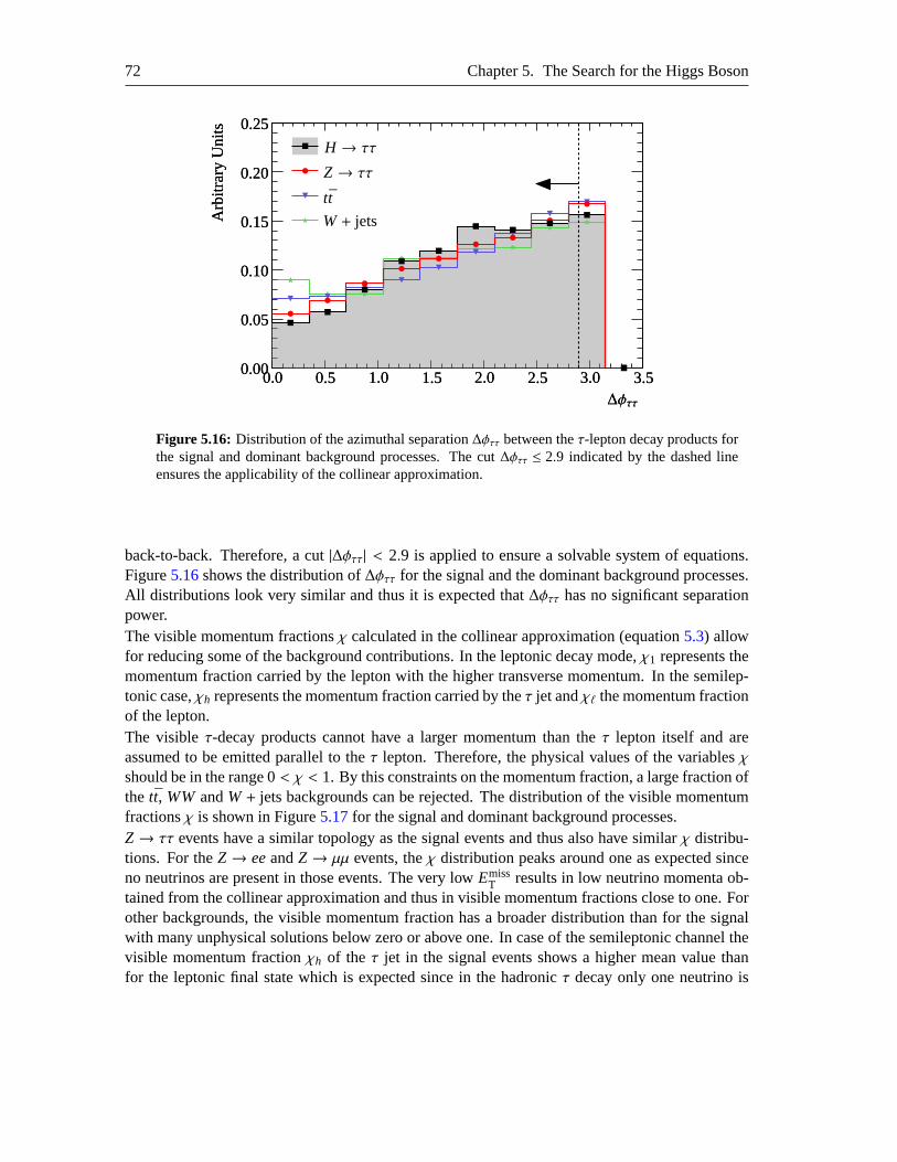
72 Chapter 5. The Search for the Higgs Boson
0.00.0 0.50.5 1.01.0 1.51.5 2.02.0 2.52.5 3.03.0 3.53.50.000.00
0.050.05
0.100.10
0.150.15
0.200.20
0.250.25
Arb
itrar
yU
nits
Arb
itrar
yU
nits
Z→ ττH → ττ
tt
W+ jets
∆φττ∆φττ
Figure 5.16: Distribution of the azimuthal separation∆φττ between theτ-lepton decay products forthe signal and dominant background processes. The cut∆φττ ≤ 2.9 indicated by the dashed lineensures the applicability of the collinear approximation.
back-to-back. Therefore, a cut|∆φττ| < 2.9 is applied to ensure a solvable system of equations.Figure5.16shows the distribution of∆φττ for the signal and the dominant background processes.All distributions look very similar and thus it is expected that∆φττ has no significant separationpower.The visible momentum fractionsχ calculated in the collinear approximation (equation5.3) allowfor reducing some of the background contributions. In the leptonic decaymode,χ1 represents themomentum fraction carried by the lepton with the higher transverse momentum. In the semilep-tonic case,χh represents the momentum fraction carried by theτ jet andχℓ the momentum fractionof the lepton.The visibleτ-decay products cannot have a larger momentum than theτ lepton itself and areassumed to be emitted parallel to theτ lepton. Therefore, the physical values of the variablesχshould be in the range 0< χ < 1. By this constraints on the momentum fraction, a large fraction ofthe tt, WWandW+ jets backgrounds can be rejected. The distribution of the visible momentumfractionsχ is shown in Figure5.17for the signal and dominant background processes.Z→ ττ events have a similar topology as the signal events and thus also have similarχ distribu-tions. For theZ→ eeandZ→ µµ events, theχ distribution peaks around one as expected sinceno neutrinos are present in those events. The very lowEmiss
T results in low neutrino momenta ob-tained from the collinear approximation and thus in visible momentum fractions close to one. Forother backgrounds, the visible momentum fraction has a broader distributionthan for the signalwith many unphysical solutions below zero or above one. In case of the semileptonic channel thevisible momentum fractionχh of the τ jet in the signal events shows a higher mean value thanfor the leptonic final state which is expected since in the hadronicτ decay only one neutrino is
5.4. Event Selection Criteria 73
emitted.The differences between the signal and the different background processes are even more pro-nounced in the two-dimensionalχ1,2 distributions as shown in Figure5.19.
Transverse Mass
The invariant mass of the transverse components of one lepton momentum andof the missingtransverse energy, the transverse massmℓνT , is given by:
mℓνT =√
2pTℓEmiss
T · (1− cos∆φ). (5.11)
In the leptonic decay mode,pTℓ is from the lepton (electron or muon) with the higher transverse
momentumpT. In the semileptonic decay mode,pTℓ is the transverse momentum of the electron
or muon. The angle∆φ is the azimuthal angle between the lepton and the missing transverse en-ergy. The distribution of the transverse mass is shown in Figure5.20. For theW+ jets events,the calculated mass value corresponds to the transverse component of theW boson mass. Onecan see that theW+ jets events have a higher transverse mass than the signal or the other back-ground processes excepttt, with the trailing edge of the distribution close to theW boson mass(80.4 GeV [22]).Therefore, requiring the transverse mass to be less than 30 GeV helps to suppress mainly theW+ jets background, but also a large fraction of thett events is discarded. This discriminat-ing variable is particularly important for the semileptonic decay mode where it helps to suppressW+ jets events in which theW boson decays leptonically with additional QCD radiation faking aτ jet. In the leptonic decay mode, theW+ jets background is much less important and, thus, thecut onmℓνT can be looser.
5.4.2 Tagging Jets Criteria
Tagging Jet Candidates
The presence of at least two reconstructed jets in the final state is required to account for thevector-boson fusion signature with two jets in the forward region of the detector. The number ofreconstructed jets withpT > 20 GeV is shown in Figure5.21.In contrast to the highpT jets of the vector-boson fusion process, jets produced by QCD processeshave a steeply fallingpT distribution. In order to suppressW andZ events which contain QCD jetsit is required that at least one of the two jets has a minimum transverse momentum of pT > 40 GeV.The two jets with the highestpT are considered as candidates for the tagging jets. Since in thevector-boson fusion process the jets are mainly produced in opposite hemispheres of the detector,all events containing these two jets in the same hemisphere are rejected.
Tagging Jet Kinematics
The two jets produced in the vector-boson fusion process typically have alarge rapidity gap (∆η j j )and high energy and thus a large invariant mass (mj j ). In contrast, jets from QCD processes aremore located in the central region of the detector. Figure5.22ashows the distribution of the
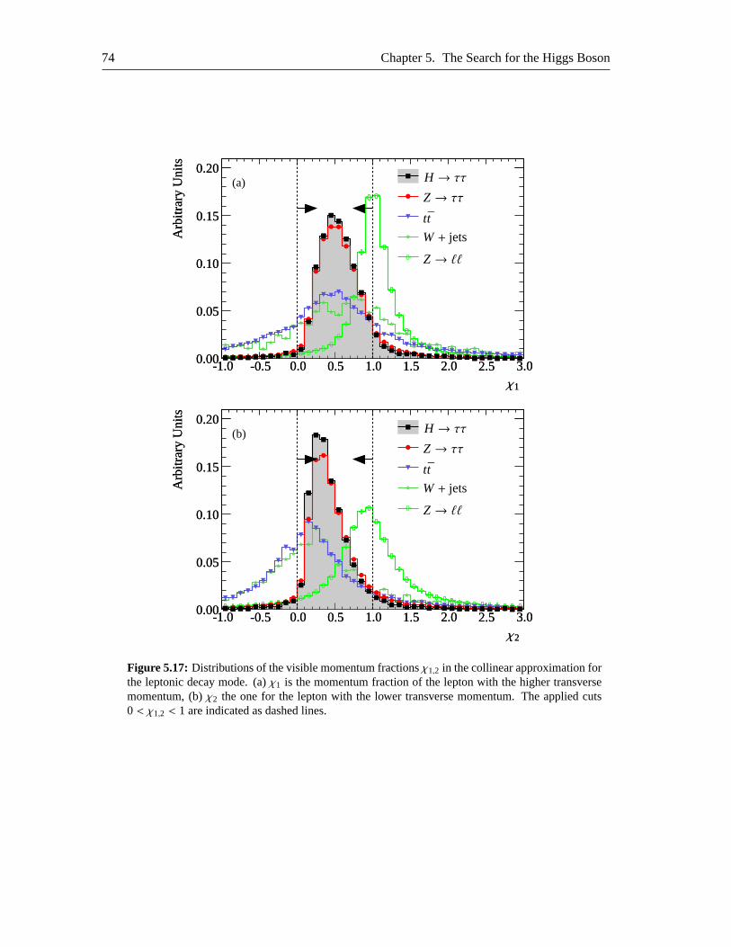
74 Chapter 5. The Search for the Higgs Boson
-1.0-1.0 -0.5-0.5 0.00.0 0.50.5 1.01.0 1.51.5 2.02.0 2.52.5 3.03.00.000.00
0.050.05
0.100.10
0.150.15
0.200.20A
rbitr
ary
Uni
tsA
rbitr
ary
Uni
ts
Z→ ττH → ττ
Z→ ℓℓ
tt
W+ jets
χ1χ1
(a)
-1.0-1.0 -0.5-0.5 0.00.0 0.50.5 1.01.0 1.51.5 2.02.0 2.52.5 3.03.00.000.00
0.050.05
0.100.10
0.150.15
0.200.20
Arb
itrar
yU
nits
Arb
itrar
yU
nits
Z→ ττH → ττ
Z→ ℓℓ
tt
W+ jets
χ2χ2
(b)
Figure 5.17: Distributions of the visible momentum fractionsχ1,2 in the collinear approximation forthe leptonic decay mode. (a)χ1 is the momentum fraction of the lepton with the higher transversemomentum, (b)χ2 the one for the lepton with the lower transverse momentum. The applied cuts0 < χ1,2 < 1 are indicated as dashed lines.
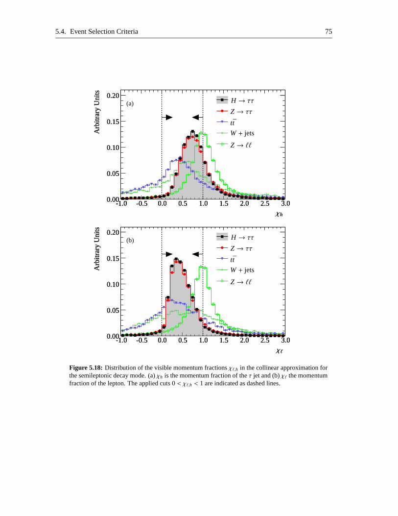
5.4. Event Selection Criteria 75
-1.0-1.0 -0.5-0.5 0.00.0 0.50.5 1.01.0 1.51.5 2.02.0 2.52.5 3.03.00.000.00
0.050.05
0.100.10
0.150.15
0.200.20A
rbitr
ary
Uni
tsA
rbitr
ary
Uni
ts
Z→ ττH → ττ
Z→ ℓℓ
tt
W+ jets
χhχh
(a)
-1.0-1.0 -0.5-0.5 0.00.0 0.50.5 1.01.0 1.51.5 2.02.0 2.52.5 3.03.00.000.00
0.050.05
0.100.10
0.150.15
0.200.20
Arb
itrar
yU
nits
Arb
itrar
yU
nits
Z→ ττH → ττ
Z→ ℓℓ
tt
W+ jets
χℓχℓ
(b)
Figure 5.18: Distribution of the visible momentum fractionsχℓ,h in the collinear approximation forthe semileptonic decay mode. (a)χh is the momentum fraction of theτ jet and (b)χℓ the momentumfraction of the lepton. The applied cuts 0< χℓ,h < 1 are indicated as dashed lines.
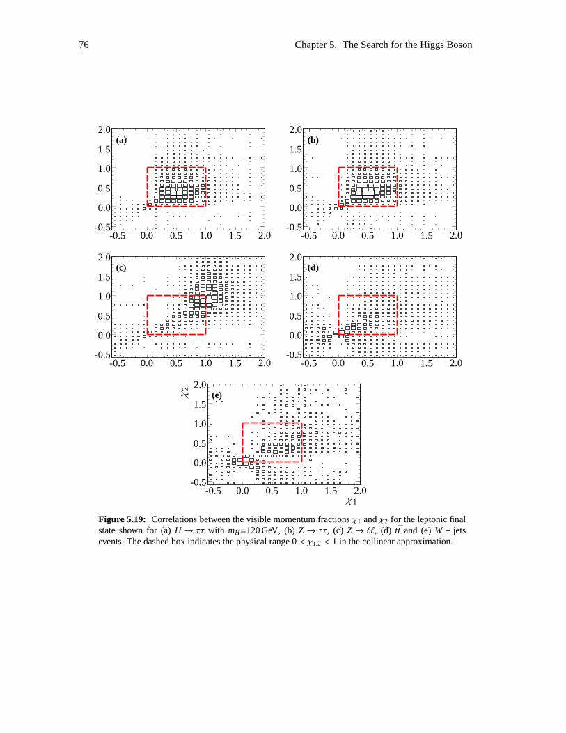
76 Chapter 5. The Search for the Higgs Boson
-0.5-0.5
0.0
0.0
0.5
0.5
1.0
1.0
1.5
1.5
2.0
2.0
∆
(a)
-0.5-0.5
0.0
0.0
0.5
0.5
1.0
1.0
1.5
1.5
2.0
2.0
(b)
-0.5-0.5
0.0
0.0
0.5
0.5
1.0
1.0
1.5
1.5
2.0
2.0
0.45
(c)
-0.5-0.5
0.0
0.0
0.5
0.5
1.0
1.0
1.5
1.5
2.0
2.0
(d)
-0.5-0.5
0.0
0.0
0.5
0.5
1.0
1.0
1.5
1.5
2.0
2.0χ1
χ2
(e)
Figure 5.19: Correlations between the visible momentum fractionsχ1 andχ2 for the leptonic finalstate shown for (a)H → ττ with mH=120 GeV, (b)Z→ ττ, (c) Z→ ℓℓ, (d) tt and (e)W+ jetsevents. The dashed box indicates the physical range 0< χ1,2 < 1 in the collinear approximation.
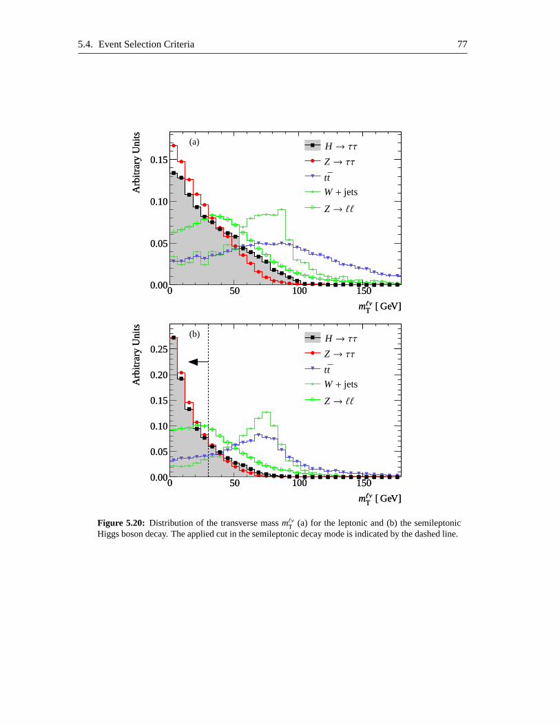
5.4. Event Selection Criteria 77
00 5050 100100 1501500.000.00
0.050.05
0.100.10
0.150.15
Arb
itrar
yU
nits
Arb
itrar
yU
nits
Z→ ττH → ττ
Z→ ℓℓ
tt
W+ jets
mℓνT [ GeV]mℓνT [ GeV]
(a)
00 5050 100100 1501500.000.00
0.050.05
0.100.10
0.150.15
0.200.20
0.250.25
Arb
itrar
yU
nits
Arb
itrar
yU
nits
Z→ ττH → ττ
Z→ ℓℓ
tt
W+ jets
mℓνT [ GeV]mℓνT [ GeV]
(b)
Figure 5.20: Distribution of the transverse massmℓνT (a) for the leptonic and (b) the semileptonicHiggs boson decay. The applied cut in the semileptonic decaymode is indicated by the dashed line.
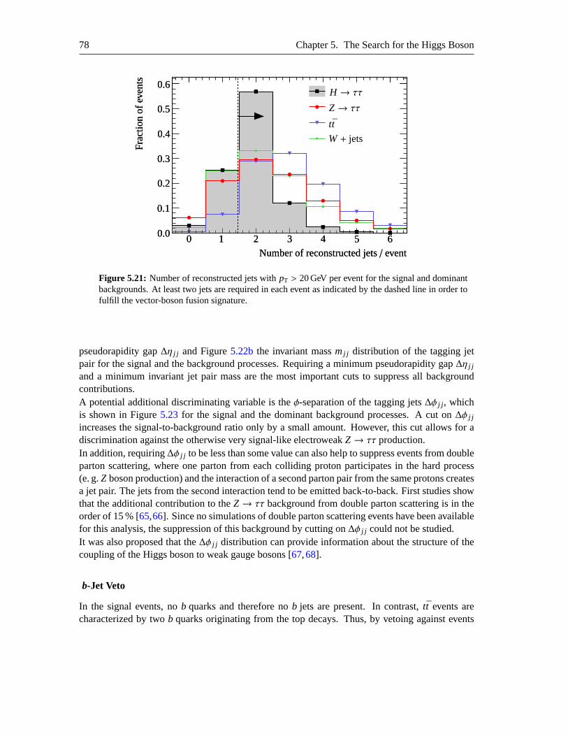
78 Chapter 5. The Search for the Higgs Boson
00 11 22 33 44 55 660.00.0
0.10.1
0.20.2
0.30.3
0.40.4
0.50.5
0.60.6
Fra
ctio
nof
even
tsF
ract
ion
ofev
ents
Z→ ττH → ττ
tt
W+ jets
Number of reconstructed jets/ eventNumber of reconstructed jets/ event
Figure 5.21: Number of reconstructed jets withpT > 20 GeV per event for the signal and dominantbackgrounds. At least two jets are required in each event as indicated by the dashed line in order tofulfill the vector-boson fusion signature.
pseudorapidity gap∆η j j and Figure5.22bthe invariant massmj j distribution of the tagging jetpair for the signal and the background processes. Requiring a minimum pseudorapidity gap∆η j j
and a minimum invariant jet pair mass are the most important cuts to suppress all backgroundcontributions.A potential additional discriminating variable is theφ-separation of the tagging jets∆φ j j , whichis shown in Figure5.23 for the signal and the dominant background processes. A cut on∆φ j j
increases the signal-to-background ratio only by a small amount. However, this cut allows for adiscrimination against the otherwise very signal-like electroweakZ→ ττ production.In addition, requiring∆φ j j to be less than some value can also help to suppress events from doubleparton scattering, where one parton from each colliding proton participates in the hard process(e. g.Z boson production) and the interaction of a second parton pair from the same protons createsa jet pair. The jets from the second interaction tend to be emitted back-to-back. First studies showthat the additional contribution to theZ→ ττ background from double parton scattering is in theorder of 15 % [65,66]. Since no simulations of double parton scattering events have been availablefor this analysis, the suppression of this background by cutting on∆φ j j could not be studied.It was also proposed that the∆φ j j distribution can provide information about the structure of thecoupling of the Higgs boson to weak gauge bosons [67,68].
b-Jet Veto
In the signal events, nob quarks and therefore nob jets are present. In contrast,tt events arecharacterized by twob quarks originating from the top decays. Thus, by vetoing against events
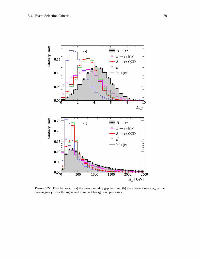
5.4. Event Selection Criteria 79
00 22 44 66 88 10100.000.00
0.050.05
0.100.10
0.150.15
Arb
itrar
yU
nits
Arb
itrar
yU
nits
Fraction
∆η j j∆η j j
Z→ ττ QCD
Z→ ττ EW
H → ττ
tt
W+ jets
(a)
00 500500 10001000 15001500 20002000 250025000.000.00
0.050.05
0.100.10
0.150.15
0.200.20
0.250.25
Arb
itrar
yU
nits
Arb
itrar
yU
nits
mj j [ GeV]mj j [ GeV]
Z→ ττ QCD
Z→ ττ EW
H → ττ
tt
W+ jets
(b)
Figure 5.22: Distributions of (a) the pseudorapidity gap∆η j j and (b) the invariant massmj j of thetwo tagging jets for the signal and dominant background processes.
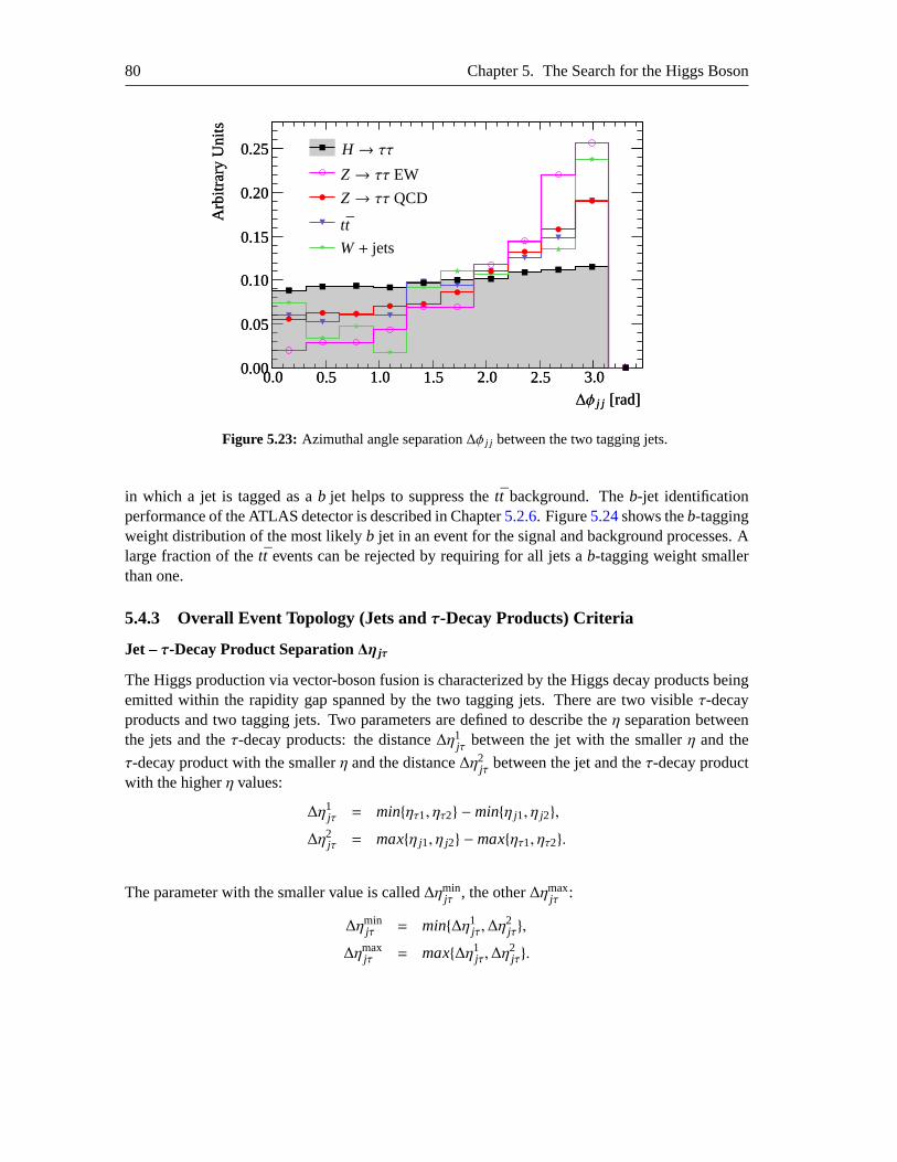
80 Chapter 5. The Search for the Higgs Boson
0.00.0 0.50.5 1.01.0 1.51.5 2.02.0 2.52.5 3.03.00.000.00
0.050.05
0.100.10
0.150.15
0.200.20
0.250.25
Arb
itrar
yU
nits
Arb
itrar
yU
nits
Z→ ττ QCD
Z→ ττ EW
H → ττ
tt
W+ jets
∆φ j j [rad]∆φ j j [rad]
Figure 5.23: Azimuthal angle separation∆φ j j between the two tagging jets.
in which a jet is tagged as ab jet helps to suppress thett background. Theb-jet identificationperformance of the ATLAS detector is described in Chapter5.2.6. Figure5.24shows theb-taggingweight distribution of the most likelyb jet in an event for the signal and background processes. Alarge fraction of thett events can be rejected by requiring for all jets ab-tagging weight smallerthan one.
5.4.3 Overall Event Topology (Jets andτ-Decay Products) Criteria
Jet –τ-Decay Product Separation∆η jτ
The Higgs production via vector-boson fusion is characterized by the Higgs decay products beingemitted within the rapidity gap spanned by the two tagging jets. There are two visibleτ-decayproducts and two tagging jets. Two parameters are defined to describe theη separation betweenthe jets and theτ-decay products: the distance∆η1jτ between the jet with the smallerη and the
τ-decay product with the smallerη and the distance∆η2jτ between the jet and theτ-decay productwith the higherη values:
∆η1jτ = min{ητ1, ητ2} −min{η j1, η j2},∆η2jτ = max{η j1, η j2} −max{ητ1, ητ2}.
The parameter with the smaller value is called∆ηminjτ , the other∆ηmax
jτ :
∆ηminjτ = min{∆η1jτ,∆η
2jτ},
∆ηmaxjτ = max{∆η1jτ,∆η
2jτ}.
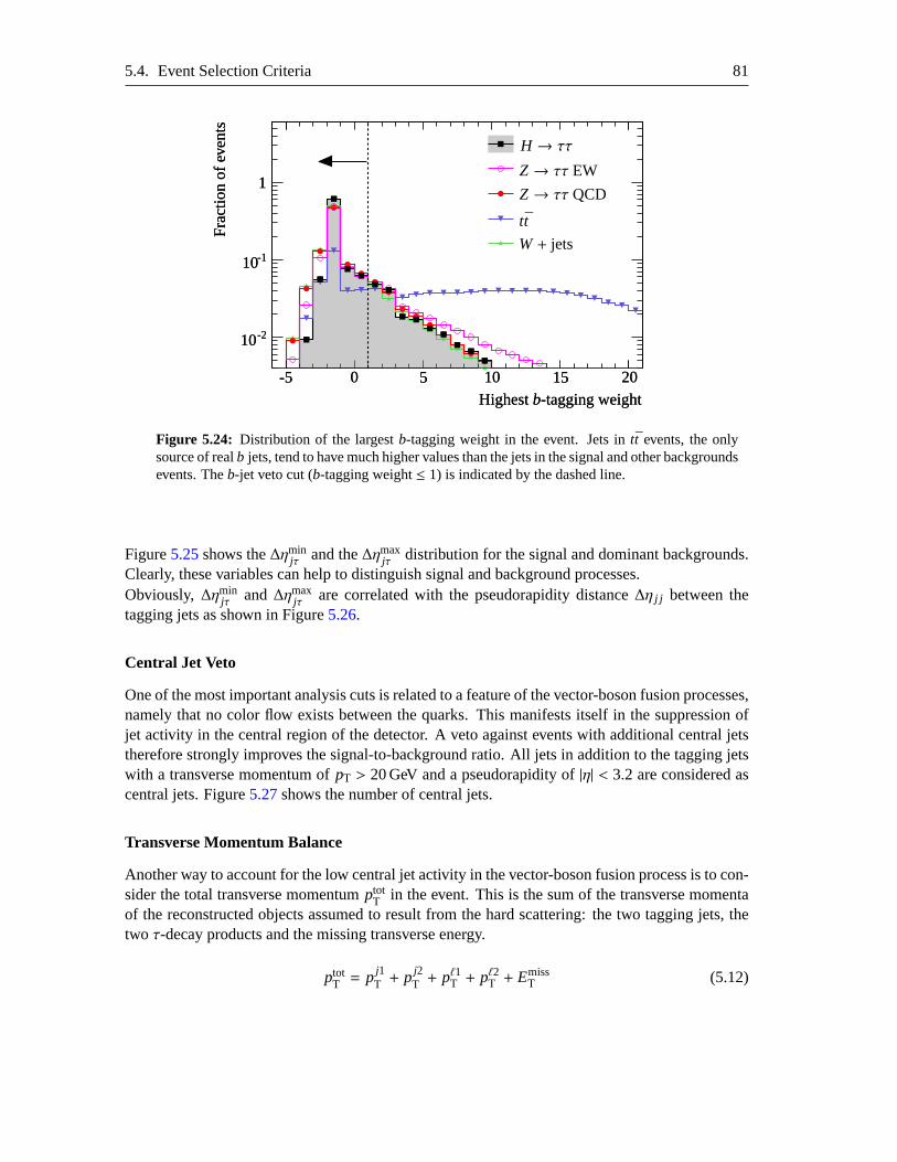
5.4. Event Selection Criteria 81
-5-5 00
11
55
10
10
10
10
10
10 1515 2020
Fra
ctio
nof
even
tsF
ract
ion
ofev
ents
Z→ ττ QCD
Z→ ττ EW
H → ττ
tt
W+ jets
Highestb-tagging weightHighestb-tagging weight
-1-1
-2-2
Figure 5.24: Distribution of the largestb-tagging weight in the event. Jets intt events, the onlysource of realb jets, tend to have much higher values than the jets in the signal and other backgroundsevents. Theb-jet veto cut (b-tagging weight≤ 1) is indicated by the dashed line.
Figure5.25shows the∆ηminjτ and the∆ηmax
jτ distribution for the signal and dominant backgrounds.Clearly, these variables can help to distinguish signal and background processes.Obviously,∆ηmin
jτ and∆ηmaxjτ are correlated with the pseudorapidity distance∆η j j between the
tagging jets as shown in Figure5.26.
Central Jet Veto
One of the most important analysis cuts is related to a feature of the vector-boson fusion processes,namely that no color flow exists between the quarks. This manifests itself in the suppression ofjet activity in the central region of the detector. A veto against events with additional central jetstherefore strongly improves the signal-to-background ratio. All jets in addition to the tagging jetswith a transverse momentum ofpT > 20 GeV and a pseudorapidity of|η| < 3.2 are considered ascentral jets. Figure5.27shows the number of central jets.
Transverse Momentum Balance
Another way to account for the low central jet activity in the vector-bosonfusion process is to con-sider the total transverse momentumptot
T in the event. This is the sum of the transverse momentaof the reconstructed objects assumed to result from the hard scattering: the two tagging jets, thetwo τ-decay products and the missing transverse energy.
ptotT = p j1
T + p j2T + pℓ1T + pℓ2T + Emiss
T (5.12)
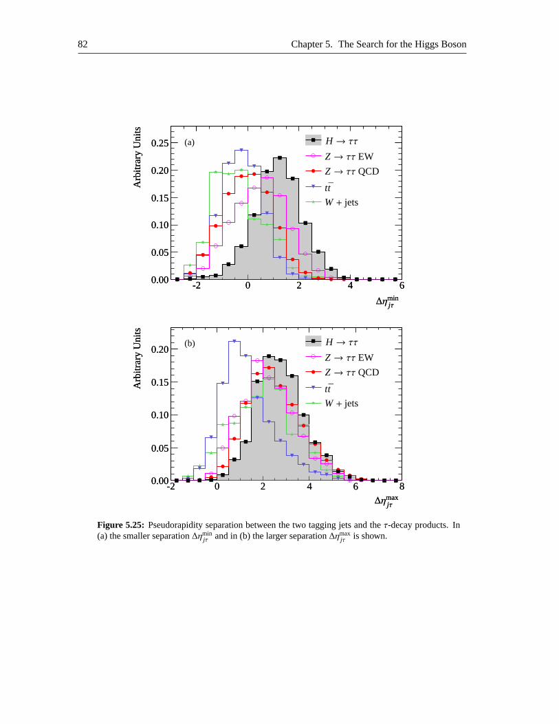
82 Chapter 5. The Search for the Higgs Boson
-2-2 00 22 44 660.000.00
0.050.05
0.100.10
0.150.15
0.200.20
0.250.25A
rbitr
ary
Uni
tsA
rbitr
ary
Uni
ts
Z→ ττ QCD
Z→ ττ EW
H → ττ
tt
W+ jets
∆ηminjτ∆ηminjτ
(a)
-2-2 00 22 44 66 880.000.00
0.050.05
0.100.10
0.150.15
0.200.20
Arb
itrar
yU
nits
Arb
itrar
yU
nits
Z→ ττ QCD
Z→ ττ EW
H → ττ
tt
W+ jets
∆ηmaxjτ∆ηmaxjτ
(b)
Figure 5.25: Pseudorapidity separation between the two tagging jets andtheτ-decay products. In(a) the smaller separation∆ηmin
jτ and in (b) the larger separation∆ηmaxjτ is shown.
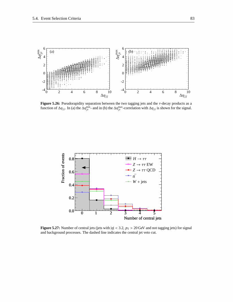
5.4. Event Selection Criteria 83
-4
-2
0
0
2
2
4
4
6
6 8 10
∆η
min
jτ
∆η
∆η j j
(a)
-4
-2
0
0
2
2
4
4
6
6 8 10
∆η
max
jτ
∆η j j
(b)
Figure 5.26: Pseudorapidity separation between the two tagging jets andtheτ-decay products as afunction of∆η j j . In (a) the∆ηmin
jτ - and in (b) the∆ηmaxjτ -correlation with∆η j j is shown for the signal.
00 11 22 33 44 550.00.0
0.20.2
0.40.4
0.60.6
0.80.8
Fra
ctio
nof
even
tsF
ract
ion
ofev
ents
Z→ ττ QCDZ→ ττ EW
H → ττ
ttW+ jets
Number of central jetsNumber of central jets
Figure 5.27: Number of central jets (jets with|η| < 3.2, pT > 20 GeV and not tagging jets) for signaland background processes. The dashed line indicates the central jet veto cut.
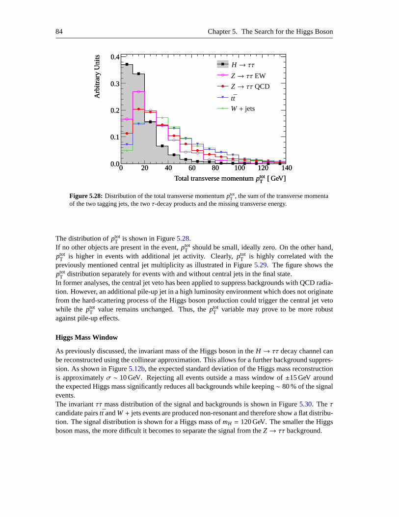
84 Chapter 5. The Search for the Higgs Boson
00 2020 4040 6060 8080 100100 120120 1401400.00.0
0.10.1
0.20.2
0.30.3
0.40.4
Arb
itrar
yU
nits
Arb
itrar
yU
nits
Z→ ττ QCD
Z→ ττ EW
H → ττ
tt
W+ jets
Total transverse momentumptotT [ GeV]Total transverse momentumptotT [ GeV]
Figure 5.28: Distribution of the total transverse momentumptotT , the sum of the transverse momenta
of the two tagging jets, the twoτ-decay products and the missing transverse energy.
The distribution ofptotT is shown in Figure5.28.
If no other objects are present in the event,ptotT should be small, ideally zero. On the other hand,
ptotT is higher in events with additional jet activity. Clearly,ptot
T is highly correlated with thepreviously mentioned central jet multiplicity as illustrated in Figure5.29. The figure shows theptot
T distribution separately for events with and without central jets in the final state.In former analyses, the central jet veto has been applied to suppress backgrounds with QCD radia-tion. However, an additional pile-up jet in a high luminosity environment which does not originatefrom the hard-scattering process of the Higgs boson production could trigger the central jet vetowhile the ptot
T value remains unchanged. Thus, theptotT variable may prove to be more robust
against pile-up effects.
Higgs Mass Window
As previously discussed, the invariant mass of the Higgs boson in theH → ττ decay channel canbe reconstructed using the collinear approximation. This allows for a further background suppres-sion. As shown in Figure5.12b, the expected standard deviation of the Higgs mass reconstructionis approximatelyσ ∼ 10 GeV. Rejecting all events outside a mass window of±15 GeV aroundthe expected Higgs mass significantly reduces all backgrounds while keeping∼ 80 % of the signalevents.The invariantττ mass distribution of the signal and backgrounds is shown in Figure5.30. Theτcandidate pairstt andW+ jets events are produced non-resonant and therefore show a flat distribu-tion. The signal distribution is shown for a Higgs mass ofmH = 120 GeV. The smaller the Higgsboson mass, the more difficult it becomes to separate the signal from theZ→ ττ background.
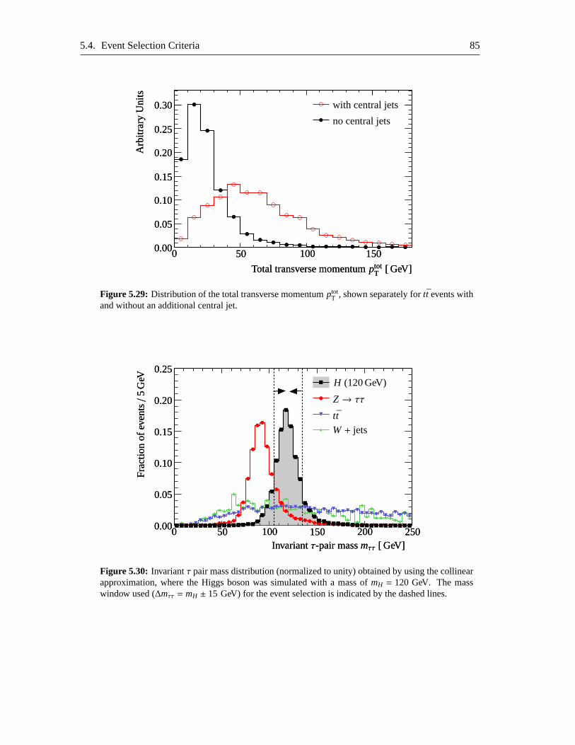
5.4. Event Selection Criteria 85
00 5050 100100 1501500.000.00
0.050.05
0.100.10
0.150.15
0.200.20
0.250.25
0.300.30
Arb
itrar
yU
nits
Arb
itrar
yU
nits
with central jets
no central jets
Total transverse momentumptotT [ GeV]Total transverse momentumptotT [ GeV]
Figure 5.29: Distribution of the total transverse momentumptotT , shown separately fortt events with
and without an additional central jet.
00 5050 100100 150150 200200 2502500.000.00
0.050.05
0.100.10
0.150.15
0.200.20
0.250.25
Z→ ττtt
W+ jets
Invariantτ-pair massmττ [ GeV]Invariantτ-pair massmττ [ GeV]
Fra
ctio
nof
even
ts/5
GeV
Fra
ctio
nof
even
ts/5
GeV H (120 GeV)
Figure 5.30: Invariantτ pair mass distribution (normalized to unity) obtained by using the collinearapproximation, where the Higgs boson was simulated with a mass ofmH = 120 GeV. The masswindow used (∆mττ = mH ± 15 GeV) for the event selection is indicated by the dashed lines.

86 Chapter 5. The Search for the Higgs Boson
Chapter 6
Optimization of the Signal Selection
The variables described in Section5.4can be used to separate signal and background events. Anoptimization of the cut values was performed in order to achieve a maximum signal significance.The cut optimization was done by scanning over the range of possible cut values for all variables.The set of cut values that results in a maximum of a predefined measure of the signal versusbackground separation is considered to be the optimal one.Several issues have to be addressed in order to obtain reliable cut values: the composition ofthe background processes, the preselection criteria, the definition of themeasure of the signal-to-background separation to be maximized, the set of variables used in the optimization and themethods for treating correlated variables. These aspects are discussedin the following.
6.1 Composition of the Background
The background consists of all processes that can be potentially misidentified as signal events.However, some of these processes could either not be simulated at all or with very low statisticsonly. For example, due to the low number of simulated events, including theW+ jets process in thebackground calculation would result in a high statistical uncertainty in the background prediction.Therefore, only the two most important background processes which have been simulated withsufficient statistics have been taken into account:Z→ ττ and tt. For theZ→ ττ background,the QCD as well as the electroweak production have been taken into account. The backgroundsamples have been combined by weighting them according to their cross-sections.
6.2 Preselection
In order to be able to calculate all discriminating variables, a few requirementsare necessary. Inaddition, several cuts have been fixed or the range of the possible cut values has been limitedbefore the optimization procedure for reasons discussed below. The preselection cuts are:
• Two visibleτ-decay products with opposite charge.
87
88 Chapter 6. Optimization of the Signal Selection
• The cut on the missing transverse energy is limited to the rangeEmissT > 40 GeV in the lep-
tonic channel and toEmissT > 30 GeV in the semileptonic channel. Hence, the strong suppres-
sion of all processes with no or only very little missing transverse energy (like Z→ ee, µµ)is ensured.
Due to the small amount of simulated data available for these processes, it hasnot beenpossible to reliably determine the rejection of these events by all the other cuts.To be con-servative, a minimum missing transverse energy was required. The lower minimum missingtransverse energy cut in the semileptonic analysis reflects the fact that in the hadronic decayof aτ lepton only one neutrino is involved leading to a lower missing energy in the event.
• The range for the lepton momentum fractionsχ1,2 is limited to the physical range fromzero to one. To allow for the collinear approximation, events with back-to-back leptons arerejected by limiting the∆φττ cut value to the range∆φττ < 2.9.
• In the semileptonic analysis,W+ jets is an important background while it is suppressed inthe leptonic analysis due to the low electron and muon misidentification rate. Also thenum-ber of simulatedW+ jets events was not sufficient to be included in the cut optimization.Therefore, a preselection cutmℓνT < 30 GeV is introduced to guarantee a strong suppressionof these events and the cut optimization is limited to the range belowmℓνT < 30 GeV.
• To account for the vector-boson fusion signature, two tagging jets in opposite hemispheresof the detector are required and both visibleτ-decay products have to be located within therapidity gap of these two jets.
• Since the central jet veto highly depends on the level of pile-up while data samples includingpile-up were not available with sufficient statistics for all the background processes, the cen-tral jet veto is not included in the optimization and has therefore been applied at preselectionlevel.
However, a possibility to take the impact of pile-up into account is to use inner detectorinformation to distinguish jets originating from separated vertices.
This approach has not been followed in the frame of this thesis but first studies [69] indicatethat this method allows for a central jet veto independent of the level of pile-up.
• Theb-jet veto is not included in the optimization as too littlett events with detailed detectorsimulation have been available. For the cut optimization, the fast detector simulation wasused for thett background. The fast simulation does not include ab-tagging algorithmproviding a continuously distributed variable for identification ofb jets (see Figure5.24),instead it assignsb jets tob quarks on a statistical basis. Therefore, there is no possibility tooptimize theb-jet veto and thus, it has been applied on the preselection level. Since thettbackground contribution is less important in the semileptonic than in the leptonic channel,theb-jet veto cut has only been applied in the leptonic analysis.
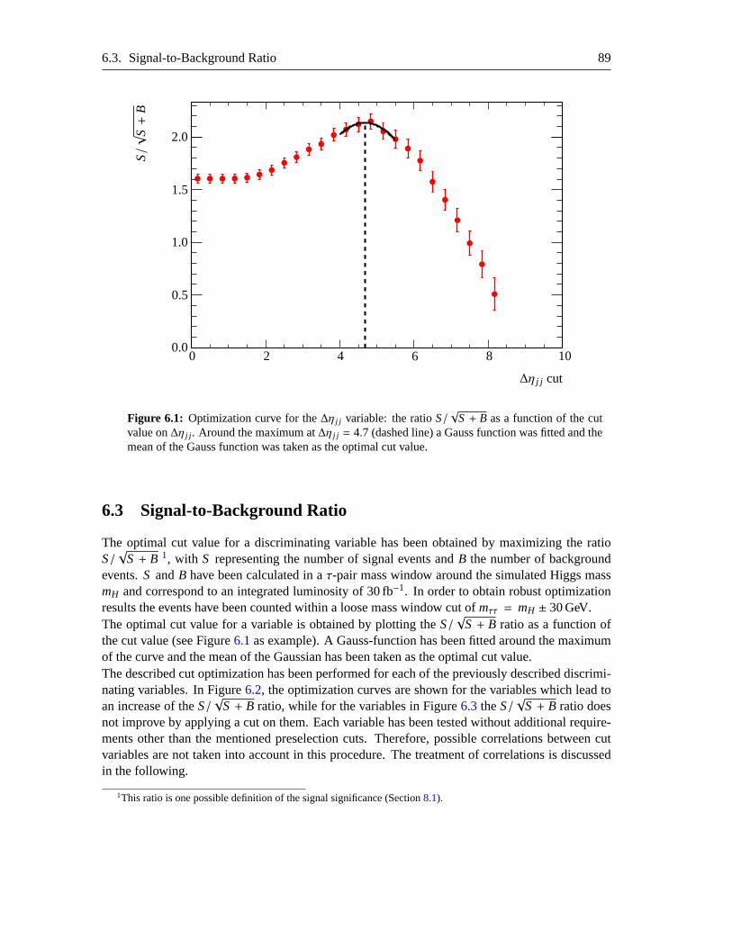
6.3. Signal-to-Background Ratio 89
0 2 4 6 8 100.0
0.5
1.0
1.5
2.0
miss
S/√
S+
B
∆η j j cut
Figure 6.1: Optimization curve for the∆η j j variable: the ratioS/√
S + B as a function of the cutvalue on∆η j j . Around the maximum at∆η j j = 4.7 (dashed line) a Gauss function was fitted and themean of the Gauss function was taken as the optimal cut value.
6.3 Signal-to-Background Ratio
The optimal cut value for a discriminating variable has been obtained by maximizing the ratioS/√
S + B 1, with S representing the number of signal events andB the number of backgroundevents.S andB have been calculated in aτ-pair mass window around the simulated Higgs massmH and correspond to an integrated luminosity of 30 fb−1. In order to obtain robust optimizationresults the events have been counted within a loose mass window cut ofmττ = mH ± 30 GeV.The optimal cut value for a variable is obtained by plotting theS/
√S + B ratio as a function of
the cut value (see Figure6.1as example). A Gauss-function has been fitted around the maximumof the curve and the mean of the Gaussian has been taken as the optimal cut value.The described cut optimization has been performed for each of the previously described discrimi-nating variables. In Figure6.2, the optimization curves are shown for the variables which lead toan increase of theS/
√S + B ratio, while for the variables in Figure6.3 theS/
√S + B ratio does
not improve by applying a cut on them. Each variable has been tested without additional require-ments other than the mentioned preselection cuts. Therefore, possible correlations between cutvariables are not taken into account in this procedure. The treatment of correlations is discussedin the following.
1This ratio is one possible definition of the signal significance (Section8.1).
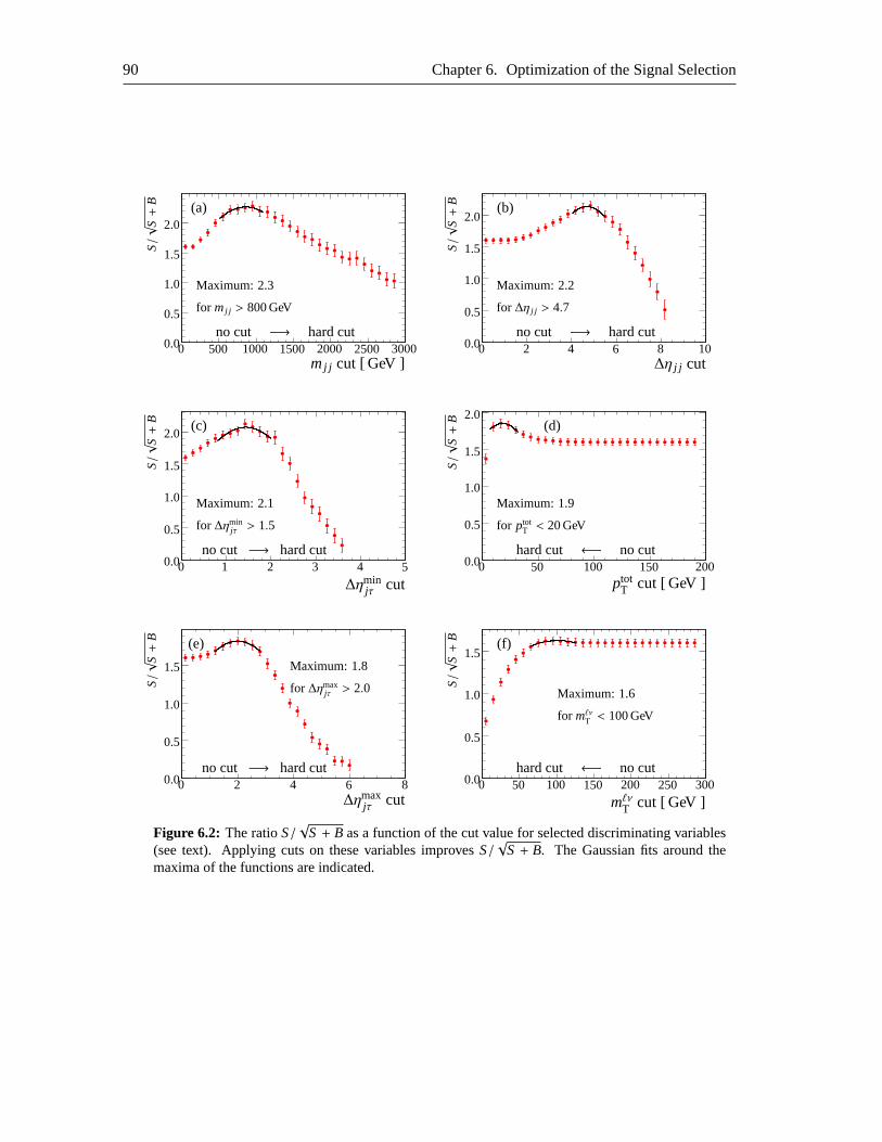
90 Chapter 6. Optimization of the Signal Selection
0 500 1000 1500 2000 2500 30000.0
0.5
1.0
1.5
2.0
Z
S/√
S+
B
mj j cut [ GeV ]
no cut −→ hard cut
Maximum: 2.3
for mj j > 800 GeV
(a)
0 2 4 6 8 100.0
0.5
1.0
1.5
2.0
S/√
S+
B
∆η j j cut
no cut −→ hard cut
Maximum: 2.2
for ∆η j j > 4.7
(b)
0 1 2 3 4 50.0
0.5
1.0
1.5
2.0
[
S/√
S+
B
∆ηminjτ cut
no cut −→ hard cut
Maximum: 2.1
for ∆ηminjτ > 1.5
(c)
0 50 100 150 2000.0
0.5
1.0
1.5
2.0
S/√
S+
B
ptotT cut [ GeV ]
hard cut ←− no cut
Maximum: 1.9
for ptotT < 20 GeV
(d)
0 2 4 6 80.0
0.5
1.0
1.5
S/√
S+
B
∆ηmaxjτ cut
no cut −→ hard cut
Maximum: 1.8
for ∆ηmaxjτ > 2.0
(e)
0 50 100 150 200 250 3000.0
0.5
1.0
1.5
S/√
S+
B
mℓνT cut [ GeV ]
hard cut ←− no cut
Maximum: 1.6
for mℓνT < 100 GeV
(f)
Figure 6.2: The ratioS/√
S + B as a function of the cut value for selected discriminating variables(see text). Applying cuts on these variables improvesS/
√S + B. The Gaussian fits around the
maxima of the functions are indicated.
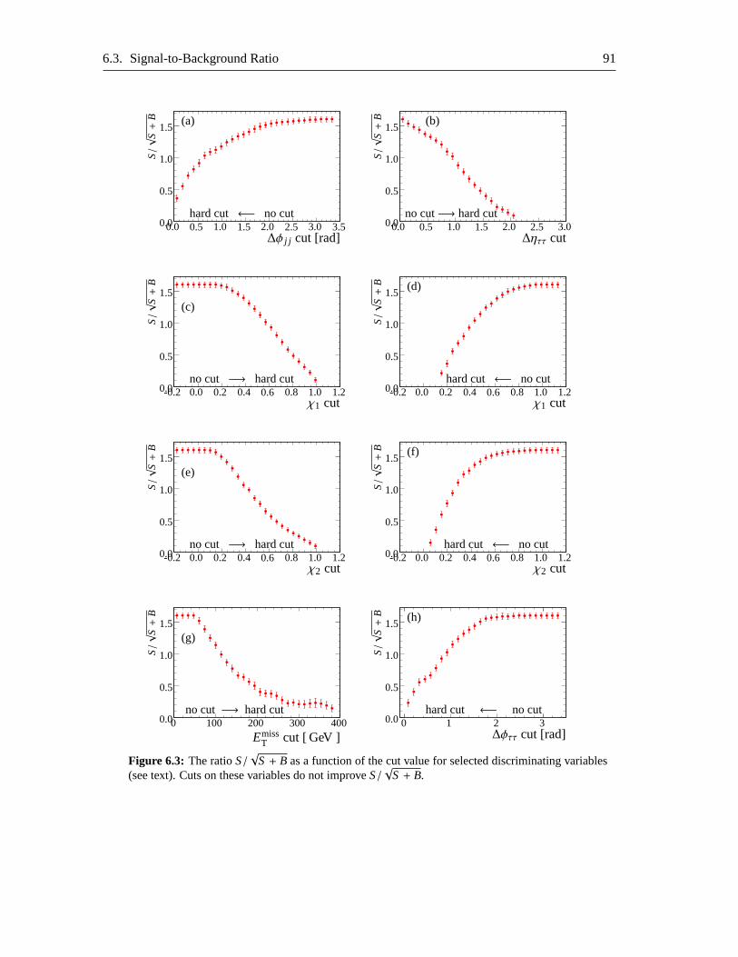
6.3. Signal-to-Background Ratio 91
0.00.0
0.5
0.5
1.0
1.0
1.5
1.5 2.0 2.5 3.0 3.5
→
S/√
S+
B
∆φ j j cut [rad]
hard cut ←− no cut
(a)
0.00.0
0.5
0.5
1.0
1.0
1.5
1.5 2.0 2.5 3.0
S/√
S+
B
∆ηττ cut
no cut−→ hard cut
(b)
-0.20.0 0.0 0.2 0.4
0.5
0.6 0.8
1.0
1.0 1.2
1.5
S/√
S+
B
χ1 cut
no cut −→ hard cut
(c)
-0.20.0 0.0 0.2 0.4
0.5
0.6 0.8
1.0
1.0 1.2
1.5
S/√
S+
B
χ1 cut
hard cut ←− no cut
(d)
-0.20.0 0.0 0.2 0.4
0.5
0.6 0.8
1.0
1.0 1.2
1.5
Fraction
S/√
S+
B
χ2 cut
no cut −→ hard cut
(e)
-0.20.0 0.0 0.2 0.4
0.5
0.6 0.8
1.0
1.0 1.2
1.5
S/√
S+
B
χ2 cut
hard cut ←− no cut
(f)
0 100 200 300 4000.0
0.5
1.0
1.5
S/√
S+
B
EmissT cut [ GeV ]
no cut −→ hard cut
(g)
0 1 2 30.0
0.5
1.0
1.5
S/√
S+
B
∆φττ cut [rad]
hard cut ←− no cut
(h)
Figure 6.3: The ratioS/√
S + B as a function of the cut value for selected discriminating variables(see text). Cuts on these variables do not improveS/
√S + B.

92 Chapter 6. Optimization of the Signal Selection
6.4 Treatment of Correlations
Two different approaches have been considered:
6.4.1 Parallel Cut Optimization
The most simple approach is to apply cuts only on the discriminating variables forwhich the cutimprovesS/
√S + B (the variables shown in Figure6.2: mj j , ∆η j j , ∆ηmin
jτ , ∆ηmaxjτ , ptot
T andmℓνT ).These variables are optimized in parallel, independently of each other. Thecut values obtaineddo not depend on the selection cuts on the other discriminating variables. Theresults of thisoptimization procedure are shown in Section6.6.
However, this method has two drawbacks:First, it does not take into account the effect of the other cuts on the signal-to-background ratio.Even if the shape of the distribution of a discriminating variable is not modified bya cut onanother variable, the numbers of signal and background events will change. Depending on thecut optimization criterion, this could result in a different optimal cut value. For example, if acut on another variable increased theS/B ratio such thatS > B, the ratioS/
√S + B approaches
S/√
S which has its maximum at the maximum number of signal eventsS. Thus, the cut on thisvariable would get very soft even if the ratioS/B would be increased by a harder cut. Therefore,the optimal cut value on a variable depends on the cuts on the other variables. If the cuts areoptimized independently, the cut values usually become too hard and the number of signal andbackground events is reduced too much compared to the global optimum. It maybe useful to omitcuts in order not to loose too many signal events, for example, using only thevariables with highseparation power. The result of this approach is also shown in Section6.6.
Second, not only the absolute number of events but also the shapes of distributions of discriminat-ing variables may change if a cut on a correlated variable is applied. Obviously, this will result ina different optimal cut value. As an example, Figure6.4shows the distribution of theη-separationof the two tagging jets∆η j j , before and after a cut on the invariant jet pair massmj j has beenapplied.
Since there is a correlation between the two variables, the shapes of the distributions depend oncuts which have been applied on them. Figure6.5shows the optimization of the cut on∆η j j withand without the prior cut on the invariant jet pair massmj j . The resulting optimal cut values of∆η j j > 4.7 (nomj j cut applied) and∆η j j > 3.8 (with mj j > 700 GeV applied) differ considerably.
Notice that with themj j > 700 GeV cut applied the optimal cut in∆η j j is lower than without thecut onmj j . Looking at the normalized∆η j j distributions (see Figure6.4) one would expect thecontrary. But, in this case, the effect of the reduced number of events exceeds the effect of theshape change of the∆η j j distribution.
For these reasons, the parallel cut optimization is quite unstable and the result depends on thepreselection cuts and the set of cuts optimized. This can be improved by iterating the optimizationprocedure, described in the following.
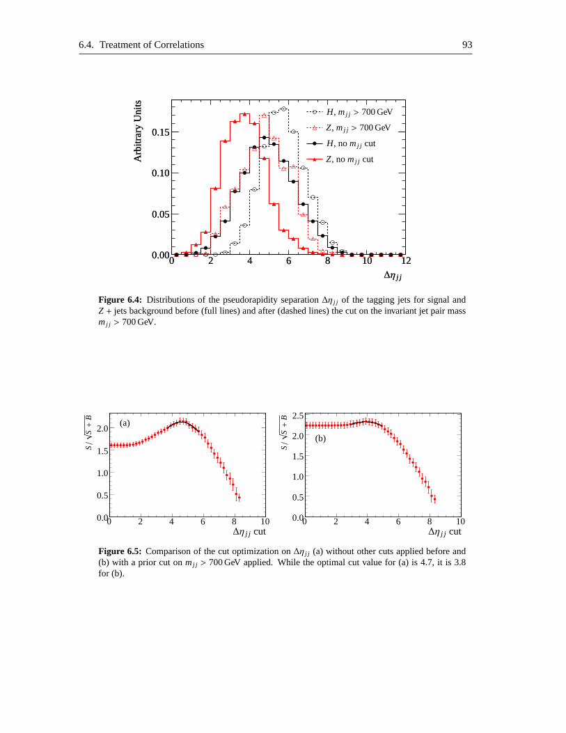
6.4. Treatment of Correlations 93
00 22 44 66 88 1010 12120.000.00
0.050.05
0.100.10
0.150.15A
rbitr
ary
Uni
tsA
rbitr
ary
Uni
ts
∆η j j∆η j j
H, nomj j cut
Z, nomj j cut
H, mj j > 700 GeV
Z, mj j > 700 GeV
Figure 6.4: Distributions of the pseudorapidity separation∆η j j of the tagging jets for signal andZ + jets background before (full lines) and after (dashed lines) the cut on the invariant jet pair massmj j > 700 GeV.
0 2 4 6 8 100.0
0.5
1.0
1.5
2.0
0.14
∆η j j cut
S/√
S+
B
(a)
0 2 4 6 8 100.0
0.5
1.0
1.5
2.0
2.5
∆η j j cut
S/√
S+
B
(b)
Figure 6.5: Comparison of the cut optimization on∆η j j (a) without other cuts applied before and(b) with a prior cut onmj j > 700 GeV applied. While the optimal cut value for (a) is 4.7, it is 3.8for (b).
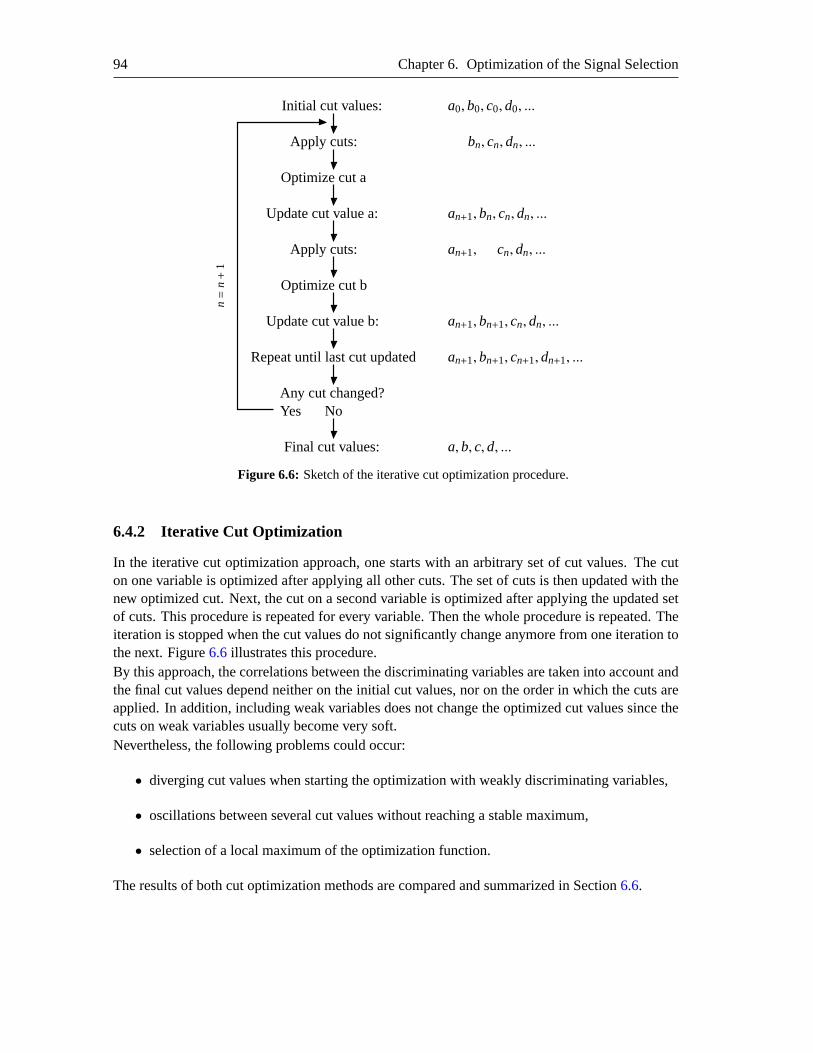
94 Chapter 6. Optimization of the Signal Selection
Initial cut values: a0,b0, c0,d0, ...
Apply cuts:
Apply cuts:
bn, cn,dn, ...
an+1, cn,dn, ...
Optimize cut a
Update cut value a: an+1,bn, cn,dn, ...
Optimize cut b
Update cut value b: an+1,bn+1, cn,dn, ...
Repeat until last cut updated an+1,bn+1, cn+1,dn+1, ...
Any cut changed?Yes No
Final cut values: a,b, c,d, ...
n=
n+
1
Figure 6.6: Sketch of the iterative cut optimization procedure.
6.4.2 Iterative Cut Optimization
In the iterative cut optimization approach, one starts with an arbitrary set ofcut values. The cuton one variable is optimized after applying all other cuts. The set of cuts is then updated with thenew optimized cut. Next, the cut on a second variable is optimized after applyingthe updated setof cuts. This procedure is repeated for every variable. Then the wholeprocedure is repeated. Theiteration is stopped when the cut values do not significantly change anymorefrom one iteration tothe next. Figure6.6 illustrates this procedure.By this approach, the correlations between the discriminating variables are taken into account andthe final cut values depend neither on the initial cut values, nor on the order in which the cuts areapplied. In addition, including weak variables does not change the optimizedcut values since thecuts on weak variables usually become very soft.Nevertheless, the following problems could occur:
• diverging cut values when starting the optimization with weakly discriminating variables,
• oscillations between several cut values without reaching a stable maximum,
• selection of a local maximum of the optimization function.
The results of both cut optimization methods are compared and summarized in Section 6.6.
6.5. Cut Efficiency Factorization for thett Background 95
6.5 Cut Efficiency Factorization for the t t Background
Due to the limited number of simulated events, even in case of thett dataset of the fast detec-tor simulation only very fewtt events survive all analysis selection criteria resulting in a largestatistical uncertainty on the prediction of thett background.In order to estimate thett contribution more reliably, the selection efficiency εmw of the masswindow cut has been determined with high statistics at an earlier stage of the analysis:
εmw =ni(mass window)
ni(whole mass range), (6.1)
whereni(mass window) is the number of events in a mass window around the Higgs peakandni(whole mass range) is the total number of events remaining after thei-th cut.Instead of applying the mass window cut at the end of the analysis the efficiencyεmw can be usedto calculate the number of events in the mass window,
nf (mass window)= εmw · nf (whole mass range), (6.2)
wherenf indicates the final number of events surviving all analysis cuts. With this masswin-dow factorization no events are rejected by the mass window cut and the statistical uncertainty isdecreased.It is assumed here that the efficiency factorεmw is independent of the subsequent cuts. However,the shape of the invariantττ-mass distribution (and thus the value ofεmw) doeschange with someof the selection cuts, for example by applying a cut on∆φττ as shown in Figure6.7. Nevertheless,up tomττ . 200 GeV themττ-shape is rather independent of the analysis cuts. Thus,εmw calcu-lated with respect to the number oftt events in a fixed subrange between 0 and 200 GeV,
εmw =ni(mass window)ni(0− 200 GeV)
(6.3)
can be assumed to be independent of the analysis cuts. Figure6.8shows the resulting value ofεmw
calculated in a mass window of 105− 135 GeV after applying one of the analysis cuts. Within thestatistical uncertainty, the mass window factorization for the mass windowmττ = 105− 135 GeVresults inεmw ∼ 20 %, independent of all other analysis cuts. The described factorization increasesthe tt statistics at the end of the analysis by a factor of 5 and thus allows for a more reliableprediction of thett background contribution.Since the mass window factorization is also applied during the cut optimization procedure (seeSection6), the influence of this factorization on the shape of the distributions of discriminatingvariables has been tested in addition. Figures6.9and6.10show the distributions of all discriminat-ing variables before and after the mass window factorization for a window of mττ = 90− 150 GeV.The factorization has only a minor influence on the∆φττ distribution and there is no significantimpact on the shape of all other distributions. Thus, it can be assumed that the mass windowfactorization does not introduce any large bias on the final analysis result.
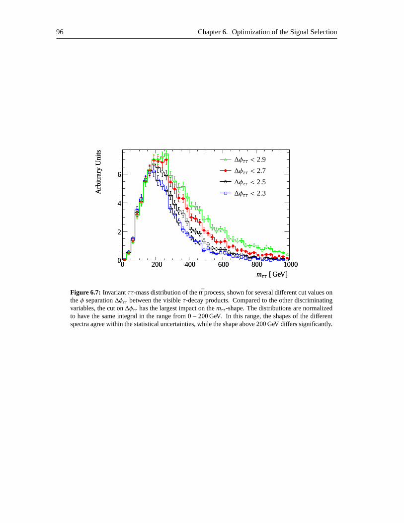
96 Chapter 6. Optimization of the Signal Selection
0000
22
44
66
200200 400400 600600 800800 10001000
Arb
itrar
yU
nits
Arb
itrar
yU
nits
mττ [ GeV]mττ [ GeV]
∆φττ < 2.3
∆φττ < 2.5
∆φττ < 2.7
∆φττ < 2.9
Figure 6.7: Invariantττ-mass distribution of thett process, shown for several different cut values ontheφ separation∆φττ between the visibleτ-decay products. Compared to the other discriminatingvariables, the cut on∆φττ has the largest impact on themττ-shape. The distributions are normalizedto have the same integral in the range from 0− 200 GeV. In this range, the shapes of the differentspectra agree within the statistical uncertainties, whilethe shape above 200 GeV differs significantly.
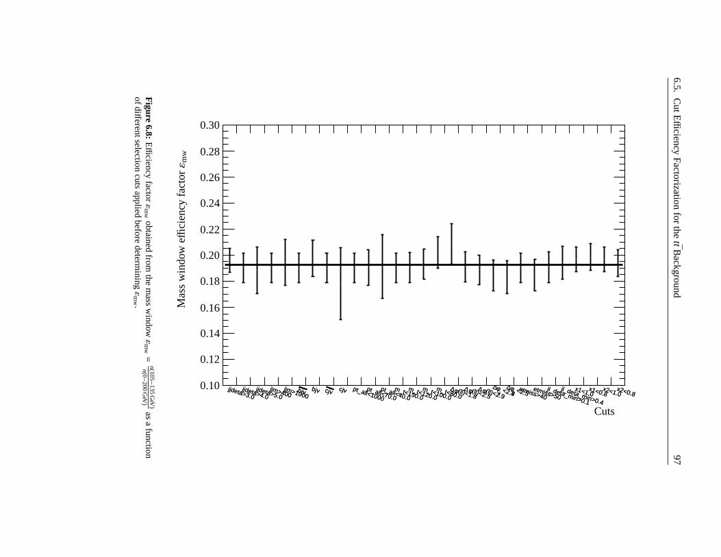
6.5.C
utEfficiency
Factorization
forthettB
ackground97
/ ndf χ 5.145 / 28
Prob 1
p0 0.0022± 0.1924
jjdeta>3.0jjdeta>4.0
jjdeta>5.0jjm>400
jjm>1000bjv bjv cjv cjv pt_all<1000
pt_all<70.0pt_all<40.0
m_t<150.0m_t<120.0
m_t<100.0m_t<80.0
(ll)<1.8φ∆ (ll)<2.5
φ∆ (ll)<2.9φ∆ <2.8jj
φ∆ <2.5jjφ∆ etmiss>40
etmiss>50jl_deta_min>0.1
jl_deta_min>0.4
x1<1.0x1<0.8
x2<1.0x2<0.8
jjdeta>3.0jjdeta>4.0
jjdeta>5.0jjm>400
jjm>1000bjv bjv cjv cjv pt_all<1000
pt_all<70.0pt_all<40.0
m_t<150.0m_t<120.0
m_t<100.0m_t<80.0
(ll)<1.8φ∆ (ll)<2.5
φ∆ (ll)<2.9φ∆ <2.8jj
φ∆ <2.5jjφ∆ etmiss>40
etmiss>50jl_deta_min>0.1
jl_deta_min>0.4
x1<1.0x1<0.8
x2<1.0x2<0.8
/ ndf χ 5.145 / 28
Prob 1
p0 0.0022± 0.1924
0.10
0.12
0.14
0.16
0.18
0.20
0.22
0.24
0.26
0.28
0.30
Mas
sw
indo
weffi
cien
cyfa
ctorε
mw
Cuts
Figure
6.8:Effi
ciencyfactorε
mw
obtainedfrom
them
assw
indowεmw=
n(105−135
GeV
)n(0−
200G
eV)
asa
functionofdiff
erentselectioncuts
appliedbefore
determiningε
mw .
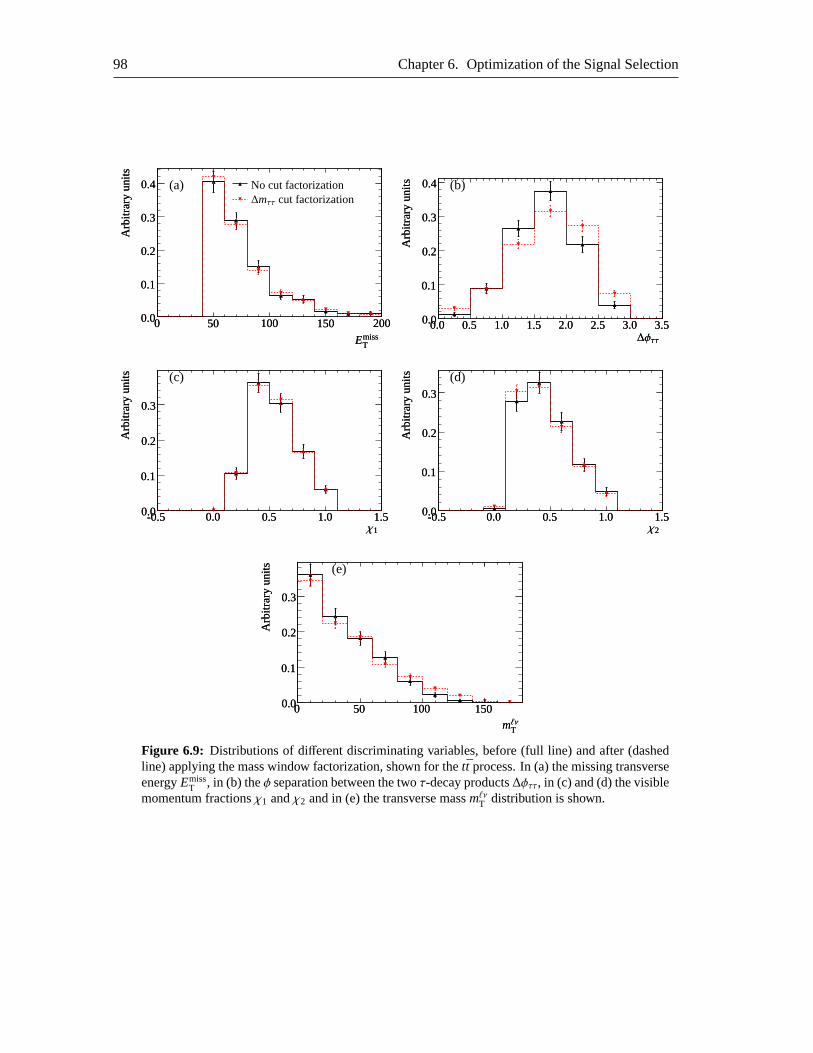
98 Chapter 6. Optimization of the Signal Selection
00 5050 100100 150150 2002000.00.0
0.10.1
0.20.2
0.30.3
0.40.4
jets
Arb
itrar
yun
itsA
rbitr
ary
units
No cut factorization∆mττ cut factorization
EmissTEmissT
(a)
0.00.00.00.0
0.10.1
0.20.2
0.30.3
0.40.4
0.50.5 1.01.0 1.51.5 2.02.0 2.52.5 3.03.0 3.53.5
Arb
itrar
yun
itsA
rbitr
ary
units
∆φττ∆φττ
(b)
-0.5-0.50.0 0.00.0 0.0
0.10.1
0.20.2
0.30.3
0.50.5 1.01.0 1.51.5
Ge
Arb
itrar
yun
itsA
rbitr
ary
units
χ1χ1
(c)
-0.5-0.50.0 0.00.0 0.0
0.10.1
0.20.2
0.30.3
0.50.5 1.01.0 1.51.5
Arb
itrar
yun
itsA
rbitr
ary
units
χ2χ2
(d)
00 5050 100100 1501500.00.0
0.10.1
0.20.2
0.30.3
Arb
itrar
yun
itsA
rbitr
ary
units
mℓνTmℓνT
(e)
Figure 6.9: Distributions of different discriminating variables, before (full line) and after (dashedline) applying the mass window factorization, shown for thett process. In (a) the missing transverseenergyEmiss
T , in (b) theφ separation between the twoτ-decay products∆φττ, in (c) and (d) the visiblemomentum fractionsχ1 andχ2 and in (e) the transverse massmℓνT distribution is shown.
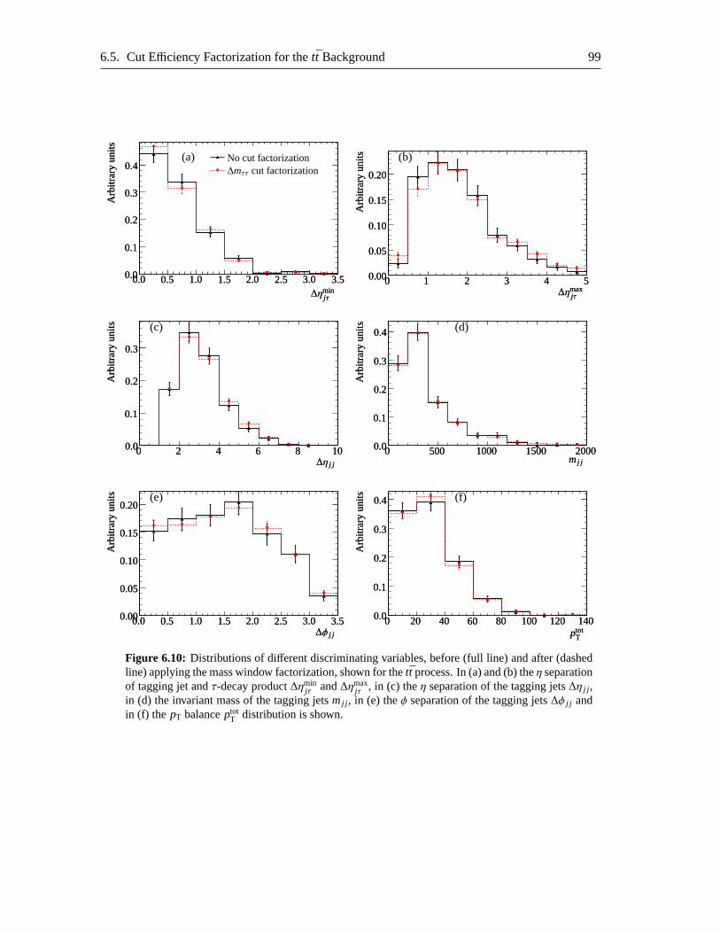
6.5. Cut Efficiency Factorization for thett Background 99
0.00.00.00.0
0.10.1
0.20.2
0.30.3
0.40.4
0.50.5 1.01.0 1.51.5 2.02.0 2.52.5 3.03.0 3.53.5
jets
Arb
itrar
yun
itsA
rbitr
ary
units
No cut factorization∆mττ cut factorization
∆ηminjτ∆ηminjτ
(a)
00 11 22 33 44 550.000.00
0.050.05
0.100.10
0.150.15
0.200.20
Arb
itrar
yun
itsA
rbitr
ary
units
∆ηmaxjτ∆ηmaxjτ
(b)
00 22 44 66 88 10100.00.0
0.10.1
0.20.2
0.30.3
Ge
Arb
itrar
yun
itsA
rbitr
ary
units
∆η j j∆η j j
(c)
00 500500 10001000 15001500 200020000.00.0
0.10.1
0.20.2
0.30.3
0.40.4
Arb
itrar
yun
itsA
rbitr
ary
units
mj jmj j
(d)
0.00.0 0.50.5 1.01.0 1.51.5 2.02.0 2.52.5 3.03.0 3.53.50.000.00
0.050.05
0.100.10
0.150.15
0.200.20
Ge
Arb
itrar
yun
itsA
rbitr
ary
units
∆φ j j∆φ j j
(e)
00 2020 4040 6060 8080 100100 120120 1401400.00.0
0.10.1
0.20.2
0.30.3
0.40.4
Arb
itrar
yun
itsA
rbitr
ary
units
ptotTptotT
(f)
Figure 6.10: Distributions of different discriminating variables, before (full line) and after (dashedline) applying the mass window factorization, shown for thett process. In (a) and (b) theη separationof tagging jet andτ-decay product∆ηmin
jτ and∆ηmaxjτ , in (c) theη separation of the tagging jets∆η j j ,
in (d) the invariant mass of the tagging jetsmj j , in (e) theφ separation of the tagging jets∆φ j j andin (f) the pT balanceptot
T distribution is shown.
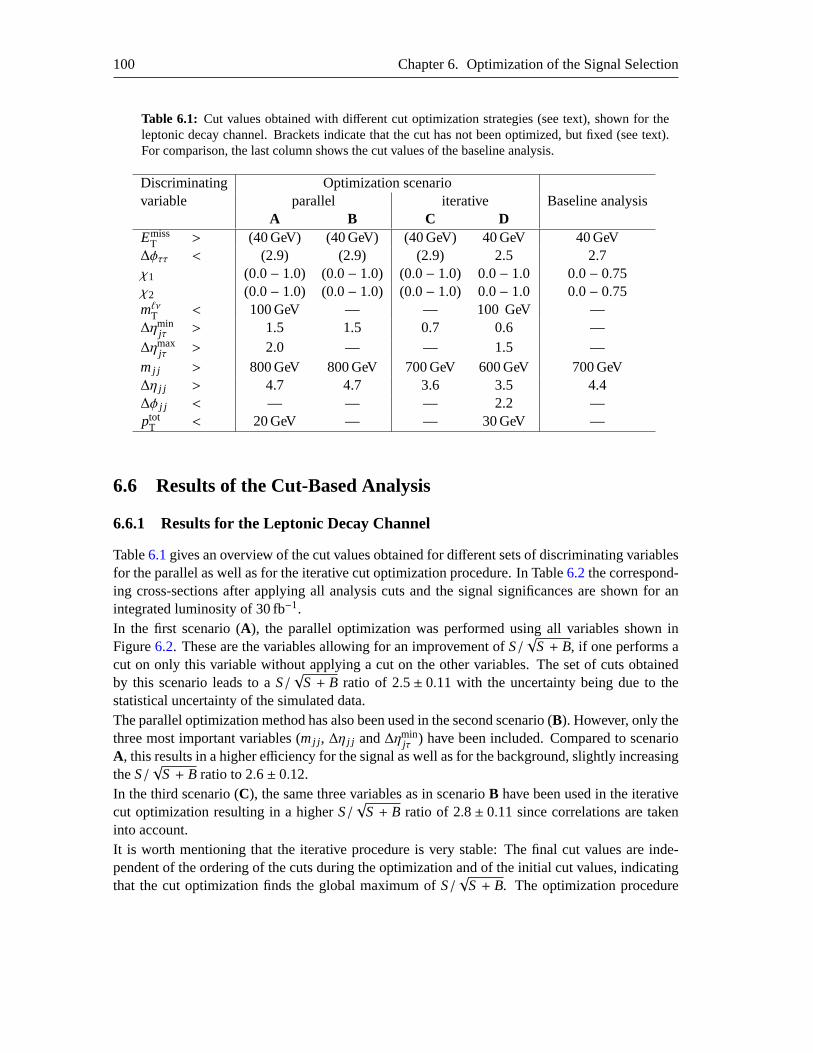
100 Chapter 6. Optimization of the Signal Selection
Table 6.1: Cut values obtained with different cut optimization strategies (see text), shown for theleptonic decay channel. Brackets indicate that the cut has not been optimized, but fixed (see text).For comparison, the last column shows the cut values of the baseline analysis.
Discriminating Optimization scenariovariable parallel iterative Baseline analysis
A B C DEmiss
T > (40 GeV) (40 GeV) (40 GeV) 40 GeV 40 GeV∆φττ < (2.9) (2.9) (2.9) 2.5 2.7χ1 (0.0− 1.0) (0.0− 1.0) (0.0− 1.0) 0.0− 1.0 0.0− 0.75χ2 (0.0− 1.0) (0.0− 1.0) (0.0− 1.0) 0.0− 1.0 0.0− 0.75mℓνT < 100 GeV — — 100 GeV —∆ηmin
jτ > 1.5 1.5 0.7 0.6 —∆ηmax
jτ > 2.0 — — 1.5 —mj j > 800 GeV 800 GeV 700 GeV 600 GeV 700 GeV∆η j j > 4.7 4.7 3.6 3.5 4.4∆φ j j < — — — 2.2 —ptot
T < 20 GeV — — 30 GeV —
6.6 Results of the Cut-Based Analysis
6.6.1 Results for the Leptonic Decay Channel
Table6.1gives an overview of the cut values obtained for different sets of discriminating variablesfor the parallel as well as for the iterative cut optimization procedure. In Table6.2the correspond-ing cross-sections after applying all analysis cuts and the signal significances are shown for anintegrated luminosity of 30 fb−1.In the first scenario (A), the parallel optimization was performed using all variables shown inFigure6.2. These are the variables allowing for an improvement ofS/
√S + B, if one performs a
cut on only this variable without applying a cut on the other variables. The set of cuts obtainedby this scenario leads to aS/
√S + B ratio of 2.5± 0.11 with the uncertainty being due to the
statistical uncertainty of the simulated data.The parallel optimization method has also been used in the second scenario (B). However, only thethree most important variables (mj j , ∆η j j and∆ηmin
jτ ) have been included. Compared to scenarioA, this results in a higher efficiency for the signal as well as for the background, slightly increasingtheS/
√S + B ratio to 2.6± 0.12.
In the third scenario (C), the same three variables as in scenarioB have been used in the iterativecut optimization resulting in a higherS/
√S + B ratio of 2.8± 0.11 since correlations are taken
into account.It is worth mentioning that the iterative procedure is very stable: The final cut values are inde-pendent of the ordering of the cuts during the optimization and of the initial cutvalues, indicatingthat the cut optimization finds the global maximum ofS/
√S + B. The optimization procedure
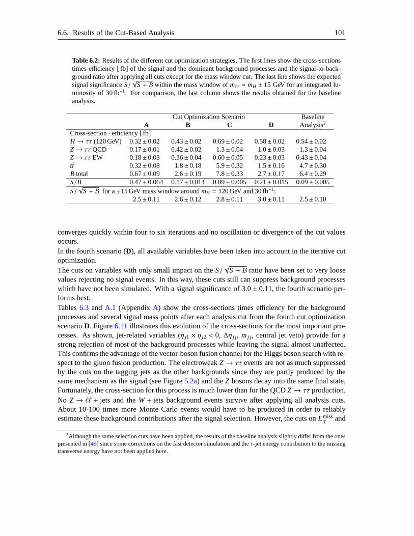
6.6. Results of the Cut-Based Analysis 101
Table 6.2: Results of the different cut optimization strategies. The first lines show the cross-sectionstimes efficiency [ fb] of the signal and the dominant background processes and the signal-to-back-ground ratio after applying all cuts except for the mass window cut. The last line shows the expectedsignal significanceS/
√S + B within the mass window ofmττ = mH ± 15 GeV for an integrated lu-
minosity of 30 fb−1. For comparison, the last column shows the results obtainedfor the baselineanalysis.
Cut Optimization Scenario BaselineA B C D Analysis2
Cross-section· efficiency [ fb]H → ττ (120 GeV) 0.32± 0.02 0.43± 0.02 0.69±0.02 0.58±0.02 0.54± 0.02Z→ ττ QCD 0.17± 0.01 0.42± 0.02 1.3±0.04 1.0±0.03 1.3± 0.04Z→ ττ EW 0.18± 0.03 0.36± 0.04 0.60±0.05 0.23±0.03 0.43± 0.04tt 0.32± 0.08 1.8± 0.18 5.9±0.32 1.5±0.16 4.7± 0.30B total 0.67± 0.09 2.6± 0.19 7.8±0.33 2.7±0.17 6.4± 0.29S/B 0.47± 0.064 0.17± 0.014 0.09±0.005 0.21±0.015 0.09± 0.005S/√
S + B for a±15 GeV mass window aroundmH = 120 GeV and 30 fb−1:2.5± 0.11 2.6± 0.12 2.8±0.11 3.0±0.11 2.5± 0.10
converges quickly within four to six iterations and no oscillation or divergence of the cut valuesoccurs.In the fourth scenario (D), all available variables have been taken into account in the iterative cutoptimization.The cuts on variables with only small impact on theS/
√S + B ratio have been set to very loose
values rejecting no signal events. In this way, these cuts still can suppress background processeswhich have not been simulated. With a signal significance of 3.0± 0.11, the fourth scenario per-forms best.Tables6.3 and A.1 (Appendix A) show the cross-sections times efficiency for the backgroundprocesses and several signal mass points after each analysis cut from the fourth cut optimizationscenarioD. Figure6.11illustrates this evolution of the cross-sections for the most important pro-cesses. As shown, jet-related variables (η j1 × η j2 < 0, ∆η j j , mj j , central jet veto) provide for astrong rejection of most of the background processes while leaving the signal almost unaffected.This confirms the advantage of the vector-boson fusion channel for theHiggs boson search with re-spect to the gluon fusion production. The electroweakZ→ ττ events are not as much suppressedby the cuts on the tagging jets as the other backgrounds since they are partlyproduced by thesame mechanism as the signal (see Figure5.2a) and theZ bosons decay into the same final state.Fortunately, the cross-section for this process is much lower than for the QCD Z→ ττ production.No Z→ ℓℓ + jets and theW+ jets background events survive after applying all analysis cuts.About 10-100 times more Monte Carlo events would have to be produced in order to reliablyestimate these background contributions after the signal selection. However, the cuts onEmiss
T and
2Although the same selection cuts have been applied, the results of the baseline analysis slightly differ from the onespresented in [49] since some corrections on the fast detector simulation and theτ-jet energy contribution to the missingtransverse energy have not been applied here.
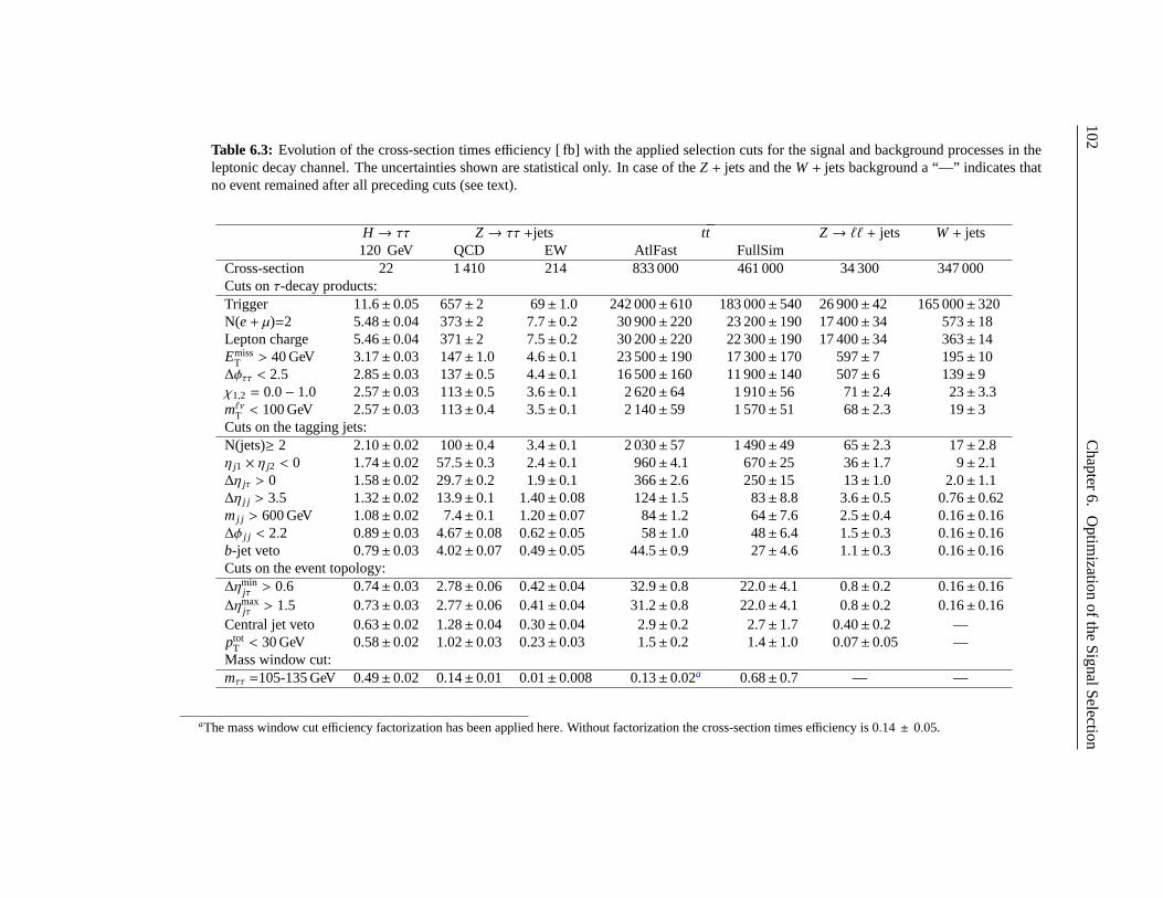
102C
hapter6.
Optim
izationofthe
SignalS
election
Table 6.3: Evolution of the cross-section times efficiency [ fb] with the applied selection cuts for the signal and background processes in theleptonic decay channel. The uncertainties shown are statistical only. In case of theZ + jets and theW+ jets background a “—” indicates thatno event remained after all preceding cuts (see text).
H → ττ Z→ ττ +jets tt Z→ ℓℓ + jets W+ jets120 GeV QCD EW AtlFast FullSim
Cross-section 22 1 410 214 833 000 461 000 34 300 347 000Cuts onτ-decay products:Trigger 11.6±0.05 657± 2 69± 1.0 242 000±610 183 000±540 26 900± 42 165 000±320N(e+ µ)=2 5.48±0.04 373± 2 7.7± 0.2 30 900±220 23 200±190 17 400± 34 573±18Lepton charge 5.46±0.04 371± 2 7.5± 0.2 30 200±220 22 300±190 17 400± 34 363±14Emiss
T > 40 GeV 3.17±0.03 147± 1.0 4.6± 0.1 23 500±190 17 300±170 597± 7 195±10∆φττ < 2.5 2.85±0.03 137± 0.5 4.4± 0.1 16 500±160 11 900±140 507± 6 139±9χ1,2 = 0.0− 1.0 2.57±0.03 113± 0.5 3.6± 0.1 2 620±64 1 910±56 71± 2.4 23±3.3mℓνT < 100 GeV 2.57±0.03 113± 0.4 3.5± 0.1 2 140±59 1 570±51 68± 2.3 19±3Cuts on the tagging jets:N(jets)≥ 2 2.10±0.02 100± 0.4 3.4± 0.1 2 030±57 1 490±49 65± 2.3 17±2.8η j1 × η j2 < 0 1.74±0.02 57.5± 0.3 2.4± 0.1 960±4.1 670±25 36± 1.7 9±2.1∆η jτ > 0 1.58±0.02 29.7± 0.2 1.9± 0.1 366±2.6 250±15 13± 1.0 2.0±1.1∆η j j > 3.5 1.32±0.02 13.9± 0.1 1.40± 0.08 124±1.5 83±8.8 3.6± 0.5 0.76±0.62mj j > 600 GeV 1.08±0.02 7.4± 0.1 1.20± 0.07 84±1.2 64±7.6 2.5± 0.4 0.16±0.16∆φ j j < 2.2 0.89±0.03 4.67± 0.08 0.62± 0.05 58±1.0 48±6.4 1.5± 0.3 0.16±0.16b-jet veto 0.79±0.03 4.02± 0.07 0.49± 0.05 44.5±0.9 27±4.6 1.1± 0.3 0.16±0.16Cuts on the event topology:∆ηmin
jτ > 0.6 0.74±0.03 2.78± 0.06 0.42± 0.04 32.9±0.8 22.0±4.1 0.8± 0.2 0.16±0.16∆ηmax
jτ > 1.5 0.73±0.03 2.77± 0.06 0.41± 0.04 31.2±0.8 22.0±4.1 0.8± 0.2 0.16±0.16Central jet veto 0.63±0.02 1.28± 0.04 0.30± 0.04 2.9±0.2 2.7±1.7 0.40± 0.2 —ptot
T < 30 GeV 0.58±0.02 1.02± 0.03 0.23± 0.03 1.5±0.2 1.4±1.0 0.07± 0.05 —Mass window cut:mττ =105-135 GeV 0.49±0.02 0.14± 0.01 0.01± 0.008 0.13±0.02a 0.68±0.7 — —
aThe mass window cut efficiency factorization has been applied here. Without factorization the cross-section times efficiency is 0.14 ± 0.05.
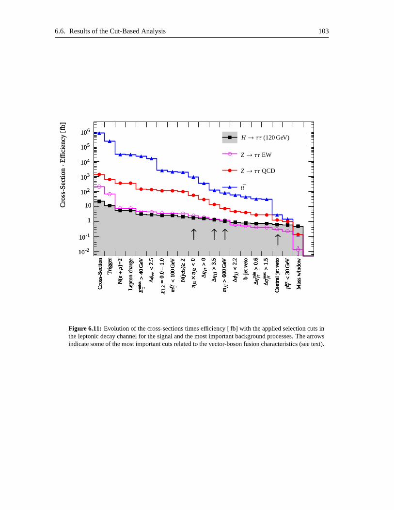
6.6. Results of the Cut-Based Analysis 103
11
10
10
10
10
10
10
10
10
10
10
10
10
10
10
10
10
jets
-1-1
-2-2
22
33
44
55
66
Cro
ss-S
ectio
n·Effi
cien
cy[fb
]C
ross
-Sec
tion·Effi
cien
cy[fb
]
H → ττ (120 GeV)
Z→ ττ EW
Z→ ττ QCD
tt
Cro
ss-S
ectio
nC
ross
-Sec
tion
Cro
ss-S
ectio
nC
ross
-Sec
tion
Trig
ger
Trig
ger
Trig
ger
Trig
ger
N(e+µ)=
2N
(e+µ)=
2N
(e+µ)=
2N
(e+µ)=
2
Lept
onch
arge
Lept
onch
arge
Lept
onch
arge
Lept
onch
arge
Em
iss
T>
40G
eVE
mis
sT>
40G
eVE
mis
sT>
40G
eVE
mis
sT>
40G
eV
∆φττ<
2.5
∆φττ<
2.5
∆φττ<
2.5
∆φττ<
2.5
χ1,
2=
0.0−
1.0
χ1,
2=
0.0−
1.0
χ1,
2=
0.0−
1.0
χ1,
2=
0.0−
1.0
mℓν T<
100
GeV
mℓν T<
100
GeV
mℓν T<
100
GeV
mℓν T<
100
GeV
N(je
ts)≥
2N
(jets
)≥2
N(je
ts)≥
2N
(jets
)≥2
ηj1×η
j2<
0η
j1×η
j2<
0η
j1×η
j2<
0η
j1×η
j2<
0
∆η
jτ>
0∆η
jτ>
0∆η
jτ>
0∆η
jτ>
0
∆η
jj>
3.5
∆η
jj>
3.5
∆η
jj>
3.5
∆η
jj>
3.5
mjj>
600
GeV
mjj>
600
GeV
mjj>
600
GeV
mjj>
600
GeV
∆φ
jj<
2.2
∆φ
jj<
2.2
∆φ
jj<
2.2
∆φ
jj<
2.2
b-je
tvet
ob-
jetv
eto
b-je
tvet
ob-
jetv
eto
∆η
min
jτ>
0.6
∆η
min
jτ>
0.6
∆η
min
jτ>
0.6
∆η
min
jτ>
0.6
∆η
max
jτ>
1.5
∆η
max
jτ>
1.5
∆η
max
jτ>
1.5
∆η
max
jτ>
1.5
Cen
tral
jetv
eto
Cen
tral
jetv
eto
Cen
tral
jetv
eto
Cen
tral
jetv
eto
ptot
T<
30G
eVpto
tT<
30G
eVpto
tT<
30G
eVpto
tT<
30G
eV
Mas
sw
indo
wM
ass
win
dow
Mas
sw
indo
wM
ass
win
dow
↑ ↑ ↑ ↑
Figure 6.11: Evolution of the cross-sections times efficiency [ fb] with the applied selection cuts inthe leptonic decay channel for the signal and the most important background processes. The arrowsindicate some of the most important cuts related to the vector-boson fusion characteristics (see text).
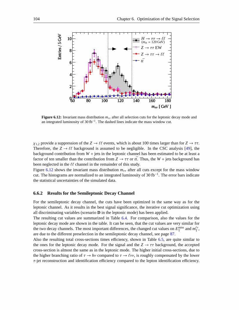
104 Chapter 6. Optimization of the Signal Selection
000
222
444
666
888
101010
606060 808080 100100100 120120120 140140140 160160160 180180180
Z→ ττ EW
Z→ ττ→ ℓℓtt
mττ [ GeV ]mττ [ GeV ]mττ [ GeV ]
Ent
ries/
5G
eVE
ntrie
s/5
GeV
Ent
ries/
5G
eV H → ττ→ ℓℓ(mH = 120 GeV)
Figure 6.12: Invariant mass distributionmττ after all selection cuts for the leptonic decay mode andan integrated luminosity of 30 fb−1. The dashed lines indicate the mass window cut.
χ1,2 provide a suppression of theZ→ ℓℓ events, which is about 100 times larger than forZ→ ττ.Therefore, theZ→ ℓℓ background is assumed to be negligible. In the CSC analysis [49], thebackground contribution fromW+ jets in the leptonic channel has been estimated to be at least afactor of ten smaller than the contribution fromZ→ ττ or tt. Thus, theW+ jets background hasbeen neglected in theℓℓ channel in the remainder of this study.Figure6.12shows the invariant mass distributionmττ after all cuts except for the mass windowcut. The histograms are normalized to an integrated luminosity of 30 fb−1. The error bars indicatethe statistical uncertainties of the simulated data.
6.6.2 Results for the Semileptonic Decay Channel
For the semileptonic decay channel, the cuts have been optimized in the same wayas for theleptonic channel. As it results in the best signal significance, the iterative cut optimization usingall discriminating variables (scenarioD in the leptonic mode) has been applied.The resulting cut values are summarized in Table6.4. For comparison, also the values for theleptonic decay mode are shown in the table. It can be seen, that the cut values are very similar forthe two decay channels. The most important differences, the changed cut values onEmiss
T andmℓνT ,are due to the different preselection in the semileptonic decay channel, see page87.Also the resulting total cross-sections times efficiency, shown in Table6.5, are quite similar tothe ones for the leptonic decay mode. For the signal and theZ→ ττ background, the acceptedcross-section is almost the same as in the leptonic mode. The higher initial cross-sections, due tothe higher branching ratio ofτ→ hν compared toτ→ ℓνν, is roughly compensated by the lowerτ-jet reconstruction and identification efficiency compared to the lepton identification efficiency.

6.6. Results of the Cut-Based Analysis 105
Table 6.4: Cut values obtained with the iterative optimization methodfor the semileptonic decaychannel. For comparison, the cut values for the leptonic decay channel (see Table6.1, scenarioD)and the cut values applied in the baseline analysis are shown.
Optimized cuts Baseline analysisDecay channel ℓℓ ℓh ℓhEmiss
T > 40 GeV 30 GeV 40 GeV∆φττ < 2.5 2.5 2.7χℓ 0.0− 1.0 0.0− 1.0 0.0− 0.75χh — 0.0− 1.0 0.0− 1.0mℓνT < 100 GeV 30 GeV 30 GeV∆ηmin
jτ > 0.6 0.8 —∆ηmax
jτ > 1.5 1.5 —mj j > 600 GeV 600 GeV 700 GeV∆η j j > 3.5 3.6 4.4∆φ j j < 2.2 2.7 —ptot
T < 30 GeV 40 GeV —
Table 6.5: Results for the semileptonic channel: Cross-sections times efficiency [ fb] of the signaland the dominant background processes, signal-to-background ratio after applying all cuts exceptfor the mass window cut and expected signal significanceS/
√S + B within the mass window of
mττ = mH ± 15 GeV for an integrated luminosity of 30 fb−1. For comparison, the results for theleptonic decay channel (see Table6.2, scenarioD) and for the baseline analysis are shown.
Optimized cuts Baseline analysisDecay channel ℓℓ ℓh ℓhCross-section· efficiency [ fb]H → ττ (120 GeV) 0.58±0.02 0.67±0.04 0.67±0.04Z→ ττ QCD 1.0±0.03 1.0±0.09 1.2±0.10Z→ ττ EW 0.23±0.03 0.38±0.04 0.46±0.05tt 1.5±0.16 0.14±0.05 0.28±0.07B total 2.7±0.17 1.5±0.11 1.6±0.10S/B 0.21±0.02 0.44±0.04 0.35±0.03S/√
S + B for a±15 GeV mass window aroundmH = 120 GeV and 30 fb−1:
3.0±0.11 3.7±0.15 3.6±0.15
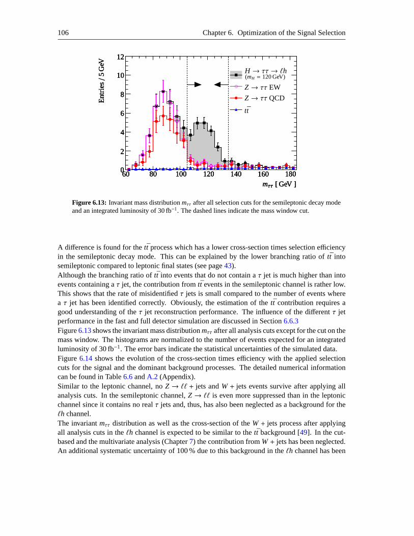
106 Chapter 6. Optimization of the Signal Selection
000
222
444
666
888
101010
121212
606060 808080 100100100 120120120 140140140 160160160 180180180
Z→ ττ QCD
Z→ ττ EW
tt
mττ [ GeV ]mττ [ GeV ]mττ [ GeV ]
Ent
ries/
5G
eVE
ntrie
s/5
GeV
Ent
ries/
5G
eV
H → ττ→ ℓh(mH = 120 GeV)
Figure 6.13: Invariant mass distributionmττ after all selection cuts for the semileptonic decay modeand an integrated luminosity of 30 fb−1. The dashed lines indicate the mass window cut.
A difference is found for thett process which has a lower cross-section times selection efficiencyin the semileptonic decay mode. This can be explained by the lower branching ratio of tt intosemileptonic compared to leptonic final states (see page43).Although the branching ratio oftt into events that do not contain aτ jet is much higher than intoevents containing aτ jet, the contribution fromtt events in the semileptonic channel is rather low.This shows that the rate of misidentifiedτ jets is small compared to the number of events wherea τ jet has been identified correctly. Obviously, the estimation of thett contribution requires agood understanding of theτ jet reconstruction performance. The influence of the differentτ jetperformance in the fast and full detector simulation are discussed in Section6.6.3Figure6.13shows the invariant mass distributionmττ after all analysis cuts except for the cut on themass window. The histograms are normalized to the number of events expectedfor an integratedluminosity of 30 fb−1. The error bars indicate the statistical uncertainties of the simulated data.Figure6.14 shows the evolution of the cross-section times efficiency with the applied selectioncuts for the signal and the dominant background processes. The detailed numerical informationcan be found in Table6.6andA.2 (Appendix).Similar to the leptonic channel, noZ→ ℓℓ + jets andW+ jets events survive after applying allanalysis cuts. In the semileptonic channel,Z→ ℓℓ is even more suppressed than in the leptonicchannel since it contains no realτ jets and, thus, has also been neglected as a background for theℓh channel.The invariantmττ distribution as well as the cross-section of theW+ jets process after applyingall analysis cuts in theℓh channel is expected to be similar to thett background [49]. In the cut-based and the multivariate analysis (Chapter7) the contribution fromW+ jets has been neglected.An additional systematic uncertainty of 100 % due to this background in theℓh channel has been
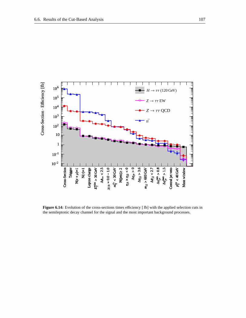
6.6. Results of the Cut-Based Analysis 107
11
10
10
10
10
10
10
10
10
10
10
10
10
10
10
10
10
Z→ ττ QCD
+
-1-1
-2-2
22
33
44
55
66
Cro
ss-S
ectio
n·Effi
cien
cy[fb
]C
ross
-Sec
tion·Effi
cien
cy[fb
]
H → ττ (120 GeV)
Z→ ττ EW
tt
Cro
ss-S
ectio
nC
ross
-Sec
tion
Cro
ss-S
ectio
nC
ross
-Sec
tion
Trig
ger
Trig
ger
Trig
ger
Trig
ger
N(e+µ)=
1N
(e+µ)=
1N
(e+µ)=
1N
(e+µ)=
1
N(τ
)=1
N(τ
)=1
N(τ
)=1
N(τ
)=1
Lept
onch
arge
Lept
onch
arge
Lept
onch
arge
Lept
onch
arge
Em
iss
T>
30G
eVE
mis
sT>
30G
eVE
mis
sT>
30G
eVE
mis
sT>
30G
eV
∆φττ<
2.5
∆φττ<
2.5
∆φττ<
2.5
∆φττ<
2.5
χℓ,
h=
0.0−
1.0
χℓ,
h=
0.0−
1.0
χℓ,
h=
0.0−
1.0
χℓ,
h=
0.0−
1.0
mℓν T<
30G
eVmℓν T<
30G
eVmℓν T<
30G
eVmℓν T<
30G
eV
N(je
ts)≥
2N
(jets
)≥2
N(je
ts)≥
2N
(jets
)≥2
ηj1×η
j2<
0η
j1×η
j2<
0η
j1×η
j2<
0η
j1×η
j2<
0
∆η
jτ>
0∆η
jτ>
0∆η
jτ>
0∆η
jτ>
0
∆η
jj>
3.6
∆η
jj>
3.6
∆η
jj>
3.6
∆η
jj>
3.6
mjj>
600
GeV
mjj>
600
GeV
mjj>
600
GeV
mjj>
600
GeV
∆φ
jj<
2.7
∆φ
jj<
2.7
∆φ
jj<
2.7
∆φ
jj<
2.7
∆η
min
jτ>
0.8
∆η
min
jτ>
0.8
∆η
min
jτ>
0.8
∆η
min
jτ>
0.8
∆η
max
jτ>
1.5
∆η
max
jτ>
1.5
∆η
max
jτ>
1.5
∆η
max
jτ>
1.5
Cen
tral
jetv
eto
Cen
tral
jetv
eto
Cen
tral
jetv
eto
Cen
tral
jetv
eto
ptot
T<
40G
eVpto
tT<
40G
eVpto
tT<
40G
eVpto
tT<
40G
eV
Mas
sw
indo
wM
ass
win
dow
Mas
sw
indo
wM
ass
win
dow
Figure 6.14: Evolution of the cross-sections times efficiency [ fb] with the applied selection cuts inthe semileptonic decay channel for the signal and the most important background processes.
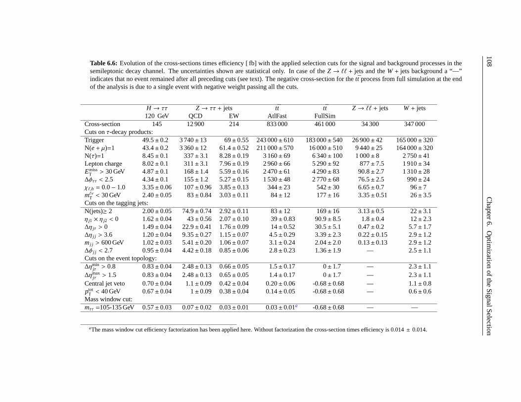
108C
hapter6.
Optim
izationofthe
SignalS
election
Table 6.6: Evolution of the cross-sections times efficiency [ fb] with the applied selection cuts for the signal and background processes in thesemileptonic decay channel. The uncertainties shown are statistical only. In case of theZ→ ℓℓ + jets and theW+ jets background a “—”indicates that no event remained after all preceding cuts (see text). The negative cross-section for thett process from full simulation at the endof the analysis is due to a single event with negative weight passing all the cuts.
H → ττ Z→ ττ + jets tt tt Z→ ℓℓ + jets W+ jets120 GeV QCD EW AtlFast FullSim
Cross-section 145 12 900 214 833 000 461 000 34 300 347 000Cuts onτ-decay products:Trigger 49.5± 0.2 3 740± 13 69± 0.55 243 000± 610 183 000± 540 26 900±42 165 000±320N(e+ µ)=1 43.4± 0.2 3 360± 12 61.4± 0.52 211 000± 570 16 000± 510 9 440±25 164 000±320N(τ)=1 8.45± 0.1 337± 3.1 8.28± 0.19 3 160± 69 6 340± 100 1 000±8 2 750±41Lepton charge 8.02± 0.1 311± 3.1 7.96± 0.19 2 960± 66 5 290± 92 877±7.5 1 910±34Emiss
T > 30 GeV 4.87± 0.1 168± 1.4 5.59± 0.16 2 470± 61 4 290± 83 90.8±2.7 1 310±28∆φττ < 2.5 4.34± 0.1 155± 1.2 5.27± 0.15 1 530± 48 2 770± 68 76.5±2.5 990±24χℓ,h = 0.0− 1.0 3.35± 0.06 107± 0.96 3.85± 0.13 344± 23 542± 30 6.65±0.7 96±7mℓνT < 30 GeV 2.40± 0.05 83± 0.84 3.03± 0.11 84± 12 177± 16 3.35±0.51 26±3.5Cuts on the tagging jets:N(jets)≥ 2 2.00± 0.05 74.9± 0.74 2.92± 0.11 83± 12 169± 16 3.13±0.5 22±3.1η j1 × η j2 < 0 1.62± 0.04 43± 0.56 2.07± 0.10 39± 0.83 90.9± 8.5 1.8±0.4 12±2.3∆η jτ > 0 1.49± 0.04 22.9± 0.41 1.76± 0.09 14± 0.52 30.5± 5.1 0.47±0.2 5.7±1.7∆η j j > 3.6 1.20± 0.04 9.35± 0.27 1.15± 0.07 4.5± 0.29 3.39± 2.3 0.22±0.15 2.9±1.2mj j > 600 GeV 1.02± 0.03 5.41± 0.20 1.06± 0.07 3.1± 0.24 2.04± 2.0 0.13±0.13 2.9±1.2∆φ j j < 2.7 0.95± 0.04 4.42± 0.18 0.85± 0.06 2.8± 0.23 1.36± 1.9 — 2.5±1.1Cuts on the event topology:∆ηmin
jτ > 0.8 0.83± 0.04 2.48± 0.13 0.66± 0.05 1.5± 0.17 0± 1.7 — 2.3±1.1∆ηmax
jτ > 1.5 0.83± 0.04 2.48± 0.13 0.65± 0.05 1.4± 0.17 0± 1.7 — 2.3±1.1Central jet veto 0.70± 0.04 1.1± 0.09 0.42± 0.04 0.20± 0.06 -0.68± 0.68 — 1.1±0.8ptot
T < 40 GeV 0.67± 0.04 1± 0.09 0.38± 0.04 0.14± 0.05 -0.68± 0.68 — 0.6±0.6Mass window cut:mττ =105-135 GeV 0.57± 0.03 0.07± 0.02 0.03± 0.01 0.03± 0.01a -0.68± 0.68 — —
aThe mass window cut efficiency factorization has been applied here. Without factorization the cross-section times efficiency is 0.014 ± 0.014.

6.6. Results of the Cut-Based Analysis 109
introduced when calculating the signal significances with background estimation based on MonteCarlo in Section8.2.4, assuming that the shape of themττ distribution is the same for theW+ jetsandtt contribution.
6.6.3 Comparison of Detailed and Fast Simulation for thet t Background
Due to the high cross-section fortt production, it is not possible to simulate a sufficient number oftt events using the full detector simulation. Therefore, the data sample simulated with ATLFASThas been used for the described analysis.In Section5.2 the detector performance determined from the full and the ATLFAST simulationisdescribed. Here, the impact of using ATLFAST on the prediction of thett background in the pre-sented analysis is discussed. The most relevant differences between the full and the fast simulationare:
• Electron and Muon TriggerSince no trigger simulation is performed in the fast simulation, a reconstructed lepton withminimum pT is required to represent the trigger selection in the analysis of events fromthefast simulation. An event is considered to be accepted by the trigger if an electron withpe
T ≥ 25 GeV and/or a muon withpµT ≥ 20 GeV is present. Noτ-jet trigger was used in theanalysis (see Section5.2.1).
The last two columns of Table6.7 show the efficiency of the trigger requirementsafterrequiring two reconstructedτ-decay products with opposite charge. In the leptonic decaychannel, about 10 % of thett events are rejected by the trigger in the detailed simulation,while in the fast simulation only 3 % of the events are not selected by the trigger for all lep-ton combinations (ee,eµ, µµ). In the semileptonic case, the trigger efficiency after requiringone lepton and oneτ jet is 69 % for the full simulation and 84 % for the fast detector simu-lation.Thus, the missing trigger simulation in ATLFAST leads to an overestimation of thett back-ground by∼8 % in the leptonic decay channel and by∼22 % in the semileptonic mode.
• Lepton reconstruction and identification efficiencyFigures5.4and5.5show the reconstruction efficiencies for electrons and muons, both for thefull and for the fast simulation. The overall electron efficiency of 59 % in the full simulationsignificantly differs from 76 % in the fast simulation. However, the muon reconstructionefficiencies agree very well: 81 % in the full and 80 % in the fast simulation respectively.
In the first two columns of Table6.7, the cross-sections times efficiency after requiring tworeconstructedτ-lepton candidates with opposite charge are shown for the two simulations.The third column shows the ratio of the two. In the fourth column, the expected ratio isgiven, which is calculated by using the single-electron, single-muon and single-τ-jet recon-struction efficiencies and the rate of misidentifiedτ jets. The differences between the twosimulations are consistent with the differences in the electron and muon reconstruction effi-ciencies.
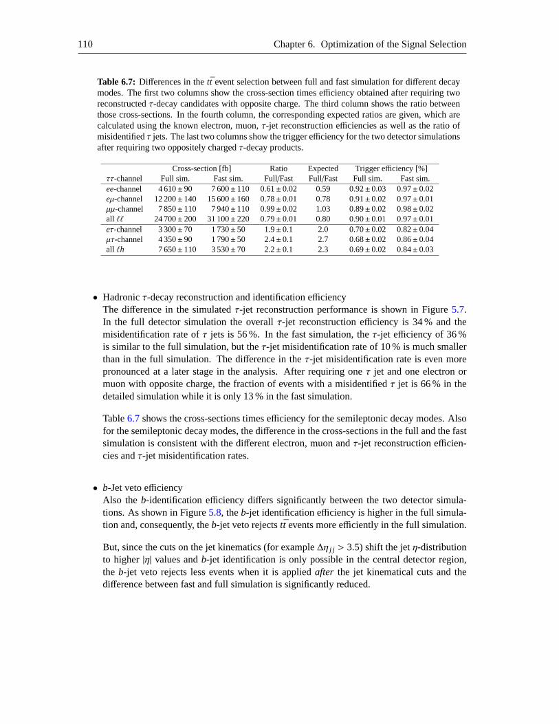
110 Chapter 6. Optimization of the Signal Selection
Table 6.7: Differences in thett event selection between full and fast simulation for different decaymodes. The first two columns show the cross-section times efficiency obtained after requiring tworeconstructedτ-decay candidates with opposite charge. The third column shows the ratio betweenthose cross-sections. In the fourth column, the corresponding expected ratios are given, which arecalculated using the known electron, muon,τ-jet reconstruction efficiencies as well as the ratio ofmisidentifiedτ jets. The last two columns show the trigger efficiency for the two detector simulationsafter requiring two oppositely chargedτ-decay products.
Cross-section [fb] Ratio Expected Trigger efficiency [%]ττ-channel Full sim. Fast sim. Full/Fast Full/Fast Full sim. Fast sim.ee-channel 4 610±90 7 600±110 0.61±0.02 0.59 0.92±0.03 0.97±0.02eµ-channel 12 200±140 15 600±160 0.78±0.01 0.78 0.91±0.02 0.97±0.01µµ-channel 7 850±110 7 940±110 0.99±0.02 1.03 0.89±0.02 0.98±0.02all ℓℓ 24 700±200 31 100±220 0.79±0.01 0.80 0.90±0.01 0.97±0.01eτ-channel 3 300±70 1 730±50 1.9±0.1 2.0 0.70±0.02 0.82±0.04µτ-channel 4 350±90 1 790±50 2.4±0.1 2.7 0.68±0.02 0.86±0.04all ℓh 7 650±110 3 530±70 2.2±0.1 2.3 0.69±0.02 0.84±0.03
• Hadronicτ-decay reconstruction and identification efficiencyThe difference in the simulatedτ-jet reconstruction performance is shown in Figure5.7.In the full detector simulation the overallτ-jet reconstruction efficiency is 34 % and themisidentification rate ofτ jets is 56 %. In the fast simulation, theτ-jet efficiency of 36 %is similar to the full simulation, but theτ-jet misidentification rate of 10 % is much smallerthan in the full simulation. The difference in theτ-jet misidentification rate is even morepronounced at a later stage in the analysis. After requiring oneτ jet and one electron ormuon with opposite charge, the fraction of events with a misidentifiedτ jet is 66 % in thedetailed simulation while it is only 13 % in the fast simulation.
Table6.7shows the cross-sections times efficiency for the semileptonic decay modes. Alsofor the semileptonic decay modes, the difference in the cross-sections in the full and the fastsimulation is consistent with the different electron, muon andτ-jet reconstruction efficien-cies andτ-jet misidentification rates.
• b-Jet veto efficiencyAlso the b-identification efficiency differs significantly between the two detector simula-tions. As shown in Figure5.8, theb-jet identification efficiency is higher in the full simula-tion and, consequently, theb-jet veto rejectstt events more efficiently in the full simulation.
But, since the cuts on the jet kinematics (for example∆η j j > 3.5) shift the jetη-distributionto higher|η| values andb-jet identification is only possible in the central detector region,the b-jet veto rejects less events when it is appliedafter the jet kinematical cuts and thedifference between fast and full simulation is significantly reduced.
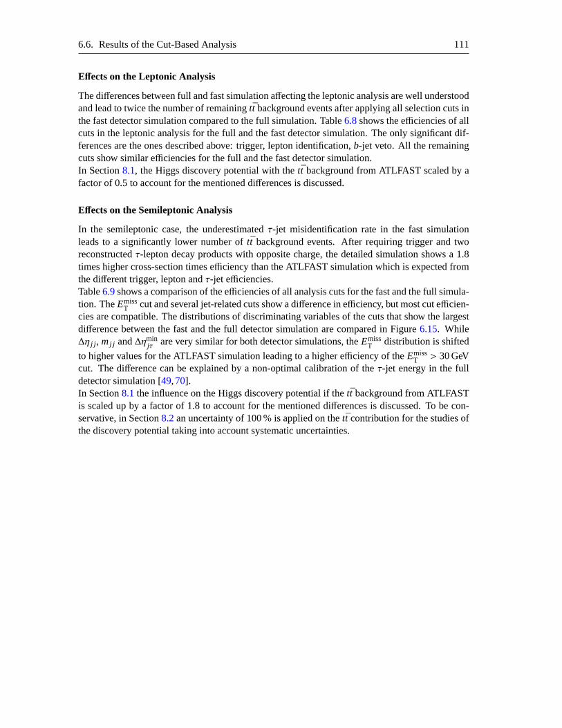
6.6. Results of the Cut-Based Analysis 111
Effects on the Leptonic Analysis
The differences between full and fast simulation affecting the leptonic analysis are well understoodand lead to twice the number of remainingtt background events after applying all selection cuts inthe fast detector simulation compared to the full simulation. Table6.8shows the efficiencies of allcuts in the leptonic analysis for the full and the fast detector simulation. The only significant dif-ferences are the ones described above: trigger, lepton identification,b-jet veto. All the remainingcuts show similar efficiencies for the full and the fast detector simulation.In Section8.1, the Higgs discovery potential with thett background from ATLFAST scaled by afactor of 0.5 to account for the mentioned differences is discussed.
Effects on the Semileptonic Analysis
In the semileptonic case, the underestimatedτ-jet misidentification rate in the fast simulationleads to a significantly lower number oftt background events. After requiring trigger and tworeconstructedτ-lepton decay products with opposite charge, the detailed simulation shows a 1.8times higher cross-section times efficiency than the ATLFAST simulation which is expected fromthe different trigger, lepton andτ-jet efficiencies.Table6.9shows a comparison of the efficiencies of all analysis cuts for the fast and the full simula-tion. TheEmiss
T cut and several jet-related cuts show a difference in efficiency, but most cut efficien-cies are compatible. The distributions of discriminating variables of the cuts thatshow the largestdifference between the fast and the full detector simulation are compared in Figure 6.15. While∆η j j , mj j and∆ηmin
jτ are very similar for both detector simulations, theEmissT distribution is shifted
to higher values for the ATLFAST simulation leading to a higher efficiency of theEmissT > 30 GeV
cut. The difference can be explained by a non-optimal calibration of theτ-jet energy in the fulldetector simulation [49,70].In Section8.1the influence on the Higgs discovery potential if thett background from ATLFASTis scaled up by a factor of 1.8 to account for the mentioned differences is discussed. To be con-servative, in Section8.2an uncertainty of 100 % is applied on thett contribution for the studies ofthe discovery potential taking into account systematic uncertainties.
112 Chapter 6. Optimization of the Signal Selection
Table 6.8: Cut efficiencies ontt events for the fast and the full detector simulation in the leptonicdecay channel. The values represent the cut efficiencies without applying the other cuts before.
Cut Efficiency (%)Fast sim. Full sim.
Trigger+ N(e, µ)=2 3.8±0.1 2.7±0.1
Opposite charge 97±0.3 96±1.1Emiss
T > 40 GeV 78±0.1 78±0.8∆φττ < 2.5 71±0.1 70±0.7χ1,2 = 0.0− 1.0 19±0.1 19±0.3mℓνT < 100 GeV 62±0.1 61±0.7N(jets)≥ 2 88±0.3 88±1.1η j1 × η j2 < 0 44±0.1 45±0.5∆η jτ > 0 24±0.1 24±0.4mj j > 600 GeV,∆η j j > 3.5 4.1±0.1 4.2±0.2∆φ j j < 2.2 51±0.1 53±0.6∆ηmin
jτ > 0.6 7.3±0.1 7.6±0.2∆ηmax
jτ > 1.5 27±0.1 28±0.5Central jet veto 37±0.1 35±0.5ptot
T < 30 GeV 38±0.1 40±0.5mττ = mH ± 15 GeV 5.3±0.1 5.4±0.2
b-jet veto 36±0.1 17±0.3
After mj j > 600 GeV,∆η j j > 3.5,η j1 × η j2 < 0,∆η jτ > 0 andCentral jet veto cut:b-jet veto 59±1.2 38±8.0

6.6. Results of the Cut-Based Analysis 113
Table 6.9: Cut efficiencies ontt events for the fast and the full detector simulation in the semileptonicdecay channel. The values represent the cut efficiencies without applying the other cuts before.
Cut Efficiency (%)Fast sim. Full sim.
Trigger+ N(e, µ)=1 25±0.1 19±0.1N(τ)=1 1.5±0.1 4.0±0.1Opposite charge 94±2.9 84±2.0
EmissT > 30 GeV 86±0.3 81±0.3∆φττ < 2.5 64±0.3 66±1.5χℓ,h = 0.0− 1.0 25±0.1 22±0.7mℓνT < 30 GeV 15±0.1 16±0.6N(jets)≥ 2 88±2.3 90±2.3η j1 × η j2 < 0 44±0.2 42±1.1∆η jτ > 0 25±0.2 22±0.8∆η j j > 3.6,mj j > 600 GeV 4.1±0.1 3.2±0.3∆φ j j < 2.7 76±0.3 76±1.6∆ηmin
jτ > 0.8 4.4±0.1 3.8±0.3∆ηmax
jτ > 1.5 27±0.2 23±0.8Central jet veto 35±0.2 26±0.1ptot
T < 40 GeV 50±0.2 50±1.2mττ = mH ± 15 GeV 6.4±0.1 6.5±0.4
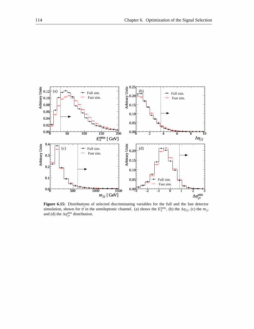
114 Chapter 6. Optimization of the Signal Selection
00 5050 100100 150150 2002000.000.00
0.020.02
0.040.04
0.060.06
0.080.08
0.100.10
0.120.12
EmissT [ GeV]EmissT [ GeV]
∆
Arb
itrar
yU
nits
Arb
itrar
yU
nits
Full sim.Fast sim.
(a)
00 22 44 66 88 10100.000.00
0.050.05
0.100.10
0.150.15
0.200.20
0.250.25
∆η j j∆η j j
Arb
itrar
yU
nits
Arb
itrar
yU
nits
Full sim.Fast sim.
(b)
00 500500 10001000 150015000.00.0
0.10.1
0.20.2
0.30.3
0.40.4
0.30
mj j [ GeV]mj j [ GeV]
Arb
itrar
yU
nits
Arb
itrar
yU
nits
Full sim.Fast sim.
(c)
-3-3 -2-2 -1-1 00 11 22 330.000.00
0.050.05
0.100.10
0.150.15
0.200.20
∆ηminjτ∆ηminjτ
Arb
itrar
yU
nits
Arb
itrar
yU
nits
Full sim.Fast sim.
(d)
Figure 6.15: Distributions of selected discriminating variables for the full and the fast detectorsimulation, shown fortt in the semileptonic channel. (a) shows theEmiss
T , (b) the∆η j j , (c) themj j
and (d) the∆ηminjτ distribution.
Chapter 7
Multivariate Analysis
In this chapter, the application of Multivariate Analysis (MVA) methods to the search for theHiggs boson is studied. Compared to the cut-based analysis presented in theprevious chapter,multivariate analysis methods may provide a better separation between the signal and backgroundby taking into account the information of all discriminating variables including their correlations.The advantages of MVA methods are introduced in Section7.1.For this study, the dedicated software package TMVA [71] has been used. The package containsa large collection of multivariate methods, from which the Fisher discriminant method, the pro-jective likelihood method, Boosted Decision Trees (BDT) and Artificial Neural Networks (ANN)have been selected to evaluate their performance. The principle of each of these methods is de-scribed very briefly in Section7.2. Further details can be found in many textbooks or in the TMVAUser guide [71].Before a given MVA method can be used to classify an event as signal- orbackground-like, it hasto be trained with events identified as signal or background. For this purpose Monte Carlo datahas been used.In Section7.3, the selection of events used for the training and in Section7.4the optimal selectionof discriminating variables is discussed. Section7.5 compares the performance of the differentmethods. The optimal results for theH → ττ decay search in the leptonic and semileptonic chan-nels are shown in Section7.6. Finally, in Section7.7 the stability of the results of the differentmultivariate methods is discussed.
7.1 Motivation
The cut-based event selection is characterized by a set of cuts applied sequentially on the discrim-inating variables. In case of correlations between these variables, their discriminating power isnot fully exploited. For example, consider the two arbitrary discriminating variablesx1 and x2.Signal (S) and background (B) events are distributed in the two dimensionalx1-x2 space as illus-trated in Figure7.1a. The discrimination between signal and background in the cut-based analysisis shown in Figure7.1b. Obviously, the selection using independent rectangular cuts does notprovide optimal separation.In contrast, MVA methods take into account correlations between the discriminating variables
115

116 Chapter 7. Multivariate Analysis
x1
x 2
B
S
Background events,B
Signal events,S(a)
x1
x 2
B
S
(b)
x1
x 2B
S
(c)
x1
x 2
B
S
(d)
x1
x 2
B
S
(e)
Figure 7.1: Examples for different signal and background classification strategies in two dimen-sions. The distribution of the events in the plane of the two discriminating variablesx1 and x2 isshown in (a). The discrimination can be made by (b) two rectangular cuts performed independentlyin each variable, (c) one linear diagonal cut or (d) a nonlinear boundary between the signal andbackground distributions. In (e) an extreme case of a very specific nonlinear boundary is shown.
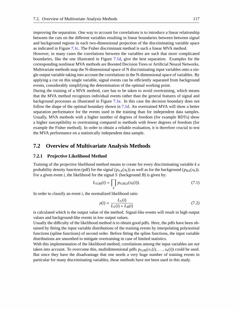
7.2. Overview of Multivariate Analysis Methods 117
improving the separation. One way to account for correlations is to introducea linear relationshipbetween the cuts on the different variables resulting in linear boundaries between between signaland background regions in each two-dimensional projection of the discriminating variable spaceas indicated in Figure7.1c. The Fisher discriminant method is such a linear MVA method.However, in many cases the correlations between the variables are such that more complicatedboundaries, like the one illustrated in Figure7.1d, give the best separation. Examples for thecorresponding nonlinear MVA methods are Boosted Decision Trees or Artificial Neural Networks.Multivariate methods map the N-dimensional space of N discriminating input variables onto a sin-gle output variable taking into account the correlations in the N-dimensional space of variables. Byapplying a cut on this single variable, signal events can be efficiently separated from backgroundevents, considerably simplifying the determination of the optimal working point.During the training of a MVA method, care has to be taken to avoid overtraining, which meansthat the MVA method recognizes individual events rather than the generalfeatures of signal andbackground processes as illustrated in Figure7.1e. In this case the decision boundary does notfollow the shape of the optimal boundary shown in7.1d. An overtrained MVA will show a betterseparation performance for the events used in the training than for independent data samples.Usually, MVA methods with a higher number of degrees of freedom (for example BDTs) showa higher susceptibility to overtraining compared to methods with fewer degreesof freedom (forexample the Fisher method). In order to obtain a reliable evaluation, it is therefore crucial to testthe MVA performance on a statistically independent data sample.
7.2 Overview of Multivariate Analysis Methods
7.2.1 Projective Likelihood Method
Training of the projective likelihood method means to create for every discriminating variablek aprobability density function (pdf) for the signal (pS,k(xk)) as well as for the background (pB,k(xk)).For a given eventi, the likelihood for the signalS (backgroundB) is given by:
LS(B)(i) =∏
k
pS(B),k(xk(i)). (7.1)
In order to classify an eventi, the normalized likelihood ratio
y(i) =LS(i)
LS(i) + LB(i)(7.2)
is calculated which is the output value of the method. Signal-like events will result in high outputvalues and background-like events in low output values.Usually the difficulty of the likelihood method is to obtain good pdfs. Here, the pdfs have beenob-tained by fitting the input variable distributions of the training events by interpolating polynomialfunctions (spline functions) of second order. Before fitting the spline functions, the input variabledistributions are smoothed to mitigate overtraining in case of limited statistics.With this implementation of the likelihood method, correlations among the input variables arenottaken into account. To overcome this, multidimensional pdfspS(B)(x1(i), . . . , xk(i)) could be used.But since they have the disadvantage that one needs a very huge numberof training events inparticular for many discriminating variables, these methods have not been used in this study.
118 Chapter 7. Multivariate Analysis
7.2.2 Fisher Discriminant Method
The Fisher Linear Discriminant analysis method [72], calculates the line in the multidimensionalspace of thek input variables that provides the best separation between signal and background.If signal and background events are projected to a line perpendicular tothe separation line, thedistance between their mean values is maximized and the variance of the signal as well as thebackground distribution is minimized.The output variable of the Fisher method is the projected coordinate and it is determined by alinear combination of the input variables,
y(i) = F0 +∑
k
Fkxk(i), (7.3)
where the Fisher coefficientsFk are given by:
Fk =
√NSNB
NS + NB
nvar∑
l=1
W−1kl (xS,l − xB,l) (7.4)
with Wkl being the sum of the covariant matricesCS,kl andCB,kl for signal and background respec-tively. xS(B),l denotes the mean of the signal (background) training event distributions.NS(B) is thenumber of signal (background) training events.By construction, the simple and robust Fisher method provides the optimum classification in caseof linearly correlated and Gaussian distributed input variables.
7.2.3 Artificial Neural Networks
The basic idea of an Artificial Neural Network (ANN) is motivated by the working principleof biological neural networks. As in biology, an ANN consists of a numberof interconnected“neurons”. The connections transfer the output of one neuron with a certain weight to the input ofanother neuron. Each neuron sums up the input values and calculates anoutput value accordingto a certain response function. By feeding the values of discriminating variables to input neurons,the state of the whole network is defined corresponding to the response ofa output neuron. If theANN is trained to distinguish between different input patterns, the output of the ANN can be usedto discriminate between them.ANNs are widely used for pattern recognition and a large collection of ANN implementationsexists. The type of network used in this analysis is a so-called feed-forward multilayer perceptronwhere the neurons are organized in layers and connections exist only between the outputs of onelayer and the inputs of the next layer. Figure7.2 shows the layout of such an ANN. The inputvalues are fed to the neurons in the input layer (“Layer 0”) and the output is formed by the singleneuron in the last layer (“Layer 3”). The neuron layers 1 and 2 are not accessible from the outsideand are therefore called hidden layers. The response function is usually a nonlinear function toenable the ANN to cope with nonlinear correlations. Here, the hyperbolic tangent function isused to describe the response of the neurons. The transfer function of the input neurons is 1.Each neuron is also connected to a “bias node” with constant output value1, which allows for anadditive constant in the network function.
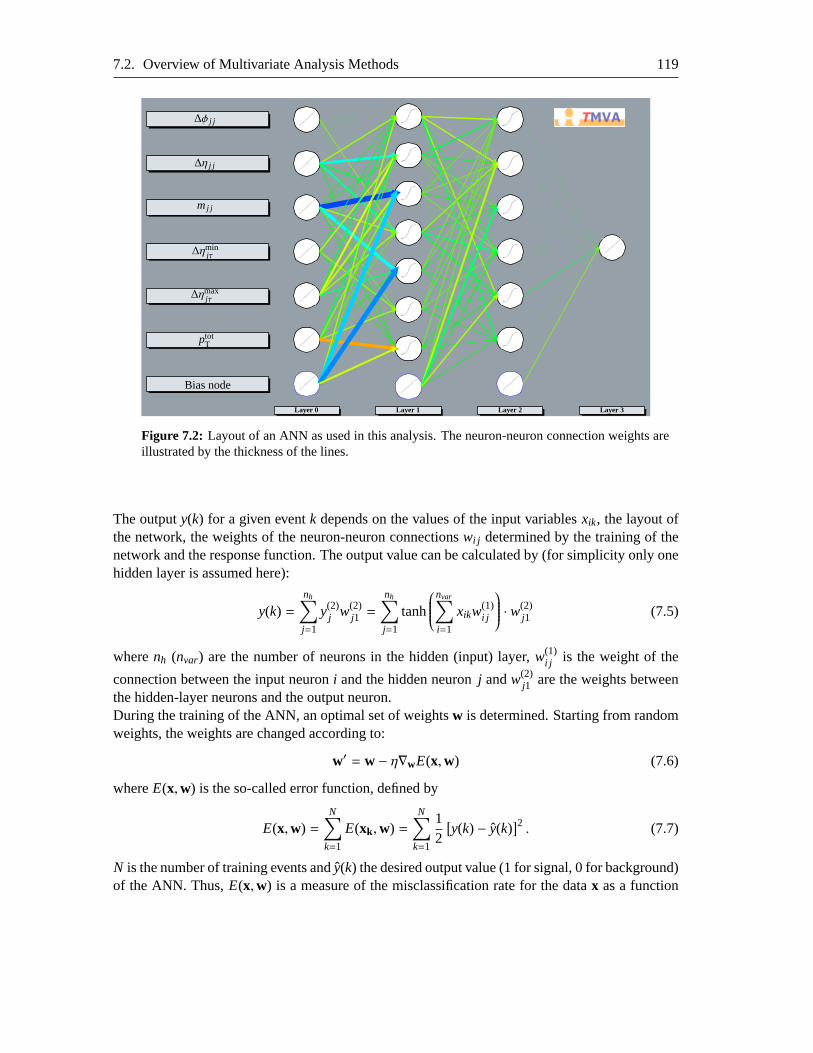
7.2. Overview of Multivariate Analysis Methods 119
∆φ j j
∆η j j
mj j
∆ηminjτ
∆ηmaxjτ
ptotT
Bias node
Layer 0 Layer 1 Layer 2 Layer 3
Figure 7.2: Layout of an ANN as used in this analysis. The neuron-neuron connection weights areillustrated by the thickness of the lines.
The outputy(k) for a given eventk depends on the values of the input variablesxik, the layout ofthe network, the weights of the neuron-neuron connectionswi j determined by the training of thenetwork and the response function. The output value can be calculated by (for simplicity only onehidden layer is assumed here):
y(k) =nh∑
j=1
y(2)j w(2)
j1 =
nh∑
j=1
tanh
nvar∑
i=1
xikw(1)i j
· w(2)j1 (7.5)
wherenh (nvar) are the number of neurons in the hidden (input) layer,w(1)i j is the weight of the
connection between the input neuroni and the hidden neuronj andw(2)j1 are the weights between
the hidden-layer neurons and the output neuron.During the training of the ANN, an optimal set of weightsw is determined. Starting from randomweights, the weights are changed according to:
w′ = w − η∇wE(x,w) (7.6)
whereE(x,w) is the so-called error function, defined by
E(x,w) =N∑
k=1
E(xk ,w) =N∑
k=1
12[
y(k) − y(k)]2. (7.7)
N is the number of training events and ˆy(k) the desired output value (1 for signal, 0 for background)of the ANN. Thus,E(x,w) is a measure of the misclassification rate for the datax as a function
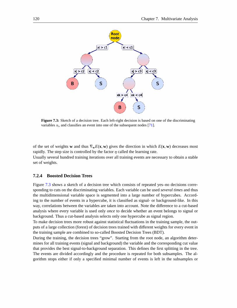
120 Chapter 7. Multivariate Analysis
Figure 7.3: Sketch of a decision tree. Each left-right decision is basedon one of the discriminatingvariablesxi , and classifies an event into one of the subsequent nodes [71].
of the set of weightsw and thus∇wE(x,w) gives the direction in whichE(x,w) decreases mostrapidly. The step size is controlled by the factorη called the learning rate.Usually several hundred training iterations over all training events are necessary to obtain a stableset of weights.
7.2.4 Boosted Decision Trees
Figure7.3 shows a sketch of a decision tree which consists of repeated yes–no decisions corre-sponding to cuts on the discriminating variables. Each variable can be usedseveral timesand thusthe multidimensional variable space is segmented into a large number of hypercubes. Accord-ing to the number of events in a hypercube, it is classified as signal- or background-like. In thisway, correlations between the variables are taken into account. Note the difference to a cut-basedanalysis where every variable is used onlyonceto decide whether an event belongs to signal orbackground. Thus a cut-based analysis selects only one hypercube as signal region.To make decision trees more robust against statistical fluctuations in the training sample, the out-puts of a large collection (forest) of decision trees trained with different weights for every event inthe training sample are combined to so-called Boosted Decision Trees (BDT).During the training, the decision trees “grow”. Starting from the root node, an algorithm deter-mines for all training events (signal and background) the variable and thecorresponding cut valuethat provides the best signal-to-background separation. This definesthe first splitting in the tree.The events are divided accordingly and the procedure is repeated forboth subsamples. The al-gorithm stops either if only a specified minimal number of events is left in the subsamples or
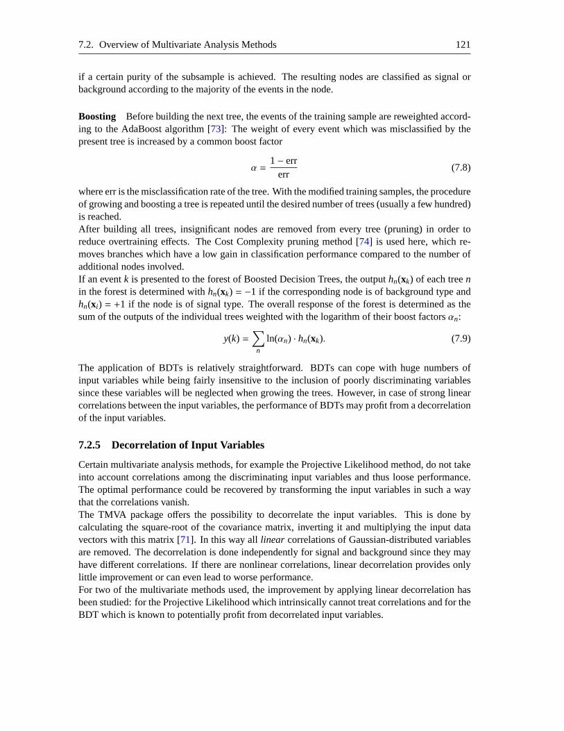
7.2. Overview of Multivariate Analysis Methods 121
if a certain purity of the subsample is achieved. The resulting nodes are classified as signal orbackground according to the majority of the events in the node.
Boosting Before building the next tree, the events of the training sample are reweighted accord-ing to the AdaBoost algorithm [73]: The weight of every event which was misclassified by thepresent tree is increased by a common boost factor
α =1− err
err(7.8)
where err is the misclassification rate of the tree. With the modified training samples, the procedureof growing and boosting a tree is repeated until the desired number of trees(usually a few hundred)is reached.After building all trees, insignificant nodes are removed from every tree(pruning) in order toreduce overtraining effects. The Cost Complexity pruning method [74] is used here, which re-moves branches which have a low gain in classification performance compared to the number ofadditional nodes involved.If an eventk is presented to the forest of Boosted Decision Trees, the outputhn(xk) of each treenin the forest is determined withhn(xk) = −1 if the corresponding node is of background type andhn(xi) = +1 if the node is of signal type. The overall response of the forest is determined as thesum of the outputs of the individual trees weighted with the logarithm of their boost factorsαn:
y(k) =∑
n
ln(αn) · hn(xk). (7.9)
The application of BDTs is relatively straightforward. BDTs can cope with huge numbers ofinput variables while being fairly insensitive to the inclusion of poorly discriminating variablessince these variables will be neglected when growing the trees. However,in case of strong linearcorrelations between the input variables, the performance of BDTs may profit from a decorrelationof the input variables.
7.2.5 Decorrelation of Input Variables
Certain multivariate analysis methods, for example the Projective Likelihood method, do not takeinto account correlations among the discriminating input variables and thus loose performance.The optimal performance could be recovered by transforming the input variables in such a waythat the correlations vanish.The TMVA package offers the possibility to decorrelate the input variables. This is done bycalculating the square-root of the covariance matrix, inverting it and multiplying the input datavectors with this matrix [71]. In this way all linear correlations of Gaussian-distributed variablesare removed. The decorrelation is done independently for signal and background since they mayhave different correlations. If there are nonlinear correlations, linear decorrelation provides onlylittle improvement or can even lead to worse performance.For two of the multivariate methods used, the improvement by applying linear decorrelation hasbeen studied: for the Projective Likelihood which intrinsically cannot treatcorrelations and for theBDT which is known to potentially profit from decorrelated input variables.
122 Chapter 7. Multivariate Analysis
7.3 Training of Multivariate Methods
For the training of multivariate methods, Monte Carlo data samples for signal and backgroundare necessary, which have to be independent of the data used for the evaluation of the analysisperformance. The number of events needed for an optimal training depends on the MVA methodand on the complexity of the discrimination between signal and background. Usually betweenseveral hundred and several ten thousand events are needed to obtain a good result.In order to obtain a sufficient number of background events for the training, only very loose pres-election cuts have been applied, much looser than those used for the cut optimization in Section6.Table7.1summarizes the preselection cut criteria used for the training and the testing ofthe MVAmethods. For the training events, decay products of twoτ-lepton candidates with opposite chargeand two forward jets in opposite detector hemispheres were required. No trigger cuts, noEmiss
Tcut, no central- andb-jet veto and only very loose cuts on the momentum fractionsχ1,2 have beenapplied.Due to the loose preselection cuts, the multidimensional distributions of discriminating variablesin the training can slightly differ from the event shapes on which the trained MVA methods areeventually applied. This leads to a loss of performance, which is also expected in the analysis ofreal data. The dependence of the performance of the MVA methods on thepreselection cuts andon the number of training events has been studied in Section7.7.4.An additional preselection cut is needed for thett background, which has been produced with theMC@NLO generator. During the generation of events, one has to avoid double counting of eventswhen matching parton showers to matrix elements. In MC@NLO this is done by introducingnegative “counter-events” to keep the cross-section right. Thus, about 13 % of thett events have anegative weight. Since negatively weighted events cannot be used in all MVA methods,tt eventswith negative weight have been excluded from the training. The distributions of the input variablesdo not change significantly if negatively weighted events are excluded.The training data statistics is further increased by using additional ATLFASTdata samples for theZ→ ττ background. An overview of the data samples used for the training is shown in Table7.3.
7.4 Selection of Input Variables
In the following, different sets of input variables have been tested in order to select the one withthe best separation of signal and background events in the leptonic decay channel. It is assumedthat the same variable selection will also provide the best signal-to-background separation for thesemileptonic decay channel. In principle, one can include all potential discriminating variables asan input to the MVA methods. However, care has to be taken to avoid the following problems:
• Correlation with the reconstructed Higgs boson massIn order to evaluate the Higgs boson discovery potential, it is crucial that the event selectioncriteria do not distort the reconstructedττmass distribution for signal and background. Forinput variables strongly correlated withmττ, the training can result in a mass dependentevent selection and thus change or shift themττ distribution. As an example for a stronglycorrelated variable, Figure7.4shows the correlation between the input variable∆φττ and theinvariant massmττ of theτ-lepton pair for signal andtt events. The resulting correlation of

7.4. Selection of Input Variables 123
Table 7.1: Event preselection criteria used for the training and performance tests of the multivariateanalysis methods. Full circles indicate that the cut was applied while the cuts marked with opencircles were not applied.
Training Testingℓℓ-Channel ℓh-Channel
Trigger ◦ • •N (e+ µ + τ) = 2 • • •Opposite lepton charge • • •N (jets)≥ 2 • • •∆ηmin
jτ > 0 • • •(η jet
1 · ηjet2 ) < 0 • • •
EmissT ◦ > 40 GeV > 30 GeV|∆φττ| < 2.9 • • •χ1,2 -2.0 ... 3.0 0 ... 1.0 0 ... 1.0mℓνT ◦ ◦ < 30 GeV∆η j j ◦ ◦ ◦∆φ j j ◦ ◦ ◦mj j ◦ ◦ ◦b-jet veto ◦ • ◦Central jet veto ◦ • •ptot
T ◦ ◦ ◦∆ηmin
jτ > 0 • • •∆ηmax
jτ > 0 • • •
124 Chapter 7. Multivariate Analysis
0 100 200 300 400 500
0.5
1.0
1.5
2.0
2.5<∆φττ>
mττ [ GeV ]
(a)
tt events
80 100 120 140 160
1.5
2.0
2.5
<∆φττ>
mττ [ GeV ]
(b)H → ττ eventsmH =120 GeV
Figure 7.4: Dependence of the mean of the∆φττ distribution on the reconstructed invariant massmττ, shown in (a) for thett background and in (b) for the signal.
the signal selection efficiency withmττ is shown in Figure7.5 for an ANN with∆φττ as aninput variable. Due to the strong mass correlation, the ANN provides a lowersuppression(higher selection efficiency) oftt events near the signal region (see Figure7.5a). Also forthe signal selection efficiency (see Figure7.5b) a mass sensitivity is observed, though notas pronounced as for thett events. The aim is to choose a mass independent selection.The correlation of the output of each MVA method with the reconstructedmττ has beentested for each set of input variables. In case of a significant correlation with mττ, thecorresponding set of input variables has not been used. Also nonlinear correlations havebeen taken into account by looking at the resulting dependencies and accepting only thosewhere no significant correlation is observed.
• Weak input variablesInput variables providing only weak separation between signal and background are calledweak variables. Depending on the multivariate method, the inclusion of weak variables canlead to a loss of performance.
• Strongly correlated input variablesUsing strongly correlated input variables can also lead to a loss of performance of certainMVA methods. Instead of rejecting strongly correlated variables, decorrelation of the inputvariables can be used. For MVA methods known to be sensitive to the correlation of inputvariables (Projective Likelihood, Boosted Decision Trees), the benefitof applying lineardecorrelation (see Page121) has been studied.
The input variables have been selected such that the above problems areavoided. Several sets ofinput variables have been tested, as summarized in Table7.2. The selection of the optimal set wasperformed in three steps:
1. In order to avoid sensitivity tomττ, only input variables without mass correlation have beenused. For this purpose, the mass correlation of all potential input variables has been deter-mined for the signal as well as for the two most important background processes,Z→ ττ
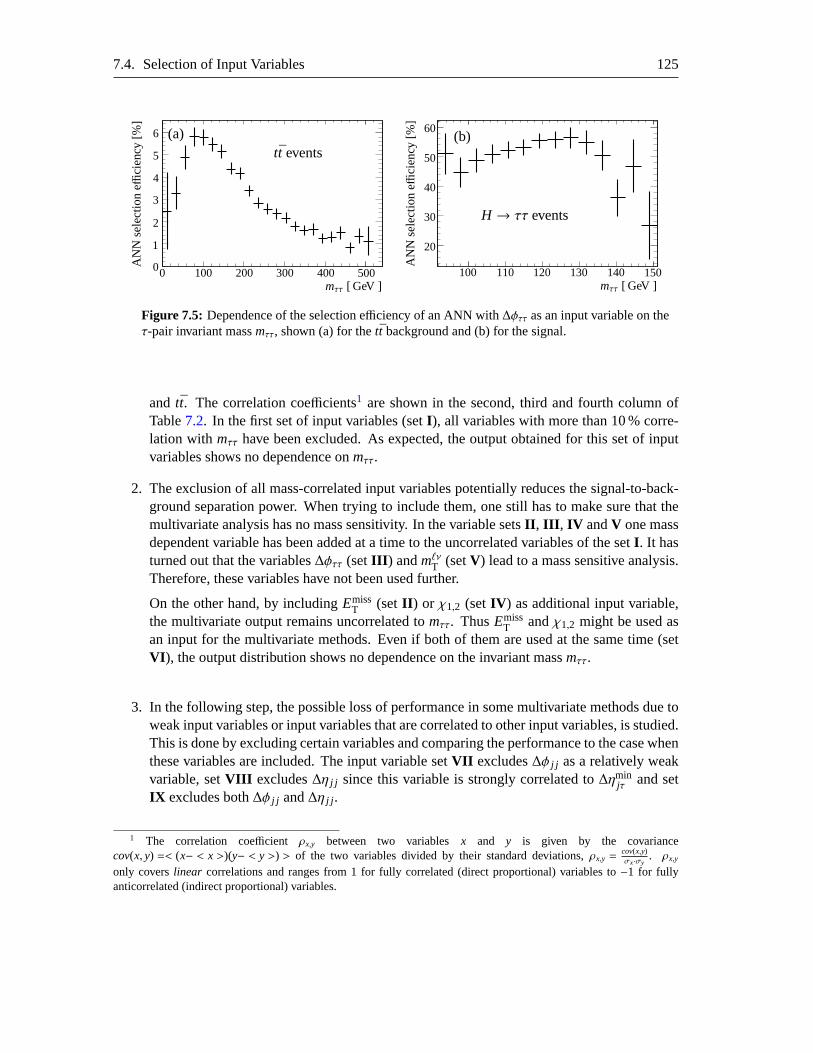
7.4. Selection of Input Variables 125
00
1
2
3
4
5
6
100 200 300 400 500
AN
Nse
lect
ion
effici
ency
[%]
mττ [ GeV ]
(a)tt events
20
30
40
50
60
100 110 120 130 140 150
AN
Nse
lect
ion
effici
ency
[%]
mττ [ GeV ]
(b)
H → ττ events
Figure 7.5: Dependence of the selection efficiency of an ANN with∆φττ as an input variable on theτ-pair invariant massmττ, shown (a) for thett background and (b) for the signal.
and tt. The correlation coefficients1 are shown in the second, third and fourth column ofTable7.2. In the first set of input variables (setI ), all variables with more than 10 % corre-lation with mττ have been excluded. As expected, the output obtained for this set of inputvariables shows no dependence onmττ.
2. The exclusion of all mass-correlated input variables potentially reduces the signal-to-back-ground separation power. When trying to include them, one still has to make sure that themultivariate analysis has no mass sensitivity. In the variable setsII , III , IV andV one massdependent variable has been added at a time to the uncorrelated variablesof the setI . It hasturned out that the variables∆φττ (setIII ) andmℓνT (setV) lead to a mass sensitive analysis.Therefore, these variables have not been used further.
On the other hand, by includingEmissT (setII ) or χ1,2 (setIV ) as additional input variable,
the multivariate output remains uncorrelated tomττ. ThusEmissT andχ1,2 might be used as
an input for the multivariate methods. Even if both of them are used at the sametime (setVI ), the output distribution shows no dependence on the invariant massmττ.
3. In the following step, the possible loss of performance in some multivariate methods due toweak input variables or input variables that are correlated to other inputvariables, is studied.This is done by excluding certain variables and comparing the performanceto the case whenthese variables are included. The input variable setVII excludes∆φ j j as a relatively weakvariable, setVIII excludes∆η j j since this variable is strongly correlated to∆ηmin
jτ and setIX excludes both∆φ j j and∆η j j .
1 The correlation coefficient ρx,y between two variablesx and y is given by the covariancecov(x, y) =< (x− < x >)(y− < y >) > of the two variables divided by their standard deviations,ρx,y =
cov(x,y)σx·σy
. ρx,y
only coverslinear correlations and ranges from 1 for fully correlated (direct proportional) variables to−1 for fullyanticorrelated (indirect proportional) variables.
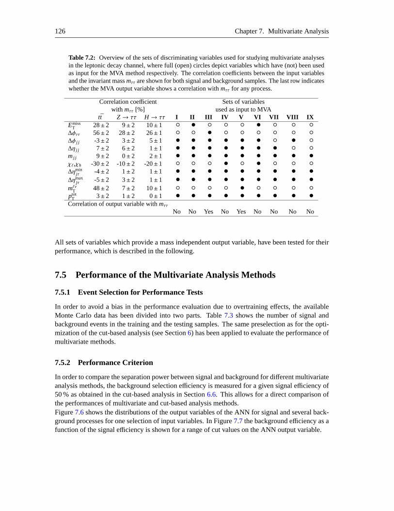
126 Chapter 7. Multivariate Analysis
Table 7.2: Overview of the sets of discriminating variables used for studying multivariate analysesin the leptonic decay channel, where full (open) circles depict variables which have (not) been usedas input for the MVA method respectively. The correlation coefficients between the input variablesand the invariant massmττ are shown for both signal and background samples. The last row indicateswhether the MVA output variable shows a correlation withmττ for any process.
Correlation coefficient Sets of variableswith mττ [%] used as input to MVA
tt Z→ ττ H → ττ I II III IV V VI VII VIII IXEmiss
T 28± 2 9±2 10± 1 ◦ • ◦ ◦ ◦ • ◦ ◦ ◦∆φττ 56± 2 28±2 26± 1 ◦ ◦ • ◦ ◦ ◦ ◦ ◦ ◦∆φ j j -3± 2 3±2 5± 1 • • • • • • ◦ • ◦∆η j j 7± 2 6±2 1± 1 • • • • • • • ◦ ◦mj j 9± 2 0±2 2± 1 • • • • • • • • •χℓ,χh -30± 2 -10±2 -20± 1 ◦ ◦ ◦ • ◦ • ◦ ◦ ◦∆ηmin
jτ -4± 2 1±2 1± 1 • • • • • • • • •∆ηmax
jτ -5± 2 3±2 1± 1 • • • • • • • • •mℓνT 48± 2 7±2 10± 1 ◦ ◦ ◦ ◦ • ◦ ◦ ◦ ◦ptot
T 3± 2 1±2 0± 1 • • • • • • • • •Correlation of output variable withmττ
No No Yes No Yes No No No No
All sets of variables which provide a mass independent output variable, have been tested for theirperformance, which is described in the following.
7.5 Performance of the Multivariate Analysis Methods
7.5.1 Event Selection for Performance Tests
In order to avoid a bias in the performance evaluation due to overtraining effects, the availableMonte Carlo data has been divided into two parts. Table7.3 shows the number of signal andbackground events in the training and the testing samples. The same preselection as for the opti-mization of the cut-based analysis (see Section6) has been applied to evaluate the performance ofmultivariate methods.
7.5.2 Performance Criterion
In order to compare the separation power between signal and background for different multivariateanalysis methods, the background selection efficiency is measured for a given signal efficiency of50 % as obtained in the cut-based analysis in Section6.6. This allows for a direct comparison ofthe performances of multivariate and cut-based analysis methods.Figure7.6shows the distributions of the output variables of the ANN for signal and several back-ground processes for one selection of input variables. In Figure7.7the background efficiency as afunction of the signal efficiency is shown for a range of cut values on the ANN output variable.
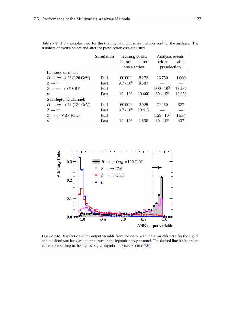
7.5. Performance of the Multivariate Analysis Methods 127
Table 7.3: Data samples used for the training of multivariate methods and for the analysis. Thenumbers of events before and after the preselection cuts arelisted.
Simulation Training events Analysis eventsbefore after before after
preselection preselectionLeptonic channel:H → ττ→ ℓℓ (120 GeV) Full 60 000 8 272 26 750 1 660Z→ ττ Fast 9.7 · 106 9 687 — —Z→ ττ→ ℓℓ VBF Full — — 990· 103 15 260tt Fast 10· 106 13 460 80· 106 16 650Semileptonic channel:H → ττ→ ℓh (120 GeV) Full 60 000 2 928 72 250 627Z→ ττ Fast 9.7 · 106 13 412 — —Z→ ττ VBF Filter Full — — 1.28 · 106 1 554tt Fast 10· 106 1 896 80· 106 437
-1.0-1.0 -0.5-0.50.0 0.00.0 0.0
0.10.1
0.20.2
0.30.3
0.50.5 1.01.0
Arb
itrar
yU
nits
Arb
itrar
yU
nits
Z→ ττ EW
tt
ANN output variableANN output variable
Z→ ττ QCD
H → ττ (mH =120 GeV)
Figure 7.6: Distribution of the output variable from the ANN with input variable setI for the signaland the dominant background processes in the leptonic decaychannel. The dashed line indicates thecut value resulting in the highest signal significance (see Section7.6).
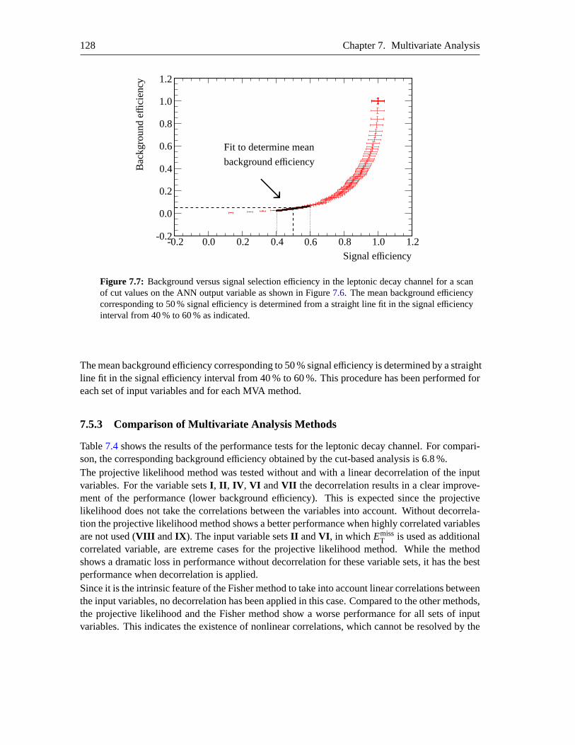
128 Chapter 7. Multivariate Analysis
-0.2-0.2
0.0
0.0
0.2
0.2
0.4
0.4
0.6
0.6
0.8
0.8
1.0
1.0
1.2
1.2Signal efficiency
Bac
kgro
und
effici
ency
Fit to determine mean
background efficiency
ց
Figure 7.7: Background versus signal selection efficiency in the leptonic decay channel for a scanof cut values on the ANN output variable as shown in Figure7.6. The mean background efficiencycorresponding to 50 % signal efficiency is determined from a straight line fit in the signal efficiencyinterval from 40 % to 60 % as indicated.
The mean background efficiency corresponding to 50 % signal efficiency is determined by a straightline fit in the signal efficiency interval from 40 % to 60 %. This procedure has been performed foreach set of input variables and for each MVA method.
7.5.3 Comparison of Multivariate Analysis Methods
Table7.4shows the results of the performance tests for the leptonic decay channel.For compari-son, the corresponding background efficiency obtained by the cut-based analysis is 6.8 %.The projective likelihood method was tested without and with a linear decorrelation of the inputvariables. For the variable setsI , II , IV , VI andVII the decorrelation results in a clear improve-ment of the performance (lower background efficiency). This is expected since the projectivelikelihood does not take the correlations between the variables into account.Without decorrela-tion the projective likelihood method shows a better performance when highly correlated variablesare not used (VIII andIX ). The input variable setsII andVI , in whichEmiss
T is used as additionalcorrelated variable, are extreme cases for the projective likelihood method.While the methodshows a dramatic loss in performance without decorrelation for these variable sets, it has the bestperformance when decorrelation is applied.Since it is the intrinsic feature of the Fisher method to take into account linear correlations betweenthe input variables, no decorrelation has been applied in this case. Compared to the other methods,the projective likelihood and the Fisher method show a worse performance for all sets of inputvariables. This indicates the existence of nonlinear correlations, which cannot be resolved by the
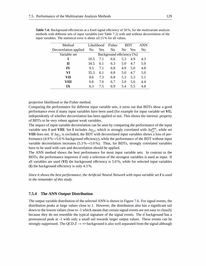
7.5. Performance of the Multivariate Analysis Methods 129
Table 7.4: Background efficiencies at a fixed signal efficiency of 50 %, for the multivariate analysismethods with different sets of input variables (see Table7.2) with and without decorrelation of theinput variables. The statistical error is about±0.15 % for all values.
Method Likelihood Fisher BDT ANNDecorrelation applied No Yes No No Yes No
Variable set Background efficiency [%]I 10.5 7.1 6.6 5.3 4.9 4.3II 34.5 6.1 6.3 5.0 4.7 5.0IV 9.5 7.1 6.8 4.9 5.0 4.8VI 35.3 6.1 6.8 5.0 4.7 5.0VII 8.6 7.3 6.8 5.3 5.3 5.1VIII 6.6 7.6 6.7 5.0 5.6 4.4IX 6.3 7.5 6.9 5.4 5.5 4.8
projective likelihood or the Fisher method.Comparing the performance for different input variable sets, it turns out that BDTs show a goodperformance even if many input variables have been used (for example for input variable setVI ),independently of whether decorrelation has been applied or not. This shows the intrinsic propertyof BDTs to be very robust against weak variables.The impact of input variable decorrelation can be seen by comparing the performance of the inputvariable setsI andVIII . SetI includes∆η j j , which is strongly correlated with∆ηmin
jτ , while setVIII does not. If∆η j j is excluded, the BDT with decorrelated input variables shows a loss of per-formance (4.9 %→5.6 % background efficiency), while the performance of the BDT without inputvariable decorrelation increases (5.3 %→5.0 %). Thus, for BDTs, strongly correlated variableshave to be used with care and decorrelation should be applied.The ANN method shows the best performance for most input variable sets.In contrast to theBDTs, the performance improves if only a selection of the strongest variables is used as input. Ifall variables are used (VI ) the background efficiency is 5.0 %, while for selected input variables(I ) the background efficiency is only 4.3 %.
Since it shows the best performance, the Artificial Neural Network with input variable setI is usedin the remainder of this study.
7.5.4 The ANN Output Distribution
The output variable distribution of the selected ANN is shown in Figure7.6. For signal events, thedistribution peaks at large values close to 1. However, the distribution also has a significant taildown to the lowest values close to -1 which means that certain signal events are not easy to classifybecause they do not resemble the typical signature of the signal events. The tt background has apronounced peak at -1 with only a small tail towards larger output values.These events can bestrongly suppressed. The QCDZ→ ττ background is also well separated from the signal although
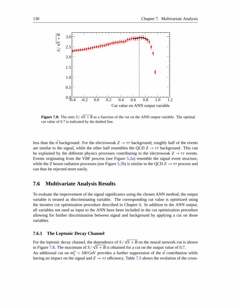
130 Chapter 7. Multivariate Analysis
-0.4 -0.20.0 0.0 0.2 0.4
0.5
0.6 0.8
1.0
1.0 1.2
1.5
2.0
2.5
3.0
S/√
S+
B
Cut value on ANN output variable
Figure 7.8: The ratioS/√
S + B as a function of the cut on the ANN output variable. The optimalcut value of 0.7 is indicated by the dashed line.
less than thett background. For the electroweakZ→ ττ background, roughly half of the eventsare similar to the signal, while the other half resembles the QCDZ→ ττ background. This canbe explained by the different physics processes contributing to the electroweakZ→ ττ events.Events originating from the VBF process (see Figure5.2a) resemble the signal event structure,while theZ boson radiation processes (see Figure5.2b) is similar to the QCDZ→ ττ process andcan thus be rejected more easily.
7.6 Multivariate Analysis Results
To evaluate the improvement of the signal significance using the chosen ANNmethod, the outputvariable is treated as discriminating variable. The corresponding cut valueis optimized usingthe iterative cut optimization procedure described in Chapter6. In addition to the ANN output,all variables not used as input to the ANN have been included in the cut optimization procedureallowing for further discrimination between signal and background by applying a cut on thosevariables.
7.6.1 The Leptonic Decay Channel
For the leptonic decay channel, the dependence ofS/√
S + B on the neural network cut is shownin Figure7.8. The maximum ofS/
√S + B is obtained for a cut on the output value of 0.7.
An additional cut onmℓνT < 100 GeV provides a further suppression of thett contribution whilehaving no impact on the signal andZ→ ττ efficiency. Table7.5shows the evolution of the cross-
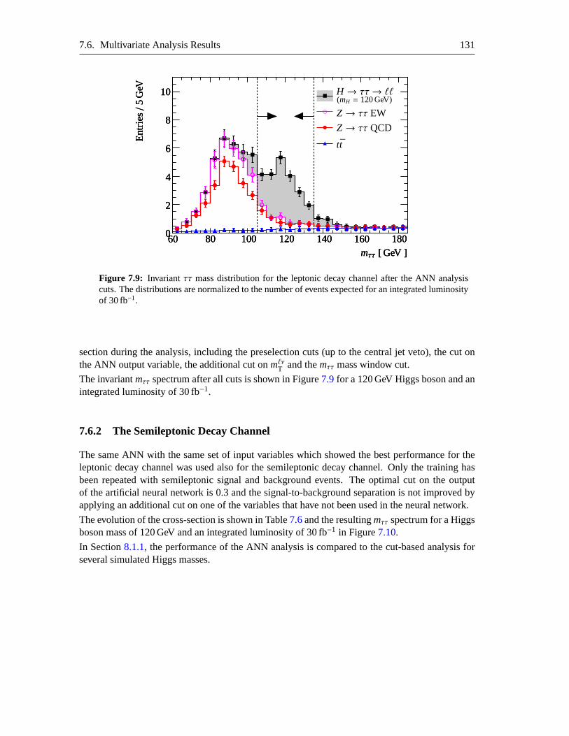
7.6. Multivariate Analysis Results 131
000
222
444
666
888
101010
606060 808080 100100100 120120120 140140140 160160160 180180180
Z→ ττ EW
tt
mττ [ GeV ]mττ [ GeV ]mττ [ GeV ]
Z→ ττ QCDE
ntrie
s/5
GeV
Ent
ries/
5G
eVE
ntrie
s/5
GeV H → ττ→ ℓℓ
(mH = 120 GeV)
Figure 7.9: Invariantττ mass distribution for the leptonic decay channel after the ANN analysiscuts. The distributions are normalized to the number of events expected for an integrated luminosityof 30 fb−1.
section during the analysis, including the preselection cuts (up to the centraljet veto), the cut onthe ANN output variable, the additional cut onmℓνT and themττ mass window cut.
The invariantmττ spectrum after all cuts is shown in Figure7.9for a 120 GeV Higgs boson and anintegrated luminosity of 30 fb−1.
7.6.2 The Semileptonic Decay Channel
The same ANN with the same set of input variables which showed the best performance for theleptonic decay channel was used also for the semileptonic decay channel.Only the training hasbeen repeated with semileptonic signal and background events. The optimalcut on the outputof the artificial neural network is 0.3 and the signal-to-background separation is not improved byapplying an additional cut on one of the variables that have not been used in the neural network.
The evolution of the cross-section is shown in Table7.6and the resultingmττ spectrum for a Higgsboson mass of 120 GeV and an integrated luminosity of 30 fb−1 in Figure7.10.
In Section8.1.1, the performance of the ANN analysis is compared to the cut-based analysisforseveral simulated Higgs masses.
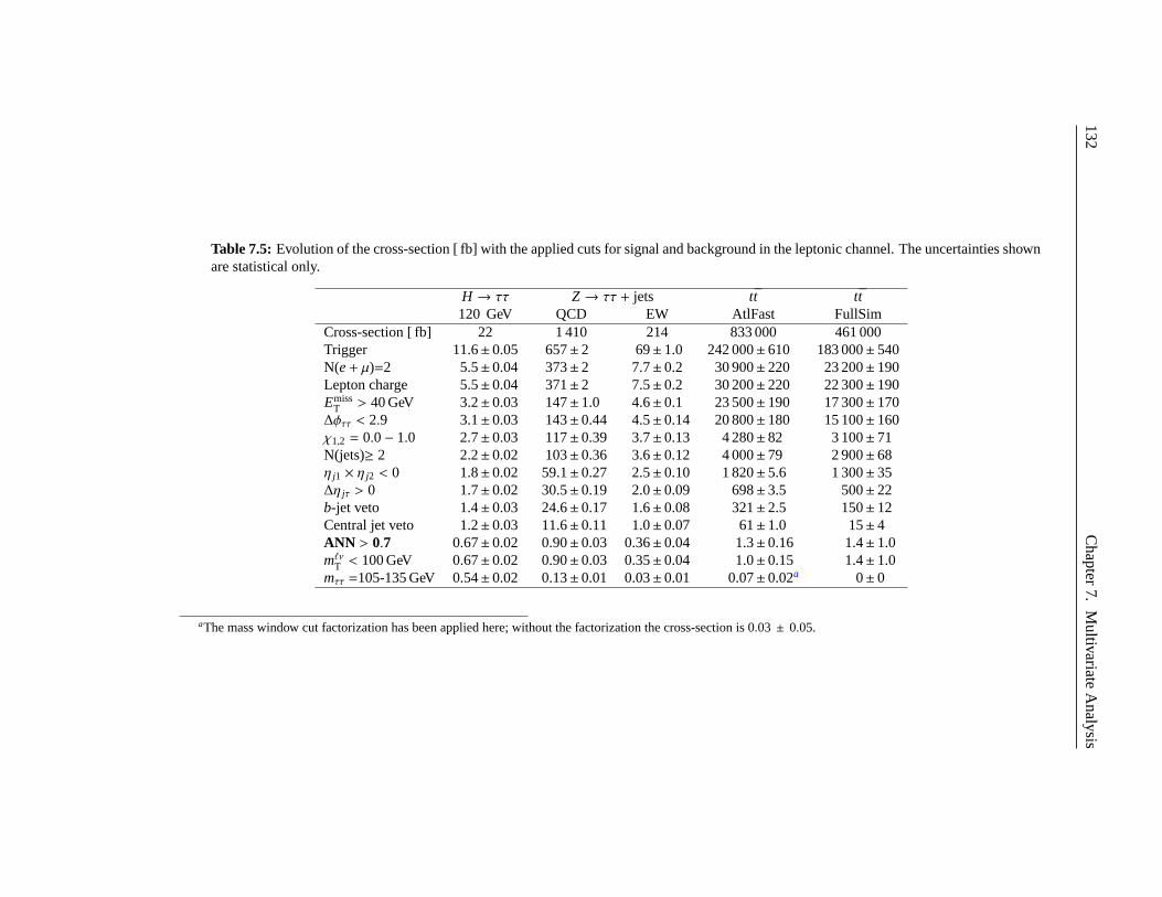
132C
hapter7.
Multivariate
Analysis
Table 7.5: Evolution of the cross-section [ fb] with the applied cuts for signal and background in the leptonic channel. The uncertainties shownare statistical only.
H → ττ Z→ ττ + jets tt tt120 GeV QCD EW AtlFast FullSim
Cross-section [ fb] 22 1 410 214 833 000 461 000Trigger 11.6±0.05 657±2 69± 1.0 242 000± 610 183 000± 540N(e+ µ)=2 5.5±0.04 373±2 7.7± 0.2 30 900± 220 23 200± 190Lepton charge 5.5±0.04 371±2 7.5± 0.2 30 200± 220 22 300± 190Emiss
T > 40 GeV 3.2±0.03 147±1.0 4.6± 0.1 23 500± 190 17 300± 170∆φττ < 2.9 3.1±0.03 143±0.44 4.5± 0.14 20 800± 180 15 100± 160χ1,2 = 0.0− 1.0 2.7±0.03 117±0.39 3.7± 0.13 4 280± 82 3 100± 71N(jets)≥ 2 2.2±0.02 103±0.36 3.6± 0.12 4 000± 79 2 900± 68η j1 × η j2 < 0 1.8±0.02 59.1±0.27 2.5± 0.10 1 820± 5.6 1 300± 35∆η jτ > 0 1.7±0.02 30.5±0.19 2.0± 0.09 698± 3.5 500± 22b-jet veto 1.4±0.03 24.6±0.17 1.6± 0.08 321± 2.5 150± 12Central jet veto 1.2±0.03 11.6±0.11 1.0± 0.07 61± 1.0 15± 4ANN > 0.7 0.67±0.02 0.90±0.03 0.36± 0.04 1.3± 0.16 1.4± 1.0mℓνT < 100 GeV 0.67±0.02 0.90±0.03 0.35± 0.04 1.0± 0.15 1.4± 1.0mττ =105-135 GeV 0.54±0.02 0.13±0.01 0.03± 0.01 0.07± 0.02a 0± 0
aThe mass window cut factorization has been applied here; without the factorization the cross-section is 0.03 ± 0.05.
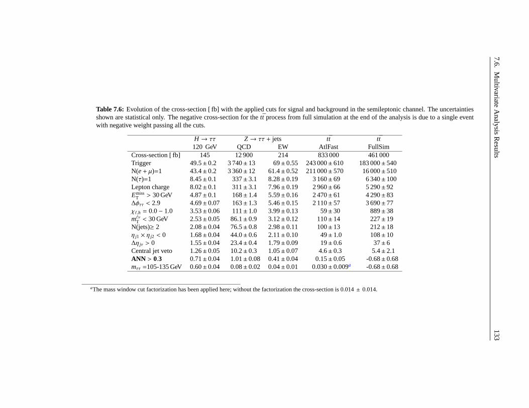
7.6.M
ultivariateA
nalysisR
esults133
Table 7.6: Evolution of the cross-section [ fb] with the applied cuts for signal and background in the semileptonic channel. The uncertaintiesshown are statistical only. The negative cross-section forthe tt process from full simulation at the end of the analysis is dueto a single eventwith negative weight passing all the cuts.
H → ττ Z→ ττ + jets tt tt120 GeV QCD EW AtlFast FullSim
Cross-section [ fb] 145 12 900 214 833 000 461 000Trigger 49.5± 0.2 3 740± 13 69± 0.55 243 000± 610 183 000±540N(e+ µ)=1 43.4± 0.2 3 360± 12 61.4± 0.52 211 000± 570 16 000±510N(τ)=1 8.45± 0.1 337± 3.1 8.28± 0.19 3 160± 69 6 340±100Lepton charge 8.02± 0.1 311± 3.1 7.96± 0.19 2 960± 66 5 290±92Emiss
T > 30 GeV 4.87± 0.1 168± 1.4 5.59± 0.16 2 470± 61 4 290±83∆φττ < 2.9 4.69± 0.07 163± 1.3 5.46± 0.15 2 110± 57 3 690±77χℓ,h = 0.0− 1.0 3.53± 0.06 111± 1.0 3.99± 0.13 59± 30 889±38mℓνT < 30 GeV 2.53± 0.05 86.1± 0.9 3.12± 0.12 110± 14 227±19N(jets)≥ 2 2.08± 0.04 76.5± 0.8 2.98± 0.11 100± 13 212±18η j1 × η j2 < 0 1.68± 0.04 44.0± 0.6 2.11± 0.10 49± 1.0 108±10∆η jτ > 0 1.55± 0.04 23.4± 0.4 1.79± 0.09 19± 0.6 37±6Central jet veto 1.26± 0.05 10.2± 0.3 1.05± 0.07 4.6± 0.3 5.4±2.1ANN > 0.3 0.71± 0.04 1.01± 0.08 0.41± 0.04 0.15± 0.05 -0.68±0.68mττ =105-135 GeV 0.60± 0.04 0.08± 0.02 0.04± 0.01 0.030± 0.009a -0.68±0.68
aThe mass window cut factorization has been applied here; without the factorization the cross-section is 0.014 ± 0.014.

134 Chapter 7. Multivariate Analysis
000
222
444
666
888
101010
121212
606060 808080 100100100 120120120 140140140 160160160 180180180
Z→ ττ QCD
Z→ ττ EW
tt
mττ [ GeV ]mττ [ GeV ]mττ [ GeV ]
Ent
ries/
5G
eVE
ntrie
s/5
GeV
Ent
ries/
5G
eV
H → ττ→ ℓh(mH = 120 GeV)
Figure 7.10: Invariantττ mass distribution for the semileptonic decay channel afterthe ANN anal-ysis cuts. The distributions are normalized to the number ofevents expected for an integrated lumi-nosity of 30 fb−1.
7.7 Systematic Tests
In this section several subjects specific to the performance and the stability of MVA methods arestudied: the separate treatment of the two different background types, the influence of a differentevent preselection for the training, the number of events used for the training, the ANN architec-ture, the number of training cycles and the learning rate. Finally, the influence of the MVA methodon the invariantττmass distribution is studied.
7.7.1 Separate Treatment of Backgrounds
In the described analysis, a mixture of the two main background processesZ→ ττ andtt weightedaccording to their cross-sections was used for the training of the MVA methods. Another possi-bility is to train one MVA method for every background process separately since in general theinput variables are differently distributed for different background processes. Examples are thetransverse massmℓνT (Figure5.20) or the visible momentum fractionsχ1,2 (Figure5.17). In thesecases, separate treatment of the backgrounds could provide better separation. Another advantageof treating the backgrounds separately is the possibility to use different sets of input variables forthe rejection of different backgrounds.A disadvantage is the need for several MVA instances. To suppress allbackground contributions,cuts are applied on the output variables of each MVA instance. This leads toa loss of performancesince the output variables are usually correlated.An ANN has been used to suppress theZ→ ττ and tt background. For discriminating between
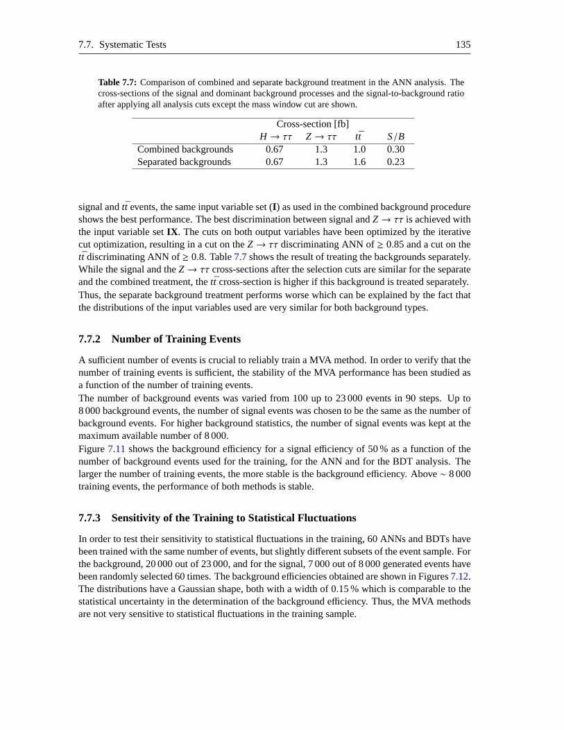
7.7. Systematic Tests 135
Table 7.7: Comparison of combined and separate background treatment in the ANN analysis. Thecross-sections of the signal and dominant background processes and the signal-to-background ratioafter applying all analysis cuts except the mass window cut are shown.
Cross-section [fb]H → ττ Z→ ττ tt S/B
Combined backgrounds 0.67 1.3 1.0 0.30Separated backgrounds 0.67 1.3 1.6 0.23
signal andtt events, the same input variable set (I ) as used in the combined background procedureshows the best performance. The best discrimination between signal andZ→ ττ is achieved withthe input variable setIX . The cuts on both output variables have been optimized by the iterativecut optimization, resulting in a cut on theZ→ ττ discriminating ANN of≥ 0.85 and a cut on thett discriminating ANN of≥ 0.8. Table7.7shows the result of treating the backgrounds separately.While the signal and theZ→ ττ cross-sections after the selection cuts are similar for the separateand the combined treatment, thett cross-section is higher if this background is treated separately.Thus, the separate background treatment performs worse which can beexplained by the fact thatthe distributions of the input variables used are very similar for both background types.
7.7.2 Number of Training Events
A sufficient number of events is crucial to reliably train a MVA method. In order to verify that thenumber of training events is sufficient, the stability of the MVA performance has been studied asa function of the number of training events.The number of background events was varied from 100 up to 23 000 events in 90 steps. Up to8 000 background events, the number of signal events was chosen to bethe same as the number ofbackground events. For higher background statistics, the number of signal events was kept at themaximum available number of 8 000.Figure7.11shows the background efficiency for a signal efficiency of 50 % as a function of thenumber of background events used for the training, for the ANN and forthe BDT analysis. Thelarger the number of training events, the more stable is the background efficiency. Above∼ 8 000training events, the performance of both methods is stable.
7.7.3 Sensitivity of the Training to Statistical Fluctuations
In order to test their sensitivity to statistical fluctuations in the training, 60 ANNsand BDTs havebeen trained with the same number of events, but slightly different subsets of the event sample. Forthe background, 20 000 out of 23 000, and for the signal, 7 000 out of8 000 generated events havebeen randomly selected 60 times. The background efficiencies obtained are shown in Figures7.12.The distributions have a Gaussian shape, both with a width of 0.15 % which is comparable to thestatistical uncertainty in the determination of the background efficiency. Thus, the MVA methodsare not very sensitive to statistical fluctuations in the training sample.
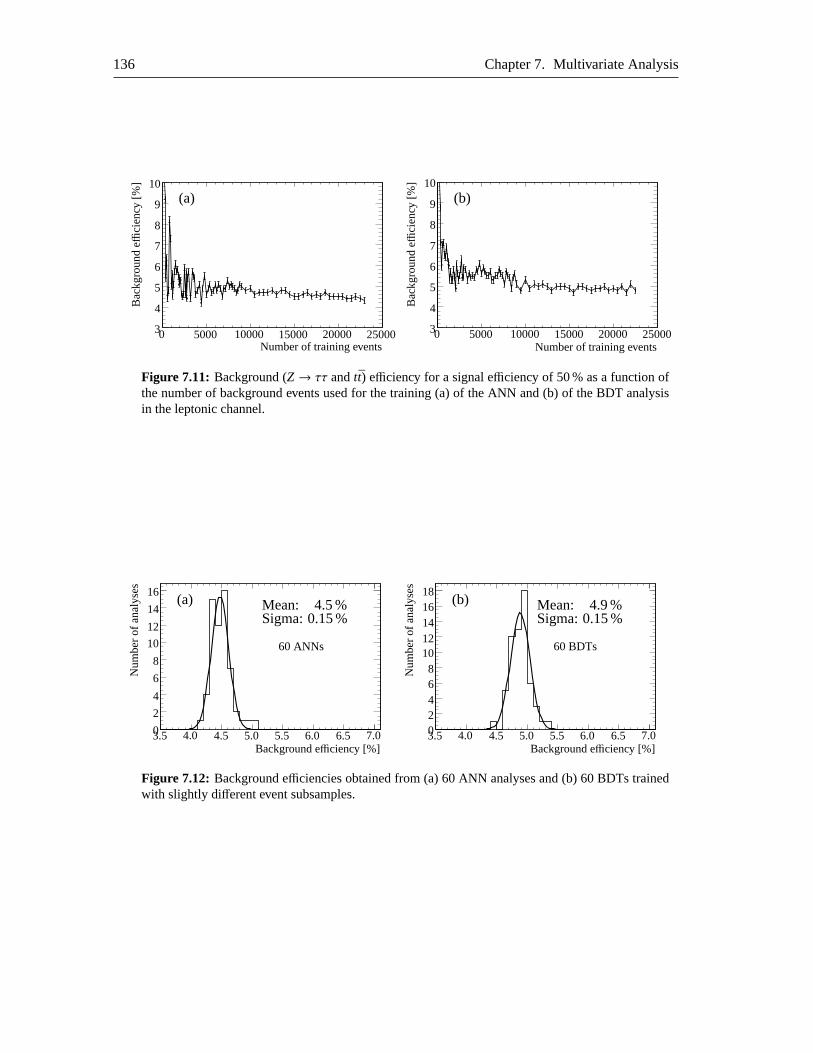
136 Chapter 7. Multivariate Analysis
03
4
5
6
7
8
9
10
5000 10000 15000 20000 25000
∆
Bac
kgro
und
effici
ency
[%]
Number of training events
(a)
03
4
5
6
7
8
9
10
5000 10000 15000 20000 25000
Bac
kgro
und
effici
ency
[%]
Number of training events
(b)
Figure 7.11: Background (Z→ ττ andtt) efficiency for a signal efficiency of 50 % as a function ofthe number of background events used for the training (a) of the ANN and (b) of the BDT analysisin the leptonic channel.
0
2
4
6
8
10
12
14
16
3.5 4.0 4.5 5.0 5.5 6.0 6.5 7.0
0.15
Background efficiency [%]
Num
ber
ofan
alys
es
Mean: 4.5 %Sigma: 0.15 %
(a)
60 ANNs
02468
1012141618
3.5 4.0 4.5 5.0 5.5 6.0 6.5 7.0Background efficiency [%]
Num
ber
ofan
alys
es
Mean: 4.9 %Sigma: 0.15 %
(b)
60 BDTs
Figure 7.12: Background efficiencies obtained from (a) 60 ANN analyses and (b) 60 BDTs trainedwith slightly different event subsamples.
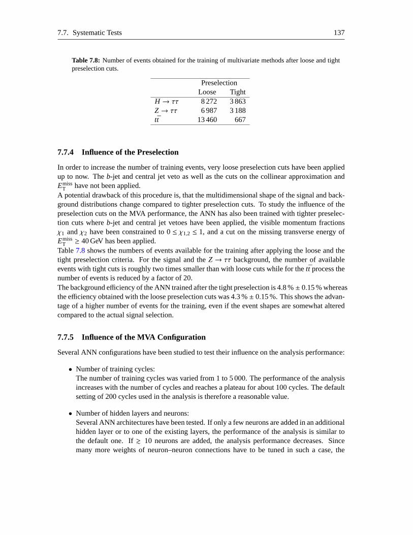
7.7. Systematic Tests 137
Table 7.8: Number of events obtained for the training of multivariate methods after loose and tightpreselection cuts.
PreselectionLoose Tight
H → ττ 8 272 3 863Z→ ττ 6 987 3 188tt 13 460 667
7.7.4 Influence of the Preselection
In order to increase the number of training events, very loose preselection cuts have been appliedup to now. Theb-jet and central jet veto as well as the cuts on the collinear approximation andEmiss
T have not been applied.A potential drawback of this procedure is, that the multidimensional shape ofthe signal and back-ground distributions change compared to tighter preselection cuts. To studythe influence of thepreselection cuts on the MVA performance, the ANN has also been trained with tighter preselec-tion cuts whereb-jet and central jet vetoes have been applied, the visible momentum fractionsχ1 andχ2 have been constrained to 0≤ χ1,2 ≤ 1, and a cut on the missing transverse energy ofEmiss
T ≥ 40 GeV has been applied.Table7.8 shows the numbers of events available for the training after applying the loose and thetight preselection criteria. For the signal and theZ→ ττ background, the number of availableevents with tight cuts is roughly two times smaller than with loose cuts while for thett process thenumber of events is reduced by a factor of 20.The background efficiency of the ANN trained after the tight preselection is 4.8 %± 0.15 % whereasthe efficiency obtained with the loose preselection cuts was 4.3 %± 0.15 %. This shows the advan-tage of a higher number of events for the training, even if the event shapes are somewhat alteredcompared to the actual signal selection.
7.7.5 Influence of the MVA Configuration
Several ANN configurations have been studied to test their influence on the analysis performance:
• Number of training cycles:The number of training cycles was varied from 1 to 5 000. The performanceof the analysisincreases with the number of cycles and reaches a plateau for about 100cycles. The defaultsetting of 200 cycles used in the analysis is therefore a reasonable value.
• Number of hidden layers and neurons:Several ANN architectures have been tested. If only a few neurons are added in an additionalhidden layer or to one of the existing layers, the performance of the analysis is similar tothe default one. If& 10 neurons are added, the analysis performance decreases. Sincemany more weights of neuron–neuron connections have to be tuned in sucha case, the

138 Chapter 7. Multivariate Analysis
performance decrease may be due to an insufficient number of training cycles and/or trainingevents.
On the other hand, removing neurons leads to a decreased performanceas well. With toofew neurons in the network, there are not enough degrees of freedom to describe the signaland background shapes in the multidimensional space.
The default setting of two hidden layers withN + 1 andN neurons, whereN is the numberof input variables, is best suited for this analysis.
• Learning rate:The learning rateη was increased and decreased by factors of 5. While the ANN trainedwith the lower learning rate shows a selection efficiency comparable to the default setup, thehigher learning rate results in a degraded performance. Again, the default setting of 0.02 forthe learning rate is optimal for this analysis.
7.7.6 Influence on themττ Distribution
Since the signal significance depends on themττ spectrum after applying all analysis cuts, it isimportant that the signal selection criteria do not influence themττ distributions of signal andbackground. Figure7.13 shows the shape for the signal as well as for theZ→ ττ and thettbackground separately for signal-like events (high ANN output values)and background-like events(low output values).No significant differences in the mass shapes are observed as expected, since the set ofinputvariables has been selected in order to minimize the bias of themττ distribution (see Section7.4).
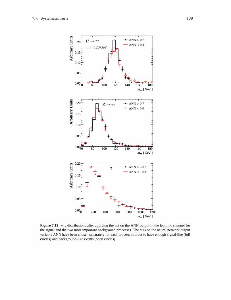
7.7. Systematic Tests 139
6060 8080 100100 120120 140140 160160 1801800.000.00
0.050.05
0.100.10
0.150.15
0.200.20
Arb
itrar
yU
nits
Arb
itrar
yU
nits
mττ [ GeV ]mττ [ GeV ]
ANN < 0.4
ANN > 0.7H → ττmH =120 GeV
6060 8080 100100 120120 140140 160160 1801800.000.00
0.050.05
0.100.10
0.150.15
0.200.20
Arb
itrar
yU
nits
Arb
itrar
yU
nits
mττ [ GeV ]mττ [ GeV ]
ANN > 0.7
ANN < 0.0Z→ ττ
00 200200 400400 600600 800800 10001000 120012000.000.00
0.050.05
0.100.10
0.150.15
0.200.20
Arb
itrar
yU
nits
Arb
itrar
yU
nits
mττ [ GeV ]mττ [ GeV ]
ANN > −0.7
ANN < −0.8tt
Figure 7.13: mττ distributions after applying the cut on the ANN output in theleptonic channel forthe signal and the two most important background processes.The cuts on the neural network outputvariable ANN have been chosen separately for each process inorder to have enough signal-like (fullcircles) and background-like events (open circles).

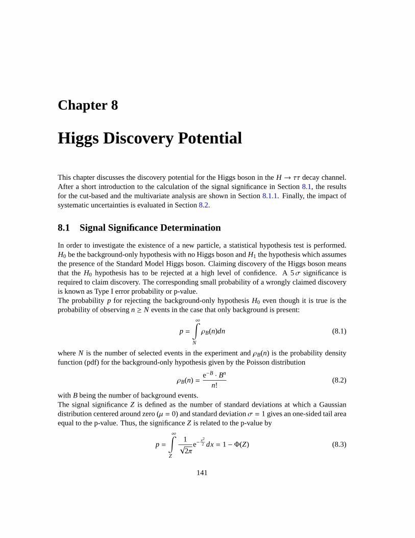
Chapter 8
Higgs Discovery Potential
This chapter discusses the discovery potential for the Higgs boson in theH → ττ decay channel.After a short introduction to the calculation of the signal significance in Section 8.1, the resultsfor the cut-based and the multivariate analysis are shown in Section8.1.1. Finally, the impact ofsystematic uncertainties is evaluated in Section8.2.
8.1 Signal Significance Determination
In order to investigate the existence of a new particle, a statistical hypothesis test is performed.H0 be the background-only hypothesis with no Higgs boson andH1 the hypothesis which assumesthe presence of the Standard Model Higgs boson. Claiming discovery of the Higgs boson meansthat theH0 hypothesis has to be rejected at a high level of confidence. A 5σ significance isrequired to claim discovery. The corresponding small probability of a wrongly claimed discoveryis known as Type I error probability or p-value.The probabilityp for rejecting the background-only hypothesisH0 even though it is true is theprobability of observingn ≥ N events in the case that only background is present:
p =
∞∫
N
ρB(n)dn (8.1)
whereN is the number of selected events in the experiment andρB(n) is the probability densityfunction (pdf) for the background-only hypothesis given by the Poisson distribution
ρB(n) =e−B · Bn
n!(8.2)
with B being the number of background events.The signal significanceZ is defined as the number of standard deviations at which a Gaussiandistribution centered around zero (µ = 0) and standard deviationσ = 1 gives an one-sided tail areaequal to the p-value. Thus, the significanceZ is related to the p-value by
p =
∞∫
Z
1√
2πe−
x22 dx= 1− Φ(Z) (8.3)
141
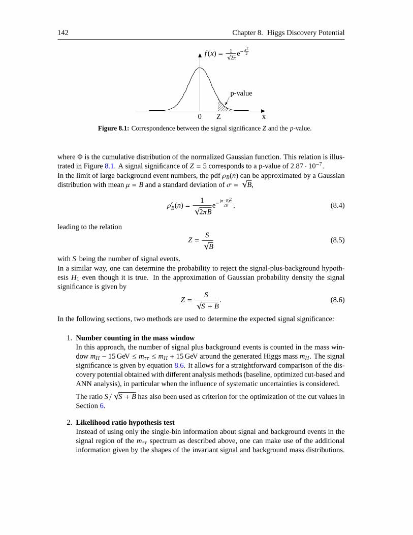
142 Chapter 8. Higgs Discovery Potential
Z0 x
p-value
f (x) = 1√2π
e−x22
Figure 8.1: Correspondence between the signal significanceZ and thep-value.
whereΦ is the cumulative distribution of the normalized Gaussian function. This relation isillus-trated in Figure8.1. A signal significance ofZ = 5 corresponds to a p-value of 2.87 · 10−7.In the limit of large background event numbers, the pdfρB(n) can be approximated by a Gaussiandistribution with meanµ = B and a standard deviation ofσ =
√B,
ρ′B(n) =1√
2πBe−
(n−B)2
2B , (8.4)
leading to the relation
Z =S√
B(8.5)
with S being the number of signal events.In a similar way, one can determine the probability to reject the signal-plus-background hypoth-esisH1 even though it is true. In the approximation of Gaussian probability density thesignalsignificance is given by
Z =S
√S + B
. (8.6)
In the following sections, two methods are used to determine the expected signal significance:
1. Number counting in the mass windowIn this approach, the number of signal plus background events is counted in the mass win-dow mH − 15 GeV≤ mττ ≤ mH + 15 GeV around the generated Higgs massmH. The signalsignificance is given by equation8.6. It allows for a straightforward comparison of the dis-covery potential obtained with different analysis methods (baseline, optimized cut-based andANN analysis), in particular when the influence of systematic uncertainties is considered.
The ratioS/√
S + B has also been used as criterion for the optimization of the cut values inSection6.
2. Likelihood ratio hypothesis testInstead of using only the single-bin information about signal and background events in thesignal region of themττ spectrum as described above, one can make use of the additionalinformation given by the shapes of the invariant signal and backgroundmass distributions.
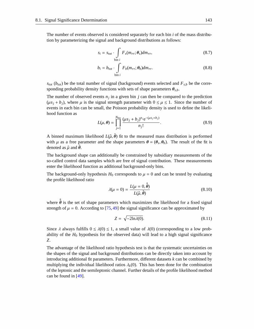
8.1. Signal Significance Determination 143
The number of events observed is considered separately for each bini of the mass distribu-tion by parameterizing the signal and background distributions as follows:
si = stot ·∫
bin i
Fs(mττ; θs)dmττ, (8.7)
bi = btot ·∫
bin i
Fb(mττ; θb)dmττ. (8.8)
stot (btot) be the total number of signal (background) events selected andFs,b be the corre-sponding probability density functions with sets of shape parametersθs,b.
The number of observed eventsn j in a given bin j can then be compared to the prediction(µsj + b j), whereµ is the signal strength parameter with 0≤ µ ≤ 1. Since the number ofevents in each bin can be small, the Poisson probability density is used to definethe likeli-hood function as
L(µ, θ) =Nbin∏
j=1
(µsj + b j)n j e−(µsj+b j )
n j !. (8.9)
A binned maximum likelihoodL(µ, θ) fit to the measured mass distribution is performedwith µ as a free parameter and the shape parametersθ = (θs, θb). The result of the fit isdenoted as ˆµ andθ.
The background shape can additionally be constrained by subsidiary measurements of theso-called control data samples which are free of signal contribution. These measurementsenter the likelihood function as additional background-only bins.
The background-only hypothesisH0 corresponds toµ = 0 and can be tested by evaluatingthe profile likelihood ratio
λ(µ = 0) =L(µ = 0, ˆθ)
L(µ, θ)(8.10)
where ˆθ is the set of shape parameters which maximizes the likelihood for a fixed signalstrength ofµ = 0. According to [75,49] the signal significance can be approximated by
Z =√
−2lnλ(0). (8.11)
Sinceλ always fulfills 0≤ λ(0) ≤ 1, a small value ofλ(0) (corresponding to a low prob-ability of the H0 hypothesis for the observed data) will lead to a high signal significanceZ.
The advantage of the likelihood ratio hypothesis test is that the systematic uncertainties onthe shapes of the signal and background distributions can be directly taken into account byintroducing additional fit parameters. Furthermore, different datasetsk can be combined bymultiplying the individual likelihood ratiosλk(0). This has been done for the combinationof the leptonic and the semileptonic channel. Further details of the profile likelihood methodcan be found in [49].
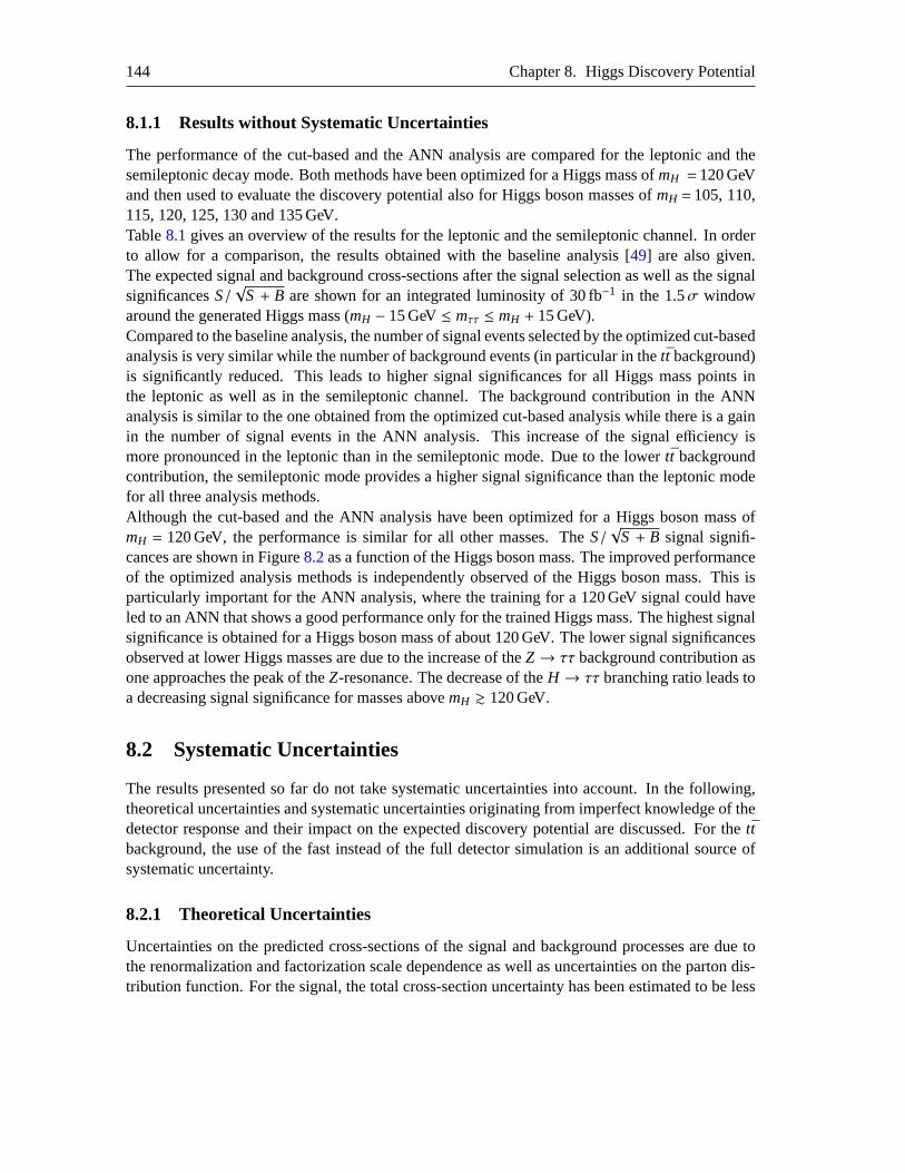
144 Chapter 8. Higgs Discovery Potential
8.1.1 Results without Systematic Uncertainties
The performance of the cut-based and the ANN analysis are compared for the leptonic and thesemileptonic decay mode. Both methods have been optimized for a Higgs mass ofmH =120 GeVand then used to evaluate the discovery potential also for Higgs boson masses ofmH =105, 110,115, 120, 125, 130 and 135 GeV.Table8.1gives an overview of the results for the leptonic and the semileptonic channel. In orderto allow for a comparison, the results obtained with the baseline analysis [49] are also given.The expected signal and background cross-sections after the signalselection as well as the signalsignificancesS/
√S + B are shown for an integrated luminosity of 30 fb−1 in the 1.5σ window
around the generated Higgs mass (mH − 15 GeV≤ mττ ≤ mH + 15 GeV).Compared to the baseline analysis, the number of signal events selected by the optimized cut-basedanalysis is very similar while the number of background events (in particular inthett background)is significantly reduced. This leads to higher signal significances for all Higgs mass points inthe leptonic as well as in the semileptonic channel. The background contribution in the ANNanalysis is similar to the one obtained from the optimized cut-based analysis while there is a gainin the number of signal events in the ANN analysis. This increase of the signal efficiency ismore pronounced in the leptonic than in the semileptonic mode. Due to the lowertt backgroundcontribution, the semileptonic mode provides a higher signal significance thanthe leptonic modefor all three analysis methods.Although the cut-based and the ANN analysis have been optimized for a Higgsboson mass ofmH = 120 GeV, the performance is similar for all other masses. TheS/
√S + B signal signifi-
cances are shown in Figure8.2as a function of the Higgs boson mass. The improved performanceof the optimized analysis methods is independently observed of the Higgs bosonmass. This isparticularly important for the ANN analysis, where the training for a 120 GeVsignal could haveled to an ANN that shows a good performance only for the trained Higgs mass. The highest signalsignificance is obtained for a Higgs boson mass of about 120 GeV. The lower signal significancesobserved at lower Higgs masses are due to the increase of theZ→ ττ background contribution asone approaches the peak of theZ-resonance. The decrease of theH → ττ branching ratio leads toa decreasing signal significance for masses abovemH & 120 GeV.
8.2 Systematic Uncertainties
The results presented so far do not take systematic uncertainties into account. In the following,theoretical uncertainties and systematic uncertainties originating from imperfect knowledge of thedetector response and their impact on the expected discovery potential are discussed. For thettbackground, the use of the fast instead of the full detector simulation is an additional source ofsystematic uncertainty.
8.2.1 Theoretical Uncertainties
Uncertainties on the predicted cross-sections of the signal and background processes are due tothe renormalization and factorization scale dependence as well as uncertainties on the parton dis-tribution function. For the signal, the total cross-section uncertainty has been estimated to be less
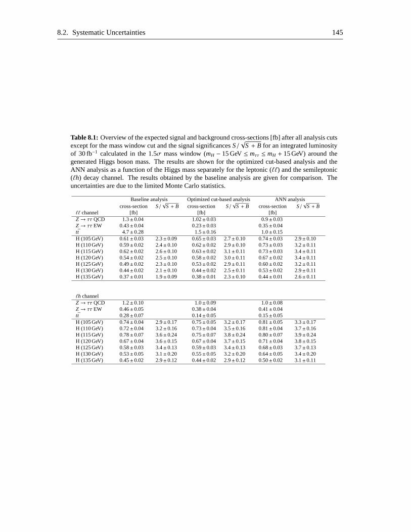
8.2. Systematic Uncertainties 145
Table 8.1: Overview of the expected signal and background cross-sections [fb] after all analysis cutsexcept for the mass window cut and the signal significancesS/
√S + B for an integrated luminosity
of 30 fb−1 calculated in the 1.5σ mass window (mH − 15 GeV≤ mττ ≤ mH + 15 GeV) around thegenerated Higgs boson mass. The results are shown for the optimized cut-based analysis and theANN analysis as a function of the Higgs mass separately for the leptonic (ℓℓ) and the semileptonic(ℓh) decay channel. The results obtained by the baseline analysis are given for comparison. Theuncertainties are due to the limited Monte Carlo statistics.
Baseline analysis Optimized cut-based analysis ANN analysiscross-section S/
√S + B cross-section S/
√S + B cross-section S/
√S + B
ℓℓ channel [fb] [fb] [fb]Z→ ττ QCD 1.3± 0.04 1.02±0.03 0.9± 0.03Z→ ττ EW 0.43± 0.04 0.23±0.03 0.35± 0.04tt 4.7± 0.28 1.5±0.16 1.0± 0.15H (105 GeV) 0.61± 0.03 2.3± 0.09 0.65±0.03 2.7± 0.10 0.74± 0.03 2.9± 0.10H (110 GeV) 0.59± 0.02 2.4± 0.10 0.62±0.02 2.9± 0.10 0.73± 0.03 3.2± 0.11H (115 GeV) 0.62± 0.02 2.6± 0.10 0.63±0.02 3.1± 0.11 0.73± 0.03 3.4± 0.11H (120 GeV) 0.54± 0.02 2.5± 0.10 0.58±0.02 3.0± 0.11 0.67± 0.02 3.4± 0.11H (125 GeV) 0.49± 0.02 2.3± 0.10 0.53±0.02 2.9± 0.11 0.60± 0.02 3.2± 0.11H (130 GeV) 0.44± 0.02 2.1± 0.10 0.44±0.02 2.5± 0.11 0.53± 0.02 2.9± 0.11H (135 GeV) 0.37± 0.01 1.9± 0.09 0.38±0.01 2.3± 0.10 0.44± 0.01 2.6± 0.11
ℓh channelZ→ ττ QCD 1.2± 0.10 1.0±0.09 1.0± 0.08Z→ ττ EW 0.46± 0.05 0.38±0.04 0.41± 0.04tt 0.28± 0.07 0.14±0.05 0.15± 0.05H (105 GeV) 0.74± 0.04 2.9± 0.17 0.75±0.05 3.2± 0.17 0.81± 0.05 3.3± 0.17H (110 GeV) 0.72± 0.04 3.2± 0.16 0.73±0.04 3.5± 0.16 0.81± 0.04 3.7± 0.16H (115 GeV) 0.78± 0.07 3.6± 0.24 0.75±0.07 3.8± 0.24 0.80± 0.07 3.9± 0.24H (120 GeV) 0.67± 0.04 3.6± 0.15 0.67±0.04 3.7± 0.15 0.71± 0.04 3.8± 0.15H (125 GeV) 0.58± 0.03 3.4± 0.13 0.59±0.03 3.4± 0.13 0.68± 0.03 3.7± 0.13H (130 GeV) 0.53± 0.05 3.1± 0.20 0.55±0.05 3.2± 0.20 0.64± 0.05 3.4± 0.20H (135 GeV) 0.45± 0.02 2.9± 0.12 0.44±0.02 2.9± 0.12 0.50± 0.02 3.1± 0.11
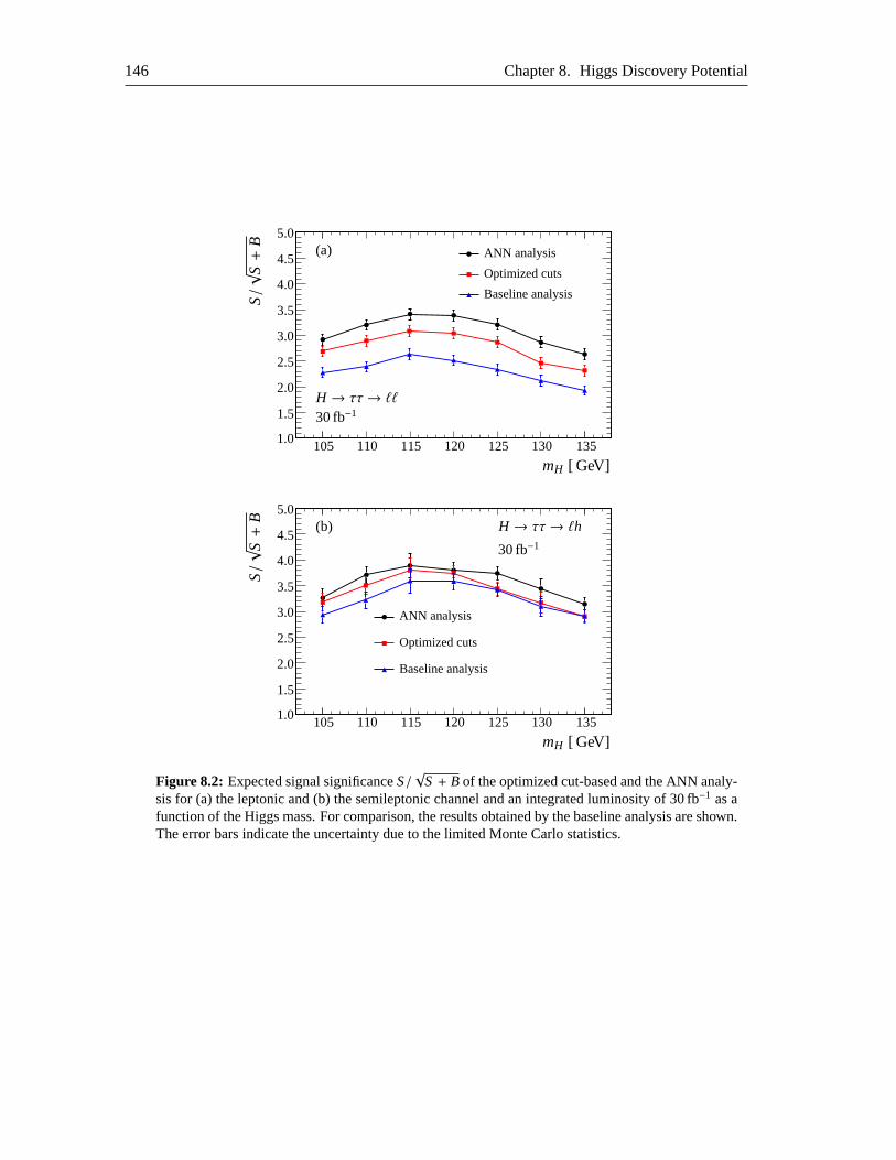
146 Chapter 8. Higgs Discovery Potential
105 110 115 120 125 130 1351.0
1.5
2.0
2.5
3.0
3.5
4.0
4.5
5.0
S/√
S+
B
mH [ GeV]
ANN analysis
Optimized cuts
Baseline analysis
(a)
H → ττ→ ℓℓ30 fb−1
105 110 115 120 125 130 1351.0
1.5
2.0
2.5
3.0
3.5
4.0
4.5
5.0
S/√
S+
B
mH [ GeV]
ANN analysis
Optimized cuts
Baseline analysis
(b) H → ττ→ ℓh30 fb−1
Figure 8.2: Expected signal significanceS/√
S + B of the optimized cut-based and the ANN analy-sis for (a) the leptonic and (b) the semileptonic channel andan integrated luminosity of 30 fb−1 as afunction of the Higgs mass. For comparison, the results obtained by the baseline analysis are shown.The error bars indicate the uncertainty due to the limited Monte Carlo statistics.
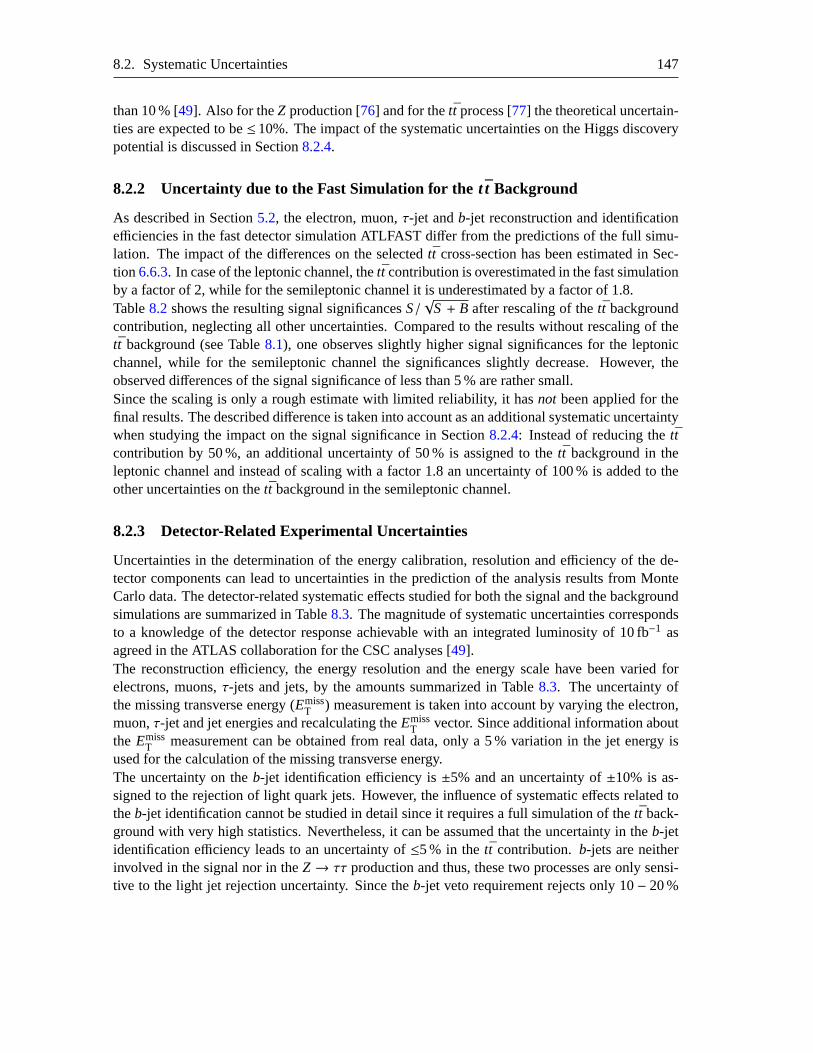
8.2. Systematic Uncertainties 147
than 10 % [49]. Also for theZ production [76] and for thett process [77] the theoretical uncertain-ties are expected to be≤10%. The impact of the systematic uncertainties on the Higgs discoverypotential is discussed in Section8.2.4.
8.2.2 Uncertainty due to the Fast Simulation for thet t Background
As described in Section5.2, the electron, muon,τ-jet andb-jet reconstruction and identificationefficiencies in the fast detector simulation ATLFAST differ from the predictions of the full simu-lation. The impact of the differences on the selectedtt cross-section has been estimated in Sec-tion 6.6.3. In case of the leptonic channel, thett contribution is overestimated in the fast simulationby a factor of 2, while for the semileptonic channel it is underestimated by a factor of 1.8.Table8.2 shows the resulting signal significancesS/
√S + B after rescaling of thett background
contribution, neglecting all other uncertainties. Compared to the results without rescaling of thett background (see Table8.1), one observes slightly higher signal significances for the leptonicchannel, while for the semileptonic channel the significances slightly decrease. However, theobserved differences of the signal significance of less than 5 % are rather small.Since the scaling is only a rough estimate with limited reliability, it hasnot been applied for thefinal results. The described difference is taken into account as an additional systematic uncertaintywhen studying the impact on the signal significance in Section8.2.4: Instead of reducing thettcontribution by 50 %, an additional uncertainty of 50 % is assigned to thett background in theleptonic channel and instead of scaling with a factor 1.8 an uncertainty of 100 % is added to theother uncertainties on thett background in the semileptonic channel.
8.2.3 Detector-Related Experimental Uncertainties
Uncertainties in the determination of the energy calibration, resolution and efficiency of the de-tector components can lead to uncertainties in the prediction of the analysis results from MonteCarlo data. The detector-related systematic effects studied for both the signal and the backgroundsimulations are summarized in Table8.3. The magnitude of systematic uncertainties correspondsto a knowledge of the detector response achievable with an integrated luminosity of 10 fb−1 asagreed in the ATLAS collaboration for the CSC analyses [49].The reconstruction efficiency, the energy resolution and the energy scale have been varied forelectrons, muons,τ-jets and jets, by the amounts summarized in Table8.3. The uncertainty ofthe missing transverse energy (Emiss
T ) measurement is taken into account by varying the electron,muon,τ-jet and jet energies and recalculating theEmiss
T vector. Since additional information aboutthe Emiss
T measurement can be obtained from real data, only a 5 % variation in the jet energy isused for the calculation of the missing transverse energy.The uncertainty on theb-jet identification efficiency is±5% and an uncertainty of±10% is as-signed to the rejection of light quark jets. However, the influence of systematic effects related totheb-jet identification cannot be studied in detail since it requires a full simulation of the tt back-ground with very high statistics. Nevertheless, it can be assumed that the uncertainty in theb-jetidentification efficiency leads to an uncertainty of≤5 % in thett contribution. b-jets are neitherinvolved in the signal nor in theZ→ ττ production and thus, these two processes are only sensi-tive to the light jet rejection uncertainty. Since theb-jet veto requirement rejects only 10− 20 %
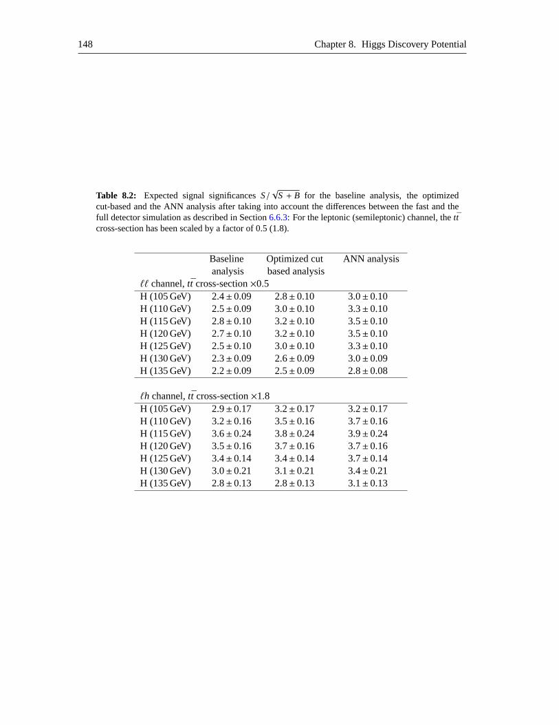
148 Chapter 8. Higgs Discovery Potential
Table 8.2: Expected signal significancesS/√
S + B for the baseline analysis, the optimizedcut-based and the ANN analysis after taking into account thedifferences between the fast and thefull detector simulation as described in Section6.6.3: For the leptonic (semileptonic) channel, thettcross-section has been scaled by a factor of 0.5 (1.8).
Baseline Optimized cut ANN analysisanalysis based analysis
ℓℓ channel,tt cross-section×0.5H (105 GeV) 2.4±0.09 2.8±0.10 3.0±0.10H (110 GeV) 2.5±0.09 3.0±0.10 3.3±0.10H (115 GeV) 2.8±0.10 3.2±0.10 3.5±0.10H (120 GeV) 2.7±0.10 3.2±0.10 3.5±0.10H (125 GeV) 2.5±0.10 3.0±0.10 3.3±0.10H (130 GeV) 2.3±0.09 2.6±0.09 3.0±0.09H (135 GeV) 2.2±0.09 2.5±0.09 2.8±0.08
ℓh channel,tt cross-section×1.8H (105 GeV) 2.9±0.17 3.2±0.17 3.2±0.17H (110 GeV) 3.2±0.16 3.5±0.16 3.7±0.16H (115 GeV) 3.6±0.24 3.8±0.24 3.9±0.24H (120 GeV) 3.5±0.16 3.7±0.16 3.7±0.16H (125 GeV) 3.4±0.14 3.4±0.14 3.7±0.14H (130 GeV) 3.0±0.21 3.1±0.21 3.4±0.21H (135 GeV) 2.8±0.13 2.8±0.13 3.1±0.13
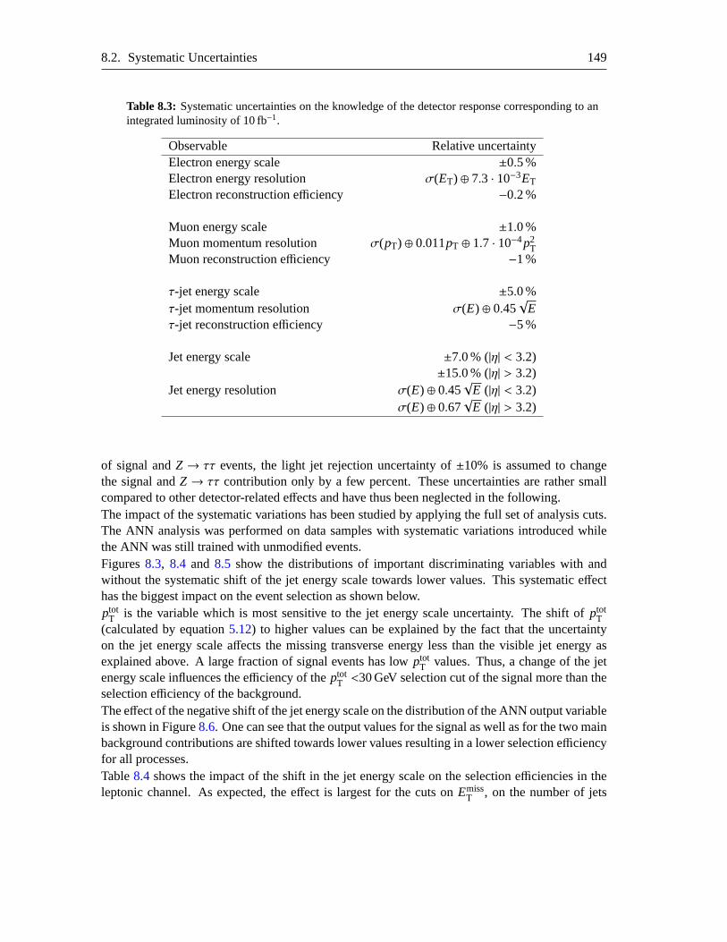
8.2. Systematic Uncertainties 149
Table 8.3: Systematic uncertainties on the knowledge of the detector response corresponding to anintegrated luminosity of 10 fb−1.
Observable Relative uncertaintyElectron energy scale ±0.5 %Electron energy resolution σ(ET) ⊕ 7.3 · 10−3ET
Electron reconstruction efficiency −0.2 %
Muon energy scale ±1.0 %Muon momentum resolution σ(pT) ⊕ 0.011pT ⊕ 1.7 · 10−4p2
TMuon reconstruction efficiency −1 %
τ-jet energy scale ±5.0 %τ-jet momentum resolution σ(E) ⊕ 0.45
√E
τ-jet reconstruction efficiency −5 %
Jet energy scale ±7.0 % (|η| < 3.2)±15.0 % (|η| > 3.2)
Jet energy resolution σ(E) ⊕ 0.45√
E (|η| < 3.2)σ(E) ⊕ 0.67
√E (|η| > 3.2)
of signal andZ→ ττ events, the light jet rejection uncertainty of±10% is assumed to changethe signal andZ→ ττ contribution only by a few percent. These uncertainties are rather smallcompared to other detector-related effects and have thus been neglected in the following.The impact of the systematic variations has been studied by applying the full set of analysis cuts.The ANN analysis was performed on data samples with systematic variations introduced whilethe ANN was still trained with unmodified events.Figures8.3, 8.4 and 8.5 show the distributions of important discriminating variables with andwithout the systematic shift of the jet energy scale towards lower values. This systematic effecthas the biggest impact on the event selection as shown below.ptot
T is the variable which is most sensitive to the jet energy scale uncertainty. Theshift of ptotT
(calculated by equation5.12) to higher values can be explained by the fact that the uncertaintyon the jet energy scale affects the missing transverse energy less than the visible jet energy asexplained above. A large fraction of signal events has lowptot
T values. Thus, a change of the jetenergy scale influences the efficiency of theptot
T <30 GeV selection cut of the signal more than theselection efficiency of the background.The effect of the negative shift of the jet energy scale on the distribution of the ANN output variableis shown in Figure8.6. One can see that the output values for the signal as well as for the two mainbackground contributions are shifted towards lower values resulting in a lower selection efficiencyfor all processes.Table8.4 shows the impact of the shift in the jet energy scale on the selection efficiencies in theleptonic channel. As expected, the effect is largest for the cuts onEmiss
T , on the number of jets
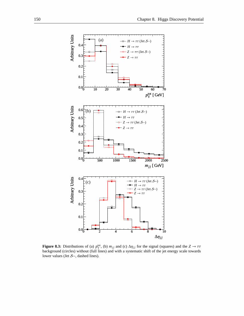
150 Chapter 8. Higgs Discovery Potential
00 1010 2020 3030 4040 5050 6060 70700.00.0
0.10.1
0.20.2
0.30.3
0.40.4
Arb
itrar
yU
nits
Arb
itrar
yU
nits
ptotT [ GeV]ptotT [ GeV]
H → ττH → ττ (JetS−)
Z→ ττZ→ ττ (JetS−)
(a)
00 500500 10001000 15001500 20002000 250025000.00.0
0.10.1
0.20.2
0.30.3
0.40.4
0.50.5
0.60.6
Arb
itrar
yU
nits
Arb
itrar
yU
nits
mj j [ GeV]mj j [ GeV]
H → ττH → ττ (JetS−)
Z→ ττZ→ ττ (JetS−)
(b)
00 22 44 66 88 10100.00.0
0.10.1
0.20.2
0.30.3
0.40.4
Arb
itrar
yU
nits
Arb
itrar
yU
nits
∆η j j∆η j j
H → ττH → ττ (JetS−)
Z→ ττZ→ ττ (JetS−)
(c)
Figure 8.3: Distributions of (a)ptotT , (b) mj j and (c)∆η j j for the signal (squares) and theZ→ ττ
background (circles) without (full lines) and with a systematic shift of the jet energy scale towardslower values (JetS−, dashed lines).
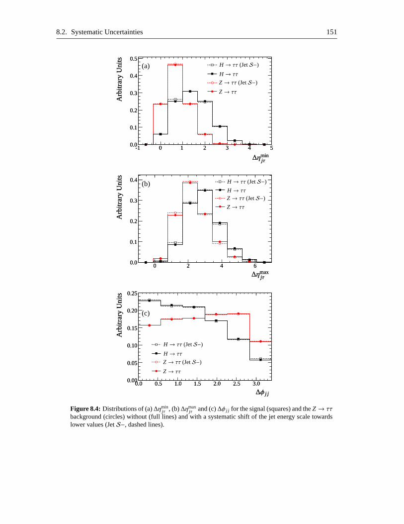
8.2. Systematic Uncertainties 151
-1-1 00 11 22 33 44 550.00.0
0.10.1
0.20.2
0.30.3
0.40.4
0.50.5
Arb
itrar
yU
nits
Arb
itrar
yU
nits
∆ηminjτ∆ηminjτ
H → ττH → ττ (JetS−)
Z→ ττZ→ ττ (JetS−)
(a)
00 22 44 660.00.0
0.10.1
0.20.2
0.30.3
0.40.4
Arb
itrar
yU
nits
Arb
itrar
yU
nits
∆ηmaxjτ∆ηmaxjτ
H → ττH → ττ (JetS−)
Z→ ττZ→ ττ (JetS−)
(b)
0.00.0 0.50.5 1.01.0 1.51.5 2.02.0 2.52.5 3.03.00.000.00
0.050.05
0.100.10
0.150.15
0.200.20
0.250.25
Arb
itrar
yU
nits
Arb
itrar
yU
nits
∆φ j j∆φ j j
H → ττH → ττ (JetS−)
Z→ ττZ→ ττ (JetS−)
(c)
Figure 8.4: Distributions of (a)∆ηminjτ , (b)∆ηmax
jτ and (c)∆φ j j for the signal (squares) and theZ→ ττbackground (circles) without (full lines) and with a systematic shift of the jet energy scale towardslower values (JetS−, dashed lines).
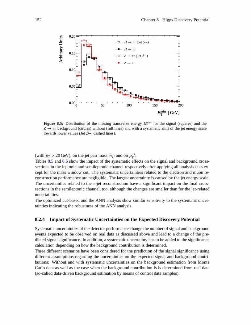
152 Chapter 8. Higgs Discovery Potential
00 5050 100100 150150 2002000.000.00
0.050.05
0.100.10
0.150.15
0.200.20
Arb
itrar
yU
nits
Arb
itrar
yU
nits
EmissT [ GeV]EmissT [ GeV]
H → ττ
H → ττ (JetS−)
Z→ ττ
Z→ ττ (JetS−)
Figure 8.5: Distribution of the missing transverse energyEmissT for the signal (squares) and the
Z→ ττ background (circles) without (full lines) and with a systematic shift of the jet energy scaletowards lower values (JetS−, dashed lines).
(with pT > 20 GeV), on the jet pair massmj j and onptotT .
Tables8.5and8.6show the impact of the systematic effects on the signal and background cross-sections in the leptonic and semileptonic channel respectively after applyingall analysis cuts ex-cept for the mass window cut. The systematic uncertainties related to the electron and muon re-construction performance are negligible. The largest uncertainty is caused by the jet energy scale.The uncertainties related to theτ-jet reconstruction have a significant impact on the final cross-sections in the semileptonic channel, too, although the changes are smaller thanfor the jet-relateduncertainties.The optimized cut-based and the ANN analysis show similar sensitivity to the systematic uncer-tainties indicating the robustness of the ANN analysis.
8.2.4 Impact of Systematic Uncertainties on the Expected Discovery Potential
Systematic uncertainties of the detector performance change the number of signal and backgroundevents expected to be observed on real data as discussed above and lead to a change of the pre-dicted signal significance. In addition, a systematic uncertainty has to be added to the significancecalculation depending on how the background contribution is determined.Three different scenarios have been considered for the prediction of the signalsignificance usingdifferent assumptions regarding the uncertainties on the expected signal andbackground contri-butions: Without and with systematic uncertainties on the background estimation from MonteCarlo data as well as the case when the background contribution is is determined from real data(so-called data-driven background estimation by means of control data samples).
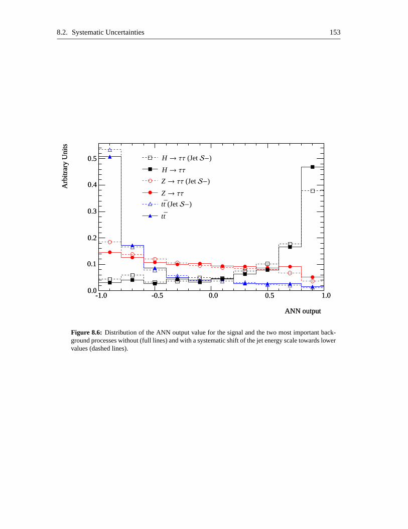
8.2. Systematic Uncertainties 153
-1.0-1.0 -0.5-0.50.0
0.00.0
0.0
0.10.1
0.20.2
0.30.3
0.40.4
0.5
0.5
0.5
0.5 1.01.0
0.40
Arb
itrar
yU
nits
Arb
itrar
yU
nits
H → ττH → ττ (JetS−)
Z→ ττZ→ ττ (JetS−)
tt
tt (JetS−)
ANN outputANN output
Figure 8.6: Distribution of the ANN output value for the signal and the two most important back-ground processes without (full lines) and with a systematicshift of the jet energy scale towards lowervalues (dashed lines).

154 Chapter 8. Higgs Discovery Potential
Table 8.4: Comparison of the cut efficiencies [%] with and without a shift of the jet energy scaletowards lower values (JetS−) for the signal and theZ→ ττ and tt backgrounds in the leptonicchannel. The discriminating variables which are affected the most are indicated by the shaded lines.
H → ττ Z→ ττ + jets ttJetS− applied? No Yes No Yes No YesTrigger 53 53 49 49 29 29N(e+ µ)=2 47 47 58 58 13 13Lepton charge 100 100 100 100 98 98Emiss
T > 40 GeV 58 55 45 42 78 77∆φττ < 2.5 90 91 94 94 70 70χ1,2 = 0.0− 1.0 90 89 85 84 16 15mℓνT < 100 GeV 100 100 100 100 82 84N(jets)≥ 2 82 79 89 85 95 92η j1 × η j2 < 0 83 84 62 62 47 46∆η jτ > 0 91 91 57 56 38 38∆η j j > 3.5 83 83 50 48 34 34mj j > 600 GeV 82 79 44 38 68 65∆φ j j < 2.2 82 82 65 64 70 70b-jet veto 89 90 87 86 76 78∆ηmin
jτ > 0.6 93 93 70 71 74 75∆ηmax
jτ > 1.5 99 100 100 100 95 94Central jet veto 85 87 86 89 9 10ptot
T < 30 GeV 93 88 90 85 52 40
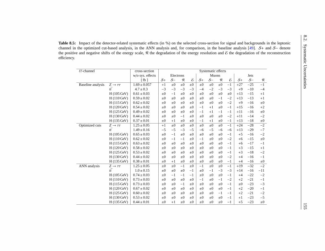
8.2.S
ystematic
Uncertainties
155
Table 8.5: Impact of the detector-related systematic effects (in %) on the selected cross-section for signal and backgrounds in the leptonicchannel in the optimized cut-based analysis, in the ANN analysis and, for comparison, in the baseline analysis [49]. S+ andS− denotethe positive and negative shifts of the energy scale,R the degradation of the energy resolution andE the degradation of the reconstructionefficiency.
ℓℓ-channel cross-section Systematic effectsw/o sys. effects Electrons Muons Jets
[ fb ] S+ S− R E S+ S− R E S+ S− RBaseline analysis Z→ ττ 1.69±0.057 +1 ±0 ±0 ±0 ±0 ±0 ±0 −1 +27 −25 −1
tt 4.7±0.3 −3 −3 −3 −3 −4 −2 −3 −3 +9 −10 −4H (105 GeV) 0.61±0.03 ±0 −1 ±0 ±0 ±0 ±0 ±0 ±0 +13 −15 +1H (110 GeV) 0.59±0.02 ±0 ±0 ±0 ±0 ±0 ±0 −1 −2 +13 −13 +1H (115 GeV) 0.62±0.02 ±0 ±0 ±0 ±0 ±0 ±0 ±0 −2 +9 −16 ±0H (120 GeV) 0.54±0.02 ±0 ±0 ±0 ±0 −1 +1 ±0 −1 +15 −16 +2H (125 GeV) 0.49±0.02 ±0 ±0 ±0 ±0 −1 +1 −1 −1 +11 −16 ±0H (130 GeV) 0.44±0.02 ±0 ±0 −1 ±0 ±0 ±0 ±0 −2 +11 −14 −2H (135 GeV) 0.37±0.01 ±0 +1 ±0 ±0 −1 +1 ±0 −1 +13 −18 ±0
Optimized cuts Z→ ττ 1.25±0.05 +1 ±0 ±0 ±0 ±0 ±0 ±0 −1 +24 −28 −2tt 1.49±0.16 −5 −5 −3 −5 −6 −5 −6 −6 +13 −29 −7H (105 GeV) 0.65±0.03 ±0 −1 ±0 ±0 ±0 ±0 ±0 −1 +5 −16 −2H (110 GeV) 0.62±0.02 ±0 −1 −1 ±0 −1 ±0 ±0 −2 +6 −15 ±0H (115 GeV) 0.63±0.02 ±0 ±0 ±0 ±0 ±0 ±0 ±0 −1 +6 −17 −1H (120 GeV) 0.58±0.02 ±0 ±0 ±0 ±0 ±0 ±0 ±0 −1 +3 −15 +1H (125 GeV) 0.53±0.02 ±0 ±0 ±0 ±0 ±0 ±0 ±0 −1 +3 −18 −2H (130 GeV) 0.44±0.02 ±0 ±0 ±0 ±0 ±0 ±0 ±0 −2 +4 −16 −1H (135 GeV) 0.38±0.01 ±0 +1 ±0 ±0 ±0 ±0 ±0 −1 +4 −16 ±0
ANN analysis Z→ ττ 1.25±0.05 ±0 ±0 −1 ±0 −1 ±0 ±0 −1 +19 −32 −2tt 1.0±0.15 ±0 ±0 ±0 −1 ±0 −1 −3 −3 +14 −16 −11H (105 GeV) 0.74±0.03 ±0 −1 −1 −1 ±0 ±0 ±0 −1 +4 −22 −2H (110 GeV) 0.73±0.03 ±0 ±0 ±0 ±0 −1 ±0 −1 −2 +2 −21 −1H (115 GeV) 0.73±0.03 ±0 ±0 −1 ±0 ±0 ±0 ±0 −1 ±0 −23 −3H (120 GeV) 0.67±0.02 ±0 ±0 ±0 ±0 ±0 ±0 ±0 −1 +2 −20 −1H (125 GeV) 0.60±0.02 ±0 ±0 ±0 ±0 ±0 ±0 −1 −1 +2 −21 −2H (130 GeV) 0.53±0.02 ±0 ±0 ±0 ±0 ±0 ±0 ±0 −1 +1 −23 −5H (135 GeV) 0.44±0.01 ±0 +1 ±0 ±0 ±0 ±0 ±0 −1 +5 −23 ±0
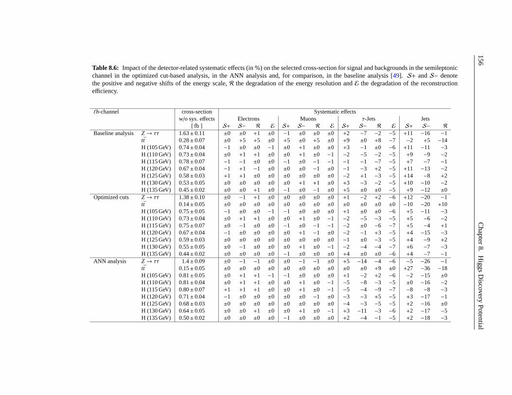
156C
hapter8.
Higgs
Discovery
Potential
Table 8.6: Impact of the detector-related systematic effects (in %) on the selected cross-section for signal and backgrounds in the semileptonicchannel in the optimized cut-based analysis, in the ANN analysis and, for comparison, in the baseline analysis [49]. S+ andS− denotethe positive and negative shifts of the energy scale,R the degradation of the energy resolution andE the degradation of the reconstructionefficiency.
ℓh-channel cross-section Systematic effectsw/o sys. effects Electrons Muons τ-Jets Jets
[ fb ] S+ S− R E S+ S− R E S+ S− R E S+ S− RBaseline analysis Z→ ττ 1.63±0.11 ±0 ±0 +1 ±0 −1 ±0 ±0 ±0 +2 −7 −2 −5 +11 −16 −1
tt 0.28±0.07 ±0 +5 +5 ±0 +5 ±0 +5 ±0 +9 ±0 +8 −7 −2 +5 −14H (105 GeV) 0.74±0.04 −1 ±0 ±0 −1 ±0 +1 ±0 ±0 +3 −1 ±0 −6 +11 −11 −3H (110 GeV) 0.73±0.04 ±0 +1 +1 ±0 ±0 +1 ±0 −1 −2 −5 −2 −5 +9 −9 −2H (115 GeV) 0.78±0.07 −1 −1 ±0 ±0 −1 ±0 −1 −1 −1 −1 −7 −5 +7 −7 −1H (120 GeV) 0.67±0.04 −1 +1 −1 ±0 ±0 ±0 −1 ±0 −1 −3 +2 −5 +11 −13 −2H (125 GeV) 0.58±0.03 +1 +1 ±0 ±0 ±0 ±0 ±0 ±0 −2 +1 −3 −5 +14 −8 +2H (130 GeV) 0.53±0.05 ±0 ±0 ±0 ±0 ±0 +1 +1 ±0 +3 −3 −2 −5 +10 −10 −2H (135 GeV) 0.45±0.02 ±0 ±0 +1 ±0 −1 ±0 −1 ±0 +5 ±0 ±0 −5 +9 −12 ±0
Optimized cuts Z→ ττ 1.38±0.10 ±0 −1 +1 ±0 ±0 ±0 ±0 ±0 +1 −2 +2 −6 +12 −20 −1tt 0.14±0.05 ±0 ±0 ±0 ±0 ±0 ±0 ±0 ±0 ±0 ±0 ±0 ±0 −10 −20 +10H (105 GeV) 0.75±0.05 −1 ±0 ±0 −1 −1 ±0 ±0 ±0 +1 ±0 ±0 −6 +5 −11 −3H (110 GeV) 0.73±0.04 ±0 +1 +1 ±0 ±0 +1 ±0 −1 −2 −5 −3 −5 +5 −6 −2H (115 GeV) 0.75±0.07 ±0 −1 ±0 ±0 −1 ±0 −1 −1 −2 ±0 −6 −7 +5 −4 +1H (120 GeV) 0.67±0.04 −1 ±0 ±0 ±0 ±0 +1 −1 ±0 −2 −1 +3 −5 +4 −15 −3H (125 GeV) 0.59±0.03 ±0 ±0 ±0 ±0 ±0 ±0 ±0 ±0 −1 ±0 −3 −5 +4 −9 +2H (130 GeV) 0.55±0.05 ±0 −1 ±0 ±0 ±0 +1 ±0 −1 −2 −4 −4 −7 +6 −7 −3H (135 GeV) 0.44±0.02 ±0 ±0 ±0 ±0 −1 ±0 ±0 ±0 +4 ±0 ±0 −6 +4 −7 −1
ANN analysis Z→ ττ 1.4±0.09 ±0 −1 −1 ±0 ±0 −1 −1 ±0 +5 −14 −4 −6 −5 −26 −1tt 0.15±0.05 ±0 ±0 ±0 ±0 ±0 ±0 ±0 ±0 ±0 ±0 +9 ±0 +27 −36 −18H (105 GeV) 0.81±0.05 ±0 +1 +1 −1 −1 ±0 ±0 ±0 +1 −2 +2 −6 −2 −15 ±0H (110 GeV) 0.81±0.04 ±0 +1 +1 ±0 ±0 +1 ±0 −1 −5 −8 −3 −5 ±0 −16 −2H (115 GeV) 0.80±0.07 +1 +1 +1 ±0 ±0 +1 ±0 −1 −5 −4 −9 −7 −8 −8 −3H (120 GeV) 0.71±0.04 −1 ±0 ±0 ±0 ±0 ±0 −1 ±0 −3 −3 +5 −5 +3 −17 −1H (125 GeV) 0.68±0.03 ±0 ±0 ±0 ±0 ±0 ±0 ±0 ±0 −4 −3 −5 −5 +2 −16 ±0H (130 GeV) 0.64±0.05 ±0 ±0 +1 ±0 ±0 +1 ±0 −1 +3 −11 −3 −6 +2 −17 −5H (135 GeV) 0.50±0.02 ±0 ±0 ±0 ±0 −1 ±0 ±0 ±0 +2 −4 −1 −5 +2 −18 −3

8.2. Systematic Uncertainties 157
a) Without systematic uncertainties on the signal and backgroundpredictionsIn the ideal case that the background is perfectly known, the signal significance includingsystematic effects can be evaluated using equation8.6with the number of signal and back-ground events being coherently varied according to the detector-relatedsystematic effectssummarized in Tables8.5and8.6:
S → S′ = S + δS iS and
B → B′ = B+ δBiB,
(8.12)
whereδS i (δBi) is the relative change of the selected signal (background) cross-section dueto thei-th systematic effect.
Figure8.7 shows the resulting signal significances for the optimized cut-based, the ANNand the baseline analysis separately for the leptonic and the semileptonic channel. Theline shows the significance without systematic variations. The shaded band represents themaximum deviation arising from detector-related systematic variations where theshift ofthe jet energy scale dominates.
b) Background estimation from simulation including systematic uncertaintiesAssuming no correlation between the different systematic effects, the total systematic back-
ground uncertainty is conservatively given byδB,max=
√
∑
iδ2B,i , with δB,i being thei-th
systematic effect, including:
1. the theoretical uncertainties of 10% (see Section8.2.1)
2. the uncertainty of 50 % (100 %) on thett background in the leptonic (semileptonic)channel due to the fast detector simulation (see Section8.2.2)
3. an uncertainty on theW+ jets background contribution in the semileptonic channel(see Section6.6.2) which is assumed to have a similar invariantττ mass distributionas thett background. This uncertainty has thus been included by adding a 100 %uncertainty on thett contribution.
4. the detector-related effects in Tables8.5and8.6.
The valuesδB,max are given in Table8.6. Taking the uncertainties into account, equation8.6changes to:
S√
N→ N′ − B√
N′ + (δmax · B)2=
S′ + B′ − B√
N′ + (δmax · B)2(8.13)
whereN′ = S′ + B′ be the total number of observed eventsincluding systematic detectoreffects andB be the number of expected background events from Monte Carlo datawithoutany systematic effect.
Figure8.8 shows the predicted signal significances with and without systematic uncertain-ties on the background estimation from Monte Carlo data. The lines representthe values
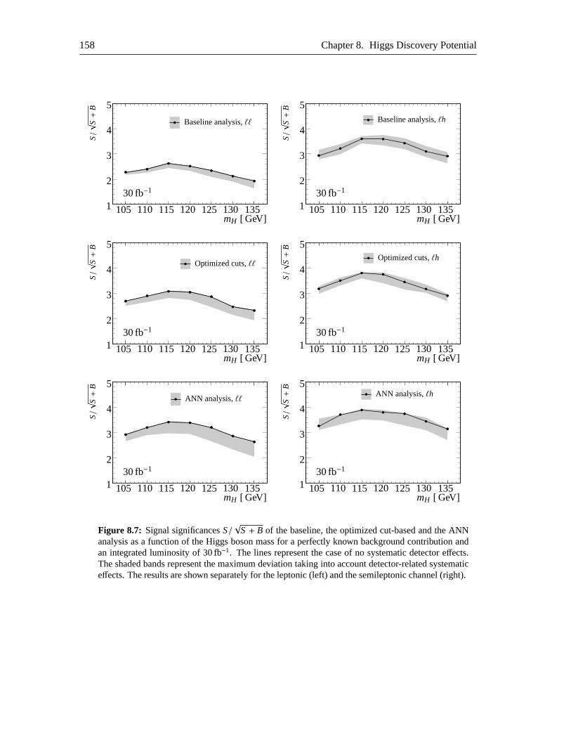
158 Chapter 8. Higgs Discovery Potential
1
2
3
4
5
105 110 115 120 125 130 135
ττ
mH [ GeV]
S/√
S+
B
Baseline analysis,ℓℓ
30 fb−1
1
2
3
4
5
105 110 115 120 125 130 135mH [ GeV]
S/√
S+
B
Baseline analysis,ℓh
30 fb−1
1
2
3
4
5
105 110 115 120 125 130 135mH [ GeV]
S/√
S+
B
Optimized cuts,ℓℓ
30 fb−1
1
2
3
4
5
105 110 115 120 125 130 135mH [ GeV]
S/√
S+
B
Optimized cuts,ℓh
30 fb−1
1
2
3
4
5
105 110 115 120 125 130 135
0.30
mH [ GeV]
S/√
S+
B
ANN analysis,ℓℓ
30 fb−1
1
2
3
4
5
105 110 115 120 125 130 135mH [ GeV]
S/√
S+
B
ANN analysis,ℓh
30 fb−1
Figure 8.7: Signal significancesS/√
S + B of the baseline, the optimized cut-based and the ANNanalysis as a function of the Higgs boson mass for a perfectlyknown background contribution andan integrated luminosity of 30 fb−1. The lines represent the case of no systematic detector effects.The shaded bands represent the maximum deviation taking into account detector-related systematiceffects. The results are shown separately for the leptonic (left) and the semileptonic channel (right).
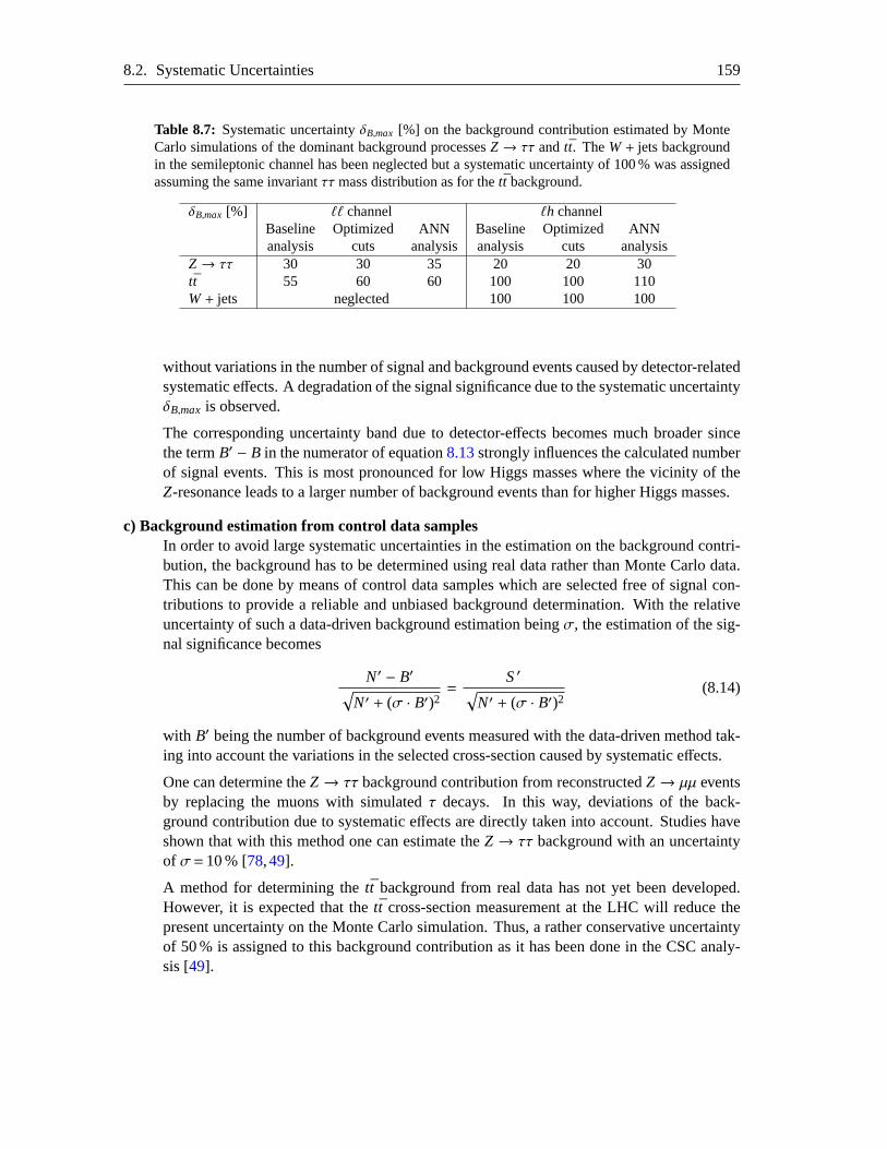
8.2. Systematic Uncertainties 159
Table 8.7: Systematic uncertaintyδB,max [%] on the background contribution estimated by MonteCarlo simulations of the dominant background processesZ→ ττ andtt. TheW+ jets backgroundin the semileptonic channel has been neglected but a systematic uncertainty of 100 % was assignedassuming the same invariantττmass distribution as for thett background.
δB,max [%] ℓℓ channel ℓh channelBaseline Optimized ANN Baseline Optimized ANNanalysis cuts analysis analysis cuts analysis
Z→ ττ 30 30 35 20 20 30tt 55 60 60 100 100 110W+ jets neglected 100 100 100
without variations in the number of signal and background events causedby detector-relatedsystematic effects. A degradation of the signal significance due to the systematic uncertaintyδB,max is observed.
The corresponding uncertainty band due to detector-effects becomes much broader sincethe termB′ − B in the numerator of equation8.13strongly influences the calculated numberof signal events. This is most pronounced for low Higgs masses where thevicinity of theZ-resonance leads to a larger number of background events than for higher Higgs masses.
c) Background estimation from control data samplesIn order to avoid large systematic uncertainties in the estimation on the background contri-bution, the background has to be determined using real data rather than Monte Carlo data.This can be done by means of control data samples which are selected freeof signal con-tributions to provide a reliable and unbiased background determination. With the relativeuncertainty of such a data-driven background estimation beingσ, the estimation of the sig-nal significance becomes
N′ − B′√
N′ + (σ · B′)2=
S′√
N′ + (σ · B′)2(8.14)
with B′ being the number of background events measured with the data-driven method tak-ing into account the variations in the selected cross-section caused by systematic effects.
One can determine theZ→ ττ background contribution from reconstructedZ→ µµ eventsby replacing the muons with simulatedτ decays. In this way, deviations of the back-ground contribution due to systematic effects are directly taken into account. Studies haveshown that with this method one can estimate theZ→ ττ background with an uncertaintyof σ=10 % [78,49].
A method for determining thett background from real data has not yet been developed.However, it is expected that thett cross-section measurement at the LHC will reduce thepresent uncertainty on the Monte Carlo simulation. Thus, a rather conservative uncertaintyof 50 % is assigned to this background contribution as it has been done in theCSC analy-sis [49].
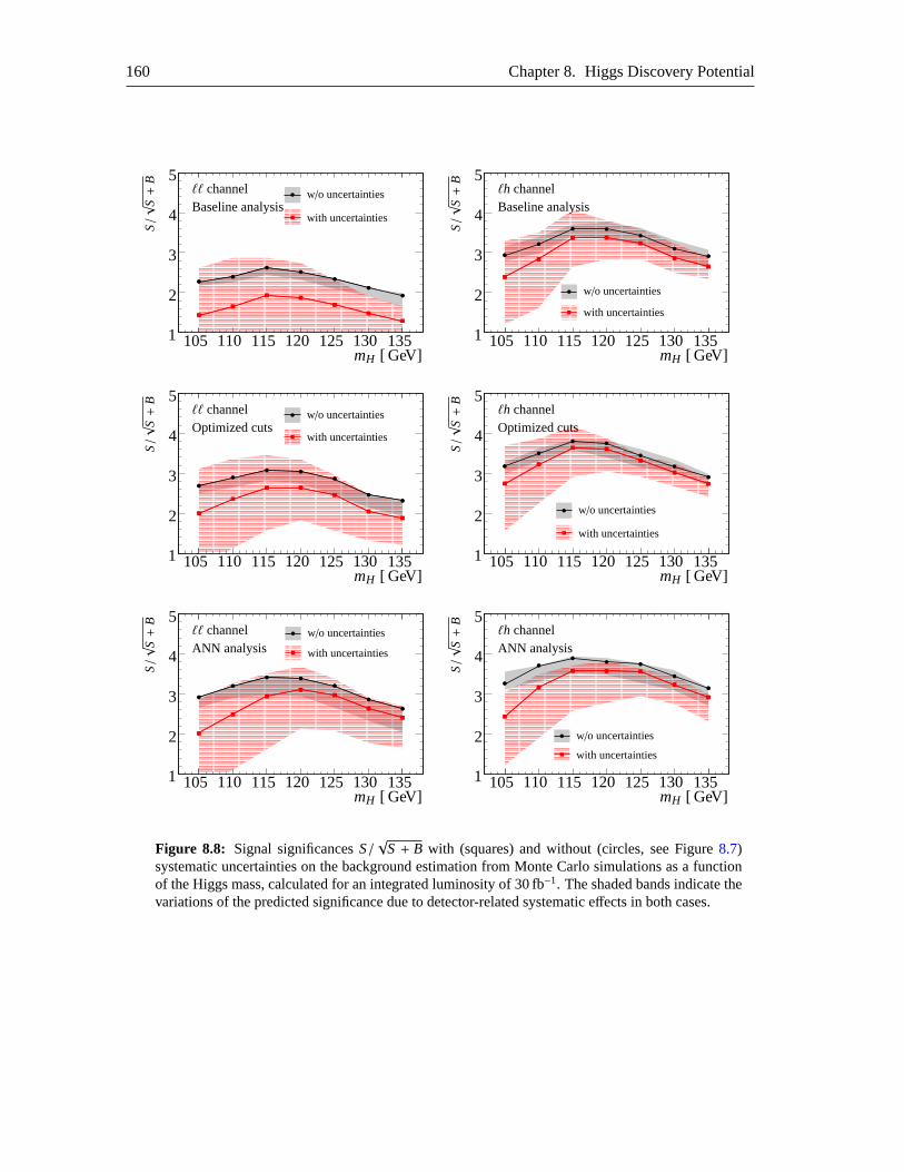
160 Chapter 8. Higgs Discovery Potential
1
2
3
4
5
105 110 115 120 125 130 135
+
mH [ GeV]
S/√
S+
B
w/o uncertainties
with uncertainties
ℓℓ channelBaseline analysis
1
2
3
4
5
105 110 115 120 125 130 135mH [ GeV]
S/√
S+
B
w/o uncertainties
with uncertainties
ℓh channelBaseline analysis
1
2
3
4
5
105 110 115 120 125 130 135
[ Ge
mH [ GeV]
S/√
S+
B
w/o uncertainties
with uncertainties
ℓℓ channelOptimized cuts
1
2
3
4
5
105 110 115 120 125 130 135mH [ GeV]
S/√
S+
B
w/o uncertainties
with uncertainties
ℓh channelOptimized cuts
1
2
3
4
5
105 110 115 120 125 130 135
ev
mH [ GeV]
S/√
S+
B
w/o uncertainties
with uncertainties
ℓℓ channelANN analysis
1
2
3
4
5
105 110 115 120 125 130 135mH [ GeV]
S/√
S+
B
w/o uncertainties
with uncertainties
ℓh channelANN analysis
Figure 8.8: Signal significancesS/√
S + B with (squares) and without (circles, see Figure8.7)systematic uncertainties on the background estimation from Monte Carlo simulations as a functionof the Higgs mass, calculated for an integrated luminosity of 30 fb−1. The shaded bands indicate thevariations of the predicted significance due to detector-related systematic effects in both cases.
8.2. Systematic Uncertainties 161
Figure8.9 shows the resulting predictions of the signal significance for the leptonic andsemileptonic channels and the analysis methods studied. The lines representthe signifi-cance predictions without systematic variations of signal and backgroundwhich are in turnindicated by the shaded bands.
Compared to the background estimation from Monte Carlo simulations (Figure8.8), theestimation of the background contribution by data-driven methods provideshigher signalsignificances and much narrower uncertainty bands. Thus, methods fora reliable estimationof the background from experimental data are crucial for a Higgs boson discovery in theH → ττ channel.
8.2.5 Profile Likelihood Calculation
For the case of data-driven background estimation, the signal significances have also been calcu-lated by means of the profile likelihood method (see Section8.1) in the same manner as it wasdone in the CSC analysis [49]. A simultaneous fit to themττ distributions of the signal candidatesas well as to theZ→ ττ and thett background estimations from data is performed with the sys-tematic uncertainties of 10 % and 50 % on theZ→ ττ andtt backgrounds being taken into accountin this calculation.The probability density functionsF(mττ; θ) for the signal and each background process havebeen determined from fits to the correspondingmττ distributions after all analysis cuts. BoththeZ→ ττ and the signal distribution are described by the sum of three Gaussians withidenticalmean and fixed ratios of the standard deviations (σ2 = 2.45 · σ1, σ3 = 5.02 · σ1) and normaliza-tions (N2 = 0.635· N1,N3 = 0.292· N1). In addition, an efficiency weighting function is used totake into account the asymmetry of theZ→ ττ andH → ττ resonances which is introduced bythe cuts on the visible momentum fractionsχ1,2 and on the missing transverse energyEmiss
T . It
is parameterized as 1/2+ 1/2 · erf{[mττ −mvis]/√
2σvis} where “erf” denotes the Gaussian errorfunction.mvis andσvis represent the mean and standard deviation of the distribution of the eventsrejected by theχ1,2 cuts, wheremvis is parameterized asmvis = 0.576mZ/H + 6.2 GeV andσvis isfixed to 10 GeV.Thus, the pdfs are:
FZ/H(mττ; mZ/H , σZ/H) = cn1
[
12+
12· erf
(
mττ −mvis√2σvis
)]
×3∑
i=1
Ni e(mττ−mZ/H)2/2σ2Z/H,i (8.15)
The shape of themττ distribution for thett background is parameterized by
Ftt(mττ; a1,a2,a3) = cn2
(
1mττ + a1
)a2
ma3ττ (8.16)
where the parameterscn1 andcn2 ensure the normalization of the pdfs.The pdf used for the fit to the signal candidates distribution is the sum of the pdfs of the threecontributions (signal,Z→ ττ andtt)
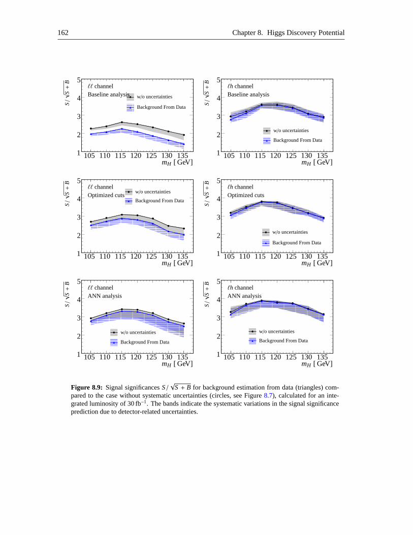
162 Chapter 8. Higgs Discovery Potential
1
2
3
4
5
105 110 115 120 125 130 135
+
mH [ GeV]
S/√
S+
B
w/o uncertainties
Background From Data
ℓℓ channelBaseline analysis
1
2
3
4
5
105 110 115 120 125 130 135mH [ GeV]
S/√
S+
B
w/o uncertainties
Background From Data
ℓh channelBaseline analysis
1
2
3
4
5
105 110 115 120 125 130 135
[ Ge
mH [ GeV]
S/√
S+
B
w/o uncertainties
Background From Data
ℓℓ channelOptimized cuts
1
2
3
4
5
105 110 115 120 125 130 135mH [ GeV]
S/√
S+
B
w/o uncertainties
Background From Data
ℓh channelOptimized cuts
1
2
3
4
5
105 110 115 120 125 130 135
ev
mH [ GeV]
S/√
S+
B
w/o uncertainties
Background From Data
ℓℓ channelANN analysis
1
2
3
4
5
105 110 115 120 125 130 135mH [ GeV]
S/√
S+
B
w/o uncertainties
Background From Data
ℓh channelANN analysis
Figure 8.9: Signal significancesS/√
S + B for background estimation from data (triangles) com-pared to the case without systematic uncertainties (circles, see Figure8.7), calculated for an inte-grated luminosity of 30 fb−1. The bands indicate the systematic variations in the signalsignificanceprediction due to detector-related uncertainties.
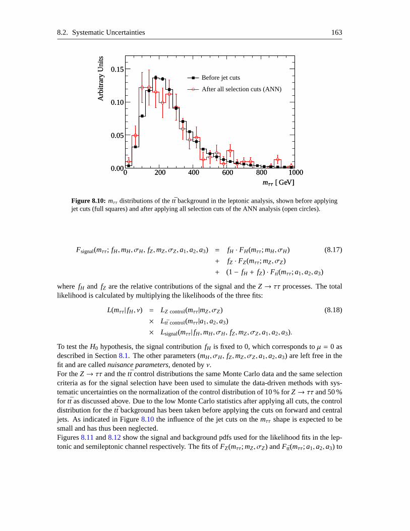
8.2. Systematic Uncertainties 163
00 200200 400400 600600 800800 100010000.000.00
0.050.05
0.100.10
0.150.15
Arb
itrar
yU
nits
Arb
itrar
yU
nits
mττ [ GeV]mττ [ GeV]
Before jet cuts
After all selection cuts (ANN)
Figure 8.10: mττ distributions of thett background in the leptonic analysis, shown before applyingjet cuts (full squares) and after applying all selection cuts of the ANN analysis (open circles).
Fsignal(mττ; fH ,mH , σH , fZ,mZ, σZ,a1,a2,a3) = fH · FH(mττ; mH , σH) (8.17)
+ fZ · FZ(mττ; mZ, σZ)
+ (1− fH + fZ) · Ftt(mττ; a1,a2,a3)
where fH and fZ are the relative contributions of the signal and theZ→ ττ processes. The totallikelihood is calculated by multiplying the likelihoods of the three fits:
L(mττ| fH , ν) = LZ control(mττ|mZ, σZ) (8.18)
× Ltt control(mττ|a1,a2,a3)
× Lsignal(mττ| fH ,mH , σH , fZ,mZ, σZ,a1,a2,a3).
To test theH0 hypothesis, the signal contributionfH is fixed to 0, which corresponds toµ = 0 asdescribed in Section8.1. The other parameters (mH , σH , fZ,mZ, σZ,a1,a2,a3) are left free in thefit and are callednuisance parameters, denoted byν.For theZ→ ττ and thett control distributions the same Monte Carlo data and the same selectioncriteria as for the signal selection have been used to simulate the data-driven methods with sys-tematic uncertainties on the normalization of the control distribution of 10 % forZ→ ττ and 50 %for tt as discussed above. Due to the low Monte Carlo statistics after applying all cuts, the controldistribution for thett background has been taken before applying the cuts on forward and centraljets. As indicated in Figure8.10the influence of the jet cuts on themττ shape is expected to besmall and has thus been neglected.Figures8.11and8.12show the signal and background pdfs used for the likelihood fits in the lep-tonic and semileptonic channel respectively. The fits ofFZ(mττ; mZ, σZ) andFtt(mττ; a1,a2,a3) to
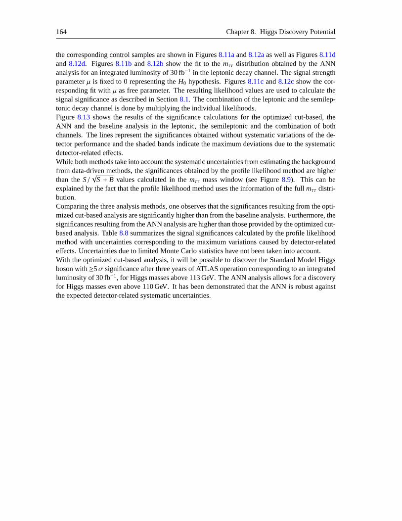
164 Chapter 8. Higgs Discovery Potential
the corresponding control samples are shown in Figures8.11aand8.12aas well as Figures8.11dand8.12d. Figures8.11band8.12bshow the fit to themττ distribution obtained by the ANNanalysis for an integrated luminosity of 30 fb−1 in the leptonic decay channel. The signal strengthparameterµ is fixed to 0 representing theH0 hypothesis. Figures8.11cand8.12cshow the cor-responding fit withµ as free parameter. The resulting likelihood values are used to calculate thesignal significance as described in Section8.1. The combination of the leptonic and the semilep-tonic decay channel is done by multiplying the individual likelihoods.Figure 8.13 shows the results of the significance calculations for the optimized cut-based, theANN and the baseline analysis in the leptonic, the semileptonic and the combination of bothchannels. The lines represent the significances obtained without systematic variations of the de-tector performance and the shaded bands indicate the maximum deviations dueto the systematicdetector-related effects.While both methods take into account the systematic uncertainties from estimating thebackgroundfrom data-driven methods, the significances obtained by the profile likelihood method are higherthan theS/
√S + B values calculated in themττ mass window (see Figure8.9). This can be
explained by the fact that the profile likelihood method uses the information of the full mττ distri-bution.Comparing the three analysis methods, one observes that the significancesresulting from the opti-mized cut-based analysis are significantly higher than from the baseline analysis. Furthermore, thesignificances resulting from the ANN analysis are higher than those provided by the optimized cut-based analysis. Table8.8summarizes the signal significances calculated by the profile likelihoodmethod with uncertainties corresponding to the maximum variations caused by detector-relatedeffects. Uncertainties due to limited Monte Carlo statistics have not been taken into account.With the optimized cut-based analysis, it will be possible to discover the Standard Model Higgsboson with≥5σ significance after three years of ATLAS operation corresponding to anintegratedluminosity of 30 fb−1, for Higgs masses above 113 GeV. The ANN analysis allows for a discoveryfor Higgs masses even above 110 GeV. It has been demonstrated that theANN is robust againstthe expected detector-related systematic uncertainties.
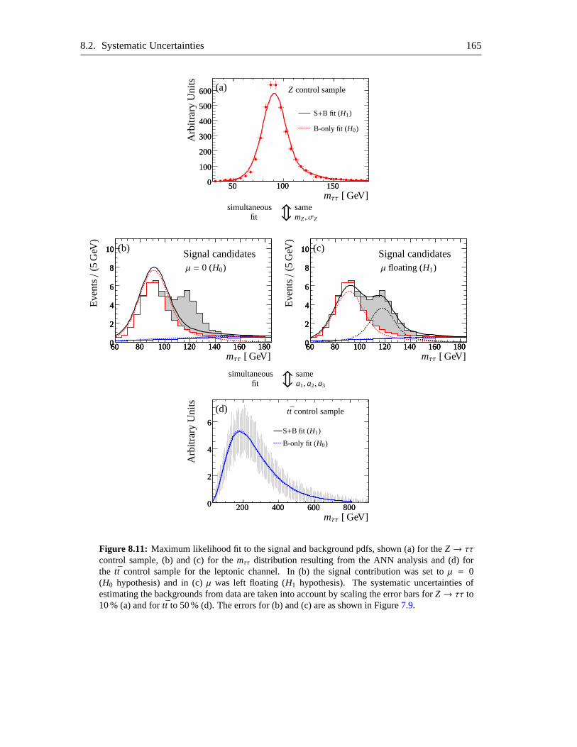
8.2. Systematic Uncertainties 165
00 5050
100
100
100
100 150150
200200
300300
400400
500500
600600
Arb
itrar
yU
nits
mττ [ GeV]
(a) Z control sample
S+B fit (H1)
B-only fit (H0)
simultaneousfit m same
mZ, σZ
000
222
444
666
888
101010
606060 808080 100100100 120120120 140140140 160160160 180180180
∆
mττ [ GeV]
Eve
nts/
(5G
eV)
(b)Signal candidatesµ = 0 (H0)
000
222
444
666
888
101010
606060 808080 100100100 120120120 140140140 160160160 180180180mττ [ GeV]
Eve
nts/
(5G
eV)
(c)Signal candidatesµ floating (H1)
simultaneousfit m same
a1,a2,a3
00
22
44
66
200200 400400 600600 800800mττ [ GeV]
Arb
itrar
yU
nits
tt control sample
S+B fit (H1)
B-only fit (H0)
(d)
Figure 8.11: Maximum likelihood fit to the signal and background pdfs, shown (a) for theZ→ ττcontrol sample, (b) and (c) for themττ distribution resulting from the ANN analysis and (d) forthe tt control sample for the leptonic channel. In (b) the signal contribution was set toµ = 0(H0 hypothesis) and in (c)µ was left floating (H1 hypothesis). The systematic uncertainties ofestimating the backgrounds from data are taken into accountby scaling the error bars forZ→ ττ to10 % (a) and fortt to 50 % (d). The errors for (b) and (c) are as shown in Figure7.9.
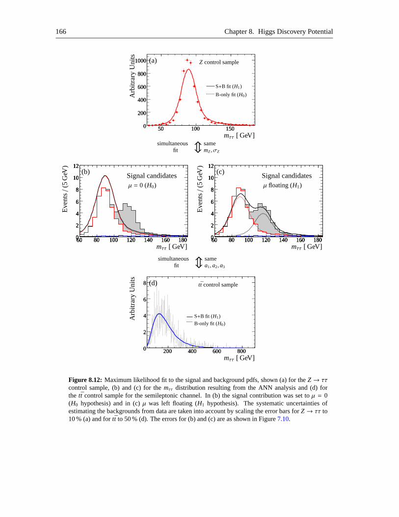
166 Chapter 8. Higgs Discovery Potential
00 5050 100100 150150
200200
400400
600600
800800
10001000
Arb
itrar
yU
nits
mττ [ GeV]
(a) Z control sample
S+B fit (H1)
B-only fit (H0)
simultaneousfit m same
mZ, σZ
000
222
444
666
888
101010
121212
606060 808080 100100100 120120120 140140140 160160160 180180180
∆
mττ [ GeV]
Eve
nts/
(5G
eV)
(b)Signal candidatesµ = 0 (H0)
000
222
444
666
888
101010
121212
606060 808080 100100100 120120120 140140140 160160160 180180180mττ [ GeV]
Eve
nts/
(5G
eV)
(c)Signal candidatesµ floating (H1)
simultaneousfit m same
a1,a2,a3
00
22
44
66
88
200200 400400 600600 800800mττ [ GeV]
Arb
itrar
yU
nits
tt control sample
S+B fit (H1)
B-only fit (H0)
(d)
Figure 8.12: Maximum likelihood fit to the signal and background pdfs, shown (a) for theZ→ ττcontrol sample, (b) and (c) for themττ distribution resulting from the ANN analysis and (d) forthe tt control sample for the semileptonic channel. In (b) the signal contribution was set toµ = 0(H0 hypothesis) and in (c)µ was left floating (H1 hypothesis). The systematic uncertainties ofestimating the backgrounds from data are taken into accountby scaling the error bars forZ→ ττ to10 % (a) and fortt to 50 % (d). The errors for (b) and (c) are as shown in Figure7.10.
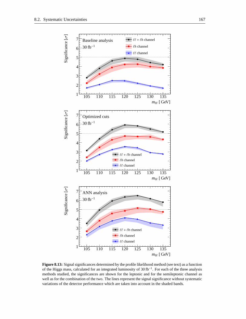
8.2. Systematic Uncertainties 167
1
2
3
4
5
6
7
105 110 115 120 125 130 135mH [ GeV]
Sig
nific
ance
[σ]
ℓℓ + ℓh channel
ℓℓ channel
ℓh channel30 fb−1
Baseline analysis
1
2
3
4
5
6
7
105 110 115 120 125 130 135mH [ GeV]
Sig
nific
ance
[σ]
ℓℓ + ℓh channel
ℓℓ channel
ℓh channel
30 fb−1
Optimized cuts
1
2
3
4
5
6
7
105 110 115 120 125 130 135mH [ GeV]
Sig
nific
ance
[σ]
ℓℓ + ℓh channel
ℓℓ channel
ℓh channel
30 fb−1
ANN analysis
Figure 8.13: Signal significances determined by the profile likelihood method (see text) as a functionof the Higgs mass, calculated for an integrated luminosity of 30 fb−1. For each of the three analysismethods studied, the significances are shown for the leptonic and for the semileptonic channel aswell as for the combination of the two. The lines represent the signal significance without systematicvariations of the detector performance which are taken intoaccount in the shaded bands.
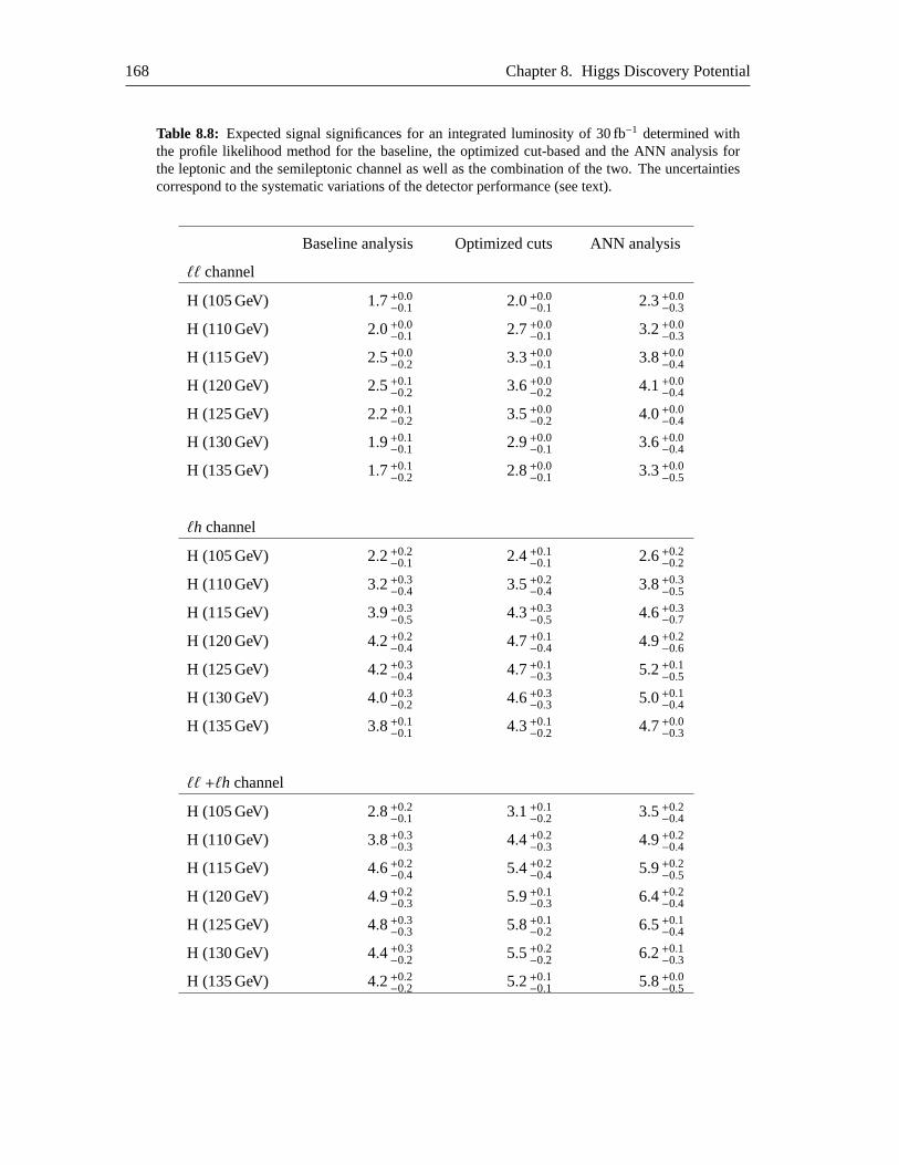
168 Chapter 8. Higgs Discovery Potential
Table 8.8: Expected signal significances for an integrated luminosityof 30 fb−1 determined withthe profile likelihood method for the baseline, the optimized cut-based and the ANN analysis forthe leptonic and the semileptonic channel as well as the combination of the two. The uncertaintiescorrespond to the systematic variations of the detector performance (see text).
Baseline analysis Optimized cuts ANN analysis
ℓℓ channel
H (105 GeV) 1.7+0.0−0.1 2.0+0.0
−0.1 2.3+0.0−0.3
H (110 GeV) 2.0+0.0−0.1 2.7+0.0
−0.1 3.2+0.0−0.3
H (115 GeV) 2.5+0.0−0.2 3.3+0.0
−0.1 3.8+0.0−0.4
H (120 GeV) 2.5+0.1−0.2 3.6+0.0
−0.2 4.1+0.0−0.4
H (125 GeV) 2.2+0.1−0.2 3.5+0.0
−0.2 4.0+0.0−0.4
H (130 GeV) 1.9+0.1−0.1 2.9+0.0
−0.1 3.6+0.0−0.4
H (135 GeV) 1.7+0.1−0.2 2.8+0.0
−0.1 3.3+0.0−0.5
ℓh channel
H (105 GeV) 2.2+0.2−0.1 2.4+0.1
−0.1 2.6+0.2−0.2
H (110 GeV) 3.2+0.3−0.4 3.5+0.2
−0.4 3.8+0.3−0.5
H (115 GeV) 3.9+0.3−0.5 4.3+0.3
−0.5 4.6+0.3−0.7
H (120 GeV) 4.2+0.2−0.4 4.7+0.1
−0.4 4.9+0.2−0.6
H (125 GeV) 4.2+0.3−0.4 4.7+0.1
−0.3 5.2+0.1−0.5
H (130 GeV) 4.0+0.3−0.2 4.6+0.3
−0.3 5.0+0.1−0.4
H (135 GeV) 3.8+0.1−0.1 4.3+0.1
−0.2 4.7+0.0−0.3
ℓℓ +ℓh channel
H (105 GeV) 2.8+0.2−0.1 3.1+0.1
−0.2 3.5+0.2−0.4
H (110 GeV) 3.8+0.3−0.3 4.4+0.2
−0.3 4.9+0.2−0.4
H (115 GeV) 4.6+0.2−0.4 5.4+0.2
−0.4 5.9+0.2−0.5
H (120 GeV) 4.9+0.2−0.3 5.9+0.1
−0.3 6.4+0.2−0.4
H (125 GeV) 4.8+0.3−0.3 5.8+0.1
−0.2 6.5+0.1−0.4
H (130 GeV) 4.4+0.3−0.2 5.5+0.2
−0.2 6.2+0.1−0.3
H (135 GeV) 4.2+0.2−0.2 5.2+0.1
−0.1 5.8+0.0−0.5
Chapter 9
Summary
The ATLAS experiment at the Large Hadron Collider is designed to explore awide range of newphenomena in particle physics with proton-proton collisions at energies up to14 TeV. An integralpart of the ATLAS detector is the muon spectrometer for which the Max-Planck-Institut fur Physikin Munich in collaboration with the Ludwig-Maximilians University has built 88 precision driftchambers. The installation of the muon chambers in the ATLAS cavern took place in the years2005 – 2007. Almost 1 200 chambers had to be positioned with an accuracy of 1 mm with respectto the interaction point.
Gas leak and high voltage tests have been carried out before and after installation in order to detectpossible damages during installation. Afterwards, the performance of the muon spectrometer hasbeen tested with cosmic ray muons. An average muon detection efficiency of the drift tubes of97 % has been measured in agreement with the expectation. A part of the barrel muon chambershas been aligned with muon tracks with the desired accuracy in the regions where a sufficientnumber of cosmic muons could be detected.
The muon spectrometer performance has an important impact on searches for Higgs decays withmuons in the final state. The discovery of the Higgs boson is the main objectiveof the ATLASexperiment. Experimental and theoretical bounds constrain the Standard Model Higgs boson massto the range 114.4 GeV≤mH ≤185 GeV. One of the most promising discovery channel in this massrange is the vector-boson fusion production of the Higgs boson with the subsequent decay into aτ-lepton pair. The decay modes where bothτ leptons decay leptonically or where oneτ leptondecays leptonically and the other one hadronically have been studied. TheHiggs boson mass canbe reconstructed with a resolution of about 10 GeV in this channel.
Various discriminating variables can be used to suppress the dominant backgrounds from top quarkpair tt andZ boson production and decay toτ leptons. The vector-boson fusion process is charac-terized by two highly energetic jets in the forward regions of the detector providing a particularlyimportant signature for Higgs detection in this production process.
Two signal selection methods have been studied in this work, a cut-based analysis and a mul-tivariate analysis method. In the case of the cut-based analysis, the discovery potential of thesearch channel is significantly increased compared to previously published results by using addi-tional discriminating variables and optimizing the selection cuts by an iterative procedure. Whilethe signal efficiency remained unchanged the background suppression improved significantly, in
169

170 Chapter 9. Summary
particular for thett background contribution to the leptonic channel which could be reduced byapproximately 70 %.In order to fully take into account correlations between the discriminating variables, the multivari-ate analysis methods Projective Likelihood, Fisher Linear Discriminant, Boosted Decision Treesand Artificial Neural Networks have been studied. The input variables have been carefully selectedin order to obtain best discrimination while avoiding any bias of the reconstructed Higgs bosonmass distribution.The Artificial Neural Network algorithm showed the best performance in terms of achievable sig-nal significance including systematic uncertainties and stability of the results withrespect to thechoice of discriminating variables. The background suppression of the Artificial Neural Networkanalysis is similar to the optimized cut-based analysis while the signal efficiency is further in-creased by approximately 10 % for all tested Higgs boson masses in the studied range from 105 to135 GeV, although the network has only been trained for a Higgs mass of 120 GeV.The impact of systematic uncertainties, in particular the simulated detector performance has beendiscussed. The largest systematic effect on the selection efficiencies for signal and background isthe uncertainty in the jet energy calibration. Both the cut-based and the Artificial Neural Networkanalysis show a similar sensitivity to the systematic uncertainties. Their impact on the expectedHiggs discovery potential shows the need for a reliable determination of the background contribu-tions from the data rather than from Monte Carlo simulations.The final results for the signal significance for the leptonic and semileptonicchannel as well asfor the combination of the two are derived from a maximum likelihood fit to theτ-pair invariantmass spectra for signal and background using a profile likelihood ratio method and assumingbackground estimation from data with uncertainties of 10 % for theZ→ ττ and 50 % for thettbackground.Combining both channels one can expect to discover the Higgs boson with≥5σ significance inthe mass range 115 GeV≤mH ≤135 GeV and a maximum signal significance of 5.9σ for a Higgsmass of 120 GeV with an integrated luminosity of 30 fb−1 corresponding to the first three years ofATLAS operation. With the Artificial Neural Network method, the mass range for ≥5σ Higgsdiscovery with 30 fb−1 is extended down to 110 GeV with a maximum signal significance of 6.5σ
for mH =125 GeV. For both analyses, the systematic uncertainty in the prediction of thesignalsignificance is approximately 10 %.

Appendix A
Details for all Higgs Masses
On the following pages, the evolution of the cross-sections with the applied analysis cuts are shownfor all studied Higgs mass datasets for the cut-based and the multivariate analysis and for both theleptonic and the semileptonic decay channel.
171
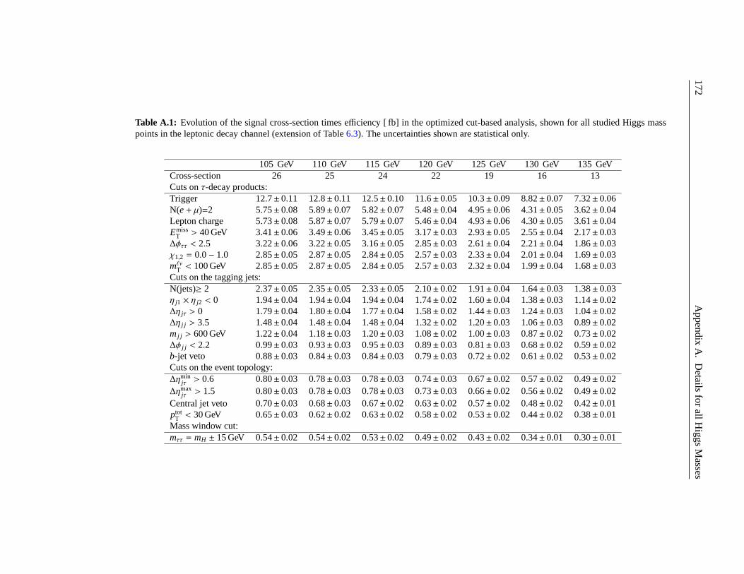
172A
ppendixA
.D
etailsfor
allHiggs
Masses
Table A.1: Evolution of the signal cross-section times efficiency [ fb] in the optimized cut-based analysis, shown for all studied Higgs masspoints in the leptonic decay channel (extension of Table6.3). The uncertainties shown are statistical only.
105 GeV 110 GeV 115 GeV 120 GeV 125 GeV 130 GeV 135 GeVCross-section 26 25 24 22 19 16 13Cuts onτ-decay products:Trigger 12.7± 0.11 12.8± 0.11 12.5±0.10 11.6±0.05 10.3± 0.09 8.82± 0.07 7.32± 0.06N(e+ µ)=2 5.75± 0.08 5.89± 0.07 5.82±0.07 5.48±0.04 4.95± 0.06 4.31± 0.05 3.62± 0.04Lepton charge 5.73± 0.08 5.87± 0.07 5.79±0.07 5.46±0.04 4.93± 0.06 4.30± 0.05 3.61± 0.04Emiss
T > 40 GeV 3.41± 0.06 3.49± 0.06 3.45±0.05 3.17±0.03 2.93± 0.05 2.55± 0.04 2.17± 0.03∆φττ < 2.5 3.22± 0.06 3.22± 0.05 3.16±0.05 2.85±0.03 2.61± 0.04 2.21± 0.04 1.86± 0.03χ1,2 = 0.0− 1.0 2.85± 0.05 2.87± 0.05 2.84±0.05 2.57±0.03 2.33± 0.04 2.01± 0.04 1.69± 0.03mℓνT < 100 GeV 2.85± 0.05 2.87± 0.05 2.84±0.05 2.57±0.03 2.32± 0.04 1.99± 0.04 1.68± 0.03Cuts on the tagging jets:N(jets)≥ 2 2.37± 0.05 2.35± 0.05 2.33±0.05 2.10±0.02 1.91± 0.04 1.64± 0.03 1.38± 0.03η j1 × η j2 < 0 1.94± 0.04 1.94± 0.04 1.94±0.04 1.74±0.02 1.60± 0.04 1.38± 0.03 1.14± 0.02∆η jτ > 0 1.79± 0.04 1.80± 0.04 1.77±0.04 1.58±0.02 1.44± 0.03 1.24± 0.03 1.04± 0.02∆η j j > 3.5 1.48± 0.04 1.48± 0.04 1.48±0.04 1.32±0.02 1.20± 0.03 1.06± 0.03 0.89± 0.02mj j > 600 GeV 1.22± 0.04 1.18± 0.03 1.20±0.03 1.08±0.02 1.00± 0.03 0.87± 0.02 0.73± 0.02∆φ j j < 2.2 0.99± 0.03 0.93± 0.03 0.95±0.03 0.89±0.03 0.81± 0.03 0.68± 0.02 0.59± 0.02b-jet veto 0.88± 0.03 0.84± 0.03 0.84±0.03 0.79±0.03 0.72± 0.02 0.61± 0.02 0.53± 0.02Cuts on the event topology:∆ηmin
jτ > 0.6 0.80± 0.03 0.78± 0.03 0.78±0.03 0.74±0.03 0.67± 0.02 0.57± 0.02 0.49± 0.02∆ηmax
jτ > 1.5 0.80± 0.03 0.78± 0.03 0.78±0.03 0.73±0.03 0.66± 0.02 0.56± 0.02 0.49± 0.02Central jet veto 0.70± 0.03 0.68± 0.03 0.67±0.02 0.63±0.02 0.57± 0.02 0.48± 0.02 0.42± 0.01ptot
T < 30 GeV 0.65± 0.03 0.62± 0.02 0.63±0.02 0.58±0.02 0.53± 0.02 0.44± 0.02 0.38± 0.01Mass window cut:mττ = mH ± 15 GeV 0.54± 0.02 0.54± 0.02 0.53±0.02 0.49±0.02 0.43± 0.02 0.34± 0.01 0.30± 0.01
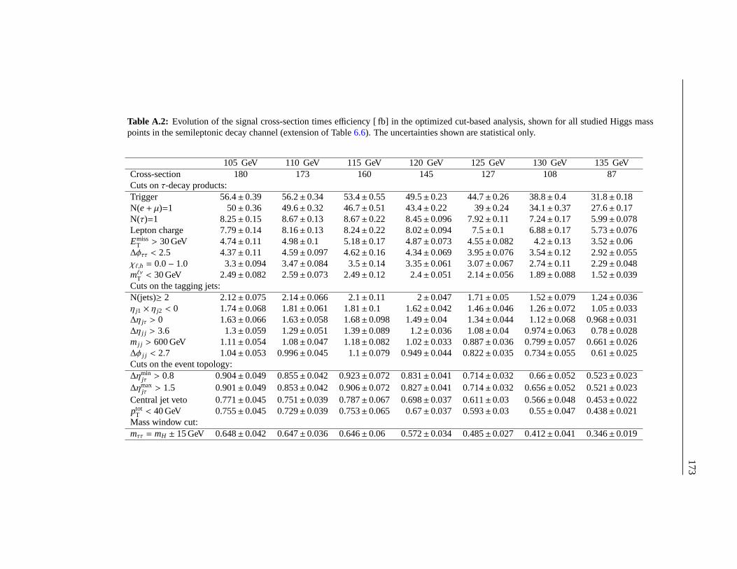
173
Table A.2: Evolution of the signal cross-section times efficiency [ fb] in the optimized cut-based analysis, shown for all studied Higgs masspoints in the semileptonic decay channel (extension of Table 6.6). The uncertainties shown are statistical only.
105 GeV 110 GeV 115 GeV 120 GeV 125 GeV 130 GeV 135 GeVCross-section 180 173 160 145 127 108 87Cuts onτ-decay products:Trigger 56.4±0.39 56.2± 0.34 53.4± 0.55 49.5±0.23 44.7±0.26 38.8± 0.4 31.8± 0.18N(e+ µ)=1 50±0.36 49.6± 0.32 46.7± 0.51 43.4±0.22 39±0.24 34.1± 0.37 27.6± 0.17N(τ)=1 8.25±0.15 8.67± 0.13 8.67± 0.22 8.45±0.096 7.92±0.11 7.24± 0.17 5.99± 0.078Lepton charge 7.79±0.14 8.16± 0.13 8.24± 0.22 8.02±0.094 7.5±0.1 6.88± 0.17 5.73± 0.076Emiss
T > 30 GeV 4.74±0.11 4.98± 0.1 5.18± 0.17 4.87±0.073 4.55±0.082 4.2± 0.13 3.52± 0.06∆φττ < 2.5 4.37±0.11 4.59± 0.097 4.62± 0.16 4.34±0.069 3.95±0.076 3.54± 0.12 2.92± 0.055χℓ,h = 0.0− 1.0 3.3±0.094 3.47± 0.084 3.5± 0.14 3.35±0.061 3.07±0.067 2.74± 0.11 2.29± 0.048mℓνT < 30 GeV 2.49±0.082 2.59± 0.073 2.49± 0.12 2.4±0.051 2.14±0.056 1.89± 0.088 1.52± 0.039Cuts on the tagging jets:N(jets)≥ 2 2.12±0.075 2.14± 0.066 2.1± 0.11 2±0.047 1.71±0.05 1.52± 0.079 1.24± 0.036η j1 × η j2 < 0 1.74±0.068 1.81± 0.061 1.81± 0.1 1.62±0.042 1.46±0.046 1.26± 0.072 1.05± 0.033∆η jτ > 0 1.63±0.066 1.63± 0.058 1.68± 0.098 1.49±0.04 1.34±0.044 1.12± 0.068 0.968± 0.031∆η j j > 3.6 1.3±0.059 1.29± 0.051 1.39± 0.089 1.2±0.036 1.08±0.04 0.974± 0.063 0.78± 0.028mj j > 600 GeV 1.11±0.054 1.08± 0.047 1.18± 0.082 1.02±0.033 0.887±0.036 0.799± 0.057 0.661± 0.026∆φ j j < 2.7 1.04±0.053 0.996± 0.045 1.1± 0.079 0.949±0.044 0.822±0.035 0.734± 0.055 0.61± 0.025Cuts on the event topology:∆ηmin
jτ > 0.8 0.904±0.049 0.855± 0.042 0.923± 0.072 0.831±0.041 0.714±0.032 0.66± 0.052 0.523± 0.023∆ηmax
jτ > 1.5 0.901±0.049 0.853± 0.042 0.906± 0.072 0.827±0.041 0.714±0.032 0.656± 0.052 0.521± 0.023Central jet veto 0.771±0.045 0.751± 0.039 0.787± 0.067 0.698±0.037 0.611±0.03 0.566± 0.048 0.453± 0.022ptot
T < 40 GeV 0.755±0.045 0.729± 0.039 0.753± 0.065 0.67±0.037 0.593±0.03 0.55± 0.047 0.438± 0.021Mass window cut:mττ = mH ± 15 GeV 0.648±0.042 0.647± 0.036 0.646± 0.06 0.572±0.034 0.485±0.027 0.412± 0.041 0.346± 0.019
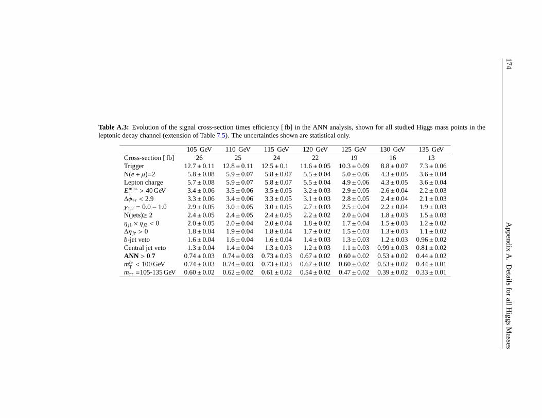
174A
ppendixA
.D
etailsfor
allHiggs
Masses
Table A.3: Evolution of the signal cross-section times efficiency [ fb] in the ANN analysis, shown for all studied Higgs mass points in theleptonic decay channel (extension of Table7.5). The uncertainties shown are statistical only.
105 GeV 110 GeV 115 GeV 120 GeV 125 GeV 130 GeV 135 GeVCross-section [ fb] 26 25 24 22 19 16 13Trigger 12.7±0.11 12.8± 0.11 12.5± 0.1 11.6± 0.05 10.3±0.09 8.8±0.07 7.3± 0.06N(e+ µ)=2 5.8±0.08 5.9± 0.07 5.8± 0.07 5.5± 0.04 5.0±0.06 4.3±0.05 3.6± 0.04Lepton charge 5.7±0.08 5.9± 0.07 5.8± 0.07 5.5± 0.04 4.9±0.06 4.3±0.05 3.6± 0.04Emiss
T > 40 GeV 3.4±0.06 3.5± 0.06 3.5± 0.05 3.2± 0.03 2.9±0.05 2.6±0.04 2.2± 0.03∆φττ < 2.9 3.3±0.06 3.4± 0.06 3.3± 0.05 3.1± 0.03 2.8±0.05 2.4±0.04 2.1± 0.03χ1,2 = 0.0− 1.0 2.9±0.05 3.0± 0.05 3.0± 0.05 2.7± 0.03 2.5±0.04 2.2±0.04 1.9± 0.03N(jets)≥ 2 2.4±0.05 2.4± 0.05 2.4± 0.05 2.2± 0.02 2.0±0.04 1.8±0.03 1.5± 0.03η j1 × η j2 < 0 2.0±0.05 2.0± 0.04 2.0± 0.04 1.8± 0.02 1.7±0.04 1.5±0.03 1.2± 0.02∆η jτ > 0 1.8±0.04 1.9± 0.04 1.8± 0.04 1.7± 0.02 1.5±0.03 1.3±0.03 1.1± 0.02b-jet veto 1.6±0.04 1.6± 0.04 1.6± 0.04 1.4± 0.03 1.3±0.03 1.2±0.03 0.96± 0.02Central jet veto 1.3±0.04 1.4± 0.04 1.3± 0.03 1.2± 0.03 1.1±0.03 0.99±0.03 0.81± 0.02ANN > 0.7 0.74±0.03 0.74± 0.03 0.73± 0.03 0.67± 0.02 0.60±0.02 0.53±0.02 0.44± 0.02mℓνT < 100 GeV 0.74±0.03 0.74± 0.03 0.73± 0.03 0.67± 0.02 0.60±0.02 0.53±0.02 0.44± 0.01mττ =105-135 GeV 0.60±0.02 0.62± 0.02 0.61± 0.02 0.54± 0.02 0.47±0.02 0.39±0.02 0.33± 0.01
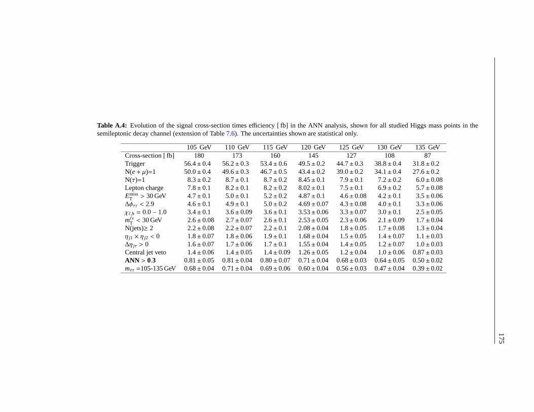
175
Table A.4: Evolution of the signal cross-section times efficiency [ fb] in the ANN analysis, shown for all studied Higgs mass points in thesemileptonic decay channel (extension of Table7.6). The uncertainties shown are statistical only.
105 GeV 110 GeV 115 GeV 120 GeV 125 GeV 130 GeV 135 GeVCross-section [ fb] 180 173 160 145 127 108 87Trigger 56.4± 0.4 56.2± 0.3 53.4± 0.6 49.5±0.2 44.7±0.3 38.8± 0.4 31.8± 0.2N(e+ µ)=1 50.0± 0.4 49.6± 0.3 46.7± 0.5 43.4±0.2 39.0±0.2 34.1± 0.4 27.6± 0.2N(τ)=1 8.3± 0.2 8.7± 0.1 8.7± 0.2 8.45±0.1 7.9±0.1 7.2± 0.2 6.0± 0.08Lepton charge 7.8± 0.1 8.2± 0.1 8.2± 0.2 8.02±0.1 7.5±0.1 6.9± 0.2 5.7± 0.08Emiss
T > 30 GeV 4.7± 0.1 5.0± 0.1 5.2± 0.2 4.87±0.1 4.6±0.08 4.2± 0.1 3.5± 0.06∆φττ < 2.9 4.6± 0.1 4.9± 0.1 5.0± 0.2 4.69±0.07 4.3±0.08 4.0± 0.1 3.3± 0.06χℓ,h = 0.0− 1.0 3.4± 0.1 3.6± 0.09 3.6± 0.1 3.53±0.06 3.3±0.07 3.0± 0.1 2.5± 0.05mℓνT < 30 GeV 2.6± 0.08 2.7± 0.07 2.6± 0.1 2.53±0.05 2.3±0.06 2.1± 0.09 1.7± 0.04N(jets)≥ 2 2.2± 0.08 2.2± 0.07 2.2± 0.1 2.08±0.04 1.8±0.05 1.7± 0.08 1.3± 0.04η j1 × η j2 < 0 1.8± 0.07 1.8± 0.06 1.9± 0.1 1.68±0.04 1.5±0.05 1.4± 0.07 1.1± 0.03∆η jτ > 0 1.6± 0.07 1.7± 0.06 1.7± 0.1 1.55±0.04 1.4±0.05 1.2± 0.07 1.0± 0.03Central jet veto 1.4± 0.06 1.4± 0.05 1.4± 0.09 1.26±0.05 1.2±0.04 1.0± 0.06 0.87± 0.03ANN > 0.3 0.81± 0.05 0.81± 0.04 0.80± 0.07 0.71±0.04 0.68±0.03 0.64± 0.05 0.50± 0.02mττ =105-135 GeV 0.68± 0.04 0.71± 0.04 0.69± 0.06 0.60±0.04 0.56±0.03 0.47± 0.04 0.39± 0.02

List of Figures
2.1 The Higgs potential.. . . . . . . . . . . . . . . . . . . . . . . . . . . . . . . . . 52.2 Upper and lower theoretical bounds on the Higgs boson mass.. . . . . . . . . . 72.3 ∆χ2 from the fit to electroweak data.. . . . . . . . . . . . . . . . . . . . . . . . 92.4 Tree-level Feynman diagrams of the Higgs boson production processes in proton-
proton collisions at the LHC.. . . . . . . . . . . . . . . . . . . . . . . . . . . . 102.5 Standard Model Higgs boson production cross-sections.. . . . . . . . . . . . . . 112.6 Feynman diagrams of the Higgs boson decay channels.. . . . . . . . . . . . . . 112.7 Branching ratios of the Higgs boson.. . . . . . . . . . . . . . . . . . . . . . . . 12
3.1 Schematic picture of the LHC at CERN with the experiments at the four interactionpoints. . . . . . . . . . . . . . . . . . . . . . . . . . . . . . . . . . . . . . . . . 16
3.2 Cut-away view of the ATLAS detector.. . . . . . . . . . . . . . . . . . . . . . . 193.3 Sketch of the ATLAS magnet system.. . . . . . . . . . . . . . . . . . . . . . . 203.4 Cut-away view of the ATLAS inner detector.. . . . . . . . . . . . . . . . . . . . 213.5 Cut-away view of the ATLAS calorimeter system.. . . . . . . . . . . . . . . . . 223.6 Cut-away view of the ATLAS Muon Spectrometer.. . . . . . . . . . . . . . . . 243.7 Cross-sections of the barrel muon system.. . . . . . . . . . . . . . . . . . . . . 243.8 Layout of a MDT chamber. Three cross-plates connected by longitudinal beams
form an aluminum support structure, carrying two multilayers of three or four drifttube layers. Four optical alignment rays monitor deformations of the chamber. . 25
4.1 Pictures of the muon chamber installation.. . . . . . . . . . . . . . . . . . . . . 284.2 Front view of the barrel part of the ATLAS muon spectrometer after theinstallation
of the muon chambers on the eight toroid coils. The BOS MDT chambers built inMunich are mounted in the outer layer of the muon spectrometer, directly on thetoroid coils. . . . . . . . . . . . . . . . . . . . . . . . . . . . . . . . . . . . . . 29
4.3 Deviation of the chamber positions from the nominal positions, shown for onesector of the BOS chambers.. . . . . . . . . . . . . . . . . . . . . . . . . . . . 30
4.4 Principle and accuracy of the adjustment of the gravitational sag of the drift tubesand the anode wires.. . . . . . . . . . . . . . . . . . . . . . . . . . . . . . . . 31
4.5 Single-tube efficiencies in one tube layer of a MDT chamber installed in theATLAS detector determined with cosmic muons.. . . . . . . . . . . . . . . . . 34
177
178 LIST OF FIGURES
4.7 Illustration of the track sagitta measurement performed in the ATLAS barrel muonspectrometer. . . . . . . . . . . . . . . . . . . . . . . . . . . . . . . . . . . . . 35
4.8 Comparison of the distances between adjacent chambers in the inner andouterlayer of the top sector of the muon spectrometer as determined by mechanicalmeasurements with a feeler gauge and by the straight track alignment algorithm.. 37
4.9 Distributions of the measured sagitta of straight cosmic muon tracks in the ATLASmuon spectrometer without magnetic field.. . . . . . . . . . . . . . . . . . . . . 37
4.10 Display of events with reconstructed low momentum and high momentum cosmicmuons.. . . . . . . . . . . . . . . . . . . . . . . . . . . . . . . . . . . . . . . . 38
4.11 Cosmic muon momentum spectrum.. . . . . . . . . . . . . . . . . . . . . . . . 39
5.1 Feynman diagram of the vector-boson fusion Higgs-boson production. . . . . . . 425.2 Background processes Feynman diagrams.. . . . . . . . . . . . . . . . . . . . . 455.3 Trigger efficiencies for electrons (e22i) and muons (mu20).. . . . . . . . . . . . 525.4 Electron reconstruction and identification efficiency.. . . . . . . . . . . . . . . . 555.5 Muon reconstruction and identification efficiency. . . . . . . . . . . . . . . . . . 575.6 Jet reconstruction and identification efficiency.. . . . . . . . . . . . . . . . . . . 585.7 Reconstruction and identification efficiency forτ jets. . . . . . . . . . . . . . . . 615.8 Performance of theb-jet identification.. . . . . . . . . . . . . . . . . . . . . . . 625.9 Expected resolution of the missing transverse energyEmiss
T measurement. . . . . 645.10 Angular distance between theτ lepton and its visible decay product.. . . . . . . 645.11 Sketch of the collinear approximation and the reconstruction of theτ-pair mass.. 655.12 Invariant mass distribution of a 120 GeV Higgs boson in the leptonic decay mode. 685.13 Number of reconstructed leptons and number of reconstructedτ jets. . . . . . . . 695.14 Sum of the charges of theτ-lepton decay products.. . . . . . . . . . . . . . . . 705.15 Missing transverse energy distribution.. . . . . . . . . . . . . . . . . . . . . . . 715.16 Distribution of the∆φττ between theτ-lepton decay products.. . . . . . . . . . . 725.17 Distributions ofχ1,2 in the leptonic decay mode.. . . . . . . . . . . . . . . . . . 745.18 Distribution ofχℓ,h in the semileptonic decay mode.. . . . . . . . . . . . . . . . 755.19 Correlations betweenχ2 andχ1. . . . . . . . . . . . . . . . . . . . . . . . . . . 765.20 Transverse massmℓνT distribution.. . . . . . . . . . . . . . . . . . . . . . . . . . 775.21 Number of reconstructed jets per event.. . . . . . . . . . . . . . . . . . . . . . 785.22 Distributions of∆η j j andmj j . . . . . . . . . . . . . . . . . . . . . . . . . . . . . 795.23 Azimuthal angle separation∆φ j j between the two tagging jets.. . . . . . . . . . 80
5.24 Distribution of the largestb-tagging weight. . . . . . . . . . . . . . . . . . . . . 815.25 Pseudorapidity separations∆ηmin
jτ and∆ηmaxjτ between the two tagging jets.. . . . 82
5.26 ∆ηminjτ and∆ηmax
jτ as a function of∆η j j . . . . . . . . . . . . . . . . . . . . . . . . 835.27 Number of central jets.. . . . . . . . . . . . . . . . . . . . . . . . . . . . . . . 835.28 Distribution of the total transverse momentumptot
T . . . . . . . . . . . . . . . . . 845.29 ptot
T distribution for events with and without an additional central jet.. . . . . . . 855.30 mττ distribution obtained by the collinear approximation.. . . . . . . . . . . . . 85
LIST OF FIGURES 179
6.1 Optimization curve for the∆η j j . . . . . . . . . . . . . . . . . . . . . . . . . . . 896.2 S/
√S + B ratios for strong variables.. . . . . . . . . . . . . . . . . . . . . . . 90
6.3 S/√
S + B ratios for weak variables.. . . . . . . . . . . . . . . . . . . . . . . . 916.4 ∆η j j distribution before and after amj j > 700 GeV cut. . . . . . . . . . . . . . . 936.5 Optimal cut value for∆η j j with and without amj j > 700 GeV cut applied before. 936.6 Iterative cut optimization principle.. . . . . . . . . . . . . . . . . . . . . . . . . 946.7 ∆φττ dependence of theττ-mass distribution. . . . . . . . . . . . . . . . . . . . 966.8 Efficiency factorεmw for a mass window ofmH = 105− 135 GeV. . . . . . . . . 976.9 Mass window cut factorization influence on discriminating variables I.. . . . . . 986.10 Mass window cut factorization influence on discriminating variables II.. . . . . 996.11 Cut evolution in the leptonic decay channel.. . . . . . . . . . . . . . . . . . . . 1036.12 mττ distribution at the end of the leptonic analysis.. . . . . . . . . . . . . . . . . 1046.13 mττ distribution at the end of the semileptonic analysis.. . . . . . . . . . . . . . 1066.14 Cut evolution in the semileptonic decay channel.. . . . . . . . . . . . . . . . . 1076.15 Distributions of discriminating variables for the full and the fast simulation shown
for tt in the semileptonic channel.. . . . . . . . . . . . . . . . . . . . . . . . . 114
7.1 Examples for different signal and background classification strategies in two di-mensions. . . . . . . . . . . . . . . . . . . . . . . . . . . . . . . . . . . . . . . 116
7.2 Layout of an ANN. . . . . . . . . . . . . . . . . . . . . . . . . . . . . . . . . . 1197.3 Sketch of a decision tree.. . . . . . . . . . . . . . . . . . . . . . . . . . . . . . 1207.4 Dependence of the mean of∆φττ onmττ. . . . . . . . . . . . . . . . . . . . . . . 1247.5 Dependence of the selection efficiency onmττ, obtained by an ANN which in-
cludes∆φττ. . . . . . . . . . . . . . . . . . . . . . . . . . . . . . . . . . . . . . 1257.6 Distribution of the ANN output variable.. . . . . . . . . . . . . . . . . . . . . . 1277.7 Background versus signal selection efficiency for a scan of cut values on the ANN
output. . . . . . . . . . . . . . . . . . . . . . . . . . . . . . . . . . . . . . . . . 1287.8 S/
√S + B ratio as a function of the cut an the ANN output variable.. . . . . . . 130
7.9 Invariantττ mass distribution for the leptonic decay channel after the ANN anal-ysis cuts.. . . . . . . . . . . . . . . . . . . . . . . . . . . . . . . . . . . . . . . 131
7.10 Invariantττ mass distribution for the semileptonic decay channel after the ANNanalysis cuts. . . . . . . . . . . . . . . . . . . . . . . . . . . . . . . . . . . . . 134
7.11 Background efficiency as a function of the number of background events used inthe training. . . . . . . . . . . . . . . . . . . . . . . . . . . . . . . . . . . . . . 136
7.12 Background efficiencies of 60 ANN/BDT analyses, trained with slightly differentevent subsamples.. . . . . . . . . . . . . . . . . . . . . . . . . . . . . . . . . . 136
7.13 mττ distributions for signal-like and background-like events.. . . . . . . . . . . 139
8.1 Correspondence between the signal significanceZ and thep-value. . . . . . . . 142
8.2 ExpectedS/√
S + B signal significances at 30 fb−1 as a function of the Higgs mass.1468.3 ptot
T , mj j and∆η j j distributions with and without a systematic shift of the jet energyscale towards lower values.. . . . . . . . . . . . . . . . . . . . . . . . . . . . . 150
180 LIST OF FIGURES
8.4 ∆ηminjτ , ∆ηmax
jτ and∆φ j j distributions with and without a systematic shift of the jetenergy scale towards lower values.. . . . . . . . . . . . . . . . . . . . . . . . . 151
8.5 EmissT distribution with and without a systematic shift of the jet energy scale to-
wards lower values.. . . . . . . . . . . . . . . . . . . . . . . . . . . . . . . . . 1528.6 Distribution of the ANN output value with and without a systematic shift of the jet
energy scale towards lower values.. . . . . . . . . . . . . . . . . . . . . . . . . 1538.7 S/
√S + Bsignal significances in case of a perfectly known background contribution.158
8.8 Signal significancesS/√
S + B in case of background estimation from MonteCarlo simulations, including systematic uncertainties.. . . . . . . . . . . . . . . 160
8.9 S/√
S + B signal significances in case of background estimation from data.. . . 1628.10 mττ distributions of thett background, shown before applying jet cuts and at the
end of the ANN analysis.. . . . . . . . . . . . . . . . . . . . . . . . . . . . . . 1638.11 pdf distributions used for the maximum likelihood fits in the leptonic channel.. . 1658.12 pdf distributions used for the maximum likelihood fits in the semileptonic channel. 1668.13 Signal significances as a function of the Higgs mass, as calculated by the profile
likelihood method for each of the three studied analysis methods.. . . . . . . . . 167

List of Tables
2.1 Fermions of the Standard Model.. . . . . . . . . . . . . . . . . . . . . . . . . . 4
5.1 Decay modes ofτ leptons. . . . . . . . . . . . . . . . . . . . . . . . . . . . . . 425.2 Signal Monte Carlo data samples.. . . . . . . . . . . . . . . . . . . . . . . . . 465.3 Monte Carlo data samples forZ→ ττ. . . . . . . . . . . . . . . . . . . . . . . . 475.4 Monte Carlo data samples forW+ jets. . . . . . . . . . . . . . . . . . . . . . . 485.5 Monte Carlo data samples fortt. . . . . . . . . . . . . . . . . . . . . . . . . . . 48
6.1 Cut values in the leptonic analysis for different optimization strategies.. . . . . . 1006.2 Resulting cross-sections for the leptonic analysis for different optimization strategies.1016.3 Evolution of the cross-section during the leptonic analysis.. . . . . . . . . . . . 1026.4 Cut values for the leptonic and semileptonic analysis.. . . . . . . . . . . . . . . 1056.5 Resulting cross-sections for the semileptonic analysis.. . . . . . . . . . . . . . . 1056.6 Evolution of the cross-sections during the semileptonic analysis.. . . . . . . . . 1086.7 Cross-section differences between full and fast simulation.. . . . . . . . . . . . 1106.8 Cut efficiencies ontt events for the fast and the full detector simulation in the
leptonic channel. . . . . . . . . . . . . . . . . . . . . . . . . . . . . . . . . . . 1126.9 Cut efficiencies ontt events for the fast and the full detector simulation in the
semileptonic channel.. . . . . . . . . . . . . . . . . . . . . . . . . . . . . . . . 113
7.1 Preselection criteria for events used for the training and performancetests of themultivariate analysis methods.. . . . . . . . . . . . . . . . . . . . . . . . . . . 123
7.2 Overview of the sets of discriminating variables used for the multivariate analysesand their correlation withmττ. . . . . . . . . . . . . . . . . . . . . . . . . . . . 126
7.3 Numbers of events per dataset used for the training of multivariate methods andfor the analysis.. . . . . . . . . . . . . . . . . . . . . . . . . . . . . . . . . . . 127
7.4 Background efficiencies obtained with various multivariate methods and with dif-ferent sets of input variables.. . . . . . . . . . . . . . . . . . . . . . . . . . . . 129
7.5 Evolution of the cross-section with the applied cuts for signal and background inthe leptonic channel.. . . . . . . . . . . . . . . . . . . . . . . . . . . . . . . . 132
7.6 Evolution of the cross-section with the applied cuts for signal and background inthe semileptonic channel.. . . . . . . . . . . . . . . . . . . . . . . . . . . . . . 133
7.7 Comparison of combined and separate background treatment in the ANN analysis. 135
181
182 LIST OF TABLES
7.8 Number of events obtained for the training of multivariate methods after looseandtight preselection cuts.. . . . . . . . . . . . . . . . . . . . . . . . . . . . . . . 137
8.1 Overview of the expected cross-sections and the signal significances for 30 fb−1
for the baseline, the optimized cut-based and the ANN analysis.. . . . . . . . . 1458.2 Expected signal significances for the cut-based and ANN analysis withcorrected
differences between the fast and full detector simulation.. . . . . . . . . . . . . 1488.3 Systematic uncertainties on the knowledge of the detector response corresponding
to an integrated luminosity of 10 fb−1. . . . . . . . . . . . . . . . . . . . . . . . 1498.4 Comparison of the cut efficiencies with and without the jet energy scale uncer-
tainty towards lower values.. . . . . . . . . . . . . . . . . . . . . . . . . . . . . 1548.5 Relative change of the cross-sections for the different detector-related systematic
effects in theℓℓ-channel. . . . . . . . . . . . . . . . . . . . . . . . . . . . . . . 1558.6 Relative change of the cross-sections for the different detector-related systematic
effects in theℓh-channel. . . . . . . . . . . . . . . . . . . . . . . . . . . . . . . 1568.7 Systematic uncertaintyδB,maxon the background contribution estimated by Monte
Carlo simulations of the dominant background processesZ→ ττ andtt. . . . . . 1598.8 Expected signal significances determined with the profile likelihood method for
the baseline, the optimized cut-based and the ANN analysis, including systematicuncertainties. . . . . . . . . . . . . . . . . . . . . . . . . . . . . . . . . . . . . 168
A.1 Evolution of the signal cross-section times efficiency in the optimized cut-basedanalysis, shown for all studied Higgs mass points in the leptonic decay channel.The uncertainties shown are statistical only.. . . . . . . . . . . . . . . . . . . . 172
A.2 Evolution of the signal cross-section times efficiency in the optimized cut-basedanalysis, shown for all studied Higgs mass points in the semileptonic decay chan-nel. The uncertainties shown are statistical only.. . . . . . . . . . . . . . . . . . 173
A.3 Evolution of the signal cross-section times efficiency in the ANN analysis, shownfor all studied Higgs mass points in the leptonic decay channel.. . . . . . . . . . 174
A.4 Evolution of the signal cross-section times efficiency in the ANN analysis, shownfor all studied Higgs mass points in the semileptonic decay channel.. . . . . . . 175

Bibliography
[1] P. W. Higgs,Broken Symmetries and the Masses of Gauge Bosons, Phys. Rev. Lett.13(1964) 508–509.
[2] Y. Nambu and G. Jona-Lasinio,Dynamical model of elementary particles based on ananalogy with superconductivity. I, Phys. Rev.122(1961) 345–358.
[3] J. Goldstone, A. Salam, and S. Weinberg,Broken Symmetries, Phys. Rev.127(1962)965–970.
[4] LEP Working Group for Higgs Boson Searches, R. Barate et al.,Search for the standardmodel Higgs boson at LEP, Phys. Lett.B565(2003) 61–75, (arXiv:hep-ex/0306033).
[5] Tevatron New-Phenomena and Higgs working group, G. Bernardiet al.,Combined CDFand D0 Upper Limits on Standard Model Higgs Boson Production at High Mass(155-200 GeV/c2) with 3 fb−1 of data, FERMILAB-PUB-08-270-E, August, 2008.(arXiv:0808.0534 [hep-ex]).
[6] ALEPH collaboration et al.,Precision Electroweak Measurements and Constraints on theStandard Model, CERN-PH-EP-2008-020, CERN, Geneva, December, 2008.http://cdsweb.cern.ch/record/1142930/.
[7] A. Pich,The Standard Model of Electroweak Interactions, (arXiv:0705.4264[hep-ph]).
[8] H. Fritzsch, M. Gell-Mann, and H. Leutwyler,Advantages of the Color Octet GluonPicture, Phys. Lett.B47 (1973) 365–368.
[9] S. Weinberg,Nonabelian Gauge Theories of the Strong Interactions, Phys. Rev. Lett.31(1973) 494–497.
[10] S. Weinberg,Current algebra and gauge theories. 2. NonAbelian gluons, Phys. Rev.D8(1973) 4482–4498.
[11] D. J. Gross and F. Wilczek,Ultraviolet Behavior of Non-Abelian Gauge Theories, Phys.Rev. Lett.30 (1973) 1343–1346.
[12] S. L. Glashow,Partial Symmetries of Weak Interactions, Nucl. Phys.22 (1961) 579–588.
183
184 BIBLIOGRAPHY
[13] S. Weinberg,A Model of Leptons, Phys. Rev. Lett.19 (1967) 1264–1266.
[14] A. Salam,Weak and Electromagnetic Interactions, originally printed in “Svartholm:Elementary Particle Theory, Proceedings of the Nobel Symposium held 1968 at Lerum,Sweden”, Stockholm 1968, 367-377.
[15] F. Englert and R. Brout,Broken Symmetry and the Mass of Gauge Vector Mesons, Phys.Rev. Lett.13 (1964) 321–322.
[16] G. S. Guralnik, C. R. Hagen, and T. W. B. Kibble,Global Conservation Laws and MasslessParticles, Phys. Rev. Lett.13 (1964) 585–587.
[17] UA1 Collaboration, G. Arnison et al.,Experimental observation of isolated large transverseenergy electrons with associated missing energy at
√s= 540 GeV, Phys. Lett.B122(1983)
103–116.
[18] UA1 Collaboration, G. Arnison et al.,Experimental observation of lepton pairs of invariantmass around 95 GeV/c2 at the CERN SPS collider, Phys. Lett.B126(1983) 398–410.
[19] UA2 Collaboration, M. Banner et al.,Observation of single isolated electrons of hightransverse momentum in events with missing transverse energy at the CERN pp collider,Phys. Lett.B122(1983) 476–485.
[20] UA2 Collaboration, P. Bagnaia et al.,Evidence for Z0→ e+e− at the CERNpp collider,Phys. Lett.B129(1983) 130–140.
[21] K. Riesselmann,Limitations of a standard model Higgs boson, DESY-97-222 (1997),(arXiv:hep-ph/9711456).
[22] Particle Data Group Collaboration, C. Amsler et al.,Review of Particle Physics, Phys. Lett.B667(2008) 1.
[23] For a compilation of the most accurate theoretical results for SM and MSSM Higgs crosssections at the Tevatron and the LHC see the Webpage:http://maltoni.home.cern.ch/maltoni/TeV4LHC/.
[24] O. S. Bruning et al.,LHC Design Report - v.1: the LHC Main Ring, CERN-2004-003-V-1,CERN, Geneva, 2004.http://cdsweb.cern.ch/record/782076/.
[25] M. S. Carena and H. E. Haber,Higgs boson theory and phenomenology, Prog. Part. Nucl.Phys.50 (2003) 63–152, (arXiv:hep-ph/0208209).
[26] L. Evans et al.,LHC Machine, JINST3 (2008) S08001.
[27] ALICE Collaboration, K. Aamodt et al.,The ALICE experiment at the CERN LHC, JINST3(2008) S08002.
[28] ATLAS Collaboration, G. Aad et al.,The ATLAS Experiment at the CERN Large HadronCollider, JINST3 (2008) S08003.

BIBLIOGRAPHY 185
[29] CMS Collaboration, R. Adolphi et al.,The CMS experiment at the CERN LHC, JINST3(2008) S08004.
[30] LHCb Collaboration, A. A. Alves et al.,The LHCb Detector at the LHC, JINST3 (2008)S08005.
[31] J. C. Barriere et al.,The alignment system of the ATLAS barrel muon spectrometer, ATLASnote, ATL-MUON-PUB-2008-007, CERN, Geneva, January, 2008.http://cdsweb.cern.ch/record/1081769/.
[32] S. Aefsky et al.,The optical alignment system of the ATLAS muon spectrometer endcaps,JINST3 (2008) P11005.
[33] J. Knobloch et al.,LHC computing Grid: Technical Design Report,CERN-LHCC-2005-024, CERN, Geneva, June, 2005.http://cdsweb.cern.ch/record/840543/.
[34] J. Dubbert et al.,Integration, commissioning and installation of monitored drift tubechambers for the ATLAS barrel muon spectrometer, Nucl. Instrum. Meth.A572 (2007)53–56.
[35] J. Dubbert et al.,Test, integration, commissioning and installation of large drift tubechambers of the ATLAS barrel muon spectrometer, NSS Conference Record, IEEE 20052(2005) 1019–1023.
[36] M. Groh,Test von Driftrohrkammern fur das Myonspektrometer des ATLAS-Detektors amLarge Hadron Collider, diploma thesis, Technische Universitat Munchen andMax-Planck-Institut fur Physik, January, 2006.
[37] J. v. Loeben,Test und Kalibrierung der Prazisionsdriftrohrkammern des ATLASMyonspektrometers, diploma thesis, Technische Universitat Munchen andMax-Planck-Institut fur Physik, December, 2006.
[38] J. Schmaler,Test and Alignment of the ATLAS Precision Muon Chambers, diploma thesis,Technische Universitat Munchen and Max-Planck-Institut fur Physik, March, 2007.
[39] B. Bittner,Alignment of the ATLAS Muon Spectrometer Using Muon Tracks, diploma thesis,Technische Universitat Munchen and Max-Planck-Institut fur Physik, November, 2008.
[40] I. Potrap et al.,Alignment of the ATLAS Muon Spectrometer with straight tracks usingMILLEPEDE method, ATLAS internal note, ATL-COM-MUON-2007-017, CERN,Geneva, December, 2007.http://cdsweb.cern.ch/record/1073373/.
[41] B. Bittner et al.,Alignment of the ATLAS muon spectrometer with Muon Tracks, NSSConference Record, IEEE 2008 (2008) 2830–2833.
[42] J. v. Loeben,First cosmic ray results of the ATLAS barrel muon spectrometer with magneticfield, NSS Conference Record, IEEE 2007 (2007) 1891–1894.
186 BIBLIOGRAPHY
[43] D. Rainwater, D. Zeppenfeld, and K. Hagiwara,Searching for H→ ττ in weak bosonfusion at the LHC, Phys. Rev.D59 (1999) 014037, (arXiv:hep-ph/9808468).
[44] T. Plehn, D. L. Rainwater, and D. Zeppenfeld,A method for identifying H→ ττ→ e±µ∓pT
at the CERN LHC, Phys. Rev.D61 (2000) 093005, (arXiv:hep-ph/9911385).
[45] M. Klute, A study of the weak boson fusion, with H→ ττ andτ→ e(µ)νν, ATLAS note,ATL-PHYS-2002-018, CERN, Geneva, March, 2002.http://cdsweb.cern.ch/record/685340/.
[46] K. Cranmer et al.,An update of the VBF H→ ττ andτ→ e(µ)νν Cut Analysis, ATLASinternal note, ATL-COM-PHYS-2003-002, CERN, Geneva, January, 2003.http://cdsweb.cern.ch/record/681356/.
[47] S. Asai et al.,Prospects for the search for a standard model Higgs boson in ATLAS usingvector boson fusion, Eur. Phys. J.C32S2(2004) 19–54, (arXiv:hep-ph/0402254).
[48] C. Foudas, A. Nikitenko, and M. Takahashi,Observation of the Standard Model Higgsboson via H→ ττ→ lepton+jet Channel, CMS note, CMS-NOTE-2006-088, CERN,Geneva, April, 2006.http://cdsweb.cern.ch/record/962047/.
[49] The ATLAS Collaboration, G. Aad et al.,Expected Performance of the ATLAS Experiment -Detector, Trigger and Physics, CERN-OPEN-2008-020, CERN, Geneva, December, 2008.http://cdsweb.cern.ch/record/1125884/.
[50] ATLAS Computing Group,ATLAS Computing: Technical Design Report,CERN-LHCC-2005-022, CERN, Geneva, 2005.http://cdsweb.cern.ch/record/837738.
[51] GEANT4 Collaboration, S. Agostinelli et al.,GEANT4: A simulation toolkit, Nucl. Instrum.Meth.A506 (2003) 250–303.
[52] Atlfast homepage, http://www.hep.ucl.ac.uk/atlas/atlfast/.
[53] T. Sjostrand, S. Mrenna, and P. Skands,PYTHIA 6.4 physics and manual, JHEP05 (2006)026,(arXiv:hep-ph/0603175).
[54] G. Corcella et al.,HERWIG 6: An event generator for hadron emission reactions withinterfering gluons (including supersymmetric processes), JHEP01 (2001) 010,(arXiv:hep-ph/0011363).
[55] J. M. Butterworth, J. R. Forshaw, and M. H. Seymour,Multiparton interactions inphotoproduction at HERA, Z. Phys.C72 (1996) 637–646, (arXiv:hep-ph/9601371).
[56] M. L. Mangano et al.,ALPGEN, a generator for hard multiparton processes in hadroniccollisions, JHEP07 (2003) 001,(arXiv:hep-ph/0206293).
[57] T. Gleisberg et al.,SHERPA 1.alpha, a proof-of-concept version, JHEP02 (2004) 056,(arXiv:hep-ph/0311263).

BIBLIOGRAPHY 187
[58] F. Krauss, R. Kuhn, and G. Soff, AMEGIC++ 1.0: A matrix element generator in C++,JHEP02 (2002) 044,(arXiv:hep-ph/0109036).
[59] S. Frixione and B. R. Webber,Matching NLO QCD computations and parton showersimulations, JHEP06 (2002) 029,(arXiv:hep-ph/0204244).
[60] S. Jadach et al.,The tau decay library TAUOLA: Version 2.4, Comput. Phys. Commun.76(1993) 361–380.
[61] S. Hassani et al.,A muon identification and combined reconstruction procedure for theATLAS detector at the LHC using the (MUONBOY, STACO, MuTag) reconstructionpackages, Nucl. Instrum. Meth.A572 (2007) 77–79.
[62] G. C. Blazey et al.,Run II jet physics, (arXiv:hep-ex/0005012).
[63] M. Heldmann and D. Cavalli,An improved tau-Identification for the ATLAS experiment,ATLAS note, ATL-PHYS-PUB-2006-008, CERN, Geneva, December,2005.http://cdsweb.cern.ch/record/923980/.
[64] S. Correard et al.,b-tagging with DC1 data, ATLAS note, ATL-PHYS-2004-006,November, 2003.http://cdsweb.cern.ch/record/686346/.
[65] V. L. Korotkikh and A. M. Snigirev,Double parton correlations versus factorizeddistributions, Phys. Lett.B594(2004) 171–176, (arXiv:hep-ph/0404155).
[66] N. E. Adam et al.,Report of the Working Group on Higgs Bosons for the Workshop“Physics at TeV Colliders”, Les Houches, France, 11–29 June, 2007, (arXiv:0803.1154[hep-ph]).
[67] T. Plehn, D. L. Rainwater, and D. Zeppenfeld,Determining the structure of Higgs couplingsat the LHC, Phys. Rev. Lett.88 (2002) 051801, (arXiv:hep-ph/0105325).
[68] C. Ruwiedel, N. Wermes, and M. Schumacher,Prospects for the measurement of thestructure of the coupling of a Higgs boson to weak gauge bosons in weak boson fusion withthe ATLAS detector, Eur. Phys. J.C51 (2007) 385–414.
[69] S. Kaiser et al.,Study of Track Jets in VBF H→WW Production with Pile-up, ATLASinternal note, ATL-COM-PHYS-2008-019, CERN, Geneva, February, 2008.http://cdsweb.cern.ch/record/1092110/.
[70] A. Ahmad et al.,Search for the Standard Model Higgs boson via Vector Boson Fusionproduction process in the di-tau channels with ATLAS, ATLAS internal note,ATL-COM-PHYS-2008-220, CERN, Geneva, November, 2008.http://cdsweb.cern.ch/record/1140156/.
[71] A. Hocker et al.,TMVA - Toolkit for Multivariate Data Analysis, CERN-OPEN-2007-007,CERN, Geneva, March, 2007.http://cdsweb.cern.ch/record/1023102/.

188 BIBLIOGRAPHY
[72] R. A. Fisher,The use of multiple measurements in taxonomic problems, Annals Eugen.7(1936) 179–188.
[73] Y. Freund and R. E. Schapire,A Decision-Theoretic Generalization of On-Line Learningand an Application to Boosting, Journal of Computer and System Sciences55 (1997)119–139.
[74] L. Breiman et al.,Classification and Regression Trees. Wadsworth and Brooks, Monterey,CA, 1984.
[75] F. James,Statistical methods in experimental physics. World Scientific, 2006.
[76] K. Melnikov and F. Petriello,W Boson Production Cross Section at the Large HadronCollider with O(α2
s) Corrections, Phys. Rev. Lett.96 (2006) 231803,(arXiv:hep-ph/0603182).
[77] R. Bonciani, S. Catani, M. L. Mangano, and P. Nason,NLL resummation of the heavy-quarkhadroproduction cross-section, Nucl. Phys.B529(1998) 424–450,(arXiv:hep-ph/9801375).
[78] M. Schmitz,Studie zur Bestimmung des Untergrundes aus Daten und derHiggs-Boson-Masse in Vektorbosonfusion mit mit dem ATLAS-Detektor am LHC, diplomathesis, Universitat Bonn, June, 2006. BONN-IB-2006-07.