Superdifferential Cuts for Binary Energies

Tatsunori TaniaiUniversity of Tokyo, Japantaniai@iis.u-tokyo.ac.jp

Yasuyuki MatsushitaOsaka University, Japan

yasumat@ist.osaka-u.ac.jp

Takeshi NaemuraUniversity of Tokyo, Japan

naemura@nae-lab.org

Abstract

We propose an efficient and general purpose energyoptimization method for binary variable energies usedin various low-level vision tasks. Our method can beused for broad classes of higher-order and pairwise non-submodular functions. We first revisit a submodular-supermodular procedure (SSP) [19], which is previouslystudied for higher-order energy optimization. We thenpresent our method as generalization of SSP, which isfurther shown to generalize several state-of-the-art tech-niques for higher-order and pairwise non-submodular func-tions [2, 9, 25]. In the experiments, we apply our method toimage segmentation, deconvolution, and binarization, andshow improvements over state-of-the-art methods.

1. IntroductionMany low-level vision problems such as image segmen-

tation, binarization, denoising, and tracking are often for-mulated as binary energy minimization [4, 22, 1, 25, 6]. Forexample, in image segmentation, the use of Markov randomfield formulations [8] and graph cuts [17, 4] has been be-coming one of primary approaches [3, 23, 21, 25, 9, 2, 10,11, 26, 20, 1, 22]. In this approach, the energy function istypically formulated as

E(S) = R(S) +Q(S), (1)

where R(S) describes appearance consistencies betweenresulting segments S and given information about tar-get regions, and Q(S) enforces smoothness on segment-boundaries. The form of R(S) is often restricted to sim-ple linear (i.e., pixelwise unary) forms [3, 23, 21] becausegraph cuts allow globally optimal inference only for unaryand submodular pairwise forms of energies [17]. However,recent studies [25, 2, 10, 11, 26, 20, 1, 22] have shown thatthe use of higher-order information (or non-linear terms)can yield outstanding improvements over conventional pix-elwise consistency measures.

In general, higher-order terms involve difficult optimiza-tion problems. Recent promising approaches try reduc-

Initialization SDC-GEO pPBC [25] FTR [10]

Figure 1. Matching foreground color distribution using the pro-posed SDC-GEO, parametric pseudo bound cuts (pPBC) [25], andfast trust region (FTR) [10] with two types of initialization. pPBCcan only successively reduce the initial segment, while our methodallows arbitrary directions of optimization and is thus robust to ini-tialization. (L2 distance for 643 bins of RGB histograms are used)

ing energies by iteratively minimizing either first-order ap-proximations (gradient descent approach) [10, 11] or upper-bounds (bound optimization approach) [25, 2, 26, 20, 1]of non-linear functions using graph cuts. The bound op-timization approach has some advantages over the gradi-ent descent approach [2]: It requires no parameters (e.g.,step-size) and never worsens the solutions during iterations.But we must in turn derive appropriate bounds for individ-ual functions. A notable work is auxiliary cuts (AC) [2]by Ayed et al., where they derive general bounds for broadclasses of non-linear functionals for segmentation. How-ever, the bounds derived in [2] are formulated to succes-sively reduce target regions; thus the resulting segments arerestricted within initial segments. Such a property actuallylimits the applications and accuracy of the method.

In order to derive more accurate and useful bounds, werevisit a submodular-supermodular procedure (SSP) [19], ageneral bound optimization scheme for supermodular func-tions. We then propose a bound optimization method asgeneralization of SSP. Unlike SSP, our method can be usedeven for non-supermodular functions; and unlike AC, it al-lows bi-directional optimization (see Fig. 1 for an illustra-tion in segmentation) and can produce more accurate ap-proximation bounds. We further show that our method canbe seen as generalization of AC and some state-of-the-artmethod [9] for pairwise non-submodular functions.

1

This paper makes the following contributions:

• we propose an optimization method for broad classesof higher-order and pairwise non-submodular func-tions that allows arbitrary directions of convergenceand outperforms the state-of-the-art [9, 25, 10, 2].• our method generalizes previous optimization methods

including from early [19] to state-of-the-art [9, 25, 2,1] methods.

1.1. Scope of the Problems

Our objective is to seek the binary variable S such that itminimizes E(S) of Eq. (1). In this paper, we focus on threetypes of energy functions. Before defining those functions,we define the following function as the basis of all types.

Pairwise Submodular Functions.

Let si ∈ 0, 1 be a binary variable defined for pixels i ∈ Ωin the image domain Ω, and we define S = i|si = 1 asa segment in the domain Ω. If R(S) in Eq. (1) is a linearproduct of a function hi = h(i) : Ω→ R

R(S) = 〈h, S〉 =∑i∈Ω

hisi (2)

and Q(S) is the sum of pairwise functions

Q(S) =∑

(i,j)∈Ω

mijsisj , (3)

and if all the quadratic terms are non-positive (mij ≤ 0),then E(S) is submodular and can be globally minimizedvia graph cuts [4, 17] in polynomial time.

Type-1: Higer-Order Supermodular Energies.

We consider the energies E(S) with pairwise submodularQ(S) and the following form of R(S):

Rtype1(S) =∑z

Rz(S) =∑z

fz(〈gz, S〉) (4)

where fz(x) is convex and gz(i) : Ω → R+ is a positivefunction. Hence, Rz(S) is supermodular, i.e., if it satisfiesthe following inequality for any X,Y ⊆ Ω:

Rz(X) +Rz(Y ) ≤ Rz(X ∩ Y ) +Rz(X ∪ Y ). (5)

Note that R′z(S) = −Rz(S) is submodular, if Rz(S) is su-permodular. While any submodular functions can be mini-mized in polynomial time [24], the minimization of super-modular functions is NP-hard.

Higher-order supermodular functions have been used,for example, as a Lp-distance histogram constraintR(S) =

∑z∈Z

∣∣hz − nSz ∣∣p for co-segmentation [22, 28,

18] and tracking [13], where z ∈ Z is a bin of color orfeature histograms, hz is the given target histogram, and nSzis the number of pixels in S that fall into the bin z. A vol-umetric constraint R(S) = |V0 − |S||p has been also usedfor medical image analysis [11, 10].

Type-2: Fractional Higer-Order Energies.

We further deal with non-supermodular functions:

Rtype2(S) =∑z

fz (〈gz, S〉/〈wz, S〉) (6)

such that Rz(S) = fz (〈gz, S〉/〈wz, S0〉) be-comes a Type-1 term for fixed S0. Examplesof such functions include the KL-divergenceR(S) = −

∑z pz log

(nSz /|S|+ ε

)+ const. and the

Bhattacharyya coefficient R(S) = −∑z

√pznSz /|S|,

both are used for image segmentation [1, 2, 25]. Here,∑z pz = 1 is the target distribution.

Type-3: Pairwise Non-submodular Energies.

We also consider pairwise non-submodular energies, i.e.,Q(S) of Eq. (3) containing non-submodular or supermodu-lar terms (i.e. mij > 0). QPBO [16] is often used for suchfunctions, but it leaves many variables unlabeled when theamount of non-submodular terms is significant [9].

2. Submodular-Supermodular ProcedureBefore presenting our method, we review SSP [19], an

optimization method for general supermodular functions,and later propose our method as its generalization.

SSP is classified as a bound optimization approach,where a tight upper bound function E(S|St) given an aux-iliary variable St is derived for E(S), i.e.,

E(S) ≤ E(S|St) and E(St) = E(St|St). (7)

Then, the bound is iteratively minimized as

St+1 = arg min E(S|St), (t = 0, 1, 2, ...). (8)

Here, it is guaranteed that the energy does not goup, i.e. E(St) ≥ E(St+1) holds for any t, becauseE(St) = E(St|St) ≥ E(St+1|St) ≥ E(St+1).

2.1. Permutation Bounds

SSP derives tight bounds for supermodular functionsbased on the superdifferential [7, 12], which is a similarconcept to the subderivative of continuous functions. Givena supermodular functions R(S) and St ⊆ Ω, a modular (orlinear) function H(S) := 〈h, S〉+R(∅) that satisfies

H(S)−H(St) ≥ R(S)−R(St) (9)

(1) (2) (3) (4) (5) (6)

1

2

3

1

(1) (2) (3) (4) (5) (6)

(1)(1) (4)(4)(3)(3)

(2)(2)

2

3

(a) Chain in SSP [19] (b) Our generalized chainFigure 2. Illustration of the chain and permutation.

Segments Euclidean Geodesic [5]Figure 3. Examples of Euclidean and geodesicdistance [5] for segments (pink).

Bound for ()

Supermodular ()

Unary cost ℎ()

Ω

Ener

gy V

alu

e

2∅ 1

ℎ( 2 )

54

3

ℎ( 2 )

ℎ( 1 )

ΩEn

ergy

Val

ue

1∅ 3

2

∞

+ -term

Ener

gy V

alu

e

Ω∅(a) Bound in SSP [19] (b) Our generalized bound (c) Bound in AC [2]

Figure 4. Illustration of upper bounds for supermodular functions. The supermodular function R(S) and its bounds are visualized by blueand red lines, respectively. The green arrows in (a) show the unary costs h(σ(j)) of a supergradient Hσ(S|St).

for any S ⊆ Ω, is called a supergradient of R at St.We denote ∂R(St) the set of all the supergradients of Rat St, which is called the superdifferential. Notice thatif H(St) = R(St) holds, then H(S) gives a tight upperbound to R(S). Such extreme points of ∂R(St) may beobtained using the following theorem.

Theorem 1 (Theorem 6.11 in [7]): For any St ⊆ Ω,a modular function H(S) = 〈h, S〉 + R(∅) is an extremepoint of ∂R(St), if and only if there exists a maximal chain

C : ∅ = S0 ⊂ S1 ⊂ · · · ⊂ Sn = Ω, (10)

with Sj = St for some j, such that

H(Sj)−H(Sj−1) = R(Sj)−R(Sj−1), (j=1, ..., |Ω|).(11)

Based on this theorem, SSP [19] derives a supergradientHσ(S|St) ofR(S) at St by the following greedy algorithm.Let σ(j) : 1, 2, ..., |Ω| → Ω be a permutation of Ω thatassigns the elements in St to the first |St| positions, i.e.,σ(j) ∈ St if and only if j ≤ |St|. A maximal chain Cσ isthen defined as Sσ0 = ∅ and Sσj = σ(1), σ(2), ..., σ(j),so Sσ|St| = St. See Fig. 2 (a) for an illustration. Using thischain Cσ , a supergradient Hσ(S|St) is obtained as

Hσ(S|St) = 〈hσ, S〉+R(∅), (12)

where each unary cost hσ(i) is given by

hσ(σ(j)) = R(Sσj )−R(Sσj−1), (j = 1, 2, .., |Ω|). (13)

Figure 4 (a) illustrates how hσ(σ(j)) are computed. SinceR(S) is supermodular, variables in earlier positions of σ areassigned lower unary costs, i.e., more prone to be labeledas 1 via cost-minimization. Therefore, if we knew a priorihow likely each variable is 1, the ideal permutation wouldarrange variables in order of decreasing likelihood so as tomaximize the likelihood via cost minimization. Here, theboundsHσ(S) approximateR(S) tightly at along the chainof solutions Sσj . However, because Hσ(S) can largelydeviate from R(S) at other than Sσj , SSP is problematicwhen likelihood or permutation is given inaccurate.

3. Proposed Method

In the following sections, we first present our key ideaby extending SSP [19]. We then show how to apply it toand optimize the three types of functions in Sec. 3.2, anddescribe implementation details in Sec. 3.3.

3.1. Grouped Permutation Bounds

In this section, we derive general bounds for Type-1terms R(S) = f(〈g, S〉) by extending the SSP’s permu-tation scheme. First, we introduce a grouped permuta-tion π, which is made by grouping SSP’s ordered-elementsσ = σ(1), σ(2), · · · , σ(|Ω|) into M (M ≤ |Ω|) groups:π(1), π(2), · · · , π(M) ⊆ Ω. Each group π(j) containssome consecutive elements of σ: π(j) = σ(j′), σ(j′ +1), · · · , σ(j′ + m), and groups are mutually disjoint:π(j) ∩ π(j′) = ∅ if j 6= j′. Using this grouped per-mutation π we define a chain Cπ: Sπ0 = ∅ and Sπj =π(1) ∪ π(2) ∪ ... ∪ π(j) as illustrated in Fig. 2 (b). Here,

we make sure that any group does not across σ(|St|) andσ(|St| + 1), so there exists Sπj = St for some j. Then,our bound for R(S) is defined similarly to that of SSP inEq. (12) as

Hπ(S|St) = 〈hπ, S〉+R(∅), (14)

where unary costs hπ(i) : Ω → R are defined for i ∈ π(j)and j = 1, 2, ...,M as

hπ(i) = g(i)[R(Sπj )−R(Sπj−1)

]/ 〈g, π(j)〉 . (15)

The essence of this formulation becomes clearer if we as-sume g = 1 so that Hπ(S|St) becomes piecewise-mean-approximations of SSP’s bound Hσ(S|St), which is vi-sualized in Fig. 4 (b) using the example permutation πshown in Fig. 2 (b). Note that our bound Hπ(S|St) be-comes equivalent to the supergradientsHσ(S|St) of SSP, ifπ(j) = σ(j).

Proposition 1: The function Hπ(S|St) satisfies the con-ditions of Eq. (7) and is thus a tight upper bound for R(S).

Proof. See our supplementary.

The spirit behind this grouping or piecewise-mean-approximation scheme is to make fine/coarse approxima-tion bounds when permutations σ are accurate/inaccurate.Specifically, when the permutation of σ(j) and σ(j + 1)is unreliable, we put them into the same group in order totreat them equally and leave a decision (i.e., which is morelikely to be labeled as 1) to other interactions, e.g., pairwisesmoothness terms. As we will show in Sec. 3.3, our methodmakes coarse-to-fine approximation bounds by iterations.

3.2. Optimization Procedure

We optimizeE(S) by iteratively minimizing its approxi-mation function E(S|St−1) derived by our grouped permu-tation bounds. Here, the minimization of E(S) is achievedusing a max-flow/min-cut algorithm [4].

Type-1: We derive a bound Hπz (S|St) for each Rz(S)

of Rtype1(S), and set E(S|St) =∑zH

πz (S|St) + Q(S).

Here, it is guaranteed that minimization of E(S) does notincrease the energy E(S). Therefore, its optimization pro-cedure is a simple iteration algorithm shown in Algorithm 1(without lines 5 and 6).

Type-2: Similarly to [2, 25], we approximate Rtype2(S)by partially fixing S at St as

Rtype2(S|St) =∑z

fz(〈gz, S〉/

⟨wz, S

t⟩). (16)

Here, Rtype2(S|St) is a Type-1 function. Therefore,we can approximate Rtype2(S|St) using our bounds

Algorithm 1 OPTIMIZATION FOR TYPE-1,3 [TYPE-2]1: Initialize S0

2: for t = 0, 1, 2, · · · do3: Create a permutation π // for all Types4: St+1 ← argmin E(S|St) // for Type-1,35: [Sλ ← argmin E(S|St) + λ(|St − |S|) for ∀λ]6: [St+1 ← argminE(S) for S ∈ Sλ, St] // for Type-27: end for

Hπ(S|St). As long as S ⊆ St is forced, this lin-ear function Hπ makes a tight bound for Rtype2 [2].However, we rather do not restrict S for allowing bi-directional optimization. In this case, the minimization ofE(S|St) = Hπ(S|St) +Q(S) may increase the actual en-ergy E(S). For this we use the pseudo bound optimizationscheme of [25], where we make a family of relaxed boundsEλ(S) = E(S|St) + λ(|St| − |S|), and we exhaustivelysearch Sλ = argmin Eλ(S) for all λ ∈ (−∞,∞) by usingparametric maxflow [15]. Then we choose the best Sλ thatminimizes E(S). Therefore, the optimization procedure inAlgorithm 1 takes lines 5 and 6 instead of 4 for Type-2.

Type-3: We make a bound E(S) by approximating eachof non-submodular terms R(S) = mijsisj (mij > 0) witha linear function hisi + hjsj + const. Its form depends onboth current values (sti, s

tj) and the permutation π of i, j,

and given as h(i′) =[R(Sπj′)−R(Sπj′−1)

]/|π(j′)| simi-

larly to Eq. (15). We summarize the conversion in Table 1.

3.3. Implementation Details

We make permutations σ and π according to the signeddistance from the boundary of St. In [22], the Euclideandistance was used, but we use geodesic distance [5] formore effectively creating the permutations. Figure 3 showsexamples of both distances. We denote the geodesic dis-tance for segments S by D(i|S, I) : Ω→ R, and D(i|S) ≤0 for i ∈ S. See Eq. (7) of [5] and also our supplementaryfor its definition. As discussed in [5],D(i|S, I) is efficientlycomputed in O(|Ω|) using an approximate algorithm [27].

Using the geodesic distance, we construct the boundHπ(S|St) in each iteration as follows. Firstly, we computeD(i|St) for the current segments St. Secondly, we make apermutation σ such that D(σ(j)) ≤ D(σ(j + 1)). Finally,we make a grouped permutation π from σ. We process σ(j)from σ(2) to σ(|Ω|), and put σ(j) into the same group withσ(j−1) ifD(σ(j))−D(σ(j − 1)) ≤ τ , while making surethe group does not across σ(|St|) and σ(|St|+1). Basically,the size of the threshold τ reflects how much the permuta-tion σ by D(i) is reliable. We empirically use a groupingthreshold given by τ = (µ+ as)/(t+ 1)κ (t = 0, 1, 2, ...),where µ and s are the mean and standard deviation of dis-tance differences |D(σ(j)) − D(σ(j − 1))|. We use thismonotonically decreasing thresholds, because as iterations

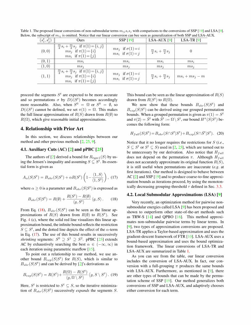
Table 1. The proposed linear conversions of non-submodular termsmijsisj with comparisons to the conversions of SSP [19] and LSA [9].Below, the subscript of mij is omitted. Notice that our linear conversion can bee seen as generalization of both SSP and LSA-AUX.

(sti, stj) Ours SSP [19] LSA-AUX [9] LSA-TR [9]

(0, 0)

m2 si + m

2 sj if π(1)=i, jmsj if π(1)=imsi if π(1)=j

msj if σ(1)= imsi if σ(1)=j

m2 si + m

2 sj 0

(0, 1) msi msi msi msi(1, 0) msj msj msj msj

(1, 1)

m2 si + m

2 sj if π(1)=i, jmsj if π(1)=imsi if π(1)=j

msj if σ(1)= imsi if σ(1)=j

m2 si + m

2 sj msi +msj −m

proceed the segments St are expected to be more accurateand so permutations σ by D(i|St) becomes accordinglymore reasonable. Also, when S0 = Ω or S0 = ∅, soD(i|St) cannot be defined, we set π(1) = Ω. This makesthe full linear approximations of R(S) drawn from R(∅) toR(Ω), which give reasonable initial approximations.

4. Relationship with Prior ArtIn this section, we discuss relationships between our

method and other previous methods [2, 25, 9].

4.1. Auxiliary Cuts (AC) [2] and pPBC [25]

The authors of [2] derived a bound for Rtype1(S) by us-ing the Jensen’s inequality and assuming S ⊆ St. Its essen-tial form is given as

Aα(S|St) = Bshr(S|St) + αR(St)

(1− 〈1, S〉〈1, St〉

), (17)

where α ≥ 0 is a parameter andBshr(S|St) is expressed as

Bshr(S|St) = R(∅) +R(St)−R(∅)〈g, St〉

〈g, S〉 . (18)

From Eq. (18), Bshr(S|St) can be seen as the linear ap-proximations of R(S) drawn from R(∅) to R(St). SeeFig. 4 (c), where the solid red line visualizes this linear ap-proximation bound, the infinite bound reflects the restrictionS ⊆ St, and the dotted line depicts the effect of the α-termin Eq. (17). The use of this bound results in successivelyshrinking segments: S0 ⊇ S1 ⊇ S2. pPBC [25] extendsAC by exhaustively searching the best α ∈ (−∞,∞) ineach iteration using parametric maxflow [15].

To point out a relationship to our method, we use an-other bound Bexp(S|St) for R(S), which is similar toBshr(S|St) and can be derived by [2]’s derivations as

Bexp(S|St) = R(St)+R(Ω)−R(St)

〈g,Ω \ St〉⟨g, S \ St

⟩. (19)

Here, St is restricted to St ⊆ S, so the iterative minimiza-tion of Bshr(S|St) successively expands the segments S.

This bound can be seen as the linear approximation ofR(S)drawn from R(St) to R(Ω).

We now show that these bounds Bshr(S|St) andBexp(S|St) can be derived using our grouped permutationbounds. When a grouped permutation is given as π(1) = St

and π(2) = St with St := Ω\St, our boundHπ(S|St) be-comes the following form:

Hfull(S|St)=Bshr(S∩St|St)+Bexp(S∩St|St). (20)

Notice that it no longer requires the restrictions for S (i.e.,S ⊆ St or St ⊆ S) used in [2, 25], which are turned out tobe unnecessary by our derivation. Also notice that Hfull

does not depend on the permutation π. Although Hfull

does not accurately approximate its original function R(S),it is still useful when permutations are inaccurate (e.g. atfirst iterations). Our method is designed to behave betweenAC [2] and SSP [19] and to produce coarse-to-fine approxi-mation bounds as iterations proceed, by using the monoton-ically decreasing grouping-threshold τ defined in Sec. 3.3.

4.2. Local Submodular Approximations (LSA) [9]

Very recently, an optimization method for pairwise non-submodular energies called LSA [9] has been proposed andshown to outperform other state-of-the-art methods suchas TRW-S [14] and QPBO [16]. This method approxi-mates non-submodular pairwise terms by linear terms. In[9], two types of approximation conversions are proposed.LSA-TR applies a Taylor-based approximation and uses thegradient-descent framework of FTR [10]. LSA-AUX uses abound-based approximation and uses the bound optimiza-tion framework. The linear conversions of LSA-TR andLSA-AUX are summarized in Table 1.

As you can see from the table, our linear conversionincludes the conversion of LSA-AUX. In fact, our con-version with a full-grouping π produces the same boundswith LSA-AUX. Furthermore, as mentioned in [9], thereare other types of bounds that can be made by the permu-tation scheme of SSP [19]. Our method generalizes bothconversions of SSP and LSA-AUX, and adaptively chooseseither conversion for each term.

5. ExperimentsFor evaluation, we use four variations of our method:

SDC-GEO is the proposed method described in Sec. 3.SDC-DIST uses the standard Euclidean distance for mak-ing permutations σ, but the other settings are the samewith SDC-GEO. SSP-DIST is SSP [19] that follows theimplementations by Rother et al. [22]. It is basically thesame with SDC-DIST but uses no mean approximations forbound constructions. We also use SSP-GEO, which is thesame with SSP-DIST but uses the geodesic distance. Notethat when S0 = Ω at the first iterations, we make permu-tations σ randomly for SSP-DIST and SSP-GEO, based on10× 10-pixels of patches as described in [22].

We also compare with three state-of-the-art methodsfor higher-order energies: AC [2] uses the bound Aα ofEq. (17). pPBC [25] uses the same bound but exhaus-tively chooses the best α using parametric maxflow [15].FTR [10] is the state-of-the-art of gradient-descent meth-ods. For pairwise energies, we compare with LSA-AUX,-TR [9] and pPBC-T,-B,-L [25] as state-of-the-art.

All the methods are implemented by C++, and run on asystem with a 3.5GHz Core i7 CPU and 16GB RAM.

5.1. Segmentation via Distribution Matching

Similarly to [25, 2, 22], we evaluate the performancesof the methods using the GrabCut dataset [23]. For pureevaluations of optimization performances, we learn the tar-get histograms from the ground truth1. We use a stan-dard 16-neighbor pairwise smoothness term similar to [23]:Q(S) = λ

∑ij max(wij , ε)|si − sj |/|pi − pj | where pi is

pixel coordinates and wij = exp(−β|Ii − Ij |2). Here, β isautomatically estimated as β = 2E[|Ii − Ij |2] the expecta-tion over all neighbor pairs. We use RGB-histograms.

Type-1: L2 and L1 Distance of Histograms

For Type-1 terms, we use the L2 and L1 distances betweenhistograms. For λ, ε, we use 1.0, 0.5 and 0.5, 0.5for the L2 and L1-distances, respectively. St is triviallyinitialized as S0 ← Ω. For both SDC-GEO and SDC-DIST,we use a grouping threshold τ = (µ+ 8s)/(t+ 1)2.5.

Tables 2 and 3 summarize the performance comparisons,showing average misclassified pixel rates, energy values ofE(S) and R(S), running times, and individual-image com-parisons with SDC-GEO. Among the seven methods, ourproposed method SDC-GEO outperforms the others for allerror and energy scores. In some cases, SDC-GEO com-pletely outperforms pPBC, AC, FTR, and SSP-DIST for allindividual images. Note that the error rates of SSP-DISTare better than the rates originally reported in [22] because

1If the target histograms are inaccurate, the minimum solutions ofE(S) are deviated from the ground truth [26], and the error rate criteriathus does not reflect the actual performances of the optimization methods.

Table 4. Evaluations on the GrabCut dataset [23] using the Bhat-tacharyya distance and KL divergence. We use 643 bins and thebounding box initialization.

MethodError (%) E(S) Time (sec)

Bhat. KL-div. Bhat. KL-div. Bhat. KL-div.SDC 0.373 0.515 -14906 7025 19.8 12.9

pPBC [25] 0.498 0.818 -14870 7057 1.8 1.5AC [2] 18.29 16.07 -11878 7490 0.4 0.4

FTR [10] 0.435 1.076 -14894 7049 2.9 6.4

the definition of pixel feature histograms is different2. Com-paring the results of SDC-DIST and SSP-DIST with L2 and643 bins, SDC-DIST finds more accurate segmentations inspite of the higher energies. This is because in SSP-DISTthe appearance consistencies are forced regardless of howpermutations σ and corresponding bounds are inaccurate,resulting in highly non-smooth, visibly bad local minimas.In Fig. 5, we show example results of L2 and L1 with 64bins. Figures 6 and 7 show the plots of the accuracy tran-sitions using the L2 and L1-distances w.r.t. the number ofbins. As shown, SDC-GEO is robust to the difference of thenumber of bins. In order to show robustness to initialization,we compare SDC-GEO, pPBC, and FTR using two types ofinitialization shown in Fig. 1. Unlike pPBC (and AC) thatcan only reduce the target regions, our method is robust toinitialization and finds very accurate solutions even for suchdifficult camouflage images.

Type-2: Bhattacharyya Distance and KL Divergence

We use Bhattacharyya distance and KL divergence asType-2. As described in Sec. 3.2, we use the pseudo boundoptimization scheme of [25] using parametric maxflow [15]for our method SDC-GEO. We show the performance com-parisons with pPBC, AC, and FTR in Table 4, where ourmethod outperforms the others in error and energy values. Itis worth noting that although SSP [19] is originally orientedfor supermodular functions, our extended method success-fully optimizes non-supermodular functions (Type-2).

5.2. Type-3: Image Deconvolution

We make a blurred image I by a mean filter and additiveGaussian noises: Ii = 1

9

∑j∈Wi

Ij+N (0, σ2), whereWi isa 3×3 window centered at i. We recover the original imageI by minimizing E(S) =

∑i∈Ω(Ii − 1

9

∑j∈Wi

sj)2. In

Fig. 8, we show example results of our method, pPBC [25],and LSA [9] for two noise levels σ = 0.15, 0.30. In Fig. 9,we show the plots of energies, squared errors (

∑i |si−Ii|2),

and running times. LSA-TR and pPBC-T,-L reach the lowerenergies but inaccurate results. Our method and LSA-AUXperform best in terms of both accuracy and efficiency.

2[22] uses a normalized 2D color vector and texton as a pixel feature,since the method is intended for co-segmentation and image retrieval.

Table 2. Evaluations on the GrabCut dataset [23] using L2-distance. We show average error rates, E(S), R(S), times over 50 images. Thelast column shows the number of images for which the proposed method (SDC-GEO) outperforms each method. We use 1923 and 643

bins.Method Error (%) E(S) R(S) Time (sec) SDC-GEO vs

(L2-distance) 1923 643 1923 643 1923 643 1923 643 1923 643

ref. Ground Truth 0 0 3569 3569 0 0 - - - -SDC-GEO 0.095 0.288 3511 3809 179 235 6.2 11.7 - -SDC-DIST 0.134 1.123 4121 18922 577 9946 2.3 2.7 32 46SSP-GEO 0.116 1.132 3594 6477 166 377 4.9 15.1 24 45

SSP-DIST [22] 0.312 2.575 4415 13969 295 877 2.0 4.2 32 50pPBC [25] 1.062 2.677 19381 190332 13187 176315 36.7 24.6 49 50

AC [2] 1.214 3.542 19888 195729 13646 177947 1.0 1.0 50 50FTR [10] 1.859 3.167 21003 153212 17669 146394 36.8 121.2 50 48

Table 3. Evaluations on the GrabCut dataset [23] using L1-distance. See Table 2 for the descriptions.Method Error (%) E(S) R(S) Time (sec) SDC-GEO vs

(L1-distance) 1923 643 1923 643 1923 643 1923 643 1923 643

ref. Ground Truth 0 0 1785 1785 0 0 - - - -SDC-GEO 0.033 0.205 1804 1882 54 120 5.4 9.4 - -SDC-DIST 0.041 0.242 1813 1967 70 229 1.9 3.8 38 42SSP-GEO 0.043 0.943 1813 2766 31 298 3.7 9.7 28 46

SSP-DIST [22] 0.075 1.341 1898 3666 50 411 1.6 2.4 34 48pPBC [25] 0.154 0.583 2013 2632 309 997 17.4 18.9 48 48

AC [2] 0.339 1.281 2502 4336 762 2476 0.6 0.6 50 50FTR [10] 0.147 0.366 1908 2105 277 495 46.1 100.7 46 41

Ground Truth SDC-GEO SSP-DIST [22] pPBC [25] AC [2] FTR [10]Figure 5. L2 (top) and L1 (bottom) examples. The segments are initialized as all foreground, and 643 bins of histograms are used.

0.0F

1.0F

2.0F

3.0F

4.0F

5.0F

32 64 96 128 160 192

Erro

rCR

ateC

(F)

NumberCofCBinsCperCChannel

SDC-GEO

pPBC

AC

FTR

Figure 6. Error rate transitions w.r.t. the number of bins (L2)

0.0F

0.5F

1.0F

1.5F

2.0F

2.5F

32 64 96 128 160 192

Erro

rCR

ateC

(F)

NumberCofCBinsCperCChannel

SDC-GEO

pPBC

AC

FTR

Figure 7. Error rate transitions w.r.t. the number of bins (L1)

Input SDC-GEO pPBC-T [25] pPBC-B [25] pPBC-L [25] LSA-AUX [10] LSA-TR [10]

Figure 8. Image deconvolution results for two images with noise levels of σ = 0.15 (top) and σ = 0.30 (bottom).

0

2

4

6

8

10

12

0.05 0.1 0.15 0.2 0.25 0.3

Ener

gyT(

10

e+2

)

NoiseTLevelTσ

SDC-GEO

pPBC-T

pPBC-B

pPBC-L

LSA-AUX

LSA-TR

SDC-GEO

PBC-BLSA-AUX

0

1

2

3

4

5

6

7

8

9

10

0.05 0.1 0.15 0.2 0.25 0.3

Squ

ared

PErr

orP

R10

e+2

)

NoisePLevelPσ

SDC-GEO

pPBC-T

pPBC-B

pPBC-L

LSA-AUX

LSA-TRSDC-GEO

PBC-BLSA-AUX

0.0

0.5

1.0

1.5

2.0

2.5

3.0

3.5

4.0

4.5

0.05 0.1 0.15 0.2 0.25 0.3

Tim

e (s

ec)

Noise Level σ

SDC-GEOpPBC-TpPBC-BpPBC-LLSA-AUXLSA-TR

Figure 9. Performance comparisons of image deconvolution. Convergence energies, square errors, and running times w.r.t. noise levels areshown. The values are averaged over 30 random noise images at each point. We use τ = (µ+s)/(t+1)2.5 for our method. Notice that ourmethod obtains more accurate solutions in spite of their higher energies, because our course-to-fine scheme avoids bad local minimums.

Input SDC-GEO LSA-AUX [9]

pPBC-T [25] pPBC-B [25] pPBC-L [25]Figure 10. Results of curvature optimization at the weight of 25.

5.4

5.5

5.6

5.7

5.8

5.9

6.0

6.1

6.2

6.3

6.4

19 20 21 22 23 24 25 26 27 28 29 30

Ener

gyWS

10

eX4

A

CurvatureWRegularizationWWeight

SDC-GEOpPBC-TpPBC-BpPBC-LLSA-AUXLSA-TR

Figure 11. Convergence energies w.r.t. curvature reg-ularization weights. We use τ = µ/(t+ 1)2.5.

5.3. Type-3: Curvature Regularization

We apply our method to a curvature regularization modelof [6] in image binarization. We show the input image andresults by our method, pPBC [25], and LSA [9] in Fig. 10.The plots in Fig. 11 show energies at convergence w.r.t. reg-ularization weights. Our method always reaches the lowestenergies and is most stable among all methods.

6. Conclusions

In this paper we have revisited SSP [19], an earlyapproach to higher-order energy optimization, and pro-

posed our method as generalization of SSP. The key ideaof our method is piecewise mean approximation bounds,which are designed to produce coarse-to-fine approximationbounds during iterations. We further show that our methodhas close connections to some state-of-the-art methods [2,25, 9]. Although the proposed method shows promising im-provements over state-of-the-art methods [25, 10, 9, 2], wewould like to further push the envelope by improving thedefinition of geodesic distance and the thresholding schemefor making grouped permutations.

AcknowledgmentsThe authors would thank to anonymous reviewers for

providing valuable feedbacks needed to improve this paper.This work was supported by JSPS KAKENHI Grant Num-ber 14J09001.

References[1] I. B. Ayed, H. M. Chen, K. Punithakumar, I. Ross, and S. Li.

Graph Cut Segmentation with a Global Constraint: Recov-ering Region Distribution via a Bound of the BhattacharyyaMeasure. In Proc. of IEEE Conf. on Computer Vision andPattern Recognition (CVPR), pages 3288–3295, 2010. 1, 2

[2] I. B. Ayed, L. Gorelick, and Y. Boykov. Auxiliary Cutsfor General Classes of Higher Order Functionals. In Proc.of IEEE Conf. on Computer Vision and Pattern Recognition(CVPR), pages 1304–1311, 2013. 1, 2, 3, 4, 5, 6, 7, 8

[3] Y. Boykov and M. P. Jolly. Interactive Graph Cuts for Op-timal Boundary & Region Segmentation of Objects in N-DImages. In Proc. of Int’l Conf. on Computer Vision (ICCV),pages 105–112, 2001. 1

[4] Y. Boykov and V. Kolmogorov. An Experimental Com-parison of Min-Cut/Max-Flow Algorithms for Energy Mini-mization in Vision. IEEE Trans. Pattern Anal. Mach. Intell.(TPAMI), 26:1124–1137, 2004. 1, 2, 4

[5] A. Criminisi, T. Sharp, and A. Blake. GeoS: Geodesic Im-age Segmentation. In Proc. of European Conf. on ComputerVision (ECCV), pages 99–112, 2008. 3, 4

[6] N. El-Zehiry and L. Grady. Fast Global Optimization of Cur-vature. In Proc. of IEEE Conf. on Computer Vision and Pat-tern Recognition (CVPR), pages 3257–3264, 2010. 1, 8

[7] S. Fujishige. Submodular Functions and Optimization, vol-ume 58. Elsevier Science, 2005. 2, 3

[8] S. Geman and D. Geman. Stochastic Relaxation, Gibbs Dis-tributions, and the Bayesian Restoration of Images. IEEETrans. Pattern Anal. Mach. Intell. (TPAMI), 6(6):721–741,1984. 1

[9] L. Gorelick, Y. Boykov, O. Veksler, I. Ben Ayed, and A. De-long. Submodularization for Binary Pairwise Energies. InProc. of IEEE Conf. on Computer Vision and Pattern Recog-nition (CVPR), 2014. 1, 2, 5, 6, 8

[10] L. Gorelick, F. R. Schmidt, and Y. Boykov. Fast Trust Re-gion for Segmentation. In Proc. of IEEE Conf. on ComputerVision and Pattern Recognition (CVPR), pages 1714–1721,2013. 1, 2, 5, 6, 7, 8

[11] L. Gorelick, F. R. Schmidt, Y. Boykov, A. Delong, and A. D.Ward. Segmentation with Non-Linear Regional Constraintsvia Line-Search Cuts. In Proc. of European Conf. on Com-puter Vision (ECCV), pages 583–0597, 2012. 1, 2

[12] R. Iyer, S. Jegelka, and J. Bilmes. Fast Semidifferential-based Submodular Function Optimization. Proc. of Interna-tional Conference on Machine Learning (ICML), 28(3):855–863, 2013. 2

[13] H. Jiang. Linear Solution to Scale Invariant Global FigureGround Separation. In Proc. of IEEE Conf. on Computer Vi-sion and Pattern Recognition (CVPR), pages 678–685, 2012.2

[14] V. Kolmogorov. Convergent Tree-Reweighted MessagePassing for Energy Minimization. IEEE Trans. Pattern Anal.Mach. Intell. (TPAMI), 28(10):1568–1583, 2006. 5

[15] V. Kolmogorov, Y. Boykov, and C. Rother. Applications ofParametric Maxflow in Computer Vision. In Proc. of Int’lConf. on Computer Vision (ICCV), 2007. 4, 5, 6

[16] V. Kolmogorov and C. Rother. Minimizing NonsubmodularFunctions with Graph Cuts – A Review. IEEE Trans. PatternAnal. Mach. Intell. (TPAMI), 29(7):1274–1279, 2007. 2, 5

[17] V. Kolmogorov and R. Zabin. What Energy Functions CanBe Minimized via Graph Cuts? IEEE Trans. Pattern Anal.Mach. Intell. (TPAMI), 26(2):147–159, 2004. 1, 2

[18] L. Mukherjee, V. Singh, and C. Dyer. Half-Integrality basedAlgorithms for Cosegmentation of Images. In Proc. of IEEEConf. on Computer Vision and Pattern Recognition (CVPR),pages 2028–2035, 2009. 2

[19] M. Narasimhan and J. A. Bilmes. A Submodular-Supermodular Procedure with Applications to Discrimina-tive Structure Learning. In Proc. of Conf. on Uncertainty inArtificial Intelligence (UAI), pages 404–412, 2005. 1, 2, 3,5, 6, 8

[20] V.-Q. Pham, K. Takahashi, and T. Naemura. Foreground-Background Segmentation using Iterated DistributionMatching. In Proc. of IEEE Conf. on Computer Vision andPattern Recognition (CVPR), pages 2113–2120, 2011. 1

[21] B. L. Price, B. Morse, and S. Cohen. Geodesic Graph Cutfor Interactive Image Segmentation. In Proc. of IEEE Conf.on Computer Vision and Pattern Recognition (CVPR), pages3288–3295, 2010. 1

[22] C. Rother, V. Kolmogorov, T. Minka, and A. Blake.Cosegmentation of Image Pairs by Histogram Matching–Incorporating a Global Constraint into MRFs. In Proc. ofIEEE Conf. on Computer Vision and Pattern Recognition(CVPR), pages 993–100, 2006. 1, 2, 4, 6, 7

[23] C. Rother, V. Kolmogorv, and A. Blake. GrabCut: InteractiveForeground Extraction Using Iterated Graph Cuts. Proc. ofSIGGRAPH (ACM Trans. on Graph.), 23:309–314, 2004. 1,6, 7

[24] A. Schrijver. A Combinatorial Algorithm Minimizing Sub-modular Functions in Strongly Polynomial Time. J. of Com-binational Theory Ser. B, 80(2):346–355, 2000. 2

[25] M. Tang, I. Ben Ayed, and Y. Boykov. Pseudo-Bound Opti-mization for Binary Energies. In Proc. of European Conf. onComputer Vision (ECCV), pages 691–707, 2014. 1, 2, 4, 5,6, 7, 8

[26] T. Taniai, V.-Q. Pham, K. Takahashi, and T. Naemura. ImageSegmentation using Dual Distribution Matching. In Proc.of British Machine Vision Conf. (BMVC), pages 74.1–74.11,2012. 1, 6

[27] P. J. Toivanen. New Geodesic Distance Transforms for Gray-scale Images. Pattern Recogn. Lett., 17(5):437–450, 1996. 4

[28] S. Vicente, V. Kolmogorov, and C. Rother. CosegmentationRevisited: Models and Optimization. In Proc. of EuropeanConf. on Computer Vision (ECCV), pages 465–479, 2010. 2