Embed Size (px)
Citation preview
arX
iv:1
609.
0456
5v2
[he
p-th
] 2
0 Ju
l 201
7Preprint number: KIAS-P16067, KOBE-TH-16-06
Supersymmetry in the 6D Dirac action
Yukihiro Fujimoto1, Kouhei Hasegawa2, Kenji Nishiwaki3, Makoto
Sakamoto4, and Kentaro Tatsumi5
1National Institute of Technology, Oita College, Oita 870-0152, Japan
∗E-mail: [email protected]
2Department of Physics, Kobe University, Kobe 657-8501, Japan
∗E-mail: [email protected]
3School of Physics, Korea Institute for Advanced Study, Seoul 02455,
Republic of Korea
∗E-mail: [email protected]
4Department of Physics, Kobe University, Kobe 657-8501, Japan
∗E-mail: [email protected]
5Department of Physics, Kobe University, Kobe 657-8501, Japan
∗E-mail: [email protected]
. . . . . . . . . . . . . . . . . . . . . . . . . . . . . . . . . . . . . . . . . . . . . . . . . . . . . . . . . . . . . . . . . . . . . . . . . . . . . . . .We investigate a 6d Dirac fermion on a rectangle. It is found that the 4d spectrum is governedby N = 2 supersymmetric quantum mechanics. Then we demonstrate that the supersymmetryis very useful for classifying all the allowed boundary conditions and to expand the 6d Diracfield in Kaluza–Klein modes. A striking feature of the model is that even though the 6d Diracfermion has non-vanishing bulk mass, the 4d mass spectrum can contain degenerate masslesschiral fermions, which may provide a hint to solve the problem of the generation of quarksand leptons. It is pointed out that zero-energy solutions are not affected by the presence ofthe boundaries, while the boundary conditions work well for determining the positive-energysolutions. We also provide a brief discussion on possible boundary conditions in the generalcase, especially those on polygons.. . . . . . . . . . . . . . . . . . . . . . . . . . . . . . . . . . . . . . . . . . . . . . . . . . . . . . . . . . . . . . . . . . . . . . . . . . . . . . . . . . . . . . . . . . . . . . . . . . . . .
Subject Index B15, B33
1 typeset using PTPTEX.cls
1 Introduction
The standard model has been completely established by the discovery of the Higgs boson
[1, 2], and describes well the low-energy physics below the weak scale. Despite the great
success of the standard model, it will be natural to regard the standard model as a low-
energy effective theory of some more fundamental theories defined at higher energy scales.
This is because the standard model leaves various problems to be solved.
Promising candidates beyond the standard model are the models on higher-dimensional
space-times with compact extra dimensions. These models could solve the generation problem
[3–9] and the fermion mass hierarchy one [10–16], and naturally explain the quark and
lepton flavor structure [17–20] of the standard model. Many proposals have been made to
explain the quark and lepton mass hierarchies and their flavor structures naturally from an
extra-dimensional point of view.
Although extra-dimensional models will be expected to solve the generation problem,
phenomenologically realistic models that solve the problem are very limited. A possible
mechanism for producing degenerate massless chiral fermions is to put extra dimensions in
a homogeneous magnetic field [18, 20–29]. Another mechanism is to put point interactions
on an extra dimension [30–33]. It would be desirable to find new mechanism that solves the
above problems of the standard model and that can lead to phenomenologically realistic
models with a simple setup.
In the context of a five-dimensional (5d) gauge theory, it has been shown that a 4d mass-
less chiral fermion appears from a 5d Dirac fermion with a suitable boundary condition (see
e.g. [34]). Furthermore, the 5d Dirac mass term plays an important role in the localization of
zero-mode functions. Thereby, it can become a source of the observed fermion mass hierar-
chy. Unfortunately, however, in the case of 5d, only one 4d chiral fermion appears from a 5d
Dirac field. On the other hand, it would be expected that several 4d massless chiral fermions
may emerge in the case of a higher-dimensional Dirac fermion more than 5d that contains
more degrees of freedom than those in 5d. Our goal is to solve the generation problem as
well as other problems in the standard model from a higher-dimensional Dirac action point
of view.
In Ref. [35], the 4d mass spectrum of a 6d Dirac fermion was investigated. An interesting
observation is that two 4d massless chiral fermions can appear, even though the 6d Dirac
action contains a non-zero bulk massM . The results strongly suggest that higher-dimensional
Dirac fermions can provide more than two 4d massless chiral fermions and could solve the
generation problem. Unfortunately, it is not straightforward to extend the analysis given in
Ref. [35] to the higher-dimensional Dirac action, because the origin of the degeneracy of the
2
4d mass spectrum (four for the massive modes, and two for the massless modes) has been
obscure, and it is especially unclear how to expand Dirac fields into Kaluza–Klein modes for
general higher dimensions.
In this paper, we revisit the 6d Dirac fermion and reveal hidden structures in the 4d mass
spectrum from a symmetry point of view, in great detail. We show that the 4d mass spectrum
is governed by an N = 2 quantum-mechanical supersymmetry, and the degeneracy of the
4d mass spectrum can be explained by the supersymmetry (with an additional symmetry of
the action). This supersymmetric structure makes it clear why the 4d massless zero modes
become chiral. This is because 4d massive modes always form supermultiplets and then
become Dirac fermions, but each massless zero mode does not form a supermultiplet and
hence has no chiral partner to form a Dirac fermion. We further find that the supersymmetry
is very powerful for analyzing the Kaluza–Klein mode expansions and determining the class of
allowed boundary conditions on extra dimensions. We expect that our analysis can apply for
general higher-dimensional Dirac fermions and hence hope to answer the question of whether
or not Dirac fermions with more than two extra dimensions can solve the generation and
fermion mass hierarchy problems.
It is interesting to note that the supersymmetric structure is a common feature in extra
dimensions. This is because similar supersymmetric structures have been found in higher-
dimensional gauge and gravity theories [36–43] (see also [44, 45]). Thus, it would be of great
interest to understand the role of the supersymmetry in extra dimensions thoroughly.
This paper is organized as follows. We first give the setup of our model in Section 2 and
then show, in Section 3, that N = 2 supersymmetric quantum mechanics is hidden in the 6d
Dirac equation. In Section 4, we classify the allowed boundary conditions with the help of the
supersymmetry. In Sections 5 and 6, we explicitly construct positive-energy eigenfunctions
and point out a problem in determining zero-energy solutions. The degeneracy of positive-
energy states are explained from symmetry transformations in Section 7. In section 8, we
provide a brief discussion on possible boundary conditions in the general case, especially
those on polygons. Section 9 is devoted to conclusions and discussions.
2 Six-dimensional Dirac fermion on a rectangle
Let us start with the 6d Dirac action
S =
∫d4x
∫ L1
0dy1
∫ L2
0dy2Ψ(x, y)
[iΓA∂A −M
]Ψ(x, y), (2.1)
where Ψ(x, y) is an eight-component Dirac spinor in six dimensions and M is the bulk mass
of the Dirac fermion. The 6d space-time is taken to be the direct product of the 4d Minkowski
3
space-time and the 2d rectangle. The coordinates of the 4d Minkowski space-time and the
2d rectangle are denoted by xµ (µ = 0, 1, 2, 3) and yj (j = 1, 2), respectively. The domain of
the rectangle is set as 0 ≤ y1 ≤ L1 and 0 ≤ y2 ≤ L2.
The Dirac action (2.1) leads to the Dirac equation
[iΓµ∂µ + iΓy1∂y1 + iΓy2∂y2 −M
]Ψ(x, y) = 0. (2.2)
The 6d gamma matrices ΓA (A = 0, 1, 2, 3, y1, y2) are required to satisfy
{ΓA,ΓB} = −2ηAB I8, (A,B = 0, 1, 2, 3, y1, y2),
(ΓA)† =
{+ΓA A = 0,
−ΓA A 6= 0,(2.3)
with the 6d metric diag ηAB = (−1, 1, 1, 1, 1, 1). Here, In denotes the n× n identity matrix.
The Dirac conjugate Ψ is defined by Ψ = Ψ†Γ0, as usual.
In order to extract a quantum-mechanical supersymmetric structure from the Dirac
equation (2.2), it may be necessary to drive the equation without including the gamma
matrices Γy1 and Γy2. For this purpose, it turns out to be convenient to introduce the
matrices Γ5 and Γy such as
Γ5 ≡ iΓ0Γ1Γ2Γ3, (2.4)
Γy ≡ iΓy1Γy2, (2.5)
where Γy is an analogue of γ5 in the extra dimensions.
Since Γy commutes with Γ5, we can introduce simultaneous eigenstates of Γ5 and Γy
defined by
Γ5ΨR± = +ΨR±, Γ5ΨL± = −ΨL±, (2.6)
ΓyΨR± = ±ΨR±, ΓyΨL± = ±ΨL±. (2.7)
By use of the projection matrices, ΨR± and ΨL± can be constructed from Ψ as
ΨR± ≡ PRP±Ψ, ΨL± ≡ PLP±Ψ, (2.8)
where
PR =1
2(I8 + Γ5), PL =
1
2(I8 − Γ5), (2.9)
P± =1
2(I8 ± Γy). (2.10)
4
In terms of the eigenstates of Γ5 and Γy, the Dirac equation (2.2) can be decomposed as
iΓµ∂µΨR+ = −iΓy1(∂y1 − i∂y2)ΨL− +MΨL+,
iΓµ∂µΨR− = −iΓy1(∂y1 + i∂y2)ΨL+ +MΨL−,
iΓµ∂µΨL+ = −iΓy1(∂y1 − i∂y2)ΨR− +MΨR+,
iΓµ∂µΨL− = −iΓy1(∂y1 + i∂y2)ΨR+ +MΨR−. (2.11)
Furthermore, in order to remove iΓy1 from the above equations, we may redefine the fields
ΨR± and ΨL± as
ΨR1 ≡ ΨR+, ΨR2 ≡ iΓy1ΨR−,
ΨL1 ≡ ΨL+, ΨL2 ≡ iΓy1ΨL−. (2.12)
Then, we have succeeded in eliminating the gamma matrix Γy1 from (2.11) and in rewriting
(2.11) into the form
iΓµ∂µ
ΨR1(x, y)
ΨR2(x, y)
ΨL1(x, y)
ΨL2(x, y)
= (Q⊗ I2)
ΨR1(x, y)
ΨR2(x, y)
ΨL1(x, y)
ΨL2(x, y)
, (2.13)
where I2 acts on two-dimensional spinors ΨR1, ΨR2, ΨL1, ΨL2, and the 4× 4 matrix Q is
defined by
Q ≡
0 0 M −(∂y1 − i∂y2)0 0 ∂y1 + i∂y2 −MM −(∂y1 − i∂y2) 0 0
∂y1 + i∂y2 −M 0 0
. (2.14)
It should be emphasized that Q does not act on spinor indices but on the “flavor” space
displayed in (2.13) and satisfies the relation
Q2 =[−∂2y1 − ∂
2y2 +M2
]I4. (2.15)
Thus, the differential operator Q2 turns out to correspond to a Laplacian on the extra
dimensions.
In the following sections, we will show that Q can be regarded as a supercharge of N = 2
supersymmetric quantum mechanics and that the 4d mass spectrum of the 6d Dirac fermion
system is governed by the supersymmetry.
5
3 Hidden N = 2 supersymmetry
Since we would like to regard Q as a supercharge in supersymmetric quantum mechanics,
we may introduce a Hamiltonian H by
H = Q2. (3.1)
In order for the system to be supersymmetric, we further need to introduce the “fermion”
number operator F which should satisfy the relation [46]
(−1)FQ = −Q(−1)F ,[(−1)F
]2= I4. (3.2)
Then, the operator H , Q and (−1)F are assumed to act on four-component wavefunctions
Φ(y) =
f1(y)
f2(y)
g1(y)
g2(y)
(3.3)
that depend only on y1 and y2.
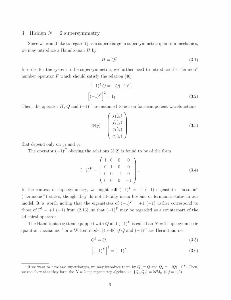
The operator (−1)F obeying the relations (3.2) is found to be of the form
(−1)F =
1 0 0 0
0 1 0 0
0 0 −1 0
0 0 0 −1
. (3.4)
In the context of supersymmetry, we might call (−1)F = +1 (−1) eigenstates “bosonic”
(“fermionic”) states, though they do not literally mean bosonic or fermionic states in our
model. It is worth noting that the eigenstates of (−1)F = +1 (−1) rather correspond to
those of Γ5 = +1 (−1) from (2.13), so that (−1)F may be regarded as a counterpart of the
4d chiral operator.
The Hamiltonian system equipped with Q and (−1)F is called an N = 2 supersymmetric
quantum mechanics 1 or a Witten model [46–48] if Q and (−1)F are Hermitian, i.e.
Q† = Q, (3.5)[(−1)F
]†= (−1)F . (3.6)
1 If we want to have two supercharges, we may introduce them by Q1 ≡ Q and Q2 ≡ −iQ(−1)F . Then,we can show that they form the N = 2 supersymmetry algebra, i.e. {Qi, Qj} = 2Hδij (i, j = 1, 2).
6
It should be emphasized that the above Hermiticity property of Q is not trivial because
the extra dimensions have boundaries. In fact, we will see in the next section that the Her-
miticity requirement (3.5) and the compatibility condition with (−1)F severely restrict the
allowed boundary conditions for the wavefunctions (3.3) at the boundaries of the rectangle.
4 Classification of allowed boundary conditions
4.1 Requirement of Hermiticity for Q
Since we have taken the extra dimensions to be a rectangle, the requirement for Her-
miticity for the supercharge Q is not trivial. In fact, we will see below that the Hermiticity
requirement severely restricts the class of allowed boundary conditions for Φ(y) at y1 = 0, L1
and y2 = 0, L2.
To be more precise, we require that the supercharge Q is Hermitian under the inner
product
〈Φ′,Φ〉 ≡∫ L1
0dy1
∫ L2
0dy2
(Φ′(y)
)†Φ(y)
=
∫ L1
0dy1
∫ L2
0dy2
{(f ′1(y)
)∗f1(y) +
(f ′2(y)
)∗f2(y) +
(g′1(y)
)∗g1(y) +
(g′2(y)
)∗g2(y)
},
(4.1)
where
Φ(y) =
f1(y)
f2(y)
g1(y)
g2(y)
, Φ′(y) =
f ′1(y)
f ′2(y)
g′1(y)
g′2(y)
. (4.2)
Then, in order for Q to be Hermitian, Q has to satisfy
〈QΦ′,Φ〉 = 〈Φ′, QΦ〉 (4.3)
for arbitrary four-component wavefunctions Φ(y) and Φ′(y) with appropriate boundary
conditions.
To make our analysis tractable, we assume that the probability current in the directions
of the extra dimensions terminates at each point of the boundaries of the rectangle. Then,
7

(4.3) turns out to reduce to the conditions
(f ′1(y)
)∗g2(y)−
(f ′2(y)
)∗g1(y) +
(g′1(y)
)∗f2(y)−
(g′2(y)
)∗f1(y) = 0 at y1 = 0, L1,
(4.4)(f ′1(y)
)∗g2(y) +
(f ′2(y)
)∗g1(y) +
(g′1(y)
)∗f2(y) +
(g′2(y)
)∗f1(y) = 0 at y2 = 0, L2,
(4.5)
4.2 Allowed boundary conditions in the y1-direction
Let us first investigate condition (4.4). To solve condition (4.4), we first restrict our
considerations to the case of Φ′(y) = Φ(y), i.e. f ′j(y) = fj(y) and g′j(y) = gj(y) (j = 1, 2).
This restriction would give a necessary condition for (4.4). We will, however, verify that the
derived boundary conditions are sufficient as well as necessary.
For f ′j(y) = fj(y) and g′j(y) = gj(y) (j = 1, 2), condition (4.4) can be written in the form
ρ1(y)†λ1(y) + λ1(y)
†ρ1(y) = 0 at y1 = 0, L1, (4.6)
where ρ1(y) and λ1(y) are two-component vectors defined by
ρ1(y) =
(f1(y)
f2(y)
), λ1(y) = i
(−g2(y)g1(y)
). (4.7)
A crucial observation is that the condition (4.6) can be rewritten as
|ρ1(y) + L0λ1(y)|2 = |ρ1(y)− L0λ1(y)|2 at y1 = 0, L1, (4.8)
where L0 is a non-zero real constant whose value is irrelevant unless L0 is non-vanishing.
General solutions to (4.8) are easily found in the form
ρ1(y) + L0λ1(y) = U1
(ρ1(y)− L0λ1(y)
)at y1 = 0, L1,
or equivalently
(I2 − U1
)ρ1(y) = −L0
(I2 + U1
)λ1(y) at y1 = 0, L1, (4.9)
where U1 is an arbitrary 2× 2 unitary matrix.
We have required the Hermiticity of the supercharge Q in order for the system to be
supersymmetric. The Hermiticity of Q is, however, not enough to preserve the supersymme-
try. We should further require that the boundary conditions are compatible with the fermion
number operator (−1)F .
8
Since (−1)F commutes with the Hamiltonian H , (−1)F can be regarded as a conserved
charge. Hence, the eigenvalues of (−1)F should be conserved, otherwise the supersymmetric
structure would be destroyed. Since ρ1(y) =(f1(y), f2(y)
)Tand λ1(y) =
(−g2(y), g1(y)
)T
correspond to (−1)F = +1 and −1, respectively, ρ1(y) should not be related to λ1(y) at the
boundaries in order for eigenvalues of (−1)F to be conserved.2 Therefore, the condition (4.9)
has to reduce to
(I2 − U1
)ρ1(y) = 0, at y1 = 0, L1, (4.10)
(I2 + U1
)λ1(y) = 0, at y1 = 0, L1. (4.11)
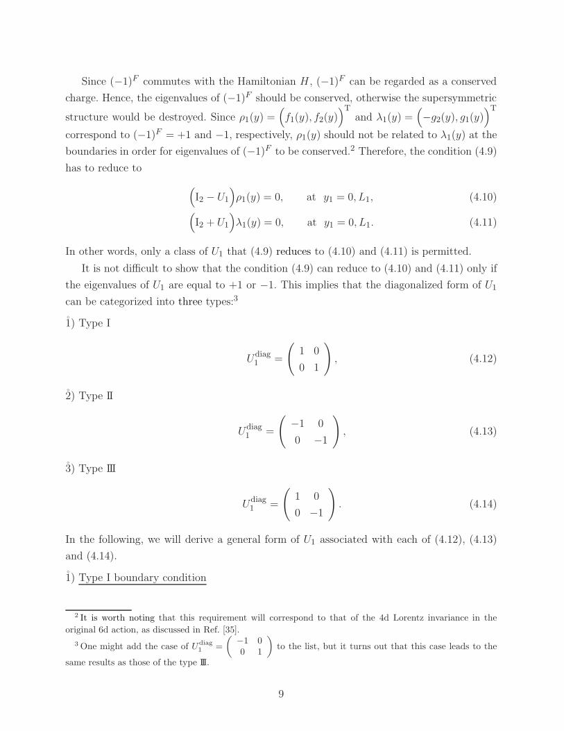
In other words, only a class of U1 that (4.9) reduces to (4.10) and (4.11) is permitted.
It is not difficult to show that the condition (4.9) can reduce to (4.10) and (4.11) only if
the eigenvalues of U1 are equal to +1 or −1. This implies that the diagonalized form of U1
can be categorized into three types:3
1) Type I
Udiag1 =
(1 0
0 1
), (4.12)
2) Type II
Udiag1 =
(−1 0
0 −1
), (4.13)
3) Type III
Udiag1 =
(1 0
0 −1
). (4.14)
In the following, we will derive a general form of U1 associated with each of (4.12), (4.13)
and (4.14).
1) Type I boundary condition
2 It is worth noting that this requirement will correspond to that of the 4d Lorentz invariance in the
original 6d action, as discussed in Ref. [35].
3 One might add the case of Udiag1 =
(−1 00 1
)to the list, but it turns out that this case leads to the
same results as those of the type III.
9
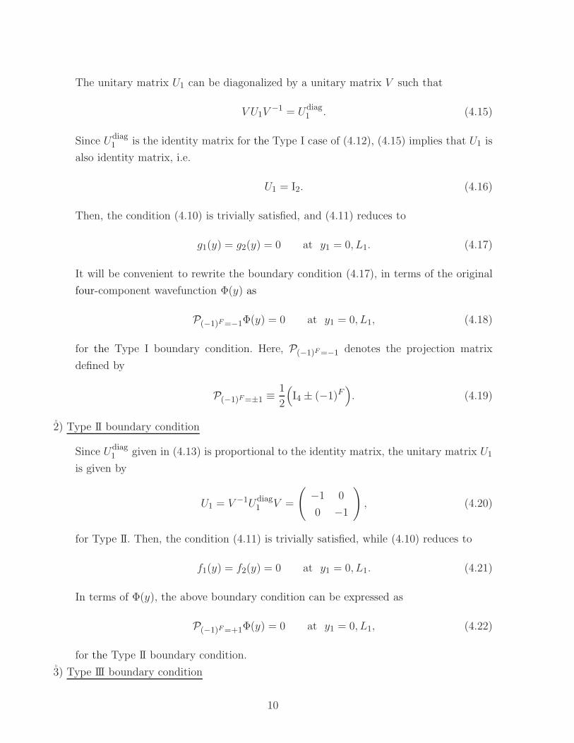
The unitary matrix U1 can be diagonalized by a unitary matrix V such that
V U1V−1 = Udiag
1 . (4.15)
Since Udiag1 is the identity matrix for the Type I case of (4.12), (4.15) implies that U1 is
also identity matrix, i.e.
U1 = I2. (4.16)
Then, the condition (4.10) is trivially satisfied, and (4.11) reduces to
g1(y) = g2(y) = 0 at y1 = 0, L1. (4.17)
It will be convenient to rewrite the boundary condition (4.17), in terms of the original
four-component wavefunction Φ(y) as
P(−1)F=−1Φ(y) = 0 at y1 = 0, L1, (4.18)
for the Type I boundary condition. Here, P(−1)F=−1 denotes the projection matrix
defined by
P(−1)F=±1 ≡1
2
(I4 ± (−1)F
). (4.19)
2) Type II boundary condition
Since Udiag1 given in (4.13) is proportional to the identity matrix, the unitary matrix U1
is given by
U1 = V −1Udiag1 V =
(−1 0
0 −1
), (4.20)
for Type II. Then, the condition (4.11) is trivially satisfied, while (4.10) reduces to
f1(y) = f2(y) = 0 at y1 = 0, L1. (4.21)
In terms of Φ(y), the above boundary condition can be expressed as
P(−1)F=+1Φ(y) = 0 at y1 = 0, L1, (4.22)
for the Type II boundary condition.
3) Type III boundary condition
10
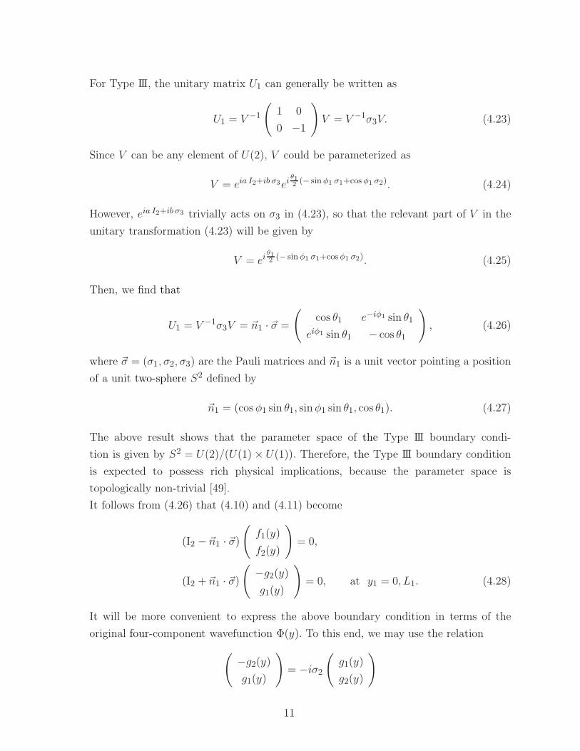
For Type III, the unitary matrix U1 can generally be written as
U1 = V −1
(1 0
0 −1
)V = V −1σ3V. (4.23)
Since V can be any element of U(2), V could be parameterized as
V = eia I2+ib σ3eiθ12 (− sinφ1 σ1+cos φ1 σ2). (4.24)
However, eia I2+ib σ3 trivially acts on σ3 in (4.23), so that the relevant part of V in the
unitary transformation (4.23) will be given by
V = eiθ12 (− sinφ1 σ1+cosφ1 σ2). (4.25)
Then, we find that
U1 = V −1σ3V = ~n1 · ~σ =
(cos θ1 e−iφ1 sin θ1
eiφ1 sin θ1 − cos θ1
), (4.26)
where ~σ = (σ1, σ2, σ3) are the Pauli matrices and ~n1 is a unit vector pointing a position
of a unit two-sphere S2 defined by
~n1 = (cos φ1 sin θ1, sinφ1 sin θ1, cos θ1). (4.27)
The above result shows that the parameter space of the Type III boundary condi-
tion is given by S2 = U(2)/(U(1)× U(1)). Therefore, the Type III boundary condition
is expected to possess rich physical implications, because the parameter space is
topologically non-trivial [49].
It follows from (4.26) that (4.10) and (4.11) become
(I2 − ~n1 · ~σ)(f1(y)
f2(y)
)= 0,
(I2 + ~n1 · ~σ)(−g2(y)g1(y)
)= 0, at y1 = 0, L1. (4.28)
It will be more convenient to express the above boundary condition in terms of the
original four-component wavefunction Φ(y). To this end, we may use the relation
(−g2(y)g1(y)
)= −iσ2
(g1(y)
g2(y)
)
11
and combine the two conditions of (4.28) into a single one as
P~n1·~Σ1=−1
Φ(y) = 0 at y1 = 0, L1, (4.29)
where P~n1·~Σ1=−1
is defined by
P~n1·~Σ1=±1
≡ 1
2
(I4 ± ~n1 · ~Σ1
), (4.30)
~Σ1 ≡(~σ 0
0 −σ2~σσ2
). (4.31)
Since (~n1 · ~Σ1)2 = I4 with ~n1 · ~n1 = 1, P
~n1·~Σ1=−1can be regarded as the projection
matrix on a subspace of ~n1 · ~Σ1 = −1.It is interesting to note that every boundary condition of Type I, II, and III can be
expressed by use of the projection matrices, P(−1)F=−1, P(−1)F=+1 and P~n·~Σ1=−1
, respec-
tively, and that those representations become important in the subsection 4.4 to verify the
sufficiency of the conditions obtained above.
4.3 Allowed boundary conditions in the y2-direction
Let us next investigate the condition (4.5), whose solutions will give possible boundary
conditions in the y2-direction. As before, by taking Φ′(y) = Φ(y), (4.5) is found to be written
as
|ρ2(y) + L0λ2(y)|2 = |ρ2(y)− L0λ2(y)|2 at y2 = 0, L2, (4.32)
where
ρ2(y) =
(f1(y)
f2(y)
), λ2(y) =
(g2(y)
g1(y)
). (4.33)
Here, L0 is a non-zero real constant whose value is irrelevant unless L0 is non-vanishing.
General solutions to (4.32) are given by(I2 − U2
)ρ2(y) = −L0
(I2 + U2
)λ2(y) at y2 = 0, L2, (4.34)
where U2 is an arbitrary 2× 2 unitary matrix.
Requiring that the boundary conditions have to be compatible with the eigenvalues of
(−1)F , we find that (4.34) should reduce to(I2 − U2
)ρ2(y) = 0, (4.35)
(I2 + U2
)λ2(y) = 0 at y2 = 0, L2. (4.36)
This implies that the eigenvalues of U2 have to be +1 or −1. As before, we can then show
that the form of U2 is classified into three categories such as
12
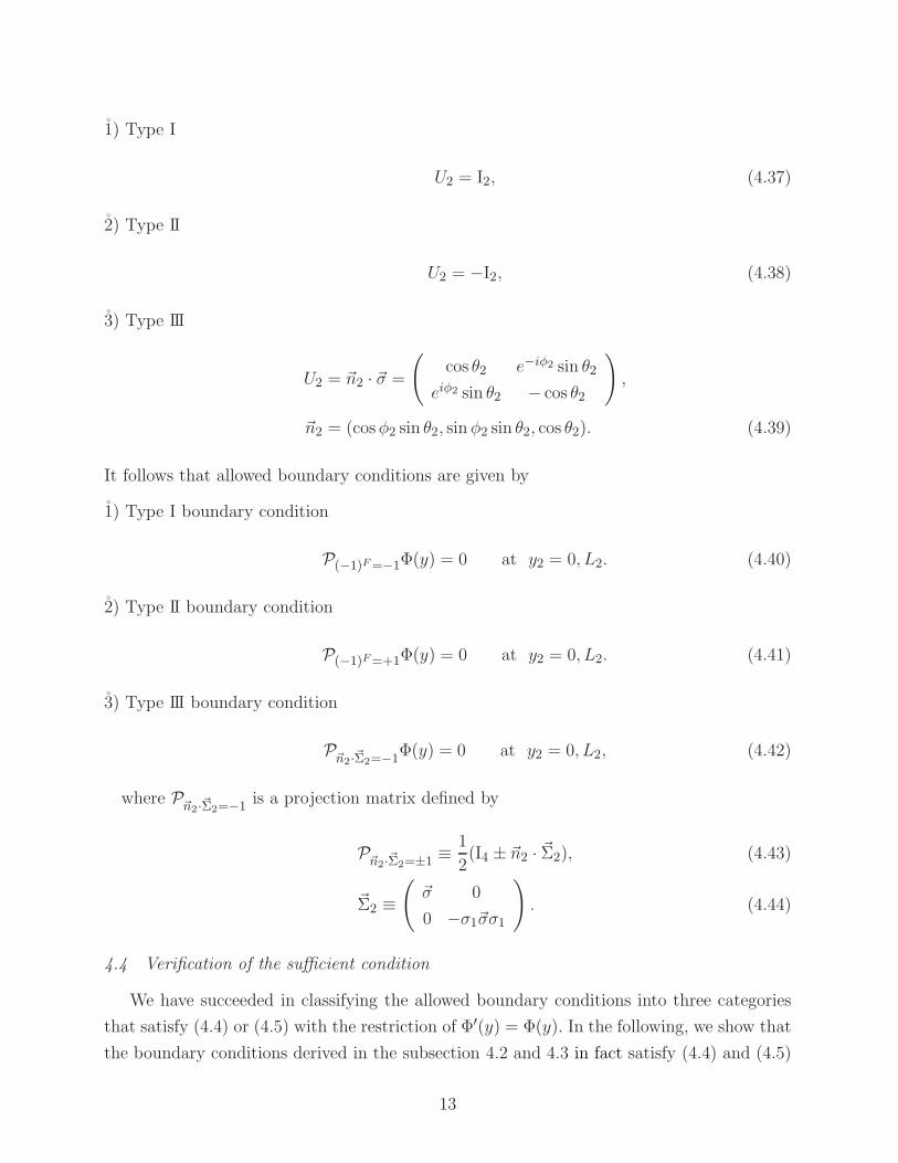
1) Type I
U2 = I2, (4.37)
2) Type II
U2 = −I2, (4.38)
3) Type III
U2 = ~n2 · ~σ =
(cos θ2 e−iφ2 sin θ2
eiφ2 sin θ2 − cos θ2
),
~n2 = (cosφ2 sin θ2, sinφ2 sin θ2, cos θ2). (4.39)
It follows that allowed boundary conditions are given by
1) Type I boundary condition
P(−1)F=−1Φ(y) = 0 at y2 = 0, L2. (4.40)
2) Type II boundary condition
P(−1)F=+1Φ(y) = 0 at y2 = 0, L2. (4.41)
3) Type III boundary condition
P~n2·~Σ2=−1
Φ(y) = 0 at y2 = 0, L2, (4.42)
where P~n2·~Σ2=−1
is a projection matrix defined by
P~n2·~Σ2=±1
≡ 1
2(I4 ± ~n2 · ~Σ2), (4.43)
~Σ2 ≡(~σ 0
0 −σ1~σσ1
). (4.44)
4.4 Verification of the sufficient condition
We have succeeded in classifying the allowed boundary conditions into three categories
that satisfy (4.4) or (4.5) with the restriction of Φ′(y) = Φ(y). In the following, we show that
the boundary conditions derived in the subsection 4.2 and 4.3 in fact satisfy (4.4) and (4.5)
13
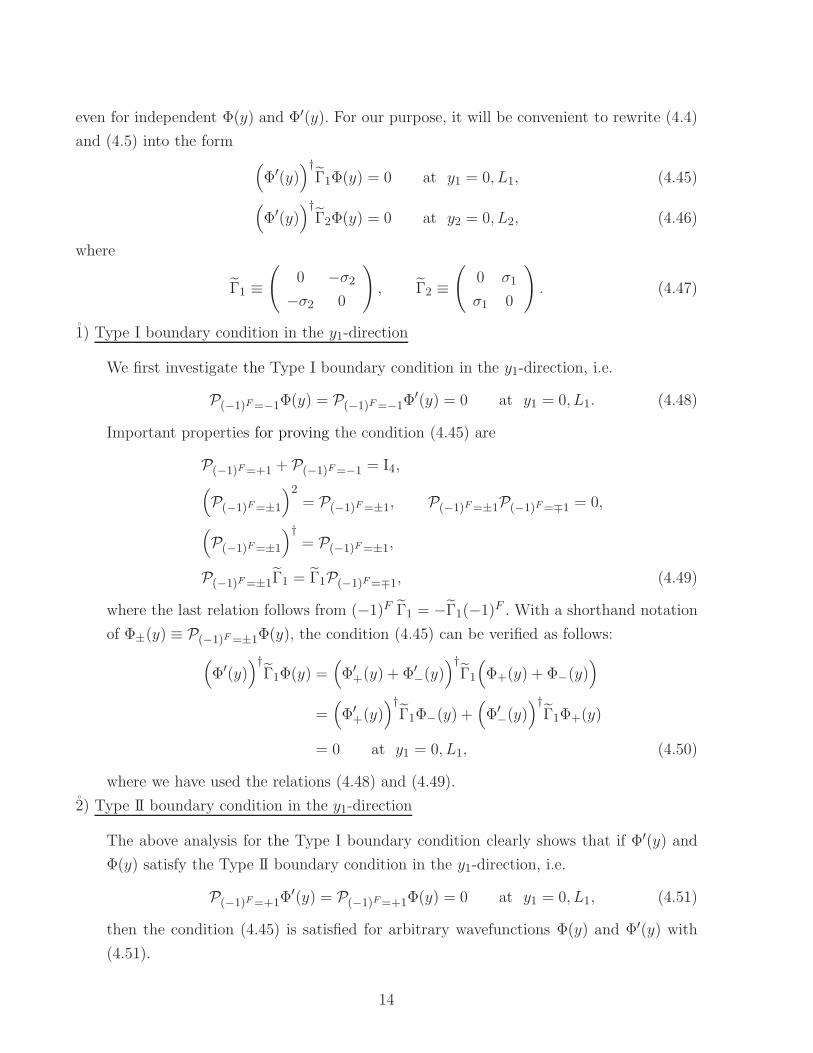
even for independent Φ(y) and Φ′(y). For our purpose, it will be convenient to rewrite (4.4)
and (4.5) into the form(Φ′(y)
)†Γ1Φ(y) = 0 at y1 = 0, L1, (4.45)
(Φ′(y)
)†Γ2Φ(y) = 0 at y2 = 0, L2, (4.46)
where
Γ1 ≡(
0 −σ2−σ2 0
), Γ2 ≡
(0 σ1
σ1 0
). (4.47)
1) Type I boundary condition in the y1-direction
We first investigate the Type I boundary condition in the y1-direction, i.e.
P(−1)F=−1Φ(y) = P(−1)F=−1Φ′(y) = 0 at y1 = 0, L1. (4.48)
Important properties for proving the condition (4.45) are
P(−1)F=+1 + P(−1)F=−1 = I4,(P(−1)F=±1
)2= P(−1)F=±1, P(−1)F=±1P(−1)F=∓1 = 0,
(P(−1)F=±1
)†= P(−1)F=±1,
P(−1)F=±1Γ1 = Γ1P(−1)F=∓1, (4.49)
where the last relation follows from (−1)F Γ1 = −Γ1(−1)F . With a shorthand notation
of Φ±(y) ≡ P(−1)F=±1Φ(y), the condition (4.45) can be verified as follows:
(Φ′(y)
)†Γ1Φ(y) =
(Φ′+(y) + Φ′
−(y))†Γ1
(Φ+(y) + Φ−(y)
)
=(Φ′+(y)
)†Γ1Φ−(y) +
(Φ′−(y)
)†Γ1Φ+(y)
= 0 at y1 = 0, L1, (4.50)
where we have used the relations (4.48) and (4.49).
2) Type II boundary condition in the y1-direction
The above analysis for the Type I boundary condition clearly shows that if Φ′(y) and
Φ(y) satisfy the Type II boundary condition in the y1-direction, i.e.
P(−1)F=+1Φ′(y) = P(−1)F=+1Φ(y) = 0 at y1 = 0, L1, (4.51)
then the condition (4.45) is satisfied for arbitrary wavefunctions Φ(y) and Φ′(y) with
(4.51).
14
3) Type III boundary condition in the y1-direction
In order to prove that the Type III boundary condition in the y1-direction satisfies the
condition (4.45), we need the following properties of P~n1·~Σ1=±1
:
P~n1·~Σ1=+1
+ P~n1·~Σ1=−1
= I4,
(P~n·~Σ1=±1
)2= P
~n·~Σ1=±1, P
~n·~Σ1=±1P~n·~Σ1=∓1
= 0,
(P~n·~Σ1=±1
)†= P
~n·~Σ1=±1,
P~n·~Σ1=±1
Γ1 = Γ1P~n·~Σ1=∓1, (4.52)
where the last relation follows from the property ~Σ1Γ1 = −Γ1~Σ1. The above relations
are enough to show that if Φ(y) and Φ′(y) obey the Type III boundary condition in the
y1-direction, they satisfy the condition (4.45).
The above analysis can also apply to Type I, II, and III boundary conditions in the y2-
direction. In order to verify the condition (4.46) for Type I, II, and III in the y2-direction,
we only need the properties that P(−1)F=±1 and P~n2·~Σ2=±1
can be regarded as projection
matrices and that Γ2 changes the sign of the eigenvalues of (−1)F and ~n2 · ~Σ2. The proof
can be done in a similar way as the case of y1-direction.
5 Energy spectrum for Type II boundary conditions
In this section, we investigate the energy spectrum of the theory for Type II boundary
condition with the help of supersymmetry.4 We will show that Type II boundary condition
is enough to determine the positive-energy spectrum completely, but not to determine zero-
energy solutions.
5.1 Supersymmetry relations and boundary conditions
In this subsection, we summarize the general properties of N = 2 supersymmetric
quantum mechanics to determine the energy spectrum.
4 The analysis for the Type I boundary condition is almost the same as that for Type II.
15
Let ΦE±(y) be simultaneous eigenstates of H and (−1)F , i.e.
HΦE±(y) = EΦE±(y), (5.1)
(−1)FΦE±(y) = ±ΦE±(y). (5.2)
Since the supercharge Q commutes with H and anticommutes with (−1)F , QΦE± turns out
to have the same energy E but opposite eigenvalues of (−1)F if QΦE± are non-vanishing.
This implies that QΦE± should be proportional to ΦE∓,5 i.e.
QΦE+(y) =√EΦE−(y), (5.3)
QΦE−(y) =√EΦE+(y). (5.4)
Then, {ΦE+,ΦE−} turns out to form a supermultiplet (for E > 0), and (5.3), (5.4) are called
the supersymmetry relations or simply SUSY relations. The factor√E on the right-hand-
sides ensures that 〈ΦE+,ΦE+〉 = 〈ΦE−,ΦE−〉.We should emphasize that zero-energy solutions with E = 0 do not form supermultiplets,
as suggested by the SUSY relations because zero-energy solutions have to satisfy the zero-
energy equation 6
QΦE=0(y) = 0. (5.5)
In this section, we impose the Type II boundary condition on the wavefunction Φ(y) in both
the y1- and y2-directions, i.e.
Φ+(y) = 0 at y1 = 0, L1 and y2 = 0, L2. (5.6)
One might think that (5.6) is not enough to specify the boundary condition for all the
components of Φ(y) because (5.6) seems to give no constraint on Φ−(y) at the boundaries.
This is, however, not the case. The boundary condition for Φ−(y) can be obtained through
the SUSY relation (5.4). In order for the boundary condition (5.6) to be consistent with the
SUSY relation (5.4), the wavefunction Φ−(y) with (−1)F = −1 has to obey the following
5 If the energy spectrum has another kind of degeneracy, we may replace ΦE± by Φ(i)E±
with the index i
to distinguish degenerate states.6 Since the Hamiltonian takes the formH = Q2, the equationHΦE=0 = 0 becomes identical toQΦE=0 = 0.
16
boundary condition 7
QΦ−(y) = 0 at y1 = 0, L1 and y2 = 0, L2, (5.7)
otherwise the supersymmetry would be lost due to the breakdown of the SUSY relation
(5.4). As we will see in the next subsection, the boundary conditions (5.6) and (5.7) work
well to determine the positive-energy spectrum.
5.2 Positive-energy spectrum
In the following, we clarify the positive-energy spectrum for the Type II boundary
condition with the help of the supersymmetry.
In terms of the component fields Φ(y) = (f1(y), f2(y), g1(y), g2(y))T, the Type II bound-
ary condition (5.6) for f1(y) and f2(y) is given by
f1(y) = f2(y) = 0 at y1 = 0, L1 and y2 = 0, L2 (5.8)
and the boundary condition (5.7) for g1(y) and g2(y) is given by
Mg1(y)− (∂y1 − i∂y2)g2(y) = 0,
(∂y1 + i∂y2)g1(y)−Mg2(y) = 0,at y1 = 0, L1 and y2 = 0, L2. (5.9)
Let ΦE+(y) be an energy eigenstate with (−1)F = +1. In components, the relation
HΦE+(y) = EΦE+(y) is rewritten as
[−(∂y1)2 − (∂y2)
2 +M2]( f1E(y)
f2E(y)
)= E
(f1E(y)
f2E(y)
). (5.10)
Then, the energy eigenfunctions satisfying the Type II boundary condition (5.8) are easily
found to be of the form
Φ(1)En1n2+
(y) =
fn1n2(y)
0
0
0
, Φ
(2)En1n2+
(y) =
0
fn1n2(y)
0
0
, (5.11)
where
fn1n2(y) =2√L1L2
sin(n1πL1
y1
)sin(n2πL2
y2
), (5.12)
En1n2 =(n1πL1
)2+(n2πL2
)2+M2 (5.13)
7 The same situation has been observed in the 5d fermion system on an interval [30, 32, 34] and also in
supersymmetric quantum mechanics with boundaries [49, 50].
17
for n1, n2 = 1, 2, 3, . . . The eigenfunctions fn1n2(y) satisfy
〈fm1m2, fn1n2〉 = δm1,n1δm2,n2 , (5.14)
fn1n2(y) = 0 at y1 = 0, L1 and y2 = 0, L2 (5.15)
for m1, m2, n1, n2 = 1, 2, 3, . . . It should be noticed that the energy eigenfunctions (5.11) give
a complete set of the function Φ+(y), since the set of {fn1n2(y); n1, n2 = 1, 2, 3, . . .} forms
a complete set of the function satisfying the boundary condition f(y) = 0 at y1 = 0, L1 and
y2 = 0, L2.
As was explained in the subsection 5.1, the energy eigenfunctions for ΦE− can be obtained
through the SUSY relation (5.3), i.e.
Φ(1)En1n2−
(y) =1√En1n2
QΦ(1)En1n2+
(y) =1√En1n2
0
0
Mfn1n2(y)
(∂y1 + i∂y2)fn1n2(y)
,
Φ(2)En1n2−
(y) =1√En1n2
QΦ(2)En1n2+
(y) =1√En1n2
0
0
−(∂y1 − i∂y2)fn1n2(y)
−Mfn1n2(y)
, (5.16)
except for zero-energy solutions. We note that the above eigenfunctions satisfy the boundary
conditions (5.7) or (5.9), as they should.
5.3 Zero-energy solutions
In the previous analysis, we have succeeded in constructing positive-energy solutions,
completely. The analysis is, however, insufficient to obtain the whole set of energy eigenfunc-
tions. This is because zero-energy solutions do not form supermultiplets and hence we have
to investigate them separately.
As was explained in the subsection 5.1, any zero-energy solution should satisfy the zero-
energy equation QΦE=0(y) = 0. Since Φ+(y) has no zero-energy solution due to the Dirichlet
boundary condition (i.e. Type II boundary condition), zero-energy eigenfunctions will come
only from Φ−(y) (or g1(y) and g2(y)) satisfying QΦE=0−(y) = 0, or in components
Mg1E=0(y)− (∂y1 − i∂y2)g2E=0(y) = 0,
(∂y1 + i∂y2)g1E=0(y)−Mg2E=0(y) = 0. (5.17)
It is worth while pointing out that a strange situation happens here. We have already found
that the boundary condition (5.9) for g1(y) and g2(y) works properly for positive-energy
18
eigenstates. The boundary condition (5.9), however, gives no restriction on zero-energy solu-
tions because any zero-energy solutions trivially satisfy the “boundary condition” (5.9) not
only at the boundaries but also on the whole space of the rectangle. In fact, the condition
(5.9) can be regarded as part of the zero-energy equation (5.17).8 This implies that the
determination of zero-energy solutions might be ambiguous, as we will see below.
A zero-energy solution to (5.17) is found to be of the form
Φ(1)E=0−(y) =
0
0
Ne−i θ2 eM(cos θ y1+sin θ y2)
Neiθ2 eM(cos θ y1+sin θ y2)
, (5.18)
where θ is an arbitrary real constant 9 and N stands for a normalization constant. We will
comment on general zero-energy solutions later.
We would like to know how many independent zero-energy solutions exist in the model.
To this end, we may assume a second zero-energy solution to be of the form
Φ(2)E=0−(y) =
0
0
N ′e−i θ′
2 eM(cos θ′ y1+sin θ′ y2)
N ′eiθ′
2 eM(cos θ′ y1+sin θ′ y2)
. (5.19)
In order for Φ(1)E=0− and Φ
(2)E=0− to be independent, we require that they are orthogonal, i.e.
〈Φ(1)E=0−,Φ
(2)E=0−〉 = 0. (5.20)
It follows that the above orthogonality relation is satisfied only if
θ′ = θ + π (mod 2π). (5.21)
Then, the second zero-energy solution orthogonal to Φ(1)E=0− is found to be
Φ(2)E=0−(y) =
0
0
N ′e−i θ2 e−M(cos θ y1+sin θ y2)
−N ′eiθ2 e−M(cos θ y1+sin θ y2)
(5.22)
with an appropriate normalization constant N ′.
8 A similar situation has been observed in the 5d fermion system on an interval [30, 32, 34].9 It has been shown in Ref. [35] that the origin of the parameter θ in (5.18) comes from the rotational
invariance of the extra dimensions.
19
Since there are no more independent zero-energy solutions of the type (5.19), we may
conclude that the number of the degeneracy of the zero-energy solutions is two. This result
seems to be consistent with the degeneracy of the positive-energy solutions Φ(i)En1n2−
with
i = 1, 2.
Before closing this subsection, we would like to comment on a general form of zero-energy
solutions. We first note that the wavefunction (5.18) satisfies the zero-energy equation (5.17)
even for an arbitrary complex number θ. Then, we can show that a general form of zero-
energy solutions to (5.17) is given by the superposition of the solution (5.18) with respect
to θ ∈ C. It follows from this observation that additional conditions (for instance, additional
boundary conditions like ∂y2g1(y) = ∂y2g2(y) = 0 at y1 = 0, L1 and y2 = 0, L2) seem to be
necessary to determine independent zero-energy solutions definitely.
5.4 Four-dimensional mass spectrum
In the previous subsections, we have succeeded in obtaining the energy spectrum of the
Hamiltonian system H = Q2, though we have not yet arrived at a definite conclusion for
zero-energy solutions. We can use those results to expand the original 6d Dirac field Ψ(x, y)
in the 4d Kaluza–Klein modes, and then rewrite the action (2.1) into the four-dimensional
effective action that consists of an infinite number of 4d massive fermions and a finite number
of 4d massless chiral ones.
As discussed in Section 2, the 6d Dirac field Ψ(x, y) can be decomposed into the
eigenfunctions of Γ5 and Γy as
Ψ(x, y) = ΨR+(x, y) + ΨR−(x, y) + ΨL+(x, y) + ΨL−(x, y), (5.23)
where the subscripts ± of ΨR± and ΨL± denote the eigenvalues of Γy (but not (−1)F ).10The results given in the previous subsections suggest that ΨR±(x, y) and ΨL±(x, y) may be
expanded, in terms of the energy eigenfunctions, as
ΨR±(x, y) =
∞∑
n1=1
∞∑
n2=1
ψ(n1,n2)R± (x)fn1n2(y),
ΨL±(x, y) = Ψ(0)L±(x, y)
+
∞∑
n1=1
∞∑
n2=1
{iΓy1η
(n1,n2)L± (x)
1√En1n2
(∂y1∓i∂y2)fn1n2(y) +M√En1n2
η(n1,n2)L± (x)fn1n2(y)
},
(5.24)
10 We hope that readers do not confuse the meanings of the subscripts ± for ΨR±, ΨL± in (5.23) with
ΦE±(y) in (5.2).
20
where
Ψ(0)L+(x, y) = ξ
(0)L1 (x)Ne
−i θ2 eM(cos θ y1+sin θ y2) + ξ(0)L2 (x)N
′e−i θ2 e−M(cos θ y1+sin θ y2),
Ψ(0)L−(x, y) = iΓy1ξ
(0)L1 (x)Ne
i θ2 eM(cos θ y1+sin θ y2) − iΓy1ξ(0)L2 (x)N
′eiθ2 e−M(cos θ y1+sin θ y2).
(5.25)
Here, ψ(n1,n2)R± (x), η
(n1,n2)L± (x) and ξ
(0)Li (x) (i = 1, 2) denote 4d chiral spinors as depicted by the
subscripts R and L. We would like to note that the form of the mode expansion of ΨL±(x, y)
is not trivial and that the mode expansions of ΨR±(x, y) and ΨL±(x, y) have to be arranged
such that ψ(n1,n2)R± (x), η
(n1,n2)L± (x) and ξ
(0)Li (x) give the 4d mass eigenstates.
By inserting the expansions (5.24) and (5.25) into the original action (2.1) and integrating
over y1 and y2, we find that the action (2.1) becomes 11
S =
∫d4x
{2∑
i=1
ξ(0)Li (x) iΓ
µ∂µξ(0)Li (x)
+
∞∑
n1=1
∞∑
n2=1
[ψ(n1,n2)1 (x)
(iΓµ∂µ −mn1,n2
)ψ(n1,n2)1 (x) + ψ
(n1,n2)2 (x)
(iΓµ∂µ −mn1,n2
)ψ(n1,n2)2 (x)
]
,
(5.26)
where ψ(n1,n2)i (x) are 4d Dirac spinors defined by
ψ(n1,n2)1 (x) ≡ ψ
(n1,n2)R+ (x) + η
(n1,n2)L− (x),
ψ(n1,n2)2 (x) ≡ ψ
(n1,n2)R− (x) + η
(n1,n2)L+ (x), (5.27)
and
mn1n2 ≡√En1n2 =
√(n1π
L1
)2
+
(n2π
L2
)2
+M2. (5.28)
Thus, we conclude that the 4d mass spectrum of the 6d Dirac fermion for the Type II
boundary condition consists of infinitely many massive Dirac fermions ψ(n1,n2)i (x) (n1, n2 =
1, 2, 3, . . .; i = 1, 2) with mass mn1n2 and two massless left-handed chiral fermions ξ(0)Li (x)
(i = 1, 2). It should be emphasized that the appearance of the degenerate massless chiral
fermions in the 4d mass spectrum could have important implications for phenomenology to
solve the generation problem of the quarks and leptons.
11 The results are consistent with those given in Ref. [35].
21
6 Energy spectrum for Type III boundary conditions
In this section, we investigate the energy spectrum for Type III boundary condition in a
slightly different way than in the previous section.
6.1 Type III boundary conditions and reformulation of SUSY
Type III boundary condition has the S2 parameters at each boundary of y1 = 0, L1 and
y2 = 0, L2. For simplicity in the following, we restrict our considerations to the simple case
of
~n1 = ~n2 = (0, 0,−1) ≡ ~n (6.1)
for the S2 parameters. Then, the boundary condition considered in this section is given by
Φ~n·~Σ1=−1
(y) = Φ~n·~Σ2=−1
(y) =
f1(y)
0
g1(y)
0
= 0 at y1 = 0, L1 and y2 = 0, L2. (6.2)
Although we could follow the previous analysis for the Type II boundary condition, it will
be convenient to reformulate the Hamiltonian with a different supercharge. By decomposing
Ψ(x, y) into the eigenstates of Γy as Ψ(x, y) = Ψ+(x, y) + Ψ−(x, y), we may rewrite the Dirac
equation (2.2) into the form(iΓµ∂µ −M 0
0 iΓµ∂µ +M
)(Ψ+(x, y)
Ψ+(x, y)
)=
(0 −(∂y1 − i∂y2)
∂y1 + i∂y2 0
)(Ψ+(x, y)
Ψ+(x, y)
),
(6.3)
where Ψ+(x, y) ≡ iΓy1Ψ−(x, y).
We can then define a new Hamiltonian H by
H ≡ Q2 =[−(∂y1)2 − (∂y2)
2]I2, (6.4)
with a new supercharge
Q ≡(
0 −(∂y1 − i∂y2)∂y1 + i∂y2 0
). (6.5)
Here, H and Q are represented by 2× 2 matrices, instead of 4× 4. The differential operators
H and Q act on the two-component wavefunction
Φ(y) =
(f(y)
g(y)
)(6.6)
22
with the boundary condition
f(y) = 0 at y1 = 0, L1 and y2 = 0, L2 (6.7)
which will correspond to (6.2). It should be stressed that the above boundary condition (6.7)
guarantees that the supercharge Q is Hermitian.
The “fermion” number operator F can be introduced as
(−1)F =
(1 0
0 −1
)(6.8)
which satisfies all the desired relations discussed in the previous sections.
6.2 Energy spectrum
In order to construct the energy spectrum, it will be convenient to introduce the
eigenfunctions of (−1)F , such that
(−1)F Φ±(y) = ±Φ±(y), (6.9)
where
Φ+(y) =
(f(y)
0
), Φ−(y) =
(0
g(y)
). (6.10)
With the boundary conditions (6.7), we can easily find the energy eigenfunctions for
Φ+(y). The result is
HΦEn1n2+
(y) = En1n2ΦEn1n2+(y),
ΦEn1n2+
(y) =
(fn1n2(y)
0
)(n1, n2 = 1, 2, 3, . . .), (6.11)
where fn1n2(y) are defined in (5.12) and
En1n2 =
(n1π
L1
)2
+
(n2π
L2
)2
(n1, n2 = 1, 2, 3, . . .). (6.12)
In order to obtain the positive-energy spectrum for Φ−(y), we use the SUSY relations
√En1n2ΦEn1n2∓
(y) = QΦEn1n2±
(y). (6.13)
23
It follows that the positive-energy eigenfunctions ΦEn1n2−
(y) are given by
ΦEn1n2−
(y) =
0
1√En1n2
(∂y1 + i∂y2)fn1n2(y)
. (6.14)
The SUSY relations (6.13) also imply that Φ−(y) should satisfy the boundary condition
QΦ−(y) = 0 at y1 = 0, L1 and y2 = 0, L2,
or equivalently
(∂y1 − i∂y2)g(y) = 0 at y1 = 0, L1 and y2 = 0, L2. (6.15)
This is not the end of the story. The set of {ΦEn1n2±
(y); n1, n2 = 1, 2, 3, . . .} gives a
complete spectrum for the positive-energy state, but we have not yet obtained zero-energy
eigenfunctions for ΦE=0−(y).
Since Φ+(y) obeys the Dirichlet boundary condition, it cannot possess any zero-energy
state. Therefore, any zero-energy solution to H = Q2 should appear from an eigenstate of
(−1)F = −1 and satisfies QΦE=0−(y) = 0, i.e.
(∂y1 − i∂y2)gE=0(y) = 0. (6.16)
A general solution to (6.16) is given by
gE=0(y) = ρ(z), (6.17)
where ρ(z) is an arbitrary anti-holomorphic function of z = y1 − iy2.Here, we face a strange situation again. The Type III boundary condition (6.7) for Φ+(y)
and (6.15) for Φ−(y) turns out to work well to determine the positive-energy solutions. On
the other hand, the boundary condition (6.15) for Φ−(y) or g(y) does not work properly
for zero-energy solutions because any zero-energy solution to (6.16) trivially satisfies the
boundary condition (6.15), and in fact the boundary condition does not give any restriction
on zero-energy solutions.
It is worth commenting on a general form of zero-energy solutions (6.17). The zero-energy
equation QΦE=0(y) = 0 possesses two-dimensional conformal invariance because Q includes
no massive parameter. Therefore, it is reasonable that a general solution to the conformal
invariant equation QΦ(y) = 0 is given by any anti-holomorphic function (without specifying
non-trivial boundary conditions).
24
7 Mapping between degenerate states
In Section 5, we have found that positive-energy eigenfunctions are four-fold degenerate
for the Type II boundary condition. The purpose of this section is to understand the degen-
eracy of the energy eigenfunctions, especially for the positive-energy states. In the following
analysis, we will restrict our considerations to the energy spectrum for the Type II boundary
condition.
As already discussed, every pair of positive-energy eigenfunctions ΦE+ and ΦE−
forms a supermultiplet. This implies that the positive-energy solutions Φ(i)En1n2+
(n1, n2 =
1, 2, 3, . . .; i = 1, 2) are related to Φ(i)En1n2−
by supersymmetry, i.e.
Φ(1)En1n2+
Q←−−→ Φ(1)En1n2−
,
Φ(2)En1n2+
Q←−−→ Φ(2)En1n2−
. (7.1)
To clarify the relations between Φ(1)En1n2±
and Φ(2)En1n2±
, let us consider the C transforma-
tion defined by
Φ(y)C−−→ CΦ(y) ≡ C
(Φ(y)
)∗, (7.2)
where C is the 4× 4 matrix
C ≡(σ1 0
0 −σ1
). (7.3)
Interestingly, we can show that the C transformation satisfies the following relations,
C(−1)F = (−1)FC,
CQ = QC,
CH = HC,
(C)2 = 1. (7.4)
It follows from (7.4) that if ΦE±(y) are any eigenfunctions of H = E and (−1)F = ±1,then the states CΦE±(y) also have the same eigenvalues as ΦE±(y), i.e.
H(CΦE±(y)
)= E
(CΦE±(y)
), (7.5)
(−1)F(CΦE±(y)
)= ±
(CΦE±(y)
). (7.6)
If CΦE± are not proportional to ΦE± themselves, ΦE±(y) and CΦE±(y) can be independent
of each other with the same energy eigenvalue E. This observation implies that the set of
25
{ΦE±, CΦE±} gives four-fold degenerate eigenstates of H = E. In fact, the eigenfunctions
{Φ(1)En1n2±
,Φ(2)En1n2±
} turn out to be related as
Φ(1)En1n2+
Q←−−→ Φ(1)En1n2−
xy Cxy C
Φ(2)En1n2+
Q←−−→ Φ(2)En1n2−
. (7.7)
For the zero-energy eigenfunctions Φ(1)E=0− and Φ
(2)E=0− given in (5.18) and (5.22), we find
C
Φ(1)E=0−
Q−−→ 0Q←−− Φ
(2)E=0− � C, (7.8)
where Φ(1)E=0− and Φ
(2)E=0− are found to be eigenfunctions of C = −1 and C = +1, respectively.
In the following part, we show that this C transformation for mode functions originates
from a CP transformation in a 6d sense. Let us consider a CP transformation that consists
of the 6d charge conjugation C and parity transformation P with (t,x, y)→ (t,−x, y). The6d charge conjugation is given by
C : Ψ(x, y)→ Ψ(C)(x, y) = CΨT(x, y), (7.9)
where C is an 8× 8 unitary matrix. The concrete definition and properties of the 6d charge
conjugation are given in Appendix B. This transformation flips both the 4d chirality R/L
and the inner chirality ± (see Appendix A) as
Ψ(C)R/L,±
∼ Ψ∗L/R,∓. (7.10)
Since components with the same 4d chiralities (but opposite inner chiralities) are related
by the C transformation, the 6d charge conjugation C itself cannot be the origin of the Ctransformation. Here, we focus on the fact that the parity transformation P , 12
P : Ψ(t,x, y)→ Ψ(P )(t,x, y) = Γ0ΓyΨ(t,−x, y), (7.11)
flips only the 4d chirality R/L as
Ψ(P )R/L,±
∼ ΨL/R,±, (7.12)
so that the 6d CP transformation, which is the combination of the 6d charge conjugation C
and the parity transformation P , flips only the inner chirality ± and can correspond to the
12 The gamma matrix Γy in the parity transformation (7.11) plays the role of the π-rotation in the y1y2-
plane. The C transformation does not change the sign of the extra dimension coordinates; we multiplied Γy
instead of the replacement y → −y.
26
C transformation, 13
CP : Ψ(t,x, y)→ Ψ(CP )(t,x, y) = Γ0ΓyCΨT(t,−x, y). (7.13)
In fact, multiplying Γ5 and Γy and using the properties of the 6d charge conjugation given in
Appendix B, we can easily check that the 6d CP transformation only flips the inner chirality
±:
Ψ(CP )R/L,±
∼ Ψ∗R/L,∓. (7.14)
We should mention that the action (2.1) is invariant under the 6d CP transformation (7.13)
and the CP-transformed Dirac fermion Ψ(CP )(t,x, y) satisfies the same 6d Dirac equation
(2.2) as the original Dirac fermion Ψ(x, y). This implies that the 6d CP transformation does
not change the spectrum and could connect the degenerate solutions of the Dirac equation
if they exist, as the C transformation. In the chiral representation of 6d Gamma matrices
(see Appendix A for detail), the 6d CP transformation (7.13) is represented in the following
concrete form by regarding ξR/L,±(x, y) as two-component spinors:
ξ(CP )R+
ξ(CP )L+
ξ(CP )R−
ξ(CP )L−
(t,x, y) = C
ξR+
ξL+
−ξR−
−ξL−
∗
(t,−x, y), (7.15)
where
C = iσ2 ⊗ C(4d). (7.16)
C(4d) = iγ2γ0 is the (ordinary) 4d charge conjugation. We can see from (7.15) that the 6d
CP transformation contains the 4d CP transformation to connect ΨR,+ (ΨL,+) and ΨR,−
(ΨL,−) without changing the 4d chirality as the 4d CP transformation. In the basis defined
in Eq. (2.12), rearranging the order of the components in Eq. (7.15), we can rewrite it in the
13 Note that this CP transformation is not equal to the “modified” CP transformation which is useful for
discussing CP violation from the 4d point of view [51–53] in 4 + 2n (n = 1, 2, . . .) dimensions.
27
form
−ξ(CP )R+
ξ(CP )R−
ξ(CP )L+
ξ(CP )L−
(t,x, y) =
[(σ1 0
0 −σ1
)⊗(−I2)
]
iσ2ξ∗R+
iσ2(−ξR−)∗
−iσ2(ξL+)∗
−iσ2(ξL−)∗
(t,−x, y), (7.17)
where iσ2ξ∗R± and −iσ2ξ∗L± are CP-transformed fields in the 4d sense. The above transfor-
mation with respect to the extra dimensions is found to correspond to the C transformation
(7.2). Thus, we can understand that the 4× 4 C matrix originates from the 6d CP transfor-
mation, where (−I2) shows the trivial rotation of two-component spinors with an unphysical
overall minus sign.
8 Six-dimensional Dirac fermion on arbitrary flat surfaces with boundaries
So far, we have restricted our considerations to the rectangle as a two-dimensional extra
space. For phenomenological applications, it will be useful to extend our analysis to arbitrary
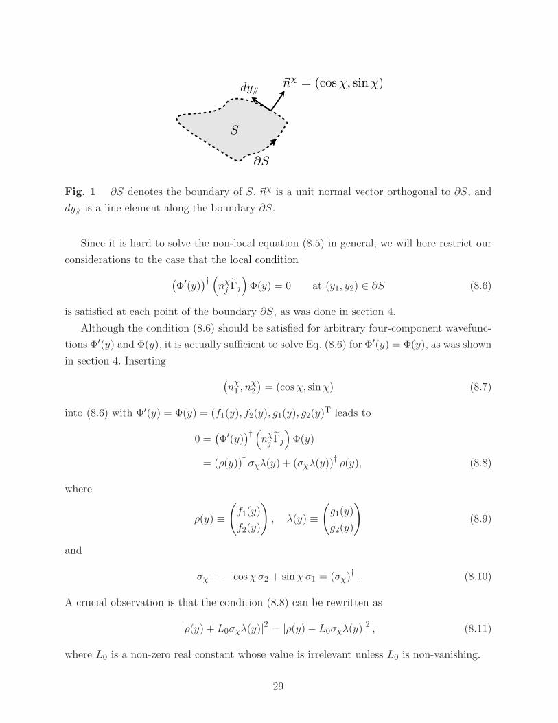
flat surfaces S with boundaries, like polygons, a disk, etc. To this end, we introduce the inner
product for four-component wavefunctions Φ′(y) and Φ(y) on S as
〈Φ′,Φ〉S =
∫
Sdy1dy2
(Φ′(y)
)†Φ(y). (8.1)
The requirement is that the supercharge Q is given by
〈QΦ′,Φ〉S = 〈Φ′, QΦ〉S . (8.2)
By expressing the supercharge Q defined in Eq. (2.14) in the form
Q = i∂yj Γj +M ΓM (j = 1, 2) (8.3)
with
Γ1 =
(0 −σ2−σ2 0
), Γ2 =
(0 σ1
σ1 0
), ΓM =
(0 σ3
σ3 0
), (8.4)
we have found that the condition (8.2) leads to∮
∂Sdy//
(Φ′(y)
)† (nχj Γj
)Φ(y) = 0, (8.5)
where ∂S denotes the boundary of the surface S, (nχ1 , nχ2 ) = (cosχ, sinχ) is a unit normal
vector orthogonal to the boundary ∂S, and dy// is a line element along ∂S, as depicted in
Fig. 1.
28
the form
CP
CP
CP
CP
t, , y) =
[(t, , y (7.17)
where and are CP-transformed fields in the 4d sense. The above transfor-
mation with respect to the extra dimensions is found to correspond to the transformation
(7.2). Thus, we can understand that the 4 matrix originates from the 6d CP transfor-
mation, where ( ) shows the trivial rotation of two-component spinors with an unphysical
overall minus sign.
8 6d Dirac fermion on arbitrary flat surfaces with boundaries
So far, we have restricted our considerations to the rectangle as a two-dimensional extra
space. For phenomenological applications, it will be useful to extend our analysis to arbitrary
flat surfaces with boundaries, like polygons, a disk, etc. To this end, we introduce the inner
product for four-component wavefunctions ) and ) on as
dy dy (8.1)
The requirement that the supercharge is given by
, Q (8.2)
By expressing the supercharge into the form
(8.3)
with
(8.4)
we have found that the condition (8.2) leads to
dy// ) = 0 (8.5)
where denotes the boundary of the surface , ( , n ) = (cos sin ) is a unit normal
vector orthogonal to the boundary , and dy// is a line element along , as depicted in
Fig. ??
28S
∂S
�nχ = (cosχ, sinχ)
Fig. 1 ∂S denotes the boundary of S. ~nχ is a unit normal vector orthogonal to ∂S, and
dy// is a line element along the boundary ∂S.
Since it is hard to solve the non-local equation (8.5) in general, we will here restrict our
considerations to the case that the local condition
(Φ′(y)
)† (nχj Γj
)Φ(y) = 0 at (y1, y2) ∈ ∂S (8.6)
is satisfied at each point of the boundary ∂S, as was done in section 4.
Although the condition (8.6) should be satisfied for arbitrary four-component wavefunc-
tions Φ′(y) and Φ(y), it is actually sufficient to solve Eq. (8.6) for Φ′(y) = Φ(y), as was shown
in section 4. Inserting
(nχ1 , n
χ2
)= (cosχ, sinχ) (8.7)
into (8.6) with Φ′(y) = Φ(y) = (f1(y), f2(y), g1(y), g2(y)T leads to
0 =(Φ′(y)
)† (nχj Γj
)Φ(y)
= (ρ(y))† σχλ(y) + (σχλ(y))† ρ(y), (8.8)
where
ρ(y) ≡(f1(y)
f2(y)
), λ(y) ≡
(g1(y)
g2(y)
)(8.9)
and
σχ ≡ − cosχσ2 + sinχσ1 = (σχ)† . (8.10)
A crucial observation is that the condition (8.8) can be rewritten as
|ρ(y) + L0σχλ(y)|2 = |ρ(y)− L0σχλ(y)|2 , (8.11)
where L0 is a non-zero real constant whose value is irrelevant unless L0 is non-vanishing.
29
General solutions to (8.11) are easily found in the form
ρ(y) + L0σχλ(y) = U (ρ(y)− L0σχλ(y)) , (8.12)
or equivalently
(I2 − U)ρ(y) = −L0(I2 + U)σχλ(y), (8.13)
where U is an arbitrary two-by-two unitary matrix. Following the arguments given in
section 4, we conclude that the condition (8.13) has to reduce to
(I2 − U)ρ(y) = 0, (8.14)
(I2 + U)σχλ(y) = 0, (8.15)
and, further, that the allowed boundary conditions are classified into three types:
1) Type I boundary condition
UType I =
(1 0
0 1
). (8.16)
It follows that the condition (8.14) is trivially satisfied, and the condition (8.15) reduces
to
g1(y) = g2(y) = 0 at (y1, y2) ∈ ∂S. (8.17)
It will be convenient to rewrite the boundary condition (8.17), in terms of the original
four-component wavefunction Φ(y) as
P(−1)F=−1Φ(y) = 0 at (y1, y2) ∈ ∂S, (8.18)
with
P(−1)F=±1 =1
2
(I4 ± (−1)F
). (8.19)
2) Type II boundary condition
30
UType II =
(−1 0
0 −1
). (8.20)
It follows that the condition (8.15) is trivially satisfied, while the condition (8.14) reduces
to
f1(y) = f2(y) = 0 at (y1, y2) ∈ ∂S. (8.21)
In terms of Φ(y), the above boundary condition can be expressed as
P(−1)F=+1Φ(y) = 0 at (y1, y2) ∈ ∂S. (8.22)
3) Type III boundary condition
UType III = ~n · ~σ =
(cos θ e−iφ sin θ
eiφ sin θ − cos θ
), (8.23)
with
~n = (cosφ sin θ, sinφ sin θ, cos θ) . (8.24)
It follows from (8.23) that Eqs. (8.14) and (8.15) become
(I2 − ~n · ~σ)ρ(y) = (I2 − ~n · ~σ)(f1(y)
f2(y)
)= 0,
(I2 + ~n · ~σ′)λ(y) = (I2 + ~n · ~σ′)(g1(y)
g2(y)
)= 0 at (y1, y2) ∈ ∂S, (8.25)
with
~σ′ ≡ σχ~σσχ
= (− cos(2χ)σ1 − sin(2χ)σ2, cos(2χ)σ2 − sin(2χ)σ1,−σ3). (8.26)
Here, we used the property (σχ)2 = I2. It will be convenient to express the above bound-
ary condition in terms of the original four-component wavefunction Φ(y). The result is
given by
P~n·~Σ=−1
Φ(y) = 0 at (y1, y2) ∈ ∂S, (8.27)
where P~n·~Σ=±1
are projection matrices defined by
P~n·~Σ=±1
≡ 1
2
(I4 ± ~n · ~Σ
), (8.28)
~Σ ≡(~σ 0
0 −~σ′
). (8.29)
31
We have succeeded in classifying the allowed boundary conditions at each point of the
boundary ∂S. We should note that the results given in this section are consistent with those
in section 4. Actually, for χ = ±π (χ = ±π/2), the above results reduce to those given in
the subsection 4.2 (4.3).
Let us examine an n-sided polygon as an application of the analysis given above. Let
~nχa = (cosχa, sinχa) (a = 1, 2, . . ., n) be a normal unit vector orthogonal to the ath side of
the polygon. Then, we can impose one of the following boundary conditions on the ath side
of the polygon:
Type I : P(−1)F=−1Φ(y) = 0,
Type II : P(−1)F=+1Φ(y) = 0,
Type III : P~n·~Σa=−1
Φ(y) = 0, (8.30)
with
~Σa =
(~σ 0
0 −σχa~σσχa
). (8.31)
If we would like to impose a single boundary condition on every side of the polygon, the
possible boundary conditions are restricted to
(1) g1(y) = g2(y) = 0,
(2) f1(y) = f2(y) = 0,
(3) f1(y) = g1(y) = 0,
(4) f2(y) = g2(y) = 0, (8.32)
on every side of the polygon. The above boundary conditions (1), (2), (3) and (4) correspond
to Type I, Type II, Type III with θ = π, and Type III with θ = 0, respectively. We note that
the allowed Type III boundary conditions are limited to θ = π and 0, where φ does not
contribute to the boundary conditions at θ = π and 0. This is because the normal unit
vector ~nχa (a = 1, 2, . . ., n) on the ath side is independent of ~nχb for a 6= b, in general, so
that P~n·~Σa=−1
(a = 1, 2, . . ., n) cannot be identical for all sides of the polygon expect for
θ = π and 0, irrespective of φ.
Let us finally discuss a disk as the extra dimensions. For a disk, we may impose a single
boundary condition on every point of the edge of the disk. It then follows from the analysis
of the n-sided polygon that the boundary condition on the edge of the disk has to be chosen
from one of the four boundary conditions (8.32), otherwise the Hermiticity of the supercharge
would be lost.
32
9 Conclusions and discussions
We have succeeded in revealing the supersymmetric structure hidden in the 6d Dirac
action on a rectangle. The supersymmetry turns out to be very useful to classify the class
of allowed boundary conditions, and to clarify the 4d mass spectrum of the Kaluza–Klein
modes for the 6d Dirac fermion. In fact, the allowed boundary conditions are derived by
demanding the Hermiticity of the supercharge and are classified into three types. We have
furthermore extended our analysis to arbitrary flat surfaces as the two-dimensional extra
space. We have then found that the supersymmetric structure is still realized there and have
succeeded in classifying the allowed boundary conditions, in general.
An important observation in our results is that two massless chiral fermions appear in
the 4d mass spectrum for the Type I or Type II boundary conditions. This result seems to be
surprising because the 6d Dirac fermion is non-chiral and furthermore has the non-vanishing
bulk mass M .14 Then, one might naively expect that the 4d mass spectrum would consist
of only massive states with masses heavier than M . Actually, positive-energy eigenstates
correspond to massive 4d Dirac fermions with masses mn1n2 > M for n1, n2 = 1, 2, 3, . . ..
On the other hand, we have found that the 4d massless chiral fermions correspond to zero-
energy solutions, which are bound states and possess a topological nature in supersymmetric
quantum mechanics. The appearance of the degenerate 4d massless chiral fermions will
become crucially important in solving the generation problem and also the fermion mass
hierarchy problem of the quarks and leptons, though the 4d massless chiral fermions are
two-fold degenerate but not three- in the present 6d model.
In our analysis, we have found the remarkable feature that zero-energy solutions are
not affected by the presence of the boundaries, while the boundary conditions work well
for determining the positive-energy solutions. Even though we have explicitly constructed a
one-parameter family of the zero-energy solutions (5.18) and (5.22) for the Type II boundary
condition and shown that the number of the degeneracy is two, the analysis seems to be
insufficient. This is because the general class of the zero-energy solutions is much wider than
considered here, and we have not succeeded in determining a complete set of zero-energy
solutions definitely.15 Since zero-energy solutions are directly related to massless 4d chiral
fermions, it would be of great importance to clarify the structure of the zero-energy solutions
14 It should be emphasized that no zero-energy solution or no 4d massless chiral fermion appears for the
non-vanishing bulk mass M if we take the torus as the two-dimensional extra space, instead of the rectangle.15 It is worth noting that no trouble appears in 5d fermion systems with a single extra dimension, though
a similar situation happens there [30–32, 34]. Any zero-energy solution is not degenerate in one dimension,
so that it can be determined uniquely.
33
for higher-dimensional Dirac systems with more than or equal to two extra dimensions,
phenomenologically as well as mathematically.16
One extension of our analysis is to introduce potential terms in the Hamiltonian. This
can be done by replacing the bulk mass M by a superpotential W (y) in the supercharge Q
in (2.14). Even with the superpotential W (y), the supercharge is still Hermitian for Type I,
II and III boundary conditions. Interestingly, the superpotential may naturally be introduced
through a Yukawa interaction g〈φ(y)〉Ψ(x, y)Ψ(x, y) with a non-trivial background 〈φ(y)〉 ofa scalar field φ(x, y).
Another important extension of our analysis is to investigate higher-dimensional Dirac
actions. In the case of a 6d Dirac fermion, only two massless chiral fermions appear in the
4d mass spectrum, which is not sufficient to solve the generation problem. However, more
than two 4d massless chiral fermions may appear in the case of higher dimensions, equal to
or more than eight dimensions, even though it is naively expected that 2n massless chiral
fermions would appear in the case ofD = 4 + 2n. This may imply that it is very important to
perform a comprehensive analysis of the allowed boundary conditions in higher-dimensional
Dirac actions, as done in this paper, because a suitable choice of boundary conditions could
reduce the possible 2n massless chiral fermions to three massless ones. Thus, it would be of
great interest to extend our analysis to higher-dimensional Dirac fermions and to search for
the possibility of producing a three-generation model. This work will be reported elsewhere.
Acknowledgments
We thank Tomoaki Nagasawa for discussions in the early stages of this work. This work is
supported in part by Grants-in-Aid for Scientific Research [No. 15K05055 and No. 25400260
(M.S.)] from the Ministry of Education, Culture, Sports, Science and Technology (MEXT)
in Japan.
16 Determining the size and the shape of the extra dimensions, known as moduli stabilization, would
be issues closely related to gravitational effects in higher-dimensional space-time, which is absent in the
present flat setup. Though this subject is of importance for a complete discussion on models in the context
of extra dimension, we will leave it for a topics for future studies. Another extension is to consider curved
extra dimensions. Even for this situation, the supersymmetric structure is expected to be realized [39, 42].
It would be of interest to study the above subjects.
34
Appendix
A Chiral representation of 6d Gamma matrices
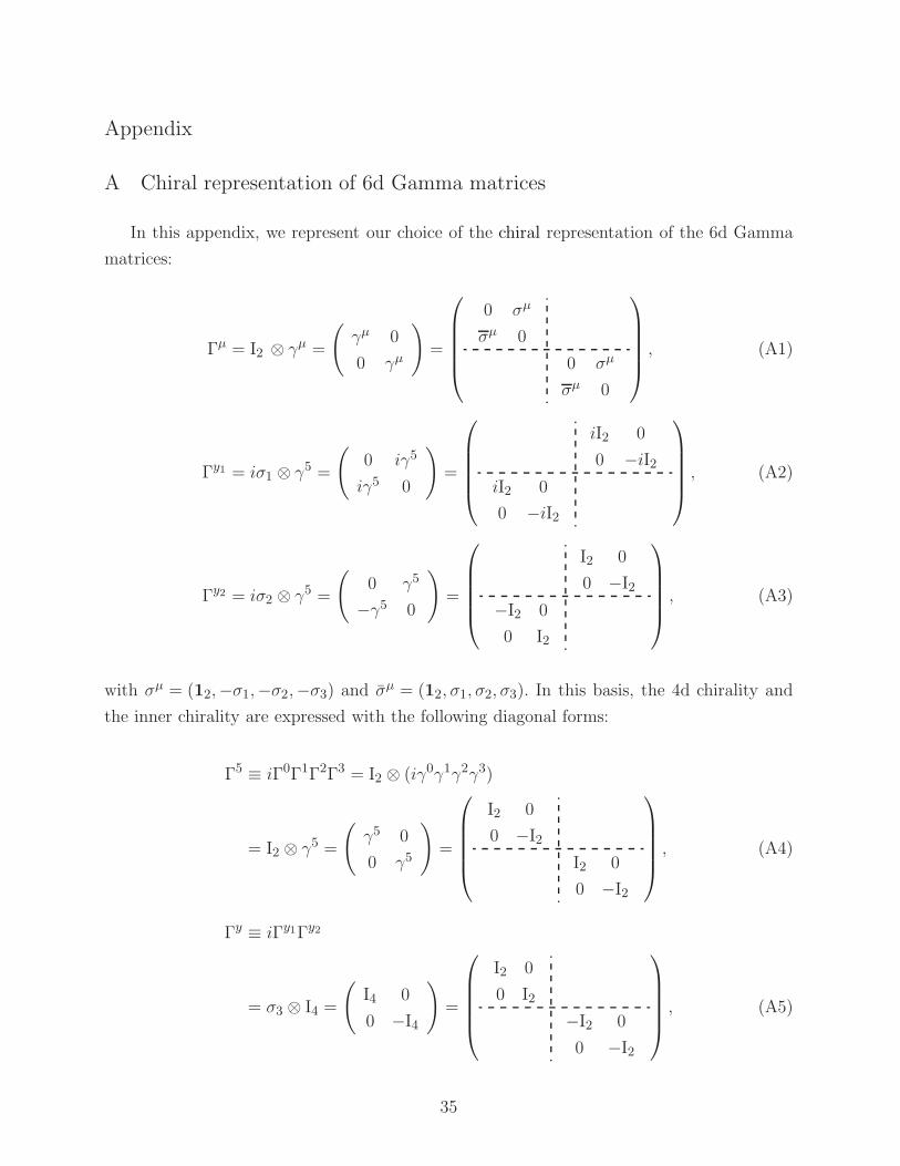
In this appendix, we represent our choice of the chiral representation of the 6d Gamma
matrices:
Γµ = I2 ⊗ γµ =
(γµ 0
0 γµ
)=
0 σµ
σµ 0
0 σµ
σµ 0
, (A1)
Γy1 = iσ1 ⊗ γ5 =(
0 iγ5
iγ5 0
)=
iI2 0
0 −iI2iI2 0
0 −iI2
, (A2)
Γy2 = iσ2 ⊗ γ5 =(
0 γ5
−γ5 0
)=
I2 0
0 −I2−I2 0
0 I2
, (A3)
with σµ = (12,−σ1,−σ2,−σ3) and σµ = (12, σ1, σ2, σ3). In this basis, the 4d chirality and
the inner chirality are expressed with the following diagonal forms:
Γ5 ≡ iΓ0Γ1Γ2Γ3 = I2 ⊗ (iγ0γ1γ2γ3)
= I2 ⊗ γ5 =(γ5 0
0 γ5
)=
I2 0
0 −I2I2 0
0 −I2
, (A4)
Γy ≡ iΓy1Γy2
= σ3 ⊗ I4 =
(I4 0
0 −I4
)=
I2 0
0 I2
−I2 0
0 −I2
, (A5)
35
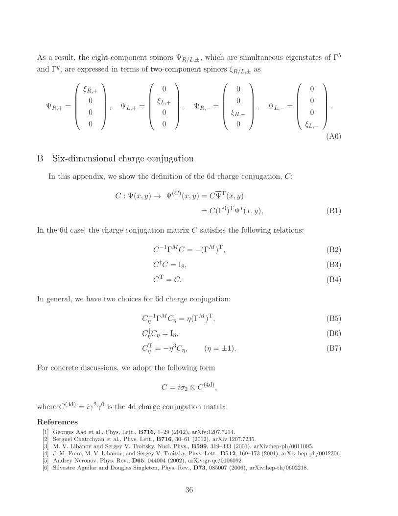
As a result, the eight-component spinors ΨR/L,±, which are simultaneous eigenstates of Γ5
and Γy, are expressed in terms of two-component spinors ξR/L,± as
ΨR,+ =
ξR,+
0
0
0
, ΨL,+ =
0
ξL,+
0
0
, ΨR,− =
0
0
ξR,−
0
, ΨL,− =
0
0
0
ξL,−
.
(A6)
B Six-dimensional charge conjugation
In this appendix, we show the definition of the 6d charge conjugation, C:
C : Ψ(x, y)→ Ψ(C)(x, y) = CΨT(x, y)
= C(Γ0)TΨ∗(x, y), (B1)
In the 6d case, the charge conjugation matrix C satisfies the following relations:
C−1ΓMC = −(ΓM )T, (B2)
C†C = I8, (B3)
CT = C. (B4)
In general, we have two choices for 6d charge conjugation:
C−1η ΓMCη = η(ΓM )T, (B5)
C†ηCη = I8, (B6)
CTη = −η3Cη, (η = ±1). (B7)
For concrete discussions, we adopt the following form
C = iσ2 ⊗ C(4d),
where C(4d) = iγ2γ0 is the 4d charge conjugation matrix.
References
[1] Georges Aad et al., Phys. Lett., B716, 1–29 (2012), arXiv:1207.7214.[2] Serguei Chatrchyan et al., Phys. Lett., B716, 30–61 (2012), arXiv:1207.7235.[3] M. V. Libanov and Sergey V. Troitsky, Nucl. Phys., B599, 319–333 (2001), arXiv:hep-ph/0011095.[4] J. M. Frere, M. V. Libanov, and Sergey V. Troitsky, Phys. Lett., B512, 169–173 (2001), arXiv:hep-ph/0012306.[5] Andrey Neronov, Phys. Rev., D65, 044004 (2002), arXiv:gr-qc/0106092.[6] Silvestre Aguilar and Douglas Singleton, Phys. Rev., D73, 085007 (2006), arXiv:hep-th/0602218.
36
[7] Merab Gogberashvili, Pavle Midodashvili, and Douglas Singleton, JHEP, 08, 033 (2007), arXiv:0706.0676.[8] Zhi-qiang Guo and Bo-Qiang Ma, JHEP, 08, 065 (2008), arXiv:0808.2136.[9] David B. Kaplan and Sichun Sun, Phys. Rev. Lett., 108, 181807 (2012), arXiv:1112.0302.
[10] Nima Arkani-Hamed and Martin Schmaltz, Phys. Rev., D61, 033005 (2000), arXiv:hep-ph/9903417.[11] G. R. Dvali and Mikhail A. Shifman, Phys. Lett., B475, 295–302 (2000), arXiv:hep-ph/0001072.[12] Tony Gherghetta and Alex Pomarol, Nucl. Phys., B586, 141–162 (2000), arXiv:hep-ph/0003129.[13] David Elazzar Kaplan and Timothy M.P. Tait, Journal of High Energy Physics, 2000(06), 020 (2000).[14] David Elazzar Kaplan and Timothy M. P. Tait, JHEP, 11, 051 (2001), arXiv:hep-ph/0110126.[15] Stephan J. Huber and Qaisar Shafi, Phys. Lett., B498, 256–262 (2001), arXiv:hep-ph/0010195.[16] Mitsuru Kakizaki and Masahiro Yamaguchi, Int. J. Mod. Phys., A19, 1715–1736 (2004), arXiv:hep-ph/0110266.[17] Naoyuki Haba, Atsushi Watanabe, and Koichi Yoshioka, Phys. Rev. Lett., 97, 041601 (2006), arXiv:hep-
ph/0603116.[18] Hiroyuki Abe, Kang-Sin Choi, Tatsuo Kobayashi, and Hiroshi Ohki, Nucl. Phys., B814, 265–292 (2009),
arXiv:0812.3534.[19] Csaba Csaki, Cedric Delaunay, Christophe Grojean, and Yuval Grossman, JHEP, 10, 055 (2008),
arXiv:0806.0356.[20] Hiroyuki Abe, Tatsuo Kobayashi, Hiroshi Ohki, Akane Oikawa, and Keigo Sumita, Nucl. Phys., B870, 30–54
(2013), arXiv:1211.4317.[21] S. Randjbar-Daemi, Abdus Salam, and J. A. Strathdee, Nucl. Phys., B214, 491–512 (1983).[22] D. Cremades, L. E. Ibanez, and F. Marchesano, JHEP, 05, 079 (2004), arXiv:hep-th/0404229.[23] Hiroyuki Abe, Tatsuo Kobayashi, and Hiroshi Ohki, JHEP, 09, 043 (2008), arXiv:0806.4748.[24] Yukihiro Fujimoto, Tatsuo Kobayashi, Takashi Miura, Kenji Nishiwaki, and Makoto Sakamoto, Phys. Rev.,
D87(8), 086001 (2013), arXiv:1302.5768.[25] Tomo-Hiro Abe, Yukihiro Fujimoto, Tatsuo Kobayashi, Takashi Miura, Kenji Nishiwaki, and Makoto Sakamoto,
JHEP, 01, 065 (2014), arXiv:1309.4925.[26] Tomo-hiro Abe, Yukihiro Fujimoto, Tatsuo Kobayashi, Takashi Miura, Kenji Nishiwaki, and Makoto Sakamoto,
Nucl. Phys., B890, 442–480 (2014), arXiv:1409.5421.[27] Tomo-hiro Abe, Yukihiro Fujimoto, Tatsuo Kobayashi, Takashi Miura, Kenji Nishiwaki, Makoto Sakamoto,
and Yoshiyuki Tatsuta, Nucl. Phys., B894, 374–406 (2015), arXiv:1501.02787.[28] Yoshio Matsumoto and Yutaka Sakamura, PTEP, 2016(5), 053B06 (2016), arXiv:1602.01994.[29] Yukihiro Fujimoto, Tatsuo Kobayashi, Kenji Nishiwaki, Makoto Sakamoto, and Yoshiyuki Tatsuta, Phys. Rev.,
D94, 035031 (2016), arXiv:1605.00140.[30] Yukihiro Fujimoto, Tomoaki Nagasawa, Kenji Nishiwaki, and Makoto Sakamoto, PTEP, 2013, 023B07 (2013),
arXiv:1209.5150.[31] Yukihiro Fujimoto, Kenji Nishiwaki, and Makoto Sakamoto, Phys. Rev., D88(11), 115007 (2013),
arXiv:1301.7253.[32] Yukihiro Fujimoto, Kenji Nishiwaki, Makoto Sakamoto, and Ryo Takahashi, JHEP, 10, 191 (2014),
arXiv:1405.5872.[33] Chengfeng Cai and Hong-Hao Zhang, Phys. Rev., D93(3), 036003 (2016), arXiv:1503.08805.[34] Yukihiro Fujimoto, Tomoaki Nagasawa, Satoshi Ohya, and Makoto Sakamoto, Prog. Theor. Phys., 126, 841–854
(2011), arXiv:1108.1976.[35] Yukihiro Fujimoto, Kouhei Hasegawa, Kenji Nishiwaki, Makoto Sakamoto, and Kentaro Tatsumi (2016),
arXiv:1609.01413.[36] O. DeWolfe, D. Z. Freedman, S. S. Gubser, and A. Karch, Phys. Rev., D62, 046008 (2000), arXiv:hep-
th/9909134.[37] Andre Miemiec, Fortsch. Phys., 49, 747–755 (2001), arXiv:hep-th/0011160.[38] C. S. Lim, Tomoaki Nagasawa, Makoto Sakamoto, and Hidenori Sonoda, Phys. Rev., D72, 064006 (2005),
arXiv:hep-th/0502022.[39] C. S. Lim, Tomoaki Nagasawa, Satoshi Ohya, Kazuki Sakamoto, and Makoto Sakamoto, Phys. Rev., D77,
045020 (2008), arXiv:0710.0170.[40] C. S. Lim, Tomoaki Nagasawa, Satoshi Ohya, Kazuki Sakamoto, and Makoto Sakamoto, Phys. Rev., D77,
065009 (2008), arXiv:0801.0845.[41] Satoshi Ohya, SUSY QM meets 5d Gravity, In Supersymmetric quantum mechanics and spectral design.
Proceedings, Workshop, Benasque, Spain, July 18-30, 2010 (2010), arXiv:1012.0301.[42] Tomoaki Nagasawa, Satoshi Ohya, Kazuki Sakamoto, and Makoto Sakamoto, SIGMA, 7, 065 (2011),
arXiv:1105.4829.[43] Makoto Sakamoto (2012), arXiv:1201.2448.[44] M. Williams, C. P. Burgess, L. van Nierop, and A. Salvio, JHEP, 01, 102 (2013), arXiv:1210.3753.
37
[45] C. P. Burgess, L. van Nierop, S. Parameswaran, A. Salvio, and M. Williams, JHEP, 02, 120 (2013),arXiv:1210.5405.
[46] Edward Witten, Nucl. Phys., B188, 513 (1981).[47] Fred Cooper, Avinash Khare, and Uday Sukhatme, Phys. Rept., 251, 267–385 (1995), arXiv:hep-th/9405029.[48] F. Cooper, A. Khare, and U. Sukhatme, Supersymmetry in quantum mechanics, 2001).[49] Taksu Cheon, Tamas Fulop, and Izumi Tsutsui, Annals Phys., 294, 1–23 (2001), arXiv:quant-ph/0008123.[50] Tomoaki Nagasawa, Satoshi Ohya, Kazuki Sakamoto, Makoto Sakamoto, and Kosuke Sekiya, J. Phys., A42,
265203 (2009), arXiv:0812.4659.[51] C. S. Lim, Phys. Lett., B256, 233–238 (1991).[52] C. S. Lim, Nobuhito Maru, and Kenji Nishiwaki, Phys. Rev., D81, 076006 (2010), arXiv:0910.2314.[53] Tatsuo Kobayashi, Kenji Nishiwaki, and Yoshiyuki Tatsuta, JHEP, 04, 080 (2017), arXiv:1609.08608.
38