Embed Size (px)
Citation preview
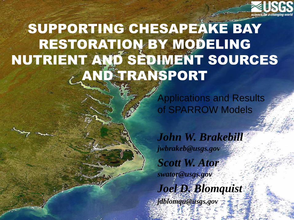
SUPPORTING CHESAPEAKE BAY
RESTORATION BY MODELING
NUTRIENT AND SEDIMENT SOURCES
AND TRANSPORT
Applications and Results
of SPARROW Models
John W. [email protected]
Scott W. [email protected]
Joel D. [email protected]
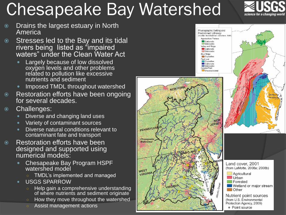
Chesapeake Bay Watershed Drains the largest estuary in North
America
Stresses led to the Bay and its tidal rivers being listed as “impaired waters” under the Clean Water Act Largely because of low dissolved
oxygen levels and other problems related to pollution like excessive nutrients and sediment
Imposed TMDL throughout watershed
Restoration efforts have been ongoing for several decades.
Challenges: Diverse and changing land uses
Variety of contaminant sources
Diverse natural conditions relevant to contaminant fate and transport
Restoration efforts have been designed and supported using numerical models: Chesapeake Bay Program HSPF
watershed model○ TMDL’s implemented and managed
USGS SPARROW○ Help gain a comprehensive understanding
of where nutrients and sediment originate
○ How they move throughout the watershed
○ Assist management actions
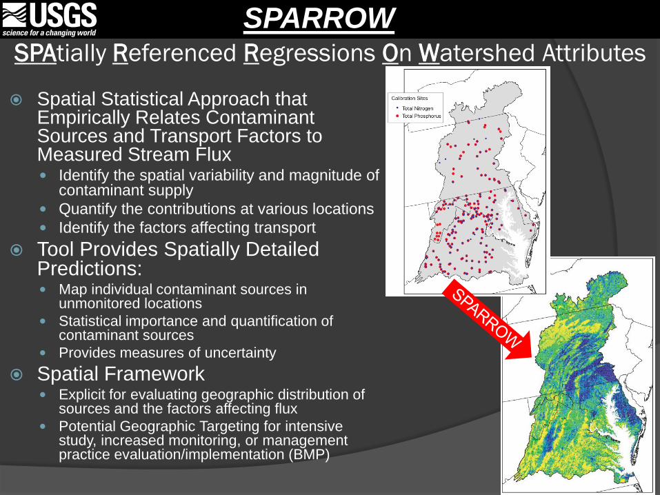
SPAtially Referenced Regressions On Watershed Attributes
Spatial Statistical Approach that Empirically Relates Contaminant Sources and Transport Factors to Measured Stream Flux Identify the spatial variability and magnitude of
contaminant supply
Quantify the contributions at various locations
Identify the factors affecting transport
Tool Provides Spatially Detailed Predictions: Map individual contaminant sources in
unmonitored locations
Statistical importance and quantification of contaminant sources
Provides measures of uncertainty
Spatial Framework Explicit for evaluating geographic distribution of
sources and the factors affecting flux
Potential Geographic Targeting for intensive study, increased monitoring, or management practice evaluation/implementation (BMP)
SPARROW
Water Quality
Streamflow
Mean annual flux
Standardized
Sediment Sources
– Atmospheric
– Urban
– Agricultural
– Forest
– Point
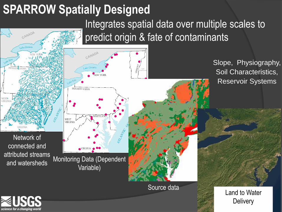
NHDPlus 1:100,000
Flow and Velocity
Watersheds for
each reach
Network of
connected and
attributed streams
and watershedsMonitoring Data (Dependent
Variable)
Source data
Slope, Physiography,
Soil Characteristics,
Reservoir Systems
SPARROW Spatially DesignedIntegrates spatial data over multiple scales to
predict origin & fate of contaminants
Land to Water
Delivery
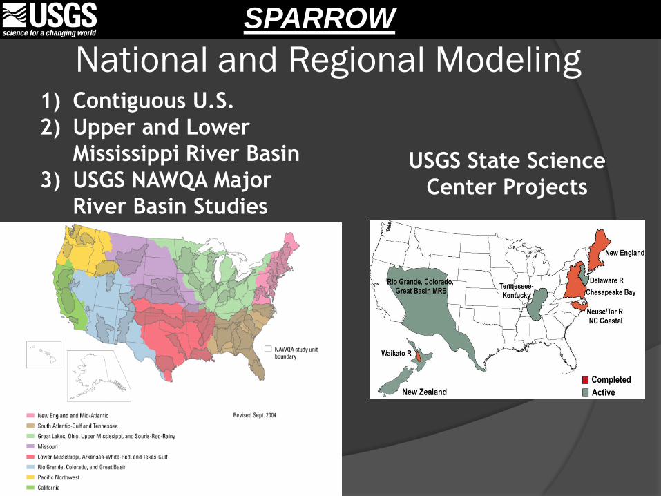
USGS State Science
Center Projects
1) Contiguous U.S.
2) Upper and Lower
Mississippi River Basin
3) USGS NAWQA Major
River Basin Studies
SPARROW
National and Regional Modeling
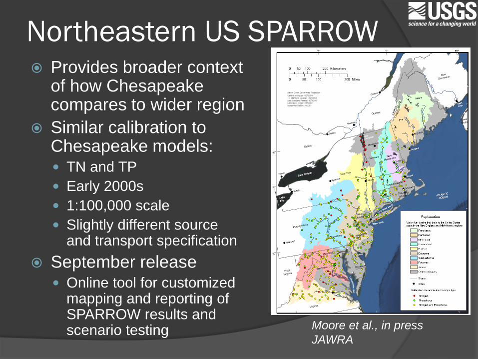
Northeastern US SPARROW Provides broader context
of how Chesapeake compares to wider region
Similar calibration to Chesapeake models: TN and TP
Early 2000s
1:100,000 scale
Slightly different source and transport specification
September release Online tool for customized
mapping and reporting of SPARROW results and scenario testing Moore et al., in press
JAWRA
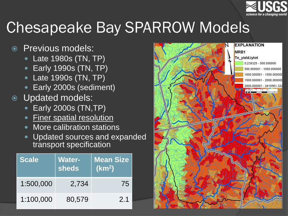
Chesapeake Bay SPARROW Models
Previous models: Late 1980s (TN, TP)
Early 1990s (TN, TP)
Late 1990s (TN, TP)
Early 2000s (sediment)
Updated models: Early 2000s (TN,TP)
Finer spatial resolution
More calibration stations
Updated sources and expanded transport specification
Scale Water-
sheds
Mean Size
(km2)
1:500,000 2,734 75
1:100,000 80,579 2.1
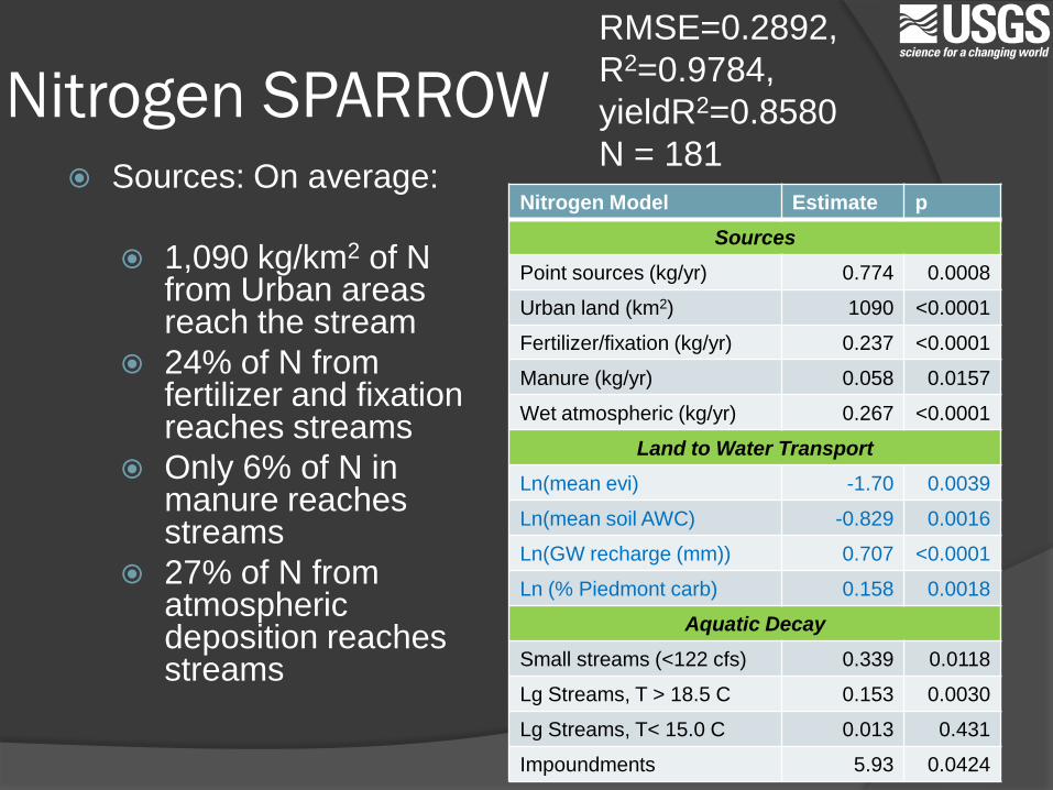
Nitrogen SPARROW
Nitrogen Model Estimate p
Sources
Point sources (kg/yr) 0.774 0.0008
Urban land (km2) 1090 <0.0001
Fertilizer/fixation (kg/yr) 0.237 <0.0001
Manure (kg/yr) 0.058 0.0157
Wet atmospheric (kg/yr) 0.267 <0.0001
Land to Water Transport
Ln(mean evi) -1.70 0.0039
Ln(mean soil AWC) -0.829 0.0016
Ln(GW recharge (mm)) 0.707 <0.0001
Ln (% Piedmont carb) 0.158 0.0018
Aquatic Decay
Small streams (<122 cfs) 0.339 0.0118
Lg Streams, T > 18.5 C 0.153 0.0030
Lg Streams, T< 15.0 C 0.013 0.431
Impoundments 5.93 0.0424
Sources: On average:
1,090 kg/km2 of N from Urban areas reach the stream
24% of N from fertilizer and fixation reaches streams
Only 6% of N in manure reaches streams
27% of N from atmospheric deposition reaches streams
RMSE=0.2892,
R2=0.9784,
yieldR2=0.8580
N = 181
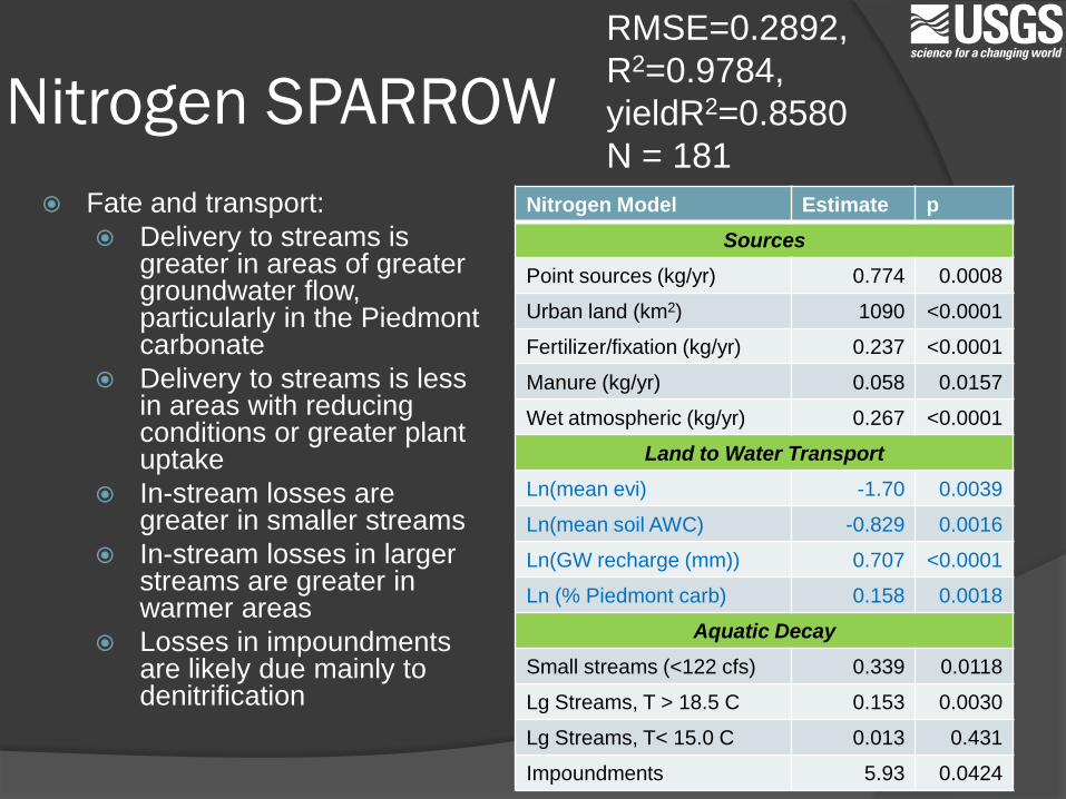
Nitrogen SPARROW
Fate and transport:
Delivery to streams is greater in areas of greater groundwater flow, particularly in the Piedmont carbonate
Delivery to streams is less in areas with reducing conditions or greater plant uptake
In-stream losses are greater in smaller streams
In-stream losses in larger streams are greater in warmer areas
Losses in impoundmentsare likely due mainly to denitrification
Nitrogen Model Estimate p
Sources
Point sources (kg/yr) 0.774 0.0008
Urban land (km2) 1090 <0.0001
Fertilizer/fixation (kg/yr) 0.237 <0.0001
Manure (kg/yr) 0.058 0.0157
Wet atmospheric (kg/yr) 0.267 <0.0001
Land to Water Transport
Ln(mean evi) -1.70 0.0039
Ln(mean soil AWC) -0.829 0.0016
Ln(GW recharge (mm)) 0.707 <0.0001
Ln (% Piedmont carb) 0.158 0.0018
Aquatic Decay
Small streams (<122 cfs) 0.339 0.0118
Lg Streams, T > 18.5 C 0.153 0.0030
Lg Streams, T< 15.0 C 0.013 0.431
Impoundments 5.93 0.0424
RMSE=0.2892,
R2=0.9784,
yieldR2=0.8580
N = 181
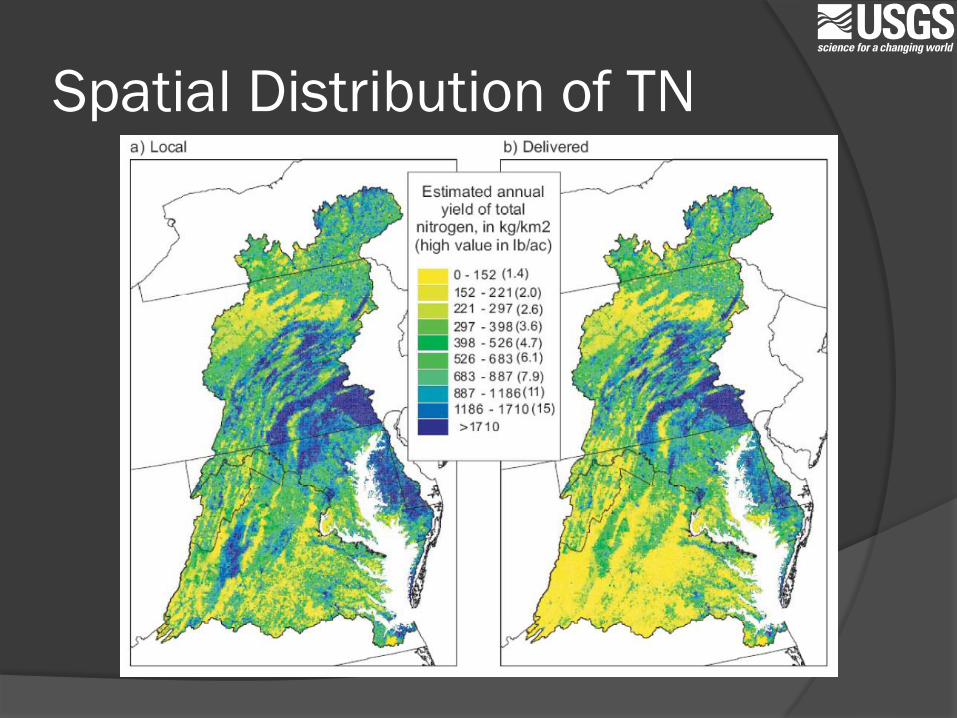
Spatial Distribution of TN
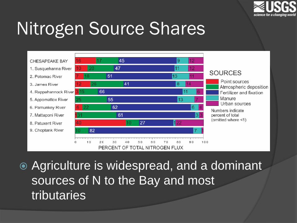
Nitrogen Source Shares
Agriculture is widespread, and a dominant
sources of N to the Bay and most
tributaries
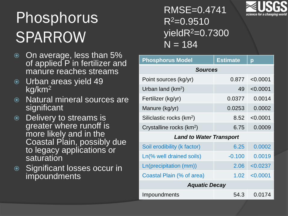
Phosphorus
SPARROW
Phosphorus Model Estimate p
Sources
Point sources (kg/yr) 0.877 <0.0001
Urban land (km2) 49 <0.0001
Fertilizer (kg/yr) 0.0377 0.0014
Manure (kg/yr) 0.0253 0.0002
Siliclastic rocks (km2) 8.52 <0.0001
Crystalline rocks (km2) 6.75 0.0009
Land to Water Transport
Soil erodibility (k factor) 6.25 0.0002
Ln(% well drained soils) -0.100 0.0019
Ln(precipitation (mm)) 2.06 <0.0237
Coastal Plain (% of area) 1.02 <0.0001
Aquatic Decay
Impoundments 54.3 0.0174
On average, less than 5% of applied P in fertilizer and manure reaches streams
Urban areas yield 49 kg/km2
Natural mineral sources are significant
Delivery to streams is greater where runoff is more likely and in the Coastal Plain, possibly due to legacy applications or saturation
Significant losses occur in impoundments
RMSE=0.4741
R2=0.9510
yieldR2=0.7300
N = 184
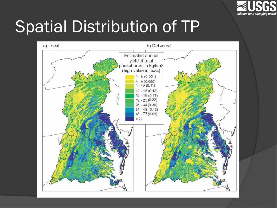
Spatial Distribution of TP
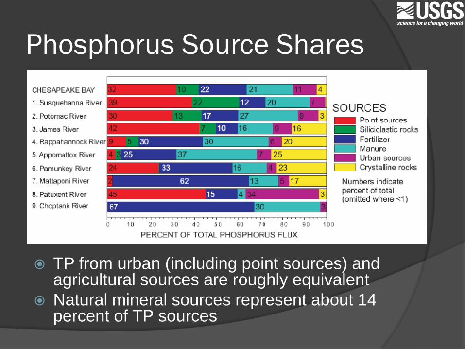
Phosphorus Source Shares
TP from urban (including point sources) and agricultural sources are roughly equivalent
Natural mineral sources represent about 14 percent of TP sources
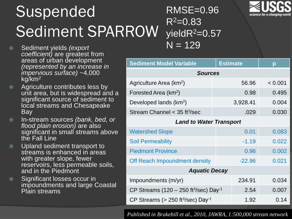
Suspended
Sediment SPARROW
Sediment Model Variable Estimate p
Sources
Agriculture Area (km2) 56.96 < 0.001
Forested Area (km2) 0.98 0.495
Developed lands (km2) 3,928.41 0.004
Stream Channel < 35 ft3/sec .029 0.030
Land to Water Transport
Watershed Slope 0.01 0.083
Soil Permeability -1.19 0.022
Piedmont Province 0.96 0.002
Off Reach Impoundment density -22.96 0.021
Aquatic Decay
Impoundments (m/yr) 234.91 0.034
CP Streams (120 – 250 ft3/sec) Day-1 2.54 0.007
CP Streams (> 250 ft3/sec) Day-1 1.92 0.14
Sediment yields (export coefficient) are greatest from areas of urban development (represented by an increase in impervious surface) ~4,000 kg/km2
Agriculture contributes less by unit area, but is widespread and a significant source of sediment to local streams and Chesapeake Bay
In-stream sources (bank, bed, or flood plain erosion) are also significant in small streams above the Fall Line
Upland sediment transport to streams is enhanced in areas with greater slope, fewer reservoirs, less permeable soils, and in the Piedmont
Significant losses occur in impoundments and large Coastal Plain streams
RMSE=0.96
R2=0.83
yieldR2=0.57
N = 129
Published in Brakebill et al., 2010, JAWRA, 1:500,000 stream network
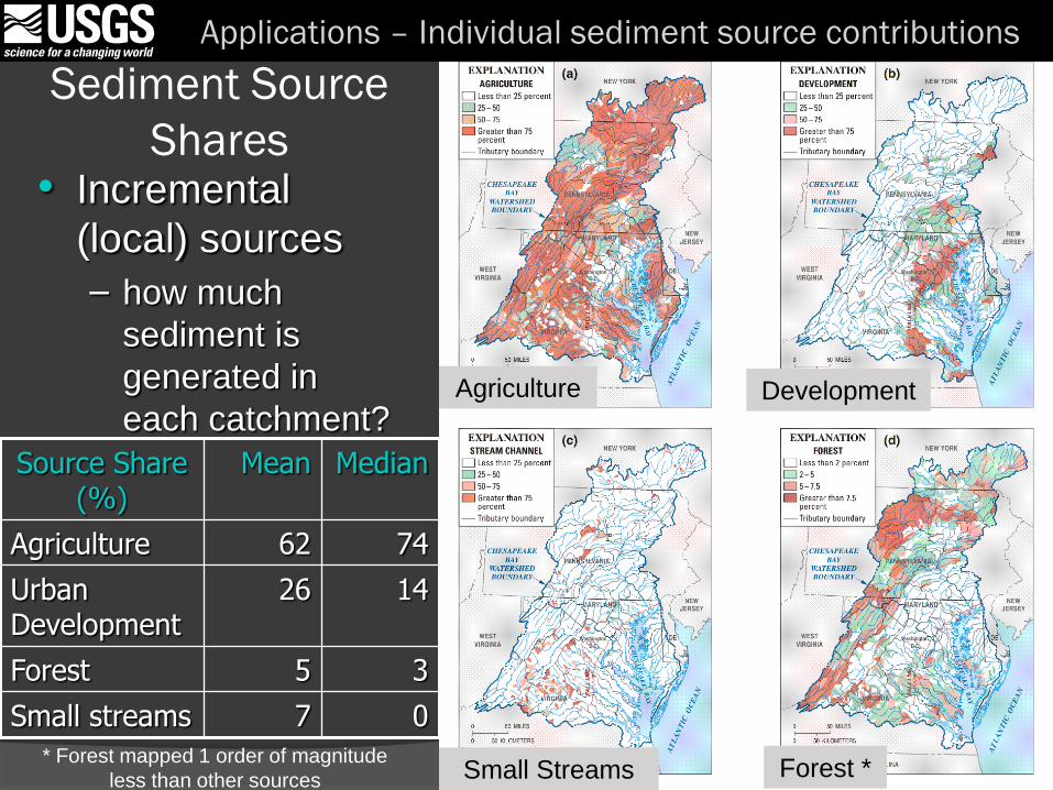
Applications – Individual sediment source contributions
Sediment Source
Shares
Agriculture Development
Small Streams Forest *
• Incremental
(local) sources
– how much
sediment is
generated in
each catchment?
Source Share (%)
Mean Median
Agriculture 62 74
Urban Development
26 14
Forest 5 3
Small streams 7 0
* Forest mapped 1 order of magnitude
less than other sources
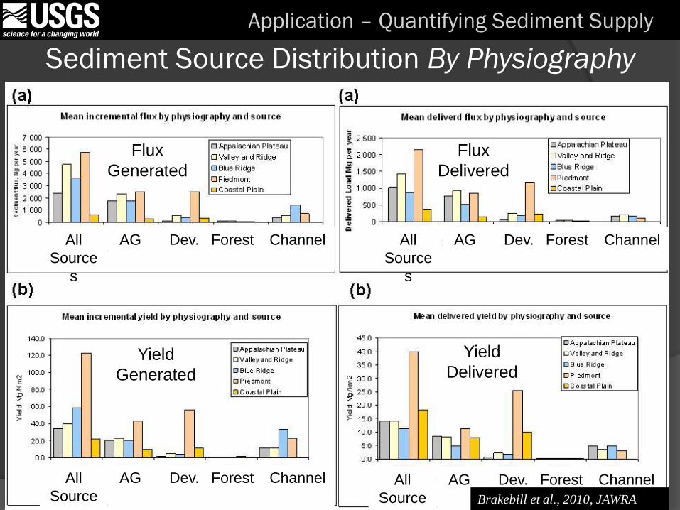
Sediment Source Distribution By Physiography
Application – Quantifying Sediment Supply
Flux
Delivered
Yield
Generated
Yield
Delivered
Flux
Generated
AG Dev. ChannelAll
Source
s
Forest
AG Dev. ChannelAll
Source
s
Forest
AG Dev. ChannelAll
Source
s
Forest
AG Dev. ChannelAll
Source
s
Forest
Brakebill et al., 2010, JAWRA
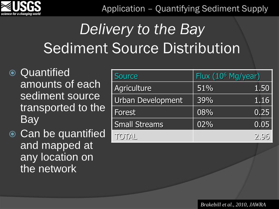
Delivery to the Bay
Sediment Source Distribution
Quantified amounts of each sediment source transported to the Bay
Can be quantified and mapped at any location on the network
Source Flux (106 Mg/year)
Agriculture 51% 1.50
Urban Development 39% 1.16
Forest 08% 0.25
Small Streams 02% 0.05
TOTAL 2.96
Application – Quantifying Sediment Supply
Brakebill et al., 2010, JAWRA
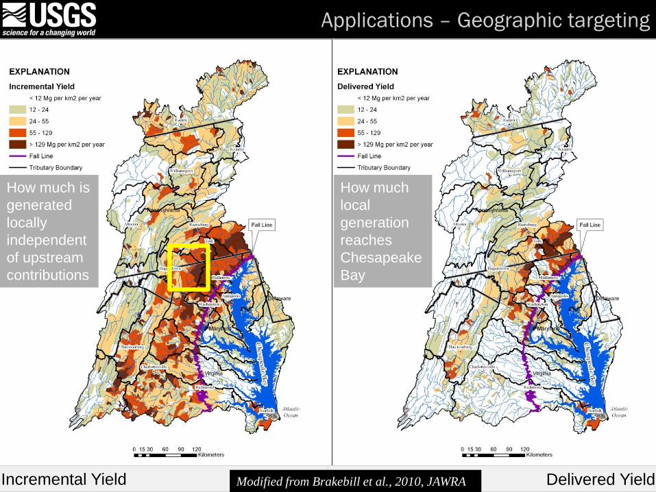
Applications – Geographic targeting
Incremental Yield Delivered Yield
How much
local
generation
reaches
Chesapeake
Bay
How much is
generated
locally
independent
of upstream
contributions
Modified from Brakebill et al., 2010, JAWRA
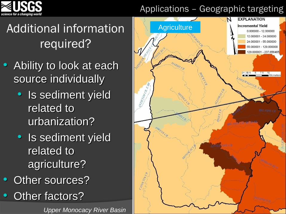
Additional information
required?
Applications – Geographic targeting
• Ability to look at each
source individually
• Is sediment yield
related to
urbanization?
• Is sediment yield
related to
agriculture?
• Other sources?
• Other factors?Upper Monocacy River Basin
All SourcesUrbanizationAgriculture
Applying the SPARROW model provides the ability to gain a regional understanding of contaminant supply, fate, and transport within the Chesapeake Bay watershed The SPARROW model demonstrates reasonable relations between the
response variable (long-term water-quality conditions) and selected exploratory data representing supply, transport, and storage (Model diagnostics).
Model evaluations and predictions are directly applicable to nutrient and sediment management in watersheds of estuaries like Chesapeake Bay: Identifying individual source contributions and their relative importance
Identifying important transport factors and their relative importance
Quantifying relative amounts of sediment generated and transported to Chesapeake Bay
Enhanced geographic targeting tool for further study, additional monitoring, or prioritizing management actions for a variety of sources and settings
Seeking out and working with State and Local agencies to better provide information suited for their needs
Applications
2002 North East Nitrogen and Phosphorus SPARROW models
September. 2011
1:100,000 scale
JAWRA
Online tool (DSS) for customized mapping and reporting of SPARROW results and scenario testing
2002 Chesapeake Bay Nitrogen and Phosphorus SPARROW models
Last quarter, 2011
1:100,000 scale
USGS SIR Report ( including predictions)
Also available in DSS (soon after publication) for customized mapping and reporting of SPARROW results and scenario testing
2002 Chesapeake Bay Suspended Sediment model – Published
1:500,000 scale
JAWRA
http://onlinelibrary.wiley.com/doi/10.1111/j.1752-1688.2010.00450.x/abstract
Information
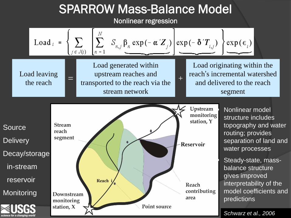
SPARROW Mass-Balance ModelNonlinear regression
Load leaving
the reach=
Load generated within
upstream reaches and
transported to the reach via the
stream network
+
Load originating within the
reach’s incremental watershed
and delivered to the reach
segment
Nonlinear model
structure includes
topography and water
routing; provides
separation of land and
water processes
Steady-state, mass-
balance structure
gives improved
interpretability of the
model coefficients and
predictions
Source
Delivery
Decay/storage
in-stream
reservoir
Monitoring
Schwarz et al., 2006
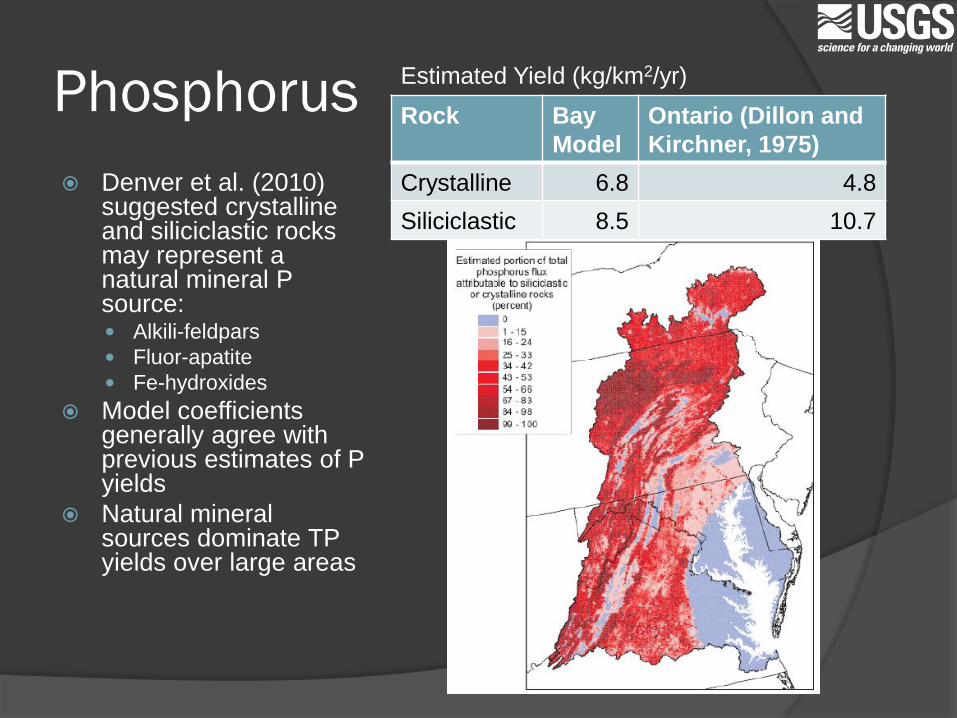
Phosphorus
Denver et al. (2010) suggested crystalline and siliciclastic rocks may represent a natural mineral P source: Alkili-feldpars
Fluor-apatite
Fe-hydroxides
Model coefficients generally agree with previous estimates of P yields
Natural mineral sources dominate TP yields over large areas
Rock Bay
Model
Ontario (Dillon and
Kirchner, 1975)
Crystalline 6.8 4.8
Siliciclastic 8.5 10.7
Estimated Yield (kg/km2/yr)
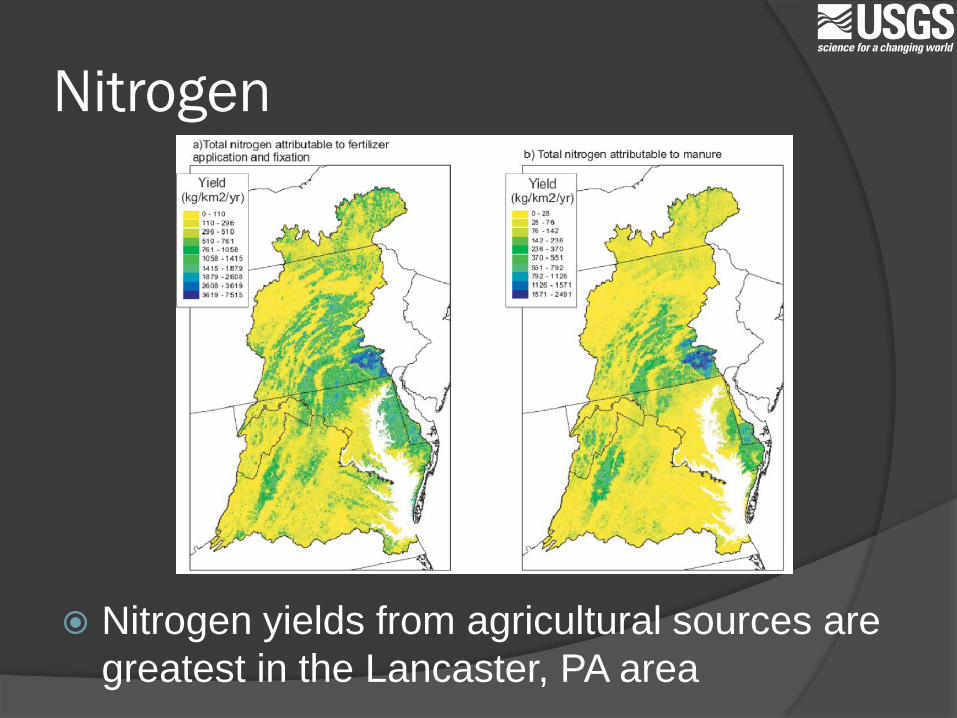
Nitrogen
Nitrogen yields from agricultural sources are
greatest in the Lancaster, PA area