Embed Size (px)
Citation preview

www.pnas.org/cgi/doi/10.1073/pnas. 115
Supporting Materials forThe differential coding of perception in the
world’s languages
Asifa Majid, Sean G. Roberts, Ludy Cilissen,Karen Emmorey, Brenda Nicodemus, Lucinda O’Grady,
Bencie Woll, Barbara LeLan, Hilario de Sousa,Brian L. Cansler, Shakila Shayan, Connie de Vos,Gunter Senft, N. J. Enfield, Rogayah A. Razak,
Sebastian Fedden, Sylvia Tufvesson, Mark Dingemanse,Ozge Ozturk, Penelope Brown, Clair Hill, Olivier Le Guen,
Vincent Hirtzel, Rik van Gijn, Mark A. Sicoli, & Stephen C. Levinson
All data, processing code and analysis scripts are available in an onlineGitHub repository:https://github.com/seannyD/LoP_Codability_Public.
Contents
1 S1: Coding guidelines 3
2 S2: Ethnographic background questionnaire 8
3 S3: Comparing diversity measures 15
4 S4: Codability across languages and domains 24
5 S5: Test hierarchy of the senses 65
1
1720419

6 S6: Explaining Codability 81
7 S7: SAE tests 126
2

S1: Coding guidelines
3
Language of perception: Coding guidelines
Language of perception: Coding guidelines Asifa Majid
The sections following detail how your data should be coded. Consult the sample table on the last page as you read through these instructions—this will make it easier to follow the formatting guidelines outlined below. 1. The main response We are interested in the main semantic response, not the syntactic head. Although there may be fascinating questions to be explored about the linguistic classes, and their constituency, which are used to describe the stimuli we are not comparing these across languages. We want to know whether speakers agreed in the semantic category they used to describe the response. In the head column:
• code the main semantic response – this should be in a consistent citation format (e.g. singular, without TAM-marking, the underived root-form if it is derived in various ways, etc.)
• code the first “weighty” response (i.e. if the person begins by saying “don’t know” but then carries on and gives a description of the stimulus, code the first response counting from the description)
• code all responses thereafter (including “don’t know” responses): if there are multiple responses, add rows which are clearly labeled for number of response, stimulus number and ID (if there are a succession of “don’t know responses” then code each as a separate response if it appears in its own intonation unit)
• code responses even if they are repeated (e.g. red, pink, really red –> head: response 1: red; response 2: pink; response 3: red).
• if a coordinated phrase is used (e.g. red and pink) code as two responses (head: response 1: red; response 2: pink).
• if the response is a reduplication (e.g. green green) code as a single response (head: green; modifier: REDUP)
• every response must have a head response, modifiers should not be stranded • if there is no “weighty” response code as, i.e. when a consultant didn't know
how to describe an item (e.g. don't know, not sure, nothing, or non-target stimuli related response such as two black thingo for the shape task or square for the color task), this should be coded as head: no description. On the other hand, if a stimulus item was missed because of experimental error then code as head: n/a.
Tricky cases:
• code for the root (e.g. fur and furry would both be coded as fur – see section on SAE-coding)
• there may be clausal/phrasal expressions that are difficult to parse into main description and modifier columns (e.g. Umpila: some, you know, hardwood that the old men might cut for a bed for a shape descriptor). If these are not

Language of perception: Coding guidelines
relevant to cross-speaker consistency (it’s a one-off response) then you can code them as the main response. If it is a more frequently occurring strategy, then consult with Asifa.
• in the case of complex expressions let the semantic category guide your coding (e.g. teddy bear should be coded as head for texture, rather than just bear; as should shoe polish for a smell response, rather than just polish; or driehoek for shape rather than hoek. The whole phrase picks out the relevant reference. On the other hand fire, forest fire, camp fire can all be counted as fire for a smell response since these are not distinct types.)
• in most cases it is easy to identify the semantic head, but occasionally, in some languages, there can be compounds that cannot be distinguished (equipotent). These should be coded as a unit (e.g. blue-green); if they can be distinguished at all then code as any other head modifier response.
• negated responses should be coded in the head column (e.g. not green -> head: NEG-green – see section on Modifier-coding)
2. Modifier coding Use of modifiers or hedging can indicate lack of codability. Thus we are interested in how much modification a response gets. To help you with coding of modifiers here is a non-exhaustive list of English modifiers: could be, really, like, very, probably, most, maybe, sorta, kind-of, dark, light, forest, swamp, fluorescent, etc.
• Each modifier should be put in a separate cell. For each additional modifier, add a column, which should be labeled clearly (modifier 1, modifier 2, modifier 3, etc).
• If the head response is reduplicated (e.g. green green) code as REDUP in the modifier column (with green in the head column).
• If a modifier is reduplicated, there is no need to do any further decomposition (e.g. very very green -> head: green; modifier 1: very; modifier 2: very)
• If the modifier is a compound (e.g. Florida-swamp green), where the pieces cannot function alone then keep the modifier in one column -> head: green, modifier: Florida-swamp
• In the case of negation with a modifier, be sensitive to the scope of the negation. For example, in English not exactly green -> head: green; modifier: NEG-exactly.
• The use of the domain term is not a modifier (e.g. green colour, round shape, banana smell) – colour, shape, smell, etc are not modifiers. Nor are generic terms such as thing modifiers.
• Numerals should not be counted as modifiers, since number isn’t the target domain.
• Be sure to code for hedges (e.g. sort-of, maybe, kind-of) as separate modifiers too. We are only interested in conventionalized linguistic hedges, not disfluencies or floor-holders (e.g. um, weeellll... etc.)

Language of perception: Coding guidelines
• Non-lexical modification – where there is conventionalised use of non-lexical modification (as with expressives or with sign languages) then code for non-lexical modifiers.
3. SAE coding For each main response (head), we want to know whether the response was Source-based, Abstract or Evaluative.
• Abstract = descriptive response that captures the domain-property (e.g. colour: red, green, blue; smell: musty, fragrant; texture: furry, silky, hard)
• Source-based = refers to a specific object/source (e.g. colour: gold, silver, ash; smell: vanilla, banana; texture: fur, silk, beads)
• Evaluative = gives a subjective response to the stimulus (e.g. nice, horrible, lovely, yummy)
Tricky cases:
• Following Berlin & Kay (1969), if a colour term is also the name of an object also characteristically having that colour, then code as Source-based (e.g. orange, olive, fuschia, lilac). The same applies to the other domains (e.g. star).
• If a term is domain-specific but carries an evaluative component, then code as ABSTRACT. This would apply to terms such as "stinky". Although it could be argued that these are strongly evaluative, they nevertheless seem to be quite different in their behaviour and distribution from domain-general evaluative terms, such as "good", "bad", "weird", etc.
4. General info Other issues:
• Please make sure that you retain the original whole description from each consultant in your excel sheet. This enables us to check your coding decisions, and if there is a challenge of our coding in the future, we can alter coding more easily.
• Possible notes and comments on coding should never be in the results sheet. They should be listed in the “general info” sheet.
• You should have the protocol for how you ran the experiment in a separate sheet, including the exact questions asked of participants.
• You should include all demographic information about your participants.

Language of perception: Coding guidelines
Response Stimulus number
Munsell code consultant 1 consultant 1 consultant 1 consultant 1 consultant 1 consultant 1
full response head modifier 1 modifier 2 modifier 3 SAE
1 1 10G 4/10 not red NEG-red A 1 2 5Y 4/6 green green A 2 2 5Y 4/6 kind of a swampish green green swampish kind of A 3 2 5Y 4/6 reminds me of the ponds of Florida pond Florida S 1 3 10P 4/12 purple purple A 2 3 10P 4/12 deep dark purple purple deep dark A 1 4 5P 8/4 light green green light A 1 5 10Y 8/12 slightly yellow yellow slightly A 1 6 5BG 8/4 the colour blue blue A 2 6 5BG 8/4 sky-coloured sky S 3 6 5BG 8/4 kind of blue blue kind-of A 1 7 10RP 6/12 pinkish red red pinkish A 2 7 10RP 6/12 pinkish pink ish A 1 8 5GY 4/8 yellowed yellow A 1 9 10B 2/6 brown, it looks brown, dark brown brown A 2 9 10B 2/6 brown A 3 9 10B 2/6 brown dark A 1 10 10YR 2/2 call that one a darker sky blue blue sky darker call-that A 1 11 5G 6/10 N/A

S2: Ethnographic background questionnaire
8

Language of perception: Ethnographic background
Language of perception: Ethnographic background Stephen Levinson and Asifa Majid
In order to understand better the cultural practices in each community that might predict differential codability, we have some questions. We have tried to make these as simple as possible, so most should be answerable by a simple yes or no. If you have more information, we would be delighted to learn more too! Since we are interested in the long-‐term cultural background, these questions should be interpreted as pertaining to the indigenous culture/technology, prior to the recent massive globalization (say prior to 1990). We are interested in the traditional division of labour, the background of traditional crafts, traditional cuisine, traditional aesthetics. Please add any notes about other cultural practices that may be relevant for ‘language of perception’ (e.g. elaborate terminologies for patterns, classifications of birdsongs, i.e., quacks/shrieks/hoots…, etc.). Language name: Researcher(s):
1. Is the environment open (fields, savanna) or closed (jungle, forest)? Open or closed: Can you give more details: Any other comments: 2. Is settlement nucleated (large villages/towns) or dispersed (small family compounds)? Nucleated or dispersed: Any other comments: 3. Were there traditional markets with a market economy and trade? Market economy or trade: Any other comments: 4. Beyond male/female tasks, is there any elaborate division of labour (e.g. specialist makers of
things used in the society)? Yes or no: Any other comments: 5. Are there traditional paints (applied to surface of objects, or the body)? Yes or no: If yes, what colours are they? Any other comments:

Language of perception: Ethnographic background
6. Are there dyes (for colouring fabrics, for example)? Yes or no: If yes, what colours are they? Any other comments:
7. Are there colours with specialised ritual uses (e.g. white or black worn by widows)? Yes or no: If yes, what colours are they? Any other comments: 8. Are there professional colour experts (e.g., painters, dyers)? Yes or no: Any other comments: 9. Do members of the society make pottery? Yes or no: If yes, is it coloured? Is it patterned? Any other comments: 10. Do they make containers (e.g. of wood)? Yes or no: If yes, what shapes (e.g. round, square)? Any other comments: 11. Are houses round or square? Round, square, or other: Any other comments: 12. Are there professional builders? Yes or no: Any other comments: 13. Do they make boats? Yes or no: If yes, are there specialists? Any other comments: 14. Are there other specialist craftspeople? (e.g., makers of bags, nets, traps?) Yes or no: If yes, are there specialists? Any other comments:

Language of perception: Ethnographic background
15. Is there spinning of thread in the culture? Yes or no: If yes, is this a specialist activity? Any other comments: 16. Is there weaving in the culture? Yes or no: If yes, is this a specialist activity? Any other comments: 17. Do they weave or dye patterns? Yes or no: If yes, what patterns (e.g. curvilinear, rectilinear?) Any other comments: 18. Do they have fine leatherware? Yes or no: If yes, is it decorated? If decorated, what patterns (e.g. curvilinear, rectilinear?) If yes, what patterns (e.g. curvilinear, rectilinear?) Any other comments: 19. Do they pulverise spices, grains or otherwise make powders? Yes or no: Any other comments: 20. Are fine surfaces typical of house construction? Yes or no: Any other comments: 21. Are there other crafts that may be relevant for texture? Yes or no: If yes, what are they? Any other comments: 22. Are there professionals with interest in texture (e.g., weavers, crafts people)? Yes or no: Any other comments: 23. Do people cook from scratch with primary ingredients? Yes or no: Any other comments:

Language of perception: Ethnographic background
24. Is there an ideology of “cuisine” (e.g., set order of courses during the meal, hierarchies of meal types, etc)?
Yes or no: Any other comments: 25. Are there professional or specialist cooks/chefs? Yes or no: Any other comments: 26. Do people value quantity or quality in food (in e.g. a feast)? Quantity or quality: Any other comments: 27. Are spices/herbs used in cooking? Yes or no: If yes, what are they? Any other comments: 28. Were there traditional sweet additives (e.g., sugar, honey)? Yes or no: If yes, what are they? Any other comments: 29. Is salt added to cooking? Yes or no: If yes, how was it traditionally obtained? Any other comments: 30. Were bitter additives used in food or medicine (e.g., quinine)? Yes or no: If yes, what were they? Any other comments: 31. Were sour additives used (e.g., tamarind, lemon)? Yes or no: If yes, what were they? Any other comments: 32. Is there access to umami additive (e.g., MSG)? Yes or no: If yes, what were they? Any other comments:

Language of perception: Ethnographic background
33. Do people wash on a daily basis? Yes or no: Any other comments: 34. Is there a traditional practice of applying smells to the body (e.g. perfumes, oils, flowers)? Yes or no: If yes, what were they? Any other comments: 35. Do they apply smells elsewhere (e.g., air freshener)? Yes or no: If yes, what were they? Any other comments: 36. Are smells used for ritual purposes (e.g. incense)? Yes or no: If yes, what were they? Any other comments: 37. Is there a culture of fragrance in food (e.g. basmati rice, rose water)? Yes or no: If yes, what were they? Any other comments: 38. Were there traditional musical instruments? Yes or no: If yes, what were they? Any other comments: 39. Are there specialist musicians? Yes or no: Any other comments: 40. Is there instruction/training for musical participation? Yes or no: Any other comments: 41. Do children undergo musical instruction? Yes or no: Any other comments:

Language of perception: Ethnographic background
42. Are birdsong or animal calls of cultural interest (e.g. imitated for hunting)? Yes or no: Any other comments: 43. Any other observations? Any other comments:

S3: Comparing diversity measures
15

Comparing diversity measures
Introduction
We are reccomending using Simpson’s index where “no descriptions” are counted as unique responses.Simpson’s index has the advantage of having a transparent definition: the probability that two observationstaken at random from the sample are of the same type. Converting “no descriptions” to unique responsesalso means that Simpson’s index and the Shannon index correlate very highly. It also has the advantage ofproducing numbers for stimuli where no participant provided a response.
Functions
di.shannon = function(labels){# counts for each labeltx = table(labels)# convert to proportionstx = tx/sum(tx)-sum(tx * log(tx))
}di.simpson = function(labels){
# Full formula due to small datasets# (Hunter-Gaston index)n = table(labels)N = length(labels)sum(n * (n-1))/(N*(N-1))
}
di.BnL = function(labels){#CR-DR+20#where, DR is the number of different responses a stimulus item receives#and CR is the number of subjects who agree on the most common nameDR = length(unique(labels))CR = max(table(labels))return(CR-DR+20)
}
Load data
a = read.csv("../data/AllData_LoP.csv",stringsAsFactors = F)
d = read.csv("../data/DiversityIndices.csv", stringsAsFactors = F)
d = d[!is.na(d$simpson.diversityIndex),]d$id = paste(d$Language,d$Stimulus.code)
d.nd = read.csv("../data/DiversityIndices_ND.csv", stringsAsFactors = F)
16

d.nd = d.nd[!is.na(d.nd$simpson.diversityIndex),]d.nd$id = paste(d.nd$Language,d.nd$Stimulus.code)
l = read.delim("allCombs.txt", sep='', stringsAsFactors = F, header=F)names(l) = c("N","shannon","simpson")
17

Compare measures
Plotting the Shannon index against Simpson’s index, we see that there is a general correlation, but alsoseveral outliers.plot(d$shannon.diversityIndex,d$simpson.diversityIndex)
0.0 0.5 1.0 1.5 2.0 2.5
0.0
0.2
0.4
0.6
0.8
1.0
d$shannon.diversityIndex
d$si
mps
on.d
iver
sity
Inde
x
cor.test(d$shannon.diversityIndex,d$simpson.diversityIndex)
#### Pearson's product-moment correlation#### data: d$shannon.diversityIndex and d$simpson.diversityIndex## t = -150.45, df = 2838, p-value < 2.2e-16## alternative hypothesis: true correlation is not equal to 0## 95 percent confidence interval:## -0.9466087 -0.9384030## sample estimates:## cor## -0.9426481
Taking into account the non-linear relationship, the variance explained in common is:orig.cor = summary(lm(simpson.diversityIndex~
shannon.diversityIndex +I(shannon.diversityIndex^2),
data = d))orig.cor$r.squared
## [1] 0.9442713
These outliers come close to covering the total space of possible relations between the two measures. The datafrom the plot below comes from compareDiversityMeasures.py, which generates all possible combinationsof responses within the bounds of the experiment (between 2 and 14 categories, between 1 and 17 responses):
18
plot(l$shannon,l$simpson)
0.0 0.5 1.0 1.5 2.0
0.0
0.2
0.4
0.6
0.8
1.0
l$shannon
l$si
mps
on
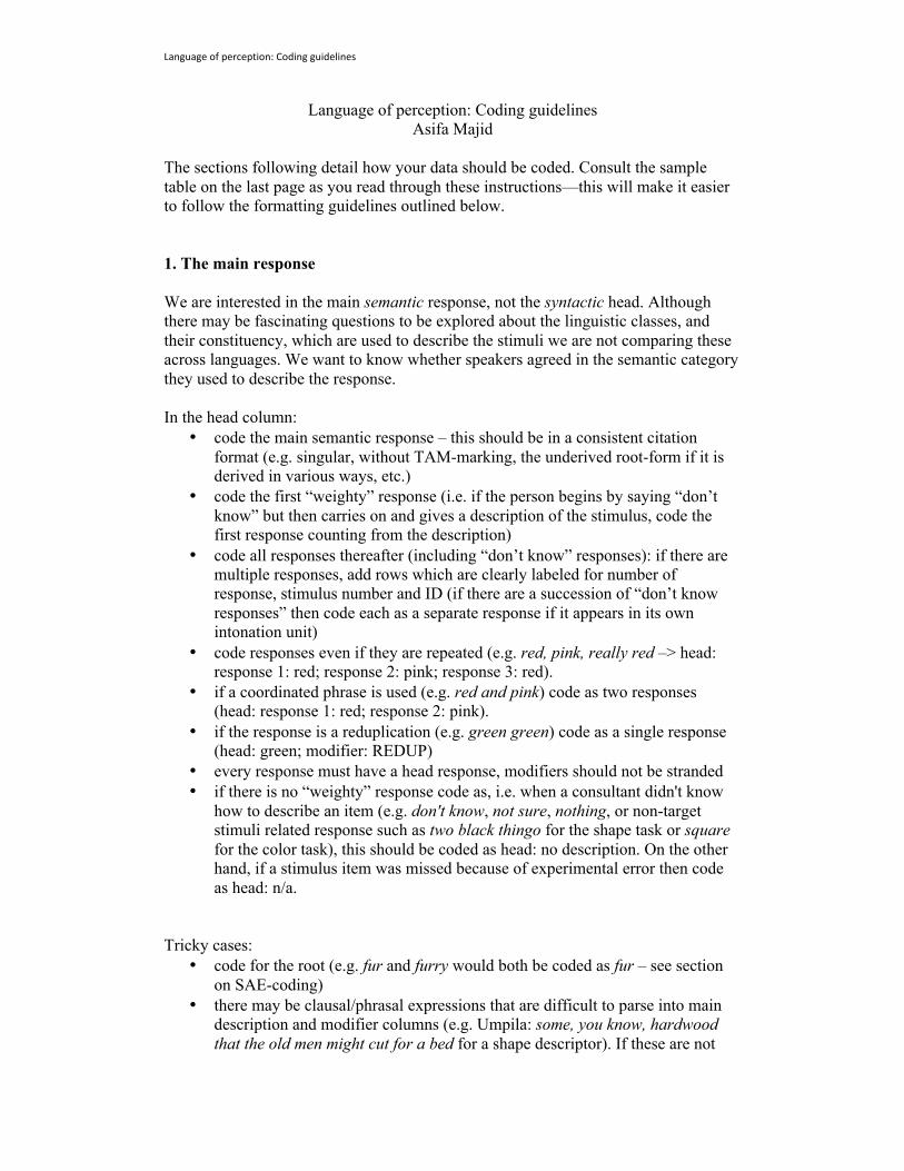
The outliers in the bottom left of the plot (where the two measures disagree) come from cases where thereare many “no description” responses. e.g. colour 10G 8/6 for Umpila:ax = a[a$Language=="Umpila" & a$Stimulus.code=="colour.10G 8/6" &
a$Response==1,]table(ax$head)
#### kawithaman no description paachala## 1 9 1tx = ax[ax$head!="no description",]$head
The original measures remove “no description” responses. That means that the example above above yeilds aSimpson index of 0 - there is no agreement between the two speakers who responded. The Shannon indexis 0.6931472, since there are only two responses, and the Shannon index measures the information in thatsequence. Had there been 14 completely different responses, then the Shannon index would be 2.64, which iscloser to the simple relationship.
One solution is to count “no description” responses as unique labels. So in the example above, the table ofresponses would be:tx.nd = ax$headtx.nd[tx.nd=='no description'] =
paste0("R",1:sum(tx.nd=="no description"))tx.nd
## [1] "R1" "R2" "paachala" "R3" "R4"## [6] "R5" "R6" "kawithaman" "R7" "R8"## [11] "R9"
This does not affect the Simpson index, but raises the Shannon index to 2.4. It also has the advantage ofproducing a defined index for cases where no participants produced a label.
19

If we calculate all indices while counting “no description” responses as unique responses, then we get thefollowing relationship:plot(d.nd$shannon.diversityIndex,
d.nd$simpson.diversityIndex)
0.0 0.5 1.0 1.5 2.0 2.5
0.0
0.2
0.4
0.6
0.8
1.0
d.nd$shannon.diversityIndex
d.nd
$sim
pson
.div
ersi
tyIn
dex
cor.test(d.nd$shannon.diversityIndex,d.nd$simpson.diversityIndex)
#### Pearson's product-moment correlation#### data: d.nd$shannon.diversityIndex and d.nd$simpson.diversityIndex## t = -206.66, df = 2848, p-value < 2.2e-16## alternative hypothesis: true correlation is not equal to 0## 95 percent confidence interval:## -0.9704554 -0.9658590## sample estimates:## cor## -0.9682389# Proportion of values unchangedpvu = sum(d$simpson.diversityIndex ==
d.nd$simpson.diversityIndex[match(d$id, d.nd$id)]) / nrow(d)
63.17% of values are unchanged. The new values are also more highly correlated:nd.cor = summary(lm(simpson.diversityIndex~
shannon.diversityIndex +I(shannon.diversityIndex^2),
data = d.nd))nd.cor$r.squared
## [1] 0.9855785
20

Diversity and number of types
plot(d.nd$simpson.diversityIndex, d.nd$N)
0.0 0.2 0.4 0.6 0.8 1.0
24
68
1012
14
d.nd$simpson.diversityIndex
d.nd
$N
plot(d.nd$shannon.diversityIndex, d.nd$N)
0.0 0.5 1.0 1.5 2.0 2.5
24
68
1012
14
d.nd$shannon.diversityIndex
d.nd
$N
21

Brown and Lenneberg measure
The measure from Brown and Lenneberg (1954) of “interpersonal agreement” is caluclated as
CR-DR+20
Where, CR is the number of subjects who agree on the most common name and DR is the number of differentresponses a stimulus item receives (the +20 is so that the values remain positive). This does not adjust forthe number of participants/responses. Still, the values are very highly correlated with both Simpson andShannon indices, albeit non-linearly.plot(d.nd$shannon.diversityIndex,
d.nd$BnL.diversityIndex)
0.0 0.5 1.0 1.5 2.0 2.5
510
1520
2530
35
d.nd$shannon.diversityIndex
d.nd
$BnL
.div
ersi
tyIn
dex
cor.test(d.nd$shannon.diversityIndex,d.nd$BnL.diversityIndex)
#### Pearson's product-moment correlation#### data: d.nd$shannon.diversityIndex and d.nd$BnL.diversityIndex## t = -272.42, df = 2848, p-value < 2.2e-16## alternative hypothesis: true correlation is not equal to 0## 95 percent confidence interval:## -0.9826563 -0.9799387## sample estimates:## cor## -0.9813465plot(d.nd$simpson.diversityIndex,
d.nd$BnL.diversityIndex)
22

0.0 0.2 0.4 0.6 0.8 1.0
510
1520
2530
35
d.nd$simpson.diversityIndex
d.nd
$BnL
.div
ersi
tyIn
dex
cor.test(d.nd$simpson.diversityIndex,d.nd$BnL.diversityIndex)
#### Pearson's product-moment correlation#### data: d.nd$simpson.diversityIndex and d.nd$BnL.diversityIndex## t = 166.92, df = 2848, p-value < 2.2e-16## alternative hypothesis: true correlation is not equal to 0## 95 percent confidence interval:## 0.9489745 0.9557929## sample estimates:## cor## 0.9525029
In particular, the correlation with the Shannon index makes sense, because it is related to the ‘surprisal’ ofencountering a label that is not your own. However, this measure is not theoretically motivated, so the othertwo are preferred.
23

S4: Codability across languages and domains
24

Codability across languages and domains
ContentsIntroduction 25
Data . . . . . . . . . . . . . . . . . . . . . . . . . . . . . . . . . . . . . . . . . . . . . . . . . . . . . 25
Load libraries 26
Load data 26
Plot data 27
Run models 31Summary . . . . . . . . . . . . . . . . . . . . . . . . . . . . . . . . . . . . . . . . . . . . . . . . . . 38
Distribution assumpsions 39
Differences between domains 40
Differences between langauges 42
Description types and codability 45Permutation test . . . . . . . . . . . . . . . . . . . . . . . . . . . . . . . . . . . . . . . . . . . . . . 47
Stimulus set size 52
Description lengths 53
Introduction
This document provides R code for reproducing the test of the relative codability of the senses. We use mixedeffects modelling to test the influence of language and domain. The full model included random intercepts forstimulus, domain, language, and the interaction between language and domain. Log-likelihood comparisonwas used to compare the full model to a model without one of those intercepts
Data
The main data comes from ../data/DiversityIndices_ND.csv, which includes the Simpson’s diversityindex, counting no-responses as unique responses. Each row lists the codability of a particular stimulus for aparticular community. The variables are:
• Language: Language/Community name• domain: Sense domain• Stimulus.code: Identity of the stimulus• simpson.diversityIndex: Simpson’s diversity index• shannon.diversityIndex: Shannon diversity index• N: Number of responses• BnL.diversityIndex: Brown & Lenneberg diversity index• mean.number.of.words: Mean number of words in full response
25

Load libraries
library(lme4)library(sjPlot)library(REEMtree)library(ggplot2)library(party)library(reshape2)library(rpart.plot)library(lattice)library(dplyr)library(mgcv)library(lmtest)library(itsadug)
Load data
d = read.csv("../data/DiversityIndices_ND.csv", stringsAsFactors = F)
d = d[!is.na(d$simpson.diversityIndex),]
d$Language= as.factor(d$Language)d$domain = factor(d$domain, levels=c("colour",'shape','sound','touch','taste','smell'))
Get log of diversity index, (add 0.1 to avoid infinite values)d$logDiversity = log(d$simpson.diversityIndex+0.1)
Distribution is not very normal, but it’s difficult to approximate this distribution anyway.hist(d$logDiversity)
26

Histogram of d$logDiversity
d$logDiversity
Fre
quen
cy
−2.5 −2.0 −1.5 −1.0 −0.5 0.0
050
100
150
200
250
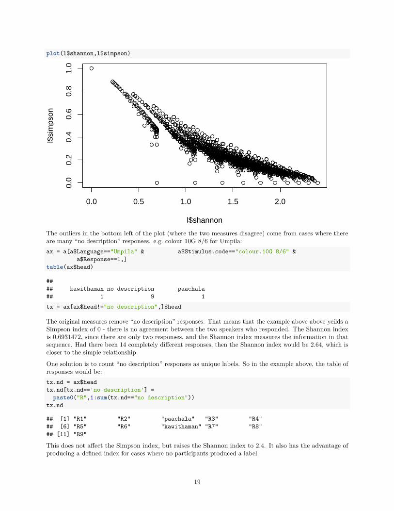
Plot data
g = ggplot(d, aes(y=simpson.diversityIndex, x=domain))g + geom_boxplot()
27

0.00
0.25
0.50
0.75
1.00
colour shape sound touch taste smell
domain
sim
pson
.div
ersi
tyIn
dex
g + geom_violin()
28

0.00
0.25
0.50
0.75
1.00
colour shape sound touch taste smell
domain
sim
pson
.div
ersi
tyIn
dex
g = ggplot(d, aes(y=shannon.diversityIndex, x=domain))g + geom_boxplot()
29

0
1
2
colour shape sound touch taste smell
domain
shan
non.
dive
rsity
Inde
x
g + geom_violin()
30
0
1
2
colour shape sound touch taste smell
domain
shan
non.
dive
rsity
Inde
x
Run models
m.full = lmer( logDiversity ~ 1 +(1|Language) +(1|domain/Stimulus.code) +(1|Language:domain),
data=d)
m.noL = lmer( logDiversity ~ 1 +(1|domain/Stimulus.code) +(1|Language:domain),
data=d)
m.noDom = lmer( logDiversity ~ 1 +(1|Language) +(1|Stimulus.code) +(1|Language:domain),
data=d)
m.noStim = lmer( logDiversity ~ 1 +(1|Language) +(1|domain) +(1|Language:domain),
data=d)
31

m.noLxD = lmer( logDiversity ~ 1 +(1|Language) +(1|domain/Stimulus.code),
data=d)
Test models:anova(m.full, m.noL)
## refitting model(s) with ML (instead of REML)
## Data: d## Models:## m.noL: logDiversity ~ 1 + (1 | domain/Stimulus.code) + (1 | Language:domain)## m.full: logDiversity ~ 1 + (1 | Language) + (1 | domain/Stimulus.code) +## m.full: (1 | Language:domain)## Df AIC BIC logLik deviance Chisq Chi Df Pr(>Chisq)## m.noL 5 3941.9 3971.6 -1965.9 3931.9## m.full 6 3939.3 3975.0 -1963.7 3927.3 4.5491 1 0.03294 *## ---## Signif. codes: 0 '***' 0.001 '**' 0.01 '*' 0.05 '.' 0.1 ' ' 1anova(m.full, m.noDom)
## refitting model(s) with ML (instead of REML)
## Data: d## Models:## m.noDom: logDiversity ~ 1 + (1 | Language) + (1 | Stimulus.code) + (1 |## m.noDom: Language:domain)## m.full: logDiversity ~ 1 + (1 | Language) + (1 | domain/Stimulus.code) +## m.full: (1 | Language:domain)## Df AIC BIC logLik deviance Chisq Chi Df Pr(>Chisq)## m.noDom 5 3965.1 3994.9 -1977.6 3955.1## m.full 6 3939.3 3975.0 -1963.7 3927.3 27.827 1 1.326e-07 ***## ---## Signif. codes: 0 '***' 0.001 '**' 0.01 '*' 0.05 '.' 0.1 ' ' 1anova(m.full, m.noStim)
## refitting model(s) with ML (instead of REML)
## Data: d## Models:## m.noStim: logDiversity ~ 1 + (1 | Language) + (1 | domain) + (1 | Language:domain)## m.full: logDiversity ~ 1 + (1 | Language) + (1 | domain/Stimulus.code) +## m.full: (1 | Language:domain)## Df AIC BIC logLik deviance Chisq Chi Df Pr(>Chisq)## m.noStim 5 4452.1 4481.9 -2221.1 4442.1## m.full 6 3939.3 3975.0 -1963.7 3927.3 514.81 1 < 2.2e-16 ***## ---## Signif. codes: 0 '***' 0.001 '**' 0.01 '*' 0.05 '.' 0.1 ' ' 1anova(m.full, m.noLxD)
## refitting model(s) with ML (instead of REML)
## Data: d## Models:
32
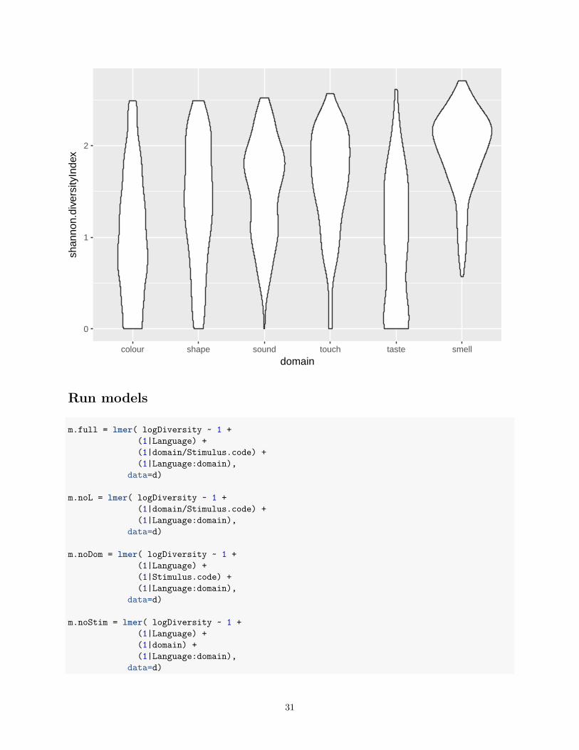
## m.noLxD: logDiversity ~ 1 + (1 | Language) + (1 | domain/Stimulus.code)## m.full: logDiversity ~ 1 + (1 | Language) + (1 | domain/Stimulus.code) +## m.full: (1 | Language:domain)## Df AIC BIC logLik deviance Chisq Chi Df Pr(>Chisq)## m.noLxD 5 4637.3 4667.1 -2313.7 4627.3## m.full 6 3939.3 3975.0 -1963.7 3927.3 700.03 1 < 2.2e-16 ***## ---## Signif. codes: 0 '***' 0.001 '**' 0.01 '*' 0.05 '.' 0.1 ' ' 1
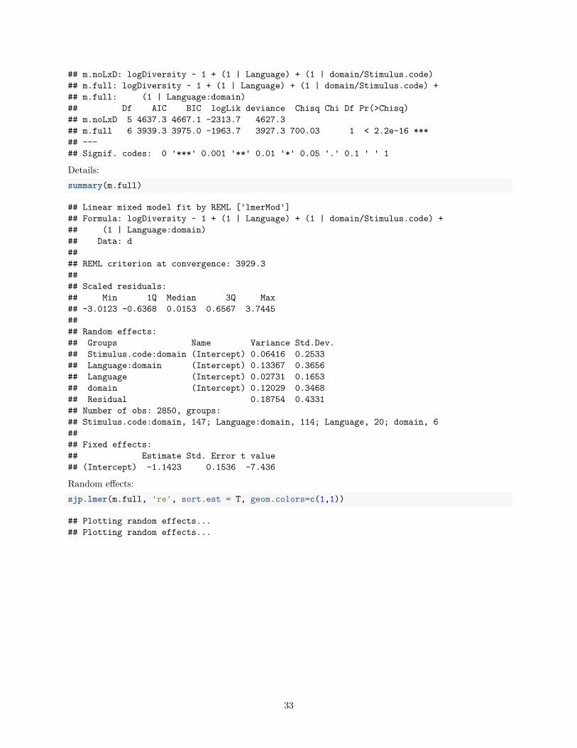
Details:summary(m.full)
## Linear mixed model fit by REML ['lmerMod']## Formula: logDiversity ~ 1 + (1 | Language) + (1 | domain/Stimulus.code) +## (1 | Language:domain)## Data: d#### REML criterion at convergence: 3929.3#### Scaled residuals:## Min 1Q Median 3Q Max## -3.0123 -0.6368 0.0153 0.6567 3.7445#### Random effects:## Groups Name Variance Std.Dev.## Stimulus.code:domain (Intercept) 0.06416 0.2533## Language:domain (Intercept) 0.13367 0.3656## Language (Intercept) 0.02731 0.1653## domain (Intercept) 0.12029 0.3468## Residual 0.18754 0.4331## Number of obs: 2850, groups:## Stimulus.code:domain, 147; Language:domain, 114; Language, 20; domain, 6#### Fixed effects:## Estimate Std. Error t value## (Intercept) -1.1423 0.1536 -7.436
Random effects:sjp.lmer(m.full, 're', sort.est = T, geom.colors=c(1,1))
## Plotting random effects...## Plotting random effects...
33

−0.60−0.52−0.49−0.47−0.47−0.46−0.45−0.44−0.42−0.41−0.37−0.30−0.28−0.28−0.27−0.27−0.26−0.26−0.25−0.25−0.25−0.25−0.24−0.23−0.23−0.23−0.22−0.22−0.21−0.21−0.20−0.17−0.16−0.16−0.16−0.16−0.15−0.15−0.15−0.14−0.14−0.13−0.12−0.11−0.11−0.11−0.10−0.10−0.10−0.10−0.09−0.08−0.07−0.07−0.06−0.06−0.06−0.05−0.05−0.05−0.04−0.04−0.03−0.03−0.03−0.02−0.02−0.02−0.02−0.01−0.000.010.020.020.020.020.030.030.030.040.050.050.050.050.050.060.060.060.070.070.070.070.080.080.080.090.090.090.100.110.110.110.120.120.130.140.140.140.150.150.150.150.160.170.170.180.180.190.190.200.200.200.210.210.210.220.220.220.220.230.240.260.270.290.300.330.330.350.380.400.400.400.460.490.510.540.67(Intercept)
−0.5 0.0 0.5sound.sound.tempo.4b:soundcolour.5R 2/8:colourcolour.5Y 4/6:coloursound.sound.tempo.7a:soundsound.sound.tempo.7b:soundcolour.10R 8/6:colourcolour.10RP 2/8:colourcolour.5Y 6/10:colourcolour.5R 8/6:coloursound.sound.tempo.4a:soundshape.flower:shapecolour.10YR 4/8:colourcolour.10RP 8/6:colourcolour.5YR 8/8:colourcolour.5P 6/8:colourshape.cone:shapesmell.smoke:smellshape.cylinder:shapecolour.5RP 2/8:colourcolour.10YR 6/12:colourshape.3 cones:shapecolour.10P 2/6:colourtaste.glutamate (umami):tastecolour.5YR 4/8:colourcolour.10P 6/10:colourcolour.10PB 6/10:colourcolour.10PB 4/12:colourtouch.curved ridges (wide spacing):touchtouch.beads:touchcolour.5YR 2/4:colourtouch.straight ridges (small spacing):touchcolour.10Y 6/10:colourcolour.10BG 8/4:colourcolour.10BG 4/6:coloursmell.lemon:smellcolour.5RP 4/12:colourshape.elipsoid:shapesmell.gasoline:smelltouch.cork:touchcolour.5P 2/8:colourcolour.10R 2/6:colourcolour.10BG 6/8:colourcolour.5B 2/6:colourcolour.5P 8/4:colourcolour.10P 4/12:coloursmell.paint thinner:smellcolour.5GY 8/10:colourcolour.5GY 2/2:colourshape.2 triangles:shapecolour.5BG 8/4:colourcolour.5P 4/12:colourshape.rectangle 3D:shapecolour.10P 8/6:colourcolour.10Y 4/6:colourcolour.5RP 8/6:coloursound.sound.loud−up.1a:soundshape.sphere:shapesmell.turpentine:smellcolour.10R 4/12:colourcolour.10PB 2/10:colourcolour.5B 8/4:colourshape.cube:shapeshape.2 spheres:shapesmell.onion:smellcolour.10BG 2/6:coloursmell.chocolate:smellcolour.5PB 8/6:colourcolour.10YR 2/2:colourcolour.5R 6/12:colourtouch.felt:touchshape.rectangle:shapesound.sound.pitch−up.2a:soundcolour.10GY 2/4:colourcolour.5YR 6/14:colourcolour.10B 8/6:coloursmell.soap:smellshape.2 cubes:shapetaste.citric acide monohydrate (sour):tastesmell.pineapple:smellcolour.10PB 8/4:coloursound.sound.pitch−down.8a:soundsound.sound.loud−down.6a:soundtaste.quinine hydrochloride (bitter):tastecolour.5B 4/10:colourcolour.5B 6/10:colourcolour.10R 6/14:coloursmell.rose:smellsound.sound.loud−down.3b:soundcolour.5PB 6/10:colourcolour.5PB 2/8:colourshape.3 squares:shapesound.sound.pitch−down.5a:soundshape.elipse:shapesmell.banana:smelltouch.feather:touchtouch.fur (synthetic):touchshape.triangle:shapesound.sound.loud−up.10b:soundsound.sound.pitch−down.8b:soundcolour.5RP 6/12:colourcolour.10G 2/6:colourcolour.5BG 6/10:colourcolour.5BG 2/6:coloursound.sound.loud−up.10a:soundshape.3 elipses:shapecolour.10B 2/6:colourcolour.10B 6/10:coloursound.sound.loud−down.6b:soundtouch.jagged (fabric):touchcolour.5Y 2/2:colourtaste.sodium chloride (salt):tastesound.sound.loud−up.1b:soundcolour.5G 2/6:colourshape.2 circles:shapeshape.square:shapecolour.10Y 8/12:colourtouch.plastic (sheet):touchcolour.5GY 4/8:coloursound.sound.pitch−up.9b:soundsound.sound.pitch−up.2b:soundcolour.10RP 6/12:coloursound.sound.pitch−up.9a:soundcolour.10YR 8/14:colourcolour.10B 4/10:colourtouch.rubber (yoga mat):touchsound.sound.pitch−down.5b:soundcolour.10G 8/6:colourtaste.sucrose (sweet):tastecolour.5BG 4/8:colourshape.circle:shapecolour.5G 8/6:colourcolour.10Y 2/2:colourcolour.5PB 4/12:coloursound.sound.loud−down.3a:soundcolour.10RP 4/14:coloursmell.cinnamon:smellcolour.10GY 8/8:colourcolour.5GY 6/10:colourcolour.10G 6/10:colourcolour.5G 6/10:colourcolour.10GY 4/8:colourcolour.5Y 8/14:colourcolour.5G 4/10:colourcolour.10GY 6/12:colourcolour.10G 4/10:colourcolour.5R 4/14:colourshape.star:shape
BLUP
Gro
up le
vels
## Plotting random effects...
34

−0.83−0.76−0.67−0.65−0.61−0.53−0.50−0.50−0.45−0.44−0.44−0.41−0.37−0.37−0.36−0.34−0.33−0.33−0.32−0.29−0.29−0.26−0.25−0.24−0.24−0.22−0.21−0.21−0.21−0.20−0.20−0.20−0.19−0.19−0.17−0.16−0.15−0.15−0.15−0.13−0.12−0.11−0.11−0.11−0.10−0.10−0.09−0.09−0.07−0.05−0.05−0.05−0.04−0.03−0.03−0.03−0.02−0.020.000.000.010.010.020.030.040.050.050.050.060.090.110.110.120.130.130.130.130.150.160.180.190.200.220.230.230.240.240.240.250.260.280.290.290.300.310.330.330.330.380.380.380.400.420.460.470.480.480.480.500.520.580.650.750.85(Intercept)
−1.0 −0.5 0.0 0.5 1.0Dogul Dom:shapeUmpila:colourKata Kolok:colourUmpila:shapeBSL:tasteTzeltal:shapeFarsi:soundSiwu:soundASL:tasteASL:touchYeli Dnye:shapeYeli Dnye:colourKilivila:colourKilivila:soundCantonese:smellKata Kolok:touchEnglish:tasteZapotec:smellTurkish:touchBSL:touchCantonese:touchUmpila:tasteSiwu:colourYucatec:touchMalay:tasteASL:smellTzeltal:smellEnglish:touchMian:smellFarsi:touchYurakare:shapeEnglish:smellYurakare:smellMian:soundYeli Dnye:soundSiwu:shapeMalay:smellLao:colourBSL:smellYucatec:smellSemai:smellSemai:colourUmpila:touchMalay:soundYurakare:colourKilivila:smellKata Kolok:shapeUmpila:soundSemai:shapeMian:shapeSiwu:tasteLao:soundYurakare:touchKata Kolok:tasteSemai:touchZapotec:shapeDogul Dom:soundFarsi:smellDogul Dom:tasteYeli Dnye:tasteLao:shapeKilivila:touchTurkish:colourMalay:touchTurkish:smellDogul Dom:smellKilivila:shapeYeli Dnye:smellBSL:shapeYurakare:tasteKata Kolok:smellKilivila:tasteZapotec:soundTzeltal:touchDogul Dom:colourZapotec:touchLao:touchSemai:soundZapotec:tasteZapotec:colourTurkish:tasteMian:touchMian:colourTzeltal:colourEnglish:soundYucatec:tasteFarsi:colourSiwu:smellYucatec:colourCantonese:soundCantonese:colourYucatec:shapeCantonese:tasteFarsi:shapeEnglish:colourMalay:colourYeli Dnye:touchTzeltal:soundTurkish:shapeTzeltal:tasteYucatec:soundTurkish:soundEnglish:shapeFarsi:tasteBSL:colourASL:shapeLao:smellLao:tasteASL:colourCantonese:shapeMalay:shapeSiwu:touchDogul Dom:touchUmpila:smell
BLUP
Gro
up le
vels
## Plotting random effects...
35

−0.21−0.21
−0.14−0.13
−0.10−0.09
−0.04−0.03−0.02−0.00
0.010.050.050.060.07
0.090.140.14
0.160.19
(Intercept)
−0.25 0.00 0.25
Kata Kolok
Umpila
Kilivila
Yeli Dnye
BSL
Yurakare
Semai
ASL
Siwu
Mian
Dogul Dom
English
Zapotec
Farsi
Tzeltal
Malay
Cantonese
Turkish
Yucatec
Lao
BLUP
Gro
up le
vels
−0.50
−0.14
−0.11
0.05
0.32
0.39
(Intercept)
−0.4 0.0 0.4
smell
touch
sound
shape
colour
taste
BLUP
Gro
up le
vels
36

plot(predict(m.full), d$simpson.diversityIndex)
−2.0 −1.5 −1.0 −0.5 0.0
0.0
0.2
0.4
0.6
0.8
1.0
predict(m.full)
d$si
mps
on.d
iver
sity
Inde
x
37
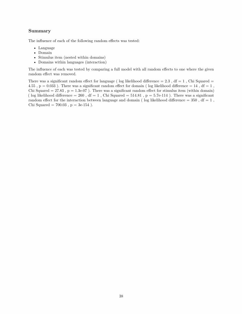
Summary
The influence of each of the following random effects was tested:
• Language• Domain• Stimulus item (nested within domains)• Domains within languages (interaction)
The influence of each was tested by comparing a full model with all random effects to one where the givenrandom effect was removed.
There was a significant random effect for language ( log likelihood difference = 2.3 , df = 1 , Chi Squared =4.55 , p = 0.033 ). There was a significant random effect for domain ( log likelihood difference = 14 , df = 1 ,Chi Squared = 27.83 , p = 1.3e-07 ). There was a significant random effect for stimulus item (within domain)( log likelihood difference = 260 , df = 1 , Chi Squared = 514.81 , p = 5.7e-114 ). There was a significantrandom effect for the interaction between language and domain ( log likelihood difference = 350 , df = 1 ,Chi Squared = 700.03 , p = 3e-154 ).
38

Distribution assumpsions
The fit of the model distributions is reasonable:par(mfrow=c(1,2))hist(predict(m.full), main="Model predicitons")hist(d$logDiversity, main="Actual data")
Model predicitons
predict(m.full)
Fre
quen
cy
−2.5 −1.5 −0.5 0.5
010
020
030
040
0
Actual data
d$logDiversity
Fre
quen
cy
−2.5 −1.5 −0.5
050
100
150
200
250
We can try fitting the data with different distributions (Gamma, inverse gaussian):
The gaussian model is the best fit by AIC.
39

Differences between domains
How do the different domains cluster according to codability? We can use REEMtree which allows randomeffects for Language and Stimulus:REEMresult<-REEMtree(simpson.diversityIndex~ domain,
data=d,random= list(~ 1|Language,~1|Stimulus.code),MaxIterations = 100000)
rpart.plot(tree(REEMresult), type=3)
domain = shape,sound,touch,smell
domain = smell
colour,taste
shape,sound,touch
0.118%
0.2732%
0.4559%
rtrf.lang = REEMresult$RandomEffects$Languagertrf.lang.intercept = rtrf.lang[,1]names(rtrf.lang.intercept) = rownames(rtrf.lang)dotplot(sort(rtrf.lang.intercept))
40

sort(rtrf.lang.intercept)
Kata KolokUmpilaKilivila
Yeli DnyeYurakare
SemaiSiwu
Dogul DomMianLao
ZapotecBSL
FarsiTzeltalTurkishEnglish
MalayYucatec
ASLCantonese
−0.2 −0.1 0.0 0.1
According to the decision tree results, the hierarchy of codability is:
[Colour, Taste] > [Shape, Sound, Touch] > Smell
41

Differences between langauges
We can also ask which languages cluster together:d$L = substr(d$Language,1,3)REEMresult.lang<-REEMtree(simpson.diversityIndex~ L,
data=d,random= c(~ 1|domain,~1|Stimulus.code),MaxIterations = 100000)
rpart.plot(tree(REEMresult.lang), type=4, extra=100,box.palette="RdYlGn")
L = Kat,Kil,Sem,Siw,Ump,Yel,Yur
L = Kat,Kil,Ump L = BSL,Dog,Far,Lao,Mia,Tur,Tze,Zap
ASL,BSL,Can,Dog,Eng,Far,Lao,Mal,Mia,Tur,Tze,Yuc,Zap
Sem,Siw,Yel,Yur ASL,Can,Eng,Mal,Yuc
0.31100%
0.1535%
0.08615%
0.2120%
0.3965%
0.3540%
0.4425%
rtrf.dom = REEMresult.lang$RandomEffects$domainrtrf.dom.intercept = rtrf.dom[,1]names(rtrf.dom.intercept) = rownames(rtrf.dom)dotplot(sort(rtrf.dom.intercept))
42

sort(rtrf.dom.intercept)
smell
touch
sound
shape
colour
taste
−0.2 −0.1 0.0 0.1
Here’s a decision tree splitting the data by domain and language. It is harder to understand the splits here,which is to say that it is not easy to make a generalisation about the differences. The main point is thatthere are many interactions between langauge and domain, not just one big difference.REEMresult.both<-REEMtree(simpson.diversityIndex~ L+domain,
data=d,random= ~ 1|Stimulus.code,MaxIterations = 100000)
rpart.plot(tree(REEMresult.both), type=4, extra=100,box.palette="RdYlGn")
L = Kat,Kil,Sem,Siw,Ump,Yel,Yur
L = Kat,Kil,Ump,Yel
L = Kat,Ump
domain = sound,smell
domain = shape,sound,smell
domain = shape,sound,touch,smell
domain = touch,smell
L = ASL,BSL,Can,Eng,Far,Mal,Mia,Tur,Tze,Yuc,Zap L = BSL,Dog,Far,Lao,Mia,Tze,Zap
L = Dog,Mia domain = sound
L = Dog,Lao,Mia,Tur,Zap
domain = taste
L = ASL,BSL,Eng,Mal
ASL,BSL,Can,Dog,Eng,Far,Lao,Mal,Mia,Tur,Tze,Yuc,Zap
Sem,Siw,Yur
Kil,Yel
colour,shape,touch,taste
colour,touch,taste
colour,taste
shape,sound
Dog,Lao ASL,Can,Eng,Mal,Tur,Yuc
BSL,Far,Lao,Tze,Zap shape
ASL,BSL,Can,Eng,Far,Mal,Tze,Yuc
colour
Can,Far,Tze,Yuc
0.37100%
0.2135%
0.1620%
0.1310%
0.210%
0.112%
0.238%
0.2815%
0.195%
0.3310%
0.4465%
0.2927%
0.1910%
0.148%
0.352%
0.3517%
0.249%
0.173%
0.286%
0.478%
0.384%
0.564%
0.5539%
0.4815%
0.624%
0.421%
0.0851%
0.651%
0.6122%
pdf("../results/graphs/DecisionTree_LanguagesAndDomains.pdf",width=15, height=10)
rpart.plot(tree(REEMresult.both), type=4, extra=100,box.palette="RdYlGn")
dev.off()
43

## 2tree(REEMresult.both)$variable.importance
## L domain## 53.49488 40.98518
We were also interested in whether languages differ by modality:d$L = substr(d$Language,1,3)d$modality = "Spoken"d$modality[d$Language %in% c("ASL", "BSL", "Kata Kolok")] = "Signed"REEMresult.mod<-REEMtree(simpson.diversityIndex~ L + domain + modality,
data=d,random= c(~1|Stimulus.code),MaxIterations = 100000)
tree(REEMresult.mod)$variable.importance
## L domain modality## 56.952422 42.103148 2.010103
Modality is not used in the tree (not shown), and is not used if it is the only variable in available to the tree(not shown). The importance measure for modality is 20 times lower than for language and domain. That is,languages do not cluster by modality.
44
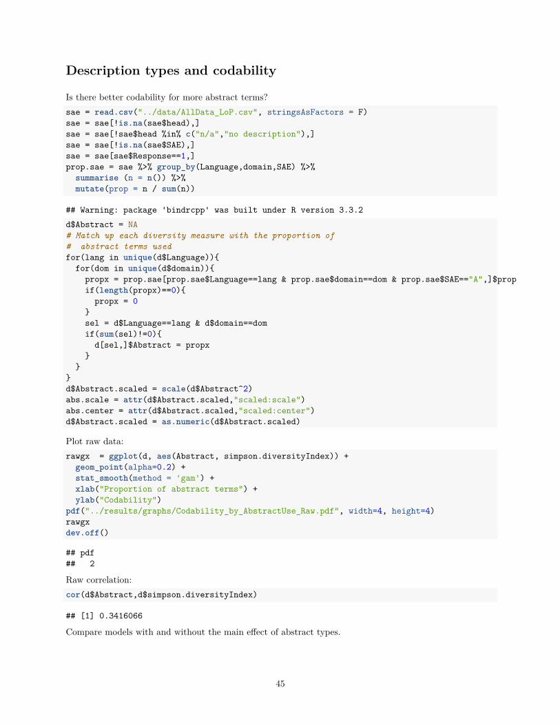
Description types and codability
Is there better codability for more abstract terms?sae = read.csv("../data/AllData_LoP.csv", stringsAsFactors = F)sae = sae[!is.na(sae$head),]sae = sae[!sae$head %in% c("n/a","no description"),]sae = sae[!is.na(sae$SAE),]sae = sae[sae$Response==1,]prop.sae = sae %>% group_by(Language,domain,SAE) %>%
summarise (n = n()) %>%mutate(prop = n / sum(n))
## Warning: package 'bindrcpp' was built under R version 3.3.2d$Abstract = NA# Match up each diversity measure with the proportion of# abstract terms usedfor(lang in unique(d$Language)){
for(dom in unique(d$domain)){propx = prop.sae[prop.sae$Language==lang & prop.sae$domain==dom & prop.sae$SAE=="A",]$propif(length(propx)==0){
propx = 0}sel = d$Language==lang & d$domain==domif(sum(sel)!=0){
d[sel,]$Abstract = propx}
}}d$Abstract.scaled = scale(d$Abstract^2)abs.scale = attr(d$Abstract.scaled,"scaled:scale")abs.center = attr(d$Abstract.scaled,"scaled:center")d$Abstract.scaled = as.numeric(d$Abstract.scaled)
Plot raw data:rawgx = ggplot(d, aes(Abstract, simpson.diversityIndex)) +
geom_point(alpha=0.2) +stat_smooth(method = 'gam') +xlab("Proportion of abstract terms") +ylab("Codability")
pdf("../results/graphs/Codability_by_AbstractUse_Raw.pdf", width=4, height=4)rawgxdev.off()
## pdf## 2
Raw correlation:cor(d$Abstract,d$simpson.diversityIndex)
## [1] 0.3416066
Compare models with and without the main effect of abstract types.
45

m0.sae = lmer( logDiversity ~ 1 +(1+Abstract.scaled|Language) +(1+Abstract.scaled|domain/Stimulus.code) +(1|Language:domain),
data=d)
m1.sae = update(m0.sae, ~.+Abstract.scaled)anova(m0.sae,m1.sae)
## refitting model(s) with ML (instead of REML)
## Data: d## Models:## m0.sae: logDiversity ~ 1 + (1 + Abstract.scaled | Language) + (1 + Abstract.scaled |## m0.sae: domain/Stimulus.code) + (1 | Language:domain)## m1.sae: logDiversity ~ (1 + Abstract.scaled | Language) + (1 + Abstract.scaled |## m1.sae: domain/Stimulus.code) + (1 | Language:domain) + Abstract.scaled## Df AIC BIC logLik deviance Chisq Chi Df Pr(>Chisq)## m0.sae 12 3871.3 3942.8 -1923.7 3847.3## m1.sae 13 3858.3 3935.7 -1916.1 3832.3 15.009 1 0.000107 ***## ---## Signif. codes: 0 '***' 0.001 '**' 0.01 '*' 0.05 '.' 0.1 ' ' 1px = sjp.lmer(m1.sae,'eff','Abstract.scaled', show.ci = T, prnt.plot = F)px$plot$data$x = sqrt((px$plot$data$x * abs.scale + abs.center))px$plot$data$y = exp(px$plot$data$y) -0.1px$plot$data$upper = exp(px$plot$data$upper) -0.1px$plot$data$lower = exp(px$plot$data$lower) -0.1px = px$plot+ xlab("Proportion of abstract terms") +
ylab("Codability") +theme(strip.background = element_blank(),
strip.text.y = element_blank(),plot.title = element_blank())
pdf("../results/graphs/Codability_by_AbstractUse.pdf", width=4, height=4)pxdev.off()
## pdf## 2save(px,file="../results/graphs/Codability_by_AbstractUse_ggplot.RDat")
46
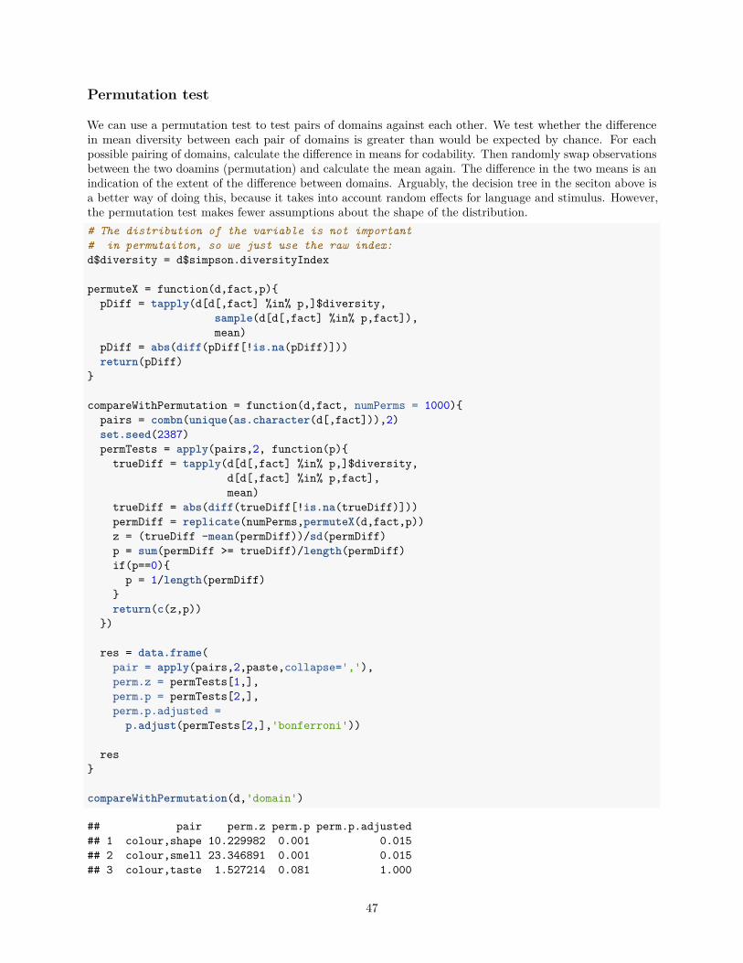
Permutation test
We can use a permutation test to test pairs of domains against each other. We test whether the differencein mean diversity between each pair of domains is greater than would be expected by chance. For eachpossible pairing of domains, calculate the difference in means for codability. Then randomly swap observationsbetween the two doamins (permutation) and calculate the mean again. The difference in the two means is anindication of the extent of the difference between domains. Arguably, the decision tree in the seciton above isa better way of doing this, because it takes into account random effects for language and stimulus. However,the permutation test makes fewer assumptions about the shape of the distribution.# The distribution of the variable is not important# in permutaiton, so we just use the raw index:d$diversity = d$simpson.diversityIndex
permuteX = function(d,fact,p){pDiff = tapply(d[d[,fact] %in% p,]$diversity,
sample(d[d[,fact] %in% p,fact]),mean)
pDiff = abs(diff(pDiff[!is.na(pDiff)]))return(pDiff)
}
compareWithPermutation = function(d,fact, numPerms = 1000){pairs = combn(unique(as.character(d[,fact])),2)set.seed(2387)permTests = apply(pairs,2, function(p){
trueDiff = tapply(d[d[,fact] %in% p,]$diversity,d[d[,fact] %in% p,fact],mean)
trueDiff = abs(diff(trueDiff[!is.na(trueDiff)]))permDiff = replicate(numPerms,permuteX(d,fact,p))z = (trueDiff -mean(permDiff))/sd(permDiff)p = sum(permDiff >= trueDiff)/length(permDiff)if(p==0){
p = 1/length(permDiff)}return(c(z,p))
})
res = data.frame(pair = apply(pairs,2,paste,collapse=','),perm.z = permTests[1,],perm.p = permTests[2,],perm.p.adjusted =
p.adjust(permTests[2,],'bonferroni'))
res}
compareWithPermutation(d,'domain')
## pair perm.z perm.p perm.p.adjusted## 1 colour,shape 10.229982 0.001 0.015## 2 colour,smell 23.346891 0.001 0.015## 3 colour,taste 1.527214 0.081 1.000
47

## 4 colour,touch 14.925907 0.001 0.015## 5 colour,sound 16.716660 0.001 0.015## 6 shape,smell 15.457834 0.001 0.015## 7 shape,taste 7.292646 0.001 0.015## 8 shape,touch 6.009034 0.001 0.015## 9 shape,sound 5.685990 0.001 0.015## 10 smell,taste 17.711571 0.001 0.015## 11 smell,touch 9.603543 0.001 0.015## 12 smell,sound 12.351339 0.001 0.015## 13 taste,touch 11.245055 0.001 0.015## 14 taste,sound 12.567821 0.001 0.015## 15 touch,sound 0.463503 0.288 1.000
The mean codability for all paris of domains are different, except for:
• Colour and Taste• Touch and Sound
So, the hierarchy is:
[Colour, Taste] > Shape > [Sound, Touch] > Smell
Which matches the decision tree hierarchy very well.
Permutation between languages
Test whether the mean diversity differs between each pair of languages. This is just to double-check that theresults from the mixed effects model above are not artefacts of the shape of the codability distribution. Alarge number of permutations is needed so that the p-value remains significant when controlling for multiplecomparisons.d$Language2 = factor(d$Language,
levels =names(sort(
tapply(d$simpson.diversityIndex,d$Language,mean))))
ggplot(d, aes(y=diversity,x=Language2)) +geom_boxplot() + coord_flip()
48

Kata Kolok
Umpila
Kilivila
Yeli Dnye
Semai
Yurakare
Siwu
Dogul Dom
Mian
Lao
Zapotec
Farsi
Tzeltal
BSL
Turkish
English
Malay
Yucatec
Cantonese
ASL
0.00 0.25 0.50 0.75 1.00
diversity
Lang
uage
2
# (need 20000 permutations for Bonferroni correction)langPerm = compareWithPermutation(d,'Language', numPerms = 20000)
List of significant differences:langPerm[langPerm$perm.p.adjusted<0.01,]
## pair perm.z perm.p perm.p.adjusted## 3 ASL,Dogul Dom 6.386793 5e-05 0.0095## 6 ASL,Kata Kolok 14.415690 5e-05 0.0095## 7 ASL,Kilivila 13.020372 5e-05 0.0095## 8 ASL,Lao 5.119374 5e-05 0.0095## 10 ASL,Mian 4.755508 5e-05 0.0095## 11 ASL,Semai 10.017882 5e-05 0.0095## 12 ASL,Siwu 7.888725 5e-05 0.0095## 15 ASL,Umpila 14.872409 5e-05 0.0095## 16 ASL,Yeli Dnye 11.306146 5e-05 0.0095## 18 ASL,Yurakare 8.723735 5e-05 0.0095## 24 BSL,Kata Kolok 12.718123 5e-05 0.0095## 25 BSL,Kilivila 10.739672 5e-05 0.0095## 29 BSL,Semai 6.978705 5e-05 0.0095## 30 BSL,Siwu 4.778091 5e-05 0.0095## 33 BSL,Umpila 12.883928 5e-05 0.0095## 34 BSL,Yeli Dnye 8.647660 5e-05 0.0095## 36 BSL,Yurakare 5.794757 5e-05 0.0095## 38 Cantonese,Dogul Dom 7.019165 5e-05 0.0095## 41 Cantonese,Kata Kolok 15.741879 5e-05 0.0095## 42 Cantonese,Kilivila 14.306751 5e-05 0.0095
49

## 43 Cantonese,Lao 5.606992 5e-05 0.0095## 45 Cantonese,Mian 5.207652 5e-05 0.0095## 46 Cantonese,Semai 10.881228 5e-05 0.0095## 47 Cantonese,Siwu 8.545814 5e-05 0.0095## 50 Cantonese,Umpila 16.091613 5e-05 0.0095## 51 Cantonese,Yeli Dnye 12.195978 5e-05 0.0095## 53 Cantonese,Yurakare 9.526955 5e-05 0.0095## 54 Cantonese,Zapotec 4.934960 5e-05 0.0095## 57 Dogul Dom,Kata Kolok 11.168765 5e-05 0.0095## 58 Dogul Dom,Kilivila 8.305659 5e-05 0.0095## 60 Dogul Dom,Malay 5.805998 5e-05 0.0095## 66 Dogul Dom,Umpila 11.144685 5e-05 0.0095## 67 Dogul Dom,Yeli Dnye 5.845490 5e-05 0.0095## 68 Dogul Dom,Yucatec 6.578805 5e-05 0.0095## 72 English,Kata Kolok 14.261218 5e-05 0.0095## 73 English,Kilivila 12.595069 5e-05 0.0095## 77 English,Semai 8.608346 5e-05 0.0095## 78 English,Siwu 6.186397 5e-05 0.0095## 81 English,Umpila 14.512258 5e-05 0.0095## 82 English,Yeli Dnye 10.281170 5e-05 0.0095## 84 English,Yurakare 7.224110 5e-05 0.0095## 86 Farsi,Kata Kolok 12.842217 5e-05 0.0095## 87 Farsi,Kilivila 10.844462 5e-05 0.0095## 91 Farsi,Semai 6.809733 5e-05 0.0095## 95 Farsi,Umpila 13.043482 5e-05 0.0095## 96 Farsi,Yeli Dnye 8.778286 5e-05 0.0095## 98 Farsi,Yurakare 5.748382 5e-05 0.0095## 101 Kata Kolok,Lao 13.387166 5e-05 0.0095## 102 Kata Kolok,Malay 15.130729 5e-05 0.0095## 103 Kata Kolok,Mian 11.453272 5e-05 0.0095## 104 Kata Kolok,Semai 9.349440 5e-05 0.0095## 105 Kata Kolok,Siwu 7.786608 5e-05 0.0095## 106 Kata Kolok,Turkish 14.183490 5e-05 0.0095## 107 Kata Kolok,Tzeltal 12.948404 5e-05 0.0095## 110 Kata Kolok,Yucatec 16.100007 5e-05 0.0095## 111 Kata Kolok,Yurakare 7.727963 5e-05 0.0095## 112 Kata Kolok,Zapotec 12.986692 5e-05 0.0095## 113 Kilivila,Lao 10.455641 5e-05 0.0095## 114 Kilivila,Malay 13.540861 5e-05 0.0095## 115 Kilivila,Mian 8.856748 5e-05 0.0095## 116 Kilivila,Semai 4.971180 5e-05 0.0095## 118 Kilivila,Turkish 12.264060 5e-05 0.0095## 119 Kilivila,Tzeltal 11.005224 5e-05 0.0095## 122 Kilivila,Yucatec 14.469779 5e-05 0.0095## 124 Kilivila,Zapotec 10.455408 5e-05 0.0095## 127 Lao,Semai 5.647939 5e-05 0.0095## 131 Lao,Umpila 13.234881 5e-05 0.0095## 132 Lao,Yeli Dnye 7.753110 5e-05 0.0095## 133 Lao,Yucatec 5.017567 5e-05 0.0095## 137 Malay,Semai 9.956038 5e-05 0.0095## 138 Malay,Siwu 7.352764 5e-05 0.0095## 141 Malay,Umpila 15.483867 5e-05 0.0095## 142 Malay,Yeli Dnye 11.330134 5e-05 0.0095## 144 Malay,Yurakare 8.461861 5e-05 0.0095
50

## 150 Mian,Umpila 11.574841 5e-05 0.0095## 151 Mian,Yeli Dnye 6.770497 5e-05 0.0095## 156 Semai,Turkish 8.180076 5e-05 0.0095## 157 Semai,Tzeltal 7.038307 5e-05 0.0095## 158 Semai,Umpila 8.942022 5e-05 0.0095## 160 Semai,Yucatec 10.851852 5e-05 0.0095## 162 Semai,Zapotec 5.921801 5e-05 0.0095## 163 Siwu,Turkish 5.617457 5e-05 0.0095## 165 Siwu,Umpila 7.902980 5e-05 0.0095## 167 Siwu,Yucatec 8.138316 5e-05 0.0095## 171 Turkish,Umpila 14.392934 5e-05 0.0095## 172 Turkish,Yeli Dnye 9.926558 5e-05 0.0095## 174 Turkish,Yurakare 6.823549 5e-05 0.0095## 176 Tzeltal,Umpila 13.248762 5e-05 0.0095## 177 Tzeltal,Yeli Dnye 8.751177 5e-05 0.0095## 179 Tzeltal,Yurakare 5.780601 5e-05 0.0095## 182 Umpila,Yucatec 16.471421 5e-05 0.0095## 183 Umpila,Yurakare 7.599645 5e-05 0.0095## 184 Umpila,Zapotec 13.166837 5e-05 0.0095## 185 Yeli Dnye,Yucatec 12.207134 5e-05 0.0095## 187 Yeli Dnye,Zapotec 8.009367 5e-05 0.0095## 188 Yucatec,Yurakare 9.268163 5e-05 0.0095
Languages really are different, but some languages are closer than others. This heatmap gives an idea ofwhich languages are similar to which.d$Language2 = factor(d$Language, levels =
names(sort(tapply(d$diversity,d$Language,mean))))
langPerm$l1 = sapply(as.character(langPerm$pair), function(X){strsplit(X,',')[[1]][1]})langPerm$l2 = sapply(as.character(langPerm$pair), function(X){strsplit(X,',')[[1]][2]})
lxs = unique(d$Language)langPerm2 = langPermlangPerm2 = rbind(
langPerm,data.frame(
pair = paste(lxs,lxs,sep=','),perm.z = 0,perm.p = 1,perm.p.adjusted = 1,l1 = lxs,l2 = lxs
))
langPerm2$perm.z = abs(langPerm2$perm.z)
langPermDist = acast(langPerm2, l1~l2, value.var="perm.z")
langPermDist[lower.tri(langPermDist)] = t(langPermDist)[lower.tri(langPermDist)]
51

heatmap(langPermDist)
Yeli
Dny
eK
ilivi
laK
ata
Kol
okU
mpi
laS
emai
Siw
uYu
raka
reD
ogul
Dom
Mia
nZ
apot
ecLa
oE
nglis
hTu
rkis
hT
zelta
lB
SL
Fars
iM
alay
AS
LYu
cate
cC
anto
nese
Yeli DnyeKilivilaKata KolokUmpilaSemaiSiwuYurakareDogul DomMianZapotecLaoEnglishTurkishTzeltalBSLFarsiMalayASLYucatecCantonese
Stimulus set size
A check that the size of the stimulus set does not predict the codability:numStimuli = tapply(d$Stimulus.code,d$domain, function(X){length(unique(X))})
d$numStimuli = numStimuli[d$domain]
m.full = lmer( logDiversity ~ 1 +(1|Language) +(1|domain/Stimulus.code) +(1|Language:domain),
data=d)
m.ns = lmer( logDiversity ~ 1 +numStimuli +
(1|Language) +(1|domain/Stimulus.code) +(1|Language:domain),
data=d)
anova(m.full, m.ns)
52
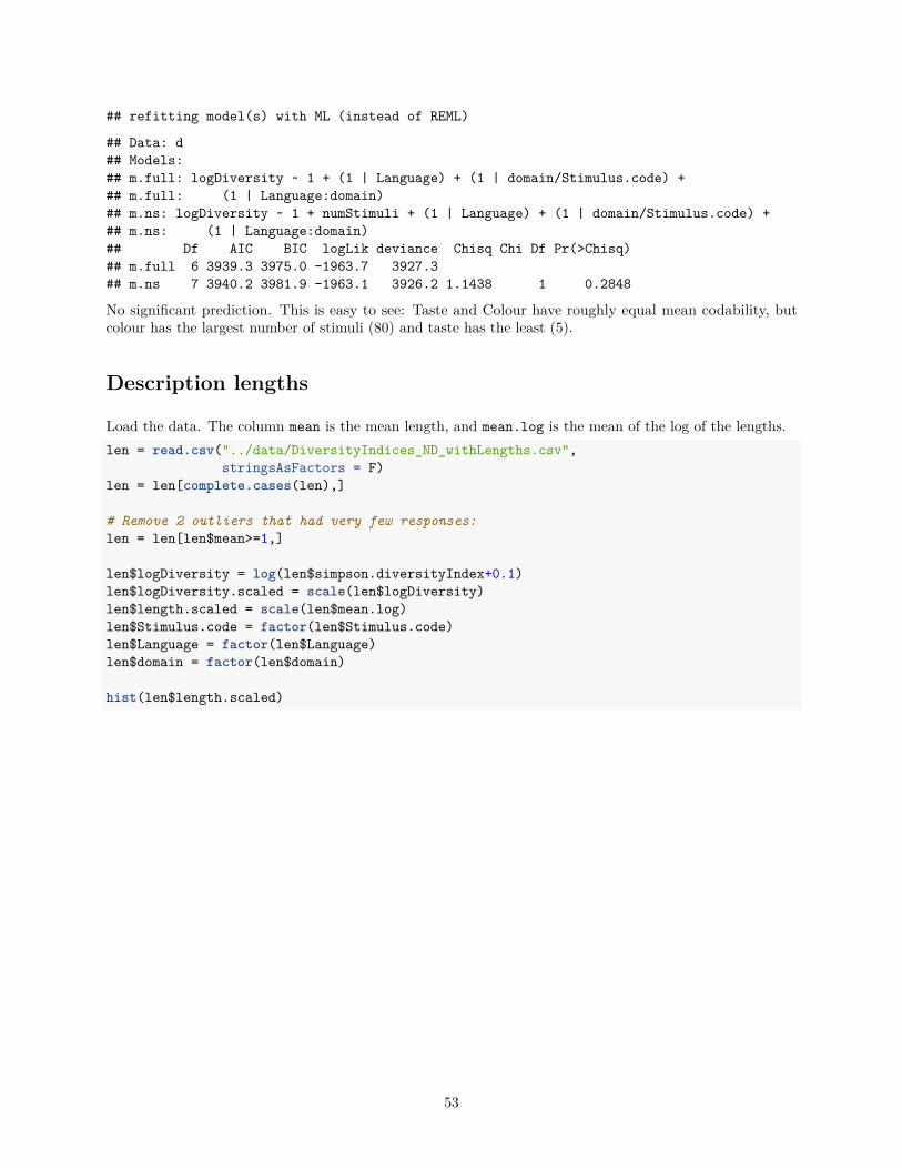
## refitting model(s) with ML (instead of REML)
## Data: d## Models:## m.full: logDiversity ~ 1 + (1 | Language) + (1 | domain/Stimulus.code) +## m.full: (1 | Language:domain)## m.ns: logDiversity ~ 1 + numStimuli + (1 | Language) + (1 | domain/Stimulus.code) +## m.ns: (1 | Language:domain)## Df AIC BIC logLik deviance Chisq Chi Df Pr(>Chisq)## m.full 6 3939.3 3975.0 -1963.7 3927.3## m.ns 7 3940.2 3981.9 -1963.1 3926.2 1.1438 1 0.2848
No significant prediction. This is easy to see: Taste and Colour have roughly equal mean codability, butcolour has the largest number of stimuli (80) and taste has the least (5).
Description lengths
Load the data. The column mean is the mean length, and mean.log is the mean of the log of the lengths.len = read.csv("../data/DiversityIndices_ND_withLengths.csv",
stringsAsFactors = F)len = len[complete.cases(len),]
# Remove 2 outliers that had very few responses:len = len[len$mean>=1,]
len$logDiversity = log(len$simpson.diversityIndex+0.1)len$logDiversity.scaled = scale(len$logDiversity)len$length.scaled = scale(len$mean.log)len$Stimulus.code = factor(len$Stimulus.code)len$Language = factor(len$Language)len$domain = factor(len$domain)
hist(len$length.scaled)
53

Histogram of len$length.scaled
len$length.scaled
Fre
quen
cy
−4 −2 0 2 4
020
040
060
080
0
Raw correlation:cor(len$mean.log, len$simpson.diversityIndex)
## [1] -0.1942662
Linear model with random intercepts and slopes by language, domain and the interaction between languageand domain:mLenl0 = lmer( logDiversity.scaled ~ 1 +
(1+length.scaled|Language) +(1+length.scaled|domain/Stimulus.code) +(1+length.scaled|Language:domain),
data=len)mLenl1 = update(mLenl0, ~.+length.scaled)mLenl2 = update(mLenl1, ~.+I(length.scaled^2))anova(mLenl0,mLenl1,mLenl2)
## refitting model(s) with ML (instead of REML)
## Data: len## Models:## mLenl0: logDiversity.scaled ~ 1 + (1 + length.scaled | Language) + (1 +## mLenl0: length.scaled | domain/Stimulus.code) + (1 + length.scaled |## mLenl0: Language:domain)## mLenl1: logDiversity.scaled ~ (1 + length.scaled | Language) + (1 + length.scaled |## mLenl1: domain/Stimulus.code) + (1 + length.scaled | Language:domain) +## mLenl1: length.scaled## mLenl2: logDiversity.scaled ~ (1 + length.scaled | Language) + (1 + length.scaled |## mLenl2: domain/Stimulus.code) + (1 + length.scaled | Language:domain) +## mLenl2: length.scaled + I(length.scaled^2)## Df AIC BIC logLik deviance Chisq Chi Df Pr(>Chisq)
54

## mLenl0 14 5049.5 5131.6 -2510.8 5021.5## mLenl1 15 5045.9 5133.9 -2508.0 5015.9 5.5888 1 0.01808 *## mLenl2 16 5046.7 5140.5 -2507.3 5014.7 1.2463 1 0.26426## ---## Signif. codes: 0 '***' 0.001 '**' 0.01 '*' 0.05 '.' 0.1 ' ' 1
There is a significant effect, but no quadratic effect. Since extremely short responses are unlikely to beinformative, we wondered if there were higher-level non-linear effects. We ran the same model as above, butas a generalised additive model (GAM):library(mgcv)library(itsadug)library(lmtest)mLen = bam(logDiversity.scaled ~
s(length.scaled) +s(Language,bs='re')+s(domain,bs='re')+s(Stimulus.code,bs='re')+s(Language,domain,bs='re'), # interaction
data = len)
Test for need for random slopes:mLen2 = update(mLen, ~.+s(Language,length.scaled,bs='re'))lrtest(mLen,mLen2)
## Likelihood ratio test#### Model 1: logDiversity.scaled ~ s(length.scaled) + s(Language, bs = "re") +## s(domain, bs = "re") + s(Stimulus.code, bs = "re") + s(Language,## domain, bs = "re")## Model 2: logDiversity.scaled ~ s(length.scaled) + s(Language, bs = "re") +## s(domain, bs = "re") + s(Stimulus.code, bs = "re") + s(Language,## domain, bs = "re") + s(Language, length.scaled, bs = "re")## #Df LogLik Df Chisq Pr(>Chisq)## 1 214.93 -2192.5## 2 232.94 -2103.9 18.008 177.13 < 2.2e-16 ***## ---## Signif. codes: 0 '***' 0.001 '**' 0.01 '*' 0.05 '.' 0.1 ' ' 1mLen3 = update(mLen2, ~.+s(domain,length.scaled,bs='re'))lrtest(mLen2,mLen3)
## Likelihood ratio test#### Model 1: logDiversity.scaled ~ s(length.scaled) + s(Language, bs = "re") +## s(domain, bs = "re") + s(Stimulus.code, bs = "re") + s(Language,## domain, bs = "re") + s(Language, length.scaled, bs = "re")## Model 2: logDiversity.scaled ~ s(length.scaled) + s(Language, bs = "re") +## s(domain, bs = "re") + s(Stimulus.code, bs = "re") + s(Language,## domain, bs = "re") + s(Language, length.scaled, bs = "re") +## s(domain, length.scaled, bs = "re")## #Df LogLik Df Chisq Pr(>Chisq)## 1 232.94 -2103.9## 2 235.20 -2097.8 2.2673 12.354 0.002077 **## ---## Signif. codes: 0 '***' 0.001 '**' 0.01 '*' 0.05 '.' 0.1 ' ' 1
55

mLen4 = update(mLen3, ~.+s(Stimulus.code,length.scaled,bs='re'))lrtest(mLen3,mLen4)
## Likelihood ratio test#### Model 1: logDiversity.scaled ~ s(length.scaled) + s(Language, bs = "re") +## s(domain, bs = "re") + s(Stimulus.code, bs = "re") + s(Language,## domain, bs = "re") + s(Language, length.scaled, bs = "re") +## s(domain, length.scaled, bs = "re")## Model 2: logDiversity.scaled ~ s(length.scaled) + s(Language, bs = "re") +## s(domain, bs = "re") + s(Stimulus.code, bs = "re") + s(Language,## domain, bs = "re") + s(Language, length.scaled, bs = "re") +## s(domain, length.scaled, bs = "re") + s(Stimulus.code, length.scaled,## bs = "re")## #Df LogLik Df Chisq Pr(>Chisq)## 1 235.2 -2097.8## 2 235.2 -2097.8 0.00010188 2e-04 < 2.2e-16 ***## ---## Signif. codes: 0 '***' 0.001 '**' 0.01 '*' 0.05 '.' 0.1 ' ' 1mLen5 = update(mLen4, ~.+s(Language,domain,length.scaled,bs='re'))lrtest(mLen4,mLen5)
## Likelihood ratio test#### Model 1: logDiversity.scaled ~ s(length.scaled) + s(Language, bs = "re") +## s(domain, bs = "re") + s(Stimulus.code, bs = "re") + s(Language,## domain, bs = "re") + s(Language, length.scaled, bs = "re") +## s(domain, length.scaled, bs = "re") + s(Stimulus.code, length.scaled,## bs = "re")## Model 2: logDiversity.scaled ~ s(length.scaled) + s(Language, bs = "re") +## s(domain, bs = "re") + s(Stimulus.code, bs = "re") + s(Language,## domain, bs = "re") + s(Language, length.scaled, bs = "re") +## s(domain, length.scaled, bs = "re") + s(Stimulus.code, length.scaled,## bs = "re") + s(Language, domain, length.scaled, bs = "re")## #Df LogLik Df Chisq Pr(>Chisq)## 1 235.20 -2097.8## 2 261.83 -2029.0 26.63 137.43 < 2.2e-16 ***## ---## Signif. codes: 0 '***' 0.001 '**' 0.01 '*' 0.05 '.' 0.1 ' ' 1
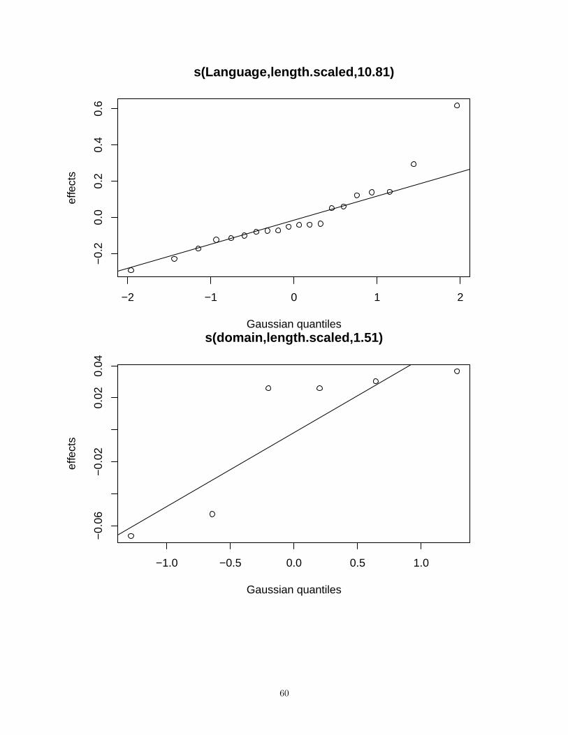
All random slopes improve the model. Final model:summary(mLen5)
#### Family: gaussian## Link function: identity#### Formula:## logDiversity.scaled ~ s(length.scaled) + s(Language, bs = "re") +## s(domain, bs = "re") + s(Stimulus.code, bs = "re") + s(Language,## domain, bs = "re") + s(Language, length.scaled, bs = "re") +## s(domain, length.scaled, bs = "re") + s(Stimulus.code, length.scaled,## bs = "re") + s(Language, domain, length.scaled, bs = "re")##
56

## Parametric coefficients:## Estimate Std. Error t value Pr(>|t|)## (Intercept) -0.1470 0.2136 -0.688 0.491#### Approximate significance of smooth terms:## edf Ref.df F p-value## s(length.scaled) 7.202e+00 8.23 5.177 1.29e-06 ***## s(Language) 1.351e+01 19.00 1565.987 3.54e-07 ***## s(domain) 4.489e+00 5.00 4818.072 2.96e-07 ***## s(Stimulus.code) 1.063e+02 131.00 8.931 6.37e-09 ***## s(Language,domain) 6.323e+01 113.00 279.468 3.16e-13 ***## s(Language,length.scaled) 1.081e+01 19.00 702.913 0.00188 **## s(domain,length.scaled) 1.507e+00 5.00 116.030 0.29047## s(Stimulus.code,length.scaled) 1.998e-05 131.00 0.000 0.99332## s(Language,domain,length.scaled) 5.003e+01 113.00 115.193 0.00236 **## ---## Signif. codes: 0 '***' 0.001 '**' 0.01 '*' 0.05 '.' 0.1 ' ' 1#### R-sq.(adj) = 0.691 Deviance explained = 72.2%## fREML = 2504 Scale est. = 0.30859 n = 2605
Note that there are significant random slopes for length by Language x domain and by Language, indicatingthat the stength of the length effect differes across cultures.
We can plot the model smooths.plot(mLen5)
−4 −2 0 2 4
−1.
5−
0.5
0.5
1.0
length.scaled
s(le
ngth
.sca
led,
7.2)
57

−2 −1 0 1 2
−0.
6−
0.2
0.0
0.2
0.4
s(Language,13.51)
Gaussian quantiles
effe
cts
−1.0 −0.5 0.0 0.5 1.0
−0.
6−
0.2
0.2
0.4
s(domain,4.49)
Gaussian quantiles
effe
cts
58

−2 −1 0 1 2
−0.
50.
00.
5
s(Stimulus.code,106.32)
Gaussian quantiles
effe
cts
−2 −1 0 1 2
−1.
0−
0.5
0.0
0.5
s(Language,domain,63.23)
Gaussian quantiles
effe
cts
59
−2 −1 0 1 2
−0.
20.
00.
20.
40.
6
s(Language,length.scaled,10.81)
Gaussian quantiles
effe
cts
−1.0 −0.5 0.0 0.5 1.0
−0.
06−
0.02
0.02
0.04
s(domain,length.scaled,1.51)
Gaussian quantiles
effe
cts
60
−2 −1 0 1 2
−4e
−08
0e+
004e
−08
s(Stimulus.code,length.scaled,0)
Gaussian quantiles
effe
cts
−2 −1 0 1 2
−0.
50.
00.
51.
0
s(Language,domain,length.scaled,50.03)
Gaussian quantiles
effe
cts
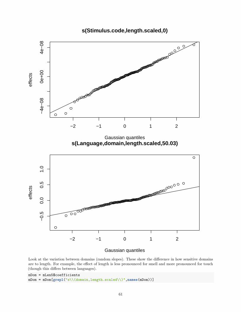
Look at the variation between domains (random slopes). These show the difference in how sensitive domainsare to length. For example, the effect of length is less pronounced for smell and more pronounced for touch(though this differs between languages).mDom = mLen5$coefficientsmDom = mDom[grepl("s\\(domain,length.scaled\\)",names(mDom))]
61

names(mDom) = as.character(levels(len$domain))t(t(sort(mDom)))
## [,1]## touch -0.06639260## taste -0.05270594## colour 0.02603199## sound 0.02606074## shape 0.03032637## smell 0.03667944
And between languages:mLang = mLen5$coefficientsmLang = mLang[grepl("s\\(Language,length.scaled\\)",names(mLang))]names(mLang) = as.character(levels(len$Language))t(t(sort(mLang)))
## [,1]## Yurakare -0.29214367## Dogul Dom -0.22843955## Tzeltal -0.17213762## BSL -0.12373691## Kilivila -0.11421187## Turkish -0.10026139## Kata Kolok -0.07953295## Semai -0.07343907## ASL -0.07220170## English -0.05093427## Farsi -0.04204591## Lao -0.03968849## Zapotec -0.03518524## Cantonese 0.05152590## Malay 0.05983917## Yucatec 0.12218071## Siwu 0.13851096## Mian 0.14155083## Yeli Dnye 0.29353532## Umpila 0.61681574
We can also use the itsadug library to plot the effect of length independent of the random effects. This alsoscales everything back into the original units, but cuts the length range to show 90% of the data (to hide thelong tail)convertLogDiversity = function(X){
# Convert the scaled diversity measure# back to the original unitsexp(X * attr(len$logDiversity.scaled,"scaled:scale") +
attr(len$logDiversity.scaled,"scaled:center"))-0.1}
px = plot_smooth(mLen5,view="length.scaled", rm.ranef = T, print.summary=F)
62

−4 −2 0 2 4
−2.
0−
1.0
0.0
0.5
1.0
length.scaled
logD
iver
sity
.sca
led
fitte
d va
lues
, exc
l. ra
ndom
px$fv$fit = convertLogDiversity(px$fv$fit)px$fv$ul = convertLogDiversity(px$fv$ul)px$fv$ll = convertLogDiversity(px$fv$ll)px$fv$length.scaled = exp(px$fv$length.scaled *
attr(len$length.scaled,"scaled:scale") +attr(len$length.scaled,"scaled:center"))-0.5
gLen = ggplot(px$fv, aes(x=length.scaled,y=fit)) +geom_ribbon(aes(ymin=ll,ymax=ul), alpha=0.3) +geom_line(size=1) +ylab("Codability") +xlab("Mean length of response") +coord_cartesian(xlim=c(0,quantile(len$mean, 0.90)))
gLen
63

0.0
0.2
0.4
0.6
0.8
0 10 20
Mean length of response
Cod
abili
ty
pdf("../results/graphs/Codability_by_Length.pdf",width = 4, height = 4)
gLendev.off()
## pdf## 2
64

S5: Test hierarchy of the senses
65

Test hierarchy
Load libraries
library(dplyr)library(Skillings.Mack)library(PMCMR)library(ggplot2)library(DyaDA)library(stringdist)
Note that the package DyaDA is still in development, and will need to be installed from github:#install.packages("devtools")#library(devtools)#install_github("DLEIVA/DyaDA")#library(DyaDA)
Load data
d = read.csv("../data/DiversityIndices_ND.csv", stringsAsFactors = F)
domain.order = c("colour","shape",'sound','touch','taste','smell')
d$domain = factor(d$domain, levels=domain.order, labels=c("Color","Shape","Sound","Touch","Taste","Smell"))
# Note spellingo f Yucatec / Yucatekd$Language = factor(d$Language,
levels =rev(c("English", "Farsi", "Turkish",
"Dogul Dom", "Siwu", "Cantonese", "Lao","Malay", "Semai", "Kilivila", "Mian","Yeli Dnye", "Umpila", "Tzeltal","Yucatec", "Zapotec", "Yurakare","ASL", "BSL", "Kata Kolok")),
labels =rev(c("English", "Farsi", "Turkish",
"Dogul Dom", "Siwu", "Cantonese", "Lao","Malay", "Semai", "Kilivila", "Mian","Yélî Dnye", "Umpila", "Tzeltal","Yucatec", "Zapotec", "Yurakare","ASL", "BSL", "Kata Kolok")))
labels= data.frame(Language=as.character(levels(d$Language)))labels$x = 1:nrow(labels)
Summarise diversity index by domain and language:d2 = d %>% group_by(Language,domain) %>%
summarise(m=mean(simpson.diversityIndex, na.rm=T),
66

upper=mean(simpson.diversityIndex)+sd(simpson.diversityIndex),lower=mean(simpson.diversityIndex)-sd(simpson.diversityIndex))
## Warning: package 'bindrcpp' was built under R version 3.3.2d2$rank = unlist(tapply(d2$m,d2$Language,rank))
67

Analyse hierarchy
There’s clearly no strict hierarchy. here is a table each domain’s rank number within each language. If thereas a strict hierarchy, then each domain would have a single rank number:table(d2$domain,d2$rank)
#### 1 2 3 4 5 6## Color 0 0 1 7 11 1## Shape 2 1 5 8 3 1## Sound 3 4 6 3 0 0## Touch 2 9 5 1 1 2## Taste 0 0 3 1 5 9## Smell 13 6 0 0 0 1
Calculate median codability.meanCodability = sapply(rev(as.character(unique(d2$Language))),function(l){
d2x = d2[as.character(d2$Language)==l,]mx = d2x$mnames(mx) = as.character(d2x$domain)mx[as.character(unique(d2$domain))]
})meanCodability = t(meanCodability)
68

Number of unique rank orders
Some languages have no data for some domains, so need to check whether each language is consistent withevery other language. The functions below calculate the number of unique compatible rank orders.matchCompatibleij = function(i,j,data){
# Take two row indices and check if the# ranks of the vectors of the rows in data# are in a compatible order.# Rows can include missing data.ix = data[i,]jx = data[j,]complete = !(is.na(ix)|is.na(jx))all(order(ix[complete])==order(jx[complete]))
}matchCompatible <- Vectorize(matchCompatibleij, vectorize.args=list("i","j"))
compatibleMatches = function(data){# Compare all individuals to all others,# checking if each is compatiblem = outer(1:nrow(data),1:nrow(data),matchCompatible,data=data)rownames(m) = rownames(data)colnames(m) = rownames(data)return(m)
}
matches = compatibleMatches(meanCodability)
Languages with unique rankings:names(which(rowSums(matches)==1))
## [1] "Dogul Dom" "Siwu" "Malay" "Kilivila" "Mian" "Yélî Dnye"## [7] "Umpila" "Tzeltal"
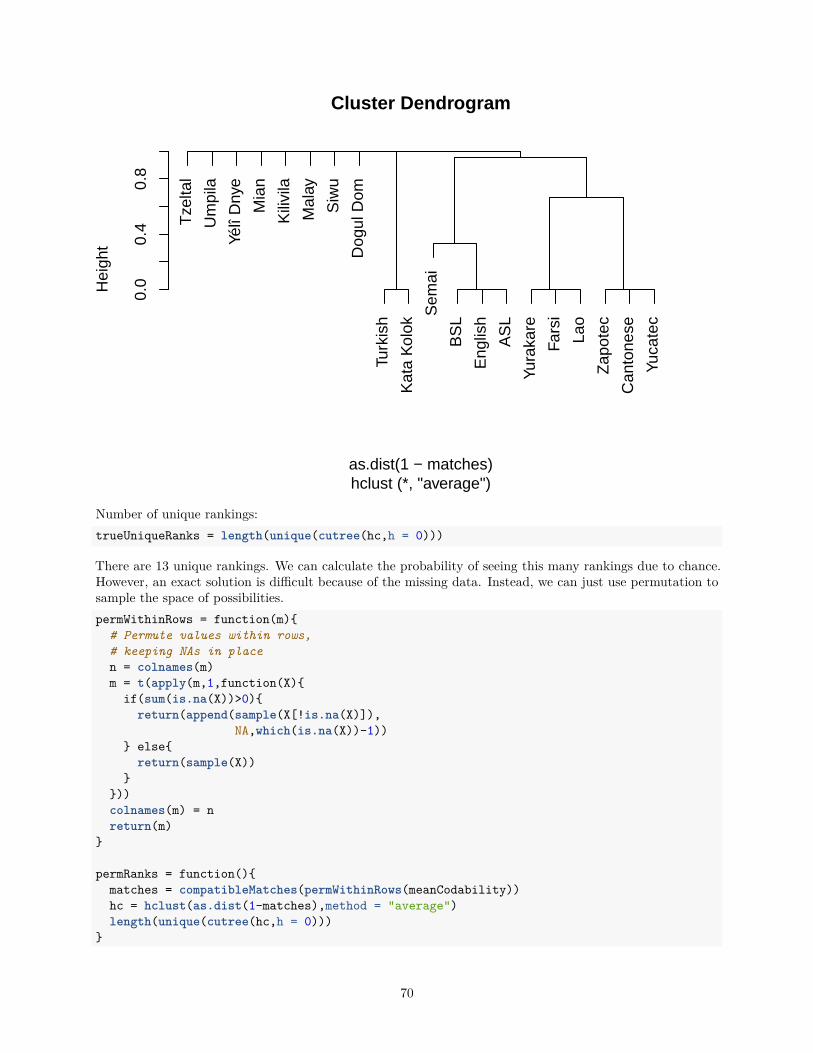
Use hierarchical clustering to identify unique rankings:hc = hclust(as.dist(1-matches),method = "average")plot(hc)
69
Tze
ltal
Um
pila
Yélî
Dny
e
Mia
n
Kili
vila
Mal
ay
Siw
u
Dog
ul D
om
Turk
ish
Kat
a K
olok
Sem
ai
BS
L
Eng
lish
AS
L
Yura
kare
Fars
i
Lao
Zap
otec
Can
tone
se
Yuca
tec
0.0
0.4
0.8
Cluster Dendrogram
hclust (*, "average")as.dist(1 − matches)
Hei
ght
Number of unique rankings:trueUniqueRanks = length(unique(cutree(hc,h = 0)))
There are 13 unique rankings. We can calculate the probability of seeing this many rankings due to chance.However, an exact solution is difficult because of the missing data. Instead, we can just use permutation tosample the space of possibilities.permWithinRows = function(m){
# Permute values within rows,# keeping NAs in placen = colnames(m)m = t(apply(m,1,function(X){
if(sum(is.na(X))>0){return(append(sample(X[!is.na(X)]),
NA,which(is.na(X))-1))} else{
return(sample(X))}
}))colnames(m) = nreturn(m)
}
permRanks = function(){matches = compatibleMatches(permWithinRows(meanCodability))hc = hclust(as.dist(1-matches),method = "average")length(unique(cutree(hc,h = 0)))
}
70

permUniqueRanks = replicate(10000,permRanks())
Compare true number of unique ranks to the permuted distribution:hist(permUniqueRanks,
xlim=range(c(permUniqueRanks,trueUniqueRanks)))abline(v=trueUniqueRanks,col=2)
Histogram of permUniqueRanks
permUniqueRanks
Fre
quen
cy
13 14 15 16 17 18 19 20
010
0020
0030
0040
00
p = sum(permUniqueRanks<=trueUniqueRanks)/length(permUniqueRanks)z = (trueUniqueRanks-mean(permUniqueRanks))/sd(permUniqueRanks)
The observed number of unique compatible ranks is less than would be expected by chance (z = -6.4586029,p < 0.001).
71

Aristotelian hierarchy
How compatible are the rank orderings with the Aristotelian hierarchy? This question is complicated by thefact that some languages do not have data for some domains, so each langauge needs to be assessed onlycomparing to those domains where data is available. The domains of colour and shape are also collapsedunder the category of “Sight”.
We’re using Spearman’s footrule to measure distance between rankings.aristotelian.order =c("Sight","Sight", "Sound", "Touch","Taste","Smell")
# Convert domains to senses (collapse colour and shape to sight)meanCodability.Senses = meanCodabilitycolnames(meanCodability.Senses) = c("Sight","Sight","Touch",'Taste',"Smell","Sound")
spearmanFootrule = function(v1,v2){# Version of Spearmans' footrule that can handle# Multiple tied rankssum(sapply(seq_along(v1), function(i) min(abs(i - (which(v2 == v1[i]))))))
}
spearmanFootruleFromAristotelanOrder = function(X){rk = names(sort(X,decreasing = T,na.last = NA))# filter aristotelian.order listao = aristotelian.order[aristotelian.order %in% rk]rk.rank = as.numeric(factor(rk,levels=unique(ao)))ao.rank = as.numeric(factor(ao,levels=unique(ao)))spearmanFootrule(rk.rank,ao.rank)
}
# Compare each language to the Aristotelian hierarchytrueNumEdits = apply(meanCodability.Senses,1,spearmanFootruleFromAristotelanOrder)t(t(trueNumEdits))
## [,1]## English 2## Farsi 9## Turkish 9## Dogul Dom 13## Siwu 13## Cantonese 7## Lao 9## Malay 4## Semai 2## Kilivila 7## Mian 4## Yélî Dnye 11## Umpila 15## Tzeltal 7## Yucatec 7## Zapotec 7## Yurakare 5## ASL 2
72

## BSL 2## Kata Kolok 7mean(trueNumEdits)
## [1] 7.1
Get expected Spearman’s footrule for each langage when permuting codability scores within languages(maintaining missing domain data).set.seed(1290)permutedNumEdits = replicate(10000,
apply(permWithinRows(meanCodability.Senses),1,spearmanFootruleFromAristotelanOrder))
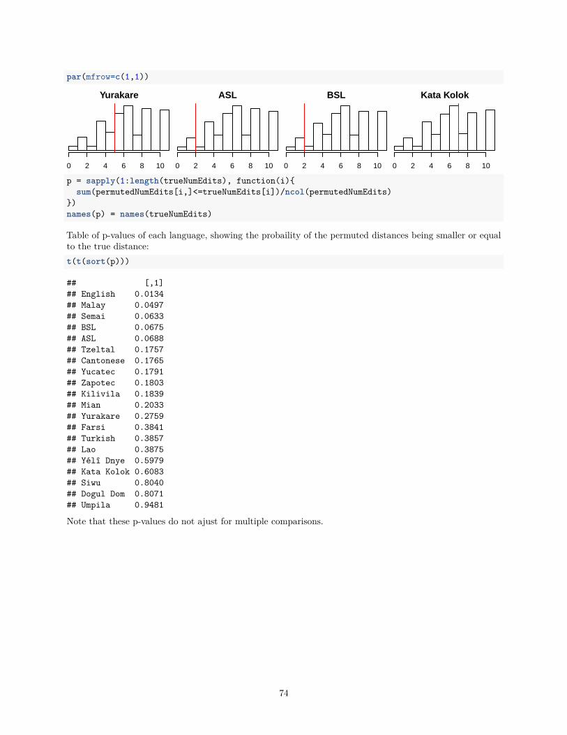
Analyse the difference:par(mfrow=c(4,4),mar=c(1,0,2,0))for(i in 1:length(trueNumEdits)){
hist(permutedNumEdits[i,],xlim=range(c(permutedNumEdits[i,],trueNumEdits[i])),main=names(trueNumEdits)[i],yaxt='n')
abline(v=trueNumEdits[i],col=2)}
English
permutedNumEdits[i, ]
0 5 10 15
Farsi
permutedNumEdits[i, ]
Fre
quen
cy
0 5 10 15
Turkish
permutedNumEdits[i, ]
Fre
quen
cy
0 5 10 15
Dogul Dom
permutedNumEdits[i, ]
Fre
quen
cy
0 5 10 15Siwu
permutedNumEdits[i, ]
0 5 10 15
Cantonese
permutedNumEdits[i, ]
Fre
quen
cy
0 5 10 15
Lao
permutedNumEdits[i, ]
Fre
quen
cy
0 5 10 15
Malay
permutedNumEdits[i, ]
Fre
quen
cy
0 5 10 15Semai
permutedNumEdits[i, ]
0 2 4 6 8 10
Kilivila
permutedNumEdits[i, ]
Fre
quen
cy
0 5 10 15
Mian
permutedNumEdits[i, ]
Fre
quen
cy
0 2 4 6 8 10
Yélî Dnye
permutedNumEdits[i, ]
Fre
quen
cy
0 5 10 15Umpila Tzeltal
Fre
quen
cy
Yucatec
Fre
quen
cy
Zapotec
Fre
quen
cy
73
par(mfrow=c(1,1))
Yurakare
permutedNumEdits[i, ]
0 2 4 6 8 10
ASL
permutedNumEdits[i, ]
Fre
quen
cy
0 2 4 6 8 10
BSL
permutedNumEdits[i, ]
Fre
quen
cy
0 2 4 6 8 10
Kata Kolok
permutedNumEdits[i, ]
Fre
quen
cy
0 2 4 6 8 10
p = sapply(1:length(trueNumEdits), function(i){sum(permutedNumEdits[i,]<=trueNumEdits[i])/ncol(permutedNumEdits)
})names(p) = names(trueNumEdits)
Table of p-values of each language, showing the probaility of the permuted distances being smaller or equalto the true distance:t(t(sort(p)))
## [,1]## English 0.0134## Malay 0.0497## Semai 0.0633## BSL 0.0675## ASL 0.0688## Tzeltal 0.1757## Cantonese 0.1765## Yucatec 0.1791## Zapotec 0.1803## Kilivila 0.1839## Mian 0.2033## Yurakare 0.2759## Farsi 0.3841## Turkish 0.3857## Lao 0.3875## Yélî Dnye 0.5979## Kata Kolok 0.6083## Siwu 0.8040## Dogul Dom 0.8071## Umpila 0.9481
Note that these p-values do not ajust for multiple comparisons.
74
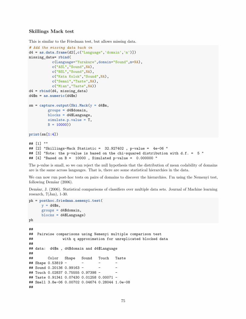
Skillings Mack test
This is similar to the Friedman test, but allows missing data.# Add the missing data back ind4 = as.data.frame(d2[,c("Language",'domain','m')])missing_data= rbind(
c(Language="Yurakare",domain="Sound",m=NA),c("ASL","Sound",NA),c("BSL","Sound",NA),c("Kata Kolok","Sound",NA),c("Semai","Taste",NA),c("Mian","Taste",NA))
d4 = rbind(d4, missing_data)d4$m = as.numeric(d4$m)
sm = capture.output(Ski.Mack(y = d4$m,groups = d4$domain,blocks = d4$Language,simulate.p.value = T,B = 10000))
print(sm[1:4])
## [1] ""## [2] "Skillings-Mack Statistic = 32.927402 , p-value = 4e-06 "## [3] "Note: the p-value is based on the chi-squared distribution with d.f. = 5 "## [4] "Based on B = 10000 , Simulated p-value = 0.000000 "
The p-value is small, so we can reject the null hypothesis that the distribution of mean codability of domainsare is the same across langauges. That is, there are some statistical hierarchies in the data.
We can now run post-hoc tests on pairs of domains to discover the hierarchies. I’m using the Nemenyi test,following Demšar (2006).
Demšar, J. (2006). Statistical comparisons of classifiers over multiple data sets. Journal of Machine learningresearch, 7(Jan), 1-30.ph = posthoc.friedman.nemenyi.test(
y = d4$m,groups = d4$domain,blocks = d4$Language)
ph
#### Pairwise comparisons using Nemenyi multiple comparison test## with q approximation for unreplicated blocked data#### data: d4$m , d4$domain and d4$Language#### Color Shape Sound Touch Taste## Shape 0.53819 - - - -## Sound 0.20136 0.99163 - - -## Touch 0.02837 0.75555 0.97398 - -## Taste 0.91341 0.07430 0.01258 0.00071 -## Smell 3.8e-06 0.00702 0.04674 0.28044 1.0e-08##
75

## P value adjustment method: none
Significant pairs:sig.threshold = 0.05
sig = which(ph$p.value<sig.threshold,arr.ind = T, useNames = F)sig[,1] = rownames(ph$p.value)[sig[,1]]sig[,2] = colnames(ph$p.value)[as.numeric(sig[,2])]
diff = sapply(1:nrow(sig), function(i){meanCodability[,sig[i,1]] -
meanCodability[,sig[i,2]]})
cnt = sapply(1:nrow(sig), function(i){max(sum(meanCodability[,sig[i,1]] >
meanCodability[,sig[i,2]],na.rm=T) ,sum(meanCodability[,sig[i,1]] <
meanCodability[,sig[i,2]],na.rm=T))})cnt.poss = apply(meanCodability,2,function(X){sum(!is.na(X))})
colnames(diff) = paste(sig[,1],"-",sig[,2])
ggplot(as.data.frame.table(diff),aes(x=Var2,y=Freq)) +
geom_hline(yintercept = 0) +geom_boxplot() +ylab("Difference in Simpson's diversity index") +xlab("Domains") +coord_flip()
76

Touch − Color
Smell − Color
Smell − Shape
Taste − Sound
Smell − Sound
Taste − Touch
Smell − Taste
−0.5 0.0 0.5Difference in Simpson's diversity index
Dom
ains
Summarise the patterns alongside the statistics:mdiff = colMeans(diff,na.rm = T)direction = c(">","<")[1+(mdiff>0)]ruleLables = sapply(1:nrow(sig), function(i){
if(mdiff[i]>0){return(paste(sig[i,2],"<",sig[i,1]))
} else{return(paste(sig[i,1],"<",sig[i,2]))
}})ruleP = ph$p.value[ph$p.value<sig.threshold & !is.na(ph$p.value)]ruleP = signif(ruleP,2)ruleP[ruleP<0.001] = "< 0.001"paste(ruleLables,"(p =",ruleP,",",
cnt,"/",cnt.poss,"languages)")
## [1] "Touch < Color (p = 0.028 , 17 / 20 languages)"## [2] "Smell < Color (p = < 0.001 , 19 / 20 languages)"## [3] "Smell < Shape (p = 0.007 , 18 / 20 languages)"## [4] "Sound < Taste (p = 0.013 , 13 / 18 languages)"## [5] "Smell < Sound (p = 0.047 , 12 / 20 languages)"## [6] "Touch < Taste (p = < 0.001 , 16 / 16 languages)"## [7] "Smell < Taste (p = < 0.001 , 17 / 20 languages)"
77

Linearity test
We use algorithms from ethology for converting a matrix of wins and losses in dyadic interactions into aconsistent linear hierarchy. That is, we treat domains as “individuals” and see in how many languages adomain “dominantes” (more codable than) another.
Build a dominance matrix:domain.labels = c("Color","Shape","Sound","Touch","Taste","Smell")
m = apply(expand.grid(domain.labels,domain.labels),1, function(X){#gt = d2[d2$domain==X[1],]$m > d2[d2$domain==X[2],]$mgt = meanCodability[,X[1]]>meanCodability[,X[2]]sum(gt,na.rm=T)
})m = matrix(m,nrow=length(domain.labels), ncol=length(domain.labels))rownames(m) = domain.labelscolnames(m) = domain.labelsm
## Color Shape Sound Touch Taste Smell## Color 0 16 16 17 4 19## Shape 4 0 12 14 4 18## Sound 0 4 0 8 1 12## Touch 3 6 8 0 2 17## Taste 14 14 13 16 0 17## Smell 1 2 4 3 1 0
In the table above, e.g. Colour is more codable than Smell in 19 languages.
Run the linearity test:set.seed(3298)linear.hierarchy.test(m)
#### Linearity test: Landau's h## ==========================###### Number of individuals: 6 ( 15 dyads)## Total number of interactions: 270#### Descriptive table of dyadic relationships:## Frequency Percentage## Unknown 0 0.00000## Tied 1 6.66667## One-way 1 6.66667## Two-way 14 93.33333## Significant 11 73.33333#### Landau's h index: 0.971429## E(h): 0.428571## Var(h): 0.083333## Improved Landau's h: 0.971429## Number of randomizations: 9999## P-value (right): 0.0229
78
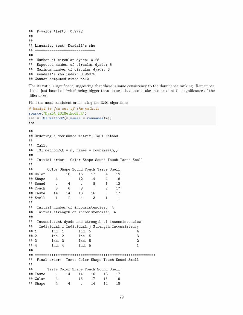
## P-value (left): 0.9772###### Linearity test: Kendall's rho## =============================#### Number of circular dyads: 0.25## Expected number of circular dyads: 5## Maximum number of circular dyads: 8## Kendall's rho index: 0.96875## Cannot computed since n<10.
The statistic is significant, suggesting that there is some consistency to the dominance ranking. Remember,this is just based on ‘wins’ being bigger than ‘losses’, it doesn’t take into account the significance of thedifferences.
Find the most consistent order using the I&SI algorithm:# Needed to fix one of the methodssource("DyaDA_ISIMethod2.R")isi = ISI.method2(m,names = rownames(m))isi
#### Ordering a dominance matrix: I&SI Method#### Call:## ISI.method2(X = m, names = rownames(m))#### Initial order: Color Shape Sound Touch Taste Smell#### Color Shape Sound Touch Taste Smell## Color . 16 16 17 4 19## Shape 4 . 12 14 4 18## Sound . 4 . 8 1 12## Touch 3 6 8 . 2 17## Taste 14 14 13 16 . 17## Smell 1 2 4 3 1 .#### Initial number of inconsistencies: 4## Initial strength of incosistencies: 4#### Inconsistent dyads and strength of inconsistencies:## Individual.i Individual.j Strength.Inconsistency## 1 Ind. 1 Ind. 5 4## 2 Ind. 2 Ind. 5 3## 3 Ind. 3 Ind. 5 2## 4 Ind. 4 Ind. 5 1#### **********************************************************## Final order: Taste Color Shape Touch Sound Smell#### Taste Color Shape Touch Sound Smell## Taste . 14 14 16 13 17## Color 4 . 16 17 16 19## Shape 4 4 . 14 12 18
79

## Touch 2 3 6 . 8 17## Sound 1 . 4 8 . 12## Smell 1 1 2 3 4 .#### Final number of inconsistencies: 0## Final strength of inconsistencies: 0#### Inconsistent dyads and strength of inconsistencies:## [1] NA
The linear order most consistent with the domain ranking within languages is (according to the I&SIalgorithm):best.order= rownames(isi$dataFinal)paste(best.order,collapse =">")
## [1] "Taste>Color>Shape>Touch>Sound>Smell"
Again, you can’t interpret this as “Touch is significantly more codable than sound”, it’s just an order that isconsistent with each domain being more codable in more languages than the last.actual.orders = apply(meanCodability,1,function(X){
x = rev(colnames(meanCodability)[order(X)])all(x == best.order[best.order %in% x])
})sum(actual.orders)
## [1] 0which(actual.orders)
## named integer(0)
There are no languages that are compatible with this order, so it’s a poor approximation.
80

S6: Explaining Codability
81

Explaining codability
ContentsIntroduction 82
Load libraries 85
Load data 85
General properties 87
Specific domains 98
Colour 98Colour Results . . . . . . . . . . . . . . . . . . . . . . . . . . . . . . . . . . . . . . . . . . . . . . . 98
Shape 104Shape Results . . . . . . . . . . . . . . . . . . . . . . . . . . . . . . . . . . . . . . . . . . . . . . . . 104Specific hypotheses about shape . . . . . . . . . . . . . . . . . . . . . . . . . . . . . . . . . . . . . 109
Sound 111Sound Results . . . . . . . . . . . . . . . . . . . . . . . . . . . . . . . . . . . . . . . . . . . . . . . . 111
Touch 114Touch Results . . . . . . . . . . . . . . . . . . . . . . . . . . . . . . . . . . . . . . . . . . . . . . . . 114
Taste 115Taste Results . . . . . . . . . . . . . . . . . . . . . . . . . . . . . . . . . . . . . . . . . . . . . . . . 115Specific taste hypotheses . . . . . . . . . . . . . . . . . . . . . . . . . . . . . . . . . . . . . . . . . . 116
Smell 118Smell Results . . . . . . . . . . . . . . . . . . . . . . . . . . . . . . . . . . . . . . . . . . . . . . . . 118
Extra Graphs 124
Introduction
This set of analyses tries to explain the codability scores according to non-linguistic factors. A list of a-priorihypotheses about external factors that could influence agreement in each domain was compiled. The analysisof agreement across domains used a linear mixed effects model with random effects for domains nested withinlanguages and for stimuli nested within domains. Predictor variables were added to the model as fixed effectsand remained if they significantly improved the model according to log likelihood comparison.
The factors that were predicted to explain general levels of codability within a population are:
• Number of speakers of the language (from Ethnologue or field linguist’s estimate)• Formal schooling (low, medium, high)• Subsistance type (hunter-gatherer, horticultural, stable agriculture, industrial, post-industrial)• Environment type (closed, open, both)• Environment subtype (urban, jungle, fields, rocky plateau, forest, forest & sea)• Settlement type (nucleated, dispersed)• Society has a market (yes, no)
82

• Society supports specialists (yes, no)
The Environment subtype variable was too varied to provide meaningful explanation in such a small sample,so is left out of this analysis.
For domains where predictor variables were highly co-linear, a two-step approach was taken. A randomforests regression with random intercepts for languages was used to predict variation in agreement accordingto all a-priori predictor variables. Variable importance measures were used to identify key variables. Theeffect of these variables was tested with a full mixed effects model with random intercepts for language andstimulus.
The hypotheses for each domain were as follows:
Colour
• Presence of paints• Number of paints (none, few, many)• Presence of dyes• Number of dyes (none, few, many)• Ritual use of colour (yes, no)• Professional colour (yes, no)• Coloured (yes, no)• Weaving patterns (yes, no)
Shape
• formal schooling (low, medium, high)• pottery (yes, no)• patterned pottery (yes, no)• containers (yes, no)• number of abstract shape categories (none, one, many)• professional builders (yes, no)• society makes boats (yes, no)• boat specialists (yes, no)• craft specialists (yes, no)• spinning thread (yes, no)• weaving (yes, no)• weaving specialists (yes, no)• weave patterns (yes, no)• what weave patterns (none < simple < angular < complex)• leatherware (yes, no)• decorated.leatherware (yes, no)
In addition, it is predicted that communities living in round houses will have lower codability for angularshapes than those living in angular (square or rectangular) houses.
Sound
• musical instrument (yes, no)• specialist musician (yes, no)• training music (yes, no)• children music (yes, no)• animal sounds (yes, no)
83

Touch
• pulverise spices (yes, no)• fine surfaces on houses (yes, no)• professional textures (yes, no)
Taste
• pulverise.spices (yes, no)• spices herbs (yes, no)• Number of additives (0-5)• sweet additive (for sweet stimulus, yes, no)• salt additive (for salty stimulus, yes, no)• bitter additive (for bitter stimulus, yes, no)• sour additive (for sour stimulus, yes, no)• umami additive (for umami stimulus, yes, no)• fragrant food (yes, no)
In addition, having particular additives is predicted to increase the codability for the particular taste stimuli.
Smell
• pulverise spices (yes, no)• spices herbs (yes, no)• fragrant food (yes, no)• Subsistance type (particularly hunter-gratherers)• latitude (proxy for humidity)
Colinearity
These pairs of variables that are co-linear in our sample, meaning that it is redundant to add them both:
• “market”, “spices/herbs”• “pottery coloured”, “spinning specialists”• “pottery coloured”, “leatherware”• “spinning specialists”, “leatherware”• “decorated leatherware”, “what leatherware patterns?”• “pulverise spices”, “sweet additive”• “pulverise spices”, “sour additive”• “sweet additive”, “sour additive”
84

Load libraries
library(party)library(rpart.plot)library(XLConnect)library(reshape2)library(ggplot2)library(usdm)library(REEMtree)library(lme4)library(sjPlot)library(gridExtra)
Load data
s = read.csv("../data/DiversityIndices_ND.csv")
ethnography = read.csv("../data/ethnography/LoP_ethnography_processed.csv")
v.with.variation = apply(ethnography,2,function(X){length(unique(X))>1})
ethnography = ethnography[,v.with.variation]
ethnography$paints.cat =factor(ethnography$paints.cat,
levels=c("none",'few','many'),ordered = TRUE)
ethnography$dyes.cat =factor(ethnography$dyes.cat,
levels=c("none",'few','many'),ordered = TRUE)
ethnography$ritual.colour.cat =factor(ethnography$dyes.cat,
levels=c("none",'few','many'),ordered = TRUE)
ethnography$environment =factor(ethnography$environment,
levels = c("closed",'both','open'))
ethnography$subsistance =factor(ethnography$subsistance,
levels = c("hunter-gatherer","horticultural",'stable agriculture','industrial',"post-industrial"), ordered = T)
ethnography$formal.schooling =factor(ethnography$formal.schooling,
levels = c("low",'medium','high'), ordered = T)
85

ethnography$num.additives.scaled = scale(ethnography$num.additives)
ethnography$what.weave.patterns2 =factor(ethnography$what.weave.patterns2,
levels=c("no",'simple','angular','complex'),ordered = T)
ethnography$shape2 = "many"ethnography$shape2[ethnography$shape =="no"] = "none"ethnography$shape2[ethnography$shape %in% c("oblong",'cylinderical','round')] = "one"ethnography$shape2 = factor(ethnography$shape2,
levels=c("none",'one','many'),ordered = T)
# Add ethnography data to diversity scoress = cbind(s,
ethnography[match(s$Language,ethnography$Language),!names(ethnography) %in%
c("Language","Language.orig")])
s$pop.logcenter = scale(log(s$pop))
# Cut population into 3 categories# (may not be used)s$pop.cat = cut(s$pop.logcenter,
quantile(s$pop.logcenter,probs=seq(0,1,length.out=4)),
include.lowest = T,labels = c("Low","Medium","High"))
# Transform the diversity index to log scale# (note that this does not actually change the results much)s$simpson.diversityIndex.log = log(0.1+s$simpson.diversityIndex)# scale and centers$simpson.diversityIndex.log = scale(s$simpson.diversityIndex.log)
Set random seed:set.seed(9999)
86

General properties
Use a mixed effects model to test whether the overall codability is affected by general properties of thecommunities. We start with a null model and add variables if their inclusion significantly improves the fit ofthe model.
We are quite conservative here, and add random effects for domains within languages and also for stimuliwithin domains.m0 = lmer(simpson.diversityIndex.log~
1 +(1 | Language/domain) +(1|domain/Stimulus.code),data = s)
mPop = update(m0, ~.+pop.logcenter)anova(m0,mPop)
## refitting model(s) with ML (instead of REML)
## Data: s## Models:## m0: simpson.diversityIndex.log ~ 1 + (1 | Language/domain) + (1 |## m0: domain/Stimulus.code)## mPop: simpson.diversityIndex.log ~ (1 | Language/domain) + (1 | domain/Stimulus.code) +## mPop: pop.logcenter## Df AIC BIC logLik deviance Chisq Chi Df Pr(>Chisq)## m0 6 5909.4 5945.1 -2948.7 5897.4## mPop 7 5896.1 5937.7 -2941.0 5882.1 15.353 1 8.918e-05 ***## ---## Signif. codes: 0 '***' 0.001 '**' 0.01 '*' 0.05 '.' 0.1 ' ' 1mEnv = update(mPop, ~.+environment)anova(mPop,mEnv)
## refitting model(s) with ML (instead of REML)
## Data: s## Models:## mPop: simpson.diversityIndex.log ~ (1 | Language/domain) + (1 | domain/Stimulus.code) +## mPop: pop.logcenter## mEnv: simpson.diversityIndex.log ~ (1 | Language/domain) + (1 | domain/Stimulus.code) +## mEnv: pop.logcenter + environment## Df AIC BIC logLik deviance Chisq Chi Df Pr(>Chisq)## mPop 7 5896.1 5937.7 -2941.0 5882.1## mEnv 9 5897.2 5950.8 -2939.6 5879.2 2.8746 2 0.2376mEnvD = update(mPop, ~.+environment.details)anova(mPop,mEnvD)
## refitting model(s) with ML (instead of REML)
## Data: s## Models:## mPop: simpson.diversityIndex.log ~ (1 | Language/domain) + (1 | domain/Stimulus.code) +## mPop: pop.logcenter## mEnvD: simpson.diversityIndex.log ~ (1 | Language/domain) + (1 | domain/Stimulus.code) +## mEnvD: pop.logcenter + environment.details## Df AIC BIC logLik deviance Chisq Chi Df Pr(>Chisq)## mPop 7 5896.1 5937.7 -2941 5882.1
87

## mEnvD 12 5900.0 5971.5 -2938 5876.0 6.0605 5 0.3004mSett = update(mPop, ~.+settlement)anova(mPop, mSett)
## refitting model(s) with ML (instead of REML)
## Data: s## Models:## mPop: simpson.diversityIndex.log ~ (1 | Language/domain) + (1 | domain/Stimulus.code) +## mPop: pop.logcenter## mSett: simpson.diversityIndex.log ~ (1 | Language/domain) + (1 | domain/Stimulus.code) +## mSett: pop.logcenter + settlement## Df AIC BIC logLik deviance Chisq Chi Df Pr(>Chisq)## mPop 7 5896.1 5937.7 -2941 5882.1## mSett 8 5898.0 5945.7 -2941 5882.0 0.0121 1 0.9125mMark = update(mPop, ~.+market)anova(mPop,mMark)
## refitting model(s) with ML (instead of REML)
## Data: s## Models:## mPop: simpson.diversityIndex.log ~ (1 | Language/domain) + (1 | domain/Stimulus.code) +## mPop: pop.logcenter## mMark: simpson.diversityIndex.log ~ (1 | Language/domain) + (1 | domain/Stimulus.code) +## mMark: pop.logcenter + market## Df AIC BIC logLik deviance Chisq Chi Df Pr(>Chisq)## mPop 7 5896.1 5937.7 -2941.0 5882.1## mMark 8 5896.8 5944.5 -2940.4 5880.8 1.2432 1 0.2649mSpec = update(mPop, ~.+specialists)anova(mPop,mSpec)
## refitting model(s) with ML (instead of REML)
## Data: s## Models:## mPop: simpson.diversityIndex.log ~ (1 | Language/domain) + (1 | domain/Stimulus.code) +## mPop: pop.logcenter## mSpec: simpson.diversityIndex.log ~ (1 | Language/domain) + (1 | domain/Stimulus.code) +## mSpec: pop.logcenter + specialists## Df AIC BIC logLik deviance Chisq Chi Df Pr(>Chisq)## mPop 7 5896.1 5937.7 -2941.0 5882.1## mSpec 8 5897.9 5945.5 -2940.9 5881.9 0.1514 1 0.6972mSubs = update(mPop, ~.+subsistance)anova(mPop,mSubs)
## refitting model(s) with ML (instead of REML)
## Data: s## Models:## mPop: simpson.diversityIndex.log ~ (1 | Language/domain) + (1 | domain/Stimulus.code) +## mPop: pop.logcenter## mSubs: simpson.diversityIndex.log ~ (1 | Language/domain) + (1 | domain/Stimulus.code) +## mSubs: pop.logcenter + subsistance## Df AIC BIC logLik deviance Chisq Chi Df Pr(>Chisq)
88

## mPop 7 5896.1 5937.7 -2941.0 5882.1## mSubs 11 5898.9 5964.4 -2938.4 5876.9 5.1745 4 0.2699mScho = update(mPop, ~.+formal.schooling)anova(mPop,mScho)
## refitting model(s) with ML (instead of REML)
## Data: s## Models:## mPop: simpson.diversityIndex.log ~ (1 | Language/domain) + (1 | domain/Stimulus.code) +## mPop: pop.logcenter## mScho: simpson.diversityIndex.log ~ (1 | Language/domain) + (1 | domain/Stimulus.code) +## mScho: pop.logcenter + formal.schooling## Df AIC BIC logLik deviance Chisq Chi Df Pr(>Chisq)## mPop 7 5896.1 5937.7 -2941.0 5882.1## mScho 9 5894.3 5947.9 -2938.2 5876.3 5.7206 2 0.05725 .## ---## Signif. codes: 0 '***' 0.001 '**' 0.01 '*' 0.05 '.' 0.1 ' ' 1
The only significant variable is population size. We can also test whether the relationship survives allowingfor random slopes by domain (random slopes by language don’t make sense because population doesn’t varyby language).m0.popSlope = lmer(simpson.diversityIndex.log~
1 +(1 | Language/domain) +(1 +pop.logcenter|domain/Stimulus.code),
data = s)mPop2 = update(m0.popSlope, ~.+pop.logcenter)anova(m0.popSlope,mPop2)
## refitting model(s) with ML (instead of REML)
## Data: s## Models:## m0.popSlope: simpson.diversityIndex.log ~ 1 + (1 | Language/domain) + (1 +## m0.popSlope: pop.logcenter | domain/Stimulus.code)## mPop2: simpson.diversityIndex.log ~ (1 | Language/domain) + (1 + pop.logcenter |## mPop2: domain/Stimulus.code) + pop.logcenter## Df AIC BIC logLik deviance Chisq Chi Df Pr(>Chisq)## m0.popSlope 10 5751.5 5811.0 -2865.7 5731.5## mPop2 11 5748.7 5814.2 -2863.3 5726.7 4.7884 1 0.02865 *## ---## Signif. codes: 0 '***' 0.001 '**' 0.01 '*' 0.05 '.' 0.1 ' ' 1summary(mPop2)
## Linear mixed model fit by REML ['lmerMod']## Formula:## simpson.diversityIndex.log ~ (1 | Language/domain) + (1 + pop.logcenter |## domain/Stimulus.code) + pop.logcenter## Data: s#### REML criterion at convergence: 5731.5#### Scaled residuals:## Min 1Q Median 3Q Max
89

## -2.9443 -0.6193 0.0218 0.6113 3.6973#### Random effects:## Groups Name Variance Std.Dev. Corr## Stimulus.code:domain (Intercept) 0.129513 0.35988## pop.logcenter 0.040504 0.20126 -0.01## domain:Language (Intercept) 0.220798 0.46989## Language (Intercept) 0.006338 0.07961## domain (Intercept) 0.233937 0.48367## pop.logcenter 0.039240 0.19809 0.80## Residual 0.331665 0.57590## Number of obs: 2850, groups:## Stimulus.code:domain, 147; domain:Language, 114; Language, 20; domain, 6#### Fixed effects:## Estimate Std. Error t value## (Intercept) -0.21071 0.20785 -1.014## pop.logcenter 0.24036 0.09763 2.462#### Correlation of Fixed Effects:## (Intr)## pop.logcntr 0.633
Statistical summary: There was a significant main effect of population size predicting general agreement ( loglikelihood difference = 2.4 , df = 1 , Chi Squared = 4.79 , p = 0.029 ).
90

Plot the random effects:sjp.lmer(mPop2, 're', sort.est = "(Intercept)")
## Plotting random effects...## Plotting random effects...
−0.86−0.75−0.70−0.67−0.66−0.65−0.64−0.63−0.60−0.58−0.56−0.43−0.40−0.40−0.40−0.39−0.39−0.38−0.38−0.37−0.36−0.36−0.33−0.33−0.32−0.32−0.32−0.30−0.29−0.28−0.26−0.24−0.24−0.24−0.24−0.23−0.23−0.21−0.20−0.20−0.19−0.18−0.18−0.16−0.16−0.16−0.16−0.15−0.15−0.15−0.14−0.13−0.10−0.10−0.09−0.09−0.08−0.08−0.07−0.07−0.06−0.06−0.06−0.04−0.04−0.04−0.04−0.03−0.03−0.020.010.020.020.020.030.030.030.040.050.060.070.080.080.080.090.090.090.090.090.100.100.100.100.110.120.130.140.150.150.160.160.160.170.170.180.200.200.200.210.210.230.230.230.240.250.260.270.270.270.280.280.290.300.300.310.320.320.320.320.350.350.360.390.410.420.470.470.510.550.570.580.580.660.700.740.770.94
−0.11−0.03−0.10−0.13−0.12−0.01−0.13−0.090.05−0.13−0.290.130.100.15−0.030.260.200.050.08−0.30 0.230.120.260.060.26−0.050.160.06−0.080.02−0.03−0.280.080.01−0.06−0.35−0.040.050.170.24−0.050.01−0.23 0.29−0.200.03−0.04−0.31−0.220.18−0.100.32−0.120.280.070.32−0.04−0.05−0.38−0.050.16−0.120.11−0.04−0.39−0.11−0.160.010.310.24−0.02−0.160.00−0.090.04−0.020.28−0.180.15−0.38−0.030.15−0.070.16−0.010.26−0.020.04−0.090.070.220.01−0.010.280.050.100.05−0.070.090.12−0.07−0.16−0.150.03−0.080.010.000.230.16−0.41 0.150.17−0.050.13−0.02−0.040.150.100.13−0.37−0.07−0.05−0.000.160.030.09−0.08−0.08−0.19−0.00−0.11−0.43 0.140.03−0.45 0.130.070.050.030.010.020.080.080.06−0.06−0.28−0.10(Intercept) pop.logcenter
−1.0 −0.5 0.0 0.5 1.0 −1.0 −0.5 0.0 0.5 1.0sound.sound.tempo.4b:soundcolour.5R 2/8:colourcolour.5Y 4/6:coloursound.sound.tempo.7a:soundsound.sound.tempo.7b:soundcolour.10R 8/6:colourcolour.10RP 2/8:colourcolour.5Y 6/10:colourcolour.5R 8/6:coloursound.sound.tempo.4a:soundshape.flower:shapecolour.10YR 4/8:colourshape.cone:shapecolour.10RP 8/6:colourcolour.5YR 8/8:colourcolour.5P 6/8:colourshape.cylinder:shapeshape.3 cones:shapesmell.smoke:smellcolour.10YR 6/12:colourcolour.5RP 2/8:colourcolour.10P 2/6:colourcolour.5YR 4/8:colourcolour.10P 6/10:colourcolour.10PB 6/10:colourtaste.glutamate (umami):tastecolour.10PB 4/12:colourcolour.5YR 2/4:colourtouch.curved ridges (wide spacing):touchtouch.beads:touchtouch.straight ridges (small spacing):touchshape.elipsoid:shapecolour.10Y 6/10:colourcolour.10BG 8/4:colourcolour.10BG 4/6:colourcolour.5RP 4/12:coloursmell.lemon:smellsmell.gasoline:smellcolour.5P 2/8:colourcolour.10R 2/6:colourtouch.cork:touchcolour.10BG 6/8:colourcolour.5B 2/6:colourshape.2 triangles:shapecolour.5P 8/4:colourcolour.10P 4/12:coloursmell.paint thinner:smellcolour.5GY 2/2:colourcolour.5BG 8/4:colourcolour.5GY 8/10:colourshape.rectangle 3D:shapecolour.5P 4/12:colourshape.sphere:shapecolour.10P 8/6:colourcolour.10Y 4/6:colourcolour.5RP 8/6:coloursound.sound.loud−up.1a:soundsmell.turpentine:smellcolour.10R 4/12:colourshape.cube:shapecolour.10PB 2/10:colourshape.2 spheres:shapecolour.5B 8/4:coloursmell.onion:smellcolour.5R 6/12:colourcolour.10BG 2/6:colourcolour.10YR 2/2:coloursmell.chocolate:smellcolour.5PB 8/6:colourshape.rectangle:shapetouch.felt:touchshape.2 cubes:shapesound.sound.pitch−up.2a:soundcolour.10GY 2/4:colourcolour.5YR 6/14:coloursmell.soap:smellcolour.10B 8/6:coloursmell.pineapple:smellsound.sound.loud−down.6a:soundcolour.10PB 8/4:coloursound.sound.pitch−down.8a:soundcolour.5B 4/10:colourtaste.citric acide monohydrate (sour):tastecolour.5B 6/10:colourcolour.10R 6/14:colourshape.3 squares:shapesound.sound.loud−down.3b:soundsmell.rose:smellshape.elipse:shapetaste.quinine hydrochloride (bitter):tastecolour.5PB 6/10:colourcolour.5PB 2/8:coloursound.sound.pitch−down.5a:soundshape.triangle:shapesmell.banana:smellsound.sound.loud−up.10b:soundsound.sound.pitch−down.8b:soundtouch.feather:touchtouch.fur (synthetic):touchcolour.5RP 6/12:colourcolour.10G 2/6:colourcolour.5BG 6/10:colourshape.3 elipses:shapesound.sound.loud−up.10a:soundcolour.5BG 2/6:colourcolour.10B 2/6:coloursound.sound.loud−down.6b:soundcolour.10B 6/10:coloursound.sound.loud−up.1b:soundcolour.5Y 2/2:colourshape.2 circles:shapeshape.square:shapecolour.5G 2/6:colourtouch.jagged (fabric):touchtaste.sodium chloride (salt):tastecolour.10Y 8/12:coloursound.sound.pitch−up.2b:soundsound.sound.pitch−up.9b:soundcolour.5GY 4/8:colourcolour.10RP 6/12:colourtouch.plastic (sheet):touchsound.sound.pitch−up.9a:soundcolour.10YR 8/14:colourcolour.10B 4/10:colourcolour.10G 8/6:colourshape.circle:shapesound.sound.pitch−down.5b:soundcolour.5BG 4/8:colourtouch.rubber (yoga mat):touchcolour.5G 8/6:colourtaste.sucrose (sweet):tastecolour.10Y 2/2:colourcolour.5PB 4/12:coloursound.sound.loud−down.3a:soundcolour.10RP 4/14:coloursmell.cinnamon:smellcolour.10GY 8/8:colourcolour.5GY 6/10:colourcolour.10G 6/10:colourcolour.5G 6/10:colourcolour.10GY 4/8:colourcolour.5Y 8/14:colourcolour.5G 4/10:colourcolour.10GY 6/12:colourcolour.10G 4/10:colourcolour.5R 4/14:colourshape.star:shape
BLUP
Gro
up le
vels
## Plotting random effects...
91

−1.00−0.88−0.85−0.78−0.75−0.74−0.67−0.66−0.63−0.62−0.62−0.59−0.55−0.52−0.51−0.48−0.47−0.43−0.42−0.38−0.38−0.34−0.32−0.32−0.31−0.31−0.31−0.30−0.29−0.27−0.26−0.25−0.24−0.23−0.22−0.21−0.20−0.19−0.18−0.17−0.16−0.15−0.11−0.10−0.10−0.09−0.09−0.08−0.07−0.07−0.06−0.06−0.05−0.05−0.05−0.05−0.03−0.02−0.02−0.000.050.050.060.060.070.070.070.070.070.100.130.130.130.140.140.160.170.230.240.260.270.270.280.290.310.310.310.320.320.340.370.370.370.380.410.430.430.430.430.450.490.510.520.580.580.590.640.640.660.700.880.920.971.09(Intercept)
−1.0 −0.5 0.0 0.5 1.0 1.5shape:Dogul Domsound:Farsitaste:BSLtaste:Englishcolour:Kata Kolokshape:Tzeltaltaste:ASLcolour:Umpilatouch:Kata Koloksound:Siwutouch:ASLsound:Kilivilataste:Malayshape:Umpilacolour:Kilivilatouch:BSLshape:Yeli Dnyesmell:Zapoteccolour:Yeli Dnyecolour:Laosmell:Yurakaresmell:Cantonesesmell:ASLsound:Malaysmell:Miantouch:Turkishsmell:BSLtouch:Umpilacolour:Turkishsmell:Kilivilatouch:Cantonesetouch:Englishsound:Yeli Dnyesmell:Tzeltaltouch:Farsishape:Laosmell:Semaicolour:Englishsmell:Englishtouch:Yucateccolour:Siwutaste:Umpilacolour:Farsitouch:Yurakaresound:Miansmell:Malaytouch:Kilivilashape:Englishsmell:Kata Koloksmell:Yeli Dnyecolour:Semaishape:Farsishape:Siwusound:Laosound:Umpilatouch:Semaishape:Yurakareshape:Semaismell:Yucateccolour:Malaytaste:Kata Koloksound:Dogul Domshape:BSLsound:Englishshape:Kata Koloktaste:Siwusmell:Dogul Domsmell:Farsishape:Kilivilataste:Yeli Dnyecolour:Yurakaretouch:Malaycolour:Cantonesetaste:Dogul Domtaste:Turkishtaste:Kilivilashape:Turkishsound:Semaismell:Turkishtouch:Zapotectouch:Tzeltalshape:Zapotectaste:Yurakareshape:Mianshape:Malaysmell:Siwusound:Cantonesetaste:Cantonesetouch:Miansound:Zapoteccolour:Tzeltalcolour:Dogul Domtouch:Laotouch:Yeli Dnyecolour:Yucatectaste:Yucatectaste:Farsishape:Yucatecshape:Cantonesetaste:Zapotecsound:Turkishshape:ASLsound:Tzeltalcolour:ASLcolour:Zapotectaste:Tzeltalsound:Yucatectaste:Laocolour:BSLcolour:Miansmell:Laotouch:Siwusmell:Umpilatouch:Dogul Dom
BLUP
Gro
up le
vels
## Plotting random effects...
92

−0.04−0.04−0.03
−0.03−0.02−0.02−0.02−0.02−0.01
−0.00−0.00
0.010.010.020.020.020.03
0.040.04
0.05
(Intercept)
−0.2 −0.1 0.0 0.1 0.2
English
Kata Kolok
Kilivila
BSL
Farsi
Umpila
Yeli Dnye
ASL
Malay
Yurakare
Semai
Turkish
Siwu
Cantonese
Dogul Dom
Tzeltal
Mian
Lao
Zapotec
Yucatec
BLUP
Gro
up le
vels
−0.71
−0.24
−0.14
0.13
0.47
0.49
−0.24
−0.17
−0.03
0.17
0.17
0.10
(Intercept) pop.logcenter
−1.0 −0.5 0.0 0.5 −1.0 −0.5 0.0 0.5
smell
touch
sound
shape
colour
taste
BLUP
Gro
up le
vels
Plot the model effects for population size (extra code is to scale everything back into real numbers):
93

popxcod = data.frame(population=tapply(s$pop.logcenter,s$Language, mean),mean.codability =
tapply(s$simpson.diversityIndex.log,s$Language,mean))
popxcod$population = exp((popxcod$population*attr(s$pop.logcenter,'scaled:scale')) +
attr(s$pop.logcenter,'scaled:center'))
popxcod$mean.codability = exp(((popxcod$mean.codability*attr(s$simpson.diversityIndex.log,'scaled:scale')) +
attr(s$simpson.diversityIndex.log,'scaled:center')))-0.1
plotsX = sjp.lmer(mPop2, "eff", show.ci = T,show.scatter = T,prnt.plot=F,facet.grid=F)
## Warning: package 'bindrcpp' was built under R version 3.3.2plotsX$plot.list[[1]]$labels$title = ""
plotsX$plot.list[[1]]$data$x =exp((plotsX$plot.list[[1]]$data$x*attr(s$pop.logcenter,'scaled:scale')) +
attr(s$pop.logcenter,'scaled:center'))
plotsX$plot.list[[1]]$data$y =exp(((plotsX$plot.list[[1]]$data$y*attr(s$simpson.diversityIndex.log,'scaled:scale')) +
attr(s$simpson.diversityIndex.log,'scaled:center')))-0.1
plotsX$plot.list[[1]]$data$lower =exp(((plotsX$plot.list[[1]]$data$lower*attr(s$simpson.diversityIndex.log,'scaled:scale')) +
attr(s$simpson.diversityIndex.log,'scaled:center')))-0.1
plotsX$plot.list[[1]]$data$upper =exp(((plotsX$plot.list[[1]]$data$upper*attr(s$simpson.diversityIndex.log,'scaled:scale')) +
attr(s$simpson.diversityIndex.log,'scaled:center')))-0.1
gx.pop = plotsX$plot.list[[1]] +scale_x_log10() +xlab("Population size") +ylab("Codability") +ggtitle("Overall codability") +geom_point(data=popxcod, aes(population,mean.codability))
gx.pop
94

0.2
0.4
0.6
1e+03 1e+05 1e+07 1e+09
Population size
Cod
abili
tyOverall codability
Plots for subsistance, formal schooling.ggplot(s,
aes(subsistance,simpson.diversityIndex)) +geom_boxplot() +xlab("Subsistance type") +ylab("Codability")
95

0.00
0.25
0.50
0.75
1.00
hunter−gatherer horticultural stable agriculture industrial post−industrial
Subsistance type
Cod
abili
ty
gg.formalschooling =ggplot(s,
aes(formal.schooling,simpson.diversityIndex)) +geom_boxplot() +xlab("Formal schooling") +ylab("Codability")
gg.formalschooling
96

0.00
0.25
0.50
0.75
1.00
low medium high
Formal schooling
Cod
abili
ty
Correlation between population size and subsistance:kruskal.test(ethnography$pop, ethnography$subsistance)
#### Kruskal-Wallis rank sum test#### data: ethnography$pop and ethnography$subsistance## Kruskal-Wallis chi-squared = 12.004, df = 4, p-value = 0.01732
97

Specific domains
There are many more variables to consider for the individual domains. Many are highly correlated, and thereare many missing combinations in the data. This makes a regression approach difficult. Instead, we can usea binary decision tree to find clusters in the data based on salient properties. The package REEMtree alsoallows an additional random effect for Language (crossed random effects for stimulus type are not permitted).So we use random forests to identify key variables (or exclude unimportant variables), then mixed effectsmodelling to determine significance of main effects.
Note that we’re using a categorical version of the population variable that splits the data into“small”,“medium”,‘large’. This is because the raw population variable is a continuous variable that can beused by a decision tree to split the languages into many arbitrary categories, giving it an unfair advantageover the other variables and making it difficult to interpret the plot.
Colour
Calculate the optimal decision tree, given variables related to colour:s.colour = s[s$domain=='colour',]rt = REEMtree(simpson.diversityIndex~
formal.schooling +paints.cat+dyes.cat+ritual.colour.cat+professional.colour+pottery.coloured+weave.patterns,
random = ~1|Language,data = s.colour,MaxIterations=100000)
Colour Results
Proportion of variance explained:# R squaredcor(predict.REEMtree(rt,s.colour,id=s.colour$Language,
EstimateRandomEffects = T),s.colour$simpson.diversityIndex)^2
## [1] 0.3132261
Plot the tree and calculate variable importance:rpart.plot(tree(rt), type=4,extra=100, branch.lty=1, box.palette="RdYlGn", main="Colour")
98
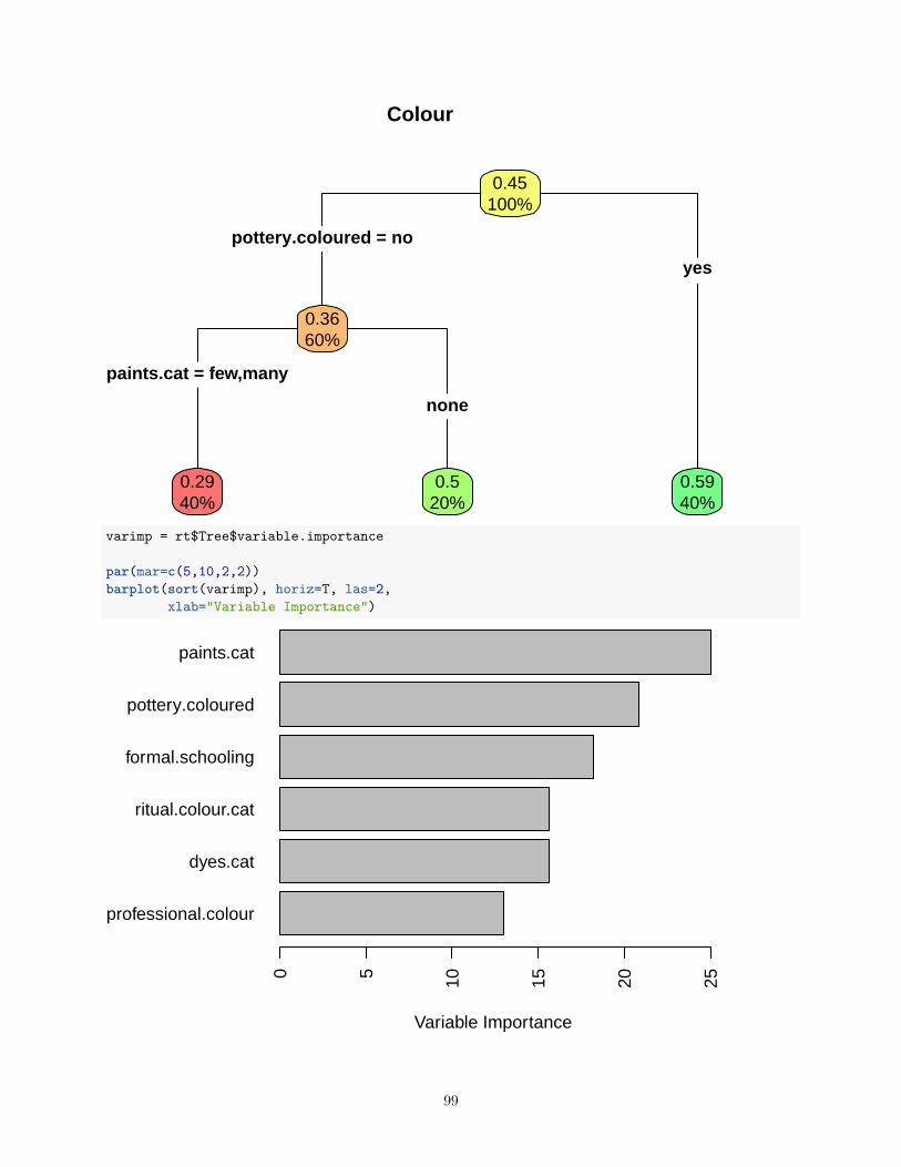
Colour
pottery.coloured = no
paints.cat = few,many
yes
none
0.45100%
0.3660%
0.2940%
0.520%
0.5940%
varimp = rt$Tree$variable.importance
par(mar=c(5,10,2,2))barplot(sort(varimp), horiz=T, las=2,
xlab="Variable Importance")
professional.colour
dyes.cat
ritual.colour.cat
formal.schooling
pottery.coloured
paints.cat
Variable Importance
0 5 10 15 20 25
99

par(mar=c(5, 4, 4, 2) + 0.1)
Plot the relationships:ggplot(s.colour,
aes(pottery.coloured,simpson.diversityIndex)) +geom_boxplot() +xlab("Coloured pottery") +ylab("Codability")
0.00
0.25
0.50
0.75
1.00
no yes
Coloured pottery
Cod
abili
ty
ggplot(s.colour,aes(paints.cat,simpson.diversityIndex)) +
geom_boxplot() +xlab("Number of paints")
100

0.00
0.25
0.50
0.75
1.00
none few many
Number of paints
sim
pson
.div
ersi
tyIn
dex
ggplot(s.colour,aes(formal.schooling,simpson.diversityIndex)) +
geom_boxplot() +xlab("Formal Schooling")
101

0.00
0.25
0.50
0.75
1.00
low medium high
Formal Schooling
sim
pson
.div
ersi
tyIn
dex
Test the most important variables with a mixed effects model:mc.all = lmer(simpson.diversityIndex.log ~
1 +paints.cat +pottery.coloured +formal.schooling +
(1 | Language) +(1 | Stimulus.code),
data = s.colour)
mc.noPaints = lmer(simpson.diversityIndex.log ~1 +
pottery.coloured +formal.schooling +
(1 | Language) +(1 | Stimulus.code),
data = s.colour)
mc.noSchool = lmer(simpson.diversityIndex.log ~1 +
pottery.coloured +paints.cat +
(1 | Language) +(1 | Stimulus.code),
data = s.colour)
102

mc.noPott = lmer(simpson.diversityIndex.log ~1 +
paints.cat +formal.schooling +
(1 | Language) +(1 | Stimulus.code),
data = s.colour)
anova(mc.all, mc.noPaints)
## refitting model(s) with ML (instead of REML)
## Data: s.colour## Models:## mc.noPaints: simpson.diversityIndex.log ~ 1 + pottery.coloured + formal.schooling +## mc.noPaints: (1 | Language) + (1 | Stimulus.code)## mc.all: simpson.diversityIndex.log ~ 1 + paints.cat + pottery.coloured +## mc.all: formal.schooling + (1 | Language) + (1 | Stimulus.code)## Df AIC BIC logLik deviance Chisq Chi Df Pr(>Chisq)## mc.noPaints 7 3396.1 3433.8 -1691.1 3382.1## mc.all 9 3390.2 3438.6 -1686.1 3372.2 9.925 2 0.006996 **## ---## Signif. codes: 0 '***' 0.001 '**' 0.01 '*' 0.05 '.' 0.1 ' ' 1anova(mc.all, mc.noSchool)
## refitting model(s) with ML (instead of REML)
## Data: s.colour## Models:## mc.noSchool: simpson.diversityIndex.log ~ 1 + pottery.coloured + paints.cat +## mc.noSchool: (1 | Language) + (1 | Stimulus.code)## mc.all: simpson.diversityIndex.log ~ 1 + paints.cat + pottery.coloured +## mc.all: formal.schooling + (1 | Language) + (1 | Stimulus.code)## Df AIC BIC logLik deviance Chisq Chi Df Pr(>Chisq)## mc.noSchool 7 3386.7 3424.3 -1686.3 3372.7## mc.all 9 3390.2 3438.6 -1686.1 3372.2 0.5037 2 0.7774anova(mc.all, mc.noPott)
## refitting model(s) with ML (instead of REML)
## Data: s.colour## Models:## mc.noPott: simpson.diversityIndex.log ~ 1 + paints.cat + formal.schooling +## mc.noPott: (1 | Language) + (1 | Stimulus.code)## mc.all: simpson.diversityIndex.log ~ 1 + paints.cat + pottery.coloured +## mc.all: formal.schooling + (1 | Language) + (1 | Stimulus.code)## Df AIC BIC logLik deviance Chisq Chi Df Pr(>Chisq)## mc.noPott 8 3388.4 3431.4 -1686.2 3372.4## mc.all 9 3390.2 3438.6 -1686.1 3372.2 0.1791 1 0.6721
There is only a contribution of number of paints beyond population size, but this goes in the opposite directionof the predicted one: societies with few paints have fewer categories than societies with none or many. Therewas a significant main effect of number of paints ( log likelihood difference = 5 , df = 2 , Chi Squared = 9.92, p = 0.007 ).
103

Shape
Calculate the optimal decision tree, given variables related to shape:s.shape = s[s$domain=='shape',]
rt.shape = REEMtree(simpson.diversityIndex~formal.schooling +pottery +pottery.patterned +containers +shape2 +professional.builders +make.boats+boat.specialists+craft.specialists+spinning.thread+weaving+weaving.specialists+weave.patterns+what.weave.patterns2+leatherware+decorated.leatherware,
random = ~1|Language,data = s.shape,MaxIterations=100000)
Shape Results
Proportion of variance explained:# R squaredcor(predict.REEMtree(rt.shape,s.shape,id=s.shape$Language, EstimateRandomEffects = T),
s.shape$simpson.diversityIndex)^2
## [1] 0.4100091
Plot the tree and calculate variable importance:rpart.plot(tree(rt.shape), type=4,extra=100, branch.lty=1, box.palette="RdYlGn", main="Shape")
104

Shape
pottery.patterned = no
yes
0.32100%
0.260%
0.5140%
varimp = rt.shape$Tree$variable.importance
par(mar=c(5,10,2,2))barplot(sort(varimp), horiz=T, las=2,
xlab="Variable Importance")
boat.specialists
decorated.leatherware
leatherware
pottery
formal.schooling
pottery.patterned
Variable Importance
0 2 4 6 8
par(mar=c(5, 4, 4, 2) + 0.1)
Both pottery.patterned and formal.schooling have high importance. The two variables are highlyco-linear (there are no societies with ‘high’ formal schooling without patterned pottery):
105

table(s$formal.schooling, s$pottery.patterned)
#### no yes## low 1131 147## medium 583 0## high 0 989
So we can look at both:gx.shape = ggplot(s.shape, aes(pottery.patterned, simpson.diversityIndex))+
geom_boxplot() +xlab("Patterned pottery") +ylab("Codability")+ggtitle("Codability of Shape")
gx.shape
0.00
0.25
0.50
0.75
1.00
no yes
Patterned pottery
Cod
abili
ty
Codability of Shape
gx.shape2 = ggplot(s.shape, aes(formal.schooling, simpson.diversityIndex))+geom_boxplot() +xlab("Formal Schooling") +ylab("Codability") +ggtitle("Codability of Shape")
gx.shape2
106

0.00
0.25
0.50
0.75
1.00
low medium high
Formal Schooling
Cod
abili
tyCodability of Shape
And use a mixed effects model to test the contribuion of each:m.both = lmer(simpson.diversityIndex.log ~
pottery.patterned +formal.schooling +(1 | Language) +(1 | Stimulus.code),
data = s.shape)
m.noSchool = lmer(simpson.diversityIndex.log ~pottery.patterned +(1 | Language) +(1 | Stimulus.code),
data = s.shape)
m.noPPottery = lmer(simpson.diversityIndex.log ~formal.schooling +(1 | Language) +(1 | Stimulus.code),
data = s.shape)
anova(m.both,m.noSchool)
## refitting model(s) with ML (instead of REML)
## Data: s.shape## Models:## m.noSchool: simpson.diversityIndex.log ~ pottery.patterned + (1 | Language) +
107
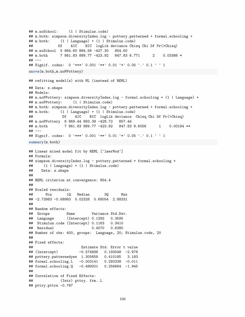
## m.noSchool: (1 | Stimulus.code)## m.both: simpson.diversityIndex.log ~ pottery.patterned + formal.schooling +## m.both: (1 | Language) + (1 | Stimulus.code)## Df AIC BIC logLik deviance Chisq Chi Df Pr(>Chisq)## m.noSchool 5 864.60 884.56 -427.30 854.60## m.both 7 861.83 889.77 -423.92 847.83 6.771 2 0.03386 *## ---## Signif. codes: 0 '***' 0.001 '**' 0.01 '*' 0.05 '.' 0.1 ' ' 1anova(m.both,m.noPPottery)
## refitting model(s) with ML (instead of REML)
## Data: s.shape## Models:## m.noPPottery: simpson.diversityIndex.log ~ formal.schooling + (1 | Language) +## m.noPPottery: (1 | Stimulus.code)## m.both: simpson.diversityIndex.log ~ pottery.patterned + formal.schooling +## m.both: (1 | Language) + (1 | Stimulus.code)## Df AIC BIC logLik deviance Chisq Chi Df Pr(>Chisq)## m.noPPottery 6 869.44 893.39 -428.72 857.44## m.both 7 861.83 889.77 -423.92 847.83 9.6056 1 0.00194 **## ---## Signif. codes: 0 '***' 0.001 '**' 0.01 '*' 0.05 '.' 0.1 ' ' 1summary(m.both)
## Linear mixed model fit by REML ['lmerMod']## Formula:## simpson.diversityIndex.log ~ pottery.patterned + formal.schooling +## (1 | Language) + (1 | Stimulus.code)## Data: s.shape#### REML criterion at convergence: 854.4#### Scaled residuals:## Min 1Q Median 3Q Max## -2.73983 -0.68983 0.02328 0.68054 2.88331#### Random effects:## Groups Name Variance Std.Dev.## Language (Intercept) 0.1292 0.3595## Stimulus.code (Intercept) 0.1163 0.3410## Residual 0.4070 0.6380## Number of obs: 400, groups: Language, 20; Stimulus.code, 20#### Fixed effects:## Estimate Std. Error t value## (Intercept) -0.574896 0.193048 -2.978## pottery.patternedyes 1.305659 0.410185 3.183## formal.schooling.L -0.003141 0.292338 -0.011## formal.schooling.Q -0.499201 0.256664 -1.945#### Correlation of Fixed Effects:## (Intr) pttry. frm..L## pttry.pttrn -0.787
108

## frml.schl.L 0.714 -0.882## frml.schl.Q 0.469 -0.725 0.658# R squared:cor(s.shape$simpson.diversityIndex.log,predict(m.both))^2
## [,1]## [1,] 0.6122963# Mtapply(s.shape$simpson.diversityIndex,s.shape$formal.schooling,mean)
## low medium high## 0.1946866 0.2803914 0.5109820
There was a significant main effect of schooling ( log likelihood difference = 3.4 , df = 2 , Chi Squared = 6.77, p = 0.034 ).
There was a significant main effect of patterned pottery ( log likelihood difference = 4.8 , df = 1 , Chi Squared= 9.61 , p = 0.0019 ).
Specific hypotheses about shape
Natural objects have (mostly) organic rounded shapes. Living in square/rectangular houses should givemore names for angular shaped objects. We test whether living in rounded houses predicts codability forangular shapes. Note that there is only one community which lives in round houses (Umpila). Umpila areHunter-gatherers, who are not necessarily low-codability across the board (they have very high codability forsmell).s.shape$angularShapes = s.shape$Stimulus.code %in%
c("shape.2 cubes","shape.3 squares",'shape.cube','shape.square','shape.rectangle','shape.rectangle 3D')
# Null modelm0 = lmer(simpson.diversityIndex.log ~
1 +(1 | Language) +(1 +I(houses=="round")| Stimulus.code),
data = s.shape[s.shape$angularShapes,])# Add fixed effectm1 = lmer(simpson.diversityIndex.log ~
1 +I(houses=="round") +(1 | Language) +(1 +I(houses=="round")| Stimulus.code),
data = s.shape[s.shape$angularShapes,])anova(m0,m1)
## refitting model(s) with ML (instead of REML)
## Data: s.shape[s.shape$angularShapes, ]## Models:## m0: simpson.diversityIndex.log ~ 1 + (1 | Language) + (1 + I(houses ==## m0: "round") | Stimulus.code)
109

## m1: simpson.diversityIndex.log ~ 1 + I(houses == "round") + (1 |## m1: Language) + (1 + I(houses == "round") | Stimulus.code)## Df AIC BIC logLik deviance Chisq Chi Df Pr(>Chisq)## m0 6 256.70 273.43 -122.35 244.70## m1 7 254.77 274.29 -120.39 240.77 3.9308 1 0.04741 *## ---## Signif. codes: 0 '***' 0.001 '**' 0.01 '*' 0.05 '.' 0.1 ' ' 1summary(m1)
## Linear mixed model fit by REML ['lmerMod']## Formula: simpson.diversityIndex.log ~ 1 + I(houses == "round") + (1 |## Language) + (1 + I(houses == "round") | Stimulus.code)## Data: s.shape[s.shape$angularShapes, ]#### REML criterion at convergence: 240.8#### Scaled residuals:## Min 1Q Median 3Q Max## -2.87221 -0.58415 -0.00682 0.59798 2.95397#### Random effects:## Groups Name Variance Std.Dev. Corr## Language (Intercept) 0.645532 0.80345## Stimulus.code (Intercept) 0.009365 0.09677## I(houses == "round")TRUE 0.017855 0.13362 -1.00## Residual 0.276179 0.52553## Number of obs: 120, groups: Language, 20; Stimulus.code, 6#### Fixed effects:## Estimate Std. Error t value## (Intercept) -0.01047 0.19483 -0.054## I(houses == "round")TRUE -1.69196 0.85495 -1.979#### Correlation of Fixed Effects:## (Intr)## I(=="")TRUE -0.231
Very weak significant effect for communities with rounded houses to have less agreement on angular shapesthan those living in angular houses. Mean codability for angular houses = 0.35153; mean codability for roundhouses = 0.0121212gx.shape.house = ggplot(s.shape[s.shape$angularShapes,],
aes(houses!="round",simpson.diversityIndex)) +xlab("House shape") +scale_x_discrete(labels=c("Round","Angular")) +ylab("Codability") +geom_boxplot()
110

Sound
Calculate the optimal decision tree, given variables related to shape:s.sound = s[s$domain=='sound',]
rt.sound = REEMtree(simpson.diversityIndex~musical.instrument +specialist.musician+training.music+children.music+animal.sounds,
random = ~1|Language,data = s.sound,MaxIterations=100000,tree.control = rpart.control(maxdepth = 1))
Sound Results
Proportion of variance explained:# R squaredcor(predict.REEMtree(rt.sound,s.sound,id=s.sound$Language, EstimateRandomEffects = T),
s.sound$simpson.diversityIndex)^2
## [1] 0.4052415
Plot the tree and calculate variable importance:rpart.plot(tree(rt.sound), type=4,extra=100,
branch.lty=1, box.palette="RdYlGn", main="Sound")
Sound
specialist.musician = no
animal.sounds = yes
children.music = yes
yes
no
no
0.24100%
0.1119%
0.2781%
0.238%
0.112%
0.2525%
0.3344%
111

This suggests that the training of musicians and having specialist musicians is important. Training ofmusicians depends on having specialist musicians, so we concentrate on the latter.gx.sound = ggplot(s.sound, aes(specialist.musician, simpson.diversityIndex))+
geom_boxplot() +xlab("Specialist musicians") +ylab("Codability") +ggtitle("Codability of sounds")
gx.sound
0.00
0.25
0.50
0.75
1.00
no yes
Specialist musicians
Cod
abili
ty
Codability of sounds
Test with mixed effects modelling:mSd.null = lmer(simpson.diversityIndex.log ~
1 +(1 | Language) +(1 | Stimulus.code),
data = s.sound)
mSd.music = lmer(simpson.diversityIndex.log ~1 +
specialist.musician +(1 | Language) +(1 | Stimulus.code),
data = s.sound)
anova(mSd.null, mSd.music)
## refitting model(s) with ML (instead of REML)
112

## Data: s.sound## Models:## mSd.null: simpson.diversityIndex.log ~ 1 + (1 | Language) + (1 | Stimulus.code)## mSd.music: simpson.diversityIndex.log ~ 1 + specialist.musician + (1 | Language) +## mSd.music: (1 | Stimulus.code)## Df AIC BIC logLik deviance Chisq Chi Df Pr(>Chisq)## mSd.null 4 540.57 555.64 -266.29 532.57## mSd.music 5 538.47 557.31 -264.24 528.47 4.1008 1 0.04286 *## ---## Signif. codes: 0 '***' 0.001 '**' 0.01 '*' 0.05 '.' 0.1 ' ' 1#Mtapply(s.sound$simpson.diversityIndex,s.sound$specialist.musician,mean)
## no yes## 0.1101010 0.2709464
113

Touch
Calculate the optimal decision tree, given variables related to shape:s.touch = s[s$domain=='touch',]
rt.touch = REEMtree(simpson.diversityIndex~pulverise.spices +fine.surfaces.on.houses +professional.textures,
random = ~1|Language,data = s.touch,MaxIterations=100000)
Touch Results
Proportion of variance explained:# R squaredcor(predict.REEMtree(rt.touch,s.touch,id=s.touch$Language, EstimateRandomEffects = T),
s.touch$simpson.diversityIndex)^2
## [1] 0.4448271
Plot the tree and calculate variable importance:rpart.plot(tree(rt.touch), type=4,extra=100, branch.lty=1, box.palette="RdYlGn", main="Touch")
Touch
0.22100%
#varimp = rt.touch$Tree$variable.importance
#par(mar=c(5,10,2,2))#barplot(sort(varimp), horiz=T, las=2,# xlab="Variable Importance")#par(mar=c(5, 4, 4, 2) + 0.1)
There are no significant partitions for touch.
114

Taste
Calculate the optimal decision tree, given variables related to taste:
(some variables are co-linear, so we take out sweet.addivit ve and sour.additive)s.taste = s[s$domain=='taste',]
rt.taste = REEMtree(simpson.diversityIndex~pulverise.spices+spices.herbs+num.additives.scaled +fragrant.food,random = ~1|Language,data = s.taste,MaxIterations=100000)
Taste Results
Proportion of variance explained:# R squaredcor(predict.REEMtree(rt.taste,s.taste,id=s.taste$Language, EstimateRandomEffects = T),
s.taste$simpson.diversityIndex)^2
## [1] 0.5397018
Plot the tree and calculate variable importance:if(nrow(tree(rt.taste)$splits)>0){
rpart.plot(tree(rt.taste), type=4,extra=100, branch.lty=1, box.palette="RdYlGn", main="Taste")}
if(nrow(tree(rt.taste)$splits)>0){varimp = rt.taste$Tree$variable.importance
par(mar=c(5,10,2,2))barplot(sort(varimp), horiz=T, las=2,
xlab="Variable Importance")par(mar=c(5, 4, 4, 2) + 0.1)
}
No strong effect of number of additives in a full model:mT.null = lmer(simpson.diversityIndex.log ~
1 +(1 | Language) +(1 | Stimulus.code),
data = s.taste)mT.nA = lmer(simpson.diversityIndex.log ~
1 + num.additives.scaled +(1 | Language) +(1 | Stimulus.code),
data = s.taste)anova(mT.null, mT.nA)
## refitting model(s) with ML (instead of REML)
115

## Data: s.taste## Models:## mT.null: simpson.diversityIndex.log ~ 1 + (1 | Language) + (1 | Stimulus.code)## mT.nA: simpson.diversityIndex.log ~ 1 + num.additives.scaled + (1 |## mT.nA: Language) + (1 | Stimulus.code)## Df AIC BIC logLik deviance Chisq Chi Df Pr(>Chisq)## mT.null 4 219.36 229.36 -105.68 211.36## mT.nA 5 220.67 233.17 -105.33 210.67 0.6901 1 0.4061
Specific taste hypotheses
Does the codability of a specific taste correlate with having an additive for that taste?tx = s.taste[s.taste$Stimulus.code=="taste.citric acide monohydrate (sour)",]t.test(tx$simpson.diversityIndex ~ tx$sour.additive)
#### Welch Two Sample t-test#### data: tx$simpson.diversityIndex by tx$sour.additive## t = -1.3496, df = 15.841, p-value = 0.1961## alternative hypothesis: true difference in means is not equal to 0## 95 percent confidence interval:## -0.30612907 0.06808546## sample estimates:## mean in group no mean in group yes## 0.3831169 0.5021387tx = s.taste[s.taste$Stimulus.code=="taste.glutamate (umami)",]t.test(tx$simpson.diversityIndex ~ tx$umami.additive)
#### Welch Two Sample t-test#### data: tx$simpson.diversityIndex by tx$umami.additive## t = -0.31073, df = 8.0573, p-value = 0.7639## alternative hypothesis: true difference in means is not equal to 0## 95 percent confidence interval:## -0.4177380 0.3184188## sample estimates:## mean in group no mean in group yes## 0.3132727 0.3629323tx = s.taste[s.taste$Stimulus.code=="taste.quinine hydrochloride (bitter)",]t.test(tx$simpson.diversityIndex ~ tx$bitter.additive)
#### Welch Two Sample t-test#### data: tx$simpson.diversityIndex by tx$bitter.additive## t = -0.12993, df = 10.88, p-value = 0.899## alternative hypothesis: true difference in means is not equal to 0## 95 percent confidence interval:## -0.4251373 0.3778017## sample estimates:
116

## mean in group no mean in group yes## 0.5184787 0.5421466tx = s.taste[s.taste$Stimulus.code=="taste.sodium chloride (salt)",]t.test(tx$simpson.diversityIndex ~ tx$salt.additive)
#### Welch Two Sample t-test#### data: tx$simpson.diversityIndex by tx$salt.additive## t = -1.9499, df = 7.4425, p-value = 0.08972## alternative hypothesis: true difference in means is not equal to 0## 95 percent confidence interval:## -0.45775223 0.04127946## sample estimates:## mean in group no mean in group yes## 0.3787879 0.5870242tx = s.taste[s.taste$Stimulus.code=="taste.sucrose (sweet)",]t.test(tx$simpson.diversityIndex ~ tx$sweet.additive)
#### Welch Two Sample t-test#### data: tx$simpson.diversityIndex by tx$sweet.additive## t = -1.3499, df = 1.7914, p-value = 0.3224## alternative hypothesis: true difference in means is not equal to 0## 95 percent confidence interval:## -1.110774 0.624763## sample estimates:## mean in group no mean in group yes## 0.4053030 0.6483085
There are no specific taste effects.
117

Smell
s.smell = s[s$domain=='smell',]
rt.smell = REEMtree(simpson.diversityIndex~pulverise.spices+spices.herbs+fragrant.food +subsistance,
random = ~1|Language,data = s.smell,MaxIterations=100000)
Smell Results
Proportion of variance explained:# R squaredcor(predict.REEMtree(rt.smell,s.smell,id=s.smell$Language, EstimateRandomEffects = T),
s.smell$simpson.diversityIndex)^2
## [1] 0.3861878
Plot the tree and calculate variable importance:if(nrow(tree(rt.smell)$cptable)>1){
rpart.plot(tree(rt.smell), type=4,extra=100, branch.lty=1, box.palette="RdYlGn", main="Smell")
varimp = rt.smell$Tree$variable.importance
par(mar=c(5,10,2,2))barplot(sort(varimp), horiz=T, las=2,
xlab="Variable Importance")par(mar=c(5, 4, 4, 2) + 0.1)
}
118

Smell
subsistance = horticultural,stable agriculture,industrial,post−industrial
subsistance = hunter−gatherer,horticultural
subsistance = post−industrial
hunter−gatherer
stable agriculture,industrial,post−industrial
hunter−gatherer,horticultural,stable agriculture,industrial
0.11100%
0.09895%
0.06640%
0.1255%
0.05720%
0.1635%
0.315%
pulverise.spices
spices.herbs
fragrant.food
subsistance
Variable Importance
0.0
0.2
0.4
0.6
0.8
1.0
Subsistance predicts codability. Particularly the hunter-gatherer langauge.s.smell$subsistance = factor(s.smell$subsistance, levels=rev(levels(s.smell$subsistance)))m0.smell = lmer(simpson.diversityIndex.log ~
1 +(1 | Language) +(1 + subsistance | Stimulus.code),
119

data = s.smell)
m1.smell = update(m0.smell, ~. + subsistance)anova(m0.smell,m1.smell)
## refitting model(s) with ML (instead of REML)
## Data: s.smell## Models:## m0.smell: simpson.diversityIndex.log ~ 1 + (1 | Language) + (1 + subsistance |## m0.smell: Stimulus.code)## m1.smell: simpson.diversityIndex.log ~ (1 | Language) + (1 + subsistance |## m1.smell: Stimulus.code) + subsistance## Df AIC BIC logLik deviance Chisq Chi Df Pr(>Chisq)## m0.smell 18 432.62 495.27 -198.31 396.62## m1.smell 22 416.96 493.53 -186.48 372.96 23.659 4 9.348e-05 ***## ---## Signif. codes: 0 '***' 0.001 '**' 0.01 '*' 0.05 '.' 0.1 ' ' 1summary(m1.smell)
## Linear mixed model fit by REML ['lmerMod']## Formula: simpson.diversityIndex.log ~ (1 | Language) + (1 + subsistance |## Stimulus.code) + subsistance## Data: s.smell#### REML criterion at convergence: 384.2#### Scaled residuals:## Min 1Q Median 3Q Max## -2.3109 -0.6086 -0.1843 0.5665 2.7232#### Random effects:## Groups Name Variance Std.Dev. Corr## Language (Intercept) 0.04893 0.2212## Stimulus.code (Intercept) 0.05062 0.2250## subsistance.L 0.02622 0.1619 -0.73## subsistance.Q 0.01212 0.1101 0.20 -0.82## subsistance.C 0.01019 0.1009 0.99 -0.81 0.32## subsistance^4 0.07803 0.2793 -0.57 0.98 -0.92 -0.67## Residual 0.22559 0.4750## Number of obs: 240, groups: Language, 20; Stimulus.code, 12#### Fixed effects:## Estimate Std. Error t value## (Intercept) -0.77520 0.09759 -7.943## subsistance.L 0.78019 0.19787 3.943## subsistance.Q 0.25163 0.17959 1.401## subsistance.C 0.65474 0.14742 4.441## subsistance^4 0.42002 0.15335 2.739#### Correlation of Fixed Effects:## (Intr) sbss.L sbss.Q sbss.C## subsistnc.L 0.172## subsistnc.Q 0.342 0.483
120

## subsistnc.C 0.478 0.330 0.246## subsistnc^4 -0.101 0.318 0.019 -0.174sjp.lmer(m1.smell, 'pred', "subsistance", show.ci = T)
−2
−1
0
1
2
post−industrial industrial stable agriculture horticultural hunter−gatherer
subsistance
sim
pson
.div
ersi
tyIn
dex.
log
Predicted values
gx = sjp.lmer(m1.smell, 'eff', show.ci = T, prnt.plot = F)subsd = gx$plot$datasubsd$`Subsistance Type` = factor(subsd$label,
levels = c("hunter-gatherer","horticultural",'stable agriculture','industrial',"post-industrial"), ordered = T)
convertSimps = function(X){exp(X * attr(s$simpson.diversityIndex.log,'scaled:scale') +
attr(s$simpson.diversityIndex.log,'scaled:center'))-0.1}
subsd$y = convertSimps(subsd$y)subsd$lower = convertSimps(subsd$lower)subsd$upper = convertSimps(subsd$upper)
ggplot(subsd,aes(`Subsistance Type`, y)) +
geom_point(size=2) +geom_errorbar(aes(ymin = lower, ymax = upper)) +ylab("Marginal effect on Simpson's diversity index")
121

0.0
0.1
0.2
0.3
0.4
0.5
hunter−gatherer horticultural stable agriculture industrial post−industrial
Subsistance Type
Mar
gina
l effe
ct o
n S
imps
on's
div
ersi
ty in
dex
# Raw datagx.smell = ggplot(s[s$domain=="smell",],
aes(subsistance=="hunter-gatherer", simpson.diversityIndex)) +geom_boxplot() +xlab("Subsistance Type") +ylab("Codability") +scale_x_discrete(labels=c("Other","Hunter-gatherer")) +coord_cartesian(ylim=c(0,1))
# Mtapply(s.smell$simpson.diversityIndex,s.smell$subsistance,mean)
## post-industrial industrial stable agriculture## 0.05675500 0.12930588 0.17779720## horticultural hunter-gatherer## 0.06604194 0.31296296tapply(s.smell$simpson.diversityIndex,s.smell$subsistance=='hunter-gatherer',mean)
## FALSE TRUE## 0.09760326 0.31296296
Relationship with latitude:m0.smell = lmer(simpson.diversityIndex.log ~
1 +(1 | Language) +(1 + I(abs(latitude)) | Stimulus.code),
data = s.smell)
122

m1.smell = update(m0.smell, ~. +I(abs(latitude)))m2.smell = update(m1.smell, ~. +I(abs(latitude)^2))
anova(m0.smell, m1.smell,m2.smell)
## refitting model(s) with ML (instead of REML)
## Data: s.smell## Models:## m0.smell: simpson.diversityIndex.log ~ 1 + (1 | Language) + (1 + I(abs(latitude)) |## m0.smell: Stimulus.code)## m1.smell: simpson.diversityIndex.log ~ (1 | Language) + (1 + I(abs(latitude)) |## m1.smell: Stimulus.code) + I(abs(latitude))## m2.smell: simpson.diversityIndex.log ~ (1 | Language) + (1 + I(abs(latitude)) |## m2.smell: Stimulus.code) + I(abs(latitude)) + I(abs(latitude)^2)## Df AIC BIC logLik deviance Chisq Chi Df Pr(>Chisq)## m0.smell 6 408.97 429.85 -198.48 396.97## m1.smell 7 410.83 435.20 -198.42 396.83 0.1329 1 0.7155## m2.smell 8 412.20 440.05 -198.10 396.20 0.6325 1 0.4264ggplot(s.smell, aes(abs(latitude), simpson.diversityIndex)) +
geom_point() + geom_smooth()
## `geom_smooth()` using method = 'loess' and formula 'y ~ x'
0.0
0.2
0.4
0.6
10 20 30 40 50
abs(latitude)
sim
pson
.div
ersi
tyIn
dex
No significant relationship with latitude.
123

Extra Graphs
pdf("../results/graphs/Diversity_by_population.pdf", width=6, height=6)gx.popdev.off()
## pdf## 2load("../results/graphs/Codability_by_AbstractUse_ggplot.RDat")gx.abstractTerms = pxgx.abstractTerms = gx.abstractTerms+ theme(strip.text = element_blank())gx.abstractTerms$theme$plot.title = gx.pop$theme$plot.title
gx2b = grid.arrange(gx.abstractTerms + ggtitle("A: Overall codability"),gx.pop + ggtitle("B: Overall codability"),gg.formalschooling + ggtitle("C: Overall codability"),gx.sound + ggtitle("D: Sounds"),gx.shape2 + ggtitle("E: Shapes"),gx.shape + ggtitle("F: Shapes"),gx.shape.house + ggtitle("G: Angular Shapes"),gx.smell +ggtitle("H: Smells"),layout_matrix = rbind(c(1,2,3,4),c(5,6,7,8)))
0.000.250.500.751.00
0.2
0.4
0.6
Proportion of abstract terms
Cod
abili
ty
A: Overall codability
0.2
0.4
0.6
1e+031e+051e+071e+09
Population size
Cod
abili
ty
B: Overall codability
0.00
0.25
0.50
0.75
1.00
lowmediumhigh
Formal schooling
Cod
abili
ty
C: Overall codability
0.00
0.25
0.50
0.75
1.00
no yes
Specialist musicians
Cod
abili
ty
D: Sounds
0.00
0.25
0.50
0.75
1.00
lowmediumhigh
Formal Schooling
Cod
abili
ty
E: Shapes
0.00
0.25
0.50
0.75
1.00
no yes
Patterned pottery
Cod
abili
ty
F: Shapes
0.00
0.25
0.50
0.75
1.00
Round Angular
House shape
Cod
abili
ty
G: Angular Shapes
0.00
0.25
0.50
0.75
1.00
OtherHunter−gatherer
Subsistance Type
Cod
abili
ty
H: Smells
124

pdf("../results/graphs/Diversity_plots.pdf", width=10, height=6)plot(gx2b)dev.off()
## pdf## 2setEPS()postscript("../results/graphs/Diversity_plots.eps", width=10, height=6)gx2b
## TableGrob (2 x 4) "arrange": 8 grobs## z cells name grob## 1 1 (1-1,1-1) arrange gtable[layout]## 2 2 (1-1,2-2) arrange gtable[layout]## 3 3 (1-1,3-3) arrange gtable[layout]## 4 4 (1-1,4-4) arrange gtable[layout]## 5 5 (2-2,1-1) arrange gtable[layout]## 6 6 (2-2,2-2) arrange gtable[layout]## 7 7 (2-2,3-3) arrange gtable[layout]## 8 8 (2-2,4-4) arrange gtable[layout]dev.off()
## pdf## 2
125

S7: SAE tests
126

SAE tests
ContentsLoad libraries 127
Load data 127
Are different kinds of responses more likely for different domains? 127MCMCglmm . . . . . . . . . . . . . . . . . . . . . . . . . . . . . . . . . . . . . . . . . . . . . . . . 131Compare models . . . . . . . . . . . . . . . . . . . . . . . . . . . . . . . . . . . . . . . . . . . . . . 134Interpreting the results . . . . . . . . . . . . . . . . . . . . . . . . . . . . . . . . . . . . . . . . . . . 142SAE model with alternative intercept . . . . . . . . . . . . . . . . . . . . . . . . . . . . . . . . . . 145
Test differences between modalities 146
Test if abstract responses are less likely in later descriptions. 147Summary . . . . . . . . . . . . . . . . . . . . . . . . . . . . . . . . . . . . . . . . . . . . . . . . . . 150
Load libraries
library(party)library(rpart.plot)library(MCMCglmm)library(RColorBrewer)library(ggplot2)library(scales)library(reshape2)library(lme4)library(MuMIn)library(dplyr)
Load data
# Load datad = read.csv("../data/AllData_LoP.csv", stringsAsFactors = F)
# Get rid of non-responsesd = d[!is.na(d$head),]d = d[!d$head %in% c("n/a","no description"),]d = d[!is.na(d$SAE),]
d.all = d
Are different kinds of responses more likely for different domains?
Different domains are more or less likely to use different types of description (look at first responses only):
127

d = d[d$Response==1,]
d$SAE = as.factor(d$SAE)
#sae.order = names(sort(tapply(d$SAE,d$domain, function(X){sum(X=="A")/length(X)}),decreasing = T))# Make colour baselinesae.order = c("colour","shape","sound","touch","taste","smell")
d$domain = factor(d$domain, levels = sae.order)
tx = table(d$SAE,d$domain)tx2 =melt(prop.table(tx,margin = 2))tx2$Var1 = factor(tx2$Var1, levels = c("S","E","A"))
gx = ggplot(tx2,aes(x = Var2, y = value,fill = Var1)) +geom_bar(position = "fill",stat = "identity") +scale_y_continuous(labels = percent_format()) +xlab("Domain") + ylab("Percentage of responses") +scale_fill_discrete(name = "Description type",
breaks = c("E","S", "A"),labels=c("Evaulative","Source-based","Abstract"))
pdf("../results/graphs/SAE_RawProportions.pdf")gxdev.off()
## pdf## 2gx
128

0%
25%
50%
75%
100%
colour shape sound touch taste smell
Domain
Per
cent
age
of r
espo
nses
Description type
Evaulative
Source−based
Abstract
We can look for clusters using a simple decision tree (though this doesn’t control for random effects):d2 = dd2$domain = factor(d2$domain,
levels=c("colour","shape","smell","sound","taste",'touch'),labels=c("C","Sh","Sm","So","Ta","To"))
d2$SAE = as.factor(d2$SAE)rt.sae = ctree(SAE~
domain,data = d2)
plot(rt.sae,terminal_panel=node_barplot(rt.sae,beside = F,id=F, ylines=1),ip_args=list(cex=0.5),inner_panel = node_inner(rt.sae,id=F))
129

domainp < 0.001
{C, Sh, So, Ta, To} Sm
domainp < 0.001
{C, So, Ta} {Sh, To}
domainp < 0.001
{C, Ta} So
domainp < 0.001
C Ta
n = 17744
SA
E
00.20.40.60.81
n = 1077
SA
E
00.20.40.60.81
n = 3724
SA
E 00.20.40.60.81
domainp < 0.001
To Sh
n = 2479S
AE
00.20.40.60.81
n = 4556
SA
E00.20.40.60.81
n = 2639
SA
E
00.20.40.60.81
prop = d %>% group_by(Language,domain,SAE) %>%summarise (n = n()) %>%mutate(prop = n / sum(n))
## Warning: package 'bindrcpp' was built under R version 3.3.2res = data.frame(Language=NA,SAE=NA,shape=0,sound=0,touch=0,taste=0,smell=0)
for(lang in unique(prop$Language)){for(saex in c("S","A","E")){
dx = prop[prop$Language==lang & prop$SAE==saex,]px = dx$prop[match(c("colour","shape",'sound','touch','taste','smell'),dx$domain)]px[is.na(px)] = 0res = rbind(res,
c(lang, saex,(px[2:6] - px[1]) # difference between colour and other domains))
}}res = res[2:nrow(res),]for(i in 3:7){
res[,i] = as.numeric(res[,i])}
res2 = melt(res, id=c("Language","SAE"))
res2$SAE = factor(res2$SAE,levels=c("S","E",'A'))
gx = ggplot(res2,aes(x=Language, y=value, colour=SAE)) +
130

geom_point() +coord_flip() +facet_grid(.~variable, scales = 'free_x') +xlab("Raw change in proportion compared to colour")
gx
shape sound touch taste smell
−0.50.0 0.5 −0.5 0.0 0.5 −0.4 0.0 0.4 −0.5 0.0 0.5 −0.5 0.0 0.5
ASL
BSL
Cantonese
Dogul Dom
English
Farsi
Kata Kolok
Kilivila
Lao
Malay
Mian
Semai
Siwu
Turkish
Tzeltal
Umpila
Yeli Dnye
Yucatec
Yurakare
Zapotec
value
Raw
cha
nge
in p
ropo
rtio
n co
mpa
red
to c
olou
r
SAE
S
E
A
MCMCglmm
Because there are three possible categories of response, a categorical model is needed. In addition, thereare multiple random effects in the design. Therefore, we use the MCMCglmm package which can handle thissituation. The framework is similar to an lme4 mixed effects model, except that estimation is done using aMonte Carlo Markov Chain which converges on a good fit over a number of iterations.
Set the random seed for replicability:set.seed(328)
(the code below is actually processed on a cluster computer, but shown here for posterity)k <- length(levels(d$SAE))I <- diag(k-1)J <- matrix(rep(1, (k-1)^2), c(k-1, k-1))
prior.m <- list(R = list(fix=1, V=0.5 * (I + J), n = 2),G=list(
131

#LanguageG1=list(V =diag(1),n=1), # set to 2 for RSlope# Stimulus.codeG2=list(V =diag(1),n=1),# consultantG3=list(V =diag(1),n=1)))
randomLang.model <- MCMCglmm(SAE ~ -1 + trait * domain,~ us(1):Language +
us(1):Stimulus.code +us(1):consultant,
data = d,rcov = ~ us(trait):units,family = "categorical",prior = prior.m,thin = 10,burnin = 10000,nitt = 110000,verbose = F)
save(m.mcmcglmm, file="../results/SAE_mcmc_model.rdat")
Model with no random effect for language:prior.m <- list(
R = list(fix=1, V=0.5 * (I + J), n = 2),G=list(
#Language#G1=list(V =diag(1),n=1),# Stimulus.codeG1=list(V =diag(1),n=1),# consultantG2=list(V =diag(1),n=1)))
m.mcmcglmm <- MCMCglmm(SAE ~ -1 + trait * domain,~ us(1):Stimulus.code +
us(1):consultant,data = d,rcov = ~ us(trait):units,family = "categorical",prior = prior.m,thin = 10,burnin = 10000,nitt = 510000,verbose = T)
save(m.mcmcglmm, file="../results/SAE_mcmc_model_full_long_noLanguage.rdat")
Model with interaction between langauge and domain (random slopes for domain by language):prior.m <- list(
R = list(fix=1, V=0.5 * (I + J), n = 2),G=list(
#Language
132

G1=list(V =diag(6),n=6), # One level for each domain# Stimulus.codeG2=list(V =diag(1),n=1),# consultantG3=list(V =diag(1),n=1)))
m.mcmcglmm <- MCMCglmm(SAE ~ -1 + trait * domain,~ us(1+domain):Language +
us(1):Stimulus.code +us(1):consultant,
data = d,rcov = ~ us(trait):units,family = "categorical",prior = prior.m,thin = 100,burnin = 600000,nitt = 5600000,verbose = T)
save(m.mcmcglmm, file="../results/SAE_mcmc_model_full_long_RSlope.rdat")
133

Compare models
We ran three models: With no random effect for language, with a random intercept for language and with arandom slope for domain by language (interaction).
Load the models:load("../results/SAE_mcmc_model_full.rdat")randomLang.model = m.mcmcglmmload("../results/SAE_mcmc_model_full_long_noLanguage.rdat")noLang.model = m.mcmcglmmload("../results/SAE_mcmc_model_full_long_RSlope_longBurnin_2.rdat")interaction.model = m.mcmcglmm
model.sel(randomLang.model,noLang.model,interaction.model, rank="DIC")
## Model selection table## dmn trt dmn:trt random df logLik## interaction.model + + + u(1+d):L+u(1):S.cd+u(1):cn 22 -12470.50## noLang.model + + + u(1):S.cd+u(1):cn 16 -13887.10## randomLang.model + + + u(1):L+u(1):S.cd+u(1):cn 17 -13901.22## DIC delta weight## interaction.model 28597.4 0.00 1## noLang.model 31811.4 3214.06 0## randomLang.model 31835.8 3238.39 0## Models ranked by DIC(x)## Random terms:## u(1+d):L+u(1):S.cd+u(1):cn = '~us(1 + domain):Language + us(1):Stimulus.code + us(1):consultant'## u(1):S.cd+u(1):cn = '~us(1):Stimulus.code + us(1):consultant'## u(1):L+u(1):S.cd+u(1):cn = '~us(1):Language + us(1):Stimulus.code + us(1):consultant'
The model with a random slope for domain by language is the best. It’s a considerable jump in log likelihood.However, looking at the fixed effects estimates, they are very similar between the model with and withoutrandom slopes for languages. The main difference is for shape:interaction.model.coef = as.data.frame(summary(interaction.model)$solutions)randomLang.model.coef = as.data.frame(summary(randomLang.model)$solutions)
plot(interaction.model.coef$post.mean,randomLang.model.coef[rownames(interaction.model.coef),]$post.mean,xlim=c(-10,15), col=2, pch=16,xlab="Model with interaction between domain and langauge",ylab="Model with only language random effect")
text(interaction.model.coef$post.mean,randomLang.model.coef[rownames(interaction.model.coef),]$post.mean,rownames(interaction.model.coef),
pos=1)abline(0,1)
134

−10 −5 0 5 10 15
−6
−4
−2
02
46
Model with interaction between domain and langauge
Mod
el w
ith o
nly
lang
uage
ran
dom
effe
ct
traitSAE.E
traitSAE.Sdomainshape
domainsounddomaintouchdomaintaste
domainsmell
traitSAE.S:domainshape
traitSAE.S:domainsound
traitSAE.S:domaintouch
traitSAE.S:domaintastetraitSAE.S:domainsmell
Final model:final.model = interaction.model
Plot the model convergence traces (Render as png to save space):# Fixed effects:for(i in seq(1,12,by=4)){
png(paste0("../results/MCMCConvergence_",i,".png"))plot(final.model$Sol[,i:min((i+3),12)])dev.off()
}# Some selected random slopesc1 = c("(Intercept):(Intercept).Language",
"(Intercept):(Intercept).Stimulus.code","(Intercept):(Intercept).consultant")
c2a = c("(Intercept):domainshape.Language","(Intercept):domainsound.Language","(Intercept):domaintouch.Language")
c2b = c("(Intercept):domaintaste.Language","(Intercept):domainsmell.Language")
png("../results/MCMCConvergence1.png")plot(final.model$VCV[,c1])dev.off()
## pdf## 2png("../results/MCMCConvergence2a.png")plot(final.model$VCV[,c2a])dev.off()
135

## pdf## 2png("../results/MCMCConvergence2b.png")plot(final.model$VCV[,c2b])dev.off()
## pdf## 2
Figure 1:
136
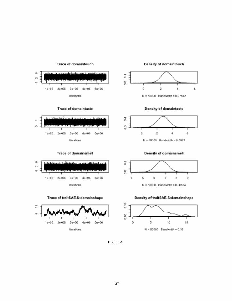
Figure 2:
137

Figure 3:
138

Figure 4:
139

Figure 5:
140

Figure 6:
141

Interpreting the results
Fixed effects estimates:sx.all = as.data.frame(summary(final.model)$solutions)apply(sx.all,2,signif,digits=3)
## post.mean l-95% CI u-95% CI eff.samp pMCMC## traitSAE.E -6.72 -7.490 -5.950 5200.0 0.00002## traitSAE.S -1.87 -2.590 -1.160 50000.0 0.00002## domainshape -5.31 -11.800 -0.189 15.6 0.00688## domainsound 1.78 0.639 2.880 9440.0 0.00264## domaintouch 2.69 1.370 3.940 12300.0 0.00024## domaintaste 2.78 1.270 4.310 15100.0 0.00080## domainsmell 6.69 5.570 7.750 10100.0 0.00002## traitSAE.S:domainshape 6.85 1.880 12.900 14.3 0.00002## traitSAE.S:domainsound -3.79 -4.200 -3.380 1460.0 0.00002## traitSAE.S:domaintouch -2.21 -2.630 -1.810 1460.0 0.00002## traitSAE.S:domaintaste -3.51 -3.970 -3.060 1910.0 0.00002## traitSAE.S:domainsmell -3.13 -3.460 -2.780 1140.0 0.00002
The results show that, across the board, abstract descriptions are more likely than source-based descriptions,which are more likely than evaluative descriptions. Compared to the colour domains, other domains are morelikely to use evaluative descriptions, except for shape which is more likely to use source-based descriptions. Theestimates for source-based descriptions of smell, sound, taste and touch are very similar, as are the estimatesfor evaluative descriptions for sound, taste and touch. However, the estimate for evaluative descriptions forsmell is much higher, suggesting that evaluative descriptions are more likely for the smell domain.
The graph below shows how the probaility of using Evaluative and Source-based descriptions differs from thebaseline condition, which is the sound domain. The vertical axis is in log probability, so above 0 means morelikely and below zero means less likely. If the 95% confidence intervals are different from 0, then there is asignificant effect. The difference in proportion of abstract responses for each domain (compared to colour) isimplied by the difference between the evaluative and source-based, and is plotted for ease of reference, but noconfidence intervals are given.
See the file results/SAE_interpretation.pdf for a fuller explanation of the results.
Note that the effective sample size (eff.samp) for two of the parameters is very low (< 100). These resultscome from increasing the number of iterations by an order of magnitude compared to the other models (toroughly two weeks processing time on a cluster computer). These increases made little difference to theeffective sample size, but did make the estimate distributions less bimodal. It is likely that a different priorwould help. However, the estimates are still significant, the outlying estimates suggest a greater effect size(not closer to zero) and the model fits the data well. We suggest that the differences are still significant. Alsonote that the model selection test preferred the interaction model even when all models were run for thesame number of iterations.plotModelEstimates = function(sx,ylab){
sx$var = rownames(sx)sx = sx[grepl("domain",sx$var),]sx$grp = "Evaluative"sx$grp[grepl("traitSAE\\.S",sx$var)] = "Source-based"
sx$domain = gsub("domain","",sx$var)sx$domain = gsub("traitSAE\\.S\\:","",sx$domain)
sx$var = substr(sx$var, 7,nchar(sx$var))
142

sx$var = factor(sx$var,levels = sae.order)names(sx)[names(sx)=="l-95% CI"] = 'lower'names(sx)[names(sx)=="u-95% CI"] = 'upper'
# add logical estimate of change for abstractsx = rbind(sx,
data.frame(post.mean = -(sx[1:5,1] + sx[6:10,1]),lower = rep(NA,5),upper = rep(NA,5),eff.samp = rep(NA,5),pMCMC = rep(NA,5),var = sx[1:5,]$var,grp = rep("Abstract",5),domain = sx[1:5,]$var
))
gx = ggplot(sx, aes(y=post.mean,x=domain, colour=grp)) +geom_hline(yintercept=0, color="black", size=1) +geom_point(size=3, position = position_dodge(width = 0.25)) +geom_errorbar(aes(ymax=upper,
ymin=lower),width=0.2,position = position_dodge(width=0.25))+
xlab("Domain")+ylab(ylab) +scale_color_manual(values=c("#619CFF", "#00BA38", "#F8766D"),name = "Description type")
return(gx)}
gx = plotModelEstimates(sx.all,"Difference from colour domain")gx
## Warning: Removed 5 rows containing missing values (geom_errorbar).
143

−10
−5
0
5
10
shape smell sound taste touch
Domain
Diff
eren
ce fr
om c
olou
r do
mai
n
Description type
Abstract
Evaluative
Source−based
pdf("../results/graphs/SAE_Results.pdf", height = 5)gx
## Warning: Removed 5 rows containing missing values (geom_errorbar).dev.off()
## pdf## 2
144

SAE model with alternative intercept
A model where the intercept is taste gives equivalent results:load("../results/SAE_mcmc_model_full_long_InterceptIsTaste.rdat")taste.model = m.mcmcglmmgx.taste = plotModelEstimates(as.data.frame(summary(taste.model)$solutions),
"Difference from taste domain")gx.taste
## Warning: Removed 5 rows containing missing values (geom_errorbar).
−10
0
10
20
colour shape smell sound touch
Domain
Diff
eren
ce fr
om ta
ste
dom
ain
Description type
Abstract
Evaluative
Source−based
pdf("../results/graphs/SAE_Results_InterceptIsTaste.pdf", height = 5)gx.taste
## Warning: Removed 5 rows containing missing values (geom_errorbar).dev.off()
## pdf## 2
145

Test differences between modalities
Are signed languages more likely to use particular types of response? Use a mixed effects model, predictinglikelihood of an abstract response, with random effects for language, consultant, domain, stimulus and theinteraction between language and domain. Then add a random effect for modality by domain, and a fixedeffect of modalityd$modality = "Spoken"d$modality[d$Language %in% c("ASL", "BSL", "Kata Kolok")] = "Signed"d$modality = factor(d$modality, levels=c("Spoken",'Signed'))dSignTest = d[d$domain!='sound',]dSignTest$domain = factor(dSignTest$domain)dSignTest$Language = factor(dSignTest$Language)dSignTest$Stimulus.code = factor(dSignTest$Stimulus.code)dSignTest$consultant = factor(dSignTest$consultant)dSignTest = dSignTest[complete.cases(dSignTest[,c("Language",'domain','SAE','consultant','Stimulus.code')]),]dSignTest$Abstract = dSignTest$SAE == "A"m0 = glmer(Abstract ~
1 +(1|Language/consultant) +(1|domain/Stimulus.code) +(1|Language:domain),
data = dSignTest,family = binomial)
m1 = update(m0,~.+(0 + modality|domain))m2 = update(m1,~.+modality)anova(m0,m1,m2)
## Data: dSignTest## Models:## m0: Abstract ~ 1 + (1 | Language/consultant) + (1 | domain/Stimulus.code) +## m0: (1 | Language:domain)## m1: Abstract ~ (1 | Language/consultant) + (1 | domain/Stimulus.code) +## m1: (1 | Language:domain) + (0 + modality | domain)## m2: Abstract ~ (1 | Language/consultant) + (1 | domain/Stimulus.code) +## m2: (1 | Language:domain) + (0 + modality | domain) + modality## Df AIC BIC logLik deviance Chisq Chi Df Pr(>Chisq)## m0 6 24556 24606 -12272 24544## m1 9 24558 24633 -12270 24540 3.9828 3 0.2633## m2 10 24560 24642 -12270 24540 0.4999 1 0.4796
Neither the fixed effect of modality nor the random effect of modality by domain improves the model. Thatis, signed languages are not a distinct group.
146

Test if abstract responses are less likely in later descriptions.
Respondents could produce multiple responses. In conversational interaction, participants tend to movetowards more specific information when converging on a referent of a description (Dingemanse et al., 2015).Abstract responses are proportionately less likely in later descriptions:d = d.all # switch back to all responses# Recode categories to plotd$Response.cat = "1"d[d$Response==2,]$Response.cat = "2"d[d$Response==3,]$Response.cat = "3"d[d$Response==4,]$Response.cat = "4"d[d$Response>4,]$Response.cat = "5+"
txR = melt(prop.table(table(d$SAE,d$Response.cat),2))
ggplot(txR,aes(x = Var2, y = value,fill = Var1)) +geom_bar(position = "fill",stat = "identity") +scale_y_continuous(labels = percent_format()) +xlab("Response Number") + ylab("Percentage of responses")
0%
25%
50%
75%
100%
1 2 3 4 5+
Response Number
Per
cent
age
of r
espo
nses
Var1
A
E
S
We test whether the probability of using an abstract description varies according to the number of times thatstimuli had been named by the respondent previously. Response numbers range from 1 to 15, but 99% are 5or lower. We set all response numbers of 5 or more to be equal to 5. We used a linear mixed effects modelwith random intercepts for respondent within languages and stimuli within domains, with a random slope forresponse number by domain.
We compare a model with random intercepts for consultants within languages and stimuli within domain.
147

Then a third model adds the main effect for response number.logit2prob=function(X){
exp(X)/(1+exp(X))}
d$SAE.abstract = d$SAE=="A"d$Response2 = d$Responsed$Response2[d$Response>5]=5d$Response2 = d$Response2-1
m0 = glmer(SAE.abstract~ 1 +(1|Language/consultant) +(1|domain/Stimulus.code),
data = d,family='binomial')
mR = glmer(SAE.abstract~ 1 +(1|Language/consultant) +(1|domain/Stimulus.code) +(0+Response2|domain),data = d,family='binomial')
mRD = glmer(SAE.abstract~ Response2 +(1|Language/consultant) +(1|domain/Stimulus.code) +(0+Response2|domain),data = d,family='binomial')
ax = anova(m0,mR,mRD)ax
## Data: d## Models:## m0: SAE.abstract ~ 1 + (1 | Language/consultant) + (1 | domain/Stimulus.code)## mR: SAE.abstract ~ 1 + (1 | Language/consultant) + (1 | domain/Stimulus.code) +## mR: (0 + Response2 | domain)## mRD: SAE.abstract ~ Response2 + (1 | Language/consultant) + (1 | domain/Stimulus.code) +## mRD: (0 + Response2 | domain)## Df AIC BIC logLik deviance Chisq Chi Df Pr(>Chisq)## m0 5 40039 40083 -20015 40029## mR 6 39820 39872 -19904 39808 221.076 1 <2e-16 ***## mRD 7 39821 39881 -19904 39807 1.408 1 0.2354## ---## Signif. codes: 0 '***' 0.001 '**' 0.01 '*' 0.05 '.' 0.1 ' ' 1summary(mRD)
## Generalized linear mixed model fit by maximum likelihood (Laplace## Approximation) [glmerMod]## Family: binomial ( logit )## Formula:## SAE.abstract ~ Response2 + (1 | Language/consultant) + (1 | domain/Stimulus.code) +## (0 + Response2 | domain)
148

## Data: d#### AIC BIC logLik deviance df.resid## 39820.9 39881.4 -19903.5 39806.9 41592#### Scaled residuals:## Min 1Q Median 3Q Max## -9.5246 -0.5257 0.3216 0.5305 7.3251#### Random effects:## Groups Name Variance Std.Dev.## consultant.Language (Intercept) 0.65725 0.8107## Stimulus.code.domain (Intercept) 0.32418 0.5694## Language (Intercept) 0.55582 0.7455## domain Response2 0.05305 0.2303## domain.1 (Intercept) 1.62350 1.2742## Number of obs: 41599, groups:## consultant:Language, 313; Stimulus.code:domain, 147; Language, 20; domain, 6#### Fixed effects:## Estimate Std. Error z value Pr(>|z|)## (Intercept) 0.84131 0.55340 1.520 0.128## Response2 -0.12239 0.09648 -1.269 0.205#### Correlation of Fixed Effects:## (Intr)## Response2 -0.003# estimated probability at first response:pA.R1 = logit2prob(fixef(mRD)[1])# probability decrease with each response:pA.Rplus = pA.R1 - logit2prob(sum(fixef(mRD)))
#The probability of producing an abstract response in the first turn isround(pA.R1*100,1)
## (Intercept)## 69.9# % . This decreases byround(pA.Rplus*100,1)
## (Intercept)## 2.6#percentage points after each response.
Random slopes for response number by domain significantly improve the fit of the model. Abstract descriptionsare not less likely in later descriptions when controlling for this random slope. That is, the effect is strongerfor some domains:rint = fixef(mRD)[1] + ranef(mRD)$domain[,1]rslope = fixef(mRD)[2] + ranef(mRD)$domain[,1]
xpoints = seq(1,5,length.out=100)
dx = data.frame(
149
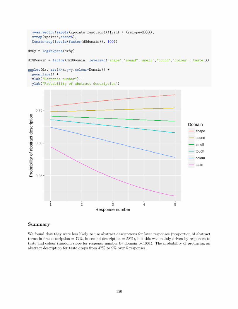
y=as.vector(sapply(xpoints,function(X){rint + (rslope*X)})),x=rep(xpoints,each=6),Domain=rep(levels(factor(d$domain)), 100))
dx$y = logit2prob(dx$y)
dx$Domain = factor(dx$Domain, levels=c("shape","sound",'smell',"touch",'colour','taste'))
ggplot(dx, aes(x=x,y=y,colour=Domain)) +geom_line() +xlab("Response number") +ylab("Probability of abstract description")
0.25
0.50
0.75
1 2 3 4 5
Response number
Pro
babi
lity
of a
bstr
act d
escr
iptio
n
Domain
shape
sound
smell
touch
colour
taste
Summary
We found that they were less likely to use abstract descriptions for later responses (proportion of abstractterms in first description = 72%, in second description = 58%), but this was mainly driven by responses totaste and colour (random slope for response number by domain p<.001). The probability of producing anabstract description for taste drops from 47% to 9% over 5 responses.
150


![Stochastic homogenization of subdi erential inclusions …veneroni/stochastic.pdf · Stochastic homogenization of subdi erential inclusions via scale integration Marco ... 32], Bensoussan,](https://img.pdfslide.tips/doc/110x75/5b7c19bc7f8b9a9d078b9b97/stochastic-homogenization-of-subdi-erential-inclusions-veneroni-stochastic.jpg)