TABLE OF CONTENTS

SolarSOHO EIT 195 …………………………………………………………………………………………… 1Solar radio bursts ………………………………………………………….................................................... 2STEREO WAVES …………………………………………………………………………………………… 3ACE Channels – travel times ………………………………………….................................................... 4Diagnosing prompt flare particles …………………………………………………………………………… 5Solar magnetogram + magnetic connection (WSA, ENLIL) …………………………………………… 6Carrington coordinates …………………………………………………………………………………………… 7Synoptic maps …………………………………………………………………………………………… 8Synoptic magnetograms – carrington coordinates ……………………………………………………… 9-12

HeliosphereSOHO LASCO C3 ……………………………………………………………………..……………….. 13SOHO LASCO C3 Running Difference ………………………………………………………………………. 14Enlil Cone Model Input ………………………………………………………………………………………. 15Enlil Solar Wind at L1 (24 hours history) ………………………………………………………………………. 16Enlil Solar Wind at L1 (48 hours prediction ………………………………………………………………………. 17

Magnetosphere/IonosphereSWMF (Gombosi et al.) driven by ACE or Enlil cone model solar wind. ………………………………………. 18

Visualization of the state of the magnetosphere ……………………………………………………. 19 Density, velocity and magnetic field (north-south cut) ……………………………………………………. 20 Magnetopause position (equatorial cut) ……………………………………………………………………. 21 Magnetopause standoff ……………………………………………………………………………………. 22 Polar cap boundary ……………………………………………………………………………………. 23 Ionospheric field-aligned currents and polar cap ……………………………………………………. 24 Polar cap size ……………………………………………………………………………………. 24 Joule dissipation in ionosphere ……………………………………………………. 25 Cross cap ionospheric potential difference ……………………………………………………. 26 Ring current equatorial H+ fluxes at 61.2KeV, 138.6KeV, 300KeV ……………………………………. 27 Ring current H+ fluxes at LANL-02A …………………………………………………….. 27 Global geomagnetically induced currents (GIC) proxy …………………………………….. 28 Geomagnetically induced total electric field …………………………………………………….. 29SWMF driven by Enlil cone model solar wind: Summary of predicted parameters …………………...... 30Radiation belt e- fluxes at 100keV, 1000keV, 4000keV (Fok Radiation Belt Model) ................................... 31RBSP will measure particle fluxes from 600 km to GEO …………………………………….. 32Energetic particles at LANL (RBSP will measure ion and electron flux within GEO) …………………….. 33AE index …………………………………………………………………………………….. 34DEMETER (C/NOFS will observe electron density irregularities) ………………………………….. 35TIMED GUVI measures auroral precipitation …………………………………………………….. 36 Global Ionosphere Models …………………………………………………………………….. 37USU-GAIM TEC …………………………………………………………………………………….. 38Absorption values for 5 and 10 MHz HF signals (AbbyNormal) …………………………………….. 39C/NOFS (Electron number density Ne, TEC, NmF2, HmF2) …………………………………….. 40C/NOFS (Neutral densities) …………………………………………………………………….. 40

SOHO EIT 195

-1-

Solar Radio Bursts – Corona to 1 AU

-2-

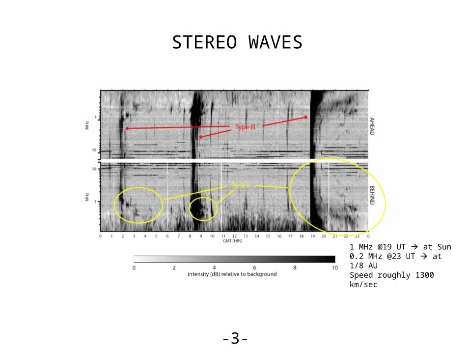
1 MHz @19 UT at Sun0.2 MHz @23 UT at 1/8 AUSpeed roughly 1300 km/sec

STEREO WAVES

-3-

ACE Channels – Travel Times (Very Approxmate)

-4-

Diagnosing Prompt Flare Particles

-5-

Solar magnetogram + magnetic connection (WSA, ENLIL)

• The sun’s surface magnetic field and an estimate of the footpoints of the fieldlines connecting the 4 inner planets to the sun at a specific time. (Earth is *)

• Field map is synoptic and in Carrington Coordinates!

-6-

Carrington Coordinates

• Sun is gaseous and rotating – no fixed point on which to attach a coordinate origin.

• Carrington introduced a spherical coordinate system rotating with a 25.38 day rotation period for tracking sunspot motions.

• He identified the sub-earth solar line of longitude, early on afternoon of Nov. 9, 1853 as longitude zero and Rotation number 0

• Each rotation begins at longitude 360 and ends at longitude 0

– note (CR=0, = 0 is the same longitude as CR=1, = 360).

• Current definition is more systematic and obtuse– Uses rotation rate of 27.2753 days

– The canonical zero meridian is the one that passed through the ascending node of the solar equator on the ecliptic at Greenwich mean noon January 1, 1854.

To earth, Nov 9, 1853

= 0, CR=0

= 360, CR=1

-7-

Synoptic Maps

• Synoptic maps are constructed by combining front side observations over a full rotation

• The point on sun directly below earth moves from right to left with time in a given map.

• In maps made on successive days, a given feature (eg a sunspot) moves to the right with the solar rotation.

Time

Direction of feature rotation

-8-

Synoptic Magnetograms – Carrington Coords

-90

90

0

-60 +60 0

1X

90

-90

-60 +60

Select 120o window about central meridian

Remap window and multiply data in window by a longitude-dependent weighting function

Place result in cartesian (carrington longitude, latitude) plot

-9-

Synoptic Magnetograms – Carrington Coords

90

-90

eg Day 21 Day 14 Day 8

Carrington Longitude

-10-

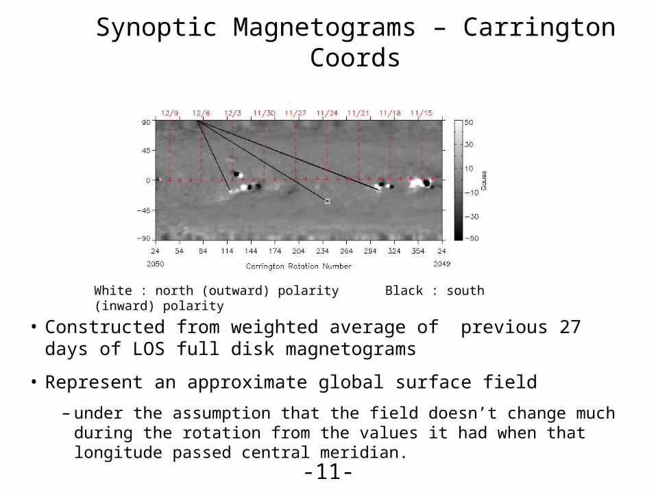
Synoptic Magnetograms – Carrington Coords

• Constructed from weighted average of previous 27 days of LOS full disk magnetograms

• Represent an approximate global surface field

– under the assumption that the field doesn’t change much during the rotation from the values it had when that longitude passed central meridian.

White : north (outward) polarity Black : south (inward) polarity

-11-

Synoptic Magnetograms – Carrington Coords

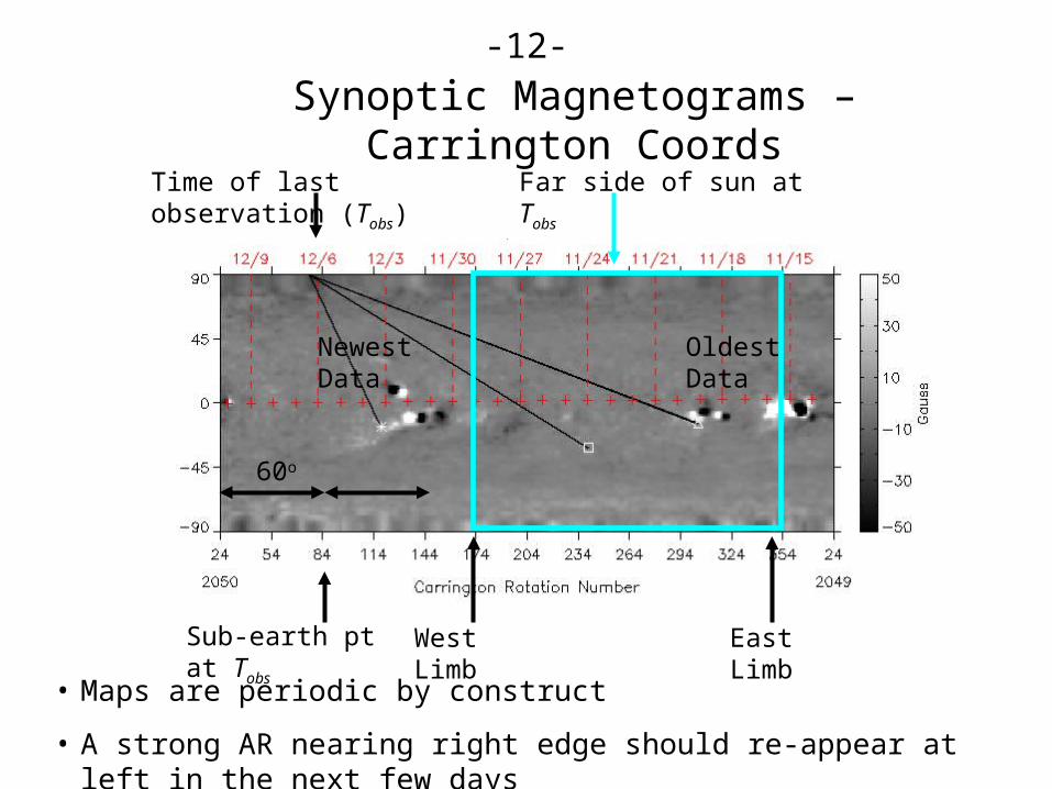
• Maps are periodic by construct

• A strong AR nearing right edge should re-appear at left in the next few days

Time of last observation (Tobs)

60o

Far side of sun at Tobs

West Limb East Limb

Oldest DataNewest Data

Sub-earth pt at Tobs

-12-

SOHO LASCO C3

-13-

Running difference images are usually made by subtracting from each image the one preceding it. Thus, moving fronts look white with black trailing edges. This highlights changes and moving features.

SOHO LASCO C3 Running Difference

-14-

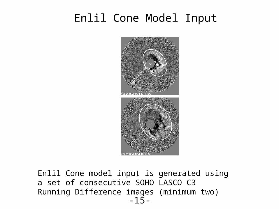
Enlil Cone model input is generated using a set of consecutive SOHO LASCO C3 Running Difference images (minimum two)

Enlil Cone Model Input

-15-

Enlil Solar Wind at L1 (24 hours history)

The model ‘nowcast’ (last 24 hours) for solar wind electron number density, speed and ‘magnetic polarity’ at Earth.

N

-Vr

Sign( Br )

-16

Enlil Solar Wind at L1 (48 hours prediction)

The model 48 hour forecast for solar wind mass density, speed and ‘magnetic polarity’ at Earth.

N

-Vr

Sign( Br )

-17-

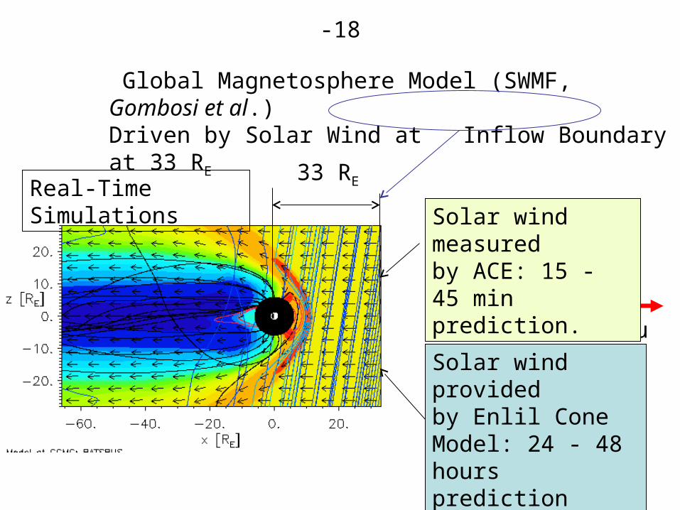
Sun

33 RE

Solar wind provided by Enlil Cone Model: 24 - 48 hours prediction (during Halo CME only)

Global Magnetosphere Model (SWMF, Gombosi et al.) Driven by Solar Wind at Inflow Boundary at 33 RE

Solar wind measuredby ACE: 15 - 45 min prediction.

Real-Time Simulations

-18

Visualization of the State of the Magnetosphere

• 2D slices (north-south cut, equatorial cut, lat-long maps)– 24 hours history movies (end at the release time)

– 24 hours movies ahead of real time (end 15-45 min after the release time)

– 48 hours prediction movies (start at the release time)

• Time evolution of parameters characterizing the state of the magnetosphere/ionosphere

– 24 hours history plots (end at the release time)

– 24 hours plots (end 15-45 min after the release time)

– 48 hours prediction plots (start at the release time)

-19-

Overview of the Global State of the Magnetosphere: Density, Velocity and Magnetic Field (North-South Cut)

Density (color, log scale), Velocity (vectors),Magnetic field (lines)

Quiet magnetopshere

Magnetopshere hit by CME

Substorm onset

reconnection onset

Near-earth reconnection causes energetic particle injection at geosynch. orbit, drive geomagnetically induced currents.

-20-

Magnetopause Position (Equatorial Cut)

Quiet magnetopshere

Magnetopause within 1 RE of the geosynch. orbit

Magnetopause cross the geosynch. orbit

magnetopause position

geosynch. orbit

GOES 11&12

-21-

Magnetopause Standoff

magnetopause position: projection of boundary between open and closed field lines on equatorial plane

geosynch. orbit

magnetopause standoff distance

Magnetopause Standoff Evolution with Time

Time

geosynch. orbit

-22-

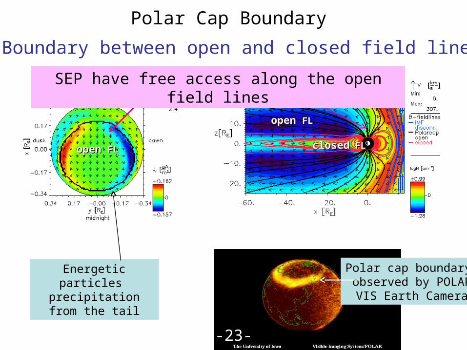
open open FLFL

Polar cap boundary observed by POLARVIS Earth Camera

Polar Cap Boundary

Boundary between open and closed field lines

open open FLFL

closedclosed FL FL

SEP have free access along the open field lines

Energetic particles precipitation from the

tail

-23-

Ionospheric Field-Aligned Currents and Polar Cap

Polar Cap Size Evolution with Time

Time

Quiet Time Storm Time

-24-

Joule Dissipation in the Ionosphere

Joule Dissipation in the Ionosphere Time Evolution

Quiet: < 100 GW

Moderate: 100 - 200 GW

Jdiss Jr ds

Storm: > 400 GW

Time

Ionospheric Potential

Radial Current

surface integral

Northern Hemisphere

Sourthern Hemisphere

-25-

Cross Cap Ionospheric Potential Difference

Cross Cap Ionospheric Time Evolution

Time

Quiet: < 75 keV

Moderate: 100 - 150 keV

maxmin

max

min

min max

Storm: > 250 keV

Large affect densitydistribution in ionosphere, drive GIC

Northern Hemisphere

Sourthern Hemisphere

-26-

Fok Ring Current Model Driven by SWMF: Equatorial H+ fluxes

61.2KeV 138.6KeV 300KeV

Ring current H+ fluxes at LANL-02A geosynch. satellite

Substorm injection at geosynch. orbit

Time

Quiet

Storm

geosynch. orbit

-27-

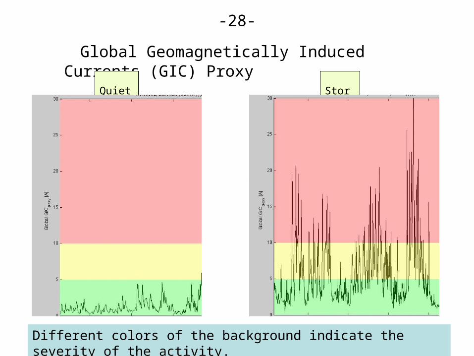
Global Geomagnetically Induced Currents (GIC) Proxy

Quiet Storm

Different colors of the background indicate the severity of the activity.

-28-

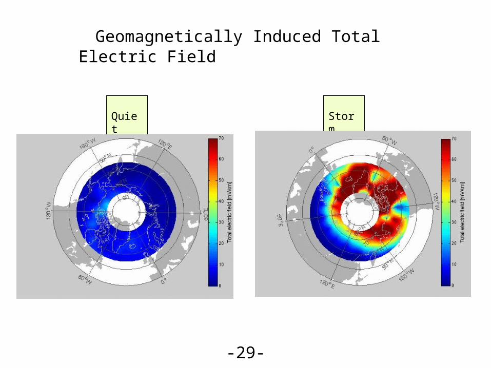
Geomagnetically Induced Total Electric Field

Quiet Storm

-29-

SWMF Driven by Solar Wind Modeled by Enlil: Predicted Parameters Characterizing Global State

of the Magnetosphere/Ionosphere

• Time of geomagnetic activity onset

• Duration of severe geomagnetic activity

• Magnitude of geomagnetic activity

– Magnetopause cross/touch/approach geosynch. orbit

– Max value of Joule dissipation

– Max value of polar cap size

– Max value of cross cap ionospheric potential difference

– Max GIE and GIC

– Max particle fluxes

24-48 hours prediction, 10-20 % uncertainty

Opportunities for comparison SWMF driven by Enlil SW (24- 48 hours prediction) with SWMF driven by ACE SW (15 – 45 min prediction).

-30-

Fok Radiation Belt Model: Equatorial e- Fluxes

100 KeV 1 MeV 4 Mev

100 KeV 1 MeV 4 Mev

Quiet

Storm

geosynch. orbit

-31-

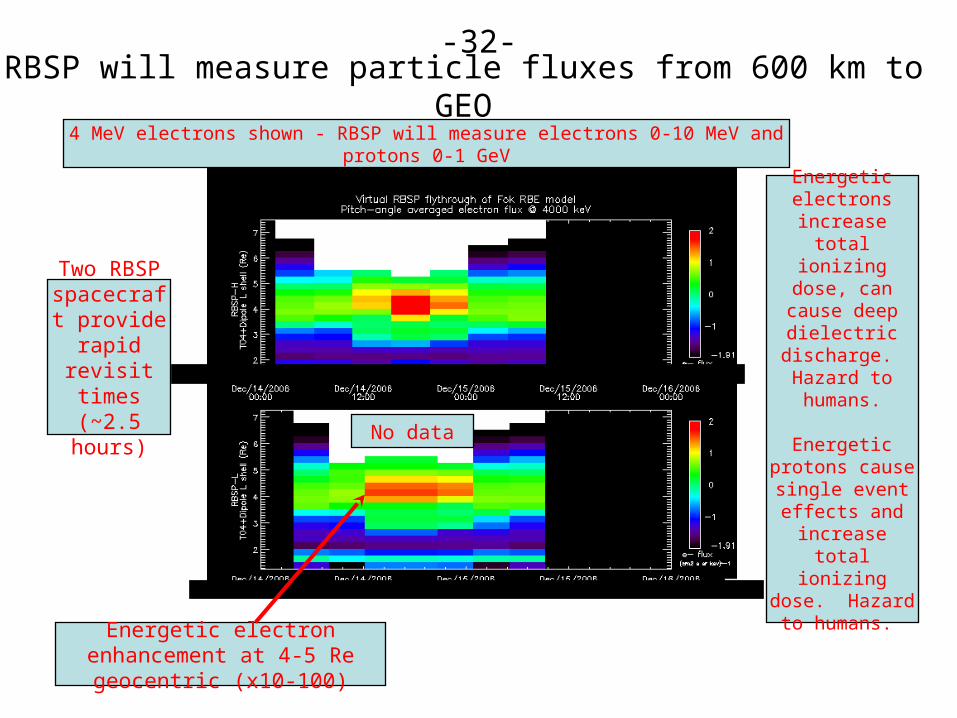
RBSP will measure particle fluxes from 600 km to GEO

Energetic electron enhancement at 4-5 Re

geocentric (x10-100)

Two RBSP spacecraft

provide rapid revisit times(~2.5 hours)

Energetic electrons

increase total ionizing dose,

can cause deep dielectric

discharge. Hazard to humans.

Energetic protons cause single event effects and

increase total ionizing dose.

Hazard to humans.

No data

4 MeV electrons shown - RBSP will measure electrons 0-10 MeV and protons 0-1 GeV

-32-

RBSP will measure ion and electron flux within GEO

Quiet interv

al

Substorm

onsets

Substorms inject

energetic particles

within GEO, causing

spacecraft charging

Shock arrival -33-

Substorm onsets

Quiet interval

Substorms cause increased ionization and energy deposition at high latitudes -

increase neutral density and interfere with HF communications

Substorms also inject energetic electrons and ions at geosynchronous orbit, resulting

in spacecraft charging, sometimes to hundreds or thousands of volts

Auroral Electrojet indices show substorm onsets

-34-

C/NOFS will observe electron density irregularities

Day 1 Day 5Day 2 Day 4 Day 6Day 3

Density irregularities interfere with NAV /

COMM signals

Changes in background electron

density affect HF communication /

propagation paths

-35-

TIMED GUVI measures auroral precipitation

TIMED GUVI measures E0

(characteristic precipitating

electron energy)

and energy flux

TIMED GUVI shows size of polar cap, and data can be

used to feed predictive models

of ionization, convection, etc.

Enhanced ionization

interferes with HF communication.

At low-latitudes, GUVI also

measures airglow / electron density. Can be used to assess bubble formation and

irregularity generation.

Quiet interval

-36-

Global Ionosphere Models

Global Assimilation of Ionospheric Measurements (USU-GAIM, Schunk et al.)

USU-GAIM uses a physics-based Ionosphere Forecast Model (IFM).

USU-GAIM assimilates electron density (Ne) profiles from a diverse set of real-time (or near real-time) measurements: - slant TEC from GPS ground stations via RINEX files,

- bias information for GPS satellites and ground-stations,- electron density profiles from DISS ionosondes via SAO files

AbbyNormal Model (Eccles et al., Space Environment Corporation) calculates absorption values for HF signals

Ionosphere Forecast Model (IFM) needs - F10.7, daily Ap, 3-hour Kp indices

` - neutral wind, electric field, auroral precipitation, solar EUV (empirical inputs)

-37-

USU-GAIM Model: Total Electron Content (TEC)

Normal TEC

Increased TEC

-38-

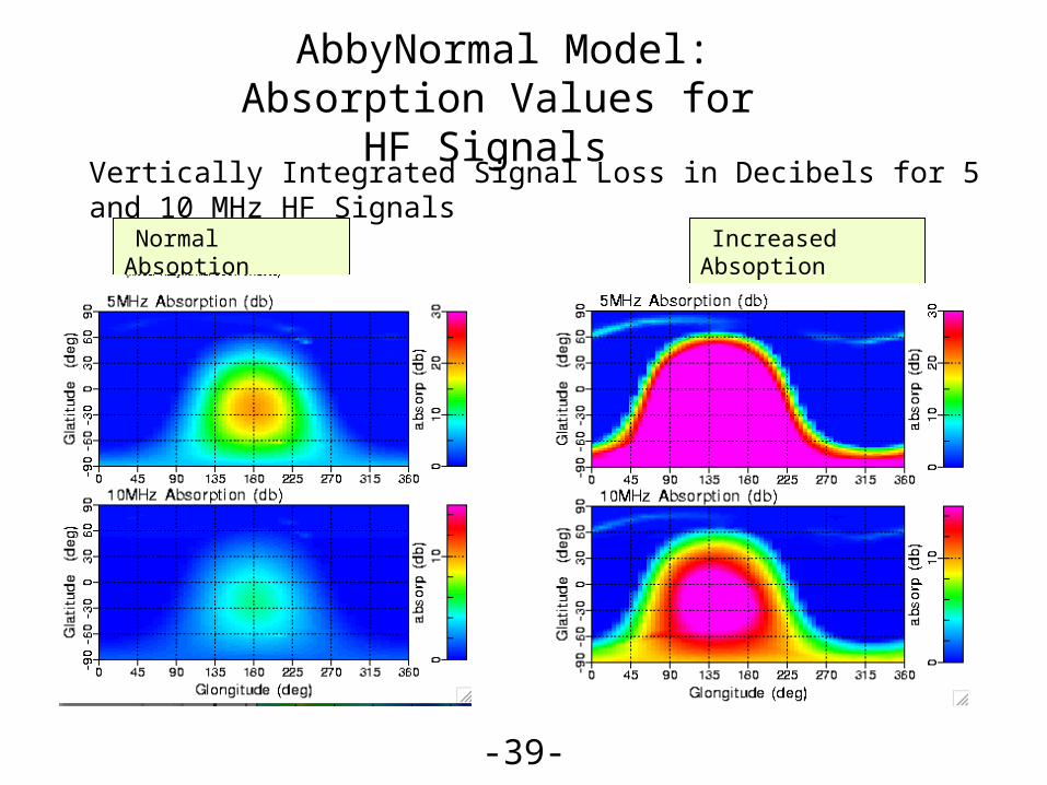
AbbyNormal Model: Absorption Values for HF Signals

Normal Absoption

Vertically Integrated Signal Loss in Decibels for 5 and 10 MHz HF Signals

Increased Absoption

-39-

C/NOFS measures neutral, plasma densityand electron density profiles

C/NOFS measures neutral densities (dashed line shows quiet value) and in situ electron density, as well as density profiles.

Abrupt gradients in electron density provide conditions suitable for electron density irregularity formation.Changing TEC, HMF2, NMF2 interfere with NAV/COMM signals

Typical quiet time neutral density at

perigee

-40-