Embed Size (px)
Citation preview
Techniques of GPD extraction from data
Kresimir Kumericki
University of Zagreb, Croatia
INT-17-3 Workshop: Tomography of Hadrons and Nuclei at Jefferson LabAugust 28 – September 29, 2017
Seattle, WA
Introduction — DVCS φ vs. harmonics Global fits Neural nets Conclusion
Outline
Introduction — DVCS
φ vs. harmonics
Global fits
Neural nets
Conclusion
2 Kresimir Kumericki : GPD extraction
Introduction — DVCS φ vs. harmonics Global fits Neural nets Conclusion
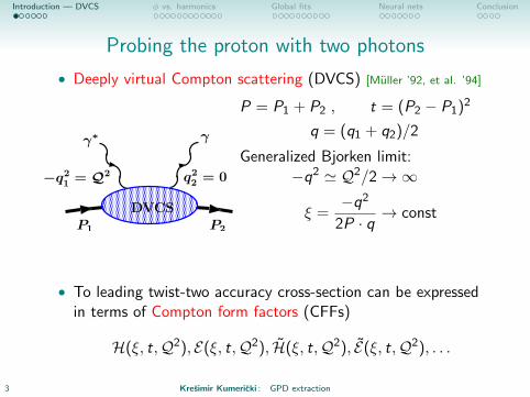
Probing the proton with two photons
• Deeply virtual Compton scattering (DVCS) [Muller ’92, et al. ’94]
γ∗
P1 P2
DVCS
−q2
1= Q2 q2
2= 0
γ
P = P1 + P2 , t = (P2 − P1)2
q = (q1 + q2)/2
Generalized Bjorken limit:
−q2 ' Q2/2→∞
ξ =−q2
2P · q → const
• To leading twist-two accuracy cross-section can be expressedin terms of Compton form factors (CFFs)
H(ξ, t,Q2), E(ξ, t,Q2), H(ξ, t,Q2), E(ξ, t,Q2), . . .
3 Kresimir Kumericki : GPD extraction
Introduction — DVCS φ vs. harmonics Global fits Neural nets Conclusion
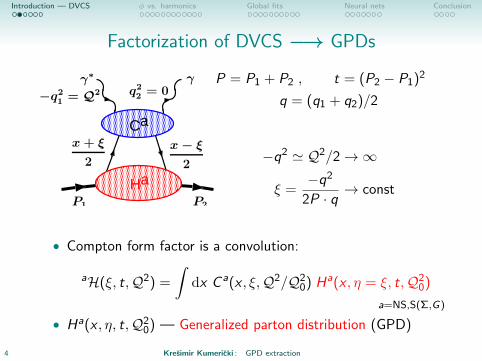
Factorization of DVCS −→ GPDs
γ∗
P1 P2
−q21 = Q2 q2
2 = 0γ
x + ξ
2
x − ξ
2
Ha
Ca
P = P1 + P2 , t = (P2 − P1)2
q = (q1 + q2)/2
−q2 ' Q2/2→∞
ξ =−q2
2P · q → const
• Compton form factor is a convolution:
aH(ξ, t,Q2) =
∫dx C a(x , ξ,Q2/Q2
0) Ha(x , η = ξ, t,Q20)
a=NS,S(Σ,G)
• Ha(x , η, t,Q20) — Generalized parton distribution (GPD)
4 Kresimir Kumericki : GPD extraction
Introduction — DVCS φ vs. harmonics Global fits Neural nets Conclusion
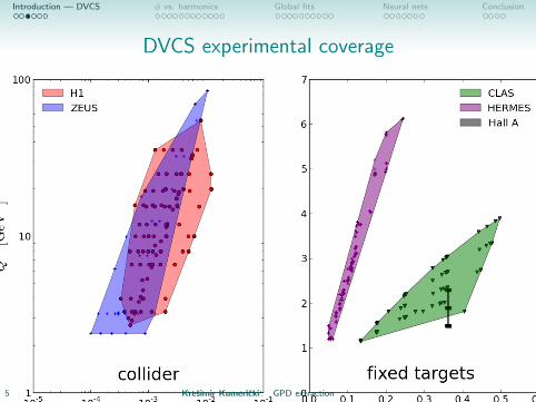
DVCS experimental coverage
• COMPASS II, JLAB@12 and EIC to fill in the gaps
5 Kresimir Kumericki : GPD extraction
Introduction — DVCS φ vs. harmonics Global fits Neural nets Conclusion
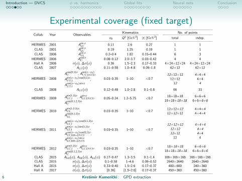
Experimental coverage (fixed target)
Collab. Year ObservablesKinematics No. of points
xB Q2 [GeV2] |t| [GeV2] total indep.
HERMES 2001 AsinφLU 0.11 2.6 0.27 1 1
CLAS 2001 AsinφLU 0.19 1.25 0.19 1 1
CLAS 2006 AsinφUL 0.2–0.4 1.82 0.15–0.44 6 3
HERMES 2006 AcosφC 0.08–0.12 2.0–3.7 0.03–0.42 4 4
Hall A 2006 σ(φ), ∆σ(φ) 0.36 1.5–2.3 0.17–0.33 4×24+12×24 4×24+12×24CLAS 2007 ALU(φ) 0.11–0.58 1.0–4.8 0.09–1.8 62×12 62×12
HERMES 2008
Acos(0,1)φC , A
sin(φ−φS )UT,DVCS,
Asin(φ−φS ) cos(0,1)φUT,I ,
Acos(φ−φS ) sinφUT,I
0.03–0.35 1–10 <0.712+12+12
12+1212
4+4+44+44
CLAS 2008 ALU(φ) 0.12–0.48 1.0–2.8 0.1–0.8 66 33
HERMES 2009 Asin(1,2)φLU,I , Asinφ
LU,DVCS,
Acos(0,1,2,3)φC
0.05–0.24 1.2–5.75 <0.718+18+18
18+18+18+186+6+6
6+6+6+6
HERMES 2010 Asin(1,2,3)φUL ,
Acos(0,1,2)φLL
0.03–0.35 1–10 <0.712+12+1212+12+12
4+4+44+4+4
HERMES 2011
Acos(φ−φS ) cos(0,1,2)φLT,I ,
Asin(φ−φS ) sin(1,2)φLT,I ,
Acos(φ−φS ) cos(0,1)φLT,BH+DVCS ,
Asin(φ−φS ) sinφLT,BH+DVCS
0.03–0.35 1–10 <0.7
12+12+1212+1212+12
12
4+4+44+44+4
4
HERMES 2012 Asin(1,2)φLU,I , Asinφ
LU,DVCS,
Acos(0,1,2,3)φC
0.03–0.35 1–10 <0.718+18+18
18+18+18+186+6+6
6+6+6+6
CLAS 2015 ALU(φ), AUL(φ), ALL(φ) 0.17–0.47 1.3–3.5 0.1–1.4 166+166+166 166+166+166CLAS 2015 σ(φ), ∆σ(φ) 0.1–0.58 1–4.6 0.09–0.52 2640+2640 2640+2640Hall A 2015 σ(φ), ∆σ(φ) 0.33–0.40 1.5–2.6 0.17–0.37 480+600 240+360Hall A 2017 σ(φ), ∆σ(φ) [0.36] [1.5–2.0] 0.17–0.37 450+360 450+360
6 Kresimir Kumericki : GPD extraction
Introduction — DVCS φ vs. harmonics Global fits Neural nets Conclusion
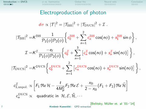
Electroproduction of photon
dσ ∝ |T |2 = |TBH|2 + |TDVCS|2 + I .
|TBH|2 =KBH 1
P1(φ)P2(φ)
{cBH
0 +2∑
n=1
cBHn cos(nφ) + sBH
1 sinφ
},
I =KI−e`
P1(φ)P2(φ)
{cI0 +
3∑n=1
[cIn cos(nφ) + sIn sin(nφ)
]},
|TDVCS|2 =KDVCS
{cDVCS
0 +2∑
n=1
[cDVCSn cos(nφ) + sDVCS
n sin(nφ)]}
,
cI1,unpol. ∝[F1 ReH− t
4M2p
F2 Re E +xB
2− xB(F1 + F2)Re H
]cDVCSn ∝ quadratic in H, E , H, · · ·
[Belitsky, Muller et. al ’01–’14]7 Kresimir Kumericki : GPD extraction
Introduction — DVCS φ vs. harmonics Global fits Neural nets Conclusion
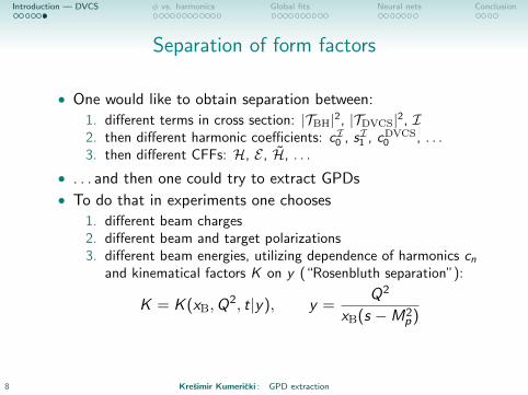
Separation of form factors
• One would like to obtain separation between:
1. different terms in cross section: |TBH|2, |TDVCS|2, I2. then different harmonic coefficients: cI0 , sI1 , cDVCS
0 , . . .3. then different CFFs: H, E , H, . . .
• . . . and then one could try to extract GPDs
• To do that in experiments one chooses
1. different beam charges2. different beam and target polarizations3. different beam energies, utilizing dependence of harmonics cn
and kinematical factors K on y (“Rosenbluth separation”):
K = K (xB,Q2, t|y), y =
Q2
xB(s −M2p)
8 Kresimir Kumericki : GPD extraction
Introduction — DVCS φ vs. harmonics Global fits Neural nets Conclusion
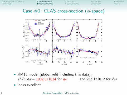
Case #1: CLAS cross-section (φ-space)
0.00
0.05
0.10
0.15
0.20
0.25
0.30
dσ
=dσ←
+dσ→
xB = 0.335, Q2 = 2.78, t = -0.2
KM15 prelim.
KMM12
CLAS 2015
xB = 0.335, Q2 = 2.78, t = -0.26 xB = 0.335, Q2 = 2.78, t = -0.45
0 100 200 300 400
φ [deg]
0.10
0.05
0.00
0.05
0.10
∆σ
=dσ←−dσ→
xB = 0.335, Q2 = 2.78, t = -0.2
0 100 200 300 400
φ [deg]
xB = 0.335, Q2 = 2.78, t = -0.26
0 100 200 300 400
φ [deg]
xB = 0.335, Q2 = 2.78, t = -0.45
• KM15 model (global refit including this data):χ2/npts = 1032.0/1014 for dσ and 936.1/1012 for ∆σ
• looks excellent
9 Kresimir Kumericki : GPD extraction
Introduction — DVCS φ vs. harmonics Global fits Neural nets Conclusion
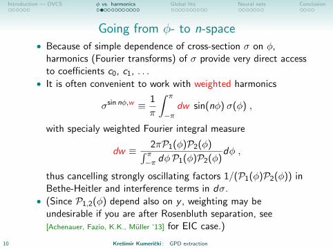
Going from φ- to n-space• Because of simple dependence of cross-section σ on φ,
harmonics (Fourier transforms) of σ provide very direct accessto coefficients c0, c1, . . .
• It is often convenient to work with weighted harmonics
σsin nφ,w ≡ 1
π
∫ π
−πdw sin(nφ) σ(φ) ,
with specialy weighted Fourier integral measure
dw ≡ 2πP1(φ)P2(φ)∫ π−π dφP1(φ)P2(φ)
dφ ,
thus cancelling strongly oscillating factors 1/(P1(φ)P2(φ)) inBethe-Heitler and interference terms in dσ.
• (Since P1,2(φ) depend also on y , weighting may beundesirable if you are after Rosenbluth separation, see[Achenauer, Fazio, K.K., Muller ‘13] for EIC case.)
10 Kresimir Kumericki : GPD extraction
Introduction — DVCS φ vs. harmonics Global fits Neural nets Conclusion
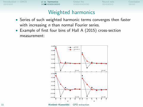
Weighted harmonics• Series of such weighted harmonic terms converges then faster
with increasing n than normal Fourier series.• Example of first four bins of Hall A (2015) cross-section
measurement:
n
0.02
0.00
0.02
0.04
0.06
0.08
bin #1
cos(n )
cos(n ), w
nbin #2
0 1 2 3 4 5n
0.02
0.01
0.00
0.01
0.02
0.03
0.04
bin #30 1 2 3 4 5
n
bin #4
11 Kresimir Kumericki : GPD extraction

Introduction — DVCS φ vs. harmonics Global fits Neural nets Conclusion
Case #1: CLAS cross-section (n-space)
0.00
0.05
0.10
0.15
0.20
0.25
0.30
0.35
0.40
∆σ
sinφ,w
Q2 =1.63xB =0.18
Q2 =1.64xB =0.21
Q2 =1.88xB =0.21
Q2 =1.79xB =0.24
Q2 =2.12xB =0.24
0.1 0.2 0.3 0.4 0.50.00
0.01
0.02
0.03
0.04
0.05
0.06
∆σ
sinφ,w
Q2 =2.35xB =0.28
0.1 0.2 0.3 0.4 0.5
Q2 =2.58xB =0.30
0.1 0.2 0.3 0.4 0.5
−t [GeV2 ]
Q2 =2.78xB =0.34
0.1 0.2 0.3 0.4 0.5
Q2 =2.97xB =0.36
0.1 0.2 0.3 0.4 0.5
Q2 =3.18xB =0.40
0.0
0.2
0.4
0.6
0.8
1.0
1.2
1.4
1.6
dσ
cos0φ,w
Q2 =1.63xB =0.18
Q2 =1.64xB =0.21
Q2 =1.88xB =0.21
Q2 =1.79xB =0.24
Q2 =2.12xB =0.24
0.1 0.2 0.3 0.4 0.50.00
0.05
0.10
0.15
0.20
dσ
cos0φ,w
Q2 =2.35xB =0.28
0.1 0.2 0.3 0.4 0.5
Q2 =2.58xB =0.30
0.1 0.2 0.3 0.4 0.5
−t [GeV2 ]
Q2 =2.78xB =0.34
0.1 0.2 0.3 0.4 0.5
Q2 =2.97xB =0.36
0.1 0.2 0.3 0.4 0.5
Q2 =3.18xB =0.40
0.4
0.3
0.2
0.1
0.0
0.1
dσ
cosφ,w
Q2 =1.63xB =0.185
Q2 =1.64xB =0.214
Q2 =1.88xB =0.215
Q2 =1.79xB =0.244
Q2 =2.12xB =0.245
0.1 0.2 0.3 0.4 0.50.05
0.04
0.03
0.02
0.01
0.00
0.01
0.02
0.03
dσ
cosφ,w
Q2 =2.35xB =0.275
0.1 0.2 0.3 0.4 0.5
Q2 =2.58xB =0.305
0.1 0.2 0.3 0.4 0.5
−t [GeV2 ]
Q2 =2.78xB =0.335
0.1 0.2 0.3 0.4 0.5
Q2 =2.97xB =0.365
0.1 0.2 0.3 0.4 0.5
Q2 =3.18xB =0.400
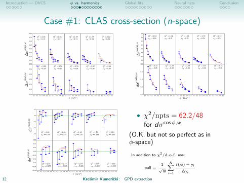
• χ2/npts = 62.2/48for dσcosφ,w
(O.K. but not so perfect as inφ-space)
In addition to χ2/d.o.f. use:
pull ≡1√N
N∑i=1
f (xi )− yi
∆yi
12 Kresimir Kumericki : GPD extraction
Introduction — DVCS φ vs. harmonics Global fits Neural nets Conclusion
Case #1: CLAS cross-section (n-space)
0.00
0.05
0.10
0.15
0.20
0.25
0.30
0.35
0.40
∆σ
sinφ,w
Q2 =1.63xB =0.18
Q2 =1.64xB =0.21
Q2 =1.88xB =0.21
Q2 =1.79xB =0.24
Q2 =2.12xB =0.24
0.1 0.2 0.3 0.4 0.50.00
0.01
0.02
0.03
0.04
0.05
0.06
∆σ
sinφ,w
Q2 =2.35xB =0.28
0.1 0.2 0.3 0.4 0.5
Q2 =2.58xB =0.30
0.1 0.2 0.3 0.4 0.5
−t [GeV2 ]
Q2 =2.78xB =0.34
0.1 0.2 0.3 0.4 0.5
Q2 =2.97xB =0.36
0.1 0.2 0.3 0.4 0.5
Q2 =3.18xB =0.40
0.0
0.2
0.4
0.6
0.8
1.0
1.2
1.4
1.6
dσ
cos0φ,w
Q2 =1.63xB =0.18
Q2 =1.64xB =0.21
Q2 =1.88xB =0.21
Q2 =1.79xB =0.24
Q2 =2.12xB =0.24
0.1 0.2 0.3 0.4 0.50.00
0.05
0.10
0.15
0.20
dσ
cos0φ,w
Q2 =2.35xB =0.28
0.1 0.2 0.3 0.4 0.5
Q2 =2.58xB =0.30
0.1 0.2 0.3 0.4 0.5
−t [GeV2 ]
Q2 =2.78xB =0.34
0.1 0.2 0.3 0.4 0.5
Q2 =2.97xB =0.36
0.1 0.2 0.3 0.4 0.5
Q2 =3.18xB =0.40
0.4
0.3
0.2
0.1
0.0
0.1
dσ
cosφ,w
Q2 =1.63xB =0.185
Q2 =1.64xB =0.214
Q2 =1.88xB =0.215
Q2 =1.79xB =0.244
Q2 =2.12xB =0.245
0.1 0.2 0.3 0.4 0.50.05
0.04
0.03
0.02
0.01
0.00
0.01
0.02
0.03
dσ
cosφ,w
Q2 =2.35xB =0.275
0.1 0.2 0.3 0.4 0.5
Q2 =2.58xB =0.305
0.1 0.2 0.3 0.4 0.5
−t [GeV2 ]
Q2 =2.78xB =0.335
0.1 0.2 0.3 0.4 0.5
Q2 =2.97xB =0.365
0.1 0.2 0.3 0.4 0.5
Q2 =3.18xB =0.400
• χ2/npts = 62.2/48for dσcosφ,w
(O.K. but not so perfect as inφ-space)
In addition to χ2/d.o.f. use:
pull ≡1√N
N∑i=1
f (xi )− yi
∆yi
12 Kresimir Kumericki : GPD extraction
Introduction — DVCS φ vs. harmonics Global fits Neural nets Conclusion
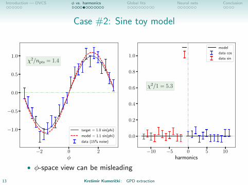
Case #2: Sine toy model
−2 0 2φ
−1.0
−0.5
0.0
0.5
1.0χ2/npts = 1.4
target = 1.0 sin(phi)
model = 1.1 sin(phi)
data (15% noise)
−10 −5 0 5 10harmonics
0.0
0.2
0.4
0.6
0.8
1.0
χ2/1 = 5.3
model
data cos
data sin
• φ-space view can be misleading
13 Kresimir Kumericki : GPD extraction
Introduction — DVCS φ vs. harmonics Global fits Neural nets Conclusion
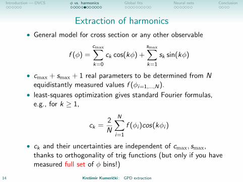
Extraction of harmonics
• General model for cross section or any other observable
f (φ) =cmax∑k=0
ck cos(kφ) +smax∑k=1
sk sin(kφ)
• cmax + smax + 1 real parameters to be determined from Nequidistantly measured values f (φi=1,...,N).
• least-squares optimization gives standard Fourier formulas,e.g., for k ≥ 1,
ck =2
N
N∑i=1
f (φi )cos(kφi )
• ck and their uncertainties are independent of cmax, smax,thanks to orthogonality of trig functions (but only if you havemeasured full set of φ bins!)
14 Kresimir Kumericki : GPD extraction
Introduction — DVCS φ vs. harmonics Global fits Neural nets Conclusion
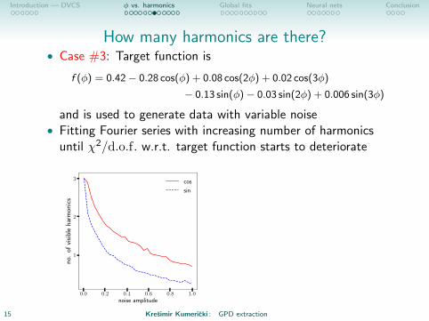
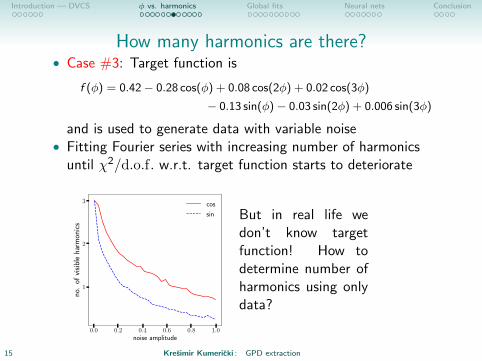
How many harmonics are there?• Case #3: Target function is
f (φ) = 0.42− 0.28 cos(φ) + 0.08 cos(2φ) + 0.02 cos(3φ)
− 0.13 sin(φ)− 0.03 sin(2φ) + 0.006 sin(3φ)
and is used to generate data with variable noise• Fitting Fourier series with increasing number of harmonics
until χ2/d.o.f. w.r.t. target function starts to deteriorate
0.0 0.2 0.4 0.6 0.8 1.0noise amplitude
1
2
3
no.
ofvi
sibl
eha
rmon
ics
cos
sin
But in real life wedon’t know targetfunction! How todetermine number ofharmonics using onlydata?
15 Kresimir Kumericki : GPD extraction
Introduction — DVCS φ vs. harmonics Global fits Neural nets Conclusion
How many harmonics are there?• Case #3: Target function is
f (φ) = 0.42− 0.28 cos(φ) + 0.08 cos(2φ) + 0.02 cos(3φ)
− 0.13 sin(φ)− 0.03 sin(2φ) + 0.006 sin(3φ)
and is used to generate data with variable noise• Fitting Fourier series with increasing number of harmonics
until χ2/d.o.f. w.r.t. target function starts to deteriorate
0.0 0.2 0.4 0.6 0.8 1.0noise amplitude
1
2
3
no.
ofvi
sibl
eha
rmon
ics
cos
sin But in real life wedon’t know targetfunction! How todetermine number ofharmonics using onlydata?
15 Kresimir Kumericki : GPD extraction
Introduction — DVCS φ vs. harmonics Global fits Neural nets Conclusion
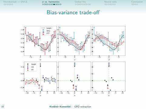
Bias-variance trade-off
−2 0 2φ
0.0
0.2
0.4
0.6
0.8
1.0target
data
FT2
−2 0 2φ
−2 0 2φ
−10 −5 0 5 10n
−0.2
0.0
0.2
0.4
target
cos
sin
−10 −5 0 5 10n
−10 −5 0 5 10n
16 Kresimir Kumericki : GPD extraction
Introduction — DVCS φ vs. harmonics Global fits Neural nets Conclusion
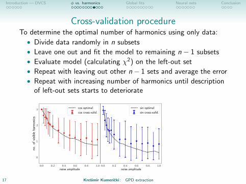
Cross-validation procedureTo determine the optimal number of harmonics using only data:
• Divide data randomly in n subsets
• Leave one out and fit the model to remaining n − 1 subsets
• Evaluate model (calculating χ2) on the left-out set
• Repeat with leaving out other n− 1 sets and average the error
• Repeat with increasing number of harmonics until descriptionof left-out sets starts to deteriorate
0.0 0.2 0.4 0.6 0.8 1.0noise amplitude
0
1
2
3
no.
ofvi
sibl
eha
rmon
ics
cos optimal
cos cross-valid.
0.0 0.2 0.4 0.6 0.8 1.0noise amplitude
sin optimal
sin cross-valid.
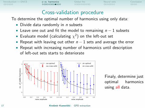
Finaly, determine justoptimal harmonicsusing all data.
17 Kresimir Kumericki : GPD extraction
Introduction — DVCS φ vs. harmonics Global fits Neural nets Conclusion
Cross-validation procedureTo determine the optimal number of harmonics using only data:
• Divide data randomly in n subsets
• Leave one out and fit the model to remaining n − 1 subsets
• Evaluate model (calculating χ2) on the left-out set
• Repeat with leaving out other n− 1 sets and average the error
• Repeat with increasing number of harmonics until descriptionof left-out sets starts to deteriorate
0.0 0.2 0.4 0.6 0.8 1.0noise amplitude
0
1
2
3
no.
ofvi
sibl
eha
rmon
ics
cos optimal
cos cross-valid.
0.0 0.2 0.4 0.6 0.8 1.0noise amplitude
sin optimal
sin cross-valid.
Finaly, determine justoptimal harmonicsusing all data.
17 Kresimir Kumericki : GPD extraction
Introduction — DVCS φ vs. harmonics Global fits Neural nets Conclusion
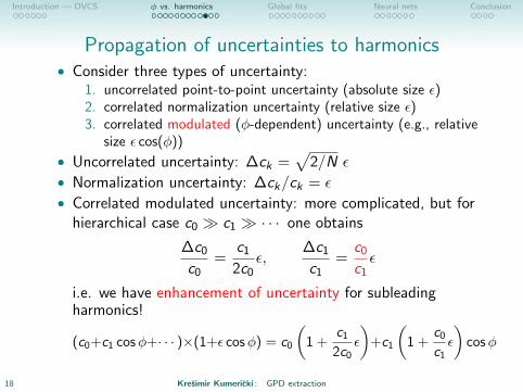
Propagation of uncertainties to harmonics• Consider three types of uncertainty:
1. uncorrelated point-to-point uncertainty (absolute size ε)2. correlated normalization uncertainty (relative size ε)3. correlated modulated (φ-dependent) uncertainty (e.g., relative
size ε cos(φ))
• Uncorrelated uncertainty: ∆ck =√
2/N ε
• Normalization uncertainty: ∆ck/ck = ε
• Correlated modulated uncertainty: more complicated, but forhierarchical case c0 � c1 � · · · one obtains
∆c0
c0=
c1
2c0ε,
∆c1
c1=
c0
c1ε
i.e. we have enhancement of uncertainty for subleadingharmonics!
(c0+c1 cosφ+· · · )×(1+ε cosφ) = c0
(1 +
c1
2c0ε
)+c1
(1 +
c0
c1ε
)cosφ
18 Kresimir Kumericki : GPD extraction
Introduction — DVCS φ vs. harmonics Global fits Neural nets Conclusion
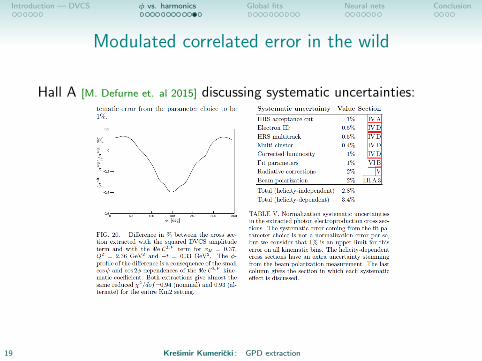
Modulated correlated error in the wild
Hall A [M. Defurne et. al 2015] discussing systematic uncertainties:
19 Kresimir Kumericki : GPD extraction
Introduction — DVCS φ vs. harmonics Global fits Neural nets Conclusion
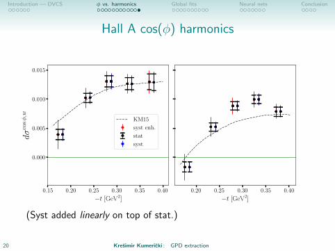
Hall A cos(φ) harmonics
0.15 0.20 0.25 0.30 0.35 0.40
−t [GeV2]
0.000
0.005
0.010
0.015
dσ
cosφ,w
KM15
syst enh.
stat
syst
0.20 0.25 0.30 0.35 0.40
−t [GeV2]
(Syst added linearly on top of stat.)
20 Kresimir Kumericki : GPD extraction
Introduction — DVCS φ vs. harmonics Global fits Neural nets Conclusion
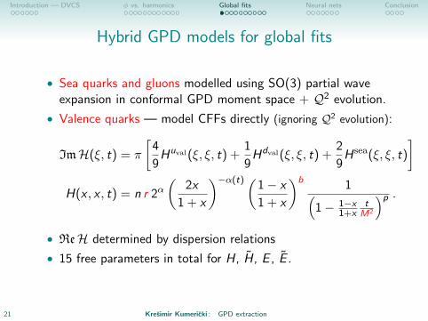
Hybrid GPD models for global fits
• Sea quarks and gluons modelled using SO(3) partial waveexpansion in conformal GPD moment space + Q2 evolution.
• Valence quarks — model CFFs directly (ignoring Q2 evolution):
ImH(ξ, t) = π
[4
9Huval(ξ, ξ, t) +
1
9Hdval(ξ, ξ, t) +
2
9Hsea(ξ, ξ, t)
]H(x , x , t) = n r 2α
(2x
1 + x
)−α(t)(1− x
1 + x
)b 1(1− 1−x
1+xt
M2
)p .• ReH determined by dispersion relations
• 15 free parameters in total for H, H, E , E .
21 Kresimir Kumericki : GPD extraction
Introduction — DVCS φ vs. harmonics Global fits Neural nets Conclusion
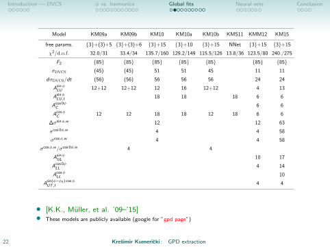
Model KM09a KM09b KM10 KM10a KM10b KMS11 KMM12 KM15
free params. {3}+(3)+5 {3}+(3)+6 {3}+15 {3}+10 {3}+15 NNet {3}+15 {3}+15
χ2/d.o.f. 32.0/31 33.4/34 135.7/160 129.2/149 115.5/126 13.8/36 123.5/80 240./275
F2 {85} {85} {85} {85} {85} {85} {85}σDVCS (45) (45) 51 51 45 11 11
dσDVCS/dt (56) (56) 56 56 56 24 24
AsinφLU 12+12 12+12 12 16 12+12 4 13
AsinφLU,I 18 18 18 6 6
Acos 0φC 6 6
AcosφC 12 12 18 18 12 18 6 6
∆σsinφ,w 12 12 63
σcos 0φ,w 4 4 58
σcosφ,w 4 4 58
σcosφ,w/σcos 0φ,w 4 4
AsinφUL 10 17
Acos 0φLL 4 14
AcosφLL 10
Asin(φ−φS ) cosφUT ,I 4 4
• [K.K., Muller, et al. ’09–’15]• These models are publicly available (google for ”gpd page”)
22 Kresimir Kumericki : GPD extraction
Introduction — DVCS φ vs. harmonics Global fits Neural nets Conclusion
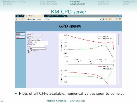
KM GPD server
• Plots of all CFFs available; numerical values soon to come . . .
23 Kresimir Kumericki : GPD extraction
Introduction — DVCS φ vs. harmonics Global fits Neural nets Conclusion
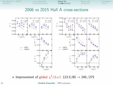
2006 vs 2015 Hall A cross-sections
0.2 0.3 0.4
−t [GeV2]
0.000
0.005
0.010
0.015
0.020
∆σsinφ,w
Q 2 = 1. 50xB = 0. 36
0.2 0.3 0.4
−t [GeV2]
Q 2 = 1. 90xB = 0. 36
0.2 0.3 0.4
Q 2 = 2. 30xB = 0. 36
0.2 0.3 0.40.00
0.03
0.06
dσcos0φ,w
0.2 0.3 0.4
−t [GeV2]
0.00
0.01
dσcosφ,w
KM15
KMM12
0.2 0.3 0.4
−t [GeV2]
0.000
0.005
0.010
0.015
0.020
∆σsinφ,w
Q 2 = 1. 57xB = 0. 38
0.2 0.3 0.4
Q 2 = 1. 94xB = 0. 37
0.2 0.3 0.4
Q 2 = 2. 32xB = 0. 36
0.2 0.3 0.40.00
0.03
0.06
dσcos0φ,w
0.2 0.3 0.4
0.2 0.3 0.4
−t [GeV2]
0.00
0.01
dσcosφ,w
KM15
KMM12
0.2 0.3 0.4
−t [GeV2]
• Improvement of global χ2/d.o.f. 123.5/80 → 240./275
24 Kresimir Kumericki : GPD extraction
Introduction — DVCS φ vs. harmonics Global fits Neural nets Conclusion
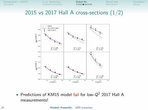
2015 vs 2017 Hall A cross-sections (1/2)
0.2 0.3 0.40.00
0.02
0.04
0.06
0.08
dco
s0,w
Q2 = 1.98E = 5.55
KM15only 2017 dataHall A 2017
0.2 0.3 0.4
Q2 = 1.74E = 5.55
0.2 0.3 0.4
Q2 = 1.51E = 5.55
0.2 0.3 0.4t [GeV2]
0.00
0.05
0.10
0.15
0.20
dco
s0,w
Q2 = 1.99E = 4.46
0.2 0.3 0.4t [GeV2]
Q2 = 1.74E = 4.46
0.2 0.3 0.4t [GeV2]
Q2 = 1.50E = 3.35
• Predictions of KM15 model fail for low-Q2 2017 Hall Ameasurements!
25 Kresimir Kumericki : GPD extraction
Introduction — DVCS φ vs. harmonics Global fits Neural nets Conclusion
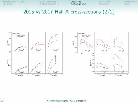
2015 vs 2017 Hall A cross-sections (2/2)
0.2 0.3 0.4
0.00
0.02
0.04
0.06
dco
s,w
Q2 = 1.98E = 5.55
KM15only 2017 dataHall A 2017
0.2 0.3 0.4
Q2 = 1.74E = 5.55
0.2 0.3 0.4
Q2 = 1.51E = 5.55
0.2 0.3 0.4t [GeV2]
0.00
0.02
0.04
0.06
dco
s,w
Q2 = 1.99E = 4.46
0.2 0.3 0.4t [GeV2]
Q2 = 1.74E = 4.46
0.2 0.3 0.4t [GeV2]
Q2 = 1.50E = 3.35
0.2 0.3 0.40.000
0.005
0.010
0.015
sin,w
Q2 = 1.98E = 5.55
KM15only 2017 dataHall A 2017
0.2 0.3 0.4
Q2 = 1.74E = 5.55
0.2 0.3 0.4
Q2 = 1.51E = 5.55
0.2 0.3 0.4t [GeV2]
0.00
0.01
0.02
0.03
0.04
sin,w
Q2 = 1.74E = 4.46
0.2 0.3 0.4t [GeV2]
Q2 = 1.50E = 3.35
26 Kresimir Kumericki : GPD extraction
Introduction — DVCS φ vs. harmonics Global fits Neural nets Conclusion
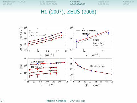
H1 (2007), ZEUS (2008)
27 Kresimir Kumericki : GPD extraction
Introduction — DVCS φ vs. harmonics Global fits Neural nets Conclusion
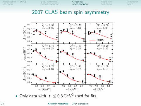
2007 CLAS beam spin asymmetry
0.0
0.1
0.2
0.3
0.4ALU(9
0◦) Q 2 = 2. 30
xB = 0. 35Q 2 = 2. 70xB = 0. 36
Q 2 = 3. 00xB = 0. 36
KM15
0.0
0.1
0.2
0.3
0.4
ALU(9
0◦) Q 2 = 1. 70
xB = 0. 25Q 2 = 1. 90xB = 0. 25
Q 2 = 2. 20xB = 0. 25
0.3 0.6 0.9 1.2
−t [GeV2]
0.0
0.1
0.2
0.3
0.4
ALU(9
0◦) Q 2 = 1. 20
xB = 0. 13
0.3 0.6 0.9 1.2
−t [GeV2]
Q 2 = 1. 40xB = 0. 17
0.3 0.6 0.9 1.2
−t [GeV2]
Q 2 = 1. 60xB = 0. 18
• Only data with |t| ≤ 0.3GeV2 used for fits.
28 Kresimir Kumericki : GPD extraction
Introduction — DVCS φ vs. harmonics Global fits Neural nets Conclusion
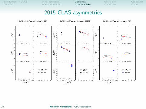
2015 CLAS asymmetries
29 Kresimir Kumericki : GPD extraction
Introduction — DVCS φ vs. harmonics Global fits Neural nets Conclusion
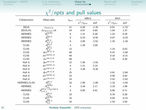
χ2/npts and pull valuesCollaboration Observable npts
KMM12 KM15
χ2/npts pull χ2/npts pull
ZEUS σDVCS 11 0.49 -1.76 0.51 -1.74
ZEUS,H1 dσDVCS/dt 24 0.97 0.85 1.04 1.37
HERMES Acos 0φC 6 1.31 0.49 1.24 0.29
HERMES AcosφC 6 0.24 -0.56 0.07 -0.20
HERMES AsinφLU,I 6 2.08 -2.52 1.34 -1.28
CLAS AsinφLU 4 1.28 2.09
CLAS AsinφLU 13 1.24 0.63
CLAS ∆σsinφ,w 48 0.41 -1.66
CLAS dσcos 0φ,w 48 0.16 -0.21
CLAS dσcosφ,w 48 1.16 6.36
Hall A ∆σsinφ,w 12 1.06 -2.55
Hall A dσcos 0φ,w 4 1.21 2.14
Hall A dσcosφ,w 4 3.49 -0.26
Hall A ∆σsinφ,w 15 0.81 -2.84
Hall A dσcos 0φ,w 10 0.40 0.92
Hall A dσcosφ,w 10 2.52 -2.42
HERMES,CLAS AsinφUL 10 1.90 -1.89 1.10 -1.94
HERMES Acos 0φLL 4 3.44 2.17 3.19 1.99
HERMES Asin(φ−φS ) cosφUT,I 4 0.90 0.61 0.90 0.71
CLAS AsinφUL 10 0.76 0.38
CLAS Acos 0φLL 10 0.50 -0.22
CLAS AcosφLL 10 1.54 2.40
30 Kresimir Kumericki : GPD extraction
Introduction — DVCS φ vs. harmonics Global fits Neural nets Conclusion
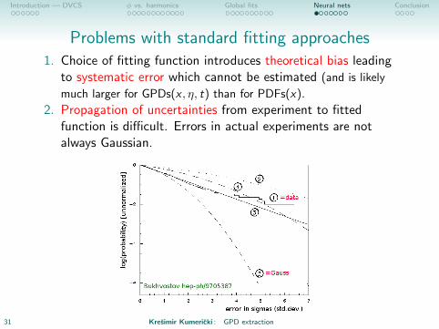
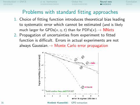
Problems with standard fitting approaches1. Choice of fitting function introduces theoretical bias leading
to systematic error which cannot be estimated (and is likely
much larger for GPDs(x , η, t) than for PDFs(x).
→ NNets
2. Propagation of uncertainties from experiment to fittedfunction is difficult. Errors in actual experiments are notalways Gaussian.
→ Monte Carlo error propagation
31 Kresimir Kumericki : GPD extraction
Introduction — DVCS φ vs. harmonics Global fits Neural nets Conclusion
Problems with standard fitting approaches1. Choice of fitting function introduces theoretical bias leading
to systematic error which cannot be estimated (and is likely
much larger for GPDs(x , η, t) than for PDFs(x).→ NNets2. Propagation of uncertainties from experiment to fitted
function is difficult. Errors in actual experiments are notalways Gaussian.→ Monte Carlo error propagation
31 Kresimir Kumericki : GPD extraction
Introduction — DVCS φ vs. harmonics Global fits Neural nets Conclusion
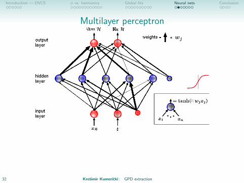
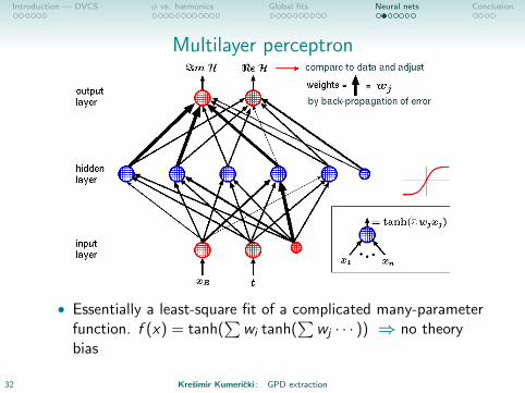
Multilayer perceptron
• Essentially a least-square fit of a complicated many-parameterfunction. f (x) = tanh(
∑wi tanh(
∑wj · · · )) ⇒ no theory
bias
32 Kresimir Kumericki : GPD extraction
Introduction — DVCS φ vs. harmonics Global fits Neural nets Conclusion
Multilayer perceptron
• Essentially a least-square fit of a complicated many-parameterfunction. f (x) = tanh(
∑wi tanh(
∑wj · · · )) ⇒ no theory
bias
32 Kresimir Kumericki : GPD extraction
Introduction — DVCS φ vs. harmonics Global fits Neural nets Conclusion
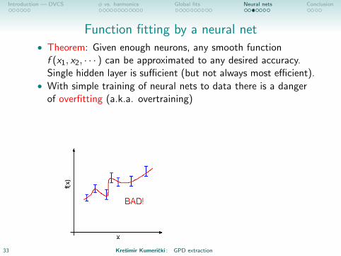
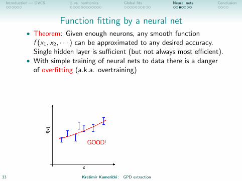
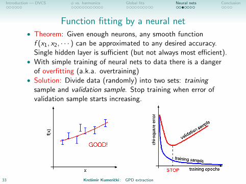
Function fitting by a neural net• Theorem: Given enough neurons, any smooth functionf (x1, x2, · · · ) can be approximated to any desired accuracy.Single hidden layer is sufficient (but not always most efficient).
• With simple training of neural nets to data there is a dangerof overfitting (a.k.a. overtraining)
• Solution: Divide data (randomly) into two sets: trainingsample and validation sample. Stop training when error ofvalidation sample starts increasing.
33 Kresimir Kumericki : GPD extraction
Introduction — DVCS φ vs. harmonics Global fits Neural nets Conclusion
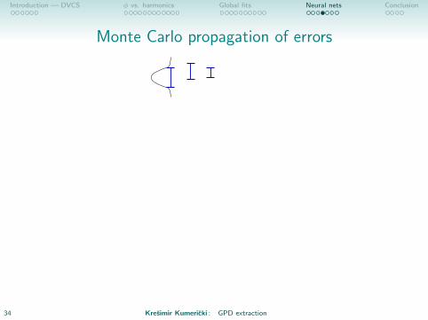
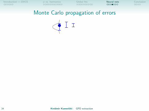
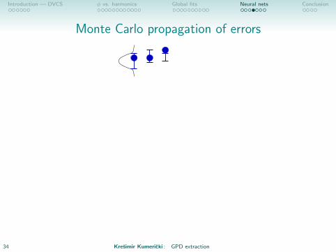
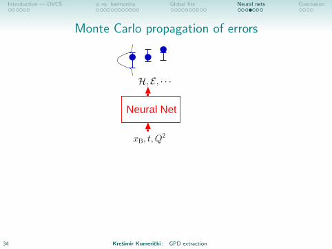
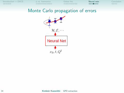
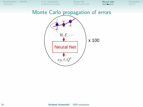
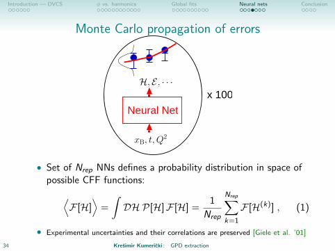
Monte Carlo propagation of errors
H, E , · · ·
Neural Net
xB, t, Q2
x 100
H, E , · · ·
Neural Net
xB, t, Q2
x 100
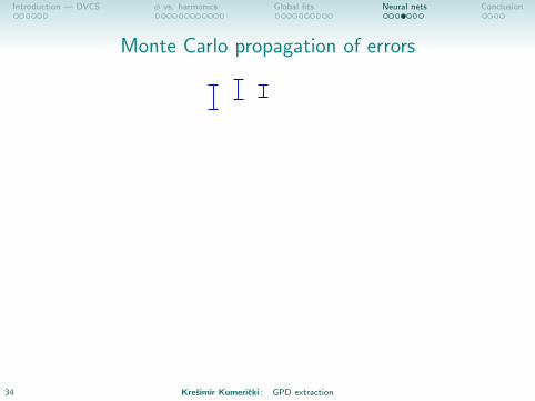
• Set of Nrep NNs defines a probability distribution in space ofpossible CFF functions:⟨
F [H]⟩
=
∫DH P[H]F [H] =
1
Nrep
Nrep∑k=1
F [H(k)] , (1)
• Experimental uncertainties and their correlations are preserved [Giele et al. ’01]
34 Kresimir Kumericki : GPD extraction
Introduction — DVCS φ vs. harmonics Global fits Neural nets Conclusion
Monte Carlo propagation of errors
H, E , · · ·
Neural Net
xB, t, Q2
x 100
H, E , · · ·
Neural Net
xB, t, Q2
x 100
• Set of Nrep NNs defines a probability distribution in space ofpossible CFF functions:⟨
F [H]⟩
=
∫DH P[H]F [H] =
1
Nrep
Nrep∑k=1
F [H(k)] , (1)
• Experimental uncertainties and their correlations are preserved [Giele et al. ’01]
34 Kresimir Kumericki : GPD extraction
Introduction — DVCS φ vs. harmonics Global fits Neural nets Conclusion
Monte Carlo propagation of errors
H, E , · · ·
Neural Net
xB, t, Q2
x 100
• Set of Nrep NNs defines a probability distribution in space ofpossible CFF functions:⟨
F [H]⟩
=
∫DH P[H]F [H] =
1
Nrep
Nrep∑k=1
F [H(k)] , (1)
• Experimental uncertainties and their correlations are preserved [Giele et al. ’01]
34 Kresimir Kumericki : GPD extraction
Introduction — DVCS φ vs. harmonics Global fits Neural nets Conclusion
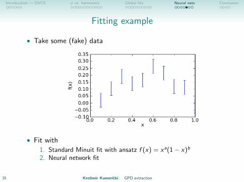
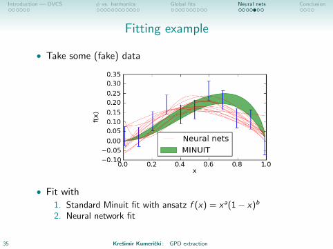
Fitting example
• Take some (fake) data
• Fit with
1. Standard Minuit fit with ansatz f (x) = xa(1− x)b
2. Neural network fit
35 Kresimir Kumericki : GPD extraction
Introduction — DVCS φ vs. harmonics Global fits Neural nets Conclusion
Fitting example
• Take some (fake) data
• Fit with
1. Standard Minuit fit with ansatz f (x) = xa(1− x)b
2. Neural network fit
35 Kresimir Kumericki : GPD extraction
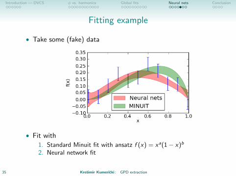
Introduction — DVCS φ vs. harmonics Global fits Neural nets Conclusion
Fitting example
• Take some (fake) data
• Fit with
1. Standard Minuit fit with ansatz f (x) = xa(1− x)b
2. Neural network fit
35 Kresimir Kumericki : GPD extraction
Introduction — DVCS φ vs. harmonics Global fits Neural nets Conclusion
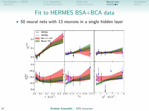
Fit to HERMES BSA+BCA data
• 50 neural nets with 13 neurons in a single hidden layer
36 Kresimir Kumericki : GPD extraction
Introduction — DVCS φ vs. harmonics Global fits Neural nets Conclusion
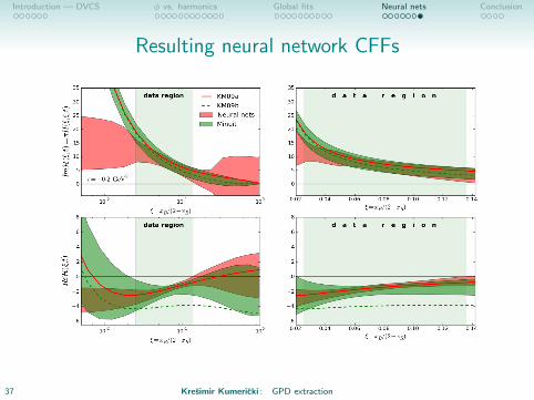
Resulting neural network CFFs
37 Kresimir Kumericki : GPD extraction
Introduction — DVCS φ vs. harmonics Global fits Neural nets Conclusion
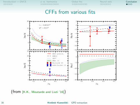
CFFs from various fits
0
5
10
15
20
ImH
t = −0.28 GeV2
Q2 ∼ 2 GeV2
−12
−10
−8
−6
−4
−2
0
2
ReH
0.1 0.2 0.3 0.4
xB
0
2
4
6
8
10
12
ImH
KM15 prelim.
KMM12
GK07
NNet 14
Moutarde 09
Boer/Guidal 14
0.1 0.2 0.3 0.4
xB
−20
−15
−10
−5
0
5
ReE
(from [K.K., Moutarde and Liuti ’16])
38 Kresimir Kumericki : GPD extraction
Introduction — DVCS φ vs. harmonics Global fits Neural nets Conclusion
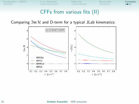
CFFs from various fits (II)
Comparing ImH and D-term for a typical JLab kinematics:
• We need access to ERBL region.
39 Kresimir Kumericki : GPD extraction
Introduction — DVCS φ vs. harmonics Global fits Neural nets Conclusion
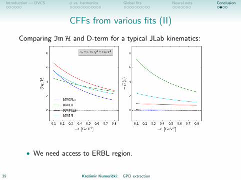
CFFs from various fits (II)
Comparing ImH and D-term for a typical JLab kinematics:
• We need access to ERBL region.
39 Kresimir Kumericki : GPD extraction
Introduction — DVCS φ vs. harmonics Global fits Neural nets Conclusion
Going beyond first approximations
Published DVCS data (apart from new 2017 Hall A) is welldescribed within leading order, leading twist and otherapproximations. Some available corrections:
• NLO evolution and NLO coefficient functions
• finite-t and target mass corrections [Braun et al. ’14]
• twist-3 GPDs
• massive charm [Noritzsch ’03]
• small-x resummation
can maybe be absorbed in redefinition of GPDs (think ”DVCSscheme” factorization), but have to be taken into account whenworking with more processes (striving towards universal GPDs) andwith more precise future data.
40 Kresimir Kumericki : GPD extraction
Introduction — DVCS φ vs. harmonics Global fits Neural nets Conclusion
Summary
• Global fits of all proton DVCS data using flexible hybridmodels were in healthy shape until 2017 (some tension forfirst cos(φ) harmonic of JLab cross sections).
• New Hall A 2017 data present a challenge
• Standard global model fitting and neural networks approachare complementing each other
The End
41 Kresimir Kumericki : GPD extraction