1

Terrestrial Observation and Prediction System (TOPS): Developing ecological nowcasts and forecasts by integrating surface, satellite and climate data with simulation models.

Ramakrishna Nemani1, Petr Votava2, Andrew Michaelis2, Michael White3, Forrest

Melton2, Cristina Milesi2, Lars Pierce2 , Keith Golden4, Hirofumi Hashimoto2, Kazuhito

Ichii5, Lee Johnson2, Matt Jolly6, Ranga Myneni7, Christina Tague8, Joseph Coughlan1,

and Steve Running9.

1NASA Ames Research Center, Moffett Field, CA 2California State University, Monterey Bay, Seaside, CA 3Utah State University, Logan, UT 4Google Inc., Mountain View, CA 5San Jose State University, San Jose, CA 6U.S. Forest Service, Missoula, MT 7Boston University, Boston, MA 8San Diego State University, San Diego, CA 9University of Montana, Missoula, MT

Abstract

Ecological Forecasting, predicting the effects of changes in the physical, chemical, and

biological environments on ecosystem state and activity, is an emerging field with

significant socio-economic implications. Though the concepts behind and expectations

for ecological forecasting are clear, progress towards producing consistent, reliable,

and objective forecasts has been slow. Lack of infrastructure for integrating a variety

of modeling tools, information technologies, and ground and satellite data sets that

could serve the diverse needs of eco-hydrological community has been one key

impediment. Here, we describe our efforts at such an integrated system called the

2

Terrestrial Observation and Prediction System (TOPS). TOPS is a data and modeling

software system designed to seamlessly integrate data from satellite, aircraft, and

ground sensors with weather/climate and application models to expeditiously produce

operational nowcasts and forecasts of ecological conditions. TOPS has been operating

at a variety of spatial scales, ranging from individual vineyard blocks in California,

and predicting weekly irrigation requirements, to global scale producing regular

monthly assessments of global vegetation net primary production.

Introduction

The latest generation of NASA Earth Observing System (EOS) satellites has

brought a new dimension to monitoring the living part of the Earth system – the

biosphere. EOS data can now measure weekly global productivity of plants and ocean

chlorophyll and related biophysical factors, such as changes to land cover and to the rate

of snowmelt. However, a greater economic benefit would be realized by forecasting

biospheric conditions (Clark et al., 2001). Such predictive ability would provide an

advanced decision-making tool to be used in the mitigation of natural hazards or in the

exploitation of economically advantageous trends. Imagine if it were possible to

accurately predict shortfalls or bumper crops, epidemics of vector-borne diseases such as

malaria and West Nile virus, or wildfire danger as much as 3 to 6 months in advance.

Such a predictive tool would allow improved preparation and logistical efficiencies.

Forecasting provides decision-makers with insight into the future status of

ecosystems and allows for the evaluation of the status quo as well as alternatives or

preparatory actions that could be taken in anticipation of future conditions. Whether

preparing for the summer fire season or for spring floods, knowledge of the magnitude

and direction of future conditions can save time, money, and valuable resources. Space-

and ground-based observations have significantly improved the ability to monitor natural

resources and to identify potential changes, but these observations can describe current

conditions only. This information is useful, but many resource managers often need to

make decisions months in advance for the coming season. Recent advances in climate

3

forecasting have elicited strong interest in a variety of economic sectors: agriculture

(Cane et al., 1994), health (Thomson et al., 2005) and water resources (Wood et al.,

2001). The climate forecasting capabilities of coupled ocean-atmosphere global

circulation models (GCMs) have steadily improved over the past decade (Zebiak 2003).

Given observed anomalies in sea-surface temperatures (SSTs) from satellite data, GCMs

are now able to forecast general climatic conditions, including temperature and

precipitation trends, 6 to 12 months into the future with reasonable accuracy (Goddard et

al., 2001; Robertson et al., 2004).

While such climatic forecasts alone are useful, the advances in ecosystem

modeling allow specific exploration of the direct impacts of these future climate trends

on the ecosystem. One day predictions made in March might accurately forecast whether

Montana’s July winter wheat harvest will be greater or less than normal, and whether the

growing season will be early or late.

One of the key problems in adapting climate forecasts to natural ecosystems is the

"memory" that these systems carry from one season to the next. For example, soil

moisture levels, plant seed banks, and fire fuel build-up are all affected by cumulative

ecosystem processes that occur over many seasons or years. Simulation models are often

the best tools to carry forward information about this spatio-temporal memory. The

ability of models to describe and to predict ecosystem behavior has advanced

dramatically over the last two decades, driven by major improvements in process-level

understanding, climate mapping, computing technology, and the availability of a wide

range of satellite- and ground-based sensors (Waring and Running 1998). In this chapter,

we summarize the efforts of the Ecological Forecasting Group at NASA Ames Research

Center over the past six years to integrate advances in these areas and develop an

operational ecological forecasting system.

Background of Ecological Forecasting

Ecological Forecasting (EF) predicts the effects of changes in the physical,

chemical, and biological environments on ecosystem state and activity (Clark et al.,

4

2001). EF is pursued with a variety of tools and techniques in different communities. For

example, for community ecologists EF commonly includes methods for describing or

predicting the ecological niche for various species. Much of invasive species forecasting

falls in this area, where a set of conditions associated with the presence/absence of a

species is derived and then these empirical relations are used to predict the occurrence or

potential for occurrence of that species within a landscape. Similarly, bio-geographers

use EF to predict species/community compositions in response to changes in long-term

climate or geo-chemical conditions. Climate change and carbon cycling research falls in

this category of predicting the state and/or functioning of ecosystems over long-lead

times of decades to centuries. In contrast, the eco-hydrological community uses EF as a

way of extending weather/climate predictions, with lead times ranging from days to

months, for use in operational decision-making. Examples include forecasts of frost

damage, flood/streamflow, crop yield, and pest/disease outbreaks. Though such forecasts

are age-old among practitioners of various trades, there has been much subjectivity in the

decision-making process that is hard to quantify and pass on to later generations.

Providing an operational forecasting capability brings a new level of complexity to

creating, verifying, and distributing information that is worth acting upon.

Components of ecological forecasting for eco-hydrological applications

Increasing interest in ecological forecasting is evident from several recent

applications ranging from streamflows (Wood et al., 2001), crop yields (Cane et al.,

1994) and human health (Thompson et al., 2006). These attempts tend to focus on

specific watersheds or a geographic location with a very specific application; therefore

they do not deal with EF as a broad theme associated with certain tools and technologies.

Our past heritage in eco-hydrology and NASA’s strengths in global observations and

technology led us to focus on the development of a general data and modeling system

that allows to produce operational nowcasts and forecasts relevant for many in the eco-

hydrological community. Here we briefly review the important components that make

our approach to EF possible, extensible, and economically viable.

5

Ecosystem Models: As in numerical weather prediction, models form the basis for EF.

These models range in complexity, computational requirements, and in the representation

of the spatio-temporal details of a given process or system. For example, biogeochemical

cycling models are often complex and versatile in the sense that the basic ingredients that

they simulate (carbon, water, nutrient cycling) form the core information for a variety of

biospheric activities of economic value. For example, changes in carbon cycling

expressed as net primary production (NPP) can be a key indicator of crop yields, forage

production or production of board feet of wood. These models use the

Soil-Plant-Atmosphere continuum concept to estimate various water (evaporation,

transpiration, stream flows, and soil water), carbon (net photosynthesis, plant growth) and

nutrient flux (uptake and mineralization) processes. They are adapted for all major

biomes exploiting their unique eco-physiological principles such as drought resistance,

cold tolerance, etc. (e.g. BIOME-BGC, Waring and Running 1998; CASA, Potter et al.,

2003). The models are initialized with ground-based soil physical properties and satellite-

based vegetation information (type and density of plants). Following the initialization

process, daily weather conditions (max/min temperatures, solar radiation, humidity, and

rainfall) are used to drive various ecosystem processes (e.g., soil moisture, transpiration,

evaporation, photosynthesis, and snowmelt) that can be translated into drought, crop

yields, NPP, and water yield estimates. We currently use a diagnostic (with satellite data

input) version of BGC to produce nowcasts and a prognostic (without satellite data

inputs) version of BIOME-BGC to produce forecasts of carbon and water related fluxes.

Extensive discussion on types of ecosystem models and their relevant applications can be

found in Waring and Running (1998) and Canham et al., (1997).

Microclimate mapping from surface weather observations: Access to reliable weather

data is a pre-requisite for ecosystem modeling. The availability of weather observations

has been a key obstacle in the development of real-time EF systems. Historically, weather

data was made available on tapes or CDs months after it was collected and corrected for

errors. This time lag precluded real-time simulations, a precursor to developing

forecasting capability. Through the World Wide Web, however, there are now thousands

6

of on-line weather stations providing real-time weather data. These real-time data include

ground-based observations of max/min/dew temperature and wind speed, satellite-based

solar radiation, and spatially continuous rainfall fields produced by weather agencies.

Another important advancement for EF is the ability to grid point observations

onto the landscape at various spatial resolutions, as observations are rarely sufficient to

represent the spatial variability. Models such as PRISM, DAYMET, and SOGS (Daly et

al.1994; Thornton et al. 1997; Jolly et al. 2004) ingest point surface observations, and use

topography and other ancillary information to compute spatially continuous

meteorological fields (temperature, humidity, solar radiation, and rainfall) that can be

directly used in ecosystem modeling.

Weather/Climate Forecasts: There is considerable optimism among the climate

community about our ability to forecast climate into the future (Trenberth 1996). This

optimism stems from several recent advancements in climate modeling, such as

improvements in GCMs that have allowed realistic reproduction of observed global

climate (Roads et al. 1999), adaptation of new forecasting strategies, demonstration of the

links between El Niño/Southern Oscillation (ENSO) and short-term climate, and the

ability to forecast ENSO 12-18 months in advance. Barnett et al. (1994) showed that with

the above improvements, GCMs could be used successfully to predict air temperature,

precipitation, and solar radiation at extended lead times over many parts of the world.

Research as well as operational agencies that currently produce and disseminate climate

forecasts includes the NOAA’s National Center for Environmental Prediction, Columbia

University’s International Research Institute, the Scripps Institute of Oceanography’s

Experimental Climate Prediction Center, and others.

Satellite remote sensing: A number of studies over the past two decades have shown the

utility of satellite data for monitoring vegetation (type, density, and production), extent of

flood damage, wildland fire detection, and monitoring snow and drought conditions.

However, many of the products generated from satellite data have been experimental, and

did not have a wide distribution among natural resource managers. Over the past five

years, through NASA’s EOS program, there have been substantial improvements in the

7

way satellite data is acquired, processed, converted to products, and delivered (Table 1).

For example, weekly maps of leaf area index (LAI, area of leaves per unit ground area)

and vegetation indices, key inputs for many ecosystem models, are being generated and

distributed from the NASA/MODIS sensor. A number of other key land products such as

NPP, fire occurrence, snow cover, and surface temperature are available globally at 1-km

resolution every 8 days (Justice et al 1998; Myneni et al. 2002). Without this near-

realtime observing capacity, systems such as TOPS would never have materialized.

Integrated modeling: Numerous studies over the past two decades addressed the logical

steps for modeling land surface processes over various spatial scales, by integrating

ecosystem models with satellite, climate data, and other ancillary information (Waring

and Running 1998). One such attempt that many of us have been part of was the

development of the Regional Hydro-Ecological Simulation System (RHESSys, Band et

al. 1993; Nemani et al. 1993; Tague and Band 2004). RHESSys has been used in various

studies for estimating soil moisture, stream flows, snow pack, and primary production

(Waring and Running 1998). Much of the work using RHESSys has been retrospective,

using past climate and satellite data, mainly to evaluate various issues related to the

parameterization of key variables, scaling and determining the suitability of RHESSys

outputs for use by resource managers (Waring and Running 1998). While this type of

retrospective analysis is useful for long-term management decisions, only a real-time

analysis can provide data necessary for dynamic decision making such as the assessment

of fire risk. Our work has focused on the development of the Terrestrial Observation and

Prediction System (TOPS) to provide this capability for real-time analysis, which is

essential for forecasting ecological conditions desired by decision makers.

The Terrestrial Observation and Prediction System (TOPS)

TOPS is a data and modeling software system designed to seamlessly integrate

data from satellite, aircraft, and ground sensors with weather/climate models and

application models to expeditiously produce operational nowcasts and forecasts of

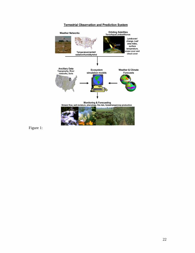
ecological conditions (Figure 1). TOPS provides reliable data on current and predicted

8

ecosystem conditions through automation of the data retrieval, pre-processing,

integration, and modeling steps, allowing TOPS data products to be used in an

operational setting for a range of applications.

Implementation of TOPS over a region consists of first developing the

parameterization scheme for the area of interest. Parameterization inputs include data on

soils, topography, and satellite derived vegetation variables (land cover and LAI).

Observational weather data, gridded from point data or downscaled from previously

gridded data to the appropriate resolution, are then used to run a land surface model, such

as BIOME-BGC (Waring and Running 1998; White et al. 2000). Finally, weather and

climate forecasts are brought into the system as gridded fields and downscaled to the

appropriate resolution to drive the land surface model and generate predictions of future

ecosystem states.

Given the diversity of data sources, formats, and spatio-temporal resolutions,

system automation is critical for the reliable delivery of data products for use in

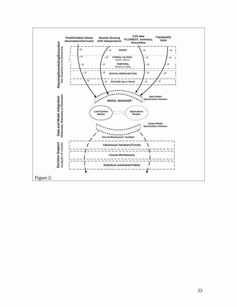
operational decision-making. TOPS has been engineered to automatically ingest various

data fields required for model simulations (Figure 2). Ingested data go through a number

of preprocessing filters in which each parameter is mapped to a list of attributes (e.g.,

source, resolution, and quality). This results in each data field being self-describing to

TOPS component models such that any number of land surface models can be run

without extensive manual interfacing. Similarly, the model outputs also pass through a

specification interface, facilitating post-processing so that model outputs can be presented

as actionable information, as opposed to just another stream of data. TOPS derives its

flexibility and automation capability from two key software components: JDAF (Java

Distributed Application Framework) and the ImageBot planner.

JDAF and IMAGEbot The TOPS software is implemented using a flexible framework that enables fast and easy

integration of new models and data streams into an automated system. The core

components of this framework are JDAF (Java Distributed Application Framework) and

9

IMAGEbot. JDAF consists of a large set of data processing and image analysis algorithms

that are deployed to pre-process and post-process inputs and outputs of the TOPS

ecosystem models. When we want to process new data with our existing models, we re-

use the JDAF algorithms to create intermediate datasets that adhere to the model’s input

specifications so that we can execute our models without having to alter the science

implementation.Because the pre-processing itself can be a very complex process,

involving for example data acquisition, mosaicking, reprojection, subsetting, scaling etc.

We have developed a planner-based agent (IMAGEbot), which automatically generates

the sequence of processing steps needed to perform the appropriate data transformations.

In other words, JDAF provides all the processing components of the system and

IMAGEbot determines how they fit together to achieve the desired goal, creates a plan,

and executes it. This gives a great flexibility to the TOPS software and speeds-up

significantly the integration of both datasets and models into new applications.

Additionally, JDAF provides interface to the database system and to web services

capabilities for seamless access to both data and services provided by TOPS.

As currently deployed within TOPS, JDAF and ImageBot perform two dynamic

functions critical for the real-time monitoring, modeling and forecasting of ecosystem

conditions: gridding of weather observations to create continuous fields of climatic

parameters, and acquisition and processing of satellite data for initializing or verifying

the models.

Climate Gridding

To produce gridded climate fields, the user specifies a geographic area of interest

and the spatial resolution for the gridded fields. The ImageBot planner uses these

specifications to create a data processing plan comprised of a series of requirements and

corresponding actions. For example, ImageBot will identify the acquisition of

topographic data as a requirement, evaluate the possible sources for this data from the

data library, identify the required resolution, and create the set of actions required to

obtain the data at the appropriate resolution. These actions are then passed to JDAF,

10

which fetches the data from the source, and reformats and reprojects the data to meet the

user-specified requirements. Similarly, for meteorological data, ImageBot produces a list

of weather networks available for the region, a list of variables available from each

network, and the frequency of observations available from the network. From this

information and the user-defined set of constraints, ImageBot again formulates a series of

actions specifying which networks and what variables need to be retrieved and input to

the database. After receiving these instructions, JDAF fetches the necessary data, checks

for consistency against historical averages, fills-in missing values from additional

sources, flags missing values, and finally interfaces these observations with the Surface

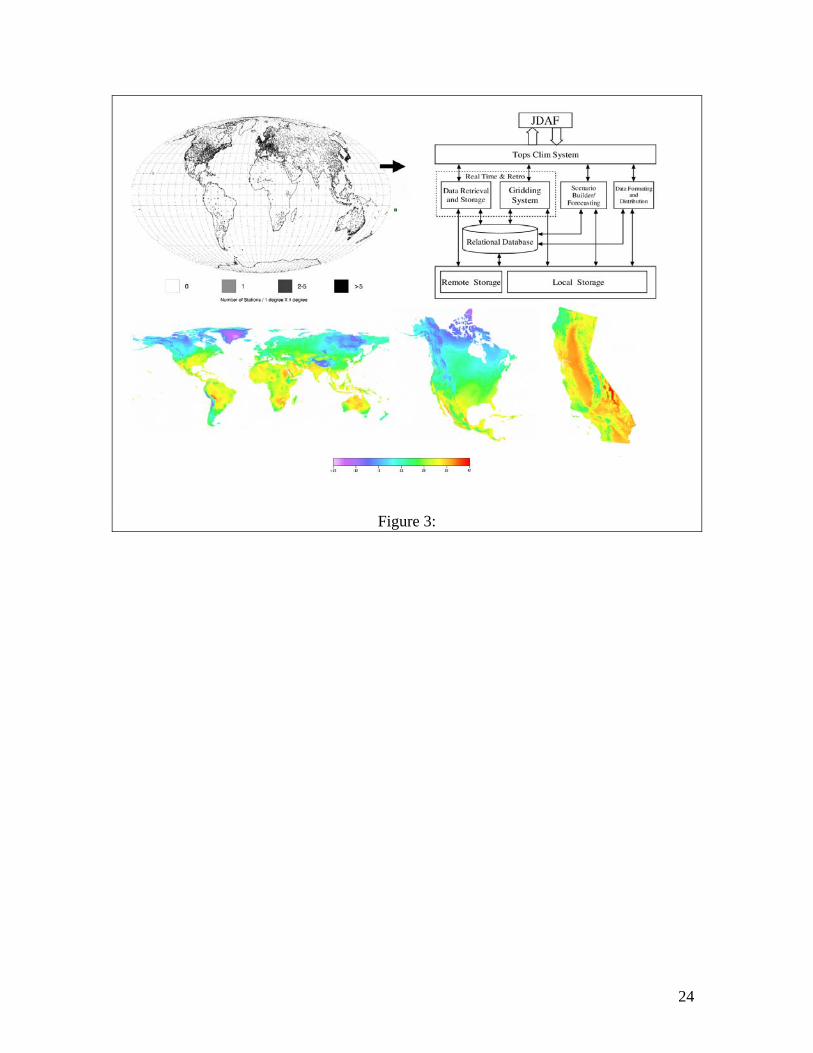
Observation and Gridding System (SOGS, Jolly et al. 2004, Figure 3), a component layer

within TOPS. SOGS is an operational climate-gridding system, and an improvement

upon DAYMET (Thornton et al. 1997), that uses maximum, minimum, and dewpoint

temperatures, in addition to rainfall, to create spatially continuous surfaces for air

temperatures (e.g. Figure 4a), vapor pressure deficits, and incident radiation. The cross-

validation statistics returned from SOGS allow ImageBot to decide if the user-specified

requirements for accuracy have been achieved, or if alternative gridding methods need to

be found.

Acquiring and Processing of Satellite Data

TOPS has access to a number of satellite data sets (Table 1), produced and

processed by either NASA or NOAA. This access involves machine-to-machine, web-

based ordering, and FTP pushes for routine data sets such as those from the NOAA

Geostationary Operational Environmental Satellites (GOES). Similarly to the climate

gridding process described in the previous section, ImageBot defines a set of actions

pertaining to satellite data and products based on user-defined constraints and

requirements. The requirements in this case may include, for example, obtaining LAI and

snow cover data with the following constraints: a minimum resolution of 1km, a weekly

time interval, and a specification to obtain the highest possible quality data available.

From the data library, ImageBot creates a list of sites that provide LAI. ImageBot sends a

11

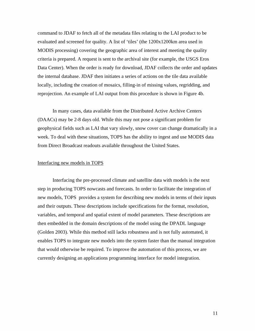
command to JDAF to fetch all of the metadata files relating to the LAI product to be

evaluated and screened for quality. A list of ‘tiles’ (the 1200x1200km area used in

MODIS processing) covering the geographic area of interest and meeting the quality

criteria is prepared. A request is sent to the archival site (for example, the USGS Eros

Data Center). When the order is ready for download, JDAF collects the order and updates

the internal database. JDAF then initiates a series of actions on the tile data available

locally, including the creation of mosaics, filling-in of missing values, regridding, and

reprojection. An example of LAI output from this procedure is shown in Figure 4b.

In many cases, data available from the Distributed Active Archive Centers

(DAACs) may be 2-8 days old. While this may not pose a significant problem for

geophysical fields such as LAI that vary slowly, snow cover can change dramatically in a

week. To deal with these situations, TOPS has the ability to ingest and use MODIS data

from Direct Broadcast readouts available throughout the United States.

Interfacing new models in TOPS

Interfacing the pre-processed climate and satellite data with models is the next

step in producing TOPS nowcasts and forecasts. In order to facilitate the integration of

new models, TOPS provides a system for describing new models in terms of their inputs

and their outputs. These descriptions include specifications for the format, resolution,

variables, and temporal and spatial extent of model parameters. These descriptions are

then embedded in the domain descriptions of the model using the DPADL language

(Golden 2003). While this method still lacks robustness and is not fully automated, it

enables TOPS to integrate new models into the system faster than the manual integration

that would otherwise be required. To improve the automation of this process, we are

currently designing an applications programming interface for model integration.

12

TOPS Nowcasts

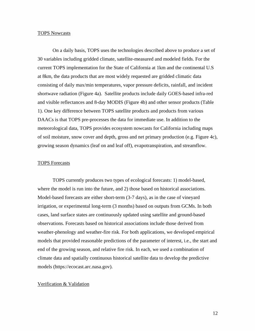
On a daily basis, TOPS uses the technologies described above to produce a set of

30 variables including gridded climate, satellite-measured and modeled fields. For the

current TOPS implementation for the State of California at 1km and the continental U.S

at 8km, the data products that are most widely requested are gridded climatic data

consisting of daily max/min temperatures, vapor pressure deficits, rainfall, and incident

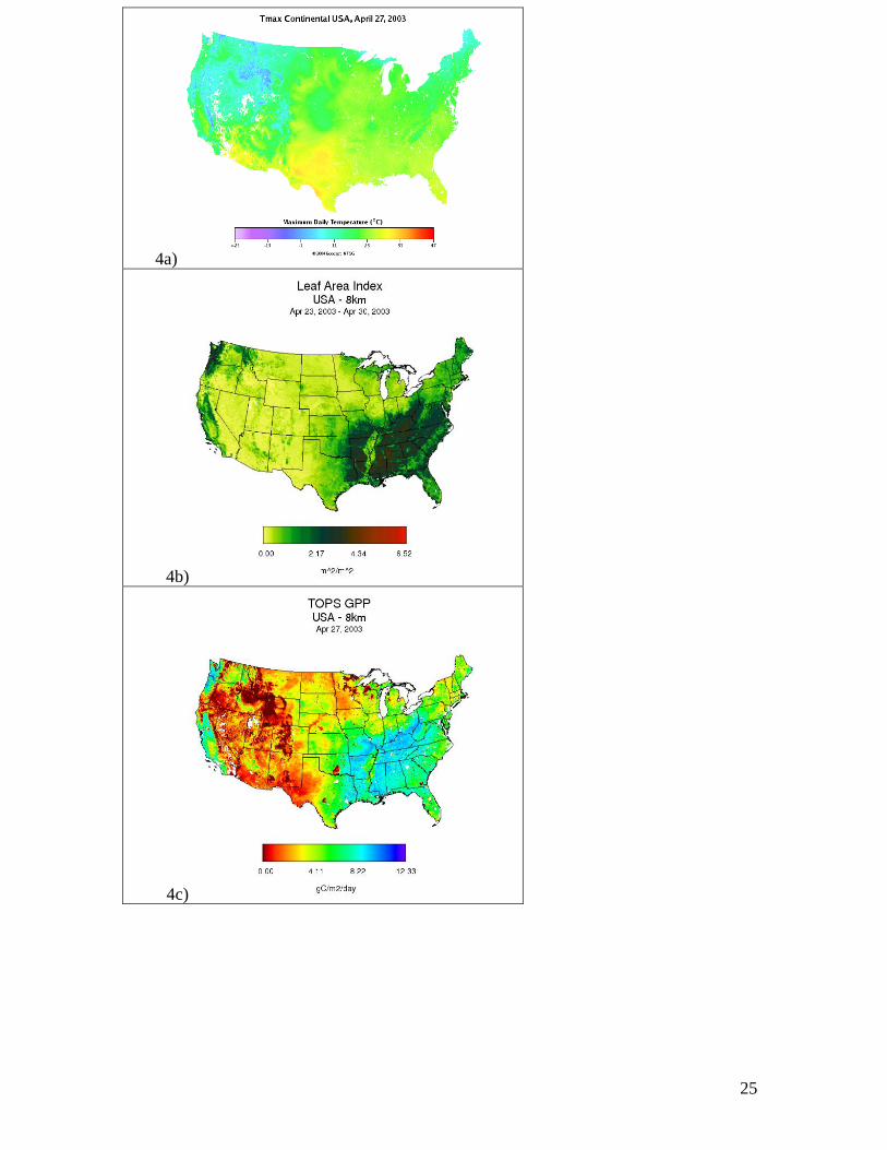
shortwave radiation (Figure 4a). Satellite products include daily GOES-based infra-red

and visible reflectances and 8-day MODIS (Figure 4b) and other sensor products (Table

1). One key difference between TOPS satellite products and products from various

DAACs is that TOPS pre-processes the data for immediate use. In addition to the

meteorological data, TOPS provides ecosystem nowcasts for California including maps

of soil moisture, snow cover and depth, gross and net primary production (e.g. Figure 4c),

growing season dynamics (leaf on and leaf off), evapotranspiration, and streamflow.

TOPS Forecasts

TOPS currently produces two types of ecological forecasts: 1) model-based,

where the model is run into the future, and 2) those based on historical associations.

Model-based forecasts are either short-term (3-7 days), as in the case of vineyard

irrigation, or experimental long-term (3 months) based on outputs from GCMs. In both

cases, land surface states are continuously updated using satellite and ground-based

observations. Forecasts based on historical associations include those derived from

weather-phenology and weather-fire risk. For both applications, we developed empirical

models that provided reasonable predictions of the parameter of interest, i.e., the start and

end of the growing season, and relative fire risk. In each, we used a combination of

climate data and spatially continuous historical satellite data to develop the predictive

models (https://ecocast.arc.nasa.gov).

Verification & Validation

13

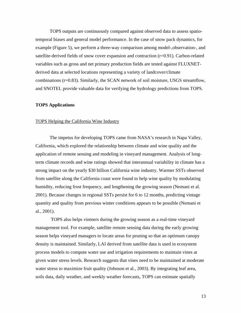
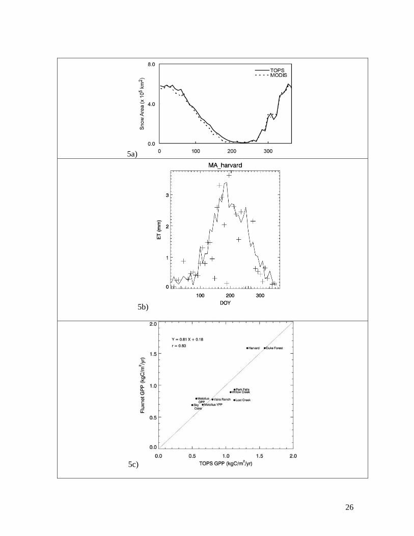
TOPS outputs are continuously compared against observed data to assess spatio-

temporal biases and general model performance. In the case of snow pack dynamics, for

example (Figure 5), we perform a three-way comparison among model-,observation-, and

satellite-derived fields of snow cover expansion and contraction (r=0.91). Carbon-related

variables such as gross and net primary production fields are tested against FLUXNET-

derived data at selected locations representing a variety of landcover/climate

combinations (r=0.83). Similarly, the SCAN network of soil moisture, USGS streamflow,

and SNOTEL provide valuable data for verifying the hydrology predictions from TOPS.

TOPS Applications

TOPS Helping the California Wine Industry

The impetus for developing TOPS came from NASA’s research in Napa Valley,

California, which explored the relationship between climate and wine quality and the

application of remote sensing and modeling in vineyard management. Analysis of long-

term climate records and wine ratings showed that interannual variability in climate has a

strong impact on the yearly $30 billion California wine industry. Warmer SSTs observed

from satellite along the California coast were found to help wine quality by modulating

humidity, reducing frost frequency, and lengthening the growing season (Nemani et al.

2001). Because changes in regional SSTs persist for 6 to 12 months, predicting vintage

quantity and quality from previous winter conditions appears to be possible (Nemani et

al., 2001).

TOPS also helps vintners during the growing season as a real-time vineyard

management tool. For example, satellite remote sensing data during the early growing

season helps vineyard managers to locate areas for pruning so that an optimum canopy

density is maintained. Similarly, LAI derived from satellite data is used in ecosystem

process models to compute water use and irrigation requirements to maintain vines at

given water stress levels. Research suggests that vines need to be maintained at moderate

water stress to maximize fruit quality (Johnson et al., 2003). By integrating leaf area,

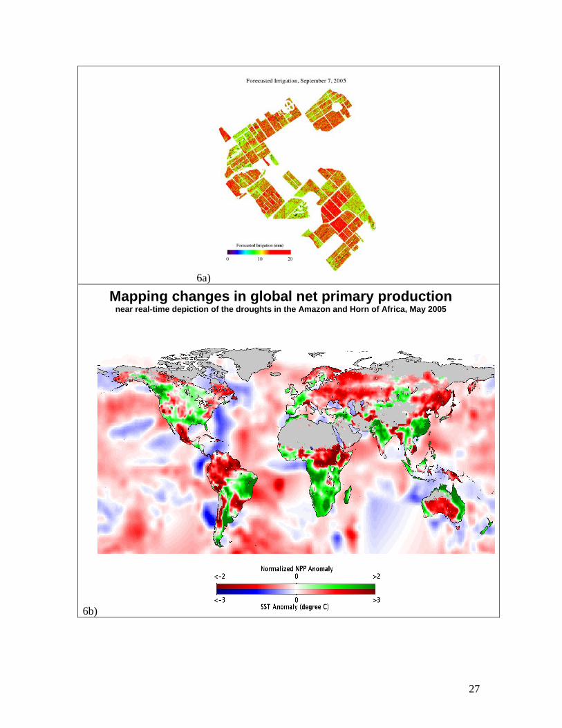
soils data, daily weather, and weekly weather forecasts, TOPS can estimate spatially

14

varying water requirements within the vineyard so that managers can adjust water

delivery from irrigation systems (Figure 6a). A number of Napa valley vintners presently

participate in our experimental irrigation forecast program, helping us verify the utility of

the forecasts, the packaging and delivery of information, and assess the economic value

of the forecasts. Satellite imagery at the end of the growing season also helps growers in

delineating regions of similar grape maturity and quality so that differential harvesting

can be employed to optimize wine blending and quality (Johnson et al. 2003).

TOPS monitors global ecosystems

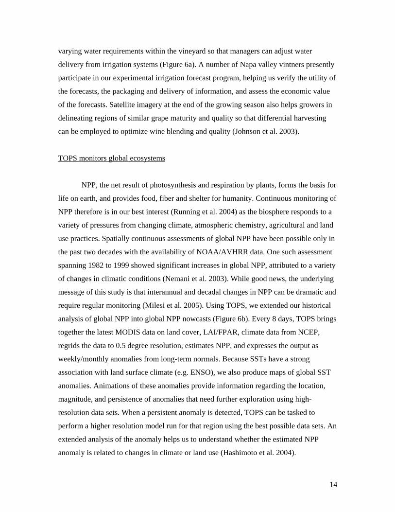
NPP, the net result of photosynthesis and respiration by plants, forms the basis for

life on earth, and provides food, fiber and shelter for humanity. Continuous monitoring of

NPP therefore is in our best interest (Running et al. 2004) as the biosphere responds to a

variety of pressures from changing climate, atmospheric chemistry, agricultural and land

use practices. Spatially continuous assessments of global NPP have been possible only in

the past two decades with the availability of NOAA/AVHRR data. One such assessment

spanning 1982 to 1999 showed significant increases in global NPP, attributed to a variety

of changes in climatic conditions (Nemani et al. 2003). While good news, the underlying

message of this study is that interannual and decadal changes in NPP can be dramatic and

require regular monitoring (Milesi et al. 2005). Using TOPS, we extended our historical

analysis of global NPP into global NPP nowcasts (Figure 6b). Every 8 days, TOPS brings

together the latest MODIS data on land cover, LAI/FPAR, climate data from NCEP,

regrids the data to 0.5 degree resolution, estimates NPP, and expresses the output as

weekly/monthly anomalies from long-term normals. Because SSTs have a strong

association with land surface climate (e.g. ENSO), we also produce maps of global SST

anomalies. Animations of these anomalies provide information regarding the location,

magnitude, and persistence of anomalies that need further exploration using high-

resolution data sets. When a persistent anomaly is detected, TOPS can be tasked to

perform a higher resolution model run for that region using the best possible data sets. An

extended analysis of the anomaly helps us to understand whether the estimated NPP

anomaly is related to changes in climate or land use (Hashimoto et al. 2004).

15

On-going applications of TOPS include nowcasting and forecasting of snow

dynamics in the Columbia River Basin (Northwestern U.S.), mapping fire risk across the

continental U.S., mapping NPP at 250m in protected areas such as U.S. National Parks,

carbon and water management in urban ecosystems (Milesi et al.,2005) , and monitoring

and forecasting mosquito abundance and outbreaks of West Nile virus in California.

TOPS products are available in WMS format so these data can be accessed and visualized

using NASA’s WorldWind (http://worldwind.arc.nasa.gov) software system designed

explicitly for educational purposes.

Summary

In the past, ecological forecasting has been largely anecdotal. Its transformation

into a rigorous, scientific endeavor is now possible through the observing capacity of

operational satellites, the speed and flexibility of the internet, the use of high-

performance computing for complex modeling of living systems, and mining of large

quantities of data in search of relations that could offer potential predictability. Unlike the

case of weather and climate forecasting, EF can be as diverse as the number of weather-

influenced phenomena. We hope our efforts at EF can provide the necessary guidance for

future applications, since the basic infrastructure needed to enable ecological forecasts

appears to be similar across different domains. Our experience with EF has been that

producing the forecasts may be the easy part, convincing users and conveying the

uncertainty associated with the forecasts has been a challenge. Much work is needed

along these lines to realize the full potential of ecological forecasting.

16

References L.E. Band, P. Patterson, R. Nemani and S.W. Running. 1993. Forest ecosystem processes at the

watershed scale: incorporating hill slope hydrology. Agricultural and Forest Meteorology, 63: 93-126.

Barnett, T.P., L. Bengtsson, K. Arpe, M. Flugel, N. Graham, M. Latif, J. Ritchie, E. Roeckner,

U. Schlese, U. Schulzweida, and M. Tyree. 1994: Forecasting global ENSO-related climate anomalies. Tellus, 46A, 381-397.

Cane, M. A. G. Eshel, and R.W. Buckland. 1994. Forecasting Zimbabwean maize yield using

eastern equatorial Pacific sea surface temperature. Nature, 370, 204 – 205. Canham, C.D., J.J. Cole, and W.K. Lauenroth. 1997. Models in ecosystem science. Princeton

University press, 456 pp. Clark, J.S., S.R. Carpenter, M. Barber, S. Collins, A. Dobson, J.A. Foley, D.M. Lodge, M.

Pascual, R. Pielke Jr., W. Pizer, C. Pringle, W.V. Reid, K.A. Rose, O. Sala, W.H. Schlesinger, D.H. Wall, and D. Wear. 2001. Ecological forecasts: An emerging imperative. Science 293: 657–660.

Daly, C., R.P. Neilson, and D.L. Phillips. 1994: A Statistical-Topographic Model for Mapping

Climatological Precipitation over Mountainous Terrain. Journal of Applied Meteorology, 33, 140-158.

Goddard, L., S. J. Mason, S. E. Zebiak, C. F. Ropelewski, R. Basher,and M. A. Cane. 2001. Current approaches to climate prediction. Int. J. Climatology, 21 (9): 1111-1152.

Golden, K., W. Pang, R. Nemani and P. Votava. 2003. Automating the processing of Earth

observation data. Proceedings of the 7th International Symposium on Artificial Intelligence, Robotics and Automation for Space (i-SAIRAS 2003), Nara, Japan. May 19-23.

Hashimoto H., R.R. Nemani, M.A. White, W.M. Jolly, S.C. Piper, C.D. Keeling, R.B. Myneni and S.W. Running. 2004. El Niño–Southern Oscillation–induced variability in terrestrial carbon cycling. Journal of Geophysical Research-Atmospheres, 109 (D23): D23110, doi:10.1029/2004JD004959.

Jolly, M., J.M. Graham, A. Michaelis, R. Nemani and S.W. Running. 2004. A flexible, integrated

system for generating meteorological surfaces derived from point sources across multiple geographic scales. Environmental modeling & software, 15: 112-121.

Johnson, L., D. Roczen, S. Youkhana, R.R. Nemani and D.F. Bosch. 2003. Mapping vineyard

leaf area with multispectral satellite imagery. Computers & Agriculture, 38(1): 37-48.

17

Justice, E. Vermote, J. R. G. Townshend, R. Defries, D. P. Roy, D.K. Hall, V. V. Salomonson, J. Privette, G. Riggs, A. Strahler, W. Lucht, R. Myneni, Y. Knjazihhin, S. Running, R. Nemani, Z. Wan, A. Huete, W. van Leeuwen, R. Wolfe, L. Giglio, J-P. Muller, P. Lewis, and M. Barnsley. 1998. The moderate resolution imaging spectroradiometer (MODIS): land remote sensing for global change research. IEEE Transactions on Geoscience and Remote Sensing, 36: 1228-1249.

Milesi, C., H. Hashimoto, S.W. Running and R. Nemani. 2005. Climate variability, vegetation

productivity and people at risk. Global and Planetary Change, 47: 221-231. Milesi, C., C.D. Elvidge, J.B. Dietz, B.J. Tuttle, R.R. Nemani, and S.W. Running. 2005.

Mapping and modeling the biogeochemical cycling of turf grasses in the United States. Environmental Management. Online First. DOI: 10.1007/s00267-004-0316-2.

Myneni, R.B., S. Hoffman, J. Glassy, Y. Zhang, P. Votava, R. Nemani and S. Running. 2002.

Global products of vegetation leaf area and fraction absorbed PAR from year one of MODIS data. Remote Sensing of Environment, 48(4): 329-347.

Nemani, R., S. Running, L. Band and D. Peterson. 1993. Regional Hydro-Ecological Simulation

System: An illustration of the integration of ecosystem models in a GIS. In: M.F. Goodchild, B.O. Parks and L. Steyeart (eds.), Environmental modeling and GIS, Oxford press, p. 296-304.

Nemani, R.R., M.A. White, D.R. Cayan, G.V. Jones, S.W. Running, J.C. Coughlan and D.L.

Peterson. 2001. Asymmetric warming along coastal California and its impact on the premium wine industry. Climate Research, 19: 25-34.

Nemani, R.R., C.D. Keeling, H. Hashimoto, W.M. Jolly, S.C. Piper, C.J. Tucker, R.B. Myneni

and S.W. Running. 2003. Climate driven increases in terrestrial net primary production from 1982 to 1999. Science, 300: 1560-1563. Proceedings of Earth Science Technology Conference, Maryland, August 28-30.

Running, S.W., R.R. Nemani, F.A. Heinsch, M. Zhao, M. Reeves and H. Hashimoto. 2004. A continuous satellite-derived measure of global terrestrial primary productivity. Bioscience, 54(6): 547-560.

Roads, S.-C. Chen, J.R.F. Fujioka, H. Juang, M. Kanamitsu. 1999. ECPC's global to regional

fireweather forecast system. Proceedings of the 79th Annual AMS Meeting, Dallas, TX January 10-16.

Robertson, A., U. Lall, S.E. Zebiak and L. Goddard, 2004. Improved combination of multiple atmospheric general circulation model ensembles for seasonal prediction. Monthly Weather Review, 132, 2732-2744.

Tague, C. and L. Band. 2004. RHESSys: Regional Hydro-ecologic simulation system: An

object-oriented approach to spatially distributed modeling of carbon, water and nutrient cycling. Earth Interactions, 8(19): 1-42.

18

Thomson, M. C., F. J. Doblas-Reyes, S. J. Mason, R. Hagedorn, S. J. Connor, T. Phindela, A. P. Morse, and T. N. Palmer, 2006: Malaria early warnings based on seasonal climate forecasts from multi-model ensembles. Nature, 439, 576-579.

Thornton, P.E., S.W. Running and M.A. White. 1997. Generating surfaces of daily meteorological variables over large regions of complex terrain. Journal of Hydrology, 190: 214-251.

Trenberth, K.E. 1996. Short-term climate variations: Recent accomplishments and issues for

future progress. Bull. Amer. Met. Soc., 78: 1081-1096. Waring, R. H. and S.W. Running. 1998. Forest Ecosystems: Analysis at Multiple Scales, 2nd

Edition. Academic Press. White, M.A., P.E. Thornton, S.W. Running and R.R. Nemani. 2000. Parameterization and

sensitivity analysis of the BIOME-BGC terrestrial ecosystem model: net primary production controls. Earth Interactions, 4: 1-85.

White, M.A. and R. R. Nemani. 2004. Soil water forecasting in the continental U.S. Canadian

Journal of Remote Sensing, 30(5): 1-14. Wood, A.W., E.P. Maurer, P. Edwin, A. Kumar, D.P. Lettenmaier, 2001, Long-range

experimental hydrologic forecasting for the eastern United States, Journal of Geophysical Research (Atmospheres), Volume 107, Issue D20, pp. ACL 6-1, CiteID 4429, DOI 10.1029/2001JD000659.

Zebiak, Stephen W, 2003: Research Potential for Improvements in Climate Prediction. Bull. Of

the Amer. Met. Society. 84(12), 1692-1696.

19

Figure Captions: Figure 1. The Terrestrial Observation and Prediction System (TOPS) integrates a wide variety of data sources at various space and time resolutions to produce spatially and temporally consistent input data fields, upon which ecosystem models operate to produce ecological nowcasts and forecasts needed by natural resource managers. Figure 2: TOPS data processing flowchart showing three key modules that perform data acquisition and pre-processing, data and model integration and decision support through analysis of model inputs and outputs. Application front-ends, predictive models, and data mining algorithms are modular and can be easily swapped out as needed. The modular architecture also allows for the concurrent use of multiple ecosystem models to generate forecasts for different parameters. Figure 3: Flow diagram of the SOGS. Three main components that comprise the system are: data retrieval and storage, interpolation and output handling. Data retrieval is configured to automatically retrieve the most recent data available and insert those data into the SQL database. Interpolation methods are modular and allow maximum flexibility in implementing new routines as they become available. Outputs are generated on the prediction grid that is determined by the latitude, longitude, elevation and mask layers. Another key feature of the SOGS implementation is scenario generation where long-term normal station data can be perturbed according to climate model forecasts. Weather data from over 6000 stations distributed globally is ingested into TOPS database where it is gridded to a variety of resolutions, globally at 0.5 degree, continental U.S at 8km and at 1km over California. Figure 4: Examples of TOPS nowcasts. a) Patterns of maximum air temperature over the conterminous U.S., produced using over 1400 stations on April, 27, 2004. b) MODIS-derived leaf area index after pre-processing through TOPS, and c) Model estimated gross primary production, the amount of photosynthate accumulated on April 27, 2004 over the conterminous U.S. Figure 5: Testing TOPS products against satellite and network observations: a) TOPS snow cover against MODIS-derived snow cover, b) TOPS Evapotranspiration against FLUXNET observations at Harvard Forest, and c) TOPS Gross Primary Production shown against FLUXNET observations at a number of sites across the U.S. Figure 6: a) Application of TOPS over Napa valley vineyards showing the recommended irrigation amounts to keep the vines at a stress level of –12bars for the week of September 7, 2004. b) A global application of TOPS for monitoring and mapping net primary production anomalies over land and sea surface temperature anomalies over global oceans. NPP and SST anomalies for May 2005 are based on monthly means from 1981-2000.

20

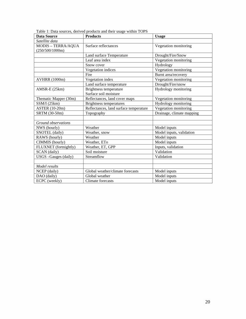
Table 1: Data sources, derived products and their usage within TOPS Data Source Products Usage Satellite data MODIS – TERRA/AQUA (250/500/1000m)

Surface reflectances Vegetation monitoring

Land surface Temperature Drought/Fire/Snow Leaf area index Vegetation monitoring Snow cover Hydrology Vegetation indices Vegetation monitoring Fire Burnt area/recovery AVHRR (1000m) Vegetation index Vegetation monitoring Land surface temperature Drought/Fire/snow AMSR-E (25km) Brightness temperature

Surface soil moisture Hydrology monitoring

Thematic Mapper (30m) Reflectances, land cover maps Vegetation monitoring SSM/I (25km) Brightness temperatures Hydrology monitoring ASTER (10-20m) Reflectances, land surface temperature Vegetation monitoring SRTM (30-50m) Topography Drainage, climate mapping Ground observations NWS (hourly) Weather Model inputs SNOTEL (daily) Weather, snow Model inputs, validation RAWS (hourly) Weather Model inputs CIMMIS (hourly) Weather, ETo Model inputs FLUXNET (fortnightly) Weather, ET, GPP Inputs, validation SCAN (daily) Soil moisture Validation USGS –Gauges (daily) Streamflow Validation Model results NCEP (daily) Global weather/climate forecasts Model inputs DAO (daily) Global weather Model inputs ECPC (weekly) Climate forecasts Model inputs

21

Acronyms AMSR-E Advanced Microwave Scanning Radiometer-Earth

Observing System ASTER Advanced Spaceborne Thermal Emission and Reflection

Radiometer AVHRR Advanced Very High Resolution Radiometer BIOME-BGC Biome-biogeochemistry CIMIS California Irrigation Management Information System DAAC Distributed Active Archive Center DAO Data Assimilation Office ECPC Experimental Climate Prediction Center EF Ecological Forecasting ENSO El Niño–Southern Oscillation ET Evapotranspiration ETo Reference Evapotranspiration FLUXNET Network of eddy covariance towers FPAR Fraction of Photosynthetic Active Radiation GCM General Circulation Model GOES Geostationary Operational Environmental Satellites GPP Gross Primary Production ImageBot heuristic-search constraint-based planner JDAF Java-based Distributed Application Framework

(executing plans and for interfacing with DAACs) DAPDL Data Processing Action Description Language WMS Web Map Server LAI MODIS MODerate resolution Imaging Spectro-radiometer NCEP National Center for Environmental Prediction NOAA National Oceanic and Atmospheric Administration NPP Net Primary Production NWS National Weather Service RAWS Remote Automated Weather Stations RHESSys Regional Hydro-Ecological Simulation System SCAN Soil Climate Analysis Network SNOTEL SNOWpack TELemetry network SOGS Surface Observation and Gridding System SRTM Shuttle Radar Topography Mission SSM/I Special Sensor Microwave Imager SST Sea surface temperature TOPS Terrestrial Observation and Prediction System USFS United States Forest Service USGS United States Geological Survey XML Extensible Markup Language

22

Figure 1:

23

INGEST

CO2 dataFLUXNEXT, Inventory,

Streamflow

Remote SensingEOS data/products

Point/Gridded climateobservations/forecasts

MODEL MANAGER

ApplicationsModels

Land SurfaceModels

Input ModelSpecification Interface

Interannual Variations/Trends

Output ModelSpecification Interface

Derived Biophysical Variables

-- A

-- A

-- A

-- A

-- A

-- A

-- A-- P

-- P

-- A

-- A

-- A -- A

-- A

-- A

-- A

-- A

-- P

-- P

-- P

Plan

ning

/Sch

edul

ing/

Exec

utio

nD

ata

Acq

uisi

tion

& P

re-p

roce

ssin

gD

ecis

ion

Supp

ort

anal

ysis

of r

esul

tsD

ata

and

Mod

el In

tegr

atio

nH

indc

asts

, Now

cast

s &

For

ecas

ts

SCALING {up or down}

TEMPORAL{hourly-to-daily}

FORMAL FILTERS.{wgrib, others}

SPATIAL REPROJECTION

Causal Mechanisms

Statistical summaries/Tables

TopographySoils

Figure 2:

24

Figure 3:

25

4a)

4b)

4c)

26

5a)

5b)

5c)

27

6a)

6b)

Mapping changes in global net primary productionnear real-time depiction of the droughts in the Amazon and Horn of Africa, May 2005