The 1990s in Japan: A Lost Decade*

Fumio HayashiUniversity of Tokyo

E-mail: hayashi@e.u-tokyo.ac.jp

Edward C. PrescottArizona State University

Research Department, Federal Reserve Bank of Minneapolis,Minneapolis, Minnesota 55480

E-mail: edward.prescott@asu.edu

October 2001, revised and expanded August 2003

*We thank Tim Kehoe, Nobu Kiyotaki, Ellen McGrattan and Lee Ohanian for helpful comments,and Sami Alpanda, Pedro Amaral, Igor Livshits, and Tatsuyoshi Okimoto for excellent researchassistance and the Cabinet Office of the Japanese government, the United States National ScienceFoundation, and the College of Liberal Arts of the University of Minnesota for financial support.The views expressed herein are those of the authors.

1

Abstract

This paper examines the Japanese economy in the 1990s, a decade of economic stagnation.

We find that the problem is not a breakdown of the financial system, as corporations large and

small were able to find financing for investments. There is no evidence of profitable investment

opportunities not being exploited due to lack of access to capital markets. The problem then

and still today, is a low productivity growth rate. Growth theory, treating TFP as exogenous,

accounts well for the Japanese lost decade of growth. We think that research effort should be

focused on what policy change will allow productivity to again grow rapidly. Journal of Economic

Literature Classification Numbers: E2, E13, O4, O5,

Key words: growth model, TFP, Japan, workweek

2

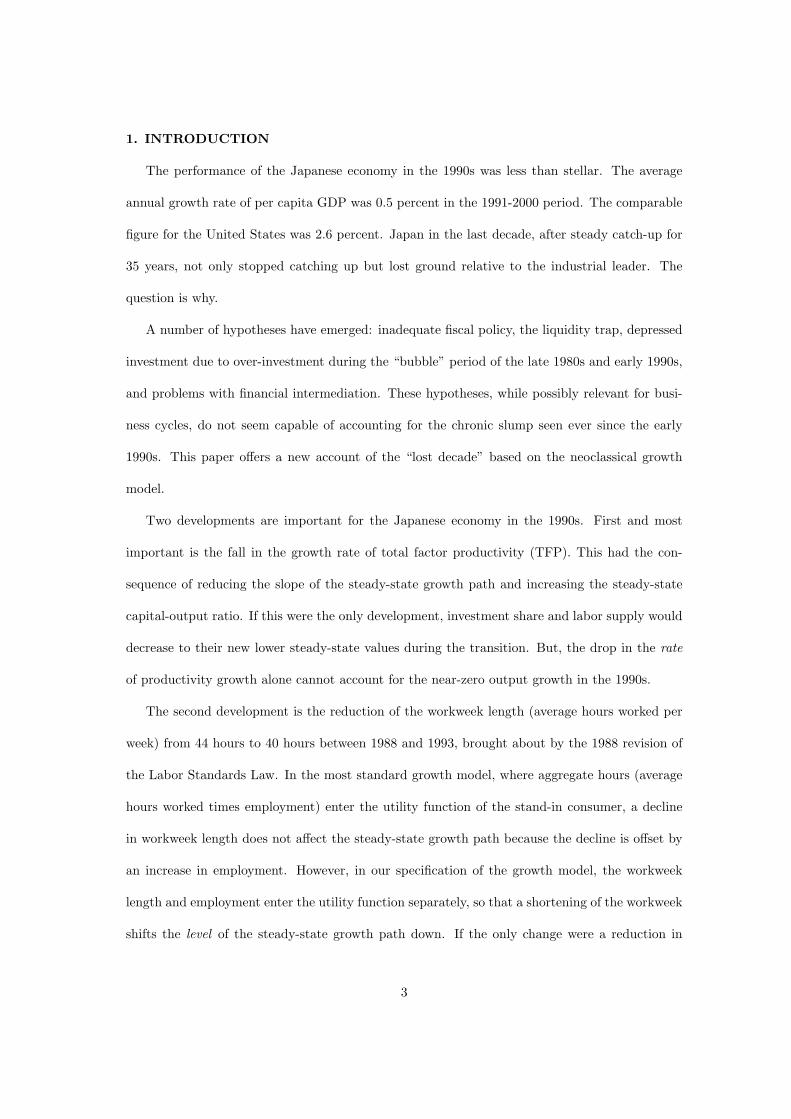
1. INTRODUCTION

The performance of the Japanese economy in the 1990s was less than stellar. The average

annual growth rate of per capita GDP was 0.5 percent in the 1991-2000 period. The comparable

figure for the United States was 2.6 percent. Japan in the last decade, after steady catch-up for

35 years, not only stopped catching up but lost ground relative to the industrial leader. The

question is why.

A number of hypotheses have emerged: inadequate fiscal policy, the liquidity trap, depressed

investment due to over-investment during the “bubble” period of the late 1980s and early 1990s,

and problems with financial intermediation. These hypotheses, while possibly relevant for busi-

ness cycles, do not seem capable of accounting for the chronic slump seen ever since the early

1990s. This paper offers a new account of the “lost decade” based on the neoclassical growth

model.

Two developments are important for the Japanese economy in the 1990s. First and most

important is the fall in the growth rate of total factor productivity (TFP). This had the con-

sequence of reducing the slope of the steady-state growth path and increasing the steady-state

capital-output ratio. If this were the only development, investment share and labor supply would

decrease to their new lower steady-state values during the transition. But, the drop in the rate

of productivity growth alone cannot account for the near-zero output growth in the 1990s.

The second development is the reduction of the workweek length (average hours worked per

week) from 44 hours to 40 hours between 1988 and 1993, brought about by the 1988 revision of

the Labor Standards Law. In the most standard growth model, where aggregate hours (average

hours worked times employment) enter the utility function of the stand-in consumer, a decline

in workweek length does not affect the steady-state growth path because the decline is offset by

an increase in employment. However, in our specification of the growth model, the workweek

length and employment enter the utility function separately, so that a shortening of the workweek

shifts the level of the steady-state growth path down. If the only change were a reduction in

3

workweek length, the economy would converge to a lower steady-state growth path subsequent

to the reduction in the workweek length.

We determine the consequence of these two factors for the behavior of the Japanese economy

in the 1990s. To do this we calibrate our growth model to pre-1990 data and use the model to

predict the path of the Japanese economy in the 1990s, treating TFP as exogenous and treating

the workweek length as endogenous subsequent to 1993. The lost decade of growth is what the

model predicts. Also predicted is the increase in the capital-output ratio and the fall in the return

on capital that occurred through the 1990s. The only puzzle is why the TFP growth was so low

subsequent to 1991. We discuss possible reasons for this decline in the concluding section of the

paper.

In Section 2, we start with a brief catalogue of some of the facts about the lost decade. We

then proceed to examine the Japanese economy through the perspective of growth theory in

Section 3. We use this model economy to predict what will happen in the 1990s and beyond,

taking the paths of productive efficiency, workweek lengths, capital tax rate, and the output share

of government purchases as exogenous.

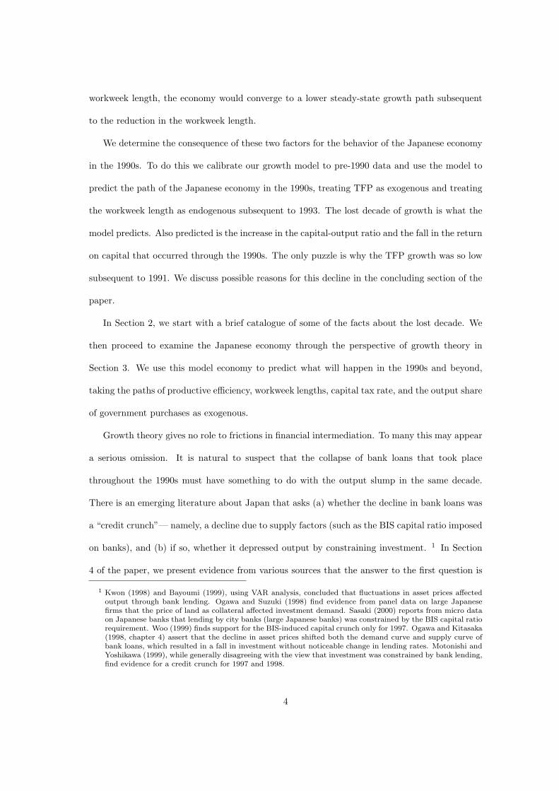
Growth theory gives no role to frictions in financial intermediation. To many this may appear

a serious omission. It is natural to suspect that the collapse of bank loans that took place

throughout the 1990s must have something to do with the output slump in the same decade.

There is an emerging literature about Japan that asks (a) whether the decline in bank loans was

a “credit crunch”— namely, a decline due to supply factors (such as the BIS capital ratio imposed

on banks), and (b) if so, whether it depressed output by constraining investment. 1 In Section

4 of the paper, we present evidence from various sources that the answer to the first question is

1 Kwon (1998) and Bayoumi (1999), using VAR analysis, concluded that fluctuations in asset prices affectedoutput through bank lending. Ogawa and Suzuki (1998) find evidence from panel data on large Japanesefirms that the price of land as collateral affected investment demand. Sasaki (2000) reports from micro dataon Japanese banks that lending by city banks (large Japanese banks) was constrained by the BIS capital ratiorequirement. Woo (1999) finds support for the BIS-induced capital crunch only for 1997. Ogawa and Kitasaka(1998, chapter 4) assert that the decline in asset prices shifted both the demand curve and supply curve ofbank loans, which resulted in a fall in investment without noticeable change in lending rates. Motonishi andYoshikawa (1999), while generally disagreeing with the view that investment was constrained by bank lending,find evidence for a credit crunch for 1997 and 1998.

4

probably yes, but the answer to the second question is no. That is, despite the collapse of bank

loans, firms found ways to finance investment. This justifies our neglect of financial factors in

accounting for the lost decade. Section 5 contains concluding remarks.

2. THE JAPANESE ECONOMY 1984-2000

We begin with an examination of the NIA (National Income Accounts) data for the 1984-2000

period and report the facts that are most germane to real growth theory, which abstracts from

monetary and financial factors. In the next section, we will determine the importance of the TFP

behavior and the reduction in the workweek length on the behavior of the Japanese economy in

the 1990s.

Poor Performance in the 1990s

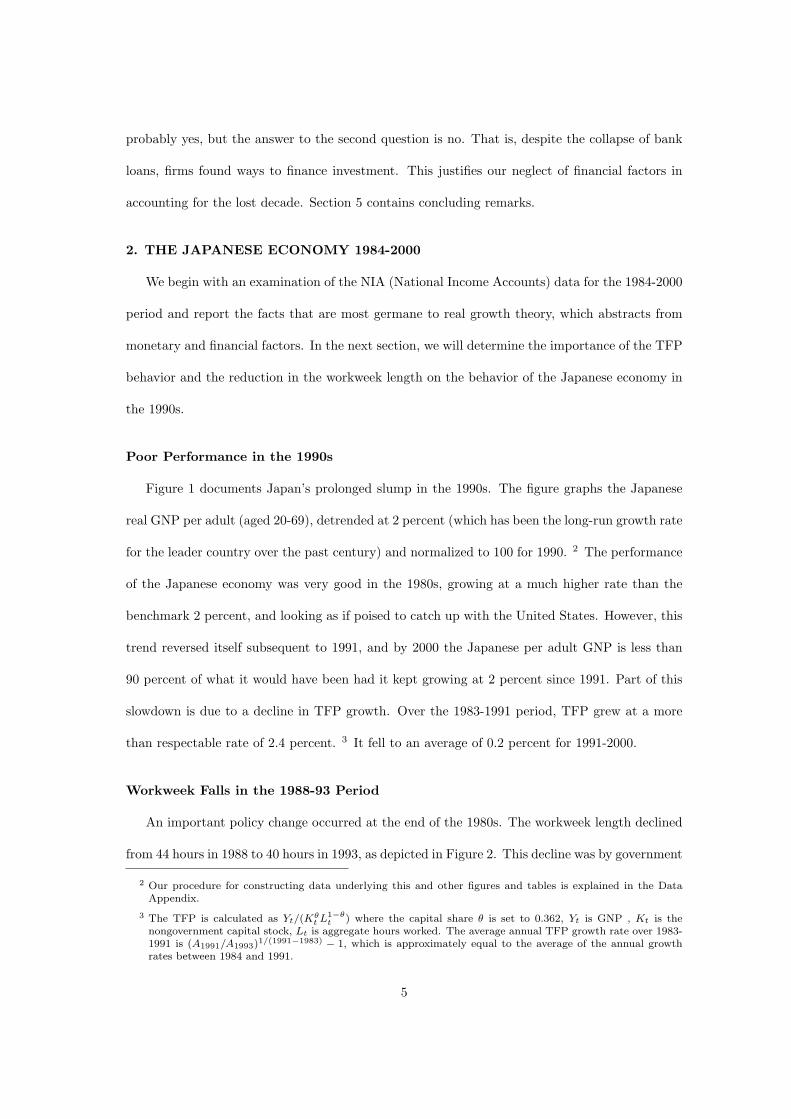
Figure 1 documents Japan’s prolonged slump in the 1990s. The figure graphs the Japanese

real GNP per adult (aged 20-69), detrended at 2 percent (which has been the long-run growth rate

for the leader country over the past century) and normalized to 100 for 1990. 2 The performance

of the Japanese economy was very good in the 1980s, growing at a much higher rate than the

benchmark 2 percent, and looking as if poised to catch up with the United States. However, this

trend reversed itself subsequent to 1991, and by 2000 the Japanese per adult GNP is less than

90 percent of what it would have been had it kept growing at 2 percent since 1991. Part of this

slowdown is due to a decline in TFP growth. Over the 1983-1991 period, TFP grew at a more

than respectable rate of 2.4 percent. 3 It fell to an average of 0.2 percent for 1991-2000.

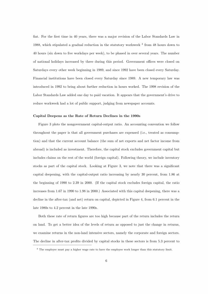
Workweek Falls in the 1988-93 Period

An important policy change occurred at the end of the 1980s. The workweek length declined

from 44 hours in 1988 to 40 hours in 1993, as depicted in Figure 2. This decline was by government

2 Our procedure for constructing data underlying this and other figures and tables is explained in the DataAppendix.

3 The TFP is calculated as Yt/(Kθt L1−θ

t ) where the capital share θ is set to 0.362, Yt is GNP , Kt is thenongovernment capital stock, Lt is aggregate hours worked. The average annual TFP growth rate over 1983-1991 is (A1991/A1993)1/(1991−1983) − 1, which is approximately equal to the average of the annual growthrates between 1984 and 1991.

5

fiat. For the first time in 40 years, there was a major revision of the Labor Standards Law in

1988, which stipulated a gradual reduction in the statutory workweek 4 from 48 hours down to

40 hours (six down to five workdays per week), to be phased in over several years. The number

of national holidays increased by three during this period. Government offices were closed on

Saturdays every other week beginning in 1989, and since 1992 have been closed every Saturday.

Financial institutions have been closed every Saturday since 1989. A new temporary law was

introduced in 1992 to bring about further reduction in hours worked. The 1998 revision of the

Labor Standards Law added one day to paid vacation. It appears that the government’s drive to

reduce workweek had a lot of public support, judging from newspaper accounts.

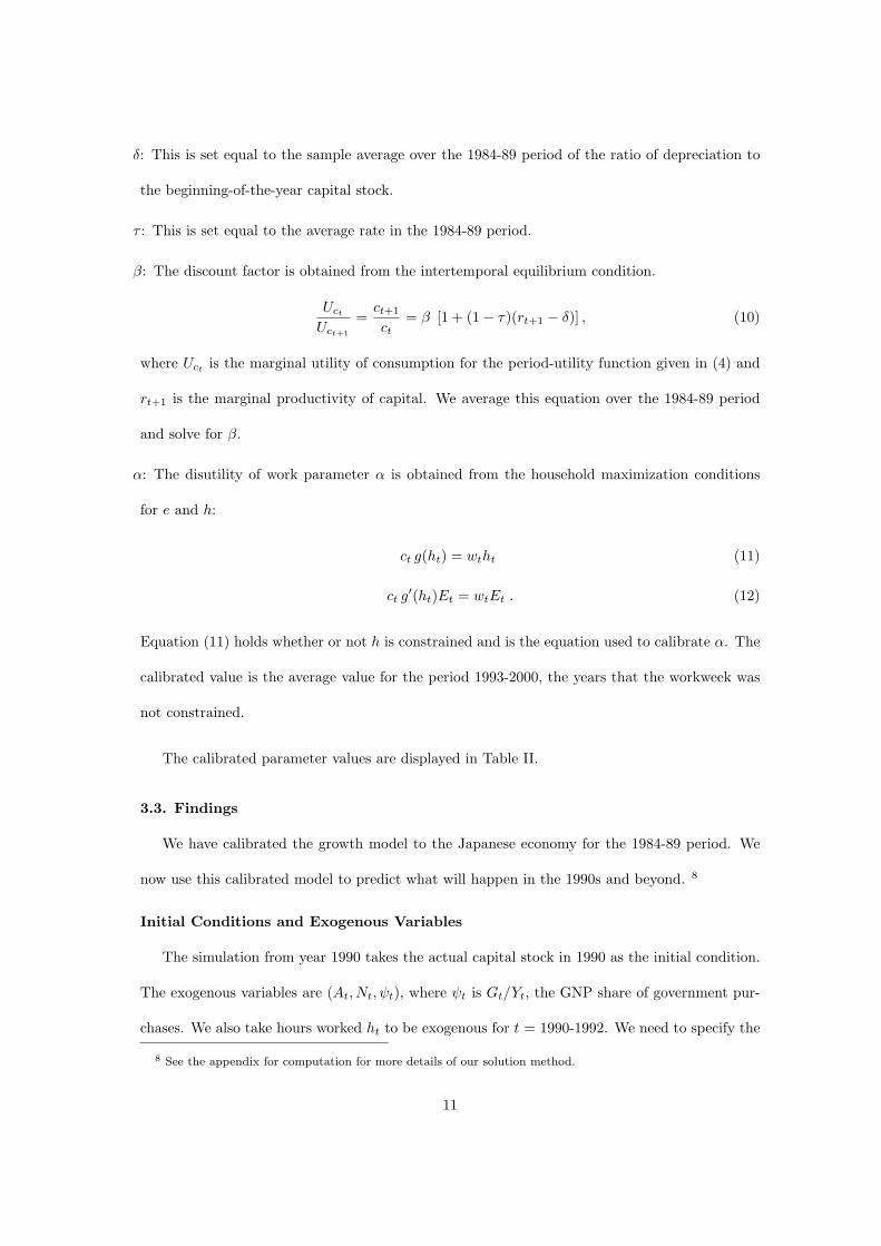
Capital Deepens as the Rate of Return Declines in the 1990s

Figure 3 plots the nongovernment capital-output ratio. An accounting convention we follow

throughout the paper is that all government purchases are expensed (i.e., treated as consump-

tion) and that the current account balance (the sum of net exports and net factor income from

abroad) is included as investment. Therefore, the capital stock excludes government capital but

includes claims on the rest of the world (foreign capital). Following theory, we include inventory

stocks as part of the capital stock. Looking at Figure 3, we note that there was a significant

capital deepening, with the capital-output ratio increasing by nearly 30 percent, from 1.86 at

the beginning of 1990 to 2.39 in 2000. (If the capital stock excludes foreign capital, the ratio

increases from 1.67 in 1990 to 1.98 in 2000.) Associated with this capital deepening, there was a

decline in the after-tax (and net) return on capital, depicted in Figure 4, from 6.1 percent in the

late 1980s to 4.2 percent in the late 1990s.

Both these rate of return figures are too high because part of the return includes the return

on land. To get a better idea of the levels of return as opposed to just the change in returns,

we examine returns in the non-land intensive sectors, namely the corporate and foreign sectors.

The decline in after-tax profits divided by capital stocks in these sectors is from 5.3 percent to

4 The employer must pay a higher wage rate to have the employee work longer than this statutory limit.

6

2.1 percent. This leads us to the assessment that the after-tax return on capital declined over

three percentage points between 1990 and 2000: from over 5 percent to about 2 percent.

Government Share Increases and Investment Share Decreases in the 1990s

Figure 5 shows that the composition of output changed in the 1990s. The government’s

share of output increased from an average share of 13.7 percent in the 1984-90 period to 15.2

percent in the 1994-2000 period. Another change is the decline in private investment share from

27.6 percent to 24.3 percent in these periods. Most of the decline in investment occurred in

the domestic investment component, not in the current account: the output share of domestic

investment declined by 3 percentage points, from 24.6 percent to 21.7 percent. The decline in

the late 1990s is rather substantial.

3. JAPANESE ECONOMY FROM THE GROWTH THEORY PERSPECTIVE

In using growth theory to view the Japanese economy in the 1990s, we are using a theory

that students of business cycles use to study business cycles and students of public finance use to

evaluate tax policies. The standard growth model, however, must be modified in one important

way to take into account the consequences of a policy change that led to a reduction in the average

workweek in Japan in the 1988-93 period. Taking as given the fall in the workweek length, the

fall in productivity growth, and the increase in the output share of government purchases in the

1990s, we use the theory to predict the path of the Japanese economy after 1990.

3.1. The Growth Model

Technology

The aggregate production function is

Y = A Kθ(h E)1−θ , (1)

where Y is aggregate output, A is TFP, K is aggregate capital, E is aggregate employment, and

h is hours per employee.

7

Growth Accounting

Having specified the aggregate production function, we can go back to the data on the

Japanese economy and perform growth accounting. Our growth accounting, involving the capital-

output ratio instead of the capital stock, is equivalent to, but differs in appearance from, the usual

growth accounting. Let N be the working-age population and define:

y ≡ Y/N, e ≡ E/N, x ≡ K/Y. (2)

Using these definitions on (1) and by simple algebra, we obtain

y = A1/(1−θ) h e xθ/(1−θ). (3)

That is, output per adult y can be decomposed into four factors: the TFP factor A1/(1−θ),

the workweek factor h, the employment rate factor e, and the capital intensity factor xθ/(1−θ).

Our growth accounting is convenient because the growth rate in the TFP factor coincides with

the trend growth rate of output per adult, namely the growth rate when hours worked h, the

employment rate e, and the capital output ratio x (= K/Y ) are constant.

Table I reports the growth rate of each of these factors for various subperiods since 1960.

The capital share parameter θ is set at 0.362 (see our discussion below on calibration). The

contribution of TFP growth between 1983-1991 and 1991-2000 accounts for nearly all the decline

in the growth in output per working-age-person. 5 In spite of the low TFP growth in the 1973-

83 period, output per adult increased at 2.2 percent. The reason that growth in output per

adult was higher in the 1973-83 period than in the 1991-2000 period is that in the earlier period

there was significantly more capital deepening and a smaller reduction in the labor input per

working-age-person.

Households

We model workweek length h as being exogenous prior to 1993 and endogenous thereafter.

Following Hansen (1985) and Rogerson (1988), labor is indivisible so that a person either works

5 The average annual TFP growth rate over 1983-1991, for example, is calculated as(A1991/A1983)1/(1991−1983) − 1.

8

h hours or does not work at all. There is a stand-in household with Nt working-age members at

date t. The size of the household evolves over time exogenously. Measure Et of the household

members work a workweek of length ht. The stand-in household utility function is

∞∑t=0

βtNt U(ct, ht, et) with U(ct, ht, et) = log ct − g(ht)et, (4)

where et ≡ Et/Nt is the fraction of household members that work and ct ≡ Ct/Nt is per member

consumption.

As policy decreased the workweek length over time, the disutility of working depends on h.

This disutility function is approximated in the neighborhood of h = 40 by a linear function 6

g(h) = α( 1 + (h− 40)/40 ). (5)

For this function, if not constrained, the workweek length chosen by the household is 40 hours.

This follows from household first-order conditions (11) and (12) below.

To incorporate taxes, we assume that the only distorting tax is a proportional tax on capital

income at rate τ . We could also incorporate a proportional tax on labor income. Provided that

the rate is constant over time, the labor tax does not affect any of our results. This is because

the labor tax, if included in the model, will be fully offset by a change in the calibrated value of

α (see the consumption-leisure first-order condition (11) and (12) below to see this point more

clearly). Since 1984 there has been no major tax reform affecting income taxes, it is reasonable to

assume that the average marginal tax rate on labor income (i.e., the marginal tax rates averaged

over different tax brackets) has been constant. We treat all other taxes as a lump-sum tax. The

resulting period-budget constraint of the household, which owns the capital and rents it to the

business sector, is

Ct +Xt 6 wthtEt + rtKt − τ (rt − δ)Kt − πt. (6)

Here wt represents the real wage, πt the lump sum taxes and rt is the rental rate of capital.

6 This function is proportional to h. See the appendix on computation for the reason.

9

The after-tax interest rate equals

it = (1− τ) (rt+1 − δ). (7)

The reason that we include a capital income tax is that a key variable in our analysis is the

after-tax return on capital and this return is taxed at a high rate in Japan, even higher than in

the United States.

Closing the Model

Aggregate output Yt is divided between consumption Ct, government purchases of goods and

services Gt, and investment Xt. 7 Thus

Ct +Xt +Gt = Yt. (8)

Capital depreciates geometrically, so

Kt+1 = (1− δ) Kt +Xt. (9)

The government budget constraint is implied by the household budget constraint (6) and the

resource constraint (8). By treating the capital tax income rate τ as a policy parameter, we are

assuming that changes in government purchases are financed by changes in the lump-sum tax πt.

Thus, Ricardian Equivalence holds in our model.

3.2. Calibration

We calibrate the model to the Japanese economy during 1984-89. There are five model

parameters: θ (capital share in production), δ (depreciation rate), β (discounting factor), α

(disutility of working), and τ (capital income tax rate). The data on the Japanese economy that

go into the following calibration (such as data on taxes on capital income) are described in the

Data Appendix.

θ: The share parameter is determined in the usual way, as the sample average over the period

1984-89 of the capital income share in GNP.

7 Recall that in our accounting framework government investment is included in G and that investment consistsof domestic private investment and the current account surplus. Hence (8) holds with Yt representing GNP.

10

δ: This is set equal to the sample average over the 1984-89 period of the ratio of depreciation to

the beginning-of-the-year capital stock.

τ : This is set equal to the average rate in the 1984-89 period.

β: The discount factor is obtained from the intertemporal equilibrium condition.

Uct

Uct+1

=ct+1

ct= β [1 + (1− τ)(rt+1 − δ)] , (10)

where Uct is the marginal utility of consumption for the period-utility function given in (4) and

rt+1 is the marginal productivity of capital. We average this equation over the 1984-89 period

and solve for β.

α: The disutility of work parameter α is obtained from the household maximization conditions

for e and h:

ct g(ht) = wtht (11)

ct g′(ht)Et = wtEt . (12)

Equation (11) holds whether or not h is constrained and is the equation used to calibrate α. The

calibrated value is the average value for the period 1993-2000, the years that the workweek was

not constrained.

The calibrated parameter values are displayed in Table II.

3.3. Findings

We have calibrated the growth model to the Japanese economy for the 1984-89 period. We

now use this calibrated model to predict what will happen in the 1990s and beyond. 8

Initial Conditions and Exogenous Variables

The simulation from year 1990 takes the actual capital stock in 1990 as the initial condition.

The exogenous variables are (At, Nt, ψt), where ψt is Gt/Yt, the GNP share of government pur-

chases. We also take hours worked ht to be exogenous for t = 1990-1992. We need to specify the

8 See the appendix for computation for more details of our solution method.

11

time path of those exogenous variables from 1990 on. For the 1990s (t = 1990, 1991, ... , 2000),

we use their actual values. For t = 2001, 2002, . . . , we assume the following. The TFP factor

A1/(1−θ)t is set to its 1991-2000 average of 0.29 percent. We assume no population growth so that

Nt is set to its 2000 value. The government’s share ψt is set equal to its value in the 1999-2000

period of 15 percent.

Our simulation is deterministic. The issue of what TFP growth expectations to assign to

the economic agents is problematic. We do not maintain that the decline in the growth rate of

the TFP factor in the 1990s was forecasted in 1990, even though we treat it as if it were. The

justification is that a deterministic model is simple and suffices for answering our question of

why the 1990s was a lost decade for the Japanese economy. If expectations had been modeled

in any not unreasonable way, the key predictions of the model would be essentially the same. In

particular, the magnitudes of the increase in the capital-output ratio and the fall in the return

on capital would be the same.

Figures 6-8 report the behavior of the model and actual outcomes. As can be seen from Figure

6, the actual output in the 1990-2000 period is close to the predictions of our calibrated model.

Theory with TFP exogenous predicts Japan’s chronic slump in the 1990s.

The observed deepening of capital and the decline in the rate of return, noted in Section 2

and reproduced in Figures 7 and 8, are also predicted by the model. The capital-output ratio

rises as output growth falls because the capital-output ratio associated with a lower productivity

growth is higher. This can easily be seen from equation (10). In the new steady state with

lower productivity growth, the consumption growth rate is lower, which means that the rate of

return from capital is lower. Under diminishing returns to capital, the capital-output ratio must

therefore be higher.

The difference in the precise paths of the model and actual path of the capital-output ratio

is not bothersome given the model’s assumption that the future path of the TFP factor was

predicted perfectly by the economic agents when in fact it is not. Neither is the discrepancy

12

between model and actual returns in Figure 8 bothersome. This is as expected given actual

returns include return on land as well as capital as discussed in Section 2.

The model’s predictions for the 1990s are not sensitive to the values of the exogenous variables

for the years beyond 2000. The predictions for the first decade of the twenty-first century, however,

depend crucially on the values of the exogenous parameters for that decade. The most important

variable is TFP. If the TFP growth rate increases to the historical norm of the industrial leader,

Japan will not fall further behind the leader — rather, it will maintain its position relative to the

industrial leader. If on the other hand, TFP growth is more rapid than the leader, Japan will

catch back up. We make no forecasts as to what TFP growth will be, and emphasize that this

forecast is conditional on the TFP growth rate remaining low.

Assuming that TFP growth remains low, Japan cannot rely on capital deepening for growth

in per-working-age-person output as it did in the past, as the Japanese capital stock is near its

steady-state value. On the other hand, decreases in the labor input (aggregate hours) will not

reduce growth as it has in the past, because, under our specification (5), average hours worked

h will not magnify the disutility of aggregate hours worked when it is less than 40 hours. The

Japanese people now work approximately the same number of hours as do Americans. If TFP

growth again becomes as rapid as it was in the 1983-1991 period, the labor input will increase

and this will have a positive steady-state level effect on output.

4. WAS INVESTMENT CONSTRAINED?

An important alternative hypothesis about Japan’s lost decade is what we call the “credit

crunch” hypothesis. It holds that, for one reason or another, there is a limit on the amount a firm

can borrow. If bank loans and other means of investment finance are not perfect substitutes, an

exogenous decrease in the loan limit constrains investment and hence depresses output. 9 This

hypothesis is becoming an accepted view even among academics. It has an appeal because the

collapse of bank loans and the output slump occurred in the same period (the 1990s) and because

9 See, e.g., Kashyap and Stein (1994) for a fuller statement of the hypothesis.

13

the collapse of bank loans seems exogenous, taking place when the BIS capital ratio is said to be

binding for many Japanese banks. In this section, we confront this “credit crunch” hypothesis

with data from various sources.

4.1. Evidence from the National Accounts

As mentioned at the end of Section 2, the output share of domestic investment declined

substantially in the 1990s. If this decline is due to reduced bank lending, we should see much

of the decline in investment by nonfinancial corporations. The Japanese National Accounts has

a flow-of-funds account (called the capital transactions account) for the nonfinancial corporate

sector that allows us to examine sources of investment finance. The cash flow identity for firms

states that

investment (excluding inventory investment)

= (a) net increase in bank loans

+ (b) net sales of land

+ (c) gross corporate saving (i.e., retention plus accounting depreciation)10

+ (d) net increase in other liabilities

(i.e., new issues in shares and corporate bonds plus net decrease in financial assets).

(13)

The capital transactions account in the Japanese National Accounts allows one to calculate items

(a)-(d) above for the nonfinancial corporate sector. 11

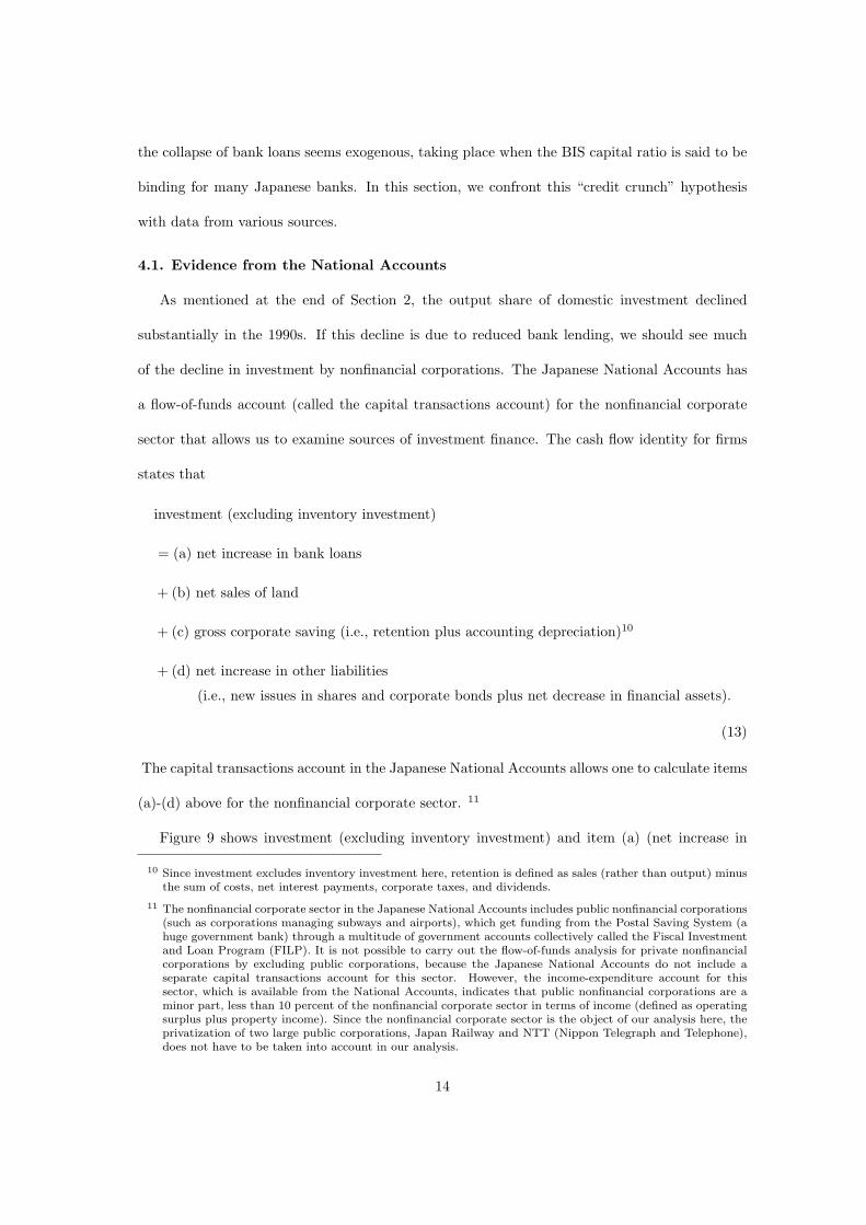
Figure 9 shows investment (excluding inventory investment) and item (a) (net increase in

10 Since investment excludes inventory investment here, retention is defined as sales (rather than output) minusthe sum of costs, net interest payments, corporate taxes, and dividends.

11 The nonfinancial corporate sector in the Japanese National Accounts includes public nonfinancial corporations(such as corporations managing subways and airports), which get funding from the Postal Saving System (ahuge government bank) through a multitude of government accounts collectively called the Fiscal Investmentand Loan Program (FILP). It is not possible to carry out the flow-of-funds analysis for private nonfinancialcorporations by excluding public corporations, because the Japanese National Accounts do not include aseparate capital transactions account for this sector. However, the income-expenditure account for thissector, which is available from the National Accounts, indicates that public nonfinancial corporations are aminor part, less than 10 percent of the nonfinancial corporate sector in terms of income (defined as operatingsurplus plus property income). Since the nonfinancial corporate sector is the object of our analysis here, theprivatization of two large public corporations, Japan Railway and NTT (Nippon Telegraph and Telephone),does not have to be taken into account in our analysis.

14

bank loan balances) as ratios to GNP. (The difference between the two, of course, is the sum of

items (b), (c), and (d).) There are two things to observe. First, the dive in the output share

of domestic investment, shown in Figure 5, did not occur in the nonfinancial corporate sector.

The output share of investment by nonfinancial corporations remained at 15 percent, except

for the “bubble” period of the late 1980s and early 1990s when the share was higher. Second,

investment held up despite the collapse of bank loans in the 1990s. 12 That is, other sources

of funds replaced bank loans to finance the robust investment by nonfinancial corporations in

the 1990s. To corroborate on this second point, Table III shows how the sources of investment

finance changed from 1984-88 to 1993-99 (thus excluding the “bubble” period). In the 1980s,

bank loans and gross corporate saving financed not only investment but also purchases of land

(see the negative entry for “sale of land” in the Table) and a buildup of financial assets (see the

negative entry for “net increase in other liabilities”). In the 1990s, firms drew down the land and

financial assets that had been built up during the 80s to support investment. These observations

are inconsistent with the “credit crunch” hypothesis.

4.2. Evidence from Survey Data on Private Nonfinancial Corporations

The preceding discussion, based on the National Accounts data, ignores distributional aspects.

For example, large firms may not have been constrained while small ones were. As is well known

(see, e.g., Hoshi and Kashyap (1999)), as a result of the liberalization of capital markets, large

Japanese firms scaled back their bank borrowing and started to rely more heavily on open-market

funding, and the shift away from bank loans is complete by 1990. It is also well known that for

small firms, essentially the only source of external funding is still bank loans. Therefore, if

investment is constrained for some firms, those firms must be small firms. How did the collapse

of bank loans affect small firms?

The most comprehensive survey of private nonfinancial corporations (a subset of the nonfi-

nancial corporate sector examined above) in Japan is a survey by the Ministry of Finance (MOF).

12 Bank loans here include loans made by public financial institutions. If loans from public financial institutionsare not included, the decline in bank lending in the 1990s is more pronounced.

15

13 From annual reports of this survey published by the MOF, sample averages of various income

and balance sheet variables for “small” firms (whose paid-in capital is less than 1 billion yen)

can be obtained for fiscal years (a Japanese fiscal year is from April of the year to March of the

next year). Figure 10 is the small-firm version of Figure 9. The difference between investment

and bank loans in the 1980s is much smaller in Figure 10 than in Figure 9, underscoring the

importance of bank loans for small firms. In the 1990s, however, as in Figure 9, investment held

firm in spite of the collapse of bank loans. The sources of investment finance for small firms

are shown in Table IV. It is not meaningful in the MOF survey to distinguish between items (c)

(gross saving) and (d) (net increase in liabilities other than bank loans) in the cash-flow iden-

tity (13). For example, suppose the firm reports hitherto unrealized capital gains on financial

asset holdings by selling those assets and then immediately buying them back. This operation

increases (c) and decreases (d) by the same amount. Therefore, in Table IV, items (c) and (d) are

bundled into a single item called “other.” The Table shows that small firms, despite the collapse

of bank loans, continued to increase land holdings in the 1990s. That is, gross corporate saving

and net decreases in financial assets combined were enough to finance not only the robust level

of investment but also land purchases — as all the while the loan balance was being reduced.

As just noted, it is not possible to tell from the MOF survey which component — saving or a

running down of assets — contributed more. It is, however, instructive to examine the evolution

of a component of financial assets whose reported value cannot be distorted by inclusion of

unrealized capital gains. Figure 11 graphs the ratio of cash and deposits to the (book value of)

capital stock. First of all, the ratio is huge. The ratio for the nonfinancial corporate sector as a

whole in the Japanese National Accounts is about 0.4. In contrast, the U.S. ratio for nonfinancial

corporations is much lower, less than 0.2, according to the Flow of Funds Accounts compiled by

the Board of Governors. For some reason the ratio was high in the early 1980s. 14 It is clear

13 See the Data Appendix for more details on this MOF survey.

14 Some of the cash and deposits must be compensating balances. We do not have statistics on compensatingbalances, however.

16

from this and previous figure that small firms during the “bubble” period used the cash and bank

loans for financial investments. Second, turning to the mid to late 1990s, Figure 10 indicates that

small firms relied on cash and deposits as a buffer against the steep decline in bank loans.

4.3 Evidence from Cross-Section Regressions

In the early 1990s, there was an active debate in the United States about whether the recession

in that period was due to a credit crunch. To answer this question, Bernanke and Lown (1991)

examined evidence from the U.S. states on output and loan growth. Based on a variety of

evidence, including a cross-section regression involving output and loan growth by state, they

concluded that the answer is probably no. In this subsection, we estimate the same type of

regression for the 47 Japanese prefectures.

For the recession period of 1990-91, Bernanke and Lown (1991) find that employment growth

in each state is related to contemporaneous growth in bank loans, with the bank loan regression

coefficient of 0.207 with a t value of over 3. A positive coefficient in the regression admits two

interpretations. The first is the “credit crunch” hypothesis that an exogenous decline in loan

supply constrains investment and hence output. The second is that the observed decline in bank

loans is due to a shift in loan demand. Bernanke and Lown (1991) prefer the second interpretation

because the positive coefficient became insignificant when loan growth is instrumented by the

capital ratio.

For Japan, we have available GDP by prefecture for fiscal years (April to March of the following

year) and loan balance (to all firms and also to small firms whose paid-in capital is 100 million

yen or less) at the end of March of each year. 15 The regression we run across prefectures is

GDP growth rate = β0 + β1 · bank loan growth rate. (14)

According to the official dating of business cycles (published by the ESRI (Economic and Social

Research Institute of the Cabinet Office of the Japanese government), there were five recessions

15 See the Data Appendix for more details.

17

since 1975: from March 1977 to October 1977, from February 1980 to February 1983, from June

1985 to November 1986, from February 1991 to October 1993, and from March 1997 to April

1999. Without monthly data, it is not possible to align these dates with our data on GDP and

bank loans. We therefore focus on the three longer recessions.

Our results are reported in Table V. In the regression for 1996-98, for example, the dependent

variable is GDP growth from fiscal year 1996 (April 1996 - March 1997) to fiscal year 1998 (April

1998 - March 1999). This GDP growth is paired with the growth in loan balance from March

1996 to March 1998. 16 The loan growth is for all firms in Regression 1 and for small firms

in Regression 2. Regression 1 is comparable to the state-level regression in Bernanke and Lown

(1991) for the U.S. states, except that the measure of output growth here is GDP growth, not

employment growth. 17 Overall, the loan growth coefficient is not significant, which is consistent

with our view that there may have been a credit crunch but it didn’t matter for investment

because firms found other ways to finance investment.

The significant coefficient for 1996-98 suggests that the recession in the late 1990s was partly

due to a credit crunch, but this period is special. The three-month commercial paper rate, which

has been about 0.5 to 0.6 percent since January 1996, shot up to above 1 percent in December 1997

and stayed near or above 1 percent before coming down to the 0.5 to 0.6 percent range in April

1998. During this brief period, various surveys of firms (for example, the Bank of Japan’s survey

called Tankan Survey) report a sharp rise in the fraction of small firms that said it was difficult

to borrow from banks. The regression result in Table V, which detects a significant association

between output and bank loans for 1996-98 but not for other periods, gives us confidence that

the “credit crunch” hypothesis, while possibly relevant for output for a few months from late

16 If the loan growth from March 1997 to March 1999 is used instead, the t value on loan growth is much smaller.

17 Published data on employment by prefecture are available for Japan, but only for manufacturing and at theends of calendar years. When we replaced GDP growth by employment growth in the regression, the loangrowth coefficient was less significant. For example, if employment growth from December 1996 to December1998 replaces the GDP growth from 1996-98, the t value on the loan growth coefficient is 0.35. Furthermore,in this employment growth equation, if the loan growth is for manufacturing firms, the loan growth coefficientis negative and insignificant.

18

1997 to early 1998, cannot account for the decade-long stagnation. 18

5. Concluding Comments

In examining the virtual stagnation that Japan began experiencing in the early 1990s, we find

that the problem is not a breakdown of the financial system, as corporations large and small were

able to find financing for investments. There is no evidence of profitable investment opportunities

not being exploited due to lack of access to capital markets. Those projects that are funded are

on average receiving a low rate of return.

The problem is low productivity growth. If it remains lower in Japan than in the other

advanced industrial countries, Japan will fall further behind. We are not predicting that this will

happen and would not be surprised if Japanese productivity growth returned to its level in the

1984-89 period. We do think that research effort should be focused on determining what policy

reform will allow productivity to again grow rapidly.

We can only conjecture on what reforms are needed. Perhaps the low productivity growth is

the result of a policy that subsidizes inefficient firms and declining industries. This policy results

in lower productivity because the inefficient producers produce a greater share of the output.

This also discourages investments that increase productivity. Some empirical support for this

subsidizing hypothesis is provided by the experience of the Japanese economy in the 1978-83

period. During that five-year period that the 1978 “Temporary Measures for Stabilization of

Specific Depressed Industries” law was in effect (see Peck, et al., 1988), the TFP growth rate was

a dismal 0.64 percent. In the three years prior, the TFP growth averaged 2.18 percent and in

6-year period after, it averaged slightly over 2.5 percent.

We said very little about the “bubble” period of the late 1980s and early 1990s, a boom

period when property prices soared, investment as a fraction of GDP was unusually high, and

output grew faster than in any other years in the 1980s and 1990s. We think the unusual pickup

18 Our view that the credit crunch hypothesis is applicable only for the brief period of late 1997 through early1998 is in accord with the general conclusion of the literature cited in footnote 1, particulary Woo (1999) andMotonishi and Yoshikawa (1999).

19

in economic activities, particularly investment, was due to an anticipation of higher productivity

growth that never materialized. To account for the bubble period along these lines, we need to

have a model where productivity is stochastic and where agents receive an indicator of future

productivity. But the account of the lost decade by such a model would be essentially the same

as the deterministic model used in this paper.

20

Data Appendix

This appendix is divided into two parts. In the first part, we describe in detail how we

constructed the model variables used in our neoclassical growth model. The second part describes

how the data underlying the tables and figures in the text are constructed. All the data are in

Excel files downloadable from http://www.e.u-tokyo.ac.jp/~hayashi/hp.

Part 1. Construction of Model Variables

The construction can be divided into two steps. The first is to make adjustments to the

data from the Japanese National Accounts, which is our primary data source, to make them

consistent with our theory. The second step is to calculate model variables from the adjusted

national accounts data and other sources. The exact formulas of these steps can be found in the

Excel file “rbc.xls” downloadable from the URL mentioned above.

Step 1: Adjustment to the National Accounts

Various adjustments to the Japanese National Accounts are needed for three reasons. First,

depreciation in the Japanese National Accounts is on historical cost basis. Second, in our theory

all government purchases are expensed. Third, starting in 2001 the Japanese National Accounts

(compiled by the ESRI (Economic and Social Research Institute, Cabinet Office of the Japanese

government)) adopted a new standard (called the 1993 SNA (System of National Accounts)

standard) that is different from the previous standard (the 1968 SNA).

Extension to 1999 and 2000. For years up to 1998, the 2000 Annual Report on National

Accounts has consistent series under the 1968 SNA standard. The 2001 Annual Report, which

adopted the 1993 SNA standard, has series only for 1991-1999. The ESRI also releases series on

the 1968 SNA basis for years up to 2000, but those series are only for a subset of the variables

forming the income and product accounts. Furthermore, those accounts divide the whole economy

into subsectors in a way different from the sector division in the 2000 Annual Report. From these

three sources, it is possible, under the usual sort of interpolation and extrapolation, to construct

consistent series for all relevant variables under the 1968 SNA standard up to 2000 (consult the

Excel file mentioned above for more details). On the left side of Table A-I, we report values

(relative to GNP) of items in the income and product accounts thus extended to 2000, averaged

over 1984-2000. Also reported are capital stocks relative to GNP. Beginning-of-year (end-of-

previous year) capital stocks for years up to 1999 are directly available from the 2000 Annual

Report ; capital stocks at the beginning of 2000 are taken from the 2001 Annual Report.

Capital consumption adjustments. The Japanese National Accounts include the bal-

ance sheets as well as the income and product accounts for the subsectors of the economy. In

the income and product accounts, depreciation (capital consumption) is on historical cost basis,

while in the balance sheets, capital stocks are valued at replacement costs. As was pointed out

in Chapter 11 of Hayashi (1997), replacement cost depreciation implicit in the balance sheets can

be estimated – under a certain set of assumptions – from various accounts included in the Na-

tional Accounts. For years up to 1998, this Hayashi estimation of replacement cost depreciation

21

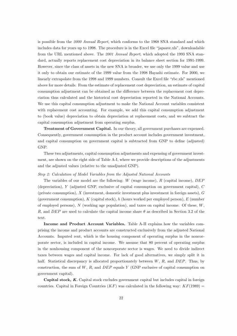
is possible from the 2000 Annual Report, which conforms to the 1968 SNA standard and which

includes data for years up to 1998. The procedure is in the Excel file “japsave.xls”, downloadable

from the URL mentioned above. The 2001 Annual Report, which adopted the 1993 SNA stan-

dard, actually reports replacement cost depreciation in its balance sheet section for 1991-1999.

However, since the class of assets in the new SNA is broader, we use only the 1999 value and use

it only to obtain our estimate of the 1999 value from the 1998 Hayashi estimate. For 2000, we

linearly extrapolate from the 1998 and 1999 numbers. Consult the Excel file “rbc.xls” mentioned

above for more details. From the estimate of replacement cost depreciation, an estimate of capital

consumption adjustment can be obtained as the difference between the replacement cost depre-

ciation thus calculated and the historical cost depreciation reported in the National Accounts.

We use this capital consumption adjustment to make the National Account variables consistent

with replacement cost accounting. For example, we add this capital consumption adjustment

to (book value) depreciation to obtain depreciation at replacement costs, and we subtract the

capital consumption adjustment from operating surplus.

Treatment of Government Capital. In our theory, all government purchases are expensed.

Consequently, government consumption in the product account includes government investment,

and capital consumption on government capital is subtracted from GNP to define (adjusted)

GNP.

These two adjustments, capital consumption adjustments and expensing of government invest-

ment, are shown on the right side of Table A-I, where we provide descriptions of the adjustments

and the adjusted values (relative to the unadjusted GNP).

Step 2: Calculation of Model Variables from the Adjusted National Accounts

The variables of our model are the following: W (wage income), R (capital income), DEP

(depreciation), Y (adjusted GNP, exclusive of capital consumption on government capital), C

(private consumption), X (investment, domestic investment plus investment in foreign assets), G

(government consumption), K (capital stock), h (hours worked per employed person), E (number

of employed persons), N (working age population), and taxes on capital income. Of these, W ,

R, and DEP are used to calculate the capital income share θ as described in Section 3.2 of the

text.

Income and Product Account Variables. Table A-II explains how the variables com-

prising the income and product accounts are constructed exclusively from the adjusted National

Accounts. Imputed rent, which is the housing component of operating surplus in the noncor-

porate sector, is included in capital income. We assume that 80 percent of operating surplus

in the nonhousing component of the noncorporate sector is wages. We need to divide indirect

taxes between wages and capital income. For lack of good alternatives, we simply split it in

half. Statistical discrepancy is allocated proportionately between W , R, and DEP . Thus, by

construction, the sum of W , R, and DEP equals Y (GNP exclusive of capital consumption on

government capital).

Capital stock, K. Capital stock excludes government capital but includes capital in foreign

countries. Capital in Foreign Countries (KF ) was calculated in the following way: KF (1989) =

22

25 * Net Factor Payments(1989), KF (t+1) =KF (t) + Net Exports(t) + Net Factor Payments(t).

Average hours worked, h. This variable is from an establishment survey conducted by

the Ministry of Welfare and Labor (this survey is called Maitsuki Kinro Tokei Chosa). We use a

series, included in this survey, for establishments with 30 or more employees. (There is a series

for establishments with 5 or more employees, but this series is available only since 1990.)

Employment, E . The number of employed persons for1970-98 is available from the National

Accounts (see Table I-[3]-3 of the 2000 Annual Report on National Accounts). The Labor Force

Survey (compiled by the General Affairs Agency) provides a different estimate of employment

from 1960 to the present. To extend the estimate in the NIA back to 1960, we multiply the Labor

Force Survey series by the ratio of the National Accounts estimate to the Labor Force Survey

estimate for 1970.

Working-age Population, N . The working-age population is defined as the number of

people between ages 20 and 69.

Taxes on Capital Income. This variable is used to calculate the tax rate on capital

income, denoted τ in the text. It is defined as the sum of direct taxes on corporate income

(available from the income account for the corporate sector in the National Accounts), 50 percent

of indirect business taxes, and 8 percent of operating surplus in the nonhousing component of

the noncorporate sector.

Part 2. Data Underlying Tables and Figures

Figures 1-5 and Table I use the model variables described in Part 1 of this appendix. Figures

6-8 are based on the simulation described in Section 3 of the text. The underlying data are in

Excel file “rbc.xls”.

Figure 9. Data on investment and bank loans are from the capital transactions account for

nonfinancial corporations in the Japanese National Accounts (Table 1-[2]-III-1). For 1984-98, the

data are from the 2000 Report on National Accounts, and the GNP used to deflate investment and

bank loans are constructed as in Part 1 of this appendix. For 1999, the data are from the 2001

Report on National Accounts. The GNP for 1999 used to deflate is directly from this report. This

is because the definition of investment in the 2001 report is based on the 1993 SNA definition.

The data underlying this figure and Table III are in Excel file “nonfinancial.xls” downloadable

from the URL already mentioned.

Table III. This too is calculated from the capital transactions account for nonfinancial corpo-

rations, available from the 2000 Report (for data for 1984-1998) and the 2001 Report (for 1999).

Investment (excluding inventory investment), gross saving (defined as net saving plus deprecia-

tion), bank loans, and sale of land are directly available from the capital transactions account.

Net increase in other liabilities is defined as investment less the sum of bank loans, sale of land,

and gross saving. So the net increase in other liabilities, bank loans, sale of land, and gross saving

add up to investment.

Figure 10. The data source is Hojin Kigyo Tokei (Incorporated Enterprise Statistics) collected

by the MOF (Ministry of Finance). It is a large sample (about 18 thousand) of corporations from

23

the population of about 1.2 million (as of the first quarter of 2000) listed and unlisted corporations

excluding only very tiny firms (those with less than 10 million yen in paid-in capital). In the

second quarter of each year, a freshly drawn sample of firms report quarterly income and balance-

sheet items for four consecutive quarters comprising the fiscal year (from the second quarter of

the year to the first quarter of the next year). The sampling ratio depends on firm sizes, with a

100 percent sampling of all “large” firms (about 5,400 firms, as of fiscal year 2000) whose paid-in

capital is 1 billion yen or more. The MOF publishes sample averages by firm size. The sample

averages we use are for “small” firms whose paid-in capital is less than 1 billion yen. For each

fiscal year (April of the calendar year to March of the following year), investment for the fiscal

year is the sum over the four quarters of the fiscal year of the sample average of investment

(excluding inventory investment). The net increase in bank loans for fiscal year t is the difference

in the loan balance (defined as the sum of short-term and long-term borrowings from financial

institutions) between the end of fiscal year t (i.e., the end of the first quarter of calendar year

t+1) and the end of the previous fiscal year (i.e., the end of the first quarter of calendar year

t). Information on the balance sheet at the end of the previous fiscal year is available because

the MOF collects this information for the firms newly sampled in the second quarter of year

t. The GNP used to deflate is constructed as described in Part 1 of this appendix. The data

underlying this figure, Table IV, and Figure 11 are in Excel file “mof.xls” downloadable from the

URL already mentioned.

Table IV. The MOF survey is the source of this table also. Calculation of investment and

bank loans is already described above for Figure 10. Sale of land for fiscal year t is the difference

in the book value of land between the end of fiscal year t and the end of the previous fiscal year.

The value for “other” is calculated as investment less the sum of bank loans and sale of land.

Figure 11. This too is calculated from the MOF survey. It is the ratio of the sample average

of cash and deposits for the small firms to the corresponding sample average of the book value

of fixed assets (excluding land) at the end of each quarter.

Table V. Data on prefectural GDP for fiscal years are available from the Report on Prefectural

Accounts (various years) published by the ESRI. Loan balance for domestically chartered banks

by prefecture at the end of each March is available from A Survey on Domestically Chartered

Bank Lending by Prefecture and by Client Firm’s Industry by the Statistics Department of the

Bank of Japan. The underlying data are in “prefecture.xls” downloadable from the URL already

mentioned.

24

Appendix: Computational Issues

This appendix describes the solution procedure in detail and provides additional findings.

Equilibrium Conditions

In the text, we wrote the disutility of work function as g(ht) (where ht is the workweek length

or hours worked per week). To make explicit that it also depends on some exogenous variable zt,

we will write the function as

disutility of work: g(ht; zt). (A1)

In our analysis below, we take zt to be the number of days worked per week. Government actions

since 1988 (described in the text), which increased the number of national holidays by three and

which made it costly for people to work on Saturdays by requiring banks and government offices

to be closed on Saturdays, are a good reason to assume that the number of days worked per week

is an exogenous variable determined outside the economic model.

Otherwise the notation in this appendix is the same as in the text: Yt = aggregate output

in period t, At = the level of TFP, Kt = capital stock, ht = hours worked, Nt = working-age

population, Et = employment, et = employment rate defined as et ≡ Et/Nt, rt = rental rate

of capital, wt = hourly real wage rate, Ct = aggregate consumption, Xt = investment, Gt =

government expenditure, τ = tax rate on capital income, and (as just mentioned) zt = days

worked per week.

To reproduce relevant equations from the text,

aggregate production function: Yt = AtKθt (htetNt)1−θ, (A2)

marginal productivity condition for capital: rt = θAtKθ−1t (htetNt)1−θ (A3)

marginal productivity condition for labor: wt = (1− θ)AtKθt (htetNt)−θ (A4)

resource constraint: Ct +Xt +Gt = Yt, (A5)

capital accumulation: Kt+1 = (1− δ)Kt +Xt, (A6)

Euler equation:Ct+1

Nt+1=Ct

Nt·β· [1 + (1− τ)(rt+1 − δ)] , (A7)

first-order condition for et:Ct

Ntg(ht; zt) = wtht, (A8)

first-order condition for ht:Ct

Ntg′(ht; zt) = wt. (A9)

Here, g′(ht; zt) is the derivative with respect to ht.

Substituting the production function (A2), the marginal productivity conditions ((A3) and

(A4)), and the capital accumulation equation (A6) into the household’s first-order conditions

25

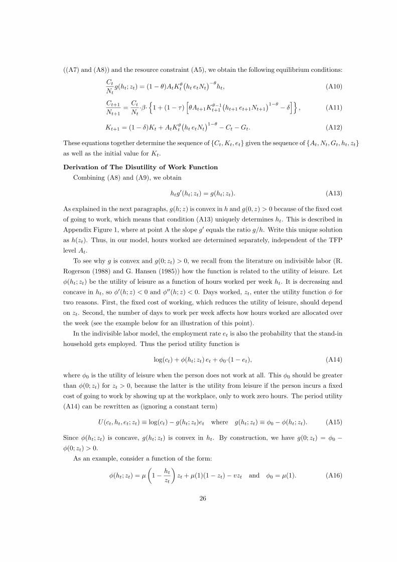
((A7) and (A8)) and the resource constraint (A5), we obtain the following equilibrium conditions:

Ct

Ntg(ht; zt) = (1− θ)AtK

θt

(ht etNt

)−θht, (A10)

Ct+1

Nt+1=Ct

Nt·β·{

1 + (1− τ)[θAt+1K

θ−1t+1

(ht+1 et+1Nt+1

)1−θ − δ]}

, (A11)

Kt+1 = (1− δ)Kt +AtKθt

(ht etNt

)1−θ − Ct −Gt. (A12)

These equations together determine the sequence of {Ct,Kt, et} given the sequence of {At, Nt, Gt, ht, zt}as well as the initial value for Kt.

Derivation of The Disutility of Work Function

Combining (A8) and (A9), we obtain

htg′(ht; zt) = g(ht; zt). (A13)

As explained in the next paragraphs, g(h; z) is convex in h and g(0, z) > 0 because of the fixed cost

of going to work, which means that condition (A13) uniquely determines ht. This is described in

Appendix Figure 1, where at point A the slope g′ equals the ratio g/h. Write this unique solution

as h(zt). Thus, in our model, hours worked are determined separately, independent of the TFP

level At.

To see why g is convex and g(0; zt) > 0, we recall from the literature on indivisible labor (R.

Rogerson (1988) and G. Hansen (1985)) how the function is related to the utility of leisure. Let

φ(ht; zt) be the utility of leisure as a function of hours worked per week ht. It is decreasing and

concave in ht, so φ′(h; z) < 0 and φ′′(h; z) < 0. Days worked, zt, enter the utility function φ for

two reasons. First, the fixed cost of working, which reduces the utility of leisure, should depend

on zt. Second, the number of days to work per week affects how hours worked are allocated over

the week (see the example below for an illustration of this point).

In the indivisible labor model, the employment rate et is also the probability that the stand-in

household gets employed. Thus the period utility function is

log(ct) + φ(ht; zt) et + φ0·(1− et), (A14)

where φ0 is the utility of leisure when the person does not work at all. This φ0 should be greater

than φ(0; zt) for zt > 0, because the latter is the utility from leisure if the person incurs a fixed

cost of going to work by showing up at the workplace, only to work zero hours. The period utility

(A14) can be rewritten as (ignoring a constant term)

U(ct, ht, et; zt) ≡ log(ct)− g(ht; zt)et where g(ht; zt) ≡ φ0 − φ(ht; zt). (A15)

Since φ(ht; zt) is concave, g(ht; zt) is convex in ht. By construction, we have g(0; zt) = φ0 −φ(0; zt) > 0.

As an example, consider a function of the form:

φ(ht; zt) = µ

(1− ht

zt

)zt + µ(1)(1− zt)− vzt and φ0 = µ(1). (A16)

26

Here, µ is the utility of leisure per day (with daily time endowment normalized to unity) as a

function of daily leisure hours and v (> 0) is the fixed cost of commuting per working day. The

g function is

g(ht; zt) =[v + µ(1)− µ

(1− ht

zt

)]zt. (A17)

We have g(0; zt) = −vzt > 0 for zt > 0 as required. It is easy to see that h(z), determined by

(A13), is proportional to z (so hours worked per day, h(z)/z, does not depend on z).

Detrending

We can detrend the model by defining

kt ≡Kt

A1

1−θ

t Nt

, ct ≡Ct

A1

1−θ

t Nt

, yt ≡Yt

A1

1−θ

t Nt

, γt ≡A

11−θ

t+1

A1

1−θ

t

, ψt ≡Gt

Yt, nt ≡

Nt+1

Nt. (A18)

Also define the detrended capital-labor ratio ( KhE deflated by the TFP factor A1/(1−θ)

t ) as

detrended capital-labor ratio: xt ≡kt

eth(zt). (A19)

Then, noting that ht = h(zt), the above three equilibrium conditions (A10)-(A12) become

ct g(h(zt); zt) = (1− θ)h(zt)xθt or xt =

ct

(1− θ) h(zt)g(h(zt);zt)

1θ

, (A20)

ct+1 =ctγtβ ·[1 + (1− τ)

(θxθ−1

t+1 − δ)], (A21)

kt+1 =1

γt nt

{[(1− δ) + (1− ψt)xθ−1

t

]kt − ct

}. (A22)

These three equations determine {xt, ct, kt} given {γt, nt, ψt, zt} and given the function g(h; z)

(which generates ht = h(zt) via (A13)). The employment rate et can be recovered from the

definition of xt by the formula

et =kt

h(zt)xt. (A23)

Detrended output yt can be calculated as

yt = kθt (h(zt) et)

1−θ = ktxθ−1t . (A24)

Steady States

If (x, c, k) are steady-state values of (xt, ct, kt) when (zt, γt, nt, ψt) are constant at (γ, n, ψ, z),

they satisfy

c g(h(z); z) = (1− θ)h(z)xθ, (A25)

1 =1γβ ·[1 + (1− τ)

(θxθ−1 − δ

)], (A26)

k =1γ n

{[(1− δ) + (1− ψ)xθ−1

]k − c

}. (A27)

27

These three steady-state equations can be solved for (x, c, k) as

x =

γβ−1

1−τ + δ

θ

1θ−1

, (A28)

c = (1− θ)xθ h

g(h(z); z), (A29)

k =c

1− δ + (1− ψ)xθ−1 − γn=

(1− θ)xθ

1− δ + (1− ψ)xθ−1 − γn· h(z)g(h(z); z)

. (A30)

So the steady-state value of x, which is pinned down by the Euler equation (A26) alone, is

invariant to the functional form of g(· ; ·). The steady-state value of detrended output y can be

calculated easily as

y = kxθ−1 =(1− θ)x2θ−1

1− δ + (1− ψ)xθ−1 − γn· h(z)g(h(z); z)

. (A31)

In this expression, as in the two expressions preceding it, x is given by (A28) which does not

involve z.

The Level-Down Effect

If the steady-state values (γ, n, ψ, z) of the exogenous variables change, then (x, c, k, y) change.

We say that the level-down effect exists if a reduction in z reduces steady-state output (i.e., if∂ y∂ z > 0). From the expression for y given in (A31) and the fact that x (the steady-state value of

the detrended capital-labor ratio) is independent of z, it is clear that

∂ y

∂ z> 0 ⇔

d(

h(z)g(h(z); z)

)d z

> 0. (A32)

We can check empirically whether this condition for the level-down effect holds, because

the first-order condition for et, (A8), implies that the ratio h(zt)/g(h(zt); zt) should equal the

consumption-wage rate ratio Ct/Nt

wt. Appendix Figure 2 plots the log of Ct/Nt

wtagainst zt (days

worked per week) for 1960-2000. 19 It shows, clearly, that the level-down effect existed all

thorough the post-1960 period, except for 1976-84 when the relationship shifted up with the

number of days worked at around 5.5.

Solution Procedure

Returning to the set of equations (A20)-(A22), we now describe our solution procedure for

determining the sequence of endogenous variables. Substituting (A20) into (A21) and (A22), the

19 The data source for hours worked per week is the same as that for hours worked. That is, both hours workedand days worked are from the Monthly Labor Survey (Maitsuki Kinro Tokei Chousa) for establishments with30 or more employees. Those employees include part-time workers. Monthly figures are converted to weeklyfigures by dividing them by four.

28

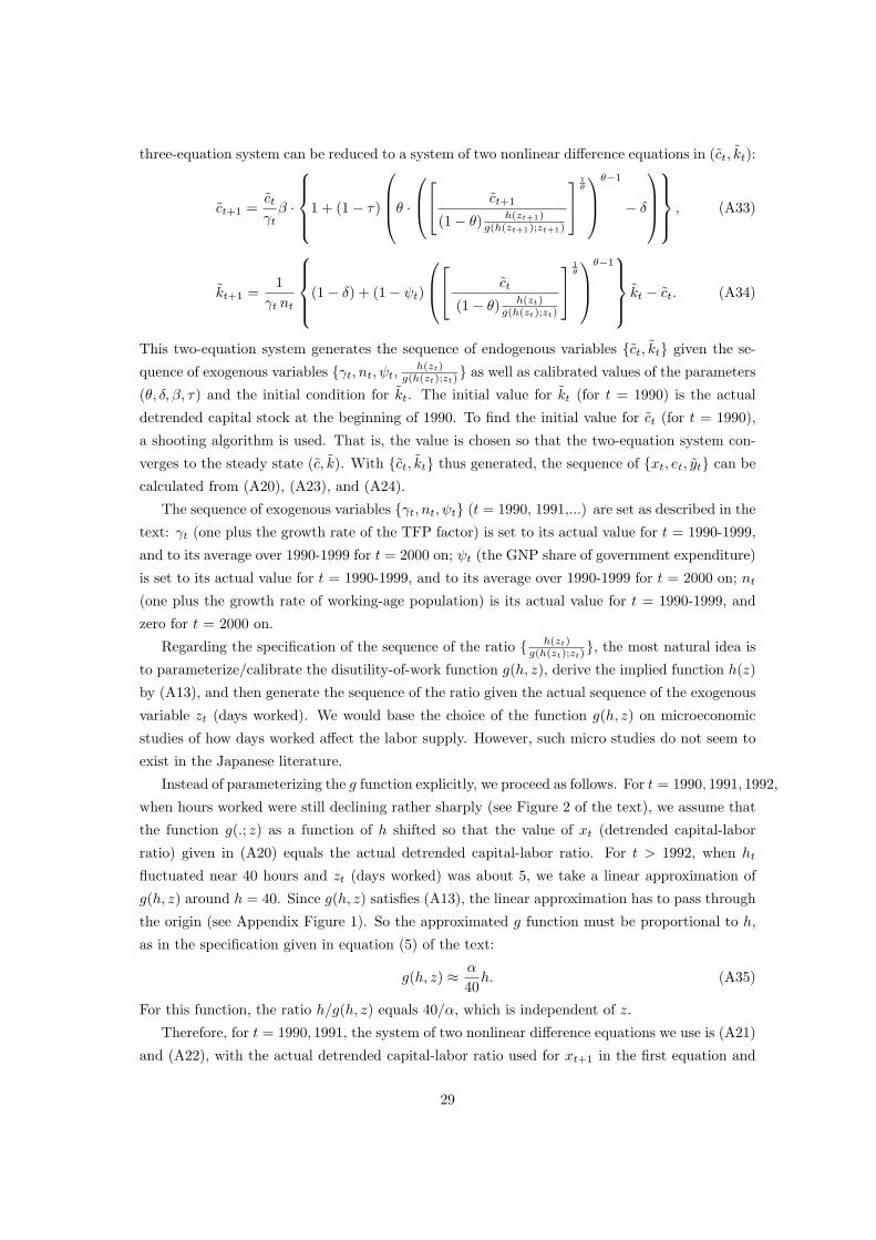
three-equation system can be reduced to a system of two nonlinear difference equations in (ct, kt):

ct+1 =ctγtβ ·

1 + (1− τ)

θ · ct+1

(1− θ) h(zt+1)g(h(zt+1);zt+1)

1θ

θ−1

− δ

, (A33)

kt+1 =1

γt nt

(1− δ) + (1− ψt)

ct

(1− θ) h(zt)g(h(zt);zt)

1θ

θ−1 kt − ct. (A34)

This two-equation system generates the sequence of endogenous variables {ct, kt} given the se-

quence of exogenous variables {γt, nt, ψt,h(zt)

g(h(zt);zt)} as well as calibrated values of the parameters

(θ, δ, β, τ) and the initial condition for kt. The initial value for kt (for t = 1990) is the actual

detrended capital stock at the beginning of 1990. To find the initial value for ct (for t = 1990),

a shooting algorithm is used. That is, the value is chosen so that the two-equation system con-

verges to the steady state (c, k). With {ct, kt} thus generated, the sequence of {xt, et, yt} can be

calculated from (A20), (A23), and (A24).

The sequence of exogenous variables {γt, nt, ψt} (t = 1990, 1991,...) are set as described in the

text: γt (one plus the growth rate of the TFP factor) is set to its actual value for t = 1990-1999,

and to its average over 1990-1999 for t = 2000 on; ψt (the GNP share of government expenditure)

is set to its actual value for t = 1990-1999, and to its average over 1990-1999 for t = 2000 on; nt

(one plus the growth rate of working-age population) is its actual value for t = 1990-1999, and

zero for t = 2000 on.

Regarding the specification of the sequence of the ratio { h(zt)g(h(zt);zt)

}, the most natural idea is

to parameterize/calibrate the disutility-of-work function g(h, z), derive the implied function h(z)

by (A13), and then generate the sequence of the ratio given the actual sequence of the exogenous

variable zt (days worked). We would base the choice of the function g(h, z) on microeconomic

studies of how days worked affect the labor supply. However, such micro studies do not seem to

exist in the Japanese literature.

Instead of parameterizing the g function explicitly, we proceed as follows. For t = 1990, 1991, 1992,

when hours worked were still declining rather sharply (see Figure 2 of the text), we assume that

the function g(.; z) as a function of h shifted so that the value of xt (detrended capital-labor

ratio) given in (A20) equals the actual detrended capital-labor ratio. For t > 1992, when ht

fluctuated near 40 hours and zt (days worked) was about 5, we take a linear approximation of

g(h, z) around h = 40. Since g(h, z) satisfies (A13), the linear approximation has to pass through

the origin (see Appendix Figure 1). So the approximated g function must be proportional to h,

as in the specification given in equation (5) of the text:

g(h, z) ≈ α

40h. (A35)

For this function, the ratio h/g(h, z) equals 40/α, which is independent of z.

Therefore, for t = 1990, 1991, the system of two nonlinear difference equations we use is (A21)

and (A22), with the actual detrended capital-labor ratio used for xt+1 in the first equation and

29

xt in the second equation:

ct+1 =ctγtβ ·[1 + (1− τ)

(θxθ−1

t+1 − δ)], xt = actual detrended capital-labor ratio, (A36)

kt+1 =1

γt nt

[(1− δ) + (1− ψt)xθ−1

t

]kt − ct, xt = actual detrended capital-labor ratio.

(A37)

For t = 1992, the xt+1 in the first equation is very close to 40 hours. So the linear approximation

of g(h, z) is applicable to the first equation, but not to the second. Thus for t = 1992,

ct+1 =ctγtβ ·

1 + (1− τ)

θ ·([ ct+1

(1− θ)(40/α)

] 1θ

)θ−1

− δ

, (A38)

kt+1 =1

γt nt

[(1− δ) + (1− ψt)xθ−1

t

]kt − ct, xt = actual detrended capital-labor ratio.

(A39)

For t > 1992, the system becomes

ct+1 =ctγtβ ·

1 + (1− τ)

θ ·([ ct+1

(1− θ)(40/α)

] 1θ

)θ−1

− δ

, (A40)

kt+1 =1

γt nt

(1− δ) + (1− ψt)

([ct

(1− θ)(40/α)

] 1θ

)θ−1 kt − ct. (A41)

Thus, our solution method for determining the sequence of endogenous variables does not require

data on zt and ht.

To implement this solution procedure, the parameters (θ, δ, β, τ, α) need to be calibrated.

The calibrated values are the same as in the text: θ = 0.362, δ = 0.089, β = 0.976, τ = 0.480,

α = 1.373. Appendix Figures 3-5 report the simulation obtained from this solution procedure

along with the data and the simulation of the text.

Relation to the Simulation of the Text

The solution procedure underlying the model prediction in the text uses (A40) and (A41) for

all years t = 1990, 1991, ..., which amounts to assuming no level-down effect. 20 This explains

why the decline in GNP is less steep in the text’s simulation than in the simulation just described

above.

20 This is related to the point made by Aoki, Ichiba, and Ktiahara (“A Comment: Workweek Length in Hayashi-Prescott (2002) Model”, November 2002) that the model depends on h and e only through the product h · eif the parameterization of the g function is as given in equation (5) of the text.

30

References

Bayoumi, T. (1999), “The Morning After: Explaining the Slowdown in Japanese Growth in the

1990s,” Journal of International Economics; 53, April 2001, 241-59.

Bernanke, B. and C. Lown (1991), “The Credit Crunch, ” BPEA, 205-239.

Hansen, G., D. (1985), “Indivisible Labor and the Business Cycle,” Journal of Monetary Eco-

nomics, 16, 309-27.

Hayashi, F. (1997), Understanding Savings: Evidence from the United States and Japan, Cam-

bridge: MIT Press.

Hoshi, T. and A. Kashyap (1999), “The Japanese Banking Crisis: Where Did It Come From and

How Will It End?” NBER Macro Annual, 129-201.

Kashyap, A. and J. Stein (1994), “Monetary Policy and Bank Lending,” in G. Mankiw, ed., Mon-

etary Policy. Studies in Business Cycles, vol. 29. Chicago and London: University of Chicago

Press, 1994, 221-56.

Kwon, E. (1998), “Monetary Policy, Land Prices, and Collateral Effects on Economic Fluctua-

tions: Evidence from Japan,” Jour. of Japanese and International Economies, 12, 175-203.

Motonishi, T. and H. Yoshikawa (1999), “Causes of the Long Stagnation of Japan during the

1990s, ” Jour. of Japanese and International Economies, 181-200.

Ogawa, K. and K. Suzuki (1998), “Land Value and Corporate Investment: Evidence from Japanese

Panel Data, ” Jour. of Japanese and International Economies, 232-249.

Ogawa, K. and S. Kitasaka (1998), Asset Markets and Business Cycles (in Japanese), Nihon Keizai

Shinbunsha.

Peck, M. J., R. C. Levin, and A. Goto (1988), “Picking Losers: Public Policy Toward Declining

Industries in Japan,” in Government Policy Towards Industry in the United States and Japan, J.

B. Shoven, ed., Cambridge: Cambridge University Press, 165-239.

Rogerson, R. (1988), “Indivisible Labor, Lotteries and Equilibrium,” Journal of Monetary Eco-

nomics, 21, 3-16.

Sasaki, Y. (2000), “Prudential Policy for Private Financial Institutions,” mimeo, Japanese Postal

Savings Research Institute.

Woo, D. (1999), “In Search of ‘Capital Crunch’: Supply Factors behind the Credit Slowdown in

Japan,” IMF Working Paper No. 99/3.

31

Table I: Accounting for Japanese Growth per Person Aged 20-69

Period Growth rate FactorsTFPfactor

Capitalintensity

Workweeklength

Employmentrate

1960-1973 7.2% 6.5% 2.3% -0.8% -0.7%1973-1983 2.2% 0.8% 2.1% -0.4% -0.3%1983-1991 3.6% 3.7% 0.2% -0.5% 0.1%1991-2000 0.5% 0.3% 1.4% -0.9% -0.4%

Table II: Calibration

Parameter Valueθ 0.362δ 0.089β 0.976α 1.373τ 0.480

Table III: Sources of Investment Finance for Nonfinancial Corporations

Sources of fund as fraction of investment 1984-1988 1993-1999(a) Bank loans 52.2% -4.8%(b) Sale of land -6.9% 5.7%(c) Gross savings 79.2% 88.1%(d) Net increase in other liabilities -24.5% 11.0%Total 100% 100%

Table IV: Sources of Investment Finance for Small Nonfinancial Corporations

Sources of fund as fraction of investment Fiscal year 1984-88 Fiscal year 1993-2000(a) Bank loans 64.5% -12.6%(b) Sale of land -18.3% -20.8%(c) + (d) other 53.8% 133.4%Total 100% 100%

32

Table V: Cross-Section Regression of GDP Growth on Loan Growth

Regression 1 Regression 2Recession years Independent variable is

loan growth to all firmsfrom March to March overindicated years

Independent variable isloan growth to small firmsfrom March to March overindicated years

1979 – 1982 0.046 (0.3) 0.125 (0.9)1990 - 1993 0.090 (1.0) 0.049 (0.6)1996 - 1998 0.125 (2.0) 0.120 (1.7)Note: t values in parentheses. The dependent variable is GDP growth rateover indicated fiscal years. The coefficient on the constant in the regression isnot reported.

33

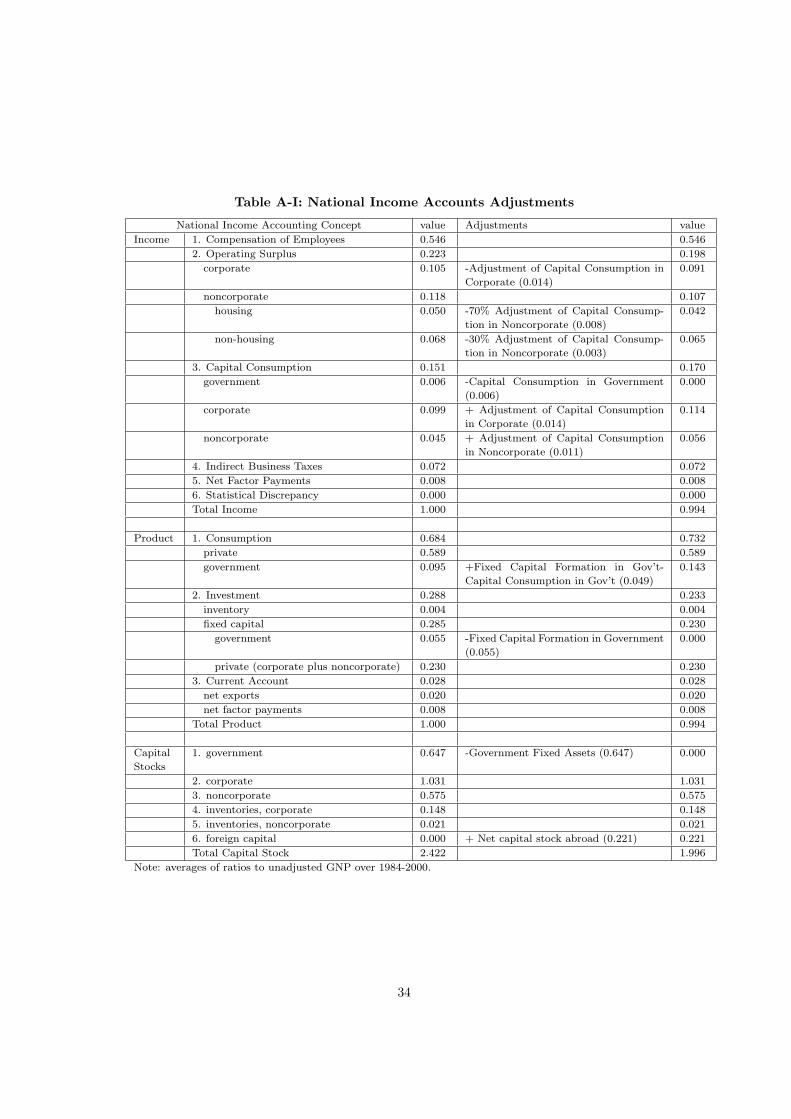
Table A-I: National Income Accounts Adjustments

National Income Accounting Concept value Adjustments value

Income 1. Compensation of Employees 0.546 0.546

2. Operating Surplus 0.223 0.198

corporate 0.105 -Adjustment of Capital Consumption in

Corporate (0.014)

0.091

noncorporate 0.118 0.107

housing 0.050 -70% Adjustment of Capital Consump-

tion in Noncorporate (0.008)

0.042

non-housing 0.068 -30% Adjustment of Capital Consump-

tion in Noncorporate (0.003)

0.065

3. Capital Consumption 0.151 0.170

government 0.006 -Capital Consumption in Government

(0.006)

0.000

corporate 0.099 + Adjustment of Capital Consumption

in Corporate (0.014)

0.114

noncorporate 0.045 + Adjustment of Capital Consumption

in Noncorporate (0.011)

0.056

4. Indirect Business Taxes 0.072 0.072

5. Net Factor Payments 0.008 0.008

6. Statistical Discrepancy 0.000 0.000

Total Income 1.000 0.994

Product 1. Consumption 0.684 0.732

private 0.589 0.589

government 0.095 +Fixed Capital Formation in Gov’t-

Capital Consumption in Gov’t (0.049)

0.143

2. Investment 0.288 0.233

inventory 0.004 0.004

fixed capital 0.285 0.230

government 0.055 -Fixed Capital Formation in Government

(0.055)

0.000

private (corporate plus noncorporate) 0.230 0.230

3. Current Account 0.028 0.028

net exports 0.020 0.020

net factor payments 0.008 0.008

Total Product 1.000 0.994

Capital

Stocks

1. government 0.647 -Government Fixed Assets (0.647) 0.000

2. corporate 1.031 1.031

3. noncorporate 0.575 0.575

4. inventories, corporate 0.148 0.148

5. inventories, noncorporate 0.021 0.021

6. foreign capital 0.000 + Net capital stock abroad (0.221) 0.221

Total Capital Stock 2.422 1.996

Note: averages of ratios to unadjusted GNP over 1984-2000.

34

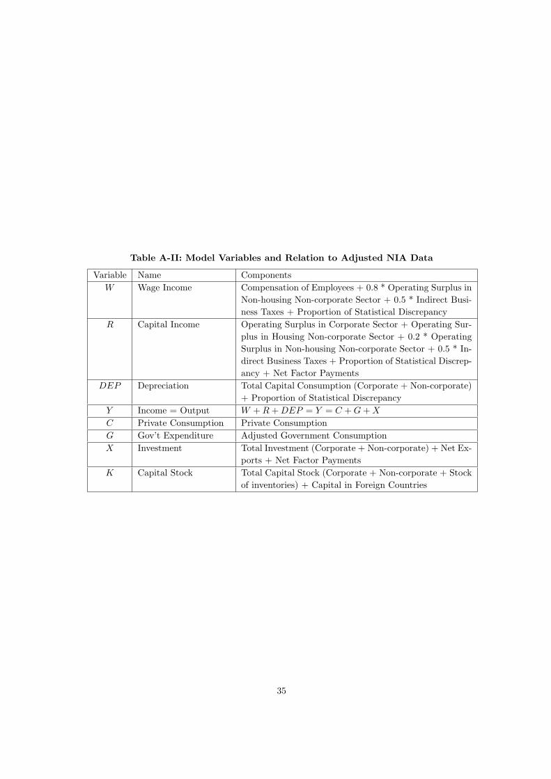
Table A-II: Model Variables and Relation to Adjusted NIA Data

Variable Name ComponentsW Wage Income Compensation of Employees + 0.8 * Operating Surplus in

Non-housing Non-corporate Sector + 0.5 * Indirect Busi-ness Taxes + Proportion of Statistical Discrepancy

R Capital Income Operating Surplus in Corporate Sector + Operating Sur-plus in Housing Non-corporate Sector + 0.2 * OperatingSurplus in Non-housing Non-corporate Sector + 0.5 * In-direct Business Taxes + Proportion of Statistical Discrep-ancy + Net Factor Payments

DEP Depreciation Total Capital Consumption (Corporate + Non-corporate)+ Proportion of Statistical Discrepancy

Y Income = Output W +R+DEP = Y = C +G+X

C Private Consumption Private ConsumptionG Gov’t Expenditure Adjusted Government ConsumptionX Investment Total Investment (Corporate + Non-corporate) + Net Ex-

ports + Net Factor PaymentsK Capital Stock Total Capital Stock (Corporate + Non-corporate + Stock

of inventories) + Capital in Foreign Countries

35

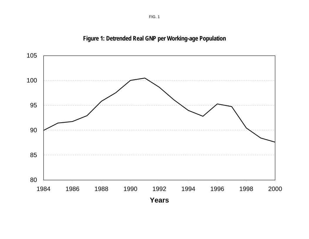
FIG. 1

Figure 1: Detrended Real GNP per Working-age Population

80

85

90

95

100

105

1984 1986 1988 1990 1992 1994 1996 1998 2000

Years

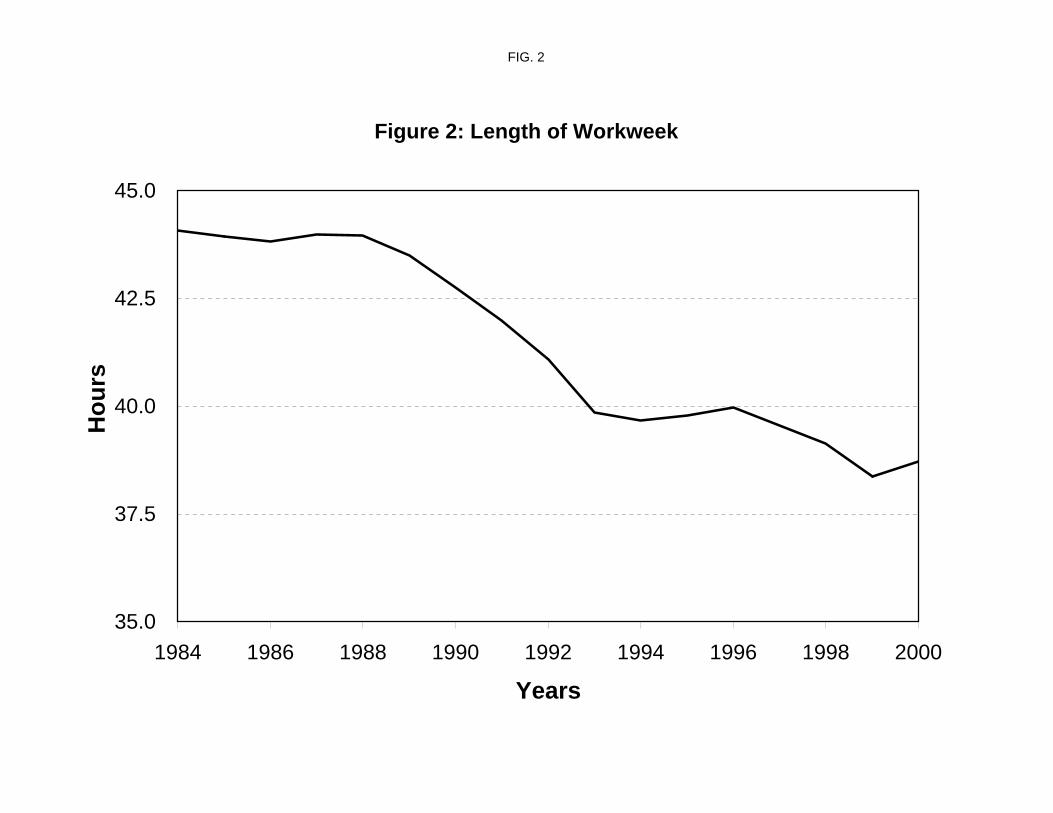
FIG. 2

Figure 2: Length of Workweek

35.0

37.5

40.0

42.5

45.0

1984 1986 1988 1990 1992 1994 1996 1998 2000

Years

Hou

rs

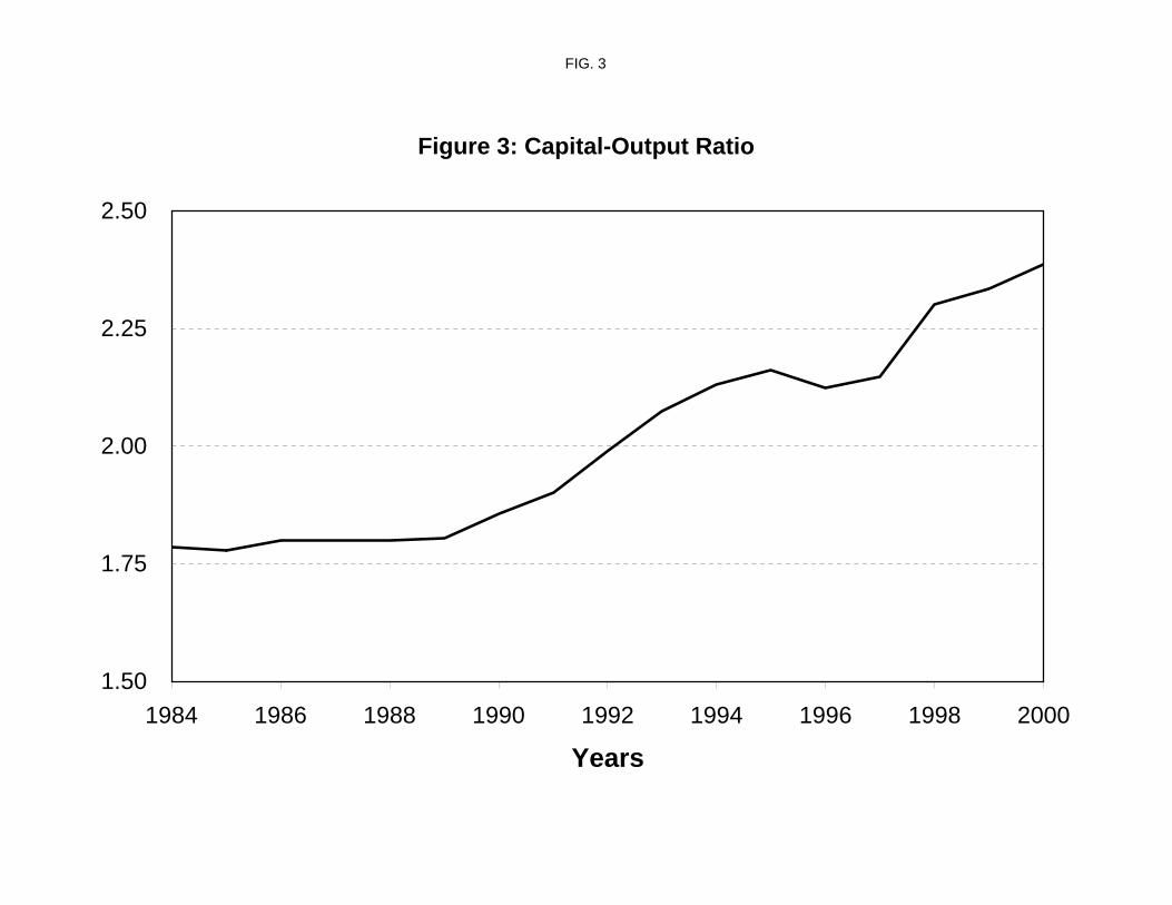
FIG. 3

Figure 3: Capital-Output Ratio

1.50

1.75

2.00

2.25

2.50

1984 1986 1988 1990 1992 1994 1996 1998 2000

Years

FIG. 4

Figure 4: After-tax Rate of Return

3%

4%

5%

6%

7%

1984 1986 1988 1990 1992 1994 1996 1998 2000

Years

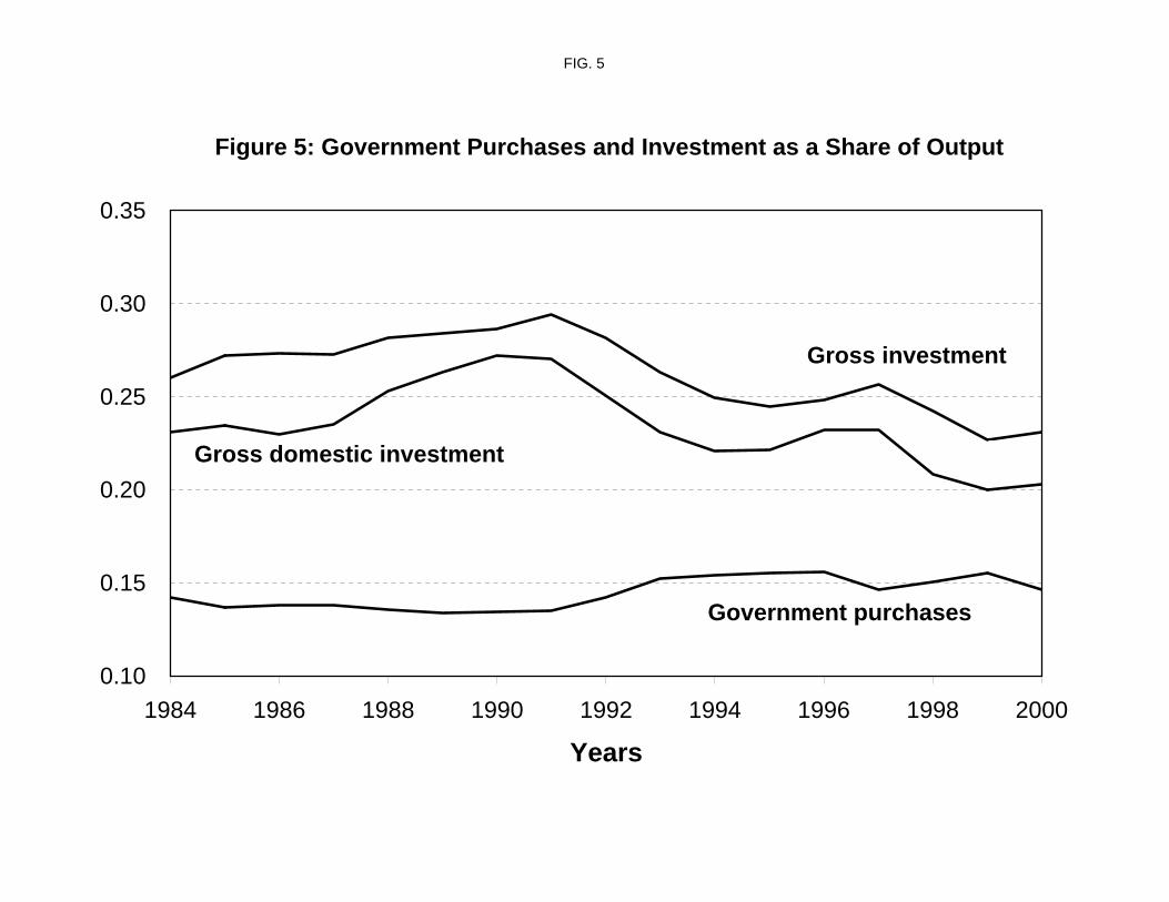
FIG. 5

Figure 5: Government Purchases and Investment as a Share of Output

0.10

0.15

0.20

0.25

0.30

0.35

1984 1986 1988 1990 1992 1994 1996 1998 2000

Years

Gross domestic investment

Gross investment

Government purchases

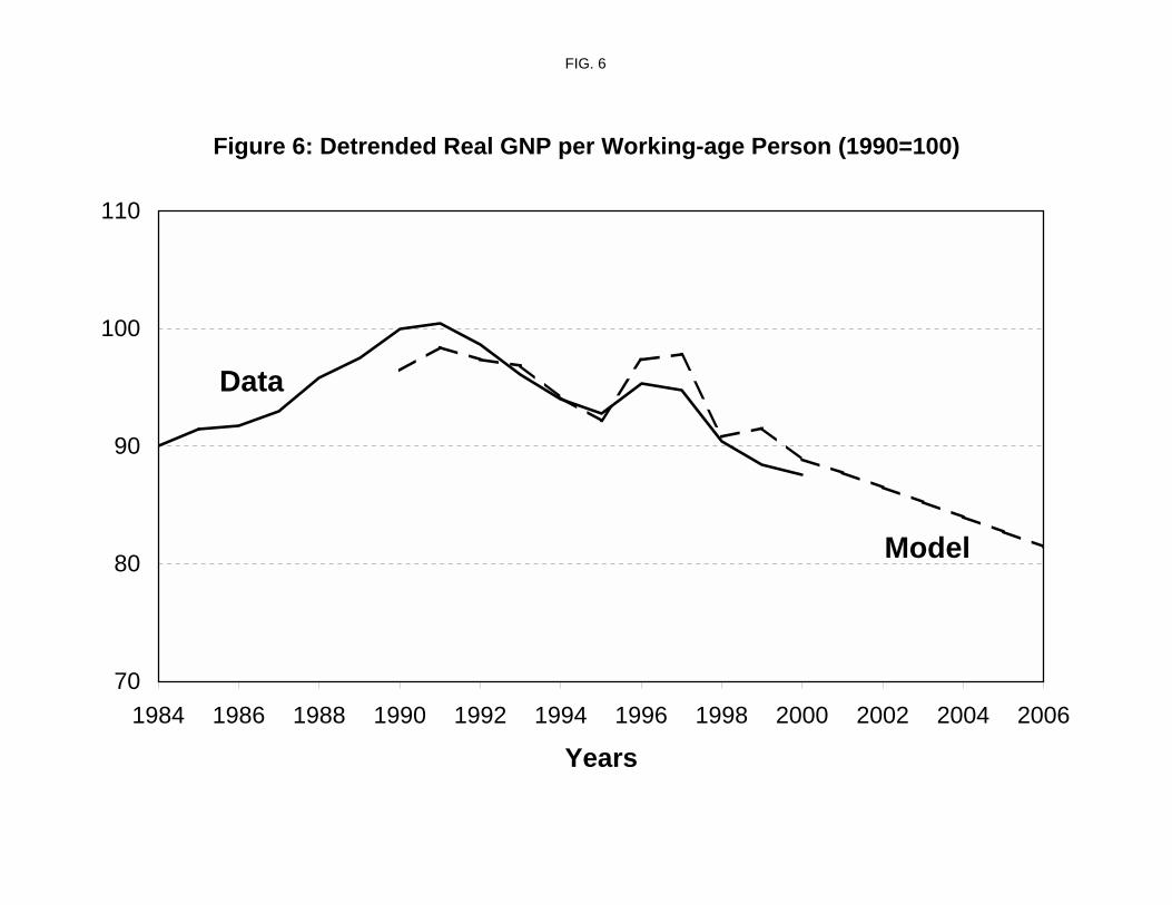
FIG. 6

Figure 6: Detrended Real GNP per Working-age Person (1990=100)

70

80

90

100

110

1984 1986 1988 1990 1992 1994 1996 1998 2000 2002 2004 2006

Years

Data

Model

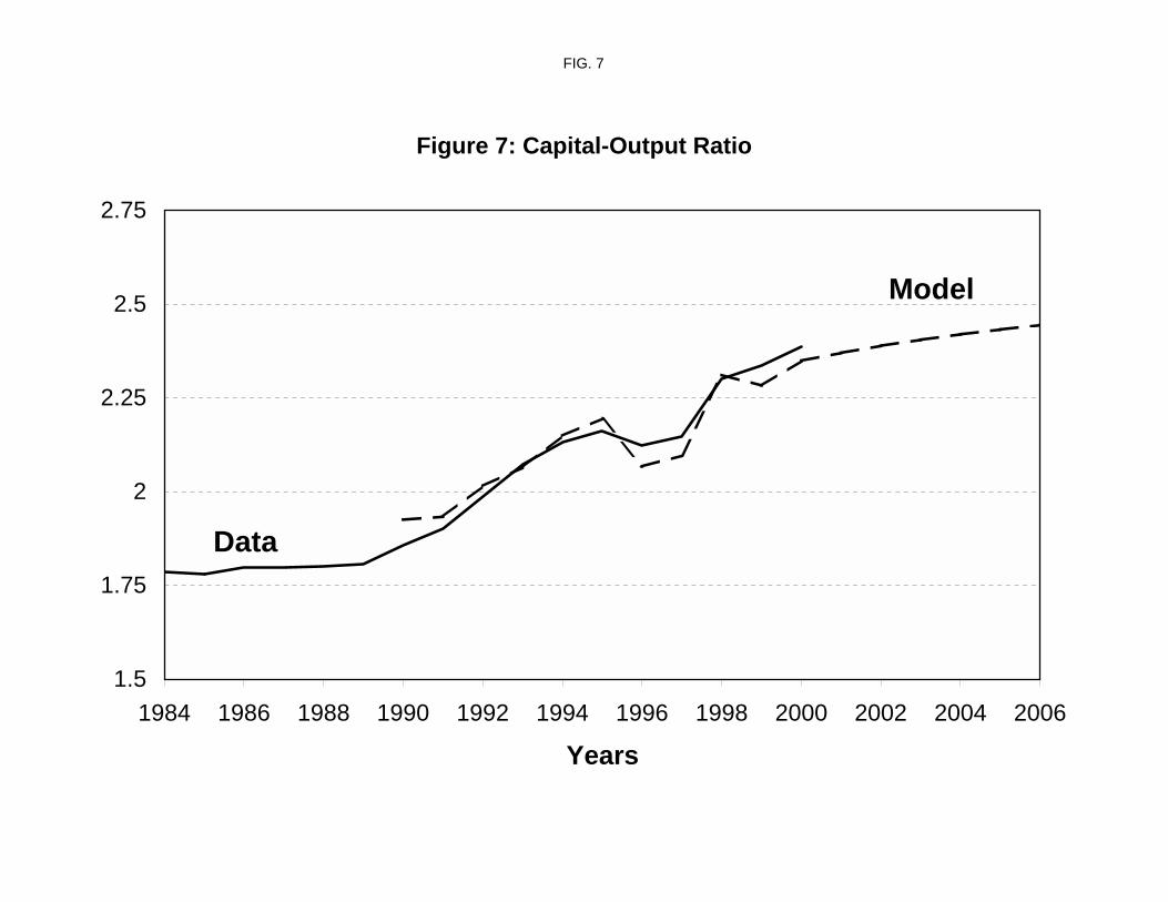
FIG. 7

Figure 7: Capital-Output Ratio

1.5

1.75

2

2.25

2.5

2.75

1984 1986 1988 1990 1992 1994 1996 1998 2000 2002 2004 2006

Years

Data

Model

FIG. 8

Figure 8: After-tax Rate of Return

2%

3%

4%

5%

6%

7%

8%

1984 1986 1988 1990 1992 1994 1996 1998 2000 2002 2004 2006

Years

Data

Model

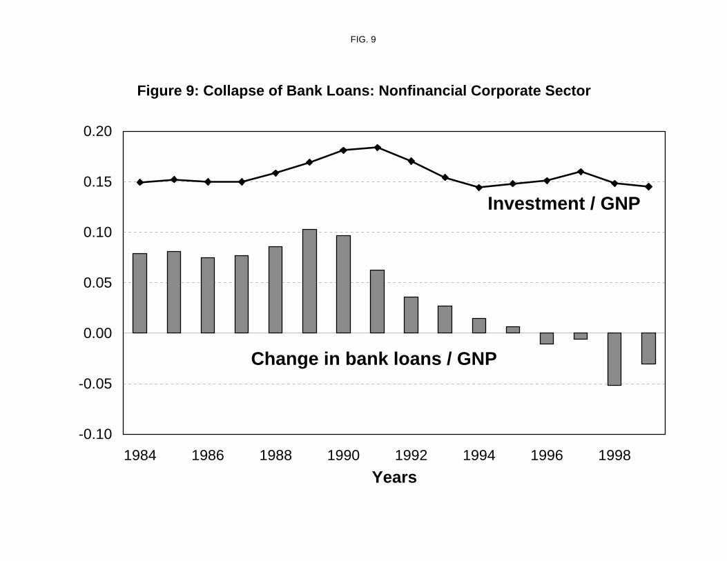
FIG. 9

Figure 9: Collapse of Bank Loans: Nonfinancial Corporate Sector

-0.10

-0.05

0.00

0.05

0.10

0.15

0.20

1984 1986 1988 1990 1992 1994 1996 1998Years

Change in bank loans / GNP

Investment / GNP

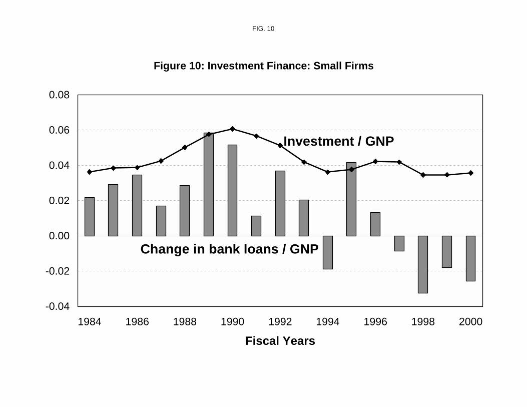
FIG. 10

Figure 10: Investment Finance: Small Firms

-0.04

-0.02

0.00

0.02

0.04

0.06

0.08

1984 1986 1988 1990 1992 1994 1996 1998 2000

Fiscal Years

Change in bank loans / GNP

Investment / GNP

FIG. 11

Figure 11: Ratio fo Cash plus Deposits to Capital Stock: Small Firms

0.00

0.10

0.20

0.30

0.40

0.50

0.60

0.70

0.80

1984.2 1986.2 1988.2 1990.2 1992.2 1994.2 1996.2 1998.2 2000.2

Quarters

Appendix Figure 1

h 0 h(z)

A

g(h; z)

g/h

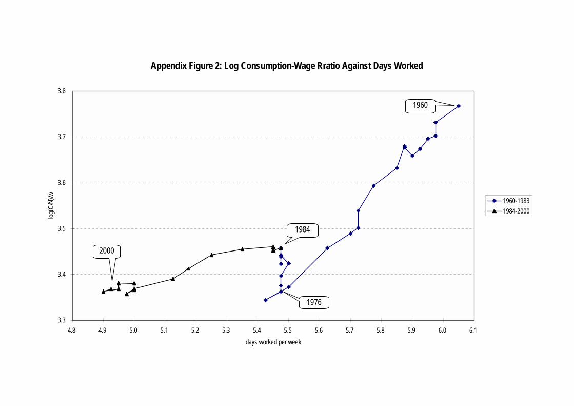
Appendix Figure 2: Log Consumption-Wage Rratio Against Days Worked

3.3

3.4

3.5

3.6

3.7

3.8

4.8 4.9 5.0 5.1 5.2 5.3 5.4 5.5 5.6 5.7 5.8 5.9 6.0 6.1days worked per week

log(C

/N)/w 1960-1983

1984-2000

1976

1960

1984

2000

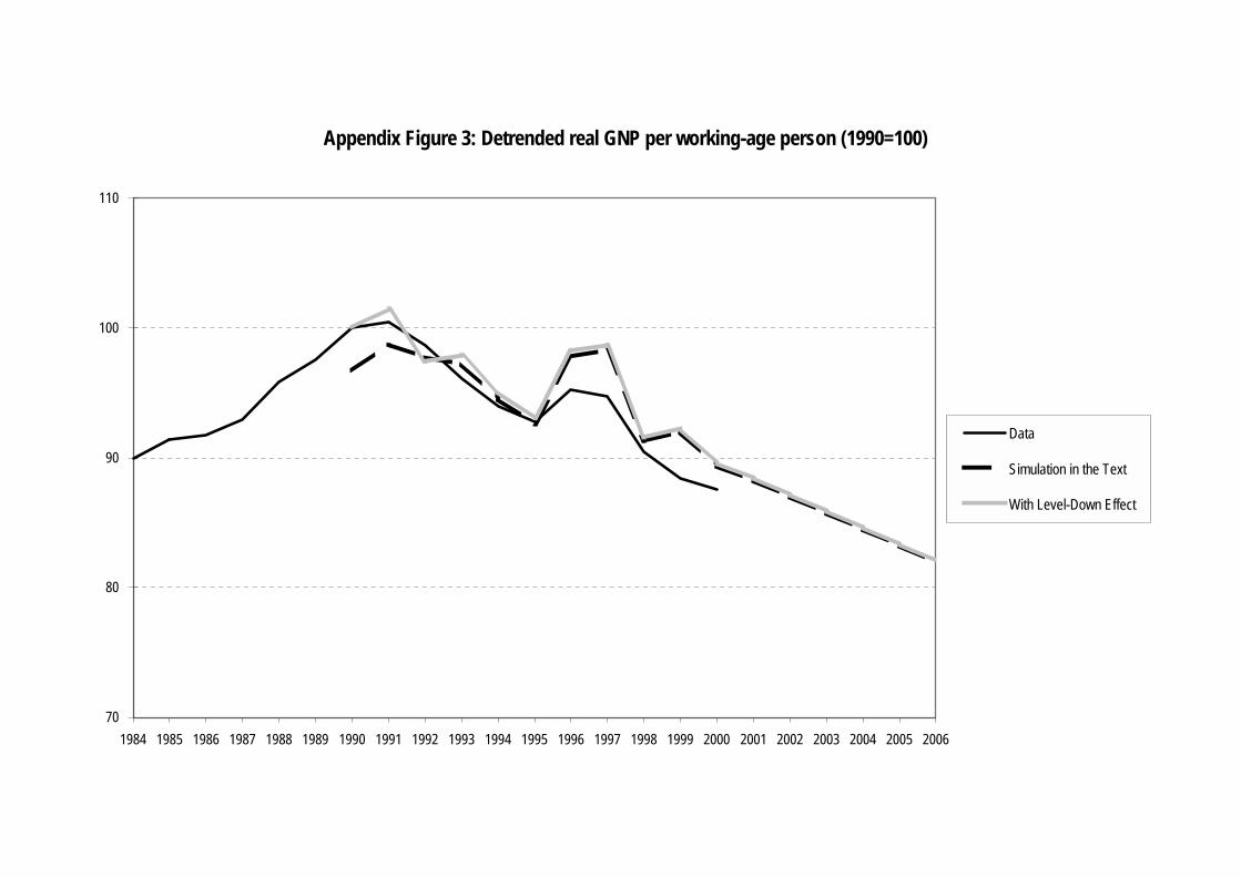
Appendix Figure 3: Detrended real GNP per working-age person (1990=100)

70

80

90

100

110

1984 1985 1986 1987 1988 1989 1990 1991 1992 1993 1994 1995 1996 1997 1998 1999 2000 2001 2002 2003 2004 2005 2006

Data

Simulation in the Text

With Level-Down Effect

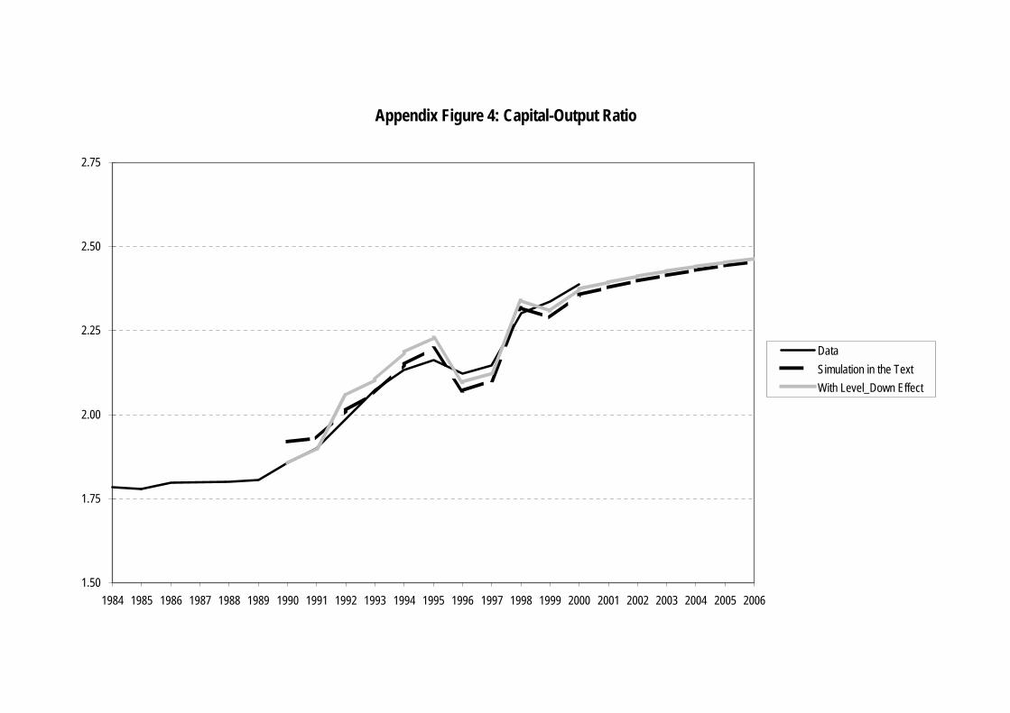
Appendix Figure 4: Capital-Output Ratio

1.50

1.75

2.00

2.25

2.50

2.75

1984 1985 1986 1987 1988 1989 1990 1991 1992 1993 1994 1995 1996 1997 1998 1999 2000 2001 2002 2003 2004 2005 2006

DataSimulation in the TextWith Level_Down Effect

Appendix Figure 5: After-tax rate of return

2%

3%

4%

5%

6%

7%

8%

1984 1985 1986 1987 1988 1989 1990 1991 1992 1993 1994 1995 1996 1997 1998 1999 2000 2001 2002 2003 2004 2005 2006

DataSimulation in the TextWith Level-Down Effect