THE 2021 SSP SCENARIOS OF THE IMAGE 3.2 MODEL

Detlef Van Vuuren, Elke Stehfest, David Gernaat et al.

Oktober 2021

Colophon

THE 2021 SSP SCENARIOS OF THE IMAGE 3.2 MODEL © PBL Netherlands Environmental Assessment Agency The Hague, 2021 PBL publication number: 4740 https://doi.org/10.31223/X5CG92

Corresponding author Detlef.vanvuuren@pbl.nl

Author(s) Detlef Van Vuuren, Elke Stehfest, David Gernaat, Harmen Sytze De Boer, Vassilis Daioglou1, Jonathan Doelman, Oreane Edelenbosch1, Mathijs Harmsen, Willem-Jan van Zeist2, Maarten van den Berg, Ioannis Dafnomilis, Mariesse van Sluisveld, Andrzej Tabeau2, Lotte de Vos, Liesbeth de Waal, Nicole van den Berg1, Arthur Beusen, Astrid Bos, Hester Biemans3, Lex Bouwman, Hsing-Hsuan Chen, Sebastiaan Deetman1,4, Anteneh Dagnachew, Andries Hof, Hans van Meijl2, Johan Meyer, Stratos Mikropoulos1, Mark Roelfsema, Aafke Schipper15, Heleen van Soest, Isabela Tagomori, Victhalia Zapata1

1 Copernicus Institute of Sustainable Development Utrecht University, the Netherlands; 2 Wageningen Economic Research, The Hague, the Netherlands; 3 Environmental Research (Alterra), Wageningen University & Research, Wageningen, The Netherlands; 4 Centrum voor Milieuwetenschappen (CML) - Universiteit Leiden, the Netherlandsl; 5 Environmental Science, Radboud Universiteit, the Netherlands

Production coordination PBL Publishers Parts of this publication may be reproduced, providing the source is stated, in the form: Van Vuuren et al. (2021), the 2021 SSP scenarios of the IMAGE 3.2 model. The Hague: PBL Netherlands Environmental Assessment Agency. PBL Netherlands Environmental Assessment Agency is the national institute for strategic policy analysis in the fields of the environment, nature and spatial planning. We contribute to improving the quality of political and administrative decision-making by conducting outlook studies, analyses and evaluations in which an integrated approach is considered paramount. Policy relevance is the prime concern in all of our studies. We conduct solicited and unsolicited research that is both independent and scientifically sound.

PBL | 3

Contents Summary 4

1 Introduction 6

2 Methods 7 2.1 Overall model description 7 2.2 Recent model updates 8 2.3 Scenario assumptions 9

3 Results 12 3.1 Energy system 12 3.2 Food systems and land use 13 3.3 Greenhouse gas emissions 15 3.4 Climate policy strategies 16

4 Conclusions 18

References 19

Appendix A: Assumptions for baselines 21

PBL | 4

Summary The SSP (Shared Socio-economic Pathways) scenarios are intensively used in climate and environmental research to explore uncertain future developments and possible response strategies. This paper briefly describes an update of the SSP scenarios generated by the IMAGE 3.2 model. The paper presents the changes in method and key scenario updates. As such, it serves as a key reference for the updated SSP scenarios with IMAGE 3.2.

PBL | 5

PBL | 6

1 Introduction Model-based scenarios are intensively used in climate and environmental research to explore uncertain future developments and possible response strategies. Among the most used scenarios are the Representative Concentration Pathways (RCPs) [1] and the Shared Socio-economic Pathways (SSPs) [2-4]. The RCPs, published in 2011, explored a wide range of emission pathways, while the SSPs presented a much more comprehensive set of scenarios covering narratives, elaboration of scenario drivers and quantification of energy, land-use and emission trends. Both played a critical role in recent IPCC assessments [5, 6] and have also been widely used in other research fields. For instance, they formed an input to IPBES and the Global Land Outlook [7], and at the moment, several thousand papers have used the SSPs [8]. The elaboration of the SSPs, published in 2017, was based on six different integrated assessment models (IAMs) [2]. The IMAGE model was among these, focusing mostly on SSP1 and elaborating scenarios for SSP2, SSP3, the associated mitigation cases [9], and later also SSP4 and SSP5 variants. Since 2017, the world has changed a lot. Some of the recent trends might also have long-term consequences. Moreover, while the SSPs are mostly meant to explore long-term developments, they are often also used as references for assessments on climate policy in 2030 or 2050. In this context, it is important to update the scenarios regularly. Critical issues include the developments regarding the COVID-19 pandemic, the cost reductions and capacity developments of renewable energy, and the expectations regarding electric vehicles. Other updates also include insights into the actual development of demographic, economic, energy and land-use trends over the 2010-2020 period. Finally, in the past few years, the IMAGE model itself has been developed further, including, for instance, more details regarding crop types and industrial energy use. In this context, the IMAGE SSP scenario set has been updated. This paper briefly describes these updates, presents some key results, and serves as a key reference for the updated SSP scenarios with IMAGE 3.2.

PBL | 7

2 Methods

2.1 Overall model description IMAGE is an integrated assessment model framework that simulates global and regional environmental consequences of changes in human activities (see also www.pbl.nl/IMAGE). Detailed model documentation is available online1. IMAGE includes a detailed description of the energy and land-use system. It simulates most of the socio-economic parameters for 26 regions and most environmental parameters, depending on the variable, based on a geographical grid of 30 by 30 min or 5 by 5 min (respectively around 50 km and 10 km at the equator). The model has been designed to analyse large-scale and long-term interactions between human development and the natural environment and identify response strategies to global environmental change based on assessing options for mitigation and adaptation. IMAGE is a framework with a modular structure, with some components operating together in a hard-coupled mode and others connected through soft links (where models run independently with information exchange via data files). The IMAGE framework is structured around the causal chain of key global sustainability issues and comprises two main systems: 1) the human or socio-economic system that describes the long-term development of human activities relevant for sustainable development; and 2) the earth system that describes changes in natural systems, such as the carbon and hydrological cycle and climate. The two systems are linked through emissions, land use, climate feedbacks and potential human policy responses. Important inputs to the model are descriptions of the future development of so-called direct and indirect drivers of global environmental change: Exogenous assumptions on population, economic development, lifestyle, policies and technology change form a key input into the energy system model TIMER and the food and agriculture system model MAGNET [10]. TIMER is a system-dynamics energy system simulation model describing key trends in energy use and supply; changes in model variables are calculated based on information from the previous time step. MAGNET is a computable general equilibrium (CGE) model [10]; it uses information from IMAGE on land availability, suitability, and changes in crop yields due to climate change and agricultural expansion into heterogeneous land areas. Together with the drivers described above, regional consumption, production and trade in agricultural commodities is computed. The results from MAGNET on production and endogenous yield changes are used in IMAGE to calculate spatially explicit land-use change and the environmental impacts on carbon, nutrient and water cycles, biodiversity, and climate. In IMAGE, the main interaction with the Earth system is by changes in energy, food and biofuel production that induce land-use changes and emissions of carbon dioxide and other greenhouse gases. A key component of the earth system is the LPJmL model [11] that is hard-coupled to IMAGE (see also [12] for details). LPJmL covers the terrestrial carbon cycle and vegetation dynamics. This model is used to determine productivity at the grid cell level for natural and cultivated ecosystems based on plant and crop functional types. Based on the regional production levels and the output of LPJmL, a set of allocation rules in IMAGE determine the actual land cover. A key dynamic is the expansion of agricultural land, which follows empirically-based statistical

1 https://models.pbl.nl/image/index.php/Welcome_to_IMAGE_3.0_Documentation .

PBL | 8

suitability layers derived from ESA-CCI land-use change data [13]. The calculated emissions of greenhouse gases and air pollutants are used in IMAGE to derive changes in concentrations of greenhouse gases, ozone precursors and species involved in aerosol formation on a global scale. Climatic change is calculated as global mean temperature change using a slightly adapted version of the MAGICC 6.0 climate model [14]. The changes in temperature and precipitation in each grid cell are derived from the global mean temperature using a pattern-scaling approach. The model accounts for several feedback mechanisms between climate change and dynamics in the energy, land and vegetation systems.

2.2 Recent model updates In 2014, the IMAGE-3 model was finalised [15]. In 2020, we finalised the IMAGE 3.2 model. The IMAGE 3.2 model goes beyond the earlier model versions in several ways:

• The model has been fully calibrated up to 2015, and where possible, even to a more recent date (2018 for energy system variables, 2020 for renewables capacity and CO2 emission data). Moreover, the base year for scenario analysis was set at 2020, implying that scenarios follow the same trajectory in the 2015-2020 period.

• The detail in modelling energy demand was further improved. This relates to improvements in the end-use sectors transport, industry, buildings, services and agriculture.

• In transport, the technology costs of electric and hydrogen-fuelled transport technologies were updated. Moreover, an explicit representation of energy use of gas pipelines was added and calibrated to IEA data. Finally, also a new CNG fuelled car type was added.

• For buildings, an explicit representation of insulation levels and renovations for the housing stock was added. In addition, heat pumps were added as an additional heating technology [16].

• For the service sector, the model now also has a description of the specific energy services. • The industry model has been split into a steel, cement, food processing, paper and pulp,

chemicals and non-energy and other industry sectoral definition. All sectors contain disaggregated technology descriptions. Ammonia demand (as part of chemicals) has been linked to agricultural production.

• In energy conversion, details were added to electricity representation and hydrogen production (using a residual load duration curve approach) [17]. The data on existing plants was updated. In addition, hydropower modelling was made dynamic (instead of a prescribed fraction of total potential) using the information on potential and cost via cost curves. Also, an improved technological learning formulation was introduced. Finally, rooftop PV was added as an additional form of PV power supply.

• The modelling of bio-energy was greatly improved, using dynamic land-use change emission factors based on the IMAGE land model [18] and adding biofuel production with carbon capture and storage technology routes [19]. Moreover, a BECCS option was added to liquid biofuel production

• The data on fossil fuel reserves and resources was updated. • Climate impacts on different forms of renewable energy (solar, wind, hydropower and bio-

energy) were added to the model [20]. • In land use, the number of crop categories was increased to 16 representing all crop

production reported by the FAO: wheat, rice, maise, tropical cereals, other temperate

PBL | 9

cereals, pulses, soybeans, temperate oil crops, tropical oil crops, temperate roots & tubers, tropical roots & tubers, sugar crops, oil palm, vegetables & fruits, other non-food, luxury crops, spices, plant-based fibres).

• Deforestation due to other reasons than agricultural expansion was improved based on FAO data in combination with satellite data from ESA-CCI.

• Anthropogenic land use for other reasons than agriculture or built-up is accounted for. • The link between the agriculture-economic model MAGNET and the IMAGE model was

significantly improved concerning climate change effects and exogenous and endogenous trends in crop yield changes [21].

• The modelling of land-based mitigation in IMAGE and MAGNET was improved, including avoided deforestation and afforestation through MAC curves in FAIR [22] and accounting for the interaction non-CO2 mitigation and the agriculture and food system [23].

• Greenhouse gas emissions from peatland degradation were included. • The water modelling in IMAGE linked to LPJmL was improved, introducing municipal,

energy and industry water demand in LPJmL and making it possible to account for environmental flow requirements [24].

• All non-CO2 GHG marginal abatement cost curves were updated based on recent literature.[25]

2.3 Scenario assumptions The SSP framework defines five storylines that strongly differ in the challenges for mitigation and adaptation. Each of the scenarios is elaborated first-of-all in terms of a reference scenario (i.e. in the absence of climate policy). In the case of SSP1-SSP2, these reference scenarios function as a basis for subsequent analysis of the impact of climate policy, implemented in the framework as policies aiming to achieve forcing levels consistent with the Representative Concentration Pathways. The SSP1 scenario depicts a world that aims for green growth (sustainable development). For instance, the assumed rapid technology development and concerns about environmental impacts lead to high energy efficiency and high shares of renewable energy. The investments into education and development at the same time are assumed to lead to low population levels and, as a result, relatively low pressure on land. The SSP2 scenario indicates possible development under median assumptions. The SSP3 scenario describes a world of fragmentation. Consequently, economic growth and technology development are assumed to be slow. SSP4 describes a strong divergence between high and low-income groups (inequality), while, finally, SSP5 describes a rapid growth scenario based on the use of fossil fuels.

PBL | 10

Figure 1: GDP and population trajectories for all SSPs (panel a and panel b). Data is presented in 5-year steps (as a result, the COVID-19 crisis is not clearly visible). The lower panel presents the annual data for SSP2 in the IMAGE 3.0 (red) and IMAGE3.2 scenarios (black).

In the elaboration, we use the population projections originally provided for the SSPs. However, we updated the population data based on historical data up to 2020 based on UN data and subsequently used the relative growth of the original projections [26]. For income, we used available data up to 2020, including the impact of Covid-19 and the short-term projections for the 2021-2025 period from IMF [27]. From 2025, the original growth rates of the SSPs were used [28]. Other inputs for the IMAGE scenarios have been derived from the storylines, and they are extensively described in the previous papers on the SSP scenarios [9, 29] (see also Appendix A). Figure 1 shows the new population and GDP projections (all SSPs) and a comparison between the IMAGE 3.0 and 3.2 data (SSP2).

PBL | 11

Climate policy is mostly implemented in IMAGE by introducing a carbon price that induces a transition towards low-greenhouse gas-emitting technologies. In order to do so, information on emission reduction options and developments without climate policy is transferred to the FAIR model that forms part of the overall IMAGE framework. In such a way, the model can derive least-cost scenarios (given assumptions on the timing of climate policies) for different radiative forcing goals. The derived emission reductions are subsequently implemented in the larger IMAGE framework. However, some deviations are made to the idea of cost-optimised carbon policy paths. First, climate policies cannot be seen as independent of the overall SSP narratives. Therefore, we follow the Shared Policy Assumptions [30] as interpreted earlier for the IMAGE scenarios [9]. However, compared to the original interpretation, everything was delayed by 5 years. Additional to a default case (i.e. default assumptions for all technologies), three additional reduction strategies were added. These are based on additional lifestyle and renewable energy assumptions as indicated in Table 1. The renewable energy scenario intends to implement a continuation of the rapid costs improvement seen for renewable energy in recent years; the lifestyle scenario emphasis the potential contribution of lifestyle change. Consequently, every mitigation scenario (e.g. SSP2-2.6) is available in four variants.

Table 1: Mitigation variants in IMAGE 3.2.

Scenario Assumptions

Default (Def) Standard settings of IMAGE 3.2

Lifestyle (LI) It is assumed that also lifestyle changes are implemented, reflecting lower

use of appliances, less heating and cooling, modal split changes in transport

to public transport and away from flying, and less meat-intensive diets.

Renewable (RE) In these scenarios, more electrification of final energy demand, renewable

costs are assumed to decline faster, and renewables can be more easily

absorbed into the grid.

Lifestyle and

renewables (LIRE)

Combined the previous scenarios

Default (Def) Standard settings of IMAGE 3.2

PBL | 12

3 Results In the presentation of the results, we focus on only a few global trends. Detailed regional data can be downloaded from the IMAGE website.

3.1 Energy system The SSPs differ considerably in final energy consumption, although for SSP1-SSP4, the differences are not very large in 2050 (see Figure 2). This results from diverging underlying trends in income, the character of economic growth and the role of electrification (especially in SSP1). SSP5 final energy is much higher and about twice today’s level. The differences in 2100 are much larger, partly also driven by differences in population growth. Final energy demand is high in SSP3 (large population) and SSP5 (rapid economic growth, energy-intensive). In SSP1, the final energy use even declines due to a declining population and phase-out of inefficient, traditional biofuel use. The energy intensity developments also reflect the storyline: slow in SSP3 and to some degree SSP4 (slow technology development) and rapid in SSP1 (technology change and changes in material consumption). SSP5 catches up in energy intensity by the end of the century due to rapid technology development and further shifts to a service economy. Overall, the projected energy consumption levels in 2050 are lower than in the previous IMAGE set, mostly due to reduced economic growth in the 2020-2025 period and, more importantly, higher electrification levels.

Figure 2: Trends in final energy and energy intensity

In terms of energy supply, in the SSPs in 2050, the energy system is still dominated by fossil fuels (in the absence of climate policy) (Figure 3). However, in the SSP1 scenario, renewable energy is rapidly increasing (please note that renewables like solar and wind are reported in terms of primary energy for which no conversion efficiency is applied). The opposite scenario is SSP5, characterised by high levels of fossil fuel use, reaching levels more than twice above today’s consumption level. The SSP2 projection includes considerably more oil and coal use in 2050 than in SSP1. In the SSP3 scenario, a faster increase in coal use is projected, partly driven by high coal use in Asia, as it is the

PBL | 13

cheapest available domestic fuel. As a result of the trends in energy supply, SSP2 and SSP4 show a slow decline in terms of carbon intensity; SSP3 and SSP5 remain more or less constant. In contrast, the growth of renewable energy use in SSP1 leads to a clear carbon intensity reduction.

Figure 3: Trends in primary energy and carbon intensity

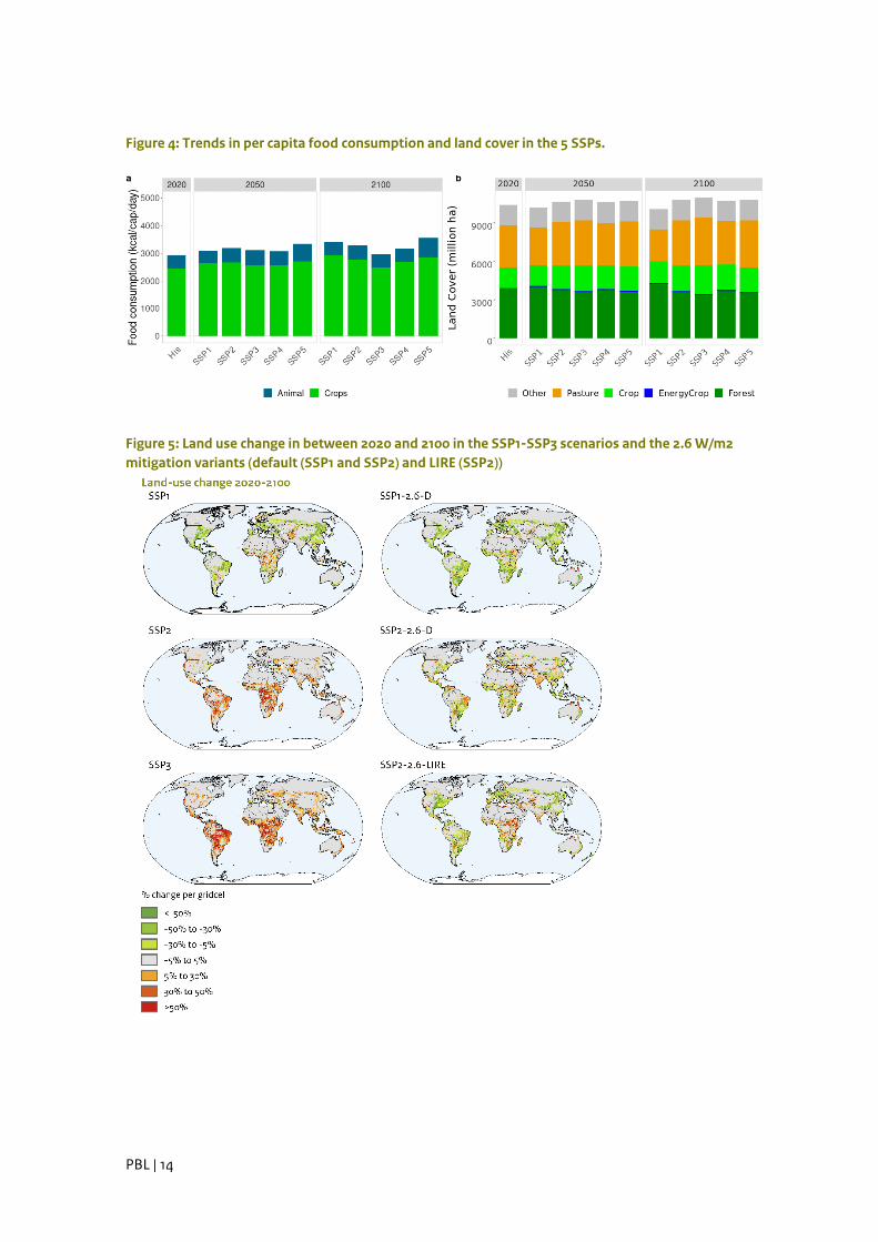
3.2 Food systems and land use The SSPs also lead to different scenarios in terms of food consumption, although some differences are partly counteracting at the aggregated level. In SSP1, low population growth and shifts to less meat intensive diets lead to lower demand for overall agriculture production. However, this is (at the level of per capita food consumption) partly offset by more rapid economic growth and the reduction of hunger. In SSP3, lower economic growth leads to somewhat lower food demand but a slightly higher meat share. However, in combination with population growth, this leads to a much higher overall food demand. For the other scenarios, similar trends can be identified (see Figure 4). Additional to the trends in food consumption, agricultural efficiency and production systems, trade, bio-energy use and climate policy drive the overall land-use dynamics. SSP1 shows substantial reductions in agricultural land use, related to relatively lower shares of animal product consumption, high agricultural efficiency, and string land protection. On the opposite end, the larger increase in food demand in SSP3 combined with low yield improvement leads to large increases in agricultural land and loss of natural land area. At a lower pace, the increase in the agricultural area also continues in SSP2 and SSP4, though regionally differentiated (SSP4 shows lower demand increase due to lower economic growth and low technology development). Agricultural expansion in SSP5 is mostly due to strong increases in per capita consumption. The trends in land use can also be seen at the grid level. While in the SSP1, there is mostly reforestation (green cells) in SSP3, there is mostly a deforestation trend (red cells). The SSP2 scenario shows a more intermediate position with modest reforestation in OECD countries and further deforestation in tropical areas.

PBL | 14

Figure 4: Trends in per capita food consumption and land cover in the 5 SSPs.

Figure 5: Land use change in between 2020 and 2100 in the SSP1-SSP3 scenarios and the 2.6 W/m2 mitigation variants (default (SSP1 and SSP2) and LIRE (SSP2))

PBL | 15

3.3 Greenhouse gas emissions Trends in the energy system and land use translate into emissions of greenhouse gases (Figure 6). The SSP1 scenario is indicative of the low-end range of scenarios without climate policy in the literature, given a very low increase in energy-related emissions and the decline of anthropogenic

land-use-related GHG emissions. The latter is, in fact, a combination of negative CO2 emissions from deforestation and the remaining CH4 and N2O emissions from agriculture. This trend continues in the 2050–2100 period, resulting in an overall decrease of emissions in 2100 of over 35% compared to today. The SSP2 and SSP3 scenarios follow an opposite trend in which emissions increase throughout the 21st century, more common for reference scenarios. Both SSP2 and SSP3 end up as median emission scenarios compared to the overall literature. Energy-related CO2 emissions mostly drive the increase in both scenarios. The SP5 scenario is clearly a high-end emission scenario.

Figure 6: Trends in greenhouse gas emissions expressed in CO2-eq, by source and type of gas (the bars represent SSP1 to SSP5, respectively)

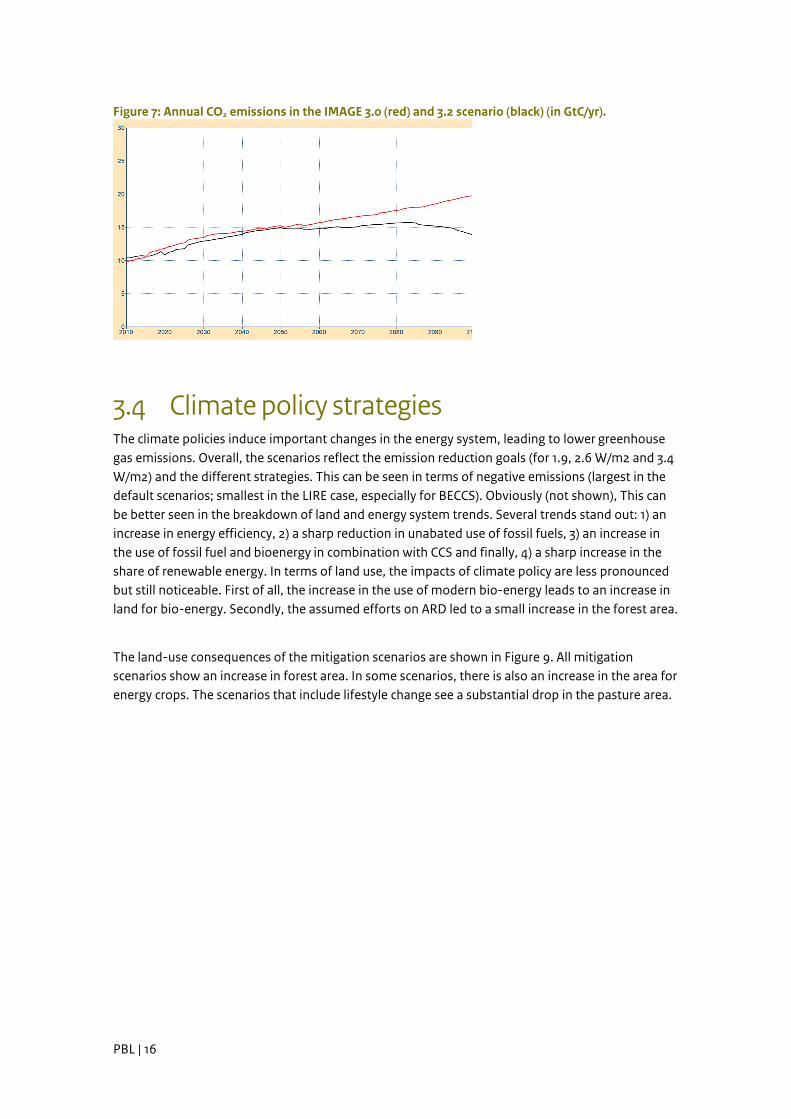
Figure 7 finally compares the annual CO2 emissions in the IMAGE 3.0 and 3.2 scenarios showing the short-lived emission reduction in 2020 (due to the COVID-19 pandemic) followed by somewhat lower emissions in subsequent years. After 2050 the scenarios start to more clearly diverge due to lower technology costs for renewables and more rapid penetration of electric vehicles (the trend starts much earlier but becomes at the global level only clearly visible at that time).

PBL | 16

Figure 7: Annual CO2 emissions in the IMAGE 3.0 (red) and 3.2 scenario (black) (in GtC/yr).

3.4 Climate policy strategies The climate policies induce important changes in the energy system, leading to lower greenhouse gas emissions. Overall, the scenarios reflect the emission reduction goals (for 1.9, 2.6 W/m2 and 3.4 W/m2) and the different strategies. This can be seen in terms of negative emissions (largest in the default scenarios; smallest in the LIRE case, especially for BECCS). Obviously (not shown), This can be better seen in the breakdown of land and energy system trends. Several trends stand out: 1) an increase in energy efficiency, 2) a sharp reduction in unabated use of fossil fuels, 3) an increase in the use of fossil fuel and bioenergy in combination with CCS and finally, 4) a sharp increase in the share of renewable energy. In terms of land use, the impacts of climate policy are less pronounced but still noticeable. First of all, the increase in the use of modern bio-energy leads to an increase in land for bio-energy. Secondly, the assumed efforts on ARD led to a small increase in the forest area.

The land-use consequences of the mitigation scenarios are shown in Figure 9. All mitigation scenarios show an increase in forest area. In some scenarios, there is also an increase in the area for energy crops. The scenarios that include lifestyle change see a substantial drop in the pasture area.

PBL | 17

Figure 8: Emission trends and emission sources in the various mitigation variants

Figure 9: Land use in 2050 and 2100 in the various mitigation variants

PBL | 18

4 Conclusions In this paper, we describe a new set of possible pathways of future energy use, land use, greenhouse gas emissions and climate change as implemented in IMAGE 3.2. The scenarios form an update of an earlier set of scenarios in IMAGE 3.0. The most important changes are the model updates (providing more detailed results), the impact of COVID-19 and the updates in recent data trends. As a result, in general, greenhouse gas emissions are somewhat lower than the previous set. The scenario set also includes a set of mitigation scenarios. Instead of providing only default mitigation scenarios, additional scenarios with lifestyle and renewable energy variants are included. Data can be obtained from the IMAGE website (https://www.pbl.nl/en/image/about-image) or requested from the IMAGE team.

PBL | 19

References 1. van Vuuren, D.P., et al., The representative concentration pathways: an overview. Climatic Change, 2011. 109(1-2): p. 5-31. 2. Riahi, K., et al., The Shared Socioeconomic Pathways and their energy, land use, and greenhouse gas emissions implications: An overview. Global Environmental Change, 2017. 42: p. 153-168. 3. O'Neill, B.C., et al., The roads ahead: Narratives for shared socioeconomic pathways describing world futures in the 21st century. Global Environmental Change, 2017. 42: p. 169-180. 4. van Vuuren, D.P., et al., The Shared Socio-economic Pathways: Trajectories for human development and global environmental change. Global Environmental Change, 2017. 42: p. 148-152. 5. IPCC, Climate Change 2021 - The Physical Science Basis. Summary for Policymakers. 2021, Working Group I contribution to the Sixth Assessment Report of the Intergovernmental Panel on Climate Change. 6. IPCC, Global Warming of 1.5 °C. 2018, Intergovernmental panel on climate change: Geneva, Switserland. 7. Unccd, Global land outlook. 2017, United Nations Convetion to Combat Desertification. 8. O’Neill, B.C., et al., Achievements and needs for the climate change scenario framework. Nature Climate Change, 2020. 10(12): p. 1074-1084. 9. Van Vuuren, D.P., et al., Energy, land-use and greenhouse gas emissions trajectories under a green growth paradigm. Global Environmental Change, 2017. 42: p. 237-250. 10. Woltjer, G.B., et al., The Magnet Model − Module Description. 2014. 11. Schaphoff, S., et al., LPJmL4 – a dynamic global vegetation model with managed land – Part 1: Model description. Geosci. Model Dev., 2018. 11(4): p. 1343-1375. 12. Müller, C., et al., Drivers and patterns of land biosphere carbon balance reversal. Environmental Research Letters, 2016. 11(4). 13. Cengic, M., et al., Global 10 arc-seconds land suitability maps for projecting future agricultural expansion. DANS EASY, 2020. 14. Meinshausen, M., S.C.B. Raper, and T.M.L. Wigley, Emulating coupled atmosphere-ocean and carbon cycle models with a simpler model, MAGICC6 - Part 1: Model description and calibration. Atmospheric Chemistry and Physics, 2011. 11(4): p. 1417-1456. 15. Stehfest, E., et al., eds. IMAGE 3.0. 2014, PBL Netherlands Environmental Assessment Agency. 16. Daioglou, V., et al., he role of efficiency improvement and technology choice in energy and emissions reduction of the residential sector. Energy, 2021. under review. 17. de Boer, H.S.H.S. and D.D.P. van Vuuren, Representation of variable renewable energy sources in TIMER, an aggregated energy system simulation model. Energy Economics, 2017. 64: p. 600-611. 18. Daioglou, V., et al., Greenhouse gas emission curves for advanced biofuel supply chains. Nature Climate Change, 2017. 7(12): p. 920-924. 19. Daioglou, V., et al., Bioenergy technologies in long-run climate change mitigation: results from the EMF-33 study. Climatic Change, 2020. 163(3): p. 1603-1620. 20. Gernaat, D.E.H.J., et al., Climate change impacts on renewable energy supply. Nature Climate Change, 2021. 11(2): p. 119-125. 21. van Zeist, W.-J., et al., Are scenario projections overly optimistic about future yield progress? Global Environmental Change, 2020. 64: p. 102120. 22. Doelman, J.C., et al., Afforestation for climate change mitigation: Potentials, risks and trade-offs. Global Change Biology, 2020. 26(3): p. 1576-1591.

PBL | 20

23. Frank, S., et al., Agricultural non-CO2 emission reduction potential in the context of the 1.5 °C target. Nature Climate Change, 2019. 9(1): p. 66-72. 24. de Vos, L., et al., Trade-offs between water needs for food, utilities, and the environment - a nexus quantification at different scales. Environmental Research Letters, 2021. 25. Harmsen, J.H.M., et al., Long-term marginal abatement cost curves of non-CO<inf>2</inf> greenhouse gases. Environmental Science and Policy, 2019. 99: p. 136-149. 26. Kc, S. and W. Lutz, The human core of the shared socioeconomic pathways: Population scenarios by age, sex and level of education for all countries to 2100. Global Environmental Change, 2017. 42: p. 181-192. 27. IMF, World Economic Outlook Update, June 2020: A Crisis Like No Other, An Uncertain Recovery https://www.imf.org/en/Publications/WEO/Issues/2020/06/24/WEOUpdateJune2020. 2020, International Monetary Fund. 28. Dellink, R., et al., Long-term economic growth projections in the Shared Socioeconomic Pathways. Global Environmental Change, 2017. 42: p. 200-214. 29. Doelman, J.C., et al., Exploring SSP land-use dynamics using the IMAGE model: Regional and gridded scenarios of land-use change and land-based climate change mitigation. Global Environmental Change, 2018. 48: p. 119-135. 30. Kriegler, E., et al., A new scenario framework for climate change research: The concept of shared climate policy assumptions. Climatic Change, 2014. 122(3): p. 401-414. 31. Daioglou, V., et al., Energy demand and emissions of the non-energy sector. Energy and Environmental Science, 2014. 7(2): p. 482-498. 32. Daioglou, V., et al., Projections of the availability and cost of residues from agriculture and forestry. GCB Bioenergy, 2016. 8(2): p. 456-470. 33. Rao, S., et al., Future air pollution in the Shared Socio-economic Pathways. Global Environmental Change, 2017. 42: p. 346-358.

PBL | 21

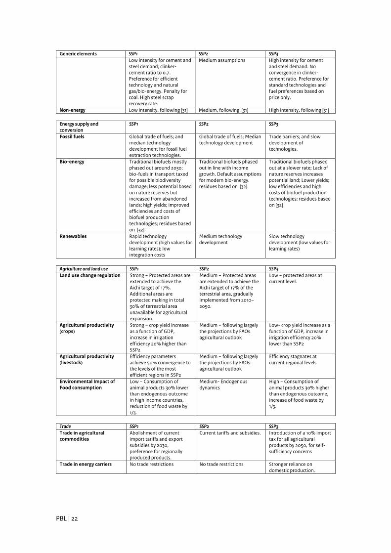
Appendix A: Assumptions for baselines Table 1. Generic description of the storyline elements and their translation to model assumptions for SSP1, SSP2, and SSP3 in IMAGE (indications high and low are made in comparison to a median development path). [9]

Generic elements SSP1 SSP2 SSP3

Economic growth High, based on [28] Medium, based on [28] Low, based on [28]

Population growth Low, based on [26] Medium, based on [26] High in developing countries;

low in developed countries,

based on [26]

Governance and institutions Effective both nationally and

internationally

Uneven International institutions

weak; security policies

Technology Rapid, translated into for

instance in assumptions for

efficiency, renewable

technologies and yields

Medium Slow

Consumption/production

preferences

Promotion of sustainable

development (lower

consumption − see further)

Medium Relative resource intensive

consumption

Energy demand SSP1 SSP2 SSP3 Transport Lower share of income spent

on transport leading to less kms travelled. More travel time (0,5 min/day increase each yr) resulting in less shift to faster modes. Preference for public transport, car sharing, and faster increase in efficiency (10% in 2100).

Medium assumptions Slower reduction of costs and efficiency increase of new technologies. Higher share of income spend on transport and later saturation of transport demand. No increase in travel-time implying a more rapid shift to high speed modes.

Buildings Behavioural changes lead to overall lower demand for energy services (heating, cooling, appliances). Adoption of more efficient technologies. Faster rural electrification. Rapid phase out of traditional fuels.

Medium assumptions Slower improvement rates of efficient technologies.Low improvements towards access to modern energy carriers

Industry Low intensity for cement and steel demand; clinker-cement ratio to 0.7. Preference for efficient technology and natural gas/bio-energy. Penalty for coal. High steel scrap recovery rate.

Medium assumptions High intensity for cement and steel demand. No convergence in clinker-cement ratio. Preference for standard technologies and fuel preferences based on price only.

PBL | 22

Generic elements SSP1 SSP2 SSP3 Low intensity for cement and

steel demand; clinker-cement ratio to 0.7. Preference for efficient technology and natural gas/bio-energy. Penalty for coal. High steel scrap recovery rate.

Medium assumptions High intensity for cement and steel demand. No convergence in clinker-cement ratio. Preference for standard technologies and fuel preferences based on price only.

Non-energy Low intensity, following [31] Medium, following [31] High intensity, following [31]

Energy supply and conversion

SSP1 SSP2 SSP3

Fossil fuels Global trade of fuels; and median technology development for fossil fuel extraction technologies.

Global trade of fuels; Median technology development

Trade barriers; and slow development of technologies.

Bio-energy Traditional biofuels mostly phased out around 2030; bio-fuels in transport taxed for possible biodiversity damage; less potential based on nature reserves but increased from abandoned lands; high yields; improved efficiencies and costs of biofuel production technologies; residues based on [32]

Traditional biofuels phased out in line with income growth. Default assumptions for modern bio-energy. residues based on [32].

Traditional biofuels phased out at a slower rate; Lack of nature reserves increases potential land; Lower yields; low efficiencies and high costs of biofuel production technologies; residues based on [32]

Renewables Rapid technology development (high values for learning rates); low integration costs

Medium technology development

Slow technology development (low values for learning rates)

Agriculture and land use SSP1 SSP2 SSP3 Land use change regulation Strong − Protected areas are

extended to achieve the Aichi target of 17%. Additional areas are protected making in total 30% of terrestrial area unavailable for agricultural expansion.

Medium − Protected areas are extended to achieve the Aichi target of 17% of the terrestrial area, gradually implemented from 2010–2050.

Low − protected areas at current level.

Agricultural productivity (crops)

Strong − crop yield increase as a function of GDP, increase in irrigation efficiency 20% higher than SSP2

Medium − following largely the projections by FAOs agricultural outlook

Low- crop yield increase as a function of GDP, increase in irrigation efficiency 20% lower than SSP2

Agricultural productivity (livestock)

Efficiency parameters achieve 50% convergence to the levels of the most efficient regions in SSP2

Medium − following largely the projections by FAOs agricultural outlook

Efficiency stagnates at current regional levels

Environmental Impact of Food consumption

Low − Consumption of animal products 30% lower than endogenous outcome in high income countries, reduction of food waste by 1/3.

Medium- Endogenous dynamics

High − Consumption of animal products 30% higher than endogenous outcome, increase of food waste by 1/3.

Trade SSP1 SSP2 SSP3 Trade in agricultural commodities

Abolishment of current import tariffs and export subsidies by 2030, preference for regionally produced products.

Current tariffs and subsidies. Introduction of a 10% import tax for all agricultural products by 2050, for self- sufficiency concerns

Trade in energy carriers No trade restrictions No trade restrictions Stronger reliance on domestic production.

PBL | 23

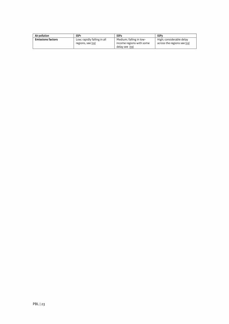
Air pollution SSP1 SSP2 SSP3 Emissions factors Low; rapidly falling in all

regions, see [33] Medium; falling in low-income regions with some delay see [33]

High; considerable delay across the regions see [33]