Embed Size (px)
Citation preview
Publ. Astron. Soc. Japan (2015) 67 (3), 50 (1–22)doi: 10.1093/pasj/psv022
50-1
The AKARI far-infrared all-sky survey maps
Yasuo DOI,1,∗ Satoshi TAKITA,2 Takafumi OOTSUBO,1 Ko ARIMATSU,2
Masahiro TANAKA,3 Yoshimi KITAMURA,2 Mitsunobu KAWADA,2
Shuji MATSUURA,2 Takao NAKAGAWA,2 Takahiro MORISHIMA,4
Makoto HATTORI,4 Shinya KOMUGI,2,† Glenn J. WHITE,5,6 Norio IKEDA,2
Daisuke KATO,2 Yuji CHINONE,4,‡ Mireya ETXALUZE,5,6
and Elysandra F. CYPRIANO7,5
1Department of Earth Science and Astronomy, The University of Tokyo, 3-8-1 Komaba, Meguro-ku,Tokyo 153-8902, Japan
2Institute of Space and Astronautical Science, Japan Aerospace Exploration Agency, 3-1-1 Yoshinodai,Chuo-ku, Sagamihara, Kanagawa 252-5210, Japan
3Center for Computational Sciences, University of Tsukuba, 1-1-1 Tennodai, Tsukuba, Ibaraki 305-8577,Japan
4Astronomical Institute, Tohoku University, Aramaki, Aoba-ku, Sendai, Miyagi 980-8578, Japan5Department of Physics & Astronomy, The Open University, Milton Keynes, MK7 6BJ, UK6Space Science and Technology Department, The Rutherford Appleton Laboratory, Didcot OX11 0QX, UK7Department of Astronomy, IAG, Universidade de Sao Paulo, 05508-090 Sao Paulo, SP, Brazil
*E-mail: [email protected]†Present address: Division of Liberal Arts, Kogakuin University, 2665-1 Nakano-machi, Hachioji, Tokyo 192-0015, Japan.‡Present address: High Energy Accelerator Research Organization (KEK), 1-1 Oho, Tsukuba, Ibaraki 305-0801, Japan.
Received 2014 December 19; Accepted 2015 March 20
Abstract
We present a far-infrared all-sky atlas from a sensitive all-sky survey using the JapaneseAKARI satellite. The survey covers > 99% of the sky in four photometric bands centred at65 µm, 90 µm, 140 µm, and 160 µm, with spatial resolutions ranging from 1′ to 1 .′′5. Thesedata provide crucial information on the investigation and characterisation of the proper-ties of dusty material in the interstellar medium (ISM), since a significant portion of itsenergy is emitted between ∼ 50 and 200 µm. The large-scale distribution of interstellarclouds, their thermal dust temperatures, and their column densities can be investigatedwith the improved spatial resolution compared to earlier all-sky survey observations. Inaddition to the point source distribution, the large-scale distribution of ISM cirrus emis-sion, and its filamentary structure, are well traced. We have made the first public releaseof the full-sky data to provide a legacy data set for use in the astronomical community.
Key words: atlases — Galaxy: general — infrared: galaxies — ISM: general — surveys
1 Introduction
Infrared continuum emission is ubiquitous across the sky,and is attributed to the thermal emission from interstellar
dust particles. These interstellar dust particles are heatedby an incident stellar radiation field of UV, optical,and near-infrared wavelengths—interstellar radiation field
C© The Authors 2015. Published by Oxford University Press on behalf of The Royal Astronomical Society. This is an Open Access articledistributed under the terms of the Creative Commons Attribution License (http://creativecommons.org/licenses/by/4.0/), which permitsunrestricted reuse, distribution, and reproduction in any medium, provided the original work is properly cited.
by guest on June 5, 2015http://pasj.oxfordjournals.org/
Dow
nloaded from
50-2 Publications of the Astronomical Society of Japan (2015), Vol. 67, No. 3
(ISRF)—which together have an energy peak at around1 µm (Mathis et al. 1983). The heated dust radiates itsthermal energy at longer wavelengths in the infrared to mil-limetre wavelength range. The spectral energy distribution(SED) of the dust continuum emission has been observedfrom various astronomical objects including the diffuseinterstellar medium (ISM), star-formation regions, andgalaxies. The observed SEDs show their peak at far-infrared(FIR) wavelength (30–300 µm), with approximately twothirds of the energy being radiated at λ ≥ 50 µm (Draine2003; also see Compiegne et al. 2011). It is thus importantto measure the total FIR continuum emission energy as itis a good tracer of total stellar radiation energy, which isdominated by the radiation from young OB-stars, and thusa good indicator of the star-formation activity (Kennicutt1998).
The first all-sky survey of infrared continuum between12 and 100 µm was pioneered by the IRAS satellite(Neugebauer et al. 1984). It carried out a photometricsurvey with two FIR photometric bands centred at 60 µmand 100 µm, achieving a spatial resolution of ∼ 4′. TheIRAS observation was designed to detect point sources,but not to undertake absolute photometry (Beichman et al.1988), leaving the surface brightness of diffuse emissionwith spatial scales larger than ∼ 5′ to be measured onlyrelatively. It has, however, been possible to create large-area sky maps (the IRAS Sky Survey Atlas: ISSA; Wheelocket al. 1994), by filtering out detector sensitivity drifts. Animprovement on the efficacy of the IRAS diffuse emissiondata was made by combining absolute photometry datawith lower spatial resolution from COBE/DIRBE observa-tions (Boggess et al. 1992; Hauser et al. 1998), and byusing an improved image destriping technique (ImprovedReprocessing of the IRAS Survey: IRIS; Miville-Deschenes& Lagache 2005). An all-sky survey at submillimetre (sub-mm) wavelengths from 350 µm–10 mm was made by thePlanck satellite with an angular resolution from 5′ to 33′
(Planck Collaboration 2014a).The observed FIR dust continuum SEDs are reason-
ably well fitted with modified blackbody spectra that havespectral indices β ∼ 1.5–2, with temperatures ∼ 15–20 K(Boulanger et al. 1996; Lagache et al. 1998; Draine 2003;Roy et al. 2010; Planck Collaboration 2011; Planck Col-laboration 2014b; Meisner & Finkbeiner 2015). Dust parti-cles with relatively larger sizes (big grains: BG; a ≥ 0.01 µmwith a typical size of a ∼ 0.1 µm) are considered to be themain source of this FIR emission (Desert et al. 1990; Mathis1990; Draine & Li 2007; Compiegne et al. 2011). The BGsare in thermal equilibrium with the ambient ISRF and thustheir temperatures (TBG) trace the local ISRF intensity (IISRF;Compiegne et al. 2010; Bernard et al. 2010). Measuring theSED of the BG emitters both above, and below, the peak
of the SED, is therefore important for determining TBG.For the diffuse ISM, we can assume a uniform TBG alongthe line of sight and thus can convert the observed TBG
to IISRF.The opacity of the BGs (τBG) of the diffuse clouds can
be evaluated from the observed FIR intensity and TBG.Assuming that dust and gas are well mixed in interstellarspace, τBG is a good tracer of the total gas column densityincluding all the interstellar components: atomic, molec-ular, and ionized gas (e.g., Boulanger & Perault 1988;Joncas et al. 1992; Boulanger et al. 1996; Bernard et al.1999; Lagache et al. 2000; Miville-Deschenes et al. 2007;Planck Collaboration 2011). It is also important to useestimates of τBG as a proxy to infer the foreground tothe cosmic microwave background (CMB) emission thatis observed in longer wavelengths (Schlegel et al. 1998;Miville-Deschenes & Lagache 2005; Compiegne et al.2011; Planck Collaboration 2014a, 2014b; Meisner &Finkbeiner 2015).
Since the IRAS observations cover only the wavelengthsat, or shorter than, 100 µm, it is important to note that emis-sion from stochastically heated smaller dust grains becomessignificant at shorter wavelengths. Compiegne et al. (2010)estimated the contribution of smaller dust emission to theirobservations with the PACS instrument (Poglitsch et al.2010) onboard the Herschel satellite (Pilbratt et al. 2010)based on their adopted dust model (Compiegne et al. 2011).They estimated the contribution to be up to ∼ 50% in the70 µm band, ∼ 17% in the 100 µm band, and up to ∼ 7% inthe 160 µm band, and concluded that photometric observa-tions at ≤ 70 µm should be modelled by taking into accountthe significant contribution of emission from stochasticallyheated grains. To make accurate TBG determination withoutsuffering effects from the excess emission from stochasti-cally heated smaller dust grains, the IRAS data thus needto be combined with longer wavelength COBE/DIRBE orPlanck data (Schlegel et al. 1998; Planck Collaboration2014b; Meisner & Finkbeiner 2015) or to be fitted witha modelled SED of the dust continuum (Planck Collabo-ration 2014c). However, COBE/DIRBE data have limitedspatial resolution of a 0 .◦7 × 0 .◦7 field-of-view (Hauser et al.1998). Planck data have a spatial resolution that is compa-rable with that of IRAS, but the data do not cover thepeak of the dust SED. Observations that cover the peakwavelength of the BG thermal emission with higher spatialresolutions are therefore required.
The ubiquitous distribution of diffuse infrared emission(cirrus emission) was first discovered by IRAS observations(Low et al. 1984). Satellite and balloon observations haverevealed that the cirrus emission has no characteristic spa-tial scales, and is well represented by Gaussian randomfields with a power-law spectrum ∝ k−3.0 (Gautier et al.
by guest on June 5, 2015http://pasj.oxfordjournals.org/
Dow
nloaded from
Publications of the Astronomical Society of Japan (2015), Vol. 67, No. 3 50-3
1992; Kiss et al. 2001, 2003; Miville-Deschenes et al. 2002,2007; Jeong et al. 2005; Roy et al. 2010), down to sub-arcminute scales (Miville-Deschenes et al. 2010; Martinet al. 2010). Recently, observations with Herschel witha high spatial resolution (12′′–18′′ at 70, 100, 160, and250 µm) resolved cirrus spatial structures in nearby star-forming regions, showing that they were dominated by fil-amentary structures. These filament structures have showntypical widths of ∼ 0.1 pc, which is common for all the fila-ments of those observed in the nearby Gould Belt clouds (cf.Arzoumanian et al. 2011; see also Arzoumanian et al. 2013and a comprehensive review by Andre 2015). Prestellarcores are observed to be concentrated on the filaments(Konyves et al. 2010; Andre et al. 2010), suggesting thatthe filamentary structure plays a prominent role in the starformation process (Andre et al. 2014). To reveal the mech-anism of the very first stages of the star formation process,the spatial scale of which changes from that of giant molec-ular clouds (≥ 100 pc) to the pre-stellar cores (≤ 0.1 pc), awider field survey with a high spatial resolution is requiredso that we can investigate the distribution of the cirrusemission across a broad range of spatial scales, to study itsnature in more detail, so as to remove its contribution as aforeground to the CMB.
For these reasons described above, we have performeda new all-sky survey with an infrared astronomical satel-lite AKARI (Murakami et al. 2007). The sky coverageof this survey was 99%, with 97% of the sky coveredwith multiple scans. The observed wavelength spans 50–180 µm continuously with four photometric bands, cen-tred at 65 µm, 90 µm, 140 µm, and 160 µm, which havespatial resolutions of 1′–1 .′5. The detection limit of thefour bands reaches 2.5–16 MJy sr−1 with relative accuracyof < 20%.
In this paper, we describe the details of the observationand the data analysis procedure. We also discuss the suit-ability of the data to measure the SED and estimate thespectral peak of the dust emission (so as to investigate thetotal FIR emission energy), and to determine the spatialdistribution of the interstellar matter and star-formationactivity at a high spatial resolution.
In section 2, we describe the observation made withour FIR instrument aboard AKARI. The details of thedata analysis are given in section 3, including subtractionof foreground zodiacal emission, the correction scheme oftransient response of FIR detectors, and image destriping.Characteristics of the produced images and their quality aredescribed in section 4. In section 5, we describe the capa-bility of the AKARI image to make the detailed evaluationof the spatial distribution and the SED of the interstellardust emission. The caveats that we have about remainingartefacts in the images, and our future plans to mitigate
the effects of these, are described in section 6. Informationon the data release is given in section 7. In section 8, wesummarize the results.
2 Observation
We performed an all-sky survey observation with theAKARI satellite, a dedicated satellite for infrared astro-nomical observations (Murakami et al. 2007). Its telescopemirror had a diameter of φ = 685 mm and was capable ofobserving across the 2–180 µm near-infrared (NIR) to FIRspectral regions, with two focal-plane instruments (FPIs):the InfraRed Camera (IRC: Onaka et al. 2007) and the Far-Infrared Surveyor (FIS: Kawada et al. 2007). Both of theFPIs, as well as the telescope, were cooled down to 6 K withliquid helium cryogen and mechanical double-stage Stirlingcoolers as a support (Nakagawa et al. 2007), reducing theinstrumental thermal emission. The satellite was launchedin 2006 February and the all-sky survey was performedduring the period 2006 April–2007 August, which was thecold operational phase of the satellite with liquid heliumcryogen.
The satellite was launched into a Sun-synchronous polarorbit with an altitude of 700 km, an inclination angle of98 .◦2, and an orbital period of 98 min, so that the satelliterevolved along the day–night boundary of the Earth. Duringthe survey observations, the pointing direction of the tele-scope was kept orthogonal to the Sun–Earth direction andwas kept away from the centre of the Earth. Consequently,the radiative heat input from the Sun to the satellite waskept constant and that from the Earth was minimized (seefigure 4 of Murakami et al. 2007).
With this orbital configuration, the AKARI telescopecontinuously scanned the sky along the great circle with aconstant scan speed of 3 .′6 s−1. Due to the yearly revolutionof the Earth, the scan direction is shifted ∼ 4′ per satelliterevolution in a longitudinal direction or in the cross-scandirection. Consequently it was possible to survey the wholesky during each six-month period of continuous observa-tion.
Dedicated pointed observations of specific astronom-ical objects were interspersed with survey observations(Murakami et al. 2007). The survey observation was haltedfor 30 minutes during a pointed observation to allow for10 minutes of integration time as well as the satellite’s atti-tude manoeuvre before and after the pointed observation.The regions that had been left unsurveyed due to pointedobservations were rescanned at a later time during the coldoperational phase.
The all-sky survey observations at FIR wavelengthswere performed using the FIS instrument, which wasdedicated for photometric scans and spectroscopic
by guest on June 5, 2015http://pasj.oxfordjournals.org/
Dow
nloaded from
50-4 Publications of the Astronomical Society of Japan (2015), Vol. 67, No. 3
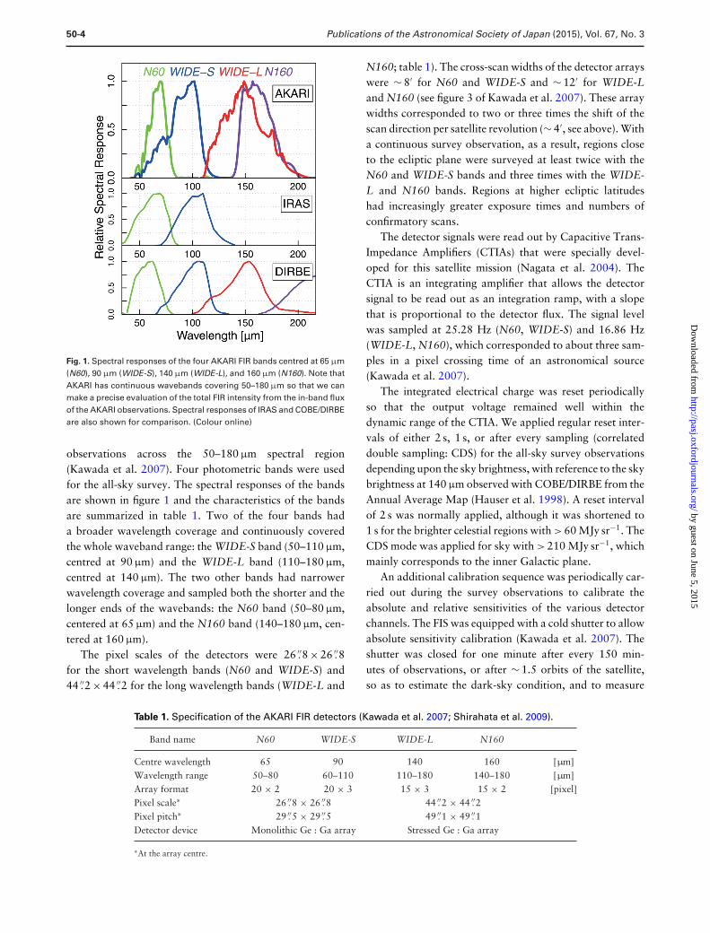
Fig. 1. Spectral responses of the four AKARI FIR bands centred at 65 µm(N60), 90 µm (WIDE-S), 140 µm (WIDE-L), and 160 µm (N160). Note thatAKARI has continuous wavebands covering 50–180 µm so that we canmake a precise evaluation of the total FIR intensity from the in-band fluxof the AKARI observations. Spectral responses of IRAS and COBE/DIRBEare also shown for comparison. (Colour online)
observations across the 50–180 µm spectral region(Kawada et al. 2007). Four photometric bands were usedfor the all-sky survey. The spectral responses of the bandsare shown in figure 1 and the characteristics of the bandsare summarized in table 1. Two of the four bands hada broader wavelength coverage and continuously coveredthe whole waveband range: the WIDE-S band (50–110 µm,centred at 90 µm) and the WIDE-L band (110–180 µm,centred at 140 µm). The two other bands had narrowerwavelength coverage and sampled both the shorter and thelonger ends of the wavebands: the N60 band (50–80 µm,centered at 65 µm) and the N160 band (140–180 µm, cen-tered at 160 µm).
The pixel scales of the detectors were 26 .′′8 × 26 .′′8for the short wavelength bands (N60 and WIDE-S) and44 .′′2 × 44 .′′2 for the long wavelength bands (WIDE-L and
N160; table 1). The cross-scan widths of the detector arrayswere ∼ 8′ for N60 and WIDE-S and ∼ 12′ for WIDE-Land N160 (see figure 3 of Kawada et al. 2007). These arraywidths corresponded to two or three times the shift of thescan direction per satellite revolution (∼ 4′, see above). Witha continuous survey observation, as a result, regions closeto the ecliptic plane were surveyed at least twice with theN60 and WIDE-S bands and three times with the WIDE-L and N160 bands. Regions at higher ecliptic latitudeshad increasingly greater exposure times and numbers ofconfirmatory scans.
The detector signals were read out by Capacitive Trans-Impedance Amplifiers (CTIAs) that were specially devel-oped for this satellite mission (Nagata et al. 2004). TheCTIA is an integrating amplifier that allows the detectorsignal to be read out as an integration ramp, with a slopethat is proportional to the detector flux. The signal levelwas sampled at 25.28 Hz (N60, WIDE-S) and 16.86 Hz(WIDE-L, N160), which corresponded to about three sam-ples in a pixel crossing time of an astronomical source(Kawada et al. 2007).
The integrated electrical charge was reset periodicallyso that the output voltage remained well within thedynamic range of the CTIA. We applied regular reset inter-vals of either 2 s, 1 s, or after every sampling (correlateddouble sampling: CDS) for the all-sky survey observationsdepending upon the sky brightness, with reference to the skybrightness at 140 µm observed with COBE/DIRBE from theAnnual Average Map (Hauser et al. 1998). A reset intervalof 2 s was normally applied, although it was shortened to1 s for the brighter celestial regions with > 60 MJy sr−1. TheCDS mode was applied for sky with > 210 MJy sr−1, whichmainly corresponds to the inner Galactic plane.
An additional calibration sequence was periodically car-ried out during the survey observations to calibrate theabsolute and relative sensitivities of the various detectorchannels. The FIS was equipped with a cold shutter to allowabsolute sensitivity calibration (Kawada et al. 2007). Theshutter was closed for one minute after every 150 min-utes of observations, or after ∼ 1.5 orbits of the satellite,so as to estimate the dark-sky condition, and to measure
Table 1. Specification of the AKARI FIR detectors (Kawada et al. 2007; Shirahata et al. 2009).
Band name N60 WIDE-S WIDE-L N160
Centre wavelength 65 90 140 160 [µm]Wavelength range 50–80 60–110 110–180 140–180 [µm]Array format 20 × 2 20 × 3 15 × 3 15 × 2 [pixel]Pixel scale∗ 26 .′′8 × 26 .′′8 44 .′′2 × 44 .′′2Pixel pitch∗ 29 .′′5 × 29 .′′5 49 .′′1 × 49 .′′1Detector device Monolithic Ge : Ga array Stressed Ge : Ga array
∗At the array centre.
by guest on June 5, 2015http://pasj.oxfordjournals.org/
Dow
nloaded from
Publications of the Astronomical Society of Japan (2015), Vol. 67, No. 3 50-5
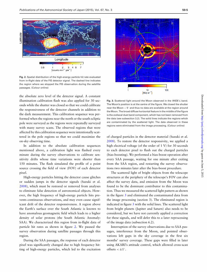
Fig. 2. Spatial distribution of the high-energy particle hit rate evaluatedfrom in-flight data of the FIS detector signal. The dashed line indicatesthe region where we stopped the FIS observation during the satellitepassages. (Colour online)
the absolute zero level of the detector signal. A constantillumination calibration flash was also applied for 30 sec-onds while the shutter was closed so that we could calibratethe responsiveness of the detector channels in addition tothe dark measurement. This calibration sequence was per-formed when the regions near the north or the south eclipticpole were surveyed as the regions were repeatedly surveyedwith many survey scans. The observed regions that wereaffected by this calibration sequence were intentionally scat-tered in the pole regions so that we could maximize theon-sky observing time.
In addition to the absolute calibration sequencesmentioned above, a calibration light was flashed everyminute during the survey observations to calibrate sen-sitivity drifts whose time variations were shorter than150 minutes. The flash simulated the profile of a pointsource crossing the field of view (FOV) of each detectorpixel.
High-energy particles hitting the detector cause glitchesor sudden jumps in the detector signals (Suzuki et al.2008), which must be restored or removed from analysesto eliminate false detection of astronomical objects. How-ever, the high frequency of high-energy particle hits pre-vents continuous observations, and may even cause signif-icant drift of the detector responsiveness. A region abovethe Earth’s surface over the South Atlantic is known tohave anomalous geomagnetic field which leads to a higherdensity of solar protons (the South Atlantic Anomaly:SAA). We characterized this region from in-flight data ofparticle hit rates as shown in figure 2. We paused thesurvey observation during satellite passages through thisregion.
During the SAA passages, the response of each detectorpixel was significantly changed due to high frequency hit-ting of high-energy particles, which led to the excitation
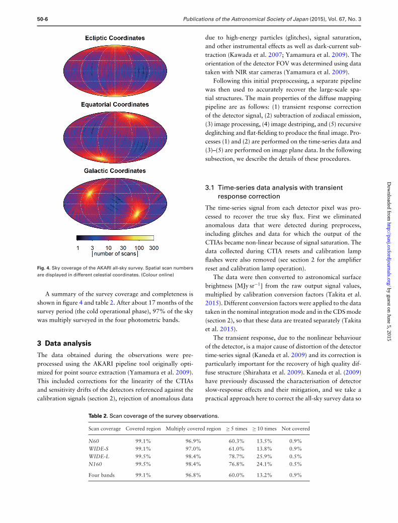
Fig. 3. Scattered light around the Moon observed in the WIDE-L band.The Moon’s position is at the centre of the figure. We closed the shutternear the Moon < 5◦ and thus no data are available at the region aroundthe Moon. The broad diffuse horizontal feature in the middle of the figureis the zodiacal dust band component, which has not been removed fromthe data (see subsection 3.2). The solid lines indicate the regions whichare contaminated by the scattered light. The data observed in theseregions were eliminated from the image processing. (Colour online)
of charged particles in the detector material (Suzuki et al.2008). To restore the detector responsivity, we applied ahigh electrical voltage (of the order of 1 V) for 30 secondsto each detector pixel to flush out the charged particles(bias-boosting). We performed a bias-boost operation afterevery SAA passage, waiting for one minute after exitingfrom the SAA region, and restarting the survey observa-tions two minutes later after the bias-boost procedure.
The scattered light of bright objects from the telescopestructures at the periphery of the telescope’s FOV can alsoaffect the survey data, and emission from the Moon wasfound to be the dominant contributor to this contamina-tion. Thus we measured the scattered light pattern as shownin the figure 3 and eliminated the contaminated data fromthe image processing (section 3). The eliminated region isindicated in figure 3 with the solid lines. The scattered lightfrom bright planets (Jupiter and Saturn) also needs to beconsidered, but we have not currently applied a correctionfor these signals, and will defer this to a later reprocessingof the image data (subsection 6.2).
Interruption of the survey observations due to SAA pas-sages, interference from the Moon, and pointed obser-vations left gaps in the sky coverage in the first sixmonths’ survey coverage. These gaps were filled in laterusing AKARI’s attitude control, which allowed cross-scanoffsets <±1◦.
by guest on June 5, 2015http://pasj.oxfordjournals.org/
Dow
nloaded from
50-6 Publications of the Astronomical Society of Japan (2015), Vol. 67, No. 3
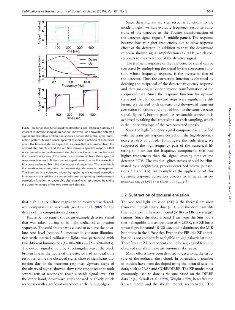
Fig. 4. Sky coverage of the AKARI all-sky survey. Spatial scan numbersare displayed in different celestial coordinates. (Colour online)
A summary of the survey coverage and completeness isshown in figure 4 and table 2. After about 17 months of thesurvey period (the cold operational phase), 97% of the skywas multiply surveyed in the four photometric bands.
3 Data analysis
The data obtained during the observations were pre-processed using the AKARI pipeline tool originally opti-mized for point source extraction (Yamamura et al. 2009).This included corrections for the linearity of the CTIAsand sensitivity drifts of the detectors referenced against thecalibration signals (section 2), rejection of anomalous data
due to high-energy particles (glitches), signal saturation,and other instrumental effects as well as dark-current sub-traction (Kawada et al. 2007; Yamamura et al. 2009). Theorientation of the detector FOV was determined using datataken with NIR star cameras (Yamamura et al. 2009).
Following this initial preprocessing, a separate pipelinewas then used to accurately recover the large-scale spa-tial structures. The main properties of the diffuse mappingpipeline are as follows: (1) transient response correctionof the detector signal, (2) subtraction of zodiacal emission,(3) image processing, (4) image destriping, and (5) recursivedeglitching and flat-fielding to produce the final image. Pro-cesses (1) and (2) are performed on the time-series data and(3)–(5) are performed on image plane data. In the followingsubsection, we describe the details of these procedures.
3.1 Time-series data analysis with transientresponse correction
The time-series signal from each detector pixel was pro-cessed to recover the true sky flux. First we eliminatedanomalous data that were detected during preprocess,including glitches and data for which the output of theCTIAs became non-linear because of signal saturation. Thedata collected during CTIA resets and calibration lampflashes were also removed (see section 2 for the amplifierreset and calibration lamp operation).
The data were then converted to astronomical surfacebrightness [MJy sr−1] from the raw output signal values,multiplied by calibration conversion factors (Takita et al.2015). Different conversion factors were applied to the datataken in the nominal integration mode and in the CDS mode(section 2), so that these data are treated separately (Takitaet al. 2015).
The transient response, due to the nonlinear behaviourof the detector, is a major cause of distortion of the detectortime-series signal (Kaneda et al. 2009) and its correction isparticularly important for the recovery of high quality dif-fuse structure (Shirahata et al. 2009). Kaneda et al. (2009)have previously discussed the characterisation of detectorslow-response effects and their mitigation, and we take apractical approach here to correct the all-sky survey data so
Table 2. Scan coverage of the survey observations.
Scan coverage Covered region Multiply covered region ≥ 5 times ≥ 10 times Not covered
N60 99.1% 96.9% 60.3% 13.5% 0.9%WIDE-S 99.1% 97.0% 61.0% 13.8% 0.9%WIDE-L 99.5% 98.4% 78.7% 25.9% 0.5%N160 99.5% 98.4% 76.8% 24.1% 0.5%
Four bands 99.1% 96.8% 60.0% 13.2% 0.9%
by guest on June 5, 2015http://pasj.oxfordjournals.org/
Dow
nloaded from
Publications of the Astronomical Society of Japan (2015), Vol. 67, No. 3 50-7
Fig. 5. Top panel: step function of the detector signal taken in-flight by aninternal calibration lamp illumination. The cyan line shows the detectedsignal and the black broken line shows a schematic of the lamp illumi-nation pattern. Middle panel: spectral response functions of a detectorpixel. The blue line shows a spectral response that is estimated from theupward step function and the red line shows a spectral response thatis estimated from the downward step function. Correction functions forthe transient response of the detector are evaluated from these spectralresponses (see text). Bottom panel: signal correction by the correctionfunctions evaluated from the above spectral responses. The cyan line isthe raw detector signal, which is the same signal shown in the top panel.The blue line is a corrected signal by applying the upward correctionfunction and the red line is a corrected signal by applying the downwardcorrection function. A reasonable signal profile is reproduced by takingthe upper envelope of the two corrected signals.
that high-quality diffuse maps can be recovered with real-istic computational overheads (see Doi et al. 2009 for thedetails of the computation scheme).
Figure 5, top panel, shows an example detector signalthat was taken during an in-flight dedicated calibrationsequence. The cold shutter was closed to achieve the abso-lute zero level (section 2), meanwhile constant illumina-tion with internal calibration lights was performed withtwo different luminosities (t = 80–200 s and t = 320–440 s).The output signal should be a rectangular wave (the blackbroken line in the figure) if the detector had an ideal timeresponse, while the observed signal showed significant dis-tortion due to the transient response. Upward steps ofthe observed signal showed slow time responses that tookseveral tens of seconds to reach a stable signal level. Onthe other hand, downward steps showed relatively quickresponses with significant overshoot at the falling edges.
Since these signals are step response functions to theincident light, we can evaluate frequency response func-tions of the detector as the Fourier transformation ofthe detector signal (figure 5, middle panel). The responsebecame low at higher frequencies due to slow-responseeffect of the detector. In addition to that, the downwardresponse showed signal amplification at < 1 Hz, which cor-responds to the overshoot of the detector signal.
The transient response of the raw detector signal can becorrected by multiplying the signal by the correction func-tion, whose frequency response is the inverse of that ofthe detector. Thus the correction function is obtained byderiving the reciprocal of the detector frequency responseand then making a Fourier inverse transformation of thereciprocal data. Since the response function for upwardsteps and that for downward steps were significantly dif-ferent, we derived both upward and downward transientcorrection functions and applied both to the same detectorsignal (figure 5, bottom panel). A reasonable correction isachieved by taking the larger signal at each sampling, whichis the upper envelope of the two corrected signals.
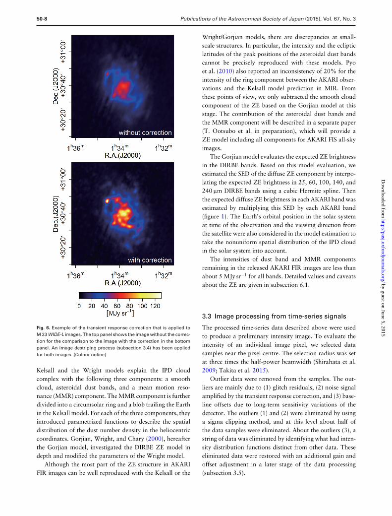
Since the high-frequency signal component is amplifiedwith the transient response correction, the high-frequencynoise is also amplified. To mitigate this side effect, wesuppressed the high-frequency part of the numerical fil-tering to filter out the frequency components that hadhigher frequencies than the signal crossing time of thedetector FOV. The residual glitch noises should be elim-inated by a deglitching process described below (subsec-tions 3.3 and 3.5). An example of the application of thistransient response correction process to an actual astro-nomical image (M 33) is shown in figure 6.
3.2 Subtraction of zodiacal emission
The zodiacal light emission (ZE) is the thermal emissionfrom the interplanetary dust (IPD) and the dominant dif-fuse radiation in the mid-infrared (MIR) to FIR wavelengthregions. Since the dust around 1 au from the Sun has athermal equilibrium temperature of ∼ 280 K, the ZE has aspectral peak around 10–20 µm, and it dominates the MIRbrightness in the diffuse sky. Even in the FIR, the ZE contri-bution is not completely negligible at high galactic latitude.Therefore the ZE component should be segregated from theobserved signal to make astronomical sky maps.
Many efforts have been devoted to describing the struc-ture of the zodiacal dust cloud. In particular, a numberof models have been developed using the infrared satellitedata, such as IRAS and COBE/DIRBE. The ZE model mostcommonly used to date is the one based on the DIRBEdata (e.g., Kelsall et al. 1998; Wright 1998; hereafter theKelsall model and the Wright model, respectively). The
by guest on June 5, 2015http://pasj.oxfordjournals.org/
Dow
nloaded from
50-8 Publications of the Astronomical Society of Japan (2015), Vol. 67, No. 3
Fig. 6. Example of the transient response correction that is applied toM 33 WIDE-L images. The top panel shows the image without the correc-tion for the comparison to the image with the correction in the bottompanel. An image destriping process (subsection 3.4) has been appliedfor both images. (Colour online)
Kelsall and the Wright models explain the IPD cloudcomplex with the following three components: a smoothcloud, asteroidal dust bands, and a mean motion reso-nance (MMR) component. The MMR component is furtherdivided into a circumsolar ring and a blob trailing the Earthin the Kelsall model. For each of the three components, theyintroduced parametrized functions to describe the spatialdistribution of the dust number density in the heliocentriccoordinates. Gorjian, Wright, and Chary (2000), hereafterthe Gorjian model, investigated the DIRBE ZE model indepth and modified the parameters of the Wright model.
Although the most part of the ZE structure in AKARIFIR images can be well reproduced with the Kelsall or the
Wright/Gorjian models, there are discrepancies at small-scale structures. In particular, the intensity and the eclipticlatitudes of the peak positions of the asteroidal dust bandscannot be precisely reproduced with these models. Pyoet al. (2010) also reported an inconsistency of 20% for theintensity of the ring component between the AKARI obser-vations and the Kelsall model prediction in MIR. Fromthese points of view, we only subtracted the smooth cloudcomponent of the ZE based on the Gorjian model at thisstage. The contribution of the asteroidal dust bands andthe MMR component will be described in a separate paper(T. Ootsubo et al. in preparation), which will provide aZE model including all components for AKARI FIS all-skyimages.
The Gorjian model evaluates the expected ZE brightnessin the DIRBE bands. Based on this model evaluation, weestimated the SED of the diffuse ZE component by interpo-lating the expected ZE brightness in 25, 60, 100, 140, and240 µm DIRBE bands using a cubic Hermite spline. Thenthe expected diffuse ZE brightness in each AKARI band wasestimated by multiplying this SED by each AKARI band(figure 1). The Earth’s orbital position in the solar systemat time of the observation and the viewing direction fromthe satellite were also considered in the model estimation totake the nonuniform spatial distribution of the IPD cloudin the solar system into account.
The intensities of dust band and MMR componentsremaining in the released AKARI FIR images are less thanabout 5 MJy sr−1 for all bands. Detailed values and caveatsabout the ZE are given in subsection 6.1.
3.3 Image processing from time-series signals
The processed time-series data described above were usedto produce a preliminary intensity image. To evaluate theintensity of an individual image pixel, we selected datasamples near the pixel centre. The selection radius was setat three times the half-power beamwidth (Shirahata et al.2009; Takita et al. 2015).
Outlier data were removed from the samples. The out-liers are mainly due to (1) glitch residuals, (2) noise signalamplified by the transient response correction, and (3) base-line offsets due to long-term sensitivity variations of thedetector. The outliers (1) and (2) were eliminated by usinga sigma clipping method, and at this level about half ofthe data samples were eliminated. About the outliers (3), astring of data was eliminated by identifying what had inten-sity distribution functions distinct from other data. Theseeliminated data were restored with an additional gain andoffset adjustment in a later stage of the data processing(subsection 3.5).
by guest on June 5, 2015http://pasj.oxfordjournals.org/
Dow
nloaded from
Publications of the Astronomical Society of Japan (2015), Vol. 67, No. 3 50-9
The residual data were weighted by distance from thepixel centre by assuming a Gaussian beam profile, whosefull width at half maximum was 30′′ for N60 and WIDE-S,and 50′′ for WIDE-L and N160, so that the beam widthwas comparable to the spatial resolution of the photometricbands and did not therefore degrade the spatial resolutionsof resultant images significantly. The weighted mean of theresidual data was then taken as the preliminary intensity ofthe image pixel. The weighted standard deviation, samplenumber, and spatial scan numbers were also recorded.
3.4 Image destriping
The resultant images show residual spatial stripes dueto imperfect flat-fielding caused by long-term sensitivityvariations of the detector. To eliminate this artificial pat-tern, we developed a destriping method based on Miville-Deschenes and Lagache (2005), who developed theirdestriping method to obtain the IRIS map. The details ofour procedure will be described in M. Tanaka et al. (inpreparation). We describe a brief summary in this paper.
The destriping method by Miville-Deschenes andLagache (2005) can be summarized as follows.
(i) Image decomposition: an input image is decomposedinto three components (a large-scale emission map, asmall-scale emission map, and a point-source map).
(ii) Stripe cleaning: the small-scale emission map is Fourier-transformed to obtain a spatial frequency map. Spatialfrequency components that are affected by the stripesare confined in the spatial frequency map along theradial directions that correspond to the stripe direc-tions in the original intensity map. The affected spatialfrequency components are replaced with magnitudesthat have averaged values along the azimuthal direction(see figure 1 of Miville-Deschenes & Lagache 2005).
(iii) Image restoration: the stripe-cleaned map is inverselyFourier-transformed and combined with the otherdecomposed images (a large-scale emission map anda point-source map).
We find that the stripe cleaning process of the small-scale emission map described above causes strong spu-rious patterns in some of the resultant images containingbright molecular clouds (e.g., Orion clouds). This is becausesuch regions contain small-scale and large-amplitude fluc-tuations of emission, which leads to contamination of thederived spatial spectrum over the spatial frequency domain.In this case, the subsequent destriping process unexpectedlymodifies the contaminated components of the spatial spec-trum and causes artefact patterns. Therefore, we masked theregions that showed large intensity variance in a small-scalemap and eliminated those regions from the stripe cleaning
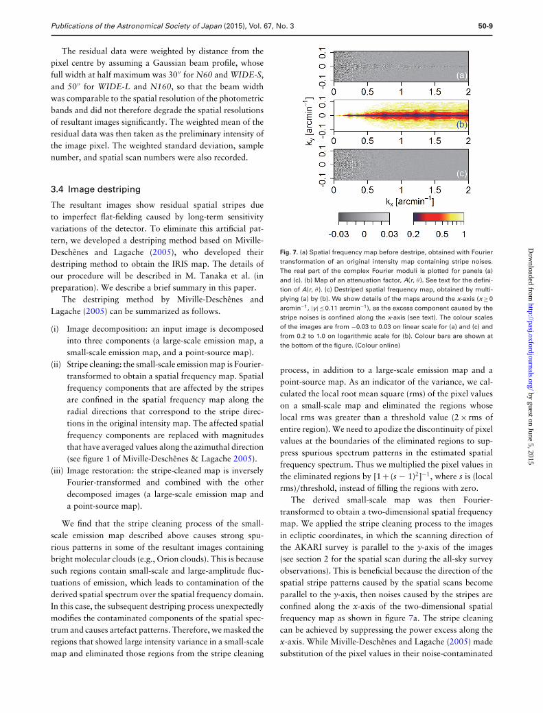
Fig. 7. (a) Spatial frequency map before destripe, obtained with Fouriertransformation of an original intensity map containing stripe noises.The real part of the complex Fourier moduli is plotted for panels (a)and (c). (b) Map of an attenuation factor, A(r, θ). See text for the defini-tion of A(r, θ). (c) Destriped spatial frequency map, obtained by multi-plying (a) by (b). We show details of the maps around the x-axis (x ≥ 0arcmin−1, |y| ≤ 0.11 arcmin−1), as the excess component caused by thestripe noises is confined along the x-axis (see text). The colour scalesof the images are from −0.03 to 0.03 on linear scale for (a) and (c) andfrom 0.2 to 1.0 on logarithmic scale for (b). Colour bars are shown atthe bottom of the figure. (Colour online)
process, in addition to a large-scale emission map and apoint-source map. As an indicator of the variance, we cal-culated the local root mean square (rms) of the pixel valueson a small-scale map and eliminated the regions whoselocal rms was greater than a threshold value (2 × rms ofentire region). We need to apodize the discontinuity of pixelvalues at the boundaries of the eliminated regions to sup-press spurious spectrum patterns in the estimated spatialfrequency spectrum. Thus we multiplied the pixel values inthe eliminated regions by [1 + (s − 1)2]−1, where s is (localrms)/threshold, instead of filling the regions with zero.
The derived small-scale map was then Fourier-transformed to obtain a two-dimensional spatial frequencymap. We applied the stripe cleaning process to the imagesin ecliptic coordinates, in which the scanning direction ofthe AKARI survey is parallel to the y-axis of the images(see section 2 for the spatial scan during the all-sky surveyobservations). This is beneficial because the direction of thespatial stripe patterns caused by the spatial scans becomeparallel to the y-axis, then noises caused by the stripes areconfined along the x-axis of the two-dimensional spatialfrequency map as shown in figure 7a. The stripe cleaningcan be achieved by suppressing the power excess along thex-axis. While Miville-Deschenes and Lagache (2005) madesubstitution of the pixel values in their noise-contaminated
by guest on June 5, 2015http://pasj.oxfordjournals.org/
Dow
nloaded from
50-10 Publications of the Astronomical Society of Japan (2015), Vol. 67, No. 3
regions with the azimuthal-averaged values, we multipliedthe spatial frequency map by an attenuation factor A(k),where k is a wavenumber vector, to suppress the powerexcess. This attenuation factor is similar to a filter in signalprocessing, which is used for converting an input spectrumF(k) to an output spectrum G(k) = A(k)F(k). Since a discon-tinuous filter function, such as a box-car function, causesripples on the result of Fourier transform, a smooth func-tion is better for suppressing artefact. Therefore, we calcu-lated the attenuation factor as follows. First we obtaineda power spectrum P(r, θ ), where (r, θ ) is a position on thetwo-dimensional spatial frequency map in the polar coordi-nate system. Next, we calculated the azimuthal average ofP(r, θ ) as Pa(r ), where a region around the x-axis wasexcluded from the averaging. Then, we calculated the localaverage of P(r, θ ) as Pl(r, θ ), in the range of r ± √
r/2 pixelsalong the radial direction of the spatial frequency map.Finally, the attenuation factor was calculated as
A(r, θ ) =
⎧⎪⎨⎪⎩
[Pa(r )/Pl(r, θ )]12 (if Pl(r, θ ) > Pa(r )
and (r, θ ) ∈ RA)1 (otherwise)
, (1)
where RA is a region around the x-axis defined by a partic-ular range in θ and y. Figure 7b shows an attenuation factormap obtained for a two-dimensional spatial frequency mapshown in figure 7a. Since Pl (r, θ ) is the local average ofP(r, θ ), A(r, θ ) has smooth distribution in the radial direc-tion. Figure 7b also shows that A(r, θ ) is close to unityif |y| > 0.05 arcmin−1, which means that our destripe pro-cess is not sensitive to the definition of RA. The resultantdestriped spatial frequency map is shown in figure 7c, whichis obtained by multiplying the spatial frequency map (a) bythe attenuation factor (b). The result shows that the spatialfrequency is attenuated down to the level of the azimuthalaverage.
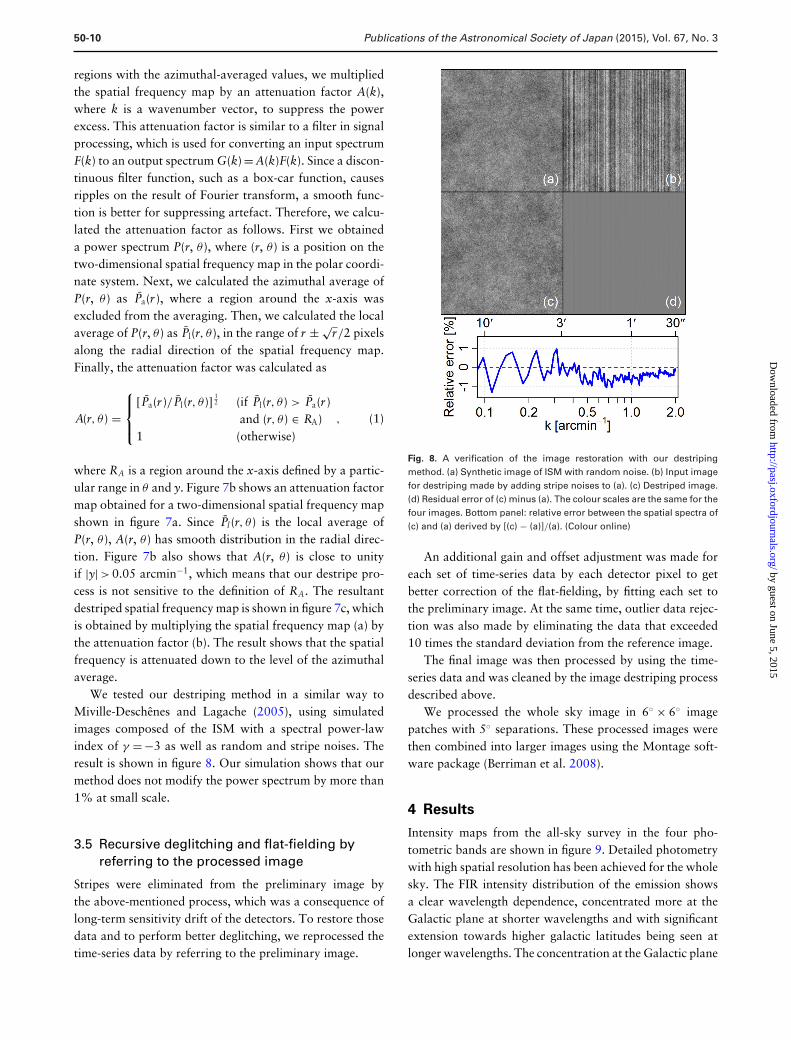
We tested our destriping method in a similar way toMiville-Deschenes and Lagache (2005), using simulatedimages composed of the ISM with a spectral power-lawindex of γ =−3 as well as random and stripe noises. Theresult is shown in figure 8. Our simulation shows that ourmethod does not modify the power spectrum by more than1% at small scale.
3.5 Recursive deglitching and flat-fielding byreferring to the processed image
Stripes were eliminated from the preliminary image bythe above-mentioned process, which was a consequence oflong-term sensitivity drift of the detectors. To restore thosedata and to perform better deglitching, we reprocessed thetime-series data by referring to the preliminary image.
Fig. 8. A verification of the image restoration with our destripingmethod. (a) Synthetic image of ISM with random noise. (b) Input imagefor destriping made by adding stripe noises to (a). (c) Destriped image.(d) Residual error of (c) minus (a). The colour scales are the same for thefour images. Bottom panel: relative error between the spatial spectra of(c) and (a) derived by [(c) − (a)]/(a). (Colour online)
An additional gain and offset adjustment was made foreach set of time-series data by each detector pixel to getbetter correction of the flat-fielding, by fitting each set tothe preliminary image. At the same time, outlier data rejec-tion was also made by eliminating the data that exceeded10 times the standard deviation from the reference image.
The final image was then processed by using the time-series data and was cleaned by the image destriping processdescribed above.
We processed the whole sky image in 6◦ × 6◦ imagepatches with 5◦ separations. These processed images werethen combined into larger images using the Montage soft-ware package (Berriman et al. 2008).
4 Results
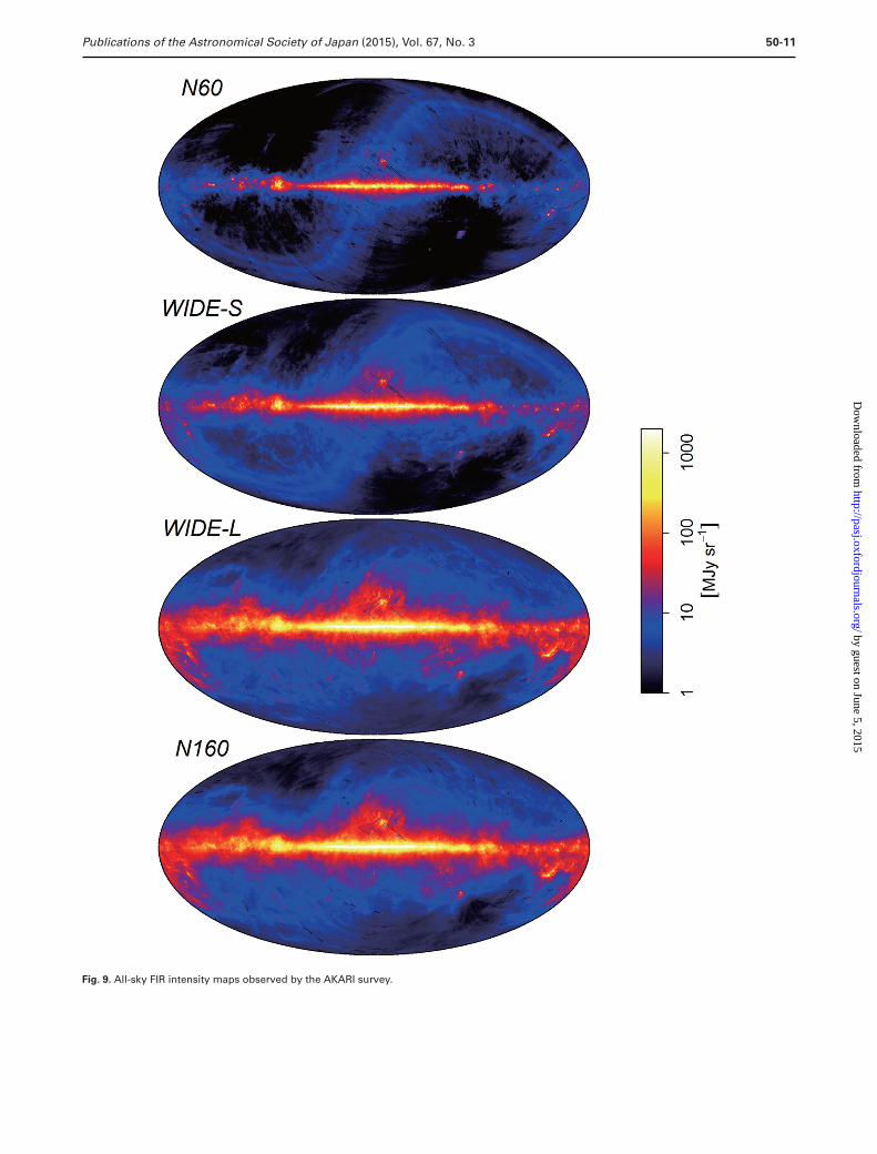
Intensity maps from the all-sky survey in the four pho-tometric bands are shown in figure 9. Detailed photometrywith high spatial resolution has been achieved for the wholesky. The FIR intensity distribution of the emission showsa clear wavelength dependence, concentrated more at theGalactic plane at shorter wavelengths and with significantextension towards higher galactic latitudes being seen atlonger wavelengths. The concentration at the Galactic plane
by guest on June 5, 2015http://pasj.oxfordjournals.org/
Dow
nloaded from
Publications of the Astronomical Society of Japan (2015), Vol. 67, No. 3 50-11
Fig. 9. All-sky FIR intensity maps observed by the AKARI survey.
by guest on June 5, 2015http://pasj.oxfordjournals.org/
Dow
nloaded from
50-12 Publications of the Astronomical Society of Japan (2015), Vol. 67, No. 3
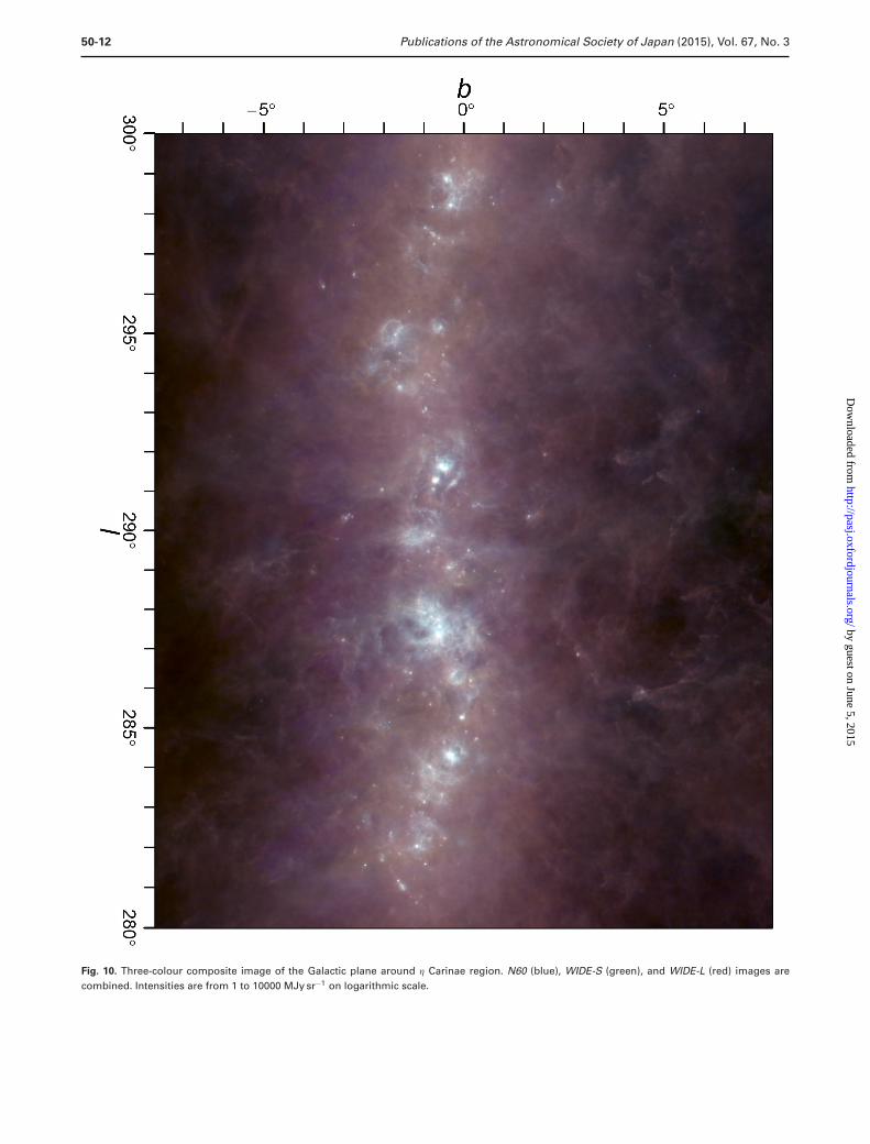
Fig. 10. Three-colour composite image of the Galactic plane around η Carinae region. N60 (blue), WIDE-S (green), and WIDE-L (red) images arecombined. Intensities are from 1 to 10000 MJy sr−1 on logarithmic scale.
by guest on June 5, 2015http://pasj.oxfordjournals.org/
Dow
nloaded from
Publications of the Astronomical Society of Japan (2015), Vol. 67, No. 3 50-13
indicates a tighter connection to the star-formation activityby tracing high ISRF regions at and around star-formingregions. The extended emission seen at longer wavelengthstraces spatial distribution of low-temperature dust in high-latitude cirrus clouds. This noticeable dependence of thespatial distribution on the wavelength difference between65 µm and 160 µm shows the importance of the wide wave-length coverage of AKARI to observe the FIR dust emissionat the peak of its SED where it has the largest dependenceon the temperature difference of the dust particles. This dif-ference in concentration at the Galactic plane is also visiblein a zoomed-in image of the Galactic plane at l = 280◦–300◦
(figure 10).The emission ranging from the tenuous dust in high
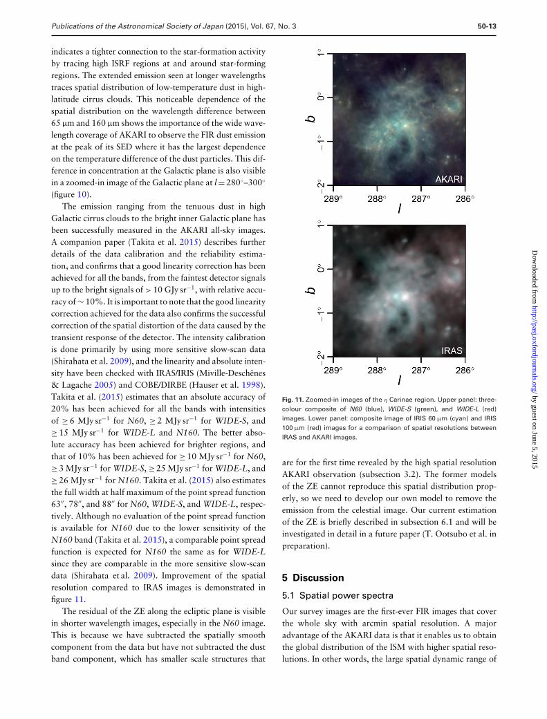
Galactic cirrus clouds to the bright inner Galactic plane hasbeen successfully measured in the AKARI all-sky images.A companion paper (Takita et al. 2015) describes furtherdetails of the data calibration and the reliability estima-tion, and confirms that a good linearity correction has beenachieved for all the bands, from the faintest detector signalsup to the bright signals of > 10 GJy sr−1, with relative accu-racy of ∼ 10%. It is important to note that the good linearitycorrection achieved for the data also confirms the successfulcorrection of the spatial distortion of the data caused by thetransient response of the detector. The intensity calibrationis done primarily by using more sensitive slow-scan data(Shirahata et al. 2009), and the linearity and absolute inten-sity have been checked with IRAS/IRIS (Miville-Deschenes& Lagache 2005) and COBE/DIRBE (Hauser et al. 1998).Takita et al. (2015) estimates that an absolute accuracy of20% has been achieved for all the bands with intensitiesof ≥ 6 MJy sr−1 for N60, ≥ 2 MJy sr−1 for WIDE-S, and≥ 15 MJy sr−1 for WIDE-L and N160. The better abso-lute accuracy has been achieved for brighter regions, andthat of 10% has been achieved for ≥ 10 MJy sr−1 for N60,≥ 3 MJy sr−1 for WIDE-S, ≥ 25 MJy sr−1 for WIDE-L, and≥ 26 MJy sr−1 for N160. Takita et al. (2015) also estimatesthe full width at half maximum of the point spread function63′′, 78′′, and 88′′ for N60, WIDE-S, and WIDE-L, respec-tively. Although no evaluation of the point spread functionis available for N160 due to the lower sensitivity of theN160 band (Takita et al. 2015), a comparable point spreadfunction is expected for N160 the same as for WIDE-Lsince they are comparable in the more sensitive slow-scandata (Shirahata et al. 2009). Improvement of the spatialresolution compared to IRAS images is demonstrated infigure 11.
The residual of the ZE along the ecliptic plane is visiblein shorter wavelength images, especially in the N60 image.This is because we have subtracted the spatially smoothcomponent from the data but have not subtracted the dustband component, which has smaller scale structures that
Fig. 11. Zoomed-in images of the η Carinae region. Upper panel: three-colour composite of N60 (blue), WIDE-S (green), and WIDE-L (red)images. Lower panel: composite image of IRIS 60 µm (cyan) and IRIS100 µm (red) images for a comparison of spatial resolutions betweenIRAS and AKARI images.
are for the first time revealed by the high spatial resolutionAKARI observation (subsection 3.2). The former modelsof the ZE cannot reproduce this spatial distribution prop-erly, so we need to develop our own model to remove theemission from the celestial image. Our current estimationof the ZE is briefly described in subsection 6.1 and will beinvestigated in detail in a future paper (T. Ootsubo et al. inpreparation).
5 Discussion
5.1 Spatial power spectra
Our survey images are the first-ever FIR images that coverthe whole sky with arcmin spatial resolution. A majoradvantage of the AKARI data is that it enables us to obtainthe global distribution of the ISM with higher spatial reso-lutions. In other words, the large spatial dynamic range of
by guest on June 5, 2015http://pasj.oxfordjournals.org/
Dow
nloaded from
50-14 Publications of the Astronomical Society of Japan (2015), Vol. 67, No. 3
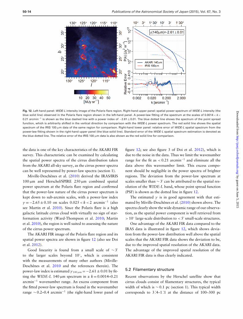
Fig. 12. Left-hand panel: WIDE-L intensity image of the Polaris flare region. Right-hand upper panel: spatial power spectrum of WIDE-L intensity (theblue solid line) observed in the Polaris flare region shown in the left-hand panel. A power-law fitting of the spectrum at the scales of 0.0014 < k <
0.21 arcmin−1 is shown as the blue dashed line with a power index of −2.61 ± 0.01. The blue dotted line shows the spectrum of the point spreadfunction, which is arbitrarily shifted in the vertical direction by comparison with the WIDE-L power spectrum. The red solid line shows the spatialspectrum of the IRIS 100 µm data of the same region for comparison. Right-hand lower panel: relative error of WIDE-L spatial spectrum from thepower-law fitting shown in the right-hand upper panel (the blue solid line). Standard error of the WIDE-L spatial spectrum estimation is denoted asthe blue dotted line. The relative error of the IRIS 100 µm data is also shown as the red solid line for comparison.
the data is one of the key characteristics of the AKARI FIRsurvey. This characteristic can be examined by calculatingthe spatial power spectra of the cirrus distribution takenfrom the AKARI all-sky survey, as the cirrus power spectracan be well represented by power-law spectra (section 1).
Miville-Deschenes et al. (2010) derived the IRAS/IRIS100 µm and Herschel/SPIRE 250 µm combined spatialpower spectrum at the Polaris flare region and confirmedthat the power-law nature of the cirrus power spectrum iskept down to sub-arcmin scales, with a power-law indexγ =−2.65 ± 0.10 on scales 0.025 < k < 2 arcmin−1 (alsosee Martin et al. 2010). Since the Polaris flare is a highgalactic latitude cirrus cloud with virtually no sign of star-formation activity (Ward-Thompson et al. 2010; Martinet al. 2010), the region is well suited to assessing the natureof the cirrus power spectrum.
The AKARI FIR image of the Polaris flare region and itsspatial power spectra are shown in figure 12 (also see Doiet al. 2012).
Good linearity is found from a small scale of ∼ 3′
to the larger scales beyond 10◦, which is consistentwith the measurements of many other authors (Miville-Deschenes et al. 2010 and the references therein). Thepower-law index is estimated γ 140 μm =−2.61 ± 0.01 by fit-ting the WIDE-L 140 µm spectrum in a k = 0.0014–0.21arcmin−1 wavenumber range. An excess component fromthe fitted power-law spectrum is found in the wavenumberrange ∼ 0.2–0.4 arcmin−1 (the right-hand lower panel of
figure 12; see also figure 3 of Doi et al. 2012), which isdue to the noise in the data. Thus we limit the wavenumberrange for the fit as < 0.21 arcmin−1 and eliminate all thedata above this wavenumber limit. This excess compo-nent should be negligible in the power spectra of brighterregions. The deviation from the power-law spectrum atscales smaller than ∼ 3′ can be attributed to the spatial res-olution of the WIDE-L band, whose point spread function(PSF) is shown as the dotted line in figure 12.
The estimated γ is in good agreement with that esti-mated by Miville-Deschenes et al. (2010) shown above. Thespectra clearly show the wide dynamic range of our observa-tion, as the spatial power component is well retrieved from> 10◦ large-scale distribution to < 5′ small-scale structures.
One advantage of the AKARI FIR data compared to theIRAS data is illustrated in figure 12, which shows devia-tion from the power-law distribution well above the spatialscales that the AKARI FIR data shows the deviation to be,due to the improved spatial resolution of the AKARI data.The advantage of the improved spatial resolution of theAKARI FIR data is thus clearly indicated.
5.2 Filamentary structure
Recent observations by the Herschel satellite show thatcirrus clouds consist of filamentary structures, the typicalwidth of which is ∼ 0.1 pc (section 1). This typical widthcorresponds to 3 .′4–1 .′1 at the distance of 100–300 pc
by guest on June 5, 2015http://pasj.oxfordjournals.org/
Dow
nloaded from
Publications of the Astronomical Society of Japan (2015), Vol. 67, No. 3 50-15
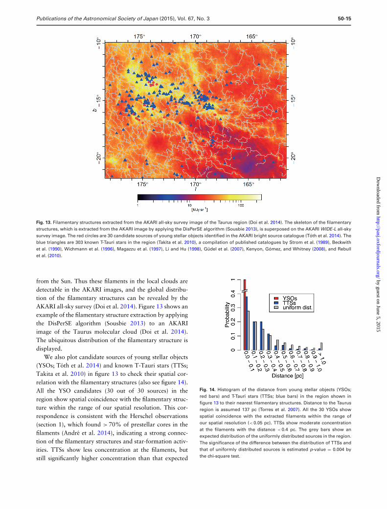
Fig. 13. Filamentary structures extracted from the AKARI all-sky survey image of the Taurus region (Doi et al. 2014). The skeleton of the filamentarystructures, which is extracted from the AKARI image by applying the DisPerSE algorithm (Sousbie 2013), is superposed on the AKARI WIDE-L all-skysurvey image. The red circles are 30 candidate sources of young stellar objects identified in the AKARI bright source catalogue (Toth et al. 2014). Theblue triangles are 303 known T-Tauri stars in the region (Takita et al. 2010), a compilation of published catalogues by Strom et al. (1989), Beckwithet al. (1990), Wichmann et al. (1996), Magazzu et al. (1997), Li and Hu (1998), Gudel et al. (2007), Kenyon, Gomez, and Whitney (2008), and Rebullet al. (2010).
from the Sun. Thus these filaments in the local clouds aredetectable in the AKARI images, and the global distribu-tion of the filamentary structures can be revealed by theAKARI all-sky survey (Doi et al. 2014). Figure 13 shows anexample of the filamentary structure extraction by applyingthe DisPerSE algorithm (Sousbie 2013) to an AKARIimage of the Taurus molecular cloud (Doi et al. 2014).The ubiquitous distribution of the filamentary structure isdisplayed.
We also plot candidate sources of young stellar objects(YSOs; Toth et al. 2014) and known T-Tauri stars (TTSs;Takita et al. 2010) in figure 13 to check their spatial cor-relation with the filamentary structures (also see figure 14).All the YSO candidates (30 out of 30 sources) in theregion show spatial coincidence with the filamentary struc-ture within the range of our spatial resolution. This cor-respondence is consistent with the Herschel observations(section 1), which found > 70% of prestellar cores in thefilaments (Andre et al. 2014), indicating a strong connec-tion of the filamentary structures and star-formation activ-ities. TTSs show less concentration at the filaments, butstill significantly higher concentration than that expected
Fig. 14. Histogram of the distance from young stellar objects (YSOs;red bars) and T-Tauri stars (TTSs; blue bars) in the region shown infigure 13 to their nearest filamentary structures. Distance to the Taurusregion is assumed 137 pc (Torres et al. 2007). All the 30 YSOs showspatial coincidence with the extracted filaments within the range ofour spatial resolution (< 0.05 pc). TTSs show moderate concentrationat the filaments with the distance < 0.4 pc. The grey bars show anexpected distribution of the uniformly distributed sources in the region.The significance of the difference between the distribution of TTSs andthat of uniformly distributed sources is estimated p-value = 0.004 bythe chi-square test.
by guest on June 5, 2015http://pasj.oxfordjournals.org/
Dow
nloaded from
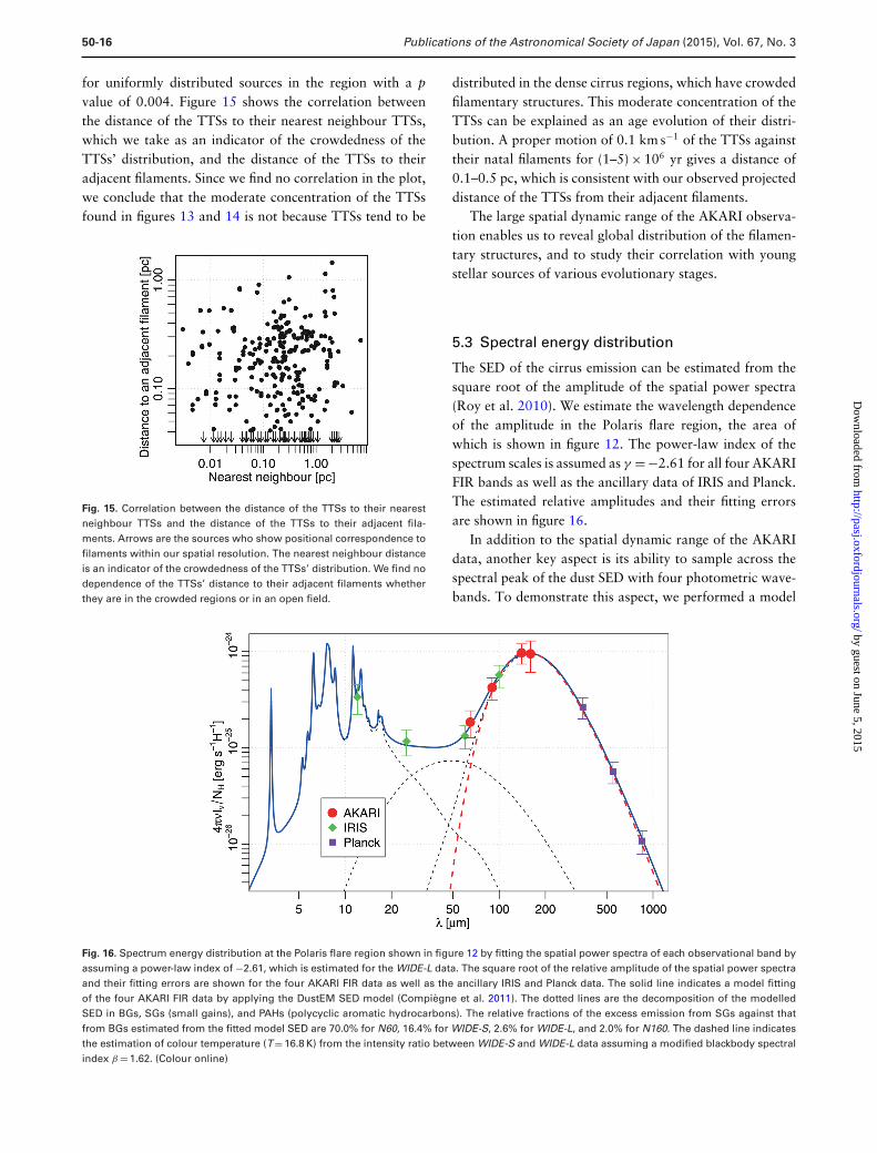
50-16 Publications of the Astronomical Society of Japan (2015), Vol. 67, No. 3
for uniformly distributed sources in the region with a pvalue of 0.004. Figure 15 shows the correlation betweenthe distance of the TTSs to their nearest neighbour TTSs,which we take as an indicator of the crowdedness of theTTSs’ distribution, and the distance of the TTSs to theiradjacent filaments. Since we find no correlation in the plot,we conclude that the moderate concentration of the TTSsfound in figures 13 and 14 is not because TTSs tend to be
Fig. 15. Correlation between the distance of the TTSs to their nearestneighbour TTSs and the distance of the TTSs to their adjacent fila-ments. Arrows are the sources who show positional correspondence tofilaments within our spatial resolution. The nearest neighbour distanceis an indicator of the crowdedness of the TTSs’ distribution. We find nodependence of the TTSs’ distance to their adjacent filaments whetherthey are in the crowded regions or in an open field.
distributed in the dense cirrus regions, which have crowdedfilamentary structures. This moderate concentration of theTTSs can be explained as an age evolution of their distri-bution. A proper motion of 0.1 km s−1 of the TTSs againsttheir natal filaments for (1–5) × 106 yr gives a distance of0.1–0.5 pc, which is consistent with our observed projecteddistance of the TTSs from their adjacent filaments.
The large spatial dynamic range of the AKARI observa-tion enables us to reveal global distribution of the filamen-tary structures, and to study their correlation with youngstellar sources of various evolutionary stages.
5.3 Spectral energy distribution
The SED of the cirrus emission can be estimated from thesquare root of the amplitude of the spatial power spectra(Roy et al. 2010). We estimate the wavelength dependenceof the amplitude in the Polaris flare region, the area ofwhich is shown in figure 12. The power-law index of thespectrum scales is assumed as γ =−2.61 for all four AKARIFIR bands as well as the ancillary data of IRIS and Planck.The estimated relative amplitudes and their fitting errorsare shown in figure 16.
In addition to the spatial dynamic range of the AKARIdata, another key aspect is its ability to sample across thespectral peak of the dust SED with four photometric wave-bands. To demonstrate this aspect, we performed a model
Fig. 16. Spectrum energy distribution at the Polaris flare region shown in figure 12 by fitting the spatial power spectra of each observational band byassuming a power-law index of −2.61, which is estimated for the WIDE-L data. The square root of the relative amplitude of the spatial power spectraand their fitting errors are shown for the four AKARI FIR data as well as the ancillary IRIS and Planck data. The solid line indicates a model fittingof the four AKARI FIR data by applying the DustEM SED model (Compiegne et al. 2011). The dotted lines are the decomposition of the modelledSED in BGs, SGs (small gains), and PAHs (polycyclic aromatic hydrocarbons). The relative fractions of the excess emission from SGs against thatfrom BGs estimated from the fitted model SED are 70.0% for N60, 16.4% for WIDE-S, 2.6% for WIDE-L, and 2.0% for N160. The dashed line indicatesthe estimation of colour temperature (T = 16.8 K) from the intensity ratio between WIDE-S and WIDE-L data assuming a modified blackbody spectralindex β = 1.62. (Colour online)
by guest on June 5, 2015http://pasj.oxfordjournals.org/
Dow
nloaded from
Publications of the Astronomical Society of Japan (2015), Vol. 67, No. 3 50-17
fit to the AKARI FIR data with the Compiegne et al. (2011)dust model, using the DustEM numerical tool,1 as indicatedin figure 16. It is clear that we can accurately reproduce theFIR dust SED with the AKARI FIR data, as the fitted modelSED agrees well with all the ancillary data.
The colour temperature from the WIDE-S/WIDE-Lintensity ratio (90 µm/140 µm) is estimated to beT = 16.8 K. A modified blackbody spectrum of the esti-mated temperature is shown in figure 16 as the dashed line.A modified blackbody spectral index is assumed β = 1.62,which is a mean value over the whole sky estimated byPlanck Collaboration (2014b) by fitting IRIS 100 µm andPlanck 353, 545, and 857 GHz data with modified black-body spectra. The estimated colour temperature spectrum isconsistent with the FIR–sub-mm part of the BGs’ emissionspectrum as well as the Planck observations.
The AKARI FIR data is therefore a good tracer of thetemperature, and of the total amount of BGs, and, as aresult, of the ISM as a whole. Together with the muchimproved spatial resolution from the former all-sky surveydata in the FIR wavebands, the newly achieved AKARI FIRhigh spatial resolution images of the whole sky should be apowerful tool for investigating the detailed spatial structureof ISM and its physical environment.
6 Caveats and plans for future
improvements
Although we have produced a sensitive all-sky FIR images,the data still contains some artefacts, and there is scopefor further improvements. In the following, we describeremaining caveats about the efficacy of the data and ourplans to mitigate these remaining problems.
6.1 Zodiacal emission
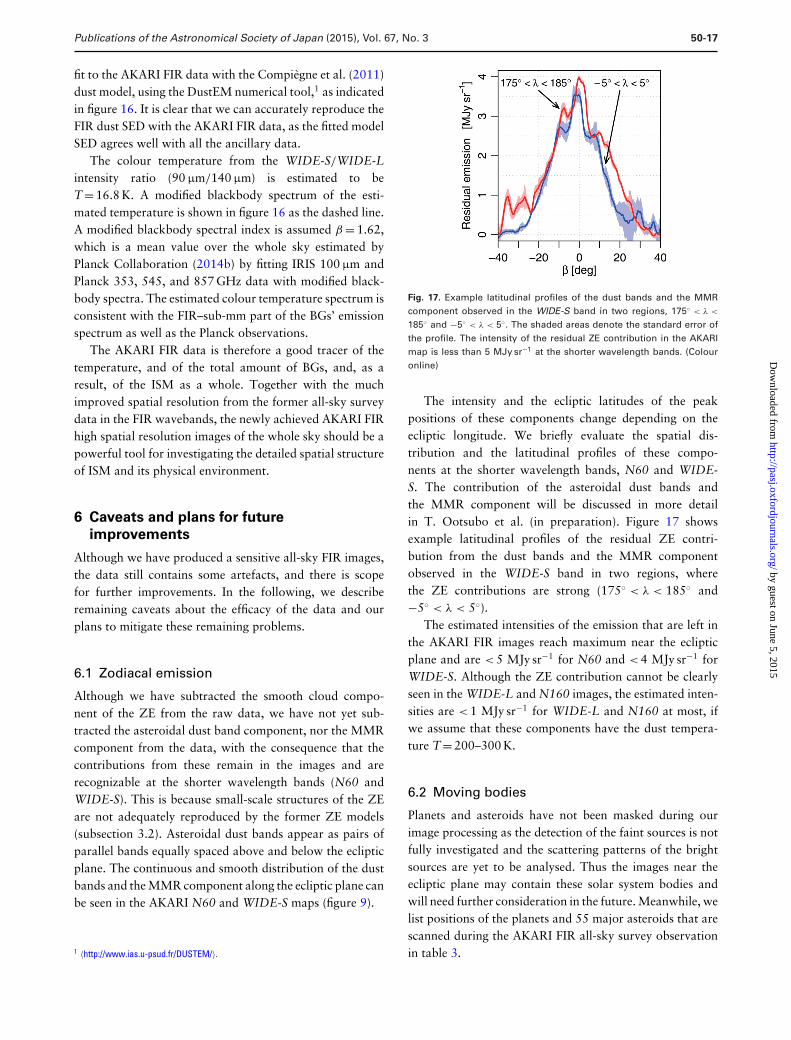
Although we have subtracted the smooth cloud compo-nent of the ZE from the raw data, we have not yet sub-tracted the asteroidal dust band component, nor the MMRcomponent from the data, with the consequence that thecontributions from these remain in the images and arerecognizable at the shorter wavelength bands (N60 andWIDE-S). This is because small-scale structures of the ZEare not adequately reproduced by the former ZE models(subsection 3.2). Asteroidal dust bands appear as pairs ofparallel bands equally spaced above and below the eclipticplane. The continuous and smooth distribution of the dustbands and the MMR component along the ecliptic plane canbe seen in the AKARI N60 and WIDE-S maps (figure 9).
1 〈http://www.ias.u-psud.fr/DUSTEM/〉.
Fig. 17. Example latitudinal profiles of the dust bands and the MMRcomponent observed in the WIDE-S band in two regions, 175◦ < λ <
185◦ and −5◦ < λ < 5◦. The shaded areas denote the standard error ofthe profile. The intensity of the residual ZE contribution in the AKARImap is less than 5 MJy sr−1 at the shorter wavelength bands. (Colouronline)
The intensity and the ecliptic latitudes of the peakpositions of these components change depending on theecliptic longitude. We briefly evaluate the spatial dis-tribution and the latitudinal profiles of these compo-nents at the shorter wavelength bands, N60 and WIDE-S. The contribution of the asteroidal dust bands andthe MMR component will be discussed in more detailin T. Ootsubo et al. (in preparation). Figure 17 showsexample latitudinal profiles of the residual ZE contri-bution from the dust bands and the MMR componentobserved in the WIDE-S band in two regions, wherethe ZE contributions are strong (175◦ < λ < 185◦ and−5◦ < λ < 5◦).
The estimated intensities of the emission that are left inthe AKARI FIR images reach maximum near the eclipticplane and are < 5 MJy sr−1 for N60 and < 4 MJy sr−1 forWIDE-S. Although the ZE contribution cannot be clearlyseen in the WIDE-L and N160 images, the estimated inten-sities are < 1 MJy sr−1 for WIDE-L and N160 at most, ifwe assume that these components have the dust tempera-ture T = 200–300 K.
6.2 Moving bodies
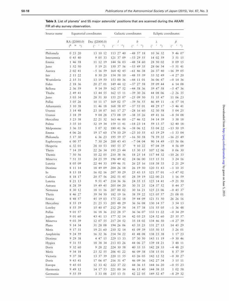
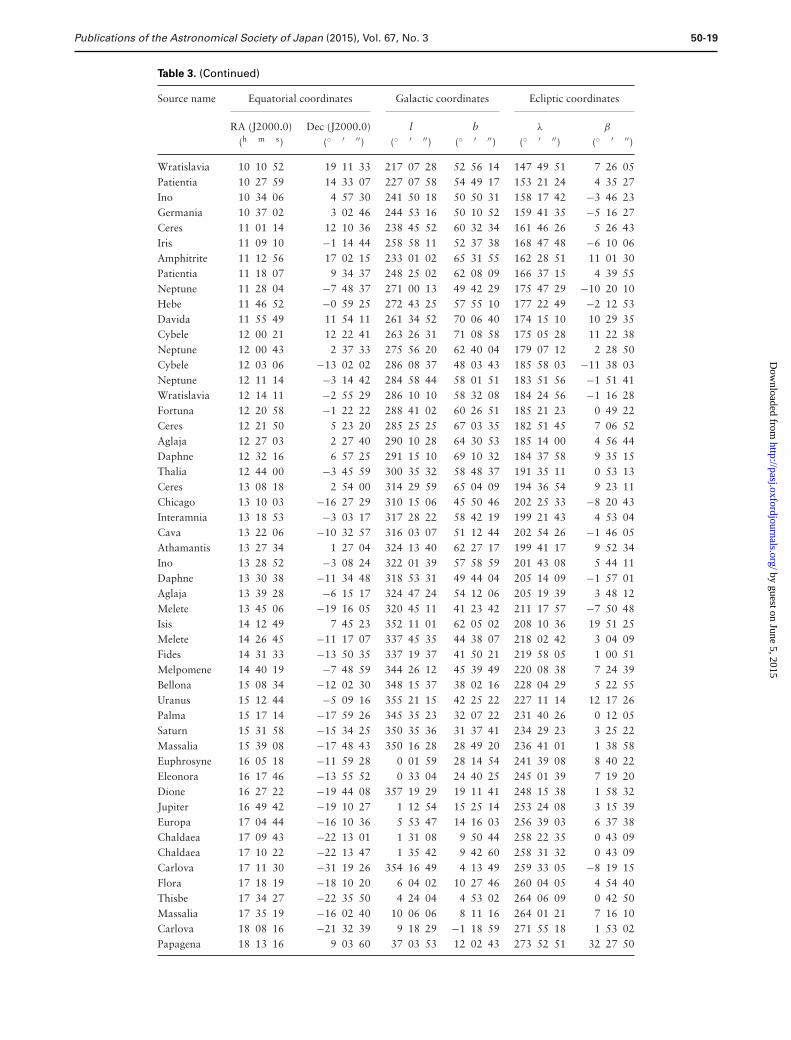
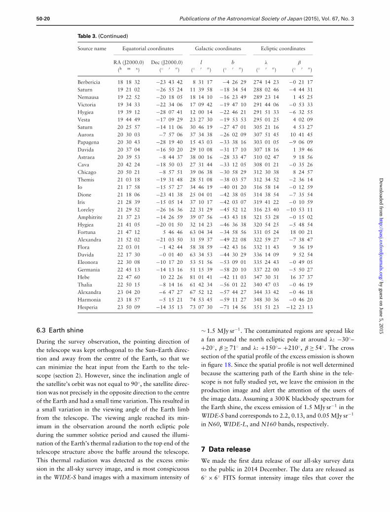
Planets and asteroids have not been masked during ourimage processing as the detection of the faint sources is notfully investigated and the scattering patterns of the brightsources are yet to be analysed. Thus the images near theecliptic plane may contain these solar system bodies andwill need further consideration in the future. Meanwhile, welist positions of the planets and 55 major asteroids that arescanned during the AKARI FIR all-sky survey observationin table 3.
by guest on June 5, 2015http://pasj.oxfordjournals.org/
Dow
nloaded from
50-18 Publications of the Astronomical Society of Japan (2015), Vol. 67, No. 3
Table 3. List of planets’ and 55 major asteroids’ positions that are scanned during the AKARI
FIR all-sky survey observation.
Source name Equatorial coordinates Galactic coordinates Ecliptic coordinates
RA (J2000.0) Dec (J2000.0) l b λ β
(h m s) (◦ ′ ′′) (◦ ′ ′′) (◦ ′ ′′) (◦ ′ ′′) (◦ ′ ′′)
Philomela 0 23 20 13 10 12 113 27 40 −48 57 18 10 36 32 9 46 07Interamnia 0 45 40 9 05 33 121 37 09 −53 29 55 14 02 59 3 51 15Emma 1 46 58 11 12 19 144 56 03 −48 54 60 28 50 02 0 09 15Juno 1 52 50 5 19 21 150 37 56 −53 49 35 28 06 34 −5 51 41Aurora 2 02 41 −5 16 59 164 42 45 −61 46 38 26 37 40 −16 39 05Isis 2 11 22 8 30 20 154 58 10 −48 55 39 33 32 49 −4 27 20Wratislavia 2 15 31 13 19 50 153 00 36 −44 11 01 36 06 47 −0 14 36Fides 2 18 36 20 27 01 149 44 12 −37 27 58 39 09 44 6 14 08Bellona 2 36 59 9 14 59 162 17 52 −44 58 36 39 47 58 −5 47 36Thisbe 2 49 41 13 44 55 162 15 11 −39 30 26 44 08 06 −2 26 35Juno 3 03 34 28 51 30 155 25 07 −25 09 50 51 35 47 11 06 23Pallas 3 05 26 10 11 17 169 02 57 −39 56 55 46 49 11 −6 57 14Athamantis 3 10 38 11 46 18 168 58 07 −37 55 01 48 29 17 −5 46 41Uranus 3 14 48 23 18 07 161 17 27 −28 16 60 52 30 58 5 04 25Uranus 3 18 39 9 04 28 173 08 19 −38 35 26 49 41 16 −8 54 08Herculina 3 23 38 22 21 32 163 46 00 −27 46 52 54 14 39 3 38 18Palma 3 35 10 32 19 34 159 11 41 −18 23 14 59 13 37 12 40 18Melpomene 3 36 35 5 07 32 180 41 56 −38 06 12 53 04 22 −13 50 19Emma 4 06 26 19 17 60 174 10 29 −23 10 55 63 19 29 −1 33 04Philomela 5 17 30 6 36 23 195 59 57 −16 50 58 78 59 35 −16 25 49Euphrosyne 6 00 57 7 30 24 200 43 43 −7 04 04 90 14 49 −15 56 06Hesperia 6 32 01 28 10 53 185 55 37 9 10 22 97 04 39 4 56 09Thetis 7 14 39 22 26 34 195 23 44 15 30 15 107 12 06 0 06 30Themis 7 50 56 10 22 05 210 38 56 18 25 14 117 44 32 −10 26 33Minerva 7 51 35 24 25 59 196 49 42 24 06 00 115 15 31 3 24 16Lutetia 8 05 09 22 44 33 199 46 51 26 25 16 118 38 33 2 21 29Diotima 8 11 14 18 49 09 204 26 18 26 19 50 120 51 43 −1 10 35Io 8 13 18 16 02 16 207 30 29 25 43 15 121 57 01 −3 47 02Callisto 8 18 17 20 57 56 202 51 45 28 39 19 122 00 21 1 16 59Lutetia 8 21 13 9 51 47 214 36 36 24 55 15 125 14 41 −9 21 50Astraea 8 28 39 19 49 45 205 04 20 30 31 25 124 37 52 0 44 37Nemausa 8 30 12 18 11 16 207 00 02 30 16 21 125 23 06 −0 45 37Thetis 8 46 27 39 54 50 182 19 16 38 59 22 123 05 57 21 08 01Emma 8 48 57 45 19 03 175 22 18 39 44 09 121 51 50 26 26 16Herculina 8 55 19 21 25 53 205 48 29 36 56 08 130 14 57 3 54 13Loreley 8 55 39 15 40 07 212 29 54 34 57 38 131 55 05 −1 36 48Pallas 9 01 57 16 18 36 212 28 57 36 36 07 133 11 22 −0 34 29Jupiter 9 01 60 43 41 13 177 32 14 42 03 25 124 52 60 25 35 57Minerva 9 03 39 12 07 55 217 24 52 35 18 02 134 46 50 −4 27 39Pluto 9 14 34 31 28 08 194 26 06 43 35 25 131 27 15 14 45 29Metis 9 17 31 19 21 60 210 32 14 41 09 39 135 50 15 3 26 01Amphitrite 9 24 59 16 32 36 214 54 22 41 48 08 138 23 38 1 17 23Diotima 9 29 38 4 47 15 229 13 33 37 30 50 143 11 19 −9 30 46Hygiea 9 31 55 18 38 34 213 03 26 44 06 27 139 18 21 3 48 11Doris 9 32 60 9 28 22 224 30 58 40 33 33 142 28 33 −4 48 25Metis 9 34 18 23 32 55 206 41 22 46 09 38 138 15 01 8 37 39Victoria 9 37 38 13 37 39 220 11 55 43 26 03 142 12 52 −0 30 27Doris 9 43 41 17 06 07 216 31 47 46 09 36 142 27 34 3 15 11Europa 9 45 03 12 33 42 222 37 22 44 36 15 144 16 20 −0 55 23Harmonia 9 49 12 14 17 53 221 00 34 46 15 40 144 38 35 1 02 58Germania 9 55 59 3 33 08 235 13 51 42 22 05 149 52 47 −8 29 32
by guest on June 5, 2015http://pasj.oxfordjournals.org/
Dow
nloaded from
Publications of the Astronomical Society of Japan (2015), Vol. 67, No. 3 50-19
Table 3. (Continued)
Source name Equatorial coordinates Galactic coordinates Ecliptic coordinates
RA (J2000.0) Dec (J2000.0) l b λ β
(h m s) (◦ ′ ′′) (◦ ′ ′′) (◦ ′ ′′) (◦ ′ ′′) (◦ ′ ′′)
Wratislavia 10 10 52 19 11 33 217 07 28 52 56 14 147 49 51 7 26 05Patientia 10 27 59 14 33 07 227 07 58 54 49 17 153 21 24 4 35 27Ino 10 34 06 4 57 30 241 50 18 50 50 31 158 17 42 −3 46 23Germania 10 37 02 3 02 46 244 53 16 50 10 52 159 41 35 −5 16 27Ceres 11 01 14 12 10 36 238 45 52 60 32 34 161 46 26 5 26 43Iris 11 09 10 −1 14 44 258 58 11 52 37 38 168 47 48 −6 10 06Amphitrite 11 12 56 17 02 15 233 01 02 65 31 55 162 28 51 11 01 30Patientia 11 18 07 9 34 37 248 25 02 62 08 09 166 37 15 4 39 55Neptune 11 28 04 −7 48 37 271 00 13 49 42 29 175 47 29 −10 20 10Hebe 11 46 52 −0 59 25 272 43 25 57 55 10 177 22 49 −2 12 53Davida 11 55 49 11 54 11 261 34 52 70 06 40 174 15 10 10 29 35Cybele 12 00 21 12 22 41 263 26 31 71 08 58 175 05 28 11 22 38Neptune 12 00 43 2 37 33 275 56 20 62 40 04 179 07 12 2 28 50Cybele 12 03 06 −13 02 02 286 08 37 48 03 43 185 58 03 −11 38 03Neptune 12 11 14 −3 14 42 284 58 44 58 01 51 183 51 56 −1 51 41Wratislavia 12 14 11 −2 55 29 286 10 10 58 32 08 184 24 56 −1 16 28Fortuna 12 20 58 −1 22 22 288 41 02 60 26 51 185 21 23 0 49 22Ceres 12 21 50 5 23 20 285 25 25 67 03 35 182 51 45 7 06 52Aglaja 12 27 03 2 27 40 290 10 28 64 30 53 185 14 00 4 56 44Daphne 12 32 16 6 57 25 291 15 10 69 10 32 184 37 58 9 35 15Thalia 12 44 00 −3 45 59 300 35 32 58 48 37 191 35 11 0 53 13Ceres 13 08 18 2 54 00 314 29 59 65 04 09 194 36 54 9 23 11Chicago 13 10 03 −16 27 29 310 15 06 45 50 46 202 25 33 −8 20 43Interamnia 13 18 53 −3 03 17 317 28 22 58 42 19 199 21 43 4 53 04Cava 13 22 06 −10 32 57 316 03 07 51 12 44 202 54 26 −1 46 05Athamantis 13 27 34 1 27 04 324 13 40 62 27 17 199 41 17 9 52 34Ino 13 28 52 −3 08 24 322 01 39 57 58 59 201 43 08 5 44 11Daphne 13 30 38 −11 34 48 318 53 31 49 44 04 205 14 09 −1 57 01Aglaja 13 39 28 −6 15 17 324 47 24 54 12 06 205 19 39 3 48 12Melete 13 45 06 −19 16 05 320 45 11 41 23 42 211 17 57 −7 50 48Isis 14 12 49 7 45 23 352 11 01 62 05 02 208 10 36 19 51 25Melete 14 26 45 −11 17 07 337 45 35 44 38 07 218 02 42 3 04 09Fides 14 31 33 −13 50 35 337 19 37 41 50 21 219 58 05 1 00 51Melpomene 14 40 19 −7 48 59 344 26 12 45 39 49 220 08 38 7 24 39Bellona 15 08 34 −12 02 30 348 15 37 38 02 16 228 04 29 5 22 55Uranus 15 12 44 −5 09 16 355 21 15 42 25 22 227 11 14 12 17 26Palma 15 17 14 −17 59 26 345 35 23 32 07 22 231 40 26 0 12 05Saturn 15 31 58 −15 34 25 350 35 36 31 37 41 234 29 23 3 25 22Massalia 15 39 08 −17 48 43 350 16 28 28 49 20 236 41 01 1 38 58Euphrosyne 16 05 18 −11 59 28 0 01 59 28 14 54 241 39 08 8 40 22Eleonora 16 17 46 −13 55 52 0 33 04 24 40 25 245 01 39 7 19 20Dione 16 27 22 −19 44 08 357 19 29 19 11 41 248 15 38 1 58 32Jupiter 16 49 42 −19 10 27 1 12 54 15 25 14 253 24 08 3 15 39Europa 17 04 44 −16 10 36 5 53 47 14 16 03 256 39 03 6 37 38Chaldaea 17 09 43 −22 13 01 1 31 08 9 50 44 258 22 35 0 43 09Chaldaea 17 10 22 −22 13 47 1 35 42 9 42 60 258 31 32 0 43 09Carlova 17 11 30 −31 19 26 354 16 49 4 13 49 259 33 05 −8 19 15Flora 17 18 19 −18 10 20 6 04 02 10 27 46 260 04 05 4 54 40Thisbe 17 34 27 −22 35 50 4 24 04 4 53 02 264 06 09 0 42 50Massalia 17 35 19 −16 02 40 10 06 06 8 11 16 264 01 21 7 16 10Carlova 18 08 16 −21 32 39 9 18 29 −1 18 59 271 55 18 1 53 02Papagena 18 13 16 9 03 60 37 03 53 12 02 43 273 52 51 32 27 50
by guest on June 5, 2015http://pasj.oxfordjournals.org/
Dow
nloaded from
50-20 Publications of the Astronomical Society of Japan (2015), Vol. 67, No. 3
Table 3. (Continued)
Source name Equatorial coordinates Galactic coordinates Ecliptic coordinates
RA (J2000.0) Dec (J2000.0) l b λ β
(h m s) (◦ ′ ′′) (◦ ′ ′′) (◦ ′ ′′) (◦ ′ ′′) (◦ ′ ′′)
Berbericia 18 18 32 −23 43 42 8 31 17 −4 26 29 274 14 23 −0 21 17Saturn 19 21 02 −26 55 24 11 39 58 −18 34 54 288 02 46 −4 44 31Nemausa 19 22 52 −20 18 05 18 14 10 −16 23 49 289 23 14 1 45 25Victoria 19 34 33 −22 34 06 17 09 42 −19 47 10 291 44 06 −0 53 33Hygiea 19 39 12 −28 07 41 12 00 14 −22 46 21 291 51 33 −6 32 55Vesta 19 44 49 −17 09 29 23 27 30 −19 53 53 295 01 25 4 02 09Saturn 20 25 57 −14 11 06 30 46 19 −27 47 01 305 21 16 4 53 27Aurora 20 30 03 −7 57 06 37 34 38 −26 02 09 307 51 45 10 41 45Papagena 20 30 43 −28 19 40 15 43 03 −33 38 16 303 01 05 −9 06 09Davida 20 37 04 −16 50 20 29 10 08 −31 17 10 307 18 16 1 39 46Astraea 20 39 53 −8 44 37 38 00 16 −28 33 47 310 02 47 9 18 56Cava 20 42 24 −18 50 03 27 31 44 −33 12 05 308 01 21 −0 35 26Chicago 20 50 21 −8 57 51 39 06 38 −30 58 29 312 30 38 8 24 57Themis 21 03 18 −19 31 48 28 51 08 −38 03 57 312 34 52 −2 36 14Io 21 17 58 −15 57 27 34 46 19 −40 01 20 316 58 14 −0 12 59Dione 21 18 06 −23 41 38 25 04 01 −42 38 05 314 38 54 −7 35 54Iris 21 28 39 −15 05 14 37 10 17 −42 03 07 319 41 22 −0 10 59Loreley 21 29 52 −26 16 36 22 31 29 −45 52 12 316 23 40 −10 53 11Amphitrite 21 37 23 −14 26 59 39 07 56 −43 43 18 321 53 28 −0 15 02Hygiea 21 41 05 −20 01 50 32 14 23 −46 36 38 320 54 25 −5 48 54Fortuna 21 47 12 5 46 46 63 04 34 −34 58 56 331 05 24 18 00 21Alexandra 21 52 02 −21 03 50 31 59 37 −49 22 08 322 59 27 −7 38 47Flora 22 03 01 −1 42 44 58 38 59 −42 43 16 332 11 43 9 36 19Davida 22 17 30 −0 01 40 63 34 53 −44 30 29 336 14 09 9 52 54Eleonora 22 30 08 −10 17 20 53 51 56 −53 09 01 335 24 43 −0 49 05Germania 22 45 13 −14 13 16 51 15 39 −58 20 10 337 22 00 −5 50 27Hebe 22 47 60 10 22 26 81 01 41 −42 11 03 347 30 31 16 37 37Thalia 22 50 15 −8 14 16 61 42 34 −56 01 22 340 47 03 −0 46 19Alexandra 23 04 20 −6 47 27 67 52 12 −57 44 27 344 33 42 −0 46 18Harmonia 23 18 57 −5 15 21 74 53 45 −59 11 27 348 30 36 −0 46 20Hesperia 23 50 09 −14 35 13 73 07 30 −71 14 56 351 51 23 −12 23 13
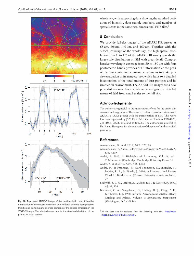
6.3 Earth shine
During the survey observation, the pointing direction ofthe telescope was kept orthogonal to the Sun–Earth direc-tion and away from the centre of the Earth, so that wecan minimize the heat input from the Earth to the tele-scope (section 2). However, since the inclination angle ofthe satellite’s orbit was not equal to 90◦, the satellite direc-tion was not precisely in the opposite direction to the centreof the Earth and had a small time variation. This resulted ina small variation in the viewing angle of the Earth limbfrom the telescope. The viewing angle reached its min-imum in the observation around the north ecliptic poleduring the summer solstice period and caused the illumi-nation of the Earth’s thermal radiation to the top end of thetelescope structure above the baffle around the telescope.This thermal radiation was detected as the excess emis-sion in the all-sky survey image, and is most conspicuousin the WIDE-S band images with a maximum intensity of
∼ 1.5 MJy sr−1. The contaminated regions are spread likea fan around the north ecliptic pole at around λ: −30◦–+20◦, β ≥ 71◦ and λ: +150◦– +210◦, β ≥ 54◦. The crosssection of the spatial profile of the excess emission is shownin figure 18. Since the spatial profile is not well determinedbecause the scattering path of the Earth shine in the tele-scope is not fully studied yet, we leave the emission in theproduction image and alert the attention of the users ofthe image data. Assuming a 300 K blackbody spectrum forthe Earth shine, the excess emission of 1.5 MJy sr−1 in theWIDE-S band corresponds to 2.2, 0.13, and 0.05 MJy sr−1
in N60, WIDE-L, and N160 bands, respectively.
7 Data release
We made the first data release of our all-sky survey datato the public in 2014 December. The data are released as6◦ × 6◦ FITS format intensity image tiles that cover the
by guest on June 5, 2015http://pasj.oxfordjournals.org/
Dow
nloaded from
Publications of the Astronomical Society of Japan (2015), Vol. 67, No. 3 50-21
Fig. 18. Top panel: WIDE-S image of the north ecliptic pole. A fan-likedistribution of the excess emission due to Earth shine is recognizable.Middle and bottom panels: cross sections of the excess emission in theWIDE-S image. The shaded areas denote the standard deviation of theprofile. (Colour online)
whole sky, with supporting data showing the standard devi-ation of intensity, data sample numbers, and number ofspatial scans in the same two-dimensional FITS files.2
8 Conclusion
We provide full-sky images of the AKARI FIR survey at65 µm, 90 µm, 140 µm, and 160 µm. Together with the> 99% coverage of the whole sky, the high spatial reso-lution from 1′ to 1 .′5 of the AKARI FIR survey reveals thelarge-scale distribution of ISM with great detail. Compre-hensive wavelength coverage from 50 to 180 µm with fourphotometric bands provides SED information at the peakof the dust continuum emission, enabling us to make pre-cise evaluation of its temperature, which leads to a detailedinvestigation of the total amount of dust particles and itsirradiation environment. The AKARI FIR images are a newpowerful resource from which we investigate the detailednature of ISM from small scales to the full sky.
Acknowledgments
The authors are grateful to the anonymous referee for the useful dis-cussions and suggestions. This research is based on observations withAKARI, a JAXA project with the participation of ESA. This workhas been supported by JSPS KAKENHI Grant Numbers 19204020,21111005, 25247016, and 25400220. The authors are grateful toDr. Sunao Hasegawa for the evaluation of the planets’ and asteroids’positions.
References
Arzoumanian, D., et al. 2011, A&A, 529, L6Arzoumanian, D., Andre, P., Peretto, N., & Konyves, V. 2013, A&A,
553, A119Andre, P. 2015, in Highlights of Astronomy, Vol. 16, ed.
T. Montmerle (Cambridge: Cambridge University Press), 31Andre, P., et al. 2010, A&A, 518, L102Andre, P., di Francesco, J., Ward-Thompson, D., Inutsuka, S.,
Pudritz, R. E., & Pineda, J. 2014, in Protostars and PlanetsVI, ed. H. Beuther et al. (Tucson: University of Arizona Press),27
Beckwith, S. V. W., Sargent, A. I., Chini, R. S., & Guesten, R. 1990,AJ, 99, 924
Beichman, C. A., Neugebauer, G., Habing, H. J., Clegg, P. E.,& Chester, T. J. 1988, Infrared Astronomical Satellite (IRAS)Catalogs and Atlases. Volume 1: Explanatory Supplement(Washington, D.C.: NASA)
2 All the data can be retrieved from the following web site: 〈http://www.ir.isas.jaxa.jp/ASTRO-F/Observation/〉.
by guest on June 5, 2015http://pasj.oxfordjournals.org/
Dow
nloaded from
50-22 Publications of the Astronomical Society of Japan (2015), Vol. 67, No. 3
Bernard, J. P., et al. 1999, A&A, 347, 640Bernard, J.-P., et al. 2010, A&A, 518, L88Berriman, G. B., Good, J. C., Laity, A. C., & Kong, M. 2008, in
ASP Conf. Ser., 394, Astronomical Data Analysis Software andSystems XVII, ed. R. W. Argyle et al. (San Francisco: ASP), 83
Boggess, N. W., et al. 1992, ApJ, 397, 420Boulanger, F., Abergel, A., Bernard, J.-P., Burton, W. B., Desert,
F.-X., Hartmann, D., Lagache, G., & Puget, J.-L. 1996, A&A,312, 256
Boulanger, F., & Perault, M. 1988, ApJ, 330, 964Compiegne, M., et al. 2011, A&A, 525, A103Compiegne, M., Flagey, N., Noriega-Crespo, A., Martin, P. G.,
Bernard, J.-P., Paladini, R., & Molinari, S. 2010, ApJ, 724, L44Desert, F.-X., Boulanger, F., & Puget, J. L. 1990, A&A, 237, 215Doi, Y., et al. 2009, ASP Conf. Ser., 418, 387Doi, Y., et al. 2012, Publ. Korean Astron. Soc., 27, 111Doi, Y., et al. 2014, Publi. Korean Astron. Soc., submittedDraine, B. T. 2003, ARA&A, 41, 241Draine, B. T., &, Li A. 2007, ApJ, 657, 810Gautier, T. N., Boulanger, F., III, Perault, M., & Puget, J. L. 1992,
AJ, 103, 1313Gorjian, V., Wright, E. L., & Chary, R. R. 2000, ApJ, 536, 550Gudel, M., et al. 2007, A&A, 468, 353Hauser, M.G., Kelsall, T., Leisawitz, D., & Weiland, J. ed.
1988, COBE Diffuse Infrared Background Experiment (DIRBE)Explanatory Supplement COBE Ref. Pub. No. 97-A (Greenbelt,MD: NASA/GSFC)
Jeong, W.-S., Mok Lee, H., Pak, S., Nakagawa, T., Minn Kwon, S.,Pearson, C. P., & White, G. J. 2005, MNRAS, 357, 535
Joncas, G., Boulanger, F., & Dewdney, P. E. 1992, ApJ, 397, 165Kaneda, H., et al. 2009, PASP, 121, 549Kawada, M., et al. 2007, PASJ, 59, S389Kelsall, T., et al. 1998, ApJ, 508, 44Kennicutt, R. C., Jr. 1998, ARA&A, 36, 189Kenyon, S. J., Gomez, M., & Whitney, B. A. 2008, Handbook of
Star Forming Regions, Volume I (San Francisco: ASP)Kiss, C., Abraham, P., Klaas, U., Juvela, M., & Lemke, D. 2001,
A&A, 379, 1161Kiss, C., Abraham, P., Klaas, U., Lemke, D., Heraudeau, P.,
del Burgo, C., & Herbstmeier, U. 2003, A&A, 399, 177Konyves, V., et al. 2010, A&A, 518, L106Lagache, G., Abergel, A., Boulanger, F., & Puget, J.-L. 1998, A&A,
333, 709Lagache, G., Haffner, L. M., Reynolds, R. J., & Tufte, S. L. 2000,
A&A, 354, 247Li, J. Z., & Hu, J. Y. 1998, A&AS, 132, 173Low, F. J., et al. 1984, ApJ, 278, L19Magazzu, A., Martin, E. L., Sterzik, M. F., Neuhauser, R.,
Covino, E., & Alcala, J. M. 1997, A&AS, 124, 449
Martin, P. G., et al. 2010, A&A, 518, L105Mathis, J. S. 1990, ARA&A, 28, 37Mathis, J. S., Mezger, P. G., & Panagia, N. 1983, A&A, 128,
212Meisner, A. M., & Finkbeiner, D. P. 2015, ApJ, 798, 88Miville-Deschenes, M.-A., et al. 2010, A&A, 518, L104Miville-Deschenes, M.-A., & Lagache, G. 2005, ApJS, 157, 302Miville-Deschenes, M.-A., Lagache, G., Boulanger, F., & Puget, J.-L.
2007, A&A, 469, 595Miville-Deschenes, M.-A., Lagache, G., & Puget, J.-L. 2002, A&A,
393, 749Murakami, H., et al. 2007, PASJ, 59, S369Nagata, H., Shibai, H., Hirao, T., Watabe, T., Noda, M.,
Hibi, Y., Kawada, M., & Nakagawa, T. 2004, IEEE Trans.Electron Devices, 51, 270
Nakagawa, T., et al. 2007, PASJ, 59, S377Neugebauer, G., et al. 1984, ApJ, 278, L1Onaka, T., et al. 2007, PASJ, 59, S401Pilbratt, G. L., et al. 2010, A&A, 518, L1Planck Commentoration 2011, A&A, 536, A19Planck Collaboration 2014a, A&A, 571, A1Planck Collaboration 2014b, A&A, 571, A11Planck Collaboration 2014c, arXiv:1409.2495Poglitsch, A., et al. 2010, A&A, 518, L2Pyo, J., et al. 2010, A&A, 523, A53Rebull, L. M., et al. 2010, ApJS, 186, 259Roy, A., et al. 2010, ApJ, 708, 1611Shirahata, M., et al. 2009, PASJ, 61, 737Schlegel, D. J., Finkbeiner, D. P., & Davis, M. 1998, ApJ, 500, 525Sousbie, T. 2013, Astrophysics Source Code Library, 1302.015
〈http://ascl.net/1302.015〉Strom, K. M., Strom, S. E., Edwards, S., Cabrit, S., & Skrutskie,
M. F. 1989, AJ, 97, 1451Suzuki, T., et al. 2008, PASP, 120, 895Takita, S., et al. 2015, PASJ, 67, 49Takita, S., Kataza, H., Kitamura, Y., Ishihara, D., Ita, Y., Oyabu, S.,
& Ueno, M. 2010, A&A, 519, A83Torres, R. M., Loinard, L., Mioduszewski, A. J., & Rodrıguez, L. F.
2007, ApJ, 671, 1813Toth, L. V., et al. 2014, PASJ, 66, 17Ward-Thompson, D., et al. 2010, A&A, 518, L92Wheelock, S. L., et al. 1994, IRAS Sky Survey Atlas: Explanatory
Supplement, NASA STI/Recon Technical Report No. 95-22539(Washington D.C.: NASA)
Wichmann, R., et al. 1996, A&A, 312, 439Wright, E. L. 1998, ApJ, 496, 1Yamamura, I., et al. 2009, in ASP Conf. Ser. 418, AKARI, a Light to
Illuminate the Misty Universe, ed. T. Onaka et al. (San Francisco:ASP), 3
by guest on June 5, 2015http://pasj.oxfordjournals.org/
Dow
nloaded from