The Calibration System for the Gerda Experiment DBD GERDA Calibration System Outlook The Calibration System for the Gerda Experiment Francis Froborg Universit at Z urich Doktorandenseminar

ν & DBD GERDA Calibration System Outlook

The Calibration System for the GerdaExperiment

Francis Froborg

Universitat Zurich

Doktorandenseminar30. August 2010

Francis Froborg Calibration of Gerda


Neutrino Physics

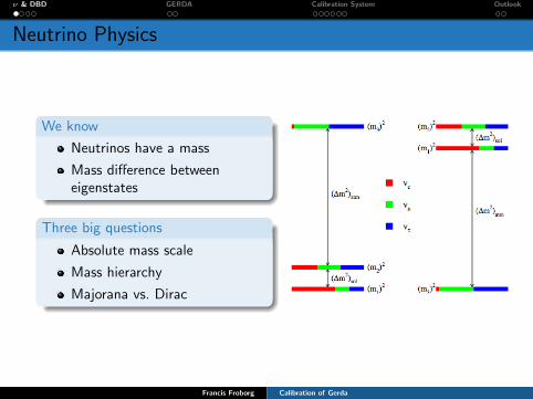
We know

Neutrinos have a mass

Mass difference betweeneigenstates

Three big questions

Absolute mass scale

Mass hierarchy

Majorana vs. Dirac



Double Beta Decay

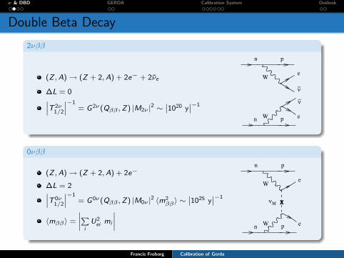
2νββ

(Z ,A)→ (Z + 2,A) + 2e− + 2νe

∆L = 0˛T 2ν

1/2

˛−1= G2ν(Qββ ,Z) |M2ν |2 ∼

˛1020 y

˛−1

3

!"

"

n

n p

p

e

e

!

W

W

"#

n

n p

p

e

eW

W

x

FIG. 2 Feynman Diagrams for !!(2") (left) and !!(0")(right).

where G0!(Q"" , Z) is the phase space factor for the emis-sion of the two electrons, M0! is another nuclear matrixelement, and !m""" is the “e!ective” Majorana mass ofthe electron neutrino:

!m""" # |!

k

mkU2ek| . (3)

Here the mk’s are the masses of the three light neutrinosand U is the matrix that transforms states with well-defined mass into states with well-defined flavor (e.g.,electron, mu, tau). Equation 2 gives the !!(0") rateif the exchange of light Majorana neutrinos with lefthanded interactions is responsible. Other mechanismsare possible (see Sections III and IV.D), but they requirethe existence of new particles and/or interactions in ad-dition to requiring that neutrinos be Majorana particles.Light-neutrino exchange is therefore, in some sense, the“minima” mechanism and the most commonly consid-ered.

That neutrinos mix and have mass is now acceptedwisdom. Oscillation experiments constrain U fairly well

— Table I summarizes our current knowledge — but theydetermine only the di!erences between the squares of themasses mk (e.g., m2

2 $m21) rather than the masses them-

selves. It will turn out that !!(0") is among the bestways of getting at the masses (along with cosmology and!-decay measurements), and the only practical way toestablish that neutrinos are Majorana particles.

To extract the e!ective mass from a measurement, itis customary to define a nuclear structure factor FN #G0!(Q"" , Z)|M0! |2m2

e, where me is the electron mass.(The quantity FN is sometimes written as Cmm.) Thee!ective mass !m""" can be written in terms of the cal-culated FN and the measured half life as

!m""" = me[FNT 0!1/2]

!1/2 . (4)

The range of mixing matrix values given below in Ta-ble I, combined with calculated values for FN , allow usto estimate the half-life a given experiment must be ableto measure in order to be sensitive to a particular valueof !m""". Published values of FN are typically between10!13 and 10!14 y!1. To reach a sensitivity of !m"""%0.1 eV, therefore, an experiment must be able to observea half life of 1026 $ 1027 y. As we discuss later, at thislevel of sensitivity an experiment can draw importantconclusions whether or not the decay is observed.

The most sensitive limits thus far are from theHeidelberg-Moscow experiment: T 0!

1/2(76Ge) & 1.9 '

1025 y (Baudis et al., 1999), the IGEX experiment:T 0!

1/2(76Ge) & 1.6 ' 1025 y (Aalseth et al., 2002a, 2004),

and the CUORICINO experiment T 0!1/2(

130Te) & 3.0 '1024 y (Arnaboldi et al., 2005, 2007). These experimentscontained 5 to 10 kg of the parent isotope and ran forseveral years. Hence, increasing the half-life sensitivityby a factor of about 100, the goal of the next generationof experiments, will require hundreds of kg of parent iso-tope and a significant decrease in background beyond thepresent state of the art (roughly 0.1 counts/(keV kg y).

It is straightforward to derive an approximate an-alytical expression for the half-life to which an ex-periment with a given level of background is sensi-tive (Avignone et al., 2005):

T 0!1/2(n#) =

4.16 ' 1026y

n#

" #a

W

#

$

Mt

b"(E). (5)

Here n# is the number of standard deviations correspond-ing to a given confidence level (C.L.) — a CL of 99.73%corresponds to n# = 3 — the quantity # is the event-detection and identification e#ciency, a is the isotopicabundance, W is the molecular weight of the source ma-terial, and M is the total mass of the source. The in-strumental spectral-width "(E), defining the signal re-gion, is related to the energy resolution at the energyof the expected !!(0") peak, and b is the specific back-ground rate in counts/(keV kg y), where the mass is that

0νββ

(Z ,A)→ (Z + 2,A) + 2e−

∆L = 2˛T 0ν

1/2

˛−1= G0ν(Qββ ,Z) |M0ν |2 〈m2

ββ〉 ∼˛1025 y

˛−1

〈mββ〉 =

˛Pi

U2ei mi

˛

3

!"

"

n

n p

p

e

e

!

W

W

"#

n

n p

p

e

eW

W

x

FIG. 2 Feynman Diagrams for !!(2") (left) and !!(0")(right).

where G0!(Q"" , Z) is the phase space factor for the emis-sion of the two electrons, M0! is another nuclear matrixelement, and !m""" is the “e!ective” Majorana mass ofthe electron neutrino:

!m""" # |!

k

mkU2ek| . (3)

Here the mk’s are the masses of the three light neutrinosand U is the matrix that transforms states with well-defined mass into states with well-defined flavor (e.g.,electron, mu, tau). Equation 2 gives the !!(0") rateif the exchange of light Majorana neutrinos with lefthanded interactions is responsible. Other mechanismsare possible (see Sections III and IV.D), but they requirethe existence of new particles and/or interactions in ad-dition to requiring that neutrinos be Majorana particles.Light-neutrino exchange is therefore, in some sense, the“minima” mechanism and the most commonly consid-ered.

That neutrinos mix and have mass is now acceptedwisdom. Oscillation experiments constrain U fairly well

— Table I summarizes our current knowledge — but theydetermine only the di!erences between the squares of themasses mk (e.g., m2

2 $m21) rather than the masses them-

selves. It will turn out that !!(0") is among the bestways of getting at the masses (along with cosmology and!-decay measurements), and the only practical way toestablish that neutrinos are Majorana particles.

To extract the e!ective mass from a measurement, itis customary to define a nuclear structure factor FN #G0!(Q"" , Z)|M0! |2m2

e, where me is the electron mass.(The quantity FN is sometimes written as Cmm.) Thee!ective mass !m""" can be written in terms of the cal-culated FN and the measured half life as

!m""" = me[FNT 0!1/2]

!1/2 . (4)

The range of mixing matrix values given below in Ta-ble I, combined with calculated values for FN , allow usto estimate the half-life a given experiment must be ableto measure in order to be sensitive to a particular valueof !m""". Published values of FN are typically between10!13 and 10!14 y!1. To reach a sensitivity of !m"""%0.1 eV, therefore, an experiment must be able to observea half life of 1026 $ 1027 y. As we discuss later, at thislevel of sensitivity an experiment can draw importantconclusions whether or not the decay is observed.

The most sensitive limits thus far are from theHeidelberg-Moscow experiment: T 0!

1/2(76Ge) & 1.9 '

1025 y (Baudis et al., 1999), the IGEX experiment:T 0!

1/2(76Ge) & 1.6 ' 1025 y (Aalseth et al., 2002a, 2004),

and the CUORICINO experiment T 0!1/2(

130Te) & 3.0 '1024 y (Arnaboldi et al., 2005, 2007). These experimentscontained 5 to 10 kg of the parent isotope and ran forseveral years. Hence, increasing the half-life sensitivityby a factor of about 100, the goal of the next generationof experiments, will require hundreds of kg of parent iso-tope and a significant decrease in background beyond thepresent state of the art (roughly 0.1 counts/(keV kg y).

It is straightforward to derive an approximate an-alytical expression for the half-life to which an ex-periment with a given level of background is sensi-tive (Avignone et al., 2005):

T 0!1/2(n#) =

4.16 ' 1026y

n#

" #a

W

#

$

Mt

b"(E). (5)

Here n# is the number of standard deviations correspond-ing to a given confidence level (C.L.) — a CL of 99.73%corresponds to n# = 3 — the quantity # is the event-detection and identification e#ciency, a is the isotopicabundance, W is the molecular weight of the source ma-terial, and M is the total mass of the source. The in-strumental spectral-width "(E), defining the signal re-gion, is related to the energy resolution at the energyof the expected !!(0") peak, and b is the specific back-ground rate in counts/(keV kg y), where the mass is that



Signature

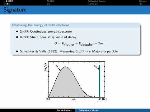
Measuring the energy of both electrons

2νββ: Continuous energy spectrum

0νββ: Sharp peak at Q value of decay

Q = Emother − Edaugther − 2me

Schechter & Valle (1982): Measuring 0νββ ⇒ ν Majorana particle



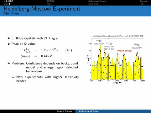
Heidelberg-Moscow ExperimentThe Claim

5 HPGe crystals with 71.7 kg y

Peak at Q value:

T 0ν1/2 = 1.2× 1025y (4σ)

〈mββ〉 = 0.44 eV

Problem: Confidence depends on backgroundmodel and energy region selectedfor analysis

⇒ New experiments with higher sensitivityneeded

Evidenz für den Neutrinolosen Doppelbetazerfall?

• Peak beim Q-Wert des Zerfalls

• Periode 1990-2003: 28.8 ± 6.9 Ereignisse

• Periode 1995-2003: 23.0 ± 5.7 Ereignisse

! 4.1- 4.2 ! Evidenz

• ‘Evidenz’ unklar

! muss mit neuen, empfindlicheren Experimenten getestet werden

T1/2

0!= 1.2 "10

25yr

214Bi2010.7 keV 214Bi

2016.2 keV

2021.8 keV

214Bi2052.9 keV

0nußß decay?

?

H.V.Klapdor-Kleingrothaus et al., Phys. Lett. B 586 (2004) 198

m!e = 0.44 eV (0.3"1.24) eV



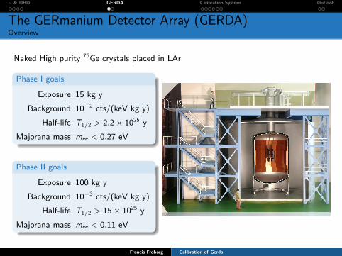
The GERmanium Detector Array (GERDA)Overview

Naked High purity 76Ge crystals placed in LAr

Phase I goals

Exposure 15 kg y

Background 10−2 cts/(keV kg y)

Half-life T1/2 > 2.2× 1025 y

Majorana mass mee < 0.27 eV

Phase II goals

Exposure 100 kg y

Background 10−3 cts/(keV kg y)

Half-life T1/2 > 15× 1025 y

Majorana mass mee < 0.11 eV



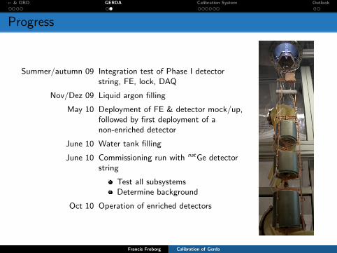
Progress

Summer/autumn 09 Integration test of Phase I detectorstring, FE, lock, DAQ

Nov/Dez 09 Liquid argon filling

May 10 Deployment of FE & detector mock/up,followed by first deployment of anon-enriched detector

June 10 Water tank filling

June 10 Commissioning run with natGe detectorstring

Test all subsystemsDetermine background

Oct 10 Operation of enriched detectors



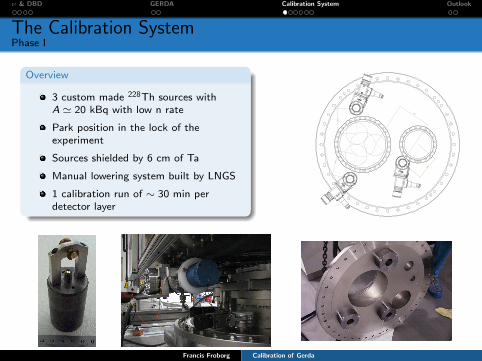
The Calibration SystemPhase I

Overview

3 custom made 228Th sources withA ' 20 kBq with low n rate

Park position in the lock of theexperiment

Sources shielded by 6 cm of Ta

Manual lowering system built by LNGS

1 calibration run of ∼ 30 min perdetector layer

62

14

274

138

135

178

130

17.11.2009

Blatt-Nr.:

Spez.:

. -???.1 1

Dateiname : J:\116.GERDA\014.CLUSTER Flansch\116014-Clusterflansch|Format : A0| Blatt 1 von 1 | Geändert durch: kbgp

???

1:5

Dienstag, 17. November 2009 15:17:26

Allgemeintoleranz DIN ISO 2768-mK

Bemerkung:

Zeichn.-Nr.: Zeichn.-Paket:

Zeichnung unterliegt nicht dem Änderungsdienst

Konstruktion

Datum der letzten Änderung

Werkstoff:

Benennung:

Abschnitt:

Projekt:

Anzahl:Maßstab:

Abschnitt-Nr.:

Projekt-Nr.:

Zeichner:

Konstukteur:

Koordinator:

Erstellt am:

Auftraggeber:Max-Planck-Institut

für KernphysikHeidelberg

Zentrale

Kanten ISO 13715

!"##$%"&'()*+,-.'/012.'!,3$"*%3&'45'24)-3,'6*&,-#%4*'27&#,8'19:;<'!,,#%*=';-,&>,*'?@AB?'()C7'BD?D

!"#$%&'()*+,#%#-'".,)#+

! /.+*)+*%,'(,%)+%/.00%1%2"'-#",'&%34%!".+5)(%#+%6789%$'',)+*:%;%<=

! >'$#?.0%#@%4'00#A%5#0#"%"'?'.0(%?'"4%-##"%$',.0%BC.0),4%;%)+5#D'"'+,%@)0$%.0A.4(%-"'('+,%;%+#,%(C),.30'%@#"%#C"%-C"-#('E

! FG5D.+*'&%$','"%3.+&%A),D%$',.0%A)"'%@"#$%H','"%I")?'%-"#?)&'&%34%JK/%;%$#&)@)5.,)#+%#@%(#$'%$'5D.+)5.0%&',.)0(%;%+'A%0#.&%,'(,(%)+%A#"L%(D#-%.+&%)+%/.00%1E%

! 6'.L%,'(,%-")#"%,#%)+(,.00.,)#+%;%0'.L%".,'%+,%(.,)(@.5,#"4%2A#"('%,D.+%M%MNOP$3."%0Q(E%;%)&'+,)@)'&%0'.L(%.+&%50#('&%-"#?)()#+.004%A),D%3)O5#$-#+'+,%*0C'%2HRSO/I:%;%0'.L%".,'%#@%M%MNET%$3."%0Q(E

! RC,%)+%#-'".,)#+%(D#",04%.@,'"%&'-0#4)+*%@)"(,%&','5,#"E



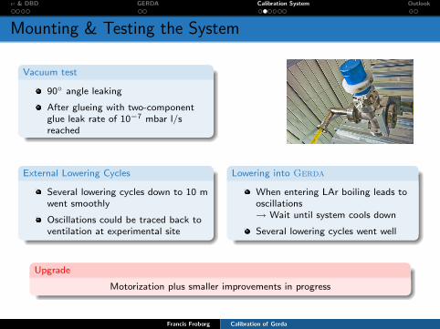
Mounting & Testing the System

Vacuum test

90◦ angle leaking

After glueing with two-componentglue leak rate of 10−7 mbar l/sreached

External Lowering Cycles

Several lowering cycles down to 10 mwent smoothly

Oscillations could be traced back toventilation at experimental site

Lowering into Gerda

When entering LAr boiling leads tooscillations→ Wait until system cools down

Several lowering cycles went well

Upgrade

Motorization plus smaller improvements in progress



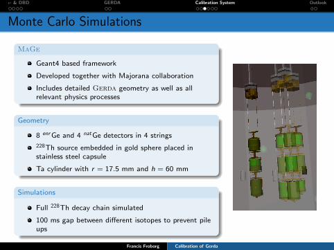
Monte Carlo Simulations

MaGe

Geant4 based framework

Developed together with Majorana collaboration

Includes detailed Gerda geometry as well as allrelevant physics processes

Geometry

8 enr Ge and 4 natGe detectors in 4 strings

228Th source embedded in gold sphere placed instainless steel capsule

Ta cylinder with r = 17.5 mm and h = 60 mm

Simulations

Full 228Th decay chain simulated

100 ms gap between different isotopes to prevent pileups



γ Background

Linear Attenuation

Take flux of sources in 1 year

Flux reduction because detector covers just small area but source radiatesisotropically

γ with highest energies have 2.6 MeV (36%)

Calculate linear attenuation of 250 cm of LAr and 6 cm of Ta absorber

Monte Carlo Simulation

Photon beam downwards 1m above detector array

Rescale hits in ROI to flux calculated above

Result for 3 20kBq sources

Bγ = 0.3× 10−5 cts/(keV kg y)



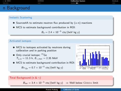
n Background

Inelastic Scattering

Sources4A to estimate neutron flux produced by (α-n) reactions

MCS to estimate background contribution in ROI:

Bn = 2.4× 10−5 cts/(keV kg y)

Activated isotopes

MCS to isotopes activated by neutrons duringcalibration and in parking position

Only crucial isotope: 77GeT1/2 = 11.3 h, Eγ,max = 2.35 MeV

MCS to estimate background contribution in ROI:

B77Ge = 0.7× 10−5 cts/(keV kg y)

Total Background (n & γ)

Btot = 3.4× 10−5 cts/(keV kg y) ⇒ Well below Gerda limit



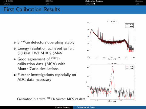
First Calibration Results

3 natGe detectors operating stably

Energy resolution achieved so far:3.8 keV FWHM @ 2.6MeV

Good agreement of 228Thcalibration data (MCA) withMonte Carlo simulations

Further investigations especially onADC data necessary

Calibration run with 228Th source: MCS vs data



OutlookData Analysis

Energy Calibration

Compare data with MCS

Test and optimize different energy reconstruction algorithms⇒ Important to achieve best possible energy resolution

⇒ T 0ν1/2 ∝ 〈mββ〉−2 ∝ const

√M×t

∆E×B

Pulse Shape Analysis

Distinguish between single-site and multi-site events⇒ Background reduction

Test different sets of parameters to determine optimal procedure



Summary

Calibration system installed and tested successfully

Upgrade on its way

Background contribution from calibration sources withB = 3.4× 10−5 cts/(keV kg y) well below Gerda limit

First data taken with natGe detectors in good agreement with MCSenr Ge detectors will be submerged in Oct

Future work will focus on data analysis


Documents

The Calibration System for the Gerda Experiment DBD GERDA Calibration System Outlook The Calibration System for the Gerda Experiment Francis Froborg Universit at Z urich Doktorandenseminar