FYSA21 Mathematical Tools in Science

The continuous and discrete Fourier transforms

Lennart LindegrenLund Observatory (Department of Astronomy, Lund University)

1 The continuous Fourier transform

1.1 Definitions

Provided that the integrals exist, the following holds:

f(ξ) =∫ +∞

−∞f(x) e−ixξ dx

f(x) =1

2π

∫ +∞

−∞f(ξ) eixξ dξ

(1)

The top equation defines the Fourier transform (FT) of the function f , the bottomequation defines the inverse Fourier transform of f . f and f are in general com-plex functions (see Sect. 1.3). The Fourier transform is sometimes denoted by theoperator F and its inverse by F−1, so that:

f = F [f ] , f = F−1[f ] (2)

It should be noted that the definitions in Eq. (1) are not the only ones found in theliterature. Examples of other conventions are given below.

Example 1: An alternative definition is

X(ω) =1√2π

∫ +∞

−∞x(t) eiωt dt

x(t) =1√2π

∫ +∞

−∞X(ω) e−iωt dω

(3)

Note the placement of the minus sign in the inverse transform, the use of the nor-malizing factor (2π)−1/2 on both integrals, and the notation using lower and uppercase letters for the function and its transform.

Example 2: Another common variant is

H(f) =∫ +∞

−∞h(t) ei2πft dt

h(t) =∫ +∞

−∞H(f) e−i2πft df

(4)

where the need for a normalization factor is eliminated by the substitution ω = 2πf .

1

The different definitions above are related by trivial substitution or scaling of thevariables. It is however important to know which definition is used in a particularapplication. The special case of x = 0 (or t = 0) and ξ = 0 (or ω = 0) are oftenuseful “test cases”; e.g., Eq. (1) gives:

f(0) =∫ +∞

−∞f(x) dx , f(0) =

1

2π

∫ +∞

−∞f(ξ) dξ (5)

1.2 Interpretation of the variables. Units

The variable x in Eq. (1) often represents length (i.e., a spatial coordinate) ellertime. The variable ξ should then be interpreted as wave number (spatial frequency)or angular frequency ; thus ξ = 2π/P , where P is the period in length or time.

If x is measured in [m], then ξ will be expressed in [rad m−1]. If x is measured in[s], then ξ will be expressed in [rad s−1]. When time is involved, the variables areusually denoted t and ω rather than x and ξ.

In Example 2, f stands for the “ordinary” frequency expressed in periods per unitof t; e.g., if t is length in [m], then f is spatial frequency in [per m−1] or [m−1]. If tis time in [s], then f is temporal frequency in [per s−1] or [Hz].

1.3 The FT of a real function

The definitions in Sect. 1.1 are valid for complex functions f and f . When f(x)represents a measured quantity it is usually real, in which case

f(−ξ) = f ∗(ξ) (real f) (6)

f is in general still complex, but its real part is even and its imaginary part odd. Iff(x) is real and even [so that f(−x) = f(x)], then f is also real and even. Figures 1–4show some Fourier transform pairs for real, even functions.

A general property of Fourier transform pairs is that a “wide” function has a “nar-row” FT, and vice versa. This localization property implies that we cannot arbitrar-ily concentrate both the function and its Fourier transform. This is illustrated inFigs. 1–4:• In Fig. 1 the boxcar function of width 2a is transformed into a sinc-function1

of width π/a (as measured from the centre to the first zero).

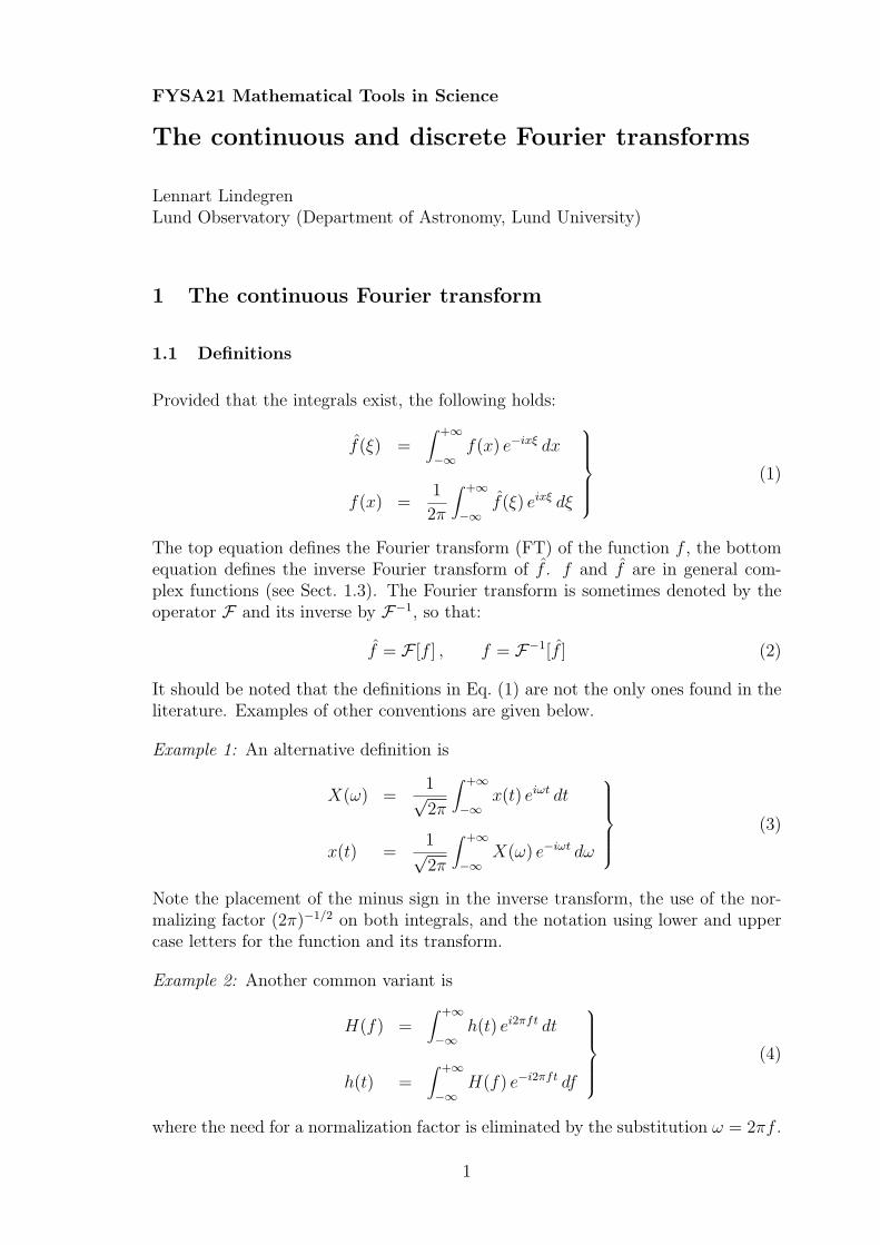
• In Fig. 2 a constant (being infinitely wide) is transformed into the (infinitelynarrow) delta function.2

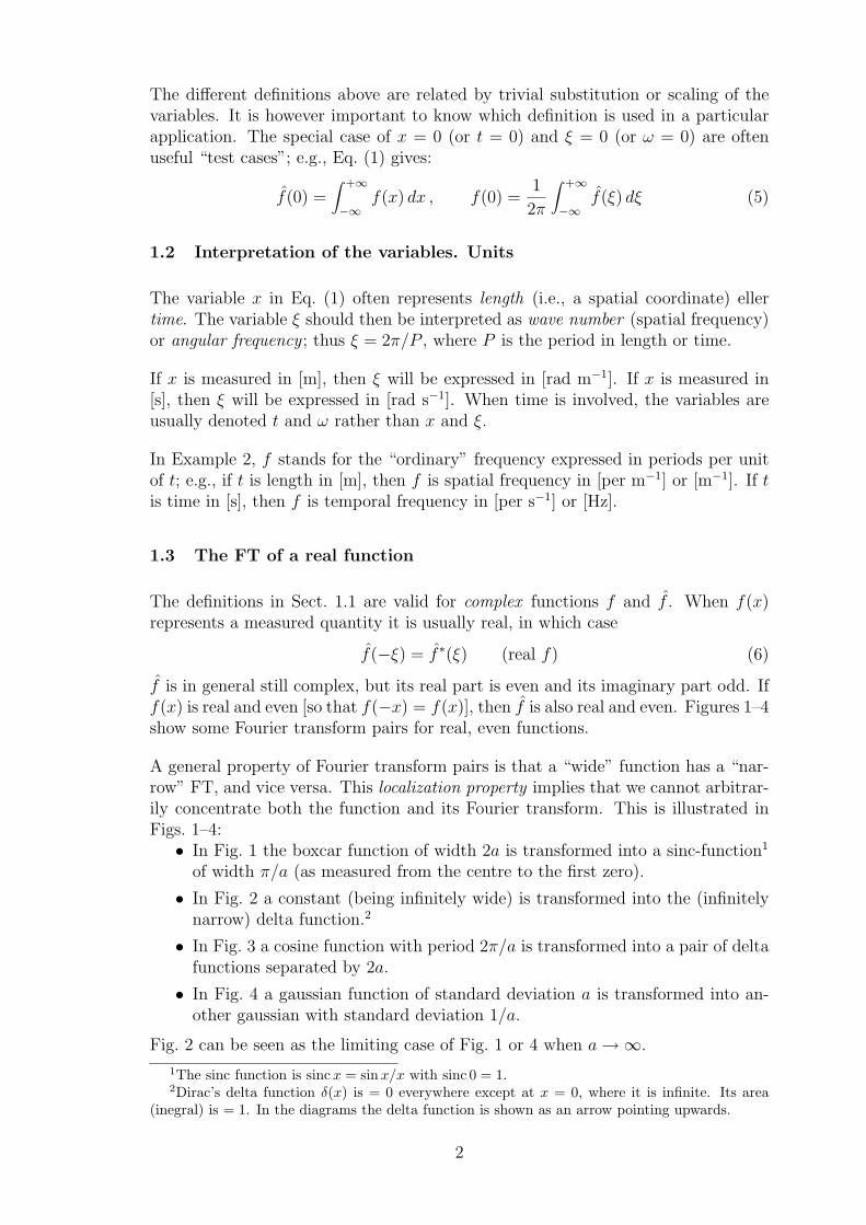
• In Fig. 3 a cosine function with period 2π/a is transformed into a pair of deltafunctions separated by 2a.

• In Fig. 4 a gaussian function of standard deviation a is transformed into an-other gaussian with standard deviation 1/a.

Fig. 2 can be seen as the limiting case of Fig. 1 or 4 when a→∞.

1The sinc function is sincx = sinx/x with sinc 0 = 1.2Dirac’s delta function δ(x) is = 0 everywhere except at x = 0, where it is infinite. Its area

(inegral) is = 1. In the diagrams the delta function is shown as an arrow pointing upwards.

2

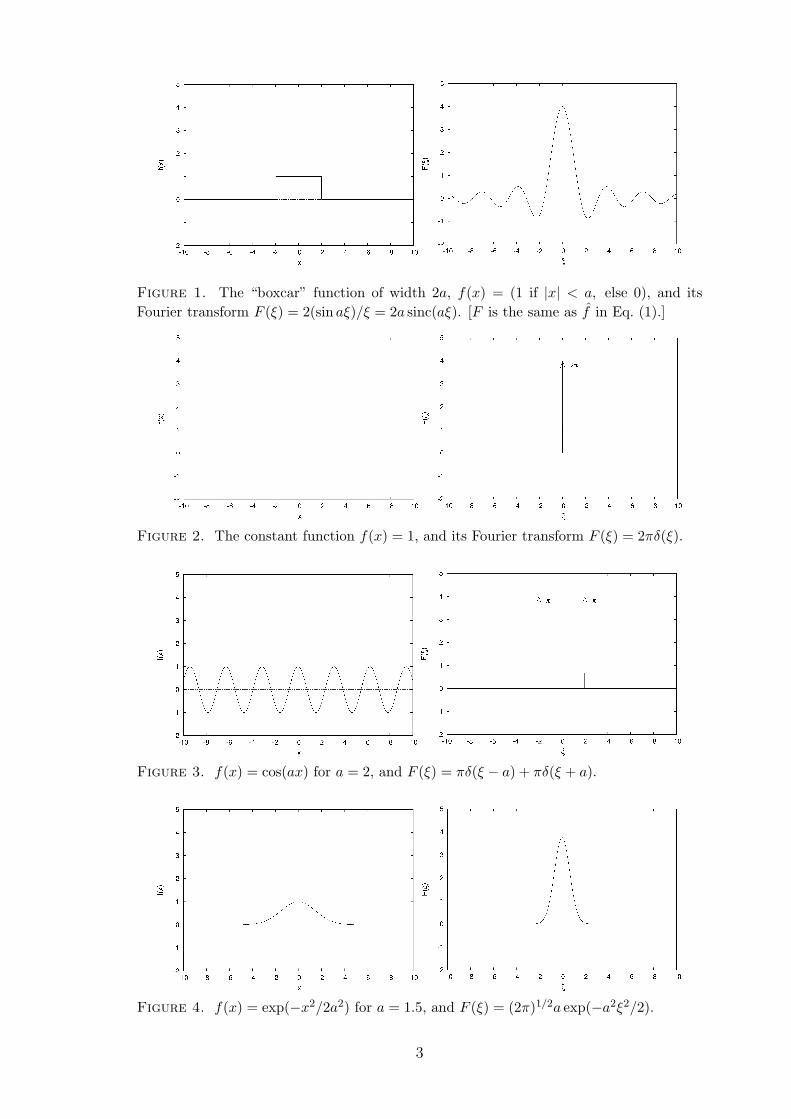
Figure 1. The “boxcar” function of width 2a, f(x) = (1 if |x| < a, else 0), and itsFourier transform F (ξ) = 2(sin aξ)/ξ = 2a sinc(aξ). [F is the same as f in Eq. (1).]

Figure 2. The constant function f(x) = 1, and its Fourier transform F (ξ) = 2πδ(ξ).

Figure 3. f(x) = cos(ax) for a = 2, and F (ξ) = πδ(ξ − a) + πδ(ξ + a).

Figure 4. f(x) = exp(−x2/2a2) for a = 1.5, and F (ξ) = (2π)1/2a exp(−a2ξ2/2).

3

2 The discrete Fourier transform

2.1 Definitions

Given N values u0, . . . , uN−1, the following holds:

uk =N−1∑j=0

uj e−i2πjk/N

uj =1

N

N−1∑k=0

uk ei2πjk/N

(7)

The first equation gives the discrete Fourier transform (DFT) of the sequence {uj};the second gives the inverse discrete Fourier transform of the sequence {uk}. uj areuk ar in general complex (cf. Sect. 1.3).

Note that although the formulae in Eq. (7) define the direct and inverse DTFs,they are almost never used to calculate them. The reason is that they are com-putationally inefficient for large N . (The number of arithmetic operations growsas N2.) Instead, an elegant algorithm called the Fast Fourier Transform (FFT) isused. This is really just a clever way of re-arranging the multiplications and sums in(7), using the properties of the exponential function, to reduce the total number ofarithmetic operations. (With the FFT, the number of operations grows as N lnN .)Mathematically, however, the result of the FFT is identical to Eq. (7).

As was the case for the continuous Fourier transform, the DFT comes in several dif-ferent variants depending on the placement of the normalization factor 1/N (whichcan be placed either in the direct or the inverse transform) and the sign of theimaginary unit in the exponentials. In other words, one has to look out for whichconventions are used in a particular application. In the project Signal analysis inastronomy the convention is that the factor 1/N is included in the direct transform.

Another complication is that vectors and matrices in some programming languages(including MATLAB) start at index 1 instead of 0 as in Eq. (7). For example, theMATLAB functions U = fft(u) and u = ifft(U) implement the formulae

U(k) =N∑j=1

u(j) e−i2π(j−1)(k−1)/N , k = 1 . . . N

u(j) =1

N

N∑k=1

U(k) ei2π(j−1)(k−1)/N , j = 1 . . . N

(8)

(using the FFT). These are equivalent to Eq. (7) using the substitution

u(j) = uj−1 (j = 1 . . . N), U(k) = uk−1 (k = 1 . . . N) (9)

2.2 Interpretation of the variables. Units

In physical applications, the values in the sequence u0, u1, . . . , uN−1 usually representsome measurable quantity (temperature, electrical voltage, intensity of light) in a

4

number of equidistant points along some spatial coordinate or time. There is thenalways a corresponding sequence of spatial or time coordinates

xj = xstart + j∆x, j = 0 . . . N − 1 (10)

such that uj is the value of the physical quantity at point xj. The sequence {uj}is a sampling of the physical quantity in N points with sampling interval ∆x. Thestarting point of the sampling, xstart, is often of little interest; however, it is alwaysimportant to know ∆x and N .

What is the interpretation of uk? These are complex values that specify the am-plitude (×N) and phase of the set of N Fourier components, that jointly exactlyrepresent the original sequence. The frequencies of the Fourier components form areequidistant,

fk = k∆f, k = 0 . . . N − 1 (11)

with ∆f = 1/(N∆x). The unit for f is the inverse of the unit for x. If x is in [m],then f is in [per m−1]; if x is in [s], then f is in [Hz]. Note that “ordinary” frequenciesare used here – no angular frequency or wave number – since the definition of theDFT uses 2πf in the exponentials.

When using MATLAB it is important to remember that the transformed value U(k)corresponds to frequency (k − 1)∆f , since the index of the array starts at 1.

2.3 Effects of the sampling

The DFT can be regarded as an approximation of the continuous FT, which itapproaches (after suitable normalization) when N goes to infinity and/or ∆x goesto zero. In practice, N and ∆x are always finite, which causes some undesirableeffects. Two important effects of the sampling are:

• Aliasing: Suppose that we sample the continuous function sin(2πfx) (of fre-quency f) in the points xj = j∆x, i.e., using the sampling frequency fs =1/∆x. It is then easy to see that the sampled points will be exactly the sameif we replace f by f +nfs in the sine function, where n is an integer. There isconsequently an infinitude of sine functions with different frequencies (aliases)that all look exactly the same after sampling. For a real function, there areeven more aliases, since the Fourier components at nfs + f and nfs − f arecomplex conjugate and therefore have the same amplitude. In particular, thecomponents at f and fs − f are complex conjugate. This becomes a prob-lem if the sampled signal contains real components with f > fs/2 ≡ fNy (theNyquist frequency), since they will then (falsely) appear also at fs − f < fNy.Therefore, if the continuous signal contains components up to fmax, it is nec-essary to choose ∆x < 1/(2fmax) in order to avoid aliasing. In other words,the minimum sampling frequency is 2fmax.

• Finite frequency resolution: The DFT of a sequence of length N∆x provides adecomposition into Fourier components that are separated by ∆f = 1/(N∆x).This means that if the signal contains components whose frequencies are sep-arated by less than ∆f , they cannot be distinguished in the DFT.

5

For example, if we know that a continuous signal contains two components withfrequencies fA and fB (where fA < fB), we can derive the minimum requirements interms of ∆x and N to enable unambiguous determination of the two components.First, the maximum sampling interval is given by twice the maximum frequencyin the signal, i.e., fs > 2fB or ∆x < 1/(2fB). Secondly, the minimum lengthof the sequence is given by the inverse of the required frequency resolution, orN∆x > 1/(fB − fA).

3 Convolution and filtering

3.1 Definition of convolution

The convolution3 of two continuous functions f(x) and g(x) is defined as

h(x) =∫ +∞

−∞f(x′)g(x− x′) dx′ (12)

which is often written symbolically

h = f ∗ g (13)

The convolution operator is commutative, g ∗ f = f ∗ g. A simple example willmake the meaning of Eq. (12) a little clearer. Suppose g(x) is the boxcar functionof width 2a and area 1, so that

g(x) =

1

2aif |x| < a

0 otherwise

(14)

Then

h(x) =∫ +∞

−∞f(x′)g(x− x′) dx′ = 1

2a

∫ x+a

x−af(x′) dx′ (15)

which is a so-called “running mean” of f(x) (that is, h(x) is the mean value of f(x′)for x′ ∈ [x−a, x+a]). For other functions g(x) one can regard the convolution f ∗ gas a “weighted running mean” of f(x).4 The convolution operator is graphicallyillustrated in Fig. 5.

Convolving the arbitrary function f(x) with Dirac’s delta leaves the function un-changed:

f(x) ∗ δ(x) = δ(x) ∗ f(x) =∫ +∞

−∞δ(x′)f(x− x′) dx′ =

∫ 0+

0−δ(x′)f(x− x′) dx′ = f(x)

(16)Convolution is in practice the same as filtering : the convolution suppresses or en-hances different Fourier components in the signal or image. A running mean sup-presses high frequencies and therefore acts as a low-pass filter (although there exist

3In Swedish: faltning, konvolvering or konvolution.4Strictly speaking one can only talk about the convolution as a running mean when g(x) has

unit area, as in the example above. Convolution is however defined for more general functions.

6

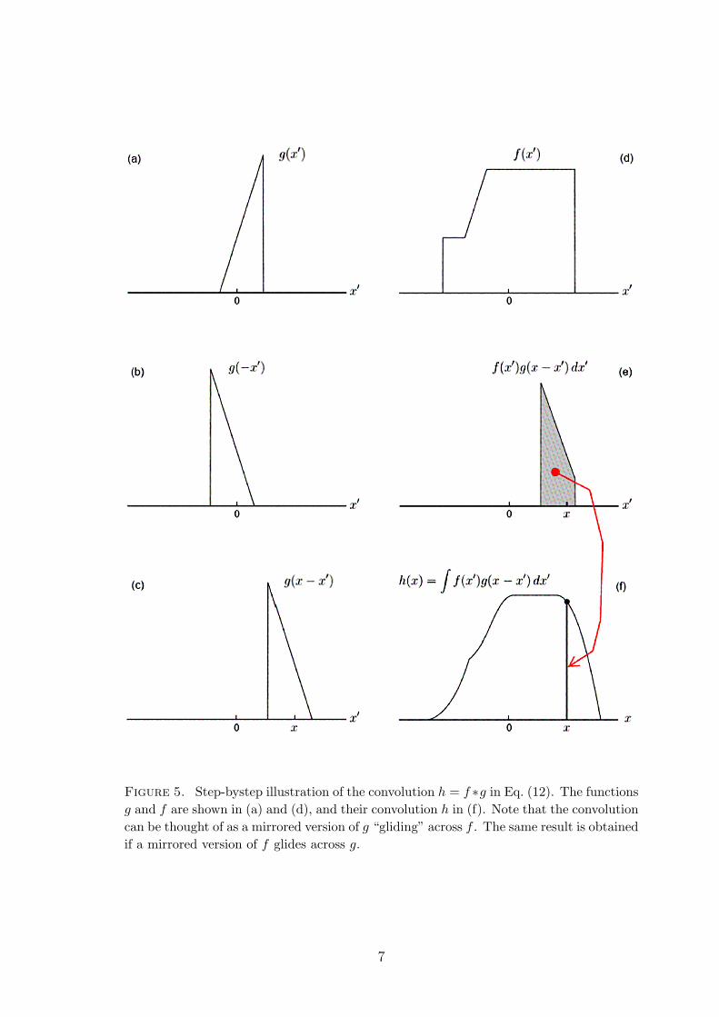
Figure 5. Step-bystep illustration of the convolution h = f ∗g in Eq. (12). The functionsg and f are shown in (a) and (d), and their convolution h in (f). Note that the convolutioncan be thought of as a mirrored version of g “gliding” across f . The same result is obtainedif a mirrored version of f glides across g.

7

more efficient filters for this). Convolution (or filtering) is useful for describing howa signal (f , for example an electric or acoustic signal, or an image) is affected by alinear system (e.g., electrical filter, resonance cavity, optics). The result (“outputsignal” h) is the convolution of the “input signal” f with the “impulse response”function g. The latter gets its name from the system’s response to a single short im-pulse (mathematically: f(x) = δ(x)), which according to Eq. (16) gives the outputsignal h = δ ∗ g = g.

For discrete functions (sequences or time series) {uj}, {vj} the convolution w = u∗vis defined in the corresponding manner by means of the sum

wj =∑k

ukvj−k (17)

In principle the sum extends over all k for which vj−k 6= 0. But since a finite sequencehas a limited range of index values, e.g. 0 . . . N−1, the sum is usually defined over thisrange. j − k should then be interpreted modulo N . This is equivalent to assumingthat the sequence is periodically extended to the left and right (with period N).

3.2 The convolution theorem

A central theorem in signal processing is the convolution theorem

h = f ∗ g ⇔ h = f .g (18)

which is valid for both continuous and discrete functions. Convolution in the spatialor time domain (x) is therefore equivalent to a multiplication in the correspondingfrequency domain (ξ). The converse is also true:

h = f.g ⇔ h = f ∗ g (19)

Using the convolution theorem, it is possible to compute the discrete convolutionw = u ∗ v much more efficiently (for large N) than by direct application of Eq. (17).Given the sequences {uj} and {vj} (both of length N) the recipe is:

1. Calculate the discrete Fourier transforms {uk} and {vk} using the FFT algo-rithm (note that {uk} and {vk} are complex, even if {uj} and {vj} are not)

2. Calculate wk = ukvk for k = 0 . . . N − 1

3. Calculate the inverse DFT of {wk}, which gives {wj} = {uj} ∗ {vj}.

It may seem surprising that Fourier transforming forth and back is more efficientthan a direct evaluation of the simple expression in Eq. (17). The reason is thatthe direct evaluation of Eq. (17) requires of the order of N2 multiplications andadditions, while each DFT in Step 1 and 3 above requires only of the order ofN lnN operations (using the FFT; see Sect. 2.1) and Step 2 only 6N operations.Thus, for sufficiently large N the above procedure will always be more efficient.

/LL 080822

8