Embed Size (px)
Citation preview
Wayne HuSTScI, May 2008
The Cosmology of
f (R)Models
for Cosmic Acceleration

Why Study f (R)?• Cosmic acceleration, like the cosmological constant, can either be
viewed as arising from
Missing, or dark energy, with w ≡ p/ρ < −1/3
Modification of gravity on large scales
Gµν = 8πG(TMµν + TDE
µν
)F (gµν) +Gµν = 8πGTM
µν
• Proof of principle models for both exist: quintessence, k-essence;DGP braneworld acceleration, f(R) modified action
• Compelling models for either explanation lacking
• Study models as illustrative toy models whose features can begeneralized

Parameterized Post-FriedmannDescription
• Smooth dark energy parameterized description on small scales:w(z) that completely defines expansion history, sound speeddefines structure formation
• Parameterized description of modified gravity acceleration
Many ad-hoc attempts violate energy-momentum conservation,Bianchi identities, gauge invariance; others incomplete
Parameterize the degrees of freedom in the effective dark energy
F (gµν) = 8πGTDEµν
retaining the metric structure of general relativity but withcomponent non-minimally dependent on metric, coupled to matter
Non-linear mechanism returns general relativity on small scales

Parameterized Post-FriedmannDescription
• Smooth dark energy parameterized description on small scales:w(z) that completely defines expansion history, sound speeddefines structure formation
• Parameterized description of modified gravity acceleration
• Many ad-hoc attempts violate energy-momentum conservation,Bianchi identities, gauge invariance; others incomplete
• Parameterize the degrees of freedom in the effective dark energy
F (gµν) = 8πGTDEµν
retaining the metric structure of general relativity but withcomponent non-minimally dependent on metric, coupled to matter
• Non-linear mechanism returns general relativity on small scales
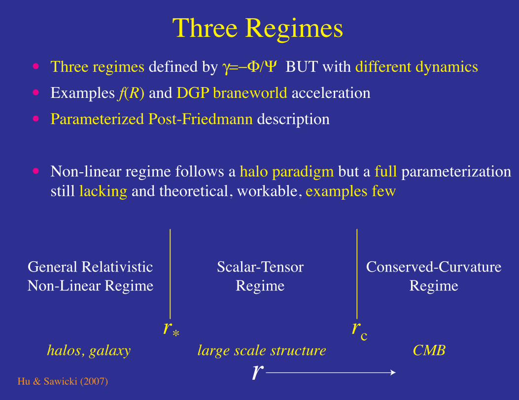
Three Regimes• Three regimes defined by γ=−Φ/Ψ BUT with different dynamics
• Examples f(R) and DGP braneworld acceleration
• Parameterized Post-Friedmann description
• Non-linear regime follows a halo paradigm but a full parameterization still lacking and theoretical, workable, examples few
Hu & Sawicki (2007)
r* rc
Scalar-TensorRegime
Conserved-CurvatureRegime
General RelativisticNon-Linear Regime
rhalos, galaxy large scale structure CMB

Outline• f(R) Basics and Background
• Linear Theory Predictions
• Nonlinear Regime
Solar System Tests
N-body Simulations
• Collaborators:
• Marcos Lima
• Hiro Oyaizu
• Hiranya Peiris
• Iggy Sawicki
• Yong-Seon Song see also Poster: Wenjuan Fang

Apologies to...[1] S. M. Carroll, V. Duvvuri, M. Trodden, and M. S. Turner, Phys. Rev. D70,
043528 (2004), astro-ph/0306438.[2] S. Nojiri and S. D. Odintsov, Int. J. Geom. Meth. Mod. Phys. 4, 115 (2007),
hep-th/0601213.[3] S. Capozziello, Int. J. Mod. Phys. D11, 483 (2002), gr-qc/0201033.[4] S. Capozziello, S. Carloni, and A. Troisi (2003), astro-ph/0303041.[5] S. Nojiri and S. D. Odintsov, Phys. Rev. D68, 123512 (2003), hep-
th/0307288.[6] S. Nojiri and S. D. Odintsov, Phys. Lett. B576, 5 (2003), hep-th/0307071.[7] V. Faraoni, Phys. Rev. D72, 124005 (2005), gr-qc/0511094.[8] A. de la Cruz-Dombriz and A. Dobado, Phys. Rev. D74, 087501 (2006), gr-
qc/0607118.[9] N. J. Poplawski, Phys. Rev. D74, 084032 (2006), gr-qc/0607124.
[10] A. W. Brookfield, C. van de Bruck, and L. M. H. Hall, Phys. Rev. D74,064028 (2006), hep-th/0608015.
[11] B. Li, K. C. Chan, and M. C. Chu (2006), astro-ph/0610794.[12] T. P. Sotiriou and S. Liberati, Annals Phys. 322, 935 (2007), gr-qc/0604006.[13] T. P. Sotiriou, Phys. Lett. B645, 389 (2007), gr-qc/0611107.[14] T. P. Sotiriou, Class. Quant. Grav. 23, 5117 (2006), gr-qc/0604028.[15] R. Bean, D. Bernat, L. Pogosian, A. Silvestri, and M. Trodden, Phys. Rev.
D75, 064020 (2007), astro-ph/0611321.[16] S. Baghram, M. Farhang, and S. Rahvar, Phys. Rev. D75, 044024 (2007),
astro-ph/0701013.[17] D. Bazeia, B. Carneiro da Cunha, R. Menezes, and A. Y. Petrov (2007),
hep-th/0701106.[18] B. Li and J. D. Barrow, Phys. Rev. D75, 084010 (2007), gr-qc/0701111.[19] S. Bludman (2007), astro-ph/0702085.[20] T. Rador (2007), hep-th/0702081.[21] T. Rador, Phys. Rev. D75, 064033 (2007), hep-th/0701267.[22] L. M. Sokolowski (2007), gr-qc/0702097.[23] V. Faraoni, Phys. Rev. D75, 067302 (2007), gr-qc/0703044.[24] V. Faraoni, Phys. Rev. D74, 104017 (2006), astro-ph/0610734.[25] S. Nojiri and S. D. Odintsov, Gen. Rel. Grav. 36, 1765 (2004), hep-
th/0308176.[26] P. Wang and X.-H. Meng, TSPU Vestnik 44N7, 40 (2004), astro-ph/0406455.[27] X.-H. Meng and P. Wang, Gen. Rel. Grav. 36, 1947 (2004), gr-qc/0311019.[28] M. C. B. Abdalla, S. Nojiri, and S. D. Odintsov, Class. Quant. Grav. 22,
L35 (2005), hep-th/0409177.[29] G. Cognola, E. Elizalde, S. Nojiri, S. D. Odintsov, and S. Zerbini, JCAP
0502, 010 (2005), hep-th/0501096.[30] S. Capozziello, V. F. Cardone, and A. Troisi, Phys. Rev. D71, 043503 (2005),
astro-ph/0501426.[31] G. Allemandi, A. Borowiec, M. Francaviglia, and S. D. Odintsov, Phys. Rev.
D72, 063505 (2005), gr-qc/0504057.[32] T. Koivisto and H. Kurki-Suonio, Class. Quant. Grav. 23, 2355 (2006), astro-
ph/0509422.[33] T. Clifton and J. D. Barrow, Phys. Rev. D72, 103005 (2005), gr-qc/0509059.[34] O. Mena, J. Santiago, and J. Weller, Phys. Rev. Lett. 96, 041103 (2006),
astro-ph/0510453.[35] M. Amarzguioui, O. Elgaroy, D. F. Mota, and T. Multamaki, Astron. Astro-
phys. 454, 707 (2006), astro-ph/0510519.[36] I. Brevik, Int. J. Mod. Phys. D15, 767 (2006), gr-qc/0601100.[37] T. Koivisto, Phys. Rev. D73, 083517 (2006), astro-ph/0602031.[38] S. E. Perez Bergliaffa, Phys. Lett. B642, 311 (2006), gr-qc/0608072.[39] G. Cognola, M. Gastaldi, and S. Zerbini (2007), gr-qc/0701138.[40] S. Capozziello and R. Garattini, Class. Quant. Grav. 24, 1627 (2007), gr-
qc/0702075.[41] S. Nojiri and S. D. Odintsov, Phys. Rev. D74, 086005 (2006), hep-
th/0608008.[42] S. Nojiri and S. D. Odintsov (2006), hep-th/0610164.[43] S. Capozziello, S. Nojiri, S. D. Odintsov, and A. Troisi, Phys. Lett. B639,
135 (2006), astro-ph/0604431.[44] S. Fay, S. Nesseris, and L. Perivolaropoulos (2007), gr-qc/0703006.[45] S. Fay, R. Tavakol, and S. Tsujikawa, Phys. Rev. D75, 063509 (2007), astro-
ph/0701479.[46] S. Nojiri, S. D. Odintsov, and M. Sasaki, Phys. Rev. D71, 123509 (2005),
hep-th/0504052.[47] M. Sami, A. Toporensky, P. V. Tretjakov, and S. Tsujikawa, Phys. Lett.
B619, 193 (2005), hep-th/0504154.[48] G. Calcagni, S. Tsujikawa, and M. Sami, Class. Quant. Grav. 22, 3977
(2005), hep-th/0505193.[49] S. Tsujikawa and M. Sami, JCAP 0701, 006 (2007), hep-th/0608178.[50] Z.-K. Guo, N. Ohta, and S. Tsujikawa, Phys. Rev. D75, 023520 (2007), hep-
th/0610336.[51] A. K. Sanyal, Phys. Lett. B645, 1 (2007), astro-ph/0608104.[52] B. M. Leith and I. P. Neupane (2007), hep-th/0702002.[53] B. M. N. Carter and I. P. Neupane, JCAP 0606, 004 (2006), hep-th/0512262.[54] T. Koivisto and D. F. Mota, Phys. Rev. D75, 023518 (2007), hep-th/0609155.[55] T. Koivisto and D. F. Mota, Phys. Lett. B644, 104 (2007), astro-ph/0606078.[56] S. Nojiri, S. D. Odintsov, and M. Sami, Phys. Rev. D74, 046004 (2006),
hep-th/0605039.[57] S. Nojiri and S. D. Odintsov (2006), hep-th/0611071.[58] G. Cognola, E. Elizalde, S. Nojiri, S. Odintsov, and S. Zerbini, Phys. Rev.
D75, 086002 (2007), hep-th/0611198.[59] S. Nojiri and S. D. Odintsov, Phys. Lett. B631, 1 (2005), hep-th/0508049.[60] G. Cognola, E. Elizalde, S. Nojiri, S. D. Odintsov, and S. Zerbini, Phys. Rev.
D73, 084007 (2006), hep-th/0601008.[61] Y.-S. Song, W. Hu, and I. Sawicki, Phys. Rev. D75, 044004 (2007), astro-
ph/0610532.[62] S. Nojiri, S. D. Odintsov, and P. V. Tretyakov (2007), arXiv:0704.2520 [hep-
th].[63] T. Multamaki and I. Vilja, Phys. Rev. D73, 024018 (2006), astro-
ph/0506692.[64] R. P. Woodard (2006), astro-ph/0601672.[65] T. P. Sotiriou, Gen. Rel. Grav. 38, 1407 (2006), gr-qc/0507027.[66] J. A. R. Cembranos, Phys. Rev. D73, 064029 (2006), gr-qc/0507039.[67] G. Allemandi, M. Francaviglia, M. L. Ruggiero, and A. Tartaglia, Gen. Rel.
Grav. 37, 1891 (2005), gr-qc/0506123.[68] M. L. Ruggiero and L. Iorio, JCAP 0701, 010 (2007), gr-qc/0607093.[69] T. P. Sotiriou and E. Barausse, Phys. Rev. D75, 084007 (2007), gr-
qc/0612065.[70] C.-G. Shao, R.-G. Cai, B. Wang, and R.-K. Su, Phys. Lett. B633, 164 (2006),
gr-qc/0511034.[71] A. J. Bustelo and D. E. Barraco, Class. Quant. Grav. 24, 2333 (2007), gr-
qc/0611149.[72] G. J. Olmo, Phys. Rev. D75, 023511 (2007), gr-qc/0612047.
[73] P.-J. Zhang (2007), astro-ph/0701662.[74] K. Kainulainen, J. Piilonen, V. Reijonen, and D. Sunhede (2007),
arXiv:0704.2729 [gr-qc].[75] T. Chiba, Phys. Lett. B575, 1 (2003), astro-ph/0307338.[76] A. L. Erickcek, T. L. Smith, and M. Kamionkowski, Phys. Rev. D74, 121501
(2006), astro-ph/0610483.[77] T. Chiba, T. L. Smith, and A. L. Erickcek (2006), astro-ph/0611867.[78] J. Khoury and A. Weltman, Phys. Rev. D69, 044026 (2004), astro-
ph/0309411.[79] I. Navarro and K. Van Acoleyen (2006), gr-qc/0611127.[80] T. Faulkner, M. Tegmark, E. F. Bunn, and Y. Mao (2006), astro-ph/0612569.[81] D. F. Mota and J. D. Barrow, Phys. Lett. B581, 141 (2004), astro-
ph/0306047.[82] D. F. Mota and J. D. Barrow, Mon. Not. Roy. Astron. Soc. 349, 291 (2004),
astro-ph/0309273.[83] L. Amendola, D. Polarski, and S. Tsujikawa (2006), astro-ph/0603703.[84] I. Sawicki and W. Hu, Phys. Rev. D75, 127502 (2007), astro-ph/0702278.[85] P. Zhang, Phys. Rev. D73, 123504 (2006), astro-ph/0511218.[86] A. A. Starobinsky, Phys. Lett. B91, 99 (1980).[87] T. Faulkner, M. Tegmark, E. F. Bunn, and Y. Mao (2006), astro-ph/0612569.[88] A. Vikman, Phys. Rev. D71, 023515 (2005), astro-ph/0407107.[89] W. Hu, Phys. Rev. D 71, 047301 (2005), astro-ph/0410680.[90] Z.-K. Guo, Y.-S. Piao, X.-M. Zhang, and Y.-Z. Zhang, Phys. Lett. B608,
177 (2005), astro-ph/0410654.[91] L. Amendola and S. Tsujikawa (2007), arXiv:0705.0396 [astro-ph].[92] A. D. Dolgov and M. Kawasaki, Phys. Lett. B573, 1 (2003), astro-
ph/0307285.[93] M. D. Seifert (2007), gr-qc/0703060.[94] J. A. R. Cembranos, Phys. Rev. D73, 064029 (2006), gr-qc/0507039.[95] J. N. Bahcall, A. M. Serenelli, and S. Basu, Astrophys. J. Lett. 621, L85
(2005), arXiv:astro-ph/0412440.[96] J. E. Vernazza, E. H. Avrett, and R. Loeser, Astrophys. J. Supp. 45, 635
(1981).[97] E. C. Sittler, Jr. and M. Guhathakurta, Astrophys. J. 523, 812 (1999).[98] C. M. Will, Living Reviews in Relativity 9 (2006), URL http://www.
livingreviews.org/lrr-2006-3.[99] A. Klypin, H. Zhao, and R. S. Somerville, Astrophys. J. 573, 597 (2002),
astro-ph/0110390.
f (R) Basics

Cast of f (R) Characters• R: Ricci scalar or “curvature”
• f(R): modified action (Starobinsky 1980; Carroll et al 2004)
S =
∫d4x
√−g[R + f(R)
16πG+ Lm
]

Cast of f (R) Characters• R: Ricci scalar or “curvature”
• f(R): modified action (Starobinsky 1980; Carroll et al 2004)
S =
∫d4x
√−g[R + f(R)
16πG+ Lm
]• fR ≡ df/dR: additional propagating scalar degree of freedom
(metric variation)
• fRR ≡ d2f/dR2: Compton wavelength of fR squared, inversemass squared
• B: Compton wavelength of fR squared in units of the Hubblelength
B ≡ fRR
1 + fR
R′ H
H ′
• ′ ≡ d/d ln a: scale factor as time coordinate

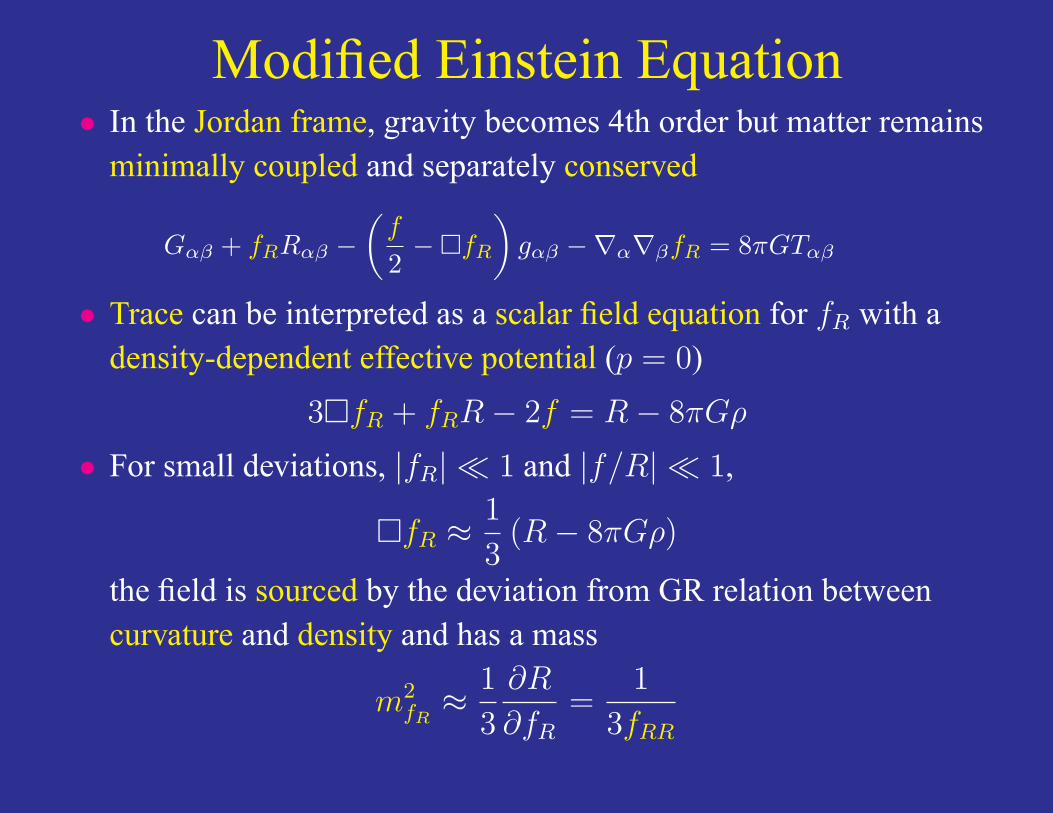
ModifiedEinstein Equation• In theJordan frame, gravity becomes 4th order but matter remains
minimally coupledand separatelyconserved
Gαβ + fRRαβ −(
f
2−fR
)gαβ −∇α∇βfR = 8πGTαβ
• Tracecan be interpreted as ascalar field equationfor fR with adensity-dependent effective potential(p = 0)
3fR + fRR− 2f = R− 8πGρ
Modified Einstein Equation• In the Jordan frame, gravity becomes 4th order but matter remains
minimally coupled and separately conserved
Gαβ + fRRαβ −(
f
2−fR
)gαβ −∇α∇βfR = 8πGTαβ
• Trace can be interpreted as a scalar field equation for fR with adensity-dependent effective potential (p = 0)
3fR + fRR− 2f = R− 8πGρ
• For small deviations, |fR| 1 and |f/R| 1,
fR ≈1
3(R− 8πGρ)
the field is sourced by the deviation from GR relation betweencurvature and density and has a mass
m2fR≈ 1
3
∂R
∂fR
=1
3fRR

Effective Potential• Scalar fR rolls in an effective potential that depends on density• At high density, extrema is at GR R=8πGρ• Minimum for B>0, pinning field to |fR| <<1 , maximum for B<0
Sawicki & Hu (2007)
-1
0
1
10-5 1
0
2
4
|fR|
effe
ctiv
e po
tent
ial
B<0
B>0increasing ρ
increasingρ

f (R) Expansion History
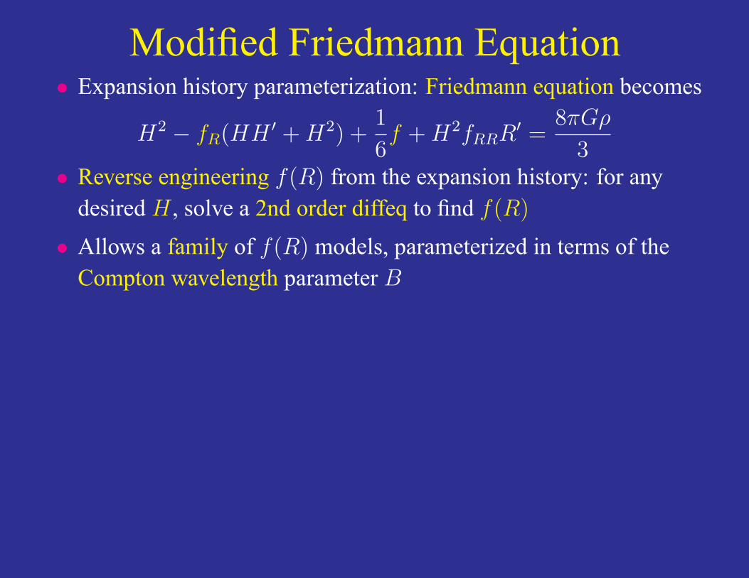
Modified Friedmann Equation• Expansion history parameterization: Friedmann equation becomes
H2 − fR(HH ′ +H2) +1
6f +H2fRRR
′ =8πGρ
3• Reverse engineering f(R) from the expansion history: for any
desired H , solve a 2nd order diffeq to find f(R)
• Allows a family of f(R) models, parameterized in terms of theCompton wavelength parameter B
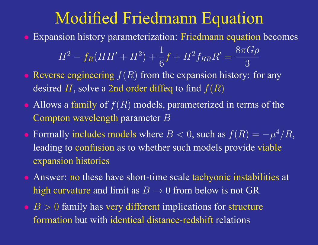
• Formally includes models where B < 0, such as f(R) = −µ4/R,leading to confusion as to whether such models provide viableexpansion histories
• Answer: no these have short-time scale tachyonic instabilities athigh curvature and limit as B → 0 from below is not GR
• B > 0 family has very different implications for structureformation but with identical distance-redshift relations

Hu, Huterer & Smith (2006)
Expansion History Family of f(R)• Each expansion history, matched by dark energy model [w(z),ΩDE,H0] corresponds to a family of f(R) models due to its 4th order nature• Parameterized by B ∝ fRR = d2f/dR2 evaluated at z=0
Song, Hu & Sawicki (2006)
10
-0.6
-0.4
-0.2
0
100 1000R/H0
2
f (R)
/R

Hu, Huterer & Smith (2006)
Expansion History Family of f(R)• Each expansion history, matched by dark energy model [w(z),ΩDE,H0] corresponds to a family of f(R) models due to its 4th order nature• Parameterized by B ∝ fRR = d2f/dR2 evaluated at z=0
Song, Hu & Sawicki (2006)
10
-0.6
-0.4
-0.2
0
100 1000R/H0
2
f (R)
/RB0=
0-0.3
-1 -3

Hu, Huterer & Smith (2006)
Expansion History Family of f(R)• Each expansion history, matched by dark energy model [w(z),ΩDE,H0] corresponds to a family of f(R) models due to its 4th order nature• Parameterized by B ∝ fRR = d2f/dR2 evaluated at z=0
Song, Hu & Sawicki (2006)
10
-0.6
-0.4
-0.2
0
100 1000R/H0
2
f (R)
/RB0=
3
10.3
0-0.3
-1 -3
Hu, Huterer & Smith (2006)
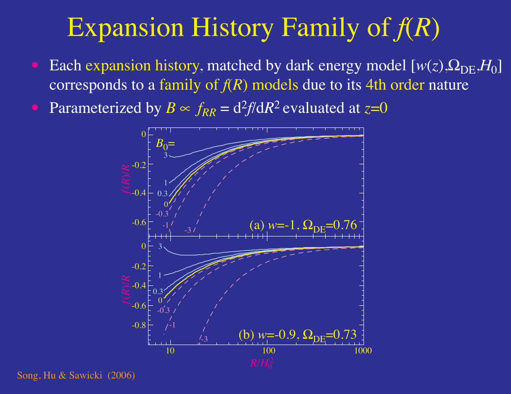
Expansion History Family of f(R)• Each expansion history, matched by dark energy model [w(z),ΩDE,H0] corresponds to a family of f(R) models due to its 4th order nature• Parameterized by B ∝ fRR = d2f/dR2 evaluated at z=0
Song, Hu & Sawicki (2006)
10
-0.8
-0.6
-0.6
-0.4
-0.2
0
-0.4
-0.2
0
100 1000R/H0
2
f (R)
/Rf (
R)/R
B0=3
3
1
1
0.3
0.3
0
0
-0.3
-0.3
-1
-1
-3
-3
(a) w=-1, ΩDE=0.76
(b) w=-0.9, ΩDE=0.73

Instability at High Curvature• Tachyonic instability for negative mass squared B<0 makes high curvature regime increasingly unstable: high density ≠ high curvature• Linear metric perturbations immediately drop the expansion history to low curvature solution
Sawicki & Hu (2007)
curv
atur
e R
110-510-10
1
1010
1020
1030
a
ΛCDM
Β>0
Β<0
f (R) Linear Theory

Curvature Conservation• On superhorizon scales, energy momentum conservation and
expansion history constrain the evolution of metric fluctuations(Bertschinger 2006)
• For adiabatic perturbations in a flat universe, conservation ofcomoving curvature applies ζ ′ = 0 where ′ ≡ d/d ln a (Bardeen 1980)
• Gauge transformation to Newtonian gauge
ds2 = −(1 + 2Ψ)dt2 + a2(1 + 2Φ)dx2
yields (Hu & Eisenstein 1999)
Φ′′ −Ψ′ − H ′′
H ′ Φ′ −(H ′
H− H ′′
H ′
)Ψ = 0
• Modified gravity theory supplies the closure relationshipΦ = −γ(ln a)Ψ between and expansion history H = a/a suppliesrest.

Linear Theory for f (R)• In f(R) model, “superhorizon” behavior persists until Compton
wavelength smaller than fluctuation wavelength B1/2(k/aH) < 1
• Once Compton wavelength becomes larger than fluctuation
B1/2(k/aH) > 1
perturbations are in scalar-tensor regime described by γ = 1/2.

Linear Theory for f (R)• In f(R) model, “superhorizon” behavior persists until Compton
wavelength smaller than fluctuation wavelength B1/2(k/aH) < 1
• Once Compton wavelength becomes larger than fluctuation
B1/2(k/aH) > 1
perturbations are in scalar-tensor regime described by γ = 1/2.
• Small scale density growth enhanced and
8πGρ > R
low curvature regime with order unity deviations from GR
• Transitions in the non-linear regime where the Comptonwavelength can shrink via chameleon mechanism
• Given kNL/aH 1, even very small fR have scalar-tensor regime

Deviation Parameter• Express the 4th order nature of equations as a deviation parameter
Φ′′ −Ψ′ − H ′′
H ′ Φ′ −(H ′
H− H ′′
H ′
)Ψ =
(k
aH
)2
Bε
• Einstein equation become a second order equation for ε
f(R) = −M2+2n/Rn

Deviation Parameter• Express the 4th order nature of equations as a deviation parameter
Φ′′ −Ψ′ − H ′′
H ′ Φ′ −(H ′
H− H ′′
H ′
)Ψ =
(k
aH
)2
Bε
• Einstein equation become a second order equation for ε
• In high redshift, high curvature R limit this is
ε′′ +
(7
2+ 4
B′
B
)ε′ +
2
Bε =
1
B× metric sources
B =fRR
1 + fR
R′ H
H ′
• R→∞, B → 0 and for B < 0 short time-scale tachyonicinstability appears making previous models not cosmologicallyviable
f(R) = −M2+2n/Rn

Hu, Huterer & Smith (2006)
Potential Growth• On the stable B>0 branch, potential evolution reverses from decay to growth as wavelength becomes smaller than Compton scale• Quasistatic equilibrium reached in linear theory with γ=−Φ/Ψ=1/2 until non-linear effects restore γ=1
Song, Hu & Sawicki (2006)
0.1 10.01a
Φ- /
Φi
weff=-1, ΩDE=0.76, B0=1 ΛCDM
10
1
00.8
0.9
1
1.2(Φ−Ψ)/2 k/aH0 =100

PPF Correspondence• On large scales, Bianchi identity requires covariant conservation of
effective dark energy leaving:
Metric ratio of Newtonian gravitational potentialsg(a, k) = (Φ + Ψ)/(Φ−Ψ)
First relationship with the matter fluctuations fζ(a)
• On linear scales, time-derivatives of metric can be dropped leadingto a Poisson-like equation with:
Metric ratio g(a, k) = (Φ + Ψ)/(Φ−Ψ)
Second relationship with the matter fluctuations fG(a)
• On non-linear scales associated with collapsed objects, acceptablemodifications must return general relativity
Transition between linear “2 halo” and non-linear “1 halo” regime

Hu, Huterer & Smith (2006)
PPF Description• Metric and matter evolution well-matched by PPF description• Standard GR tools apply (CAMB), self-consistent, gauge invar. [see Wenjuan Fang poster: Fang et al (2008)]
Hu & Sawicki (2007); Hu (2008)
0.1 1a
1.1
1.0
0.9
0.8
Φ−
/Φi
f(R)PPF
k/H0=0.1
30
100
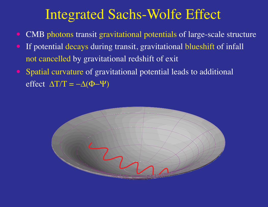
Integrated Sachs-Wolfe Effect• CMB photons transit gravitational potentials of large-scale structure• If potential decays during transit, gravitational blueshift of infall not cancelled by gravitational redshift of exit• Spatial curvature of gravitational potential leads to additional effect ∆T/T = −∆(Φ−Ψ)

Integrated Sachs-Wolfe Effect• CMB photons transit gravitational potentials of large-scale structure• If potential decays during transit, gravitational blueshift of infall not cancelled by gravitational redshift of exit• Spatial curvature of gravitational potential leads to additional effect ∆T/T = −∆(Φ−Ψ)

Hu, Huterer & Smith (2006)
ISW Quadrupole• Reduction of potential decay can eliminate the ISW effect at the quadrupole for B0~3/2• In conjunction with a change in the initial power spectrum can also bring the total quadrupole closer in ensemble average to the observed quadrupole
Song, Hu & Sawicki (2006)
1
103
102
2 3 4 5B0
6C2/2
π (µ
Κ2 )
ISW quadrupole
total quadrupoleΛCDM

ISW Quadrupole• Reduction of large angle anisotropy for B0~1 for same expansion history and distances as ΛCDM• Well-tested small scale anisotropy unchanged
10
3000
1000
100 1000multipole l
l(l+1
)Cl
/2π
(µK
2 )
B00 (ΛCDM)
1/23/2
TT
Song, Hu & Sawicki (2006)
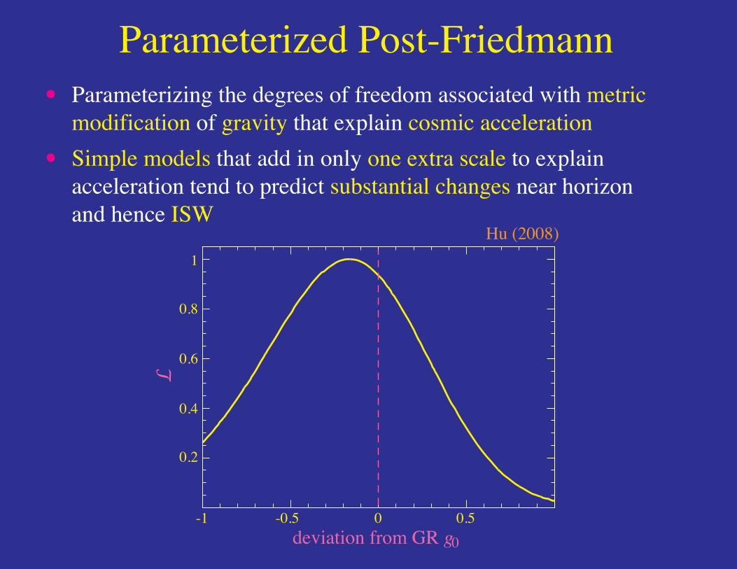
Parameterized Post-Friedmann• Parameterizing the degrees of freedom associated with metric modification of gravity that explain cosmic acceleration• Simple models that add in only one extra scale to explain acceleration tend to predict substantial changes near horizon and hence ISW
-1 -0.5
0.2
0.4
0.6
0.8
1
0 0.5deviation from GR g0
Hu (2008)

ISW-Galaxy Correlation• Decaying potential: galaxy positions correlated with CMB
• Growing potential: galaxy positions anticorrelated with CMB
• Observations indicate correlation
Hu, Huterer & Smith (2006)
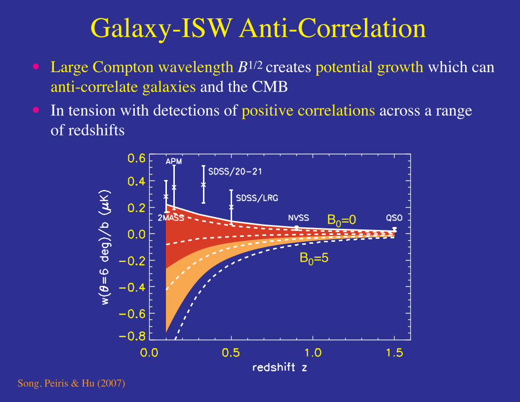
Galaxy-ISW Anti-Correlation• Large Compton wavelength B1/2 creates potential growth which can anti-correlate galaxies and the CMB• In tension with detections of positive correlations across a range of redshifts
Song, Peiris & Hu (2007)
B0=5
B0=0

Linear Power Spectrum• Linear real space power spectrum enhanced on small scales• Degeneracy with galaxy bias and lack of non-linear predictions leave constraints from shape of power spectrum
0.001 0.01 0.1
k (h/Mpc)
P L(k
) (M
pc/h
)3
104
103
B01
0.10.01
0.0010 (ΛCDM)

Hu, Huterer & Smith (2006)
Power Spectrum Data• Linear power spectrum enhancement fits SDSS LRG data better than ΛCDM but• Shape expected to be altered by non-linearities
Song, Peiris & Hu (2007)
0.10.01
3
10
30
k (h/Mpc)
P(k)
(10
4 Mpc
3 /h3 )
ΛCDM(non-linear fit)
f(r)
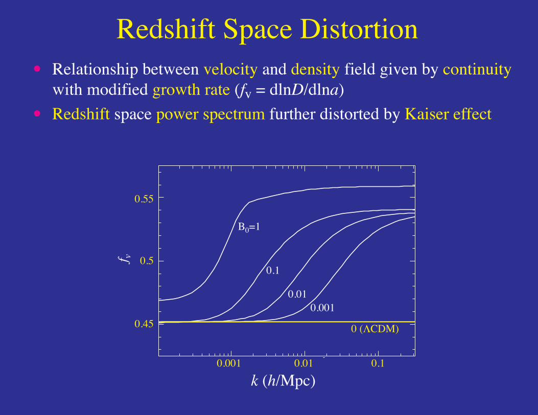
Redshift Space Distortion• Relationship between velocity and density field given by continuity with modified growth rate (fv = dlnD/dlna)• Redshift space power spectrum further distorted by Kaiser effect
0.001
0.45
0.5
0.55
0.01 0.1
k (h/Mpc)
f v
B0=1
0.1
0.010.001
0 (ΛCDM)

Viable f (R) Models

Engineering f (R) Models• Mimic ΛCDM at high redshift
• Accelerate the expansion at low redshift without a cosmologicalconstant
• Sufficient freedom to vary expansion history withinobservationally allowed range
• Contain the phenomenology of ΛCDM in both cosmology andsolar system tests as a limiting case for the purposes ofconstraining small deviations
• Suggests
f(R) ∝ Rn
Rn + const.
such that modifications vanish as R→ 0 and go to a constant asR→∞
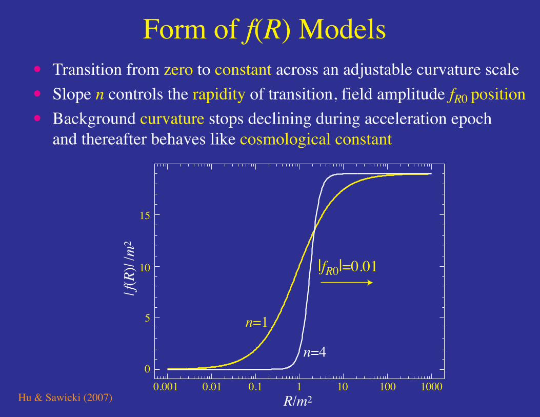
Form of f(R) Models • Transition from zero to constant across an adjustable curvature scale• Slope n controls the rapidity of transition, field amplitude fR0 position• Background curvature stops declining during acceleration epoch and thereafter behaves like cosmological constant
Hu & Sawicki (2007) R/m2
| f(R
)| /m
2
10.10.010.001 10 100 10000
5
10
15
n=1
n=4
|fR0|=0.01

Expansion History• Effective equation of state weff scales with field amplitude fR0
• Crosses the phantom divide at a redshift that decreases with n
• Signature of degrees of freedom in dark energy beyond standard kinetic and potential energy of k-essence or quintessence or modified gravity
Hu & Sawicki (2007)
0.01
0.01
0.03
0.03
0.1= | fR0|
0.1=| fR0|
z
wef
fw
eff
2
-0.95
-0.9
-1
-1.1
-1
-1.05
4 6 8
(b) n=4
(a) n=1

f (R) Solar System Tests

Solar Profile• Density profile of Sun is not a constant density sphere - interior photosphere, chromosphere, corona• Density drops by ~25 orders of magnitude - does curvature follow?
Hu & Sawicki (2007) r/r
ρ (g
cm
-3)
0.1 1 10 100 1000
10-20
10-10
1
R/8πG (n=4, | fR0|=0.1)ρ

f (R) Chameleon• Scalar f(R) takes on a chameleon form – mass increases with
density at minimum of effective potential (Khoury & Weltman 2004)
∇2fR ≈1
3(R− 8πGρ)
• Solutions either high curvature R ≈ 8πGρ and small fieldgradient, or low curvature R 8πGρ and large field gradient∇2fR ≈ −8πGρ/3 depending on Compton scale vs size of object
• Low curvature solution places a maximum for change in the fieldthat is related to the gravitational potential Φ
∆fR ≤2
3Φ ,
• If required |∆fR| Φ the interior must be at high curvature tosuppress the changes and hence the source R− 8πGρ ≈ 0 comesonly from a thin shell of mass
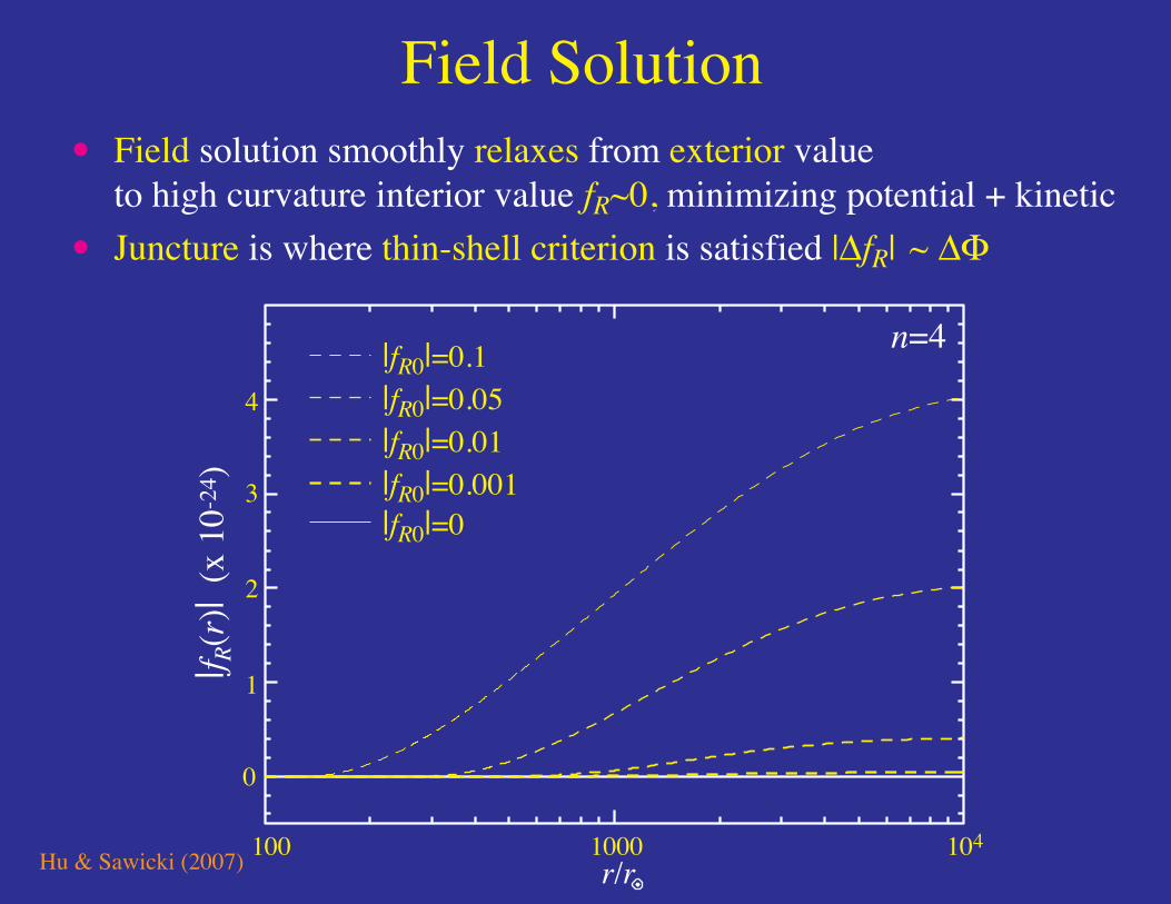
Field Solution• Field solution smoothly relaxes from exterior value to high curvature interior value fR~0, minimizing potential + kinetic• Juncture is where thin-shell criterion is satisfied |∆fR| ~ ∆Φ
Hu & Sawicki (2007) r/r100 1000 104
|f R(r
)| (x
10-
24)
0
1
2
3
4|fR0|=0.1|fR0|=0.05|fR0|=0.01|fR0|=0.001|fR0|=0
n=4

Solar Curvature• Curvature drops suddenly as field moves slightly from zero• Enters into low curvature regime where R<8πGρ
Hu & Sawicki (2007) r/r100 1000 104
R/8π
G (g
cm
-3)
10-24
10-23
|fR0|=0.001|fR0|=0.01|fR0|=0.05|fR0|=0.1
ρ
n=4
f (R) Chameleon• The field fR does not then sit at the potential minimum everywhere
but instead minimizes the cost of potential and kinetic gradientenergy
• A solution for fR is a solution for R and the metric is fixed to beconsistent with the curvature
|γ − 1| ≈ |∆fR(r)|Φ(r)
• Constraints on |γ − 1| place constraints on the change in the fieldamplitude from the interior of the sun to the exterior of the solarsystem
• A second transition occurs from the field changes from in thegalaxy to cosmology
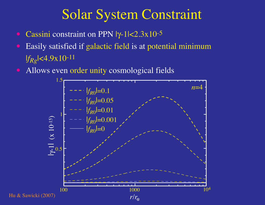
Solar System Constraint• Cassini constraint on PPN |γ-1|<2.3x10⁻⁵
• Easily satisfied if galactic field is at potential minimum |fRg|<4.9x10⁻¹¹
• Allows even order unity cosmological fields
Hu & Sawicki (2007) r/r100 1000
|γ-1|
(x 1
0-15
)
0.5
1
1.5
104
n=4|fR0|=0.1|fR0|=0.05|fR0|=0.01|fR0|=0.001|fR0|=0

Galactic Thin Shell• Galaxy must have a thin shell for interior to remain at high curvature• Rotation curve v/c~10-3, Φ~10-6~|∆fR| limits cosmological field • Has the low cosmological curvature propagated through local group and galactic exterior?
Hu & Sawicki (2007) r (kpc)100 1000
R/8π
G (g
cm
-3)
10-28
10-27
10-26
10-25
10-24
|fR0|=0.5 x10⁻⁶
|fR0|=1.0 x10⁻⁶
|fR0|=2.0 x10⁻⁶
ρ
n=1/2

f (R) Non-Linear Evolution
PPF Correspondence• Onlarge scales, Bianchi identity requires covariant conservation of
effective dark energy leaving:
Metric ratio of Newtonian gravitational potentialsg(a, k) = (Φ + Ψ)/(Φ−Ψ)
First relationship with the matter fluctuations fζ(a)
• On linear scales, time-derivatives of metric can be dropped leadingto a Poisson-like equation with:
Metric ratio g(a, k) = (Φ + Ψ)/(Φ−Ψ)
Second relationship with the matter fluctuations fG(a)
• On non-linear scales associated with collapsed objects, acceptablemodifications must return general relativity
Transition between linear “2 halo” and non-linear “1 halo” regime

Hu, Huterer & Smith (2006)
PPF Halo Model• Two halo term behaves as in linear PPF description• One halo term interpolates back to GR with same expansion history
Hu & Sawicki (2007)
f(R)
0.10.01 1 10k (h/Mpc)
P(k)
/PG
R(k
)-1
0.2
0.4
0.6
0.8
cnl=0
1
0.01
0.1

N-body• For f(R) the field equation
∇2fR ≈1
3(δR(fR)− 8πGδρ)
is the non-linear equation that returns general relativity.
• Supplement that with the modified Poisson equation
∇2Ψ =16πG
3δρ− 1
6δR(fR)
and the usual motion of matter in a gravitational potential Ψ
• Prescription for N -body code
• PM for the Poisson equation, relaxation method for fR
• Initial conditions set to GR at high redshift
Hu, Huterer & Smith (2006)
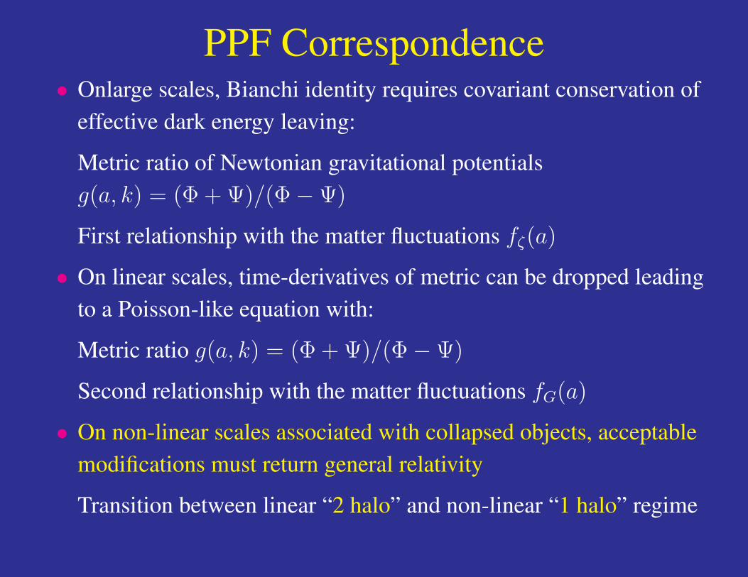
N-body Power Spectrum• 5123 PM-relaxation code resolves the chameleon transition to GR
Oyaizu et al. (2008) k (h/Mpc)
P(k)
/PG
R(k
)-1
0.1 1
0
1
0.5
linear

Hu, Huterer & Smith (2006)
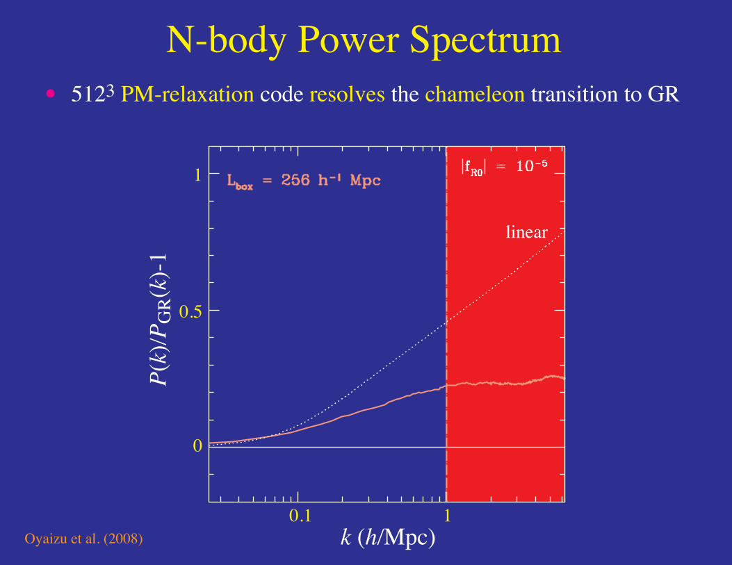
N-body Power Spectrum• 5123 PM-relaxation code resolves the chameleon transition to GR
Oyaizu et al. (2008) k (h/Mpc)
P(k)
/PG
R(k
)-1
0.1 1
0
1
0.5
linear
Hu, Huterer & Smith (2006)
N-body Power Spectrum• 5123 PM-relaxation code resolves the chameleon transition to GR
Oyaizu et al. (2008) k (h/Mpc)
P(k)
/PG
R(k
)-1
0.1 1
0
1
0.5
linear
Hu, Huterer & Smith (2006)
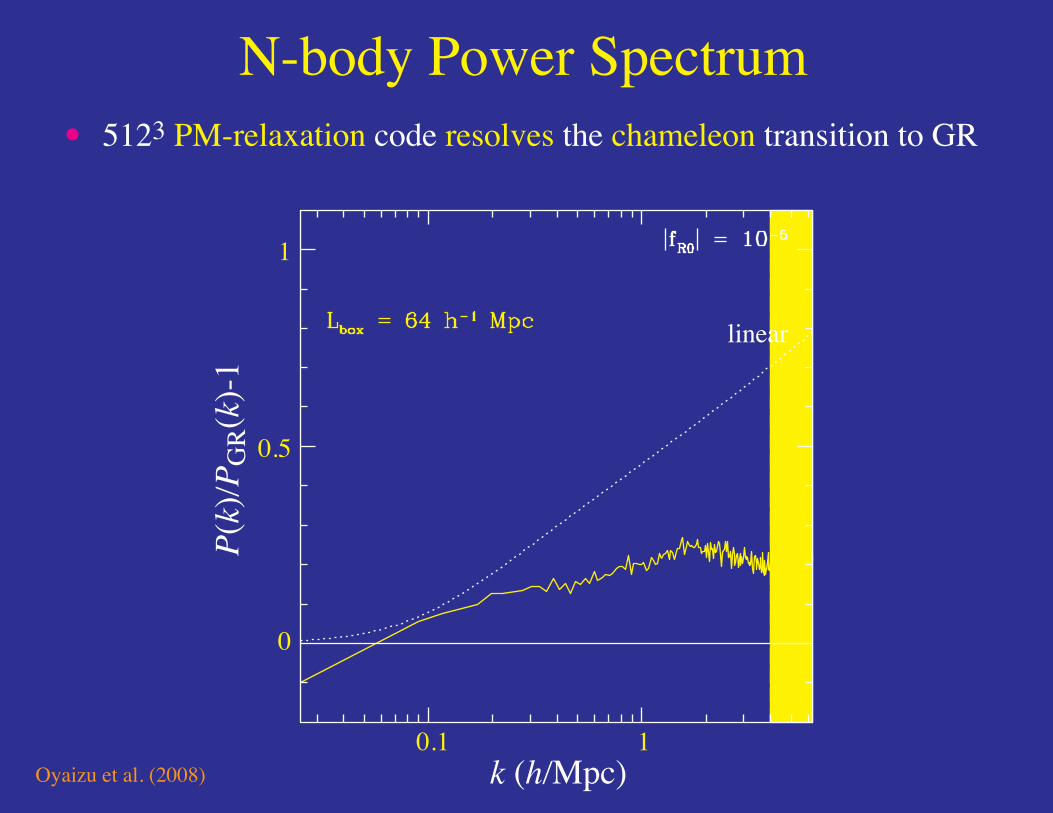
N-body Power Spectrum• 5123 PM-relaxation code resolves the chameleon transition to GR
Oyaizu et al. (2008) k (h/Mpc)
P(k)
/PG
R(k
)-1
0.1 1
0
1
0.5
linear

Hu, Huterer & Smith (2006)
4
N-body Power Spectrum• Chameleon transition weakens with higher field amplitude
Oyaizu et al. (2008) k (h/Mpc)
P(k)
/PG
R(k
)-1
0.1 1
0
1
0.5
linear

Three Regimes• Three regimes defined by γ=−Φ/Ψ BUT with different dynamics
• Examples f(R) and DGP braneworld acceleration
• Parameterized Post-Friedmann description
• Non-linear regime follows a halo paradigm but a full parameterization still lacking and theoretical, workable, examples few
Hu & Sawicki (2007)
r* rc
Scalar-TensorRegime
Conserved-CurvatureRegime
General RelativisticNon-Linear Regime
rhalos, galaxy large scale structure CMB

Summary• Model building requirements: mass squared positive and large at
high curvature with a small amplitude cosmological field
• Cosmological tests at very different range of curvature than localtests and worthwhile even in absence of viable full theory
• Strongest current constraint is from galaxy-ISW correlations inlinear regime - lack of anti-correlation rules out order unitybackground effects
• Solar system tests alone easy to evade but not in combination withfinite galaxy
• Requires cosmological simulations to study structure and evolutionof dark matter halos

Summary• N -body (PM-relaxation) simulations with non-linear chameleon
mechanism show strongest deviations at intermediate scales
• Lessons from f(R) and DGP braneworld examples:
3 regimes:
• large scales: conservation determined
• intermediate scales: scalar-tensor
• small scales: non-linear or GR
• Large and intermediate scales parameterized by metric ratio γ org = (Φ + Ψ)/(Φ−Ψ) as in PPN
• Additional 2 functions describing the large and intermediate scalerelationships to matter
• Small scales: non-linear mechanism and modified halo model


![Weak Lensing and Dark Energy Cosmology Tong-Jie Zhang[ 张同杰 ] Department of Astronomy, Beijing Normal University Cosmology Workshop Institute of High Energy](https://img.pdfslide.tips/doc/110x75/56649f575503460f94c7c2d3/weak-lensing-and-dark-energy-cosmology-tong-jie-zhang-department.jpg)