Embed Size (px)
Citation preview
The Formation of Firms' Inflation
Expectations: A Survey Data Analysis
Haruhiko Inatsugu * [email protected]
Tomiyuki Kitamura * [email protected]
Taichi Matsuda * [email protected]
No.19-E-15
November 2019
Bank of Japan 2-1-1 Nihonbashi-Hongokucho, Chuo-ku, Tokyo 103-0021, Japan
* Monetary Affairs Department
Papers in the Bank of Japan Working Paper Series are circulated in order to stimulate discussion
and comments. Views expressed are those of authors and do not necessarily reflect those of
the Bank.
If you have any comment or question on the working paper series, please contact each author.
When making a copy or reproduction of the content for commercial purposes, please contact the
Public Relations Department ([email protected]) at the Bank in advance to request
permission. When making a copy or reproduction, the source, Bank of Japan Working Paper
Series, should explicitly be credited.
Bank of Japan Working Paper Series
The Formation of Firms�In�ation Expectations:
A Survey Data Analysis�
Haruhiko Inatsuguy, Tomiyuki Kitamuraz, and Taichi Matsudax
November 2019
Abstract
In this paper, using both semi-aggregate and �rm-level survey data of the in�a-
tion expectations of Japanese �rms, we examine the empirical validity of three
hypotheses on the formation of in�ation expectations: the full-information rational
expectations (FIRE), noisy information, and sticky information hypotheses. Our
main �ndings are as follows. First, the results of our panel VAR analysis using
semi-aggregate data show that, while �rms�in�ation expectations have a forward-
looking aspect consistent with FIRE, they are not fully consistent with FIRE in
that they tend to incorporate the changes in the actual in�ation rate only gradu-
ally. Second, the forecast errors of semi-aggregate in�ation expectations correlate
with the past revisions of expectations, implying that FIRE does not hold for all
�rms. Third, the results of �rm-level dynamic panel regressions show that �rms�
in�ation expectations depend to a great extent on their past expectations, which
is consistent with both the noisy information and sticky information hypotheses.
The regression results also show that the short-term expectations of small �rms are
in�uenced by their perception of their own business conditions, which is consistent
with the noisy information hypothesis, especially the rational inattention variant.
These �ndings suggest that �rms in Japan form their in�ation expectations in a
complex manner that cannot be described by a single theory.
JEL Classi�cation: D84; E31; E52
Keywords: Firms�in�ation expectations; Survey data; FIRE; Noisy information; Sticky
information
�The authors are grateful to the sta¤ at the Bank of Japan, especially Kouki Inamura, Jouchi Naka-jima, Kenji Nishizaki, Tatsushi Okuda, and Masaki Tanaka, for helpful comments and discussions. Allremaining errors are our own. The views expressed in this paper are those of the authors and do notnecessarily re�ect the o¢ cial views of the Bank of Japan.
yMonetary A¤airs Department, Bank of Japan (E-mail: [email protected])zMonetary A¤airs Department, Bank of Japan (E-mail: [email protected])xMonetary A¤airs Department, Bank of Japan (E-mail: [email protected])
1
1 Introduction
In modern macroeconomics, �rms�in�ation expectations are one of the key determinants
of in�ation rates. In theory, as long as �rms have certain market power and incur some
costs (of any form) in changing their prices, as assumed in the New Keynesian Phillips
curve, changes in �rms�in�ation expectations have a crucial e¤ect on in�ation dynamics,
because �rms are the price-setters.
Current textbook macroeconomic models usually assume full-information rational ex-
pectations (FIRE) for the formation of �rms�in�ation expectations. However, there has
been skepticism over the empirical plausibility of FIRE, and recent empirical studies using
micro data point out its limited explanatory power (Coibion et al. 2018a).
As an alternative to FIRE, two hypotheses based on imperfect information have been
attracting particular attention in the recent literature.1 One of them is the noisy informa-
tion hypothesis, under which economic agents need to remove noise from the information
available, including the perception they have of their own business, and thus update their
expectations only gradually (Phelps 1970, Lucas 1972).2 The other is the sticky infor-
mation hypothesis, which assumes that economic agents do not necessarily update their
expectations every period due to the costs associated with acquiring new information
(Mankiw and Reis 2002, Reis 2006).
A number of empirical studies have examined the empirical validity of these hypothe-
ses using survey data of households� or professional forecasters� in�ation expectations.
However, there are relatively few empirical studies using survey data of �rms�in�ation
expectations. One reason is that, until recently, only a limited number of surveys on
in�ation expectations had been conducted covering a wide range of �rms.
In this paper, we use survey in�ation expectations of Japanese �rms to examine the
empirical validity of the three hypotheses mentioned above: the FIRE, noisy information
1There are also other hypotheses on expectations formation, e.g., the bounded rationality hypothesis(Sargent 1993, Gabaix 2014) and the adaptive learning hypothesis (Evans and Honkapohja 1999, 2001).Under these hypotheses, while agents have full information about macroeconomic variables, they haveonly imperfect information about the structure of the economy, and as a result their formation of in�ationexpectations deviates from FIRE. For more details of the various hypotheses on in�ation expectations,including those mentioned above, see the comprehensive survey by Coibion et al. (2018a).
2There are several variations and extensions of the noisy information hypothesis, such as the rationalinattention hypothesis (proposed by Sims 2003 and Mackowiak and Wiederholt 2009) and the higher-orderbelief hypothesis (proposed by Woodford 2003).
2
and sticky information hypotheses. The survey on in�ation expectations has been con-
ducted since 2014 as part of the Short-Term Economic Survey of Enterprises in Japan
(Tankan), which is carried out by the Bank of Japan and covers nearly 10,000 Japanese
�rms. We use both semi-aggregate and �rm-level data of the survey to examine the
hypotheses.
Our main �ndings are as follows. First, the results of our panel VAR analysis using
semi-aggregate data show that, while shocks to �rms�long-term expectations propagate
to their short-term expectations consistently with FIRE, �rms� in�ation expectations
are not fully consistent with FIRE in that they tend to incorporate the changes in the
actual in�ation rate only gradually. Second, the forecast errors of semi-aggregate in�ation
expectations correlate with the past revisions of expectations, implying a rejection of the
null hypothesis that FIRE holds for all �rms. Third, the results of �rm-level dynamic
panel regressions show that �rms� in�ation expectations depend to a great extent on
their past expectations, which is consistent with both the noisy information and sticky
information hypotheses. The regression results also show that the short-term expectations
of small �rms are in�uenced by their perception of their own business conditions, which
is consistent with the noisy information hypothesis, especially the rational inattention
variant. These �ndings suggest that �rms in Japan form their in�ation expectations in a
complex manner that cannot be described by a single theory.
Our results are consistent with those reported by a gradually increasing number of
empirical studies on the formation of �rms�in�ation expectations using survey data. For
instance, one of the papers by Coibion and Gorodnichenko (2015), who are leading the
research in this area, examines the correlation between forecast errors and past revisions
in aggregate in�ation expectations of various economic agents in the U.S., and reports
that FIRE is discon�rmed by the data, while both the noisy information and sticky
information hypotheses are supported. Adopting similar empirical approaches, Boneva
et al. (2016) and Richards and Verstraete (2016) report discon�rmation of FIRE for the
survey in�ation expectations of U.K. manufacturing �rms and Canadian �rms respectively.
Also, several empirical studies report that �rms� in�ation expectations are a¤ected by
their own business conditions, as the noisy information hypothesis suggests. Coibion et
al. (2018b) and Kumar et al. (2015) examine �rm-level data obtained from surveys that
3
they conducted with New Zealand �rms, and point out that �rms�in�ation expectations
are a¤ected by price developments and competition in their own industries, as well as
by the actual in�ation rate. Furthermore, the study of Richards and Verstraete (2016)
mentioned above also reports that �rms� in�ation expectations are in�uenced by �rm-
speci�c factors, such as their perception of labor shortages and their outlook for wages
and input prices, as well as macroeconomic conditions such as oil prices.
In Japan, the number of empirical studies on �rms�in�ation expectations has been
increasing. In particular, since the survey on in�ation expectations was launched as a
part of the Tankan in 2014, several empirical studies have examined the large panel
data of around 10,000 �rms. Uno et al. (2018) analyze the frequency of revisions of
in�ation expectations using the Tankan data, and report that the formation of �rms�
in�ation expectations is consistent with the sticky information hypothesis. Inamura et
al. (2017) and Economic Analysis Group of the Bank of Japan (2017) apply machine
learning techniques to the Tankan data, and report that the �rms�in�ation expectations
are a¤ected by �rm-speci�c information such as their own input prices, as well as by
macroeconomic information such as oil prices. Besides the studies using the Tankan
data, Kaihatsu and Shiraki (2016) use �rm-level data of the Annual Survey of Corporate
Behavior (conducted by the Economic and Social Research Institute of the Cabinet O¢ ce)
to analyze publicly-listed �rms�in�ation expectations (in terms of the GDP de�ator), and
report that in�ation expectations for shorter horizons tend to be a¤ected by their own
outlook for input prices and foreign exchange rates.
Compared with these previous studies, the main feature of this paper is its use of both
semi-aggregate and �rm-level data to examine the formation of �rms�in�ation expecta-
tions from several di¤erent perspectives. Another feature is its explicit inclusion of the
noisy information hypothesis in the scope of hypotheses to be examined in the empirical
analysis. One of its main contributions to the literature is to o¤er empirical evidence
supporting the noisy information hypothesis as well as the sticky information hypothesis
from the results of �rm-level panel data analysis.
The rest of the paper is organized as follows. Section 2 describes the Tankan data
we use in this paper. Section 3 examines the empirical validity of FIRE, using semi-
aggregate data. Section 4 examines the empirical validity of the noisy information and
4
sticky information hypotheses by conducting a dynamic panel regression analysis on �rm-
level data. Section 5 concludes.
2 Data
In this paper, we use the data of in�ation expectations ("outlook for general prices") and
judgment survey items of the Tankan. This section describes these data.
The Tankan is a statistical survey of private enterprises in Japan that is conducted by
the Bank of Japan on a quarterly basis (March, June, September, and December for each
year). The population of the survey is private enterprises in Japan (excluding �nancial
institutions) with capital of 20 million yen or more, according to the Economic Census
conducted by the Ministry of Internal A¤airs and Communications and the Ministry of
Economy, Trade and Industry.3 Sample enterprises are selected for each stratum of the
population divided by industry and size. As of March 2019, the total number of the
sample enterprises is 9,830 (1,922 large enterprises, 2,751 medium-sized enterprises and
5,157 small enterprises).4
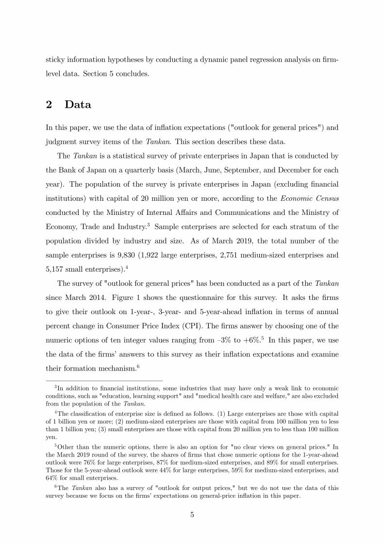
The survey of "outlook for general prices" has been conducted as a part of the Tankan
since March 2014. Figure 1 shows the questionnaire for this survey. It asks the �rms
to give their outlook on 1-year-, 3-year- and 5-year-ahead in�ation in terms of annual
percent change in Consumer Price Index (CPI). The �rms answer by choosing one of the
numeric options of ten integer values ranging from �3% to +6%.5 In this paper, we use
the data of the �rms�answers to this survey as their in�ation expectations and examine
their formation mechanism.6
3In addition to �nancial institutions, some industries that may have only a weak link to economicconditions, such as "education, learning support" and "medical health care and welfare," are also excludedfrom the population of the Tankan.
4The classi�cation of enterprise size is de�ned as follows. (1) Large enterprises are those with capitalof 1 billion yen or more; (2) medium-sized enterprises are those with capital from 100 million yen to lessthan 1 billion yen; (3) small enterprises are those with capital from 20 million yen to less than 100 millionyen.
5Other than the numeric options, there is also an option for "no clear views on general prices." Inthe March 2019 round of the survey, the shares of �rms that chose numeric options for the 1-year-aheadoutlook were 76% for large enterprises, 87% for medium-sized enterprises, and 89% for small enterprises.Those for the 5-year-ahead outlook were 44% for large enterprises, 59% for medium-sized enterprises, and64% for small enterprises.
6The Tankan also has a survey of "outlook for output prices," but we do not use the data of thissurvey because we focus on the �rms�expectations on general-price in�ation in this paper.
5
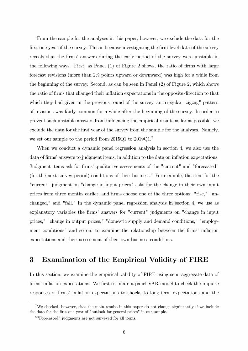
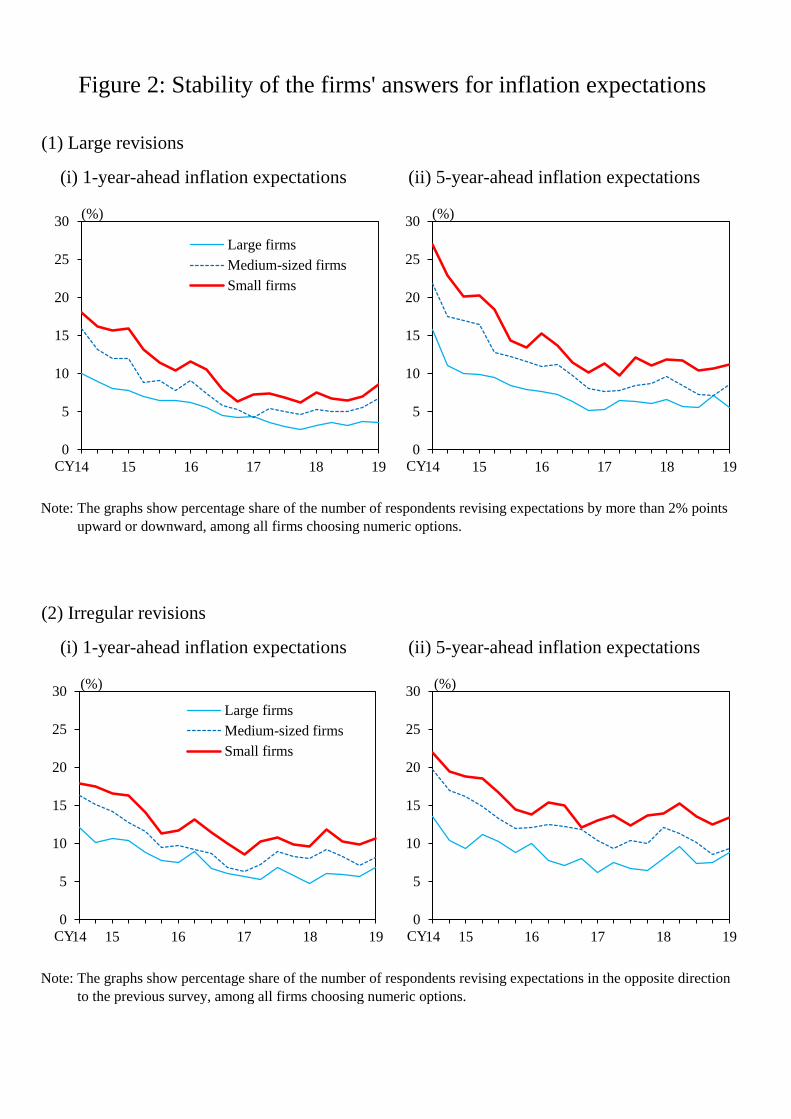
From the sample for the analyses in this paper, however, we exclude the data for the
�rst one year of the survey. This is because investigating the �rm-level data of the survey
reveals that the �rms�answers during the early period of the survey were unstable in
the following ways. First, as Panel (1) of Figure 2 shows, the ratio of �rms with large
forecast revisions (more than 2% points upward or downward) was high for a while from
the beginning of the survey. Second, as can be seen in Panel (2) of Figure 2, which shows
the ratio of �rms that changed their in�ation expectations in the opposite direction to that
which they had given in the previous round of the survey, an irregular "zigzag" pattern
of revisions was fairly common for a while after the beginning of the survey. In order to
prevent such unstable answers from in�uencing the empirical results as far as possible, we
exclude the data for the �rst year of the survey from the sample for the analyses. Namely,
we set our sample to the period from 2015Q1 to 2019Q1.7
When we conduct a dynamic panel regression analysis in section 4, we also use the
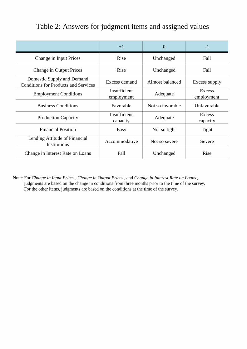
data of �rms�answers to judgment items, in addition to the data on in�ation expectations.
Judgment items ask for �rms�qualitative assessments of the "current" and "forecasted"
(for the next survey period) conditions of their business.8 For example, the item for the
"current" judgment on "change in input prices" asks for the change in their own input
prices from three months earlier, and �rms choose one of the three options: "rise," "un-
changed," and "fall." In the dynamic panel regression analysis in section 4, we use as
explanatory variables the �rms� answers for "current" judgments on "change in input
prices," "change in output prices," "domestic supply and demand conditions," "employ-
ment conditions" and so on, to examine the relationship between the �rms� in�ation
expectations and their assessment of their own business conditions.
3 Examination of the Empirical Validity of FIRE
In this section, we examine the empirical validity of FIRE using semi-aggregate data of
�rms�in�ation expectations. We �rst estimate a panel VAR model to check the impulse
responses of �rms� in�ation expectations to shocks to long-term expectations and the
7We checked, however, that the main results in this paper do not change signi�cantly if we includethe data for the �rst one year of "outlook for general prices" in our sample.
8"Forecasted" judgments are not surveyed for all items.
6
actual in�ation rate and discuss the consistency between the results and FIRE. We then
examine whether FIRE alone can explain the formation of �rms�in�ation expectations
with a statistical test on the forecast errors of �rms�in�ation expectations.
3.1 Examination Using Panel VAR
If �rms formed their in�ation expectations in accordance with FIRE, they would make
full use of available information about the economy to forecast in�ation rates. In this
case, �rms would form their in�ation expectations in a forward-looking manner, taking
into account, in particular, the long-term outlook for in�ation rates. Hence, if in�ation
expectations at longer horizons rose due to a change in the longer-term outlook for in�ation
rates, this would also a¤ect short-term in�ation expectations.
In addition, under FIRE, �rms on average would accurately forecast future in�ation
rates. Therefore, if the actual in�ation rate changed unexpectedly, they would immedi-
ately revise their in�ation expectations to correctly incorporate the subsequent dynamics
of in�ation rates.
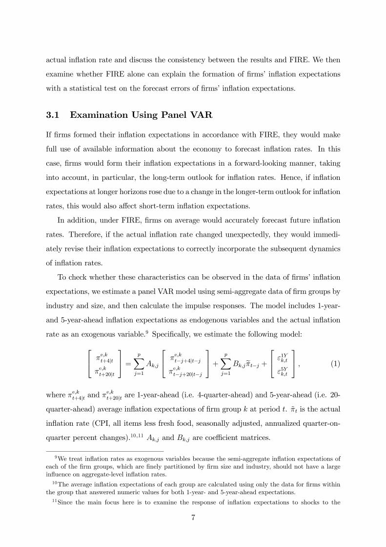
To check whether these characteristics can be observed in the data of �rms�in�ation
expectations, we estimate a panel VAR model using semi-aggregate data of �rm groups by
industry and size, and then calculate the impulse responses. The model includes 1-year-
and 5-year-ahead in�ation expectations as endogenous variables and the actual in�ation
rate as an exogenous variable.9 Speci�cally, we estimate the following model:24 �e;kt+4jt
�e;kt+20jt
35 = pXj=1
Ak;j
24 �e;kt�j+4jt�j
�e;kt�j+20jt�j
35+ pXj=1
Bk;je�t�j +24 "1Yk;t"5Yk;t
35 ; (1)
where �e;kt+4jt and �e;kt+20jt are 1-year-ahead (i.e. 4-quarter-ahead) and 5-year-ahead (i.e. 20-
quarter-ahead) average in�ation expectations of �rm group k at period t. ~�t is the actual
in�ation rate (CPI, all items less fresh food, seasonally adjusted, annualized quarter-on-
quarter percent changes).10 ;11 Ak;j and Bk;j are coe¢ cient matrices.
9We treat in�ation rates as exogenous variables because the semi-aggregate in�ation expectations ofeach of the �rm groups, which are �nely partitioned by �rm size and industry, should not have a largein�uence on aggregate-level in�ation rates.10The average in�ation expectations of each group are calculated using only the data for �rms within
the group that answered numeric values for both 1-year- and 5-year-ahead expectations.11Since the main focus here is to examine the response of in�ation expectations to shocks to the
7
In the estimation, we use the panel data of in�ation expectations of 93 �rm groups,
which are strati�ed based on the 3 �rm sizes (large, medium-sized, and small) and the 31
industry classi�cations used in the Tankan. The ordering of the Cholesky decomposition
for VAR is such that 5-year-ahead expectations are placed before 1-year-ahead expecta-
tions.12 The order of lag, p, is set to 2, based on the information criteria proposed by
Andrews and Lu (2001). The sample period is from 2015Q1 to 2019Q1.
Figure 3 shows the impulse responses to a +1% point shock in 5-year-ahead in�ation
expectations, whereas Figure 4 shows the impulse responses to a +1% point shock in the
actual in�ation rate.13
The result of Figure 3 indicates that there is a statistically signi�cant rise in 1-year-
ahead in�ation expectations following the rise in 5-year-ahead in�ation expectations. This
result implies that the formation of �rms� in�ation expectations has a forward-looking
aspect in the sense that �rms take into account the long-term outlook for in�ation rates
in forming their short-term in�ation expectations. This is consistent with FIRE.
On the other hand, �rms� in�ation expectations have a feature that is not consis-
tent with FIRE. The impulse responses of in�ation expectations to a positive shock to
the actual in�ation rate shown in Figure 4 indicate that, while the actual in�ation rate
monotonically declines after its immediate rise on impact, 1-year- and 5-year-ahead ex-
pectations only gradually increase and reach their peak with lags of one year or more.
As such, the formation of �rms�in�ation expectations has a tendency to incorporate the
changes in the actual in�ation rate only gradually.14 If the formation of �rms�in�ation
expectations were fully consistent with FIRE, �rms would on average accurately forecast
underlying factors of in�ation (not transient factors), we use "CPI (all items less fresh food)" in calculatingthe in�ation rate. The impulse responses do not change signi�cantly if we use "CPI (all items)" instead.12The results do not change qualitatively if we change the ordering of the Cholesky decomposition, or
if we employ the method of generalized impulse responses.13Impulse responses to the shock in the actual in�ation rate are calculated as follows. First, we estimate
an AR(2) model for the actual in�ation rate to capture its dynamics using the data from 1990Q1 to2019Q1. Next, we calculate the impulse responses of the actual in�ation rate by putting a +1% pointshock into the AR(2) model. Then we plug them into the terms of the actual in�ation rate in equation(1) to calculate the impulse responses of in�ation expectations.14Several works have shown that in�ation expectations in Japan tend to only gradually incorporate
the changes in the actual in�ation rate. For example, Bank of Japan (2018) points out such a tendencyfor professional in�ation forecasts, and Maruyama and Suganuma (2019) report similar results usinga compound index of in�ation expectations constructed using various survey and market data. Basedon these results, they argue that in�ation expectations in Japan are strongly a¤ected by the adaptiveformation mechanism.
8
the actual in�ation rate, and thus their in�ation expectations would immediately rise on
impact and decline monotonically afterwards, as the actual in�ation rate does. Hence,
the fact that in�ation expectations only gradually incorporate the changes in the actual
in�ation rate implies that the formation of �rms�in�ation expectations has an aspect that
cannot be described solely by FIRE.
3.2 Examination Based on Forecast Errors
The results in the previous subsection suggest that, although the formation of Japanese
�rms�in�ation expectations has a forward-looking aspect, its mechanism cannot be de-
scribed solely by FIRE. In this subsection, employing a framework proposed by Coibion
and Gorodnichenko (2015), we statistically test whether FIRE alone can explain the for-
mation of �rms�in�ation expectations.
In the testing framework proposed by Coibion and Gorodnichenko (2015), the empiri-
cal validity of FIRE is examined by testing whether the forecast errors of aggregate-level
in�ation expectations correlate with their past revisions. The reason why the empirical
validity of FIRE can be tested by checking the correlation is as follows. If all �rms, as
FIRE presupposes, make full use of all the observable information in forming their expec-
tations for the 1-year-ahead (year-on-year) in�ation rate �t+4, the in�ation expectation
of each �rm equals the mathematical expectation of the in�ation rate conditional on the
information at period t, i.e. Et�t+4, and thus the average in�ation expectation of the
�rms also equals this value. In this case, theoretically, the aggregate-level forecast error
of in�ation expectations, �t+4 � Et�t+4, should not correlate with any variables that are
observable at period t.15 Hence, if the forecast error correlates with the revision of in�a-
tion expectations made at period t, which is obviously observable at period t, it follows
that FIRE does not hold for all �rms.
In this subsection, following Coibion and Gorodnichenko (2015), we examine the corre-
lation between the forecast errors and the revisions of in�ation expectations by estimating
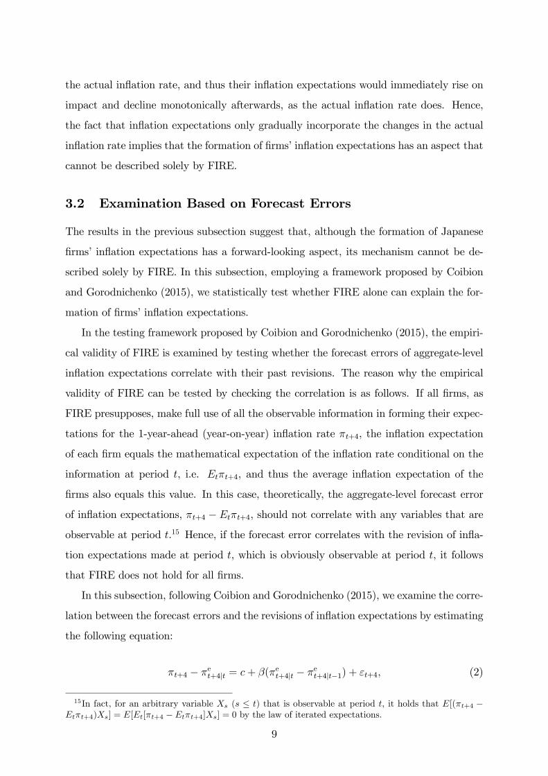
the following equation:
�t+4 � �et+4jt = c+ �(�et+4jt � �et+4jt�1) + "t+4; (2)
15In fact, for an arbitrary variable Xs (s � t) that is observable at period t, it holds that E[(�t+4 �Et�t+4)Xs] = E[Et[�t+4 � Et�t+4]Xs] = 0 by the law of iterated expectations.
9
where �t+4 is the actual in�ation rate one year after period t (CPI, all items, year-on-
year percent change), and �et+4jt is the average of the 1-year-ahead (i.e. 4-quarter-ahead)
in�ation expectations that are formed at period t.16 Hence the left-hand side of the
equation is the forecast error of 1-year-ahead in�ation expectations, whereas the term
in parentheses on the right-hand side of the equation is the revision (from the previous
quarter to the current quarter) of 1-year-ahead in�ation expectations.17
The coe¢ cient � in equation (2) is zero (that is, the forecast error and the revision are
uncorrelated) if and only if FIRE holds for all �rms. Therefore, if � = 0 is rejected in the
estimation results of equation (2), indicating the forecast error and the forecast revision
are correlated, then the null hypothesis that "FIRE holds for all �rms" is rejected.
We could set up equations similar to equation (2) for 3-year- and 5-year-ahead in�ation
expectations as well. However, because the Tankan data of in�ation expectations are
relatively short in the time series dimension, the number of observations of the forecast
errors on the left-hand side of the equations would be very limited for 3-year- and 5-year-
ahead in�ation expectations. Therefore, here we focus the analysis only on 1-year-ahead
expectations.
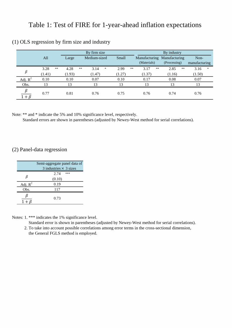
Panel (1) of Table 1 shows the estimation results of equation (2) for each of 9 industry-
size groups (3 industry groups and 3 size groups; 9 industry-size groups in total), using 1-
year-ahead average in�ation expectations.18 The sample period is from 2015Q1 to 2019Q1.
For all groups, the estimates of � are statistically signi�cant, and thus the null hypothesis
of � = 0 is rejected. This result implies that FIRE does not in general hold for the
formation of �rms�in�ation expectations.
However, the estimation results for each industry-size group may not necessarily be
su¢ ciently reliable, because the number of observations is limited to 13 in these cases.
To complement this, we also estimate equation (2) with panel data of the 9 industry-size
groups (i.e. the cross-sectional dimension is 9). Panel (2) of Table 1 shows the result of
16We use "CPI (all items)" here because the Tankan does not ask the �rms to exclude any speci�citems such as fresh food in giving their in�ation expectations.17In the Tankan, since the forecast horizons are �xed at 1 year (4 quarters), 3 years (12 quarters), and
5 years (20 quarters), the data corresponding to �et+4jt�1 (the 5-quarter-ahead forecast in period t � 1)on the right-hand side of equation (2) does not exist. In this paper, we use the data corresponding to�et+3jt�1 (the 4-quarter-ahead forecast in period t� 1) in place of �et+4jt�1.18We checked that none of the estimates of constant c, which are omitted in the table, are statistically
signi�cant.
10
the panel-data regression.19 The estimate of � is again statistically signi�cant, and the
null hypothesis of � = 0 is rejected in this case as well.
These results indicate that, on average, FIRE is not empirically valid for the �rms�
in�ation expectations. Of course, this does not deny the possibility that FIRE can cor-
rectly describe the formation of in�ation expectations by some of the �rms. However, the
results in this subsection, as well as the results of the panel VAR in the previous subsec-
tion, strongly suggest that the mechanism of the formation of �rms�in�ation expectations
cannot be described solely by FIRE.
Then, what other hypotheses can explain the formation of �rms� in�ation expecta-
tions? In this regard, Coibion and Gorodnichenko (2015) show that � in equation (2) is
positive under either the noisy information hypothesis or the sticky information hypoth-
esis. Their argument is as follows. First, under the noisy information hypothesis, �rms
take account of the fact that observed data of the in�ation rate contain noise, and they
update only some fraction G (0 < G < 1) of their expectations using the information
contained in the in�ation rate, while they keep the remaining fraction 1 � G of their
expectations unchanged from the previous period. In this case, the average forecast error
of in�ation expectations can be written as
�t+4 � �et+4jt =1�GG
(�et+4jt � �et+4jt�1) + �t+4; (3)
where �t+4 is an error term. Second, under the sticky information hypothesis, a fraction
1 � � of �rms update their information and revise their expectations by making full use
of it, whereas the remaining fraction � of �rms keep their expectations unchanged from
the previous period. In this case, the average forecast error of in�ation expectations can
be written as
�t+4 � �et+4jt =�
1� �(�et+4jt � �et+4jt�1) + �t+4: (4)
19To be more speci�c, the equation for the panel-data regression is as follows:
�t+4 � �e;it+4jt = i + �(�e;it+4jt � �
e;it+4jt�1) + "i;t+4;
where i is an index for industry-size group, and the error term "i;t+4 captures factors other than therevision of expectations (�e;it+4jt � �
e;it+4jt�1) and �xed e¤ects ( i) that a¤ect forecast errors. Because the
forecast errors can be correlated with each other across the cross-sectional dimension, for this panel-dataregression we employ General FGLS to take into account possible cross-sectional correlations betweenthe error terms. For details of General FGLS, see Wooldridge (2010, Chapter 10).
11
Hence, the result shown in Table 1 that � is positive to a statistically signi�cant extent
suggests that either the noisy information hypothesis or the sticky information hypothesis
may be empirically valid.
Furthermore, using the estimate of �, we can quantify the degree of information rigidity
due to noisy information or sticky information. That is, comparing equation (2) with
equations (3) and (4) reveals that both 1�G, which is the weight that �rms place on the
previous period�s expectations under the noisy information hypothesis, and �, which is
the fraction of �rms that keep their expectations unchanged under the sticky information
hypothesis, correspond to �=(1 + �). Therefore, under either hypothesis, the degree of
information rigidity can be measured with �=(1 + �).
The value of �=(1+�) for each estimate of � is shown in the bottom row of each panel
in Table 1. For instance, the value calculated using the estimate of � obtained by the
panel-data regression is 0.73. From the viewpoint of the noisy information hypothesis, this
implies that �rms incorporate only 27% (= 100% �73%) of newly acquired information
into their in�ation expectations because of the presence of noise in the information. Or,
from the viewpoint of the sticky information hypothesis, this implies that in each period
only 27% of the �rms revise their expectations. Regarding the latter, Figure 5 shows the
frequency of revisions of in�ation expectations for our sample data, calculated in the same
way as that of Uno et al. (2018) whose sample period is from March 2014 to September
2017. The frequency for 1-year-ahead in�ation expectations is 4 out of 16 during the
sample period. This is consistent with the result based on the estimate of � which we
mentioned above.20
These results of the examination based on the forecast errors suggest that the noisy
information hypothesis and the sticky information hypothesis are likely to be empiri-
cally valid for the formation of �rms�in�ation expectations. In the next section, we use
�rm-level data of in�ation expectations to examine the empirical validity of these two
hypotheses.
20The fact that a �rm does not revise its in�ation expectations does not necessarily mean that the�rm does not update its information set. Even when a �rm updates its information set, it can keep itsexpectations unchanged if the new information simply con�rms its expectations. Therefore, the frequencyof revisions of in�ation expectations discussed here should be interpreted as a lower bound of the frequencyof information updates.
12
4 Examination of the Empirical Validity of the Noisy
Information and Sticky Information Hypotheses
In this section, we examine the empirical validity of the noisy information and sticky
information hypotheses via a dynamic panel regression analysis of �rm-level data. In
doing so, we �rst explore what features �rm-level data of in�ation expectations would
exhibit under these hypotheses, and then set up an empirical framework that can capture
such features. After that, we discuss the estimation results.
4.1 Implications of Noisy Information and Sticky Information
Hypotheses on Firm-Level Data
In exploring what features would appear in the �rm-level data of in�ation expectations
under the noisy information and sticky information hypotheses, we assume that the econ-
omy can be represented by the following model with a relatively simple structure.
�t = AX�t + �
�t ; (5)
X�t = BX
�t�1 + �
Xt ; (6)
where �t denotes the in�ation rate, X�t other macroeconomic variables, �
�t a shock to the
in�ation rate, and �Xt shocks to the macroeconomic variables excluding the in�ation rate.
A and B are coe¢ cient matrices.
4.1.1 Noisy Information Hypothesis
Under the noisy information hypothesis, �rms extract information that is useful for form-
ing their in�ation expectations not only from information on macroeconomic conditions
but also from �rm-speci�c information such as the purchase price of raw materials. Below,
we show this by using a model that extends the model of Coibion and Gorodnichenko
(2015). Appendix contains details of the derivations of the key equation and related
discussions.
Assume that �rms cannot observe the macroeconomic variables X�t directly, and that
13
they can only observe the macroeconomic indices Xt that contain noise "Xt as follows.21
Xt = X�t + "
Xt : (7)
Also, assume that the �rm i�s idiosyncratic variables Yi;t, such as input prices and
demand conditions the �rm faces, are driven by the macroeconomic variables X�t as well
as �rm-level shocks �Yi;t as follows.
Yi;t = CX�t + �
Yi;t; (8)
where C is a coe¢ cient matrix. Hence, the �rm�s idiosyncratic variables Yi;t also contain
information about the macroeconomic variables X�t .
Under this setting, a �rm has to estimate the unobservable macroeconomic variables
X�t using the observed macroeconomic indices Xt, the actual in�ation rate �t, and the
idiosyncratic variables Yi;t in predicting future in�ation rates.22 The Kalman �lter is
known to be the optimal way to make an estimate and a prediction in this environment.
The estimate of X�t obtained via the Kalman �lter is given by
Ei;tX�t = G
Xi;tXt +G
�i;t�t +G
Yi;tYi;t + (I �GXi;t)Ei;t�1X�
t �G�i;tEi;t�1�t �GYi;tEi;t�1Yi;t; (9)
where GXi;t, G�i;t, and G
Yi;t are matrices that represent the weights placed by �rm i on the
observable variablesXt, �t, and Yi;t, respectively, and Ei;t is the mathematical expectation
operator conditional on the information available to �rm i at period t.
Substituting equations (5) and (8) into the �fth and sixth terms in the right-hand side
of equation (9), multiplying both sides by ABh, and applying equations (5) and (6) yields
the following equation for h-period-ahead in�ation expectations:
Ei;t�t+h = (I �GXi;t �G�i;tA�GYi;tC)Ei;t�1�t+h + ABh(GXi;tXt +G�i;t�t +G
Yi;tYi;t): (10)
21In the seminal work on the noisy information hypothesis by Lucas (1972), noise in a macroeconomicvariable (nominal amount of money) is assumed to disappear in one period. In contrast, noise contained ineconomic variables does not completely disappear in our setting. Our setting is close to that of Woodford(2003), who extended Lucas�model.22Imagine, for example, a situation where the in�ation rate �t and the input prices Yi;t in �rm i�s
industy are both a¤ected by the output gap X�t , which cannot be observed directly and therefore has to
be estimated by the observed data (Xt, �t, Yi;t).
14
The implications we can draw from this equation, derived under the noisy information
hypothesis, are threefold. First, �rms�in�ation expectations (Ei;t�t+h) depend on their
own expectations formed in the previous period (Ei;t�1�t+h). Second, the �rms�in�ation
expectations are a¤ected by current macroeconomic information (Xt and �t).23 Third,
�rms�in�ation expectations are also a¤ected by their own idiosyncratic information (Yi;t).
In particular, under the rational inattention hypothesis, which is a variant of the noisy
information hypothesis, economic agents with limited capacity for information processing
focus their attention primarily on information useful for their own business, and therefore
�rms pay more attention to micro-level information Yi;t that directly a¤ects their business
than to macroeconomic information, Xt and �t.24
Hence, in order to capture the features of expectations formation that would be ex-
hibited under the noisy information hypothesis in a panel regression analysis, we should
include lagged in�ation expectations, macroeconomic variables, and �rm-speci�c variables
as explanatory variables in the regression.
It can also be seen from equation (10) that, if the macroeconomic variables X�t are
stationary, as the forecast horizon becomes longer (h becomes larger), Bh on the right-
hand side of the equation converges to the zero matrix, and thus the current variables,
including the �rm-speci�c variables, become less likely to in�uence in�ation expectations.
Therefore, even under the noisy information hypothesis, the estimates of the coe¢ cients
on current variables may not necessarily be statistically signi�cant for long-term in�ation
expectations.
4.1.2 Sticky Information Hypothesis
Under the sticky information hypothesis, because of the presence of the cost of informa-
tion updates, it can be optimal for �rms to leave their expectations unchanged without
acquiring new information relevant to forming expectations. The optimal behavior of a
�rm in such a situation is modeled by Reis (2006).25 In this model, a �rm facing the cost
23Past macroeconomic information indirectly a¤ects current in�ation expectations through the pastexpectations formed in the previous period (Ei;t�1�t+h).24Mackowiak and Wiederholt (2009) apply the rational inattention hypothesis to �rms�price setting
problem, and theoretically show that prices become less responsive to shocks in nominal demand as �rmsfocus their attention on micro-level information that directly a¤ects their own business.25In the seminal paper of Mankiw and Reis (2002), who proposed the sticky information hypothesis, a
certain fraction of �rms are assumed to leave their expectations unchanged, but the mechanism by which
15
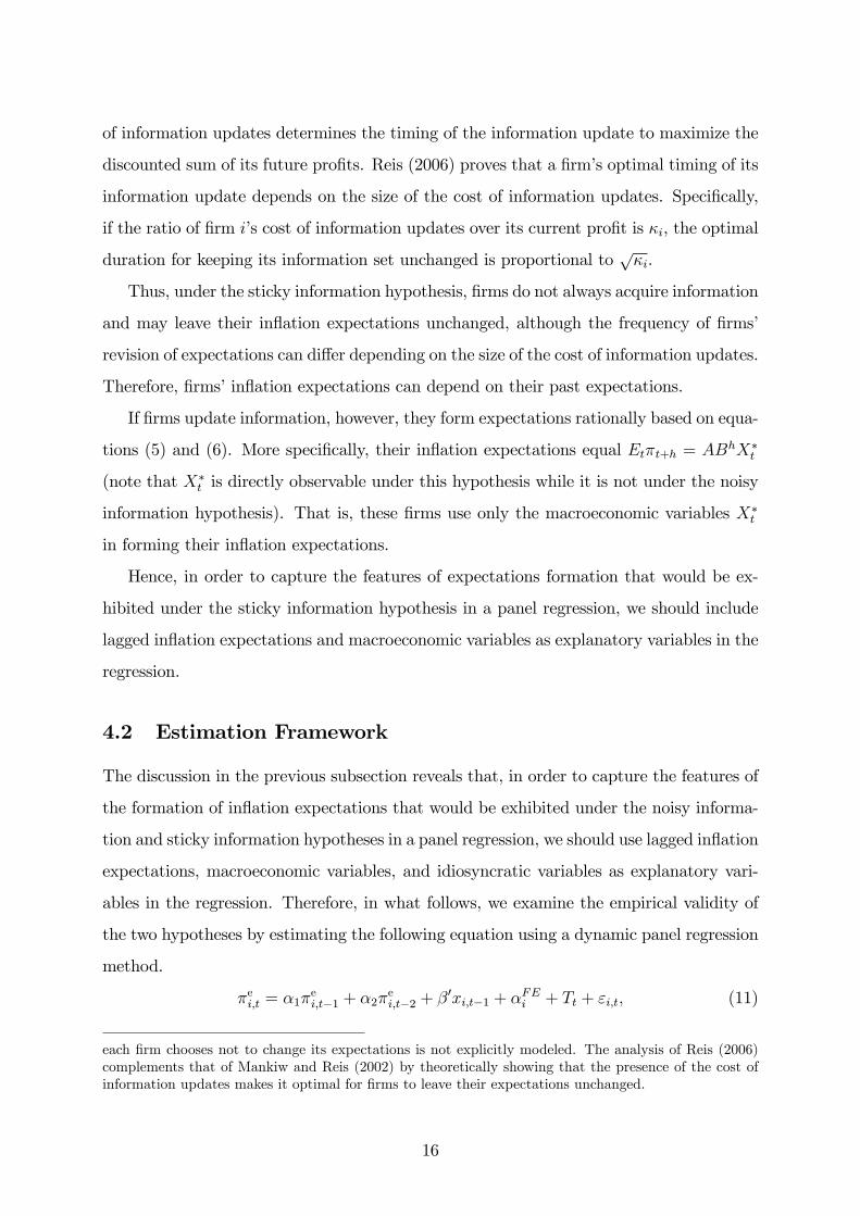
of information updates determines the timing of the information update to maximize the
discounted sum of its future pro�ts. Reis (2006) proves that a �rm�s optimal timing of its
information update depends on the size of the cost of information updates. Speci�cally,
if the ratio of �rm i�s cost of information updates over its current pro�t is �i, the optimal
duration for keeping its information set unchanged is proportional top�i.
Thus, under the sticky information hypothesis, �rms do not always acquire information
and may leave their in�ation expectations unchanged, although the frequency of �rms�
revision of expectations can di¤er depending on the size of the cost of information updates.
Therefore, �rms�in�ation expectations can depend on their past expectations.
If �rms update information, however, they form expectations rationally based on equa-
tions (5) and (6). More speci�cally, their in�ation expectations equal Et�t+h = ABhX�t
(note that X�t is directly observable under this hypothesis while it is not under the noisy
information hypothesis). That is, these �rms use only the macroeconomic variables X�t
in forming their in�ation expectations.
Hence, in order to capture the features of expectations formation that would be ex-
hibited under the sticky information hypothesis in a panel regression, we should include
lagged in�ation expectations and macroeconomic variables as explanatory variables in the
regression.
4.2 Estimation Framework
The discussion in the previous subsection reveals that, in order to capture the features of
the formation of in�ation expectations that would be exhibited under the noisy informa-
tion and sticky information hypotheses in a panel regression, we should use lagged in�ation
expectations, macroeconomic variables, and idiosyncratic variables as explanatory vari-
ables in the regression. Therefore, in what follows, we examine the empirical validity of
the two hypotheses by estimating the following equation using a dynamic panel regression
method.
�ei;t = �1�ei;t�1 + �2�
ei;t�2 + �
0xi;t�1 + �FEi + Tt + "i;t; (11)
each �rm chooses not to change its expectations is not explicitly modeled. The analysis of Reis (2006)complements that of Mankiw and Reis (2002) by theoretically showing that the presence of the cost ofinformation updates makes it optimal for �rms to leave their expectations unchanged.
16
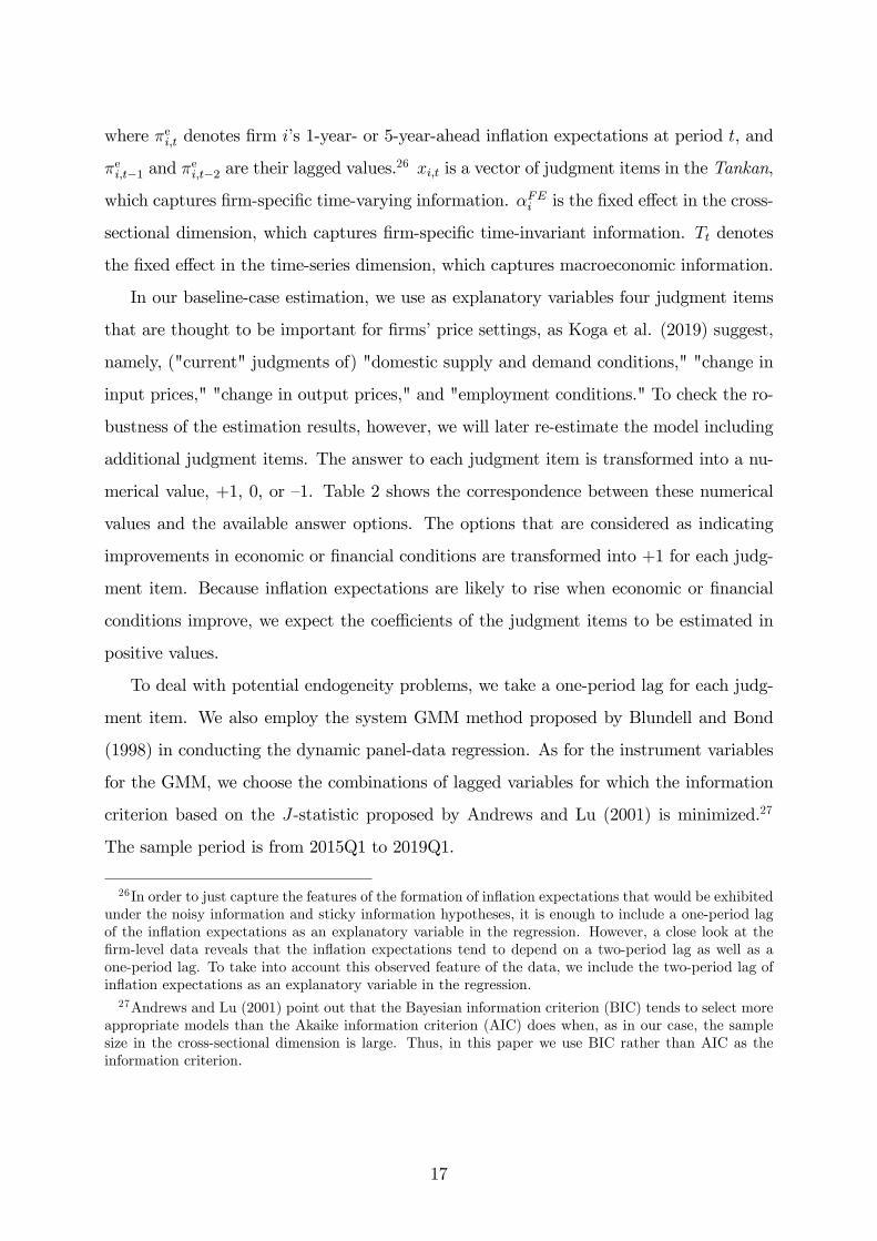
where �ei;t denotes �rm i�s 1-year- or 5-year-ahead in�ation expectations at period t, and
�ei;t�1 and �ei;t�2 are their lagged values.
26 xi;t is a vector of judgment items in the Tankan,
which captures �rm-speci�c time-varying information. �FEi is the �xed e¤ect in the cross-
sectional dimension, which captures �rm-speci�c time-invariant information. Tt denotes
the �xed e¤ect in the time-series dimension, which captures macroeconomic information.
In our baseline-case estimation, we use as explanatory variables four judgment items
that are thought to be important for �rms�price settings, as Koga et al. (2019) suggest,
namely, ("current" judgments of) "domestic supply and demand conditions," "change in
input prices," "change in output prices," and "employment conditions." To check the ro-
bustness of the estimation results, however, we will later re-estimate the model including
additional judgment items. The answer to each judgment item is transformed into a nu-
merical value, +1, 0, or �1. Table 2 shows the correspondence between these numerical
values and the available answer options. The options that are considered as indicating
improvements in economic or �nancial conditions are transformed into +1 for each judg-
ment item. Because in�ation expectations are likely to rise when economic or �nancial
conditions improve, we expect the coe¢ cients of the judgment items to be estimated in
positive values.
To deal with potential endogeneity problems, we take a one-period lag for each judg-
ment item. We also employ the system GMM method proposed by Blundell and Bond
(1998) in conducting the dynamic panel-data regression. As for the instrument variables
for the GMM, we choose the combinations of lagged variables for which the information
criterion based on the J-statistic proposed by Andrews and Lu (2001) is minimized.27
The sample period is from 2015Q1 to 2019Q1.
26In order to just capture the features of the formation of in�ation expectations that would be exhibitedunder the noisy information and sticky information hypotheses, it is enough to include a one-period lagof the in�ation expectations as an explanatory variable in the regression. However, a close look at the�rm-level data reveals that the in�ation expectations tend to depend on a two-period lag as well as aone-period lag. To take into account this observed feature of the data, we include the two-period lag ofin�ation expectations as an explanatory variable in the regression.27Andrews and Lu (2001) point out that the Bayesian information criterion (BIC) tends to select more
appropriate models than the Akaike information criterion (AIC) does when, as in our case, the samplesize in the cross-sectional dimension is large. Thus, in this paper we use BIC rather than AIC as theinformation criterion.
17
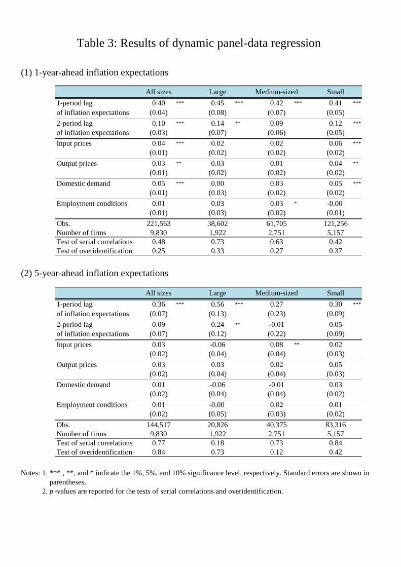
4.3 Estimation Results
Table 3 shows the estimation results of the baseline case with the four judgment items. For
both 1-year- and 5-year-ahead expectations, the estimated coe¢ cients on the lags of in�a-
tion expectations are statistically signi�cant, consistent with both the noisy information
and sticky information hypotheses.
On the other hand, for the judgment items, the results di¤er across time horizons of
in�ation expectations and �rm sizes. Below we will discuss the results by time horizons
of in�ation expectations.
4.3.1 1-Year-Ahead In�ation Expectations
As for 1-year-ahead in�ation expectations of small �rms, the estimated coe¢ cients on
input prices, output prices, and domestic demand are statistically signi�cant.28 This
result suggests the empirical validity of the noisy information hypothesis, especially of
the rational inattention hypothesis. In addition, as we expected, the coe¢ cients are
estimated to be positive. Our interpretations of the estimation results for the coe¢ cients
are as follows.
First, the reason why small �rms with rising input prices tend to have higher in�ation
expectations could be that small �rms extract information on price developments around
them from input prices and use the information in forming their in�ation expectations.
Second, small �rms with rising output prices also tend to have higher in�ation expectations
possibly because they think that, since they are able to (or forced to) raise output prices,
their competitors will also raise their prices, and expect that this will result in a rise in
the general price level. Third, small �rms that recognize excess demand in their domestic
markets have higher in�ation expectations probably because they think that the tight
demand in the markets will lead many �rms to raise their prices.
In contrast to the results for small �rms, none of the estimated coe¢ cients on the
judgment items are statistically signi�cant for large �rms. One possible interpretation of
this result is that the rational inattention hypothesis does not hold for large �rms, but
28Economic Analysis Group of the Bank of Japan (2017), who applied machine learning techniques tothe Tankan data to examine factors that a¤ect �rms�in�ation expectations, also report that 1-year-aheadin�ation expectations of �rms are a¤ected by their judgments regarding input prices, output prices, and�nancial position.
18
there are two other possible interpretations.
The �rst interpretation is actually based on the rational inattention hypothesis. Un-
der this hypothesis, �rms with limited capacity for information processing focus their
attention primarily on information that a¤ects their business, and they form their in-
�ation expectations using such information. Hence, if macroeconomic conditions have a
relatively large impact on their business, large �rms may not pay much attention to their
�rm-speci�c information while paying much more attention to macroeconomic informa-
tion. Based on this interpretation, the fact that the judgment items are not statistically
signi�cant for large �rms does not necessarily contradict the rational inattention hypoth-
esis (or the noisy information hypothesis that includes it as a variant), but rather can be
regarded as consistent with the rational inattention hypothesis.
The second interpretation is that the size of the cost of decision-making depends
on �rm size. As the empirical study by Zbaracki et al. (2004) suggests, a large �rm
may incur large costs for internal decision-making processes such as coordination among
internal divisions, and thus it can take a long time for the organization as a whole to
determine its in�ation expectations.29 Therefore, in a large �rm, even when its own
business conditions change, the person responsible for answering the Tankan survey may
have to leave the answer for in�ation expectations unchanged until the organization as a
whole determines its o¢ cial in�ation expectations.30 On the other hand, small �rms may
face smaller decision-making costs than large �rms do, making it easier for them to change
their in�ation expectations in a short period of time. Because of this, small �rms may be
able to change their answers for in�ation expectations in the survey (together with those
for the judgment items) more easily by taking into account the ongoing changes in their
business conditions.
29Zbaracki et al. (2004) conduct a case study on a large �rm in the U.S. According to the results, thecosts related to acquiring information and revising its economic forecasts (the total cost of informationgathering, decision-making, and internal communication) amount to 4.6% of their net pro�ts.30As we noted in footnote 5, for large �rms, the share of �rms that chose a numeric option for their
1-year-ahead expectation is 76%, which is lower than 87% for medium-sized �rms and 89% for small�rms (as of March 2019). In addition, as shown in Figure 5, the frequency of expectation revision oflarge �rms is lower than that of smaller �rms. These features of the data may also re�ect that the costsof decision-making increase as �rm size increases.
19
4.3.2 5-Year-Ahead Expectations
As for 5-year-ahead in�ation expectations, the estimated coe¢ cients on all judgment items
are statistically insigni�cant for both large and small �rms.31 This result may simply
re�ect the possibility that, in forming long-term in�ation expectations, �rms do not �nd
information on their current business conditions useful, due to the intrinsically high degree
of uncertainty about the long-term future. Indeed, as we discussed in Section 4, even under
the noisy information hypothesis, current variables may not be statistically signi�cant for
long-term in�ation expectations. Therefore, this result does not necessarily imply that
the noisy information hypothesis fails to hold for the �rms�in�ation expectations.
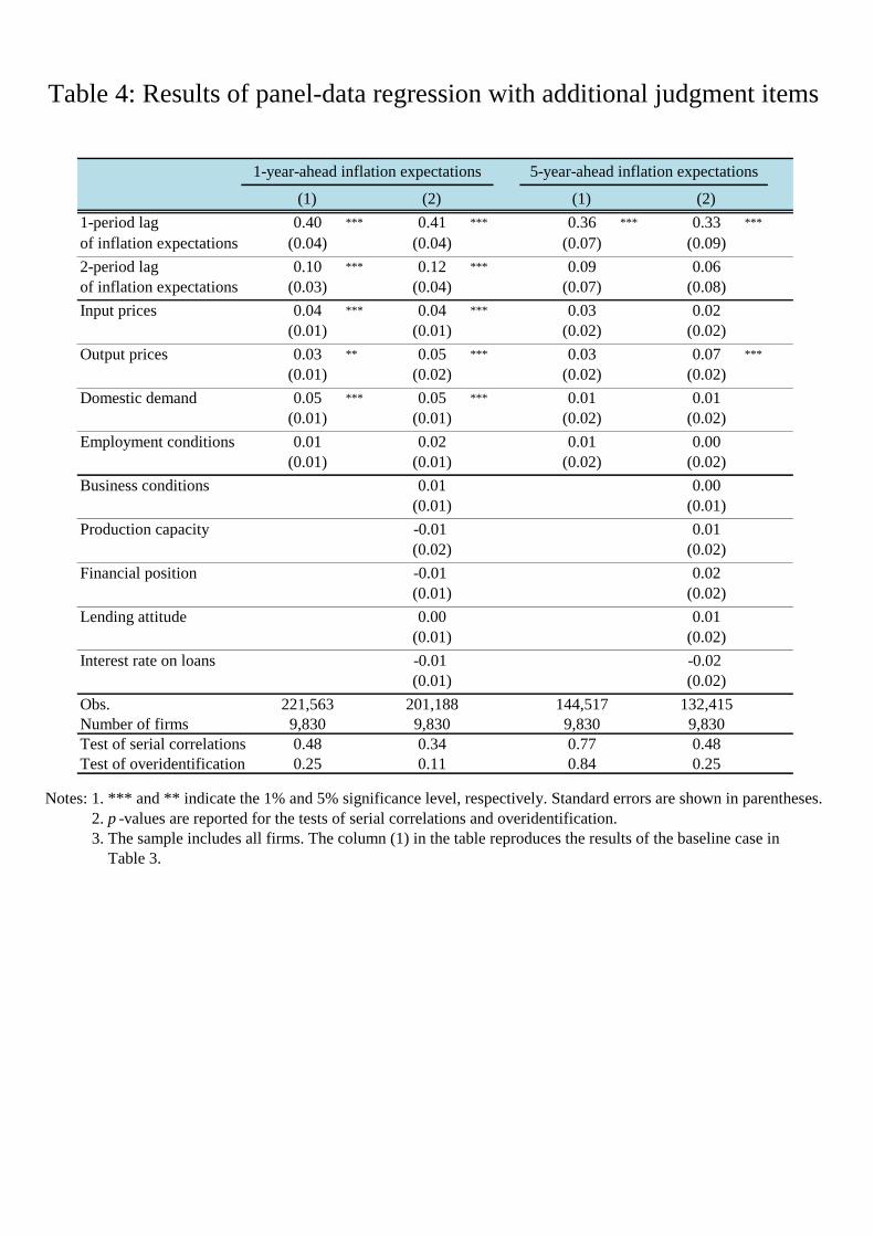
4.4 Robustness Check: the Case with Additional Judgment
Items
In the baseline case, we used as explanatory variables the four judgment items that are
thought to be important for �rms�price setting behavior. However, in forming their in-
�ation expectations, �rms might also use information that is contained in other judgment
items.
To check the robustness of the results of the baseline case with respect to this point,
we re-estimate the model including additional judgment items as explanatory variables,
using the data for all �rms. The additional items are ("current" judgments on) "business
conditions," "production capacity," "�nancial position," and "change in interest rate on
loans."32
Table 4 shows the estimation results of the case with the additional judgment items.
For both 1-year- and 5-year-ahead in�ation expectations, there is no dramatic change in
the values and statistical signi�cance of the estimated coe¢ cients on the lagged in�ation
expectations and the judgment items that were already used in the baseline case. In
addition, all of the estimated coe¢ cients on the additional judgment items are statistically
insigni�cant.
31Economic Analysis Group of the Bank of Japan (2017), who applied machine learning techniques tothe Tankan data, also report that judgment items do not have a large in�uence on long-term in�ationexpectations.32We do not use some judgment items such as "overseas supply and demand conditions" and "inventory
level of �nished goods and merchandise," for which the number of respondent �rms is limited.
20
Hence, we conclude that the four judgment items used in the baseline case capture
most of the information that �rms use in forming their in�ation expectations.
5 Conclusion
In this paper, using both semi-aggregate and �rm-level data of survey in�ation expecta-
tions of Japanese �rms, we examine the empirical validity of three hypotheses on in�ation
expectations formation: the FIRE, noisy information, and sticky information hypotheses.
Our main �ndings are as follows. First, the results of our panel VAR analysis using
semi-aggregate data show that, while shocks to �rms�long-term expectations propagate
to their short-term expectations consistently with FIRE, �rms� in�ation expectations
are not fully consistent with FIRE in that they tend to incorporate the changes in the
actual in�ation rate only gradually. Second, the forecast errors of semi-aggregate in�ation
expectations correlate with the past revisions of expectations, implying a rejection of the
null hypothesis that FIRE holds for all �rms. Third, the results of �rm-level dynamic
panel regressions show that �rms� in�ation expectations depend to a great extent on
their past expectations, which is consistent with both the noisy information and sticky
information hypotheses. The regression results also show that the short-term expectations
of small �rms are in�uenced by their perception of their own business conditions, which
is consistent with the noisy information hypothesis, especially the rational inattention
variant. These �ndings suggest that �rms in Japan form their in�ation expectations in a
complex manner that cannot be described by a single theory.
The conclusion of this paper that �rms�formation of in�ation expectations cannot be
described by a single theory provides an important suggestion as to how to build macro-
economic models that are consistent with the actual data of �rms�in�ation expectations.
An important topic for future research is to explore the implications for macroeconomic
dynamics of the various hypotheses on the formation of in�ation expectations, such as the
noisy information and sticky information hypotheses, by building macroeconomic mod-
els that incorporate these hypotheses to successfully explain the actual data of in�ation
expectations.33
33The paper by Kitamura and Tanaka (2019) is one example of recent work in this direction. Using thedata for Japan, including the aggregate in�ation expectations in the Tankan, they estimate a small-size
21
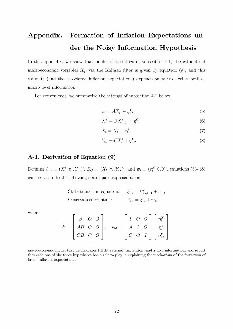
Appendix. Formation of In�ation Expectations un-
der the Noisy Information Hypothesis
In this appendix, we show that, under the settings of subsection 4-1, the estimate of
macroeconomic variables X�t via the Kalman �lter is given by equation (9), and this
estimate (and the associated in�ation expectations) depends on micro-level as well as
macro-level information.
For convenience, we summarize the settings of subsection 4-1 below.
�t = AX�t + �
�t : (5)
X�t = BX
�t�1 + �
Xt : (6)
Xt = X�t + "
Xt : (7)
Yi;t = CX�t + �
Yi;t: (8)
A-1. Derivation of Equation (9)
De�ning �i;t � (X�t ; �t; Yi;t)
0, Zi;t � (Xt; �t; Yi;t)0, and wt � ("Xt ; 0; 0)0, equations (5)- (8)
can be cast into the following state-space representation:
State transition equation: �i;t = F�i;t�1 + vi;t;
Observation equation: Zi;t = �i;t + wt;
where
F �
26664B O O
AB O O
CB O O
37775 ; vi;t �
26664I O O
A I O
C O I
3777526664�Xt
��t
�Yi;t
37775 :
macroeconomic model that incorporates FIRE, rational inattention, and sticky information, and reportthat each one of the three hypotheses has a role to play in explaining the mechanism of the formation of�rms�in�ation expectations.
22
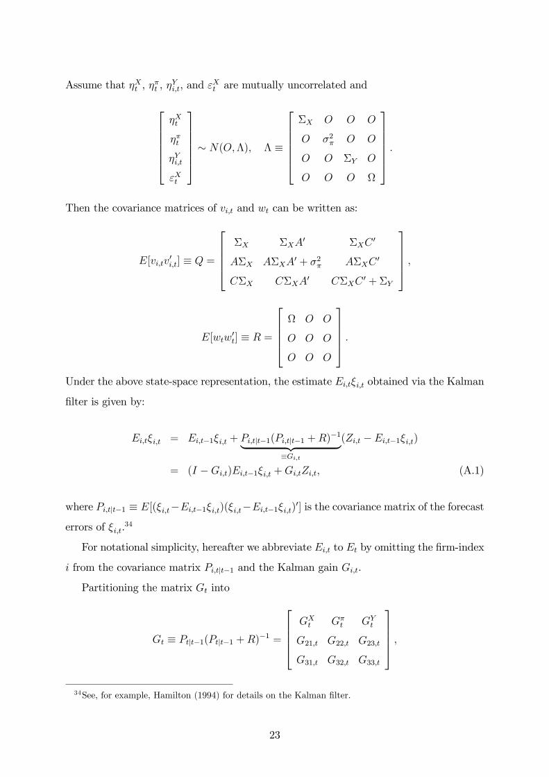
Assume that �Xt , ��t , �
Yi;t, and "
Xt are mutually uncorrelated and
2666664�Xt
��t
�Yi;t
"Xt
3777775 � N(O;�); � �
2666664�X O O O
O �2� O O
O O �Y O
O O O
3777775 :
Then the covariance matrices of vi;t and wt can be written as:
E[vi;tv0i;t] � Q =
26664�X �XA
0 �XC0
A�X A�XA0 + �2� A�XC
0
C�X C�XA0 C�XC
0 + �Y
37775 ;
E[wtw0t] � R =
26664 O O
O O O
O O O
37775 :Under the above state-space representation, the estimate Ei;t�i;t obtained via the Kalman
�lter is given by:
Ei;t�i;t = Ei;t�1�i;t + Pi;tjt�1(Pi;tjt�1 +R)�1| {z }
�Gi;t
(Zi;t � Ei;t�1�i;t)
= (I �Gi;t)Ei;t�1�i;t +Gi;tZi;t; (A.1)
where Pi;tjt�1 � E[(�i;t�Ei;t�1�i;t)(�i;t�Ei;t�1�i;t)0] is the covariance matrix of the forecast
errors of �i;t.34
For notational simplicity, hereafter we abbreviate Ei;t to Et by omitting the �rm-index
i from the covariance matrix Pi;tjt�1 and the Kalman gain Gi;t.
Partitioning the matrix Gt into
Gt � Ptjt�1(Ptjt�1 +R)�1 =
26664GXt G�t GYt
G21;t G22;t G23;t
G31;t G32;t G33;t
37775 ;
34See, for example, Hamilton (1994) for details on the Kalman �lter.
23
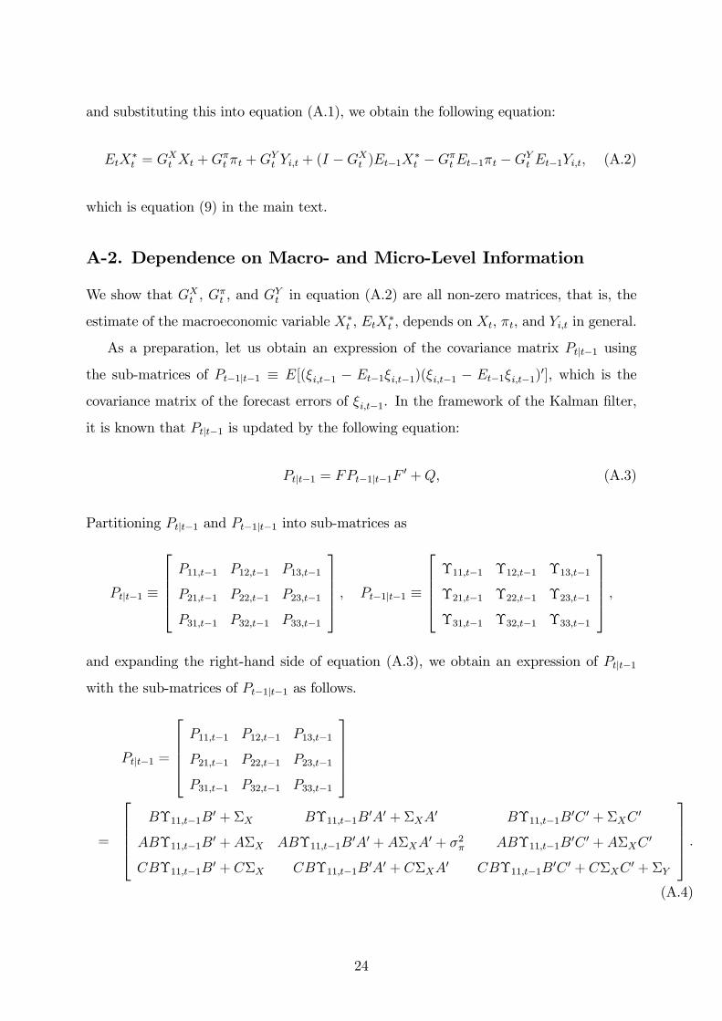
and substituting this into equation (A.1), we obtain the following equation:
EtX�t = G
Xt Xt +G
�t �t +G
Yt Yi;t + (I �GXt )Et�1X�
t �G�tEt�1�t �GYt Et�1Yi;t; (A.2)
which is equation (9) in the main text.
A-2. Dependence on Macro- and Micro-Level Information
We show that GXt , G�t , and G
Yt in equation (A.2) are all non-zero matrices, that is, the
estimate of the macroeconomic variable X�t , EtX
�t , depends on Xt, �t, and Yi;t in general.
As a preparation, let us obtain an expression of the covariance matrix Ptjt�1 using
the sub-matrices of Pt�1jt�1 � E[(�i;t�1 � Et�1�i;t�1)(�i;t�1 � Et�1�i;t�1)0], which is the
covariance matrix of the forecast errors of �i;t�1. In the framework of the Kalman �lter,
it is known that Ptjt�1 is updated by the following equation:
Ptjt�1 = FPt�1jt�1F0 +Q; (A.3)
Partitioning Ptjt�1 and Pt�1jt�1 into sub-matrices as
Ptjt�1 �
26664P11;t�1 P12;t�1 P13;t�1
P21;t�1 P22;t�1 P23;t�1
P31;t�1 P32;t�1 P33;t�1
37775 ; Pt�1jt�1 �
26664�11;t�1 �12;t�1 �13;t�1
�21;t�1 �22;t�1 �23;t�1
�31;t�1 �32;t�1 �33;t�1
37775 ;
and expanding the right-hand side of equation (A.3), we obtain an expression of Ptjt�1
with the sub-matrices of Pt�1jt�1 as follows.
Ptjt�1 =
26664P11;t�1 P12;t�1 P13;t�1
P21;t�1 P22;t�1 P23;t�1
P31;t�1 P32;t�1 P33;t�1
37775
=
26664B�11;t�1B
0 + �X B�11;t�1B0A0 + �XA
0 B�11;t�1B0C 0 + �XC
0
AB�11;t�1B0 + A�X AB�11;t�1B
0A0 + A�XA0 + �2� AB�11;t�1B
0C 0 + A�XC0
CB�11;t�1B0 + C�X CB�11;t�1B
0A0 + C�XA0 CB�11;t�1B
0C 0 + C�XC0 + �Y
37775 :(A.4)
24
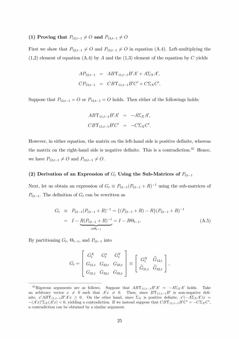
(1) Proving that P12;t�1 6= O and P13;t�1 6= O
First we show that P12;t�1 6= O and P13;t�1 6= O in equation (A.4). Left-multiplying the
(1,2) element of equation (A.4) by A and the (1,3) element of the equation by C yields
AP12;t�1 = AB�11;t�1B0A0 + A�XA
0;
CP13;t�1 = CB�11;t�1B0C 0 + C�XC
0:
Suppose that P12;t�1 = O or P13;t�1 = O holds. Then either of the followings holds:
AB�11;t�1B0A0 = �A�XA0;
CB�11;t�1B0C 0 = �C�XC 0:
However, in either equation, the matrix on the left-hand side is positive de�nite, whereas
the matrix on the right-hand side is negative de�nite. This is a contradiction.35 Hence,
we have P12;t�1 6= O and P13;t�1 6= O.
(2) Derivation of an Expression of Gt Using the Sub-Matrices of Ptjt�1
Next, let us obtain an expression of Gt � Ptjt�1(Ptjt�1 + R)�1 using the sub-matrices of
Ptjt�1. The de�nition of Gt can be rewritten as
Gt � Ptjt�1(Ptjt�1 +R)�1 = f(Ptjt�1 +R)�Rg(Ptjt�1 +R)�1
= I �R(Ptjt�1 +R)�1| {z }��t�1
= I �R�t�1: (A.5)
By partitioning Gt, �t�1, and Ptjt�1 into
Gt =
26664GXt G�t GYt
G21;t G22;t G23;t
G31;t G32;t G33;t
37775 �24 GXt
eG12;teG21;t eG22;t35 ;
35Rigorous arguments are as follows. Suppose that AB�11;t�1B0A0 = �A�XA0 holds. Takean arbitrary vector x 6= 0 such that A0x 6= 0. Then, since B�11;t�1B0 is non-negative de�-nite, x0AB�11;t�1B0A0x � 0. On the other hand, since �X is positive de�nite, x0(�A�XA0)x =�(A0x)0�X(A0x) < 0, yielding a contradiction. If we instead suppose that CB�11;t�1B0C 0 = �C�XC 0,a contradiction can be obtained by a similar argument.
25
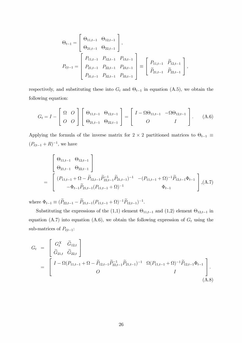
�t�1 =
24 �11;t�1 �12;t�1
�21;t�1 �22;t�1
35 ;
Ptjt�1 =
26664P11;t�1 P12;t�1 P13;t�1
P21;t�1 P22;t�1 P23;t�1
P31;t�1 P32;t�1 P33;t�1
37775 �24 P11;t�1 eP12;t�1eP21;t�1 eP22;t�1
35 ;
respectively, and substituting these into Gt and �t�1 in equation (A.5), we obtain the
following equation:
Gt = I �
24 O
O O
3524 �11;t�1 �12;t�1
�21;t�1 �22;t�1
35 =24 I � �11;t�1 ��12;t�1
O I
35 : (A.6)
Applying the formula of the inverse matrix for 2 � 2 partitioned matrices to �t�1 �
(Ptjt�1 +R)�1, we have
24 �11;t�1 �12;t�1
�21;t�1 �22;t�1
35=
24 (P11;t�1 + � eP12;t�1 eP�122;t�1 eP21;t�1)�1 �(P11;t�1 + )�1 eP12;t�1�t�1��t�1 eP21;t�1(P11;t�1 + )�1 �t�1
35 ;(A.7)where �t�1 � ( eP22;t�1 � eP21;t�1(P11;t�1 + )�1 eP12;t�1)�1.Substituting the expressions of the (1,1) element �11;t�1 and (1,2) element �12;t�1 in
equation (A.7) into equation (A.6), we obtain the following expression of Gt using the
sub-matrices of Ptjt�1:
Gt =
24 GXteG12;teG21;t eG22;t
35=
24 I � (P11;t�1 + � eP12;t�1 eP�122;t�1 eP21;t�1)�1 (P11;t�1 + )�1 eP12;t�1�t�1
O I
35 :(A.8)
26
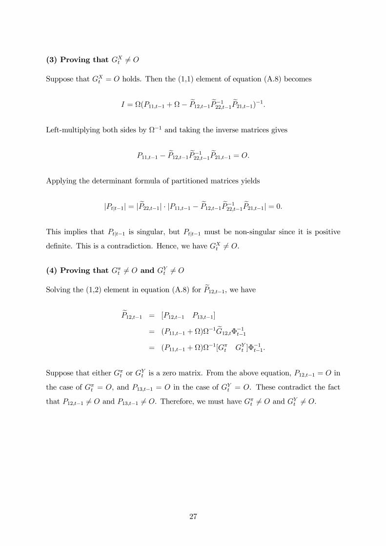
(3) Proving that GXt 6= O
Suppose that GXt = O holds. Then the (1,1) element of equation (A.8) becomes
I = (P11;t�1 + � eP12;t�1 eP�122;t�1 eP21;t�1)�1:Left-multiplying both sides by �1 and taking the inverse matrices gives
P11;t�1 � eP12;t�1 eP�122;t�1 eP21;t�1 = O:Applying the determinant formula of partitioned matrices yields
jPtjt�1j = j eP22;t�1j � jP11;t�1 � eP12;t�1 eP�122;t�1 eP21;t�1j = 0:This implies that Ptjt�1 is singular, but Ptjt�1 must be non-singular since it is positive
de�nite. This is a contradiction. Hence, we have GXt 6= O.
(4) Proving that G�t 6= O and GYt 6= O
Solving the (1,2) element in equation (A.8) for eP12;t�1, we haveeP12;t�1 = [P12;t�1 P13;t�1]
= (P11;t�1 + )�1 eG12;t��1t�1
= (P11;t�1 + )�1[G�t GYt ]�
�1t�1:
Suppose that either G�t or GYt is a zero matrix. From the above equation, P12;t�1 = O in
the case of G�t = O, and P13;t�1 = O in the case of GYt = O. These contradict the fact
that P12;t�1 6= O and P13;t�1 6= O. Therefore, we must have G�t 6= O and GYt 6= O.
27
References
[1] Andrews, D. W. K. and B. Lu (2001), "Consistent Model and Moment Selection
Procedures for GMM Estimation with Application to Dynamic Panel Data Models,"
Journal of Econometrics, 101, 123-164.
[2] Bank of Japan (2018), "Outlook for Economic Activity and Prices," July 2018.
[3] Blundell, R. and S. Bond (1998), "Initial Conditions and Moment Restrictions in
Dynamic Panel Data Models," Journal of Econometrics, 87, 115-143.
[4] Boneva, L., J. Cloyne, M. Weale, and T. Wieladek (2016), "Firms�Expectations and
Price-Setting: Evidence from Micro Data," Bank of England External MPC Unit
Discussion Paper, No. 48.
[5] Coibion, O. and Y. Gorodnichenko (2015), "Information Rigidity and the Expecta-
tions Formation Process: A Simple Framework and New Facts," American Economic
Review, 105(8), 2644-2678.
[6] � � � , � � � , and R. Kamdar (2018a), "The Formation of Expectations, In�ation,
and the Phillips Curve," Journal of Economic Literature, 56(4), 1447-1491.
[7] � � � , � � � , and S. Kumar (2018b), "How Do Firms Form Their Expectations?
New Survey Evidence," American Economic Review, 108(9), 2671-2713.
[8] Economic Analysis Group, Research and Statistics Department, the Bank of Japan
(2017), "Kigyo No Infure Yosou Keisei Ni Kansuru Shin Jijitsu: Part II �Kikai
Gakushu Approach � (New Facts about Firms� In�ation Expectations: Part II �
Machine Learning Approach �)", Bank of Japan Working Paper Series, No. 17-J-4.
(in Japanese)
[9] Evans, G. W. and S. Honkapohja (1999), "Learning Dynamics," in Handbook of
Macroeconomics: Volume 1A, edited by J. B. Taylor and M. Woodford, 449-542.
[10] � � � and � � � (2001), Learning and Expectations in Macroeconomics, Princeton
University Press.
28
[11] Gabaix, X. (2014), "A Sparsity-Based Model of Bounded Rationality," Quarterly
Journal of Economics, 129 (4), 1661-1710.
[12] Hamilton, J. D. (1994), Time Series Analysis, Princeton University Press.
[13] Inamura, K., K. Hiyama, and K. Shiotani (2017), "In�ation Outlook and Business
Conditions of Firms: Evidence from the Tankan Survey," IFC Bulletin, No. 43.
[14] Kaihatsu, S. and N. Shiraki (2016), "Firms�In�ation Expectations and Wage-Setting
Behaviors," Bank of Japan Working Paper Series, No. 16-E-10.
[15] Kitamura, T. and M. Tanaka (2019), "Firms�In�ation Expectations under Rational
Inattention and Sticky Information: An Analysis with a Small-Scale Macroeconomic
Model," Bank of Japan Working Paper Series, No. 19-E-16.
[16] Koga, M., K. Yoshino, and T. Sakata (2019), "Strategic Complementarity and Asym-
metric Price Setting among Firms," Bank of Japan Working Paper Series, No.19-E-5.
[17] Kumar, S., H. Afrouzi, O. Coibion, and Y. Gorodnichenko (2015), "In�ation Target-
ing Does Not Anchor In�ation Expectations: Evidence from Firms in New Zealand,"
Brookings Papers on Economic Activity, 2015(2), 151-225.
[18] Lucas, R. E. (1972), "Expectations and the Neutrality of Money," Journal of Eco-
nomic Theory, 4(2), 103-124.
[19] Mackowiak, B. and M. Wiederholt (2009), "Optimal Sticky Prices under Rational
Inattention," American Economic Review, 99(3), 769-803.
[20] Mankiw, G. N. and R. Reis (2002), "Sticky Price versus Sticky Information: A
Proposal to Replace the New Keynesian Phillips Curve," Quarterly Journal of Eco-
nomics, 117(4), 1295-1328.
[21] Maruyama, T. and K. Suganuma (2019), "In�ation Expectations Curve in Japan,"
Bank of Japan Working Paper Series, No. 19-E-6.
[22] Phelps, E. S. (1970), "Introduction: The New Microeconomics in Employment and
In�ation Theory," in Microeconomic Foundations of Employment and In�ation The-
ory, edited by E. S. Phelps et al.
29
[23] Reis, R. (2006), "Inattentive Producers," Review of Economic Studies, 73(3), 793-
821.
[24] Richards, S. and M. Verstraete (2016), "Understanding Firm�s In�ation Expecta-
tions Using the Bank of Canada�s Business Outlook Survey," Bank of Canada Sta¤
Working Paper, 2016-7.
[25] Sargent, T. J. (1993), Bounded Rationality in Macroeconomics, Oxford University
Press.
[26] Sims, C. A. (2003), "Implications of Rational Inattention," Journal of Monetary
Economics, 50(3): 665-690.
[27] Uno, Y., S. Naganuma, and N. Hara (2018), "New Facts about Firms� In�ation
Expectations: Simple Tests for a Sticky Information Model," Bank of Japan Working
Paper Series, No. 18-E-14.
[28] Woodford, M. (2003), "Imperfect Common Knowledge and the E¤ects of Monetary
Policy," in P. Aghion, R. Frydman, J. Stiglitz and M. Woodford, eds. Knowledge,
Information, and Expectations in Modern Macroeconomics: In Honor of Edmund S.
Phelps, Princeton University Press.
[29] Wooldridge, J. M. (2010), Econometric Analysis of Cross Section and Panel Data
2nd Edition, The MIT Press.
[30] Zbaracki, M. J., M. Ritson, D. Levy, S. Dutta, and M. Bergen (2004), "Managerial
and Customer Costs of Price Adjustment: Direct Evidence from Industrial Markets,"
Review of Economics and Statistics, 86(2), 514-533.
30
(1) OLS regression by firm size and industry
Note: ** and * indicate the 5% and 10% significance level, respectively.
Note: Standard errors are shown in parentheses (adjusted by Newey-West method for serial correlations).
(2) Panel-data regression
Notes: 1. *** indicates the 1% significance level.
Notes: 1. Standard error is shown in parentheses (adjusted by Newey-West method for serial correlations).
Notes: 2. To take into account possible correlations among error terms in the cross-sectional dimension,
Notes: 2. the General FGLS method is employed.
Table 1: Test of FIRE for 1-year-ahead inflation expectations
2.74 ***
(0.10)
Adj. R2 0.19
Obs. 117
0.73
Semi-aggregate panel data of
3 industries 3 sizes
Large Small
3.28 ** 4.28 ** 3.14 * 2.99 ** 3.17 ** 2.85 ** 3.16 *
(1.41) (1.93) (1.47) (1.27) (1.37) (1.16) (1.50)
Adj. R2 0.10 0.10 0.07 0.10 0.17 0.08 0.07
Obs. 13 13 13 13 13 13 13
0.77 0.81 0.76 0.75 0.76 0.74 0.76
All
By firm size By industry
Manufacturing
(Materials)
Manufacturing
(Processing)
Medium-sized Non-
manufacturing
Note: For Change in Input Prices , Change in Output Prices , and Change in Interest Rate on Loans ,
Note: judgments are based on the change in conditions from three months prior to the time of the survey.
Note: For the other items, judgments are based on the conditions at the time of the survey.
Table 2: Answers for judgment items and assigned values
+1 0 -1
Change in Input Prices Rise Unchanged Fall
Change in Output Prices Rise Unchanged Fall
Domestic Supply and Demand
Conditions for Products and ServicesExcess demand Almost balanced Excess supply
Employment ConditionsInsufficient
employmentAdequate
Excess
employment
Business Conditions Favorable Not so favorable Unfavorable
Production CapacityInsufficient
capacityAdequate
Excess
capacity
Financial Position Easy Not so tight Tight
Lending Attitude of Financial
InstitutionsAccommodative Not so severe Severe
Change in Interest Rate on Loans Fall Unchanged Rise
(1) 1-year-ahead inflation expectations
(2) 5-year-ahead inflation expectations
Notes: 1. *** , **, and * indicate the 1%, 5%, and 10% significance level, respectively. Standard errors are shown in
Notes: 1. parentheses.
Notes: 2. p -values are reported for the tests of serial correlations and overidentification.
Table 3: Results of dynamic panel-data regression
1-period lag 0.40 *** 0.45 *** 0.42 *** 0.41 ***
of inflation expectations (0.04) (0.08) (0.07) (0.05)
2-period lag 0.10 *** 0.14 ** 0.09 0.12 ***
of inflation expectations (0.03) (0.07) (0.06) (0.05)
Input prices 0.04 *** 0.02 0.02 0.06 ***
(0.01) (0.02) (0.02) (0.02)
Output prices 0.03 ** 0.03 0.01 0.04 **
(0.01) (0.02) (0.02) (0.02)
Domestic demand 0.05 *** 0.00 0.03 0.05 ***
(0.01) (0.03) (0.02) (0.02)
Employment conditions 0.01 0.03 0.03 * -0.00
(0.01) (0.03) (0.02) (0.01)
Obs. 221,563 38,602 61,705 121,256
Number of firms 9,830 1,922 2,751 5,157
Test of serial correlations 0.48 0.73 0.63 0.42
Test of overidentification 0.25 0.33 0.27 0.37
All sizes Large Medium-sized Small
1-period lag 0.36 *** 0.56 *** 0.27 0.30 ***
of inflation expectations (0.07) (0.13) (0.23) (0.09)
2-period lag 0.09 0.24 ** -0.01 0.05
of inflation expectations (0.07) (0.12) (0.22) (0.09)
Input prices 0.03 -0.06 0.08 ** 0.02
(0.02) (0.04) (0.04) (0.03)
Output prices 0.03 0.03 0.02 0.05
(0.02) (0.04) (0.04) (0.03)
Domestic demand 0.01 -0.06 -0.01 0.03
(0.02) (0.04) (0.04) (0.02)
Employment conditions 0.01 -0.00 0.02 0.01
(0.02) (0.05) (0.03) (0.02)
Obs. 144,517 20,826 40,375 83,316
Number of firms 9,830 1,922 2,751 5,157
Test of serial correlations 0.77 0.18 0.73 0.84
Test of overidentification 0.84 0.73 0.12 0.42
Medium-sized SmallAll sizes Large
Notes: 1. *** and ** indicate the 1% and 5% significance level, respectively. Standard errors are shown in parentheses.
Notes: 2. p -values are reported for the tests of serial correlations and overidentification.
Notes: 3. The sample includes all firms. The column (1) in the table reproduces the results of the baseline case in
Notes: 3. Table 3.
Table 4: Results of panel-data regression with additional judgment items
(1) (2) (1) (2)
1-period lag 0.40 *** 0.41 *** 0.36 *** 0.33 ***
of inflation expectations (0.04) (0.04) (0.07) (0.09)
2-period lag 0.10 *** 0.12 *** 0.09 0.06
of inflation expectations (0.03) (0.04) (0.07) (0.08)
Input prices 0.04 *** 0.04 *** 0.03 0.02
(0.01) (0.01) (0.02) (0.02)
Output prices 0.03 ** 0.05 *** 0.03 0.07 ***
(0.01) (0.02) (0.02) (0.02)
Domestic demand 0.05 *** 0.05 *** 0.01 0.01
(0.01) (0.01) (0.02) (0.02)
Employment conditions 0.01 0.02 0.01 0.00
(0.01) (0.01) (0.02) (0.02)
Business conditions 0.01 0.00
(0.01) (0.01)
Production capacity -0.01 0.01
(0.02) (0.02)
Financial position -0.01 0.02
(0.01) (0.02)
Lending attitude 0.00 0.01
(0.01) (0.02)
Interest rate on loans -0.01 -0.02
(0.01) (0.02)
Obs. 221,563 201,188 144,517 132,415
Number of firms 9,830 9,830 9,830 9,830
Test of serial correlations 0.48 0.34 0.77 0.48
Test of overidentification 0.25 0.11 0.84 0.25
1-year-ahead inflation expectations 5-year-ahead inflation expectations
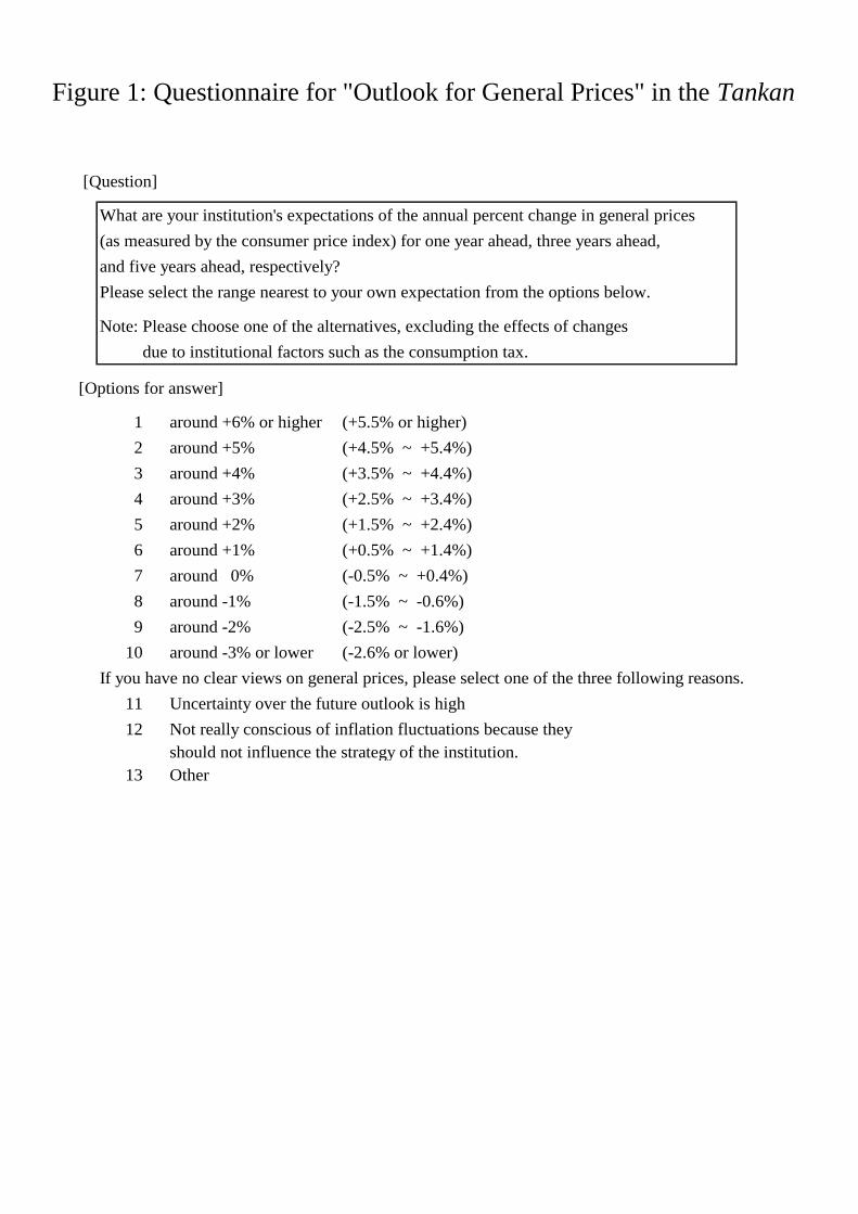
Figure 1: Questionnaire for "Outlook for General Prices" in the Tankan
[Question]
What are your institution's expectations of the annual percent change in general prices
(as measured by the consumer price index) for one year ahead, three years ahead,
and five years ahead, respectively?
Please select the range nearest to your own expectation from the options below.
Note: Please choose one of the alternatives, excluding the effects of changes
Note: due to institutional factors such as the consumption tax.
[Options for answer]
1 around +6% or higher (+5.5% or higher)
2 around +5% (+4.5% ~ +5.4%)
3 around +4% (+3.5% ~ +4.4%)
4 around +3% (+2.5% ~ +3.4%)
5 around +2% (+1.5% ~ +2.4%)
6 around +1% (+0.5% ~ +1.4%)
7 around 0% (-0.5% ~ +0.4%)
8 around -1% (-1.5% ~ -0.6%)
9 around -2% (-2.5% ~ -1.6%)
10 around -3% or lower (-2.6% or lower)
If you have no clear views on general prices, please select one of the three following reasons.
11 Uncertainty over the future outlook is high
12 Not really conscious of inflation fluctuations because they
should not influence the strategy of the institution.
13 Other
(1) Large revisions
(i) 1-year-ahead inflation expectations (ii) 5-year-ahead inflation expectations
Note: The graphs show percentage share of the number of respondents revising expectations by more than 2% points
Note: upward or downward, among all firms choosing numeric options.
(2) Irregular revisions
(i) 1-year-ahead inflation expectations (ii) 5-year-ahead inflation expectations
Note: The graphs show percentage share of the number of respondents revising expectations in the opposite direction
Note: to the previous survey, among all firms choosing numeric options.
Figure 2: Stability of the firms' answers for inflation expectations
0
5
10
15
20
25
30
14 15 16 17 18 19
Large firms
Medium-sized firms
Small firms
(%)
CY 0
5
10
15
20
25
30
14 15 16 17 18 19
(%)
CY
0
5
10
15
20
25
30
14 15 16 17 18 19
Large firms
Medium-sized firms
Small firms
(%)
CY 0
5
10
15
20
25
30
14 15 16 17 18 19
(%)
CY
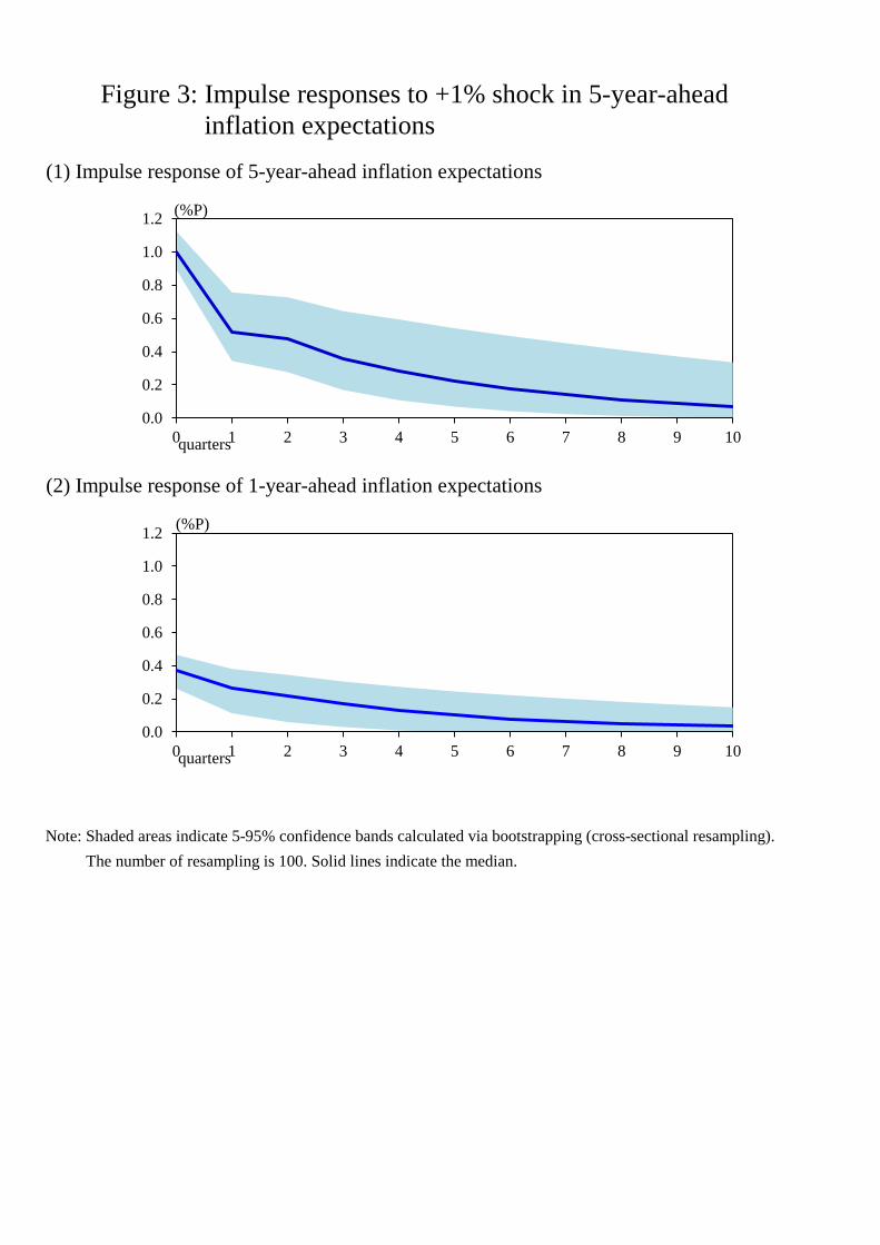
(1) Impulse response of 5-year-ahead inflation expectations
(2) Impulse response of 1-year-ahead inflation expectations
Note: Shaded areas indicate 5-95% confidence bands calculated via bootstrapping (cross-sectional resampling).
Note: The number of resampling is 100. Solid lines indicate the median.
Figure 3: Impulse responses to +1% shock in 5-year-ahead
Chainflation expectations
0.0
0.2
0.4
0.6
0.8
1.0
1.2
0 1 2 3 4 5 6 7 8 9 10quarters
(%P)
0.0
0.2
0.4
0.6
0.8
1.0
1.2
0 1 2 3 4 5 6 7 8 9 10quarters
(%P)
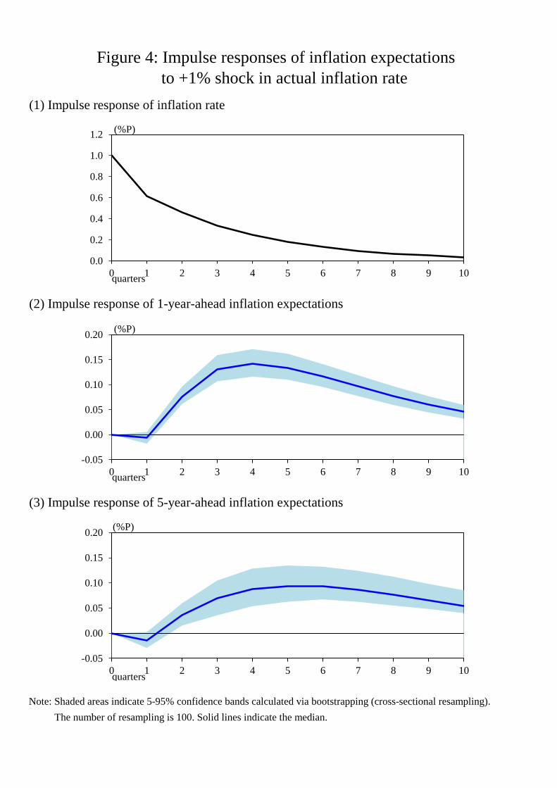
(1) Impulse response of inflation rate
(2) Impulse response of 1-year-ahead inflation expectations
(3) Impulse response of 5-year-ahead inflation expectations
Note: Shaded areas indicate 5-95% confidence bands calculated via bootstrapping (cross-sectional resampling).
Note: The number of resampling is 100. Solid lines indicate the median.
Figure 4: Impulse responses of inflation expectations
to +1% shock in actual inflation rate
0.0
0.2
0.4
0.6
0.8
1.0
1.2
0 1 2 3 4 5 6 7 8 9 10
(%P)
quarters
-0.05
0.00
0.05
0.10
0.15
0.20
0 1 2 3 4 5 6 7 8 9 10
(%P)
quarters
-0.05
0.00
0.05
0.10
0.15
0.20
0 1 2 3 4 5 6 7 8 9 10
(%P)
quarters
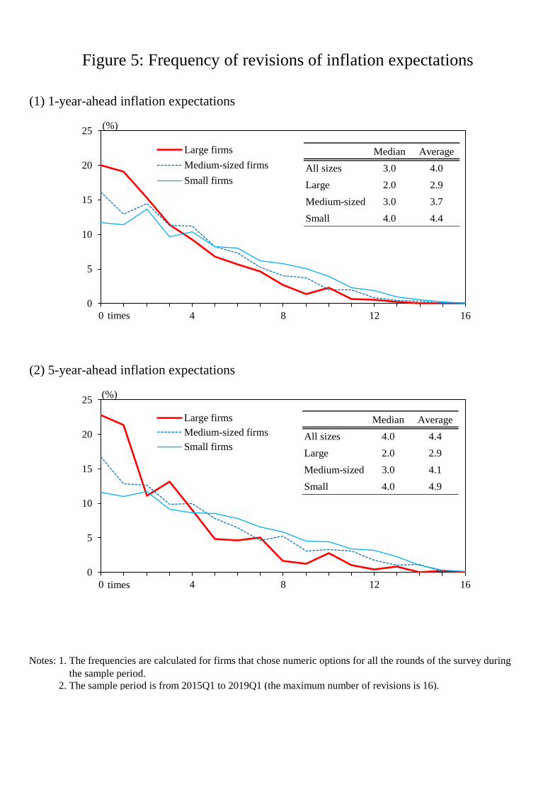
(1) 1-year-ahead inflation expectations
(2) 5-year-ahead inflation expectations
Notes: 1. The frequencies are calculated for firms that chose numeric options for all the rounds of the survey during
Notes: 1. the sample period.
Notes: 2. The sample period is from 2015Q1 to 2019Q1 (the maximum number of revisions is 16).
Figure 5: Frequency of revisions of inflation expectations
0
5
10
15
20
25
0 4 8 12 16
Large firms
Medium-sized firms
Small firms
(%)
times
0
5
10
15
20
25
0 4 8 12 16
Large firms
Medium-sized firms
Small firms
(%)
times
Median Average
All sizes 3.0 4.0
Large 2.0 2.9
Medium-sized 3.0 3.7
Small 4.0 4.4
Median Average
All sizes 4.0 4.4
Large 2.0 2.9
Medium-sized 3.0 4.1
Small 4.0 4.9