Embed Size (px)
Citation preview

The Hamiltonian structure of the nonlinearSchrödinger equation and the asymptotic
stability of its ground states
S. Cuccagna
Università di Trieste
Bertinoro 29 September 2011
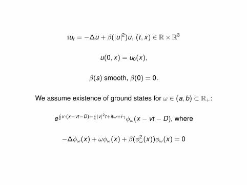
iut = −∆u + β(|u|2)u, (t , x) ∈ R× R3
u(0, x) = u0(x),
β(s) smooth, β(0) = 0.
We assume existence of ground states for ω ∈ (a,b) ⊂ R+:
ei2 v ·(x−vt−D)+ i
4 |v |2t+itω+iγϕω(x − vt − D), where
−∆ϕω(x) + ωϕω(x) + β(ϕ2ω(x))ϕω(x) = 0
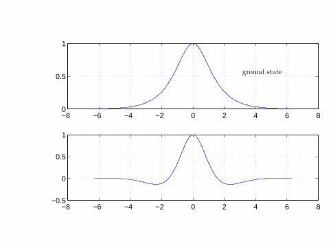
−8 −6 −4 −2 0 2 4 6 80
0.5
1
−8 −6 −4 −2 0 2 4 6 8−0.5
0
0.5
1
ground state
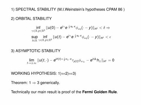
1) SPECTRAL STABILITY (M.I.Weinstein’s hypotheses CPAM 86 )
2) ORBITAL STABILITY
infγ∈R,y∈R3
∥u(0)− eiγei2 v0·xϕω0(· − y)∥H1 < δ ⇒
supt∈R
infγ∈R,y∈R3
∥u(t)− eiγei2 v0·xϕω0(· − y)∥H1 < ϵ
3) ASYMPTOTIC STABILITY
limt→±∞
∥u(t , ·)− eiθ(t)+ i2 v±·xτy(t)ϕω± − eit∆h±∥H1 = 0
WORKING HYPOTHESIS: 1)⇔2)⇔3)
Theorem: 1 ⇒ 3 generically.
Technically our main result is proof of the Fermi Golden Rule.
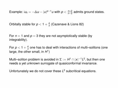
Example: iut = −∆u − |u|p−1u with p < n+2n−2 admits ground states.
Orbitally stable for p < 1 + 4n (Cazenave & Lions 82)
For n = 1 and p = 3 they are not asymptotically stable (byintegrability).
For p < 1 + 4n one has to deal with interactions of multi–solitons (one
large, the other small, in H1)
Multi–soliton problem is avoided in Σ := H1 ∩ |x |−1L2, but then oneneeds a yet unknown surrogate of quasiconformal invariance.
Unfortunately we do not cover these L2 subcritical equations.
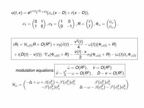
u(t , x) = ei( v·(x−D)2 +ϑ)(ϕω(x − D) + r(x − D)),
σ1 =
(0 11 0
), σ3 =
(1 00 −1
),R =
(rr
),Φω =
(ϕω
ϕω
).
iRt = Hω(t)R + O(R2) + σ3(ϑ(t)−v2(t)
4− ω(t))(Φω(t) + R)
+ i(D(t)− v(t)) · ∇x (Φω(t) + R)− v(t) · x2
σ3(Φω(t) + R)− iω(t)∂ωΦω(t)
modulation equations:ω = O(R2) , v = O(R2)
ϑ− v2
4 − ω = O(R2) , D − v = O(R2)
Hω =
(−∆+ ω + β(ϕ2
ω) + β′(ϕ2ω)ϕ
2ω β′(ϕ2
ω)ϕ2ω
−β′(ϕ2ω)ϕ
2ω ∆− ω − β(ϕ2
ω)− β′(ϕ2ω)ϕ
2ω
)
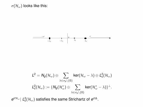
σ(Hω) looks like this:
0
λ2λ1
−λ1−λ2
ω−ω
L2 = Ng(Hω)⊕∑
λ∈σp\0
ker(Hω − λ)⊕ L2c(Hω)
L2c(Hω) := Ng(H∗
ω)⊕∑
λ∈σp\0
ker(H∗ω − λ)⊥.
eitHω | L2c(Hω) satisfies the same Strichartz of eit∆.
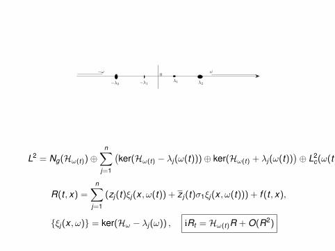
0
λ2λ1
−λ1−λ2
ω−ω
L2 = Ng(Hω(t))⊕n∑
j=1
(ker(Hω(t) − λj(ω(t)))⊕ ker(Hω(t) + λj(ω(t))
)⊕ L2
c(ω(t))
R(t , x) =n∑
j=1
(zj(t)ξj(x , ω(t)) + z j(t)σ1ξj(x , ω(t))) + f (t , x),
ξj(x , ω) = ker(Hω − λj(ω)) , iRt = Hω(t)R + O(R2)
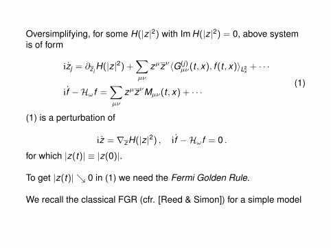
Oversimplifying, for some H(|z|2) with Im H(|z|2) = 0, above systemis of form
izj = ∂z jH(|z|2) +
∑µν
zµzν⟨G(j)µν(t , x), f (t , x)⟩L2
x+ · · ·
if −Hωf =∑µν
zµzνMµν(t , x) + · · ·(1)
(1) is a perturbation of
iz = ∇zH(|z|2) , if −Hωf = 0 .
for which |z(t)| ≡ |z(0)|.
To get |z(t)| 0 in (1) we need the Fermi Golden Rule.
We recall the classical FGR (cfr. [Reed & Simon]) for a simple model
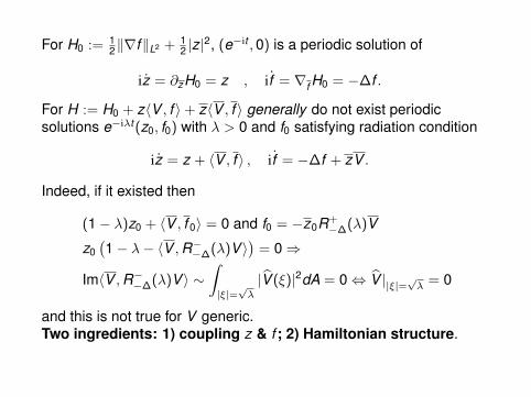
For H0 := 12∥∇f∥L2 + 1
2 |z|2, (e−it ,0) is a periodic solution of
iz = ∂zH0 = z , if = ∇f H0 = −∆f .
For H := H0 + z⟨V , f ⟩+ z⟨V , f ⟩ generally do not exist periodicsolutions e−iλt(z0, f0) with λ > 0 and f0 satisfying radiation condition
iz = z + ⟨V , f ⟩ , if = −∆f + zV .
Indeed, if it existed then
(1 − λ)z0 + ⟨V , f 0⟩ = 0 and f0 = −z0R+−∆(λ)V
z0(1 − λ− ⟨V ,R−
−∆(λ)V ⟩)= 0 ⇒
Im⟨V ,R−−∆(λ)V ⟩ ∼
∫|ξ|=
√λ
|V (ξ)|2dA = 0 ⇔ V ||ξ|=√λ = 0
and this is not true for V generic.Two ingredients: 1) coupling z & f ; 2) Hamiltonian structure.
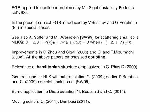
FGR applied in nonlinear problems by M.I.Sigal (Instability Periodicsol’s 93).
In the present context FGR introduced by V.Buslaev and G.Perelman(95) in special cases.
See also A. Soffer and M.I.Weinstein [SW99] for scattering small sol’sNLKG: u −∆u + V (x)u + m2u + β(u) = 0 when σd (−∆+ V ) = ∅.
Improvements in G.Zhou and Sigal (2006) and C. and T.Mizumachi(2008). All the above papers emphasized coupling.
Relevance of hamiltonian structure emphasized in C. Phys.D (2009)
General case for NLS without translation C. (2009); earlier D.Bambusiand C. (2009) complete solution of [SW99].
Some application to Dirac equation N. Boussaid and C. (2011).
Moving soliton: C. (2011), Bambusi (2011).
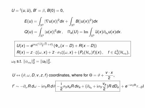
U = t(u,u), B′ = β, B(0) = 0,
E(u) =∫R3
|∇u(x)|2dx +
∫R3
B(|u(x)|2)dx
Q(u) =∫R3
|u(x)|2dx , Πa(U) = Im∫R3
u(x)∂xau(x)dx .
U(x) = eiσ3(v·(x−D)
2 +ϑ) (Φω(x − D) + R(x − D))
R(x) = z · ξ(ω, x) + z · σ1ξ(ω, x) + (Pc(Hω)f )(x) , f ∈ L2c(Hω0),
ω0 s.t. ∥ϕω0∥22 = ∥u0∥2
2.
U ↔ (ϑ, ω,D, v , z, f ) coordinates, where for Θ = ϑ+v · x
2,
f ′ ∼ −∂ωR dω − iσ3R dϑ − i2σ3xaR dva + (∂xa + iσ3
va
2)R dDa + e−iσ3Θτ−DI
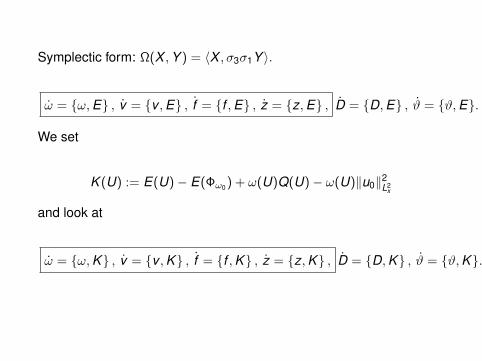
Symplectic form: Ω(X ,Y ) = ⟨X , σ3σ1Y ⟩.
ω = ω,E , v = v ,E , f = f ,E , z = z,E , D = D,E , ϑ = ϑ,E.
We set
K (U) := E(U)− E(Φω0) + ω(U)Q(U)− ω(U)∥u0∥2L2
x
and look at
ω = ω,K , v = v ,K , f = f ,K , z = z,K , D = D,K , ϑ = ϑ,K.
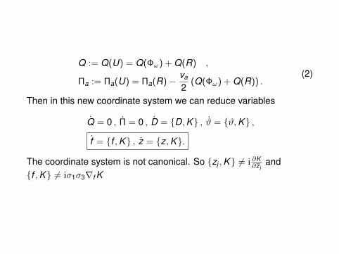
Q := Q(U) = Q(Φω) + Q(R) ,
Πa := Πa(U) = Πa(R)− va
2(Q(Φω) + Q(R)) .
(2)
Then in this new coordinate system we can reduce variables
Q = 0 , Π = 0 , D = D,K , ϑ = ϑ,K ,
f = f ,K , z = z,K.
The coordinate system is not canonical. So zj ,K = i ∂K∂z j
andf ,K = iσ1σ3∇f K
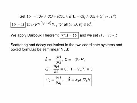
Set Ω0 := idϑ ∧ dQ + idDa ∧ dΠa + dzj ∧ dz j + ⟨f ′|σ3σ1f ′⟩.
Ω0 = Ω at τDeiσ3( v·x2 +ϑ)Φω0 for all (ϑ,D, v) ∈ R7.
We apply Darboux Theorem: F∗Ω = Ω0 and we set H := K F
Scattering and decay equivalent in the two coordinate systems andboxed formulas be semilinear NLS:
ϑ = −∂H∂Q
, D = −∇ΠH ,
Q =∂H∂ϑ
≡ 0 , Π = ∇DH ≡ 0
izj =∂H∂z j
, if = σ3σ1∇f H .
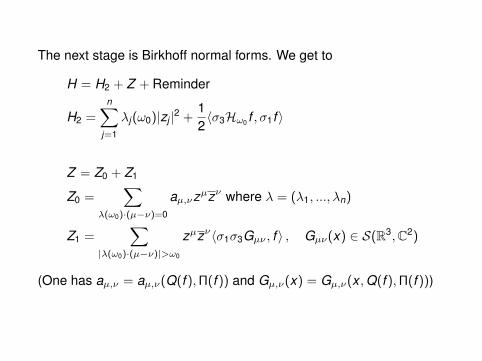
The next stage is Birkhoff normal forms. We get to
H = H2 + Z + Reminder
H2 =n∑
j=1
λj(ω0)|zj |2 +12⟨σ3Hω0 f , σ1f ⟩
Z = Z0 + Z1
Z0 =∑
λ(ω0)·(µ−ν)=0
aµ,νzµzν where λ = (λ1, ..., λn)
Z1 =∑
|λ(ω0)·(µ−ν)|>ω0
zµzν⟨σ1σ3Gµν , f ⟩ , Gµν(x) ∈ S(R3,C2)
(One has aµ,ν = aµ,ν(Q(f ),Π(f )) and Gµ,ν(x) = Gµ,ν(x ,Q(f ),Π(f )))
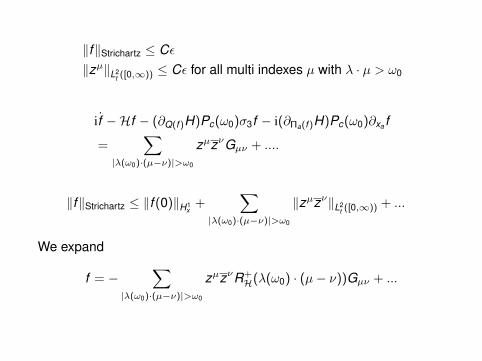
∥f∥Strichartz ≤ Cϵ
∥zµ∥L2t ([0,∞)) ≤ Cϵ for all multi indexes µ with λ · µ > ω0
if −Hf − (∂Q(f )H)Pc(ω0)σ3f − i(∂Πa(f )H)Pc(ω0)∂xa f
=∑
|λ(ω0)·(µ−ν)|>ω0
zµzνGµν + ....
∥f∥Strichartz ≤ ∥f (0)∥H1x+
∑|λ(ω0)·(µ−ν)|>ω0
∥zµzν∥L2t ([0,∞)) + ...
We expand
f = −∑
|λ(ω0)·(µ−ν)|>ω0
zµzνR+H(λ(ω0) · (µ− ν))Gµν + ...
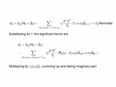
izj = ∂z j(H2 + Z0) +
∑|λ(ω0)·(µ′−ν′)|>ω0
νjzµ′
zν′
z j⟨f , σ1σ3Gµ′ν′⟩+ ∂z j
Reminder.
Substituting for f , the significant terms are
izj = ∂z j(H2 + Z0)
−∑
λ(ω0)·µ=λ(ω0)·ν′>ω0
ν′jzµzν′
z j⟨R+
H(µ · λ(ω0))Gµ0, σ1σ3G0ν′⟩.
Multiplying by λj(ω0)z j , summing up and taking imaginary part
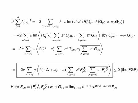
∂t
n∑j=1
λj |zj |2 = −2∑
λ·µ=λ·ν>ω0
λ · ν Im(zµzν⟨R+
H(µ · λ)Gµ0, σ1σ3G0ν⟩)
= −2∑κ>ω0
κ Im
⟨R+
H(κ)∑
λ·µ=κ
zµGµ0, σ3
∑λ·µ=κ
zµGµ0
⟩(by Gµν = −σ1Gνµ)
= −2π∑κ>ω0
κ
⟨δ (H− κ)
∑λ·µ=κ
zµGµ0, σ3
∑λ·µ=κ
zµGµ0
⟩
= −2π∑κ>ω0
κ
⟨δ(−∆+ ω0 − κ)
∑λ·µ=κ
zµF (1)µ0 ,
∑λ·µ=κ
zµF (1)µ0
⟩≤ 0 (the FGR)
Here Fµ0 = (F (1)µ0 ,F
(2)µ0 ) with Gµ0 = limt∞ e−itHωeitσ3(−∆+ω)Fµ0
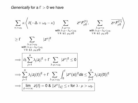
Generically for a Γ > 0 we have
∑κ>ω0
κ
⟨δ(−∆+ ω0 − κ)
∑λ·µ=κ
with λ·µ−λk<ω0∀ k s.t. µk =0
zµF (1)µ0 ,
∑λ·µ=κ
with λ·µ−λk<ω0∀ k s.t. µk =0
zµF (1)µ0
⟩
≥ Γ∑
λ·µ>ω0with λ·µ−λk<ω0∀ k s.t. µk =0
|zµ|2
=⇒ ∂t
n∑j=1
λj |zj |2 + Γ∑
λ·µ>ω0
|zµ|2 ≤ 0
=⇒n∑
j=1
λj |zj(t)|2 + Γ∑
λ·µ>ω0
∫ t
0|zµ(s)|2ds ≤
n∑j=1
λj |zj(0)|2
=⇒ limz→+∞
z(t) = 0 & ∥zµ∥L2t≤ ϵ for λ · µ > ω0.
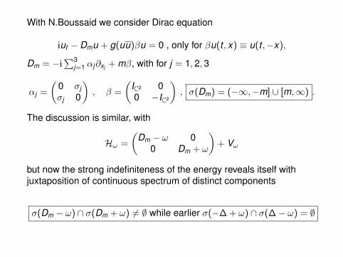
With N.Boussaid we consider Dirac equation
iut − Dmu + g(uu)βu = 0 , only for βu(t , x) ≡ u(t ,−x),
Dm = −i∑3
j=1 αj∂xj + mβ, with for j = 1,2,3
αj =
(0 σjσj 0
), β =
(IC2 00 −IC2
), σ(Dm) = (−∞,−m] ∪ [m,∞) .
The discussion is similar, with
Hω =
(Dm − ω 0
0 Dm + ω
)+ Vω
but now the strong indefiniteness of the energy reveals itself withjuxtaposition of continuous spectrum of distinct components
σ(Dm − ω) ∩ σ(Dm + ω) = ∅ while earlier σ(−∆+ ω) ∩ σ(∆− ω) = ∅
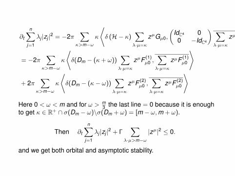
∂t
n∑j=1
λj |zj |2 = −2π∑
κ>m−ω
κ
⟨δ (H− κ)
∑λ·µ=κ
zµGµ0,
(IdC4 0
0 −IdC4
) ∑λ·µ=κ
zµGµ0
⟩
= −2π∑
κ>m−ω
κ
⟨δ(Dm − (κ+ ω))
∑λ·µ=κ
zµF (1)µ0 ,
∑λ·µ=κ
zµF (1)µ0
⟩
+ 2π∑
κ>m−ω
κ
⟨δ(Dm − (κ− ω))
∑λ·µ=κ
zµF (2)µ0 ,
∑λ·µ=κ
zµF (2)µ0
⟩
Here 0 < ω < m and for ω > m3 the last line = 0 because it is enough
to get κ ∈ R+ ∩ σ(Dm − ω)\σ(Dm + ω) = [m − ω,m + ω).
Then ∂t
n∑j=1
λj |zj |2 + Γ∑
λ·µ>m−ω
|zµ|2 ≤ 0.
and we get both orbital and asymptotic stability.