UPTEC F 18064

Examensarbete 30 hpDecember 2018

The Impact of Antennas on Radiolink Performance in Frequency Hopping Scenarios

Sofia Bergström

Teknisk- naturvetenskaplig fakultet UTH-enheten Besöksadress: Ångströmlaboratoriet Lägerhyddsvägen 1 Hus 4, Plan 0 Postadress: Box 536 751 21 Uppsala Telefon: 018 – 471 30 03 Telefax: 018 – 471 30 00 Hemsida: http://www.teknat.uu.se/student

Abstract

The Impact of Antennas on Radiolink Performance inFrequency Hopping Scenarios

Sofia Bergström

This paper investigates how the communication performance of frequency hoppingsystems are affected by the antenna parameters. The data are generated fromAntenna Toolbox in Matlab for the case of two dipole antennas is free space.Non-orthogonal and orthogonal frequency hopping are used and the statistical impactfrom the antenna on the SINR is investigated. The results can be used to see the wavepropagation margin and also see the effects of out-of-bands emissions in frequencyhopping systems.

The numerical generated model is compared to two isotropic antenna models and itshows that the isotropic models are relatively good despite its simplicity in this case.It does however not capture the spread caused by the directivity. Another model iscreated which mimic the numerical generated statistical distribution. This model usesthe theoretical probability of a collision for both orthogonal and non-orthogonalfrequency hopping. The model also uses mean values of directivity, s-parameters andthe spread of the gain to calculate a statistical antenna model. This model is betterthan the isotropic for the tested cases and shows that it is possible to generate astatistical model.

ISSN: 1401-5757, UPTEC F 18064Examinator: Tomas NybergÄmnesgranskare: Mikael SternadHandledare: Tore Lindgren

Popularvetenskaplig sammanfattning

Inom detta examensarbete har antennens egenskaper och dess inverkan pa kommunikationssyste-met undersoks for frekvenshoppande system som en del av KORINT-projektet pa Totalforsvaretsforskningsinstitut, FOI. En antennmodell som tar hansyn till antennforstarkning, impedans-matchning och kopplingen mellan antenner ar implementerad i Matlab. Varden pa isolation,intern reflektion och direktivitet ar generade med Antenna Toolbox i Matlab for ett fall dar tvadipolantenner ar placerade i fri rymd. Olika scenarios relaterade till frekvenshop ar testade ochden statistiska fordelningen av SINR ar undersokt.

Modellen ar jamford med tva vanligt forekommande isotropa modeller och det visade sig attbada isotropa modellerna ar relativt bra trots grova forenklingar. Vad modellerna inte gor aratt fanga spridningen orsakat av antennforstarkningen eller forandringen da avstandet mellanantennerna andras vilket kan resultera i felberaknad overforingsformaga. En ytterligare modellhar skapas med mal att imitera den Matlabgenererade modellen vilket den lyckas gora bara formedelvardet pa s-parametrar, direktivitet och for spridningen pa antennforstarkningen. Model-len visar att det inte kravs mycket information for att skapa en godtycklig modell. Modellen harocksa fordelen att den inte behover anvanda Antennpaketet fran Matlab eller nagra upprepadeMonte Carlo loopar. Modellen anvander teoretiskt beraknande sannolikheter for kollisionsriskenmed sidband och det visar sig vara relativt bra pa att prediktera sannolikhetsfordelningen. Allamodeller i denna rapport ar grovt forenklade men kan anda anvandas for att ge en forsta inblicki hur antennen paverkar ett frekvenshoppande kommunikationssystem.

Contents

1 Introduction 11.1 Background . . . . . . . . . . . . . . . . . . . . . . . . . . . . . . . . . . . . . . . 11.2 Thesis objective . . . . . . . . . . . . . . . . . . . . . . . . . . . . . . . . . . . . . 11.3 Scenarios . . . . . . . . . . . . . . . . . . . . . . . . . . . . . . . . . . . . . . . . 2

1.3.1 Delimitations . . . . . . . . . . . . . . . . . . . . . . . . . . . . . . . . . . 21.4 Related work . . . . . . . . . . . . . . . . . . . . . . . . . . . . . . . . . . . . . . 21.5 Outline of the thesis . . . . . . . . . . . . . . . . . . . . . . . . . . . . . . . . . . 3

2 Theory 42.1 The communication system . . . . . . . . . . . . . . . . . . . . . . . . . . . . . . 42.2 Antennas . . . . . . . . . . . . . . . . . . . . . . . . . . . . . . . . . . . . . . . . 5

2.2.1 Directivity and gain . . . . . . . . . . . . . . . . . . . . . . . . . . . . . . 52.2.2 The antenna as an electrical component . . . . . . . . . . . . . . . . . . . 52.2.3 Impedance matching . . . . . . . . . . . . . . . . . . . . . . . . . . . . . . 7

2.3 Signal, noise and interference . . . . . . . . . . . . . . . . . . . . . . . . . . . . . 92.4 Frequency hopping system . . . . . . . . . . . . . . . . . . . . . . . . . . . . . . . 10

3 Antenna setup 113.1 Preprocessing . . . . . . . . . . . . . . . . . . . . . . . . . . . . . . . . . . . . . . 11

3.1.1 Generate data . . . . . . . . . . . . . . . . . . . . . . . . . . . . . . . . . 113.1.2 Impedance matching . . . . . . . . . . . . . . . . . . . . . . . . . . . . . . 12

3.2 Dependence of distance . . . . . . . . . . . . . . . . . . . . . . . . . . . . . . . . 123.2.1 s-parameters . . . . . . . . . . . . . . . . . . . . . . . . . . . . . . . . . . 133.2.2 Directivity . . . . . . . . . . . . . . . . . . . . . . . . . . . . . . . . . . . 133.2.3 Data for statistic model . . . . . . . . . . . . . . . . . . . . . . . . . . . . 14

4 The model 174.1 Simulation setup . . . . . . . . . . . . . . . . . . . . . . . . . . . . . . . . . . . . 174.2 Antenna models . . . . . . . . . . . . . . . . . . . . . . . . . . . . . . . . . . . . 18

4.2.1 Matlab model . . . . . . . . . . . . . . . . . . . . . . . . . . . . . . . . . . 184.2.2 Previously used models - isotropic . . . . . . . . . . . . . . . . . . . . . . 184.2.3 Statistic model . . . . . . . . . . . . . . . . . . . . . . . . . . . . . . . . . 18

5 Comparison of models 195.1 Overview . . . . . . . . . . . . . . . . . . . . . . . . . . . . . . . . . . . . . . . . 195.2 Probability comparisons . . . . . . . . . . . . . . . . . . . . . . . . . . . . . . . . 205.3 Dependence of distance . . . . . . . . . . . . . . . . . . . . . . . . . . . . . . . . 22

6 Discussion 246.1 Discussion of models . . . . . . . . . . . . . . . . . . . . . . . . . . . . . . . . . . 24

6.1.1 Matlab model . . . . . . . . . . . . . . . . . . . . . . . . . . . . . . . . . . 246.1.2 Isotropic model . . . . . . . . . . . . . . . . . . . . . . . . . . . . . . . . . 256.1.3 Statistical model . . . . . . . . . . . . . . . . . . . . . . . . . . . . . . . . 25

6.2 Discussion of method . . . . . . . . . . . . . . . . . . . . . . . . . . . . . . . . . . 266.3 Future work . . . . . . . . . . . . . . . . . . . . . . . . . . . . . . . . . . . . . . . 26

7 Conclusion 27

A Motivation of collision probabilities 29A.1 Probability for direct hit . . . . . . . . . . . . . . . . . . . . . . . . . . . . . . . . 29A.2 Probability for collision with a sideband in non-orthogonal frequency hopping

systems . . . . . . . . . . . . . . . . . . . . . . . . . . . . . . . . . . . . . . . . . 29A.3 Probability for collision with a sideband in orthogonal frequency hopping systems 30

Chapter 1

Introduction

1.1 Background

Wireless communication has since the first radio transmission in 1895 increased to a techniquewhich the modern society relies on. A reliable radio communication is important in manysituations and especially in military systems where the requirements often are higher also interms of robustness and security. Knowing the properties of the communication system isimportant to use the right techniques such as coding and transmitting power, to be able totransmit the message with sufficient means.

Many used simulation models does not take the antenna properties into account with risk ofwrongly estimated throughput as results. On military platforms, several different radio systemsare integrated on the same limited area. These antennas interfere with each other but also withthe platforms itself and surrounding environment as a part of a complex system. Measurementsof the radiation pattern of antennas integrated on platforms are expensive and have a high levelof uncertainty. A computer model is cheaper but to obtain a model for the whole platformis a time-consuming process which also may omit important information or change rapidlyfor changes on the platform or in the surrounding. What is relatively simple to measure arethe internal electrical properties of the antennas such as reflection coefficient and the isolationbetween antennas in the same system, later in this report called s-parameters, because thesecan be obtain by measuring a ratio of voltages.

In this report the theoretical values of those s-parameters and the radiation pattern areinvestigated in Matlab for a specific scenario. In the scenario, two dipole antennas interact indifferent frequency hopping systems. In military systems it is common to have one liaison unitwho communicate with the platforms but also simultaneously communicate up in the hierarchy.Normally it uses frequency hopping to increase the robustness to both unintentional disturbancesas well as intentional disturbances from an enemy. This realistic but very simplified scenario isused in the report.

1.2 Thesis objective

This degree project aims to explore the concept of antennas in telecommunication. The antennais an essential part of communication system and has been well investigated as a component. Itisn’t however as well explored when interacting with other techniques as a whole. The project iscarried out at FOI, Swedish Defence Research Agency and investigates how the communicationperformance of frequency hopping systems are affected by the antenna parameters. In particularthe antenna gain, impedance matching and the mutual coupling of antennas are inserted in an

1

existing software framework to evaluate its impact.The questions that will be answered within this master thesis are,

• How the radiolink performance is affected by the antenna in frequency hopping systems.

• How good the frequently used isotopic antenna model is.

• If it is possible to create a simple model to mimic the statistical performance of theantenna.

1.3 Scenarios

Antennas are integrated in an existing framework for evaluating communication performance inMatlab. The previous model uses Communications Toolbox to create an AWGN channel anduses a BPSK modulator-demodulator to calculate the bit error probability, BEP, for differentvalues of SNR. The new model updates the SNR and SINR values for different scenarios whichcan be used to analyse the SINR directly or to be sent into the BEP-model.

In this report two dipoles of length λ/2 are placed in free space at various distances, simulat-ing two antennas on the same platform. Another antenna further away is trying to communicatewith the platform but the channel is disturbed in various ways according to scenario. For eachsimulation, different directions for both platforms are chosen randomly. Same goes for the twofrequencies used in the frequency hopping scenarios. The scenarios are,

• No collisions The second antenna is switched off or using a distant frequency.

• Frequency hopping The two antennas are using frequency hopping within the samefrequency range.

• Orthogonal frequency hopping Same as above but orthogonal frequency hopping areused ie not allowing both systems to simultaneously use the same frequency.

1.3.1 Delimitations

The unreal case with two dipoles in free space are by purpose kept simple as every additionalfeature is making the model less general. This report does not include wave propagation issuesnor the electromagnetic behaviour of the setup. The first because it is not possible to controlwith platform design and that this model later will be evaluated in a software called detvag90,where the wave propagation is calculated. The second because it soon can lead to complex timeconsuming calculations. Other important parts of the communication system as coding andmodulations is not included as the main part is to investigate the impact from the antenna andwith said parts included, the antenna characteristic may be hidden or mitigated.

1.4 Related work

In military applications the robustness of a communications is of great importance. The projectRICOM (Robust Integration of Wireless Telecommunication Systems) [1] as well as its ongoingsuccessor KORINT are major projects within the area. Both projects approach interferenceproblems both at a single platform and multiple colocated ditto. Another report from FOI is[2] where interference in colocated frequency hopping systems are evaluated. Said report doesnot take the properties of the antenna into account. On the other hand [3] evaluates the effectof antenna integration from an electrical point of view but it does not include the impact to thecommunication system.

2

1.5 Outline of the thesis

In Chapter 2 the theoretical background is given including antenna characteristics, an introduc-tion to disturbance in form of noise and interference and also properties of frequency hoppingsystems. The antenna setup is described in Chapter 3 and illustrates how the antenna datais generated in Matlab and how the properties of directivity, gain and s-parameters vary withdistance. Chapter 4 is describing the actual model and Chapter 5 shows the result in terms ofcomparisons of models. A discussion follows in Chapter 6.

3

Chapter 2

Theory

2.1 The communication system

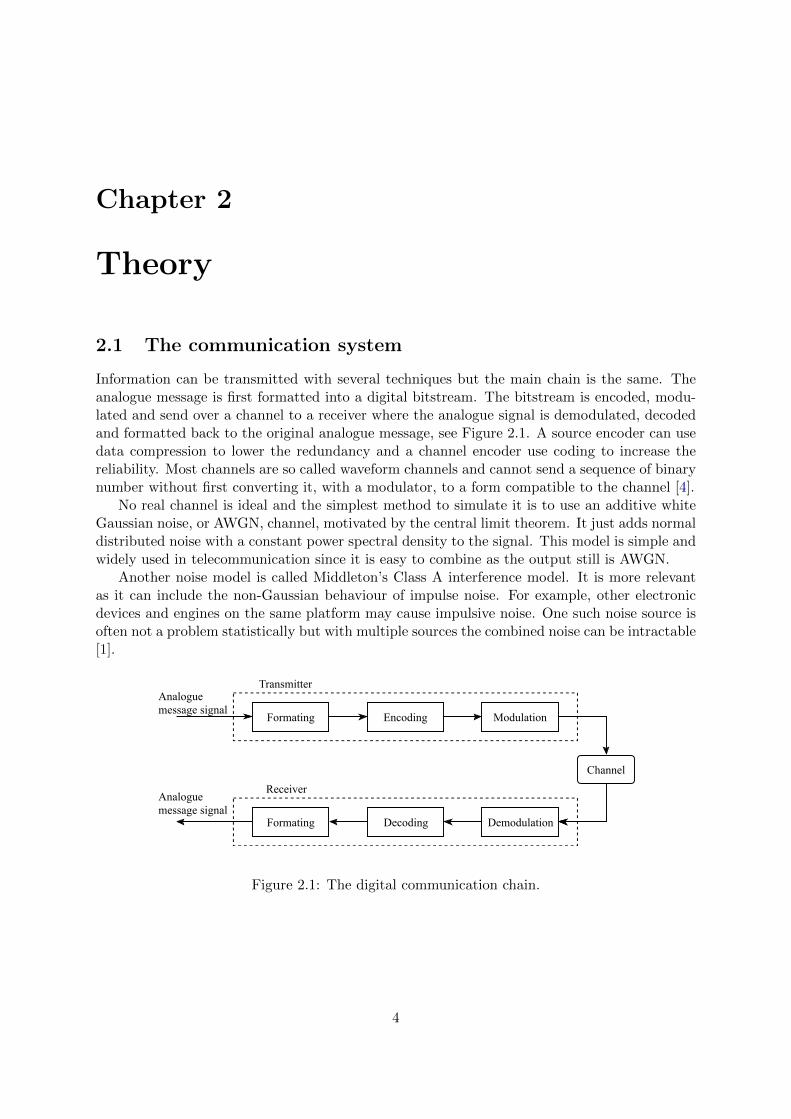
Information can be transmitted with several techniques but the main chain is the same. Theanalogue message is first formatted into a digital bitstream. The bitstream is encoded, modu-lated and send over a channel to a receiver where the analogue signal is demodulated, decodedand formatted back to the original analogue message, see Figure 2.1. A source encoder can usedata compression to lower the redundancy and a channel encoder use coding to increase thereliability. Most channels are so called waveform channels and cannot send a sequence of binarynumber without first converting it, with a modulator, to a form compatible to the channel [4].

No real channel is ideal and the simplest method to simulate it is to use an additive whiteGaussian noise, or AWGN, channel, motivated by the central limit theorem. It just adds normaldistributed noise with a constant power spectral density to the signal. This model is simple andwidely used in telecommunication since it is easy to combine as the output still is AWGN.

Another noise model is called Middleton’s Class A interference model. It is more relevantas it can include the non-Gaussian behaviour of impulse noise. For example, other electronicdevices and engines on the same platform may cause impulsive noise. One such noise source isoften not a problem statistically but with multiple sources the combined noise can be intractable[1].

Formating Encoding Modulation

Analoguemessage signal

Transmitter

Formating Decoding Demodulation

ReceiverAnaloguemessage signal

Channel

Figure 2.1: The digital communication chain.

4

2.2 Antennas

An antenna is an interface for transition between a guided and a free-space wave [5]. It is adevice for both transmitting and receiving of electromagnetic waves and the same model canoften be used for both cases since the device is reciprocal under most conditions, it is just amatter of convenience [6]. Although antenna comes in a wide variety they all operate accordingto the same rules of electromagnetics. Electromagnetic waves are oscillations of electric andmagnetic fields that transmits power at the speed of light and persist in absence of its source[7].

The simplest case of a transmitting antenna is a rod in which an alternating current isfed. As for a receiving antenna the incoming electromagnetic field pushes the electrons in therod back and forth and the created oscillating current is measured by the receiver. The saidantenna can be found in the large class of dipole antennas. A dipole antenna has two conductorsarranged symmetrically around a feeder, who typically is a quarter wavelength long. The dipolecan be connected to form larger structures such as Yagi-Uda which is a common antenna forterrestrial television receiving [8]. Another similar antenna type is monopole antenna in whichone conductor is omitted and replaced by a groundplane [7].

2.2.1 Directivity and gain

A hypothetical antenna that radiates equal power in all direction is called an isotropic antenna,and is often used as a reference when comparing antennas [6]. If a λ/2 dipole antenna is placedin free space the radiation pattern is rotationally symmetric in the perpendicular plane, with again of 2.15 dB compared to the isotropic case [5]. The total power emitted is the same but it isdistributed differently and for a dipole there is no power radiated in the extension of the dipoleaxis. In reality there is always some structure in the surrounding, anthropogenic or natural,that changes the pattern. Also worth mentioning is that antennas often are constructed toradiate in one particular direction, by using reflectors or several cooperating antennas. Thestrongest direction is often refered to as main lobe unlike side lobes and back lobe [7].

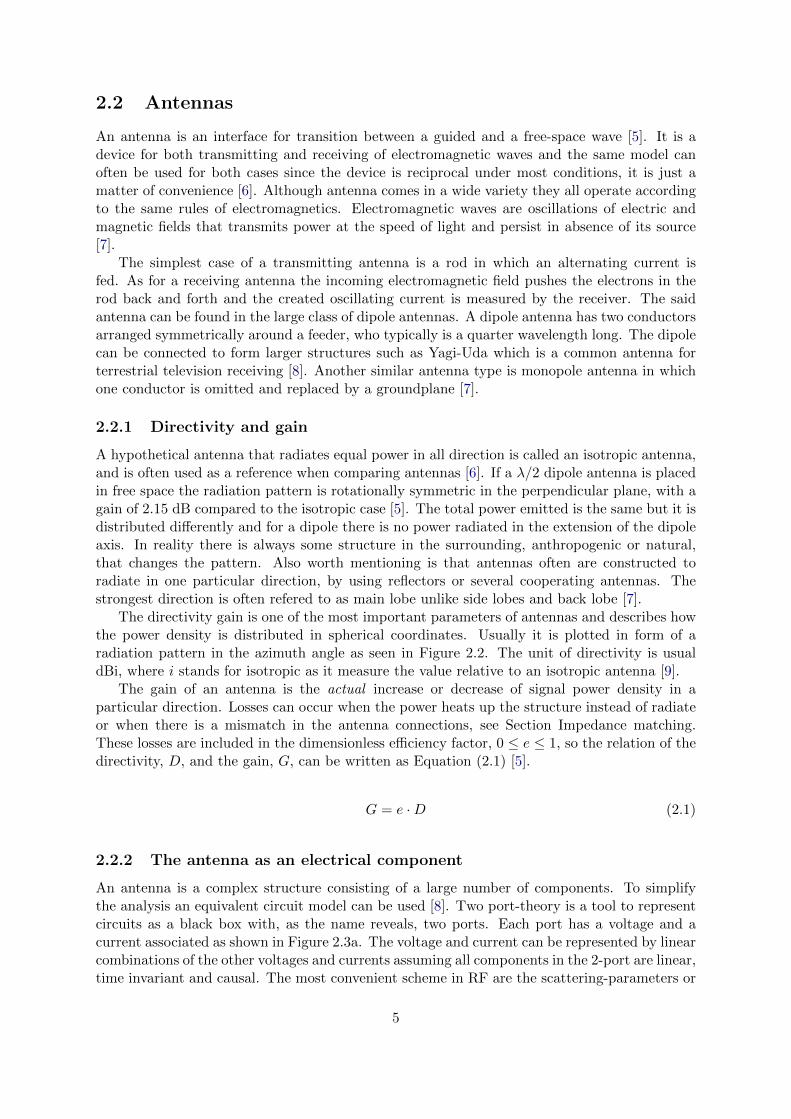
The directivity gain is one of the most important parameters of antennas and describes howthe power density is distributed in spherical coordinates. Usually it is plotted in form of aradiation pattern in the azimuth angle as seen in Figure 2.2. The unit of directivity is usualdBi, where i stands for isotropic as it measure the value relative to an isotropic antenna [9].

The gain of an antenna is the actual increase or decrease of signal power density in aparticular direction. Losses can occur when the power heats up the structure instead of radiateor when there is a mismatch in the antenna connections, see Section Impedance matching.These losses are included in the dimensionless efficiency factor, 0 ≤ e ≤ 1, so the relation of thedirectivity, D, and the gain, G, can be written as Equation (2.1) [5].

G = e ·D (2.1)

2.2.2 The antenna as an electrical component

An antenna is a complex structure consisting of a large number of components. To simplifythe analysis an equivalent circuit model can be used [8]. Two port-theory is a tool to representcircuits as a black box with, as the name reveals, two ports. Each port has a voltage and acurrent associated as shown in Figure 2.3a. The voltage and current can be represented by linearcombinations of the other voltages and currents assuming all components in the 2-port are linear,time invariant and causal. The most convenient scheme in RF are the scattering-parameters or

5

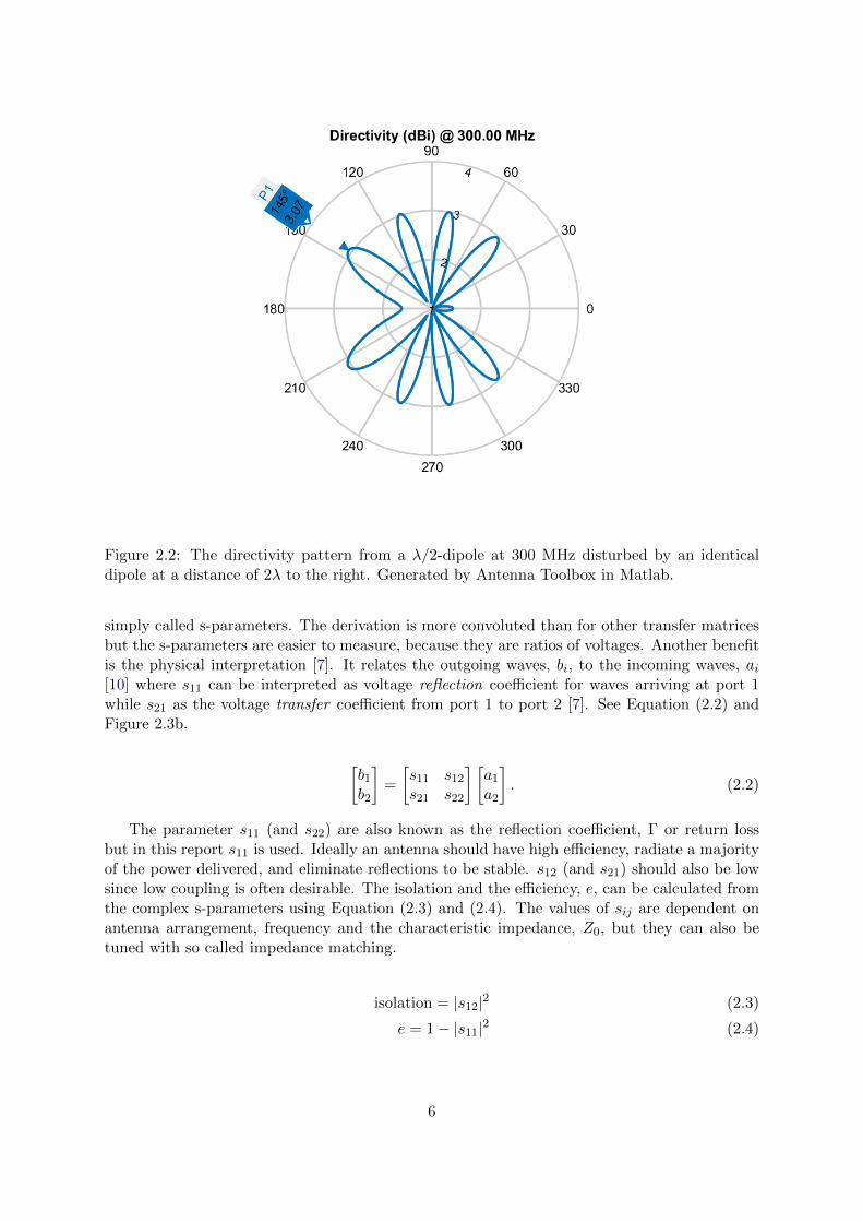
Figure 2.2: The directivity pattern from a λ/2-dipole at 300 MHz disturbed by an identicaldipole at a distance of 2λ to the right. Generated by Antenna Toolbox in Matlab.

simply called s-parameters. The derivation is more convoluted than for other transfer matricesbut the s-parameters are easier to measure, because they are ratios of voltages. Another benefitis the physical interpretation [7]. It relates the outgoing waves, bi, to the incoming waves, ai[10] where s11 can be interpreted as voltage reflection coefficient for waves arriving at port 1while s21 as the voltage transfer coefficient from port 1 to port 2 [7]. See Equation (2.2) andFigure 2.3b.

[b1b2

]=

[s11 s12s21 s22

] [a1a2

]. (2.2)

The parameter s11 (and s22) are also known as the reflection coefficient, Γ or return lossbut in this report s11 is used. Ideally an antenna should have high efficiency, radiate a majorityof the power delivered, and eliminate reflections to be stable. s12 (and s21) should also be lowsince low coupling is often desirable. The isolation and the efficiency, e, can be calculated fromthe complex s-parameters using Equation (2.3) and (2.4). The values of sij are dependent onantenna arrangement, frequency and the characteristic impedance, Z0, but they can also betuned with so called impedance matching.

isolation = |s12|2 (2.3)

e = 1− |s11|2 (2.4)

6

V1

I1 I2

+

­V2+

­

Text

(a)

Z0 Z0

a1b1

a2b2

(b)

Figure 2.3: (a) A two-port with voltages and currents. (b) Incoming, ai, and outgoing waves,bi, of the two-port where Z0 is characteristic impedance of the transmission line.

2.2.3 Impedance matching

Impedance matching is an important part of the design process of antennas and other electronicdevises. Impedance is measured in ohm, Ω, and has a real part and a complex part which isformed by a resistance respective and a reactance component. For DC transmission the complexpart is negligible but not for high frequencies as in a transmission line. When tuned incorrectlyradio frequencies, RF, may be reflected in joints as the medium has different properties. Asolution is to use impedance matching to minimize the reflection or to maximize the powertransfer.

Voltage Standing Wave Ratio or VSWR is a way to measure how well matched an antennaand a transmission line are and it is a function of the return loss, or s11-parameter, see Equation(2.5). Usually the VSWR should be lower than three which correspond to a |s11|2-value of -6dB, or an efficency of more than about 75 % [7].

VSWR =1 + |s11|1− |s11|

(2.5)

In impedance matching a matching network is placed between the transmission line and theport of the antenna. The transmission line is usually said to have a characteristic impedance,or Z0, of 50 Ω and the corresponding value of a λ/2-dipole antenna is 73 Ω. For example doesa value of 50 + 0j Ω mean that the magnitude of the forward voltage wave at a certain crosssection is 50 times higher than the current ditto. The phase shift, how much the current lagsthe voltage, is given by the the angle in the complex plane, which in this case is zero.

The voltage reflection coefficient of a junction is given by s11 = b2a1|a2=0 =

V o1

V i1

where V i1

and V o1 is forward and backward traveling voltage from port 1 seen in Figure 2.3. This ratio of

voltages equals to ZL−Z0ZL+Z0

and from this one can see that the line is matched if Z0 = ZL, sincethe reflection is zero [7].

L-section impedance matching

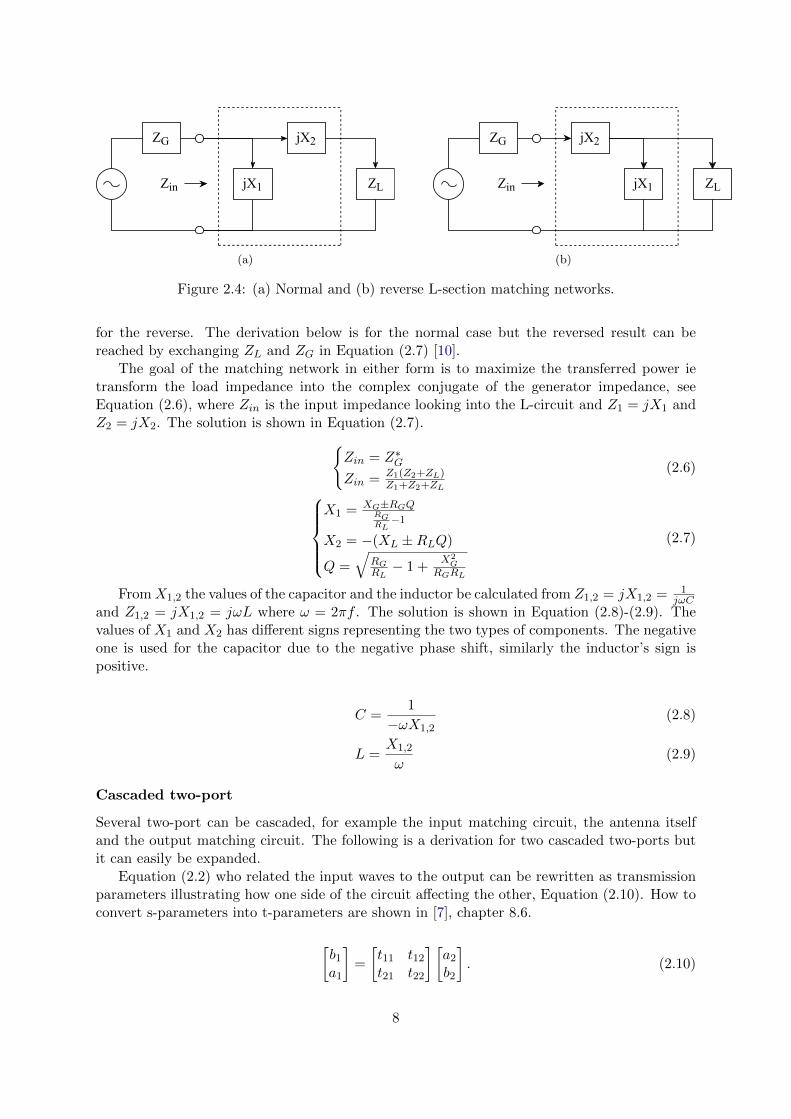
One of the simplest method to achieve matching, if just a narrow bandwidth is required, is to usefilters, for example the L-match circuit. It uses one inductor and one capacitor connecting thesource and the load as seen in Figure 2.4, where the complex load and generator impedances areZL = RL + jXL and ZG = RG + jXG. The figure shows both normal and reversed L-section, tobe used under different conditions. A guideline is to use the normal for RG > RL and opposite

7

ZG jX2

ZLjX1Zin

(a)

ZG jX2

ZLjX1Zin

Text

(b)

Figure 2.4: (a) Normal and (b) reverse L-section matching networks.

for the reverse. The derivation below is for the normal case but the reversed result can bereached by exchanging ZL and ZG in Equation (2.7) [10].

The goal of the matching network in either form is to maximize the transferred power ietransform the load impedance into the complex conjugate of the generator impedance, seeEquation (2.6), where Zin is the input impedance looking into the L-circuit and Z1 = jX1 andZ2 = jX2. The solution is shown in Equation (2.7).

Zin = Z∗G

Zin = Z1(Z2+ZL)Z1+Z2+ZL

(2.6)

X1 = XG±RGQ

RGRL

−1

X2 = −(XL ±RLQ)

Q =

√RGRL− 1 +

X2G

RGRL

(2.7)

FromX1,2 the values of the capacitor and the inductor be calculated from Z1,2 = jX1,2 = 1jωC

and Z1,2 = jX1,2 = jωL where ω = 2πf . The solution is shown in Equation (2.8)-(2.9). Thevalues of X1 and X2 has different signs representing the two types of components. The negativeone is used for the capacitor due to the negative phase shift, similarly the inductor’s sign ispositive.

C =1

−ωX1,2(2.8)

L =X1,2

ω(2.9)

Cascaded two-port

Several two-port can be cascaded, for example the input matching circuit, the antenna itselfand the output matching circuit. The following is a derivation for two cascaded two-ports butit can easily be expanded.

Equation (2.2) who related the input waves to the output can be rewritten as transmissionparameters illustrating how one side of the circuit affecting the other, Equation (2.10). How toconvert s-parameters into t-parameters are shown in [7], chapter 8.6.

[b1a1

]=

[t11 t12t21 t22

] [a2b2

]. (2.10)

8

If connecting two two-port after each other, the output port of the first equals the input

port of the second, ie a(1)2 = b

(2)1 and b

(1)2 = a

(2)1 , so the system can be rewritten as a sum of

transmission matrices, as in Equation (2.11). The cascaded s-parameters are then obtained byre-converting the new t-matrix using [7].

[b(1)1

a(1)1

]=

[t(1)11 t

(1)12

t(1)21 t

(1)22

][t(2)11 t

(2)12

t(2)21 t

(2)22

][a(2)2

b(2)2

]. (2.11)

2.3 Signal, noise and interference

Signals measured at a receiver are often weak due to attenuation but since the receiver usuallyhas a high amplification it is not a particular problem. What causes more problem is noise,interference and other disturbances [8]. In wireless communication SNR is an important param-eter. SNR stands for signal-to-noise ratio and is the power of the signal compared to the powerof the noise. Similar quantities are SIR, signal-to-interference ratio and signal-to-interference-plus-noise ratio, SINR.

The received power is a function of the transmitted power, Pt, as well as the gain of transmitand receive antenna, Gt and Gr. The loss the signal suffers on its way is called the elementarypath loss, Lb [8]. The noise power is often calculated as thermal noise, dependent on Boltzmann’sconstant, k and the absolute temperature of the component, T . The total noise is measuredover the bandwidth, B, and also includes F , which is locally generated noise and the noisefactor of the receiver. The total SNR is therefore shown in Equation (2.12) [2].

SNR =Psignal

Pnoise=

PtGtGr

LbkT0FB(2.12)

An ideal transmitter is just broadcasting in the intended frequency range but in reality thepower is also leaking to the adjacent frequencies. The term sideband is used to describe howmany channel to each side of the center frequency that are affected over a considerable level.The level and spread of the disturbance is effected by modulation method, filtering and phasenoise among others. This power can be measured in relation to the main frequency, commonlyin dB and there are standards specifying requirements for different applications [2].

The SIR calculation is using the same function for signal power as SNR. The interferedpower is also using the same form, as the interference is received power but from an unwantedsource. The elementary path loss is however replaced with the isolation and the noise poweris attenuated if the disturbing source is sending on a sideband. This can be simplified, seeEquation (2.13), where Pd is the power of the transmitter which is disturbing.

SIR =Psignal

Pinterference=

PtGtGrLb

Pd·attenuationisolation

(2.13)

The SINR, Equation (2.14), gives the theoretical upper bound of the channel capacity sinceit captures both interference and noise. If no interference, the equation equals the SNR and theother way around. The lowest value of SNR or SIR is the one affecting the most.

SINR =Psignal

Pnoise + Pinterference=

11

SNR + 1SIR

(2.14)

9

2.4 Frequency hopping system

A frequency hopping system uses techniques from both time and frequency multiplexing. Theavailable bandwidth is divided into narrower channels and the time is divided into slots. Forevery time slot the transmitter changes frequency according to a predefined hop sequence alsoknown by the receiver. Several transmitters can be active in the same frequency range and ifthe hopping sequences are chosen so the slots does not overlap, the system is orthogonal [8].

There are two main drawbacks of frequency hopping systems; the need for accurate timesynchronisation and frequency selectivity. However the technique are resistant to disturbances.In a Rayleigh fading environment where deeps nulls can occur locally at a single frequency,frequency hopping in combination with coding can decrease the errors as a missing part ofa codeword are able to recover. In military communication systems the ability to withstandinterference are of great importance both by intentional disturbance from an enemy or byunintentional interference from neighbouring platforms [8].

The probability of using the same frequency as another transmitter is a function of thenumber of frequencies available, nf , see Equation (2.15). The probability of using a frequencywhich are affected by the other transmitters sidebands is given in Equation (2.16) where s is thenumber of sidebands on one side of the center frequency of the interfering transmitter. The sameprobability but for orthogonal frequency hopping is given in Equation (2.17). All equations arefor two transmitters and are motivated in Appendix A.

pcollision(nf ) =1

nf(2.15)

psideband,FH(nf , s) =(nf − 2s)2s+ 2 ·

∑2s−1i=s i

n2f(2.16)

psideband,O-FH(nf , s) =(nf − 2s)2s+ 2 ·

∑2s−1i=s i

(nf − 1)nf(2.17)

10

Chapter 3

Antenna setup

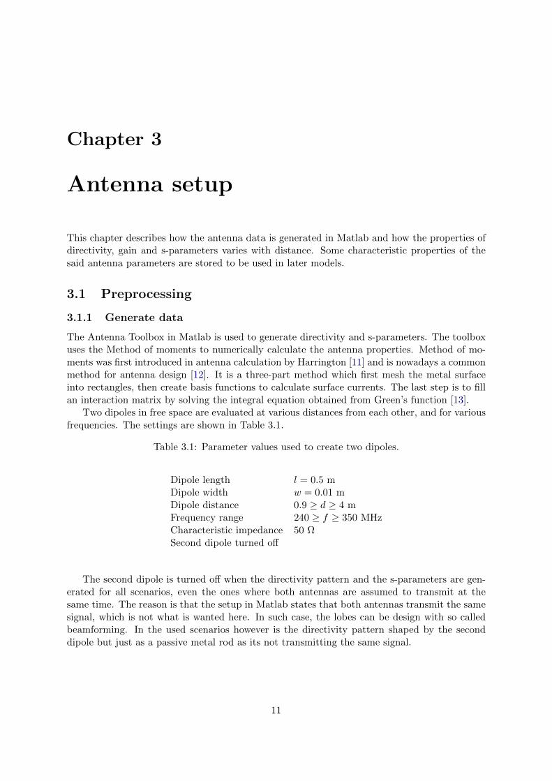
This chapter describes how the antenna data is generated in Matlab and how the properties ofdirectivity, gain and s-parameters varies with distance. Some characteristic properties of thesaid antenna parameters are stored to be used in later models.

3.1 Preprocessing

3.1.1 Generate data

The Antenna Toolbox in Matlab is used to generate directivity and s-parameters. The toolboxuses the Method of moments to numerically calculate the antenna properties. Method of mo-ments was first introduced in antenna calculation by Harrington [11] and is nowadays a commonmethod for antenna design [12]. It is a three-part method which first mesh the metal surfaceinto rectangles, then create basis functions to calculate surface currents. The last step is to fillan interaction matrix by solving the integral equation obtained from Green’s function [13].

Two dipoles in free space are evaluated at various distances from each other, and for variousfrequencies. The settings are shown in Table 3.1.

Table 3.1: Parameter values used to create two dipoles.

Dipole length l = 0.5 mDipole width w = 0.01 mDipole distance 0.9 ≥ d ≥ 4 mFrequency range 240 ≥ f ≥ 350 MHzCharacteristic impedance 50 ΩSecond dipole turned off

The second dipole is turned off when the directivity pattern and the s-parameters are gen-erated for all scenarios, even the ones where both antennas are assumed to transmit at thesame time. The reason is that the setup in Matlab states that both antennas transmit the samesignal, which is not what is wanted here. In such case, the lobes can be design with so calledbeamforming. In the used scenarios however is the directivity pattern shaped by the seconddipole but just as a passive metal rod as its not transmitting the same signal.

11

3.1.2 Impedance matching

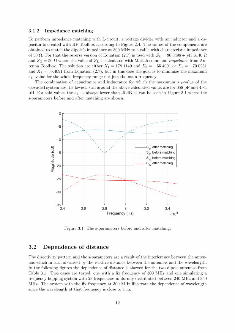
To perform impedance matching with L-circuit, a voltage divider with an inductor and a ca-pacitor is created with RF Toolbox according to Figure 2.4. The values of the components areobtained to match the dipole’s impedance at 300 MHz to a cable with characteristic impedanceof 50 Ω. For that the reverse version of Equation (2.7) is used with ZL = 90.3498 + j43.6140 Ωand ZG = 50 Ω where the value of ZL is calculated with Matlab command impedance from An-tenna Toolbox. The solution are either X1 = 178.1149 and X2 = −55.4091 or X1 = −70.0251and X2 = 55.4091 from Equation (2.7), but in this case the goal is to minimize the maximums11-value for the whole frequency range not just the main frequency.

The combination of capacitance and inductance for which the maximum s11-value of thecascaded system are the lowest, still around the above calculated value, are for 658 pF and 4.84µH. For said values the s11 is always lower than -6 dB as can be seen in Figure 3.1 where thes-parameters before and after matching are shown.

Figure 3.1: The s-parameters before and after matching.

3.2 Dependence of distance

The directivity pattern and the s-parameters are a result of the interference between the anten-nas which in turn is caused by the relative distance between the antennas and the wavelength.In the following figures the dependence of distance is showed for the two dipole antennas fromTable 3.1. Two cases are tested, one with a fix frequency of 300 MHz and one simulating afrequency hopping system with 23 frequencies uniformly distributed between 240 MHz and 350MHz. The system with the fix frequency at 300 MHz illustrate the dependence of wavelengthsince the wavelength at that frequency is close to 1 m.

12

3.2.1 s-parameters

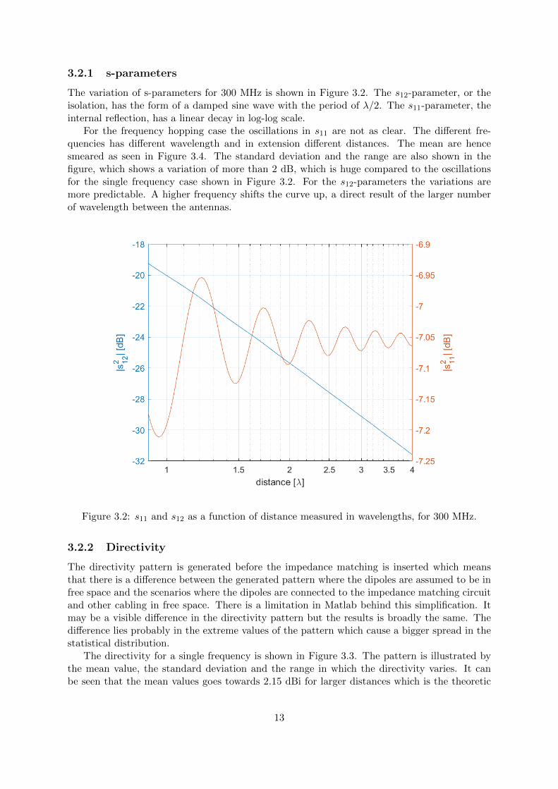
The variation of s-parameters for 300 MHz is shown in Figure 3.2. The s12-parameter, or theisolation, has the form of a damped sine wave with the period of λ/2. The s11-parameter, theinternal reflection, has a linear decay in log-log scale.

For the frequency hopping case the oscillations in s11 are not as clear. The different fre-quencies has different wavelength and in extension different distances. The mean are hencesmeared as seen in Figure 3.4. The standard deviation and the range are also shown in thefigure, which shows a variation of more than 2 dB, which is huge compared to the oscillationsfor the single frequency case shown in Figure 3.2. For the s12-parameters the variations aremore predictable. A higher frequency shifts the curve up, a direct result of the larger numberof wavelength between the antennas.

Figure 3.2: s11 and s12 as a function of distance measured in wavelengths, for 300 MHz.

3.2.2 Directivity

The directivity pattern is generated before the impedance matching is inserted which meansthat there is a difference between the generated pattern where the dipoles are assumed to be infree space and the scenarios where the dipoles are connected to the impedance matching circuitand other cabling in free space. There is a limitation in Matlab behind this simplification. Itmay be a visible difference in the directivity pattern but the results is broadly the same. Thedifference lies probably in the extreme values of the pattern which cause a bigger spread in thestatistical distribution.

The directivity for a single frequency is shown in Figure 3.3. The pattern is illustrated bythe mean value, the standard deviation and the range in which the directivity varies. It canbe seen that the mean values goes towards 2.15 dBi for larger distances which is the theoretic

13

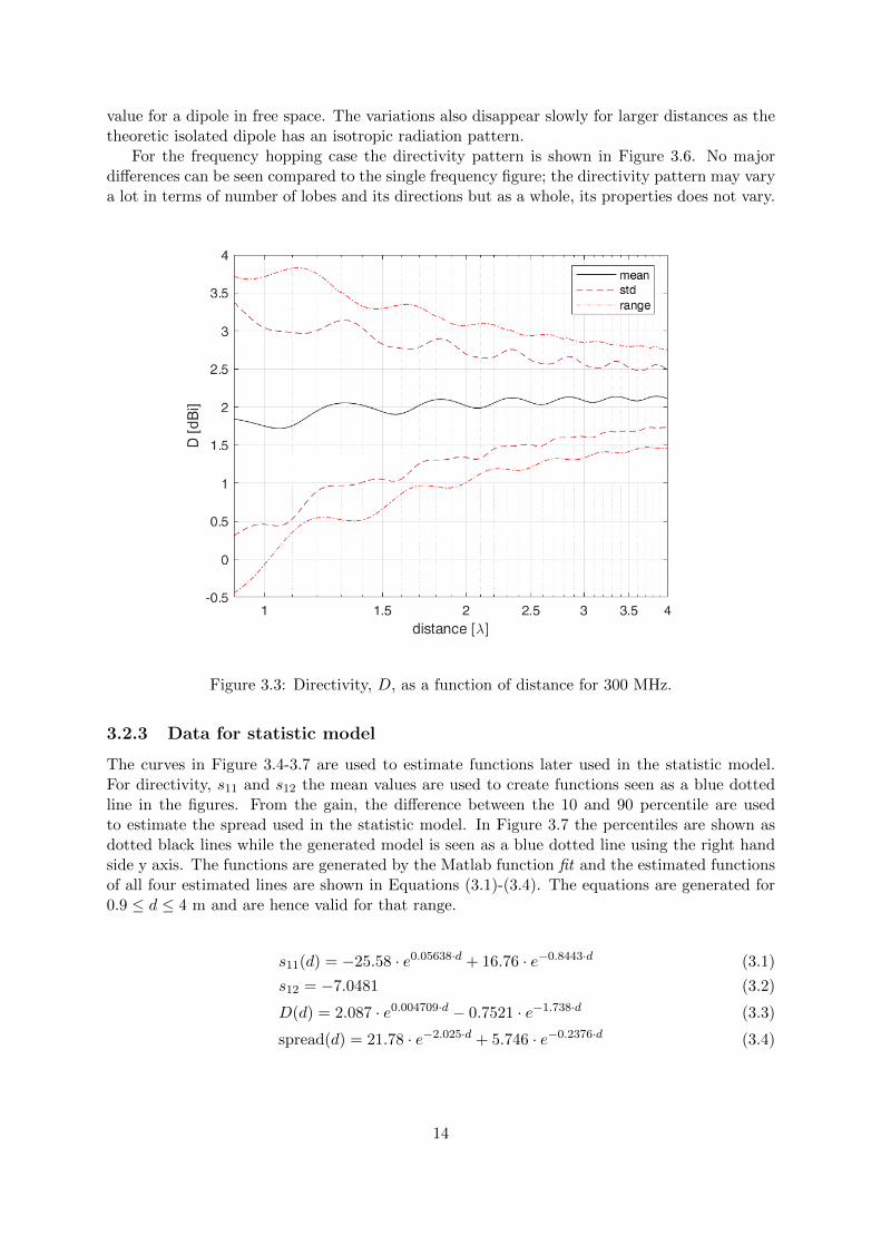
value for a dipole in free space. The variations also disappear slowly for larger distances as thetheoretic isolated dipole has an isotropic radiation pattern.

For the frequency hopping case the directivity pattern is shown in Figure 3.6. No majordifferences can be seen compared to the single frequency figure; the directivity pattern may varya lot in terms of number of lobes and its directions but as a whole, its properties does not vary.

Figure 3.3: Directivity, D, as a function of distance for 300 MHz.

3.2.3 Data for statistic model

The curves in Figure 3.4-3.7 are used to estimate functions later used in the statistic model.For directivity, s11 and s12 the mean values are used to create functions seen as a blue dottedline in the figures. From the gain, the difference between the 10 and 90 percentile are usedto estimate the spread used in the statistic model. In Figure 3.7 the percentiles are shown asdotted black lines while the generated model is seen as a blue dotted line using the right handside y axis. The functions are generated by the Matlab function fit and the estimated functionsof all four estimated lines are shown in Equations (3.1)-(3.4). The equations are generated for0.9 ≤ d ≤ 4 m and are hence valid for that range.

s11(d) = −25.58 · e0.05638·d + 16.76 · e−0.8443·d (3.1)

s12 = −7.0481 (3.2)

D(d) = 2.087 · e0.004709·d − 0.7521 · e−1.738·d (3.3)

spread(d) = 21.78 · e−2.025·d + 5.746 · e−0.2376·d (3.4)

14

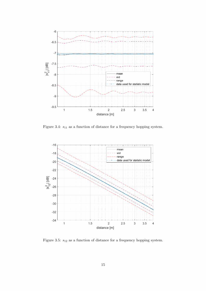
Figure 3.4: s11 as a function of distance for a frequency hopping system.

Figure 3.5: s12 as a function of distance for a frequency hopping system.

15

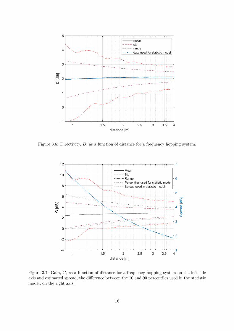
Figure 3.6: Directivity, D, as a function of distance for a frequency hopping system.

Figure 3.7: Gain, G, as a function of distance for a frequency hopping system on the left sideaxis and estimated spread, the difference between the 10 and 90 percentiles used in the statisticmodel, on the right axis.

16

Chapter 4

The model

4.1 Simulation setup

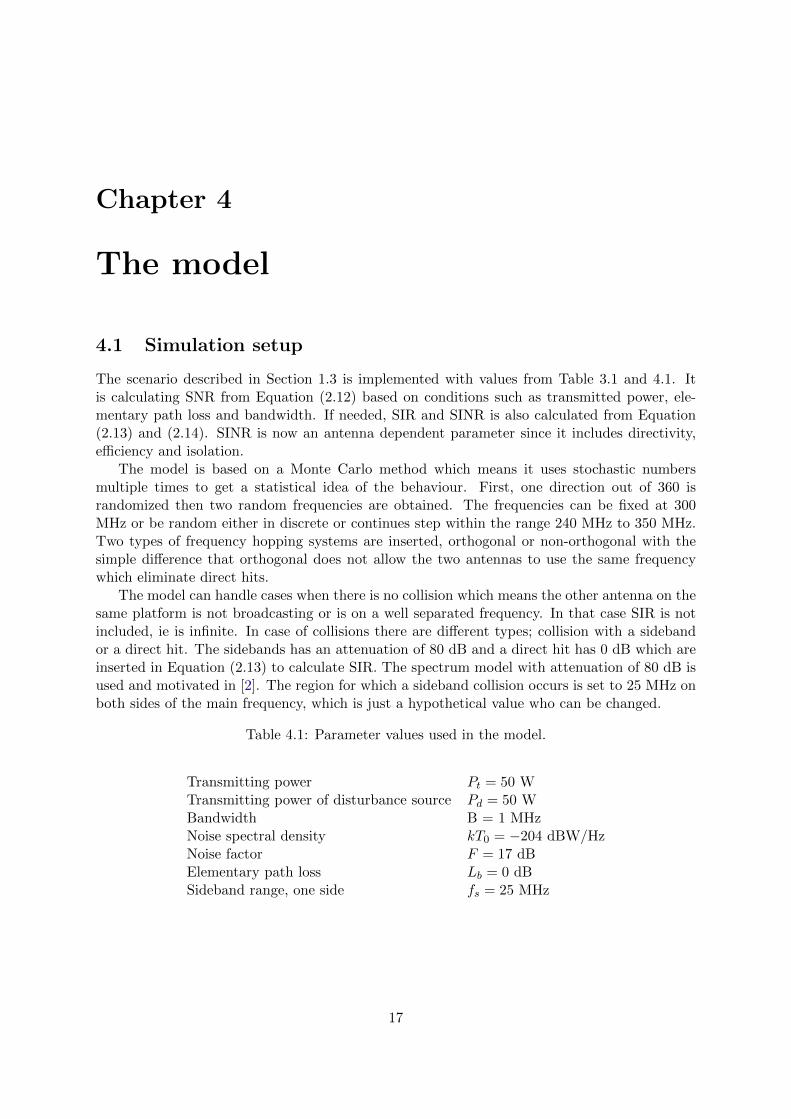
The scenario described in Section 1.3 is implemented with values from Table 3.1 and 4.1. Itis calculating SNR from Equation (2.12) based on conditions such as transmitted power, ele-mentary path loss and bandwidth. If needed, SIR and SINR is also calculated from Equation(2.13) and (2.14). SINR is now an antenna dependent parameter since it includes directivity,efficiency and isolation.

The model is based on a Monte Carlo method which means it uses stochastic numbersmultiple times to get a statistical idea of the behaviour. First, one direction out of 360 israndomized then two random frequencies are obtained. The frequencies can be fixed at 300MHz or be random either in discrete or continues step within the range 240 MHz to 350 MHz.Two types of frequency hopping systems are inserted, orthogonal or non-orthogonal with thesimple difference that orthogonal does not allow the two antennas to use the same frequencywhich eliminate direct hits.

The model can handle cases when there is no collision which means the other antenna on thesame platform is not broadcasting or is on a well separated frequency. In that case SIR is notincluded, ie is infinite. In case of collisions there are different types; collision with a sidebandor a direct hit. The sidebands has an attenuation of 80 dB and a direct hit has 0 dB which areinserted in Equation (2.13) to calculate SIR. The spectrum model with attenuation of 80 dB isused and motivated in [2]. The region for which a sideband collision occurs is set to 25 MHz onboth sides of the main frequency, which is just a hypothetical value who can be changed.

Table 4.1: Parameter values used in the model.

Transmitting power Pt = 50 WTransmitting power of disturbance source Pd = 50 WBandwidth B = 1 MHzNoise spectral density kT0 = −204 dBW/HzNoise factor F = 17 dBElementary path loss Lb = 0 dBSideband range, one side fs = 25 MHz

17

4.2 Antenna models

Three different antenna models are implemented, all using its own values for directivity ands-parameters. One using data generated by Matlab, one using an isotropic model, and onemodel tries to mimic the behaviour of the system, and still be simple. All models except thelatter uses Monte Carlo simulations.

4.2.1 Matlab model

This model is using data generated from the Antenna Toolbox for the settings in Table 3.1.Thismodel is assumed to be correct, but as simplified as its input data. To obtain frequencies inbetween the generated frequencies with spacing 5 MHz, interpolation is used.

4.2.2 Previously used models - isotropic

The simplest possible model is to set the gains, Gt and Gr in Equation (2.12) to 0 dB. A slightlymore advanced model is to assume efficiency of one and an isotope radiation pattern which fora dipole has a directivity of 2.15 dBi. Both is used here together with a constant isolation of -25dB. The former is used for comparison as it symbols the system where the antenna is completelyremoved.

4.2.3 Statistic model

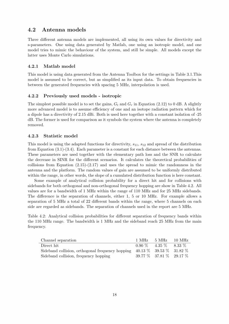
This model is using the adapted functions for directivity, s11, s12 and spread of the distributionfrom Equation (3.1)-(3.4). Each parameter is a constant for each distance between the antennas.These parameters are used together with the elementary path loss and the SNR to calculatethe decrease in SINR for the different scenarios. It calculates the theoretical probabilities ofcollisions from Equation (2.15)-(2.17) and uses the spread to mimic the randomness in theantenna and the platform. The random values of gain are assumed to be uniformly distributedwithin the range, in other words, the slope of a cumulated distribution function is here constant.

Some example of analytical collision probability for a direct hit and for collisions withsidebands for both orthogonal and non-orthogonal frequency hopping are show in Table 4.2. Allvalues are for a bandwidth of 1 MHz within the range of 110 MHz and for 25 MHz sidebands.The difference is the separation of channels, either 1, 5 or 10 MHz. For example allows aseparation of 5 MHz a total of 22 different bands within the range, where 5 channels on eachside are regarded as sidebands. The separation of channels used in the report are 5 MHz.

Table 4.2: Analytical collision probabilities for different separation of frequency bands withinthe 110 MHz range. The bandwidth is 1 MHz and the sideband reach 25 MHz from the mainfrequency.

Channel separation 1 MHz 5 MHz 10 MHz

Direct hit 0.90 % 4.35 % 8.33 %Sideband collision, orthogonal frequency hopping 40.13 % 39.53 % 31.82 %Sideband collision, frequency hopping 39.77 % 37.81 % 29.17 %

18

Chapter 5

Comparison of models

5.1 Overview

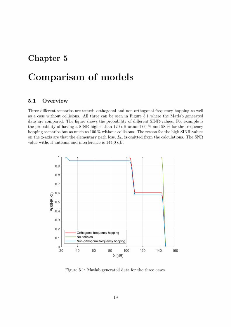
Three different scenarios are tested: orthogonal and non-orthogonal frequency hopping as wellas a case without collisions. All three can be seen in Figure 5.1 where the Matlab generateddata are compared. The figure shows the probability of different SINR-values. For example isthe probability of having a SINR higher than 120 dB around 60 % and 58 % for the frequencyhopping scenarios but as much as 100 % without collisions. The reason for the high SINR-valueson the x-axis are that the elementary path loss, Lb, is omitted from the calculations. The SNRvalue without antenna and interference is 144.0 dB.

Figure 5.1: Matlab generated data for the three cases.

19

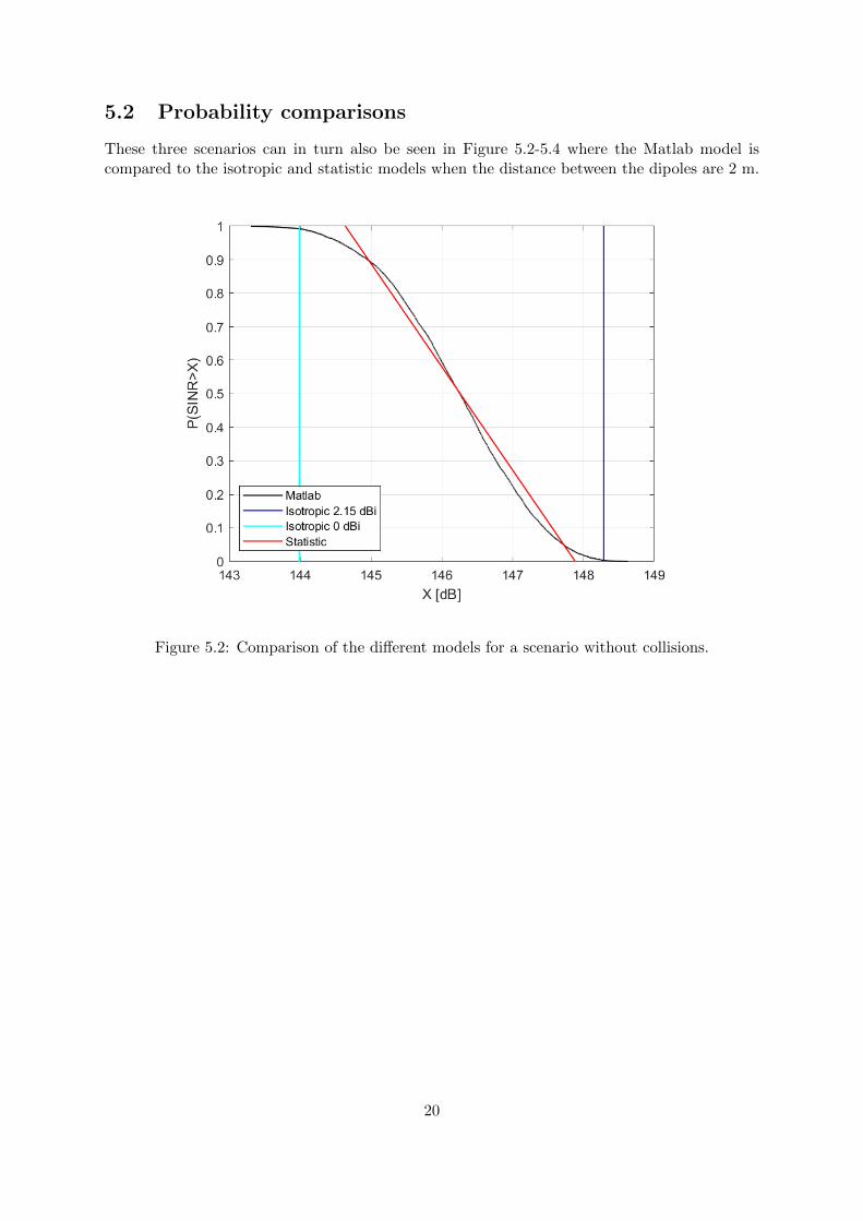
5.2 Probability comparisons

These three scenarios can in turn also be seen in Figure 5.2-5.4 where the Matlab model iscompared to the isotropic and statistic models when the distance between the dipoles are 2 m.

Figure 5.2: Comparison of the different models for a scenario without collisions.

20

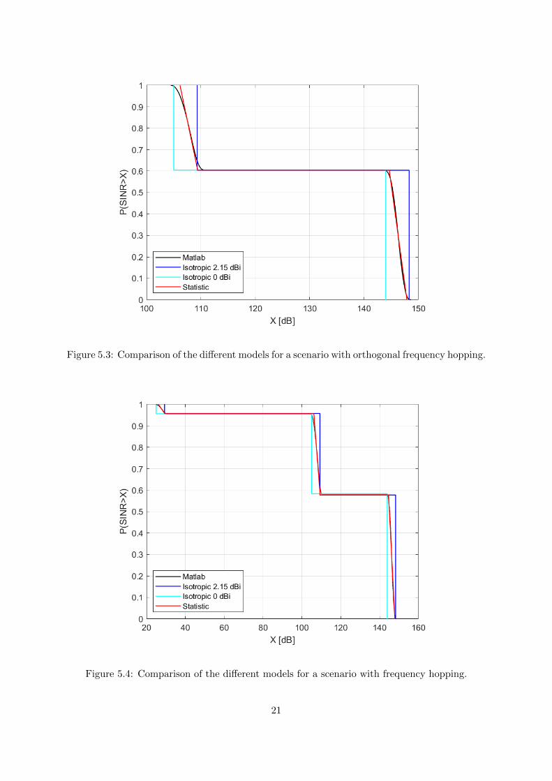
Figure 5.3: Comparison of the different models for a scenario with orthogonal frequency hopping.

Figure 5.4: Comparison of the different models for a scenario with frequency hopping.

21

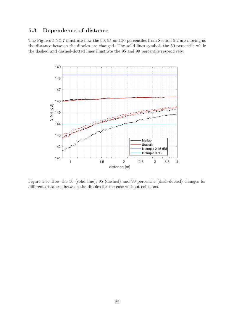
5.3 Dependence of distance

The Figures 5.5-5.7 illustrate how the 99, 95 and 50 percentiles from Section 5.2 are moving asthe distance between the dipoles are changed. The solid lines symbols the 50 percentile whilethe dashed and dashed-dotted lines illustrate the 95 and 99 percentile respectively.

Figure 5.5: How the 50 (solid line), 95 (dashed) and 99 percentile (dash-dotted) changes fordifferent distances between the dipoles for the case without collisions.

22

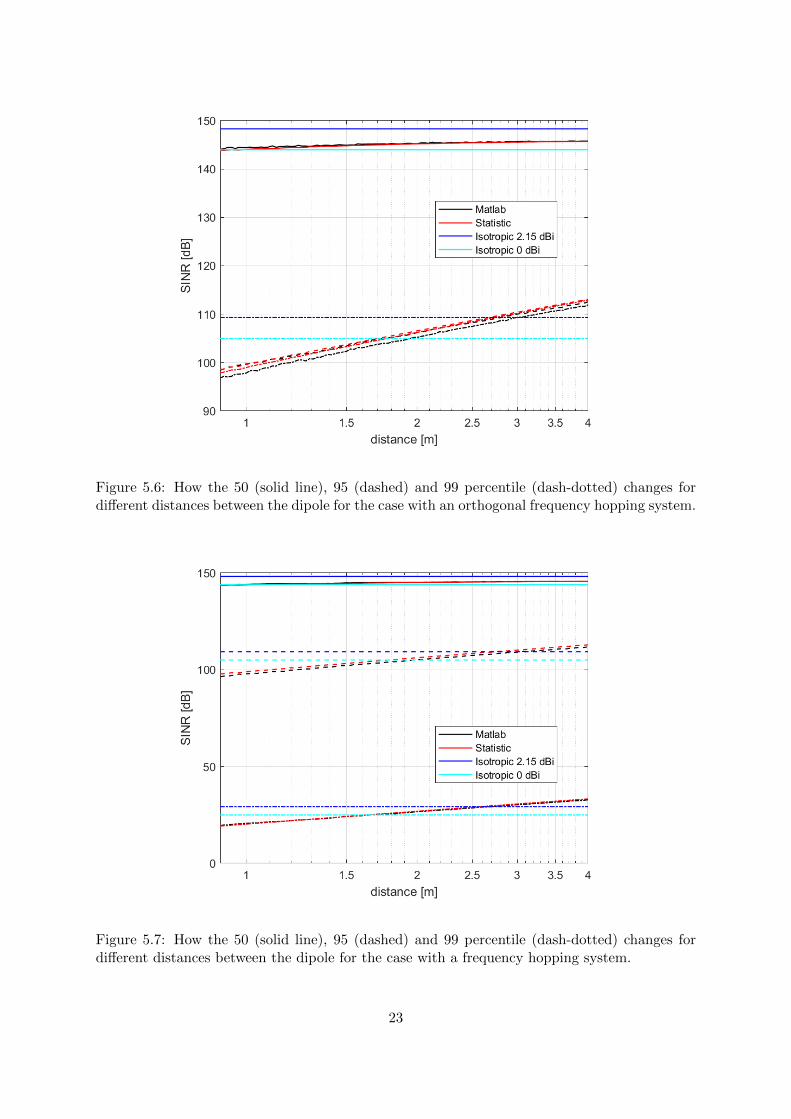
Figure 5.6: How the 50 (solid line), 95 (dashed) and 99 percentile (dash-dotted) changes fordifferent distances between the dipole for the case with an orthogonal frequency hopping system.

Figure 5.7: How the 50 (solid line), 95 (dashed) and 99 percentile (dash-dotted) changes fordifferent distances between the dipole for the case with a frequency hopping system.

23

Chapter 6

Discussion

The impact of the antenna, seen as a system component integrated on a platform for frequencyhopping radio links is something which is not well investigated. It is however of great interest asthe antenna is an important part and can affect the throughput significantly if poorly integratedon the platform. The model used in this report is very simplified but can still give an insight ofits behaviour, even though its values and figures should not be used as truth, just guidelines,for future projects.

The questions that will be discussed below are,

• How the radiolink performance is affected by the antenna in frequency hopping systems.

• How good the frequently used isotopic antenna model is.

• If it is possible to create a simple model to mimic the statistical performance of theantenna.

as well as the models reliability and when and how it can be used. The delimitations taken intoaccount when creating the model is discussed and ideas for future extensions are given.

6.1 Discussion of models

6.1.1 Matlab model

• How the radiolink performance is affected by the antenna in frequency hopping systems.

Both the internal reflection, the isolation and the directivity is affecting the SINR-value inthis model. This simplified case has just two dipole antennas in free space but the values areaffected by the number of wavelength between the antennas and, for the directivity, also bythe direction. For a frequency hopping system, this leads to a complex model in which thefrequency and hence also the number of wavelengths between the antennas, changes constantly.

Impedance matching is used in this report to lower the highest s11 parameter to a valuebelow -6 dB, to be more realistic but it is also a factor affecting the performance. The reporthas showed that s11, s12 and directivity are all important in determining the SINR. Anothertype of impedance matching may lower s11 and s12 with several dB which of course will have aimpact on the end results.

Another important aspect of the model is the impact of several frequency hopping systems onthe same platform. The probability that two systems simultaneously uses the same frequency is afunction of the available hopping frequencies and the SINR decreases significantly for frequency

24

collisions. Even collision with a sideband affect the SINR. In this cases the sidebands aremodelled with a simple model where all sideband has a attenuation of -80 dB. This is also anunrealistic simplification but it shows the general trend.

The parameters which affects the antenna are internal reflection, isolation and directivitypattern. Both the internal reflection and the directivity affect the antenna gain which causesa spread of SINR of around 4 dB in this case. To know about this spread may be importantas the worst percentiles is relevant when calculating which throughput that can be guaranteed.Every decibel of isolations increase the SINR by one decibel for the collisions and is hence alsorelevant.

The choice of orthogonal and non-orthogonal frequency hopping and how many hoppingfrequencies are parameters which affect the throughput even more according to this simplifiedmodel. Important is the spectrum and how the attenuation of neighbouring frequencies increase.

This model is realistic for the scenarios described as Matlab uses Method of Moments whichin general gives accurate results. What is not realistic are the simplifications such antenna setup,spectrum model or parameter values and the model is not better than its settings. The antennacalculation complexity increase however for additional features as antennas and groundplaneand it may lead to timeconsuming calculations. Generally it can be assumed that more complexinput data causes a larger spread.

6.1.2 Isotropic model

• How good the frequently used isotopic antenna model is.

The two isotropic antenna models, the with gain of one and with gain of 2.15 dBi, areenclosing the Matlab generated gain distribution as seen in Figure 5.2 where the former modelhas a SNR of 144.0 dB and the latter 148.3 dB. Not regarding the antenna at all produce anaverage SNR of around 2 dB lower than the Matlab generated and the optimistic model withgain of 2.15 dBi produces in turn a higher SNR. Both models are wrong in aspect of distributionand mean value compared to the Matlab model. The variation of around 4 dB is not includedand even if the mean value are correct, the true model can result in lower throughput thanpredicted due to the spread. The isotropic model does not either take into account that thedistance between the dipole can change. From Figures 5.5-5.7 it can be seen that the differencebetween the Matlab model and the isotropic model varies with distance.

Disregarding the lack of spread, both isotropic models are relatively good, at least whencompared to its complexity. It can be used to see effect from frequency hopping and visualisehow actions affect the system.

6.1.3 Statistical model

• If it is possible to create a simple model to mimic the statistical performance of theantenna.

A very simple model was created from the mean value of directivity, s11, s12 and from thespread of the gain. This model show promising results as it mimics the spread of the antennais a way the isotropic model can not. It is also able to capture the behaviour as the distancebetween the antennas are changed in a way the isotropic models is not. Another benefit of themodel is that it can be used to predict the impact from the antenna in the scenarios withouthaving to do any time consuming Monte Carlo loops of calculations. It is promising that justfour estimated constants can be used to calculate the behaviour of the antenna in the triedscenarios, and even mimic the distance dependent relationship. What should be remembered

25

is that the Matlab data was used to obtain the constants so the conformity cannot be fairlyanalysed.

Useful in this model is also the theoretical probability of collision with sideband for frequencyhopping systems. Previously used models, for example in [2], was using a simplified model whodid not regard probability of hitting a sideband of an edge frequency. The model in this reportis theoretically correct for this simplified model, and it can with minor work be used in futurereports.

6.2 Discussion of method

The antenna setup in this model with two identical dipole antennas in free space, is an unrealcase. Also the spectrum model, the values of the antenna parameters which is assumptions andthe Monte Carlo model where the platforms are changing direction randomly for every frequencyhop. Neither of this is very realistic but it is a first step to create a model which can be expanded.It is also a way to identify the most important antenna properties for radio communication.The same applies for coding, electromagnetical properties, fading or non-Gaussian noise, whichis not discussed.

6.3 Future work

In this thesis project the most simple model is used as proof of concept. No actual values areused as antenna size, shape, setup nor as frequency range, spectrum model or other parameters.The values are realistic but are assumptions or simplifications. The next step would be touse realistic values. It would be interesting to see the agreement between measurements ofdirectivity and the Matlab model as the measurement are difficult of obtain, but relativelysimple to calculate in Matlab. The s-parameters are easier to measure and maybe the measuredvalues can be used in later models together with an assumed spread to increase the conformity.

26

Chapter 7

Conclusion

In this degree project some antenna parameters are inserted into a Matlab model to evaluatethe impact of the antenna in a frequency hopping system. The model is simple but still showsthat it is possible to create a model from Antenna Toolbox data. It also shows general trendssuch as how the directivity and s-parameters affect the system.

The two isotropic models often used are simple but has a quite good conformity. A createdstatistical model shows that only a few properties is needed to mimic the statistical behaviourof the antenna to a certain degree. This comparison is done relative to the Matlab data, whichwas used to create the model, so the model should be used with care but the created modelis likely better than the isotropic models as it includes the statistic spread and also followsthe dipole distance dependence. This model can be used as a first model to test other designparameters.

The next step would be to adapt for real scenarios with for example other spectrum models,real s-parameters or actual system parameters. A comparison with real measurement is alsodesired. If the Matlab model can be expanded so that the conformity with real measurement isgood, the simulation can be used instead which saves resources.

27

Bibliography

[1] S. O. Tengstrand, P. Eliardsson, E. Axell, B. Johansson, K. Wiklundh, Methods for Valuationof Measures that Increase Robustness of Wireless Communication Systems. Technical ReportFOI-R–4302–SE, FOI, 2016.

[2] K. Fors and S. Linder, Konsekvenser av interferensmiljon vid samgruppering av frekven-shoppande radiosystem, FOI-R–4318–SE, FOI, 2016.

[3] T. Lindgren, Simulation of the performance of communication antenna systems integratedon platforms. Technical Report FOI-R–4221–SE, FOI, 2016.

[4] J. G. Proakis, Digital Communication, McGraw-Hill Book Company, USA, 1989.

[5] J. D. Kraus, R. J. Marhefka, Antennas For All Applications, McGraw-Hill Higher Education,2002.

[6] S. R. Saunders, Antennas and Propagation for Wireless Communication Systems, Wiley,Chinchester, 1999.

[7] S. W. Ellington, Radio Systems Engineering, Cambridge University Press, 2016.

[8] L. Ahlin, J. Zander, Principles of Wireless Communications, Studentlitteratur AB, Lund,Sweden, 1998.

[9] D. M. Pozar, Microwave Engineering, Wiley, 2011.

[10] S. J. Orfanidis, Electromagnetic Waves and Antennas, Rutgers University, 2016.

[11] R. F. Harringhton, Field Computation by Moment Methods, New York: Macmillan, 1968.

[12] P. S. Kildal, Foundations of Antennas, a Unified Approach, Studentlitteratur AB, Lund,Sweden, 2000.

[13] Matlab documentation, Method of Moments Solver for Metal Structureshttps://se.mathworks.com/help/antenna/ug/method-of-moments.html, October 2018.

28

Appendix A

Motivation of collision probabilities

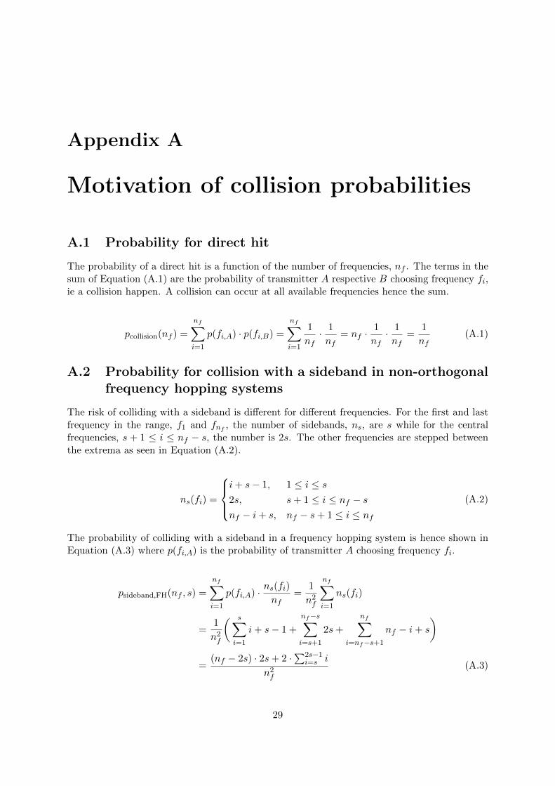
A.1 Probability for direct hit

The probability of a direct hit is a function of the number of frequencies, nf . The terms in thesum of Equation (A.1) are the probability of transmitter A respective B choosing frequency fi,ie a collision happen. A collision can occur at all available frequencies hence the sum.

pcollision(nf ) =

nf∑i=1

p(fi,A) · p(fi,B) =

nf∑i=1

1

nf· 1

nf= nf ·

1

nf· 1

nf=

1

nf(A.1)

A.2 Probability for collision with a sideband in non-orthogonalfrequency hopping systems

The risk of colliding with a sideband is different for different frequencies. For the first and lastfrequency in the range, f1 and fnf

, the number of sidebands, ns, are s while for the centralfrequencies, s + 1 ≤ i ≤ nf − s, the number is 2s. The other frequencies are stepped betweenthe extrema as seen in Equation (A.2).

ns(fi) =

i+ s− 1, 1 ≤ i ≤ s2s, s+ 1 ≤ i ≤ nf − snf − i+ s, nf − s+ 1 ≤ i ≤ nf

(A.2)

The probability of colliding with a sideband in a frequency hopping system is hence shown inEquation (A.3) where p(fi,A) is the probability of transmitter A choosing frequency fi.

psideband,FH(nf , s) =

nf∑i=1

p(fi,A) · ns(fi)nf

=1

n2f

nf∑i=1

ns(fi)

=1

n2f

( s∑i=1

i+ s− 1 +

nf−s∑i=s+1

2s+

nf∑i=nf−s+1

nf − i+ s

)

=(nf − 2s) · 2s+ 2 ·

∑2s−1i=s i

n2f(A.3)

29

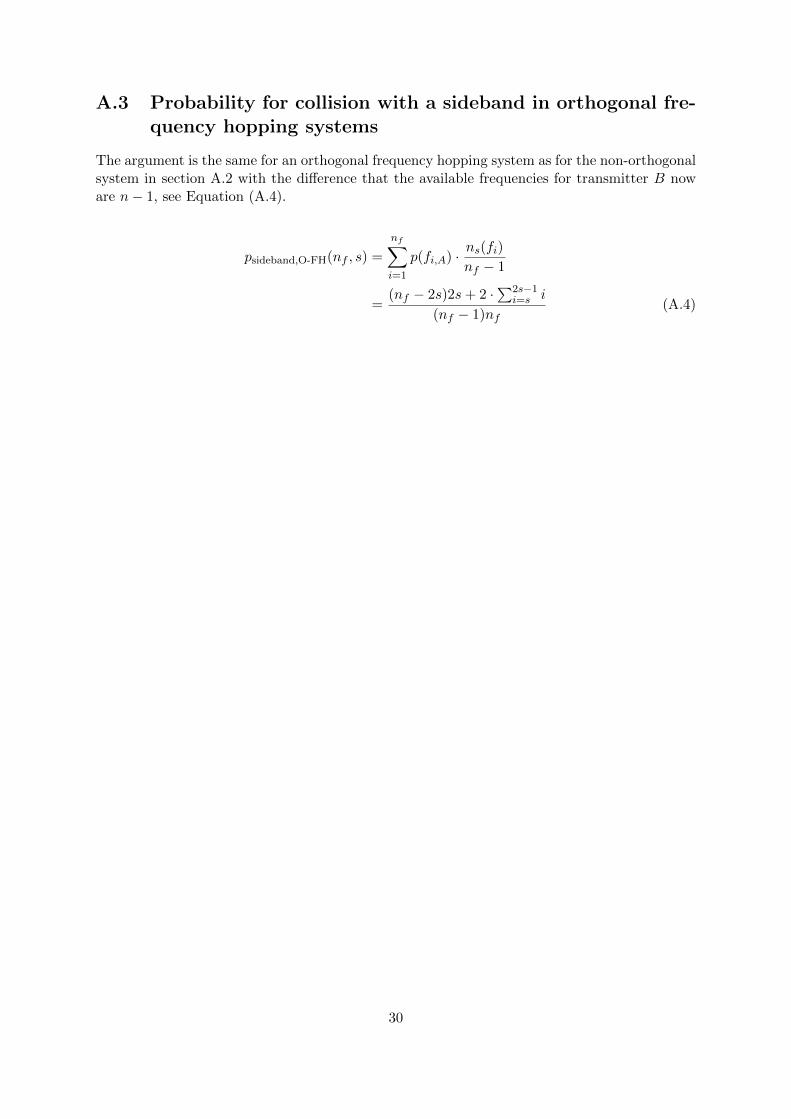
A.3 Probability for collision with a sideband in orthogonal fre-quency hopping systems

The argument is the same for an orthogonal frequency hopping system as for the non-orthogonalsystem in section A.2 with the difference that the available frequencies for transmitter B noware n− 1, see Equation (A.4).

psideband,O-FH(nf , s) =

nf∑i=1

p(fi,A) · ns(fi)nf − 1

=(nf − 2s)2s+ 2 ·

∑2s−1i=s i

(nf − 1)nf(A.4)

30