THE INTERCONNECTION PROBLEM: A TUTORIAL

David W. Hightower Bell Telephone Laboratories, Inc.

Introduction

This paper represents a fairly extensive survey of the literature on the interconnection problem. The topics covered are Pin Assignment, Layering, Ordering, Wire List Determination, Spanning Trees, Rectilinear Steiner Trees, and Wire Layout. In addition, several new ideas are pre­sented which could provide for better wire layout. Algo­rithms are presented in a way that makes them easy to understand, hence easy to discuss and apply. Formal state­ment of the algorithms can be found in the references cited.

Net List Determination

Starting Point The very beginning of the routing problem is a net list of some sort and a description of the circuit's geometry. In its most general form, the net list will be of the form shown in Figure 1.

The net list in Figure 1 denotes that some pin on com­ponent 1 (a dual in-line pack, for example) must connect to some pin on component 7. Furthermore, the gate which is selected on component 1 must be selected for net 10. In other words, nets 1 and 10 serve as inputs to the same logic

18 COMPUTER

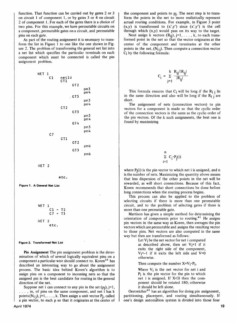
function. That function can be carried out by gates 2 or 3 on circuit 1 of component 1, or by gates 3 or 4 on circuit 2 of component 1. For each of the gates there is a choice of two pins. For this example, we have permutable circuits on a component, permutable gates on a circuit, and permutable pins on each gate.

As part of the routing assignment it is necessary to trans­form the list in Figure 1 to one like the one shown in Fig­ure 2. The problem of transforming the general net list into a net list which specifies the particular terminals on each component which must be connected is called the pin assignment problem.

NET 1 Cl netlü

CT1

CT2

C7 CT1

GT2

GT3

GT3

Glk

GT2

GT3

pn3 pnU

pn3 pnU

pn3 pnU

pn3 pnU

pnb

pnb

NET 2

etc.

Figure 1. A General Net List

NET 1 Cl - T2 C7 - T3

NET 2 e t c ,

Figure 2. Transformed Net List

Pin Assignment The pin assignment problem is the deter­mination of which of several logically equivalent pins on a component a particular wire should connect to. Koren33 has described an interesting way to go about the assignment process. The basic idea behind Koren's algorithm is to assign pins on a component to incoming nets so that the assigned pin is the best candidate for routing in the general direction of the net.

Suppose net i can connect to any pin in the set (pj), j=l, . . . , m, of pins on the same component, and net i has k points (Ni j ) , j=l , . . . , k. Then assign a unit vector Pj, called a pin vector, to each p so that it originates at the center of

April 1974

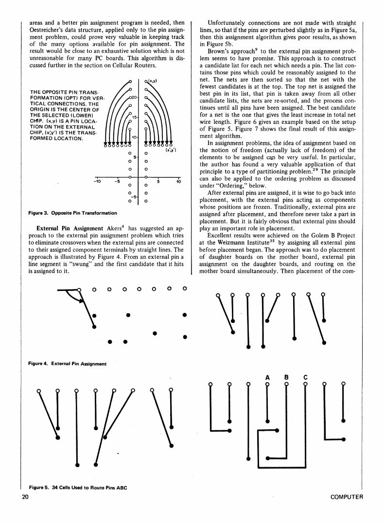
the component and points to pj. The next step is to trans­form the points in the net to more realistically represent actual routing conditions. For example, in Figure 3 point (x,y) is transformed to (x\y') since (x',y') is the cell through which (x,y) would pass on its way to the target.

Next assign k vectors (Ry), j=l, . . . , k, to each trans­formed point in the net so that the vector originates at the center of the component and terminates at the other points in the net, (Ni j). Then compute a connection vector Ci by the following formula:

k Rjj/IRyl Ci = Σ IR.-I

j=i y

This formula ensures that Ci will be long if the Rj j lie in the same direction and also will be long if the Rj j are short.

The assignment of nets (connection vectors) to pin vectors for a component is made so that the cyclic order of the connection vectors is the same as the cyclic order of the pin vectors. Of the k such assignments, the best one is found by maximizing

n Σ q-PjO)

i=l

where Pj(i) is the pin vector to which net i is assigned, and n is the number of nets. Maximizing the quantity above means that less dispersion of the other points in the net will be rewarded, as will short connections. Because of this fact, Koren recommends that short connections be done before long connections when the routing process begins.

This process can also be applied to the problem of selecting circuits if there is more than one permutable circuit, and to the problem of selecting gates if there is more than one permutable gate.

Mattison has given a simple method for determining the orientation of components prior to routing.41 He assigns pin vectors in the same way as Koren, then averages the pin vectors which are permutable and assigns the resulting vector to those pins. Net vectors are also computed in the same way but then are transformed as follows:

Let Vi be the net vector for net i computed as described above, then set Vj=l if it exits the right side of the component, Vi=-1 if it exits the left side and V=0 otherwise. Then compute the number X=Vi#Pi, Where Vj is the net vector for net i and Pi is the pin vector for the pin to which net i is assigned, If X<0 then the com­ponent should be rotated 180; otherwise it should be left alone.

Oestreicher45 has an algorithm for doing pin assignment, partitioning, placement, and routing simultaneously. If one's design automation system is divided into those four

19

areas and a better pin assignment program is needed, then Oestreicher's data structure, applied only to the pin assign­ment problem, could prove very valuable in keeping track of the many options available for pin assignment. The result would be close to an exhaustive solution which is not unreasonable for many PC boards. This algorithm is dis­cussed further in the section on Cellular Routers.

THE OPPOSITE PIN TRANS­FORMATION (OPT) FOR VER T ICAL CONNECTIONS. THE ORIGIN IS THE CENTER OF THE SELECTED (LOWER) CHIP. (x,y) IS A PIN LOCA­TION ON THE EXTERNAL CHIP, (χ',γ') IS THE TRANS­FORMED LOCATION.

o

o

-10 -5

-5

)Jx,y)

o

o

o

UV)

o

o

o

10

Figure 3. Opposite Pin Transformation

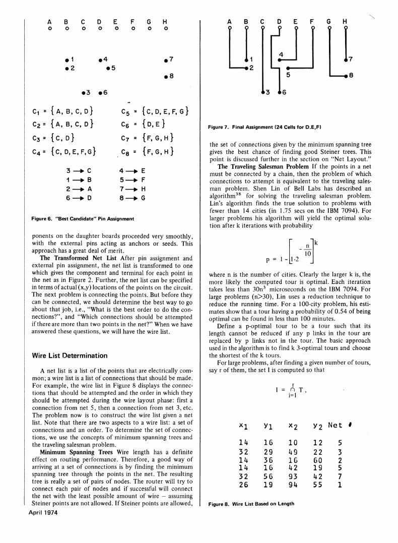
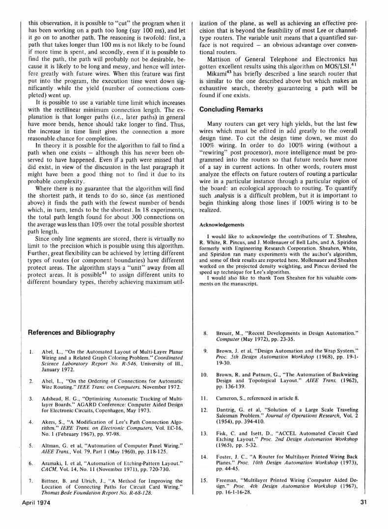
External Pin Assignment Akers4 has suggested an ap­proach to the external pin assignment problem which tries to eliminate crossovers when the external pins are connected to their assigned component terminals by straight lines. The approach is illustrated by Figure 4. From an external pin a line segment is "swung" and the first candidate that it hits is assigned to it.

• ·

Figure 4. External Pin Assignment

Figure 5. 34 Cells Used to Route Pins ABC

Unfortunately connections are not made with straight lines, so that if the pins are perturbed slightly as in Figure 5a, then this assignment algorithm gives poor results, as shown in Figure 5b.

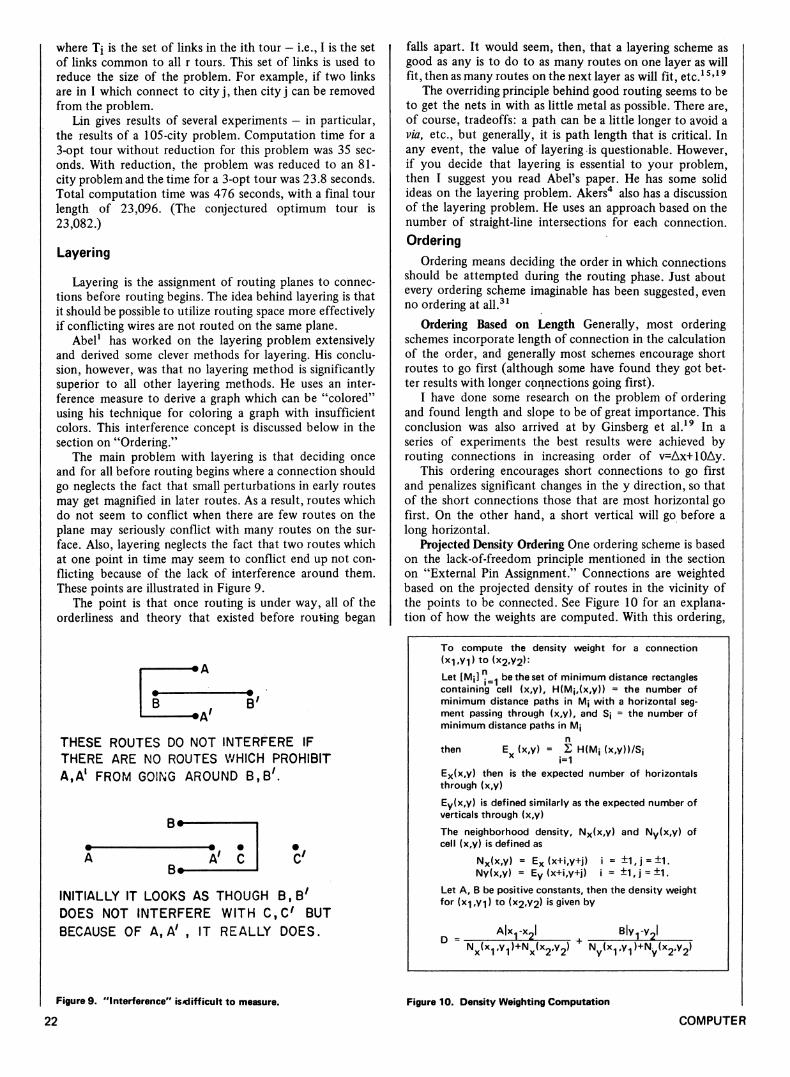
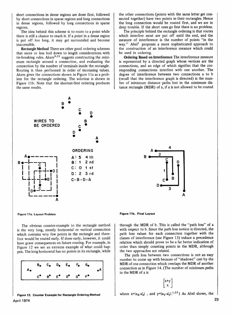
Brown's approach9 to the external pin assignment prob­lem seems to have promise. This approach is to construct a candidate list for each net which needs a pin. The list con­tains those pins which could be reasonably assigned to the net. The nets are then sorted so that the net with the fewest candidates is at the top. The top net is assigned the best pin in its list, that pin is taken away from all other candidate lists, the nets are re-sorted, and the process con­tinues until all pins have been assigned. The best candidate for a net is the one that gives the least increase in total net wire length. Figure 6 gives an example based on the setup of Figure 5. Figure 7 shows the final result of this assign­ment algorithm.

In assignment problems, the idea of assignment based on the notion of freedom (actually lack of freedom) of the elements to be assigned can be very useful. In particular, the author has found a very valuable application of that principle to a type of partitioning problem.29 The principle can also be applied to the ordering problem as discussed under 'Ordering," below.

After external pins are assigned, it is wise to go back into placement, with the external pins acting as components whose positions are frozen. Traditionally, external pins are assigned after placement, and therefore never take a part in placement. But it is fairly obvious that external pins should play an important role in placement.

Excellent results were achieved on the Golem B Project at the Weizmann Institute35 by assigning all external pins before placement began. The approach was to do placement of daughter boards on the mother board, external pin assignment on the daughter boards, and routing on the mother board simultaneously. Then placement of the com-

i i /

A o

B Q

c o

20 COMPUTER

A o

B o

• 1 • 2

C o

D o

E o

F o

G o

• 4 • 5

H o

• 7

• 8

• 3 · 6

c, ■ {A, B.C.D}

C2= {A , B, C, D}

c3= { C , D }

c4= {c, D.E.F.G}

3—► C 1 —► B 2—► A 6—► D

C5 = { c , D , E,F, G}

c6 - { D , E }

C7 ■ {F, G, H }

c8 = { F . G . H }

4—► E 5—+ F 7—► H 8—► G

Figure 6. "Best Candidate" Pin Assignment

ponents on the daughter boards proceeded very smoothly, with the external pins acting as anchors or seeds. This approach has a great deal of merit.

The Transformed Net List After pin assignment and external pin assignment, the net list is transformed to one which gives the component and terminal for each point in the net as in Figure 2. Further, the net list can be specified in terms of actual (x,y) locations of the points on the circuit. The next problem is connecting the points. But before they can be connected, we should determine the best way to go about that job, i.e., "What is the best order to do the con­nections?", and "Which connections should be attempted if there are more than two points in the net?" When we have answered these questions, we will have the wire list.

Wire List Determination

A net list is a list of the points that are electrically com­mon; a wire list is a list of connections that should be made. For example, the wire list in Figure 8 displays the connec­tions that should be attempted and the order in which they should be attempted during the wire layout phase: first a connection from net 5, then a connection from net 3, etc. The problem now is to construct the wire list given a net list. Note that there are two aspects to a wire list: a set of connections and an order. To determine the set of connec­tions, we use the concepts of minimum spanning trees and the traveling salesman problem.

Minimum Spanning Trees Wire length has a definite effect on routing performance. Therefore, a good way of arriving at a set of connections is by finding the minimum spanning tree through the points in the net. The resulting tree is really a set of pairs of nodes. The router will try to connect each pair of nodes and if successful will connect the net with the least possible amount of wire — assuming Steiner points are not allowed. If Steiner points are allowed,

April 1974

A o

B C O Ç> J E

Q F o

* 3 * 6

5

G H

Figure 7. Final Assignment (24 Cells for D.E,F)

the set of connections given by the minimum spanning tree gives the best chance of finding good Steiner trees. This point is discussed further in the section on "Net Layout."

The Traveling Salesman Problem If the points in a net must be connected by a chain, then the problem of which connections to attempt is equivalent to the traveling sales­man problem. Shen Lin of Bell Labs has described an algorithm38 for solving the traveling salesman problem. Lin's algorithm finds the true solution to problems with fewer than 14 cities (in 1.75 sees on the IBM 7094). For larger problems his algorithm will yield the optimal solu­tion after k iterations with probability

P = 1 1-2

n 10

where n is the number of cities. Clearly the larger k is, the more likely the computed tour is optimal. Each iteration takes less than 30n3 microseconds on the IBM 7094. For large problems (n>30), Lin uses a reduction technique to reduce the running time. For a 100-city problem, his esti­mates show that a tour having a probability of 0.54 of being optimal can be found in less than 100 minutes.

Define a p-optimal tour to be a tour such that its length cannot be reduced if any p links in the tour are replaced by p links not in the tour. The basic approach used in the algorithm is to find k 3-optimal tours and choose the shortest of the k tours.

For large problems, after finding a given number of tours, say r of them, the set I is computed so that

I = n T, i = l

11» 32 1U lh 32 26

16 29 36 16 56 19

X2 y2 Net #

10 i*9 16 U2 93 9U

12 22 60 19 1*2 55

5 3 2 5 7 1

Figure 8. Wire List Based on Length

where Tj is the set of links in the ith tour — i.e., I is the set of links common to all r tours. This set of links is used to reduce the size of the problem. For example, if two links are in I which connect to city j , then city j can be removed from the problem.

Lin gives results of several experiments — in particular, the results of a 105-city problem. Computation time for a 3-opt tour without reduction for this problem was 35 sec­onds. With reduction, the problem was reduced to an 81-city problem and the time for a 3-opt tour was 23.8 seconds. Total computation time was 476 seconds, with a final tour length of 23,096. (The conjectured optimum tour is 23,082.)

Layering

Layering is the assignment of routing planes to connec­tions before routing begins. The idea behind layering is that it should be possible to utilize routing space more effectively if conflicting wires are not routed on the same plane.

Abel1 has worked on the layering problem extensively and derived some clever methods for layering. His conclu­sion, however, was that no layering method is significantly superior to all other layering methods. He uses an inter­ference measure to derive a graph which can be "colored" using his technique for coloring a graph with insufficient colors. This interference concept is discussed below in the section on "Ordering."

The main problem with layering is that deciding once and for all before routing begins where a connection should go neglects the fact that small perturbations in early routes may get magnified in later routes. As a result, routes which do not seem to conflict when there are few routes on the plane may seriously conflict with many routes on the sur­face. Also, layering neglects the fact that two routes which at one point in time may seem to conflict end up not con­flicting because of the lack of interference around them. These points are illustrated in Figure 9.

The point is that once routing is under way, all of the orderliness and theory that existed before routing began

-•A

B;

THESE ROUTES DO NOT INTERFERE IF THERE ARE NO ROUTES WHICH PROHIBIT A,A1 FROM GOING AROUND Β,Β'.

B*-

B· -C

INITIALLY IT LOOKS AS THOUGH Β,Β' DOES NOT INTERFERE WITH C , C BUT BECAUSE OF A, A' , IT REALLY DOES.

Figure 9. "Interference" isdifficult to measure.

falls apart. It would seem, then, that a layering scheme as good as any is to do to as many routes on one layer as will fit, then as many routes on the next layer as will fit, etc.15'19

The overriding principle behind good routing seems to be to get the nets in with as little metal as possible. There are, of course, tradeoffs: a path can be a little longer to avoid a via, etc., but generally, it is path length that is critical. In any event, the value of layering is questionable. However, if you decide that layering is essential to your problem, then I suggest you read Abel's paper. He has some solid ideas on the layering problem. Akers4 also has a discussion of the layering problem. He uses an approach based on the number of straight-line intersections for each connection. Ordering

Ordering means deciding the order in which connections should be attempted during the routing phase. Just about every ordering scheme imaginable has been suggested, even no ordering at all.31

Ordering Based on Length Generally, most ordering schemes incorporate length of connection in the calculation of the order, and generally most schemes encourage short routes to go first (although some have found they got bet­ter results with longer connections going first).

I have done some research on the problem of ordering and found length and slope to be of great importance. This conclusion was also arrived at by Ginsberg et al.19 In a series of experiments the best results were achieved by routing connections in increasing order of ν=Δχ+10Δγ.

This ordering encourages short connections to go first and penalizes significant changes in the y direction, so that of the short connections those that are most horizontal go first. On the other hand, a short vertical will go before a long horizontal.

Projected Density Ordering One ordering scheme is based on the lack-of-freedom principle mentioned in the section on "External Pin Assignment." Connections are weighted based on the projected density of routes in the vicinity of the points to be connected. See Figure 10 for an explana­tion of how the weights are computed. With this ordering,

To compute the density weight for a connection (χ ΐ ,Υ ΐ ) to (x2,Y2):

Let [Mj ] . = 1 be the set of min imum distance rectangles containing cell (x,y), H(Mj,(x,y)) = the number of minimum distance paths in Mj wi th a horizontal seg­ment passing through (x,y), and Sj = the number of minimum distance paths in Mj

then E x ( x , y ) Σ H(Mj (x,y))/Sj i=1

Ex(x,y) then is the expected number of horizontals through (x,y)

Ev(x,y) is defined similarly as the expected number of verticals through (x,y)

The neighborhood density, Nx(x ,y) and Nv(x,y) of cell (x,y) is defined as

N x (x f y ) = E x (x+ i ,y+ j ) i = ± 1 , j = ± 1 . Ny(x,y) = E y (x+i,y+j) i = ± 1 f j = ± 1 .

Let A , B be positive constants, then the density weight for (x- | ,y i ) to (x2,Y2) i s given by

D = A|X1-X21

N x ( x 1 , y 1 ) + N x ( x 2 , y 2 )

B|y1-y2l N y ( x v V 1 ) + N v ( x 2 . V 2 )

Figure 10. Density Weighting Computation

22 COMPUTER

short connections in dense regions are done first, followed by short connections in sparse regions and long connections in dense regions, followed by long connections in sparse regions.

The idea behind this scheme is to route to a point while there is still a chance to reach it. If a point in a dense region is put off too long, it may get surrounded and become inaccessible.

Rectangle Method There are other good ordering schemes that more or less boil down to length considerations with tie-breaking rules. Akers4'31 suggests constructing the mini­mum rectangle around a connection, and evaluating the connection by the number of terminals inside the rectangle. Routing is then performed in order of increasing values. Akers gives the connections shown in Figure 1 la as a prob­lem for the rectangle ordering. The solution is shown in Figure l ib . Note that the shortest-first ordering produces the same results.

The obvious counter-example to the rectangle method is the very long, mostly horizontal or vertical connection which contains very few points in the rectangle and there­fore would be routed early. If done early, however, it could have grave consequences on future routing. For example, in Figure 12 we see an extreme example of what could hap­pen. The long horizontal has no points in its rectangle/while

B# C # D # E # F# G# A« *A

C # B# E # D# G# F#

Figure 12. Counter Example for Rectangle Ordering Method

April 1974

the other connections (points with the same letter get con­nected together) have two points in their rectangles. Hence the long connection would be routed first, and we are in deep trouble. If the short ones go first there is no problem.

The principle behind the rectangle ordering is that routes which interfere most are put off until the end, and the measure of interference is the number of points "in the way." Abel1 proposes a more sophisticated approach to the construction of an interference measure which could be used in ordering.

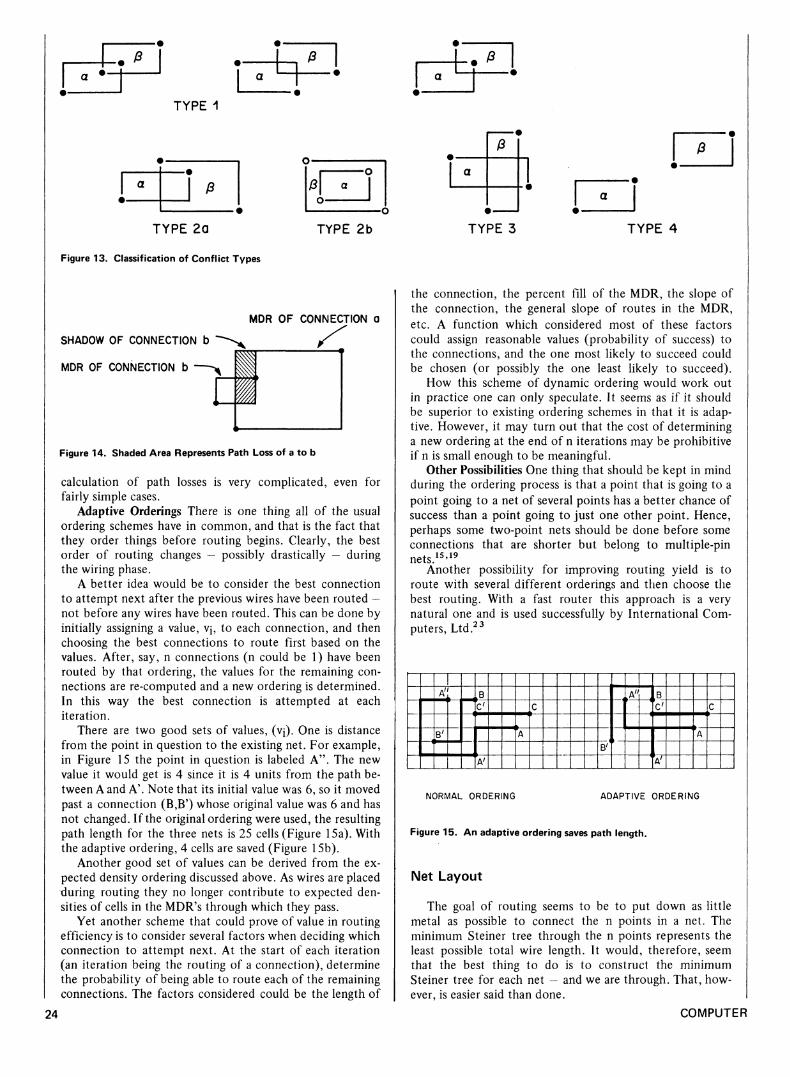
Ordering Based on Interference The interference measure is represented by a directed graph whose vertices are the connections, and an edge of which signifies that the cor­responding connections interfere with one another. The degree of interference between two connections a to b (recall that the interference graph is directed) is the num­ber of minimum distance paths lost in the minimum dis­tance rectangle (MDR) of a, if a is not allowed to be routed

through the MDR of b. This is called the "path loss" of a with respect to b. Since the path loss notion is directed, the path loss values for each connection together with the classes of interference (see Figure 13) induce a precedence relation which should prove to be a far better indication of order than simply counting points in the MDR, although the two approaches are related.

The path loss between two connections is not an easy number to come up with because of "shadows" cast by the MDR of one connection which overlaps the MDR of another connection as in Figure 14. (The number of minimum paths in the MDR of a is

m where x=|ax-a'x| , and y=|av-ay|.1'22) As Abel shows, the

B

WIRES TO BE ORDERED

A

D

C

c

D

B

A · , B r tT» « I ! ί i I

I I · C J

A

ORDERING A '· 5 4 th B: 1 2 nd C: 0 1 st D: 2 3 rd C - B - D - A

B *■

A ,— 4 2

( <

1'

U Wmam

>

ê l B

3

> I > 1

4

Figure 11a. Layout Problem Figure 11b. Final Layout

α ■

. ß • 1

• t-i ß I I α i — * ' · TYPE 1

• i 1—· I α I ß • 1

o -

Γ "O 1

a I G —o

TYPE 2a

Figure 13. Classification of Conflict Types

TYPE 2b

MDR OF CONNECTION a

SHADOW OF CONNECTION b

MDR OF CONNECTION b

Figure 14. Shaded Area Represents Path Loss of a to b

calculation of path losses is very complicated, even for fairly simple cases.

Adaptive Orderings There is one thing all of the usual ordering schemes have in common, and that is the fact that they order things before routing begins. Clearly, the best order of routing changes — possibly drastically — during the wiring phase.

A better idea would be to consider the best connection to attempt next after the previous wires have been routed — not before any wires have been routed. This can be done by initially assigning a value, vj, to each connection, and then choosing the best connections to route first based on the values. After, say, n connections (n could be 1) have been routed by that ordering, the values for the remaining con­nections are re-computed and a new ordering is determined. In this way the best connection is attempted at each iteration.

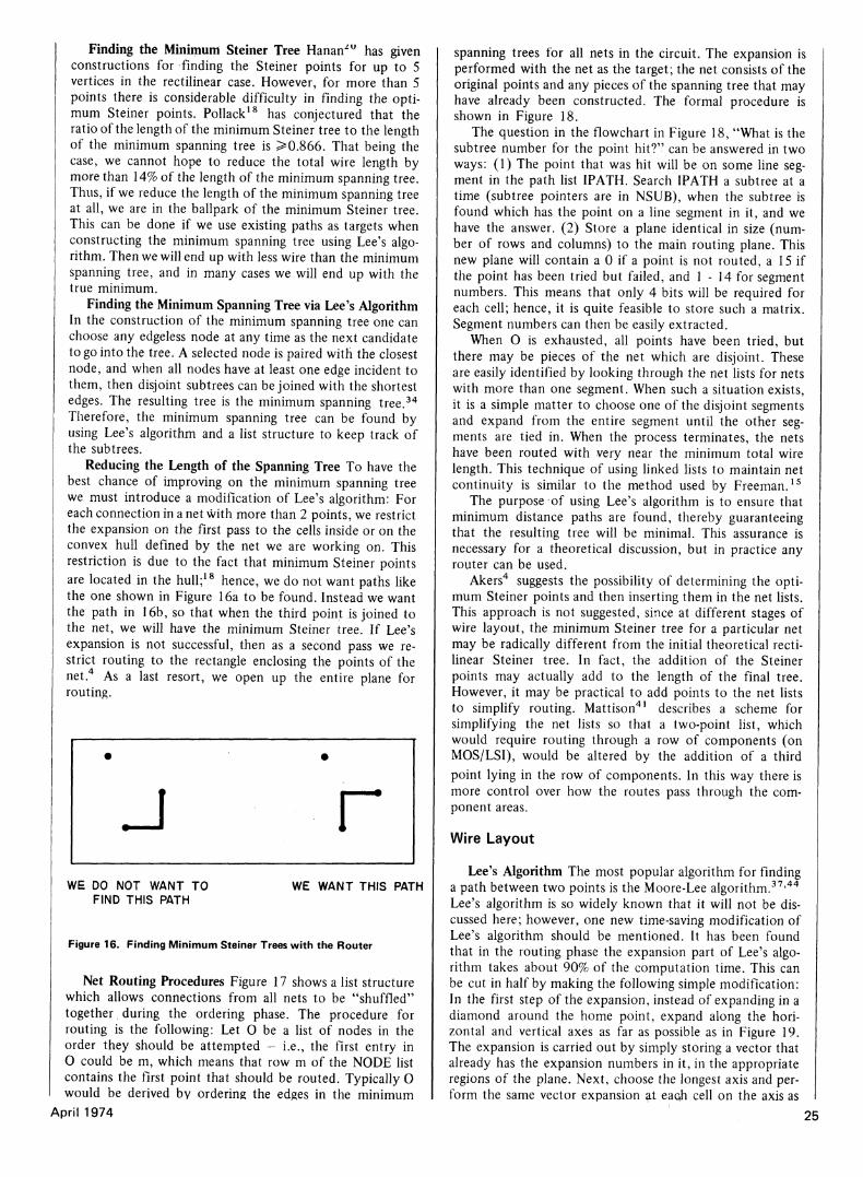
There are two good sets of values, (VJ). One is distance from the point in question to the existing net. For example, in Figure 15 the point in question is labeled A". The new value it would get is 4 since it is 4 units from the path be­tween A and A'. Note that its initial value was 6, so it moved past a connection (Β,Β') whose original value was 6 and has not changed. If the original ordering were used, the resulting path length for the three nets is 25 cells (Figure 15a). With the adaptive ordering, 4 cells are saved (Figure 15b).

Another good set of values can be derived from the ex­pected density ordering discussed above. As wires are placed during routing they no longer contribute to expected den­sities of cells in the MDR's through which they pass.

Yet another scheme that could prove of value in routing efficiency is to consider several factors when deciding which connection to attempt next. At the start of each iteration (an iteration being the routing of a connection), determine the probability of being able to route each of the remaining connections. The factors considered could be the length of

i — l · - · * I I α \—*

I ·

£ I • f-η

a I l··

• ' TYPE 3 TYPE 4

the connection, the percent fill of the MDR, the slope of the connection, the general slope of routes in the MDR, etc. A function which considered most of these factors could assign reasonable values (probability of success) to the connections, and the one most likely to succeed could be chosen (or possibly the one least likely to succeed).

How this scheme of dynamic ordering would work out in practice one can only speculate. It seems as if it should be superior to existing ordering schemes in that it is adap­tive. However, it may turn out that the cost of determining a new ordering at the end of n iterations may be prohibitive if n is small enough to be meaningful.

Other Possibilities One thing that should be kept in mind during the ordering process is that a point that is going to a point going to a net of several points has a better chance of success than a point going to just one other point. Hence, perhaps some two-point nets should be done before some connections that are shorter but belong to multiple-pin nets.15'19

Another possibility for improving routing yield is to route with several different orderings and then choose the best routing. With a fast router this approach is a very natural one and is used successfully by International Com­puters, Ltd.23

π~ 4 B'

,B C

A'

A

C

B'1

>A" lB c

A'

A

C

NORMAL ORDERING ADAPTIVE ORDERING

24

Figure 15. An adaptive ordering saves path length.

Net Layout

The goal of routing seems to be to put down as little metal as possible to connect the n points in a net. The minimum Steiner tree through the n points represents the least possible total wire length. It would, therefore, seem that the best thing to do is to construct the minimum Steiner tree for each net — and we are through. That, how­ever, is easier said than done.

COMPUTER

Finding the Minimum Steiner Tree Hanan2U has given constructions for finding the Steiner points for up to 5 vertices in the rectilinear case. However, for more than 5 points there is considerable difficulty in finding the opti­mum Steiner points. Pollack18 has conjectured that the ratio of the length of the minimum Steiner tree to the length of the minimum spanning tree is >0.866. That being the case, we cannot hope to reduce the total wire length by more than 14% of the length of the minimum spanning tree. Thus, if we reduce the length of the minimum spanning tree at all, we are in the ballpark of the minimum Steiner tree. This can be done if we use existing paths as targets when constructing the minimum spanning tree using Lee's algo­rithm. Then we will end up with less wire than the minimum spanning tree, and in many cases we will end up with the true minimum.

Finding the Minimum Spanning Tree via Lee's Algorithm In the construction of the minimum spanning tree one can choose any edgeless node at any time as the next candidate to go into the tree. A selected node is paired with the closest node, and when all nodes have at least one edge incident to them, then disjoint subtrees can be joined with the shortest edges. The. resulting tree is the minimum spanning tree.34

Therefore, the minimum spanning tree can be found by using Lee's algorithm and a list structure to keep track of the subtrees.

Reducing the Length of the Spanning Tree To have the best chance of improving on the minimum spanning tree we must introduce a modification of Lee's algorithm: For each connection in a net with more than 2 points, we restrict the expansion on the first pass to the cells inside or on the convex hull defined by the net we are working on. This restriction is due to the fact that minimum Steiner points are located in the hull;18 hence, we do not want paths like the one shown in Figure 16a to be found. Instead we want the path in 16b, so that when the third point is joined to the net, we will have the minimum Steiner tree. If Lee's expansion is not successful, then as a second pass we re­strict routing to the rectangle enclosing the points of the net.4 As a last resort, we open up the entire plane for routing.

J Γ WE DO NOT WANT TO WE WANT THIS PATH

FIND THIS PATH

Figure 16. Finding Minimum Steiner Trees with the Router

Net Routing Procedures Figure 17 shows a list structure which allows connections from all nets to be "shuffled" together during the ordering phase. The procedure for routing is the following: Let O be a list of nodes in the order they should be attempted - i.e., the first entry in 0 could be m, which means that row m of the NODE list contains the first point that should be routed. Typically O

I would be derived by ordering the edges in the minimum April 1974

spanning trees for all nets in the circuit. The expansion is performed with the net as the target; the net consists of the original points and any pieces of the spanning tree that may have already been constructed. The formal procedure is shown in Figure 18.

The question in the flowchart in Figure 18, "What is the subtree number for the point hit?" can be answered in two ways: (1) The point that was hit will be on some line seg­ment in the path list IPATH. Search IPATH a subtree at a time (subtree pointers are in NSUB), when the subtree is found which has the point on a line segment in it, and we have the answer. (2) Store a plane identical in size (num­ber of rows and columns) to the main routing plane. This new plane will contain a 0 if a point is not routed, a 15 if the point has been tried but failed, and 1 - 14 for segment numbers. This means that only 4 bits will be required for each cell; hence, it is quite feasible to store such a matrix. Segment numbers can then be easily extracted.

When O is exhausted, all points have been tried, but there may be pieces of the net which are disjoint. These are easily identified by looking through the net lists for nets with more than one segment. When such a situation exists, it is a simple matter to choose one of the disjoint segments and expand from the entire segment until the other seg­ments are tied in. When the process terminates, the nets have been routed with very near the minimum total wire length. This technique of using linked lists to maintain net continuity is similar to the method used by Freeman.15

The purpose of using Lee's algorithm is to ensure that minimum distance paths are found, thereby guaranteeing that the resulting tree will be minimal. This assurance is necessary for a theoretical discussion, but in practice any router can be used.

Akers4 suggests the possibility of determining the opti­mum Steiner points and then inserting them in the net lists. This approach is not suggested, since at different stages of wire layout, the minimum Steiner tree for a particular net may be radically different from the initial theoretical recti­linear Steiner tree. In fact, the addition of the Steiner points may actually add to the length of the final tree. However, it may be practical to add points to the net lists to simplify routing. Mattison41 describes a scheme for simplifying the net lists so that a two-point list, which would require routing through a row of components (on MOS/LSI), would be altered by the addition of a third point lying in the row of components. In this way there is more control over how the routes pass through the com­ponent areas.

Wire Layout

Lee's Algorithm The most popular algorithm for finding a path between two points is the Moore-Lee algorithm.37,44

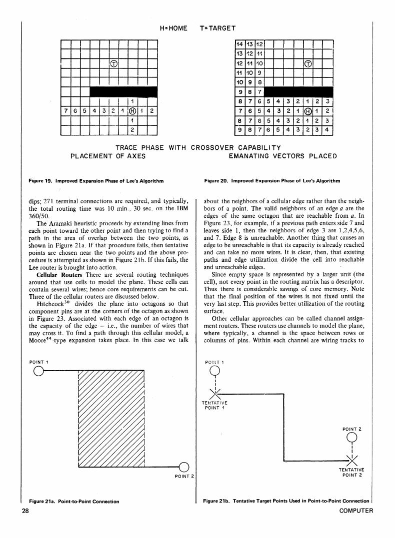
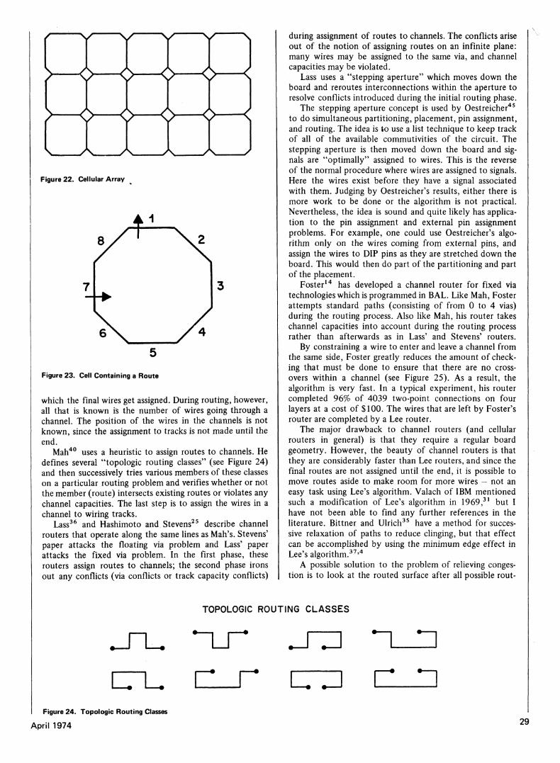
Lee's algorithm is so widely known that it will not be dis­cussed here; however, one new time-saving modification of Lee's algorithm should be mentioned. It has been found that in the routing phase the expansion part of Lee's algo­rithm takes about 90% of the computation time. This can be cut in half by making the following simple modification: In the first step of the expansion, instead of expanding in a diamond around the home point, expand along the hori­zontal and vertical axes as far as possible as in Figure 19. The expansion is carried out by simply storing a vector that already has the expansion numbers in it, in the appropriate regions of the plane. Next, choose the longest axis and per­form the same vector expansion ai eaqh cell on the axis as

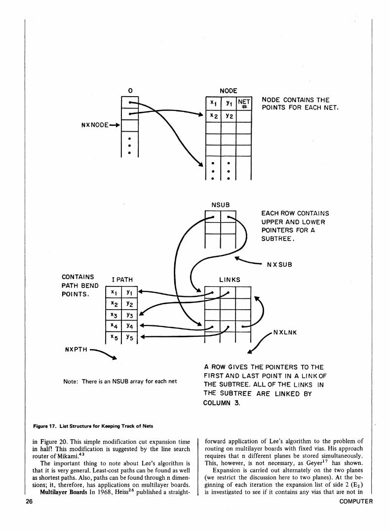
NODE

NXNODE·

P *2

• •

1 ·

V1

Y2

• e •

NET I NODE CONTAINS THE POINTS FOR EACH NET.

NSUB

CONTAINS PATH BEND POINTS.

I PATH

Γ**-*2 x3 x4

x5

~*ϊΊ y z

V3

V4

ys I NXPTH

Note: There is an NSUB array for each net

EACH ROW CONTAINS UPPER AND LOWER POINTERS FOR A SUBTREE.

NXSUB

Figure 17. List Structure for Keeping Track of Nets

in Figure 20. This simple modification cut expansion time in half! This modification is suggested by the line search router of Mikami.43

The important thing to note about Lee's algorithm is that it is very general. Least-cost paths can be found as well as shortest paths. Also, paths can be found through n dimen­sions; it, therefore, has applications on multilayer boards.

Multilayer Boards In 1968, Heiss26 published a straight-26

NXLNK

A ROW GIVES THE POINTERS TO THE FIRST AND LAST POINT IN A LINKOF THE SUBTREE. ALL OF THE LINKS IN THE SUBTREE ARE LINKED BY COLUMN 3.

forward application of Lee's algorithm to the problem of routing on multilayer boards with fixed vias. His approach requires that n different planes be stored simultaneously. This, however, is not necessary, as Geyer17 has shown.

Expansion is carried out alternately on the two planes (we restrict the discussion here to two planes). At the be­ginning of each iteration the expansion list of side 2 (E2) is investigated to see if it contains any vias that are not in

COMPUTER

NXNODE NXSU3t NXLNK

NXPTH=1 LINKS=0

GET THE NEXT MEMBERl

OF NODE USINGO

NO MORE NXSUB >2 YES

NO

( ST0P )

LINKS (NXLNK,1) = NXPTH

PUT PATH IN I PATH FROM NXPTH TO

IEND

LINKS (NXLNK,2); IEND

NXLNK=NXLNK+1 NXNODE=

NXNODE + 1 NXPTH=IEND + 1

EXPAND

WHAT IS THE SUBTREE NUMBER OF THE POINT

HIT(NT2)

l=0

NT2= NXSUB

NSUB(NXSUB,*) = NXLNK

NXSUB=NXSUBH

• -4

I RTF1 V - ^

> 0

v

LINKS (NXLNK,3) = NSUB(NT2,1) NSUB(NT2 ,1) =

NXLNK

h( *\ 3

NXSUB, NSUB depends on which net is being expanded

Figure 18. Routing Flow Chart

the expansion list of side 1 (Ei). If so, those points are moved into E! and then each point.in Εχ is expanded. (Expansion of a point means writing the next value in that point's neighboring cells; expansion of a set of points is defined naturally.) After E! is expanded, the points that were hit during the expansion replace the old points in E!. Then E! is investigated to see if it contains vias that are not in E2 ; if so, they are moved into E2, and E2 is expanded. etc.

This technique allows a path to cross between the two layers as many times as is necessary; however, Heiss has a bookkeeping method for avoiding unnecessary changes of layers. He also suggests that revising the trace part of the algorithm to change directions wherever possible will save

April 1974

NTREE=NXSUB-1 NXSUB=1

EXPAND FROM SUBTREE NXSUB

NT1 =NXSUB NT2 = HIT TREE

LINKS(NSUB(NT2,2),3)= NSUB(NT1,1) NSUB(NT1,1)=

NXLNK

space, since the resulting stairstep paths may be converted to diagonal paths when the routing is completed. (On the other hand, some people have found that diagonal paths cause problems.31)

Heuristics Coupled with Lee's Heuristics have been described6'14 which speed up routing by trying several standard type paths first. If these fail, then the full power of Lee's algorithm is brought into play. Foster's router14

is discussed below in the section on Cellular Routers. Aramaki6 found that such a heuristic can typically do

90% of the connections, and that Lee's can do most of the remainder. For most experiments, the time spent in the heuristic was about 50% of the total routing time. His experiments were carried out on a 2-sided board with 14

H=HOME T=TAR6ET

©

©

ρτ 13

12

11

10

9

8

7

8

I 9

^ 12

11

10

9

8

7

6

7 8

12

11

10

9

8

7

6

5

6 7

©

5

4

5 6

4

3

4 5

3

2

3 4

2

1

2 3

1

® 1 2

2

1

2 3

3] 2 !

3 4

TRACE PHASE V/ITH CROSSOVER CAPABILITY PLACEMENT OF AXES EMANATING VECTORS PLACED

Figure 19. Improved Expansion Phase of Lee's Algorithm

dips; 271 terminal connections are required, and typically, the total routing time was 10 min., 30 sec. on the IBM 360/50.

The Aramaki heuristic proceeds by extending lines from each point toward the other point and then trying to find a path in the area of overlap between the two points, as shown in Figure 21a. If that procedure fails, then tentative points are chosen near the two points and the above pro­cedure is attempted as shown in Figure 21b. If this fails, the Lee router is brought into action.

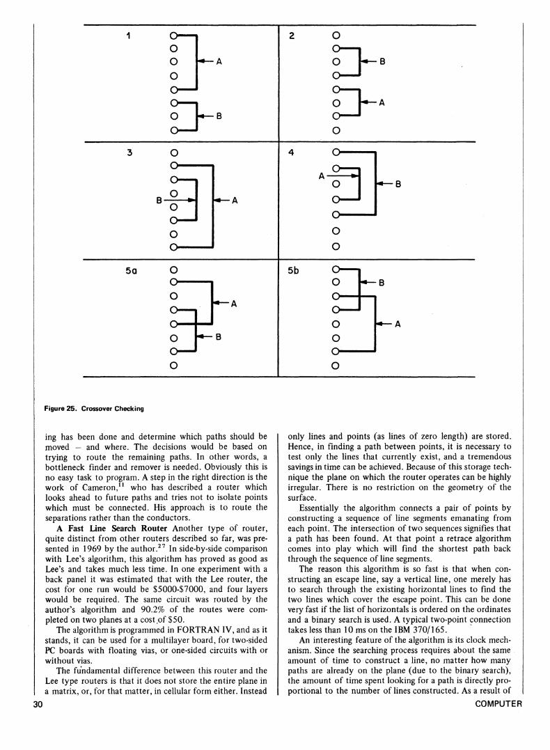
Cellular Routers There are several routing techniques around that use cells to model the plane. These cells can contain several wires; hence core requirements can be cut. Three of the cellular routers are discussed below.

Hitchcock30 divides the plane into octagons so that component pins are at the corners of the octagon as shown in Figure 23. Associated with each edge of an octagon is the capacity of the edge — i.e., the number of wires that may cross it. To find a path through this cellular model, a Moore44-type expansion takes place. In this case we talk

POINT 1

POINT 2

Figure 21a. Point-to-Point Connection

Figure 20. Improved Expansion Phase of Lee's Algorithm

about the neighbors of a cellular edge rather than the neigh­bors of a point. The valid neighbors of an edge a are the edges of the same octagon that are reachable from a. In Figure 23, for example, if a previous path enters side 7 and leaves side 1, then the neighbors of edge 3 are 1,2,4,5,6, and 7. Edge 8 is unreachable. Another thing that causes an edge to be unreachable is that its capacity is already reached and can take no more wires. It is clear, then, that existing paths and edge utilization divide the cell into reachable and unreachable edges.

Since empty space is represented by a larger unit (the cell), not every point in the routing matrix has a descriptor. Thus there is considerable savings of core memory. Note that the final position of the wires is not fixed until the very last step. This provides better utilization of the routing surface.

Other cellular approaches can be called channel assign­ment routers. These routers use channels to model the plane, where typically, a channel is the space between rows or columns of pins. Within each channel are wiring tracks to

POINT 1

9 \l/

TENTATIVE POINT 1

POINT 2 9

28

TENTATIVE POINT 2

Figure 21b. Tentative Target Points Used in Point-to-Point Connection

COMPUTER

/ s/ v V V S

? <> <> <> Φ S

>—6—6—6—Φ—< \__^/\__y\ /\__A /

Figure 22. Cellular Array

Figure 23. Cell Containing a Route

which the final wires get assigned. During routing, however, all that is known is the number of wires going through a channel. The position of the wires in the channels is not known, since the assignment to tracks is not made until the end.

Mah40 uses a heuristic to assign routes to channels. He defines several "topologic routing classes" (see Figure 24) and then successively tries various members of these classes on a particular routing problem and verifies whether or not the member (route) intersects existing routes or violates any channel capacities. The last step is to assign the wires in a channel to wiring tracks.

Lass36 and Hashimoto and Stevens25 describe channel routers that operate along the same lines as Mali's. Stevens' paper attacks the floating via problem and Lass' paper attacks the fixed via problem. In the first phase, these routers assign routes to channels; the second phase irons out any conflicts (via conflicts or track capacity conflicts)

during assignment of routes to channels. The conflicts arise out of the notion of assigning routes on an infinite plane: many wires may be assigned to the same via, and channel capacities may be violated.

Lass uses a "stepping aperture" which moves down the board and reroutes interconnections within the aperture to resolve conflicts introduced during the initial routing phase.

The stepping aperture concept is used by Oestreicher45

to do simultaneous partitioning, placement, pin assignment, and routing. The idea is to use a list technique to keep track of all of the available commutivities of the circuit. The stepping aperture is then moved down the board and sig­nals are "optimally" assigned to wires. This is the reverse of the normal procedure where wires are assigned to signals. Here the wires exist before they have a signal associated with them. Judging by Oestreicher's results, either there is more work to be done or the algorithm is not practical. Nevertheless, the idea is sound and quite likely has applica­tion to the pin assignment and external pin assignment problems. For example, one could use Oestreicher's algo­rithm only on the wires coming from external pins, and assign the wires to DIP pins as they are stretched down the board. This would then do part of the partitioning and part of the placement.

Foster14 has developed a channel router for fixed via technologies which is programmed in BAL. Like Mah, Foster attempts standard paths (consisting of from 0 to 4 vias) during the routing process. Also like Mah, his router takes channel capacities into account during the routing process rather than afterwards as in Lass' and Stevens' routers.

By constraining a wire to enter and leave a channel from the same side, Foster greatly reduces the amount of check­ing that must be done to ensure that there are no cross­overs within a channel (see Figure 25). As a result, the algorithm is very fast. In a typical experiment, his router completed 96% of 4039 two-point connections on four layers at a cost of $100. The wires that are left by Foster's router are completed by a Lee router.

The major drawback to channel routers (and cellular routers in general) is that they require a regular board geometry. However, the beauty of channel routers is that they are considerably faster than Lee routers, and since the final routes are not assigned until the end, it is possible to move routes aside to make room for more wires — not an easy task using Lee's algorithm. Valach of IBM mentioned such a modification of Lee's algorithm in 1969,31 but I have not been able to find any further references in the literature. Bittner and Ulrich35 have a method for succes­sive relaxation of paths to reduce clinging, but that effect can be accomplished by using the minimum edge effect in Lee's algorithm.37'4

A possible solution to the problem of relieving conges­tion is to look at the routed surface after all possible rout-

TOPOLOGIC ROUTING CLASSES

~T3 ~LJ=\ cru ci_r trz\ r n

Figure 24. Topologic Routing Classes

April 1974

o o

o o

5a O O

B

B

O O

5b O O

O O O

Figure 25. Crossover Checking

ing has been done and determine which paths should be moved — and where. The decisions would be based on trying to route the remaining paths. In other words, a bottleneck finder and remover is needed. Obviously this is no easy task to program. A step in the right direction is the work of Cameron,11 who has described a router which looks ahead to future paths and tries not to isolate points which must be connected. His approach is to route the separations rather than the conductors.

A Fast Line Search Router Another type of router, quite distinct from other routers described so far, was pre­sented in 1969 by the author.27 In side-by-side comparison with Lee's algorithm, this algorithm has proved as good as Lee's and takes much less time. In one experiment with a back panel it was estimated that with the Lee router, the cost for one run would be $5000-$7000, and four layers would be required. The same circuit was routed by the author's algorithm and 90.2% of the routes were com­pleted on two planes at a cost .of $50.

The algorithm is programmed in FORTRAN IV, and as it stands, it can be used for a multilayer board, for two-sided PC boards with floating vias, or one-sided circuits with or without vias.

The fundamental difference between this router and the Lee type routers is that it does not store the entire plane in a matrix, or, for that matter, in cellular form either. Instead

30

only lines and points (as lines of zero length) are stored. Hence, in finding a path between points, it is necessary to test only the lines that currently exist, and a tremendous savings in time can be achieved. Because of this storage tech­nique the plane on which the router operates can be highly irregular. There is no restriction on the geometry of the surface.

Essentially the algorithm connects a pair of points by constructing a sequence of line segments emanating from each point. The intersection of two sequences signifies that a path has been found. At that point a retrace algorithm comes into play which will find the shortest path back through the sequence of line segments.

The reason this algorithm is so fast is that when con­structing an escape line, say a vertical line, one merely has to search through the existing horizontal lines to find the two lines which cover the escape point. This can be done very fast if the list of horizontals is ordered on the ordinates and a binary search is used. A typical two-point connection takes less than 10 ms on the IBM 370/165.

An interesting feature of the algorithm is its clock mech­anism. Since the searching process requires about the same amount of time to construct a line, no matter how many paths are already on the plane (due to the binary search), j the amount of time spent looking for a path is directly pro­portional to the number of lines constructed. As a result of I

COMPUTER

this observation, it is possible to "cut" the program when it has been working on a path too long (say 100 ms), and let it go on to another path. The reasoning is twofold: first, a path that takes longer than 100 ms is not likely to be found if more time is spent, and secondly, even if it is possible to find the path, the path will probably not be desirable, be­cause it is likely to be long and messy, and hence will inter­fere greatly with future wires. When this feature was first put into the program, the execution time went down sig­nificantly while the yield (number of connections com­pleted) went up.

It is possible to use a variable time limit which increases with the rectilinear minimum connection length. The ex­planation is that longer paths (i.e., later paths) in general have more bends, hence should take longer to find. Thus, the increase in time limit gives the connection a more reasonable chance for completion.

In theory it is possible for the algorithm to fail to find a path when one exists — although this has never been ob­served to have happened. Even if a path were missed that did exist, in view of the discussion in the last paragraph it might have been a good thing not to find it due to its probable complexity.

Where there is no guarantee that the algorithm will find the shortest path, it tends to do so, since (as mentioned above) it finds the path with the fewest number of bends which, in turn, tends to be the shortest. In 18 experiments, the total path length found for about 300 connections on the average was less than 10% over the total possible shortest path length.

Since only line segments are stored, there is virtually no limit to the precision which is possible using this algorithm. Further, great flexibility can be achieved by letting different types of routes (or component boundaries) have different protect areas. The algorithm stays a "unit" away from all protect areas. It is possible41 to assign different units to different boundary types, thereby achieving maximum util-

References and Bibliography

1. Abel, L., ' O n the Automated Layout of Multi-Layer Planar Wiring and a Related Graph Coloring Problem." Coordinated Science Laboratory Report No. R-546, University of 111., January 1972.

2. Abel, L., "On the Ordering of Connections for Automatic Wire Routing." IEEE Trans, on Computers. November 1972.

3. Adshead, H. G., 'Optimizing Automatic Tracking of Multi­layer Boards." AGARD Conference: Computer Aided Design for Electronic Circuits, Copenhagen, May 1973.

4. Akers, S., "A Modification of Lee's Path Connection Algo­rithm." IEEE Trans, on Electronic Computers, Vol. EC-16, No. 1 (February 1967), pp. 97-98.

5. Altman, G. et al, "Automation of Computer Panel Wiring." AIEE Trans., Vol. 79, Part 1 (May 1960), pp. 118-125.

6. Aramaki, I. et al, "Automation of Etching-Pattern Layout." CACM, Vol. 14, No. 11 (November 1971), pp. 720-730.

7. Bittner, B. and Ulrich, J., "A Method for Improving the Location of Connecting Paths for Circuit Card Wiring." Thomas Bede Foundation Report No. R-68-128.

ization of the plane, as well as achieving an effective pre­cision that is beyond the feasibility of most Lee or channel-type routers. The variable unit means that a quantified sur­face is not required — an obvious advantage over conven­tional routers.

Mattisori of General Telephone and Electronics has gotten excellent results using this algorithm on MOS/LSI.41

Mikami43 has briefly described a line search router that is similar to the one described above but which makes an exhaustive search, thereby guaranteeing a path will be found if one exists.

Concluding Remarks

Many routers can get very high yields, but the last few wires which must be edited in add greatly to the overall design time. To cut the design time down, we must do 100% wiring. In order to do 100% wiring (without a "rewiring" post processor), more intelligence must be pro­grammed into the routers so that future needs have more of a say in current actions. In other words, routers must analyze the effects on future routers of routing a particular wire in a particular instance through a particular region of the board: an ecological approach to routing. To quantify such analysis is a difficult problem, but it is important to begin thinking along those lines if 100% wiring is to be realized.

Acknowledgements

I would like to acknowledge the contributions of T. Sheahen, R. White, R. Pincus, and J. MoUenauer of Bell Labs, and A. Spiridon formerly with Engineering Research Corporation. Sheahen, White, and Spiridon ran many experiments with the aulhor's algorithm, and some of their results are reported here. MoUenauer and Sheahen worked on the projected density weighting, and Pincus devised the speed up technique for Lee's algorithm.

I would also like to thank Tom Sheahen for his valuable com­ments on the manuscript.

8. Breuer, M., "Recent Developments in Design Automation." Computer (May 1972), pp. 23-35.

9. Brown, J. et al, "Design Automation and the Wrap System." Proc. 5th Design Automation Workshop (1968), pp. 19-1-19-30.

10. Brown, R. and Putnam, G., "The Automation of Backwiring Design and Topological Layout." AIEE Trans. (1962), pp. 136-139.

11. Cameron, S., referenced in article 8.

12. Dantzig, G. et al, "Solution of a Large Scale Traveling Salesman Problem." Journal of Operations Research, Vol. 2 (1954), pp. 394-410.

13. Fisk, C. and Isett, D., "ACCEL Automated Circuit Card Etching Layout." Proc. 2nd Design Automation Workshop (1965), pp. 5-32.

14. Foster, J. C . "A Router for Multilayer Printed Wiring Back Planes." Proc. 10th Design Automation Workshop (1973), pp. 44-45.

15. Freeman, "Multilayer Printed Wiring Computer Aided De­sign." Proc. 4th Design Automation Workshop (1967), pp. 16-1-16-28.

April 1974

16. Freitag, H., "Design Automation for Large Scale Integration." IBM Watson Research Center, Yorktown Heights, N.Y. Pre­sented at the Western Electronic Showland Convention, August 22-26, 1966.

17. Geyer, J., "Connection Routing Algorithm for Printed Cir­cuit BoardsriEEETCT, Vol. C-20, January 1971.

18. Gilbert, E. and Pollak, H., "Steiner Minimal Trees." SIAM J. Math., Vol. 16 (1968), pp. 1-29.

19. Ginsberg, G. et al, "An Updated Multilayer Printed Wiring CAD Capability." Proc. 6th Design Automation Workshop (1969), pp. 145-154.

20. Hanan, M., "On Steiner's Problem with Rectilinear Distance." SIAM Journal of Applied Math., Vol. 14, No. 2 (March 1966), pp. 255-265.

21. Hanan, M. and Kurtzberg, J., "A Review of the Placement and Quadratic Assignment Problems." IBM Research Report No. RC-3046, April 1970.

22. Hanan, M. and Oden, P., "A Wiring Problem for Large Scale Integrated Circuits." IBM Research Report No. RC-1615, May 17, 1966.

23. Hardgrave, W., "On the Relationship Between the Traveling Salesman and Longest Path Problems." Bell System Mono­graph No. 4336.

24. Harvey, J., "Automated Board Layout." Proc. 9th Design Automation Workshop (1972), pp. 264-271.

25. Hashimoto, A. and Stevens, J., "Wire Routing by Optimizing Channel Assignment within Large Apertures." Proc. 6th Design Automation Workshop (1969), pp. 155-169.

26. Heiss, S., "A Path Connection Algorithm for Multi-layer Boards." Proc. 5th Design Automation Workshop (1968), pp. 6-1-6-14.

27. Hightower, D. W., "A Solution to Line Routing Problems on the Continuous Plane." Proc. 6th Design Automation Work­shop (1969), pp. 1-24.

28. Hightower, D. W., "Interconnection Techniques." Proc. 1972 International Seminar on Design Automation, ILTAM, Jerusalem, Israel.

29. Hightower, D. W. and Unger, B., "A Method for Rapid Testing of Beam Crossover Circuits." Proc. 9th Design Auto­mation Workshop (1972), pp. 144-156.

30. Hitchcock, R., "Cellular Wiring and the Cellular Modeling Technique." Proc. 6th Design Automation Workshop (1969), pp. 25-41.

31. "IEEE Circuits Standards Committee Meeting Minutes." Naval Postgraduate School, Monterey, Calif., May 8-9, 1969.

32. Kernighan, B. and Lin, S., "An Efficient Heuristic Procedure for Partitioning Graphs." Bell System Technical Journal, Vol. 49, No. 2, February 1970, pp. 291-307.

33. Koren, N., "Pin Assignment in Automated Printed Circuit Board Design." Proc. 9th Design Automation Workshop (1972), pp. 72-79.

34. Kruscal, J., "On the Shortest Spanning Subtree of a Graph and the Traveling Salesman Problem." Proc. American Mathematical Society, Vol. 7 (1956), pp. 48-50.

35. Lapidot, Z. Private Communication.

36. Lass, S., "Automated Printed Circuit Routing with a Stepping Aperture." CACM, Vol. 12, No. 5 (May 1969).

37. Lee, C , "An Algorithm, for Path Connections and its Applications."//?/? Trans. On Electronic Computers (Septem­ber 1961), pp. 346-365.

38. Lin, S., "Computer Solutions of the Traveling Salesman Problem." Bell System Technical Journal, Vol. 44 (1965), pp. 2245-2269.

39. Loberman, H. and Weinberger, A., "Formal Procedures for Connecting Terminals with a Minimum Total Wire Length." JACM, Vol. 4 (October 1957), pp. 428-437.

40. Mah, L. and Steinberg, L., "Topologic Class Routing for Printed Circuit Boards." Proc. 9th Design Automation Work­shop (1972), pp. 80-93.

41. Mattison, R., "A High Quality, Low Cost Router for MOS/ LSI." Proc. 9th Design Automation Workshop (1972), pp. 94-103.

42. Michle, W. "Link-Length Minimization in Networks." Journal of Operations Research, Vol. 6 (1958), pp. 232-243.

43. Mikami, K. and Tabushi, K., "A Computer Program for Optimal Routing of Printed Circuit Connectors." IFIPS Proc, pp. 1475-1478.

44. Moore, E., "Shortest Path Through a Maze." Harvard Uni­versity Press, Cambridge, Mass., Vol. 30 (1959), pp. 285-292.

45. Oestreicher, D., "Automatic Printed Circuit Board Design." University of Utah Computer Science Division, UTEC-CSc-72-119, June 1972.

46. Prim, R., "Shortest Connection Networks and Some General­izations." Bell System Technical Journal, Vol. 36 (Novem­ber 1957).

47. Ramamoorthy, C , "Analysis of Graphs by Connectivity Considerations." JA CM, Vol. 13 (April 1966), pp. 211-222.

48. Rose, N. et al, "Printed Wiring Board Layout by Computer." Electronics and Power (October 1971), pp. 376-379.

49. Breuer, M., Design Automation of Digital Systems, Vol. 1, Prentice-Hall (1972).*

1 David W. Hightower is with Bell Labs at jHolmdel, New Jersey. Since joining Bell Labs in 11966 he has been involved in many aspects of | design automation with most of his efforts de­moted to the routing problem.

At present he is developing a routing system for large printed wiring boards. An integral part

lof the system is a routing algorithm which he I presented at the 1969 Design Automation Workshop.

In 1972 Mr. Hightower was invited to speak at the International Scientific Research Conferences in Jerusalem, Israel, and the Inter­national Seminar on Design Automation at the Weizmann Institute, Rehovot, Israel.

Mr. Hightower received his BS in math in 1966 and his MS in applied math from Stevens Institute of Technology in 1968. He is a member of the ACM and SIGDA and is Vice Chairman of the latter organization. He is also a Session Chairman for the 1974 Design Automation Workshop and for the 1974 ACM conference.

32

Reprints of this article are available at $1.50 for the first copy and $0.50 for each additional copy. Send request and remittance to IEEE Computer Society, using the Multi-purpose Order Form. I

COMPUTER