Embed Size (px)
Citation preview
·· · · · · · · ·············
····· ·· ·· ·
· ·· ·· ·· ··
··
··
··
·············
··· ···· ··
··
··
··
········
····· ··
·· ··
·· ··
··
··
··
·········· ·· ··
·· ··
·· ··
··
··
··
··
Universität Stuttgart
The Influence of Joint Parameters on DynamicResponse of Structures
Master Thesisvon
Darong Jin
durchgeführt am
Institut für Angewandte und Experimentelle MechanikUniversität Stuttgart
Institutsleiter: Prof. Dr.-Ing. habil. L. GaulBetreuer: Dipl.-Ing. Sergey Bograd
May 2011

I hereby declare that I have written this work independently, yet not otherwise provided
for audit purposes, other than those specified sources or equipment used as well as a
letter or in a quotes such was characterized.
Stuttgart, May 23, 2011 Darong Jin
Contents
1. Introduction 11.1. Introduction and Motivation . . . . . . . . . . . . . . . . . . . . . . 1
1.2. Previous Work . . . . . . . . . . . . . . . . . . . . . . . . . . . . . . 3
1.3. Objectives and Tasks . . . . . . . . . . . . . . . . . . . . . . . . . . 4
2. Theory 52.1. Analytical Modal Analysis . . . . . . . . . . . . . . . . . . . . . . . 6
2.1.1. Spatial Model to Response Model . . . . . . . . . . . . . . . 7
2.1.2. Modal Model to Response Model . . . . . . . . . . . . . . . 10
2.2. Experimental Modal Analysis . . . . . . . . . . . . . . . . . . . . . 12
2.2.1. Experiment Process . . . . . . . . . . . . . . . . . . . . . . . 12
2.2.2. Modal Parameter Estimation Methods . . . . . . . . . . . . . 13
2.2.3. Universal File Format (UFF) . . . . . . . . . . . . . . . . . . 19
2.3. FE Simulation . . . . . . . . . . . . . . . . . . . . . . . . . . . . . . 19
3. Design the System 233.1. Criteria . . . . . . . . . . . . . . . . . . . . . . . . . . . . . . . . . 23
3.2. Design . . . . . . . . . . . . . . . . . . . . . . . . . . . . . . . . . . 24
3.2.1. Assumption . . . . . . . . . . . . . . . . . . . . . . . . . . . 24
3.2.2. Sturcture . . . . . . . . . . . . . . . . . . . . . . . . . . . . 24
3.2.3. Simulation . . . . . . . . . . . . . . . . . . . . . . . . . . . 24
4. Analytical approach 314.1. Analytical Data Sets Creation . . . . . . . . . . . . . . . . . . . . . . 31
4.1.1. Analytical Data Sets With SISO Modal Model . . . . . . . . 32
4.1.2. Analytical Data Sets With MIMO Modal Model . . . . . . . . 33
4.1.3. Analytical Data Sets With MIMO Spatial Model . . . . . . . 33
4.2. Investigation of Modal Parameter Estimation Methods . . . . . . . . 34
4.2.1. Pole Selecting Methods . . . . . . . . . . . . . . . . . . . . 35
4.2.2. Frequency Resolution . . . . . . . . . . . . . . . . . . . . . 39

iv Contents
4.2.3. Modal Parameter Estimation Methods . . . . . . . . . . . . . 41
5. Experiment and Simulation 455.1. Experiment . . . . . . . . . . . . . . . . . . . . . . . . . . . . . . . 45
5.1.1. Experimental System Description . . . . . . . . . . . . . . . 45
5.1.2. Experimental Procedure . . . . . . . . . . . . . . . . . . . . 49
5.1.3. Data Processing . . . . . . . . . . . . . . . . . . . . . . . . . 53
5.2. Simulation . . . . . . . . . . . . . . . . . . . . . . . . . . . . . . . . 58
5.2.1. Adjust Material Properties . . . . . . . . . . . . . . . . . . . 58
5.2.2. Thin Layer Method . . . . . . . . . . . . . . . . . . . . . . . 60
6. Conclusions and Recommendations 696.1. Conclusions . . . . . . . . . . . . . . . . . . . . . . . . . . . . . . . 69
6.2. Recommendations . . . . . . . . . . . . . . . . . . . . . . . . . . . . 70
A. Appendix 73A.1. MATLAB codes . . . . . . . . . . . . . . . . . . . . . . . . . . . . . 73
A.2. ANSYS codes . . . . . . . . . . . . . . . . . . . . . . . . . . . . . . 74
A.3. Blueprint . . . . . . . . . . . . . . . . . . . . . . . . . . . . . . . . 77
List of Figures 82
List of Tables 84
Bibliography 87

1. Introduction
1.1. Introduction and Motivation
Nowadays, the daily life cannot separate apart from the mechanical systems and struc-
tures of mechanical systems are getting more and more complicated and sophisticated.
As examples for structure with numerous joints are showed in figure 1.1. The struc-
tures tend to contain a giant numbers of joints in the system which are one of the most
important factors that influence the dynamic response of the system. Investigation of
the relationship between the joint characteristics and the dynamical properties of struc-
ture is important for a various fields of research and industry.
Figure 1.1.: Examples of mechanical systems for daily life with numerous joints
2 1. Introduction
The vibrations and noises produced by mechanical systems serve as an important
criterion for customers. During the traveling with automobiles or airplanes, the vi-
brations and the noises are big annoyance factors which make the journey tired and
unpleasant. These are both affected by the dynamic properties of joint especially the
damping property. Even though the eigenfrequencies and mode shapes can be pre-
dicted successfully by existing Finite Element Method (FEM) software. However, the
damping property is still cannot be determined accurately with commercial FEM soft-
ware since less attention has paid to this fields of study.
The damping property is related to the dissipated energy during the dynamic process.
The dissipated energy is the culprit for vibrations and noises which are harmful for
systems and cause the fracture of systems. It is critical to design and analysis the
vibrating structures with respect to damping properties, since the dynamic response of
structures and transmission of vibrations to the environment is closely depended on the
damping mechanisms.
One of the existing approaches for dynamic analysis of mechanical systems is the
Experimental Modal Analysis (EMA) which is an experimental method used to extract
structural dynamic properties in terms of its modal parameters such as eigenfrequncies,
damping ratio as well as mode shapes. The general steps of EMA are: first, acquire
Frequency Response Functions (FRF) in the form of Universal File Format (UFF)
from the impact hammer experiment or experiment with shaker; second, from these
measured FRFs, Modal Parameter Estimation (MPE) with several different methods is
carried out and the modal parameters can be obtained as results. There are numbers
of MPE methods and the details about these methods are discussed in section 2.2.2.
In the thesis, several analytical modal data sets are created to compare these methods
with the software X-Modal II which is developed by the Structural Dynamics Research
Laboratory of University of Cincinnati (UC-SDRL). The damping is very sensitive, as
a consequence, the accuracy of these estimated modal parameters is greatly affected
by the method applied along with the other factors mentioned in section 4.2.
In order to reduce product development periods and associated costs, nowadays,
the industry is changing from the traditional ways of design to the Computer Aided
Design (CAD), the Computer Aided Simulation and the Computer Aided Manufactur-
ing (CAM). This means that the dynamical properties of a structure can be predicted
by the computer simulations before the physical prototype is available. One of the
standard approaches that allow the prediction of the vibration behavior for mechanical
products is the Finite Element (FE) simulation. Figuring out the relations between the
joint characteristic and the dynamic properties is the basic task and fundamentals for
computer simulations. In last years, it has reached a significant improvement and ap-
1.2. Previous Work 3
plied successfully to the software to estimate the eigenfrequencies and mode shapes of
complicated structures. However, the prediction of damping properties of structure, in
other words, the dissipative properties still cannot be determined accurately[23].
Therefore, there is an urgent need to develop a strong reliable dynamic analysis tools
which provide understandings of the interrelation between the joint characteristics and
dynamic properties. The joint characteristics of the structure contain contact pressure
and the distribution etc; the dynamic properties of the structure include eigenfrequen-
cies and mode shapes as well as the damping properties.
1.2. Previous Work
To give a brief overview of the ongoing work, the previous works which have taken
place in the mentioned research fields will be outlined here.
ANGEL MOISES IGLESIAS [10] did an investigation of four modal parameter
estimation methods both in time domain and frequency domain with respect to the
damping ratio. After introducing these modal parameter estimation methods, he com-
pared the methods with Single Input Single Output (SISO) analytical data sets as well
as the experiment data sets in the form of Frequency Response Functions (FRF) or Im-
pulse Response Function (IRF). This work shows that the time domain methods result
in better estimation with analytical data sets.
ALLEMANG, BROWN, PHILLIPS,ADAMS, MAIA and SILVA [21] [19] [20] [17]
[1] [15] provide the fundamentals of analytical modal analysis and experimental modal
analysis. They also give relatively detail descriptions of the existing modal parameter
estimation methods. The advantages and disadvantages have been discussed. They
also provide the introduction about the software X-Modal II which is developed by
UC-SDRL which using different MPE methods to obtain the modal parameters.
Many works has been done in the research fields of joint modeling by BOGRAD,
SCHMIT and GAUL [23] [22] [9]. They summarized the works have been done and
provide the overview of joint modeling. Also from their works, the damping prop-
erties of system were considered as the combination of material damping and joint
patch damping. They provide the experimental determination of two kinds of damp-
ing properties. Several different possibilities to implement the described models into
the FEM have been investigated. One of these is to express the damping properties
in terms of imaginary parts of the complex stiffness matrix. From the result of sim-
ulation and experiment with U-shaped structure made by thin plate with one of the
implementation FEM (Thin layer methods), the existence of certain relations between
joint characteristics and dynamic properties of the structure can be noticed.
4 1. Introduction
1.3. Objectives and Tasks
The goal of the master thesis is to investigate the interrelation between different joint
characteristics and the dynamic properties (modal parameters) of the assembled struc-
ture. The first task is to design simple structures of system which can provide different
joint characteristics and fulfills certain criteria. The second problem is to investigate
the modal parameter estimation methods with respect to several analytical data sets
with low damping ratio. Then the investigation of the interrelation between different
joint characteristics and the dynamic properties with the data sets acquired from im-
pact hammer experiments is carried out. At last, the simulation with thin layer methods
applied with the parameters given was performed to verify the investigation made by
the previous chapters. The following outlines of the thesis are showed below.
In Chapter 2, the theories of the method and experiment were presented. For the ana-
lytical modal analysis, theories about modal model and spatial model are discussed; for
experimental modal analysis, the procedure for the experiment, the modal parameter
estimation methods and the brief knowledge of universal file format were summarized
and introduced; for the Finite Element simulation, the detail theories about the simula-
tion with the thin layer method and how it is related to ANSYS are provided.
In Chapter 3, the system with multiple joint characteristics was designed and man-
ufactured. The procedure to check whether the structure satisfies the criteria was pre-
sented.
In Chapter 4, here we created several analytical data sets with the MATLAB code
and used the data sets to investigate the modal parameter estimation methods with
respect to several factors, including pole selecting method; frequency resolution and
also different MPE methods applied.
In Chapter 5, here we talked the detail about the experiment and the simulation. In
the first part, we gave the detail description, the procedure and the important points
about the experiment, then the result was given, the data processing was operated and
the brief conclusion was made.
In Chapter 6, Summarization of the important points over the entire master thesis
was made, and then the recommendations for the further works were given.
In Appendix A the main part of MATLAB code to create the analytical model,
the ANSYS code to perform the simulation with thin layer element method and the
blueprints of the structures used in the thesis are given.
2. Theory
This chapter will show the detail theories which are related to the thesis, including
analytical and experimental modal analysis, modal parameter estimation methods, and
Finite Element simulation with thin layer elements method. For analytical modal anal-
ysis, the theories used to develop the analytical model data sets which will be used
in comparison with different modal parameter estimation methods are discussed. For
experimental modal analysis, the procedure applied to establish the experiment is in-
troduced. For modal parameter estimation methods, the brief introduction and summa-
rization of the theories of the MPE methods used in our data processing stage as well
as the knowledge about universal file format was presented. At last, theories related to
the simulation with thin layer method were discussed.
Assumptions [19] [20] for analytical modal analysis and experiment modal analysis
was presented as following.
• The structure must be a linear system which means the system must be repre-
sented by a set of linear, second order differential equations.
• The structure must be time invariant during the dynamic process. This implies
that the coefficients in the linear, second order differential equations are con-
stants with respect to time.
• The structure must be observable. This means that the system characteristics
describing the dynamic properties can be measured, in other words, there are
sufficient sensors to adequately describe the input-output characteristics of the
system. A linear system is observable if and only if the initial state can be deter-
mined from a finite interval of the output signals.
• The structure obeys Maxwell’s reciprocity theorem. This implies the following:
if one measures the frequency response function between points p and q by excit-
ing at p and measuring the response at q, the same frequency response function
will be measured by exciting at q and measuring the response at p which means
Hpq = Hqp.
6 2. Theory
2.1. Analytical Modal Analysis
There are three different presentations for analytical model for the dynamic system.
First one is the spatial model which is represented with the mass matrix, stiffness
matrix, and damping matrix. Second one is the modal model which requires the modal
parameters such as eigenfrequencies, mode shapes and damping ratios. The last one
is the response model in the forms of Frequency Response Function (FRF) or Impulse
Response Function (IRF). These models can represent the analytical Multi Input Multi
Output (MIMO) model.
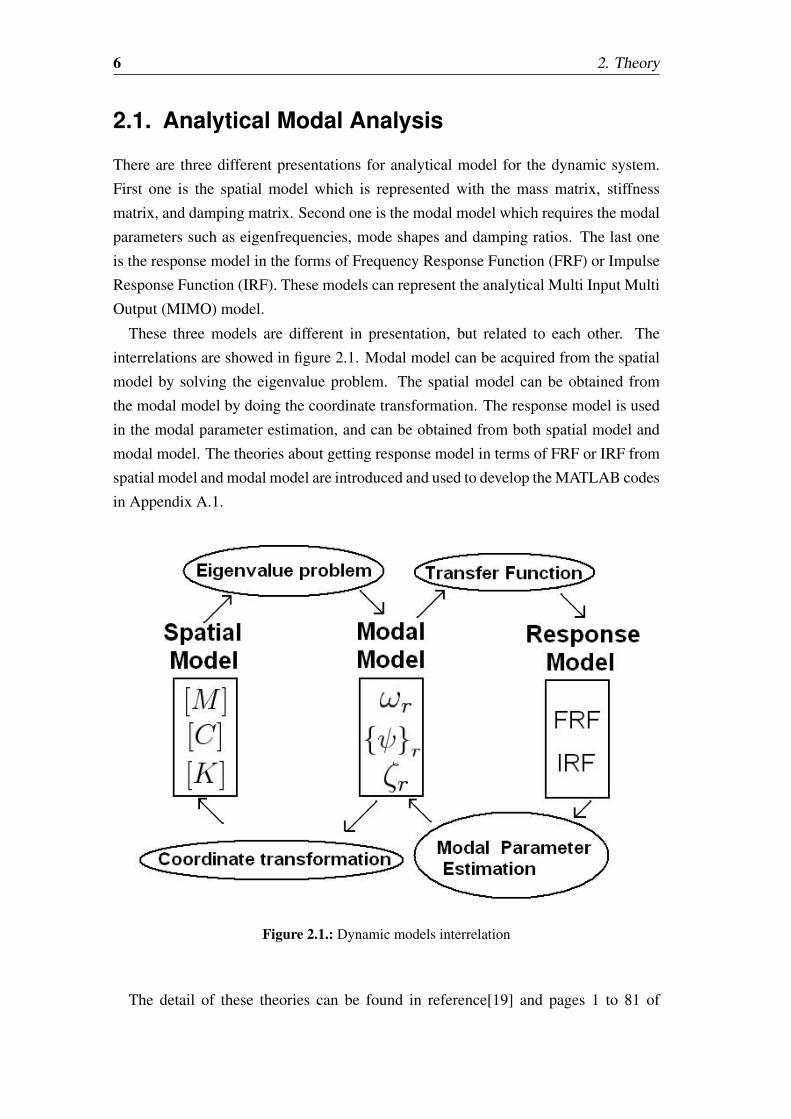
These three models are different in presentation, but related to each other. The
interrelations are showed in figure 2.1. Modal model can be acquired from the spatial
model by solving the eigenvalue problem. The spatial model can be obtained from
the modal model by doing the coordinate transformation. The response model is used
in the modal parameter estimation, and can be obtained from both spatial model and
modal model. The theories about getting response model in terms of FRF or IRF from
spatial model and modal model are introduced and used to develop the MATLAB codes
in Appendix A.1.
Figure 2.1.: Dynamic models interrelation
The detail of these theories can be found in reference[19] and pages 1 to 81 of
2.1. Analytical Modal Analysis 7
reference[15].
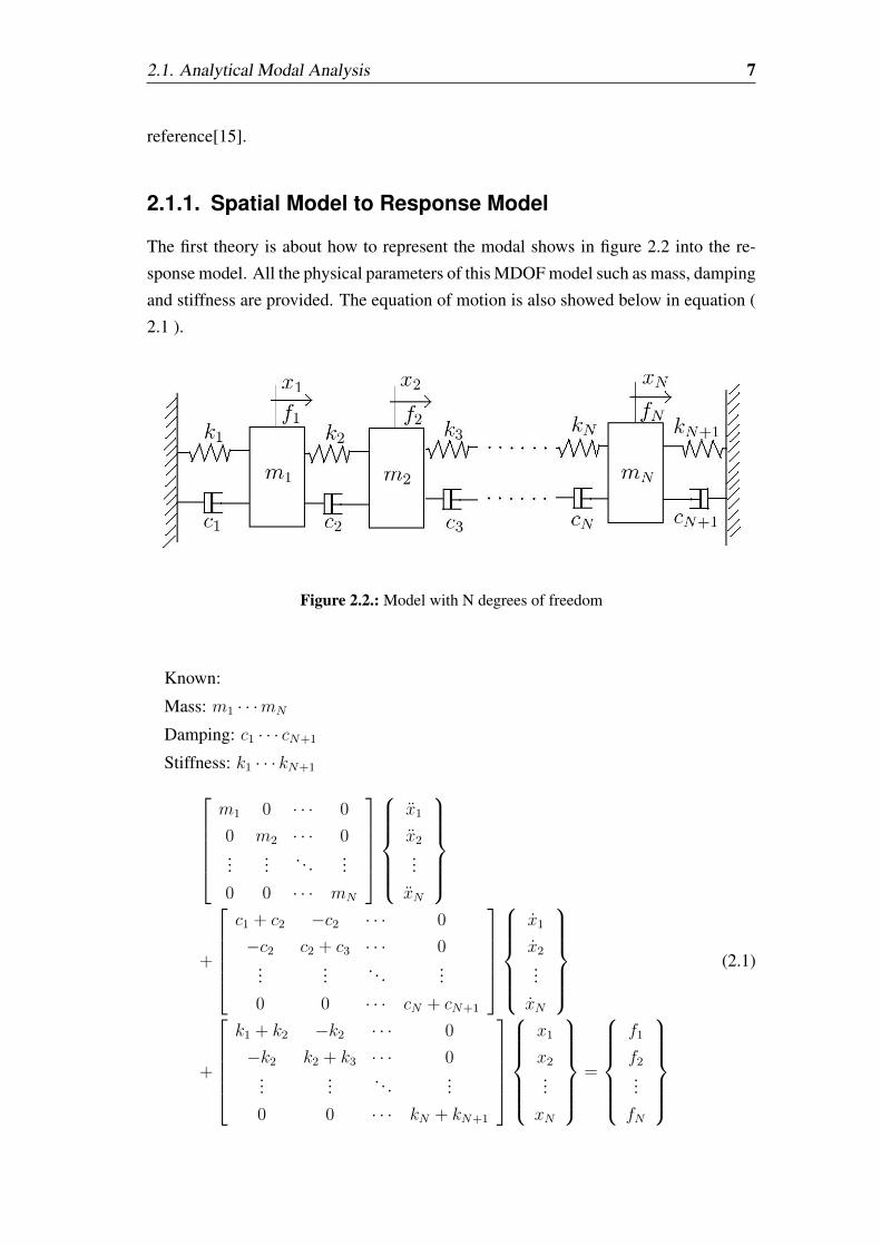
2.1.1. Spatial Model to Response Model
The first theory is about how to represent the modal shows in figure 2.2 into the re-
sponse model. All the physical parameters of this MDOF model such as mass, damping
and stiffness are provided. The equation of motion is also showed below in equation (
2.1 ).
Figure 2.2.: Model with N degrees of freedom
Known:
Mass: m1 · · ·mN
Damping: c1 · · · cN+1
Stiffness: k1 · · · kN+1m1 0 · · · 0
0 m2 · · · 0...
... . . . ...
0 0 · · · mN
x1
x2
...
xN
+
c1 + c2 −c2 · · · 0
−c2 c2 + c3 · · · 0...
... . . . ...
0 0 · · · cN + cN+1
x1
x2
...
xN
+
k1 + k2 −k2 · · · 0
−k2 k2 + k3 · · · 0...
... . . . ...
0 0 · · · kN + kN+1
x1
x2
...
xN
=
f1
f2
...
fN
(2.1)
8 2. Theory
This can be written in the short form of equation ( 2.2 ).
[M ] x+ [C] x+ [K] x = f (2.2)
Where [M ] is mass matrix, [C] is damping matrix, [K] is stiffness matrix, f is
input force.
When the damping matrix [C] is non-proportional, the equations ( 2.2 ) ofN−degree
freedom system cannot yield the eigenvectors which can diagonalize the damping ma-
trix. A technique can be used to solve this problem by reformulating the set of N
equations into set of 2N equations known as Hamilton‘s Canonical Equations [19].
Consequently, The reformulation must be applied for the general damping matrix [C].
The identity ( 2.3 ) will be take in consider.
[M ] x − [M ] x = 0 (2.3)
Combine equations ( 2.2 ) and ( 2.3 ) yield a new system of 2N equations.
[A] y+ [B] y =f
(2.4)
Where
[A] =
[[0] [M ]
[M ] [C]
][B] =
[− [M ] [0]
[0] [K]
]
y =
xx
y =
xx
f
=
0f
(2.5)
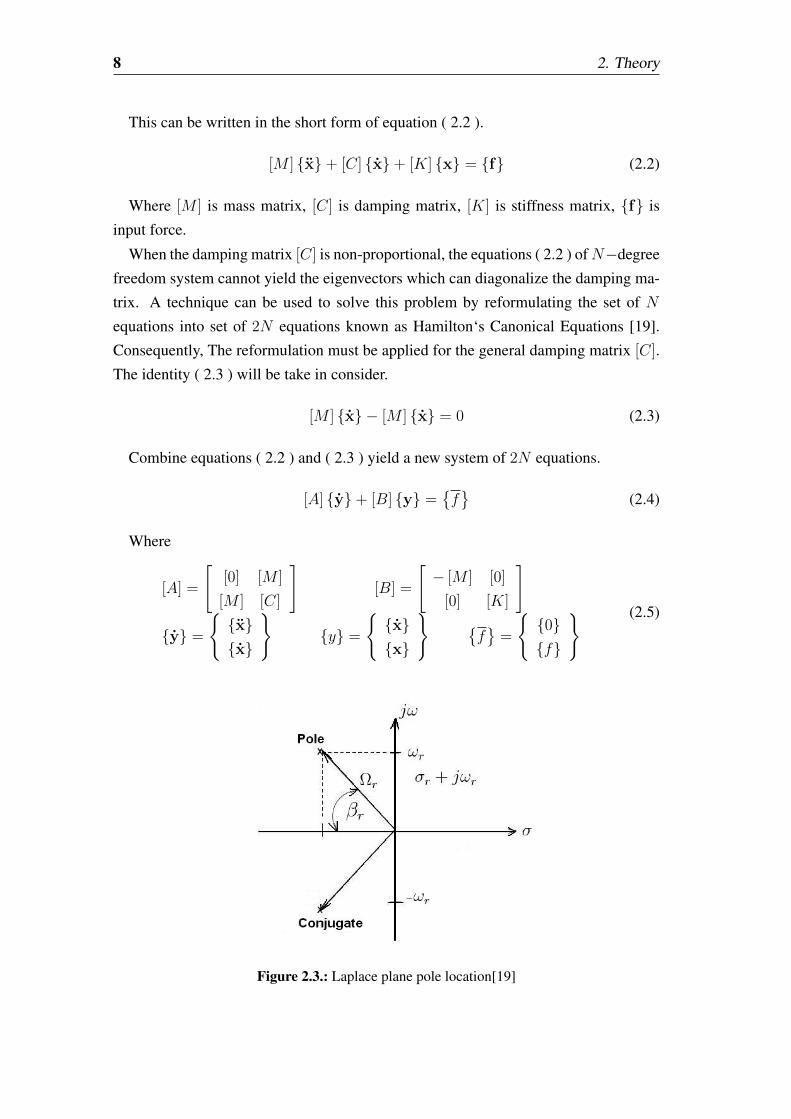
Figure 2.3.: Laplace plane pole location[19]
2.1. Analytical Modal Analysis 9
Note that all matrices in equation ( 2.4) are symmetric and this equation is now
in a classical eigenvalue solution form. For this method, after solving the eigenvalue
problem and obtaining the poles of the system, The eigenfrequencies and damping
ratios can be calculated using the equations ( 2.7 ) ( 2.8 ). The locations of ploes are
showed in the figure 2.3 and the notations used in the figure can be found following.
σr : damping coefficient
ωr : damped natural freqeuncy
Ωr : resonant (undamped natural frequency)
ζr = cos βr : damping factor (or percent of critical damping)
The pole λr cay be written as
λr = σr + jωr =(−ζr + j
√1− ζ2
r
)Ωr (2.6)
From the above relationship, the following equations can be derived. damping ratio:
ζr =−σr√ω2r + σ2
r
(2.7)
damped natural frequency:
fr =ωr2π
(2.8)
And for the 2N equation of system, we will use ϕ as the eigenvector. Notation
ψ is used for eigenvector of the original N equation system.
[ϕ] =[ϕ1 ϕ2 · · · ϕr · · · ϕ2N
](2.9)
[ϕ] =
[λ1 ψ1 λ2 ψ2 · · · λr ψr · · · λ2N ψ2N
ψ1 ψ2 · · · ψr · · · ψ2N
](2.10)
Modal A is used for the theoretical case of damped systems (non-proportional or
proportional), the modal A scaling factor is also the basis for the relationship between
the scaled modal vectors and the residues determined from the measured frequency
response functions. In general, for most experimental work, modal A is used as the
default scaling approach. Starting with the analytical definition of modal mass in 2N
space.
MAr = ϕTr
[[0] [M ]
[M ] [C]
]ϕr
=
λr ψrψr
T [[0] [M ]
[M ] [C]
]λr ψrψr
(2.11)
10 2. Theory
Multiplying Equation ( 2.11 ) out in terms of space yields:
MAr = λr ψTr [M ] ψr + λr ψTr [M ] ψr + ψTr [C] ψr= λrMr + λrMr + Cr = 2λrMr + Cr
(2.12)
Applying the SDOF relationship between the modal damping and modal mass,
Cr = −σrMr ⇒MAr = 2λrMr − 2σrMr
MAr = 2 (σr + jωr)Mr − 2σrMr = j2ωrMr
(2.13)
where MAr refers to modal A for mode r; Mr is modal mass for mode r. From
relationship between modal mass Mr and scaling factor Qr, The relationship between
MAr and Qr in Equation ( 2.14 ) can be obtained.
Mr =1
j2ωrQr
⇒ MAr =1
Qr
(2.14)
Then the residue Apqr is
Apqr = Qrψprψqr (2.15)
Finally, The Frequency Response Function (FRF) and Impulse Response Function
(IRF) with the relation in equantion ( 2.16 ) can be derived.
Hpq (ω) =N∑r=1
Apqr
jω−λr +A∗pqrjω−λ∗r
hpq (t) =N∑r=1
Apqreλrt + A∗pqre
λ∗rt
(2.16)
2.1.2. Modal Model to Response Model
The second theory is about how to represent the modal model into the response model.
All the modal parameters of this MDOF model such as eigenfrequencies, modal damp-
ing ratios and the mode shapes in the terms of eigenvectors are provided.
Known:
Eigenfrequency for mode r: ωr = 2πfr ;
Modal damping ration for mode r: ζr ;
Scaled eigenvector for mode r: ψr ;
Residue for response location p, reference location q, for mode r: Apq;
We know the transfer function of the multi degree of freedom system as
Hpq (s) =N∑r=1
Apqrs− λr
+A∗pqr
s− λ∗pqr(2.17)
whereHpq is transfer function for response location p, reference location q; N refers to
the number of modes; λr is rth system eigenvalue or system pole; s is Laplace domain
variable.
2.1. Analytical Modal Analysis 11
The Hpq (s) canbedefinedasHpq (s) = Xp(s)
Fq(s)(2.18)
Therefore
Xp (s) = Fq (s)N∑r=1
Apqrs− λr
+A∗pqr
s− λ∗pqr(2.19)
The impulse excitation force will be unity after the Laplace transformation. So we
can say Fq (s) = 1.
hpq (t) = L−1 Xp (s) = L−1
N∑r=1
Apqrs− λr
+A∗pqr
s− λ∗pqr=
N∑r=1
Apqreλrt + A∗pqre
λ∗rt
(2.20)
Where hpq (t) refers to impulse response funtion for response location p, reference
location q.
From the figure 2.3, the following equation can be drived.
λr = σr + jωr (2.21)
λr = σr − jωr (2.22)
Where σr refers to real part of the system pole, or damping for mode r.
And then, the equation as following is defined
Apqr =Rpqr
2j(2.23)
Using Euler‘s formula, equantion ( 2.20 ) becomes
hpq (t) =N∑r=1
Rpqr
2j
[e(σr+jωr)t − e(σr−jωr)t
]=
N∑r=1
Rpqreσrt (e
jωrt−e−jωrt)2j
=N∑r=1
Rpqreσrt sin (ωrt)
(2.24)
The residues can be obtained from the known mode shapes.
[A]r = Qr ψr ψTr ⇒ Apqr = Qrψprψqr (2.25)
whereQr is constant which is scaling factor. TheQr can be determined as following
Qr =1
2jωrMr
(2.26)
Equation ( 2.26 ) represents the relationship between modal mass and the scaling
involved between the residues and the modal vectors. Therefore, once the residue
information is found for mode r and some convenient form of modal vector scaling is
12 2. Theory
chosen for mode r, the scaling constant can be determined. Equation ( 2.26 ) can be
used to determine modal mass for mode r consistent with the modal vector scaling.
These theories discussed above are used to develop the MATLAB code which is used
to create several analytical data sets in the form of response model from both modal
model and spatial model to verify the modal parameter estimation methods. And this
part is also the fundamentals of experimental modal analysis.
2.2. Experimental Modal Analysis
Experimental modal analysis is an experimental approach to determine the modal pa-
rameters (eigenfrequencies, damping factors, modal vectors and modal scaling) of a
system under the assumptions established in the begging of the Chapter. The modal
parameters determined experimentally serve for future evaluations such as structural
modifications. Experimental modal analysis is used to explain dynamic problems such
as vibration or acoustic that is not obvious from the analytical models. It is important to
remember that most vibration and acoustic problems are a function of both the forcing
functions (or initial conditions) and the system characteristics described by the modal
parameters [20]. As a result, the experimental modal analysis can be summarized as
two steps: Experimental Data Acquisition and Data Processing.
The detail of the experimental modal analysis can be found in reference [15] and
reference [20]. Here the details about the theories related to experiment and modal
parameter estimation methods are presented.
2.2.1. Experiment Process
• Discretize structure and define nodes
• Either use roving sensor(s) (and fixed actuator(s)) Or roving actuator(s) (and
fixed sensor(s))
• Excite the structure using impact hammer or shaker as actuator
• Measurement of all input and output signals
• Calculate frequency response function (FRF)
• Perfrom modal parameter estimation from acquired FRF signals
2.2. Experimental Modal Analysis 13
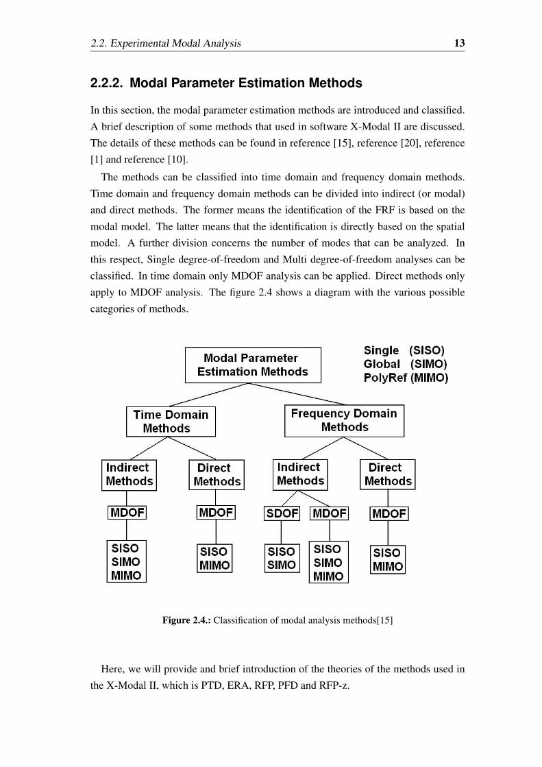
2.2.2. Modal Parameter Estimation Methods
In this section, the modal parameter estimation methods are introduced and classified.
A brief description of some methods that used in software X-Modal II are discussed.
The details of these methods can be found in reference [15], reference [20], reference
[1] and reference [10].
The methods can be classified into time domain and frequency domain methods.
Time domain and frequency domain methods can be divided into indirect (or modal)
and direct methods. The former means the identification of the FRF is based on the
modal model. The latter means that the identification is directly based on the spatial
model. A further division concerns the number of modes that can be analyzed. In
this respect, Single degree-of-freedom and Multi degree-of-freedom analyses can be
classified. In time domain only MDOF analysis can be applied. Direct methods only
apply to MDOF analysis. The figure 2.4 shows a diagram with the various possible
categories of methods.
Figure 2.4.: Classification of modal analysis methods[15]
Here, we will provide and brief introduction of the theories of the methods used in
the X-Modal II, which is PTD, ERA, RFP, PFD and RFP-z.
14 2. Theory
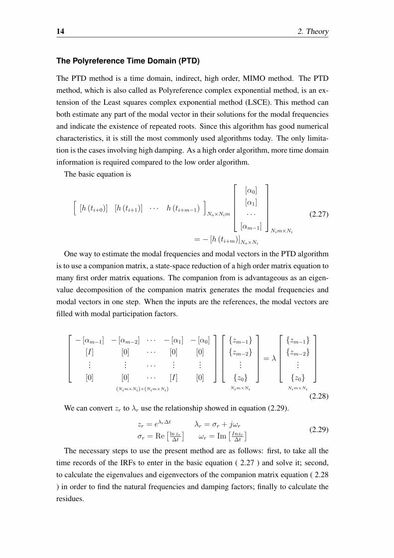
The Polyreference Time Domain (PTD)
The PTD method is a time domain, indirect, high order, MIMO method. The PTD
method, which is also called as Polyreference complex exponential method, is an ex-
tension of the Least squares complex exponential method (LSCE). This method can
both estimate any part of the modal vector in their solutions for the modal frequencies
and indicate the existence of repeated roots. Since this algorithm has good numerical
characteristics, it is still the most commonly used algorithms today. The only limita-
tion is the cases involving high damping. As a high order algorithm, more time domain
information is required compared to the low order algorithm.
The basic equation is
[[h (ti+0)] [h (ti+1)] · · · h (ti+m−1)
]No×Nim
[α0]
[α1]
· · ·[αm−1]
Nim×Ni
= − [h (ti+m)]No×Ni
(2.27)
One way to estimate the modal frequencies and modal vectors in the PTD algorithm
is to use a companion matrix, a state-space reduction of a high order matrix equation to
many first order matrix equations. The companion from is advantageous as an eigen-
value decomposition of the companion matrix generates the modal frequencies and
modal vectors in one step. When the inputs are the references, the modal vectors are
filled with modal participation factors.
− [αm−1] − [αm−2] · · · − [α1] − [α0]
[I] [0] · · · [0] [0]...
... · · · ......
[0] [0] · · · [I] [0]
(Nim×Ni)×(Nim×Ni)
zm−1zm−2
...
z0
Nim×Ni
= λ
zm−1zm−2
...
z0
Nim×Ni
(2.28)
We can convert zr to λr use the relationship showed in equation (2.29).
zr = eλr∆t λr = σr + jωr
σr = Re[
ln zr∆t
]ωr = Im
[Inzr∆t
] (2.29)
The necessary steps to use the present method are as follows: first, to take all the
time records of the IRFs to enter in the basic equation ( 2.27 ) and solve it; second,
to calculate the eigenvalues and eigenvectors of the companion matrix equation ( 2.28
) in order to find the natural frequencies and damping factors; finally to calculate the
residues.
2.2. Experimental Modal Analysis 15
This method can determine the multiple roots or closely spaced modes of a struc-
ture. The time required for the analysis is reduced and the accuracy in the results
increased. It has also shown some difficulties in analyzing satisfactorily structures
with high damping.
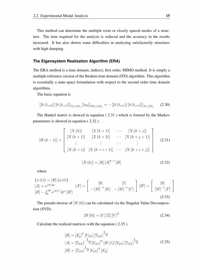
The Eigensystem Realization Algorithm (ERA)
The ERA method is a time domain, indirect, first order, MIMO method. It is simply a
multiple reference version of the Ibrahim time domain (ITD) algorithm. This algorithm
is essentially a state-space formulation with respect to the second order time domain
algorithms.
The basic equation is
[[h (ti+0)] [h (ti+1)]]Ni×2No[[α0]]2N0×2No
= − [[h (ti+1)] [h (ti+2)]]Ni×2No(2.30)
The Hankel matrix is showed in equation ( 2.31 ) which is formed by the Markov
parameters is showed in equation ( 2.32 ).
[H (k − 1)] =
[X (k)] [X (k + 1)] · · · [X (k + j)]
[X (k + 1)] [X (k + 2)] · · · [X (k + j + 1)]...
... · · · ...
[X (k + i)] [X (k + i+ 1)] · · · [X (k + i+ j)]
(2.31)
[X (k)] = [R] [A]k−1 [B] (2.32)
where
x (t) = [R] u (t)[A] = e[A′]∆t
[B]−∫ ∆t
0e[A′]τ ′dτ ′ [B′]
[A′] =
[[0] [I]
− [M ]−1 [K] − [M ]−1 [C]
][B′] =
[[0]
[M ]−1 [F ]
](2.33)
The pseudo-inverse of [H (0)] can be calculated via the Singular Value Decomposi-
tion (SVD).
[H (0)] = [U ] [Σ] [V ]T (2.34)
Calculate the realized matrices with the equation ( 2.35 ).
[R] = [Ep]T [U2N ] [Σ2N ]
1/2
[A] = [Σ2N ]−1/2 [U2N ]T [H (1)] [V2N ] [Σ2N ]
1/2
[B] = [Σ2N ]1/2 [V2N ]T [Eq]
(2.35)
16 2. Theory
where [Ep]T =
[[I] [0] · · · [0]
][Eq] =
[I]
[0]...
[0]
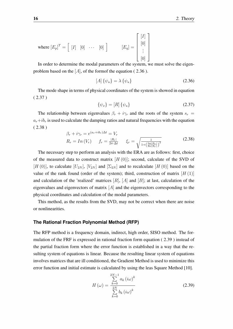
In order to determine the modal parameters of the system, we must solve the eigen-
problem based on the [A], of the formof the equation ( 2.36 ).
[A] ψu = λ ψu (2.36)
The mode shape in terms of physical coordinates of the system is showed in equation
( 2.37 )
ψx = [R] ψu (2.37)
The relationship between eigenvalues βr + iγr and the roots of the system sr =
ar+ibr is used to calculate the damping ratios and natural frequencies with the equation
( 2.38 )βr + iγr = e(ar+ibr)∆t = Vr
Rr = In (Vr) fr = |Rr|2π·∆t ξr =
√1
1+( Im(Rr)Re(Rr)
)2
(2.38)
The necessary step to perform an analysis with the ERA are as follows: first, choice
of the measured data to construct matrix [H (0)]; second, calculate of the SVD of
[H (0)], to calculate [U2N ], [V2N ] and [Σ2N ] and to recalculate [H (0)] based on the
value of the rank found (order of the system); third, construction of matrix [H (1)]
and calculation of the ’realized’ matrices [R], [A] and [B]; at last, calculation of the
eigenvalues and eigenvectors of matrix [A] and the eigenvectors corresponding to the
physical coordinates and calculation of the modal parameters.
This method, as the results from the SVD, may not be correct when there are noise
or nonlinearities.
The Rational Fraction Polynomial Method (RFP)
The RFP method is a frequency domain, indirect, high order, SISO method. The for-
mulation of the FRF is expressed in rational fraction form equation ( 2.39 ) instead of
the partial fraction form where the error function is established in a way that the re-
sulting system of equations is linear. Because the resulting linear system of equations
involves matrices that are ill conditioned, the Gradient Method is used to minimize this
error function and initial estimate is calculated by using the leas Square Method [10].
H (ω) =
2N−1∑k=0
ak (iω)k
2N∑k=0
bk (iω)k(2.39)
2.2. Experimental Modal Analysis 17
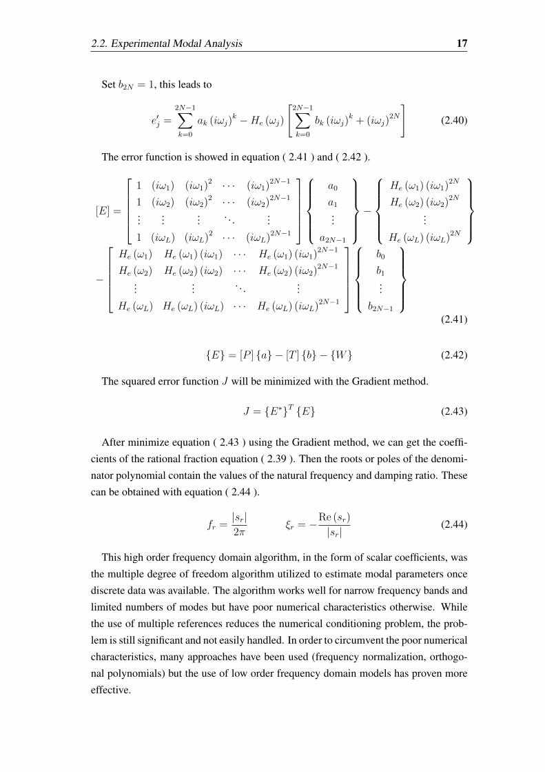
Set b2N = 1, this leads to
e′j =2N−1∑k=0
ak (iωj)k −He (ωj)
[2N−1∑k=0
bk (iωj)k + (iωj)
2N
](2.40)
The error function is showed in equation ( 2.41 ) and ( 2.42 ).
[E] =
1 (iω1) (iω1)2 · · · (iω1)2N−1
1 (iω2) (iω2)2 · · · (iω2)2N−1
......
... . . . ...
1 (iωL) (iωL)2 · · · (iωL)2N−1
a0
a1
...
a2N−1
−
He (ω1) (iω1)2N
He (ω2) (iω2)2N
...
He (ωL) (iωL)2N
−
He (ω1) He (ω1) (iω1) · · · He (ω1) (iω1)2N−1
He (ω2) He (ω2) (iω2) · · · He (ω2) (iω2)2N−1
...... . . . ...
He (ωL) He (ωL) (iωL) · · · He (ωL) (iωL)2N−1
b0
b1
...
b2N−1
(2.41)
E = [P ] a − [T ] b − W (2.42)
The squared error function J will be minimized with the Gradient method.
J = E∗T E (2.43)
After minimize equation ( 2.43 ) using the Gradient method, we can get the coeffi-
cients of the rational fraction equation ( 2.39 ). Then the roots or poles of the denomi-
nator polynomial contain the values of the natural frequency and damping ratio. These
can be obtained with equation ( 2.44 ).
fr =|sr|2π
ξr = −Re (sr)
|sr|(2.44)
This high order frequency domain algorithm, in the form of scalar coefficients, was
the multiple degree of freedom algorithm utilized to estimate modal parameters once
discrete data was available. The algorithm works well for narrow frequency bands and
limited numbers of modes but have poor numerical characteristics otherwise. While
the use of multiple references reduces the numerical conditioning problem, the prob-
lem is still significant and not easily handled. In order to circumvent the poor numerical
characteristics, many approaches have been used (frequency normalization, orthogo-
nal polynomials) but the use of low order frequency domain models has proven more
effective.
18 2. Theory
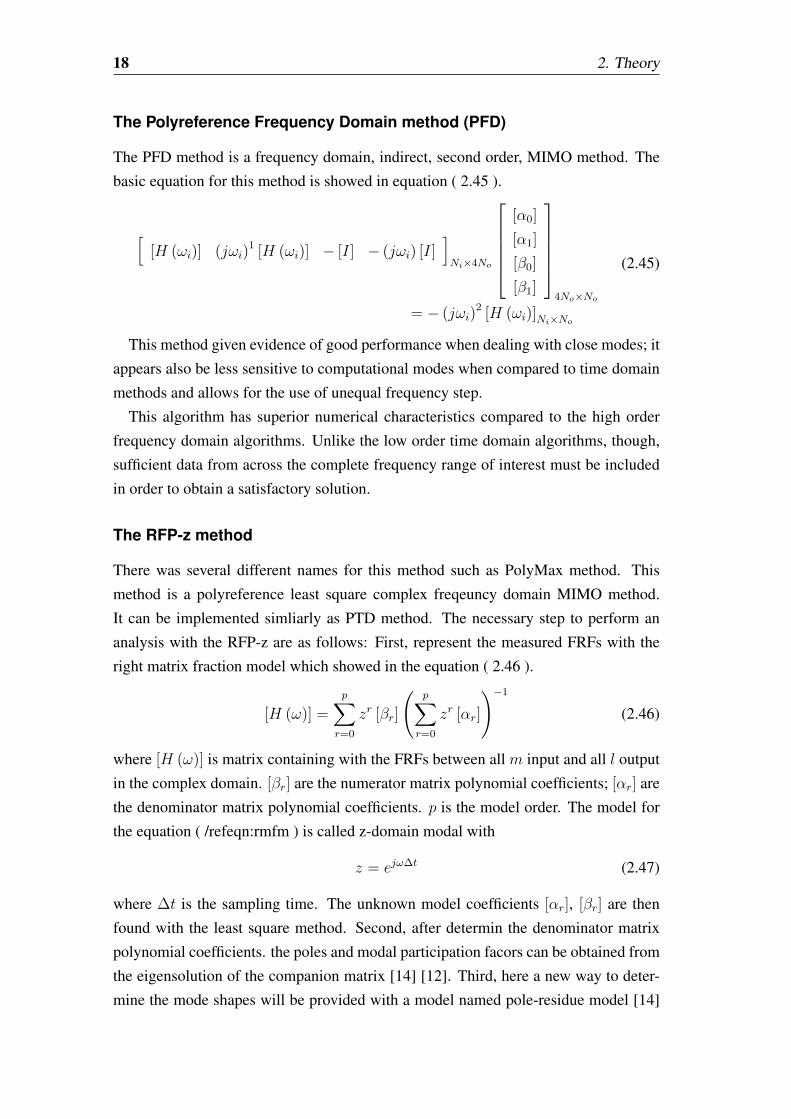
The Polyreference Frequency Domain method (PFD)
The PFD method is a frequency domain, indirect, second order, MIMO method. The
basic equation for this method is showed in equation ( 2.45 ).
[[H (ωi)] (jωi)
1 [H (ωi)] − [I] − (jωi) [I]]Ni×4No
[α0]
[α1]
[β0]
[β1]
4No×No
= − (jωi)2 [H (ωi)]Ni×No
(2.45)
This method given evidence of good performance when dealing with close modes; it
appears also be less sensitive to computational modes when compared to time domain
methods and allows for the use of unequal frequency step.
This algorithm has superior numerical characteristics compared to the high order
frequency domain algorithms. Unlike the low order time domain algorithms, though,
sufficient data from across the complete frequency range of interest must be included
in order to obtain a satisfactory solution.
The RFP-z method
There was several different names for this method such as PolyMax method. This
method is a polyreference least square complex freqeuncy domain MIMO method.
It can be implemented simliarly as PTD method. The necessary step to perform an
analysis with the RFP-z are as follows: First, represent the measured FRFs with the
right matrix fraction model which showed in the equation ( 2.46 ).
[H (ω)] =
p∑r=0
zr [βr]
(p∑r=0
zr [αr]
)−1
(2.46)
where [H (ω)] is matrix containing with the FRFs between all m input and all l output
in the complex domain. [βr] are the numerator matrix polynomial coefficients; [αr] are
the denominator matrix polynomial coefficients. p is the model order. The model for
the equation ( /refeqn:rmfm ) is called z-domain modal with
z = ejω∆t (2.47)
where ∆t is the sampling time. The unknown model coefficients [αr], [βr] are then
found with the least square method. Second, after determin the denominator matrix
polynomial coefficients. the poles and modal participation facors can be obtained from
the eigensolution of the companion matrix [14] [12]. Third, here a new way to deter-
mine the mode shapes will be provided with a model named pole-residue model [14]
2.3. FE Simulation 19
[12]. the mode shapes can be obtained by solving the pole-residue model with the
linear least square method.
The advantage is that, the method will yields very clear consistancy diagram than
other method, in other words, it is easy to the physical poles from the diagram. This is
because the non-physical poles will be estimated with negative damping ratio so that
the diagram only contains the physical poles. And this method can deal with large
frequency range and large model order, since it does not suffer from the numerical
problems as it is in the z-domain. The method shows very good performance for the
systems with high damping ratios [12].
2.2.3. Universal File Format (UFF)
The experimental data collected from the experiment is stored in UFF files. The detail
format can be found on the website of UC-SDRC and reference [25].
Universal File Formats (UFF) were originally developed by the Structural Dynamics
Research Corporation (SDRC) in the late 1960s and early 1970s to facilitate data trans-
fer between Computer Aided Design (CAD) and Computer Aided Test (CAT) in order
to make the Computer Aided Engineering (CAE) easier. SDRC continues to support
and use the UFF as part of their CAE software.
The formats were originally developed as 80 character in each line, ASCII records
that occur in a specific order according to each UFF. As computer files became rou-
tinely available, single UFF were concatenated into computer file structures. Recently,
a hybrid UF file structure (UF Dataset 58 Binary) was developed. The data stored in
this format is twice as small as the former format.
The use of the Universal File Format as a "standard" has been of great value to the
experimental dynamics (vibration and acoustic) community, particularly in the area of
modal analysis.
2.3. FE Simulation
The details of this part can be found on the reference [23], reference [9], reference [11]
and reference [4].
The joint connections can be divided into normally loaded and tangentially loaded
joints. Generally, the damping in normally loaded joints is very small compared to
tangentially loaded since the relative displacement of the two parts of the joint is the
main factor wich influence the damping and there will be relatively small displacement
in the normal direction [9].
20 2. Theory
It has been shown by experimental investigations that joint damping is nearly fre-
quency independent. Similar results have been shown for material damping in metals,
where the main cause of dissipation is inner friction in the material [23]. During the FE
modeling the constant hysteresis damping will be used. The method uses frequency-
independent damping and linear joint stiffness parameters in order to predict the vi-
bration response of structures. This allows fast prediction of the eigenfrequencies and
modal damping factors of structures before there exists a physical prototype for exper-
imental testing [9].
The thin-layer element is a method making use of thin layer elements for interfaces
and joints. The basic idea is that the behavior near the interface involves a finite thin
zone. The response of that zone is different from the behavior of the surrounding
materials and it is achieved by considering appropriate constitutive law for the element
[7].
During the calculation of the vibrational characteristics of the structure with the
FEM, the following equation of motion for an undamped system is used.
[M ] u+ [K] u = 0 (2.48)
Where [M ] is a mass matrix, [K] is a real valued stiffness matrix, and u is the
displacement vector. Eigenvalues and eigenmodes can be determined by performing
a numerical modal analysis with ANSYS. For the case of utilizing constant hysteresis
damping, it will be add to the stiffness matrix as a complex-valued product of dissipa-
tion multiplayer αi and βi for the material and the joint damping.
[K∗] = [K] + j [C] = [K] + jn∑i=1
αi[Kmateriali
]+ j
n∑i=1
βi
[Kjointj
](2.49)
where for the considered system with low damping αi, βi 1 , this problem can
be solved by harmonic analysis in ANSYS. And in this case modal damping for the
structure can be estimated form the FRF obtained from the harmonic analysis.
Simulating with ANSYS, The damping matrix [C] is used in harmonic analyses. In
its most general form, it is showed in equation ( 2.50 ). The detail of this part can be
found in reference [11] and reference [4]
[C] = α [M ] + (β + βc) [K] +Nm∑j=1
[(βmj +
2
Ωβξj
)[Kj]
]+
Ne∑k=1
[Ck] + [Cξ] (2.50)
where
[C] = structure damping matrix
α = mass matrix multiplier (input on ALPHAD command)
2.3. FE Simulation 21
[M ] = structure mass matrix
β = stiffness matrix multiplier (input on BETAD command)
βc = variable stiffness matrix multiplier
[K] = structure stiffness matrix
Nm = number of materials with DAMP or DMPR input
βmj = stiffness matrix multiplier for material j (input as DAMP on MP command)
βξj = constant (frequency-independent) stiffness matrix coefficient for material j
(input as DMPR on MP command)
Ω = circular excitation frequency
Kj = portion of structure stiffness matrix based on material j
Ne = number of elements with specified damping
Ck = element damping matrix
Cξ = frequency-dependent damping matrix
For the simulation, α and the βξj is related to complex-value stiffness coefficients αiand βi in equation ( 2.49 ), since βξj is frequency-independent and can reperesent the
damping of the material with constant constant hysteresis.
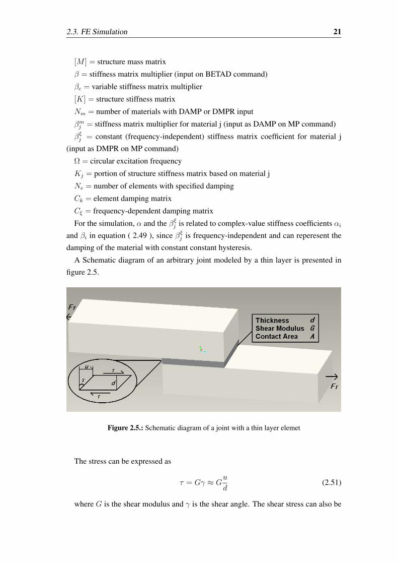
A Schematic diagram of an arbitrary joint modeled by a thin layer is presented in
figure 2.5.
Figure 2.5.: Schematic diagram of a joint with a thin layer elemet
The stress can be expressed as
τ = Gγ ≈ Gu
d(2.51)
where G is the shear modulus and γ is the shear angle. The shear stress can also be
22 2. Theory
estimated by the ratio of tangential force F and area of the contact A.
τ =F
A(2.52)
Combining Equations ( 2.51 ) and ( 2.52 ), the force can be calculated
F ≈ GA
du = ku (2.53)
It is important to recognize that the characteristics of the joint‘s interface that is
represented by the thin layer elements is orthotropic. There are significant differences
in tangential and normal behavior of the joint
From equation ( 2.53 ) the shear modulus can be approximated as
G =kd
A(2.54)
The damping coefficient ξ for the joint and stiffness k can be obtained from the
joint patch experiment.The material damping can also be determined by experimental
approach with half-width value method. The related experiments are introduced in
reference [23]
For the simulation, the orthotropic material has been chosen and the constitutive
material law can be expressed in the equation ( 2.55 ).
σxx
σyy
σzz
σxy
σyz
σzx
=
E11 E12 E13 0 0 0
E22 E23 0 0 0
E33 0 0 0
E44 0 0
E55 0
E66
εxx
εyy
εzz
εxy
εyz
εzx
(2.55)
The off-diagonal terms (E12, E13, E23) are zero for physical reasons (there is no
transversal constriction invoked by the contact interface). Also, since the interface
has no stiffness in and directions (parallel to the joint‘s surface), the terms E11 and
E22 disappear. E33 represents the normal stiffness, whereas E55 = E66 = G define
the tangential stiffness of the joint. Since the joint exhibits no stiffness for in-plane
shearing, E44 is also zero. For numerical reasons all diagonal terms in equation ( 2.55
) must be different from zero. Thus, in the calculation the values of E11, E22 and E44
are set to some small values.
And in this thesis, the interrelations between the joint characteristics and the material
parameters such as shear module G and βξj will be figured out.

3. Design the System
For this thesis, design a mechanical system which can perform different joint properties
is compulsory, in order to investigate the relationship between joint properties and the
structural dynamic properties. In this chapter design and verification of a mechanical
structure will be carried out with the help of ANSYS.
3.1. Criteria
There are several criteria need to be satisfied.
• The maximum mass of the total system is 20kg. The mass must be big enough
to avoid the massloading effect of the accelerometers or the bolts. however, it
cannot be exceed the capability of experimenter as the structure must hanged
during the experiment.
• The 1st eigenfrequency must between 100Hz and 400Hz. The eigenfrequencies
of the strucutre surpposed to be lies in the low frequency range.
• Different pressure distribution must be counted in. and this can be relized with
different bolt spacing. In this thesis, the pressure distribution is one of the im-
portant factors need to be investigated which influence the dynamic properties
of the structure.
• The structure must assembled in several different ways. This related to the capa-
bility of the structure to perform many different joint characteristics.
• The structure must as simple as possible. So that the problem will be simply
described and the relations between the joint characteristics and dynamic prop-
erties of the structure can be clearly expressed.
24 3. Design the System
3.2. Design
3.2.1. Assumption
Here, arbitrary structures and dimensions are given and checked with ANSYS, the
structures need to satisfy the criteria discussed in section 3.1. The assumptions for
the simulation with ANSYS must be made before design. Firts, the whole structure
assumed to be welded together. Second, all parts has the same material properties as the
eigenfrequecy and modes shape did not depend too much on the damping properties.
Under this two assumption the simulation will be carried out to verify whether the
designed structure satisfies the criteria or not. The ANSYS command can be checked
in reference [4]. and the command stream which used to set up the structure is showed
in Appendix A.2.
3.2.2. Sturcture
After several times of simulation and redesign process, finally, the structure of system
determined to be constructed with two separate parts, named structure B and structure
C. The detail size, shape can be found in the Appendix A.3. The design of the shape of
the structure, the joint and the ways of assembly can be referenced from the reference
[8].
In this thesis, the Structure B and Structure C was used to form a structure with bolt
which showed in figure 3.1.
With the structure designed, several different assemblies can be constructed and can
also perform joints with different characteristics.
3.2.3. Simulation
The necessary steps for the simulation is: first, decide the mesh size for the following
step; second, perform the modal analysis to check whether the structure satisfy the
criteria or not. Mesh size affects the accuracy of the simulation. As the mesh size
getting smaller, the finite elements model will tends to real model and the simulation
results will approach the exact values.
Determine the Mesh Density
As the main structure which will create the major parts of the elements is Structure B,
the influence that caused by the mesh size of this structure must be investigated. And
here the structure A (figure 3.2 and Appendix A.3) designed and used to verify the
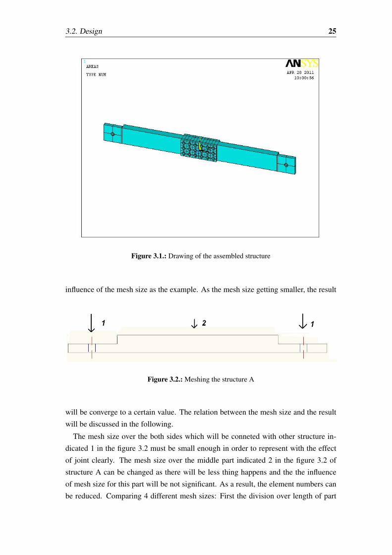
3.2. Design 25
Figure 3.1.: Drawing of the assembled structure
influence of the mesh size as the example. As the mesh size getting smaller, the result
Figure 3.2.: Meshing the structure A
will be converge to a certain value. The relation between the mesh size and the result
will be discussed in the following.
The mesh size over the both sides which will be conneted with other structure in-
dicated 1 in the figure 3.2 must be small enough in order to represent with the effect
of joint clearly. The mesh size over the middle part indicated 2 in the figure 3.2 of
structure A can be changed as there will be less thing happens and the the influence
of mesh size for this part will be not significant. As a result, the element numbers can
be reduced. Comparing 4 different mesh sizes: First the division over length of part
26 3. Design the System
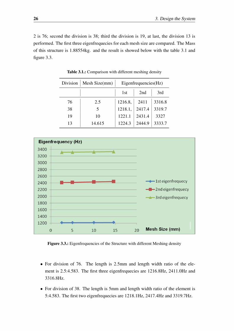
2 is 76; second the division is 38; third the division is 19, at last, the division 13 is
performed. The first three eigenfrequecies for each mesh size are compared. The Mass
of this structure is 1.88554kg. and the result is showed below with the table 3.1 and
figure 3.3.
Table 3.1.: Comparison with different meshing density
Division Mesh Size(mm) Eigenfrequencies(Hz)
1st 2nd 3rd
76 2.5 1216.8, 2411 3316.8
38 5 1218.1, 2417.4 3319.7
19 10 1221.1 2431.4 3327
13 14.615 1224.3 2444.9 3333.7
Figure 3.3.: Eigenfrequencies of the Structure with different Meshing density
• For division of 76. The length is 2.5mm and length width ratio of the ele-
ment is 2.5:4.583. The first three eigenfrequecies are 1216.8Hz, 2411.0Hz and
3316.8Hz.
• For division of 38. The length is 5mm and length width ratio of the element is
5:4.583. The first two eigenfrequecies are 1218.1Hz, 2417.4Hz and 3319.7Hz.
3.2. Design 27
• C. For division of 19. The length is 10mm and length width ratio of the ele-
ment is 10:4.583. The first two eigenfrequecies are 1221.1Hz, 2431.4Hz and
3327.0Hz.
• For division of 13. The length is 14.615mm and length width ratio of the el-
ement is 14.615:4.583. The first two eigenfrequecies are 1224.3Hz, 2444.9Hz
and 3333.7Hz.
The result can be found in the figure 3.3 that the mesh will not influence the result
too much, and the division of 25 will be chosen in order to make sure not only the
accuracy of the result, but also reduce the calculating time.
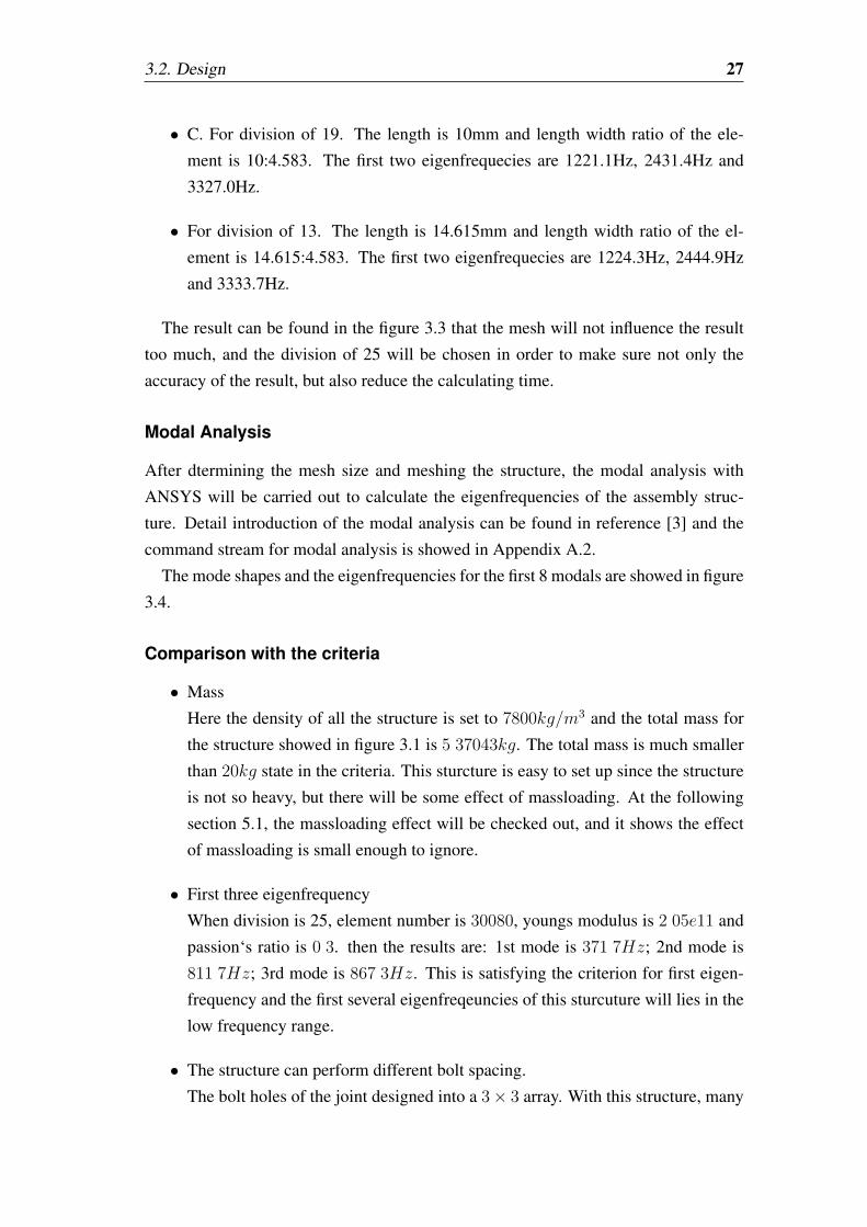
Modal Analysis
After dtermining the mesh size and meshing the structure, the modal analysis with
ANSYS will be carried out to calculate the eigenfrequencies of the assembly struc-
ture. Detail introduction of the modal analysis can be found in reference [3] and the
command stream for modal analysis is showed in Appendix A.2.
The mode shapes and the eigenfrequencies for the first 8 modals are showed in figure
3.4.
Comparison with the criteria
• Mass
Here the density of all the structure is set to 7800kg/m3 and the total mass for
the structure showed in figure 3.1 is 5 37043kg. The total mass is much smaller
than 20kg state in the criteria. This sturcture is easy to set up since the structure
is not so heavy, but there will be some effect of massloading. At the following
section 5.1, the massloading effect will be checked out, and it shows the effect
of massloading is small enough to ignore.
• First three eigenfrequency
When division is 25, element number is 30080, youngs modulus is 2 05e11 and
passion‘s ratio is 0 3. then the results are: 1st mode is 371 7Hz; 2nd mode is
811 7Hz; 3rd mode is 867 3Hz. This is satisfying the criterion for first eigen-
frequency and the first several eigenfreqeuncies of this sturcuture will lies in the
low frequency range.
• The structure can perform different bolt spacing.
The bolt holes of the joint designed into a 3× 3 array. With this structure, many
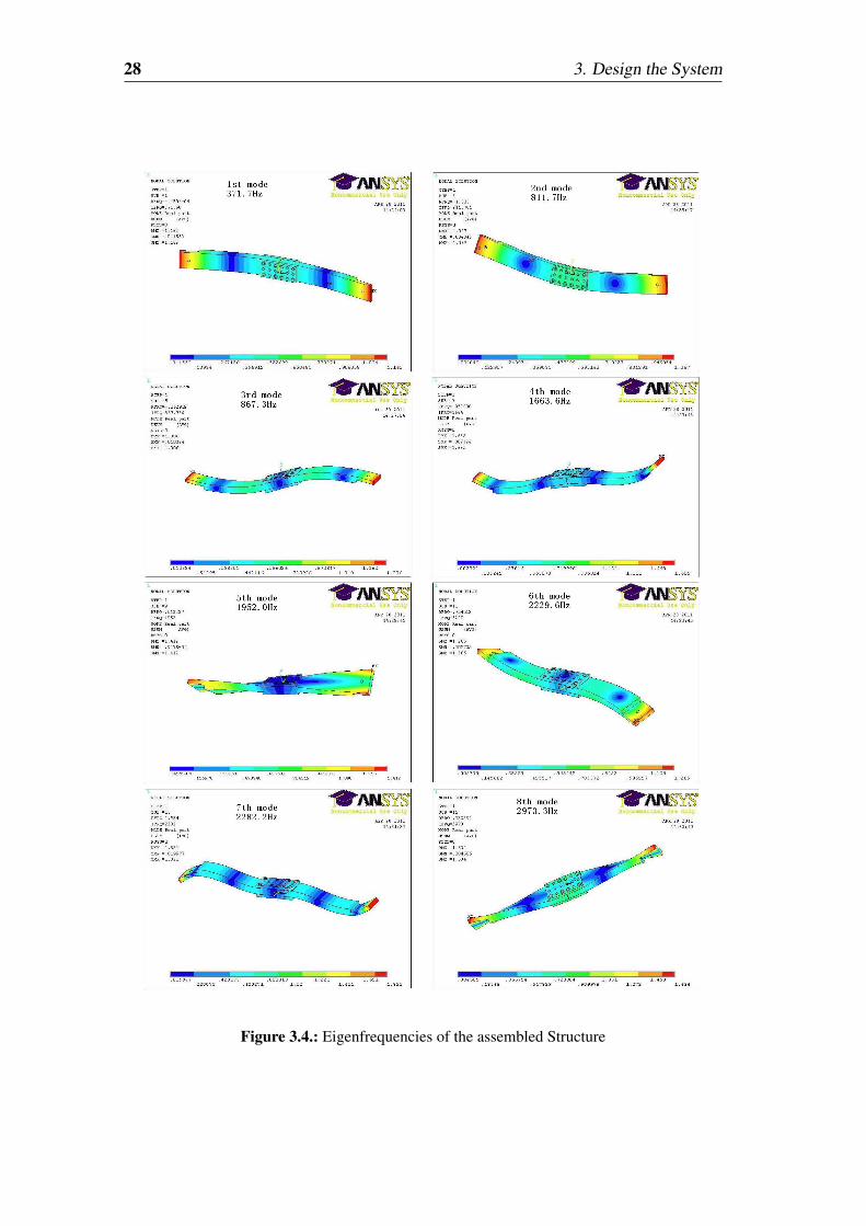
28 3. Design the System
Figure 3.4.: Eigenfrequencies of the assembled Structure

3.2. Design 29
different bolt position for the joint can be applied, which will be discussed in
section 5.1.3. This means the structure will provide different types of pressure
distributions.
• The structure can perform several different assembly.
The strucutres can be assembled in many different ways, with the different joint
types. For the thesis, only the structure showed in figure 3.1 will be used.
• The structure is very simple.
The structure can be nearly considered as several bars conneting to each other
with the joints. Each structure can be considered as linear system, and the struc-
tures will be satisfys the assumptions for the analytical and experimental modal
analysis state in chapter 2.
The structures designed are satisfying the criteria and can be used in the investigation
with experimental modal analysis.

4. Analytical approach
For the thesis, the X-Modal II which is developed by the Structural Dynamics Research
Laboratory of University of Cincinnati (UC-SDRL) will be utilized. This software
provides 6 kinds of modal parameter estimation methods. Which method is the more
suitable one for the analytical data sets with the low damping will be discussed with
the analytical approach in this chapter. The analytical data sets with known properties
are generated using the MATLAB code (see appendix A.1). And the analytical data
sets will be transferred into Universal File Format (UFF) in order to be loaded into
X-Modal II. After calculating the poles and vectors, the poles must be chosen from
many possible solutions ( section 4.2.1 ). Two techniques used to select the poles will
be cpmpared. The different modal parameter estimation methods will be investigated
with respect to several different aspects such as the pole selecting method and the
frequency resolution to determine the more suitable method for the data sets with low
damping properties.
4.1. Analytical Data Sets Creation
First, the Single Input Single Output (SISO) modal model is constructed to generate
analytical data sets with different frequency resolutions and these data sets will be used
to compare the two methods used to select poles and vectors in X-Modal II. Investi-
gation of the influences caused by different frequency resolutions also requires these
data sets. For the frequency domain method, the Multi Input Multi Output (MIMO)
modal model used to generate analytical data sets are utilized to determine the better
pole selecting method and the frequency resolution for the following investigations.
Second, the MIMO Spatial model with the chosen frequency resolution will be pro-
vided. For the modal parameter estimation, the pole selecting method chosen by the
first step will be applied. These analytical data sets obtained from the MIMO spatial
model will be used to investigate the different modal parameter estimation methods.
At the end, the MIMO modal model with noise is used to generated the analytical
data sets to investigate the influence caused by the noise with different amplitude as
well as determine which modal parameter estimation method can overcome the uncer-
32 4. Analytical approach
tainty of the experimental and analytical data sets.
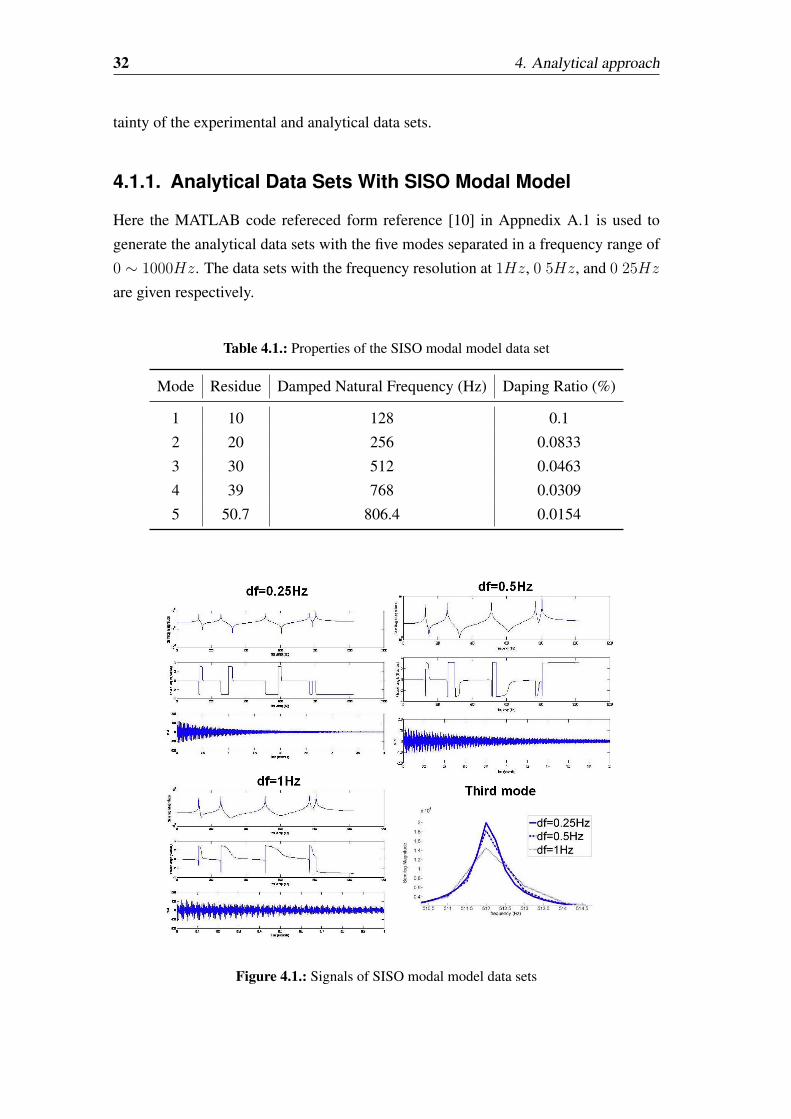
4.1.1. Analytical Data Sets With SISO Modal Model
Here the MATLAB code refereced form reference [10] in Appnedix A.1 is used to
generate the analytical data sets with the five modes separated in a frequency range of
0 ∼ 1000Hz. The data sets with the frequency resolution at 1Hz, 0 5Hz, and 0 25Hz
are given respectively.
Table 4.1.: Properties of the SISO modal model data set
Mode Residue Damped Natural Frequency (Hz) Daping Ratio (%)
1 10 128 0.1
2 20 256 0.0833
3 30 512 0.0463
4 39 768 0.0309
5 50.7 806.4 0.0154
Figure 4.1.: Signals of SISO modal model data sets

4.1. Analytical Data Sets Creation 33
The plots of Impulse Response Function (IRF), Frequency Response Function (FRF)
and Phase angle of analytical data sets with the modal properties showed in table 4.1 at
different frequency resolutions are presented in the figure 4.1. At the last of the figure
4.1, the third mode of the FRFs with different freqeucny resolution have been overlaid.
From this, the results that the frequency resolution do not change the eigenfreqeucny
too much, but the damping will be greatly affected for the method use the frequency
domain data sets can be derived out.
The data sets created will be transferred into universal file format using the MAT-
LAB code [6]. These data sets are used to determine the suitable frequency resolution
for the following analytical models.
4.1.2. Analytical Data Sets With MIMO Modal Model
Here the MIMO modal model will be created with the modal frequencies and mode
shapes. The transformation matrix introduced in equantion ( 2.25 ) which will used
to creat the MIMO system can be constructed with the mode shapes as columns. The
modal damping properties and damped natural frequencies of this model are the same
as the table 4.1. Here the transformation matrix of the original system will be given as
equation ( 4.1 ).
ψ =
−10 −10 −10 −10 −10
5 10 5 5 −5
10 0 −15 0 10
5 −10 5 −5 −5
−10 10 −10 10 −10
(4.1)
The frequency resolution is 1Hz which will be determined in the section 4.2.2. These
data sets are used to find out what kind of influences will be caused by the different
noise amplitudes.
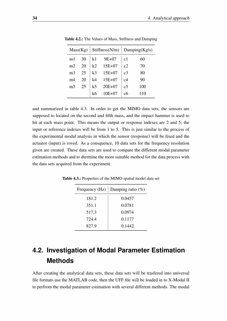
4.1.3. Analytical Data Sets With MIMO Spatial Model
The spatial model is developed form the structure showed in figure 2.2. The degree
of freedom (DOF) for this system is five. The system contains five mass points, four
damping and four stiffness which are between each mass as well as two damping and
two stiffness which are between the first and last mass and the environments. The
mass, damping and stiffness will be provided in table 4.2 for the spatial model.
Here the first five modes lie in the frequency range of 0 to 1000Hz. The analytical
data sets with MIMO spatial model are generated with the above physical parameters
such as mass, stiffness and damping, and the modal properties can be calculated out
34 4. Analytical approach
Table 4.2.: The Values of Mass, Stiffness and Damping
Mass(Kg) Stiffness(N/m) Damping(Kg/s)
m1 30 k1 9E+07 c1 60
m2 20 k2 15E+07 c2 70
m3 25 k3 15E+07 c3 80
m4 20 k4 15E+07 c4 90
m5 25 k5 20E+07 c5 100
k6 10E+07 c6 110
and summarized in table 4.3. In order to get the MIMO data sets, the sensors are
supposed to located on the second and fifth mass, and the impact hammer is used to
hit at each mass point. This means the output or response indexes are 2 and 5; the
input or reference indexes will be from 1 to 5. This is just similar to the process of
the experimental modal analysis in which the sensor (response) will be fixed and the
actuator (input) is roved. As a consquence, 10 data sets for the frequency resolution
given are created. These data sets are used to compare the different modal parameter
estimation methods and to dtermine the more suitable method for the data process with
the data sets acquired from the experiment.
Table 4.3.: Properties of the MIMO spatial model data set
Frequency (Hz) Damping ratio (%)
181.2 0.0457
351.1 0.0781
517.3 0.0974
724.4 0.1177
827.9 0.1442
4.2. Investigation of Modal Parameter Estimation
Methods
After creating the analytical data sets, these data sets will be trasfered into universal
file formats use the MATLAB code, then the UFF file will be loaded in to X-Modal II
to perfrom the modal parameter estimation with several different methods. The modal
4.2. Investigation of Modal Parameter Estimation Methods 35
parameters can be obtained in terms of eigenfrequencies (damped natural frequencies)
and modal damping ratio. The exact eigenfrequecies and the damping ratio are already
known in the section 4.1, and the methods will be investigated by the comparison of
the exact value and the values acquired from the X-Modal II. This detail procedure can
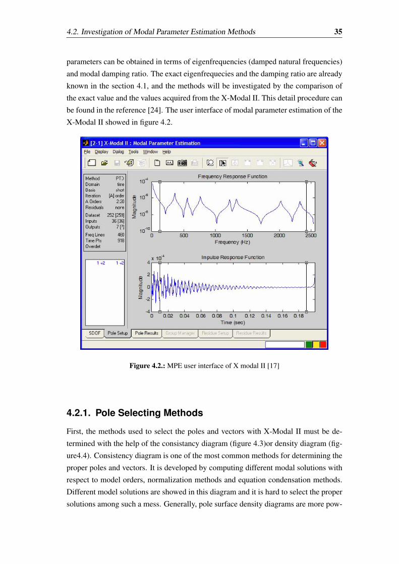
be found in the reference [24]. The user interface of modal parameter estimation of the
X-Modal II showed in figure 4.2.
Figure 4.2.: MPE user interface of X modal II [17]
4.2.1. Pole Selecting Methods
First, the methods used to select the poles and vectors with X-Modal II must be de-
termined with the help of the consistancy diagram (figure 4.3)or density diagram (fig-
ure4.4). Consistency diagram is one of the most common methods for determining the
proper poles and vectors. It is developed by computing different modal solutions with
respect to model orders, normalization methods and equation condensation methods.
Different model solutions are showed in this diagram and it is hard to select the proper
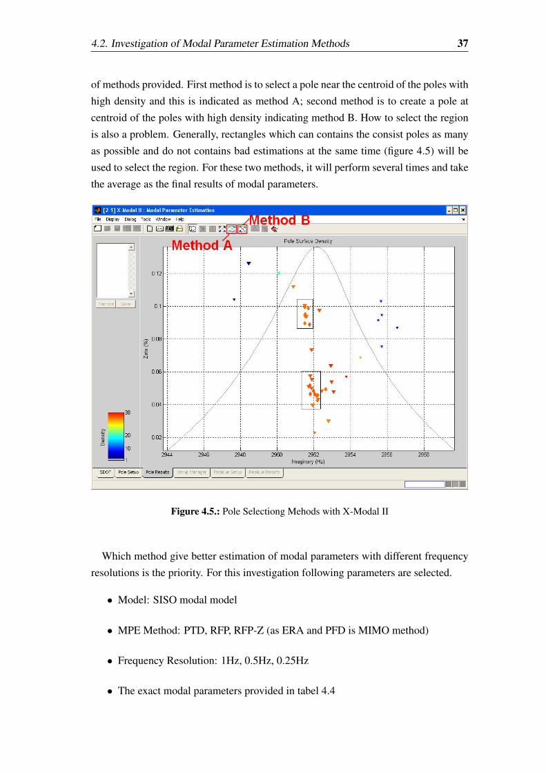
solutions among such a mess. Generally, pole surface density diagrams are more pow-
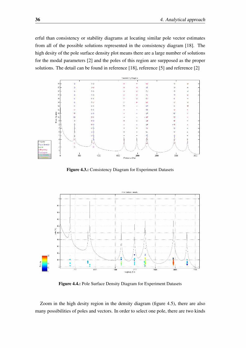
36 4. Analytical approach
erful than consistency or stability diagrams at locating similar pole vector estimates
from all of the possible solutions represented in the consistency diagram [18]. The
high desity of the pole surface density plot means there are a large number of solutions
for the modal parameters [2] and the poles of this region are surpposed as the proper
solutions. The detail can be found in reference [18], reference [5] and reference [2]
Figure 4.3.: Consistency Diagram for Experiment Datasets
Figure 4.4.: Pole Surface Density Diagram for Experiment Datasets
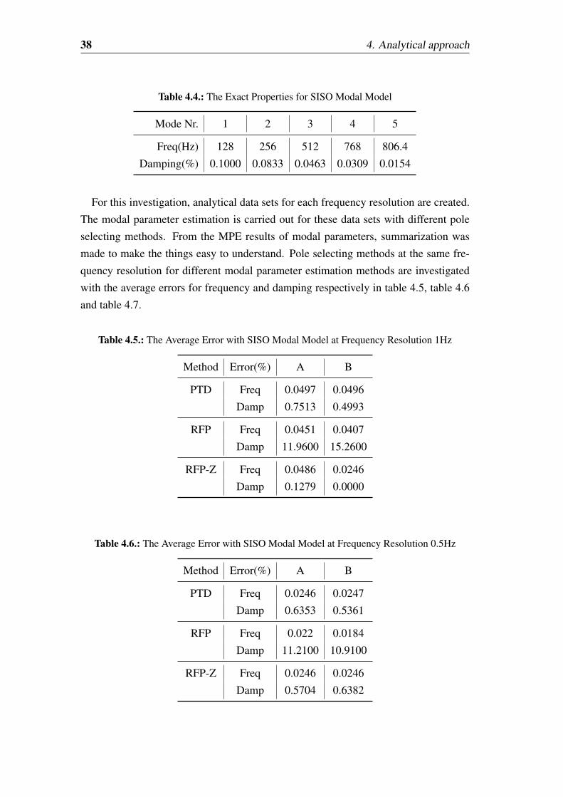
Zoom in the high desity region in the density diagram (figure 4.5), there are also
many possibilities of poles and vectors. In order to select one pole, there are two kinds
4.2. Investigation of Modal Parameter Estimation Methods 37
of methods provided. First method is to select a pole near the centroid of the poles with
high density and this is indicated as method A; second method is to create a pole at
centroid of the poles with high density indicating method B. How to select the region
is also a problem. Generally, rectangles which can contains the consist poles as many
as possible and do not contains bad estimations at the same time (figure 4.5) will be
used to select the region. For these two methods, it will perform several times and take
the average as the final results of modal parameters.
Figure 4.5.: Pole Selectiong Mehods with X-Modal II
Which method give better estimation of modal parameters with different frequency
resolutions is the priority. For this investigation following parameters are selected.
• Model: SISO modal model
• MPE Method: PTD, RFP, RFP-Z (as ERA and PFD is MIMO method)
• Frequency Resolution: 1Hz, 0.5Hz, 0.25Hz
• The exact modal parameters provided in tabel 4.4
38 4. Analytical approach
Table 4.4.: The Exact Properties for SISO Modal Model
Mode Nr. 1 2 3 4 5
Freq(Hz) 128 256 512 768 806.4
Damping(%) 0.1000 0.0833 0.0463 0.0309 0.0154
For this investigation, analytical data sets for each frequency resolution are created.
The modal parameter estimation is carried out for these data sets with different pole
selecting methods. From the MPE results of modal parameters, summarization was
made to make the things easy to understand. Pole selecting methods at the same fre-
quency resolution for different modal parameter estimation methods are investigated
with the average errors for frequency and damping respectively in table 4.5, table 4.6
and table 4.7.
Table 4.5.: The Average Error with SISO Modal Model at Frequency Resolution 1Hz
Method Error(%) A B
PTD Freq 0.0497 0.0496
Damp 0.7513 0.4993
RFP Freq 0.0451 0.0407
Damp 11.9600 15.2600
RFP-Z Freq 0.0486 0.0246
Damp 0.1279 0.0000
Table 4.6.: The Average Error with SISO Modal Model at Frequency Resolution 0.5Hz
Method Error(%) A B
PTD Freq 0.0246 0.0247
Damp 0.6353 0.5361
RFP Freq 0.022 0.0184
Damp 11.2100 10.9100
RFP-Z Freq 0.0246 0.0246
Damp 0.5704 0.6382
4.2. Investigation of Modal Parameter Estimation Methods 39
Table 4.7.: The Average Error with SISO Modal Model at Frequency Resolution 0.25Hz
Method Error(%) A B
PTD Freq 0.0112 0.0115
Damp 0.7749 0.5588
RFP Freq 0.0109 0.0099
Damp 12.3900 5.9400
RFP-Z Freq 0.012 0.0121
Damp 1.1300 1.1700
From table 4.5, table 4.6 and table 4.7, conclusions can be made that the eigenfre-
qencies will not differ too much with respect to pole selecting methods. For all the
modal parameter estimation methods used and for all the frequency resolutions given,
the method B, which creates a pole at centroid, gives better estimation of the damping
ratio. The method B will provide better estimation since it avarages the poles inside
the rectangle and has the informations about the system. While the method A will only
select one pole near the center of region of square and the results only related to the
rectangle used to select the poles. This will have less information of the system.
4.2.2. Frequency Resolution
From the results above, the effect caused by the frequency resolution with respect to
PTD, RFP and RFP-Z methods can be noticed. The results are written in another way
so that it is easy to understand. For the investigation, the following results will be used.
• Pole selecting method B
Table 4.8.: The Average Error with SISO Modal for Different Frequency Resolutions
Average error (%)
Method PTD RFP RFP-Z
Df Freq Damp Freq Damp Freq Damp
1Hz 0.0496 0.4993 0.0407 15.2600 0.0246 0.0000
0.5Hz 0.0247 0.5361 0.0184 10.9100 0.0246 0.6382
0.25Hz 0.0115 0.5588 0.0099 5.9400 0.0121 1.1700
40 4. Analytical approach
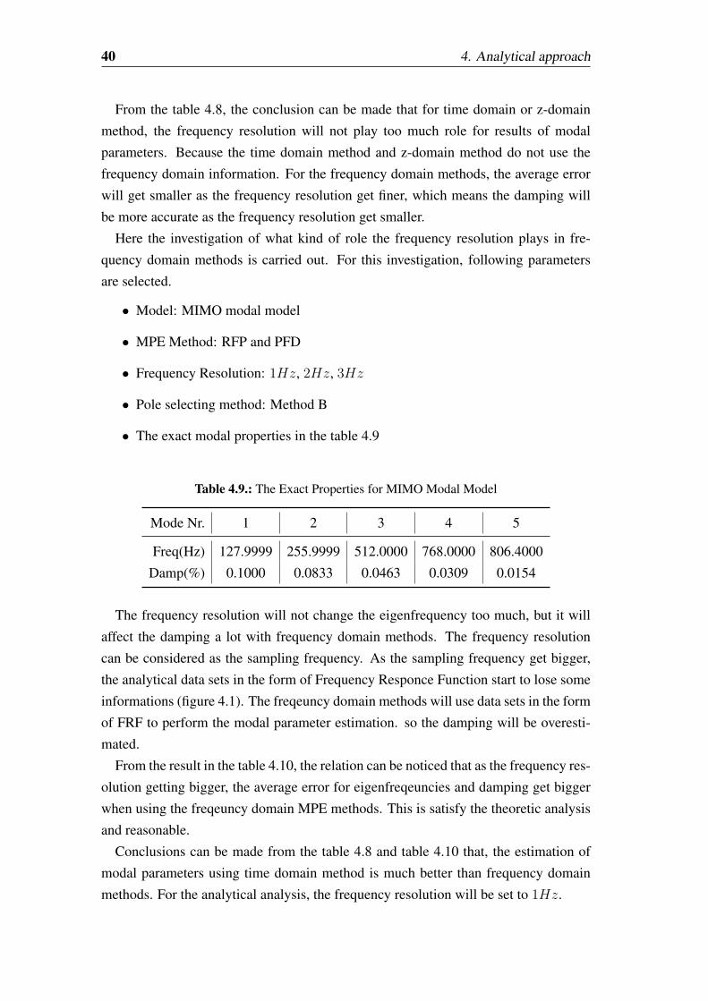
From the table 4.8, the conclusion can be made that for time domain or z-domain
method, the frequency resolution will not play too much role for results of modal
parameters. Because the time domain method and z-domain method do not use the
frequency domain information. For the frequency domain methods, the average error
will get smaller as the frequency resolution get finer, which means the damping will
be more accurate as the frequency resolution get smaller.
Here the investigation of what kind of role the frequency resolution plays in fre-
quency domain methods is carried out. For this investigation, following parameters
are selected.
• Model: MIMO modal model
• MPE Method: RFP and PFD
• Frequency Resolution: 1Hz, 2Hz, 3Hz
• Pole selecting method: Method B
• The exact modal properties in the table 4.9
Table 4.9.: The Exact Properties for MIMO Modal Model
Mode Nr. 1 2 3 4 5
Freq(Hz) 127.9999 255.9999 512.0000 768.0000 806.4000
Damp(%) 0.1000 0.0833 0.0463 0.0309 0.0154
The frequency resolution will not change the eigenfrequency too much, but it will
affect the damping a lot with frequency domain methods. The frequency resolution
can be considered as the sampling frequency. As the sampling frequency get bigger,
the analytical data sets in the form of Frequency Responce Function start to lose some
informations (figure 4.1). The freqeuncy domain methods will use data sets in the form
of FRF to perform the modal parameter estimation. so the damping will be overesti-
mated.
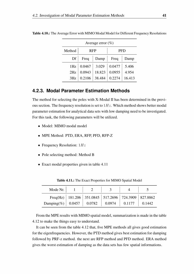
From the result in the table 4.10, the relation can be noticed that as the frequency res-
olution getting bigger, the average error for eigenfreqeuncies and damping get bigger
when using the freqeuncy domain MPE methods. This is satisfy the theoretic analysis
and reasonable.
Conclusions can be made from the table 4.8 and table 4.10 that, the estimation of
modal parameters using time domain method is much better than frequency domain
methods. For the analytical analysis, the frequency resolution will be set to 1Hz.
4.2. Investigation of Modal Parameter Estimation Methods 41
Table 4.10.: The Average Error with MIMO Modal Model for Different Frequency Resolutions
Average error (%)
Method RFP PFD
Df Freq Damp Freq Damp
1Hz 0.0467 3.029 0.0477 5.406
2Hz 0.0943 18.823 0.0955 4.954
3Hz 0.2106 38.484 0.2274 16.413
4.2.3. Modal Parameter Estimation Methods
The method for selecting the poles with X-Modal II has been determined in the previ-
ous section. The frequency resolution is set to 1Hz. Which method shows better modal
parameter estimation for analytical data sets with low damping need to be investigated.
For this task, the following parameters will be utilized.
• Model: MIMO modal model
• MPE Method: PTD, ERA, RFP, PFD, RFP-Z
• Frequency Resolution: 1Hz
• Pole selecting method: Method B
• Exact modal properties given in table 4.11
Table 4.11.: The Exact Properties for MIMO Spatial Model
Mode Nr. 1 2 3 4 5
Freq(Hz) 181.206 351.0845 517.2696 724.3909 827.8862
Damping(%) 0.0457 0.0782 0.0974 0.1177 0.1442
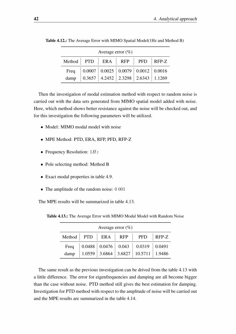
From the MPE results with MIMO spatial model, summarization is made in the table
4.12 to make the things easy to understand.
It can be seen from the table 4.12 that, five MPE methods all gives good estimation
for the eigenfrequencies. However, the PTD method gives best estimation for damping
followed by PRF-z method. the next are RFP method and PFD method. ERA method
gives the worst estimation of damping as the data sets has few spatial informations.
42 4. Analytical approach
Table 4.12.: The Average Error with MIMO Spatial Model(1Hz and Method B)
Average error (%)
Method PTD ERA RFP PFD RFP-Z
Freq 0.0007 0.0025 0.0079 0.0012 0.0016
damp 0.3657 4.2452 2.3298 2.6343 1.1269
Then the investigation of modal estimation method with respect to random noise is
carried out with the data sets generated from MIMO spatial model added with noise.
Here, which method shows better resistance against the noise will be checked out, and
for this investigation the following parameters will be utilized.
• Model: MIMO modal model with noise
• MPE Method: PTD, ERA, RFP, PFD, RFP-Z
• Frequency Resolution: 1Hz
• Pole selecting method: Method B
• Exact modal properties in table 4.9.
• The amplitude of the random noise: 0 001
The MPE results will be summarized in table 4.13.
Table 4.13.: The Average Error with MIMO Modal Model with Random Noise
Average error (%)
Method PTD ERA RFP PFD RFP-Z
Freq 0.0488 0.0476 0.043 0.0319 0.0491
damp 1.0559 3.6864 3.6827 10.5711 1.9486
The same result as the previous investigation can be drived from the table 4.13 with
a little difference. The error for eigenfrequencies and damping are all become bigger
than the case without noise. PTD method still gives the best estimation for damping.
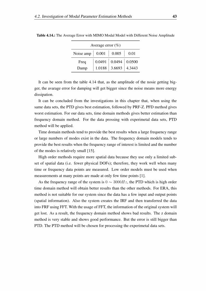
Investigation for PTD method with respect to the amplitude of noise will be carried out
and the MPE results are summarized in the table 4.14.
4.2. Investigation of Modal Parameter Estimation Methods 43
Table 4.14.: The Average Error with MIMO Modal Model with Different Noise Amplitude
Average error (%)
Noise amp 0.001 0.005 0.01
Freq 0.0491 0.0494 0.0500
Damp 1.0188 3.6693 4.3443
It can be seen from the table 4.14 that, as the amplitude of the nosie getting big-
ger, the avarage error for damping will get bigger since the noise means more energy
dissipation.
It can be concluded from the investigations in this chapter that, when using the
same data sets, the PTD gives best estimation, followed by PRF-Z. PFD method gives
worst estimation. For our data sets, time domain methods gives better estimation than
frequency domain method. For the data prossing with experimetal data sets, PTD
method will be applied.
Time domain methods tend to provide the best results when a large frequency range
or large numbers of modes exist in the data. The frequency domain models tends to
provide the best results when the frequency range of interest is limited and the number
of the modes is relatively small [15].
High order methods require more spatial data because they use only a limited sub-
set of spatial data (i.e. fewer physical DOFs); therefore, they work well when many
time or frequency data points are measured. Low order models must be used when
measurements at many points are made at only few time points [1].
As the frequency range of the system is 0 ∼ 3000Hz, the PTD which is high order
time domain method will obtain better results than the other methods. For ERA, this
method is not suitable for our system since the data has a few input and output points
(spatial information). Also the system creates the IRF and then transferred the data
into FRF using FFT. With the usage of FFT, the information of the original system will
get lost. As a result, the frequency domain method shows bad results. The z domain
method is very stable and shows good performance. But the error is still bigger than
PTD. The PTD method will be chosen for processing the experimetal data sets.

5. Experiment and Simulation
After structures designed and manufactured, the experiment is carried out in order
to get the impulse response function or frequency response function used to perform
modal parameter esitmation. First, each part of the total structure separately is tested
in order to adjust the material parameters such as density, Young‘s modulus and Pois-
son‘s ratio. The structures are assembled and suspended with elastic ropes. then free-
free boundary condition experiment are performed by hitting the structure with impact
hammer. The several sets of frequency response function are obtained from the ex-
periment. The data sets are stored in the form of universal file format and loaded into
X-Modal II directly. The PTD method is applied to do the modal parameter estimation
so as to get the dynamic properties. The process is repeated with the assembly with
different joint properties such as different torques and different bolt positions. Then the
commercial software ANSYS is used to doing the structure analysis including modal
analysis and harmonic analysis. The modal analysis is used to verify the relationship
between the joint characteristics such as normal force in the joint and the the pres-
sure distribution of the joint and the modal parameters especially eigenfrequecies; the
harmonic analysis is used to get the frequency response function of the structure, the
data will transfer into universal file format and loaded into X-Modal II to calculate the
modal parameters, here the interrelation between the joint characteristics mentioned
above and damping properties. The thin layer methods will be applied.
5.1. Experiment
The purpose of the experiment is to get the FRF data sets with impact hammer and
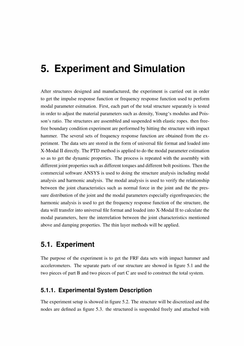
accelerometers. The separate parts of our structure are showed in figure 5.1 and the
two pieces of part B and two pieces of part C are used to construct the total system.
5.1.1. Experimental System Description
The experiment setup is showed in figure 5.2. The structure will be discretized and the
nodes are defined as figure 5.3. the structured is suspended freely and attached with
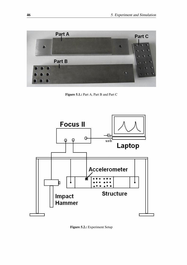
46 5. Experiment and Simulation
Figure 5.1.: Part A, Part B and Part C
Figure 5.2.: Experiment Setup
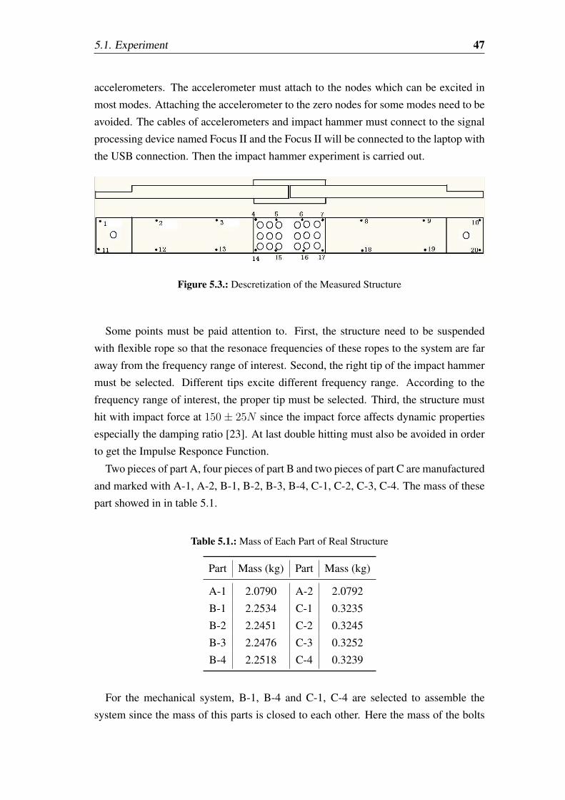
5.1. Experiment 47
accelerometers. The accelerometer must attach to the nodes which can be excited in
most modes. Attaching the accelerometer to the zero nodes for some modes need to be
avoided. The cables of accelerometers and impact hammer must connect to the signal
processing device named Focus II and the Focus II will be connected to the laptop with
the USB connection. Then the impact hammer experiment is carried out.
Figure 5.3.: Descretization of the Measured Structure
Some points must be paid attention to. First, the structure need to be suspended
with flexible rope so that the resonace frequencies of these ropes to the system are far
away from the frequency range of interest. Second, the right tip of the impact hammer
must be selected. Different tips excite different frequency range. According to the
frequency range of interest, the proper tip must be selected. Third, the structure must
hit with impact force at 150 ± 25N since the impact force affects dynamic properties
especially the damping ratio [23]. At last double hitting must also be avoided in order
to get the Impulse Responce Function.
Two pieces of part A, four pieces of part B and two pieces of part C are manufactured
and marked with A-1, A-2, B-1, B-2, B-3, B-4, C-1, C-2, C-3, C-4. The mass of these
part showed in in table 5.1.
Table 5.1.: Mass of Each Part of Real Structure
Part Mass (kg) Part Mass (kg)
A-1 2.0790 A-2 2.0792
B-1 2.2534 C-1 0.3235
B-2 2.2451 C-2 0.3245
B-3 2.2476 C-3 0.3252
B-4 2.2518 C-4 0.3239
For the mechanical system, B-1, B-4 and C-1, C-4 are selected to assemble the
system since the mass of this parts is closed to each other. Here the mass of the bolts
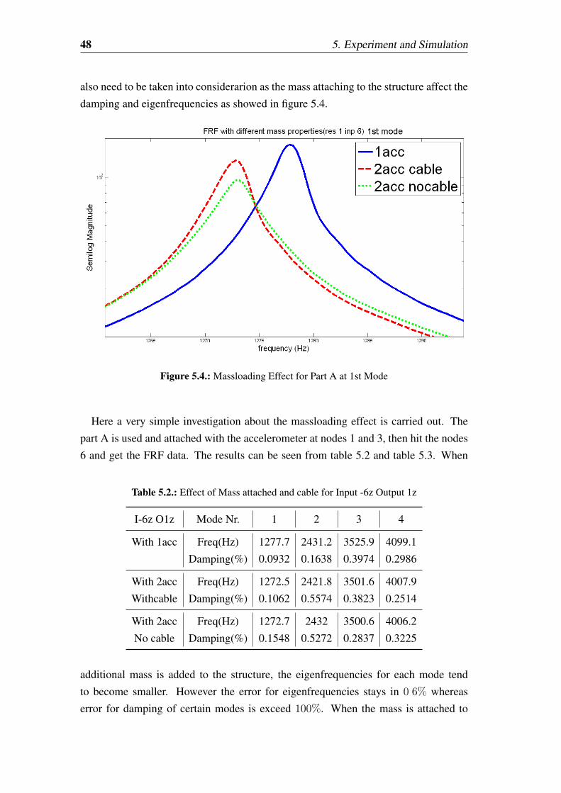
48 5. Experiment and Simulation
also need to be taken into considerarion as the mass attaching to the structure affect the
damping and eigenfrequencies as showed in figure 5.4.
Figure 5.4.: Massloading Effect for Part A at 1st Mode
Here a very simple investigation about the massloading effect is carried out. The
part A is used and attached with the accelerometer at nodes 1 and 3, then hit the nodes
6 and get the FRF data. The results can be seen from table 5.2 and table 5.3. When
Table 5.2.: Effect of Mass attached and cable for Input -6z Output 1z
I-6z O1z Mode Nr. 1 2 3 4
With 1acc Freq(Hz) 1277.7 2431.2 3525.9 4099.1
Damping(%) 0.0932 0.1638 0.3974 0.2986
With 2acc Freq(Hz) 1272.5 2421.8 3501.6 4007.9
Withcable Damping(%) 0.1062 0.5574 0.3823 0.2514
With 2acc Freq(Hz) 1272.7 2432 3500.6 4006.2
No cable Damping(%) 0.1548 0.5272 0.2837 0.3225
additional mass is added to the structure, the eigenfrequencies for each mode tend
to become smaller. However the error for eigenfrequencies stays in 0 6% whereas
error for damping of certain modes is exceed 100%. When the mass is attached to
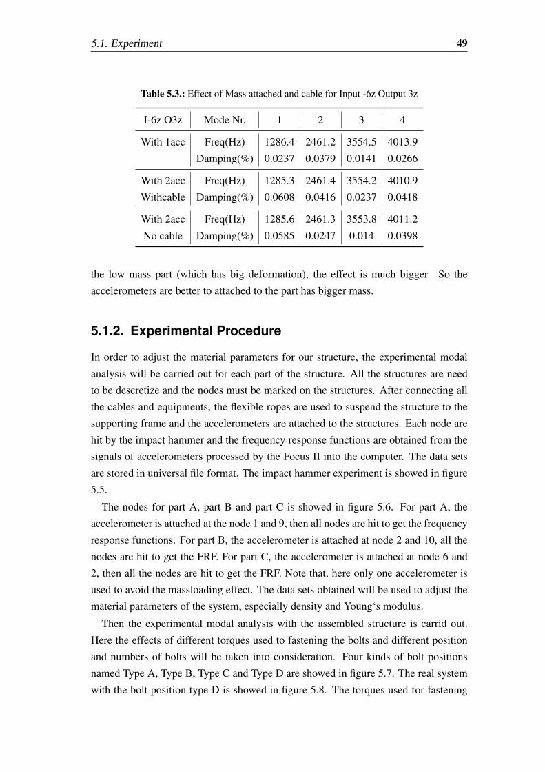
5.1. Experiment 49
Table 5.3.: Effect of Mass attached and cable for Input -6z Output 3z
I-6z O3z Mode Nr. 1 2 3 4
With 1acc Freq(Hz) 1286.4 2461.2 3554.5 4013.9
Damping(%) 0.0237 0.0379 0.0141 0.0266
With 2acc Freq(Hz) 1285.3 2461.4 3554.2 4010.9
Withcable Damping(%) 0.0608 0.0416 0.0237 0.0418
With 2acc Freq(Hz) 1285.6 2461.3 3553.8 4011.2
No cable Damping(%) 0.0585 0.0247 0.014 0.0398
the low mass part (which has big deformation), the effect is much bigger. So the
accelerometers are better to attached to the part has bigger mass.
5.1.2. Experimental Procedure
In order to adjust the material parameters for our structure, the experimental modal
analysis will be carried out for each part of the structure. All the structures are need
to be descretize and the nodes must be marked on the structures. After connecting all
the cables and equipments, the flexible ropes are used to suspend the structure to the
supporting frame and the accelerometers are attached to the structures. Each node are
hit by the impact hammer and the frequency response functions are obtained from the
signals of accelerometers processed by the Focus II into the computer. The data sets
are stored in universal file format. The impact hammer experiment is showed in figure
5.5.
The nodes for part A, part B and part C is showed in figure 5.6. For part A, the
accelerometer is attached at the node 1 and 9, then all nodes are hit to get the frequency
response functions. For part B, the accelerometer is attached at node 2 and 10, all the
nodes are hit to get the FRF. For part C, the accelerometer is attached at node 6 and
2, then all the nodes are hit to get the FRF. Note that, here only one accelerometer is
used to avoid the massloading effect. The data sets obtained will be used to adjust the
material parameters of the system, especially density and Young‘s modulus.
Then the experimental modal analysis with the assembled structure is carrid out.
Here the effects of different torques used to fastening the bolts and different position
and numbers of bolts will be taken into consideration. Four kinds of bolt positions
named Type A, Type B, Type C and Type D are showed in figure 5.7. The real system
with the bolt position type D is showed in figure 5.8. The torques used for fastening
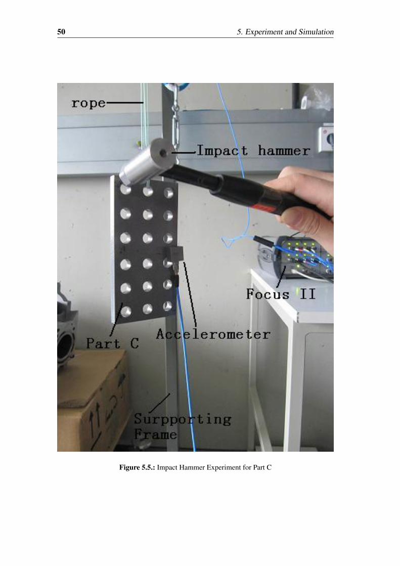
50 5. Experiment and Simulation
Figure 5.5.: Impact Hammer Experiment for Part C
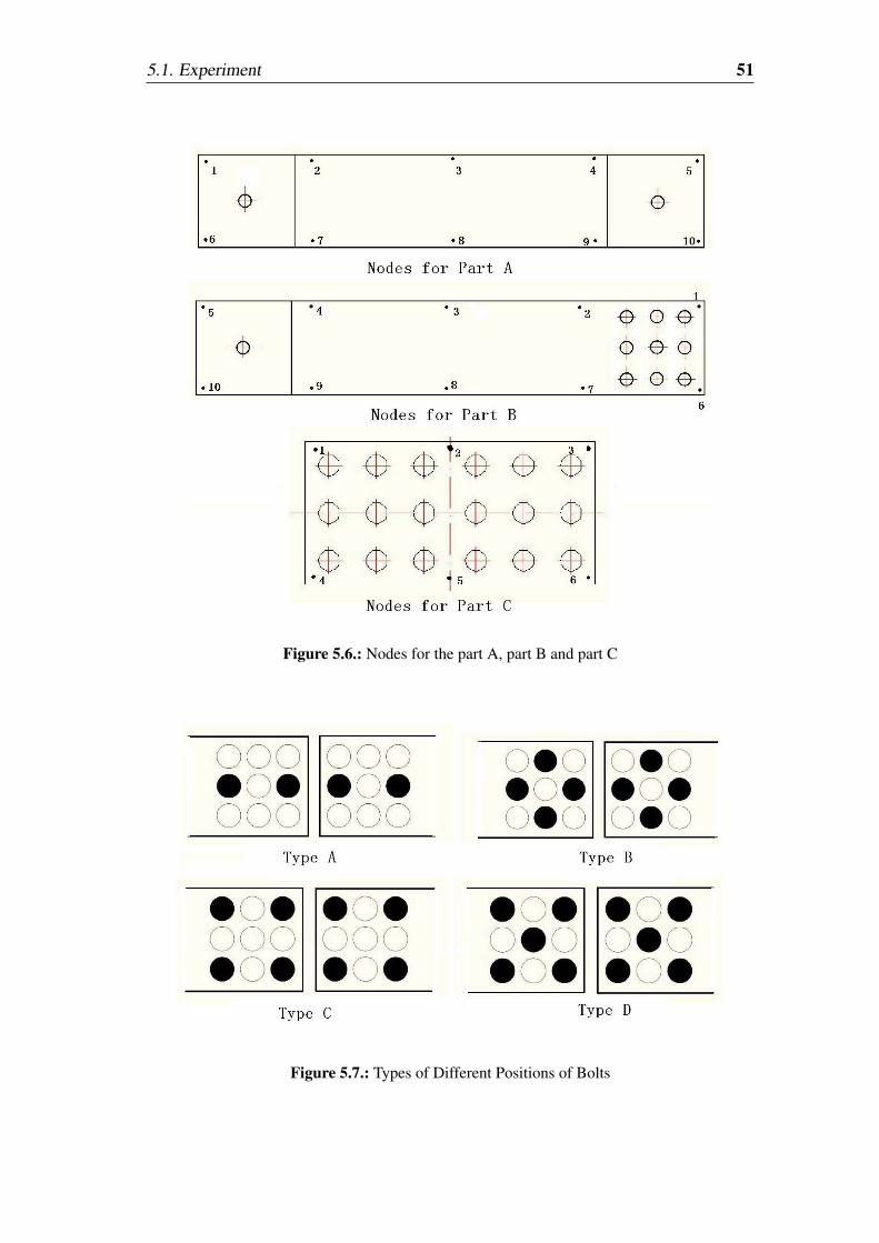
5.1. Experiment 51
Figure 5.6.: Nodes for the part A, part B and part C
Figure 5.7.: Types of Different Positions of Bolts
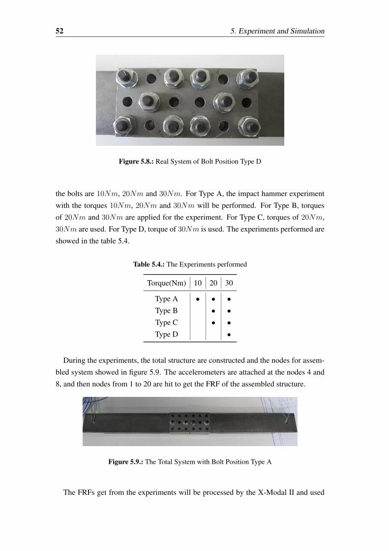
52 5. Experiment and Simulation
Figure 5.8.: Real System of Bolt Position Type D
the bolts are 10Nm, 20Nm and 30Nm. For Type A, the impact hammer experiment
with the torques 10Nm, 20Nm and 30Nm will be performed. For Type B, torques
of 20Nm and 30Nm are applied for the experiment. For Type C, torques of 20Nm,
30Nm are used. For Type D, torque of 30Nm is used. The experiments performed are
showed in the table 5.4.
Table 5.4.: The Experiments performed
Torque(Nm) 10 20 30
Type A • • •Type B • •Type C • •Type D •
During the experiments, the total structure are constructed and the nodes for assem-
bled system showed in figure 5.9. The accelerometers are attached at the nodes 4 and
8, and then nodes from 1 to 20 are hit to get the FRF of the assembled structure.
Figure 5.9.: The Total System with Bolt Position Type A
The FRFs get from the experiments will be processed by the X-Modal II and used
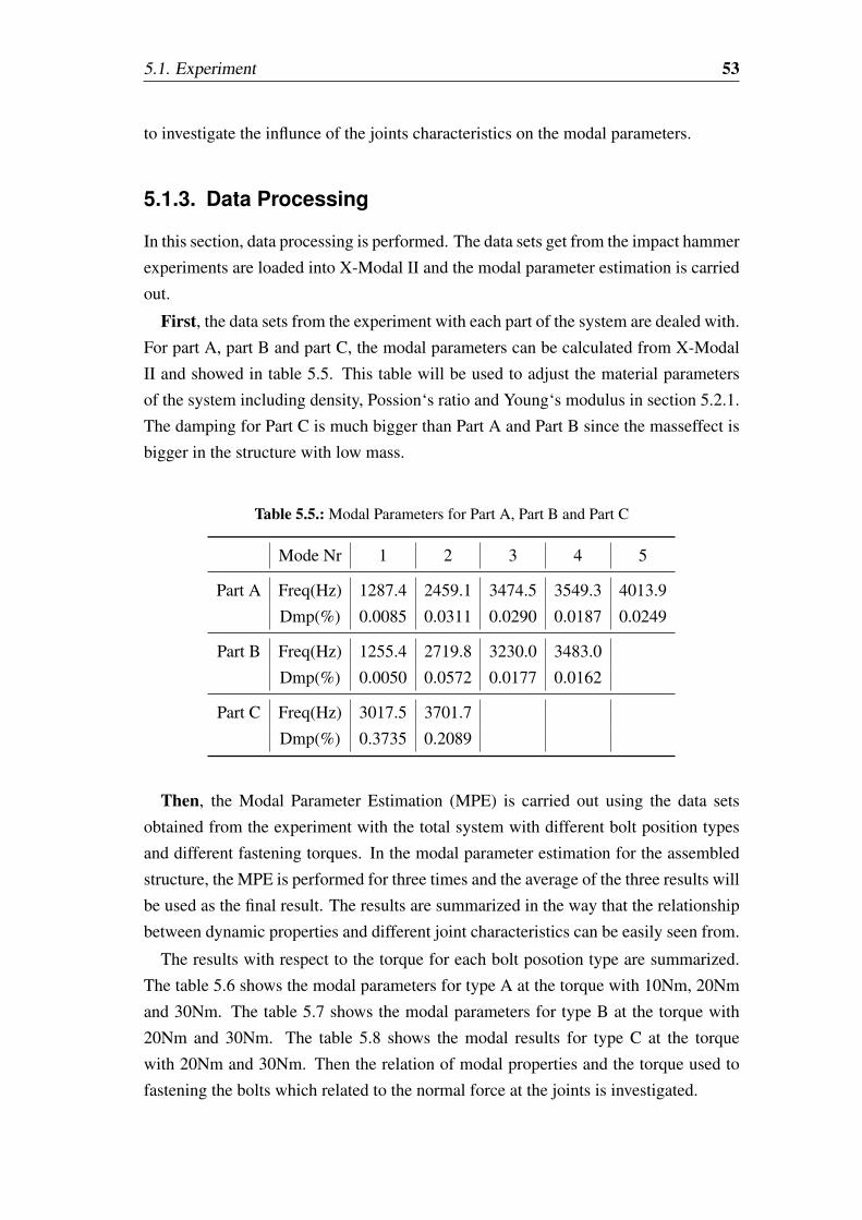
5.1. Experiment 53
to investigate the influnce of the joints characteristics on the modal parameters.
5.1.3. Data Processing
In this section, data processing is performed. The data sets get from the impact hammer
experiments are loaded into X-Modal II and the modal parameter estimation is carried
out.
First, the data sets from the experiment with each part of the system are dealed with.
For part A, part B and part C, the modal parameters can be calculated from X-Modal
II and showed in table 5.5. This table will be used to adjust the material parameters
of the system including density, Possion‘s ratio and Young‘s modulus in section 5.2.1.
The damping for Part C is much bigger than Part A and Part B since the masseffect is
bigger in the structure with low mass.
Table 5.5.: Modal Parameters for Part A, Part B and Part C
Mode Nr 1 2 3 4 5
Part A Freq(Hz) 1287.4 2459.1 3474.5 3549.3 4013.9
Dmp(%) 0.0085 0.0311 0.0290 0.0187 0.0249
Part B Freq(Hz) 1255.4 2719.8 3230.0 3483.0
Dmp(%) 0.0050 0.0572 0.0177 0.0162
Part C Freq(Hz) 3017.5 3701.7
Dmp(%) 0.3735 0.2089
Then, the Modal Parameter Estimation (MPE) is carried out using the data sets
obtained from the experiment with the total system with different bolt position types
and different fastening torques. In the modal parameter estimation for the assembled
structure, the MPE is performed for three times and the average of the three results will
be used as the final result. The results are summarized in the way that the relationship
between dynamic properties and different joint characteristics can be easily seen from.
The results with respect to the torque for each bolt posotion type are summarized.
The table 5.6 shows the modal parameters for type A at the torque with 10Nm, 20Nm
and 30Nm. The table 5.7 shows the modal parameters for type B at the torque with
20Nm and 30Nm. The table 5.8 shows the modal results for type C at the torque
with 20Nm and 30Nm. Then the relation of modal properties and the torque used to
fastening the bolts which related to the normal force at the joints is investigated.
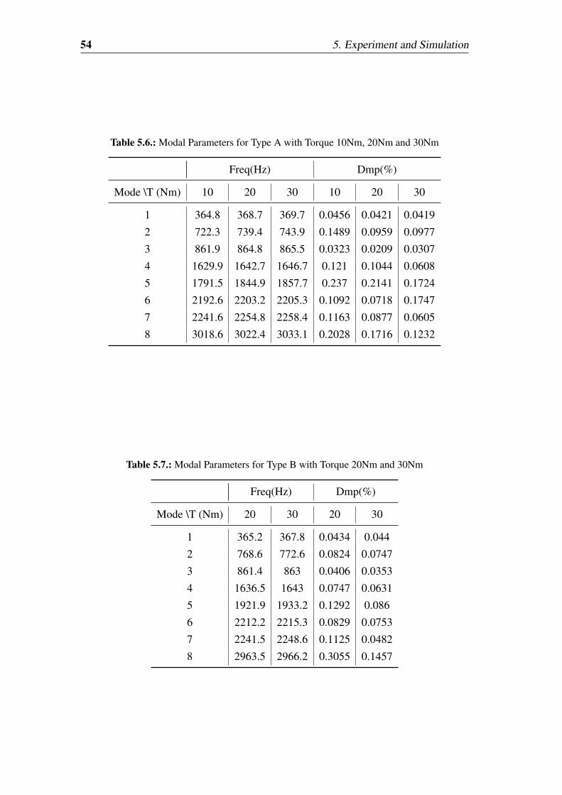
54 5. Experiment and Simulation
Table 5.6.: Modal Parameters for Type A with Torque 10Nm, 20Nm and 30Nm
Freq(Hz) Dmp(%)
Mode \T (Nm) 10 20 30 10 20 30
1 364.8 368.7 369.7 0.0456 0.0421 0.0419
2 722.3 739.4 743.9 0.1489 0.0959 0.0977
3 861.9 864.8 865.5 0.0323 0.0209 0.0307
4 1629.9 1642.7 1646.7 0.121 0.1044 0.0608
5 1791.5 1844.9 1857.7 0.237 0.2141 0.1724
6 2192.6 2203.2 2205.3 0.1092 0.0718 0.1747
7 2241.6 2254.8 2258.4 0.1163 0.0877 0.0605
8 3018.6 3022.4 3033.1 0.2028 0.1716 0.1232
Table 5.7.: Modal Parameters for Type B with Torque 20Nm and 30Nm
Freq(Hz) Dmp(%)
Mode \T (Nm) 20 30 20 30
1 365.2 367.8 0.0434 0.044
2 768.6 772.6 0.0824 0.0747
3 861.4 863 0.0406 0.0353
4 1636.5 1643 0.0747 0.0631
5 1921.9 1933.2 0.1292 0.086
6 2212.2 2215.3 0.0829 0.0753
7 2241.5 2248.6 0.1125 0.0482
8 2963.5 2966.2 0.3055 0.1457
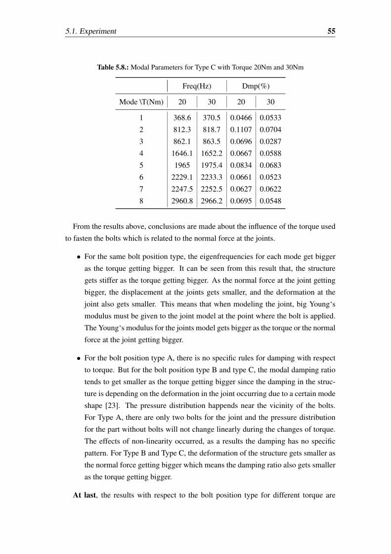
5.1. Experiment 55
Table 5.8.: Modal Parameters for Type C with Torque 20Nm and 30Nm
Freq(Hz) Dmp(%)
Mode \T(Nm) 20 30 20 30
1 368.6 370.5 0.0466 0.0533
2 812.3 818.7 0.1107 0.0704
3 862.1 863.5 0.0696 0.0287
4 1646.1 1652.2 0.0667 0.0588
5 1965 1975.4 0.0834 0.0683
6 2229.1 2233.3 0.0661 0.0523
7 2247.5 2252.5 0.0627 0.0622
8 2960.8 2966.2 0.0695 0.0548
From the results above, conclusions are made about the influence of the torque used
to fasten the bolts which is related to the normal force at the joints.
• For the same bolt position type, the eigenfrequencies for each mode get bigger
as the torque getting bigger. It can be seen from this result that, the structure
gets stiffer as the torque getting bigger. As the normal force at the joint getting
bigger, the displacement at the joints gets smaller, and the deformation at the
joint also gets smaller. This means that when modeling the joint, big Young‘s
modulus must be given to the joint model at the point where the bolt is applied.
The Young‘s modulus for the joints model gets bigger as the torque or the normal
force at the joint getting bigger.
• For the bolt position type A, there is no specific rules for damping with respect
to torque. But for the bolt position type B and type C, the modal damping ratio
tends to get smaller as the torque getting bigger since the damping in the struc-
ture is depending on the deformation in the joint occurring due to a certain mode
shape [23]. The pressure distribution happends near the vicinity of the bolts.
For Type A, there are only two bolts for the joint and the pressure distribution
for the part without bolts will not change linearly during the changes of torque.
The effects of non-linearity occurred, as a results the damping has no specific
pattern. For Type B and Type C, the deformation of the structure gets smaller as
the normal force getting bigger which means the damping ratio also gets smaller
as the torque getting bigger.
At last, the results with respect to the bolt position type for different torque are
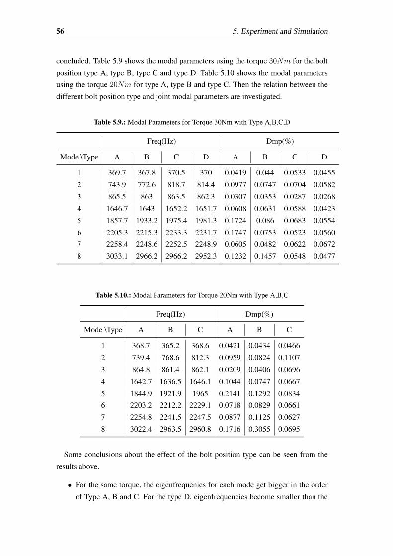
56 5. Experiment and Simulation
concluded. Table 5.9 shows the modal parameters using the torque 30Nm for the bolt
position type A, type B, type C and type D. Table 5.10 shows the modal parameters
using the torque 20Nm for type A, type B and type C. Then the relation between the
different bolt position type and joint modal parameters are investigated.
Table 5.9.: Modal Parameters for Torque 30Nm with Type A,B,C,D
Freq(Hz) Dmp(%)
Mode \Type A B C D A B C D
1 369.7 367.8 370.5 370 0.0419 0.044 0.0533 0.0455
2 743.9 772.6 818.7 814.4 0.0977 0.0747 0.0704 0.0582
3 865.5 863 863.5 862.3 0.0307 0.0353 0.0287 0.0268
4 1646.7 1643 1652.2 1651.7 0.0608 0.0631 0.0588 0.0423
5 1857.7 1933.2 1975.4 1981.3 0.1724 0.086 0.0683 0.0554
6 2205.3 2215.3 2233.3 2231.7 0.1747 0.0753 0.0523 0.0560
7 2258.4 2248.6 2252.5 2248.9 0.0605 0.0482 0.0622 0.0672
8 3033.1 2966.2 2966.2 2952.3 0.1232 0.1457 0.0548 0.0477
Table 5.10.: Modal Parameters for Torque 20Nm with Type A,B,C
Freq(Hz) Dmp(%)
Mode \Type A B C A B C
1 368.7 365.2 368.6 0.0421 0.0434 0.0466
2 739.4 768.6 812.3 0.0959 0.0824 0.1107
3 864.8 861.4 862.1 0.0209 0.0406 0.0696
4 1642.7 1636.5 1646.1 0.1044 0.0747 0.0667
5 1844.9 1921.9 1965 0.2141 0.1292 0.0834
6 2203.2 2212.2 2229.1 0.0718 0.0829 0.0661
7 2254.8 2241.5 2247.5 0.0877 0.1125 0.0627
8 3022.4 2963.5 2960.8 0.1716 0.3055 0.0695
Some conclusions about the effect of the bolt position type can be seen from the
results above.
• For the same torque, the eigenfrequenies for each mode get bigger in the order
of Type A, B and C. For the type D, eigenfrequencies become smaller than the
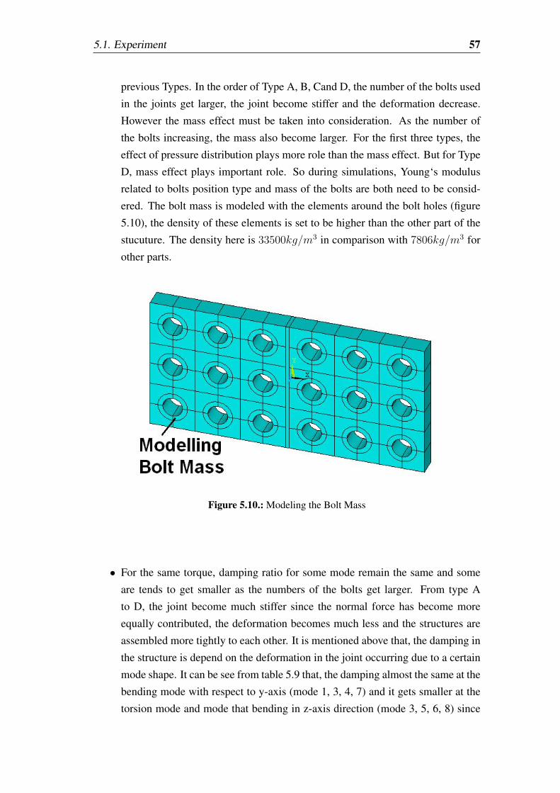
5.1. Experiment 57
previous Types. In the order of Type A, B, Cand D, the number of the bolts used
in the joints get larger, the joint become stiffer and the deformation decrease.
However the mass effect must be taken into consideration. As the number of
the bolts increasing, the mass also become larger. For the first three types, the
effect of pressure distribution plays more role than the mass effect. But for Type
D, mass effect plays important role. So during simulations, Young‘s modulus
related to bolts position type and mass of the bolts are both need to be consid-
ered. The bolt mass is modeled with the elements around the bolt holes (figure
5.10), the density of these elements is set to be higher than the other part of the
stucuture. The density here is 33500kg/m3 in comparison with 7806kg/m3 for
other parts.
Figure 5.10.: Modeling the Bolt Mass
• For the same torque, damping ratio for some mode remain the same and some
are tends to get smaller as the numbers of the bolts get larger. From type A
to D, the joint become much stiffer since the normal force has become more
equally contributed, the deformation becomes much less and the structures are
assembled more tightly to each other. It is mentioned above that, the damping in
the structure is depend on the deformation in the joint occurring due to a certain
mode shape. It can be see from table 5.9 that, the damping almost the same at the
bending mode with respect to y-axis (mode 1, 3, 4, 7) and it gets smaller at the
torsion mode and mode that bending in z-axis direction (mode 3, 5, 6, 8) since
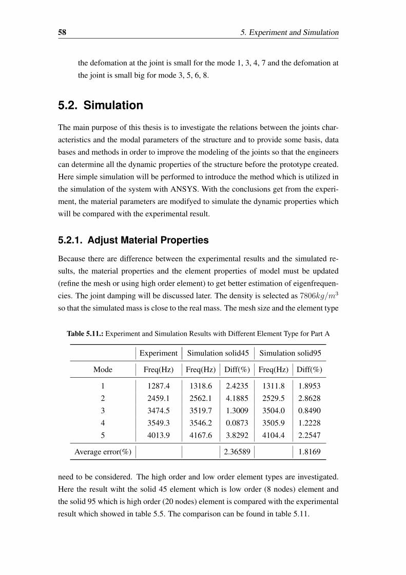
58 5. Experiment and Simulation
the defomation at the joint is small for the mode 1, 3, 4, 7 and the defomation at
the joint is small big for mode 3, 5, 6, 8.
5.2. Simulation
The main purpose of this thesis is to investigate the relations between the joints char-
acteristics and the modal parameters of the structure and to provide some basis, data
bases and methods in order to improve the modeling of the joints so that the engineers
can determine all the dynamic properties of the structure before the prototype created.
Here simple simulation will be performed to introduce the method which is utilized in
the simulation of the system with ANSYS. With the conclusions get from the experi-
ment, the material parameters are modifyed to simulate the dynamic properties which
will be compared with the experimental result.
5.2.1. Adjust Material Properties
Because there are difference between the experimental results and the simulated re-
sults, the material properties and the element properties of model must be updated
(refine the mesh or using high order element) to get better estimation of eigenfrequen-
cies. The joint damping will be discussed later. The density is selected as 7806kg/m3
so that the simulated mass is close to the real mass. The mesh size and the element type
Table 5.11.: Experiment and Simulation Results with Different Element Type for Part A
Experiment Simulation solid45 Simulation solid95
Mode Freq(Hz) Freq(Hz) Diff(%) Freq(Hz) Diff(%)
1 1287.4 1318.6 2.4235 1311.8 1.8953
2 2459.1 2562.1 4.1885 2529.5 2.8628
3 3474.5 3519.7 1.3009 3504.0 0.8490
4 3549.3 3546.2 0.0873 3505.9 1.2228
5 4013.9 4167.6 3.8292 4104.4 2.2547
Average error(%) 2.36589 1.8169
need to be considered. The high order and low order element types are investigated.
Here the result wiht the solid 45 element which is low order (8 nodes) element and
the solid 95 which is high order (20 nodes) element is compared with the experimental
result which showed in table 5.5. The comparison can be found in table 5.11.
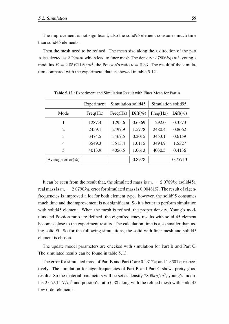
5.2. Simulation 59
The improvement is not significant, also the solid95 element consumes much time
than solid45 elements.
Then the mesh need to be refined. The mesh size along the x direction of the part
A is selected as 2 29mm which lead to finer mesh.The density is 7806kg/m3, young‘s
modulus E = 2 05E11N/m2, the Poisson’s ratio ν = 0 33. The result of the simula-
tion compared with the experimetal data is showed in table 5.12.
Table 5.12.: Experiment and Simulation Result with Finer Mesh for Part A
Experiment Simulation solid45 Simulation solid95
Mode Freq(Hz) Freq(Hz) Diff(%) Freq(Hz) Diff(%)
1 1287.4 1295.6 0.6369 1292.0 0.3573
2 2459.1 2497.9 1.5778 2480.4 0.8662
3 3474.5 3467.5 0.2015 3453.1 0.6159
4 3549.3 3513.4 1.0115 3494.9 1.5327
5 4013.9 4056.5 1.0613 4030.5 0.4136
Average error(%) 0.8978 0.75713
It can be seen from the result that, the simulated mass is ms = 2 0789kg (solid45),
real mass ismr = 2 0790kg, error for simulated mass is 0 00481%. The result of eigen-
frequencies is improved a lot for both element type. however, the solid95 consumes
much time and the improvement is not significant. So it‘s better to perform simulation
with solid45 element. When the mesh is refined, the proper density, Young‘s mod-
ulus and Possion ratio are defined, the eigenfrequency results with solid 45 element
becomes close to the experiment results. The calculation time is also smaller than us-
ing solid95. So for the following simulations, the solid with finer mesh and solid45
element is chosen.
The update model parameters are checked with simulation for Part B and Part C.
The simulated results can be found in table 5.13.
The error for simulated mass of Part B and Part C are 0 2312% and 1 3601% respec-
tively. The simulation for eigenfrequencies of Part B and Part C shows pretty good
results. So the material parameters will be set as density 7806kg/m3, young‘s modu-
lus 2 05E11N/m2 and possion‘s ratio 0 33 along with the refined mesh with soild 45
low order elements.
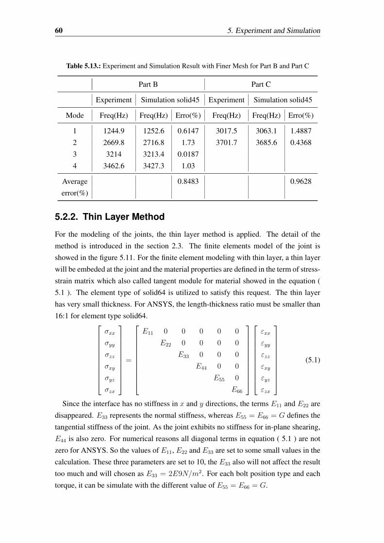
60 5. Experiment and Simulation
Table 5.13.: Experiment and Simulation Result with Finer Mesh for Part B and Part C
Part B Part C
Experiment Simulation solid45 Experiment Simulation solid45
Mode Freq(Hz) Freq(Hz) Erro(%) Freq(Hz) Freq(Hz) Erro(%)
1 1244.9 1252.6 0.6147 3017.5 3063.1 1.4887
2 2669.8 2716.8 1.73 3701.7 3685.6 0.4368
3 3214 3213.4 0.0187
4 3462.6 3427.3 1.03
Average 0.8483 0.9628
error(%)
5.2.2. Thin Layer Method
For the modeling of the joints, the thin layer method is applied. The detail of the
method is introduced in the section 2.3. The finite elements model of the joint is
showed in the figure 5.11. For the finite element modeling with thin layer, a thin layer
will be embeded at the joint and the material properties are defined in the term of stress-
strain matrix which also called tangent module for material showed in the equation (
5.1 ). The element type of solid64 is utilized to satisfy this request. The thin layer
has very small thickness. For ANSYS, the length-thickness ratio must be smaller than
16:1 for element type solid64.
σxx
σyy
σzz
σxy
σyz
σzx
=
E11 0 0 0 0 0
E22 0 0 0 0
E33 0 0 0
E44 0 0
E55 0
E66
εxx
εyy
εzz
εxy
εyz
εzx
(5.1)
Since the interface has no stiffness in x and y directions, the terms E11 and E22 are
disappeared. E33 represents the normal stiffness, whereas E55 = E66 = G defines the
tangential stiffness of the joint. As the joint exhibits no stiffness for in-plane shearing,
E44 is also zero. For numerical reasons all diagonal terms in equation ( 5.1 ) are not
zero for ANSYS. So the values of E11, E22 and E33 are set to some small values in the
calculation. These three parameters are set to 10, the E33 also will not affect the result
too much and will chosen as E33 = 2E9N/m2. For each bolt position type and each
torque, it can be simulate with the different value of E55 = E66 = G.
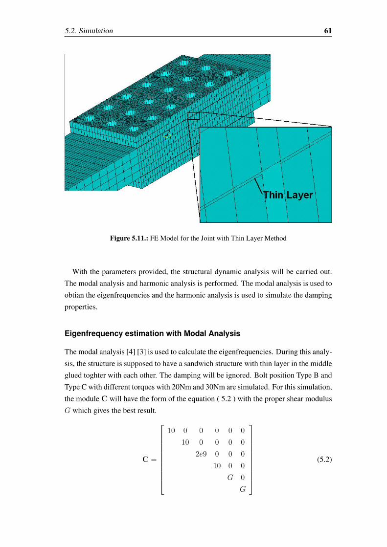
5.2. Simulation 61
Figure 5.11.: FE Model for the Joint with Thin Layer Method
With the parameters provided, the structural dynamic analysis will be carried out.
The modal analysis and harmonic analysis is performed. The modal analysis is used to
obtian the eigenfrequencies and the harmonic analysis is used to simulate the damping
properties.
Eigenfrequency estimation with Modal Analysis
The modal analysis [4] [3] is used to calculate the eigenfrequencies. During this analy-
sis, the structure is supposed to have a sandwich structure with thin layer in the middle
glued toghter with each other. The damping will be ignored. Bolt position Type B and
Type C with different torques with 20Nm and 30Nm are simulated. For this simulation,
the module C will have the form of the equation ( 5.2 ) with the proper shear modulus
G which gives the best result.
C =
10 0 0 0 0 0
10 0 0 0 0
2e9 0 0 0
10 0 0
G 0
G
(5.2)
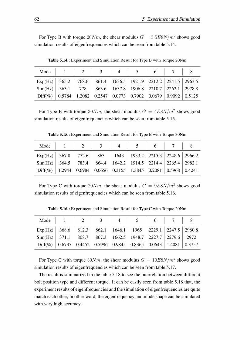
62 5. Experiment and Simulation
For Type B with torque 20Nm, the shear modulus G = 3 5E8N/m2 shows good
simulation results of eigenfrequencies which can be seen from table 5.14.
Table 5.14.: Experiment and Simulation Result for Type B with Torque 20Nm
Mode 1 2 3 4 5 6 7 8
Exp(Hz) 365.2 768.6 861.4 1636.5 1921.9 2212.2 2241.5 2963.5
Sim(Hz) 363.1 778 863.6 1637.8 1906.8 2210.7 2262.1 2978.8
Diff(%) 0.5784 1.2082 0.2547 0.0773 0.7902 0.0679 0.9092 0.5125
For Type B with torque 30Nm, the shear modulus G = 4E8N/m2 shows good
simulation results of eigenfrequencies which can be seen from table 5.15.
Table 5.15.: Experiment and Simulation Result for Type B with Torque 30Nm
Mode 1 2 3 4 5 6 7 8
Exp(Hz) 367.8 772.6 863 1643 1933.2 2215.3 2248.6 2966.2
Sim(Hz) 364.5 783.4 864.4 1642.2 1914.5 2214.4 2265.4 2982.1
Diff(%) 1.2944 0.6984 0.0656 0.3155 1.3845 0.2081 0.5968 0.4241
For Type C with torque 20Nm, the shear modulus G = 9E8N/m2 shows good
simulation results of eigenfrequencies which can be seen from table 5.16.
Table 5.16.: Experiment and Simulation Result for Type C with Torque 20Nm
Mode 1 2 3 4 5 6 7 8
Exp(Hz) 368.6 812.3 862.1 1646.1 1965 2229.1 2247.5 2960.8
Sim(Hz) 371.1 808.7 867.3 1662.5 1948.7 2227.7 2279.6 2972
Diff(%) 0.6737 0.4452 0.5996 0.9845 0.8365 0.0643 1.4081 0.3757
For Type C with torque 30Nm, the shear modulus G = 10E8N/m2 shows good
simulation results of eigenfrequencies which can be seen from table 5.17.
The result is summarized in the table 5.18 to see the interrelation between different
bolt position type and different torque. It can be easily seen from table 5.18 that, the
experiment results of eigenfrequencies and the simulation of eigenfrequencies are quite
match each other, in other word, the eigenfrequency and mode shape can be simulated
with very high accuracy.
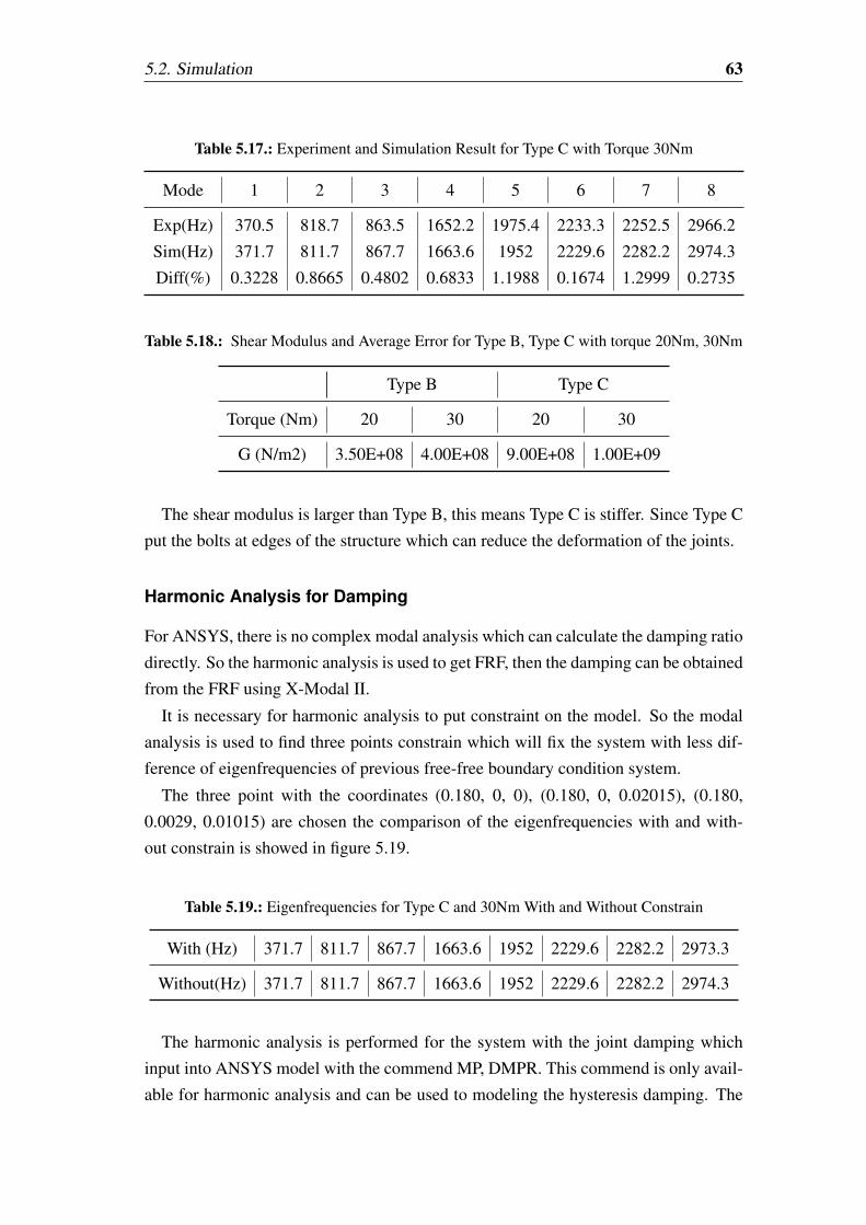
5.2. Simulation 63
Table 5.17.: Experiment and Simulation Result for Type C with Torque 30Nm
Mode 1 2 3 4 5 6 7 8
Exp(Hz) 370.5 818.7 863.5 1652.2 1975.4 2233.3 2252.5 2966.2
Sim(Hz) 371.7 811.7 867.7 1663.6 1952 2229.6 2282.2 2974.3
Diff(%) 0.3228 0.8665 0.4802 0.6833 1.1988 0.1674 1.2999 0.2735
Table 5.18.: Shear Modulus and Average Error for Type B, Type C with torque 20Nm, 30Nm
Type B Type C
Torque (Nm) 20 30 20 30
G (N/m2) 3.50E+08 4.00E+08 9.00E+08 1.00E+09
The shear modulus is larger than Type B, this means Type C is stiffer. Since Type C
put the bolts at edges of the structure which can reduce the deformation of the joints.
Harmonic Analysis for Damping
For ANSYS, there is no complex modal analysis which can calculate the damping ratio
directly. So the harmonic analysis is used to get FRF, then the damping can be obtained
from the FRF using X-Modal II.
It is necessary for harmonic analysis to put constraint on the model. So the modal
analysis is used to find three points constrain which will fix the system with less dif-
ference of eigenfrequencies of previous free-free boundary condition system.
The three point with the coordinates (0.180, 0, 0), (0.180, 0, 0.02015), (0.180,
0.0029, 0.01015) are chosen the comparison of the eigenfrequencies with and with-
out constrain is showed in figure 5.19.
Table 5.19.: Eigenfrequencies for Type C and 30Nm With and Without Constrain
With (Hz) 371.7 811.7 867.7 1663.6 1952 2229.6 2282.2 2973.3
Without(Hz) 371.7 811.7 867.7 1663.6 1952 2229.6 2282.2 2974.3
The harmonic analysis is performed for the system with the joint damping which
input into ANSYS model with the commend MP, DMPR. This commend is only avail-
able for harmonic analysis and can be used to modeling the hysteresis damping. The
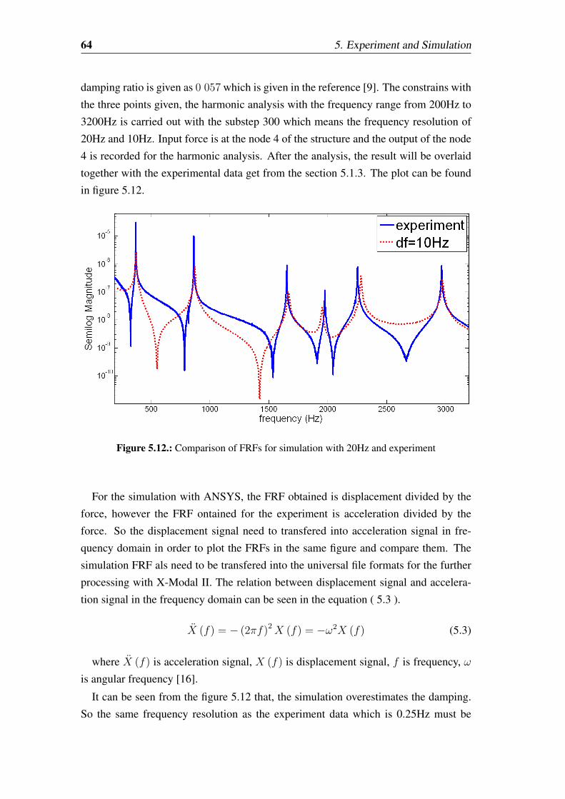
64 5. Experiment and Simulation
damping ratio is given as 0 057 which is given in the reference [9]. The constrains with
the three points given, the harmonic analysis with the frequency range from 200Hz to
3200Hz is carried out with the substep 300 which means the frequency resolution of
20Hz and 10Hz. Input force is at the node 4 of the structure and the output of the node
4 is recorded for the harmonic analysis. After the analysis, the result will be overlaid
together with the experimental data get from the section 5.1.3. The plot can be found
in figure 5.12.
Figure 5.12.: Comparison of FRFs for simulation with 20Hz and experiment
For the simulation with ANSYS, the FRF obtained is displacement divided by the
force, however the FRF ontained for the experiment is acceleration divided by the
force. So the displacement signal need to transfered into acceleration signal in fre-
quency domain in order to plot the FRFs in the same figure and compare them. The
simulation FRF als need to be transfered into the universal file formats for the further
processing with X-Modal II. The relation between displacement signal and accelera-
tion signal in the frequency domain can be seen in the equation ( 5.3 ).
X (f) = − (2πf)2X (f) = −ω2X (f) (5.3)
where X (f) is acceleration signal, X (f) is displacement signal, f is frequency, ω
is angular frequency [16].
It can be seen from the figure 5.12 that, the simulation overestimates the damping.
So the same frequency resolution as the experiment data which is 0.25Hz must be
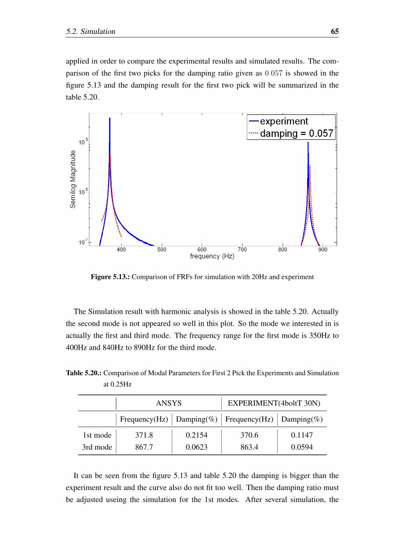
5.2. Simulation 65
applied in order to compare the experimental results and simulated results. The com-
parison of the first two picks for the damping ratio given as 0 057 is showed in the
figure 5.13 and the damping result for the first two pick will be summarized in the
table 5.20.
Figure 5.13.: Comparison of FRFs for simulation with 20Hz and experiment
The Simulation result with harmonic analysis is showed in the table 5.20. Actually
the second mode is not appeared so well in this plot. So the mode we interested in is
actually the first and third mode. The frequency range for the first mode is 350Hz to
400Hz and 840Hz to 890Hz for the third mode.
Table 5.20.: Comparison of Modal Parameters for First 2 Pick the Experiments and Simulation
at 0.25Hz
ANSYS EXPERIMENT(4boltT 30N)
Frequency(Hz) Damping(%) Frequency(Hz) Damping(%)
1st mode 371.8 0.2154 370.6 0.1147
3rd mode 867.7 0.0623 863.4 0.0594
It can be seen from the figure 5.13 and table 5.20 the damping is bigger than the
experiment result and the curve also do not fit too well. Then the damping ratio must
be adjusted useing the simulation for the 1st modes. After several simulation, the
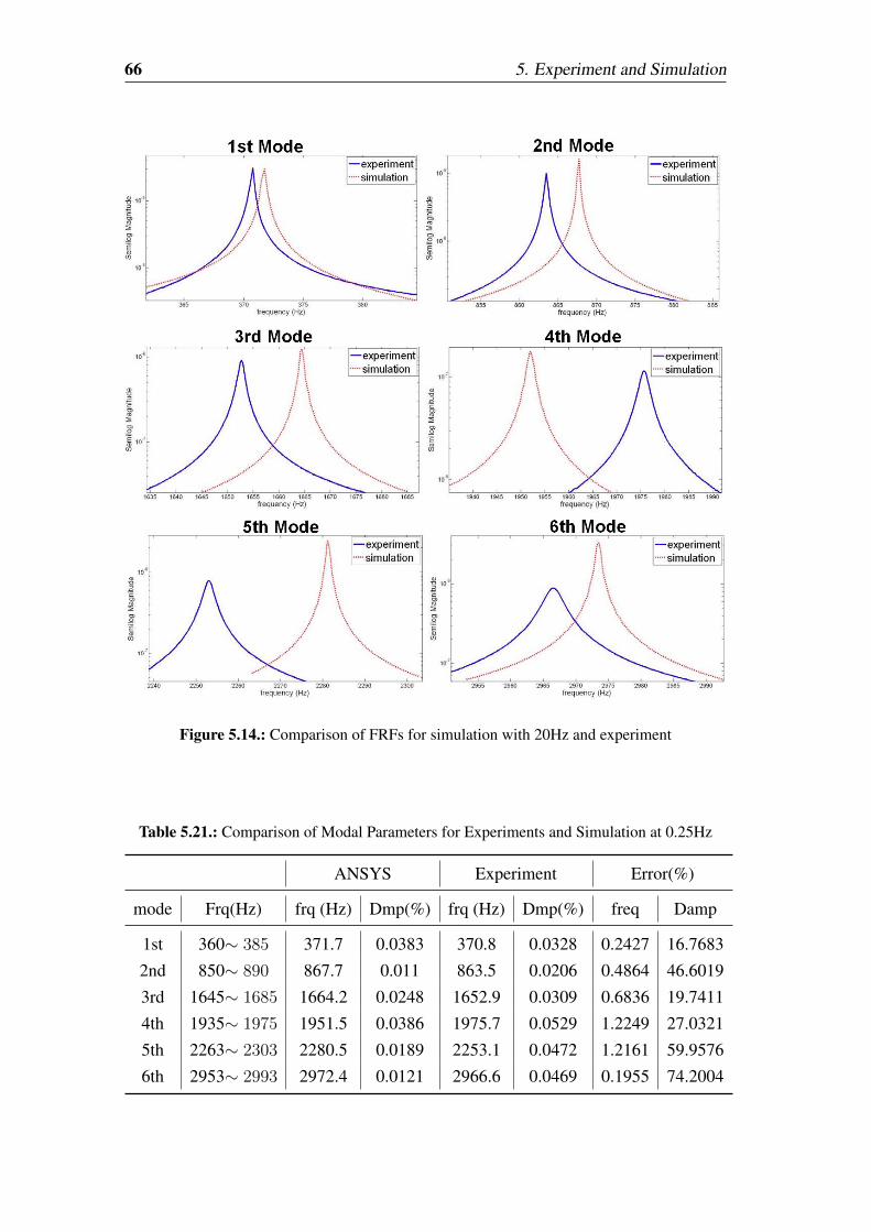
66 5. Experiment and Simulation
Figure 5.14.: Comparison of FRFs for simulation with 20Hz and experiment
Table 5.21.: Comparison of Modal Parameters for Experiments and Simulation at 0.25Hz
ANSYS Experiment Error(%)
mode Frq(Hz) frq (Hz) Dmp(%) frq (Hz) Dmp(%) freq Damp
1st 360∼ 385 371.7 0.0383 370.8 0.0328 0.2427 16.7683
2nd 850∼ 890 867.7 0.011 863.5 0.0206 0.4864 46.6019
3rd 1645∼ 1685 1664.2 0.0248 1652.9 0.0309 0.6836 19.7411
4th 1935∼ 1975 1951.5 0.0386 1975.7 0.0529 1.2249 27.0321
5th 2263∼ 2303 2280.5 0.0189 2253.1 0.0472 1.2161 59.9576
6th 2953∼ 2993 2972.4 0.0121 2966.6 0.0469 0.1955 74.2004

5.2. Simulation 67
damping ratio is updated to 0.01 which give the best curve fit to the experiment result.
The simulation result is showed in figure 5.14 and table 5.21.
It can be seen from the figure 5.14 and table 5.21 that, the estimation of damping
is not so good. the highest error for damping is 74%. The simulation showes good
estimation for the first three mode and get worse for the mode in high frequency range.
the result can be improved with using the material damping also with the constant
frequency independent stiffness matrix coefficient βξj .

6. Conclusions andRecommendations
In this thesis, the structures with multiple joint characteristics are designed, constructed
and investigated . The structures which satisfies the criteria is manufactured and used
in the investigation of the system with multiple joint characteristics. Analytical ap-
proach is performed in order to select the modal parameter estimation methods. The
experimental approach summarizes the influence caused by the different bolts posi-
tion and the different torque, the influence is discussed with respect to not only the
eigenfrequencies but also damping ratio. the simulation is performed to compare the
simulated results with experimental results. In this Chapter several conclusions are
made and some recommendations for further work are given.
6.1. Conclusions
• The PTD method showed best results for the analytical data with low damping,
the PTD method is utilized to the analysis with the experimental data. The PTD
method is high order time domain method. As time domain methods tend to
provide the best results when a large frequency ranges and high order methods
require more spatial data because they use only a limited subset of spatial data.
For our structure the frequency range will be 0 3000Hz and also the system use
only 2 accelerometers which means there are few physical DOFs.
• For the same bolt position (identical pressure distribution), the eigenfrequencies
for each mode will get bigger as the torque getting bigger. As the normal force
at the joint getting bigger, the deformation at the joint gets smaller, the system
gets stiffer which means young‘s modulus for the joint model get bigger.
• For the same bolt position (identical pressure distribution), modal damping ra-
tios tend to get smaller as the torque getting bigger, since the damping in the
structure is also dependent on the deformation in the joint occurring due to a
certain mode shape. Damping ratios also get smaller as the torque get smaller.
70 6. Conclusions and Recommendations
Type A performs non-linearity which implies that, there must be enough bolts to
make the structure perform linear.
• For the same torque, according to the order of the type A, B and C, the eigen-
frequenies for each mode get bigger. But for the type D the eigenfrequency has
become smaller than the previous bolt position type. In the order of type A, B, C,
D, the number of the bolts used in the joints will get larger, the joint will become
more and stiffer and the deformation will decrease. At the same time, the mass
effect for the simulation must also take place. If the strucutre can be designed
more heavier, this effect will be avoided.
• For the same torque, the damping ratio for the most modes also tends get smaller
according to the order of the type A, B, C and D, which means that the numbers
of the bolts get larger and the pressure get more well-distributed. From type A
to D, the joint become much stiffer; the normal force has become more equally
distributed; and the deformation becomes much less.
• The eigenfrequencies and the mode shapes can be calculated with finite elements
method high accuracy. In this thesis, thin layer elements method is utilized and
this method can simulate not only the different type of bolt position, but also the
different torque used to fastening the bolts (pressure distribution).
• The damping ratio can also be simulated with finite element method. However,
the result still shows big errors since the damping is very sensitive.
6.2. Recommendations
• For the structure used in the experiments, we only performed with part B and
part C. In the further work the part A must also be utilized to perform more
complicated structures with different joint characteristics. The structure is better
to be more heavier, in order to avoid the massloading effect.
• More complex structure can be constructed with the Part A, Part B and Part C to
investigate the system with joint characteristics.
• For the analytical approach, the noise must be take consider with respect to
power, amplitude and so on. Also the model must be generated both in the
time domain and frequency domain in order to check the effect of data sets with
different domain to the MPE methods.
6.2. Recommendations 71
• For the experiment, the shaker can be used instead of the impact hammer in
further work, by the reason that the impact hammer cannot provide the structure
with constant impulse. The shaker can solve this problem easily. But for this
method, the massloading effect of the accelerometers will be need to take in
consider.
• For the experiment, instead of use the FRF signal of the system, the impulse
signal can be directly used in order to investigate the MPE methods with the
experimental data sets in time domain.
• For the simulation, the stiffness and damping property are considered as constant
in the thin layer at the joint. But in further work, the material and dynamic
properties of system must be determined differently from position to position in
the thin layer elements according to the bolt position. This must be providing
much better result.
• For simulation, ANSYS is used to perform the simulation, where the length to
thickness ratio of the thin layer for solid 64 is smaller than 16:1. So other element
type or other software such as Nastran which allows bigger length to thickness
ratio must be applied for simulation.
• As a consequence, investigattion of the effect of the thickness ratio of the thin
layer and the elements nearby is required.
• For the simulation, modeling the bolts with different methods will be also one
of the interesting research fields for the further work, which can be referenced
from referece [13]
• For damping, more investigations are required.

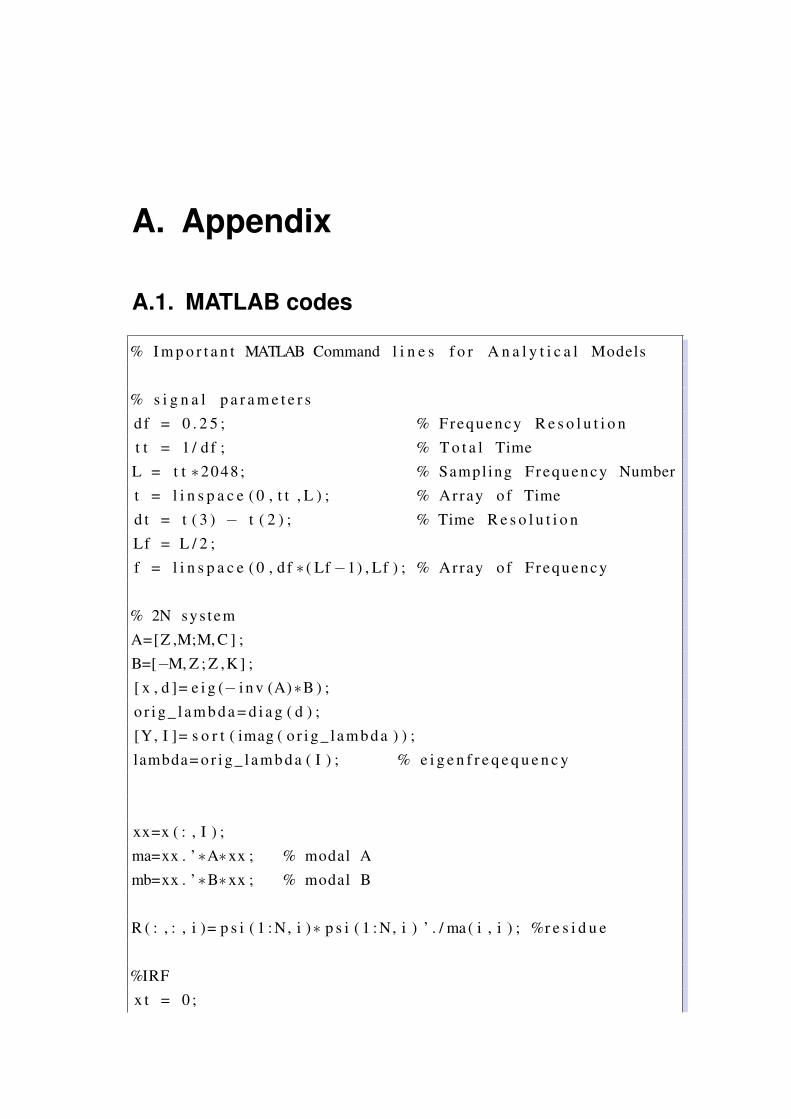
A. Appendix
A.1. MATLAB codes
% I m p o r t a n t MATLAB Command l i n e s f o r A n a l y t i c a l Models
% s i g n a l p a r a m e t e r s
d f = 0 . 2 5 ; % Frequency R e s o l u t i o n
t t = 1 / d f ; % T o t a l Time
L = t t ∗2048 ; % Sampl ing Frequency Number
t = l i n s p a c e ( 0 , t t , L ) ; % Array of Time
d t = t ( 3 ) − t ( 2 ) ; % Time R e s o l u t i o n
Lf = L / 2 ;
f = l i n s p a c e ( 0 , d f ∗ ( Lf−1) , Lf ) ; % Array of Frequency
% 2N sys tem
A=[Z ,M;M, C ] ;
B=[−M, Z ; Z ,K ] ;
[ x , d ]= e i g (− i n v (A)∗B ) ;
o r i g _ l a m b d a = d i a g ( d ) ;
[Y, I ]= s o r t ( imag ( o r i g _ l a m b d a ) ) ;
lambda= o r i g _ l a m b d a ( I ) ; % e i g e n f r e q e q u e n c y
xx=x ( : , I ) ;
ma=xx . ’∗A∗xx ; % modal A
mb=xx . ’∗B∗xx ; % modal B
R ( : , : , i )= p s i ( 1 : N, i )∗ p s i ( 1 : N, i ) ’ . / ma ( i , i ) ; %r e s i d u e
%IRF
x t = 0 ;
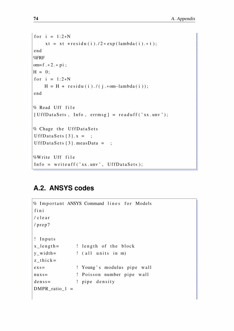
74 A. Appendix
f o r i = 1 :2∗N
x t = x t + r e s i d u ( i ) . / 2 ∗ exp ( lambda ( i ) . ∗ t ) ;
end
%FRF
om= f . ∗ 2 . ∗ p i ;
H = 0 ;
f o r i = 1 :2∗N
H = H + r e s i d u ( i ) . / ( j . ∗om−lambda ( i ) ) ;
end
% Read Uff f i l e
[ U f f D a t a S e t s , In fo , e r rmsg ] = r e a d u f f ( ’ xx . unv ’ ) ;
% Chage t h e U f f D a t a S e t s
U f f D a t a S e t s 3 . x = ;
U f f D a t a S e t s 3 . measData = ;
%Wri t e Uff f i l e
I n f o = w r i t e u f f ( ’ xx . unv ’ , U f f D a t a S e t s ) ;
A.2. ANSYS codes
% I m p o r t a n t ANSYS Command l i n e s f o r Models
f i n i
/ c l e a r
/ p rep7
! I n p u t s
x _ l e n g t h = ! l e n g t h o f t h e b l o c k
y_wid th = ! ( a l l u n i t s i n m)
z _ t h i c k =
exs = ! Young ’ s modulus p i p e w a l l
nuxs= ! P o i s s o n number p i p e w a l l
d e n s s = ! p i p e d e n s i t y
DMPR_ratio_1 =
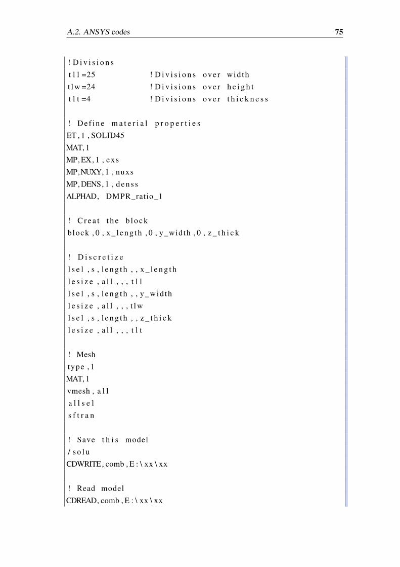
A.2. ANSYS codes 75
! D i v i s i o n s
t l l =25 ! D i v i s i o n s ove r wid th
t l w =24 ! D i v i s i o n s ove r h e i g h t
t l t =4 ! D i v i s i o n s ove r t h i c k n e s s
! D e f in e m a t e r i a l p r o p e r t i e s
ET , 1 , SOLID45
MAT, 1
MP, EX, 1 , exs
MP,NUXY, 1 , nuxs
MP, DENS, 1 , d e n s s
ALPHAD, DMPR_ratio_1
! C r e a t t h e b l o c k
block , 0 , x _ l e n g t h , 0 , y_width , 0 , z _ t h i c k
! D i s c r e t i z e
l s e l , s , l e n g t h , , x _ l e n g t h
l e s i z e , a l l , , , t l l
l s e l , s , l e n g t h , , y_wid th
l e s i z e , a l l , , , t l w
l s e l , s , l e n g t h , , z _ t h i c k
l e s i z e , a l l , , , t l t
! Mesh
type , 1
MAT, 1
vmesh , a l l
a l l s e l
s f t r a n
! Save t h i s model
/ s o l u
CDWRITE, comb , E : \ xx \ xx
! Read model
CDREAD, comb , E : \ xx \ xx
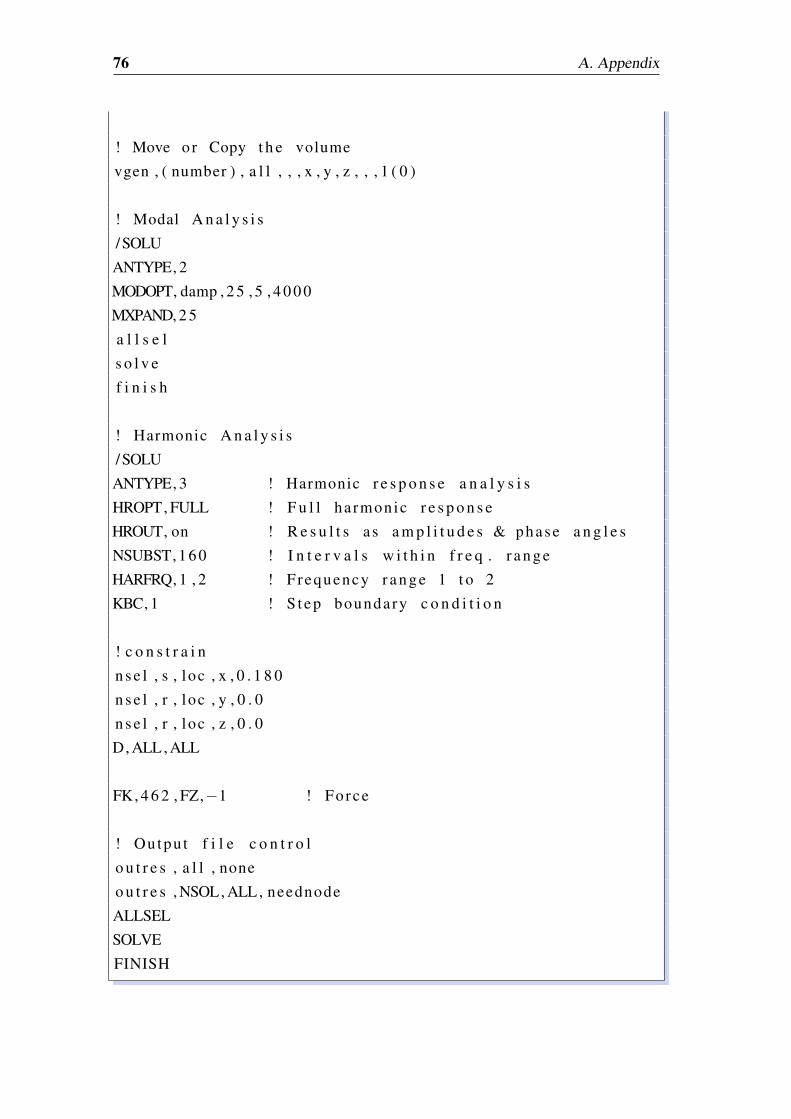
76 A. Appendix
! Move or Copy t h e volume
vgen , ( number ) , a l l , , , x , y , z , , , 1 ( 0 )
! Modal A n a l y s i s
/SOLU
ANTYPE, 2
MODOPT, damp , 2 5 , 5 , 4 0 0 0
MXPAND, 2 5
a l l s e l
s o l v e
f i n i s h
! Harmonic A n a l y s i s
/SOLU
ANTYPE, 3 ! Harmonic r e s p o n s e a n a l y s i s
HROPT, FULL ! F u l l harmonic r e s p o n s e
HROUT, on ! R e s u l t s a s a m p l i t u d e s & phase a n g l e s
NSUBST, 1 6 0 ! I n t e r v a l s w i t h i n f r e q . r a n g e
HARFRQ, 1 , 2 ! Frequency r a n g e 1 t o 2
KBC, 1 ! S t ep boundary c o n d i t i o n
! c o n s t r a i n
n s e l , s , loc , x , 0 . 1 8 0
n s e l , r , loc , y , 0 . 0
n s e l , r , loc , z , 0 . 0
D, ALL, ALL
FK, 4 6 2 , FZ,−1 ! Force
! Outpu t f i l e c o n t r o l
o u t r e s , a l l , none
o u t r e s , NSOL, ALL, neednode
ALLSEL
SOLVE
FINISH

A.3. Blueprint 77
A.3. Blueprint
Figure A.1.: Drawing of the structure A
For the further work, structure A must be utilized. and it can constructed to the
structure showed in figure A.4.

78 A. Appendix
Figure A.2.: Drawing of the structure B
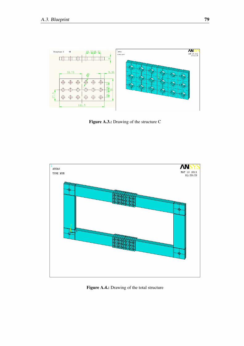
A.3. Blueprint 79
Figure A.3.: Drawing of the structure C
Figure A.4.: Drawing of the total structure

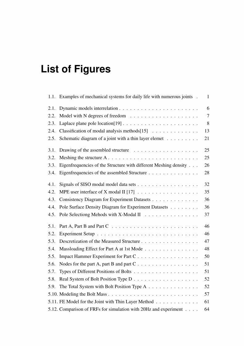
List of Figures
1.1. Examples of mechanical systems for daily life with numerous joints . 1
2.1. Dynamic models interrelation . . . . . . . . . . . . . . . . . . . . . . 6
2.2. Model with N degrees of freedom . . . . . . . . . . . . . . . . . . . 7
2.3. Laplace plane pole location[19] . . . . . . . . . . . . . . . . . . . . . 8
2.4. Classification of modal analysis methods[15] . . . . . . . . . . . . . 13
2.5. Schematic diagram of a joint with a thin layer elemet . . . . . . . . . 21
3.1. Drawing of the assembled structure . . . . . . . . . . . . . . . . . . 25
3.2. Meshing the structure A . . . . . . . . . . . . . . . . . . . . . . . . . 25
3.3. Eigenfrequencies of the Structure with different Meshing density . . . 26
3.4. Eigenfrequencies of the assembled Structure . . . . . . . . . . . . . . 28
4.1. Signals of SISO modal model data sets . . . . . . . . . . . . . . . . . 32
4.2. MPE user interface of X modal II [17] . . . . . . . . . . . . . . . . . 35
4.3. Consistency Diagram for Experiment Datasets . . . . . . . . . . . . . 36
4.4. Pole Surface Density Diagram for Experiment Datasets . . . . . . . . 36
4.5. Pole Selectiong Mehods with X-Modal II . . . . . . . . . . . . . . . 37
5.1. Part A, Part B and Part C . . . . . . . . . . . . . . . . . . . . . . . . 46
5.2. Experiment Setup . . . . . . . . . . . . . . . . . . . . . . . . . . . . 46
5.3. Descretization of the Measured Structure . . . . . . . . . . . . . . . . 47
5.4. Massloading Effect for Part A at 1st Mode . . . . . . . . . . . . . . . 48
5.5. Impact Hammer Experiment for Part C . . . . . . . . . . . . . . . . . 50
5.6. Nodes for the part A, part B and part C . . . . . . . . . . . . . . . . . 51
5.7. Types of Different Positions of Bolts . . . . . . . . . . . . . . . . . . 51
5.8. Real System of Bolt Position Type D . . . . . . . . . . . . . . . . . . 52
5.9. The Total System with Bolt Position Type A . . . . . . . . . . . . . . 52
5.10. Modeling the Bolt Mass . . . . . . . . . . . . . . . . . . . . . . . . . 57
5.11. FE Model for the Joint with Thin Layer Method . . . . . . . . . . . . 61
5.12. Comparison of FRFs for simulation with 20Hz and experiment . . . . 64

82 List of Figures
5.13. Comparison of FRFs for simulation with 20Hz and experiment . . . . 65
5.14. Comparison of FRFs for simulation with 20Hz and experiment . . . . 66
A.1. Drawing of the structure A . . . . . . . . . . . . . . . . . . . . . . . 77
A.2. Drawing of the structure B . . . . . . . . . . . . . . . . . . . . . . . 78
A.3. Drawing of the structure C . . . . . . . . . . . . . . . . . . . . . . . 79
A.4. Drawing of the total structure . . . . . . . . . . . . . . . . . . . . . . 79
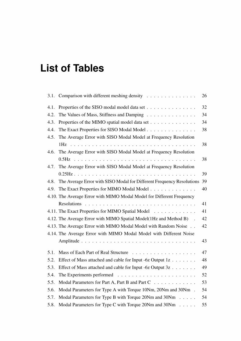
List of Tables
3.1. Comparison with different meshing density . . . . . . . . . . . . . . 26
4.1. Properties of the SISO modal model data set . . . . . . . . . . . . . . 32
4.2. The Values of Mass, Stiffness and Damping . . . . . . . . . . . . . . 34
4.3. Properties of the MIMO spatial model data set . . . . . . . . . . . . . 34
4.4. The Exact Properties for SISO Modal Model . . . . . . . . . . . . . . 38
4.5. The Average Error with SISO Modal Model at Frequency Resolution
1Hz . . . . . . . . . . . . . . . . . . . . . . . . . . . . . . . . . . . 38
4.6. The Average Error with SISO Modal Model at Frequency Resolution
0.5Hz . . . . . . . . . . . . . . . . . . . . . . . . . . . . . . . . . . 38
4.7. The Average Error with SISO Modal Model at Frequency Resolution
0.25Hz . . . . . . . . . . . . . . . . . . . . . . . . . . . . . . . . . . 39
4.8. The Average Error with SISO Modal for Different Frequency Resolutions 39
4.9. The Exact Properties for MIMO Modal Model . . . . . . . . . . . . . 40
4.10. The Average Error with MIMO Modal Model for Different Frequency
Resolutions . . . . . . . . . . . . . . . . . . . . . . . . . . . . . . . 41
4.11. The Exact Properties for MIMO Spatial Model . . . . . . . . . . . . 41
4.12. The Average Error with MIMO Spatial Model(1Hz and Method B) . 42
4.13. The Average Error with MIMO Modal Model with Random Noise . . 42
4.14. The Average Error with MIMO Modal Model with Different Noise
Amplitude . . . . . . . . . . . . . . . . . . . . . . . . . . . . . . . . 43
5.1. Mass of Each Part of Real Structure . . . . . . . . . . . . . . . . . . 47
5.2. Effect of Mass attached and cable for Input -6z Output 1z . . . . . . . 48
5.3. Effect of Mass attached and cable for Input -6z Output 3z . . . . . . . 49
5.4. The Experiments performed . . . . . . . . . . . . . . . . . . . . . . 52
5.5. Modal Parameters for Part A, Part B and Part C . . . . . . . . . . . . 53
5.6. Modal Parameters for Type A with Torque 10Nm, 20Nm and 30Nm . 54
5.7. Modal Parameters for Type B with Torque 20Nm and 30Nm . . . . . 54
5.8. Modal Parameters for Type C with Torque 20Nm and 30Nm . . . . . 55
84 List of Tables
5.9. Modal Parameters for Torque 30Nm with Type A,B,C,D . . . . . . . 56
5.10. Modal Parameters for Torque 20Nm with Type A,B,C . . . . . . . . . 56
5.11. Experiment and Simulation Results with Different Element Type for
Part A . . . . . . . . . . . . . . . . . . . . . . . . . . . . . . . . . . 58
5.12. Experiment and Simulation Result with Finer Mesh for Part A . . . . 59
5.13. Experiment and Simulation Result with Finer Mesh for Part B and Part C 60
5.14. Experiment and Simulation Result for Type B with Torque 20Nm . . 62
5.15. Experiment and Simulation Result for Type B with Torque 30Nm . . 62
5.16. Experiment and Simulation Result for Type C with Torque 20Nm . . 62
5.17. Experiment and Simulation Result for Type C with Torque 30Nm . . 63
5.18. Shear Modulus and Average Error for Type B, Type C with torque
20Nm, 30Nm . . . . . . . . . . . . . . . . . . . . . . . . . . . . . . 63
5.19. Eigenfrequencies for Type C and 30Nm With and Without Constrain . 63
5.20. Comparison of Modal Parameters for First 2 Pick the Experiments and
Simulation at 0.25Hz . . . . . . . . . . . . . . . . . . . . . . . . . . 65
5.21. Comparison of Modal Parameters for Experiments and Simulation at
0.25Hz . . . . . . . . . . . . . . . . . . . . . . . . . . . . . . . . . . 66

Bibliography
[1] Douglas E. Adams. Modal parameter estimation report. Technical report, Uni-
versity of Cincinnati Structural Dynamics Research Laboratory, 01 1998.
[2] Cyril M. Harris Allan G. Piersol, Thomas L. Paez. Harris’ shock and vibra-
tion handbook. ISBN 0071508198, 9780071508193. McGraw Hill Professional,
2009.
[3] Inc. ANSYS. Ansys structural analysis guide ansys release 9.0. Technical report,
ANSYS, Inc., 11 2004.
[4] ANSYS, Inc. ANSYS 11.0 Reference, 2007.
[5] D.L. Brown A.W.Phillips, R.J. Allemang. Autonomous modal parameter esti-
mation: Methodology. Technical report, Structural Dynamics Research Labora-
tory,University of Cincinnati, Cincinnati, OH 45221-0072 USA.
[6] Primoz Cermelj. UFF File Reading and Writing. MATLAB Center,
http://www.mathworks.com/matlabcentral/fileexchange/6395-uff-file-reading-
and-writing, 02 2011.
[7] T. N. Hatzigogos D.A. Karampatakis. A model to describe creeping behavior of
thin-layer element for interfaces and joints. Technical report, Laboratory of Soil
Mechanics and Foundations, Aristotle University of Thessaloniki.
[8] Jeffrey L. Dohner. On the development of methodologies for constructing pre-
dictive models of structures with joints and interfaces. Technical report, The
Structural Dynamics Department, Sandia National Laboratories, 2000.
[9] S. Bograd et al. Modeling the dynamics of mechanical joints. Mechanical Sys-
tems and Signal Processing, 2011.
[10] Angel Moises Iglesias. Investigating various modal analysis extraction tech-
niques to estimate damping ratio. Master’s thesis, Virginia Polytechnic Institute
and State University, 06 2000.
86 Bibliography
[11] Sheldon Imaoka. Addendum to structural damping. Technical report, ANSYS.net
Tips and Tricks, 04 2008.
[12] LMS Inc. Lms polymax - a revolution in modal parameter estimation.
[13] Beom-Soo Kang Jeong Kim, Joo-Cheol Yoon. Finite element analysis and mod-
eling of structure with bolted joints. Applied Mathematical Modelling, 31:895–
911, 2007.
[14] LMS international. Enhanced Exploitation of Vibration Test Data by the Poly-
max Modal Parameter Estimation Method, Proceddings of the 5th International
Symposium on Enviromental Testing for Space Programmes. European Space
Agency, 08 2004.
[15] Maia and Silva et al. Theoretical and Experimental Modal Analysis. Research
Studies Press LTD, Baldock, Herfordshire, England, 1998.
[16] Colin Merce. Acceleration, velocity and displacement spectra-omega arithmetic-
prosig signal processing tutorials. Technical report, Prosig Inc„ 11 2006.
[17] Allyn W. Phillips. Tutorial for modal parameter estimation. Technical report,
University of Cincinnati, 12 2002.
[18] A.W. Phillips R.J. Allemang, D.L. Brown. Survey of modal techniques applicable
to autonomous/semi-autonomous parameter identification. PROCEEDINGS OF
ISMA2010, pages 3331–3371, 2010.
[19] R.J.Allemang. Vibrations: Analytical and Experimental Modal Analysis. 02
1999.
[20] R.J.Allemang. Vibrations: Experimental Modal Analysis. Structural Dynamics
Research Laboratory – Department of Mechanical, Industrial and Nuclear Engi-
neering – University of Cincinnati, 03 1999.
[21] D.L.Brown R.J.Allemang. A unified matrix polynomial approach to modal iden-
tification. Journal of Sound and Vibration, 211(3):301–322, 1998.
[22] L.Gaul S.Bograd, A.Schmit. Joint daping prediction by thin layer elements. Tech-
nical report, Institute for Applied and Experimental Mechanics, Uni Stuttgart,
Pfaffenwaldring 9, 70550 Stuttgart, Germany.
[23] L.Gaul S.Bograd, A.Schmit. Modeling of damping in bolted structures. Technical
report, Institute for Applied and Experimental Mechanics, Uni Stuttgart, 2007.

Bibliography 87
[24] UC-SDRC. X modal II Reference, 05 2011.
[25] UC-SDRL. X-Modal turorial. University of Cincinnati, Structural Dynamics
Research Laboratory.