Embed Size (px)
Citation preview
The Postulates Equilibrium states of a macroscopic system are completely described by the values of its extensive coordinates (U, V, N1 … Nm, …).
The entropy is extensive. It is a continuous, differentiable and monotonically increasing function of the internal energy.
S = 0 if (∂U/∂S)V,N1…Nm = 0.
+ the conservation of energy: dU = δW + δQ
There exists a function of the extensive coordinates of a macroscopic system and its environment (called the entropy S) that is maximized by the equilibrium values of unconstrained extensive coordinates.
Entropy of a system and its environment
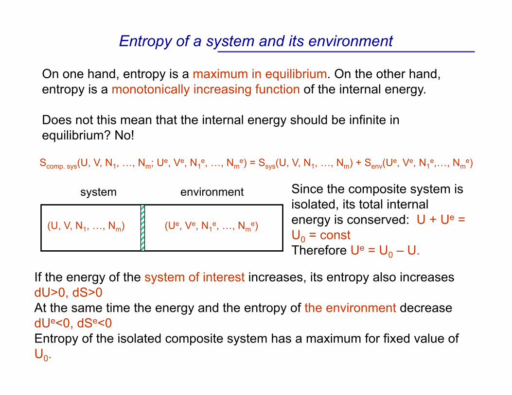
On one hand, entropy is a maximum in equilibrium. On the other hand, entropy is a monotonically increasing function of the internal energy.
Does not this mean that the internal energy should be infinite in equilibrium? No!
Scomp. sys(U, V, N1, …, Nm; Ue, Ve, N1e, …, Nm
e) = Ssys(U, V, N1, …, Nm) + Senv(Ue, Ve, N1e,…, Nm
e)
system environment
(U, V, N1, …, Nm) (Ue, Ve, N1e, …, Nm
e)
Since the composite system is isolated, its total internal energy is conserved: U + Ue = U0 = const Therefore Ue = U0 – U.
If the energy of the system of interest increases, its entropy also increases dU>0, dS>0 At the same time the energy and the entropy of the environment decrease dUe<0, dSe<0 Entropy of the isolated composite system has a maximum for fixed value of U0.
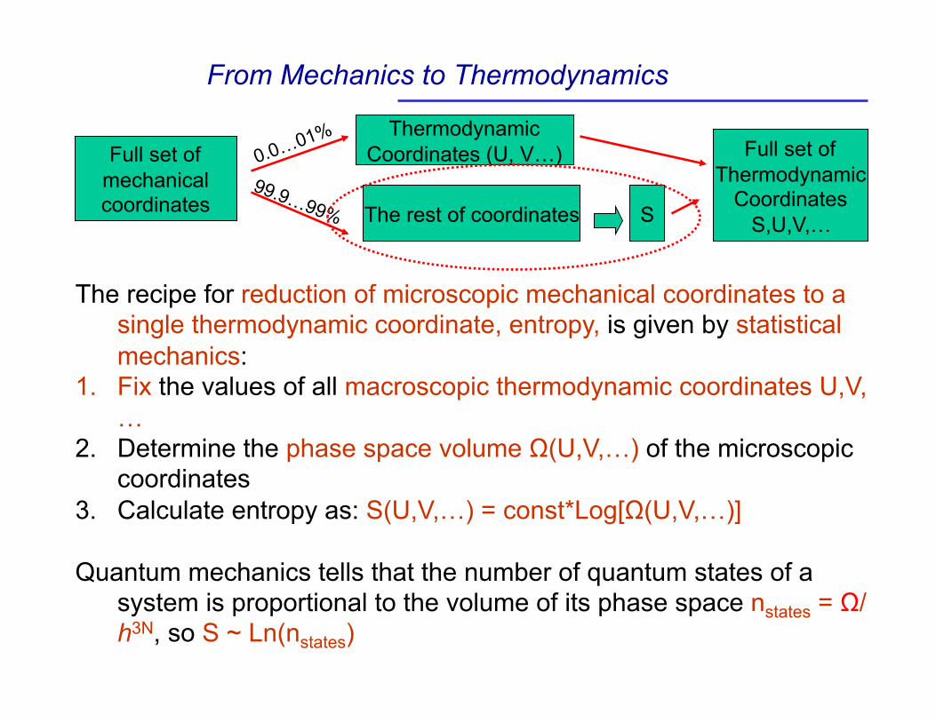
Full set of mechanical coordinates
Thermodynamic Coordinates (U, V…)
The rest of coordinates S
Full set of Thermodynamic
Coordinates S,U,V,…
From Mechanics to Thermodynamics
The recipe for reduction of microscopic mechanical coordinates to a single thermodynamic coordinate, entropy, is given by statistical mechanics:
1. Fix the values of all macroscopic thermodynamic coordinates U,V,…
2. Determine the phase space volume Ω(U,V,…) of the microscopic coordinates
3. Calculate entropy as: S(U,V,…) = const*Log[Ω(U,V,…)]
Quantum mechanics tells that the number of quantum states of a system is proportional to the volume of its phase space nstates = Ω/h3N, so S ~ Ln(nstates)
ln(Ω
syst
em)+
ln(Ω
envi
ronm
ent)
U…
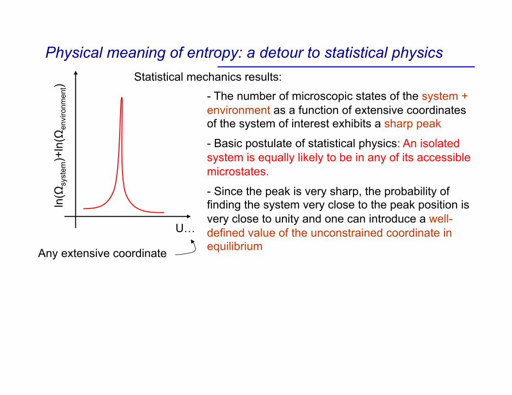
- The number of microscopic states of the system + environment as a function of extensive coordinates of the system of interest exhibits a sharp peak
- Basic postulate of statistical physics: An isolated system is equally likely to be in any of its accessible microstates.
- Since the peak is very sharp, the probability of finding the system very close to the peak position is very close to unity and one can introduce a well-defined value of the unconstrained coordinate in equilibrium
Physical meaning of entropy: a detour to statistical physics Statistical mechanics results:
Any extensive coordinate
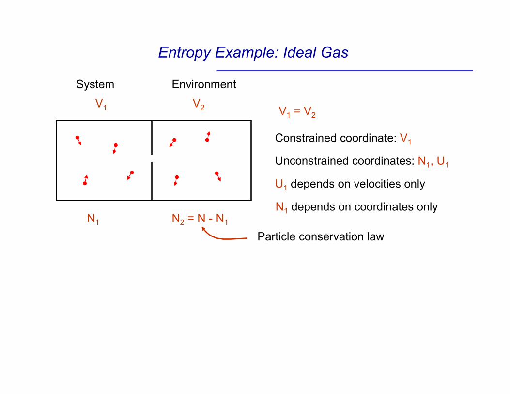
Entropy Example: Ideal Gas
V1 = V2
Constrained coordinate: V1
Unconstrained coordinates: N1, U1
U1 depends on velocities only
N1 depends on coordinates only
V1 V2
N1 N2 = N - N1 Particle conservation law
System Environment
Entropy Example: Ideal Gas
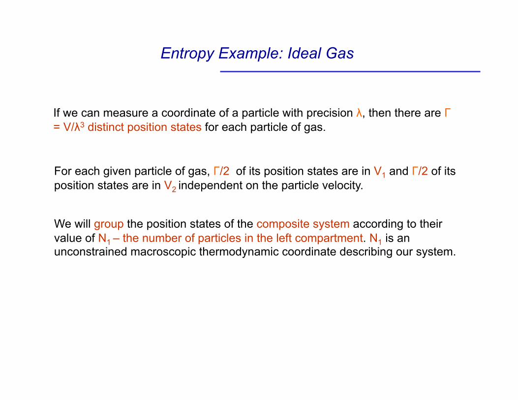
For each given particle of gas, Γ/2 of its position states are in V1 and Γ/2 of its position states are in V2 independent on the particle velocity.
We will group the position states of the composite system according to their value of N1 – the number of particles in the left compartment. N1 is an unconstrained macroscopic thermodynamic coordinate describing our system.
If we can measure a coordinate of a particle with precision λ, then there are Γ = V/λ3 distinct position states for each particle of gas.
Entropy Example: Ideal Gas
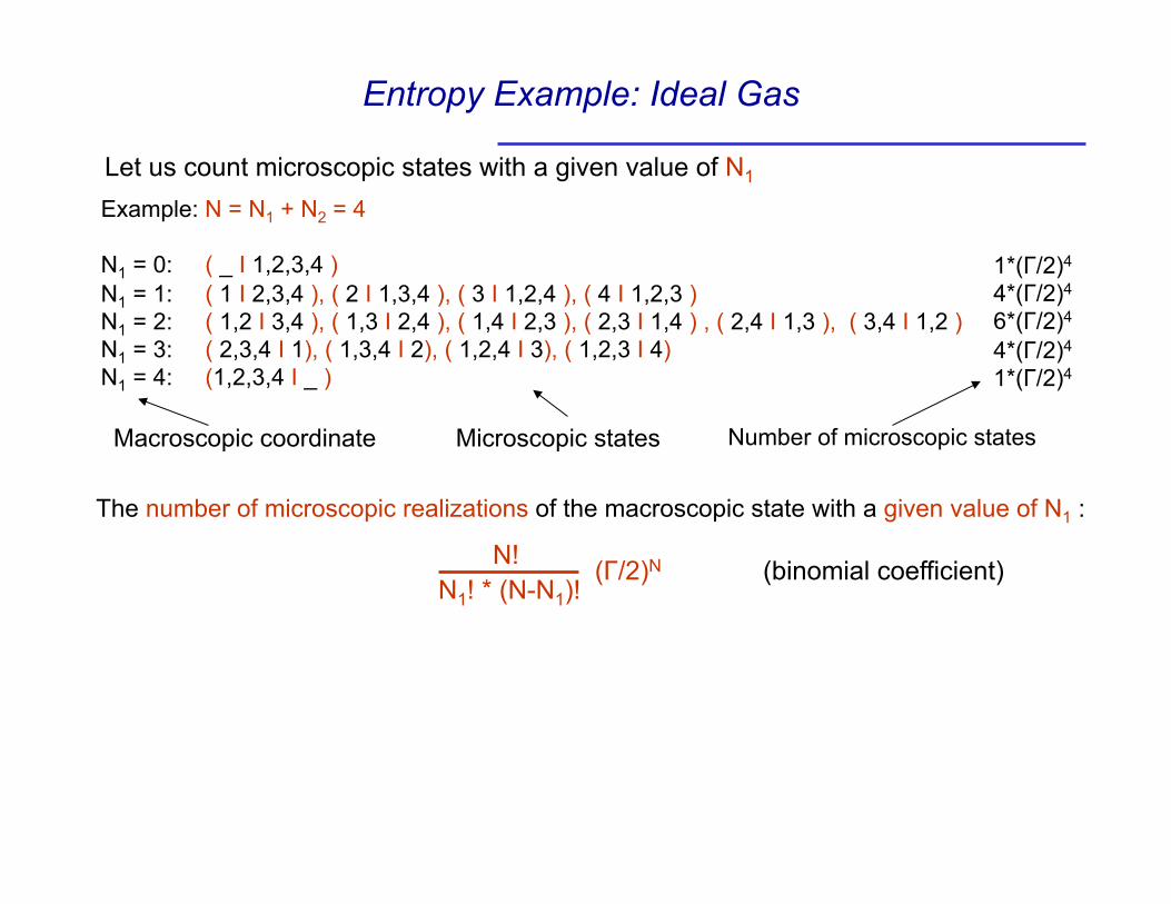
Example: N = N1 + N2 = 4
N1 = 0: ( _ I 1,2,3,4 ) N1 = 1: ( 1 I 2,3,4 ), ( 2 I 1,3,4 ), ( 3 I 1,2,4 ), ( 4 I 1,2,3 ) N1 = 2: ( 1,2 I 3,4 ), ( 1,3 I 2,4 ), ( 1,4 I 2,3 ), ( 2,3 I 1,4 ) , ( 2,4 I 1,3 ), ( 3,4 I 1,2 ) N1 = 3: ( 2,3,4 I 1), ( 1,3,4 I 2), ( 1,2,4 I 3), ( 1,2,3 I 4) N1 = 4: (1,2,3,4 I _ )
Macroscopic coordinate Microscopic states
The number of microscopic realizations of the macroscopic state with a given value of N1 :
1*(Γ/2)4
4*(Γ/2)4
6*(Γ/2)4
4*(Γ/2)4
1*(Γ/2)4
Number of microscopic states
N! N1! * (N-N1)!
(Γ/2)N (binomial coefficient)
Let us count microscopic states with a given value of N1
Entropy Example: Ideal Gas
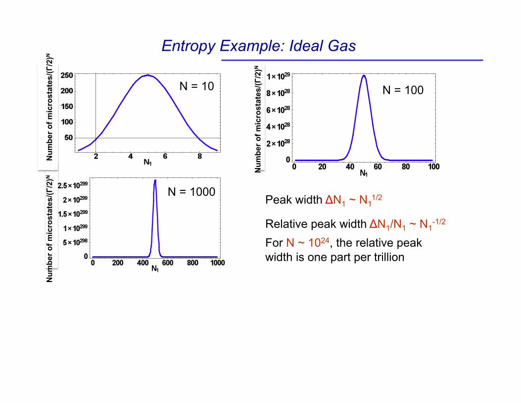
N = 10 N = 100
N = 1000 Peak width ΔN1 ~ N1
1/2
Relative peak width ΔN1/N1 ~ N1-1/2
For N ~ 1024, the relative peak width is one part per trillion
Num
ber o
f mic
rost
ates
/(Γ/2
)N
Num
ber o
f mic
rost
ates
/(Γ/2
)N
Num
ber o
f mic
rost
ates
/(Γ/2
)N
Entropy Example: Ideal Gas
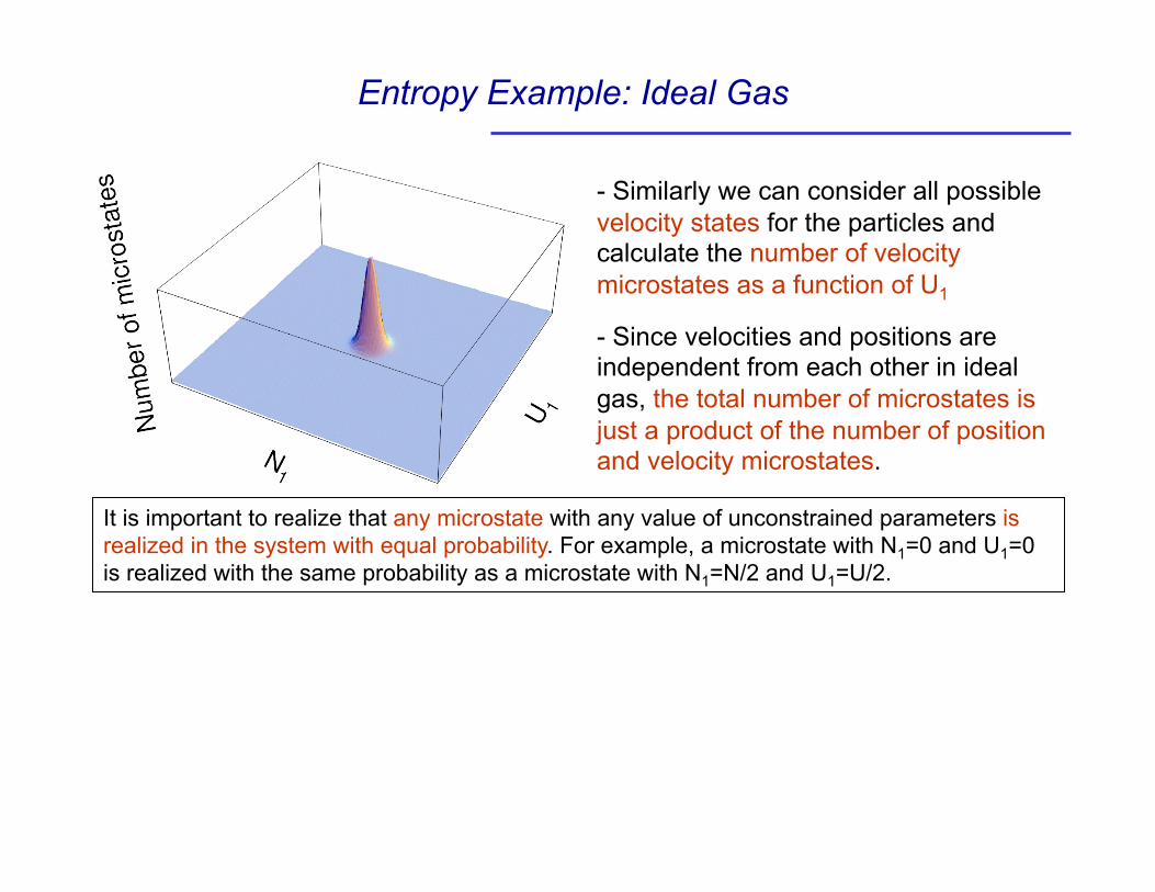
- Similarly we can consider all possible velocity states for the particles and calculate the number of velocity microstates as a function of U1
- Since velocities and positions are independent from each other in ideal gas, the total number of microstates is just a product of the number of position and velocity microstates.
It is important to realize that any microstate with any value of unconstrained parameters is realized in the system with equal probability. For example, a microstate with N1=0 and U1=0 is realized with the same probability as a microstate with N1=N/2 and U1=U/2.
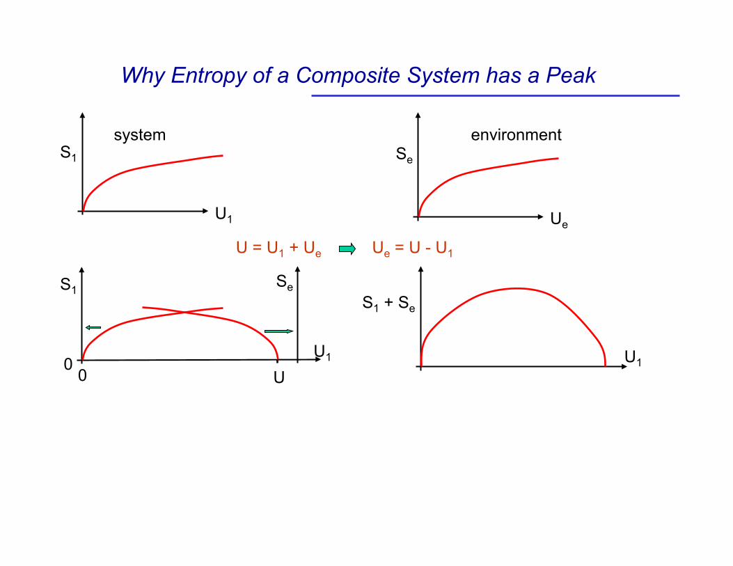
Why Entropy of a Composite System has a Peak
S1
U1
Se
Ue
U = U1 + Ue Ue = U - U1
S1 + Se
U1 U1
S1
U
Se
0 0
system environment
Irreversibility in Thermodynamics
A short description of thermodynamic processes: If a constraint between system and its environment is removed, entropy of the system + environment increases: dS = Sf - Si >0 (Postulate II). This is because by removing a constraint we have increased the volume of phase space that the microscopic coordinates of the system + environment can explore.
This means that a process Si Sf is allowed while the opposite process Sf Si is prohibited because it decreases the entropy of the composite system.
Thus irreversibility is inherent in thermodynamics. In mechanics, all processes are inherently reversible. In mechanics, it is sufficient to reverse all velocities to return to a state of the system in the past (essentially to go backwards in time).
Origins of Irreversibility
Origins of irreversibility: - Dynamic origins (tell you why reversing velocities does not get you to the initial state) - Kinematic origin (the most fundamental one)
Dynamic origins:
1. Isolated macroscopic systems is an abstraction. A typical system
with 1023 atoms has quantum energy spacing of ~ Joules.
For comparison, gravitational (weakest) interaction energy between two electrons at the opposite ends of observable universe is ~ 10-98 Joules. So a system as small as 100 particles cannot be truly isolated.
2. Even if we neglect interactions with the rest of the world, there are still interactions with fluctuations of the physical vacuum which are random in nature.
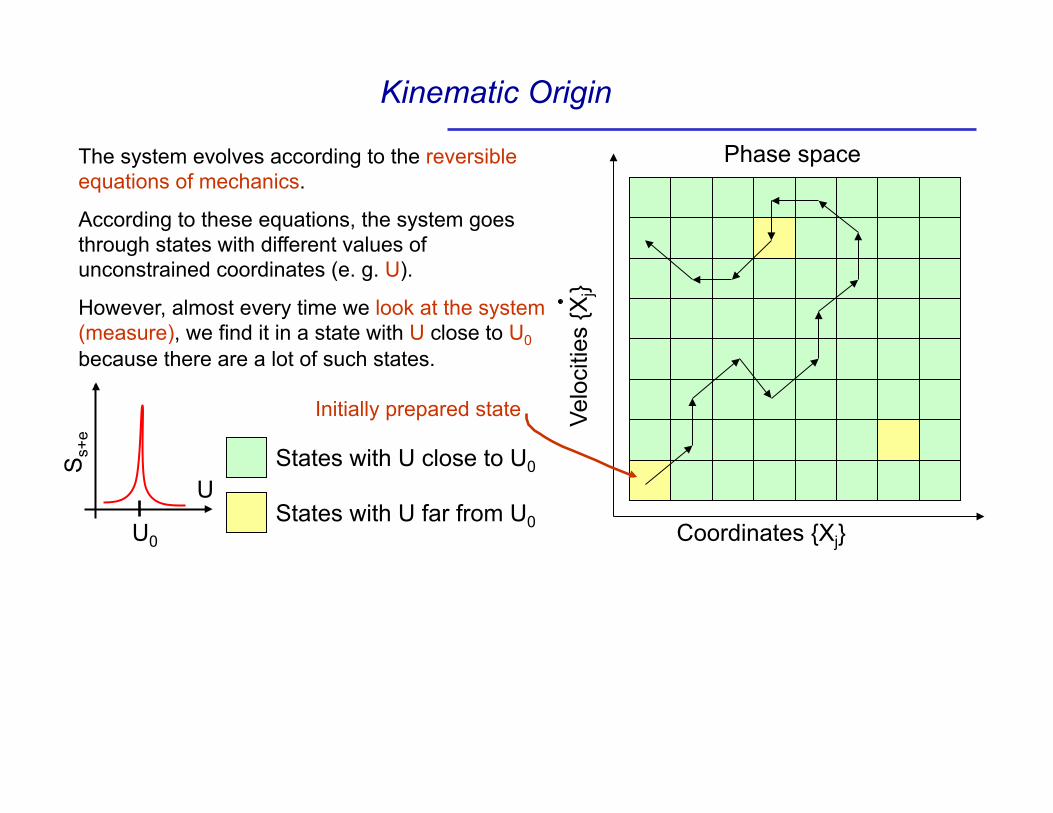
Kinematic Origin
Coordinates {Xj}
Velo
citie
s {X
j}
States with U close to U0
States with U far from U0
The system evolves according to the reversible equations of mechanics.
According to these equations, the system goes through states with different values of unconstrained coordinates (e. g. U).
However, almost every time we look at the system (measure), we find it in a state with U close to U0 because there are a lot of such states.
Ss+
e
U
U0
Initially prepared state
Phase space


![CHEMISTRY - Padasalai.Net-12th Study Materials are the postulates of valence bond theory (or) VB theory? [Mar 09] 17 5 & 10 Mark Question & Answers 7. In what way [ ]4- FeF 6 differ](https://img.pdfslide.tips/doc/110x75/5aadd2d87f8b9a25088b7351/chemistry-study-materials-are-the-postulates-of-valence-bond-theory-or-vb-theory.jpg)