Bank i Kredyt 48(1) , 2017, 1-44

The symmetry of demand and supply shocks in the European Monetary Union

Henryk Bąk*, Sebastian Maciejewski#

Submitted: 29 April 2016. Accepted: 3 November 2016.

AbstractIn this paper we apply the Blanchard and Quah (1988) SVAR methodology in order to estimate the size and frequency of demand and supply shocks for the EMU member countries in 1996−2014. Obtained SVAR estimates suggest that Eurozone’s largest economies – Germany, France and Italy – show the greatest similarity with the Eurozone under the criterion of shock correlation and amplitude. In turn, the majority of CEE countries, which are Eurozone’s latest joiners, exhibit relatively low correlations of demand and supply shocks with the euro area. The impact of the global financial crisis on the euro area’s economies is pronounced for all 16 analysed countries between 2008 Q4 and 2009 Q2. The comparison of shock correlations prior to and after the outbreak of the global financial crisis illustrates considerable changes in correlations of demand and supply shocks of individual countries with the euro area, where changes in the correlation of demand shocks are greater in magnitude, and positive changes in the correlation of demand shocks and negative changes in the correlation of supply shocks predominate.

Keywords: time series models, asymmetric shocks, the euro area

JEL: C32, E3, F36, F44

* Warsaw School of Economics, Collegium of World Economy; e-mail: hbak@sgh.waw.pl.# PGE Polska Grupa Energetyczna, Risk Department; e-mail: sebastian.michal.maciejewski@gmail.com.

H. Bąk, S. Maciejewski2

1 Introduction

By joining the monetary union countries abandon their national currencies and national monetary policies, thereby relinquishing an important instrument facilitating adjustment to shocks having asymmetric effect on the union’s member countries (asymmetric shocks). In the broad macroeconomic context, shocks can be defined as unexpected and significant changes that affect the economy. In a narrower sense, shocks refer to actual but unpredictable events that affect output and/or price levels, either positively or negatively. Asymmetric shocks are shocks that affect specific regions or countries in a different manner. According to the basic, traditional approach based on the AS-AD model, macroeconomic shocks are divided into demand- and supply-side shocks. Asymmetric shocks negatively affect business cycle synchronization within a monetary union and result in real exchange rate divergence between monetary union members. Adjustment to fluctuations in the real exchange rate constitutes cost for monetary union members.

The size, frequency and correlation of asymmetric shocks within the monetary union determine the need for real exchange rate adjustment between member countries. The size, frequency and correlation of shocks depend among others on the intensity of trade and economic integration, structural specialization within the union and relative competitiveness of individual member countries.

A smoothly functioning monetary union may be characterized by similar amplitude and high correlation of supply and demand shocks and/or high efficiency of smoothing mechanisms that can cushion the effects of asymmetric shocks. Adjustment to arising shocks can be effectuated by many mechanisms, among which, factor flexibility, counter-cyclical fiscal policy and financial markets are the most important.

In this paper we apply the identification scheme of Bayoumi and Eichengreen (1992), which is a modification of the Blanchard and Quah (1988) methodology, in order to analyse the size, frequency and correlation of shocks in the EMU in the most recent period of 1996−2014. The model identifies demand and supply shocks from the two-variable vector autoregression (VAR). Following the aggregate-demand-aggregate-supply (AS-AD) framework, serving as a theoretical basis for this method, macroeconomic shocks are decomposed into supply and demand shocks. Demand shocks are generated e.g. by shifts in investment demand, changes in domestic or foreign demand, consumer preference shifts, macroeconomic or fiscal policy changes, or changing perception of macroeconomic risk of a country. Supply shocks are unexpected events that affect output or disrupt the supply chain. They are caused by changes in technology, raw-materials price changes, mid- and long-term labour migration, or natural disasters. A detailed taxonomy of demand and supply shocks and sources of asymmetric shocks can be found in Borowski (2001, pp. 4−10). Within this framework, demand shocks have no long-run effect on output, while supply shocks affect the output level permanently.

The 1996−2014 period covers the time of the functioning of the Eurozone and its late formation phase. It is of our particular interest in this paper to inspect how correlations of shocks have changed after the outbreak of the global financial crisis in 2008, as compared with the 1996−2008 period. In this respect, our article updates the results presented in, i.a. Bayoumi and Eichengreen (1992), Firdmuc and Korhonen (2001), Frenkel and Nickel (2002) or Dumitru and Dumitru (2011), which were obtained for periods before the outbreak of the global financial crisis of 2008, or even before the formation of the euro area.

In this paper we find that the impact of the global financial crisis on the EA12 was particularly pronounced during 2008 Q4−2009 Q2. Our results point to the existence of large negative supply shocks

The symmetry of demand and supply shocks... 3

in all 16 Eurozone member countries. At the same time, demand shocks are found to be significantly smaller in size than supply shocks.

Our results for the 1996−2014 period show that the core countries of the Eurozone – Germany, France and Italy – are characterized by high correlation of supply shocks and medium correlation of demand shocks with the euro area. The three countries show the greatest similarity with the Eurozone under the criterion of supply and demand shock correlation whereas the CEE countries, which are the Eurozone’s latest joiners, generally exhibit relatively low correlations of demand and supply shocks, as compared to the EMU’s old members.

We also find that correlations of demand and supply shocks of individual countries with the euro area have changed considerably between 1996−2008 and 2010−2014. On average, changes in correlation of demand shocks have been greater in magnitude than changes in correlation of supply shocks. Also, positive changes in correlation of demand shocks and negative changes in the correlation of supply shocks have prevailed between 1996−2008 and 2010−2014. Interestingly, the EA12’s large economies (Germany, Italy and Spain), as well as the so-called ‘EMU-core’ countries (Belgium, the Netherlands) have become less suitable for the euro area under the correlation criterion of demand and supply shocks. By contrast, France, Finland, Austria, Slovakia and Latvia have become more suitable for the EMU under the same criterion.

The remaining part of this paper is organized as follows. Section 2 provides a brief literature review. Section 3 presents the method of decomposition of demand and supply shocks. Sections 4 and 5 focus on data and model specification issues. Sections 6 to 9 present estimation results. In these sections we assess the size and correlation of occurring shocks. Section 10 provides a brief discussion about whether shocks will increase or decrease in their size, frequency and correlation in the euro area in the near future. Finally, Section 11 concludes the analysis of this paper.

2 Literature review

The stream of economic literature focusing on the identification of demand and supply shocks by means of structural VAR models was started by Blanchard and Quah (1988), and later modified by Bayoumi and Eichengreen (1992).

In their paper, Bayoumi and Eichengreen (1992) assessed the advisability of the prospective currency union for the former 11 European Community (EC) members from the point of view of estimated shock size, frequency and correlation, and compared their results with the US – a smoothly functioning monetary union. The conclusions of their paper were that the EC was characterized by significantly greater shock asymmetry than the US, and that the frequency of supply shocks will decline and the correlation of shocks will increase in the EC along with market integration. Demand shocks, however, were expected to increase and become less correlated as specialization processes in the EC grew in strength.

The SVAR identification scheme proposed by Bayoumi and Eichengreen (1992) has become a standard model, often applied in economic research on the analysis of convergence and similarity of economic shocks in the euro area.

Applying Bayoumi and Eichengreen’s (1992) identification scheme, Firdmuc and Korhonen (2001) found that Italy, France, Spain and Germany had the highest correlations of supply and demand shocks

H. Bąk, S. Maciejewski4

with the euro area between 1991−2000. For these countries, correlations of supply shocks ranged from 0.52 to 0.69, while correlations of demand shocks varied between 0.16 and 0.57. For almost all countries the estimated individual correlations of demand shocks were considerably smaller than the respective correlations of supply shocks.

Frenkel and Nickel (2002) assessed the correlation of demand and supply shocks of individual euro area and CEE countries with euro area’s core countries for the period of 1995−2001. Their conclusion was that Belgium, Italy, France and Germany exhibited the highest correlations of supply shocks with the EMU – 0.99, 0.76, 0.74 and 0.62, respectively. By comparison, Belgium, Italy, France and Germany were characterized by the highest correlation of demand shocks – 0.94, 0.55, 0.35 and 0.31, respectively.

Finally, Dumitru and Dumitru (2011) evaluate correlations of individual euro area countries and NMS with the euro area. As for the individual euro area countries, they find that as a rule correlation of demand shocks was significantly lower than correlation of supply shocks. According to their estimates, Germany and Italy noted by far the highest correlations of demand and supply shocks with the Eurozone (roughly 0.9 for supply shocks and 0.65 for demand shocks each) during the 2003−2009 period. High correlation of supply shocks was also visible in the case of the Netherlands, Austria, Belgium, Slovenia and France, which ranged from 0.7 to 0.9. At the same time, estimated demand shocks in these countries were significantly more idiosyncratic, showing correlation coefficients ranging from -0.2 to 0.2.

While by means of the Bayoumi and Eichengreen (1992) method we identify macroeconomic shocks from the time series of GDP and inflation of each country and then investigate correlations between shocks across diverse economies, other researchers such as Ballabriga, Sebastian and Valles (1999) attempted to measure the interdependence relationships between countries modelled as a system. Through a BVAR model encompassing 4 countries, consisting of 12 “country-specific” and 3 “rest-of- -the world” variables, Ballabriga, Sebastian and Valles (1999) investigated the responses to common and country-specific, as well as nominal and real shocks in the group of countries consisting of Germany, France, UK and Spain. They differentiated between nominal and real sources of economic fluctuations as well as between the short- and long-term effects of shocks. Their results suggested that short-run idiosyncratic sources of fluctuations were the most prominent, implying that monetary unification in Europe is expected to be a costly venture.

In order to identify country-specific and regional shocks, Del Negro and Otrok (2008) develop a dynamic factor model with time-varying factor loadings and stochastic volatility to innovations in common factors and idiosyncratic components. Their model extracts information on the evolution of international business cycles from a large data set of several countries and decomposes fluctuations of countries’ GDP into country-specific shocks, region-specific shocks and fluctuations attributed to the international business cycle. The model results provide information on the sensitivity of countries to factors, on the volatility of business cycles and on business cycle synchronization among the selected countries. The authors find no evidence that business cycles changed in the euro area countries during 1970−2005.

Giannone, Lenza and Reichlin (2009) analyse the business cycle characteristics of the euro area countries between 1973 and 2006 by estimating a 12-variable VAR consisting of 12 GDP time series of the euro area countries. The model is first estimated on the time-period prior to the formation of the Eurozone, and then it is used to predict the expected path of a member country’s GDP in the EMU period, given the GDP of the euro area. The difference between the prediction of the model and

The symmetry of demand and supply shocks... 5

the actual path of GDP is used to infer whether intra-euro area relations have changed since the start of the EMU. Giannone, Lenza and Reichlin (2009) find that monetary unification has not affected business cycle characteristics and correlations of business cycles between the EMU countries.

Last but not least, some of the most recent studies, including Konopczak and Marczewski (2011), Skrzypczyński (2008) and Pietrzak (2014) investigate the similarity of business cycles and correlation of shocks with a particular focus on CEE countries – both EMU and non-EMU members.

The analysis focusing on the Polish economy and its performance after the outbreak of the global financial crisis, including an application of the Bayoumi and Eichengreen’s (1992) identification scheme and its extensions, can be found in Konopczak and Marczewski (2011). First, the authors extend the two-variable SVAR model by the real exchange rate, in order to differentiate between nominal and real demand shocks. Second, they propose another extension to a two-country framework, with GDP and CPI time series, where domestic and EMU variables enter the same model in order to differentiate between internal and external shocks affecting the economy. Konopczak and Marczewski (2011) conclude that the response of the Polish economy to the crisis of 2008/2009 was different from other CEE countries due to the structural characteristics of the Polish economy.

Finally, Pietrzak (2014) and Skrzypczyński (2008) investigate the degree of synchronization of business cycles between CEE states and the euro area by means of the cross-spectral method and analyse the correlation of cyclical components obtained from the Christiano-Fitzgerald band pass filter. Skrzypczyński (2008) finds that cyclical components of the real GDP of the CEE states are on average considerably less correlated with the euro area than the cyclical components of the core EMU members. Pietrzak (2014) concludes that the correlation of cyclical components of the CEE states with the Eurozone has increased in the vast majority of CEE countries after the outbreak of the global financial crisis.

3 The method of decomposition of demand and supply shocks

The bivariate SVAR model aimed at identifying disturbances that have a permanent effect on output (supply shocks) and temporary effect on output (demand shocks) was proposed by Blanchard and Quah (1988). This approach was later modified by Bayoumi and Eichengreen (1992), who applied the method to assess EU countries’ suitability for the prospective euro area. The model has become a standard model in the economic literature due to its relatively low degree of complexity and specification parsimony.

Bayoumi and Eichengreen (1992) proposed a decomposition method of shocks from the two- -variable VAR model to identify demand and supply shocks. This method departed from the AS-AD framework (see Figure 1).

In the left hand-side graph of Figure 1, the adjustment process to the demand shock is presented. In the right hand-side graph of Figure 1, the adjustment process to the supply shock is depicted. The starting point for analyses of output and price level responses to occurring demand and supply shocks is represented by the equilibrium point E1, with price level P1 and output level Y1, determined by the intersection of the AD (aggregate demand) and SARS (short-run aggregate supply) curves.

In the case of a positive demand shock – denoted by the shift of the AD curve to AD’ – both the price level and the output level increase in the short-run from the equilibrium level E1 to the

H. Bąk, S. Maciejewski6

equilibrium level E2. The E2 equilibrium level is characterized by the price level P2 and the output level Y2. In the long-run, it is only the price level that has increased in comparison to the level prior to the occurrence of the shock. The long-run equilibrium is denoted by point E3, with price level P3 and output level Y3 set by the intersection of the AD and LARS (long-run aggregate supply) curves. As a result of the appearance of the shock, the equilibrium price level has risen from P1 to P3. The output level, however, returns in the long-run to the level prior to the demand shock (Y3 is equal to Y1).

In the case of a positive supply shock – denoted by the shift of the SRAS curve to SRAS’ – the price level decreases from P1 to P2 and the output level increases from Y1 to Y2 in the short-run. The short-run equilibrium point E2 is set by the intersection of the AD and SRAS’ curves. In the long- -run, the price level further declines from P2 to P3, and the output level further grows from Y2 to Y3. As a result of the positive supply shock, the long-run supply curve shifts from LRAS to LRAS’. The long--run equilibrium level is denoted by point E3, characterized by the price level P3 and output level Y3, set by the intersection of the AD and LRAS’ curves. The state in which full adjustment to the positive supply shock has taken place in the long-run is characterized by lower price level P3 and greater output level Y3, as compared with the state prior to the occurrence of the shock (P1 and Y1); see Bayoumi and Eichengreen (1992, pp. 12−14).

In the Bayoumi and Eichengreen (1992) framework, the true model of demand and supply shocks is represented by the (two-variable) vector moving average VMA model of infinite order

==+++=

022110

kktktttt AAAAX

= =t

t ,tPYX

t

tt

2

1

=22,21,

12,11,

kk

kkk aa

aaA

tY

tP

t1 t2

( )INt ,0~

ijka ,

ijka , tj , ktiX +,

ktiijk Xa ,, = +

ktY +

=

=

+

=

+ ====0

11,,10 ,1

,111 0lim

kk

t

kt

nk t

kt aYX

tMtMtt uXBXBX +++= 11

( ) ( )( ) ====0

111

k=0kktkktkttMt CDuDuLBIuLBLBIX

( )INt ,0~ kk ACD =

=

tt Cu =

tt uCC 1:

( ) CLBLBIXM

lt

t 11==

=

=

..

.0

CC '

( )INt ,0~

ε ε ε

Δ

Δ

Δ

Δ

Δ

εε

ε

ε

εε

φ

ε

ε ε

ε

ε

ε

ε

ε

ε

Φ

Φ

Ω

tj ,ε

ε

ε∞

Σ

Σ Σ

ΣΣ

∞ ∞

∞

=0lΣ∞

∞

;

(1)

where:

==+++=

022110

kktktttt AAAAX

= =t

t ,tPYX

t

tt

2

1

=22,21,

12,11,

kk

kkk aa

aaA

tY

tP

t1 t2

( )INt ,0~

ijka ,

ijka , tj , ktiX +,

ktiijk Xa ,, = +

ktY +

=

=

+

=

+ ====0

11,,10 ,1

,111 0lim

kk

t

kt

nk t

kt aYX

tMtMtt uXBXBX +++= 11

( ) ( )( ) ====0

111

k=0kktkktkttMt CDuDuLBIuLBLBIX

( )INt ,0~ kk ACD =

=

tt Cu =

tt uCC 1:

( ) CLBLBIXM

lt

t 11==

=

=

..

.0

CC '

( )INt ,0~

ε ε ε

Δ

Δ

Δ

Δ

Δ

εε

ε

ε

εε

φ

ε

ε ε

ε

ε

ε

ε

ε

ε

Φ

Φ

Ω

tj ,ε

ε

ε∞

Σ

Σ Σ

ΣΣ

∞ ∞

∞

=0lΣ∞

∞

;

are vectors of dimension 2×1,

==+++=

022110

kktktttt AAAAX

= =t

t ,tPYX

t

tt

2

1

=22,21,

12,11,

kk

kkk aa

aaA

tY

tP

t1 t2

( )INt ,0~

ijka ,

ijka , tj , ktiX +,

ktiijk Xa ,, = +

ktY +

=

=

+

=

+ ====0

11,,10 ,1

,111 0lim

kk

t

kt

nk t

kt aYX

tMtMtt uXBXBX +++= 11

( ) ( )( ) ====0

111

k=0kktkktkttMt CDuDuLBIuLBLBIX

( )INt ,0~ kk ACD =

=

tt Cu =

tt uCC 1:

( ) CLBLBIXM

lt

t 11==

=

=

..

.0

CC '

( )INt ,0~

ε ε ε

Δ

Δ

Δ

Δ

Δ

εε

ε

ε

εε

φ

ε

ε ε

ε

ε

ε

ε

ε

ε

Φ

Φ

Ω

tj ,ε

ε

ε∞

Σ

Σ Σ

ΣΣ

∞ ∞

∞

=0lΣ∞

∞

;

is the matrix of

dimension 2×2,

==+++=

022110

kktktttt AAAAX

= =t

t ,tPYX

t

tt

2

1

=22,21,

12,11,

kk

kkk aa

aaA

tY

tP

t1 t2

( )INt ,0~

ijka ,

ijka , tj , ktiX +,

ktiijk Xa ,, = +

ktY +

=

=

+

=

+ ====0

11,,10 ,1

,111 0lim

kk

t

kt

nk t

kt aYX

tMtMtt uXBXBX +++= 11

( ) ( )( ) ====0

111

k=0kktkktkttMt CDuDuLBIuLBLBIX

( )INt ,0~ kk ACD =

=

tt Cu =

tt uCC 1:

( ) CLBLBIXM

lt

t 11==

=

=

..

.0

CC '

( )INt ,0~

ε ε ε

Δ

Δ

Δ

Δ

Δ

εε

ε

ε

εε

φ

ε

ε ε

ε

ε

ε

ε

ε

ε

Φ

Φ

Ω

tj ,ε

ε

ε∞

Σ

Σ Σ

ΣΣ

∞ ∞

∞

=0lΣ∞

∞

;

denotes the change in the volume of output,

==+++=

022110

kktktttt AAAAX

= =t

t ,tPYX

t

tt

2

1

=22,21,

12,11,

kk

kkk aa

aaA

tY

tP

t1 t2

( )INt ,0~

ijka ,

ijka , tj , ktiX +,

ktiijk Xa ,, = +

ktY +

=

=

+

=

+ ====0

11,,10 ,1

,111 0lim

kk

t

kt

nk t

kt aYX

tMtMtt uXBXBX +++= 11

( ) ( )( ) ====0

111

k=0kktkktkttMt CDuDuLBIuLBLBIX

( )INt ,0~ kk ACD =

=

tt Cu =

tt uCC 1:

( ) CLBLBIXM

lt

t 11==

=

=

..

.0

CC '

( )INt ,0~

ε ε ε

Δ

Δ

Δ

Δ

Δ

εε

ε

ε

εε

φ

ε

ε ε

ε

ε

ε

ε

ε

ε

Φ

Φ

Ω

tj ,ε

ε

ε∞

Σ

Σ Σ

ΣΣ

∞ ∞

∞

=0lΣ∞

∞

;

is the change in price level,

==+++=

022110

kktktttt AAAAX

= =t

t ,tPYX

t

tt

2

1

=22,21,

12,11,

kk

kkk aa

aaA

tY

tP

t1 t2

( )INt ,0~

ijka ,

ijka , tj , ktiX +,

ktiijk Xa ,, = +

ktY +

=

=

+

=

+ ====0

11,,10 ,1

,111 0lim

kk

t

kt

nk t

kt aYX

tMtMtt uXBXBX +++= 11

( ) ( )( ) ====0

111

k=0kktkktkttMt CDuDuLBIuLBLBIX

( )INt ,0~ kk ACD =

=

tt Cu =

tt uCC 1:

( ) CLBLBIXM

lt

t 11==

=

=

..

.0

CC '

( )INt ,0~

ε ε ε

Δ

Δ

Δ

Δ

Δ

εε

ε

ε

εε

φ

ε

ε ε

ε

ε

ε

ε

ε

ε

Φ

Φ

Ω

tj ,ε

ε

ε∞

Σ

Σ Σ

ΣΣ

∞ ∞

∞

=0lΣ∞

∞

;

and

==+++=

022110

kktktttt AAAAX

= =t

t ,tPYX

t

tt

2

1

=22,21,

12,11,

kk

kkk aa

aaA

tY

tP

t1 t2

( )INt ,0~

ijka ,

ijka , tj , ktiX +,

ktiijk Xa ,, = +

ktY +

=

=

+

=

+ ====0

11,,10 ,1

,111 0lim

kk

t

kt

nk t

kt aYX

tMtMtt uXBXBX +++= 11

( ) ( )( ) ====0

111

k=0kktkktkttMt CDuDuLBIuLBLBIX

( )INt ,0~ kk ACD =

=

tt Cu =

tt uCC 1:

( ) CLBLBIXM

lt

t 11==

=

=

..

.0

CC '

( )INt ,0~

ε ε ε

Δ

Δ

Δ

Δ

Δ

εε

ε

ε

εε

φ

ε

ε ε

ε

ε

ε

ε

ε

ε

Φ

Φ

Ω

tj ,ε

ε

ε∞

Σ

Σ Σ

ΣΣ

∞ ∞

∞

=0lΣ∞

∞

;

are respectively demand and supply shocks.

Shocks are assumed to be orthogonal and independent, which is characterized by the condition are respectively demand and supply shocks. Shocks are assumed to be orthogonal and independent, which is characterized by the condition

==+++=

022110

kktktttt AAAAX

= =t

t ,tPYX

t

tt

2

1

=22,21,

12,11,

kk

kkk aa

aaA

tY

tP

t1 t2

( )INt ,0~

ijka ,

ijka , tj , ktiX +,

ktiijk Xa ,, = +

ktY +

=

=

+

=

+ ====0

11,,10 ,1

,111 0lim

kk

t

kt

nk t

kt aYX

tMtMtt uXBXBX +++= 11

( ) ( )( ) ====0

111

k=0kktkktkttMt CDuDuLBIuLBLBIX

( )INt ,0~ kk ACD =

=

tt Cu =

tt uCC 1:

( ) CLBLBIXM

lt

t 11==

=

=

..

.0

CC '

( )INt ,0~

ε ε ε

Δ

Δ

Δ

Δ

Δ

εε

ε

ε

εε

φ

ε

ε ε

ε

ε

ε

ε

ε

ε

Φ

Φ

Ω

tj ,ε

ε

ε∞

Σ

Σ Σ

ΣΣ

∞ ∞

∞

=0lΣ∞

∞

;

. I is the identity matrix.

==+++=

022110

kktktttt AAAAX

= =t

t ,tPYX

t

tt

2

1

=22,21,

12,11,

kk

kkk aa

aaA

tY

tP

t1 t2

( )INt ,0~

ijka ,

ijka , tj , ktiX +,

ktiijk Xa ,, = +

ktY +

=

=

+

=

+ ====0

11,,10 ,1

,111 0lim

kk

t

kt

nk t

kt aYX

tMtMtt uXBXBX +++= 11

( ) ( )( ) ====0

111

k=0kktkktkttMt CDuDuLBIuLBLBIX

( )INt ,0~ kk ACD =

=

tt Cu =

tt uCC 1:

( ) CLBLBIXM

lt

t 11==

=

=

..

.0

CC '

( )INt ,0~

ε ε ε

Δ

Δ

Δ

Δ

Δ

εε

ε

ε

εε

φ

ε

ε ε

ε

ε

ε

ε

ε

ε

Φ

Φ

Ω

tj ,ε

ε

ε∞

Σ

Σ Σ

ΣΣ

∞ ∞

∞

=0lΣ∞

∞

;

are elements of the Ak matrix of impulse responses, where i and j denote respective row and column numbers.

==+++=

022110

kktktttt AAAAX

= =t

t ,tPYX

t

tt

2

1

=22,21,

12,11,

kk

kkk aa

aaA

tY

tP

t1 t2

( )INt ,0~

ijka ,

ijka , tj , ktiX +,

ktiijk Xa ,, = +

ktY +

=

=

+

=

+ ====0

11,,10 ,1

,111 0lim

kk

t

kt

nk t

kt aYX

tMtMtt uXBXBX +++= 11

( ) ( )( ) ====0

111

k=0kktkktkttMt CDuDuLBIuLBLBIX

( )INt ,0~ kk ACD =

=

tt Cu =

tt uCC 1:

( ) CLBLBIXM

lt

t 11==

=

=

..

.0

CC '

( )INt ,0~

ε ε ε

Δ

Δ

Δ

Δ

Δ

εε

ε

ε

εε

φ

ε

ε ε

ε

ε

ε

ε

ε

ε

Φ

Φ

Ω

tj ,ε

ε

ε∞

Σ

Σ Σ

ΣΣ

∞ ∞

∞

=0lΣ∞

∞

;

denotes the impact of

==+++=

022110

kktktttt AAAAX

= =t

t ,tPYX

t

tt

2

1

=22,21,

12,11,

kk

kkk aa

aaA

tY

tP

t1 t2

( )INt ,0~

ijka ,

ijka , tj , ktiX +,

ktiijk Xa ,, = +

ktY +

=

=

+

=

+ ====0

11,,10 ,1

,111 0lim

kk

t

kt

nk t

kt aYX

tMtMtt uXBXBX +++= 11

( ) ( )( ) ====0

111

k=0kktkktkttMt CDuDuLBIuLBLBIX

( )INt ,0~ kk ACD =

=

tt Cu =

tt uCC 1:

( ) CLBLBIXM

lt

t 11==

=

=

..

.0

CC '

( )INt ,0~

ε ε ε

Δ

Δ

Δ

Δ

Δ

εε

ε

ε

εε

φ

ε

ε ε

ε

ε

ε

ε

ε

ε

Φ

Φ

Ω

tj ,ε

ε

ε∞

Σ

Σ Σ

ΣΣ

∞ ∞

∞

=0lΣ∞

∞

;

shock on variable

==+++=

022110

kktktttt AAAAX

= =t

t ,tPYX

t

tt

2

1

=22,21,

12,11,

kk

kkk aa

aaA

tY

tP

t1 t2

( )INt ,0~

ijka ,

ijka , tj , ktiX +,

ktiijk Xa ,, = +

ktY +

=

=

+

=

+ ====0

11,,10 ,1

,111 0lim

kk

t

kt

nk t

kt aYX

tMtMtt uXBXBX +++= 11

( ) ( )( ) ====0

111

k=0kktkktkttMt CDuDuLBIuLBLBIX

( )INt ,0~ kk ACD =

=

tt Cu =

tt uCC 1:

( ) CLBLBIXM

lt

t 11==

=

=

..

.0

CC '

( )INt ,0~

ε ε ε

Δ

Δ

Δ

Δ

Δ

εε

ε

ε

εε

φ

ε

ε ε

ε

ε

ε

ε

ε

ε

Φ

Φ

Ω

tj ,ε

ε

ε∞

Σ

Σ Σ

ΣΣ

∞ ∞

∞

=0lΣ∞

∞

;

, i.e.

==+++=

022110

kktktttt AAAAX

= =t

t ,tPYX

t

tt

2

1

=22,21,

12,11,

kk

kkk aa

aaA

tY

tP

t1 t2

( )INt ,0~

ijka ,

ijka , tj , ktiX +,

ktiijk Xa ,, = +

ktY +

=

=

+

=

+ ====0

11,,10 ,1

,111 0lim

kk

t

kt

nk t

kt aYX

tMtMtt uXBXBX +++= 11

( ) ( )( ) ====0

111

k=0kktkktkttMt CDuDuLBIuLBLBIX

( )INt ,0~ kk ACD =

=

tt Cu =

tt uCC 1:

( ) CLBLBIXM

lt

t 11==

=

=

..

.0

CC '

( )INt ,0~

ε ε ε

Δ

Δ

Δ

Δ

Δ

εε

ε

ε

εε

φ

ε

ε ε

ε

ε

ε

ε

ε

ε

Φ

Φ

Ω

tj ,ε

ε

ε∞

Σ

Σ Σ

ΣΣ

∞ ∞

∞

=0lΣ∞

∞

;

.The constraint from the AS-AD model framework of no long-term effect of demand shock on

the level of output can be written as a sum of period effects of the demand shock

==+++=

022110

kktktttt AAAAX

= =t

t ,tPYX

t

tt

2

1

=22,21,

12,11,

kk

kkk aa

aaA

tY

tP

t1 t2

( )INt ,0~

ijka ,

ijka , tj , ktiX +,

ktiijk Xa ,, = +

ktY +

=

=

+

=

+ ====0

11,,10 ,1

,111 0lim

kk

t

kt

nk t

kt aYX

tMtMtt uXBXBX +++= 11

( ) ( )( ) ====0

111

k=0kktkktkttMt CDuDuLBIuLBLBIX

( )INt ,0~ kk ACD =

=

tt Cu =

tt uCC 1:

( ) CLBLBIXM

lt

t 11==

=

=

..

.0

CC '

( )INt ,0~

ε ε ε

Δ

Δ

Δ

Δ

Δ

εε

ε

ε

εε

φ

ε

ε ε

ε

ε

ε

ε

ε

ε

Φ

Φ

Ω

tj ,ε

ε

ε∞

Σ

Σ Σ

ΣΣ

∞ ∞

∞

=0lΣ∞

∞

;

on growth rates of output

==+++=

022110

kktktttt AAAAX

= =t

t ,tPYX

t

tt

2

1

=22,21,

12,11,

kk

kkk aa

aaA

tY

tP

t1 t2

( )INt ,0~

ijka ,

ijka , tj , ktiX +,

ktiijk Xa ,, = +

ktY +

=

=

+

=

+ ====0

11,,10 ,1

,111 0lim

kk

t

kt

nk t

kt aYX

tMtMtt uXBXBX +++= 11

( ) ( )( ) ====0

111

k=0kktkktkttMt CDuDuLBIuLBLBIX

( )INt ,0~ kk ACD =

=

tt Cu =

tt uCC 1:

( ) CLBLBIXM

lt

t 11==

=

=

..

.0

CC '

( )INt ,0~

ε ε ε

Δ

Δ

Δ

Δ

Δ

εε

ε

ε

εε

φ

ε

ε ε

ε

ε

ε

ε

ε

ε

Φ

Φ

Ω

tj ,ε

ε

ε∞

Σ

Σ Σ

ΣΣ

∞ ∞

∞

=0lΣ∞

∞

;

:

==+++=

022110

kktktttt AAAAX

= =t

t ,tPYX

t

tt

2

1

=22,21,

12,11,

kk

kkk aa

aaA

tY

tP

t1 t2

( )INt ,0~

ijka ,

ijka , tj , ktiX +,

ktiijk Xa ,, = +

ktY +

=

=

+

=

+ ====0

11,,10 ,1

,111 0lim

kk

t

kt

nk t

kt aYX

tMtMtt uXBXBX +++= 11

( ) ( )( ) ====0

111

k=0kktkktkttMt CDuDuLBIuLBLBIX

( )INt ,0~ kk ACD =

=

tt Cu =

tt uCC 1:

( ) CLBLBIXM

lt

t 11==

=

=

..

.0

CC '

( )INt ,0~

ε ε ε

Δ

Δ

Δ

Δ

Δ

εε

ε

ε

εε

φ

ε

ε ε

ε

ε

ε

ε

ε

ε

Φ

Φ

Ω

tj ,ε

ε

ε∞

Σ

Σ Σ

ΣΣ

∞ ∞

∞

=0lΣ∞

∞

;

(2)

The symmetry of demand and supply shocks... 7

The VMA representation of the data generating process (DGP) presented above is estimated through the VAR model, which is written as:

==+++=

022110

kktktttt AAAAX

= =t

t ,tPYX

t

tt

2

1

=22,21,

12,11,

kk

kkk aa

aaA

tY

tP

t1 t2

( )INt ,0~

ijka ,

ijka , tj , ktiX +,

ktiijk Xa ,, = +

ktY +

=

=

+

=

+ ====0

11,,10 ,1

,111 0lim

kk

t

kt

nk t

kt aYX

tMtMtt uXBXBX +++= 11

( ) ( )( ) ====0

111

k=0kktkktkttMt CDuDuLBIuLBLBIX

( )INt ,0~ kk ACD =

=

tt Cu =

tt uCC 1:

( ) CLBLBIXM

lt

t 11==

=

=

..

.0

CC '

( )INt ,0~

ε ε ε

Δ

Δ

Δ

Δ

Δ

εε

ε

ε

εε

φ

ε

ε ε

ε

ε

ε

ε

ε

ε

Φ

Φ

Ω

tj ,ε

ε

ε∞

Σ

Σ Σ

ΣΣ

∞ ∞

∞

=0lΣ∞

∞

;

(3)

B1…BM are matrices of estimated coefficients of dimension 2×2 and M being the selected lag order

of the VAR model. ut are residuals, which are by assumption ut ~ N(0, Ω), with being the variance- -covariance matrix.

From (3) it follows that:

==+++=

022110

kktktttt AAAAX

= =t

t ,tPYX

t

tt

2

1

=22,21,

12,11,

kk

kkk aa

aaA

tY

tP

t1 t2

( )INt ,0~

ijka ,

ijka , tj , ktiX +,

ktiijk Xa ,, = +

ktY +

=

=

+

=

+ ====0

11,,10 ,1

,111 0lim

kk

t

kt

nk t

kt aYX

tMtMtt uXBXBX +++= 11

( ) ( )( ) ====0

111

k=0kktkktkttMt CDuDuLBIuLBLBIX

( )INt ,0~ kk ACD =

=

tt Cu =

tt uCC 1:

( ) CLBLBIXM

lt

t 11==

=

=

..

.0

CC '

( )INt ,0~

ε ε ε

Δ

Δ

Δ

Δ

Δ

εε

ε

ε

εε

φ

ε

ε ε

ε

ε

ε

ε

ε

ε

Φ

Φ

Ω

tj ,ε

ε

ε∞

Σ

Σ Σ

ΣΣ

∞ ∞

∞

=0lΣ∞

∞

;

(4)

==+++=

022110

kktktttt AAAAX

= =t

t ,tPYX

t

tt

2

1

=22,21,

12,11,

kk

kkk aa

aaA

tY

tP

t1 t2

( )INt ,0~

ijka ,

ijka , tj , ktiX +,

ktiijk Xa ,, = +

ktY +

=

=

+

=

+ ====0

11,,10 ,1

,111 0lim

kk

t

kt

nk t

kt aYX

tMtMtt uXBXBX +++= 11

( ) ( )( ) ====0

111

k=0kktkktkttMt CDuDuLBIuLBLBIX

( )INt ,0~ kk ACD =

=

tt Cu =

tt uCC 1:

( ) CLBLBIXM

lt

t 11==

=

=

..

.0

CC '

( )INt ,0~

ε ε ε

Δ

Δ

Δ

Δ

Δ

εε

ε

ε

εε

φ

ε

ε ε

ε

ε

ε

ε

ε

ε

Φ

Φ

Ω

tj ,ε

ε

ε∞

Σ

Σ Σ

ΣΣ

∞ ∞

∞

=0lΣ∞

∞

;, and

==+++=

022110

kktktttt AAAAX

= =t

t ,tPYX

t

tt

2

1

=22,21,

12,11,

kk

kkk aa

aaA

tY

tP

t1 t2

( )INt ,0~

ijka ,

ijka , tj , ktiX +,

ktiijk Xa ,, = +

ktY +

=

=

+

=

+ ====0

11,,10 ,1

,111 0lim

kk

t

kt

nk t

kt aYX

tMtMtt uXBXBX +++= 11

( ) ( )( ) ====0

111

k=0kktkktkttMt CDuDuLBIuLBLBIX

( )INt ,0~ kk ACD =

=

tt Cu =

tt uCC 1:

( ) CLBLBIXM

lt

t 11==

=

=

..

.0

CC '

( )INt ,0~

ε ε ε

Δ

Δ

Δ

Δ

Δ

εε

ε

ε

εε

φ

ε

ε ε

ε

ε

ε

ε

ε

ε

Φ

Φ

Ω

tj ,ε

ε

ε∞

Σ

Σ Σ

ΣΣ

∞ ∞

∞

=0lΣ∞

∞

; is introduced as a transformation through which unobservable shocks εt are identified from VAR residuals through the estimated matrix

==+++=

022110

kktktttt AAAAX

= =t

t ,tPYX

t

tt

2

1

=22,21,

12,11,

kk

kkk aa

aaA

tY

tP

t1 t2

( )INt ,0~

ijka ,

ijka , tj , ktiX +,

ktiijk Xa ,, = +

ktY +

=

=

+

=

+ ====0

11,,10 ,1

,111 0lim

kk

t

kt

nk t

kt aYX

tMtMtt uXBXBX +++= 11

( ) ( )( ) ====0

111

k=0kktkktkttMt CDuDuLBIuLBLBIX

( )INt ,0~ kk ACD =

=

tt Cu =

tt uCC 1:

( ) CLBLBIXM

lt

t 11==

=

=

..

.0

CC '

( )INt ,0~

ε ε ε

Δ

Δ

Δ

Δ

Δ

εε

ε

ε

εε

φ

ε

ε ε

ε

ε

ε

ε

ε

ε

Φ

Φ

Ω

tj ,ε

ε

ε∞

Σ

Σ Σ

ΣΣ

∞ ∞

∞

=0lΣ∞

∞

;

.

The Φ matrix of accumulated long-run responses to structural shocks εt be defined as:

==+++=

022110

kktktttt AAAAX

= =t

t ,tPYX

t

tt

2

1

=22,21,

12,11,

kk

kkk aa

aaA

tY

tP

t1 t2

( )INt ,0~

ijka ,

ijka , tj , ktiX +,

ktiijk Xa ,, = +

ktY +

=

=

+

=

+ ====0

11,,10 ,1

,111 0lim

kk

t

kt

nk t

kt aYX

tMtMtt uXBXBX +++= 11

( ) ( )( ) ====0

111

k=0kktkktkttMt CDuDuLBIuLBLBIX

( )INt ,0~ kk ACD =

=

tt Cu =

tt uCC 1:

( ) CLBLBIXM

lt

t 11==

=

=

..

.0

CC '

( )INt ,0~

ε ε ε

Δ

Δ

Δ

Δ

Δ

εε

ε

ε

εε

φ

ε

ε ε

ε

ε

ε

ε

ε

ε

Φ

Φ

Ω

tj ,ε

ε

ε∞

Σ

Σ Σ

ΣΣ

∞ ∞

∞

=0lΣ∞

∞

;

(5)

Φ is the 2×2 matrix, with φij defining the long-run impact of shock in variable j on variable i. Given that ε1,t denotes the demand shock, the Φ matrix representing long-run impacts of shocks on dependent variables is restricted to the form:

==+++=

022110

kktktttt AAAAX

= =t

t ,tPYX

t

tt

2

1

=22,21,

12,11,

kk

kkk aa

aaA

tY

tP

t1 t2

( )INt ,0~

ijka ,

ijka , tj , ktiX +,

ktiijk Xa ,, = +

ktY +

=

=

+

=

+ ====0

11,,10 ,1

,111 0lim

kk

t

kt

nk t

kt aYX

tMtMtt uXBXBX +++= 11

( ) ( )( ) ====0

111

k=0kktkktkttMt CDuDuLBIuLBLBIX

( )INt ,0~ kk ACD =

=

tt Cu =

tt uCC 1:

( ) CLBLBIXM

lt

t 11==

=

=

..

.0

CC '

( )INt ,0~

ε ε ε

Δ

Δ

Δ

Δ

Δ

εε

ε

ε

εε

φ

ε

ε ε

ε

ε

ε

ε

ε

ε

Φ

Φ

Ω

tj ,ε

ε

ε∞

Σ

Σ Σ

ΣΣ

∞ ∞

∞

=0lΣ∞

∞

;

(6)

where the three remaining elements of Φ represented by dots need to be estimated.

In order to estimate the C matrix from the VAR, four restrictions need to be imposed. Three assumptions are described by the condition

==+++=

022110

kktktttt AAAAX

= =t

t ,tPYX

t

tt

2

1

=22,21,

12,11,

kk

kkk aa

aaA

tY

tP

t1 t2

( )INt ,0~

ijka ,

ijka , tj , ktiX +,

ktiijk Xa ,, = +

ktY +

=

=

+

=

+ ====0

11,,10 ,1

,111 0lim

kk

t

kt

nk t

kt aYX

tMtMtt uXBXBX +++= 11

( ) ( )( ) ====0

111

k=0kktkktkttMt CDuDuLBIuLBLBIX

( )INt ,0~ kk ACD =

=

tt Cu =

tt uCC 1:

( ) CLBLBIXM

lt

t 11==

=

=

..

.0

CC '

( )INt ,0~

ε ε ε

Δ

Δ

Δ

Δ

Δ

εε

ε

ε

εε

φ

ε

ε ε

ε

ε

ε

ε

ε

ε

Φ

Φ

Ω

tj ,ε

ε

ε∞

Σ

Σ Σ

ΣΣ

∞ ∞

∞

=0lΣ∞

∞

;

. The fourth restriction comes from the condition φl1 = 0, i.e. the restriction that demand shocks have only a temporary effect on output. Matrix C is estimated by the maximum likelihood, where

==+++=

022110

kktktttt AAAAX

= =t

t ,tPYX

t

tt

2

1

=22,21,

12,11,

kk

kkk aa

aaA

tY

tP

t1 t2

( )INt ,0~

ijka ,

ijka , tj , ktiX +,

ktiijk Xa ,, = +

ktY +

=

=

+

=

+ ====0

11,,10 ,1

,111 0lim

kk

t

kt

nk t

kt aYX

tMtMtt uXBXBX +++= 11

( ) ( )( ) ====0

111

k=0kktkktkttMt CDuDuLBIuLBLBIX

( )INt ,0~ kk ACD =

=

tt Cu =

tt uCC 1:

( ) CLBLBIXM

lt

t 11==

=

=

..

.0

CC '

( )INt ,0~

ε ε ε

Δ

Δ

Δ

Δ

Δ

εε

ε

ε

εε

φ

ε

ε ε

ε

ε

ε

ε

ε

ε

Φ

Φ

Ω

tj ,ε

ε

ε∞

Σ

Σ Σ

ΣΣ

∞ ∞

∞

=0lΣ∞

∞

;

. The likelihood function is evaluated in terms of unconstrained parameters.

Admittedly, the information on the size and frequency of demand and supply shocks provided by Bayoumi and Eichengreen’s (1992) identification scheme will imply very little about the exact source and character of economic shocks impacting individual countries. The scheme operates at a high level of macroeconomic generality for it requires a two-variable VAR, and distinguishes macroeconomic shocks impacting the economy according to one criterion only, i.e. demand shocks affecting output in the short-term, but not in the long-term, and supply shocks affecting the output level both in the short- and long-run, given independence of demand and supply shocks.

H. Bąk, S. Maciejewski8

4 Data

The data was collected from Eurostat’s quarterly national accounts database. The data consist of time series of real gross domestic product in EUR and the implicit GDP deflator. Following Bayoumi and Eichengreen (1992), the implicit GDP deflator has been chosen as an indicator of price level in the economy since it best reflects the price of total output in the economy, rather than the CPI index which only reflects the price level of consumption. Data concerning real gross domestic product in EUR and the implicit GDP deflator come as quarterly, not-seasonally adjusted time series.

Data cover the period of 1996−2014. The period after the outbreak of the financial crisis is of our special interest, since most of the literature on the topic of shock identification examines periods prior to the outbreak of the global financial crisis of 2008. The beginning of the estimation sample was selected in such a way as to ensure a sufficient number of observations to estimate the econometric model, and to include the maximum number of observations that are directly related to the functioning and the late phase of formation of the euro area. We take account of the fact that significant convergence in nominal exchange rates between countries that have formed the euro area in 2001 has been achieved by 1996.

The reference group for the demand and supply shock analysis are 12 countries of the Eurozone (EA12): Belgium, France, Germany, Ireland, Italy, Luxembourg, the Netherlands, Greece, Spain, Portugal, Austria and Finland. This is the reference group for our analysis due to the fact that the 12 countries formed the euro area already in 2001, and the convergence process preceding the adoption of the euro was started long before 2000 in these countries.

16 Eurozone member countries are subject to the analysis in this paper: Austria, Belgium, Estonia, Finland, France, Germany, Greece, Ireland, Italy, Latvia, Lithuania, the Netherlands, Portugal, Slovakia, Slovenia, and Spain. The smallest EMU countries – Cyprus, Luxembourg and Malta have not been included in the data set. Importantly, not all 16 of the countries in question have been members of the EMU since the beginning of 1999, which probably has a significant effect on the results of our analysis for these particular countries.

5 Analysis of selected variables. SVAR specification

We first examine the descriptive statistics of the time series that constitute input to the SVAR model. The selected time series are real GDP in EUR and implicit GDP deflator. Both time series start in 1996 Q3 and end in 2014 Q4.

In the first step, both time series were seasonally adjusted using the TRAMO/SEATS seasonal adjustment algorithm, in order to extract the seasonal component from the raw time series.

Then, both seasonally adjusted time series were tested for stationarity. The results of the augmented Dickey-Fuller (ADF) test are illustrated in Table 1. As for the real GDP, all but three of the examined time series are not stationary in the period of 1996−2014 at the 10% level according to the ADF test statistics. In turn, the real GDP series in first differences are stationary at the 10% probability level for all countries except for Spain, Greece and Italy.

Similarly, all the GDP deflator time series are not stationary in the 1996−2014 period at the 10% level, except for the case of Spain. In turn, all the GDP deflator series in the first differences are

The symmetry of demand and supply shocks... 9

stationary except for the case of Spain, Germany, Lithuania and Portugal. On the basis of the results of unit root analysis depicted in Table 1, all real GDP and GDP deflator series were log-1-st-differenced in preparation for the subsequent VAR estimation.

Next, we present the means and standard deviations of the log-first-differenced seasonally adjusted real GDP and GDP deflator time series in Table 2. It can be derived from Table 2 that countries with relatively high real GDP quarterly growth rates were also characterized by relatively high mean GDP deflator quarterly growth rates during the 1996−2014 period. This group of countries includes Estonia, Lithuania, Latvia and Slovakia.

Also, as a general rule, higher mean growth rates coincided with greater standard deviations of growth rates for both real GDP and GDP deflator series. This pattern is visible, among others, in the case of Estonia, Lithuania, Latvia, Slovenia and Slovakia, i.e. in the case of CEE countries – relatively small economies that joined the Eurozone between 2007 and 2015. In contrast, the largest euro area economies – Germany, France and Italy – are characterized by relatively low mean and standard deviations of real GDP and GDP deflator growth rates.

The correlation coefficients of real GDP and GDP deflator growth rates with the EA12 are reported in Table 3. Correlation coefficients of real GDP growth rates with the EA12 are presented in column 2, and correlation coefficients of GDP deflator growth rates with the EA12 are displayed in column 3 of Table 3.

The interesting observation derived from Table 3 is that the majority of EMU members who formed the euro area in 1999 have their real GDP growth rates strongly correlated with the EA12’s GDP growth rate throughout 1996−2014. The relatively low correlation coefficients obtained for Greece, Ireland and Portugal may be attributed to the impact of the global financial crisis on these economies. Relatively low correlation coefficients were also obtained for Latvia, Estonia and Slovakia – countries that were late joining the EMU, characterized by one of the highest real GDP growth rates in the time period under scrutiny.

The next modelling step consists of the optimal lag order selection for the VAR model that will be applied to all countries. Table 4 presents indications of the optimal lag order as indicated by the Akaike (AIC), Schwarz (SC) and Hannan-Quinn (HQ) information criteria. The majority of VAR lag order indications reported in Table 4 point to the selection of the VAR(1) or VAR(2) models.

Since our intention is to apply the same lag order to all VAR models to ensure the same model structure that has been applied to each country, we perform residual tests for the two candidate VAR models. More specifically, we perform residual tests for each individual country using the VAR(1) and VAR(2) models, in order to test for autocorrelation (LM test), normality (Jarque-Bera test) and heteroscedasticity (White test) of residuals.

The results for model VAR(1) are presented in Table 5. The probability levels associated with the three tests for VAR(1) model are reported for each country. In the majority of cases, the null hypotheses for the LM and JB test cannot be rejected at the 10% level. Furthermore, the results of the White test show that residuals may be heteroskedastic in 6 out of 17 VAR(1) specifications. The same tests have been re-done for the VAR(2) specification, although not reported in the paper. Overall, the three residual test results favour the VAR(1) model selection. As a result of the preceding analysis, the VAR model with lag order 1 was estimated for all the countries in order to assure the symmetry of model specification.

All models were estimated on the entire sample commencing in 1996 Q3 and ending in 2014 Q4. First, the choice of this estimation sample is primarily due to data availability – Eurostat’s quarterly

H. Bąk, S. Maciejewski10

real GDP and GDP deflator data for the majority of euro area countries is available from 1995 to 1997 onwards. Second, the start of global financial crisis, which had a considerable effect on GDP of all the examined countries in 2009 raises questions of whether and how to account for this unusual effect in VAR estimation.

On the one hand, the division of the entire 1996−2014 sample into 1996−2008 and 2009−2014 sub--samples and the estimation of VAR models on these separate samples is restricted due to the limited number of observations in the 2009−2014 period. On the other hand, treating the four observations from 2009 as outliers may lead to the state where important observations are not properly accounted for in the estimation. As a result, the approach we decided to follow is that one single VAR model is estimated for each country for the entire time period of 1996 Q3–2014 Q4.

6 Impulse response function and variance decomposition analysis

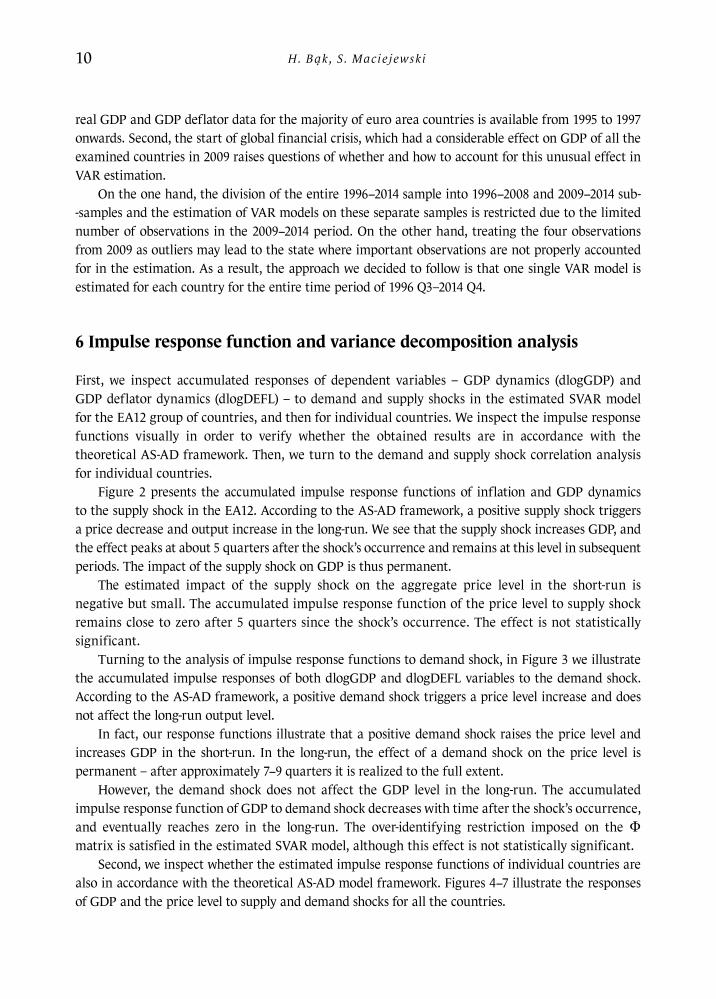
First, we inspect accumulated responses of dependent variables – GDP dynamics (dlogGDP) and GDP deflator dynamics (dlogDEFL) – to demand and supply shocks in the estimated SVAR model for the EA12 group of countries, and then for individual countries. We inspect the impulse response functions visually in order to verify whether the obtained results are in accordance with the theoretical AS-AD framework. Then, we turn to the demand and supply shock correlation analysis for individual countries.

Figure 2 presents the accumulated impulse response functions of inflation and GDP dynamics to the supply shock in the EA12. According to the AS-AD framework, a positive supply shock triggers a price decrease and output increase in the long-run. We see that the supply shock increases GDP, and the effect peaks at about 5 quarters after the shock’s occurrence and remains at this level in subsequent periods. The impact of the supply shock on GDP is thus permanent.

The estimated impact of the supply shock on the aggregate price level in the short-run is negative but small. The accumulated impulse response function of the price level to supply shock remains close to zero after 5 quarters since the shock’s occurrence. The effect is not statistically significant.

Turning to the analysis of impulse response functions to demand shock, in Figure 3 we illustrate the accumulated impulse responses of both dlogGDP and dlogDEFL variables to the demand shock. According to the AS-AD framework, a positive demand shock triggers a price level increase and does not affect the long-run output level.

In fact, our response functions illustrate that a positive demand shock raises the price level and increases GDP in the short-run. In the long-run, the effect of a demand shock on the price level is permanent – after approximately 7−9 quarters it is realized to the full extent.

However, the demand shock does not affect the GDP level in the long-run. The accumulated impulse response function of GDP to demand shock decreases with time after the shock’s occurrence, and eventually reaches zero in the long-run. The over-identifying restriction imposed on the Φ matrix is satisfied in the estimated SVAR model, although this effect is not statistically significant.

Second, we inspect whether the estimated impulse response functions of individual countries are also in accordance with the theoretical AS-AD model framework. Figures 4−7 illustrate the responses of GDP and the price level to supply and demand shocks for all the countries.

The symmetry of demand and supply shocks... 11

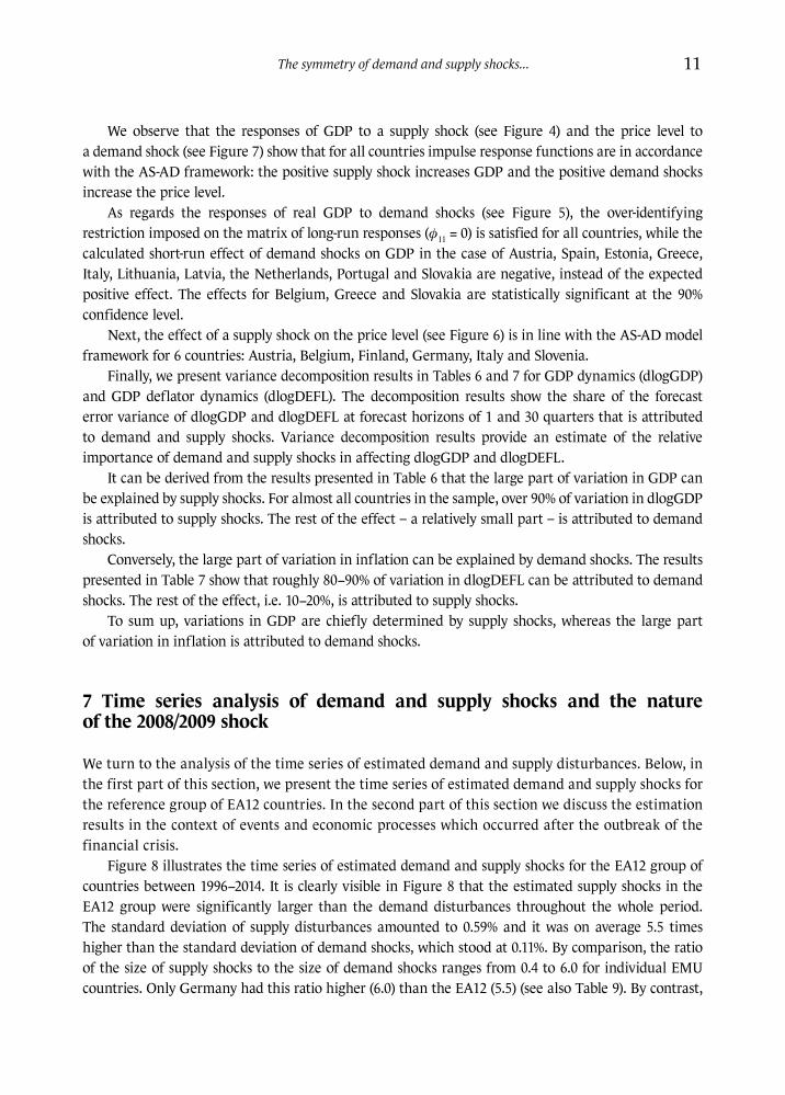
We observe that the responses of GDP to a supply shock (see Figure 4) and the price level to a demand shock (see Figure 7) show that for all countries impulse response functions are in accordance with the AS-AD framework: the positive supply shock increases GDP and the positive demand shocks increase the price level.

As regards the responses of real GDP to demand shocks (see Figure 5), the over-identifying restriction imposed on the matrix of long-run responses (φ11 = 0) is satisfied for all countries, while the calculated short-run effect of demand shocks on GDP in the case of Austria, Spain, Estonia, Greece, Italy, Lithuania, Latvia, the Netherlands, Portugal and Slovakia are negative, instead of the expected positive effect. The effects for Belgium, Greece and Slovakia are statistically significant at the 90% confidence level.

Next, the effect of a supply shock on the price level (see Figure 6) is in line with the AS-AD model framework for 6 countries: Austria, Belgium, Finland, Germany, Italy and Slovenia.

Finally, we present variance decomposition results in Tables 6 and 7 for GDP dynamics (dlogGDP) and GDP deflator dynamics (dlogDEFL). The decomposition results show the share of the forecast error variance of dlogGDP and dlogDEFL at forecast horizons of 1 and 30 quarters that is attributed to demand and supply shocks. Variance decomposition results provide an estimate of the relative importance of demand and supply shocks in affecting dlogGDP and dlogDEFL.

It can be derived from the results presented in Table 6 that the large part of variation in GDP can be explained by supply shocks. For almost all countries in the sample, over 90% of variation in dlogGDP is attributed to supply shocks. The rest of the effect – a relatively small part – is attributed to demand shocks.

Conversely, the large part of variation in inflation can be explained by demand shocks. The results presented in Table 7 show that roughly 80−90% of variation in dlogDEFL can be attributed to demand shocks. The rest of the effect, i.e. 10−20%, is attributed to supply shocks.

To sum up, variations in GDP are chiefly determined by supply shocks, whereas the large part of variation in inflation is attributed to demand shocks.

7 Time series analysis of demand and supply shocks and the nature of the 2008/2009 shock

We turn to the analysis of the time series of estimated demand and supply disturbances. Below, in the first part of this section, we present the time series of estimated demand and supply shocks for the reference group of EA12 countries. In the second part of this section we discuss the estimation results in the context of events and economic processes which occurred after the outbreak of the financial crisis.

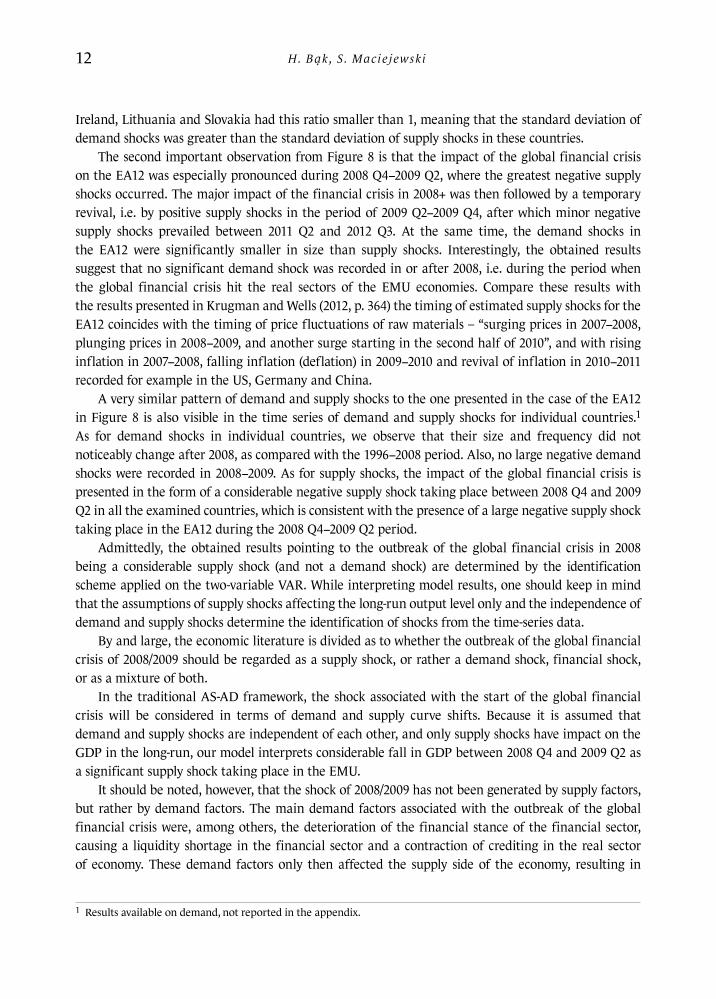
Figure 8 illustrates the time series of estimated demand and supply shocks for the EA12 group of countries between 1996−2014. It is clearly visible in Figure 8 that the estimated supply shocks in the EA12 group were significantly larger than the demand disturbances throughout the whole period. The standard deviation of supply disturbances amounted to 0.59% and it was on average 5.5 times higher than the standard deviation of demand shocks, which stood at 0.11%. By comparison, the ratio of the size of supply shocks to the size of demand shocks ranges from 0.4 to 6.0 for individual EMU countries. Only Germany had this ratio higher (6.0) than the EA12 (5.5) (see also Table 9). By contrast,

H. Bąk, S. Maciejewski12

Ireland, Lithuania and Slovakia had this ratio smaller than 1, meaning that the standard deviation of demand shocks was greater than the standard deviation of supply shocks in these countries.

The second important observation from Figure 8 is that the impact of the global financial crisis on the EA12 was especially pronounced during 2008 Q4−2009 Q2, where the greatest negative supply shocks occurred. The major impact of the financial crisis in 2008+ was then followed by a temporary revival, i.e. by positive supply shocks in the period of 2009 Q2−2009 Q4, after which minor negative supply shocks prevailed between 2011 Q2 and 2012 Q3. At the same time, the demand shocks in the EA12 were significantly smaller in size than supply shocks. Interestingly, the obtained results suggest that no significant demand shock was recorded in or after 2008, i.e. during the period when the global financial crisis hit the real sectors of the EMU economies. Compare these results with the results presented in Krugman and Wells (2012, p. 364) the timing of estimated supply shocks for the EA12 coincides with the timing of price fluctuations of raw materials – “surging prices in 2007−2008, plunging prices in 2008−2009, and another surge starting in the second half of 2010”, and with rising inflation in 2007−2008, falling inflation (deflation) in 2009−2010 and revival of inflation in 2010−2011 recorded for example in the US, Germany and China.

A very similar pattern of demand and supply shocks to the one presented in the case of the EA12 in Figure 8 is also visible in the time series of demand and supply shocks for individual countries.1 As for demand shocks in individual countries, we observe that their size and frequency did not noticeably change after 2008, as compared with the 1996−2008 period. Also, no large negative demand shocks were recorded in 2008−2009. As for supply shocks, the impact of the global financial crisis is presented in the form of a considerable negative supply shock taking place between 2008 Q4 and 2009 Q2 in all the examined countries, which is consistent with the presence of a large negative supply shock taking place in the EA12 during the 2008 Q4−2009 Q2 period.

Admittedly, the obtained results pointing to the outbreak of the global financial crisis in 2008 being a considerable supply shock (and not a demand shock) are determined by the identification scheme applied on the two-variable VAR. While interpreting model results, one should keep in mind that the assumptions of supply shocks affecting the long-run output level only and the independence of demand and supply shocks determine the identification of shocks from the time-series data.

By and large, the economic literature is divided as to whether the outbreak of the global financial crisis of 2008/2009 should be regarded as a supply shock, or rather a demand shock, financial shock, or as a mixture of both.

In the traditional AS-AD framework, the shock associated with the start of the global financial crisis will be considered in terms of demand and supply curve shifts. Because it is assumed that demand and supply shocks are independent of each other, and only supply shocks have impact on the GDP in the long-run, our model interprets considerable fall in GDP between 2008 Q4 and 2009 Q2 as a significant supply shock taking place in the EMU.

It should be noted, however, that the shock of 2008/2009 has not been generated by supply factors, but rather by demand factors. The main demand factors associated with the outbreak of the global financial crisis were, among others, the deterioration of the financial stance of the financial sector, causing a liquidity shortage in the financial sector and a contraction of crediting in the real sector of economy. These demand factors only then affected the supply side of the economy, resulting in

1 Results available on demand, not reported in the appendix.

The symmetry of demand and supply shocks... 13

a series of supply and demand shocks occurring repeatedly one after another, and having a much more significant effect on GDP than on inflation. More specifically, it was through securitization that the US housing market crisis was transferred out of the US banking sector to foreign banks all over the world. Financial problems of a few banks translated into the liquidity crisis on the European interbank markets. The liquidity crisis in the banking sector of the euro area has made commercial banks reduce lending to both firms and households. This, in turn, resulted in an increase in the cost of credit in the economy, being a source of major supply shocks in the euro area. The reduction in lending by commercial banks brought about a contraction in economic activity in the corporate sector and curbed investment spending in the economy. This constituted another demand shock to the economy. Companies began reducing costs of running business, and opted to reduce employment. As a result, the unemployment rate went up and, consequently, domestic demand fell. The limited domestic and foreign demand was another negative shock for companies wishing to sell their products. Companies lowered their production because of falling demand and cut their production costs further, leading to a further increase in unemployment and reduction of the domestic and foreign demand. As a result, GDP contracted and the weak domestic demand, falling export market demand and growing unemployment hampered economic recovery. These mechanisms reinforced each other, resulting in a series of supply and demand shocks, occurring repeatedly in the euro area in the period of 2009−2013 (see Marciniak 2010, pp. 26−31).

Importantly, the strong decline in output was accompanied by rather small changes in inflation. The low variability of inflation together with abrupt changes in output cause the applied identification scheme of Bayoumi and Eichengreen (1992) to associate the shock of 2008/2009 with the supply side, rather than the demand side. The estimates of variance decomposition of endogenous variables in our model, presented in the previous section, are also indicative of this result.

Finally, another strand of economic literature, having its origin in the outbreak of the global financial crisis of 2007/2008, treats financial shocks as a distinct type of shock, having their origin in the financial sector (Fornari, Stracca 2013, pp. 3−4). The outbreak of the global financial crisis of 2008/2009 is an example of the most recent significant financial shock.

Admittedly, the identification of financial shocks is difficult due to poor data availability and a lack of uniform approach towards financial shock identification. For example, Fornari and Stracca (2013) attempt to identify financial shocks in a VAR panel of 21 advanced countries. They attempt to identify financial shocks as shocks having an impact on the relative share price of the financial sector to the share price from the composite stock market index. Moreover, the financial shock should affect private investment and the supply of credit to the private sector. Their final condition for financial shock identification assumes the direction of the short-term response of the interest rate to the shock. Fornari and Stracca (2013) find that financial shocks can indeed be separated from other types of shocks, however, it is not evident whether financial shocks should be treated as demand or supply shocks in terms of their impact on the economy.

8 Correlation of demand and supply shocks

We now turn to the analysis of the correlation of demand and supply shocks of individual countries with the EA12 group. 16 EMU member countries are subject to our analysis. The analysis is divided

H. Bąk, S. Maciejewski14

into 3 time periods: the entire sample of 1996−2014 and 2 sub-samples: 1996−2008 and 2010−2014. Due to the significant negative symmetric effect of the global financial crisis on euro area economies, the year 2009 has been excluded from the post-2008 correlation analysis. This is why the second sub- -sample starts with 2010 Q1, instead of 2009 Q1.

Turning to the analysis of the correlation of shocks with the EA12, we first inspect correlations of aggregate demand and supply shocks with the EA12 group during the entire 1996−2014 period, which are presented in Table 8.

As to the supply shocks, the highest correlation of supply shocks with the EA12 was obtained for Germany (0.83), France (0.81), Italy (0.80) and the Netherlands (0.67). Germany, France and Italy are the EMU’s 3 largest economies. Admittedly, the large size of these economies has significant weight in the EA12 aggregate, and this may partly translate into high coefficients of correlation with the EA12.

Conversely, the group of countries with the lowest correlation of supply shocks with the EA12 is made up of Ireland (0.15), Slovakia (0.21) and Latvia (0.25). The relatively low correlations of supply shocks of these three countries might be determined by the high mean GDP growth rates in these countries between 1996 and 2014 relative to the EA12 average. Also, Ireland’s economy was one of the economies most severely hit by the global financial crisis in Europe, which surely translates into low correlation of supply shocks with the EA12.

To turn to demand shocks, we observe that the correlations of demand shocks of individual countries with the EA12 are generally lower than the correlation of supply shocks during the 1996–2014 period. Specifically, the demand shocks of Germany (0.65), Italy (0.46), France (0.32) and Spain (0.29) were most strongly correlated with the EA12. These four countries are the EMU’s largest economies.

By comparison, the lowest correlation coefficients of demand shocks with the EA12 were recorded for Lithuania (-0.37), Slovakia (-0.03), Estonia (0.03), Latvia (0.04), Portugal (0.05) and Ireland (0.06). The first four economies are EMU late joiners from the CEE region. The last two economies were severely hit by the global financial crisis of 2008+. This is most likely reflected in these numbers.

The results for the 1996−2014 period reported in columns 2 and 3 in Table 8 are also presented in graphic form in Figure 9. Should the highest correlation of supply and demand shocks be the only criterion for the country’s suitability for the Eurozone (with preference given to the correlation of supply shocks due to their permanent effect on output), then, according to the results from the 1996−2014 period, the core of the EMU should at least include Germany, Italy and France. The remaining group of countries with relatively high correlation of supply and demand shocks consists of the Netherlands, Spain, Slovenia and Finland.

Countries that were likely to face the highest costs of belonging to the EMU during 1996−2014, according to the shock correlation criterion, disregarding the smoothing effect of various economic processes and risk sharing channels that may attenuate the occurrence of asymmetric shocks, are Slovakia, Latvia, Ireland and Lithuania. We note, however, that Slovakia, Latvia, and Lithuania were not Eurozone members until 2009, 2014 and 2015, respectively. Admittedly, the pursuit of independent monetary policies by these countries prior to their accession to the EMU may have also generated shocks which cannot be directly measured in this two-variable SVAR.

Altogether, the obtained correlation coefficients of supply and demand shocks of individual countries for the period of 1996−2014 are within the similar value range that was obtained, among others, in papers by Dumitru and Dumitru (2011), Firdmuc and Korhonen (2001) and Frenkel and Nickel (2002). Also, similarly to the above papers, our estimates of correlation coefficients of supply

The symmetry of demand and supply shocks... 15

shocks for individual countries are generally visibly higher than correlations of demand shocks. Finally, Germany, France, Italy and the Netherlands were assessed as the most suitable members of the EMU in the above 3 papers, due to their relatively high symmetry of supply and demand shocks. Our results show a similar picture of the euro area’s core in the 1996−2014 period, and are rather consistent with the general perception that these countries form the core of the EMU.

Now, we turn to decomposing the 1996−2014 period into two sub-periods in order to inspect how the global financial crisis of 2008+ affected the correlation patterns of demand and supply disturbances of individual countries with the EA12 group. The estimation results for 1996−2008 are presented in columns 4 and 5 of Table 8. A graphic representation of the results for 1996−2014 is provided in Figure 10.

As far as supply shocks are concerned, the highest correlation of supply shocks with the EA12 was observed for Germany (0.83), France (0.79), Italy (0.76) and the Netherlands (0.72). These results are similar to the results reported for the 1996−2014 period. Again, the lowest correlation of supply shocks with the EA12 was estimated for Slovakia (-0.19) and Lithuania (0.14).

As for demand shocks, the strongest correlation with EA12 demand shocks was observed for Germany (0.77), Italy (0.48), Spain (0.36) and Slovenia (0.31), while the weakest correlation was estimated for Lithuania (-0.38), Estonia (-0.12), Slovakia (0.10) and Latvia (-0.08).

Overall, Germany, France, Italy and the Netherlands formed the group of EMU countries with the highest supply and demand shock correlation with the EA12 group during 1996−2008. The core EMU group could be alternatively extended by Slovenia, Austria, Greece, Belgium or Spain.

Also, Lithuania and Slovakia were the countries with by far the lowest correlations of demand and supply shocks with the EA12. We again remark that both Slovakia and Lithuania were not EMU members until 2009 and 2015, and correlations of demand and supply disturbances may have been affected by the pursuit of individual monetary policies.

Finally, we analyse the correlations of demand and supply shocks during the 2010−2014 period. Results for this period are reported in columns 6 and 7 of Table 8, and in Figure 11.

As to supply shocks in 2010−2014, the highest correlation of supply disturbances with the EA12 was estimated for Germany (0.82), Italy (0.75), France (0.75), Finland (0.70) and Slovenia (0.67). By contrast, the lowest correlation of supply shocks with the EA12 was recorded in the case of Slovakia (0.04), Estonia (0.20), Ireland (0.20) and Portugal (0.24).

It is Finland (from 39 to 70), Lithuania (from 0.14 to 0.47), Slovakia (from -0.19 to 0.04) and Slovenia (from 54 to 67) that posted significant rises in correlation of supply shocks between 1996−2008 and 2010−2014. Correlations of supply shocks did not significantly change for Germany, Italy and France, while the Netherlands (from 0.72 to 0.16), Belgium (from 0.62 to 0.38), Greece (from 0.53 to 0.33), Estonia (from 0.38 to 0.20) and Ireland (from 0.33 to 0.21) recorded the largest falls in the correlation of supply shocks between the two periods.

As to demand shocks during 2010–2014, the strongest correlation with the EA12 was recorded for France (0.59), Greece (0.59), Finland (0.47), Slovakia (0.46) and Germany (0.43). The weakest correlation was found for Lithuania (-0.50), Portugal (-0.07) and Latvia (-0.09).

As for changes in correlations, it is Slovakia (from -0.10 to 0.46), Estonia (-0.12 to 0.25), France (from 0.22 to 0.59) and Finland (from 0.21 to 0.47) that recorded the greatest increases in correlation coefficients of demand shocks between 1996−2008 and 2010−2014. In turn, Germany (from 0.77 to 0.43), Italy (from 0.48 to 0.19) and Spain (from 0.36 to 0.22) recorded the largest declines in this respect.

H. Bąk, S. Maciejewski16

Interestingly, candidates to form the core of the EMU under the correlation of supply and demand shocks criterion are more difficult to point at in the 2010−2014 period as compared with 1996−2008. The likely core EMU member countries selected on the basis of correlation coefficients of demand and supply shocks for 2010−2014 are France, Germany, Finland, and possibly Italy, Slovenia and Austria. Conversely, the least suitable in terms of correlations of supply and demand shocks are Ireland, Portugal, Latvia and Lithuania.

At least four interesting patterns can be derived from the comparison of supply and demand shock correlations between 1996−2008 and 2010−2014.

First, half of the countries analysed in this paper had their correlation of demand shocks increase in 2010−2014 as compared with 1996−2008. On average, increases in correlation of demand shocks were significantly greater in magnitude than declines in correlation. For one thing, the correlation of demand shocks increased visibly between 1996−2008 and 2010−2014 in Slovakia, Estonia, France, Finland, Greece, Austria, Belgium and Latvia. For another thing, the group of countries that recorded falling correlation coefficients of demand shocks between the two periods is made up of Germany, Italy, Spain, Lithuania, the Netherlands, Portugal and Slovenia. Importantly, the core countries of the EA12 group, i.e. Germany, Italy, Spain and the Netherlands, have recorded considerable decreases in demand shock correlation in this period.

Second, we observe that declines in correlation of supply shocks have been on average visibly greater in magnitude than the increases in correlation. On the one hand, the correlation of supply shocks went up between 1996−2008 and 2010−2014 in Lithuania, Finland, Slovakia, Slovenia, Spain and Latvia. On the other hand, the correlation coefficient of supply shocks declined for the Netherlands, Belgium, Greece, Estonia, Ireland, Portugal, France, Germany and Italy.

Third, when analysing the changes of correlation coefficients of both demand and supply shocks between 1996−2008 and 2010−2014, it becomes apparent that the EA12’s largest economies – Germany, Italy and Spain – as well as the so-called ‘EMU-core’ countries – Belgium and the Netherlands – became less suitable for the euro area under the criterion of the demand and supply shock correlation criterion. These countries experienced a substantial decline in at least one of the two correlation coefficients between 1996−2008 and 2010−2014. On the contrary, France, Austria, Finland, Slovakia and Latvia clearly became more suitable members of the EMU, with both correlation coefficients increasing between 1996−2008 and 2010−2014.

Finally, under the correlation of supply and demand shocks criterion, which is indicative of the country’s suitability for the Eurozone, Germany, France and Italy form the core of the EMU in the two analysed sub-periods. The group of other countries which show a high degree of synchronization with the EA12 consists of Slovenia and Finland. Interestingly, it is characteristic for Italy and France that their supply shocks were highly correlated with the EA12, while their correlations of demand shocks varied substantially between the two sub-periods.

It is also worth mentioning that the correlation of both demand shocks and supply shocks was moderate and stable in the case of the Spanish and Austrian economies across 1996−2008 and 2010−2014. As to Ireland, Slovakia, Latvia and Lithuania, these countries exhibited the lowest degree of symmetry of their demand or supply shocks with the EA12. Admittedly, Slovakia, Latvia and Lithuania were not EMU members until 2009, 2014 and 2015, and the pursuit of individual monetary policies may have had an effect on the estimated correlations of shocks.

The symmetry of demand and supply shocks... 17

9 The size of demand and supply shocks

In this section we compare the average size of the countries’ demand and supply shocks with the EA12. The results from this analysis are presented in Table 9. We juxtapose the average sizes of shocks expressed in terms of standard deviations with respective correlation coefficients for individual countries.

Principally, the degree of shock correlation alone does not determine a country’s suitability for the monetary union. Apart from the degree of shock symmetry expressed in terms of correlation coefficients, it is the size of shocks between countries that is of equal importance. This is because the low symmetry of shocks does not directly imply high costs of participation in the monetary union unless the size of shocks is sufficiently large. The worst case scenario for the monetary union is the case where the correlation of shocks is low and the size of shocks is high. In such a case, the cost of participation in the monetary union will be the greatest.

By inspecting standard deviations of demand and supply shocks, we would like to gain information about the size of shocks each country experienced during the 1996−2014 period. The average size of supply and demand shocks is reported as standard deviation of estimated shocks during 1996−2014 in columns 2 and 3 of Table 9.

Primarily, the size of either demand or supply shocks in the examined group of countries seems to be neither visibly correlated with the size of GDP nor geographical proximity. The only straightforward characteristic of countries whose shocks are relatively large is their geographical affiliation with the CEE region. Admittedly, by joining the EMU, relatively small CEE countries expect their shocks to become more correlated with the Eurozone’s core countries and simultaneously reduce the size of shocks appearing in these countries.

Next, in Figures 12 and 13 we juxtapose the magnitude of disturbances with their correlation with the EA12.

In Figure 12 we depict standard deviations and correlations of supply shocks with the EA12 for individual countries during 1996−2014. We conclude that there is no clear relationship between the size and the correlation of supply shocks in the analysed sample of countries. For one thing, the group of countries with relatively low standard deviation of shocks consists of countries with both relatively high and low correlations of supply shocks. For another thing, countries with relatively high standard deviation of supply shocks are characterized by moderate or low levels of supply shock correlation.

In Figure 13 we present standard deviations of demand shocks and demand shock correlation with the EA12 for individual countries in 1996−2014. In the case of demand shocks, the relationship between the size and correlation of shocks is marked, i.e. the correlation of demand shocks increases as the average size of demand shocks declines.

Based on visual inspection of Figure 13, we distinguish the following subgroups of countries. The first subgroup consists of Germany only. Germany has by far the highest correlation of demand shocks with the EA12 and one of the lowest standard deviations of demand shocks and is the best-suited member of the euro area under the criterion of demand shock size and correlation. The second group of countries is characterized by relatively high or moderate degree of demand shock correlation and a relatively low size of these shocks. Countries belonging to this group are well-fitting participants of the EMU according to the correlation criterion. Last, Latvia, Lithuania and Slovakia have the lowest correlations of demand shocks and the largest sizes of demand shocks among the examined countries.

H. Bąk, S. Maciejewski18

Latvia, Slovakia and Lithuania seem to be the least congruent with the euro area according to the above criterion.

All in all, under the joint criterion of supply and demand shock correlation and the size of supply and demand shocks based on results from the 1996−2014 period, we conclude that Germany, France and Italy are the best-fitting countries in the EMU. Next, Spain, the Netherlands, Austria, Slovenia and Finland are among countries with a moderate degree of alignment to the EMU. Slovakia, Latvia, Estonia and Lithuania are the least congruent with the EMU under the criterion of shock correlation and size.

10 The size and symmetry of shocks in the near future

The correlation analysis of demand and supply shocks illustrates the current tendencies in the EMU; however, it does not address the question whether shocks will increase or decrease in their size, frequency and correlation in the near future. This question can be at least partly addressed through the analysis of two main effects at play in the monetary union – the endogeneity effect and structural divergence tendencies.

If the endogeneity effect is relatively strong and structural divergence tendencies are not dominant in the future, the EMU is likely to function smoothly in the long run and shocks are likely to be smaller, less frequent and asymmetric. According to the endogeneity theory of OCA developed by Frankel and Rose (1996), the formation of a monetary union should facilitate the convergence of business cycles among countries within the monetary union through trade integration. With the elimination of the exchange rate risk and transaction costs in the trade of goods and services, intra monetary union trade is expected to augment and this will lead to greater convergence of member economies within the monetary union.

The already realized effect of unification on trade is visible and amounts to roughly 5–10% over 1995–2005 according to Nitsch and Pisu (2008), 8–23% up to 2008 according to Rose (2008), and 15% up to 2006 according to Frankel (2010).

However, if structural divergence tendencies prevail, monetary union will become costlier and it will have to rely more on available smoothing mechanisms. Bayoumi and Eichengreen (1992), Krugman (1993) and Kalemli-Ozcan, Sørensen and Yosha (1999) suggested that the integration process in the course of or after monetary unification may well be accompanied by an increase in specialization. Low barriers to trade, low transportation costs and significant positive concentration externalities will rather induce countries to specialize in different industries and the rise in specialization will eventually lead to more asymmetric output fluctuations.

The discussion on the importance of both effects is particularly important in the context of the current and future functioning of the EMU. In the current economic context, it is not obvious whether convergence or divergence tendencies will be dominant in the mid- to long-term future.

The recent global financial crisis of 2008+ has visibly strengthened different divergence tendencies in the euro area, thereby creating significant economic strains between member countries. Divergence tendencies are visible in competitiveness (Molle 2015) and productivity levels (Fingleton, Garretsen, Martin 2015; Beck, Grodzicki 2014), as well as in economic structures (Beck, Grodzicki 2014; Bąk, Maciejewski 2015). These tendencies are not expected to revert in the near future.

The symmetry of demand and supply shocks... 19

Whether divergence tendencies grow in strength in the EMU in the future depends on prompt and successful implementation of economic and institutional reforms. Molle (2014, p. 43) points out that these reforms are necessary to deal with discrepancies in national competitiveness levels, regional unemployment and wealth disparities, lack of effectiveness of national institutions and administration and growing budgetary imbalances. “The creation of a Fund to deal with asymmetric shocks”, the pursuit of a common budgetary policy and the completion of the banking union in the Eurozone are important undertakings that should render the EMU more immune to asymmetric shocks in the future.

11 Conclusions

In this paper we have applied the model of Bayoumi and Eichengreen (1992), which is a modification of the Blanchard and Quah (1988) identification scheme, with the aim of analysing the size, frequency and correlation of shocks affecting the Eurozone countries in the most recent period of 1996−2014. The reference group for the analysis is the group of 12 countries of the Eurozone (EA12), and 16 euro area member countries subject to analysis of this paper.

Our particular interest in this paper is to inspect how correlations of shocks changed after the outbreak of the global financial crisis in 2008/2009. In this paper we find that the impact of the global financial crisis on the EA12 was especially pronounced between 2008 Q4 and 2009 Q2. The identification scheme of Bayoumi and Eichengreen (1992) points to the existence of large negative supply shocks in all 16 Eurozone member countries. In the majority of the countries, the first major impact of the financial crisis in 2008+ was followed by a temporary revival, i.e. by positive supply shocks in 2009 Q2−2009 Q4, after which minor negative supply shocks prevailed between 2011 Q2 and 2012 Q3. At the same time, demand shocks were significantly smaller than supply shocks.

The obtained estimates suggest that the Eurozone’s core countries – Germany, France and Italy – are characterized by high correlation of supply shocks and medium correlation of demand shocks with the euro area. The three countries show the greatest similarity with the Eurozone under the criterion of demand and supply shock correlation. The group of remaining countries which show a high degree of synchronization with the EA12 consists of Slovenia, Finland and, optionally, Austria. By contrast, the CEE countries, which are the Eurozone’s latest joiners, generally exhibit relatively low correlations of demand and supply shocks, as compared to the EMU’s old members.

For both supply and demand shocks, the obtained correlation coefficients for individual countries are within the value range that was reported in papers by Dumitru and Dumitru (2011), Firdmuc and Korhonen (2001) and Frenkel and Nickel (2002).

The obtained results show that correlations of demand and supply shocks of individual countries with the euro area changed considerably within the analysed period, with changes in the correlation of demand shocks being greater in magnitude. Altogether, positive changes in the correlation of demand shocks and negative changes in the correlation of supply shocks prevailed between 1996−2008 and 2010−2014.

Importantly, we find that the EA12’s large economies (Germany, Italy and Spain), as well as the so-called ‘EMU-core’ countries (Belgium, the Netherlands) have become less suitable for the euro area under the criterion of demand and supply shock correlation. At the same time, Austria, Finland, France and Slovakia have clearly become more suitable members of the EMU, with both correlation coefficients increasing between 1996−2008 and 2010−2014.

H. Bąk, S. Maciejewski20

References

Ballabriga F., Sebastian M., Valles J. (1999), European asymmetries, Journal of International Economics, 48, 233−253.Bayoumi T., Eichengreen B. (1992), Shocking aspects of European monetary integration, in: F. Torres, F. Giavazzi (eds.), Adjustment and Growth in the European Monetary Union, Cambridge University Press, CEPR.Bąk H., Maciejewski S. (2015), Endogeneity and specialization in the European Monetary Union, International Journal of Management and Economics, 46, 7−40.Beck K., Grodzicki M. (2014), Konwergencja realna i synchronizacja cykli koniunkturalnych w Unii Europejskiej. Wymiar strukturalny, Wydawnictwo Naukowe SCHOLAR.Blanchard O.J., Quah D. (1988), The dynamic effects of aggregate demand and supply disturbances, NBER Working Paper, 2737.Borowski J. (2001), Podatność Polski na szoki asymetryczne a proces akcesji do Unii Gospodarczej i Walutowej, Narodowy Bank Polski.Del Negro M., Otrok C. (2008), Dynamic factor models with time-varying parameters: measuring changes in international business cycles, Staff Report, 326, Federal Reserve Bank of New York.Dumitru I., Dumitru I. (2011), Similarity of supply and demand shocks between the new member states and the Eurozone. The case of Romania, Romanian Journal of Economic Forecasting, 1, 5−19.Fingleton B., Garretsen H., Martin R. (2015), Shocking aspects of Monetary Union: the vulnerability of regions in Euroland, Journal of Economic Geography, 15 (5), 907–934.Firdmuc J., Korhonen I. (2001), Similarity of supply and demand shocks between the euro area and the CEECs, BOFIT Discussion Papers, 14, Bank of Finland.Fornari F., Stracca L. (2013), What does a financial shock do? First international evidence, ECB Working Paper, 1522, European Central Bank.Frankel J.A. (2010), The estimated trade effects of the euro. Why are they below those from historical monetary unions among smaller countries?, in: A. Alesina, F. Giavazzi (eds.), Europe and the Euro, The University of Chicago Press.Frankel J.A., Rose A.K. (1996), The endogeneity of the optimum currency area criteria, NBER Working Paper Series, 5700.Frenkel M., Nickel Ch. (2002), How symmetric are the shocks and the shock adjustment dynamics between the euro area and Central and Eastern European countries?, IMF Working Paper, WP/02/222.Giannone D., Lenza M., Reichlin L. (2009), Business cycles in the euro area, ECB Working Paper, 1010.Kalemli-Ozcan S., Sørensen B.E., Yosha O. (2004), Asymmetric shocks and risk sharing in a monetary union: updated evidence and policy implications for Europe, CEPR Working Paper, 4463.Konopczak K., Marczewski K. (2011), Why so different from other CEECs – Poland’s cyclical divergence from the euro area during the recent financial crisis, Bank i Kredyt, 42, 7−30.Krugman P. (1993), Lessons from Massachusetts for EMU, in: F. Torres, F. Giavazzi (eds.), Adjustment and Growth in the European Monetary Union, Cambridge University Press.Krugman P., Wells R. (2012), Macroeconomics, Worth Publishers.Marciniak Z. (2010), Dwie fazy kryzysu finansowego i perspektywy, in: Z. Marciniak (ed.), Wyzwania dla gospodarki polskiej w dobie kryzysu, Oficyna Wydawnicza SGH.

The symmetry of demand and supply shocks... 21

Molle W. (2014), Competitiveness, EMU and cohesion experiences in the past (2000–2013); assessment of the present (2014–2020) and lessons for the future (2020 and beyond), International Journal of Management and Economics, 44, 39−51.Nitsch V., Pisu M. (2008), Scalpel, Please! Dissecting the Euro’s Effect on Trade, 48th Economic Policy Panel, Bank of France.Pietrzak M. (2014), Opis cykli koniunkturalnych w wybranych krajach Europy Środkowo-Wschodniej oraz ich synchronizacja ze strefą euro, Bank i Kredyt, 45(2), 133−162.Rose A.K. (2008), EMU, trade and business cycle synchronization: What do we know and what does it mean for Poland?, in.: Raport na temat pełnego uczestnictwa Rzeczypospolitej Polskiej w trzecim etapie Unii Gospodarczej i Walutowej. Eseje zagranicznych i polskich ekonomistów, Narodowy Bank Polski.Skrzypczyński P. (2008), Wahania aktywności gospodarczej w Polsce i strefie euro, Materiały i Studia, 227, Narodowy Bank Polski.

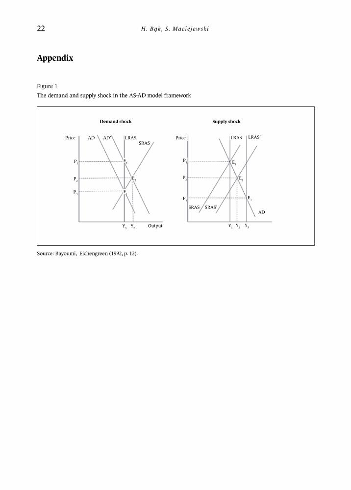
H. Bąk, S. Maciejewski22

Appendix

Figure 1The demand and supply shock in the AS-AD model framework

Demand shock Supply shock

Price PriceLRAS LRAS LRAS’SRAS

SRAS SRAS’

AD

AD

AD’

Output

P1E3

E2

E1

P2

P3

P1 E1

E2

E3

P2

P3

Y3 Y2Y3Y1 Y2

Source: Bayoumi, Eichengreen (1992, p. 12).

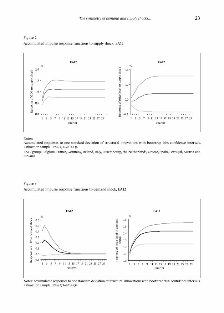
The symmetry of demand and supply shocks... 23

Figure 2Accumulated impulse response functions to supply shock, EA12

-0.2

0.0

0.2

0.4

1 3 5 7 9 11 13 15 17 19 21 23 25 27 29R

espo

nse

of p

rice

leve

l to

supp

ly sh

ock

quarter

EA12

0.0

0.5

1.0

1.5

2.0

1 3 5 7 9 11 13 15 17 19 21 23 25 27 29

Res

pons

e of

GD

P to

supp

ly sh

ock

quarter

EA12% %

Notes: Accumulated responses to one standard deviation of structural innovations with bootstrap 90% confidence intervals. Estimation sample: 1996 Q3−2014 Q4.EA12 group: Belgium, France, Germany, Ireland, Italy, Luxembourg, the Netherlands, Greece, Spain, Portugal, Austria and Finland.

Figure 3Accumulated impulse response functions to demand shock, EA12

-0.1

0.0

0.1

0.2

0.3

0.4

0.5

0.6

1 3 5 7 9 11 13 15 17 19 21 23 25 27 29 Res

pons

e of

GD

P to

dem

and

shoc

k

quarter

EA12

0.0

0.1

0.2

0.3

0.4

0.5

0.6

1 3 5 7 9 11 13 15 17 19 21 23 25 27 29

Res

pons

e of

pri

ce le

vel t

o de

man

d sh

ock

quarter

EA12

% %

Notes: accumulated responses to one standard deviation of structural innovations with bootstrap 90% confidence intervals. Estimation sample: 1996 Q3−2014 Q4.

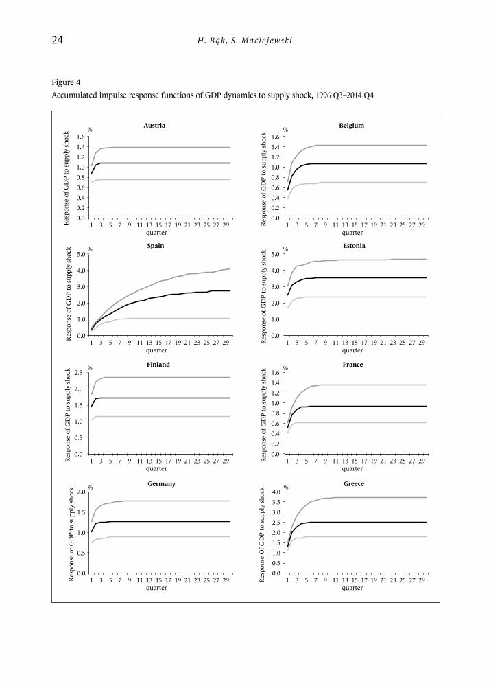
H. Bąk, S. Maciejewski24

Figure 4Accumulated impulse response functions of GDP dynamics to supply shock, 1996 Q3–2014 Q4

0.0 0.2 0.4 0.6 0.8 1.0 1.2 1.4 1.6

1 3 5 7 9 11 13 15 17 19 21 23 25 27 29 Res

pons

e of

GD

P to

supp

ly sh

ock

quarter

Austria

0.0 0.2 0.4 0.6 0.8 1.0 1.2 1.4 1.6

1 3 5 7 9 11 13 15 17 19 21 23 25 27 29 Res

pons

e of

GD

P to

supp

ly sh

ock

quarter

Belgium

0.0

1.0

2.0

3.0

4.0

5.0

1 3 5 7 9 11 13 15 17 19 21 23 25 27 29 Res

pons

e of

GD

P to

supp

ly sh

ock

quarter

Spain

0.0

1.0

2.0

3.0

4.0

5.0

1 3 5 7 9 11 13 15 17 19 21 23 25 27 29 Res

pons

e of

GD

P to

supp

ly sh

ock

quarter

Estonia

0.0

0.5

1.0

1.5

2.0

2.5

1 3 5 7 9 11 13 15 17 19 21 23 25 27 29 Res

pons

e of

GD

P to

supp

ly sh

ock

quarter

Finland

0.0 0.2 0.4 0.6 0.8 1.0 1.2 1.4 1.6

1 3 5 7 9 11 13 15 17 19 21 23 25 27 29 Res

pons

e of

GD

P to

supp

ly sh

ock

quarter

France

0.0

0.5

1.0

1.5

2.0

1 3 5 7 9 11 13 15 17 19 21 23 25 27 29 Res

pons

e of

GD

P to

supp

ly sh

ock

quarter

Germany

0.0 0.5 1.0 1.5 2.0 2.5 3.0 3.5 4.0

1 3 5 7 9 11 13 15 17 19 21 23 25 27 29 Res

pons

e O

f GD

P to

supp

ly sh

ock

quarter

Greece

% %

% %

% %

% %

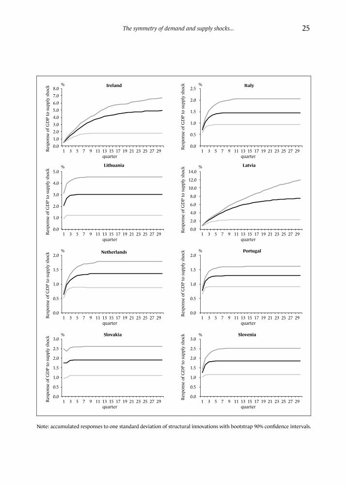
The symmetry of demand and supply shocks... 25

0.0 1.0 2.0 3.0 4.0 5.0 6.0

8.0 7.0

1 3 5 7 9 11 13 15 17 19 21 23 25 27 29 Res

pons

e of

GD

P to

supp

ly sh

ock

quarter

Ireland

0.0

0.5

1.0

1.5

2.0

2.5

1 3 5 7 9 11 13 15 17 19 21 23 25 27 29 Res

pons

e of

GD

P to

supp

ly sh

ock

quarter

Italy

0.0

1.0

2.0

3.0

4.0

5.0

1 3 5 7 9 11 13 15 17 19 21 23 25 27 29 Res

pons

e of

GD

P to

supp

ly sh

ock

quarter

Lithuania

0.0

2.0

4.0

6.0

8.0

10.0

12.0

14.0

1 3 5 7 9 11 13 15 17 19 21 23 25 27 29 Res

pons

e of

GD

P to

supp

ly sh

ock

quarter

Latvia

0.0

0.5

1.0

1.5

2.0

1 3 5 7 9 11 13 15 17 19 21 23 25 27 29 Res

pons

e of

GD

P to

supp

ly sh

ock

quarter

Netherlands

0.0

0.5

1.0

1.5

2.0

1 3 5 7 9 11 13 15 17 19 21 23 25 27 29 Res

pons

e of

GD

P to

supp

ly sh

ock

quarter

Portugal

0.0

0.5

1.0

1.5

2.0

2.5

3.0

1 3 5 7 9 11 13 15 17 19 21 23 25 27 29 Res

pons

e of

GD

P to

supp

ly sh

ock

quarter

Slovakia

0.0

0.5

1.0

1.5

2.0

2.5

3.0

1 3 5 7 9 11 13 15 17 19 21 23 25 27 29 Res

pons

e of

GD

P to

supp

ly sh

ock

quarter

Slovenia

% %

% %

% %

% %

Note: accumulated responses to one standard deviation of structural innovations with bootstrap 90% confidence intervals.

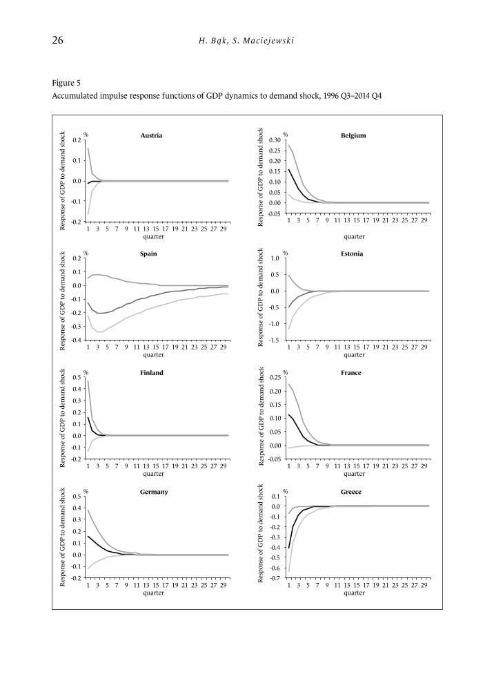
H. Bąk, S. Maciejewski26

Figure 5Accumulated impulse response functions of GDP dynamics to demand shock, 1996 Q3–2014 Q4

-0.2

-0.1

0.0

0.1

0.2

1 3 5 7 9 11 13 15 17 19 21 23 25 27 29 Res

pons

e of

GD

P to

dem

and

shoc

k

quarter

Austria

0.00

-0.05

0.10 0.15

0.25

0.05

0.20

0.30

1 3 5 7 9 11 13 15 17 19 21 23 25 27 29 Res

pons

e of

GD

P to

dem

and

shoc

k

quarter

Belgium

-0.4

-0.3

-0.2

-0.1

0.0

0.1

0.2

1 3 5 7 9 11 13 15 17 19 21 23 25 27 29 Res

pons

e of

GD

P to

dem

and

shoc

k

quarter

Spain

-1.5

-1.0

-0.5

0.0

0.5

1.0

1 3 5 7 9 11 13 15 17 19 21 23 25 27 29 Res

pons

e of

GD

P to

dem

and

shoc

k

quarter

Estonia

-0.2

-0.1

0.0

0.1

0.2

0.3

0.4

0.5

1 3 5 7 9 11 13 15 17 19 21 23 25 27 29 Res

pons

e of

GD

P to

dem

and

shoc

k

quarter

Finland

-0.05

0.00

0.05

0.10

0.15

0.20

0.25

1 3 5 7 9 11 13 15 17 19 21 23 25 27 29 Res

pons

e of

GD

P to

dem

and

shoc

k

quarter

France

-0.2

-0.1

0.0

0.1

0.2

0.3

0.4

0.5

1 3 5 7 9 11 13 15 17 19 21 23 25 27 29 Res

pons

e of

GD

P to

dem

and

shoc

k

quarter

Germany

-0.7 -0.6 -0.5 -0.4 -0.3 -0.2 -0.1 0.0 0.1

1 3 5 7 9 11 13 15 17 19 21 23 25 27 29

Res

pons

e of

GD

P to

dem

and

shoc

k

quarter

Greece

% %

% %

% %

% %

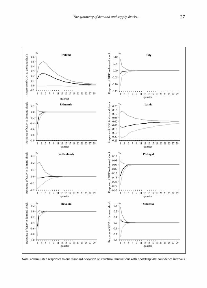
The symmetry of demand and supply shocks... 27

-0.1

0.0

0.1

0.2

0.3

0.4

0.5

0.6

1 3 5 7 9 11 13 15 17 19 21 23 25 27 29 Res

pons

e of

GD

P to

dem

and

shoc

k

quarter

Ireland

-0.15

-0.10

-0.05

0.00

0.05

0.10

1 3 5 7 9 11 13 15 17 19 21 23 25 27 29 Res

pons

e of

GD

P to

dem

and

shoc

k

quarter

Italy

-1.0

-0.8

-0.6

-0.4

-0.2

0.0

0.2

1 3 5 7 9 11 13 15 17 19 21 23 25 27 29 Res

pons

e of

GD

P to

dem

and

shoc

k

quarter

Lithuania

-0.25 -0.20 -0.15 -0.10 -0.05 0.00 0.05 0.10 0.15 0.20

1 3 5 7 9 11 13 15 17 19 21 23 25 27 29 Res

pons

e of

GD

P to

dem

and

shoc

k

quarter

Latvia

-0.2

-0.1

0.0

0.1

0.2

0.3

1 3 5 7 9 11 13 15 17 19 21 23 25 27 29 Res

pons

e of

GD

P to

dem

and

shoc

k

quarter

Netherlands

-0.30 -0.25 -0.20 -0.15 -0.10 -0.05 0.00 0.05 0.10

1 3 5 7 9 11 13 15 17 19 21 23 25 27 29 Res

pons

e of

GD

P to

dem

and

shoc

k

quarter

Portugal

-1.0

-0.8

-0.6

-0.4

-0.2

0.0

0.2

1 3 5 7 9 11 13 15 17 19 21 23 25 27 29 Res

pons

e of

GD

P to

dem

and

shoc

k

quarter

Slovakia

-0.3

-0.2

-0.1

0.0

0.1

0.2

0.3

1 3 5 7 9 11 13 15 17 19 21 23 25 27 29 Res

pons

e of

GD

P to

dem

and

shoc

k

quarter

Slovenia

% %

% %

% %

% %

Note: accumulated responses to one standard deviation of structural innovations with bootstrap 90% confidence intervals.

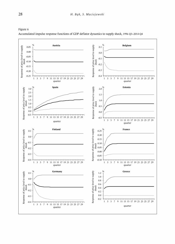
H. Bąk, S. Maciejewski28

Figure 6Accumulated impulse response functions of GDP deflator dynamics to supply shock, 1996 Q3−2014 Q4

-0.25

-0.20

-0.15

-0.10

-0.05

0.00

0.05

1 3 5 7 9 11 13 15 17 19 21 23 25 27 29 Res

pons

e of

pri

ce le

vel t

o su

pply

sh

ock

quarter

Austria

-0.4

-0.3

-0.2

-0.1

0.0

0.1

1 3 5 7 9 11 13 15 17 19 21 23 25 27 29

Res

pons

e of

pri

ce le

vel t

o su

pply

sh

ock

quarter

Belgium

-0.5 0.0 0.5 1.0 1.5 2.0 2.5 3.0

1 3 5 7 9 11 13 15 17 19 21 23 25 27 29

Res

pons

e of

pri

ce le

vel t

o su

pply

sh

ock

quarter

Spain

-0.5

0.0

0.5

1.0

1.5

2.0

1 3 5 7 9 11 13 15 17 19 21 23 25 27 29

Res

pons

e of

pri

ce le

vel t

o su

pply

sh

ock

quarter

Estonia

-0.4

-0.3

-0.2

-0.1

0.0

0.1

1 3 5 7 9 11 13 15 17 19 21 23 25 27 29 Res

pons

e of

pri

ce le

vel t

o su

pply

sh

ock

quarter

Finland

-0.10

-0.05

0.00

0.05

0.10

0.15

0.20

0.25

1 3 5 7 9 11 13 15 17 19 21 23 25 27 29

Res

pons

e of

pri

ce le

vel t

o su

pply

sh

ock

quarter

France

-0.4

-0.3

-0.2

-0.1

0.0

0.1

1 3 5 7 9 11 13 15 17 19 21 23 25 27 29 Res

pons

e of

pri

ce le

vel t

o su

pply

sh

ock

quarter

Germany

-0.2 0.0 0.2 0.4 0.6 0.8 1.0 1.2

1 3 5 7 9 11 13 15 17 19 21 23 25 27 29 Res

pons

e of

pri

ce le

vel t

o su

pply

sh

ock

quarter

Greece

% %

% %

% %

% %

The symmetry of demand and supply shocks... 29

Note: accumulated responses to one standard deviation of structural innovations with bootstrap 90% confidence intervals.

-1.0 -0.5 0.0 0.5 1.0 1.5 2.0 2.5 3.0 3.5

1 3 5 7 9 11 13 15 17 19 21 23 25 27 29

Res

pons

e of

pri

ce le

vel t

o su

pply

sh

ock

quarter

Ireland

-0.25 -0.20 -0.15 -0.10 -0.05 0.00 0.05 0.10 0.15

1 3 5 7 9 11 13 15 17 19 21 23 25 27 29

Res

pons

e of

pri

ce le

vel t

o su

pply

sh

ock

quarter

Italy

0.0

0.5

1.0

1.5

2.0

2.5

1 3 5 7 9 11 13 15 17 19 21 23 25 27 29

Res

pons

e of

pri

ce le

vel t

o su

pply

sh

ock

quarter

Lithuania

-2.0

0.0

2.0

4.0

6.0

8.0

10.0

1 3 5 7 9 11 13 15 17 19 21 23 25 27 29

Res

pons

e of

pri

ce le

vel t

o su

pply

sh

ock

quarter

Latvia

-0.4

-0.2

0.0

0.2

0.4

0.6

0.8

1 3 5 7 9 11 13 15 17 19 21 23 25 27 29

Res

pons

e of

pri

ce le

vel t

o su

pply

sh

ock

quarter

Netherlands

0.0

0.1

0.2

0.3

0.4

0.5

0.6

0.7

1 3 5 7 9 11 13 15 17 19 21 23 25 27 29

Res

pons

e of

pri

ce le

vel t

o su

pply

sh

ock

quarter

Portugal

-1.5 -1.0 -0.5 0.0 0.5 1.0 1.5 2.0 2.5

1 3 5 7 9 11 13 15 17 19 21 23 25 27 29

Res

pons

e of

pri

ce le

vel t

o su

pply

sh

ock

quarter

Slovakia

-0.4 -0.3 -0.2 -0.1 0.0 0.1 0.2 0.3 0.4

1 3 5 7 9 11 13 15 17 19 21 23 25 27 29

resp

onse

of p

rice

leve

l to

supp

ly

shoc

k

quarter

Slovenia

% %

% %

% %

% %

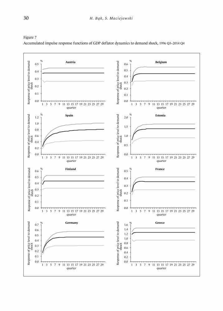
H. Bąk, S. Maciejewski30

Figure 7Accumulated impulse response functions of GDP deflator dynamics to demand shock, 1996 Q3−2014 Q4

0.0

0.1

0.2

0.3

0.4

0.5

1 3 5 7 9 11 13 15 17 19 21 23 25 27 29 Res

pons

e of

pri

ce le

vel t

o de

man

d sh

ock

quarter

Austria

0.0

0.1

0.2

0.3

0.4

0.5

0.6

1 3 5 7 9 11 13 15 17 19 21 23 25 27 29 Res

pons

e of

pri

ce le

vel t

o de

man

d sh

ock

quarter

Belgium

0.0

0.2

0.4

0.6

0.8

1.0

1.2

1 3 5 7 9 11 13 15 17 19 21 23 25 27 29 Res

pons

e of

pri

ce le

vel t

o de

man

d sh

ock

quarter

Spain

0.0

0.5

1.0

1.5

2.0

1 3 5 7 9 11 13 15 17 19 21 23 25 27 29 Res

pons

e of

pri

ce le

vel t

o de

man

d sh

ock

quarter

Estonia

0.0

0.1

0.2

0.3

0.4

0.5

0.6

1 3 5 7 9 11 13 15 17 19 21 23 25 27 29 Res

pons

e of

pri

ce le

vel t

o de

man

d sh

ock

quarter

Finland

0.0

0.1

0.2

0.3

0.4

0.5

1 3 5 7 9 11 13 15 17 19 21 23 25 27 29 Res

pons

e of

pri

ce le

vel t

o de

man

d sh

ock

quarter

France

0.0

0.1

0.2

0.3

0.4

0.5

0.6

0.7

1 3 5 7 9 11 13 15 17 19 21 23 25 27 29 Res

pons

e of

pri

ce le

vel t

o de

man

d sh

ock

quarter

Germany

0.0 0.2 0.4 0.6 0.8 1.0 1.2 1.4 1.6

1 3 5 7 9 11 13 15 17 19 21 23 25 27 29 Res

pons

e of

pri

ce le

vel t

o de

man

d sh

ock

quarter

Greece

% %

% %

% %

% %

The symmetry of demand and supply shocks... 31

0.0

0.5

1.0

1.5

2.0

1 3 5 7 9 11 13 15 17 19 21 23 25 27 29 Res

pons

e of

pri

ce le

vel t

o de

man

d sh

ock

quarter

Ireland

0.0

0.1

0.2

0.3

0.4

0.5

0.6

1 3 5 7 9 11 13 15 17 19 21 23 25 27 29 Res

pons

e of

pri

ce le

vel t

o de

man

d sh

ock

quarter

Italy

0.0

0.5

1.0

1.5

2.0

2.5

3.0

3.5

1 3 5 7 9 11 13 15 17 19 21 23 25 27 29 Res

pons

e of

pri

ce le

vel t

o de

man

d sh

ock

quarter

Lithuania

0.0

1.0

2.0

3.0

4.0

5.0

1 3 5 7 9 11 13 15 17 19 21 23 25 27 29 Res

pons

e of

pri

ce le

vel t

o de

man

d sh

ock

quarter

Latvia

0.0

0.2

0.4

0.6

0.8

1.0

1 3 5 7 9 11 13 15 17 19 21 23 25 27 29 Res

pons

e of

pri

ce le

vel t

o de

man

d sh

ock

quarter

Netherlands

0.0 0.1 0.2 0.3 0.4 0.5 0.6 0.7 0.8

1 3 5 7 9 11 13 15 17 19 21 23 25 27 29 Res

pons

e of

pri

ce le

vel t

o de

man

d sh

ock

quarter

Portugal

0.0 0.5 1.0 1.5 2.0 2.5 3.0 3.5 4.0

1 3 5 7 9 11 13 15 17 19 21 23 25 27 29 Res

pons

e of

pri

ce le

vel t

o de

man

d sh

ock

quarter

Slovakia

0.0

0.2

0.4

0.6

0.8

1.0

1.2

1 3 5 7 9 11 13 15 17 19 21 23 25 27 29 Res

pons

e of

pri

ce le

vel t

o de

man

d sh

ock

quarter

Slovenia

% %

% %

% %

% %

Note: accumulated responses to one standard deviation of structural innovations with bootstrap 90% confidence intervals.

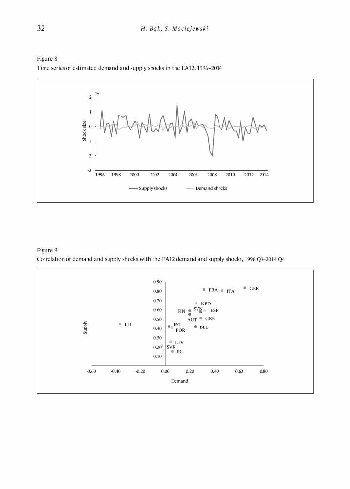
H. Bąk, S. Maciejewski32

Figure 8Time series of estimated demand and supply shocks in the EA12, 1996−2014

-31996 1998 2000 2002 2004 2006 2008 2010 2012 2014

-2

-1

0

1

2

Shoc

k si

ze

Supply shocks Demand shocks

%

Figure 9Correlation of demand and supply shocks with the EA12 demand and supply shocks, 1996 Q3−2014 Q4

AUTBEL

ESP

EST

FIN

FRA GER

GRE

IRL

ITA

LIT

LTV

NED

POR

SVK

SVN

0.10

0.20

0.30

0.40

0.50

0.60

0.70

0.80

0.90

-0.60 -0.40 -0.20 0.00 0.20 0.40 0.60 0.80

Supp

ly

Demand

The symmetry of demand and supply shocks... 33

Figure 10Correlation of demand and supply shocks with the EA12 demand and supply shocks, 1996 Q3−2008 Q4

AUTBEL

ESP

ESTFIN

FRA GER

GRE

IRL

ITA

LIT LTV

NED

POR

SVK

SVN

-0.40

0.20

0.40

0.60

0.80

1.00

-0.60 -0.40 -0.20 0.00 0.20 0.40 0.60 0.80 1.00

Supp

ly

Demand

-0.20

Figure 11Correlation of demand and supply shocks with the EA12 demand and supply shocks, 2010 Q1−2014 Q4

AUT

BELESP

EST

FIN

FRAGER

GRE

IRL

ITA

LIT

LTVNEDPOR

SVK

SVN

0.10

0.20

0.30

0.40

0.50

0.60

0.70

0.80

0.90

-0.60 -0.40 -0.20 0.00 0.20 0.40 0.60 0.80

Supp

ly

Demand

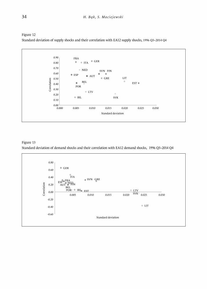
H. Bąk, S. Maciejewski34

Figure 12Standard deviation of supply shocks and their correlation with EA12 supply shocks, 1996 Q3−2014 Q4

AUT

BEL

ESP

EST

SVN FIN

FRAGER

GRE

IRL

ITA

LIT

LTV

NED

POR

SVK

0.00

0.10

0.20

0.30

0.40

0.50

0.60

0.70

0.80

0.90

0.000 0.005 0.010 0.015 0.020 0.025 0.030

Corr

elat

ion

Standard deviation

Figure 13Standard deviation of demand shocks and their correlation with EA12 demand shocks, 1996 Q3−2014 Q4

AUTBEL

ESP

EST

FINFRA

GER

SVN GRE

IRL

ITA

LIT

LTV

NED

PORSVK

-0.60

-0.40

-0.20

0.00

0.20

0.40

0.60

0.80

0.005 0.010 0.015 0.020 0.025 0.030Corr

elat

ion

Standard deviation

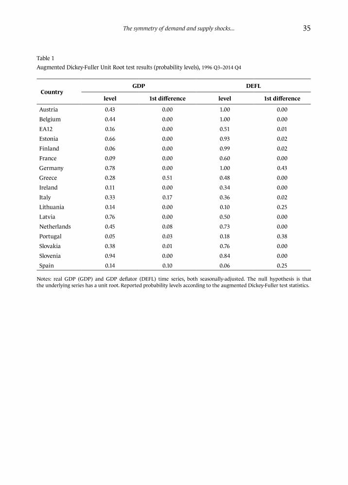
The symmetry of demand and supply shocks... 35

Table 1Augmented Dickey-Fuller Unit Root test results (probability levels), 1996 Q3−2014 Q4

CountryGDP DEFL

level 1st difference level 1st difference

Austria 0.43 0.00 1.00 0.00

Belgium 0.44 0.00 1.00 0.00

EA12 0.16 0.00 0.51 0.01

Estonia 0.66 0.00 0.93 0.02

Finland 0.06 0.00 0.99 0.02

France 0.09 0.00 0.60 0.00

Germany 0.78 0.00 1.00 0.43

Greece 0.28 0.51 0.48 0.00

Ireland 0.11 0.00 0.34 0.00

Italy 0.33 0.17 0.36 0.02

Lithuania 0.14 0.00 0.10 0.25

Latvia 0.76 0.00 0.50 0.00

Netherlands 0.45 0.08 0.73 0.00

Portugal 0.05 0.03 0.18 0.38

Slovakia 0.38 0.01 0.76 0.00

Slovenia 0.94 0.00 0.84 0.00

Spain 0.14 0.10 0.06 0.25

Notes: real GDP (GDP) and GDP deflator (DEFL) time series, both seasonally-adjusted. The null hypothesis is that the underlying series has a unit root. Reported probability levels according to the augmented Dickey-Fuller test statistics.

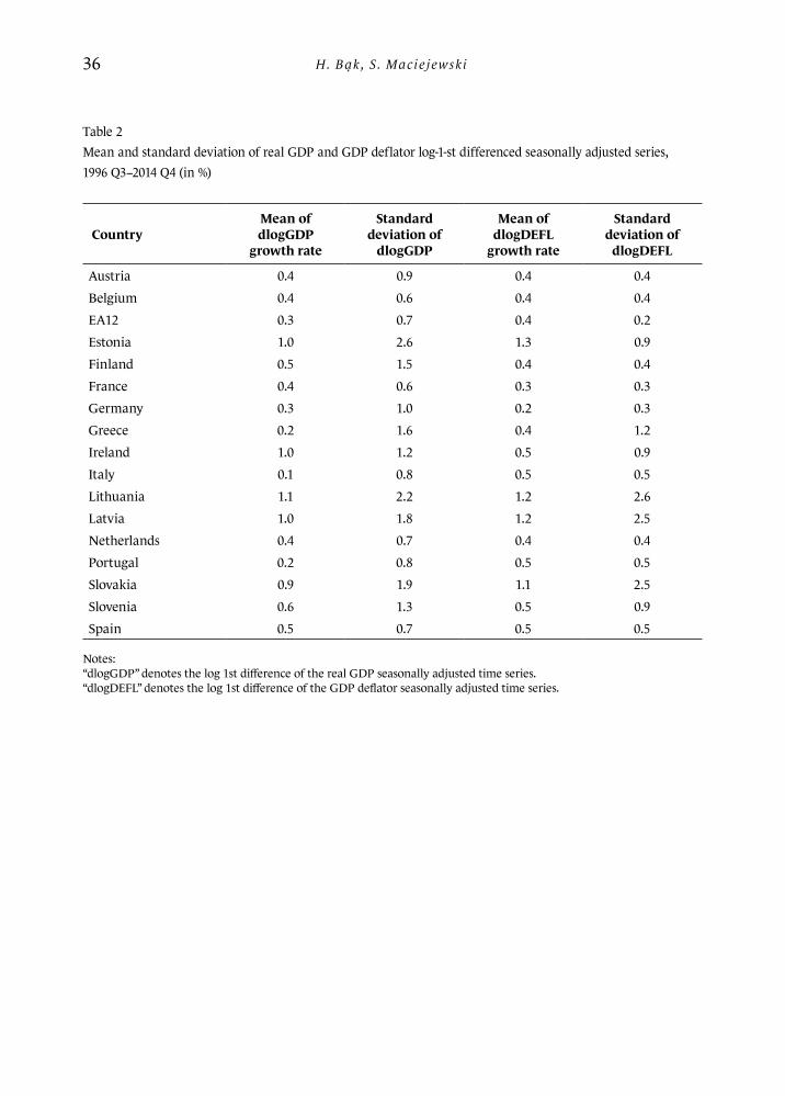
H. Bąk, S. Maciejewski36

Table 2Mean and standard deviation of real GDP and GDP deflator log-1-st differenced seasonally adjusted series, 1996 Q3−2014 Q4 (in %)

CountryMean of dlogGDP

growth rate

Standard deviation of

dlogGDP

Mean of dlogDEFL

growth rate

Standard deviation of

dlogDEFL

Austria 0.4 0.9 0.4 0.4

Belgium 0.4 0.6 0.4 0.4

EA12 0.3 0.7 0.4 0.2

Estonia 1.0 2.6 1.3 0.9

Finland 0.5 1.5 0.4 0.4

France 0.4 0.6 0.3 0.3

Germany 0.3 1.0 0.2 0.3

Greece 0.2 1.6 0.4 1.2

Ireland 1.0 1.2 0.5 0.9

Italy 0.1 0.8 0.5 0.5

Lithuania 1.1 2.2 1.2 2.6

Latvia 1.0 1.8 1.2 2.5

Netherlands 0.4 0.7 0.4 0.4

Portugal 0.2 0.8 0.5 0.5

Slovakia 0.9 1.9 1.1 2.5

Slovenia 0.6 1.3 0.5 0.9

Spain 0.5 0.7 0.5 0.5

Notes: “dlogGDP” denotes the log 1st difference of the real GDP seasonally adjusted time series. “dlogDEFL” denotes the log 1st difference of the GDP deflator seasonally adjusted time series.

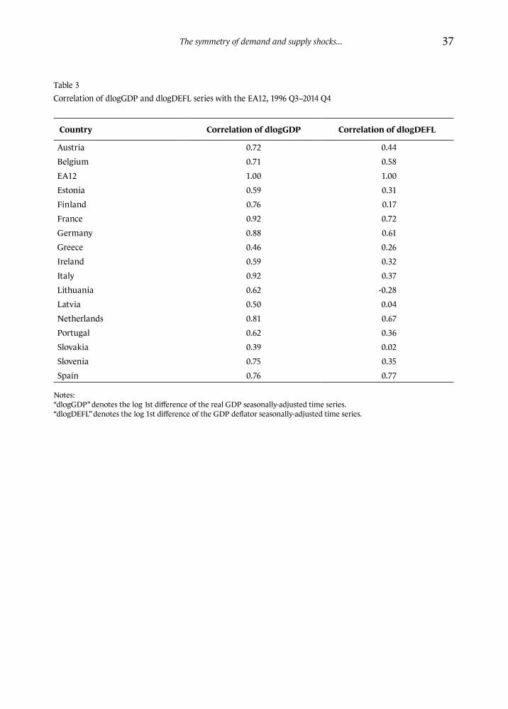
The symmetry of demand and supply shocks... 37

Table 3Correlation of dlogGDP and dlogDEFL series with the EA12, 1996 Q3−2014 Q4

Country Correlation of dlogGDP Correlation of dlogDEFL

Austria 0.72 0.44

Belgium 0.71 0.58

EA12 1.00 1.00

Estonia 0.59 0.31

Finland 0.76 0.17

France 0.92 0.72

Germany 0.88 0.61

Greece 0.46 0.26

Ireland 0.59 0.32

Italy 0.92 0.37

Lithuania 0.62 -0.28

Latvia 0.50 0.04

Netherlands 0.81 0.67

Portugal 0.62 0.36

Slovakia 0.39 0.02

Slovenia 0.75 0.35

Spain 0.76 0.77

Notes: “dlogGDP” denotes the log 1st difference of the real GDP seasonally-adjusted time series. “dlogDEFL” denotes the log 1st difference of the GDP deflator seasonally-adjusted time series.

H. Bąk, S. Maciejewski38

Table 4VAR lag order selection criteria, 1996 Q3−2014 Q4

CountryAkaike

information criterion

Schwarz information

criterion

Hannan-Quinn information

criterion

Austria 1 0 1

Belgium 2 1 2

EA12 4 1 4

Estonia 2 2 2

Finland 10 0 3

France 2 1 2

Germany 12 4 4

Greece 12 2 2

Italy 6 1 1

Ireland 8 1 6

Netherlands 8 1 2

Lithuania 2 0 0

Latvia 3 1 3

Portugal 12 0 3

Slovenia 2 0 1

Slovakia 0 0 0

Spain 4 2 4

Notes: lag orders indicated by the selected criterion.

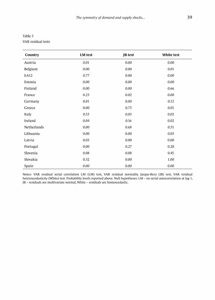
The symmetry of demand and supply shocks... 39

Table 5 VAR residual tests

Country LM test JB test White test

Austria 0.01 0.00 0.00

Belgium 0.00 0.00 0.01

EA12 0.77 0.00 0.00

Estonia 0.00 0.00 0.00

Finland 0.00 0.00 0.66

France 0.23 0.02 0.00

Germany 0.01 0.00 0.12

Greece 0.00 0.73 0.01

Italy 0.53 0.03 0.02

Ireland 0.04 0.16 0.02

Netherlands 0.00 0.68 0.51

Lithuania 0.00 0.00 0.03

Latvia 0.03 0.00 0.00

Portugal 0.00 0.27 0.28

Slovenia 0.08 0.08 0.45

Slovakia 0.32 0.00 1.00

Spain 0.00 0.00 0.00

Notes: VAR residual serial correlation LM (LM) test, VAR residual normality Jarque-Bera (JB) test, VAR residual heteroscedasticity (White) test. Probability levels reported above. Null hypotheses: LM − no serial autocorrelation at lag 1, JB − residuals are multivariate normal, White − residuals are homoscedastic.

H. Bąk, S. Maciejewski40

Table 6Variance decomposition of dlogGDP, 1996 Q3−2014 Q4

Country Period Forecast error Supply (%) Demand (%)

Austria1 0.0087 99.98 0.02

30 0.0089 99.96 0.04

Belgium1 0.0057 92.20 7.80

30 0.0065 92.81 7.19

EA121 0.0063 89.98 10.02

30 0.0072 90.55 9.45

Estonia1 0.0253 96.12 3.88

30 0.0263 95.54 4.46

Finland1 0.0147 98.89 1.11

30 0.0149 98.29 1.71

France1 0.0053 95.57 4.43

30 0.0060 95.77 4.23

Germany1 0.0103 97.74 2.26

30 0.0105 97.45 2.55

Greece1 0.0139 91.36 8.64

30 0.0159 91.11 8.89

Ireland1 0.0051 92.38 7.62

30 0.0125 98.14 1.86

Italy1 0.0069 99.90 0.10

30 0.0081 99.89 0.11

Lithuania1 0.0208 96.13 3.87

30 0.0221 94.72 5.28

Latvia1 0.0083 99.37 0.63

30 0.0182 99.86 0.14

Netherlands1 0.0063 99.89 0.11

30 0.0075 99.91 0.09

Portugal1 0.0078 97.25 2.75

30 0.0086 96.93 3.07

Slovakia1 0.0183 91.85 8.15

30 0.0189 86.47 13.53

Slovenia1 0.0124 99.81 0.19

30 0.0131 99.76 0.24

Spain 1 0.0040 90.41 9.5930 0.0074 96.07 3.93

Notes: ‘Forecast error’ denotes forecast error standard deviation of the dlogGDP for the given forecast horizon. Two last columns present percentage shares of each innovation (demand or supply shock) in the forecast variance.

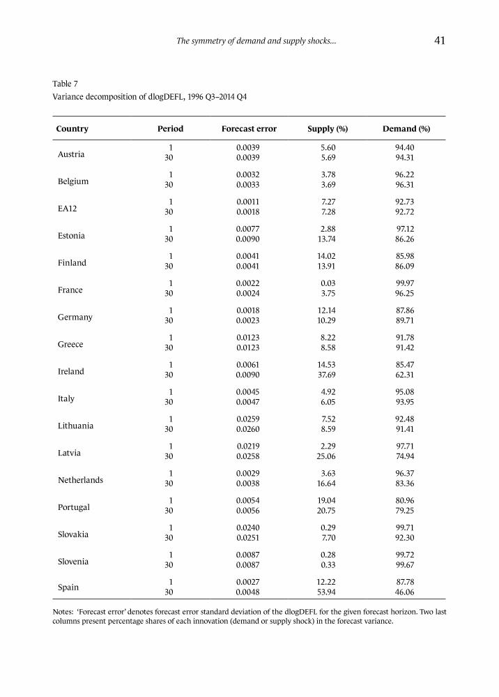
The symmetry of demand and supply shocks... 41

Table 7Variance decomposition of dlogDEFL, 1996 Q3−2014 Q4

Country Period Forecast error Supply (%) Demand (%)

Austria1 0.0039 5.60 94.40

30 0.0039 5.69 94.31

Belgium1 0.0032 3.78 96.22

30 0.0033 3.69 96.31

EA121 0.0011 7.27 92.73

30 0.0018 7.28 92.72

Estonia1 0.0077 2.88 97.12

30 0.0090 13.74 86.26

Finland1 0.0041 14.02 85.98

30 0.0041 13.91 86.09

France1 0.0022 0.03 99.97

30 0.0024 3.75 96.25

Germany1 0.0018 12.14 87.86

30 0.0023 10.29 89.71

Greece1 0.0123 8.22 91.78

30 0.0123 8.58 91.42

Ireland1 0.0061 14.53 85.47

30 0.0090 37.69 62.31

Italy1 0.0045 4.92 95.08

30 0.0047 6.05 93.95

Lithuania1 0.0259 7.52 92.48

30 0.0260 8.59 91.41

Latvia1 0.0219 2.29 97.71

30 0.0258 25.06 74.94

Netherlands1 0.0029 3.63 96.37

30 0.0038 16.64 83.36

Portugal1 0.0054 19.04 80.96

30 0.0056 20.75 79.25

Slovakia1 0.0240 0.29 99.71

30 0.0251 7.70 92.30

Slovenia1 0.0087 0.28 99.72

30 0.0087 0.33 99.67

Spain 1 0.0027 12.22 87.7830 0.0048 53.94 46.06

Notes: ‘Forecast error’ denotes forecast error standard deviation of the dlogDEFL for the given forecast horizon. Two last columns present percentage shares of each innovation (demand or supply shock) in the forecast variance.

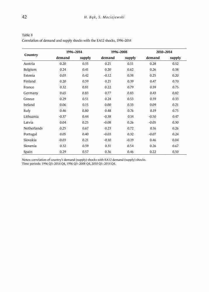
H. Bąk, S. Maciejewski42

Table 8Correlation of demand and supply shocks with the EA12 shocks, 1996−2014

Country1996−2014 1996−2008 2010−2014

demand supply demand supply demand supply

Austria 0.20 0.55 0.21 0.51 0.28 0.52

Belgium 0.24 0.41 0.20 0.62 0.26 0.38

Estonia 0.03 0.42 -0.12 0.38 0.25 0.20

Finland 0.20 0.59 0.21 0.39 0.47 0.70

France 0.32 0.81 0.22 0.79 0.59 0.75

Germany 0.65 0.83 0.77 0.83 0.43 0.82

Greece 0.29 0.51 0.24 0.53 0.59 0.33

Ireland 0.06 0.15 0.00 0.33 0.09 0.21

Italy 0.46 0.80 0.48 0.76 0.19 0.75

Lithuania -0.37 0.44 -0.38 0.14 -0.50 0.47

Latvia 0.04 0.25 -0.08 0.26 -0.05 0.30

Netherlands 0.25 0.67 0.23 0.72 0.16 0.26

Portugal 0.05 0.40 -0.03 0.32 -0.07 0.24

Slovakia -0.03 0.21 -0.10 -0.19 0.46 0.04

Slovenia 0.32 0.59 0.31 0.54 0.26 0.67

Spain 0.29 0.57 0.36 0.46 0.22 0.50

Notes: correlation of country’s demand (supply) shocks with EA12 demand (supply) shocks. Time periods: 1996 Q3−2014 Q4, 1996 Q3−2008 Q4, 2010 Q1−2014 Q4.

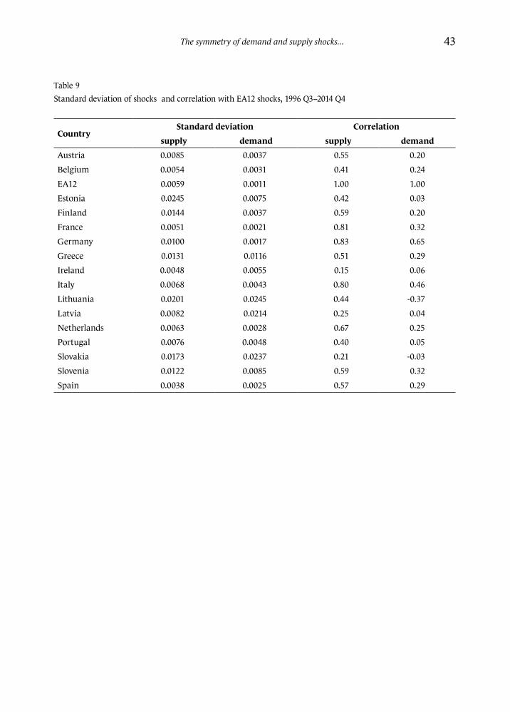
The symmetry of demand and supply shocks... 43

Table 9Standard deviation of shocks and correlation with EA12 shocks, 1996 Q3−2014 Q4

CountryStandard deviation Correlation

supply demand supply demand

Austria 0.0085 0.0037 0.55 0.20

Belgium 0.0054 0.0031 0.41 0.24

EA12 0.0059 0.0011 1.00 1.00

Estonia 0.0245 0.0075 0.42 0.03

Finland 0.0144 0.0037 0.59 0.20

France 0.0051 0.0021 0.81 0.32

Germany 0.0100 0.0017 0.83 0.65

Greece 0.0131 0.0116 0.51 0.29

Ireland 0.0048 0.0055 0.15 0.06

Italy 0.0068 0.0043 0.80 0.46

Lithuania 0.0201 0.0245 0.44 -0.37

Latvia 0.0082 0.0214 0.25 0.04

Netherlands 0.0063 0.0028 0.67 0.25

Portugal 0.0076 0.0048 0.40 0.05

Slovakia 0.0173 0.0237 0.21 -0.03

Slovenia 0.0122 0.0085 0.59 0.32

Spain 0.0038 0.0025 0.57 0.29