Embed Size (px)
Citation preview

Instructions for use
Title The use of geostationary satellite based rainfall estimation and rainfall-runoff modelling for regional flash floodassessment
Author(s) Suseno, Dwi Prabowo Yuga
Citation 北海道大学. 博士(工学) 甲第11130号
Issue Date 2013-09-25
DOI 10.14943/doctoral.k11130
Doc URL http://hdl.handle.net/2115/53880
Type theses (doctoral)
File Information Dwi_Prabowo_Yuga_Suseno.pdf
Hokkaido University Collection of Scholarly and Academic Papers : HUSCAP
THE USE OF GEOSTATIONARY SATELLITE
BASED RAINFALL ESTIMATION AND
RAINFALL-RUNOFF MODELLING FOR
REGIONAL FLASH FLOOD ASSESSMENT
Dwi Prabowo Yuga Suseno
Hokkaido University
2013
ii
THE USE OF GEOSTATIONARY SATELLITE BASED RAINFALL
ESTIMATION AND RAINFALL-RUNOFF MODELLING FOR
REGIONAL FLASH FLOOD ASSESSMENT
[静止衛星による観測データを用いた降雨推定手法と降雨流出モデル
による山地流域における突発的出水評価]
Dwi Prabowo Yuga Suseno
スセノ ドウィ プラボウオ ユガ
River and Watershed Engineering Laboratory
Faculty of Engineering
Hokkaido University
A dissertation submitted to the Graduate School of Engineering of the Hokkaido
University in partial fulfillment of the requirements for the degree of
Doctor of Engineering
August 2013

iii
…Kaaturaken kagem swargi Bpk Mulyono & Ibu Sugini…
اللھم اغفر لھم وارحمھم وعافھم واعف عنھم
(Dedicated to my late father and mother)
iv
ABSTRACT
The availability of rainfall triggered hazard information such as flash flood is crucial in the flood
disaster management and mitigation. However, providing that information is mainly hampered by
the shortage of data because of the sparse, uneven or absence the hydrological or meteorological
observation. Remote sensing techniques that make frequent observations with continuous spatial
coverage provide useful information for detecting the hydrometeorological phenomena such as
rainfall and floods. This study aims to develop and evaluate geostationary satellite based rainfall
estimation by considering cloud types and atmospheric environmental conditions. Furthermore,
the satellite rainfall estimation is coupled with rainfall-runoff model for regional flash flood
assessment.
First, a simple rainfall estimation method using geostationary satellite i.e. Multi-
functional Transport Satellite (MTSAT) blended with Tropical Rainfall Measuring Mission
(TRMM) 2A12 is performed for Java Island, Indonesia and its surrounding area. The blending
process is conducted by developing statistical relationship between cloud top temperature from
MTSAT 10.8µm channel (TIR1) which is collocated with rainfall rate (RR) acquired by TRMM
2A12. Inter comparison with TRMM Multi Precipitation Analysis (TMPA) data product is
conducted. Temporal validation result shows that TMPA demonstrated better statistical
performance than TIR1 and RR statistical relationship model. However for the spatial correlation,
TIR1 and RR statistical relationship model shows reasonably better performance than TMPA.
Second, the rainfall estimation method basically uses an assumption the lower cloud top
temperature is associated with heavier rainfall, particularly for convective cloud type. To fulfill
such assumption, the statistical relationship is developed mainly for cumulonimbus (Cb) cloud
type. A new two-dimensional threshold diagram (2D-THR) has been developed based on
maximum likelihood cloud classification results, which can readily be applied for MTSAT split
window datasets. The study area is Japan and its surrounding area. By integrating the cloud type
classification especially by separating Cb cloud type from other cloud types can improve the TIR1
and RR statistical relationship, which is indicated by increasing correlation coefficient and the
gradient of regression line. Therefore, underestimating rainfall intensity can be avoided by
applying rainfall rate and cloud top temperature relationship that uses Cb cloud type only rather
than using all cloud types. A good agreement between estimated and measured storm rainfall also
has been demonstrated when use this approach.
The geostationary satellite based rainfall estimation then applied for characterizing the
storm severity. The Hosking-Wallis Regional Frequency Analysis (HW-RFA) method is used to
v
define the frequency distribution of long-term hourly maximum rainfall over Hokkaido Island.
HW-RFA indicates that Generalized Normal/Log Normal three parameters (GNO/LN3) is
suitable to describe the frequency distribution of long-term hourly maximum rainfall over
Hokkaido Island. A return period map during heavy rainfall event is generated by using MTSAT
based rainfall estimation, based on the GNO/LN3 distribution. A comparison with AMeDAS
return period of the same rainfall even demonstrates that that the return period information shown
by MTSAT rainfall is comparable with AMeDAS rainfall return period. For assessing the return
period of an extreme event in the area that observed rainfall is lacking, the use of geostationary
satellite based is proved useful to overcome such problem.
Third, total Precipitable Water Vapor (PWV) as a product of Global Positioning System
observation and atmospheric vertical instability were considered to represent the atmospheric
environmental conditions during the development of TIR1 and RR statistical models. The results
demonstrated that the models that considered the combination of total PWV and atmospheric
vertical instability were relatively more sensitive to heavy rainfall than were the models that
considered no atmospheric environmental conditions. Intercomparison results with the TRMM
3B42 rainfall estimation product confirmed that MTSAT-based rainfall estimations made by
considering atmospheric environmental conditions were more accurate for estimating rainfall
generated by Cb cloud.
Lastly, a regional flash flood assessment is conducted based on two rainfall-runoff
models: (i) empirical regression model approach and (ii) physical based approach using
land surface model. The empirical model uses the multiple regression approach to draw a
relationship between the flash flood severity and hydrological, morphometrical and
meteorological conditions. Particularly for flash flood severity related to hydrological
condition the statistical relationship is strongly determined by initial soil moisture
condition. The resulted empirical models shows that flash flood severity as the function of
morphometrical factors can provide flash flood potential information. Moreover, flash
flood severity as the function of hydrological and meteorological factors demonstrate
more dynamic pattern since they are related to rainfall intensity distribution. The physical
based approach for flash flood assessment had been conducted by implementing river
flow simulation the minimal advance treatments of surface interaction and runoff
(MATSIRO). The result indicates that the river flow simulated by MTSAT downscaled
with relatively sparse rainfall observation is comparable with the river flow simulation
using more dense rain observation network.

vi
静止衛星による観測データを用いた降雨推定手法と降雨流出モデルによる山地
流域における突発的出水評価
突発的出水をもたらす豪雨の早期探知は洪水による被害を低減させる上で不可欠であるが,山
地流域では現地観測データが乏しいという現状にある. これに対してリモートセンシング技術の
利用は高い時空間解像度での観測を可能とし, 降雨流出機構を解明及び予測する上で有用な手段
となり得る. 本研究は静止衛星による観測データを用いた雲分類手法と大気の環境場を考慮した
降雨強度推定手法を提案し, 得られた降雨データと降雨流出モデルを併せた山地流域における突
発的出水の危険度の評価を実施するものである.
まず MTSAT(Multi-functional Transport Satellite)と同じく人工衛星である TRMM(Tropical
Rainfall Measuring Mission) 2A12 の観測データによる降雨強度の推定精度の評価をインドネシ
アの Java 島と周辺地域を対象に実施した. ここで使用される降雨強度推定手法は MTSAT によっ
て観測される 10.8μm の近赤外放射データが示す雲頂温度と TRMM による降雨強度(TMPA; TRMM
Multi Precipitation Analysis)の統計的関係を用いるものである. 得られた結果の妥当性とし
て, MTSAT による雲頂温度情報に基づく降雨データは TMPA と同程度の精度を有することがわかっ
た.
豪雨は一般に雲頂高度が高くその温度が低い積乱雲によってもたらされる. そこで積乱雲に
特化し, 積乱雲のみの雲頂温度と降雨量の統計的関係から新たに降雨強度を推定する手法を開発
した. 積乱雲の抽出には MTSAT により観測される 2つの異なる波長帯を使用し, split window 法
と最尤法を組み合わせることによって雲分類ダイアグラムを作成し, 積乱雲の抽出を可能とした.
本手法によって抽出された積乱雲の雲頂温度と降雨量との統計的関係はすべての雲を扱った場合
の統計的関係よりも高い相関を示すことが確認された. また, 得られた降雨データを現地観測デ
ータと比較したところ高い一致が見られた.
上記で開発した積乱雲に特化した降雨強度推定手法を用いて豪雨の発生確率年の評価を行っ
た. ここで使用したのは Hosking & Wallis によって提案されている HW-RFA (Hosking and
Wallis Regional Frequency Analysis)である.同手法を北海道に適用し, 年最大時間降雨強度に
着目した発生確率年評価を実施したところ, 著者によって作成された降雨データと AMeDAS
(Automated Meteorological Data Acquisition System)降雨データによる豪雨の発生確率年の空
間分布は類似するものであった. この結果は現地観測データの乏しい流域において高い時空間ス
ケールで豪雨の確率年評価が議論可能であり, その入力値として著者が開発した降雨強度推定手
法による降雨データが有用であることを示すものである.
次に降雨強度の推定に関し, 雲頂温度に加え GPS (Global Positioning System)観測によって
得られる可降水量と領域気象モデルによる大気の鉛直不安定度の効果を加味した降雨強度推定手
法を新たに開発した. その結果,可降水量と鉛直不安定度の大きさは豪雨を捉える上で不可欠な
要素であり, 雲頂温度に加えこれら 2項目を考慮することによって, より高い精度で豪雨の検知
が可能であることが TRMM (3B42)降雨データとの比較によって示された.
最後に著者によって開発された降雨強度推定手法を降雨流出モデルに適用することで山地流
域を対象とした突発的出水の危険度の評価を実施した. 降雨流出モデルは(i)水文, 気象, 地形
等の流域特性により構成される経験的モデルと(ii)陸面過程モデルの 2種類を対象とした. 降雨
イベントごとに総降雨量と損失雨量関係に着目した分析を行ったところ, 突発的出水の危険度は
流域が降雨直前に飽和状態に近い場合であれば地形特性によって説明されやすいとの結果が得ら
れた. 一方, 水文気象要素によって決定される突発的出水危険度は降雨パターンに依存するため
動的に振る舞う特徴を有する. 一方, 陸面過程モデルを用いた物理的アプローチに関しては植生
による蒸発散やグリッド内の地形特性を考慮した MATSIRO (Minimal Advanced Treatments of
Surface Interaction and RunOff)を石狩川流域に適用できるように修正し, 利用可能とした.
その結果, 本研究において提案した降雨強度推定手法による降雨データを MATSIRO に与えること
で得られるピーク流量は現地観測による降雨データを使用した場合と高い一致が見られた.以上
より, 本研究は現地観測データの乏しい流域における突発的出水の評価を行う上でリモートセン
シング技術の多角的及び高度利用の有用性を示した.
vii
ACKNOWLEGMENTS
Praise be to Allah SWT, the Cherisher and Sustainer of the Worlds. I owe my deepest gratitude to many persons, who support me from the very beginning of my
study. Since it is difficult to memorize all of them, I would like to apologize to any persons, I forget to mention.
First, I would like to express my deepest and sincere gratitude to my supervisor, Associate Prof. Dr. Tomohito J. Yamada for his supports, guidance and encouragements through out my study. I wish to express my sincere gratitude Prof. Norihiro Izumi as my co-supervisor and head of River and Watershed Engineering Laboratory (RWE Lab) for providing an opportunity to this study. I am also indebted to Dr. Hiroshi Hayasaka who gives me chance to study in Hokkaido University. I extend my sincere thanks to Prof. Takafumi Sugiyama, Prof. Yasuyuki Shimizu, Prof. Toshihiko Yamashita, Prof. Hiroyuki Tanaka, Prof. Hiroshi Yokota, Prof. Shunji Kanie, Prof. Toru Tamura, Prof. Takashi Nakatsuji, Dr. Ichiro Kimura and Dr. Yasunori Watanabe as the committee member. My appreciation goes to Dr. Yadu Pokhrel, Dr. Suichi Kure for their kind attentions and supports for my study.
I would like to express my sincere thanks for Ministry of Forestry Republic of Indonesia (my employee), particularly Watershed Management Office of Indragiri Rokan at Pekanbaru, Riau, that give me permission to pursue my doctoral degree. I indebted to some Geography Faculty members at Gadjah Mada University, Yogyakarta, Indonesia (Prof. Dr. Hartono, DESS, Dr. Projo Danudoro, M.Sc, Prof. Dr. Junun Sartohadi, M.Sc, Dr. Pramono Hadi, M.Sc, Dr. Suharyadi, M.Sc) and the Faculty of Geoinformation Science and Earth Observation members, University of Twente, Enschede, The Netherlands (Dr. Ben Maathuis, Dr. Christ Mannaerts).
My sincere gratitude goes to E3 (Dr. Werawan Menakul, Mifue Shimamura), International Affairs Office of Engineering member (Yuki Tsuji, Kyoko Kawamura), RWE Lab Secretary (Sayo Uyama, Numata Nozomi).
I extend my sincere thank for Ministry of Education, Culture, Sports, Science and Technology (MEXT) for financial support. My study also partially supported by the Research Program on Climate Change Adaptation, Ministry of Education, Culture, Sports, Science and Technology, Japan (RECCA/MEXT), the MEXT SOUSEI program (theme C-i-C) the Integrated Study Project on Hydro-Meteorological Prediction and Adaptation to Climate Change in Thailand (IMPAC-T), the Science and Technology Research Partnership for Sustainable Development, the JST-JICA, Japan and Core Research for Evolutional Science and Technology program (CREST/JST). My sincere thank goes to Hitachi Zosen Corporation for providing an immense number of reliable datasets of GPS precipitable water.
I am grateful to the past and present RWE Lab members: Takuya Wada, Yuta Nakayama, Junya Nagahara, Yoshihiro Hata, Aoki Akinori, Kouki Wachi, Dr. Atinkut, Daham, Hossein, Takenori Kouno, Jun Sasaki, Yamahara Kouki, Dr. Adriano, Intan, Shenouda, Jeramee, Haruka Kuse, Kensuke Naito, Takahiro Ohyama, Kazunori Takahashi, Taiki Fukushima, Watanabe Yamato, Aiko Tokugawa, Yoshikazu Kitano, Daisuke Kamada, Jahir Uddin, Dr. Murad Farukh.
My sincere thanks go to all Indonesian students and families who live in Sapporo city, for their friendliness and hospitality. I am sorry not to mention you by name; however I have to express my special thanks to Eko Siswoyo and Dr. Erianto Indra Putra who help me to open my way to study in Hokudai.
I would like to extent my sincere gratitude to my parents in law, my brothers and sister (Mas Bambang, Widi, Catur), my brothers and sisters in law (Mas Yudhi, Mbak Lela, Mbak Sri, Mas Nano, Mas Pram, Mbak Hesti, Mas Puja, Mbak Nining) for your constant support and do’a.
Last but not least, my sincerely grateful for my wife Endar for your patience, encouragement, trust and most of all your love. You leave your job for accompany and support me in Sapporo, I really appreciate it. My sincere thank also goes to my lovely daughters Assyifa and Harumi. I am very proud of both of you.
Dwi Prabowo Yuga Suseno

viii
TABLE OF CONTENTS
ABSTRACT .................................................................................................................................... iv ACKNOWLEGMENTS.................................................................................................................vii TABLE OF CONTENTS ..............................................................................................................viii LIST OF FIGURES.......................................................................................................................... x LIST OF TABLES ........................................................................................................................xiii Chapter 1. GENERAL INTRODUCTION.......................................................................................1
1.1. BACKGROUND ............................................................................................................ 2 1.2. RESEARCH OBJECTIVES ........................................................................................... 3 1.3. STRUCTURE OF THE DISSERTATION.....................................................................4
Chapter 2. GEOSTATIONARY SATELLITE BASED RAINFALL ESTIMATION AND VALIDATION ................................................................................................................................. 6
Abstract ........................................................................................................................................ 7 2.1. INTRODUCTION ..........................................................................................................8 2.2. THE STUDY AREA AND DATASETS........................................................................9 2.3. METHOD AND VALIDATION SCHEMES............................................................... 10
2.3.1. The blending process through TIR1 and RR statistical relationship ...................... 10 2.3.2. Validation Schemes and Statistical Analysis ....................................................... 12
2.4. RESULTS AND DISCUSSIONS................................................................................. 14 2.4.1. Temporal validation ............................................................................................. 14 2.4.2. Spatial validation..................................................................................................15
2.5. SUMMARY AND CONCLUSIONS ........................................................................... 17 Chapter 3. REMOTE SENSING BASED CLOUD TYPE CLASSIFICATION FOR SUPPORTING RAINFALL ESTIMATION ................................................................................. 18
Abstract ...................................................................................................................................... 19 3.1. INTRODUCTION ........................................................................................................20 3.2. STUDY AREA AND DATA........................................................................................ 22 3.3. METHODS ................................................................................................................... 22
3.3.1. The development of 2D-THR based cloud type classification............................. 22 3.3.2. Validation of 2D-THR based cloud type classification........................................ 25 3.3.3. Integration of 2D-THR based cloud type classification into statistical based rainfall estimation. ................................................................................................................. 26
3.4. RESULTS AND DISCUSSION ................................................................................... 27 3.4.1. The 2D-THR based cloud type classification result and its validation. ...............27 3.4.2. Implementation of cloud type classification for statistical based rainfall estimation............................................................................................................................... 31
3.5. SUMMARY AND CONCLUSIONS ........................................................................... 32 Chapter 4. THE USE OF GEOSTATIONARY BASED RAINFALL ESTIMATION FOR CHARACTERIZING STORM SEVERITY.................................................................................. 34 Abstract .......................................................................................................................................... 35
4.1. INTRODUCTION ........................................................................................................36 4.2. STUDY AREA AND DATA........................................................................................ 37 4.3. METHODS ................................................................................................................... 38
4.3.1. Satellite rainfall estimation...................................................................................38 4.3.2. Regional Frequency Analysis............................................................................... 39
4.4. RESULTS AND DISCUSSIONS................................................................................. 41 4.4.1. Rainfall estimation based on BT and RR statistical relationship .........................41 4.4.2. RFA of Hokkaido Island ...................................................................................... 43 4.4.3. Strom severity characterization by return period mapping .................................. 46
4.5. SUMMARY AND CONCLUSIONS ........................................................................... 48 Chapter 5. INTEGRATION OF ATMOSPHERIC ENVIRONMENTAL CONDITIONS INTO GEOSTATIONARY SATELLITE BASED RAINFALL ESTIMATION .................................... 50
ix
Abstract .......................................................................................................................................... 51 5.1. INTRODUCTION ........................................................................................................52 5.2. STUDY AREA AND MATERIALS ............................................................................ 53 5.3. METHODS ................................................................................................................... 54
5.3.1. Parallax correction for geostationary satellite image ...........................................54 5.3.2. Statistical model development by considering atmospheric conditions ............... 54
5.4. RESULTS AND DISCUSSION ................................................................................... 57 5.5. SUMMARY AND CONCLUSIONS ........................................................................... 66
Chapter 6. EMPIRICAL REGRESSION BASED RAINFALL-RUNOFF MODEL FOR FLASH FLOODS SEVERITY ASSESSMENT.......................................................................................... 68 Abstract .......................................................................................................................................... 69
6.1. INTRODUCTION ........................................................................................................70 6.2. THE STUDY AREA AND DATASETS......................................................................71 6.3. METHODS ................................................................................................................... 72
6.3.1. Flash flood severity identification ........................................................................ 72 6.3.2. Hydrological Characterization.............................................................................. 73 6.3.3. Morphometrical Characterization.........................................................................75 6.3.4. Catchments Meteorology Characterization ..........................................................76 6.3.5. Multiple regression analysis ................................................................................. 77
6.4. RESULTS AND DISCUSSIONS................................................................................. 78 6.4.1. Flash flood severity analysis ................................................................................ 78 6.4.2. Morphometrical characteristics ............................................................................79 6.4.3. Hydrological characteristics ................................................................................. 81 6.4.4. Meteorological characteristics.............................................................................. 84 6.4.5. Flash flood severity index development and implementation. .............................85
6.5. SUMMARY AND CONCLUSIONS ........................................................................... 87 Chapter 7. PHYSICAL BASED RAINFALL-RUNOFF MODEL FOR FLASH FLOODS ESTIMATION................................................................................................................................ 89 Abstract .......................................................................................................................................... 90
7.1. INTRODUCTION ........................................................................................................91 7.2. THE STUDY AREA AND DATASETS......................................................................92 7.3. DESCRIPTION OF THE MATSIRO LAND SURFACE MODEL............................. 95 7.4. METHOD...................................................................................................................... 98
7.4.1. DEM processing for the topographic and river network parameters extraction...98 7.4.2. Land surface parameters data handling ................................................................99 7.4.3. Atmospheric data forcing preparation and statistical downscaling ......................99 7.4.4. River flow simulation schemes ..........................................................................101
7.5. RESULTS AND DISCUSSIONS............................................................................... 101 7.5.1. The MATSIRO data forcing acquisition and preparation using remote sensing and GIS 101 7.5.2. Comparison of river flow simulation results vs. observed river flow ................ 104
7.6. SUMMARY AND CONCLUSIONS ......................................................................... 109 Chapter 8. SUMMARY, CONCLUSIONS AND RECOMMENDATIONS............................... 110
8.1. SUMMARY AND CONCLUSIONS ......................................................................... 111 8.2. RECOMMENDATIONS ............................................................................................ 117
REFERENCES............................................................................................................................. 118 APPENDICES.............................................................................................................................. 126 CURRICULUM VITAE ..............................................................................................................137 LIST OF PUBLICATIONS..........................................................................................................138
x
LIST OF FIGURES
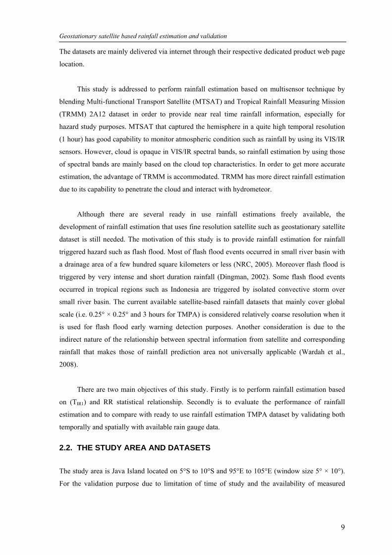
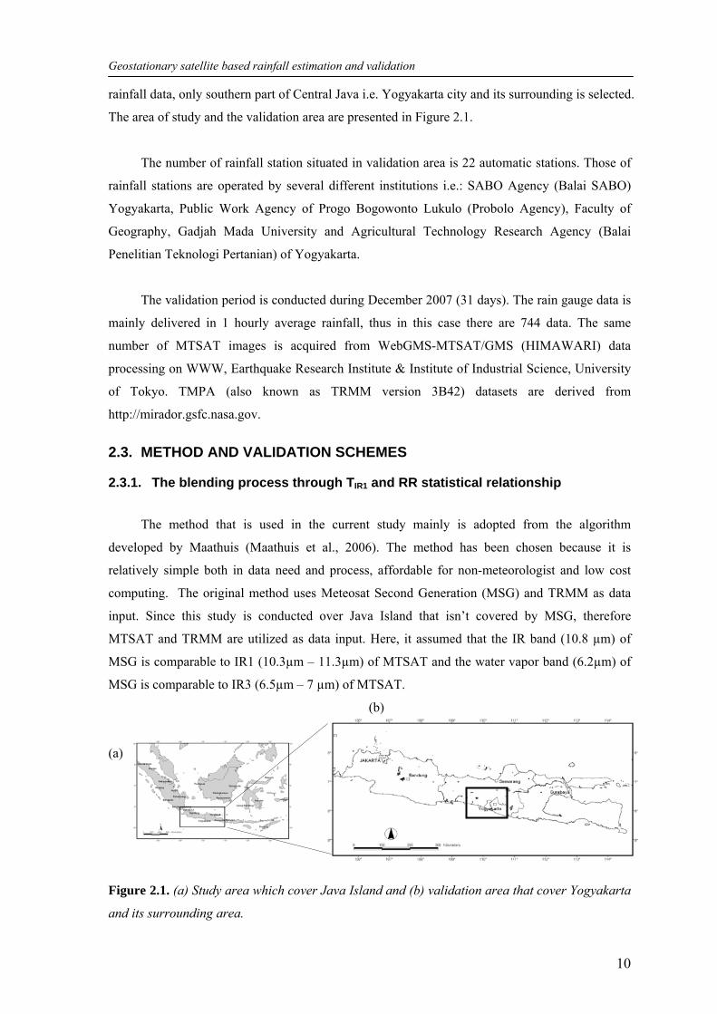
Figure 1.1. Outline of the dissertation ............................................................................................. 5 Figure 2.1. (a) Study area which cover Java Island and (b) validation area that cover Yogyakarta
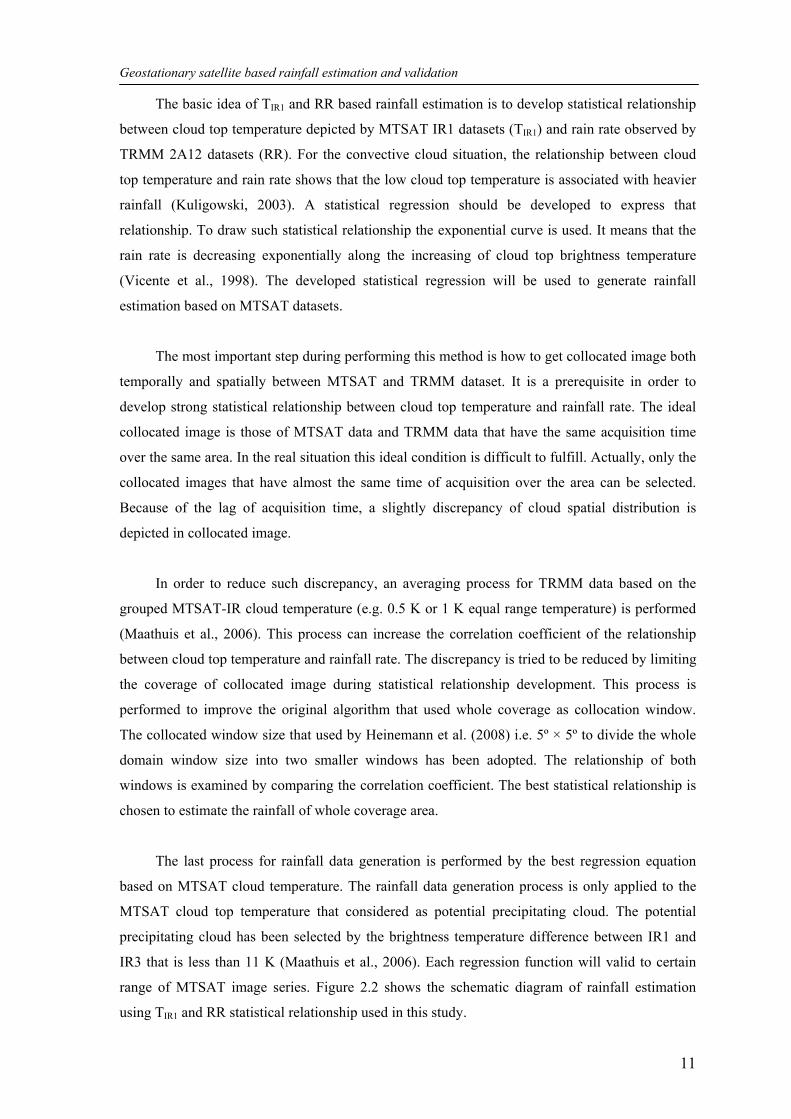
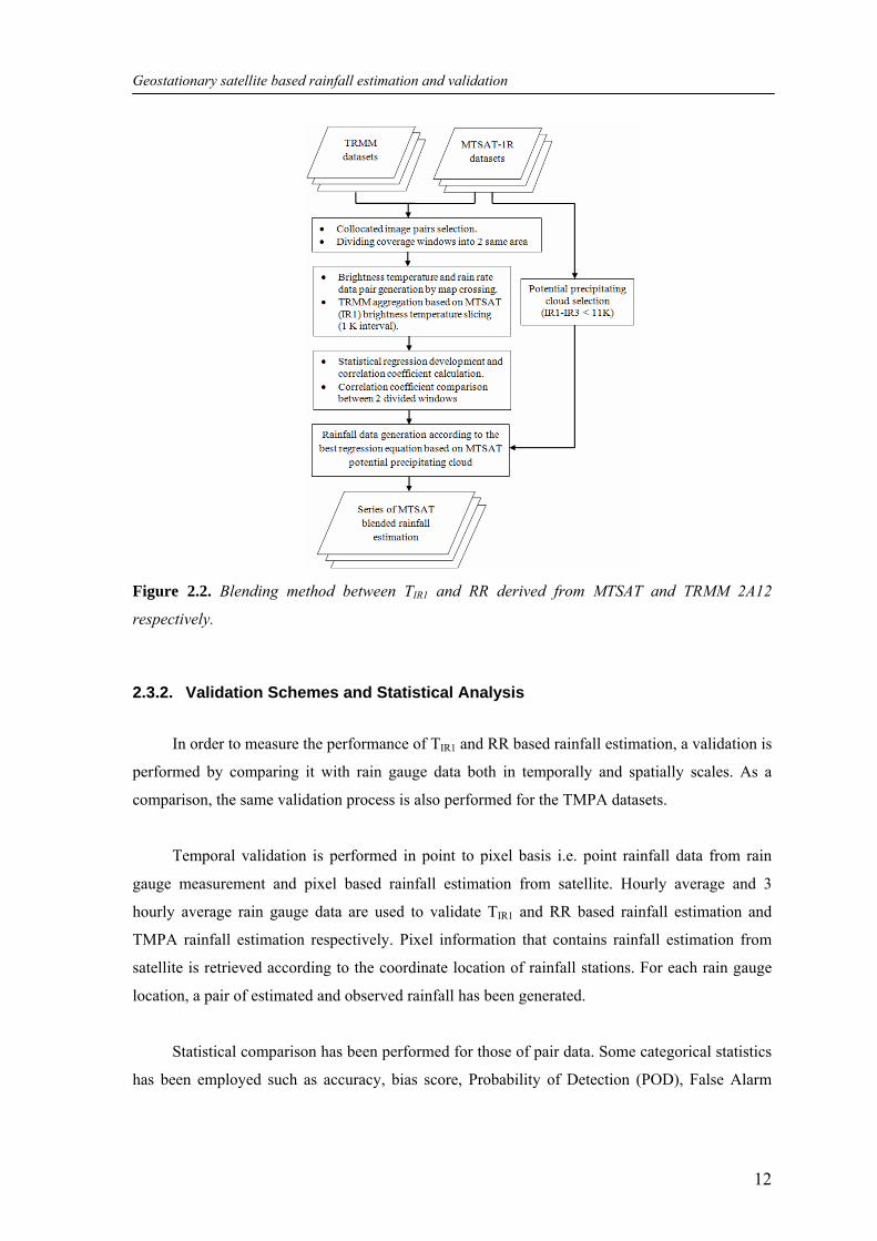
and its surrounding area. ........................................................................................................ 10 Figure 2.2. Blending method between TIR1 and RR derived from MTSAT and TRMM 2A12
respectively. ........................................................................................................................... 12 Figure 2.3. Comparison of correlation coefficient of the collocated images.................................14 Figure 3.1. Spectral characteristics of ice and water cloud (Kerkmann, 2004) .............................21 Figure 3.2. Comparison of Khat values between JMA vs. MAX and JMA vs. NN for selected
images during JJAS 2010. ..................................................................................................... 24 Figure 3.3. (a) A scatter plot of mean centre of each cloud type derived from MAX classification
results; (b) 2D-THR for cloud-type classification by using TIR1 and ΔTIR1-IR2 of MTSAT 1R................................................................................................................................................ 25
Figure 3.4. (a) Cloud-type classification result obtained using 2D-THR algorithm and (b) its corresponding night-time microphysical color composite for 2 August 2009 at 02:30 UTC................................................................................................................................................ 28
Figure 3.5. Inter-comparison of the reclassified cloud type classification between (a) 2D-THR cloud type classification result and (b) the JMA product for 2 August 2009 02:30 UTC. 2D-THR is resampled into the same spatial resolution as JMA. ................................................. 29
Figure 3.6. Hourly variation in the spatial correlation of Cb ((a) and (e)), HC ((b) and (f)), MC ((c) and (g)) and LC ((d) and (h)) percentage between 2D-THR and JMA cloud classification for tropical region ((a)–(d)) and subtropical region ((e)–(h)) during June, July, August and September 2009. .................................................................................................................... 30
Figure 3.7. Comparison of statistical regression of Tb and RR for several storm rainfall events by considering only Cb cloud (solid regression line) and by including all type of clouds in June 2010. ...................................................................................................................................... 31
Figure 4.1. The study area shows Japan area and its surrounding. The dashed line is AMeDAS C-band radar network coverage boundary................................................................................. 37
Figure 4.2. MTSAT based rainfall estimation and return period mapping methodology used in this study................................................................................................................................ 38
Figure 4.3. Cloud top brightness temperature and rainfall rate statistical relationship of storm rainfall events during June – September 2010 over Japan and its surrounding. ....................42
Figure 4.4. (a) Strom rainfall estimation distributions over Kyushu Island on 22 June 2010 at 11:30UTC; (b) rainfall distribution at the same location and time derived by spatial interpolation of point rain gauge measurement. .................................................................... 43
Figure 4.5. (a) Interpolation map of average of long-term maximum yearly rainfall (1-hour duration) by IDW method; (b) shaded relief map represents the topography of Hokkaido Island. The dashed line shows the boundary of the western region (Sub Region A) and eastern region (Sub Region B)............................................................................................... 43
Figure 4.6. (a) and (c) discordancy diagram for western and eastern region respectively which represent discordant stations (D > 3) (denoted by red triangle). (b) and (d) discordancy diagram for western and eastern region respectively after removing discordant stations which are use for determining frequency distribution. ..........................................................44
Figure 4.7. Identification of regional frequency distribution using HW-RFA moment ratio LCs LCk diagram for (a) western region and (b) eastern region of Hokkaido Island..................45
Figure 4.8. Cumulative distribution function of GNO/LN3 distribution for (a) Sub Region A and (b) Sub Region B. .................................................................................................................. 46
Figure 4.9. Spatial distribution of 3-hour average rainfall intensity (mm/h) from derived from C-band AMeDAS rainfall radar over Hokkaido Island on 24 August 2010 at 01:30 – 04:30 UTC (Yamada et al., 2012).................................................................................................... 46
Figure 4.10. Daily weather map that showing frontal system over Japan and its surrounding area on (a) 23 August 2010 and (b) 24 August 2010 (JMA, 2010). .............................................. 47
xi
Figure 4.11. (a) MTSAT rainfall estimation over Hokkaido on 23 August 2010 at 20:30UTC (b) return period map (in year) for corresponding storm rainfall event. (c) AMeDAS interpolated rainfall Hokkaido on 23 August 2010 at 20:00UTC (d) return period map (in year) for corresponding storm rainfall event. ........................................................................ 48
Figure 5.1. Histogram showing the frequency of Cb pixels that produce high rainfall intensity (>20 mm h–1) according to (a) GPS-PWV levels and (b) SSI levels. .................................... 56
Figure 5.2. (a) An example of the parallax correction on MTSAT IR1 data over part of Kyushu Island, Japan, from 29 June 2010 at 01:32 UTC, (b) a MTSAT IR1 image before parallax correction, and (c) a MTSAT IR1 image after parallax correction. The small black dots over the images are rainfall rates observed by AMeDAS C-band radar. The graphs under the figures represent the statistical relationship of cloud top temperature and rainfall rates used to produce the collocated MTSAT IR1 images and C-band radar rainfall rate values (d) before and (e) after parallax correction..................................................................................58
Figure 5.3. The modified exponential regression models corresponding to different atmospheric environmental conditions: (a) PWV1, (b) PWV2, (c) SSI1, (d) SSI2, (e) CMB1, (f) CMB2, (g) CMB3, and (h) CMB4 (solid line) compared to the model without considering atmospheric environmental conditions (ORG; dashed line). .................................................59
Figure 5.4. Cross-correlograms of estimated and observed rainfall for (a) station no. 74181 and (b) station no. 87321. In both cases, the maximum correlation occurs at a time lag of negative 1-hour. ..................................................................................................................... 61
Figure 5.5. (a) Location of case studies. Snapshoot of heavy rainfall event distribution from 22 June 2010 at 11:30 UTC over Kyushu Island, Japan; (b) Estimated rainfall without considering atmospheric environmental condition (ORG); (c) considering only atmospheric vertical instability (SSI); (d) considering only precipitable water vapor(PWV); (e) considering both atmospheric vertical instability and precipitable water vapor (CMB); and (f) observed rainfall (OBS). ........................................................................................................ 62
Figure 5.6. Scatterplot of 1-hourly observed rainfall vs. MTSAT rainfall estimation without considering atmospheric environmental condition ((a),(e),(i)), considering only PWV ((b),(f),(j)), considering only SSI ((c),(g),(k)), and considering both PWV and SSI ((d),(h),(l)), for case A ((a) – (d)), case B ((e) – (h)), and case C ((i) – (l)). .......................... 63
Figure 5.7. Scatterplot of 3-hourly observed rainfall vs. TRMM 3B42 ((a),(f),(k)), MTSAT rainfall estimation without considering atmospheric environmental condition ((b),(g),(l)), considering only PWV ((c),(h),(m)), considering only SSI ((d),(i),(n)), and considering both PWV and SSI ((e),(j),(o)), for case A ((a) – (e)), case B ((f) – (j)), and case C ((k) – (o)). ..64
Figure 6.1. (a) Western Hokkaido region (grey-shaded area) as the study area; (b) locations of selected 16 catchments in the study area. ............................................................................. 71
Figure 6.2. Relationships between FI and (a) circularity ratio; (b)form factor; (c) basin width; (d) relief ratio and (e) Melton’s ruggedness number for 16 catchment areas in Ishikari basin and its surrounding area................................................................................................................ 79
Figure 6.3. Scatter plot between Total Rainfall and Total Loss Rainfall for all rainfall events at the months that the biggest flash flood event are taken place during 1998 – 2009 (black dots) for (a) Shirai catchment; (b) Bebetsugawa catchment; (c) Beiegawa catchment;(d) Ushisubetsugawa catchment; and (e)Upper Ishikari catchment. The white dots are flash flood events. The size of circle shows the relative FI............................................................ 81
Figure 6.4. Relationships between FI and land use contributing area in the situation of relatively wet soil moisture condition (a and b) and relatively dry soil moisture condition (c –d) which are occurred in relatively circular (a and c) and non-circular (b and d) catchment shape. ....82
Figure 6.5. Same as figure 6.2 but for rock permeability contributing area ..................................83 Figure 6.6. Same as figure 6.2 but for slope contributing area...................................................... 83 Figure 6.7. Scatter plot of FI vs. (a) rainfall intensity and (b) rainfall location index...................84 Figure 6.8. Flash flood severity index distribution map as a function of (a) meteorological factor
(rainfall); (b) hydrological factor (land use) and (c) morphometrical factors (elongation ratio, relief ratio and Melton’s ruggedness number) in sub-catchments of Toyohira basin and its surrounding area. (d) MTSAT based estimated rainfall for 23 August 2010 at 20:00 UTC. 86
xii
Figure 7.1. Ishikari river basin, Hokkaido bounded as grey area. The yellow and pink color represents the catchment area of Shirai and Bebetsugawa river accordingly. .......................93
Figure 7.2. The structure and calculation flow in the MATSIRO (reproduced from Takata et. al., 2003). ..................................................................................................................................... 96
Figure 7.3. Some examples of land surface parameter map of Ishikari river basin (a) river sequence; (b) LAI; (c) land use and (d) soil texture. ...........................................................102
Figure 7.4. Some examples of screen shoot of atmospheric parameter maps of Ishikari river basin from 1 August 2010 at 00UTC: (a) air temperature; (b) surface wind speed; (c) atmospheric pressure; (d) atmospheric humidity; (e) longwave downward radiation; (f) shortwave downward radiation and (f) cloud coverage. ....................................................................... 102
Figure 7.5. Example of rainfall forcing for MATSIRO from 23 August 2010 at 20UTC (a) MTSAT downscaled rainfall estimation; (b) interpolated AMeDAS rainfall observation..103
Figure 7.6. Scatter plot of catchment average hourly rainfall; (a and d) MTSAT based rainfall estimation vs. observed rainfall by AMeDAS, (b and e) MTSAT based rainfall estimation vs. observed rainfall by MLIT, and (c and f) observed rainfall by AMeDAS vs. observed rainfall by MLIT from August 2010 for (a - c) Shirai river catchment and (d - f) Bebetsugawa river catchment. .............................................................................................104
Figure 7.7. Scatter plot of hourly river discharge: (a) estimated discharge by MTSAT rain vs. observed discharge; (b) estimated discharge by AMeDAS rain vs. observed discharge for Shirai River; (c) estimated discharge by MLIT rain vs. observed discharge for Shirai River. Panels (d, e and f), panels (g,h,i) and panel (j,k,l)are respectively the same for Bebetsugawa River, Upper Ishikari River and Beiegawa river. ................................................................ 105
Figure 7.8. Graphical comparison between river flow simulation results vs. observed discharge for (a) Shirai river,(b) Upper Ishikari River, (c) Beiegawa river and (d) Bebetsugawa River.............................................................................................................................................. 107
Figure 7.9. Peak discharge during heavy rainfall event from 23 and 24 August 2010 at the catchment’s outlet of (a) Shirai river, (b)Upper Ishikari river, (c) Beiegawa river and (d) Bebetsugawa river. .............................................................................................................. 108

xiii
LIST OF TABLES
Table 2.1. Contingency table to summarize the number of hits, false alarms, misses and correct negative that is used to calculate categorical statistics. .........................................................13
Table 2.2. Summary of categorical statistic for TIR1 and RR based rainfall estimation and TMPA................................................................................................................................................ 15
Table 2.3. Comparison of spatial correlation between MTSAT and TMPA for two convective rainfall cases in pixel to point and pixel to pixel basis. .........................................................16
Table 3.1. Reclassification of 2D-THR and JMA cloud-type classifications ................................26 Table 4.1. MTSAT based rainfall estimation and return period mapping methodology used in this
study....................................................................................................................................... 45 Table 5.1. Comparison of TIR1 and RR statistical model by considering total PWV and
atmospheric vertical instability (CMB, PWV and SSI) and the model without considering total PWV and atmospheric vertical instability (ORG) for case A, case B and case C. Bold-faced numbers show best statistical results............................................................................65
Table 5.2. Comparison of MTSAT IR1 based rainfall estimation both considering and without considering total PWV and atmospheric vertical instability and TRMM 3B42 rainfall estimation product for case A, case B and case C. MTSAT-CMB, MTSAT-PWV and MTSAT-SSI respectively refers to MTSAT IR1 based rainfall estimation by considering combination of PWV and SSI, PWV only and SSI only. MTSAT-ORG refers to MTSAT IR1 based rainfall estimation without considering any atmospheric environmental condition. Bold-faced numbers show best statistical results...................................................................65
Table 6.1. Score of rock type according to their relative surface permeability ............................. 75 Table 6.2. Score of land use type according to their relative vegetation cover ............................. 75 Table 6.3. Score of slope class according to their relative steepness............................................. 75 Table 6.4. The morphometrical parameters used in this study. ..................................................... 76 Table 6.5. Summary of FI calculation in 16 catchments. .............................................................. 78 Table 6.6. Morphometrical parameters determined in 16 catchments (no unit means
dimensionless parameters). ....................................................................................................80 Tabel 7.1. Atmospheric and land surface parameters source and preprocessing........................... 94 Table 7.2. Summary of river flow simulation using MATSIRO ................................................. 101 Tabel 7.3. Comparison of the performance of simulated river discharge vs. observed discharge.
............................................................................................................................................. 108

Chapter 1. GENERAL INTRODUCTION

General Introduction
2
1.1. BACKGROUND
Flash flood is a flood that characterized by very rapid rising and falling with little or no
advance warning (NRC, 2005). This type of flood differs with the “ordinary” flood since it
occurred when the river receives more water than it can handle, causing inundation of normally
dry area. The term “flash” is related to the rapid response to the causative event or rapid time to
peak i.e. the time need for water level of the river to reach the crest. The definition of rapid
response time is the varying among researcher, however the acceptable maximum response time
may be between maximum 6 up to 12 hours after the causative event (Geogarkakos, 1986; NRC,
2005; Hapuarachchi, 2011). Flash flood may occur due to intense rainfall over a relatively small
area or by the sudden release of water such as dam breach or glacier outburst. Nevertheless, this
study only focuses on the flash flood caused by excessive rainfall in natural catchments.
Even though high intensity rainfall is the main triggering factor, the flash flood also can
be considered as hydrometeorological event i.e. the even that depends on both hydrological and
meteorological factor (Doswell, 1993). The hydrological factors that influence flash flood include
terrain slope, land use, vegetation and soil type. Moreover, the flash flood is also controlled by
hydraulic processes at the river channel or stream subject to flooding (NRC, 2003). The hydraulic
process is related to the basin scale relationship between channel morphology with flood response.
Flash floods are considered as convective rainfall triggered event that producing the most
fatalities (Doswell, 2006). The early warning system has been being developed for improving
preparedness for the catchments that prone to flash floods. The recent efforts include the use of
flash flood warning based on rainfall threshold and soil moisture condition (Norbiato et al., 2008),
and the use of ensemble hydro-meteorological simulation (Alfieri et al., 2012). Other researchers
were trying to develop a method to provide more preventive flash flood information by assessing
the area that vulnerable to flash flood (Yousef et al., 2010, Dawod et al., 2011, Kim and Choi,
2011; 2012). This approach is mostly suitable in term of infrastructure and land use planning.
The use of rainfall runoff model for estimating flash flood needs high quality of rainfall
data as the input. The ideal way is to develop dense rain gauge network which is can show the
temporal and spatial pattern in catchment scale. World Meteorological Organization (WMO)
suggests inter-station spacing distance about 25 – 30 km for flat areas and about half of such
distance for mountainous area (Haile, 2011). Since such requirement is difficult to fulfill in
practice, mostly due to limitation of fund and accessibility, the use of rainfall radar is often used.

General Introduction
3
However the use of radar is considerably too expensive. Other problem of using radar is due to
blocking signal especially in mountainous region.
Considering some problems of providing rainfall information for the region that lack of
rainfall observation or even ungauged, the use of remote sensing shows a promising alternative.
Levizani et al. (2002) and Kidd et al. (2011) presented a review of current status of rainfall
retrieval from satellite. The review shows that many applications have been able to directly use
satellite based rainfall estimation such as hydrological and water cycle, precipitation process
studies, snowfall application and climate studies. As stated by Kidd et al. (2011), particularly for
hydrological and water resources application, the effective use of satellite based rainfall
estimation is very much dependent upon the type of application, the accuracy, spatial resolution,
and latency of the estimates: different application have different data requirement. This may be
one of the reasons, why satellite based rainfall estimations as well as their application is still
ongoing in order to meet various demands.
This study is motivated by the difficulties for providing water related information
particularly in the operational level; due to the scarcity of rainfall observation. In a certain case
the use of satellite based rainfall estimation is the only source of rainfall data when the
observational instrument is damaged because of the hazard. This study is attempt to develop a
methodological framework by using geostationary satellite, especially Multi-functional Transport
Satellite (MTSAT) is for convective rainfall estimation and combining it with ancillary
information such as the cloud type and atmospheric environmental condition that sustain the
convective process. Since the geostationary satellite based rainfall estimation is still rarely applied
for flash flood study, this research try to couple the satellite based rainfall estimation with rainfall
runoff model to characterize the severity of flash flood.
1.2. RESEARCH OBJECTIVES
The objective of this study is to develop and evaluate geostationary satellite based rainfall
estimation by considering cloud types and atmospheric environmental condition and to combine it
with rainfall-runoff model for regional flash flood assessment. Since the geostationary satellite
provides the images about 5 km spatial resolution, it is not reasonable to provide very detail or
local rainfall estimation, therefore the term of ‘regional’ is used. The term ‘flash flood
assessment’ suggests that in this research the severity of flash flood are estimated and evaluated
using satellite based rainfall estimation combined with rainfall-runoff model. The specific
objectives of the study are:

General Introduction
4
1. To develop and evaluate the geostationary satellite based rainfall estimation by
considering not only cloud top temperature but also cloud type (i.e. Cb cloud type) and
atmospheric environmental conditions sustaining the convective cloud development (i.e.
precipitable water vapor and atmospheric vertical instability).
2. To characterize rainfall severity using geostationary based rainfall estimation through
regional frequency analysis of long-term histrorical maximum rainfall.
3. To develop and evaluate a statistical empirical model of flash flood severity as a function
of hydrolocigal, morphometrical and meteorological condition of the catchments. The
meteorological condition is represented by the geostationary satellite based rainfall
estimation.
4. To evaluate the performance of the geostationary satellite based rainfall estimation
compared with the other sources of rainfall as the forcing for flash flood simulation using
land surface model.
1.3. STRUCTURE OF THE DISSERTATION
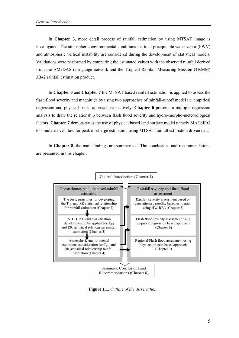
This dissertation comprises of 8 chapters which are outlined in Figure 1.1. In Chapter 1,
the background of the research is presented. In this chapter, the research objectives are also stated.
In Chapter 2, the basic approach and assumption of geostationary satellite based rainfall
estimation is introduced. Here the statistical relationship that is generated from collocated
MTSAT IR1 cloud top temperature (TIR1) and rainfall rate (RR) from TRMM 2A12 is applied and
validated. The study is conducted in Java Island Indonesia.
In Chapter 3, the cloud type classification is developed for supporting the assumption of
TIR1 and RR based rainfall estimation which is the method is suitable only for cumulonimbus (Cb)
cloud type. A new two-dimensional threshold diagram (2D-THR) has been developed based on
maximum likelihood cloud classification results, which can readily be applied for Multi-
functional Transport Satellite (MTSAT) split window datasets. The Cb cloud type derived from
the classification is used for improving TIR1 and RR based rainfall estimation.
In Chapter 4, the MTSAT based rainfall estimation by considering Cb cloud type is
applied to characterize the storm severity. The Hosking and Wallis regional frequency analysis
(HW-RFA) method is used to define the frequency distribution of long-term hourly maximum
rainfall over Hokkaido Island. Characterization of severity of 24 August 2010 storm event has
been performed over western part of Hokkaido Island, based on the regional frequency
distribution and the MTSAT rainfall estimation.
General Introduction
5
In Chapter 5, more detail process of rainfall estimation by using MTSAT image is
investigated. The atmospheric environmental conditions i.e. total precipitable water vapor (PWV)
and atmospheric vertical instability are considered during the development of statistical models.
Validations were performed by comparing the estimated values with the observed rainfall derived
from the AMeDAS rain gauge network and the Tropical Rainfall Measuring Mission (TRMM)
3B42 rainfall estimation product.
In Chapter 6 and Chapter 7 the MTSAT based rainfall estimation is applied to assess the
flash flood severity and magnitude by using two approaches of rainfall-runoff model i.e. empirical
regression and physical based approach respectively. Chapter 6 presents a multiple regression
analysis to draw the relationship between flash flood severity and hydro-morpho-meteorological
factors. Chapter 7 demonstrates the use of physical based land surface model namely MATSIRO
to simulate river flow for peak discharge estimation using MTSAT rainfall estimation driven data.
In Chapter 8, the main findings are summarized. The conclusions and recommendations
are presented in this chapter.
Figure 1.1. Outline of the dissertation.
General Introduction (Chapter 1)
Geostationary satellite based rainfall estimation
The basic principles for developing the TIR1 and RR statistical relationship
for rainfall estimation (Chapter 2)
2-D THR Cloud classification development to be applied for TIR1
and RR statistical relationship rainfall estimation (Chapter 3)
Atmospheric environmental conditions consideration for TIR1 and
RR statistical relationship rainfall estimation (Chapter 4)
Rainfall severity and flash flood assessment
Rainfall severity assessment based on geostationary satellite based estimation
using HW-RFA (Chapter 5)
Flash flood severity assessment using empirical regression based approach
(Chapter 6)
Regional Flash flood assessment using physical process based approach
(Chapter 7)
Summary, Conclusions and Recommendations (Chapter 8)
Chapter 2. GEOSTATIONARY SATELLITE BASED RAINFALL ESTIMATION AND VALIDATION
This chapter is based on: Suseno, Dwi Prabowo Yuga, T. J. Yamada, 2011, Geostationary Satellite Based
Rainfall Estimation and Validation: A Case Study of Java Island, Indonesia, Journal of Japan Society
of Civil Engineers, Ser. B1 (Hydraulic Engineering), Volume 67, Issue 4, pp. I_43-I_48
Geostationary satellite based rainfall estimation and validation
7
Abstract
Near real time rainfall information is necessary for early warning of rainfall triggered hazard such
as floods and landslides. Remote sensing based rainfall estimation has been considered to be used
to fulfill that purpose. This study is addressed to use geostationary based rainfall estimation by
using Multi Transport Satellite (MTSAT) data which is blended with Tropical Rainfall Measuring
Mission (TRMM) 2A12 datasets in order to provide near real time rainfall information, especially
for hazard study purposes over Java Island, Indonesia. The blending process is conducted by
developing statistical relationship between cloud top temperature from MTSAT 10.8µm channel
(TIR1) which is collocated with rainfall rate (RR) acquired by TRMM 2A12. Comparison to
TRMM Multi Precipitation Analysis (TMPA) datasets is performed. Spatial and temporal
validation of those rainfall estimations is conducted by validating them with available rain gauge
data during a rainy season in December 2007. Temporal validation result shows that TMPA
demonstrated better statistical performance than TIR1 and RR statistical relationship model.
However for the spatial correlation, TIR1 and RR statistical relationship model shows reasonably
better performance than TMPA.
Keywords: MTSAT, TRMM 2A12, TMPA, rainfall estimation, validation
Geostationary satellite based rainfall estimation and validation
8
2.1. INTRODUCTION
Floods and landslides are noticed as two of natural hazards that repeatedly occurred during
rainy seasons in Indonesia. Floods (e.g. inundation, flash flood, debris flow, etc) and landslide
that triggered by severe storm have very serious impact to the loss both infrastructures and lives.
As reported by SCTV (a private TV station in Indonesia) during December 2007, there were at
least 21 of big floods events in 8 landslides events struck several different places in Java Island
(SCTV 2008). Total casualties of the events for flood and landslide were 23 and 63 respectively
and the events cause losses of thousand houses and infrastructures.
Many of the natural hazard casualties can be avoided if there is an early warning to the
prone area due to the occurrence of successive high intensity of rainfall. The slow dissemination
of measured rainfall information most likely is considered as serious obstacle in terms of the use
of meteorological information for early warning purpose. It is because the limitation of
meteorological infrastructure itself. Many of them are still using manual measuring and recording
system instead of automatic measurement networks with telemetry system. Another drawback of
rain gauges measurement is that they are limited in spatial coverage.
A different system of rainfall measurement that nearly real-time, covers wide area and
depict spatial distribution of rainfall is necessary to implement. One of system that can be applied
is satellite based rainfall estimation data products. There are three methods that can use for
estimating rainfall from the satellite based upon type of observation i.e. (i) Visible and Infrared
(VIS/IR) method; (ii) Passive and Active Microwave Method (PMW); and (iii) Multisensor
Techniques Method (Kidd, et al., 2010). The VIS/IR method uses indirect approach for rainfall
estimation, i.e. according to top surface cloud characteristics such as shape, brightness,
temperature etc. Since the sensor is carried out by geostationary satellite, the global coverage of
rainfall estimation can be provided. The PMW method uses more direct rainfall estimation. It
utilizes interaction between hydrometeor and microwave such as scattering and emission. The
limitation of this method is that observations are currently only available from low earth orbit
satellite. It makes lower temporal resolution of PMW observation than VIS/IR method. The
mutisensor techniques combine the advantages of VIS/IR and PMW methods. The principle of
multisensor techniques is to adjust the IR using the other dataset such as radar, rain gauge or other
satellite datasets (Kidd, et al., 2010). There are several ready to use satellite rainfall estimation
products based on multisensor techniques such as TRMM Multi-satellite Precipitation Analysis
(TMPA), Climate Prediction Morphing Method (CMORPH), Precipitation Estimation from
Remotely Sensed Information using Artificial Neural Network Multispectral Analysis
(PERSIANN-MSA), and Global Satellite Mapping of Precipitation (GSMaP) (Kidd, et al., 2010).
Geostationary satellite based rainfall estimation and validation
9
The datasets are mainly delivered via internet through their respective dedicated product web page
location.
This study is addressed to perform rainfall estimation based on multisensor technique by
blending Multi-functional Transport Satellite (MTSAT) and Tropical Rainfall Measuring Mission
(TRMM) 2A12 dataset in order to provide near real time rainfall information, especially for
hazard study purposes. MTSAT that captured the hemisphere in a quite high temporal resolution
(1 hour) has good capability to monitor atmospheric condition such as rainfall by using its VIS/IR
sensors. However, cloud is opaque in VIS/IR spectral bands, so rainfall estimation by using those
of spectral bands are mainly based on the cloud top characteristics. In order to get more accurate
estimation, the advantage of TRMM is accommodated. TRMM has more direct rainfall estimation
due to its capability to penetrate the cloud and interact with hydrometeor.
Although there are several ready in use rainfall estimations freely available, the
development of rainfall estimation that uses fine resolution satellite such as geostationary satellite
dataset is still needed. The motivation of this study is to provide rainfall estimation for rainfall
triggered hazard such as flash flood. Most of flash flood events occurred in small river basin with
a drainage area of a few hundred square kilometers or less (NRC, 2005). Moreover flash flood is
triggered by very intense and short duration rainfall (Dingman, 2002). Some flash flood events
occurred in tropical regions such as Indonesia are triggered by isolated convective storm over
small river basin. The current available satellite-based rainfall datasets that mainly cover global
scale (i.e. 0.25° × 0.25° and 3 hours for TMPA) is considered relatively coarse resolution when it
is used for flash flood early warning detection purposes. Another consideration is due to the
indirect nature of the relationship between spectral information from satellite and corresponding
rainfall that makes those of rainfall prediction area not universally applicable (Wardah et al.,
2008).
There are two main objectives of this study. Firstly is to perform rainfall estimation based
on (TIR1) and RR statistical relationship. Secondly is to evaluate the performance of rainfall
estimation and to compare with ready to use rainfall estimation TMPA dataset by validating both
temporally and spatially with available rain gauge data.
2.2. THE STUDY AREA AND DATASETS
The study area is Java Island located on 5°S to 10°S and 95°E to 105°E (window size 5° × 10°).
For the validation purpose due to limitation of time of study and the availability of measured
Geostationary satellite based rainfall estimation and validation
10
rainfall data, only southern part of Central Java i.e. Yogyakarta city and its surrounding is selected.
The area of study and the validation area are presented in Figure 2.1.
The number of rainfall station situated in validation area is 22 automatic stations. Those of
rainfall stations are operated by several different institutions i.e.: SABO Agency (Balai SABO)
Yogyakarta, Public Work Agency of Progo Bogowonto Lukulo (Probolo Agency), Faculty of
Geography, Gadjah Mada University and Agricultural Technology Research Agency (Balai
Penelitian Teknologi Pertanian) of Yogyakarta.
The validation period is conducted during December 2007 (31 days). The rain gauge data is
mainly delivered in 1 hourly average rainfall, thus in this case there are 744 data. The same
number of MTSAT images is acquired from WebGMS-MTSAT/GMS (HIMAWARI) data
processing on WWW, Earthquake Research Institute & Institute of Industrial Science, University
of Tokyo. TMPA (also known as TRMM version 3B42) datasets are derived from
http://mirador.gsfc.nasa.gov.
2.3. METHOD AND VALIDATION SCHEMES
2.3.1. The blending process through TIR1 and RR statistical relationship
The method that is used in the current study mainly is adopted from the algorithm
developed by Maathuis (Maathuis et al., 2006). The method has been chosen because it is
relatively simple both in data need and process, affordable for non-meteorologist and low cost
computing. The original method uses Meteosat Second Generation (MSG) and TRMM as data
input. Since this study is conducted over Java Island that isn’t covered by MSG, therefore
MTSAT and TRMM are utilized as data input. Here, it assumed that the IR band (10.8 µm) of
MSG is comparable to IR1 (10.3µm – 11.3µm) of MTSAT and the water vapor band (6.2µm) of
MSG is comparable to IR3 (6.5µm – 7 µm) of MTSAT.
(b)
(a)
Figure 2.1. (a) Study area which cover Java Island and (b) validation area that cover Yogyakarta
and its surrounding area.
Geostationary satellite based rainfall estimation and validation
11
The basic idea of TIR1 and RR based rainfall estimation is to develop statistical relationship
between cloud top temperature depicted by MTSAT IR1 datasets (TIR1) and rain rate observed by
TRMM 2A12 datasets (RR). For the convective cloud situation, the relationship between cloud
top temperature and rain rate shows that the low cloud top temperature is associated with heavier
rainfall (Kuligowski, 2003). A statistical regression should be developed to express that
relationship. To draw such statistical relationship the exponential curve is used. It means that the
rain rate is decreasing exponentially along the increasing of cloud top brightness temperature
(Vicente et al., 1998). The developed statistical regression will be used to generate rainfall
estimation based on MTSAT datasets.
The most important step during performing this method is how to get collocated image both
temporally and spatially between MTSAT and TRMM dataset. It is a prerequisite in order to
develop strong statistical relationship between cloud top temperature and rainfall rate. The ideal
collocated image is those of MTSAT data and TRMM data that have the same acquisition time
over the same area. In the real situation this ideal condition is difficult to fulfill. Actually, only the
collocated images that have almost the same time of acquisition over the area can be selected.
Because of the lag of acquisition time, a slightly discrepancy of cloud spatial distribution is
depicted in collocated image.
In order to reduce such discrepancy, an averaging process for TRMM data based on the
grouped MTSAT-IR cloud temperature (e.g. 0.5 K or 1 K equal range temperature) is performed
(Maathuis et al., 2006). This process can increase the correlation coefficient of the relationship
between cloud top temperature and rainfall rate. The discrepancy is tried to be reduced by limiting
the coverage of collocated image during statistical relationship development. This process is
performed to improve the original algorithm that used whole coverage as collocation window.
The collocated window size that used by Heinemann et al. (2008) i.e. 5º × 5º to divide the whole
domain window size into two smaller windows has been adopted. The relationship of both
windows is examined by comparing the correlation coefficient. The best statistical relationship is
chosen to estimate the rainfall of whole coverage area.
The last process for rainfall data generation is performed by the best regression equation
based on MTSAT cloud temperature. The rainfall data generation process is only applied to the
MTSAT cloud top temperature that considered as potential precipitating cloud. The potential
precipitating cloud has been selected by the brightness temperature difference between IR1 and
IR3 that is less than 11 K (Maathuis et al., 2006). Each regression function will valid to certain
range of MTSAT image series. Figure 2.2 shows the schematic diagram of rainfall estimation
using TIR1 and RR statistical relationship used in this study.
Geostationary satellite based rainfall estimation and validation
12
Figure 2.2. Blending method between TIR1 and RR derived from MTSAT and TRMM 2A12
respectively.
2.3.2. Validation Schemes and Statistical Analysis
In order to measure the performance of TIR1 and RR based rainfall estimation, a validation is
performed by comparing it with rain gauge data both in temporally and spatially scales. As a
comparison, the same validation process is also performed for the TMPA datasets.
Temporal validation is performed in point to pixel basis i.e. point rainfall data from rain
gauge measurement and pixel based rainfall estimation from satellite. Hourly average and 3
hourly average rain gauge data are used to validate TIR1 and RR based rainfall estimation and
TMPA rainfall estimation respectively. Pixel information that contains rainfall estimation from
satellite is retrieved according to the coordinate location of rainfall stations. For each rain gauge
location, a pair of estimated and observed rainfall has been generated.
Statistical comparison has been performed for those of pair data. Some categorical statistics
has been employed such as accuracy, bias score, Probability of Detection (POD), False Alarm
Geostationary satellite based rainfall estimation and validation
13
Ratio (FAR) and Critical Success Index (CSI) to evaluate the performance of rainfall estimation
from satellites.
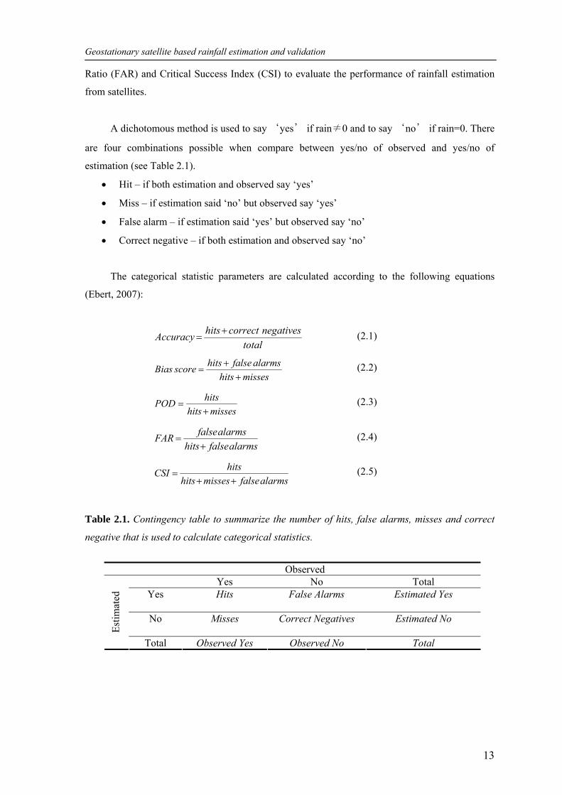
A dichotomous method is used to say ‘yes’ if rain≠0 and to say ‘no’ if rain=0. There
are four combinations possible when compare between yes/no of observed and yes/no of
estimation (see Table 2.1).
• Hit – if both estimation and observed say ‘yes’
• Miss – if estimation said ‘no’ but observed say ‘yes’
• False alarm – if estimation said ‘yes’ but observed say ‘no’
• Correct negative – if both estimation and observed say ‘no’
The categorical statistic parameters are calculated according to the following equations
(Ebert, 2007):
totalnegativescorrecthitsAccuracy +
= (2.1)
misseshitsalarmsfalsehitsscoreBias
++
= (2.2)
misseshitshitsPOD+
= (2.3)
alarmsfalsehitsalarmsfalseFAR
+= (2.4)
alarmsfalsemisseshitshitsCSI++
= (2.5)
Table 2.1. Contingency table to summarize the number of hits, false alarms, misses and correct
negative that is used to calculate categorical statistics.
Observed
Yes No Total Yes Hits
False Alarms Estimated Yes
No Misses
Correct Negatives Estimated No
Estim
ated
Total Observed Yes Observed No Total
Geostationary satellite based rainfall estimation and validation
14
Spatial validation is performed by calculating spatial correlation both in pixel to point and
pixel to pixel basis. Spatial correlation is defined as the correlation between estimated and
observed rainfall with respect to their geographical locations. In this study the spatial correlation
is investigated only for convective rainfall cases. For pixel to point validation, the spatial
correlation between rainfall estimation from satellite and corresponding measured rainfall data is
calculated. In terms of pixel to point validation there is a remaining problem which is related to
the type of data itself. Rainfall observation is considered as point data type otherwise satellite
based precipitation is area data type (measured as pixel area) (Grimes et al., 1999). In order to
make comparable validation, a pixel to pixel based spatial correlation is conducted. It means that
the pixel from satellite rainfall estimation is compared with the pixel (grid) of interpolated
observed rainfall which has the same geo-reference. The interpolated observed rainfall is
generated by using the block kriging interpolation method.
2.4. RESULTS AND DISCUSSIONS
2.4.1. Temporal validation
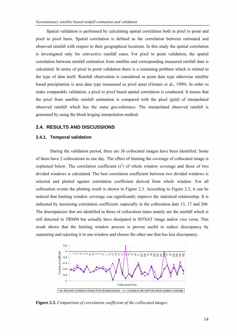
During the validation period, there are 36 collocated images have been identified. Some
of them have 2 collocations in one day. The effect of limiting the coverage of collocated image is
explained below. The correlation coefficient (r2) of whole window coverage and those of two
divided windows is calculated. The best correlation coefficient between two divided windows is
selected and plotted against correlation coefficient derived from whole window. For all
collocation events the plotting result is shown in Figure 2.3. According to Figure 2.3, it can be
noticed that limiting window coverage can significantly improve the statistical relationship. It is
indicated by increasing correlation coefficient, especially in the collocation date 13, 17 and 26b.
The discrepancies that are identified in those of collocation times mainly are the rainfall which is
still detected in TRMM but actually have dissipated in MTSAT image and/or vice versa. This
result shows that the limiting window process is proven useful to reduce discrepancy by
separating and rejecting it in one window and choose the other one that has less discrepancy.
Figure 2.3. Comparison of correlation coefficient of the collocated images.
Geostationary satellite based rainfall estimation and validation
15
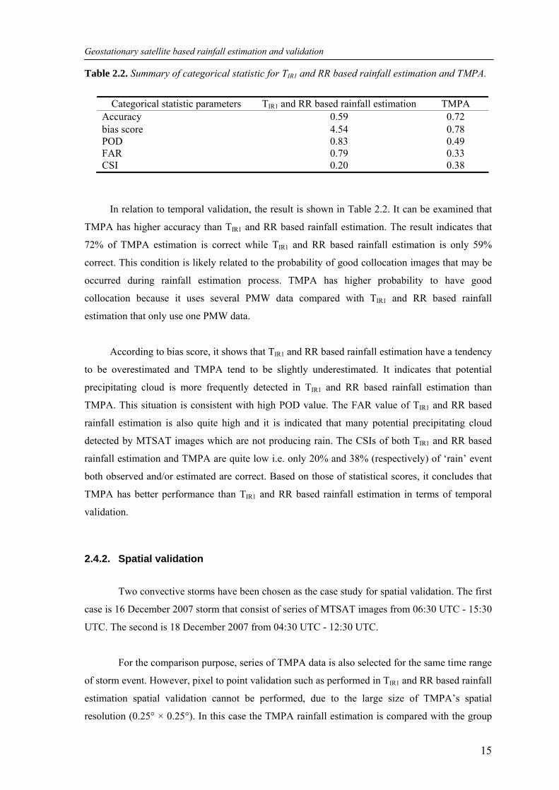
Table 2.2. Summary of categorical statistic for TIR1 and RR based rainfall estimation and TMPA.
Categorical statistic parameters TIR1 and RR based rainfall estimation TMPA
Accuracy 0.59 0.72 bias score 4.54 0.78 POD 0.83 0.49 FAR 0.79 0.33 CSI 0.20 0.38
In relation to temporal validation, the result is shown in Table 2.2. It can be examined that
TMPA has higher accuracy than TIR1 and RR based rainfall estimation. The result indicates that
72% of TMPA estimation is correct while TIR1 and RR based rainfall estimation is only 59%
correct. This condition is likely related to the probability of good collocation images that may be
occurred during rainfall estimation process. TMPA has higher probability to have good
collocation because it uses several PMW data compared with TIR1 and RR based rainfall
estimation that only use one PMW data.
According to bias score, it shows that TIR1 and RR based rainfall estimation have a tendency
to be overestimated and TMPA tend to be slightly underestimated. It indicates that potential
precipitating cloud is more frequently detected in TIR1 and RR based rainfall estimation than
TMPA. This situation is consistent with high POD value. The FAR value of TIR1 and RR based
rainfall estimation is also quite high and it is indicated that many potential precipitating cloud
detected by MTSAT images which are not producing rain. The CSIs of both TIR1 and RR based
rainfall estimation and TMPA are quite low i.e. only 20% and 38% (respectively) of ‘rain’ event
both observed and/or estimated are correct. Based on those of statistical scores, it concludes that
TMPA has better performance than TIR1 and RR based rainfall estimation in terms of temporal
validation.
2.4.2. Spatial validation
Two convective storms have been chosen as the case study for spatial validation. The first
case is 16 December 2007 storm that consist of series of MTSAT images from 06:30 UTC - 15:30
UTC. The second is 18 December 2007 from 04:30 UTC - 12:30 UTC.
For the comparison purpose, series of TMPA data is also selected for the same time range
of storm event. However, pixel to point validation such as performed in TIR1 and RR based rainfall
estimation spatial validation cannot be performed, due to the large size of TMPA’s spatial
resolution (0.25° × 0.25°). In this case the TMPA rainfall estimation is compared with the group
Geostationary satellite based rainfall estimation and validation
16
of rainfall station as average observation rather than individual station. The group of rainfall
stations is defined according to the spatial resolution of TMPA. The centroid of corresponding
TMPA’s pixel has been considered as coordinate location of each group. Spatial correlation is
calculated based on those average rainfall observation from group of stations and TMPA rainfall
estimation, in the same coordinate location.
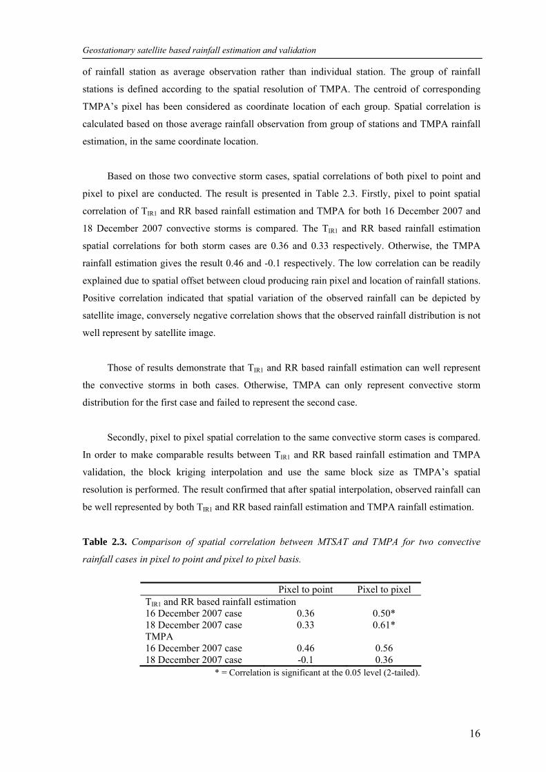
Based on those two convective storm cases, spatial correlations of both pixel to point and
pixel to pixel are conducted. The result is presented in Table 2.3. Firstly, pixel to point spatial
correlation of TIR1 and RR based rainfall estimation and TMPA for both 16 December 2007 and
18 December 2007 convective storms is compared. The TIR1 and RR based rainfall estimation
spatial correlations for both storm cases are 0.36 and 0.33 respectively. Otherwise, the TMPA
rainfall estimation gives the result 0.46 and -0.1 respectively. The low correlation can be readily
explained due to spatial offset between cloud producing rain pixel and location of rainfall stations.
Positive correlation indicated that spatial variation of the observed rainfall can be depicted by
satellite image, conversely negative correlation shows that the observed rainfall distribution is not
well represent by satellite image.
Those of results demonstrate that TIR1 and RR based rainfall estimation can well represent
the convective storms in both cases. Otherwise, TMPA can only represent convective storm
distribution for the first case and failed to represent the second case.
Secondly, pixel to pixel spatial correlation to the same convective storm cases is compared.
In order to make comparable results between TIR1 and RR based rainfall estimation and TMPA
validation, the block kriging interpolation and use the same block size as TMPA’s spatial
resolution is performed. The result confirmed that after spatial interpolation, observed rainfall can
be well represented by both TIR1 and RR based rainfall estimation and TMPA rainfall estimation.
Table 2.3. Comparison of spatial correlation between MTSAT and TMPA for two convective
rainfall cases in pixel to point and pixel to pixel basis.
Pixel to point Pixel to pixel TIR1 and RR based rainfall estimation 16 December 2007 case 0.36 0.50* 18 December 2007 case 0.33 0.61* TMPA 16 December 2007 case 0.46 0.56 18 December 2007 case -0.1 0.36
* = Correlation is significant at the 0.05 level (2-tailed).
Geostationary satellite based rainfall estimation and validation
17
The average of spatial correlation of TIR1 and RR based rainfall estimation and TMPA from both
two cases is calculated. The calculation results are 0.56 and 0.46 for TIR1 and RR based rainfall
estimation and TMPA respectively. It shows that in average TIR1 and RR based rainfall estimation
demonstrates better spatial representation of convective rainfall than TMPA.
The average value of spatial correlation of MTSAT (i.e. 0.56) has good agreement with the
result of Ebert and Manton’s study (Ebert and Manton, 1998) that for the instantaneous rainfall of
mixed geostationary satellite and polar orbit satellite (IR-SSM/I) algorithms has correlation
coefficient ranging from 0.49 to 0.55.
2.5. SUMMARY AND CONCLUSIONS
Regarding to the temporal validation, TMPA shows relatively better performance than TIR1
and RR based rainfall estimation. It could be explained mainly because of TMPA algorithm
developed based on various data inputs as well as complex algorithm. The relatively low
statistical performance of TIR1 and RR based rainfall estimation rainfall estimation compared to
TMPA is considered as the limitation of this method. It might be because of the overestimate of
potential precipitating cloud detected by TIR1 and RR based rainfall estimation. For the further
study, the more accurately potential precipitating cloud detection should be adopted. Furthermore,
limiting collocated window method that already shows a promising result should be enhanced.
However for the spatial correlation, TIR1 and RR based rainfall estimation is demonstrated
better performance than TMPA. With regards to this potentiality, TIR1 and RR based rainfall
estimation algorithm is quite promising as an alternative method for providing rainfall data for
ungauged remote area. It can be used also as an indirect approach for the rainfall triggered hazard
early warning system. It is because TIR1 and RR based rainfall estimation has shown quite good to
represent spatial distribution of rainfall especially convective storm events, though the accuracy of
rainfall detection should be increased. The convective storm is characterized by very intense rain
in short duration (lasting less than 1 hour) and covers small area (Dingman, 2002). This type of
rainfall has been considered as the causing factor of flash flood (Wardah et al., 2008). Based on
this relation, MTSAT dataset that have good spatial and temporal resolution can be considered to
be used for such kind of rainfall related hazard studies. Another consideration is that TIR1 and RR
based rainfall estimation is only need simple data input and processing and low cost computing.
This consideration is beneficial in term of practical point of view.
Chapter 3. REMOTE SENSING BASED CLOUD TYPE CLASSIFICATION FOR SUPPORTING RAINFALL ESTIMATION
This chapter is based on:
Suseno, Dwi Prabowo Yuga, T. J. Yamada, 2011, The Use of Cloud Type Classification To Improve
Geostationary Based Rainfall Estimation. 9th International Symposium on Southeast Asian Water
Environment, Dec 1st-3rd 2011 Bangkok City, Thailand.
Suseno, Dwi Prabowo Yuga, T. J. Yamada, 2012, Two-dimensional threshold-based cloud-type
classification using MTSAT data, Remote Sensing Letters, Vol. 3 Issue 8. pp 737-746.
Remote Sensing Based Cloud Type Classification For Supporting Rainfall Estimation
19
Abstract
A new two-dimensional threshold diagram (2D-THR) has been developed based on
maximum likelihood cloud classification results, which can readily be applied for Multi-
functional Transport Satellite (MTSAT) split window datasets. Since 2D-THR was trained using
northern summer 2010 data for Japan and its surrounding area, it is typically suitable only for
summer. Comparison of snapshot cloud-type distributions showed that 2D-THR images and the
corresponding night-time microphysical colour composite images as well as 2D-THR and Japan
Meteorological Agency (JMA) cloud-type images are in good agreement. A time series inter-
comparison of the hourly 2D-THR cloud classification results with the JMA cloud type
classification data product was performed by calculating spatial correlation of cloud percentage
for 1° × 1° grid cells. For cumulonimbus, high-level, middle-level, and low-level clouds over
tropical and subtropical areas in the northwestern Pacific Ocean region, the spatial correlation
between 2D-THR and JMA is moderate. Thus, 2D-THR cloud-classification algorithm can be
applied in both regions. Integrating the cloud type classification especially by separating
Cumulonimbus (Cb) cloud type from other cloud types can improve the MTSAT 10.8µm cloud
top temperature (TIR1) and rainfall rate (RR) relationship, which is indicated by increasing
correlation coefficient and the gradient of regression line. Moreover, underestimating rainfall
intensity can be avoided by applying rainfall rate and cloud top temperature relationship that uses
Cb cloud type only rather than using all cloud types. A good agreement between estimated and
measured storm rainfall also has been demonstrated when use this approach.
Keywords: Cloud type classification, MTSAT, 2D threshold diagram, rainfall estimation
Remote Sensing Based Cloud Type Classification For Supporting Rainfall Estimation
20
3.1. INTRODUCTION
In an early warning system of rainfall triggered hazard such as flood and landslide, storm
rainfall data is key information. Storm rainfall data should be prepared as soon as possible in
order to provide sufficient warning time. The use of measured rainfall data for early warning
purpose sometimes is not enough because the rainfall event actually had been occurred so
available times for warning become limited. The other problem is the distribution of the rain
gauge sometimes too sparse, even ungauged in some remote places. In this regards the use remote
sensing technology for rainfall estimation is a practical alternative to be applied to overcome
those of problems.
One approach of using remote sensing for rainfall estimation is multisensor approach i.e. by
developing the relationship between cloud properties data provided by satellite sensors and
rainfall data measured by gauge or other satellite sensors in the same collocated time and space. A
rainfall estimation study based on relationship between rainfall rate and satellite based cloud top
brightness temperature and rainfall rate relationship (TBB and RR relationship hereinafter) had
been conducted by employing MTSAT and Tropical Rainfall Measuring Mission (TRMM)
datasets over Java Island, Indonesia (Suseno and Yamada, 2011a). The cloud top temperature is
related to rainfall rate which lower cloud top temperature is associated with heavier rainfall.
However this assumption is reasonable for convective cloud type such as Cumulonimbus (Cb) but
poor for other cloud type such as Cirrus (Ci) that cold but light or no rain and stratiform clouds
that warm but wet (Kuligowski, 2003). In order to fulfill this assumption cloud type information
is necessary to be integrated in the multisensor rainfall estimation approach.
On the subject of cloud classification, there are several satellites and methods have been
used and developed as well. The cloud type classification method generally can be categorized as
supervised classification and unsupervised classification. Supervised classification uses specific
areas in the satellite image that defined by analyst which represents homogenous example of earth
object. These areas are commonly referred to as training sites because the spectral characteristics
of these known areas are used to train the classification algorithm for eventual earth objects
mapping of the remainder of the remote sensing image (Jensen, 2005). The benefit of using
supervised classification is that analyst can control the categories or classes according their
specific purpose. However this method is time consuming, especially during training area
selection. On the purpose of early warning which speed processing time is necessary, this method
is not practical. The unsupervised classification which uses simple process such as thresholding
technique is more common to be used (Inoue, 1987; Lensky et al., 2003; Saunders, 1988).
Threshold classification uses a specific or a range of spectral values as the boundary among the
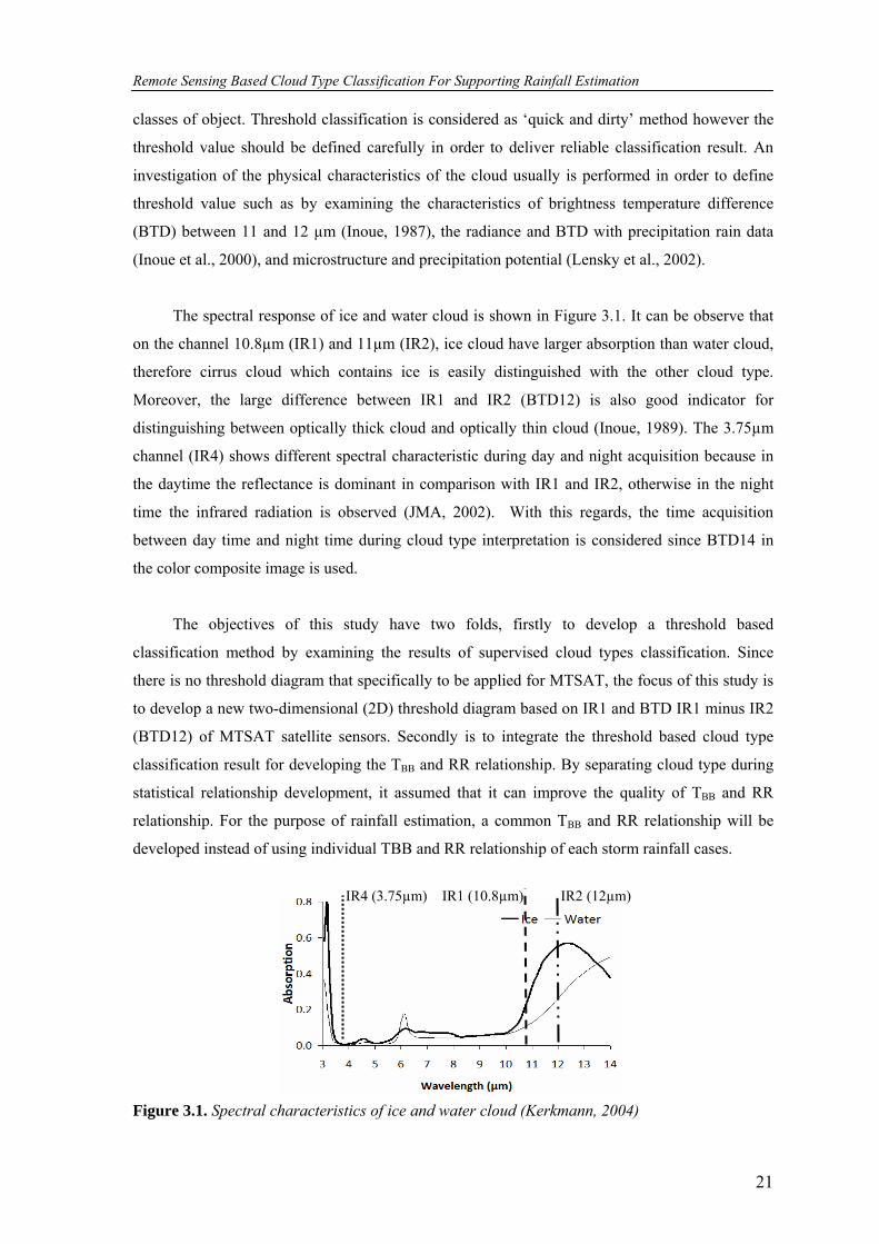
Remote Sensing Based Cloud Type Classification For Supporting Rainfall Estimation
21
classes of object. Threshold classification is considered as ‘quick and dirty’ method however the
threshold value should be defined carefully in order to deliver reliable classification result. An
investigation of the physical characteristics of the cloud usually is performed in order to define
threshold value such as by examining the characteristics of brightness temperature difference
(BTD) between 11 and 12 µm (Inoue, 1987), the radiance and BTD with precipitation rain data
(Inoue et al., 2000), and microstructure and precipitation potential (Lensky et al., 2002).
The spectral response of ice and water cloud is shown in Figure 3.1. It can be observe that
on the channel 10.8µm (IR1) and 11µm (IR2), ice cloud have larger absorption than water cloud,
therefore cirrus cloud which contains ice is easily distinguished with the other cloud type.
Moreover, the large difference between IR1 and IR2 (BTD12) is also good indicator for
distinguishing between optically thick cloud and optically thin cloud (Inoue, 1989). The 3.75µm
channel (IR4) shows different spectral characteristic during day and night acquisition because in
the daytime the reflectance is dominant in comparison with IR1 and IR2, otherwise in the night
time the infrared radiation is observed (JMA, 2002). With this regards, the time acquisition
between day time and night time during cloud type interpretation is considered since BTD14 in
the color composite image is used.
The objectives of this study have two folds, firstly to develop a threshold based
classification method by examining the results of supervised cloud types classification. Since
there is no threshold diagram that specifically to be applied for MTSAT, the focus of this study is
to develop a new two-dimensional (2D) threshold diagram based on IR1 and BTD IR1 minus IR2
(BTD12) of MTSAT satellite sensors. Secondly is to integrate the threshold based cloud type
classification result for developing the TBB and RR relationship. By separating cloud type during
statistical relationship development, it assumed that it can improve the quality of TBB and RR
relationship. For the purpose of rainfall estimation, a common TBB and RR relationship will be
developed instead of using individual TBB and RR relationship of each storm rainfall cases.
IR4 (3.75µm) IR1 (10.8µm) IR2 (12µm)
Figure 3.1. Spectral characteristics of ice and water cloud (Kerkmann, 2004)
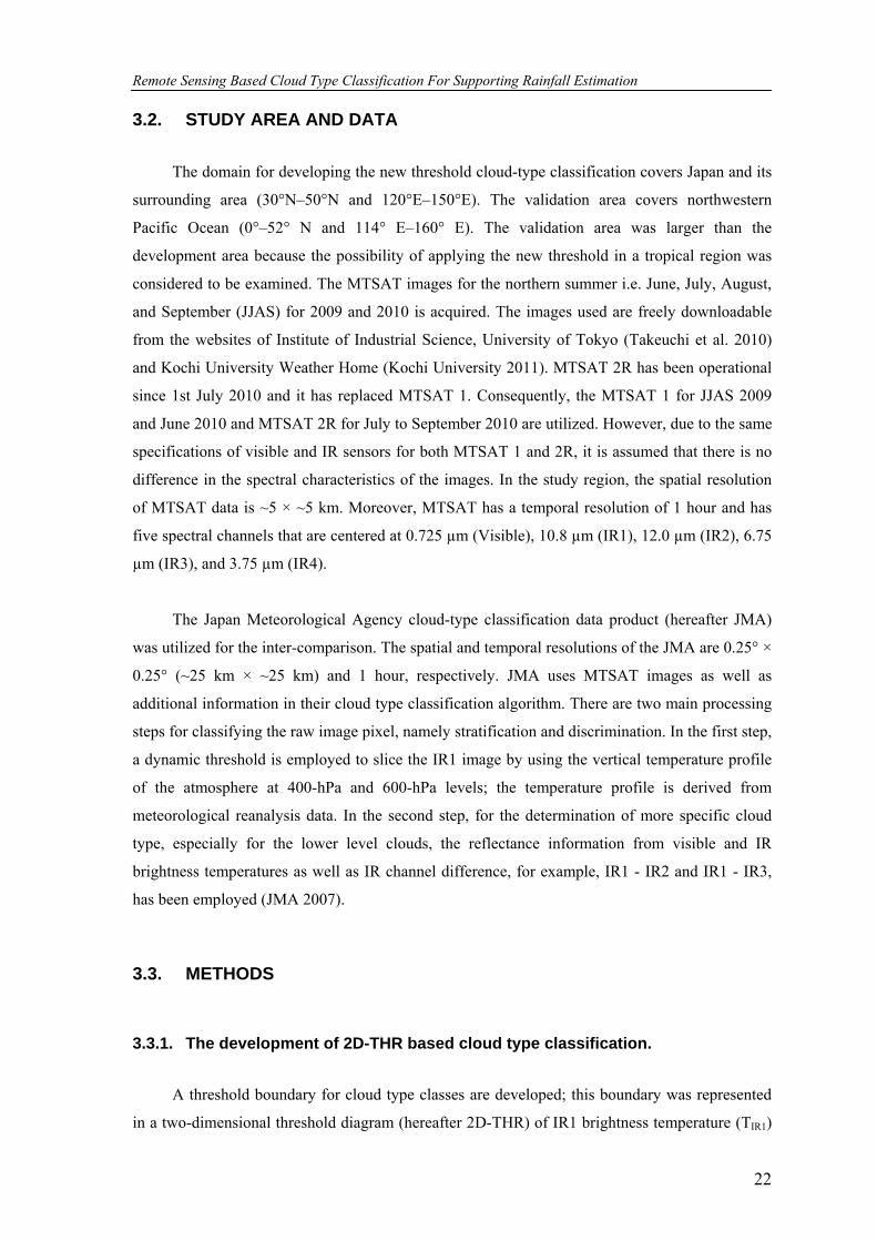
Remote Sensing Based Cloud Type Classification For Supporting Rainfall Estimation
22
3.2. STUDY AREA AND DATA
The domain for developing the new threshold cloud-type classification covers Japan and its
surrounding area (30°N–50°N and 120°E–150°E). The validation area covers northwestern
Pacific Ocean (0°–52° N and 114° E–160° E). The validation area was larger than the
development area because the possibility of applying the new threshold in a tropical region was
considered to be examined. The MTSAT images for the northern summer i.e. June, July, August,
and September (JJAS) for 2009 and 2010 is acquired. The images used are freely downloadable
from the websites of Institute of Industrial Science, University of Tokyo (Takeuchi et al. 2010)
and Kochi University Weather Home (Kochi University 2011). MTSAT 2R has been operational
since 1st July 2010 and it has replaced MTSAT 1. Consequently, the MTSAT 1 for JJAS 2009
and June 2010 and MTSAT 2R for July to September 2010 are utilized. However, due to the same
specifications of visible and IR sensors for both MTSAT 1 and 2R, it is assumed that there is no
difference in the spectral characteristics of the images. In the study region, the spatial resolution
of MTSAT data is ~5 × ~5 km. Moreover, MTSAT has a temporal resolution of 1 hour and has
five spectral channels that are centered at 0.725 µm (Visible), 10.8 µm (IR1), 12.0 µm (IR2), 6.75
µm (IR3), and 3.75 µm (IR4).
The Japan Meteorological Agency cloud-type classification data product (hereafter JMA)
was utilized for the inter-comparison. The spatial and temporal resolutions of the JMA are 0.25° ×
0.25° (~25 km × ~25 km) and 1 hour, respectively. JMA uses MTSAT images as well as
additional information in their cloud type classification algorithm. There are two main processing
steps for classifying the raw image pixel, namely stratification and discrimination. In the first step,
a dynamic threshold is employed to slice the IR1 image by using the vertical temperature profile
of the atmosphere at 400-hPa and 600-hPa levels; the temperature profile is derived from
meteorological reanalysis data. In the second step, for the determination of more specific cloud
type, especially for the lower level clouds, the reflectance information from visible and IR
brightness temperatures as well as IR channel difference, for example, IR1 - IR2 and IR1 - IR3,
has been employed (JMA 2007).
3.3. METHODS
3.3.1. The development of 2D-THR based cloud type classification.
A threshold boundary for cloud type classes are developed; this boundary was represented
in a two-dimensional threshold diagram (hereafter 2D-THR) of IR1 brightness temperature (TIR1)
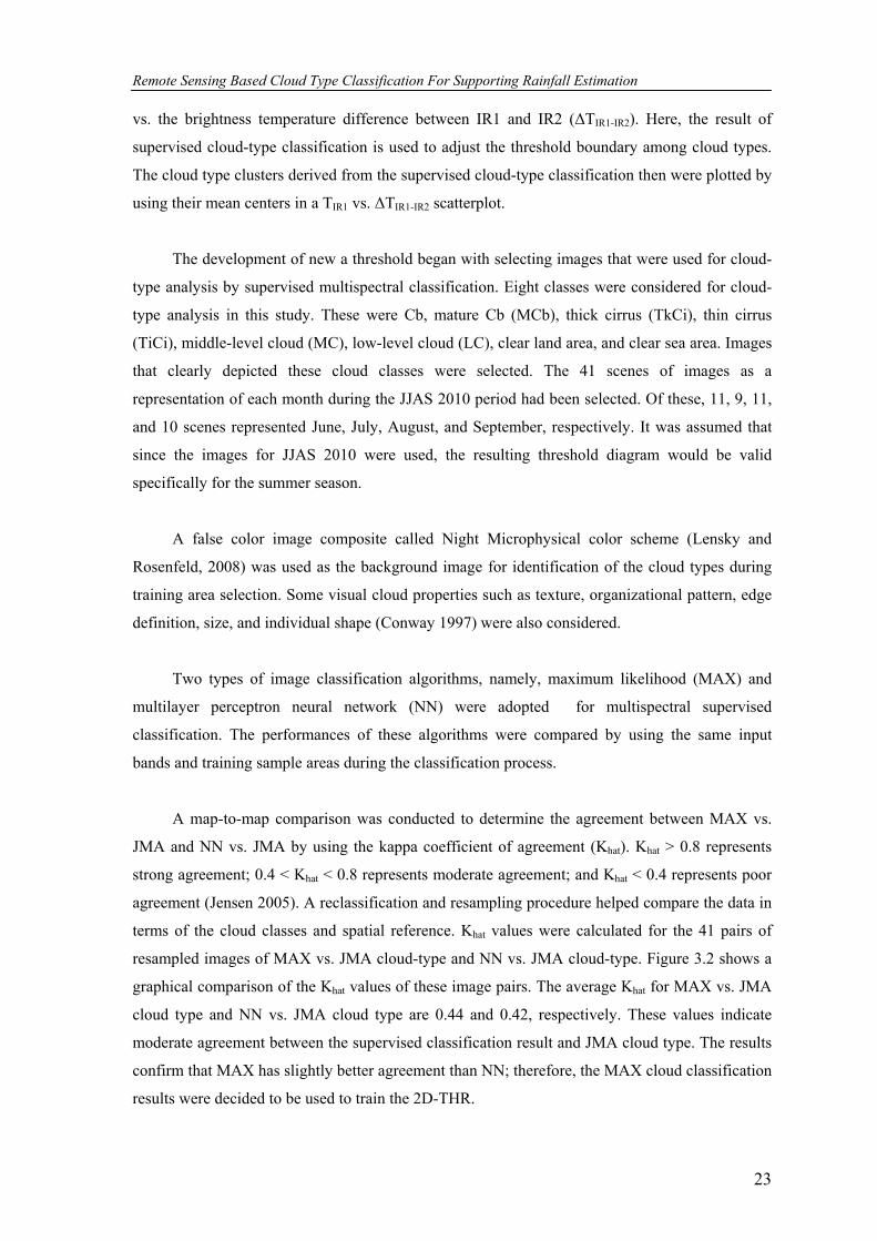
Remote Sensing Based Cloud Type Classification For Supporting Rainfall Estimation
23
vs. the brightness temperature difference between IR1 and IR2 (ΔTIR1-IR2). Here, the result of
supervised cloud-type classification is used to adjust the threshold boundary among cloud types.
The cloud type clusters derived from the supervised cloud-type classification then were plotted by
using their mean centers in a TIR1 vs. ΔTIR1-IR2 scatterplot.
The development of new a threshold began with selecting images that were used for cloud-
type analysis by supervised multispectral classification. Eight classes were considered for cloud-
type analysis in this study. These were Cb, mature Cb (MCb), thick cirrus (TkCi), thin cirrus
(TiCi), middle-level cloud (MC), low-level cloud (LC), clear land area, and clear sea area. Images
that clearly depicted these cloud classes were selected. The 41 scenes of images as a
representation of each month during the JJAS 2010 period had been selected. Of these, 11, 9, 11,
and 10 scenes represented June, July, August, and September, respectively. It was assumed that
since the images for JJAS 2010 were used, the resulting threshold diagram would be valid
specifically for the summer season.
A false color image composite called Night Microphysical color scheme (Lensky and
Rosenfeld, 2008) was used as the background image for identification of the cloud types during
training area selection. Some visual cloud properties such as texture, organizational pattern, edge
definition, size, and individual shape (Conway 1997) were also considered.
Two types of image classification algorithms, namely, maximum likelihood (MAX) and
multilayer perceptron neural network (NN) were adopted for multispectral supervised
classification. The performances of these algorithms were compared by using the same input
bands and training sample areas during the classification process.
A map-to-map comparison was conducted to determine the agreement between MAX vs.
JMA and NN vs. JMA by using the kappa coefficient of agreement (Khat). Khat > 0.8 represents
strong agreement; 0.4 < Khat < 0.8 represents moderate agreement; and Khat < 0.4 represents poor
agreement (Jensen 2005). A reclassification and resampling procedure helped compare the data in
terms of the cloud classes and spatial reference. Khat values were calculated for the 41 pairs of
resampled images of MAX vs. JMA cloud-type and NN vs. JMA cloud-type. Figure 3.2 shows a
graphical comparison of the Khat values of these image pairs. The average Khat for MAX vs. JMA
cloud type and NN vs. JMA cloud type are 0.44 and 0.42, respectively. These values indicate
moderate agreement between the supervised classification result and JMA cloud type. The results
confirm that MAX has slightly better agreement than NN; therefore, the MAX cloud classification
results were decided to be used to train the 2D-THR.
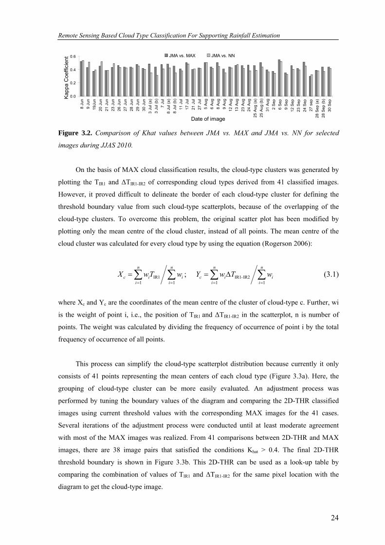
Remote Sensing Based Cloud Type Classification For Supporting Rainfall Estimation
24
0.0
0.2
0.4
0.6
8 Ju
n9
Jun
19Ju
n20
Jun
21 J
un23
Jun
26 J
un27
Jun
28 J
un29
Jun
30 J
un3
Jul (
a)3
Jul (
b)7
Jul
8 Ju
l (a)
8 Ju
l (b)
11 J
ul17
Jul
21 J
ul27
Jul
5 A
ug6
Aug
8 A
ug9
Aug
12 A
ug13
Aug
23 A
ug24
Aug
25 A
ug (a
)25
Aug
(b)
31 A
ug2
Sep
6 S
ep9
Sep
12 S
ep23
Sep
24 S
ep27
sep
28 S
ep (a
)28
Sep
(b)
30 S
ep
Date of image
Kapp
a C
oeffi
cien
t JMA vs. MAX JMA vs. NN
Figure 3.2. Comparison of Khat values between JMA vs. MAX and JMA vs. NN for selected
images during JJAS 2010.
On the basis of MAX cloud classification results, the cloud-type clusters was generated by
plotting the TIR1 and ΔTIR1-IR2 of corresponding cloud types derived from 41 classified images.
However, it proved difficult to delineate the border of each cloud-type cluster for defining the
threshold boundary value from such cloud-type scatterplots, because of the overlapping of the
cloud-type clusters. To overcome this problem, the original scatter plot has been modified by
plotting only the mean centre of the cloud cluster, instead of all points. The mean centre of the
cloud cluster was calculated for every cloud type by using the equation (Rogerson 2006):
∑∑∑∑====
Δ==n
ii
n
iic
n
ii
n
iic wTwYwTwX
11IR2-IR1
11IR1 ; (3.1)
where Xc and Yc are the coordinates of the mean centre of the cluster of cloud-type c. Further, wi
is the weight of point i, i.e., the position of TIR1 and ΔTIR1-IR2 in the scatterplot, n is number of
points. The weight was calculated by dividing the frequency of occurrence of point i by the total
frequency of occurrence of all points.
This process can simplify the cloud-type scatterplot distribution because currently it only
consists of 41 points representing the mean centers of each cloud type (Figure 3.3a). Here, the
grouping of cloud-type cluster can be more easily evaluated. An adjustment process was
performed by tuning the boundary values of the diagram and comparing the 2D-THR classified
images using current threshold values with the corresponding MAX images for the 41 cases.
Several iterations of the adjustment process were conducted until at least moderate agreement
with most of the MAX images was realized. From 41 comparisons between 2D-THR and MAX
images, there are 38 image pairs that satisfied the conditions Khat > 0.4. The final 2D-THR
threshold boundary is shown in Figure 3.3b. This 2D-THR can be used as a look-up table by
comparing the combination of values of TIR1 and ΔTIR1-IR2 for the same pixel location with the
diagram to get the cloud-type image.
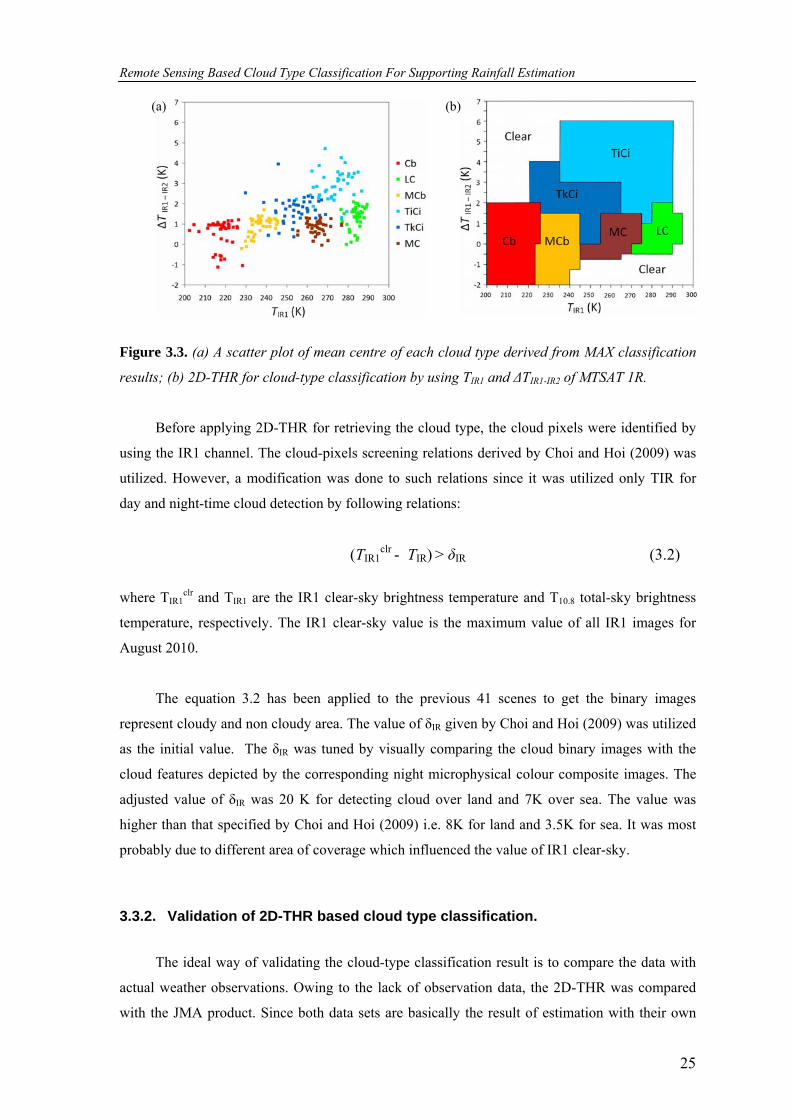
Remote Sensing Based Cloud Type Classification For Supporting Rainfall Estimation
25
(a) (b)
Figure 3.3. (a) A scatter plot of mean centre of each cloud type derived from MAX classification
results; (b) 2D-THR for cloud-type classification by using TIR1 and ΔTIR1-IR2 of MTSAT 1R.
Before applying 2D-THR for retrieving the cloud type, the cloud pixels were identified by
using the IR1 channel. The cloud-pixels screening relations derived by Choi and Hoi (2009) was
utilized. However, a modification was done to such relations since it was utilized only TIR for
day and night-time cloud detection by following relations:
(TIR1clr - TIR) > δIR (3.2)
where TIR1clr and TIR1 are the IR1 clear-sky brightness temperature and T10.8 total-sky brightness
temperature, respectively. The IR1 clear-sky value is the maximum value of all IR1 images for
August 2010.
The equation 3.2 has been applied to the previous 41 scenes to get the binary images
represent cloudy and non cloudy area. The value of δIR given by Choi and Hoi (2009) was utilized
as the initial value. The δIR was tuned by visually comparing the cloud binary images with the
cloud features depicted by the corresponding night microphysical colour composite images. The
adjusted value of δIR was 20 K for detecting cloud over land and 7K over sea. The value was
higher than that specified by Choi and Hoi (2009) i.e. 8K for land and 3.5K for sea. It was most
probably due to different area of coverage which influenced the value of IR1 clear-sky.
3.3.2. Validation of 2D-THR based cloud type classification.
The ideal way of validating the cloud-type classification result is to compare the data with
actual weather observations. Owing to the lack of observation data, the 2D-THR was compared
with the JMA product. Since both data sets are basically the result of estimation with their own
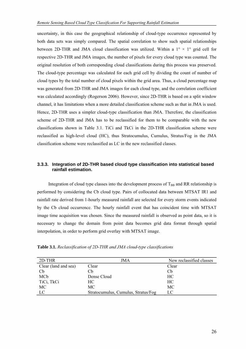
Remote Sensing Based Cloud Type Classification For Supporting Rainfall Estimation
26
uncertainty, in this case the geographical relationship of cloud-type occurrence represented by
both data sets was simply compared. The spatial correlation to show such spatial relationships
between 2D-THR and JMA cloud classification was utilized. Within a 1° × 1° grid cell for
respective 2D-THR and JMA images, the number of pixels for every cloud type was counted. The
original resolution of both corresponding cloud classifications during this process was preserved.
The cloud-type percentage was calculated for each grid cell by dividing the count of number of
cloud types by the total number of cloud pixels within the grid area. Thus, a cloud percentage map
was generated from 2D-THR and JMA images for each cloud type, and the correlation coefficient
was calculated accordingly (Rogerson 2006). However, since 2D-THR is based on a split window
channel, it has limitations when a more detailed classification scheme such as that in JMA is used.
Hence, 2D-THR uses a simpler cloud-type classification than JMA. Therefore, the classification
scheme of 2D-THR and JMA has to be reclassified for them to be comparable with the new
classifications shown in Table 3.1. TiCi and TkCi in the 2D-THR classification scheme were
reclassified as high-level cloud (HC), thus Stratocumulus, Cumulus, Stratus/Fog in the JMA
classification scheme were reclassified as LC in the new reclassified classes.
3.3.3. Integration of 2D-THR based cloud type classification into statistical based rainfall estimation.
Integration of cloud type classes into the development process of TBB and RR relationship is
performed by considering the Cb cloud type. Pairs of collocated data between MTSAT IR1 and
rainfall rate derived from 1-hourly measured rainfall are selected for every storm events indicated
by the Cb cloud occurrence. The hourly rainfall event that has coincident time with MTSAT
image time acquisition was chosen. Since the measured rainfall is observed as point data, so it is
necessary to change the domain from point data becomes grid data format through spatial
interpolation, in order to perform grid overlay with MTSAT image.
Table 3.1. Reclassification of 2D-THR and JMA cloud-type classifications
2D-THR JMA New reclassified classes Clear (land and sea) Clear Clear Cb Cb Cb MCb Dense Cloud HC TiCi, TkCi HC HC MC MC MC LC Stratocumulus, Cumulus, Stratus/Fog LC
Remote Sensing Based Cloud Type Classification For Supporting Rainfall Estimation
27
For this purpose the Block Kriging method was utilized to perform such spatial
interpolation. Pairs of collocated pixel that represent cloud top temperature from MTSAT IR1
(TIR1) and rainfall rate (RR) data from interpolated rainfall map is acquired. This pair of datasets
is used to calculate TIR1 and RR relationship by using modified exponential regression model. The
effect of cloud type consideration has been investigated during TIR1 and RR relationship
development by comparing the gradient of regression line as well as its correlation coefficient that
developed by including all cloud type and that consider only for Cb cloud type. Based on the pairs
of TIR1 and RR datasets for all storm events, a common TIR1 and RR relationship is developed and
to be used for rainfall estimation purpose. A spatial validation process is also conducted by
comparing estimated and measured rainfall for several storm rainfalls over Japan land area.
3.4. RESULTS AND DISCUSSION
3.4.1. The 2D-THR based cloud type classification result and its validation.
Several uncertainties associated with the adjustment process of 2D-THR threshold
boundary probably influence the accuracy of the cloud-type classification result. Some mean
centers of certain classes are omitted because they are included in the adjacent class; this has been
observed in the case of the area around 225 K < TIR1 < 230 K and ΔTIR1-IR2 < -0.5 K; 225 K < TIR1
< 230 K and 0.5 K < ΔTIR1-IR2 < 1.5 K; and 275 K < TIR1 < 280 K and 1 K < ΔTIR1-IR2 < 2 K. The
same adjustment process was also performed to adjust the area which lack of mean centre of
cloud type such as the area corresponding to 290 K < TIR1 < 295 K and 0 K < ΔTIR1-IR2 < 1.5 K,
and 245 K < TIR1 < 255 K and -0.5 K < ΔTIR1-IR2 < 0 K. For the outer boundary of the 2D-THR,
extrapolation was based on the outer boundary cluster of cloudy pixels in the TIR1 and ΔTIR1-IR2
scatterplot. Another uncertainty also should be notified, in terms of defining the cloudy pixels
according to Choi and Hoi (2009) where the modification of δIR was intended to somewhat
reduce the distribution of some fraction of clouds for several image cases especially LC.
A snapshot of the cloud-type classification results obtained using the 2D-THR algorithm for
2 August 2009 at 02:30 UTC is shown in Figure 3.4a, along with the corresponding night-time
microphysical color composite image (Figure 3.4b).
Remote Sensing Based Cloud Type Classification For Supporting Rainfall Estimation
28
(a) (b)
Figure 3.4. (a) Cloud-type classification result obtained using 2D-THR algorithm and (b) its
corresponding night-time microphysical color composite for 2 August 2009 at 02:30 UTC.
In Figure 3.4b, the Cb and MCb that respectively shown in red and dark orange are
accurately portrayed in the cloud-type classification image (Figure 3.4a). The distribution of TiCi
and TkCi depicted in dark blue and violet as well as MC represented in yellow to orange also
reasonably matches with cloud-type image. However, LC shown in pale pink seems to be partially
portrayed in the cloud-type image.
Figure 3.5 shows the inter-comparison between 2D-THR and JMA cloud type images for
the same period as in Figure 3.4. However, 2D-THR is resampled into the same spatial resolution
as JMA and both are reclassified according to the same cloud classes as shown in Table 3.1. It can
be observed that 2D-THR shows a larger cloud distribution area for Cb and a smaller cloud
distribution area for LC than JMA. However, for HC and MC, the cloud distribution areas seem
comparable.
The time series inter-comparison of hourly 2D-THR images and the JMA cloud
classification was also performed for the JJAS 2009 period by comparing the spatial correlation of
cloud-type percentage. Since the 2D-THR is developed for the northern summer in subtropical
regions, the possibility of applying this method to tropical regions is examined. Therefore, the
validation area is divided into tropical and subtropical regions and compared the validation results
accordingly. The spatial correlation of cloud-type percentage was calculated after completing the
reclassification and aggregation processes. The calculation results of tropical region shows that
the average values of the spatial correlation are moderate, i.e. 0.64, 0.56, 0.47, and 0.55 for Cb,
HC, MC, and LC, respectively.
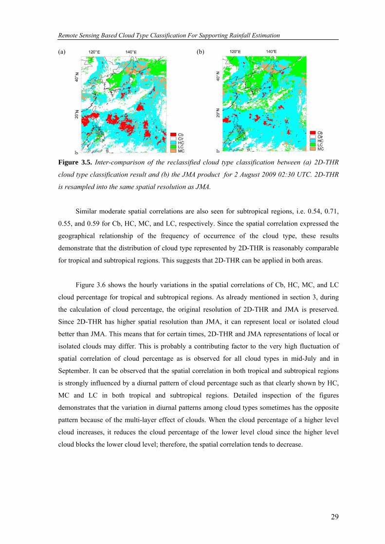
Remote Sensing Based Cloud Type Classification For Supporting Rainfall Estimation
29
(a) (b)
Figure 3.5. Inter-comparison of the reclassified cloud type classification between (a) 2D-THR
cloud type classification result and (b) the JMA product for 2 August 2009 02:30 UTC. 2D-THR
is resampled into the same spatial resolution as JMA.
Similar moderate spatial correlations are also seen for subtropical regions, i.e. 0.54, 0.71,
0.55, and 0.59 for Cb, HC, MC, and LC, respectively. Since the spatial correlation expressed the
geographical relationship of the frequency of occurrence of the cloud type, these results
demonstrate that the distribution of cloud type represented by 2D-THR is reasonably comparable
for tropical and subtropical regions. This suggests that 2D-THR can be applied in both areas.
Figure 3.6 shows the hourly variations in the spatial correlations of Cb, HC, MC, and LC
cloud percentage for tropical and subtropical regions. As already mentioned in section 3, during
the calculation of cloud percentage, the original resolution of 2D-THR and JMA is preserved.
Since 2D-THR has higher spatial resolution than JMA, it can represent local or isolated cloud
better than JMA. This means that for certain times, 2D-THR and JMA representations of local or
isolated clouds may differ. This is probably a contributing factor to the very high fluctuation of
spatial correlation of cloud percentage as is observed for all cloud types in mid-July and in
September. It can be observed that the spatial correlation in both tropical and subtropical regions
is strongly influenced by a diurnal pattern of cloud percentage such as that clearly shown by HC,
MC and LC in both tropical and subtropical regions. Detailed inspection of the figures
demonstrates that the variation in diurnal patterns among cloud types sometimes has the opposite
pattern because of the multi-layer effect of clouds. When the cloud percentage of a higher level
cloud increases, it reduces the cloud percentage of the lower level cloud since the higher level
cloud blocks the lower cloud level; therefore, the spatial correlation tends to decrease.
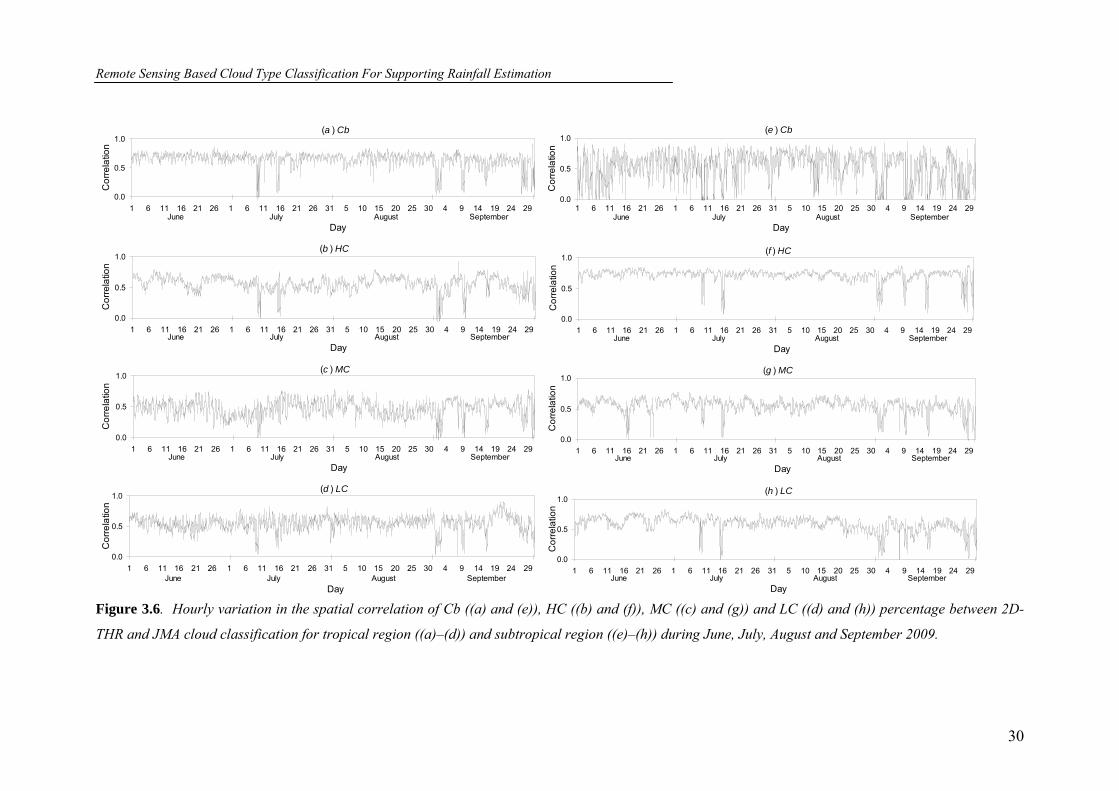
Remote Sensing Based Cloud Type Classification For Supporting Rainfall Estimation
30
(a ) Cb
0.0
0.5
1.0
1 6 11 16 21 26 1 6 11 16 21 26 31 5 10 15 20 25 30 4 9 14 19 24 29
Cor
rela
tion
June July August SeptemberDay
(e ) Cb
0.0
0.5
1.0
1 6 11 16 21 26 1 6 11 16 21 26 31 5 10 15 20 25 30 4 9 14 19 24 29
Cor
rela
tion
June July August SeptemberDay
(b ) HC
0.0
0.5
1.0
1 6 11 16 21 26 1 6 11 16 21 26 31 5 10 15 20 25 30 4 9 14 19 24 29
Cor
rela
tion
June July August SeptemberDay
(f ) HC
0.0
0.5
1.0
1 6 11 16 21 26 1 6 11 16 21 26 31 5 10 15 20 25 30 4 9 14 19 24 29
Cor
rela
tion
June July August September Day
(c ) MC
0.0
0.5
1.0
1 6 11 16 21 26 1 6 11 16 21 26 31 5 10 15 20 25 30 4 9 14 19 24 29
Cor
rela
tion
June July August SeptemberDay
(g ) MC
0.0
0.5
1.0
1 6 11 16 21 26 1 6 11 16 21 26 31 5 10 15 20 25 30 4 9 14 19 24 29
Cor
rela
tion
June July August SeptemberDay
(d ) LC
0.0
0.5
1.0
1 6 11 16 21 26 1 6 11 16 21 26 31 5 10 15 20 25 30 4 9 14 19 24 29
Cor
rela
tion
June July August SeptemberDay
(h ) LC
0.0
0.5
1.0
1 6 11 16 21 26 1 6 11 16 21 26 31 5 10 15 20 25 30 4 9 14 19 24 29
Cor
rela
tion
June July August SeptemberDay
Figure 3.6. Hourly variation in the spatial correlation of Cb ((a) and (e)), HC ((b) and (f)), MC ((c) and (g)) and LC ((d) and (h)) percentage between 2D-
THR and JMA cloud classification for tropical region ((a)–(d)) and subtropical region ((e)–(h)) during June, July, August and September 2009.
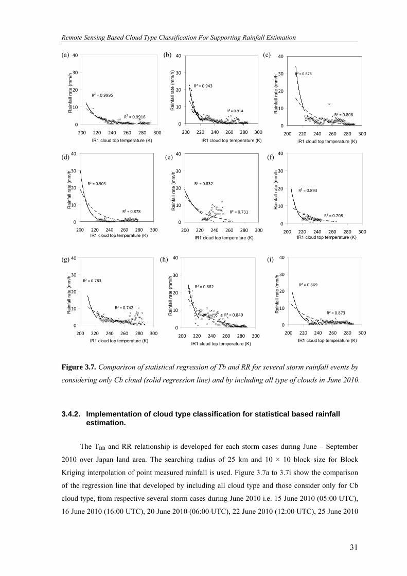
Remote Sensing Based Cloud Type Classification For Supporting Rainfall Estimation
31
R2 = 0.9916
R2 = 0.9995
0
10
20
30
40
200 220 240 260 280 300IR1 cloud top temperature (K)
Rai
nfal
l rat
e (m
m/h
)
R² = 0.914
R² = 0.943
0
10
20
30
40
200 220 240 260 280 300
Rai
nfal
l rat
e (m
m/h
)
IR1 cloud top temperature (K)
R² = 0.875
R² = 0.808
0
10
20
30
40
200 220 240 260 280 300IR1 cloud top temperature (K)
Rai
nfal
l rat
e (m
m/h
)
R² = 0.878
R² = 0.903
0
10
20
30
40
200 220 240 260 280 300IR1 cloud top temperature (K)
Rai
nfal
l rat
e (m
m/h
)
R² = 0.731
R² = 0.832
0
10
20
30
40
200 220 240 260 280 300IR1 cloud top temperature (K)
Rai
nfal
l rat
e (m
m/h
)
R² = 0.708
R² = 0.893
0
10
20
30
40
200 220 240 260 280 300IR1 cloud top temperature (K)
Rai
nfal
l rat
e (m
m/h
)
R² = 0.742
R² = 0.783
0
10
20
30
40
200 220 240 260 280 300IR1 cloud top temperature (K)
Rai
nfal
l rat
e (m
m/h
)
R² = 0.849
R² = 0.882
0
10
20
30
40
200 220 240 260 280 300IR1 cloud top temperature (K)
Rai
nfal
l rat
e (m
m/h
)
R² = 0.873
R² = 0.869
0
10
20
30
40
200 220 240 260 280 300IR1 cloud top temperature (K)
Rai
nfal
l rat
e (m
m/h
)
(a) (b) (c) (d) (e) (f) (g) (h) (i)
Figure 3.7. Comparison of statistical regression of Tb and RR for several storm rainfall events by
considering only Cb cloud (solid regression line) and by including all type of clouds in June 2010.
3.4.2. Implementation of cloud type classification for statistical based rainfall estimation.
The TBB and RR relationship is developed for each storm cases during June – September
2010 over Japan land area. The searching radius of 25 km and 10 × 10 block size for Block
Kriging interpolation of point measured rainfall is used. Figure 3.7a to 3.7i show the comparison
of the regression line that developed by including all cloud type and those consider only for Cb
cloud type, from respective several storm cases during June 2010 i.e. 15 June 2010 (05:00 UTC),
16 June 2010 (16:00 UTC), 20 June 2010 (06:00 UTC), 22 June 2010 (12:00 UTC), 25 June 2010
Remote Sensing Based Cloud Type Classification For Supporting Rainfall Estimation
32
(10:00 UTC), 26 June 2010 (03:00 UTC), 27 June 2010 (10:00 UTC), 28 June 2010 (07:00 UTC)
and 29 June 2010 (01:00 UTC).
The regression line comparison shows that the gradient of regression lines which include all
cloud type is smaller than those used Cb only. The correlation is also generally increasing for
regression which is developed only by Cb. Since the low cloud top temperature correspond to
high rainfall rate (storm event), the small gradient of regression line look likes to deliver under
estimation of estimated rainfall. Therefore by using Cb cloud type only during TIR1 and RR
relationship development this under estimation can be avoided.
3.5. SUMMARY AND CONCLUSIONS
A new 2D-THR cloud-classification algorithm has been developed; it was trained using
MAX classification results for Japan and its surrounding area. The cloud-type classification
boundary was defined by adjusting the threshold value of the distribution of mean centre of the
cloud-type clusters in the TIR1 and ΔTIR1-IR2 scatter plot. Images for northern summer (JJAS) 2009
were used for developing the 2D-THR; therefore, this diagram is typically suitable for classifying
clouds during the summer. During the adjustment process, the mean centers of certain classes
were omitted because they were included in an adjacent class. This may be considered as the main
uncertainty of this method. The presence of some areas in the 2D-THR that lack of mean centers
of cloud clusters suggests that 2D-THR should be trained by using more MAX images.
However, visual inter-comparison of a snapshot image for 2 August 2009 02:30 UTC
between a 2D-THR image and its corresponding night-time microphysical color composite image,
shows that most of cloud types identified in the color composite image were well represented in
the2D-THR image. Inter-comparison of the JMA image and 2D-THR for the same period also
proves good visual agreement between the two.
The cloud percentages for JMA and 2D-THR during JJAS 2009 over tropical and
subtropical regions were spatially correlated. The results showed that the geographical
distribution of the frequency of occurrence of each cloud type is moderately represented by 2D-
THR. It suggests that 2D-THR can be reasonably applied for tropical and subtropical regions. 2D-
THR has higher spatial resolution than JMA; hence, it can represent local or isolated cloud better
than JMA. However, its cloud-type representation is different. The graphical comparison of the
spatial correlation of cloud percentage during JJAS 2009 demonstrates very high fluctuation of
spatial correlation for certain times; this fluctuation is most probably caused by different

Remote Sensing Based Cloud Type Classification For Supporting Rainfall Estimation
33
representations of the local cloud type. The graph also showed opposite patterns of diurnal
variation among the cloud types because of a multilayer cloud effect.
Integrating the cloud type classification especially by separating Cb cloud type from other
cloud types can improve the TIR1 and RR relationship as well as rainfall estimation, which is
indicated by increasing correlation coefficient and the gradient of regression line. Moreover,
underestimating rainfall intensity can be avoided by applying TIR1 and RR relationship that uses
Cb cloud type only rather than using all cloud types.
Chapter 4. THE USE OF GEOSTATIONARY BASED RAINFALL ESTIMATION FOR CHARACTERIZING STORM SEVERITY
This chapter is based on: Suseno, Dwi Prabowo Yuga, T. J. Yamada, 2012, The use of geostationary
based rainfall estimation for characterizing strom severity, Journal of Japan Society of Civil Engineers,
Ser. B1 (Hydraulic Engineering), Volume 68, Issue 4, pp. I_175-I_180

The Use Of Geostationary Based Rainfall Estimation For Characterizing Storm Severity
35
Abstract
This study deals with the use of geostationary satellite based rainfall estimation for
characterizing storm severity. The objectives of this study are to estimate storm rainfall intensity
by using Multi-functional Transport Satellite (MTSAT) blended with C-band rainfall radar data
and to show the severity of the identified storm rainfall intensity by representing its return period
map. A regional frequency analysis (RFA) method developed by Hosking and Wallis (1997) is
used to define the frequency distribution of long-term hourly maximum rainfall over Hokkaido
Island. RFA indicates that Generalized Normal/Log Normal Three Parameters (GNO/LN3) is
suitable to describe the frequency distribution of long-term hourly maximum rainfall over
Hokkaido Island. Based on that frequency distribution, characterization of severity of 23 August
2010 storm event has been performed over western part of Hokkaido Island using MTSAT
rainfall estimation. This comparison demonstrates that that the return period information shown
by MTSAT rainfall is comparable with AMeDAS rainfall return period. For assessing the return
period of an extreme event in the area that observed rainfall is lacking, the use of geostationary
satellite based is proved useful to overcome such problem.
Key Words: MTSAT, C-band radar, Rainfall estimation, Regional Frequency Analysis
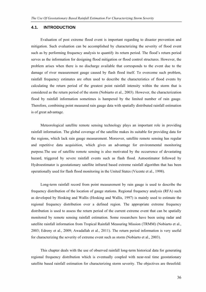
The Use Of Geostationary Based Rainfall Estimation For Characterizing Storm Severity
36
4.1. INTRODUCTION
Evaluation of post extreme flood event is important regarding to disaster prevention and
mitigation. Such evaluation can be accomplished by characterizing the severity of flood event
such as by performing frequency analysis to quantify its return period. The flood’s return period
serves as the information for designing flood mitigation or flood control structures. However, the
problem arises when there is no discharge available that corresponds to the event due to the
damage of river measurement gauge caused by flash flood itself. To overcome such problem,
rainfall frequency estimates are often used to describe the characteristics of flood events by
calculating the return period of the greatest point rainfall intensity within the storm that is
considered as the return period of the storm (Nobiarto et al., 2003). However, the characterization
flood by rainfall information sometimes is hampered by the limited number of rain gauge.
Therefore, combining point measured rain gauge data with spatially distributed rainfall estimation
is of great advantage.
Meteorological satellite remote sensing technology plays an important role in providing
rainfall information. The global coverage of the satellite makes its suitable for providing data for
the regions, which lack rain gauge measurement. Moreover, satellite remote sensing has regular
and repetitive data acquisition, which gives an advantage for environmental monitoring
purpose.The use of satellite remote sensing is also motivated by the occurrence of devastating
hazard, triggered by severe rainfall events such as flash flood. Autoestimator followed by
Hydroestimator is geostationary satellite infrared based extreme rainfall algorithm that has been
operationally used for flash flood monitoring in the United States (Vicente et al., 1998).
Long-term rainfall record from point measurement by rain gauge is used to describe the
frequency distribution of the location of gauge stations. Regional frequency analysis (RFA) such
as developed by Hosking and Wallis (Hosking and Wallis, 1997) is mainly used to estimate the
regional frequency distribution over a defined region. The appropriate extreme frequency
distribution is used to assess the return period of the current extreme event that can be spatially
monitored by remote sensing rainfall estimation. Some researchers have been using radar and
satellite rainfall information from Tropical Rainfall Measuring Mission (TRMM) (Nobiarto et al.,
2003; Edreny et al., 2009; Awadallah et al., 2011). The return period information is very useful
for characterizing the severity of extreme event such as storm (Nobiarto et al., 2003).
This chapter deals with the use of observed rainfall long-term historical data for generating
regional frequency distribution which is eventually coupled with near-real time geostationary
satellite based rainfall estimation for characterizing storm severity. The objectives are threefold:
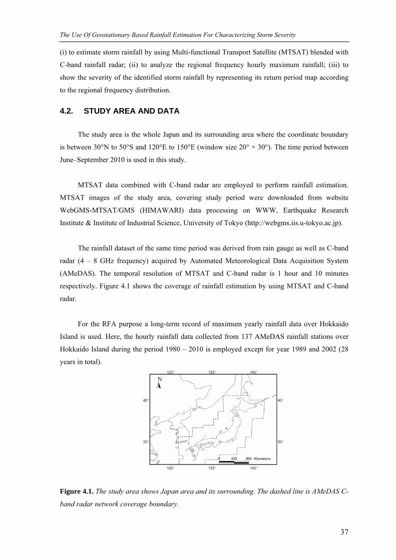
The Use Of Geostationary Based Rainfall Estimation For Characterizing Storm Severity
37
(i) to estimate storm rainfall by using Multi-functional Transport Satellite (MTSAT) blended with
C-band rainfall radar; (ii) to analyze the regional frequency hourly maximum rainfall; (iii) to
show the severity of the identified storm rainfall by representing its return period map according
to the regional frequency distribution.
4.2. STUDY AREA AND DATA
The study area is the whole Japan and its surrounding area where the coordinate boundary
is between 30°N to 50°S and 120°E to 150°E (window size 20° × 30°). The time period between
June–September 2010 is used in this study.
MTSAT data combined with C-band radar are employed to perform rainfall estimation.
MTSAT images of the study area, covering study period were downloaded from website
WebGMS-MTSAT/GMS (HIMAWARI) data processing on WWW, Earthquake Research
Institute & Institute of Industrial Science, University of Tokyo (http://webgms.iis.u-tokyo.ac.jp).
The rainfall dataset of the same time period was derived from rain gauge as well as C-band
radar (4 – 8 GHz frequency) acquired by Automated Meteorological Data Acquisition System
(AMeDAS). The temporal resolution of MTSAT and C-band radar is 1 hour and 10 minutes
respectively. Figure 4.1 shows the coverage of rainfall estimation by using MTSAT and C-band
radar.
For the RFA purpose a long-term record of maximum yearly rainfall data over Hokkaido
Island is used. Here, the hourly rainfall data collected from 137 AMeDAS rainfall stations over
Hokkaido Island during the period 1980 – 2010 is employed except for year 1989 and 2002 (28
years in total).
Figure 4.1. The study area shows Japan area and its surrounding. The dashed line is AMeDAS C-
band radar network coverage boundary.
The Use Of Geostationary Based Rainfall Estimation For Characterizing Storm Severity
38
4.3. METHODS
The methodology of this study contains two main parts; the first satellite rainfall estimation
by using MTSAT satellite datasets and the second regional frequency analysis by using Hosking
and Wallis method (1997). Figure 4.2 shows the brief flow chart of the study and next section is
the explanation of such diagram.
4.3.1. Satellite rainfall estimation
The satellite rainfall estimation by using geostationary satellite is based on an indirect
relationship between cloud top temperature depicted by infrared (IR-10.8 μm) channel and rainfall
rate (RR) derived by another devices. Misra et. al. uses IR data from Indian Satellite (INSAT-1D)
and rainfall intensity form rain gauge measurement to show the IR and RR relationship (Misra et
al., 2001).
Figure 4.2. MTSAT based rainfall estimation and return period mapping methodology used in
this study.
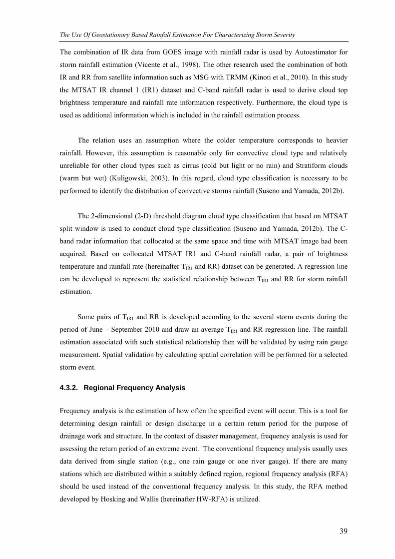
The Use Of Geostationary Based Rainfall Estimation For Characterizing Storm Severity
39
The combination of IR data from GOES image with rainfall radar is used by Autoestimator for
storm rainfall estimation (Vicente et al., 1998). The other research used the combination of both
IR and RR from satellite information such as MSG with TRMM (Kinoti et al., 2010). In this study
the MTSAT IR channel 1 (IR1) dataset and C-band rainfall radar is used to derive cloud top
brightness temperature and rainfall rate information respectively. Furthermore, the cloud type is
used as additional information which is included in the rainfall estimation process.
The relation uses an assumption where the colder temperature corresponds to heavier
rainfall. However, this assumption is reasonable only for convective cloud type and relatively
unreliable for other cloud types such as cirrus (cold but light or no rain) and Stratiform clouds
(warm but wet) (Kuligowski, 2003). In this regard, cloud type classification is necessary to be
performed to identify the distribution of convective storms rainfall (Suseno and Yamada, 2012b).
The 2-dimensional (2-D) threshold diagram cloud type classification that based on MTSAT
split window is used to conduct cloud type classification (Suseno and Yamada, 2012b). The C-
band radar information that collocated at the same space and time with MTSAT image had been
acquired. Based on collocated MTSAT IR1 and C-band rainfall radar, a pair of brightness
temperature and rainfall rate (hereinafter TIR1 and RR) dataset can be generated. A regression line
can be developed to represent the statistical relationship between TIR1 and RR for storm rainfall
estimation.
Some pairs of TIR1 and RR is developed according to the several storm events during the
period of June – September 2010 and draw an average TIR1 and RR regression line. The rainfall
estimation associated with such statistical relationship then will be validated by using rain gauge
measurement. Spatial validation by calculating spatial correlation will be performed for a selected
storm event.
4.3.2. Regional Frequency Analysis
Frequency analysis is the estimation of how often the specified event will occur. This is a tool for
determining design rainfall or design discharge in a certain return period for the purpose of
drainage work and structure. In the context of disaster management, frequency analysis is used for
assessing the return period of an extreme event. The conventional frequency analysis usually uses
data derived from single station (e.g., one rain gauge or one river gauge). If there are many
stations which are distributed within a suitably defined region, regional frequency analysis (RFA)
should be used instead of the conventional frequency analysis. In this study, the RFA method
developed by Hosking and Wallis (hereinafter HW-RFA) is utilized.

The Use Of Geostationary Based Rainfall Estimation For Characterizing Storm Severity
40
The first step of HW-RFA is data screening. The purpose of screening the data is to
eliminate the gross error and inconsistencies and to check whether the data are homogeneous
(stationary) over time. Generally the hydrometeorological data is available in small size of sample,
therefore in HW-RFA the concept of L-moment is introduced. L moment are based on
probability-weighted moment (PWM). The rth PWM, βr is defined as
∫∞
∞−
=
≡
dxxfxFx
XFXE
xr
x
rXr
).(.)](.[
})](.[{β (4.1)
where Fx is cumulative distribution function (CDF) and fx is probability distribution function
(PDF).
The first four moment are computed as
)5.4(.12.30.20)4.4(.6.6)3.4(.2)2.4(
01134
0113
012
01
ββββλβββλ
ββλβλ
−+−=+−=
−==
where λ1 is the first moment (mean), λ2 is the second moment (variance), λ3 is the third
moment (skewness) and λ4 is the fourth moment (kurtosis). Some dimensionless ratios can also be
defined as ratio of L-moment that are analogous to the coefficient of variation, skewness and
kurtosis as following
)8.4(:)(
)7.4(:)(
)6.4(:)(var
2
44
2
33
1
22
λλ
τ
λλ
τ
λλ
τ
≡−
≡−
≡−
LCkkurtosisoftcoefficienL
LCsskewnessoftcoefficienL
LCviationoftcoefficienL
For screening the data, the discordancy measure (Di) is used. The Di is defined by:
(4.9)
where ui is the vector of L-moments i.e. L-coefficient of variation (LCv), L-coefficient of
skewness (LCs) and L-coefficient of kurtosis (LCk) for a site i. S is defined by
(4.10)
(4.11)
)()(31 1 uuSuuD i
Tii −−= −
∑=
−=sN
iis uNu
1
1
∑=
− −−−=sN
i
Tiis uuuuNS
1
1 ))(()1(

The Use Of Geostationary Based Rainfall Estimation For Characterizing Storm Severity
41
where Ns is the number of sites in the group. A site is denoted as discordant if Di > 3.
The next step is the identification of homogeneous region. Homogeneous region is
considered as a set of sites whose frequency distributions are considered to be approximately the
same. This ‘region’ is the fundamental unit of RFA. A heterogeneity measured is called H-
statistic which is defined as follow
v
vVH
σμ )( −
= (4.12)
where vμ is mean of simulation, vσ is standard deviation of simulation and V is
observed dispersion which are measured as to LCv scatter, LCv-LCs and LCv-LCk, therefore
three heterogeneity measures called H1, H2 and H3 that corresponds to LCv scatter, LCv-LCs and
LCv-LCk respectively. However H1 is commonly used. In general a region is declared ‘acceptably
homogeneous’ if H1 < 1, ‘possibly heterogeneous’ if 1 ≤ H1 < 2, and definitely heterogeneous’
if H1 > 2.
An appropriate frequency distribution is chosen by inspecting the goodness of fit between
LCk versus LCs for various commonly used distributions duration with the corresponding relation
obtained from the at site and regional data. This process is performed by using the Z-statistic as
well as graphical method (LCs and LCk diagram).
Once an appropriate frequency distribution is selected, the distribution parameters such as
shape, location and scaled can be calculated and the CDF; Fx can be defined. The exceedance
probability of an extreme event; x can be calculated based on the CDF and eventually the return
period (RP) is calculated as
xF
RP−
=1
1 (4.13)
4.4. RESULTS AND DISCUSSIONS
4.4.1. Rainfall estimation based on BT and RR statistical relationship
During the period June – September 2010, heavy rainfall event cases was selected by
inspecting both rain gauge measurement data as well as MTSAT image to select storm rainfall
events. According to the inspection, it was notified that storm events strongly correspond to the
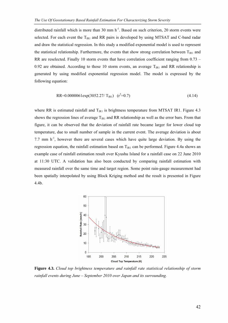
The Use Of Geostationary Based Rainfall Estimation For Characterizing Storm Severity
42
distributed rainfall which is more than 30 mm h-1. Based on such criterion, 20 storm events were
selected. For each event the TIR1 and RR pairs is developed by using MTSAT and C-band radar
and draw the statistical regression. In this study a modified exponential model is used to represent
the statistical relationship. Furthermore, the events that show strong correlation between TIR1 and
RR are reselected. Finally 10 storm events that have correlation coefficient ranging from 0.73 –
0.92 are obtained. According to those 10 storm events, an average TIR1 and RR relationship is
generated by using modified exponential regression model. The model is expressed by the
following equation:
RR=0.0000061exp(3052.27/ TIR1) (r2=0.7) (4.14)
where RR is estimated rainfall and TIR1 is brightness temperature from MTSAT IR1. Figure 4.3
shows the regression lines of average TIR1 and RR relationship as well as the error bars. From that
figure, it can be observed that the deviation of rainfall rate became larger for lower cloud top
temperature, due to small number of sample in the current event. The average deviation is about
7.7 mm h-1, however there are several cases which have quite large deviation. By using the
regression equation, the rainfall estimation based on TIR1 can be performed. Figure 4.4a shows an
example case of rainfall estimation result over Kyushu Island for a rainfall case on 22 June 2010
at 11:30 UTC. A validation has also been conducted by comparing rainfall estimation with
measured rainfall over the same time and target region. Some point rain-gauge measurement had
been spatially interpolated by using Block Kriging method and the result is presented in Figure
4.4b.
Figure 4.3. Cloud top brightness temperature and rainfall rate statistical relationship of storm
rainfall events during June – September 2010 over Japan and its surrounding.
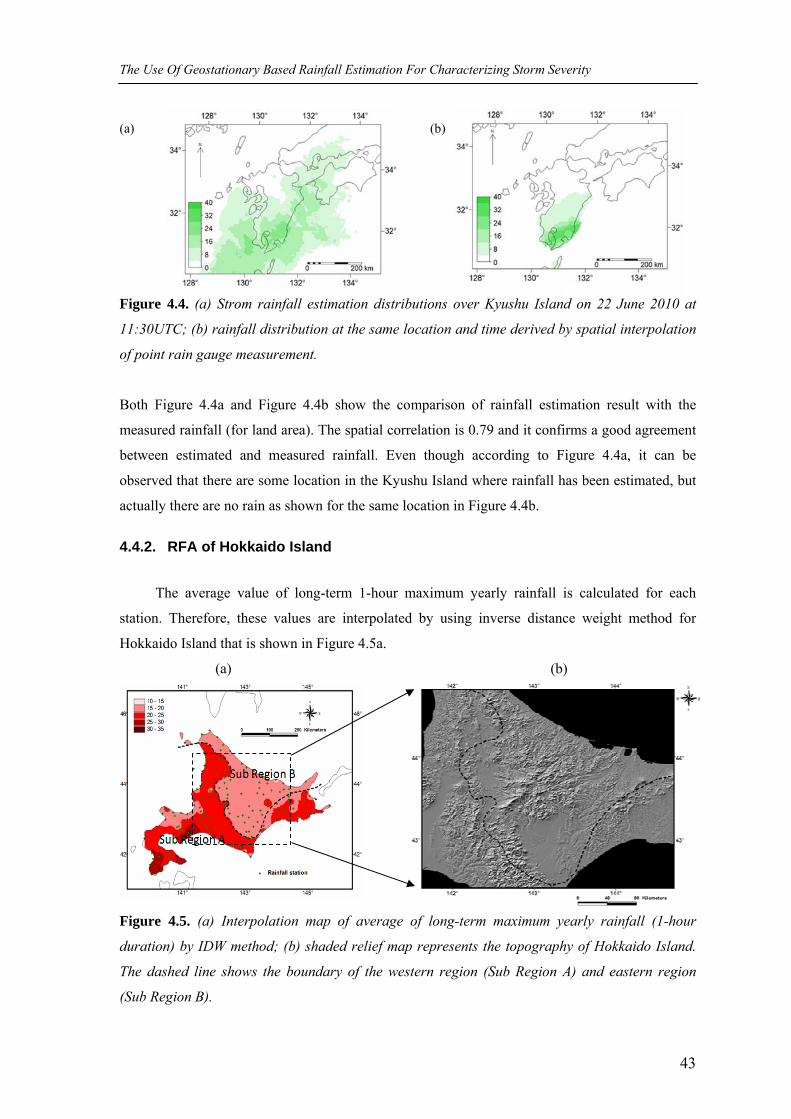
The Use Of Geostationary Based Rainfall Estimation For Characterizing Storm Severity
43
(a) (b)
Figure 4.4. (a) Strom rainfall estimation distributions over Kyushu Island on 22 June 2010 at
11:30UTC; (b) rainfall distribution at the same location and time derived by spatial interpolation
of point rain gauge measurement.
Both Figure 4.4a and Figure 4.4b show the comparison of rainfall estimation result with the
measured rainfall (for land area). The spatial correlation is 0.79 and it confirms a good agreement
between estimated and measured rainfall. Even though according to Figure 4.4a, it can be
observed that there are some location in the Kyushu Island where rainfall has been estimated, but
actually there are no rain as shown for the same location in Figure 4.4b.
4.4.2. RFA of Hokkaido Island
The average value of long-term 1-hour maximum yearly rainfall is calculated for each
station. Therefore, these values are interpolated by using inverse distance weight method for
Hokkaido Island that is shown in Figure 4.5a.
(a) (b)
Figure 4.5. (a) Interpolation map of average of long-term maximum yearly rainfall (1-hour
duration) by IDW method; (b) shaded relief map represents the topography of Hokkaido Island.
The dashed line shows the boundary of the western region (Sub Region A) and eastern region
(Sub Region B).
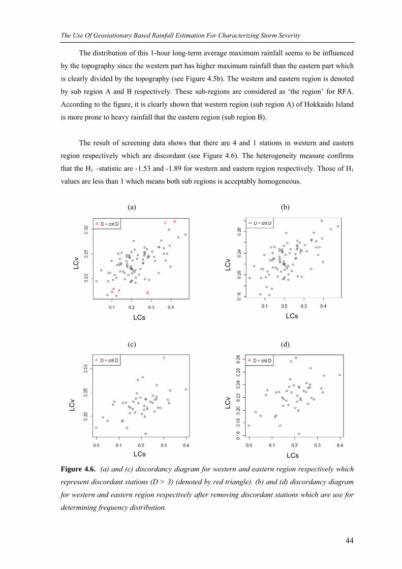
The Use Of Geostationary Based Rainfall Estimation For Characterizing Storm Severity
44
The distribution of this 1-hour long-term average maximum rainfall seems to be influenced
by the topography since the western part has higher maximum rainfall than the eastern part which
is clearly divided by the topography (see Figure 4.5b). The western and eastern region is denoted
by sub region A and B respectively. These sub-regions are considered as ‘the region’ for RFA.
According to the figure, it is clearly shown that western region (sub region A) of Hokkaido Island
is more prone to heavy rainfall that the eastern region (sub region B).
The result of screening data shows that there are 4 and 1 stations in western and eastern
region respectively which are discordant (see Figure 4.6). The heterogeneity measure confirms
that the H1 –statistic are -1.53 and -1.89 for western and eastern region respectively. Those of H1
values are less than 1 which means both sub regions is acceptably homogeneous.
(a)
(b)
(c)
(d)
Figure 4.6. (a) and (c) discordancy diagram for western and eastern region respectively which
represent discordant stations (D > 3) (denoted by red triangle). (b) and (d) discordancy diagram
for western and eastern region respectively after removing discordant stations which are use for
determining frequency distribution.
LCs
LCs
LCs
LCs
LCv
LCv
LCv
LCv
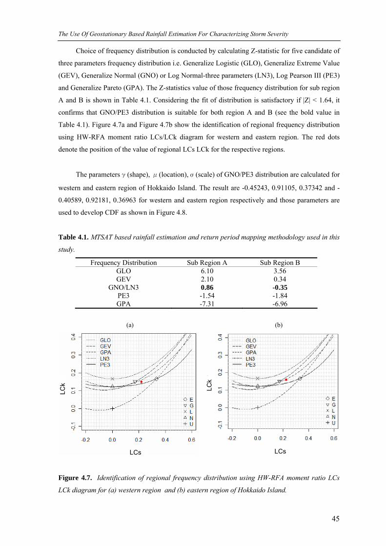
The Use Of Geostationary Based Rainfall Estimation For Characterizing Storm Severity
45
Choice of frequency distribution is conducted by calculating Z-statistic for five candidate of
three parameters frequency distribution i.e. Generalize Logistic (GLO), Generalize Extreme Value
(GEV), Generalize Normal (GNO) or Log Normal-three parameters (LN3), Log Pearson III (PE3)
and Generalize Pareto (GPA). The Z-statistics value of those frequency distribution for sub region
A and B is shown in Table 4.1. Considering the fit of distribution is satisfactory if |Z| < 1.64, it
confirms that GNO/PE3 distribution is suitable for both region A and B (see the bold value in
Table 4.1). Figure 4.7a and Figure 4.7b show the identification of regional frequency distribution
using HW-RFA moment ratio LCs/LCk diagram for western and eastern region. The red dots
denote the position of the value of regional LCs LCk for the respective regions.
The parametersγ(shape), μ(location),σ(scale) of GNO/PE3 distribution are calculated for
western and eastern region of Hokkaido Island. The result are -0.45243, 0.91105, 0.37342 and -
0.40589, 0.92181, 0.36963 for western and eastern region respectively and those parameters are
used to develop CDF as shown in Figure 4.8.
Table 4.1. MTSAT based rainfall estimation and return period mapping methodology used in this
study.
Frequency Distribution Sub Region A Sub Region B GLO 6.10 3.56 GEV 2.10 0.34
GNO/LN3 0.86 -0.35 PE3 -1.54 -1.84 GPA -7.31 -6.96
(a)
(b)
Figure 4.7. Identification of regional frequency distribution using HW-RFA moment ratio LCs
LCk diagram for (a) western region and (b) eastern region of Hokkaido Island.
LCs LCs
LCk
LCk
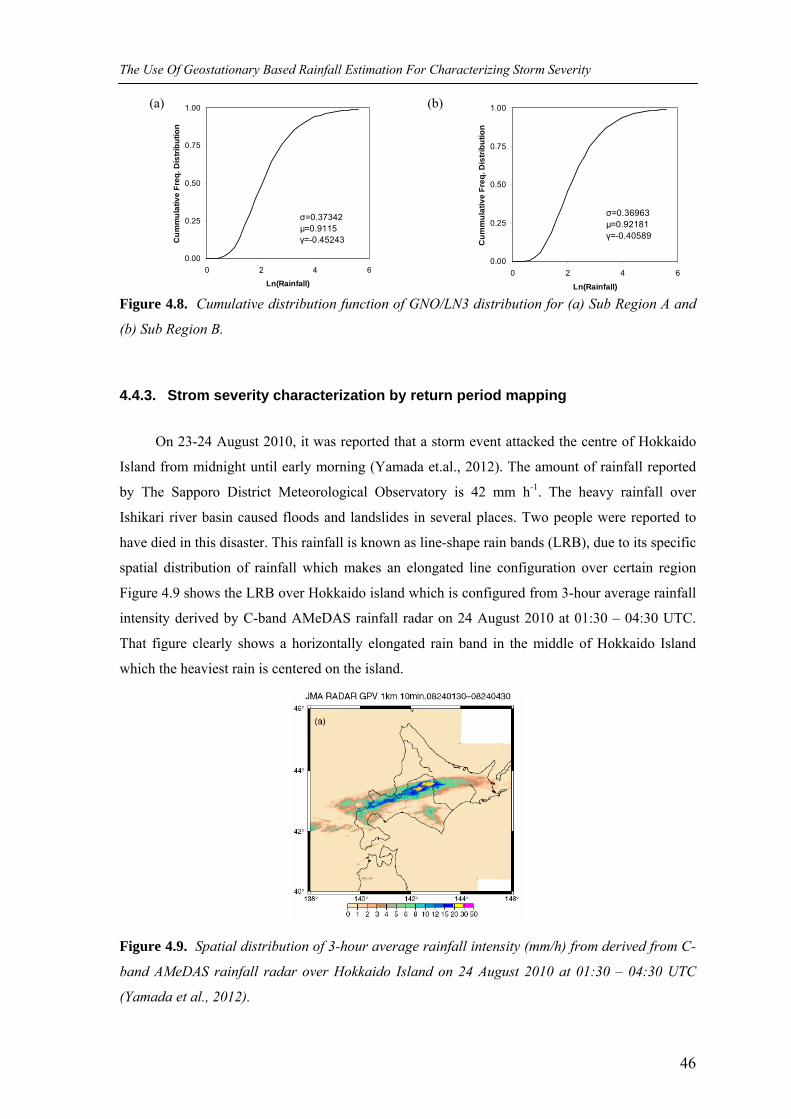
The Use Of Geostationary Based Rainfall Estimation For Characterizing Storm Severity
46
0.00
0.25
0.50
0.75
1.00
0 2 4 6
Ln(Rainfall)
Cum
mul
ativ
e Fr
eq. D
istri
butio
n
σ=0.37342μ=0.9115γ=-0.45243
0.00
0.25
0.50
0.75
1.00
0 2 4 6
Ln(Rainfall)
Cum
mul
ativ
e Fr
eq. D
istri
butio
n
σ=0.36963μ=0.92181γ=-0.40589
(a) (b)
Figure 4.8. Cumulative distribution function of GNO/LN3 distribution for (a) Sub Region A and
(b) Sub Region B.
4.4.3. Strom severity characterization by return period mapping
On 23-24 August 2010, it was reported that a storm event attacked the centre of Hokkaido
Island from midnight until early morning (Yamada et.al., 2012). The amount of rainfall reported
by The Sapporo District Meteorological Observatory is 42 mm h-1. The heavy rainfall over
Ishikari river basin caused floods and landslides in several places. Two people were reported to
have died in this disaster. This rainfall is known as line-shape rain bands (LRB), due to its specific
spatial distribution of rainfall which makes an elongated line configuration over certain region
Figure 4.9 shows the LRB over Hokkaido island which is configured from 3-hour average rainfall
intensity derived by C-band AMeDAS rainfall radar on 24 August 2010 at 01:30 – 04:30 UTC.
That figure clearly shows a horizontally elongated rain band in the middle of Hokkaido Island
which the heaviest rain is centered on the island.
Figure 4.9. Spatial distribution of 3-hour average rainfall intensity (mm/h) from derived from C-
band AMeDAS rainfall radar over Hokkaido Island on 24 August 2010 at 01:30 – 04:30 UTC
(Yamada et al., 2012).
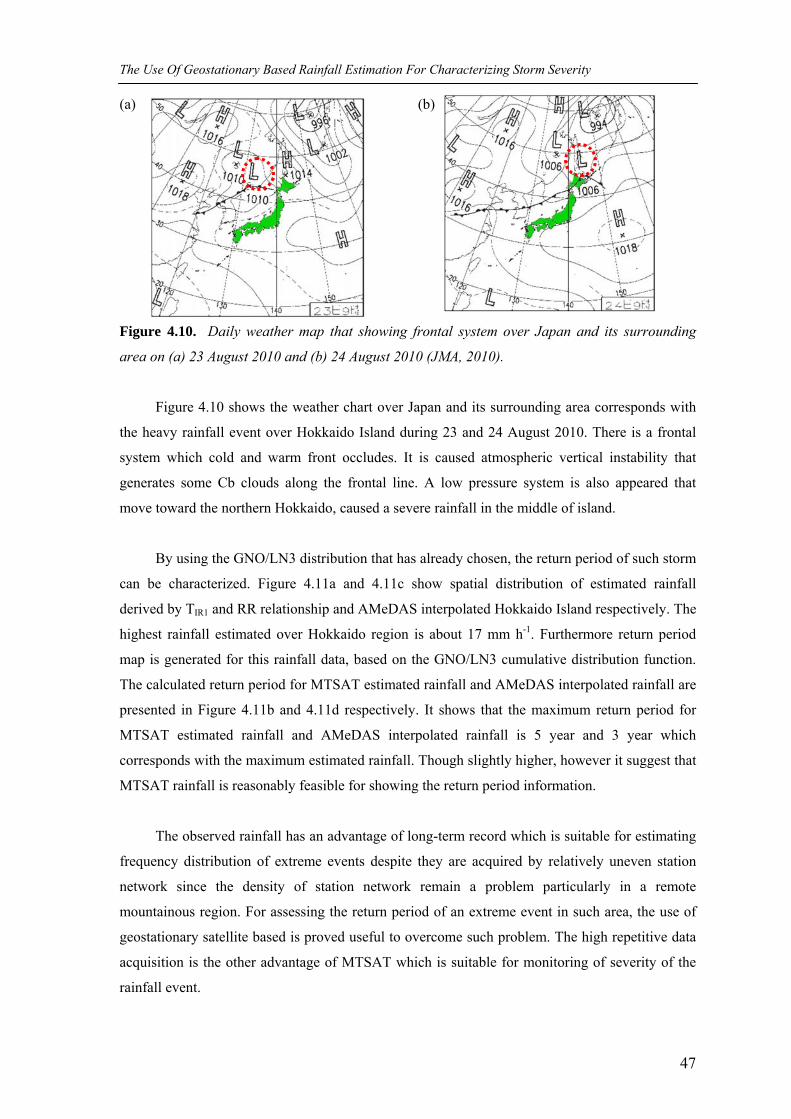
The Use Of Geostationary Based Rainfall Estimation For Characterizing Storm Severity
47
(a) (b)
Figure 4.10. Daily weather map that showing frontal system over Japan and its surrounding
area on (a) 23 August 2010 and (b) 24 August 2010 (JMA, 2010).
Figure 4.10 shows the weather chart over Japan and its surrounding area corresponds with
the heavy rainfall event over Hokkaido Island during 23 and 24 August 2010. There is a frontal
system which cold and warm front occludes. It is caused atmospheric vertical instability that
generates some Cb clouds along the frontal line. A low pressure system is also appeared that
move toward the northern Hokkaido, caused a severe rainfall in the middle of island.
By using the GNO/LN3 distribution that has already chosen, the return period of such storm
can be characterized. Figure 4.11a and 4.11c show spatial distribution of estimated rainfall
derived by TIR1 and RR relationship and AMeDAS interpolated Hokkaido Island respectively. The
highest rainfall estimated over Hokkaido region is about 17 mm h-1. Furthermore return period
map is generated for this rainfall data, based on the GNO/LN3 cumulative distribution function.
The calculated return period for MTSAT estimated rainfall and AMeDAS interpolated rainfall are
presented in Figure 4.11b and 4.11d respectively. It shows that the maximum return period for
MTSAT estimated rainfall and AMeDAS interpolated rainfall is 5 year and 3 year which
corresponds with the maximum estimated rainfall. Though slightly higher, however it suggest that
MTSAT rainfall is reasonably feasible for showing the return period information.
The observed rainfall has an advantage of long-term record which is suitable for estimating
frequency distribution of extreme events despite they are acquired by relatively uneven station
network since the density of station network remain a problem particularly in a remote
mountainous region. For assessing the return period of an extreme event in such area, the use of
geostationary satellite based is proved useful to overcome such problem. The high repetitive data
acquisition is the other advantage of MTSAT which is suitable for monitoring of severity of the
rainfall event.
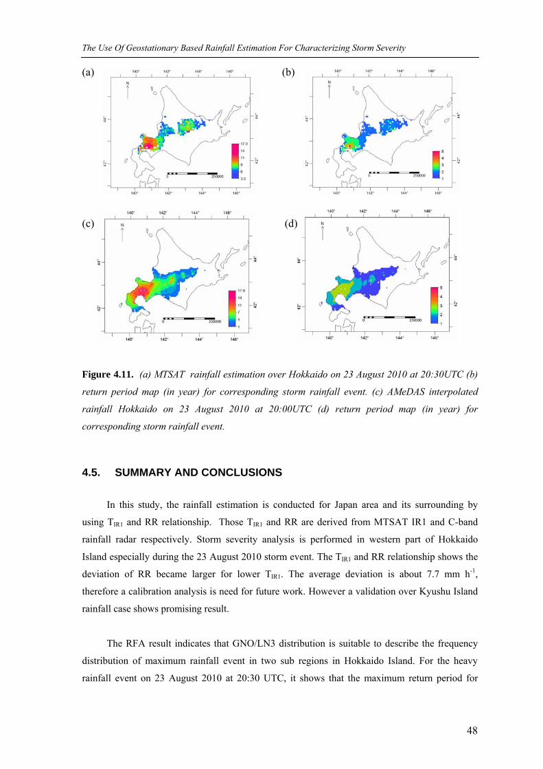
The Use Of Geostationary Based Rainfall Estimation For Characterizing Storm Severity
48
(a) (b)
(c) (d)
Figure 4.11. (a) MTSAT rainfall estimation over Hokkaido on 23 August 2010 at 20:30UTC (b)
return period map (in year) for corresponding storm rainfall event. (c) AMeDAS interpolated
rainfall Hokkaido on 23 August 2010 at 20:00UTC (d) return period map (in year) for
corresponding storm rainfall event.
4.5. SUMMARY AND CONCLUSIONS
In this study, the rainfall estimation is conducted for Japan area and its surrounding by
using TIR1 and RR relationship. Those TIR1 and RR are derived from MTSAT IR1 and C-band
rainfall radar respectively. Storm severity analysis is performed in western part of Hokkaido
Island especially during the 23 August 2010 storm event. The TIR1 and RR relationship shows the
deviation of RR became larger for lower TIR1. The average deviation is about 7.7 mm h-1,
therefore a calibration analysis is need for future work. However a validation over Kyushu Island
rainfall case shows promising result.
The RFA result indicates that GNO/LN3 distribution is suitable to describe the frequency
distribution of maximum rainfall event in two sub regions in Hokkaido Island. For the heavy
rainfall event on 23 August 2010 at 20:30 UTC, it shows that the maximum return period for

The Use Of Geostationary Based Rainfall Estimation For Characterizing Storm Severity
49
MTSAT estimated rainfall and AMeDAS interpolated rainfall is 5 year and 3 year which
corresponds with the maximum estimated rainfall.
The observed rainfall has an advantage of long-term record which is suitable for estimating
frequency distribution of extreme events despite they are acquired by relatively uneven station
network since the density of station network remain a problem particularly in a remote
mountainous region. For assessing the return period of an extreme event in such area, the use of
geostationary satellite based is proved useful to overcome such problem. The high repetitive data
acquisition is the other advantage of MTSAT which is suitable for monitoring of severity of the
rainfall event.
Chapter 5. INTEGRATION OF ATMOSPHERIC ENVIRONMENTAL CONDITIONS INTO GEOSTATIONARY SATELLITE BASED RAINFALL ESTIMATION
This chapter is based on: Suseno, Dwi Prabowo Yuga, T. J. Yamada, 2013, The role of precipitable water
vapor and atmospheric stability index in the statistically-based rainfall estimation using MTSAT data,
Journal of Hydrometeorology (accepted).
Integration Of Atmospheric Environmental Condition Into Geostationary Satellite Based Rainfall Estimation
51
Abstract
A rainfall estimation method was developed based on the statistical relationships
between cloud top temperature and rainfall rates acquired by both the 10.8 µm channel of the
Multi-functional Transport Satellite (MTSAT) series and the Automated Meteorological Data
Acquisition System (AMeDAS) C-band radar, respectively. The method focused on
cumulonimbus (Cb) clouds and was developed in the period of June–September 2010 and 2011,
over the landmass of Japan and its surrounding area. Total precipitable water vapor (PWV) and
atmospheric vertical instability were considered to represent the atmospheric environmental
conditions during the development of statistical models. Validations were performed by
comparing the estimated values with the observed rainfall derived from the AMeDAS rain gauge
network and the Tropical Rainfall Measuring Mission (TRMM) 3B42 rainfall estimation product.
The results demonstrated that the models that considered the combination of total PWV and
atmospheric vertical instability were relatively more sensitive to heavy rainfall than were the
models that considered no atmospheric environmental conditions. The use of such combined
information indicated a reasonable improvement, especially in terms of the correlation between
estimated and observed rainfall. Intercomparison results with the TRMM 3B42 confirmed that
MTSAT-based rainfall estimations made by considering atmospheric environmental conditions
were more accurate for estimating rainfall generated by Cb cloud.
Keywords: MTSAT, rainfall estimation, Precipitable Water Vapor, Atmospheric vertical
instability
Integration Of Atmospheric Environmental Condition Into Geostationary Satellite Based Rainfall Estimation
52
5.1. INTRODUCTION
Geostationary satellites make frequent observations with continuous spatial coverage,
providing useful information for rainfall monitoring and the early warning of storms (Feidas et al.
2001; Wardah et al. 2003). Thermal infrared data (TIR) centered at 10.8 µm are commonly used
to detect cloud top temperature for use in rainfall estimation (Haile et al. 2010). Lower
temperatures are assumed to correspond to relatively cold and thick clouds, which tend to produce
high rainfall intensity (Kuligowski, 2003). However, clouds are essentially opaque to TIR, which
cannot reveal the vertical profile of clouds that produce rainfall. To complement TIR data,
microwave (MW)-based rainfall estimations are used, as MW has the ability to penetrate clouds
and allows the measurement of aspects of the hydrometeor field. Several well-known algorithms
have advantages when using complementary information in TIR and MW data, such as the
Precipitation Estimation from Remotely Sensed Information using Artificial Neural Networks
(PERSIANN; Sorooshian et al. 2000) and the Tropical Rainfall Measuring Mission (TRMM)
3B42 (Huffman et al. 2007). These products are easily accessible through their dedicated server
via the Internet and can be used for water resource management purposes. However, the products
are mainly delivered at 0.25° and 3 hourly spatial and temporal resolutions, respectively, which
are relatively too coarse for certain hydrological applications such as the detection of flash floods
in small ungauged catchments. The aim of this study was to develop a rainfall estimation method
based on a combination of TIR and MW that can be applied for the monitoring of flash floods;
hence, rainfall information with high temporal resolution is necessary.
To combine TIR and MW for rainfall estimation, a statistical model that represents the
relationship between them is commonly implemented (Vicente et al. 1998; Haile et al. 2010;
Kinoti et al. 2010). Rainfall estimation using a TIR and MW statistical model as a function of TIR
is considered to be suitable for convective clouds, but not suitable for non-convective clouds
(Kuligowski 2003). For separating convective and non-convective clouds, cloud classification
data should be considered during the development of the TIR and MW statistical model (Suseno
and Yamada, 2012b). However, the use of a single statistical model for the estimation of rainfall
is limited due to the variety of physical processes associated with rainfall generation, which
eventually influence the relationship between cloud top temperature and rainfall rates (Vicente et
al. 1998). According to Doswell et al. (1996), deep moist convection normally occurs during the
warm season, when high moisture content is possible and buoyant instability promotes strong
upward vertical motions. In this study, PWV and atmospheric vertical instability, which are both
related to the development of deep convective cloud, were investigated. The objectives of the
study were to assess how a combination of total PWV and atmospheric vertical instability
conditions improves TIR-based rainfall estimations using a statistical model by focusing on Cb
Integration Of Atmospheric Environmental Condition Into Geostationary Satellite Based Rainfall Estimation
53
cloud systems and to validate the estimated rainfall by comparison with observed rainfall during
convective storm rainfall events.
5.2. STUDY AREA AND MATERIALS
The study area was Japan and its surrounding area between 30–50°N and 120–150°E
(window size 20° × 30°). The two time periods examined were June–September of 2010 and 2011.
The collocated data pairs (i.e., obtained in the same geographical area during the same time
periods) of TIR and MW were used to develop a statistical model for the estimation of rainfall.
TIR images were acquired from the Multi-functional Transport Satellite (MTSAT), particularly
from the 10.8 µm channel (TIR1). The MW-based rainfall rate observations were derived from the
Automated Meteorological Data Acquisition System (AMeDAS) C-band radar data (RR). The
12.0-µm MTSAT image channel (TIR2) was used in conjunction with TIR1 to develop a cloud-type
classification system and cloud height images. In the study region, the spatial resolution of
MTSAT data was approximately 5 × 5 km. The temporal resolutions of the MTSAT and C-band
radar data were 1 hour and 10 minutes, respectively.
Relative humidity derived from rawinsonde data is suitable to represent the moisture factor
and was used by Vicente et al. (1998). However, such data have limitations in their spatial and
temporal sampling. Therefore, a PWV estimated from ground-based GPS networks to represent
the total PWV is used. These data can offer spatiotemporal improvements in moisture observation
when compared with radiosonde observations (Iwabuchi et al. 2006). GPS-PWV data are point-
based measurements that represent the total atmospheric water vapor contained in a vertical
column of unit area. GPS-PWV data have a temporal resolution of 10 minutes and is acquired by
more than 1,200 stations giving a mean spacing of about 17 km across the land area of Japan.
To represent atmospheric vertical instability, the Showalter Stability Index (SSI) was used.
The SSI is calculated based on vertical temperature profile information provided by a mesoscale
model from the Japan Meteorological Agency (JMA; Saito et al. 2006). These data have a 3-hour
temporal resolution and are provided at 00, 03, 06, 09, 12, 15, 18, and 21 UTC. The spatial
resolution of these data sets is approximately 0.1°.
For validation purposes, the estimated rainfall is compared with hourly AMeDAS observed
rainfall data. The TRMM 3B42 rainfall estimation data product (Huffman et al. 2007) that has a
spatial and temporal resolution of 0.25° × 0.25° and 3 hours, respectively, was also used as a
reference for performing an intercomparison with the rainfall estimation result.
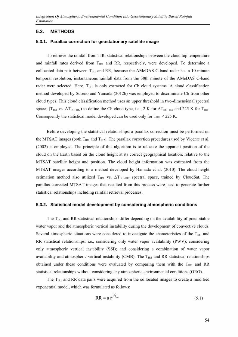
Integration Of Atmospheric Environmental Condition Into Geostationary Satellite Based Rainfall Estimation
54
5.3. METHODS
5.3.1. Parallax correction for geostationary satellite image
To retrieve the rainfall from TIR, statistical relationships between the cloud top temperature
and rainfall rates derived from TIR1 and RR, respectively, were developed. To determine a
collocated data pair between TIR1 and RR, because the AMeDAS C-band radar has a 10-minute
temporal resolution, instantaneous rainfall data from the 30th minute of the AMeDAS C-band
radar were selected. Here, TIR1 is only extracted for Cb cloud systems. A cloud classification
method developed by Suseno and Yamada (2012b) was employed to discriminate Cb from other
cloud types. This cloud classification method uses an upper threshold in two-dimensional spectral
spaces (TIR1 vs. ΔTIR1–IR2) to define the Cb cloud type, i.e., 2 K for ΔTIR1–IR2 and 225 K for TIR1.
Consequently the statistical model developed can be used only for TIR1 < 225 K.
Before developing the statistical relationships, a parallax correction must be performed on
the MTSAT images (both TIR1 and TIR2). The parallax correction procedures used by Vicente et al.
(2002) is employed. The principle of this algorithm is to relocate the apparent position of the
cloud on the Earth based on the cloud height at its correct geographical location, relative to the
MTSAT satellite height and position. The cloud height information was estimated from the
MTSAT images according to a method developed by Hamada et al. (2010). The cloud height
estimation method also utilized TIR1 vs. ΔTIR1–IR2 spectral space, trained by CloudSat. The
parallax-corrected MTSAT images that resulted from this process were used to generate further
statistical relationships including rainfall retrieval processes.
5.3.2. Statistical model development by considering atmospheric conditions
The TIR1 and RR statistical relationships differ depending on the availability of precipitable
water vapor and the atmospheric vertical instability during the development of convective clouds.
Several atmospheric situations were considered to investigate the characteristics of the TIR1 and
RR statistical relationships: i.e., considering only water vapor availability (PWV); considering
only atmospheric vertical instability (SSI); and considering a combination of water vapor
availability and atmospheric vertical instability (CMB). The TIR1 and RR statistical relationships
obtained under these conditions were evaluated by comparing them with the TIR1 and RR
statistical relationships without considering any atmospheric environmental conditions (ORG).
The TIR1 and RR data pairs were acquired from the collocated images to create a modified
exponential model, which was formulated as follows:
IR1Tb
eaRR = (5.1)
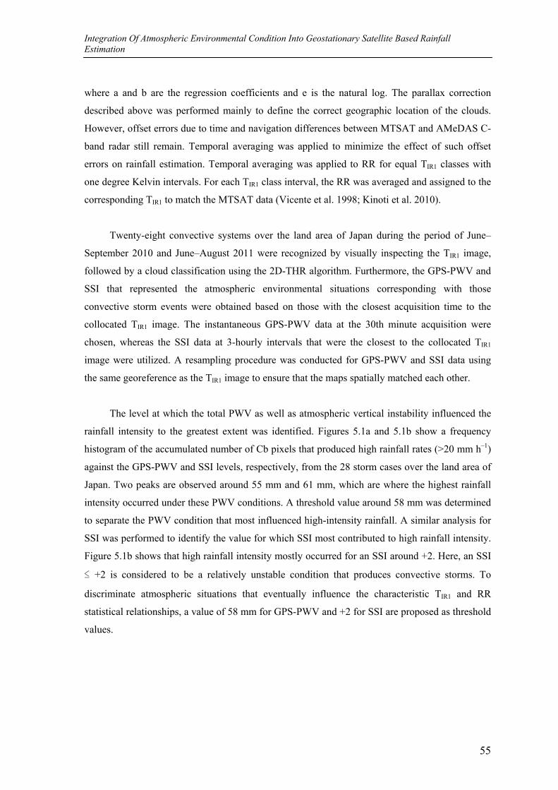
Integration Of Atmospheric Environmental Condition Into Geostationary Satellite Based Rainfall Estimation
55
where a and b are the regression coefficients and e is the natural log. The parallax correction
described above was performed mainly to define the correct geographic location of the clouds.
However, offset errors due to time and navigation differences between MTSAT and AMeDAS C-
band radar still remain. Temporal averaging was applied to minimize the effect of such offset
errors on rainfall estimation. Temporal averaging was applied to RR for equal TIR1 classes with
one degree Kelvin intervals. For each TIR1 class interval, the RR was averaged and assigned to the
corresponding TIR1 to match the MTSAT data (Vicente et al. 1998; Kinoti et al. 2010).
Twenty-eight convective systems over the land area of Japan during the period of June–
September 2010 and June–August 2011 were recognized by visually inspecting the TIR1 image,
followed by a cloud classification using the 2D-THR algorithm. Furthermore, the GPS-PWV and
SSI that represented the atmospheric environmental situations corresponding with those
convective storm events were obtained based on those with the closest acquisition time to the
collocated TIR1 image. The instantaneous GPS-PWV data at the 30th minute acquisition were
chosen, whereas the SSI data at 3-hourly intervals that were the closest to the collocated TIR1
image were utilized. A resampling procedure was conducted for GPS-PWV and SSI data using
the same georeference as the TIR1 image to ensure that the maps spatially matched each other.
The level at which the total PWV as well as atmospheric vertical instability influenced the
rainfall intensity to the greatest extent was identified. Figures 5.1a and 5.1b show a frequency
histogram of the accumulated number of Cb pixels that produced high rainfall rates (>20 mm h–1)
against the GPS-PWV and SSI levels, respectively, from the 28 storm cases over the land area of
Japan. Two peaks are observed around 55 mm and 61 mm, which are where the highest rainfall
intensity occurred under these PWV conditions. A threshold value around 58 mm was determined
to separate the PWV condition that most influenced high-intensity rainfall. A similar analysis for
SSI was performed to identify the value for which SSI most contributed to high rainfall intensity.
Figure 5.1b shows that high rainfall intensity mostly occurred for an SSI around +2. Here, an SSI
≤ +2 is considered to be a relatively unstable condition that produces convective storms. To
discriminate atmospheric situations that eventually influence the characteristic TIR1 and RR
statistical relationships, a value of 58 mm for GPS-PWV and +2 for SSI are proposed as threshold
values.
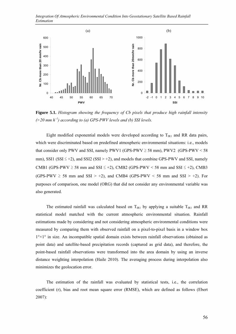
Integration Of Atmospheric Environmental Condition Into Geostationary Satellite Based Rainfall Estimation
56
(a) (b)
0
100
200
300
400
500
600
40 45 50 55 60 65 70
PWV
Nr.
Cb
mor
e th
an 2
0 m
m/h
r rai
n
0
200
400
600
800
1000
-2 -1 0 1 2 3 4 5 6 7 8 9 10
SSI
Nr.
Cb
mor
e th
an 2
0mm
/hr r
ain
Figure 5.1. Histogram showing the frequency of Cb pixels that produce high rainfall intensity
(>20 mm h–1) according to (a) GPS-PWV levels and (b) SSI levels.
Eight modified exponential models were developed according to TIR1 and RR data pairs,
which were discriminated based on predefined atmospheric environmental situations: i.e., models
that consider only PWV and SSI, namely PWV1 (GPS-PWV ≥ 58 mm), PWV2 (GPS-PWV < 58
mm), SSI1 (SSI ≤ +2), and SSI2 (SSI > +2), and models that combine GPS-PWV and SSI, namely
CMB1 (GPS-PWV ≥ 58 mm and SSI ≤ +2), CMB2 (GPS-PWV < 58 mm and SSI ≤ +2), CMB3
(GPS-PWV ≥ 58 mm and SSI > +2), and CMB4 (GPS-PWV < 58 mm and SSI > +2). For
purposes of comparison, one model (ORG) that did not consider any environmental variable was
also generated.
The estimated rainfall was calculated based on TIR1 by applying a suitable TIR1 and RR
statistical model matched with the current atmospheric environmental situation. Rainfall
estimations made by considering and not considering atmospheric environmental conditions were
measured by comparing them with observed rainfall on a pixel-to-pixel basis in a window box
1°×1° in size. An incompatible spatial domain exists between rainfall observations (obtained as
point data) and satellite-based precipitation records (captured as grid data), and therefore, the
point-based rainfall observations were transformed into the area domain by using an inverse
distance weighting interpolation (Haile 2010). The averaging process during interpolation also
minimizes the geolocation error.
The estimation of the rainfall was evaluated by statistical tests, i.e., the correlation
coefficient (r), bias and root mean square error (RMSE), which are defined as follows (Ebert
2007):
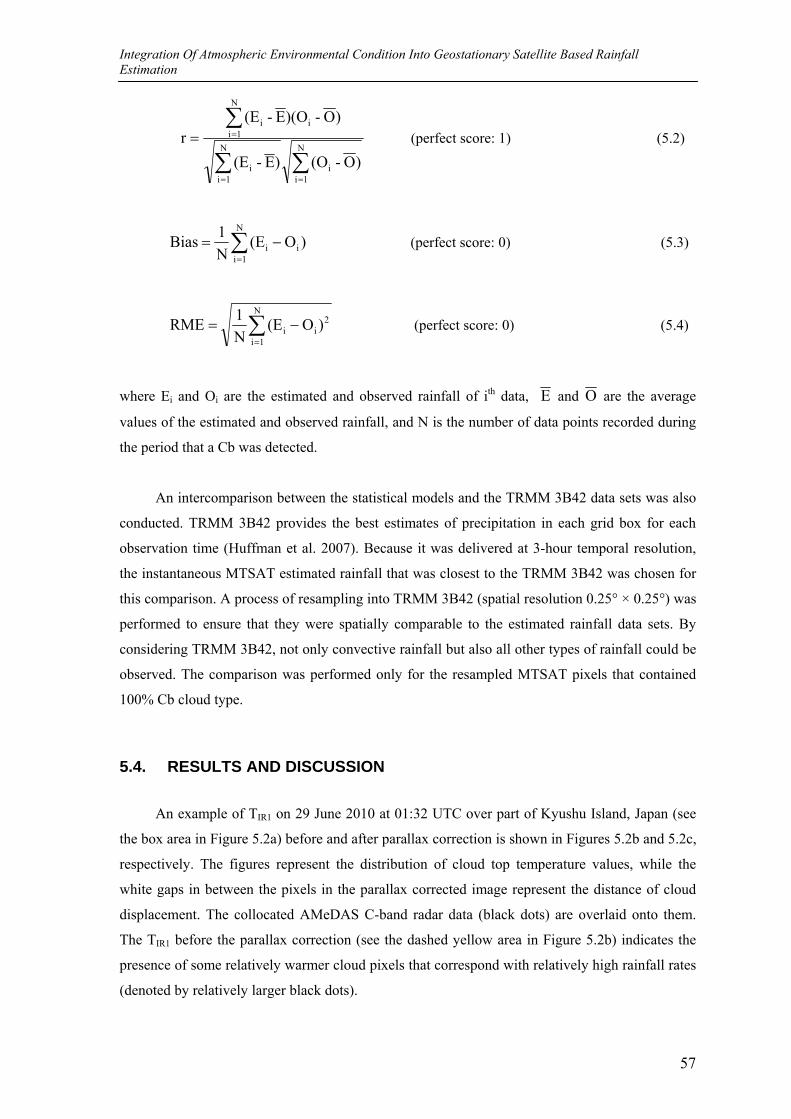
Integration Of Atmospheric Environmental Condition Into Geostationary Satellite Based Rainfall Estimation
57
∑∑
∑
==
==N
1ii
N
1ii
N
1iii
)O-(O)E-(E
)O-)(OE-(Er (perfect score: 1) (5.2)
∑=
−=N
1iii )O(E
N1Bias (perfect score: 0) (5.3)
∑=
−=N
1i
2ii )O(E
N1RME (perfect score: 0) (5.4)
where Ei and Oi are the estimated and observed rainfall of ith data, E and O are the average
values of the estimated and observed rainfall, and N is the number of data points recorded during
the period that a Cb was detected.
An intercomparison between the statistical models and the TRMM 3B42 data sets was also
conducted. TRMM 3B42 provides the best estimates of precipitation in each grid box for each
observation time (Huffman et al. 2007). Because it was delivered at 3-hour temporal resolution,
the instantaneous MTSAT estimated rainfall that was closest to the TRMM 3B42 was chosen for
this comparison. A process of resampling into TRMM 3B42 (spatial resolution 0.25° × 0.25°) was
performed to ensure that they were spatially comparable to the estimated rainfall data sets. By
considering TRMM 3B42, not only convective rainfall but also all other types of rainfall could be
observed. The comparison was performed only for the resampled MTSAT pixels that contained
100% Cb cloud type.
5.4. RESULTS AND DISCUSSION
An example of TIR1 on 29 June 2010 at 01:32 UTC over part of Kyushu Island, Japan (see
the box area in Figure 5.2a) before and after parallax correction is shown in Figures 5.2b and 5.2c,
respectively. The figures represent the distribution of cloud top temperature values, while the
white gaps in between the pixels in the parallax corrected image represent the distance of cloud
displacement. The collocated AMeDAS C-band radar data (black dots) are overlaid onto them.
The TIR1 before the parallax correction (see the dashed yellow area in Figure 5.2b) indicates the
presence of some relatively warmer cloud pixels that correspond with relatively high rainfall rates
(denoted by relatively larger black dots).
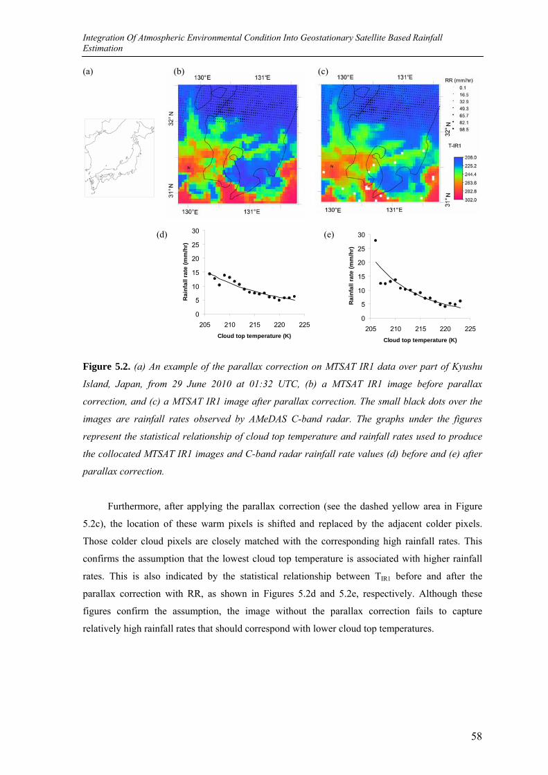
Integration Of Atmospheric Environmental Condition Into Geostationary Satellite Based Rainfall Estimation
58
0
5
10
15
20
25
30
205 210 215 220 225Cloud top temperature (K)
Rai
nfal
l rat
e (m
m/h
r)
0
5
10
15
20
25
30
205 210 215 220 225Cloud top temperature (K)
Rai
nfal
l rat
e (m
m/h
r)
(a) (b) (c)
(d) (e)
Figure 5.2. (a) An example of the parallax correction on MTSAT IR1 data over part of Kyushu
Island, Japan, from 29 June 2010 at 01:32 UTC, (b) a MTSAT IR1 image before parallax
correction, and (c) a MTSAT IR1 image after parallax correction. The small black dots over the
images are rainfall rates observed by AMeDAS C-band radar. The graphs under the figures
represent the statistical relationship of cloud top temperature and rainfall rates used to produce
the collocated MTSAT IR1 images and C-band radar rainfall rate values (d) before and (e) after
parallax correction.
Furthermore, after applying the parallax correction (see the dashed yellow area in Figure
5.2c), the location of these warm pixels is shifted and replaced by the adjacent colder pixels.
Those colder cloud pixels are closely matched with the corresponding high rainfall rates. This
confirms the assumption that the lowest cloud top temperature is associated with higher rainfall
rates. This is also indicated by the statistical relationship between TIR1 before and after the
parallax correction with RR, as shown in Figures 5.2d and 5.2e, respectively. Although these
figures confirm the assumption, the image without the parallax correction fails to capture
relatively high rainfall rates that should correspond with lower cloud top temperatures.
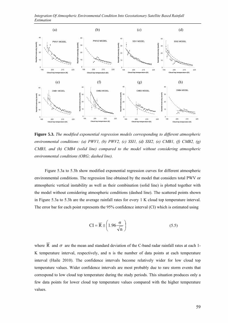
Integration Of Atmospheric Environmental Condition Into Geostationary Satellite Based Rainfall Estimation
59
(a) (b) (c) (d)
0
10
20
30
40
195 205 215 225
Cloud top temperature (K)
Rai
nfal
l ins
tens
ity (m
m/h
) PWV1 MODEL
0
10
20
30
40
195 205 215 225
Cloud top temperature (K)
Rai
nfal
l ins
tens
ity (m
m/h
)
PWV2 MODEL
0
10
20
30
40
195 205 215 225Cloud top temperature (K)
Rai
nfal
l ins
tens
ity (m
m/h
)
SSI1 MODEL
0
10
20
30
40
195 205 215 225Cloud top temperature (K)
Rai
nfal
l ins
tens
ity (m
m/h
)
SSI2 MODEL
(e) (f) (g) (h)
0
10
20
30
40
195 205 215 225Cloud top temperature (K)
Rai
nfal
l ins
tens
ity (m
m/h
)
CMB1 MODEL
0
10
20
30
40
195 205 215 225
Cloud top temperature (K)
Rai
nfal
l ins
tens
ity (m
m/h
)
CMB2 MODEL
0
10
20
30
40
195 205 215 225Cloud top temperature (K)
Rai
nfal
l ins
tens
ity (m
m/h
)
CMB3 MODEL
0
10
20
30
40
195 205 215 225
Cloud top temperature (K)
Rai
nfal
l ins
tens
ity (m
m/h
)
CMB4 MODEL
Figure 5.3. The modified exponential regression models corresponding to different atmospheric
environmental conditions: (a) PWV1, (b) PWV2, (c) SSI1, (d) SSI2, (e) CMB1, (f) CMB2, (g)
CMB3, and (h) CMB4 (solid line) compared to the model without considering atmospheric
environmental conditions (ORG; dashed line).
Figure 5.3a to 5.3h show modified exponential regression curves for different atmospheric
environmental conditions. The regression line obtained by the model that considers total PWV or
atmospheric vertical instability as well as their combination (solid line) is plotted together with
the model without considering atmospheric conditions (dashed line). The scattered points shown
in Figure 5.3a to 5.3h are the average rainfall rates for every 1 K cloud top temperature interval.
The error bar for each point represents the 95% confidence interval (CI) which is estimated using
⎟⎠⎞
⎜⎝⎛±=
nσ1.96RCI (5.5)
where R and σ are the mean and standard deviation of the C-band radar rainfall rates at each 1-
K temperature interval, respectively, and n is the number of data points at each temperature
interval (Haile 2010). The confidence intervals become relatively wider for low cloud top
temperature values. Wider confidence intervals are most probably due to rare storm events that
correspond to low cloud top temperature during the study periods. This situation produces only a
few data points for lower cloud top temperature values compared with the higher temperature
values.
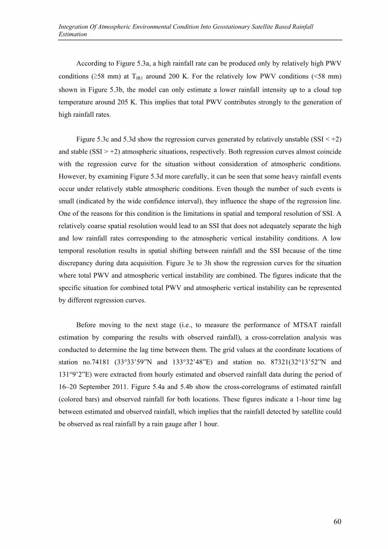
Integration Of Atmospheric Environmental Condition Into Geostationary Satellite Based Rainfall Estimation
60
According to Figure 5.3a, a high rainfall rate can be produced only by relatively high PWV
conditions (≥58 mm) at TIR1 around 200 K. For the relatively low PWV conditions (<58 mm)
shown in Figure 5.3b, the model can only estimate a lower rainfall intensity up to a cloud top
temperature around 205 K. This implies that total PWV contributes strongly to the generation of
high rainfall rates.
Figure 5.3c and 5.3d show the regression curves generated by relatively unstable (SSI < +2)
and stable (SSI > +2) atmospheric situations, respectively. Both regression curves almost coincide
with the regression curve for the situation without consideration of atmospheric conditions.
However, by examining Figure 5.3d more carefully, it can be seen that some heavy rainfall events
occur under relatively stable atmospheric conditions. Even though the number of such events is
small (indicated by the wide confidence interval), they influence the shape of the regression line.
One of the reasons for this condition is the limitations in spatial and temporal resolution of SSI. A
relatively coarse spatial resolution would lead to an SSI that does not adequately separate the high
and low rainfall rates corresponding to the atmospheric vertical instability conditions. A low
temporal resolution results in spatial shifting between rainfall and the SSI because of the time
discrepancy during data acquisition. Figure 3e to 3h show the regression curves for the situation
where total PWV and atmospheric vertical instability are combined. The figures indicate that the
specific situation for combined total PWV and atmospheric vertical instability can be represented
by different regression curves.
Before moving to the next stage (i.e., to measure the performance of MTSAT rainfall
estimation by comparing the results with observed rainfall), a cross-correlation analysis was
conducted to determine the lag time between them. The grid values at the coordinate locations of
station no.74181 (33°33’59”N and 133°32’48”E) and station no. 87321(32°13’52”N and
131°9’2”E) were extracted from hourly estimated and observed rainfall data during the period of
16–20 September 2011. Figure 5.4a and 5.4b show the cross-correlograms of estimated rainfall
(colored bars) and observed rainfall for both locations. These figures indicate a 1-hour time lag
between estimated and observed rainfall, which implies that the rainfall detected by satellite could
be observed as real rainfall by a rain gauge after 1 hour.
Integration Of Atmospheric Environmental Condition Into Geostationary Satellite Based Rainfall Estimation
61
(a) (b)
-0.1
0
0.1
0.2
0.3
0.4
0.5
0.6
0.7
-10 -8 -6 -4 -2 0 2 4 6 8 10
Lag (hour)
Cro
ss C
orre
latio
n
CMB PWV SSI ORG
0
0.1
0.2
0.3
0.4
0.5
0.6
0.7
0.8
-10 -8 -6 -4 -2 0 2 4 6 8 10
Lag (hour)
Cro
ss C
orre
latio
n
CMB PWV SSI ORG Figure 5.4. Cross-correlograms of estimated and observed rainfall for (a) station no. 74181 and
(b) station no. 87321. In both cases, the maximum correlation occurs at a time lag of negative 1-
hour.
The performance of the statistical models was tested in three case studies: (1) 22 June 2010
at 06:30–13:30 UTC over Kyushu Island (beginning of summer; hereinafter case A); (2) 24
August 2011 at 15:32–21:32 UTC over Nara Prefecture (middle of summer; hereinafter case B);
and (3) 19–20 September 2011 at 17:32–05:32 UTC over Kyushu Island (end of summer;
hereinafter case C). The locations of these three case studies are shown in Figure 5.5a.
To show the difference among statistical models, a snapshot of the rainfall during the peak
of a heavy rainfall event on 22 June 2010 at 11:30 UTC over Kyushu Island Japan (case A) was
estimated using the model without consideration of any atmospheric conditions (Figure 5.5b), the
model considering only PWV (Figure 5.5c), the model considering only SSI (Figure 5.5d), and
the model considering both PWV and SSI (Figure 5.5e). As explained above, there was a 1-hour
time lag between estimated rainfall and observed rainfall; therefore, the estimated rainfall results
were compared with interpolated observed rainfall (Figure 5.5f) for the following hour (i.e., 12:30
UTC). Compared with the observed rainfall, MTSAT rainfall estimations did not represent local
strong rainfall events very well, even though in the wider spatial domain, they provided a
reasonable representation of the spatial distribution of rainfall.
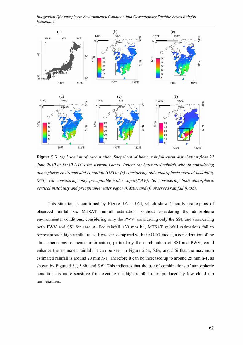
Integration Of Atmospheric Environmental Condition Into Geostationary Satellite Based Rainfall Estimation
62
(a) (b) (c)
(d) (e) (f)
Figure 5.5. (a) Location of case studies. Snapshoot of heavy rainfall event distribution from 22
June 2010 at 11:30 UTC over Kyushu Island, Japan; (b) Estimated rainfall without considering
atmospheric environmental condition (ORG); (c) considering only atmospheric vertical instability
(SSI); (d) considering only precipitable water vapor(PWV); (e) considering both atmospheric
vertical instability and precipitable water vapor (CMB); and (f) observed rainfall (OBS).
This situation is confirmed by Figure 5.6a– 5.6d, which show 1-hourly scatterplots of
observed rainfall vs. MTSAT rainfall estimations without considering the atmospheric
environmental conditions, considering only the PWV, considering only the SSI, and considering
both PWV and SSI for case A. For rainfall >30 mm h-1, MTSAT rainfall estimations fail to
represent such high rainfall rates. However, compared with the ORG model, a consideration of the
atmospheric environmental information, particularly the combination of SSI and PWV, could
enhance the estimated rainfall. It can be seen in Figure 5.6a, 5.6e, and 5.6i that the maximum
estimated rainfall is around 20 mm h-1. Therefore it can be increased up to around 25 mm h-1, as
shown by Figure 5.6d, 5.6h, and 5.6l. This indicates that the use of combinations of atmospheric
conditions is more sensitive for detecting the high rainfall rates produced by low cloud top
temperatures.
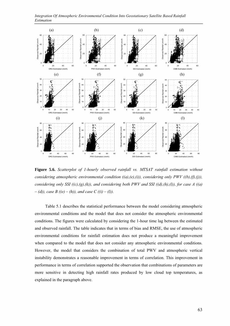
Integration Of Atmospheric Environmental Condition Into Geostationary Satellite Based Rainfall Estimation
63
(a) (b) (c) (d)
0
20
40
60
0 20 40 60
ORG Estimated (mm/h)
Obs
erve
d R
ainf
all (
mm
/h
0
20
40
60
0 20 40 60
PWV Estimated (mm/h)
Obs
erve
d R
ainf
all (
mm
/h
0
20
40
60
0 20 40 60
SSI Estimated (mm/h)
Obs
erve
d R
ainf
all (
mm
/h
0
20
40
60
0 20 40 60
CMB Estimated (mm/h)
Obs
erve
d R
ainf
all (
mm
/h
(e) (f) (g) (h)
0
10
20
30
40
50
0 10 20 30 40 50
ORG Estimated (mm/h)
Obs
erve
d R
ainf
all (
mm
/h
0
10
20
30
40
50
0 10 20 30 40 50
PWV Estimated (mm/h)
Obs
erve
d R
ainf
all (
mm
/h
0
10
20
30
40
50
0 10 20 30 40 50
SSI Estimated (mm/h)
Obs
erve
d R
ainf
all (
mm
/h
0
10
20
30
40
50
0 10 20 30 40 50
CMB Estimated (mm/h)
Obs
erve
d R
ainf
all (
mm
/h
(i) (j) (k) (l)
0
20
40
60
80
0 20 40 60 80
ORG Estimated (mm/h)
Obs
erve
d R
ainf
all (
mm
/h
0
20
40
60
80
0 20 40 60 80
PWV Estimated (mm/h)
Obs
erve
d R
ainf
all (
mm
/h
0
20
40
60
80
0 20 40 60 80
SSI Estimated (mm/h)
Obs
erve
d R
ainf
all (
mm
/h
0
20
40
60
80
0 20 40 60 80
CMB Estimated (mm/h)
Obs
erve
d R
ainf
all (
mm
/h
Figure 5.6. Scatterplot of 1-hourly observed rainfall vs. MTSAT rainfall estimation without
considering atmospheric environmental condition ((a),(e),(i)), considering only PWV ((b),(f),(j)),
considering only SSI ((c),(g),(k)), and considering both PWV and SSI ((d),(h),(l)), for case A ((a)
– (d)), case B ((e) – (h)), and case C ((i) – (l)).
Table 5.1 describes the statistical performance between the model considering atmospheric
environmental conditions and the model that does not consider the atmospheric environmental
conditions. The figures were calculated by considering the 1-hour time lag between the estimated
and observed rainfall. The table indicates that in terms of bias and RMSE, the use of atmospheric
environmental conditions for rainfall estimation does not produce a meaningful improvement
when compared to the model that does not consider any atmospheric environmental conditions.
However, the model that considers the combination of total PWV and atmospheric vertical
instability demonstrates a reasonable improvement in terms of correlation. This improvement in
performance in terms of correlation supported the observation that combinations of parameters are
more sensitive in detecting high rainfall rates produced by low cloud top temperatures, as
explained in the paragraph above.
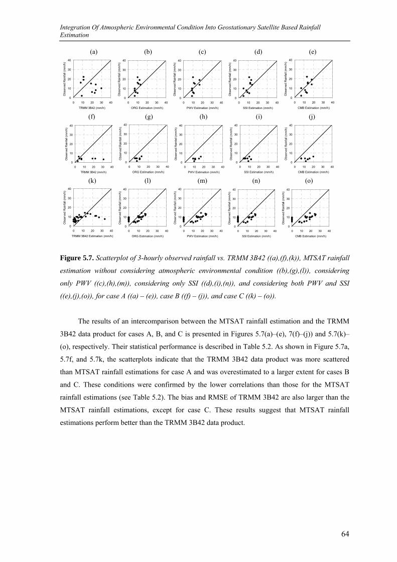
Integration Of Atmospheric Environmental Condition Into Geostationary Satellite Based Rainfall Estimation
64
(a) (b) (c) (d) (e)
0
10
20
30
40
0 10 20 30 40
TRMM 3B42 (mm/h)
Obs
erve
d R
ainf
all (
mm
/h)
0
10
20
30
40
0 10 20 30 40
ORG Estimation (mm/h)
Obs
erve
d R
ainf
all (
mm
/h)
0
10
20
30
40
0 10 20 30 40
PWV Estimation (mm/h)
Obs
erve
d R
ainf
all (
mm
/h)
0
10
20
30
40
0 10 20 30 40
SSI Estimation (mm/h)
Obs
erve
d R
ainf
all (
mm
/h)
0
10
20
30
40
0 10 20 30 40
CMB Estimation (mm/h)
Obs
erve
d R
ainf
all (
mm
/h)
(f) (g) (h) (i) (j)
0
10
20
30
40
0 10 20 30 40
TRMM 3B42 (mm/h)
Obs
erve
d R
ainf
all (
mm
/h)
0
10
20
30
40
0 10 20 30 40
ORG Estimation (mm/h)
Obs
erve
d R
ainf
all (
mm
/h)
0
10
20
30
40
0 10 20 30 40
PWV Estimation (mm/h)O
bser
ved
Rai
nfal
l (m
m/h
)
0
10
20
30
40
0 10 20 30 40
SSI Estimation (mm/h)
Obs
erve
d R
ainf
all (
mm
/h)
0
10
20
30
40
0 10 20 30 40
CMB Estimation (mm/h)
Obs
erve
d R
ainf
all (
mm
/h)
(k) (l) (m) (n) (o)
0
10
20
30
40
0 10 20 30 40
TRMM 3B42 Estimation (mm/h)
Obs
erve
d R
ainf
all (
mm
/h)
0
10
20
30
40
0 10 20 30 40
ORG Estimation (mm/h)
Obs
erve
d R
ainf
all (
mm
/h)
0
10
20
30
40
0 10 20 30 40
PWV Estimation (mm/h)
Obs
erve
d R
ainf
all (
mm
/h)
0
10
20
30
40
0 10 20 30 40
SSI Estimation (mm/h)
Obs
erve
d R
ainf
all (
mm
/h)
0
10
20
30
40
0 10 20 30 40
CMB Estimation (mm/h)
Obs
erve
d R
ainf
all (
mm
/h)
Figure 5.7. Scatterplot of 3-hourly observed rainfall vs. TRMM 3B42 ((a),(f),(k)), MTSAT rainfall
estimation without considering atmospheric environmental condition ((b),(g),(l)), considering
only PWV ((c),(h),(m)), considering only SSI ((d),(i),(n)), and considering both PWV and SSI
((e),(j),(o)), for case A ((a) – (e)), case B ((f) – (j)), and case C ((k) – (o)).
The results of an intercomparison between the MTSAT rainfall estimation and the TRMM
3B42 data product for cases A, B, and C is presented in Figures 5.7(a)–(e), 7(f)–(j)) and 5.7(k)–
(o), respectively. Their statistical performance is described in Table 5.2. As shown in Figure 5.7a,
5.7f, and 5.7k, the scatterplots indicate that the TRMM 3B42 data product was more scattered
than MTSAT rainfall estimations for case A and was overestimated to a larger extent for cases B
and C. These conditions were confirmed by the lower correlations than those for the MTSAT
rainfall estimations (see Table 5.2). The bias and RMSE of TRMM 3B42 are also larger than the
MTSAT rainfall estimations, except for case C. These results suggest that MTSAT rainfall
estimations perform better than the TRMM 3B42 data product.
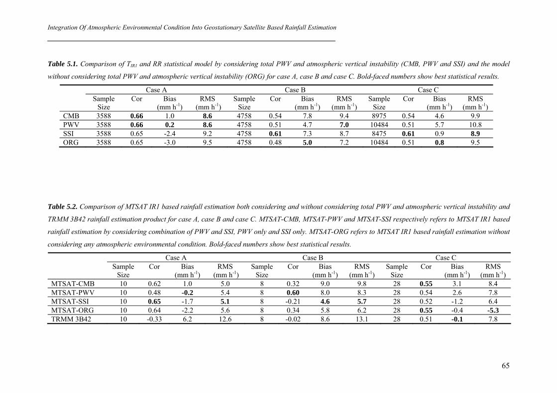
Integration Of Atmospheric Environmental Condition Into Geostationary Satellite Based Rainfall Estimation
65
Table 5.1. Comparison of TIR1 and RR statistical model by considering total PWV and atmospheric vertical instability (CMB, PWV and SSI) and the model
without considering total PWV and atmospheric vertical instability (ORG) for case A, case B and case C. Bold-faced numbers show best statistical results.
Case A Case B Case C Sample
Size Cor Bias
(mm h-1) RMS
(mm h-1) Sample
Size Cor Bias
(mm h-1) RMS
(mm h-1) Sample
Size Cor Bias
(mm h-1) RMS
(mm h-1) CMB 3588 0.66 1.0 8.6 4758 0.54 7.8 9.4 8975 0.54 4.6 9.9 PWV 3588 0.66 0.2 8.6 4758 0.51 4.7 7.0 10484 0.51 5.7 10.8 SSI 3588 0.65 -2.4 9.2 4758 0.61 7.3 8.7 8475 0.61 0.9 8.9 ORG 3588 0.65 -3.0 9.5 4758 0.48 5.0 7.2 10484 0.51 0.8 9.5
Table 5.2. Comparison of MTSAT IR1 based rainfall estimation both considering and without considering total PWV and atmospheric vertical instability and
TRMM 3B42 rainfall estimation product for case A, case B and case C. MTSAT-CMB, MTSAT-PWV and MTSAT-SSI respectively refers to MTSAT IR1 based
rainfall estimation by considering combination of PWV and SSI, PWV only and SSI only. MTSAT-ORG refers to MTSAT IR1 based rainfall estimation without
considering any atmospheric environmental condition. Bold-faced numbers show best statistical results.
Case A Case B Case C Sample
Size Cor Bias
(mm h-1) RMS
(mm h-1) Sample
Size Cor Bias
(mm h-1) RMS
(mm h-1) Sample
Size Cor Bias
(mm h-1) RMS
(mm h-1) MTSAT-CMB 10 0.62 1.0 5.0 8 0.32 9.0 9.8 28 0.55 3.1 8.4 MTSAT-PWV 10 0.48 -0.2 5.4 8 0.60 8.0 8.3 28 0.54 2.6 7.8 MTSAT-SSI 10 0.65 -1.7 5.1 8 -0.21 4.6 5.7 28 0.52 -1.2 6.4 MTSAT-ORG 10 0.64 -2.2 5.6 8 0.34 5.8 6.2 28 0.55 -0.4 -5.3 TRMM 3B42 10 -0.33 6.2 12.6 8 -0.02 8.6 13.1 28 0.51 -0.1 7.8
Integration Of Atmospheric Environmental Condition Into Geostationary Satellite Based Rainfall Estimation
66
5.5. SUMMARY AND CONCLUSIONS
A method of rainfall estimation based on the statistical relationships between TIR1 and RR
was developed for heavy rainfall generated by convective cloud in Japan and the surrounding area.
TIR1 and RR data were acquired from MTSAT IR1 and AMeDAS C-band radar, respectively, for
the periods of June–September 2010 and 2011. A parallax error correction was performed for the
MTSAT data sets. To differentiate between convective and non-convective cloud, the 2D-THR
cloud classification algorithm was applied to the parallax-corrected MTSAT data sets. The total
PWV and atmospheric vertical instability conditions during the convection process, which
influence the TIR1 and RR statistical relationships, were investigated. These atmospheric
environmental conditions were represented by GPS-PWV and SSI, respectively. Values of 58 mm
for GPS-PWV and +2 for SSI were proposed as thresholds for discriminating such atmospheric
environmental conditions. Eight modified exponential models were developed according to TIR1
and RR data pairs, which were discriminated based on predefined atmospheric environmental
situations: i.e., models that considered only PWV and SSI, namely PWV1 (GPS-PWV ≥ 58 mm),
PWV2 (GPS-PWV < 58 mm), SSI1 (SSI ≤ +2), and SSI2 (SSI > +2), and models that combined
GPS-PWV and SSI, namely CMB1 (GPS-PWV ≥ 58 mm and SSI ≤ +2), CMB2 (GPS-PWV < 58
mm and SSI ≤ +2), CMB3 (GPS-PWV ≥ 58 mm and SSI > +2), and CMB4 (GPS-PWV < 58 mm
and SSI > +2). One model, namely ORG, which did not consider GPS-PWV and SSI, was also
generated.
Several different regression curves for the statistical relationships of TIR1 and RR were
produced, especially by combining PWV and SSI conditions. Due to the occurrence of rare storm
events that corresponded to low cloud top temperatures during this study period, the confidence
intervals of the statistical model became relatively wider for low cloud top temperature values.
Based on those regression curves the rainfall estimation is conducted based on cloud top
temperature by considering specific atmospheric environmental conditions.
When compared with the model that did not consider any atmospheric environmental
conditions, the use of atmospheric environmental conditions for making rainfall estimations
enhanced the accuracy of rainfall estimation, particularly when using the model that considered a
combination of total PWV and atmospheric vertical instability, and eventually improved the
performance, particularly in terms of correlation. However MTSAT rainfall estimation was not
successful in representing local heavy rainfall events, even though it performed reasonably well
when predicting the rainfall spatial distribution at a wider spatial domain.

Integration Of Atmospheric Environmental Condition Into Geostationary Satellite Based Rainfall Estimation
67
The intercomparison results between MTSAT IR1-based rainfall estimations and the
TRMM 3B42 data product demonstrated that MTSAT IR1-based rainfall estimations either
considering or not considering total PWV and atmospheric vertical instability, produced a
reasonably better performance than the TRMM 3B42 data product.
Because of the limitation of the number of samples that were used in this study, the
full variety of physical processes associated with convective rainfall generation may not
have been included. Therefore, more samples should be included in the development and
validation of statistical models to reach a more definite conclusion.
Chapter 6. EMPIRICAL REGRESSION BASED RAINFALL-RUNOFF MODEL FOR FLASH FLOODS SEVERITY ASSESSMENT
Prepared for publication
Statistical analysis for flash floods severity assessment
69
Abstract
Flash floods are one of the most dangerous hazards that are difficult to forecast. Therefore,
identification of flash flood prone catchments is important for their risk reduction and mitigation.
The catchments that potential in producing flash floods are represented by their relative flash
flood severity. Flash floods are considered severe when they have relative high magnitude and
high rising hydrograph gradient. This study intends to use some hydrological, morphometrical and
meteorological factors to characterize flash flood severity and develop some empirical models to
draw the relationship among them. 16 gauged sub-catchments in western Hokkaido region have
been delineated. The highest discharge within June to October in each year that has time to peak
discharge less than 12 hours is identified and selected as the flash flood event during the period of
1998 – 2009. The flash floods severity is analyzed for each sub-catchments based on hydrograph
analysis. The hydrological, morphometrical and meteorological condition of those catchments are
identified. The step-wise multiple regression analysis demonstrates that the land use contributing
area is dominant factor related to flash flood severity in Ishikari river basin, particularly under
initially wet soil moisture condition. For the morphometrical parameters the prominent parameters
are those related to basin shape (i.e. elongation ratio) and topography (i.e. relief ratio and melton’s
ruggedness number). For the meteorological parameter, the rainfall intensity is utilized to assess
the flash flood severity. The implementation of the empirical models at Toyohira basin shows that
FI as the function of morphometrical factors can provide flash flood potential information.
Moreover, FI as the function of hydrological and meteorological factors demonstrate more
dynamic pattern since they are related to rainfall intensity distribution.
Key Words: Flash flood, severity index, multiple regression analysis

Statistical analysis for flash floods severity assessment
70
6.1. INTRODUCTION
The sudden and destructive nature of flash floods make they considered as one of the most
dangerous hazards. The flash floods, when compared to normal floods are characterized by quite
rapid rises and falls with little or no advance warning. These types of floods are resulted from
very intense rainfall over a relatively small area (NRC, 2005). Flash floods are also difficult to
forecast because the task is not only to forecast the occurrence of the events but also their
magnitude should be anticipated (Doswell et al., 1996).
Several efforts to reduce the flash floods risk is by identifying the potential of flash floods
occurrence in particular ungauged catchments have been performed by some researchers. Yousef
et al. (2010) was conducting a morphometrical analysis to estimate flash flood risk levels in an
arid environment. Angilierri (2010) also analyze various morphometrical characteristic over some
catchments area in order to evaluate flash flood hazard. Both studies have made use some sources
of spatial data which are mainly derived from topographic map and satellite imagery to identify
the morphological features. The results of those studies show that they can initiate appropriate
measures to mitigate the potential hazard in the area.
In this study, flash floods is considered as the output of a catchment system that are
determined by not only by hydraulic processes related to the morphology of stream but also
meteorological and hydrological factor such as slope, land use, geology (NRC, 2005). The flash
floods are mostly triggered by severe convective storm that typically developed under unstable
atmospheric condition, modulated by the hydrological condition and sometimes amplified by the
catchment’s morphology and network structure. Because flash floods are resulted as the response
of the catchments to the rainfall that is controlled by the hydrological and morphologic factors,
thus they can be used as the proxies to determined flash flood hazard potential.
Beven and Kirkby (1979) mentioned that for the humid and temperate basin, the runoff
generation mechanism is mainly influenced by: (i) rainfall intensity that exceed infiltration or
storage capacity on a variable area; and (ii) rainfall that directly fall in channel and completely
saturated soil. In this study the variable area that contributes to runoff is assumed to influence the
flash flood severity index. A combined various land surface condition (i.e. land use, surface
permeability and slope steepness) and rainfall intensity in a catchment is considered as variable
contributing area. The soil saturation condition is identified according to initial soil moisture
condition by using simple water balance calculation.
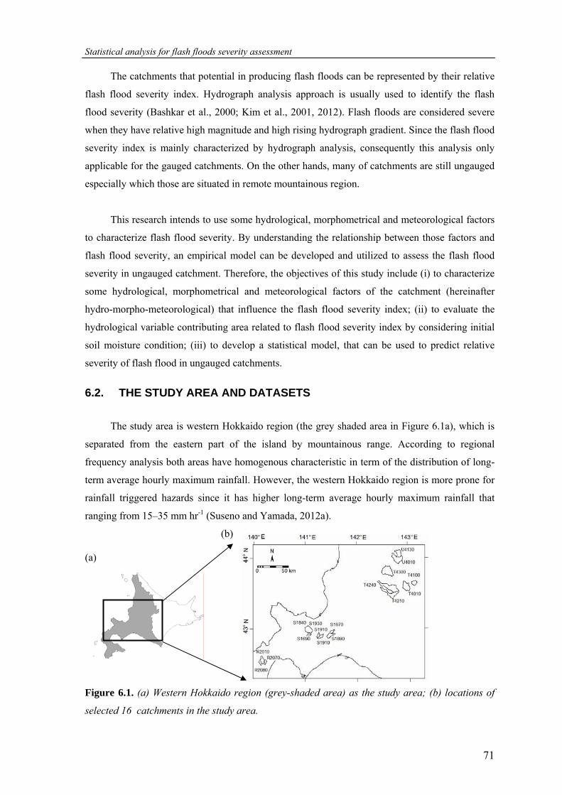
Statistical analysis for flash floods severity assessment
71
The catchments that potential in producing flash floods can be represented by their relative
flash flood severity index. Hydrograph analysis approach is usually used to identify the flash
flood severity (Bashkar et al., 2000; Kim et al., 2001, 2012). Flash floods are considered severe
when they have relative high magnitude and high rising hydrograph gradient. Since the flash flood
severity index is mainly characterized by hydrograph analysis, consequently this analysis only
applicable for the gauged catchments. On the other hands, many of catchments are still ungauged
especially which those are situated in remote mountainous region.
This research intends to use some hydrological, morphometrical and meteorological factors
to characterize flash flood severity. By understanding the relationship between those factors and
flash flood severity, an empirical model can be developed and utilized to assess the flash flood
severity in ungauged catchment. Therefore, the objectives of this study include (i) to characterize
some hydrological, morphometrical and meteorological factors of the catchment (hereinafter
hydro-morpho-meteorological) that influence the flash flood severity index; (ii) to evaluate the
hydrological variable contributing area related to flash flood severity index by considering initial
soil moisture condition; (iii) to develop a statistical model, that can be used to predict relative
severity of flash flood in ungauged catchments.
6.2. THE STUDY AREA AND DATASETS
The study area is western Hokkaido region (the grey shaded area in Figure 6.1a), which is
separated from the eastern part of the island by mountainous range. According to regional
frequency analysis both areas have homogenous characteristic in term of the distribution of long-
term average hourly maximum rainfall. However, the western Hokkaido region is more prone for
rainfall triggered hazards since it has higher long-term average hourly maximum rainfall that
ranging from 15–35 mm hr-1 (Suseno and Yamada, 2012a).
(b)
(a)
Figure 6.1. (a) Western Hokkaido region (grey-shaded area) as the study area; (b) locations of
selected 16 catchments in the study area.
Statistical analysis for flash floods severity assessment
72
This area is mostly dominated by sedimentary rocks and volcanic rocks. Sedimentary rock
includes mudstone, alteration mudstone and sandstone, gravel, sand and clay. The volcanic rocks
generally consist of andesitic rocks, volcanic breccia and tuff breccia. The terrain of study area is
characterized mainly by small relief mountain, rugged mountain, flat alluvial valley, large
undulating hill. The dominant land use in the western Hokkaido region is forest, agricultural land
including paddy fields, wasteland and settlements.
The DEM is used for terrain analysis, automatic catchment delineation and morphometrical
parameters extraction. Some hydrological parameters of the catchments such as landuse and
geology are derived from thematic maps provided by National Land Numerical Information,
Ministry of Land, Infrastructure, Transport and Tourism (MLIT) (http://nlftp.mlit.go.jp/ksj-
e/index.html). The rainfall and discharge data are retrieved from Water Information System of
MLIT (www1.river.go.jp).
6.3. METHODS
6.3.1. Flash flood severity identification
Bhaskar et. al. proposed the flash flood severity using flash flood index that is calculated
based on some characteristics of observed hydrograph such as the rising curve gradient (K), the
flood magnitude ratio (M) and flood response time (T) (Bhaskar et al., 2000). A relative severity
factors RK, RM and RT of those respective parameters then quantified as an ordinal score. The
relative severity, RF is defined as the average of those three relative parameters. This method then
modified by Kim and Choi (2011; 2012) that used rainfall-runoff model output instead of
observed hydrograph. Since RK and RT represent similar characteristic which is shorter flood
response time can be associated with steep rising of flood hydrograph, so they only consider RK
and RM for calculating RF. Below is some equations used for quantifying flash flood severity
used by Bhaskar et.al and Kim and Choi, which used in this study. The observed hydrograph is
analyzed to identify hydrograph parameters, K and M. However, a modification is also made
which is instead of using long-term average of discharge as proposed by Bhaskar et.al, the initial
discharge, Qo for calculating M is used.
T
QQK op )/ln(= (6.1)
maxKK
RK i= (6.2)
o
p
M = (6.3)
Statistical analysis for flash floods severity assessment
73
maxMM
RM i= (6.4)
2RMRKFI +
= (6.5)
where Qp, Qo: peak and initial discharge; T: time to peak; RK: relative rising curve gradient; Ki:
rising curve gradient for flood event –i; Kmax: maximum rising curve gradient. RM: relative flood
magnitude; Mi : flood magnitude for flood event –i; Mmax : maximum flood magnitude; FI : flash
flood severity index.
6.3.2. Hydrological Characterization
The hydrological characteristics of the catchments determine the way of interaction
between the rainfall and land surface. They can direct the rainwater into the soil layer or let them
run off the surface (Seyhan, 1976; NRC, 2005). In this study, several hydrological parameters of
the catchments are considered i.e. slope steepness, aspect of catchment, surface permeability and
landuse. However for the purpose for characterizing the hydrological factors related to flash flood
severity, the soil moisture condition is also taking into account.
The estimation of soil moisture condition is following the method proposed by Yamada
which is performed by plotting total rainfall vs. total loss rainfall for some flood events (Kure and
Yamada, 2004). A simplified hydrological water balance such as introduced by Viessman et al.
(1972) can utilized to calculate the total loss rainfall, which is defined by
SRP Δ=− (6.6)
where, P is rainfall, R is surface runoff and ΔS is storage which refers to surface or sub surface
storage. For a short-term water balance system such as hourly time scale, the storage can be
considered as soil moisture. In this study the term of “total rainfall loss” is used instead of soil
moisture storage since it calculated by subtracting direct runoff depth from the rainfall. Both
rainfall and direct runoff depth can be derived from rain gauge and river gauge observation
respectively. The direct runoff depth is derived by using base flow separation technique from the
stream flow hydrograph. A scatter plot is drawn from total rainfall loss which is associated with
total rainfall in the same rainfall event. By using this scatter plot the initial soil moisture condition
can be identified. For the same amount of total rainfall the soil moisture is considered initially wet
when the total rainfall loss is smaller than that initially dry soil moisture condition. It is because it
is assumed that in the initially dry soil moisture condition the soil moisture capacity become
larger so as to more total rainfall become loss (infiltrated or evapotranspirated).
Statistical analysis for flash floods severity assessment
74
The concept of variable contributing area proposed by Betson (1964, as cited in Beven
and Kirkby (1979)) mentioned that runoff will be produced when the rainfall exceed infiltration or
soil storage on variable area of near-saturated soil. This situation makes the infiltration capacity
and soil moisture status is vary in horizontal distribution, and caused downslope flow of water.
However, in this study a different approach is used to define the variable contributing area. Here
some land surface parameter of catchment which is assumed to be closed related to the infiltration
is considered i.e. land use, rock permeability and slope steepness. The rock type is considered to
be used instead of soil type due to the lack of information of soil physical properties such as soil
texture. However the approach of using rock type to measure the surface permeability is also used
by Seyhan (1976). The spatial distribution of saturation area is always vary depends on the land
surface condition of the catchment and rainfall distribution.
For characterizing the area contribution of particular land surface parameter, the
following procedure is performed. Firstly, the current land surface parameter is overlaid with
rainfall map to obtain the N number of unit contributing area. Moreover, the total contributing
area for land surface parameter is calculated by using the following equation
∑=
⎟⎟⎠
⎞⎜⎜⎝
⎛=
N
i ii
iii AI
AIScLs1 )max(
(6.7)
where, Ls is total land surface contributing area for particular catchment area. Sci, is relative score
to runoff. Ii is rainfall intensity and Ai is area. The subscript i denotes the unit contributing area.
The geographic information system (GIS) analysis is employed for extracting those of
hydrological characteristics for every catchment area.
The relative score of land use, rock type and slope steepness is proposed for Hokkaido
region such as shown in Table 6.1, 6.2 and 6.3 respectively. Table 6.1 shows a reclassification
rock types based on their permeability. The rock type that relatively impermeable is assumed to
produce more runoff and assigned with higher score than those high permeability rock. The rock
type reclassification due to its relative permeability is following the guidance provided by Lewis
et al. (2006). The reclassification of land use which is shown in Table 6.2 is mainly based on
relative vegetation cover, that dense vegetation such as forest assume to produce less runoff than
sparse or un-vegetated area such as bare land or transportation land. In this case forest has
relatively lower score than bare land or transportation land. Similar logic is used for assigning the
score for surface slope such as shown in Table 6.3, that steep slope which is assumed to produce
more runoff has higher score than gentle slope
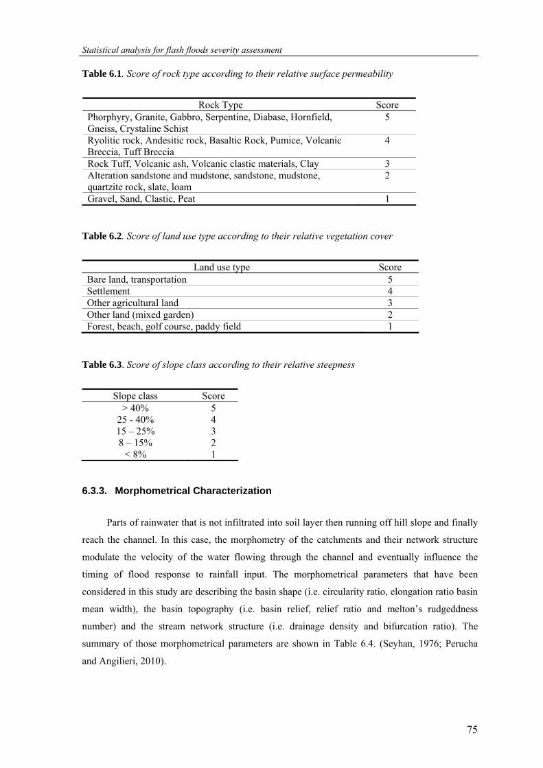
Statistical analysis for flash floods severity assessment
75
Table 6.1. Score of rock type according to their relative surface permeability
Rock Type Score
Phorphyry, Granite, Gabbro, Serpentine, Diabase, Hornfield, Gneiss, Crystaline Schist
5
Ryolitic rock, Andesitic rock, Basaltic Rock, Pumice, Volcanic Breccia, Tuff Breccia
4
Rock Tuff, Volcanic ash, Volcanic clastic materials, Clay 3 Alteration sandstone and mudstone, sandstone, mudstone, quartzite rock, slate, loam
2
Gravel, Sand, Clastic, Peat 1
Table 6.2. Score of land use type according to their relative vegetation cover
Land use type Score
Bare land, transportation 5 Settlement 4 Other agricultural land 3 Other land (mixed garden) 2 Forest, beach, golf course, paddy field 1
Table 6.3. Score of slope class according to their relative steepness
Slope class Score
> 40% 5 25 - 40% 4 15 – 25% 3 8 – 15% 2
< 8% 1
6.3.3. Morphometrical Characterization
Parts of rainwater that is not infiltrated into soil layer then running off hill slope and finally
reach the channel. In this case, the morphometry of the catchments and their network structure
modulate the velocity of the water flowing through the channel and eventually influence the
timing of flood response to rainfall input. The morphometrical parameters that have been
considered in this study are describing the basin shape (i.e. circularity ratio, elongation ratio basin
mean width), the basin topography (i.e. basin relief, relief ratio and melton’s rudgeddness
number) and the stream network structure (i.e. drainage density and bifurcation ratio). The
summary of those morphometrical parameters are shown in Table 6.4. (Seyhan, 1976; Perucha
and Angilieri, 2010).
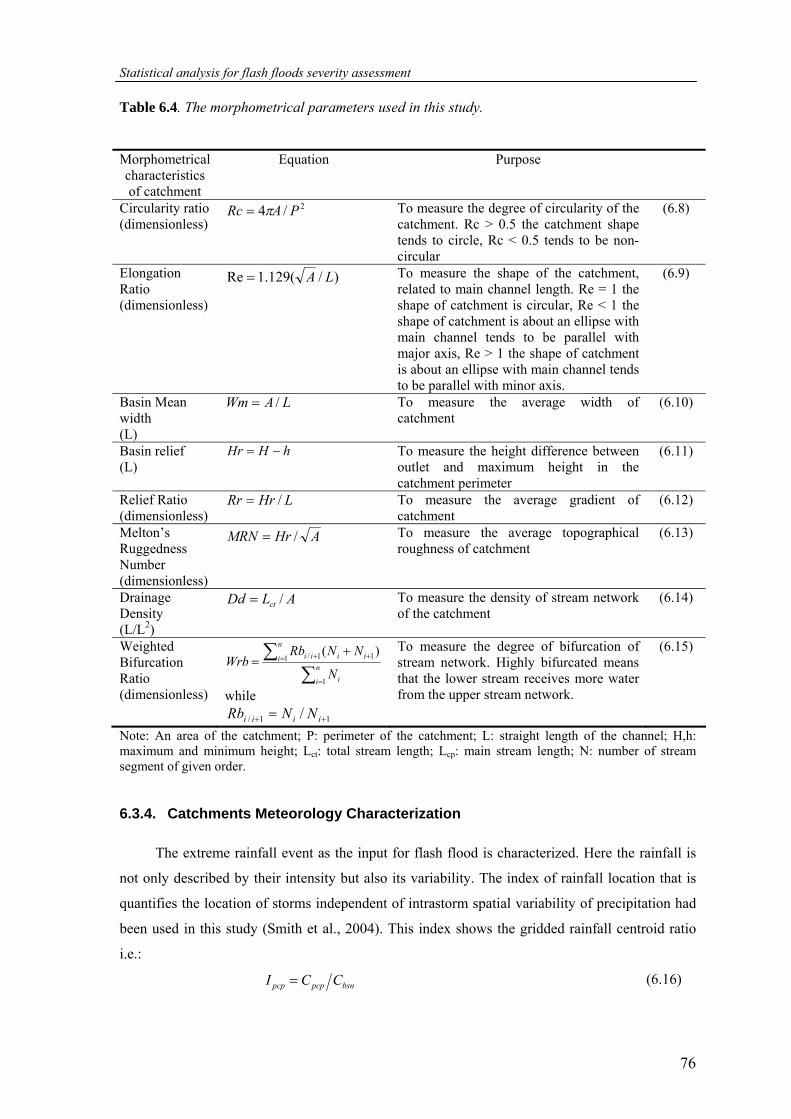
Statistical analysis for flash floods severity assessment
76
Table 6.4. The morphometrical parameters used in this study.
Morphometrical characteristics of catchment
Equation Purpose
Circularity ratio (dimensionless)
2/4 PARc π= To measure the degree of circularity of the catchment. Rc > 0.5 the catchment shape tends to circle, Rc < 0.5 tends to be non-circular
(6.8)
Elongation Ratio (dimensionless)
)/(129.1Re LA= To measure the shape of the catchment, related to main channel length. Re = 1 the shape of catchment is circular, Re < 1 the shape of catchment is about an ellipse with main channel tends to be parallel with major axis, Re > 1 the shape of catchment is about an ellipse with main channel tends to be parallel with minor axis.
(6.9)
Basin Mean width (L)
LAWm /= To measure the average width of catchment
(6.10)
Basin relief (L)
hHHr −= To measure the height difference between outlet and maximum height in the catchment perimeter
(6.11)
Relief Ratio (dimensionless)
LHrRr /= To measure the average gradient of catchment
(6.12)
Melton’s Ruggedness Number (dimensionless)
AHrMRN /= To measure the average topographical roughness of catchment
(6.13)
Drainage Density (L/L2)
ALDd ct /= To measure the density of stream network of the catchment
(6.14)
Weighted Bifurcation Ratio (dimensionless)
∑∑
=
= ++ += n
i i
n
i iiii
N
NNRbWrb
1
1 11/ )(
while 11/ / ++ = iiii NNRb
To measure the degree of bifurcation of stream network. Highly bifurcated means that the lower stream receives more water from the upper stream network.
(6.15)
Note: An area of the catchment; P: perimeter of the catchment; L: straight length of the channel; H,h: maximum and minimum height; Lct: total stream length; Lcp: main stream length; N: number of stream segment of given order.
6.3.4. Catchments Meteorology Characterization
The extreme rainfall event as the input for flash flood is characterized. Here the rainfall is
not only described by their intensity but also its variability. The index of rainfall location that is
quantifies the location of storms independent of intrastorm spatial variability of precipitation had
been used in this study (Smith et al., 2004). This index shows the gridded rainfall centroid ratio
i.e.:
bsnpcppcp CCI = (6.16)
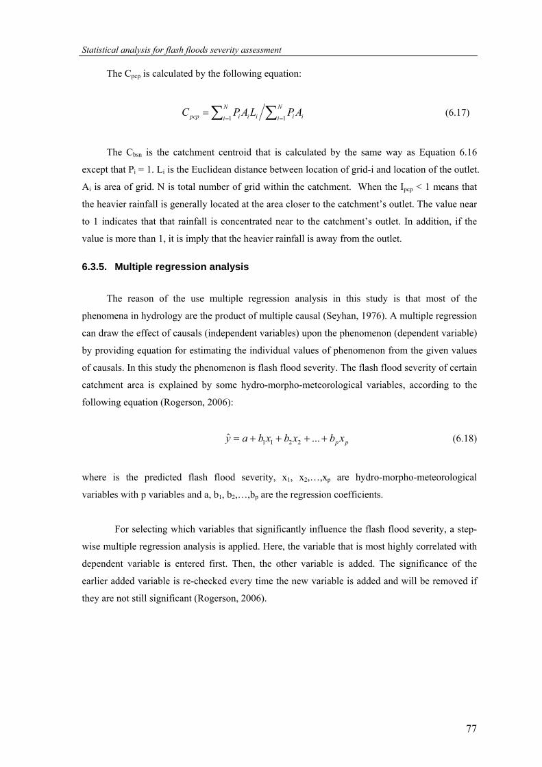
Statistical analysis for flash floods severity assessment
77
The Cpcp is calculated by the following equation:
∑∑ ===
N
i iiN
i iiipcp APLAPC11
(6.17)
The Cbsn is the catchment centroid that is calculated by the same way as Equation 6.16
except that Pi = 1. Li is the Euclidean distance between location of grid-i and location of the outlet.
Ai is area of grid. N is total number of grid within the catchment. When the Ipcp < 1 means that
the heavier rainfall is generally located at the area closer to the catchment’s outlet. The value near
to 1 indicates that that rainfall is concentrated near to the catchment’s outlet. In addition, if the
value is more than 1, it is imply that the heavier rainfall is away from the outlet.
6.3.5. Multiple regression analysis
The reason of the use multiple regression analysis in this study is that most of the
phenomena in hydrology are the product of multiple causal (Seyhan, 1976). A multiple regression
can draw the effect of causals (independent variables) upon the phenomenon (dependent variable)
by providing equation for estimating the individual values of phenomenon from the given values
of causals. In this study the phenomenon is flash flood severity. The flash flood severity of certain
catchment area is explained by some hydro-morpho-meteorological variables, according to the
following equation (Rogerson, 2006):
pp xbxbxbay ++++= ...ˆ 2211 (6.18)
where is the predicted flash flood severity, x1, x2,…,xp are hydro-morpho-meteorological
variables with p variables and a, b1, b2,…,bp are the regression coefficients.
For selecting which variables that significantly influence the flash flood severity, a step-
wise multiple regression analysis is applied. Here, the variable that is most highly correlated with
dependent variable is entered first. Then, the other variable is added. The significance of the
earlier added variable is re-checked every time the new variable is added and will be removed if
they are not still significant (Rogerson, 2006).
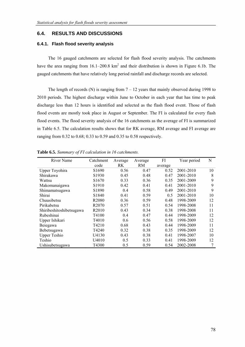
Statistical analysis for flash floods severity assessment
78
6.4. RESULTS AND DISCUSSIONS
6.4.1. Flash flood severity analysis
The 16 gauged catchments are selected for flash flood severity analysis. The catchments
have the area ranging from 16.1–200.8 km2 and their distribution is shown in Figure 6.1b. The
gauged catchments that have relatively long period rainfall and discharge records are selected.
The length of records (N) is ranging from 7 – 12 years that mainly observed during 1998 to
2010 periods. The highest discharge within June to October in each year that has time to peak
discharge less than 12 hours is identified and selected as the flash flood event. Those of flash
flood events are mostly took place in August or September. The FI is calculated for every flash
flood events. The flood severity analysis of the 16 catchments as the average of FI is summarized
in Table 6.5. The calculation results shows that for RK average, RM average and FI average are
ranging from 0.32 to 0.68; 0.33 to 0.59 and 0.35 to 0.58 respectively.
Table 6.5. Summary of FI calculation in 16 catchments.
River Name Catchment code
Average RK
Average RM
FI average
Year period N
Upper Toyohira S1690 0.56 0.47 0.52 2001-2010 10 Shirakawa S1930 0.45 0.48 0.47 2001-2010 8 Wattsu S1670 0.33 0.36 0.35 2001-2009 9 Makomanaigawa S1910 0.42 0.41 0.41 2001-2010 9 Shimamatsugawa S1890 0.4 0.58 0.49 2001-2010 9 Shirai S1840 0.41 0.59 0.5 2001-2010 10 Chuusibetsu R2080 0.36 0.59 0.48 1998-2009 12 Pirikabetsu R2070 0.57 0.51 0.54 1998-2008 11 Shiribeshitoshibetsugawa R2010 0.43 0.34 0.38 1998-2008 11 Rubeshinai T4100 0.4 0.47 0.44 1998-2009 12 Upper Ishikari T4010 0.6 0.56 0.58 1998-2009 12 Beiegawa T4210 0.68 0.43 0.44 1998-2009 11 Bebetsugawa T4240 0.32 0.38 0.35 1998-2009 12 Upper Teshio U4130 0.43 0.38 0.41 1998-2007 10 Teshio U4010 0.5 0.33 0.41 1998-2009 12 Ushisubetsugawa T4300 0.5 0.59 0.54 2002-2008 7
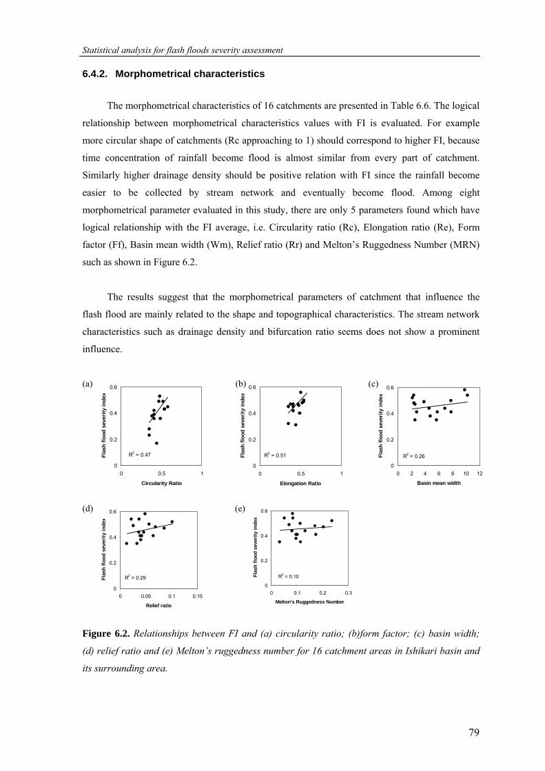
Statistical analysis for flash floods severity assessment
79
R2 = 0.47
0
0.2
0.4
0.6
0 0.5 1
Circularity Ratio
Flas
h flo
od s
ever
ity in
dex
R2 = 0.51
0
0.2
0.4
0.6
0 0.5 1
Elongation Ratio
Flas
h flo
od s
ever
ity in
dex
R2 = 0.26
0
0.2
0.4
0.6
0 2 4 6 8 10 12
Basin mean width
Flas
h flo
od s
ever
ity in
dex
R2 = 0.29
0
0.2
0.4
0.6
0 0.05 0.1 0.15
Relief ratio
Flas
h flo
od s
ever
ity in
dex
R2 = 0.10
0
0.2
0.4
0.6
0 0.1 0.2 0.3
Melton's Ruggedness Number
Flas
h flo
od s
ever
ity in
dex
6.4.2. Morphometrical characteristics
The morphometrical characteristics of 16 catchments are presented in Table 6.6. The logical
relationship between morphometrical characteristics values with FI is evaluated. For example
more circular shape of catchments (Rc approaching to 1) should correspond to higher FI, because
time concentration of rainfall become flood is almost similar from every part of catchment.
Similarly higher drainage density should be positive relation with FI since the rainfall become
easier to be collected by stream network and eventually become flood. Among eight
morphometrical parameter evaluated in this study, there are only 5 parameters found which have
logical relationship with the FI average, i.e. Circularity ratio (Rc), Elongation ratio (Re), Form
factor (Ff), Basin mean width (Wm), Relief ratio (Rr) and Melton’s Ruggedness Number (MRN)
such as shown in Figure 6.2.
The results suggest that the morphometrical parameters of catchment that influence the
flash flood are mainly related to the shape and topographical characteristics. The stream network
characteristics such as drainage density and bifurcation ratio seems does not show a prominent
influence.
(a) (b) (c)
(d) (e)
Figure 6.2. Relationships between FI and (a) circularity ratio; (b)form factor; (c) basin width;
(d) relief ratio and (e) Melton’s ruggedness number for 16 catchment areas in Ishikari basin and
its surrounding area.
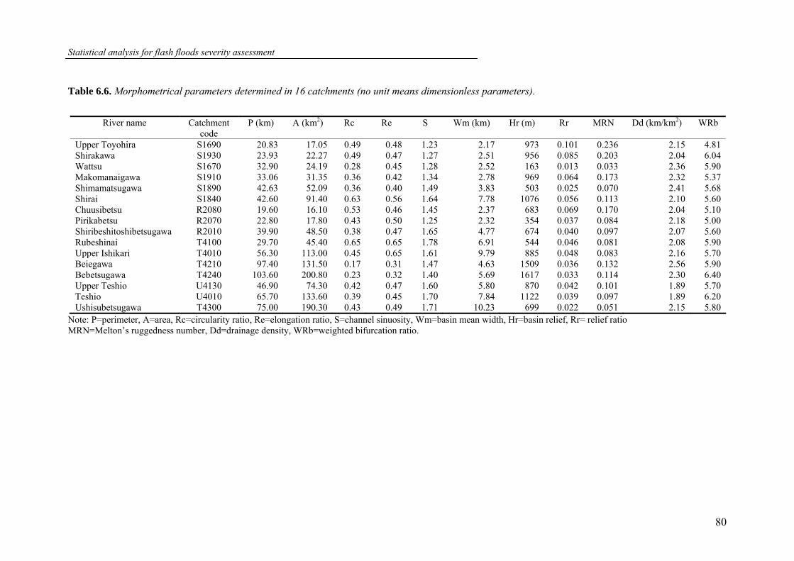
Statistical analysis for flash floods severity assessment
80
Table 6.6. Morphometrical parameters determined in 16 catchments (no unit means dimensionless parameters).
River name Catchment
code P (km) A (km2) Rc Re S Wm (km) Hr (m) Rr MRN Dd (km/km2) WRb
Upper Toyohira S1690 20.83 17.05 0.49 0.48 1.23 2.17 973 0.101 0.236 2.15 4.81 Shirakawa S1930 23.93 22.27 0.49 0.47 1.27 2.51 956 0.085 0.203 2.04 6.04 Wattsu S1670 32.90 24.19 0.28 0.45 1.28 2.52 163 0.013 0.033 2.36 5.90 Makomanaigawa S1910 33.06 31.35 0.36 0.42 1.34 2.78 969 0.064 0.173 2.32 5.37 Shimamatsugawa S1890 42.63 52.09 0.36 0.40 1.49 3.83 503 0.025 0.070 2.41 5.68 Shirai S1840 42.60 91.40 0.63 0.56 1.64 7.78 1076 0.056 0.113 2.10 5.60 Chuusibetsu R2080 19.60 16.10 0.53 0.46 1.45 2.37 683 0.069 0.170 2.04 5.10 Pirikabetsu R2070 22.80 17.80 0.43 0.50 1.25 2.32 354 0.037 0.084 2.18 5.00 Shiribeshitoshibetsugawa R2010 39.90 48.50 0.38 0.47 1.65 4.77 674 0.040 0.097 2.07 5.60 Rubeshinai T4100 29.70 45.40 0.65 0.65 1.78 6.91 544 0.046 0.081 2.08 5.90 Upper Ishikari T4010 56.30 113.00 0.45 0.65 1.61 9.79 885 0.048 0.083 2.16 5.70 Beiegawa T4210 97.40 131.50 0.17 0.31 1.47 4.63 1509 0.036 0.132 2.56 5.90 Bebetsugawa T4240 103.60 200.80 0.23 0.32 1.40 5.69 1617 0.033 0.114 2.30 6.40 Upper Teshio U4130 46.90 74.30 0.42 0.47 1.60 5.80 870 0.042 0.101 1.89 5.70 Teshio U4010 65.70 133.60 0.39 0.45 1.70 7.84 1122 0.039 0.097 1.89 6.20 Ushisubetsugawa T4300 75.00 190.30 0.43 0.49 1.71 10.23 699 0.022 0.051 2.15 5.80
Note: P=perimeter, A=area, Rc=circularity ratio, Re=elongation ratio, S=channel sinuosity, Wm=basin mean width, Hr=basin relief, Rr= relief ratio MRN=Melton’s ruggedness number, Dd=drainage density, WRb=weighted bifurcation ratio.
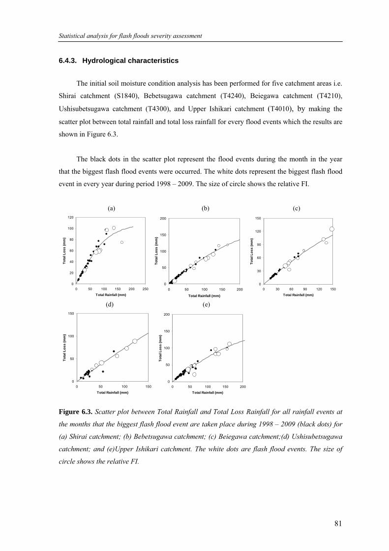
Statistical analysis for flash floods severity assessment
81
6.4.3. Hydrological characteristics
The initial soil moisture condition analysis has been performed for five catchment areas i.e.
Shirai catchment (S1840), Bebetsugawa catchment (T4240), Beiegawa catchment (T4210),
Ushisubetsugawa catchment (T4300), and Upper Ishikari catchment (T4010), by making the
scatter plot between total rainfall and total loss rainfall for every flood events which the results are
shown in Figure 6.3.
The black dots in the scatter plot represent the flood events during the month in the year
that the biggest flash flood events were occurred. The white dots represent the biggest flash flood
event in every year during period 1998 – 2009. The size of circle shows the relative FI.
(a) (b) (c)
0
20
40
60
80
100
120
0 50 100 150 200 250
Total Rainfall (mm)
Tota
l Los
s (m
m)
0
50
100
150
200
0 50 100 150 200
Total Rainfall (mm)
Tota
l Los
s (m
m)
0
30
60
90
120
150
0 30 60 90 120 150
Total Rainfall (mm)
Tota
l Los
s (m
m)
(d) (e)
0
50
100
150
0 50 100 150
Total Rainfall (mm)
Tota
l Los
s (m
m)
0
50
100
150
200
0 50 100 150 200
Total Rainfall (mm)
Tota
l Los
s (m
m)
Figure 6.3. Scatter plot between Total Rainfall and Total Loss Rainfall for all rainfall events at
the months that the biggest flash flood event are taken place during 1998 – 2009 (black dots) for
(a) Shirai catchment; (b) Bebetsugawa catchment; (c) Beiegawa catchment;(d) Ushisubetsugawa
catchment; and (e)Upper Ishikari catchment. The white dots are flash flood events. The size of
circle shows the relative FI.
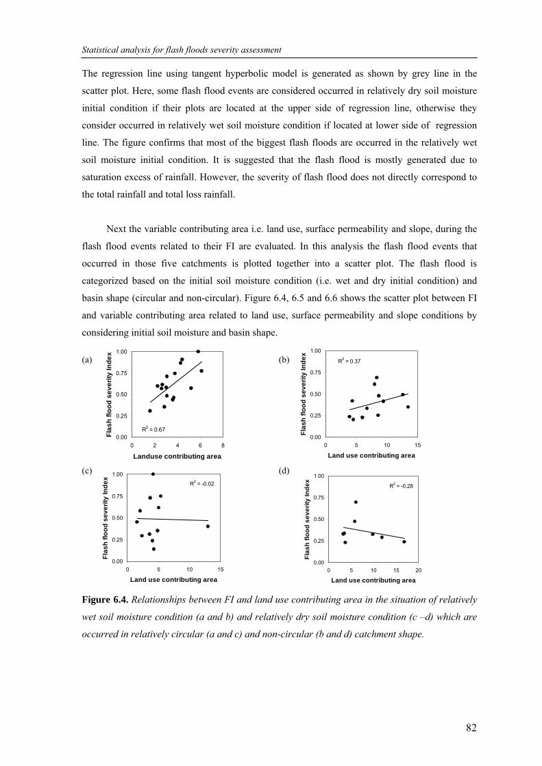
Statistical analysis for flash floods severity assessment
82
R2 = 0.670.00
0.25
0.50
0.75
1.00
0 2 4 6 8
Landuse contributing area
Flas
h flo
od s
ever
ity In
dex
R2 = 0.37
0.00
0.25
0.50
0.75
1.00
0 5 10 15
Land use contributing area
Flas
h flo
od s
ever
ity In
dex
R2 = -0.02
0.00
0.25
0.50
0.75
1.00
0 5 10 15
Land use contributing area
Flas
h flo
od s
ever
ity In
dex
R2 = -0.28
0.00
0.25
0.50
0.75
1.00
0 5 10 15 20
Land use contributing area
Flas
h flo
od s
ever
ity In
dex
The regression line using tangent hyperbolic model is generated as shown by grey line in the
scatter plot. Here, some flash flood events are considered occurred in relatively dry soil moisture
initial condition if their plots are located at the upper side of regression line, otherwise they
consider occurred in relatively wet soil moisture condition if located at lower side of regression
line. The figure confirms that most of the biggest flash floods are occurred in the relatively wet
soil moisture initial condition. It is suggested that the flash flood is mostly generated due to
saturation excess of rainfall. However, the severity of flash flood does not directly correspond to
the total rainfall and total loss rainfall.
Next the variable contributing area i.e. land use, surface permeability and slope, during the
flash flood events related to their FI are evaluated. In this analysis the flash flood events that
occurred in those five catchments is plotted together into a scatter plot. The flash flood is
categorized based on the initial soil moisture condition (i.e. wet and dry initial condition) and
basin shape (circular and non-circular). Figure 6.4, 6.5 and 6.6 shows the scatter plot between FI
and variable contributing area related to land use, surface permeability and slope conditions by
considering initial soil moisture and basin shape. (a) (b)
(c) (d)
Figure 6.4. Relationships between FI and land use contributing area in the situation of relatively
wet soil moisture condition (a and b) and relatively dry soil moisture condition (c –d) which are
occurred in relatively circular (a and c) and non-circular (b and d) catchment shape.
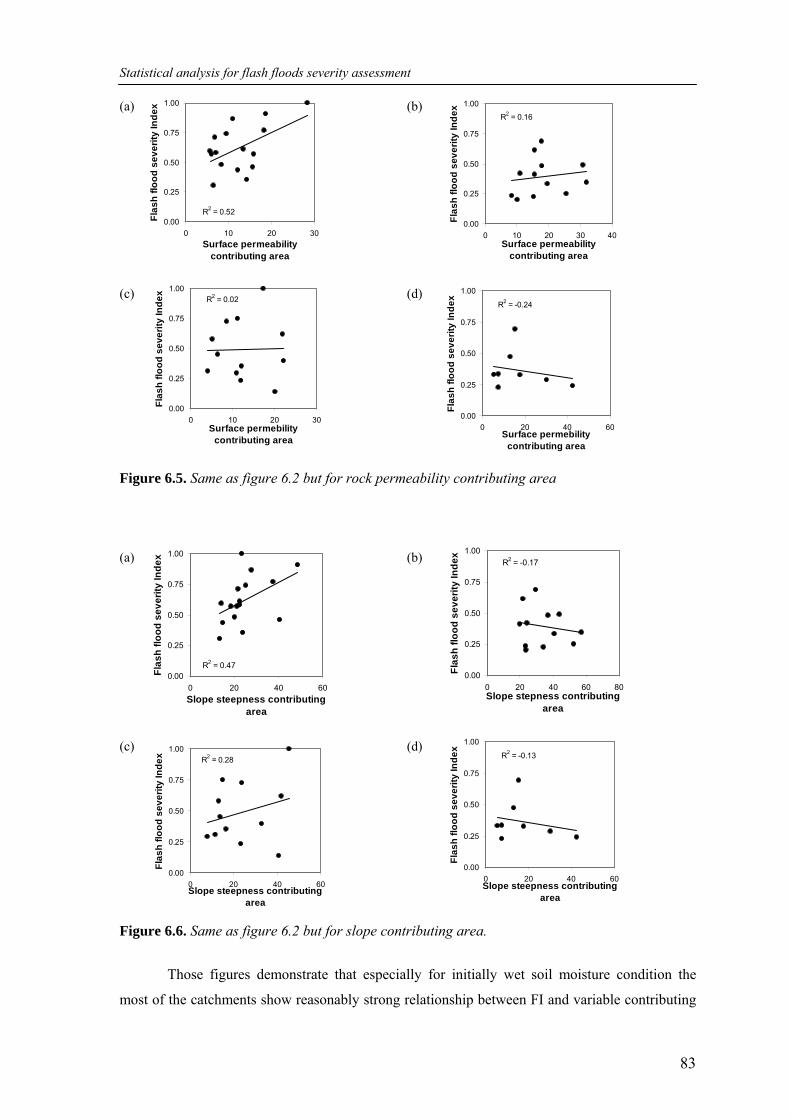
Statistical analysis for flash floods severity assessment
83
R2 = 0.520.00
0.25
0.50
0.75
1.00
0 10 20 30Surface permeability
contributing area
Flas
h flo
od s
ever
ity In
dex
R2 = 0.16
0.00
0.25
0.50
0.75
1.00
0 10 20 30 40Surface permeability
contributing area
Flas
h flo
od s
ever
ity In
dex
R2 = 0.02
0.00
0.25
0.50
0.75
1.00
0 10 20 30Surface permebility
contributing area
Flas
h flo
od s
ever
ity In
dex
R2 = -0.24
0.00
0.25
0.50
0.75
1.00
0 20 40 60Surface permebility
contributing areaFl
ash
flood
sev
erity
Inde
x
R2 = 0.470.00
0.25
0.50
0.75
1.00
0 20 40 60Slope steepness contributing
area
Flas
h flo
od s
ever
ity In
dex R2 = -0.17
0.00
0.25
0.50
0.75
1.00
0 20 40 60 80Slope stepness contributing
area
Flas
h flo
od s
ever
ity In
dex
R2 = 0.28
0.00
0.25
0.50
0.75
1.00
0 20 40 60Slope steepness contributing
area
Flas
h flo
od s
ever
ity In
dex R2 = -0.13
0.00
0.25
0.50
0.75
1.00
0 20 40 60Slope steepness contributing
area
Flas
h flo
od s
ever
ity In
dex
(a) (b)
(c) (d) Figure 6.5. Same as figure 6.2 but for rock permeability contributing area
(a) (b)
(c) (d) Figure 6.6. Same as figure 6.2 but for slope contributing area.
Those figures demonstrate that especially for initially wet soil moisture condition the
most of the catchments show reasonably strong relationship between FI and variable contributing
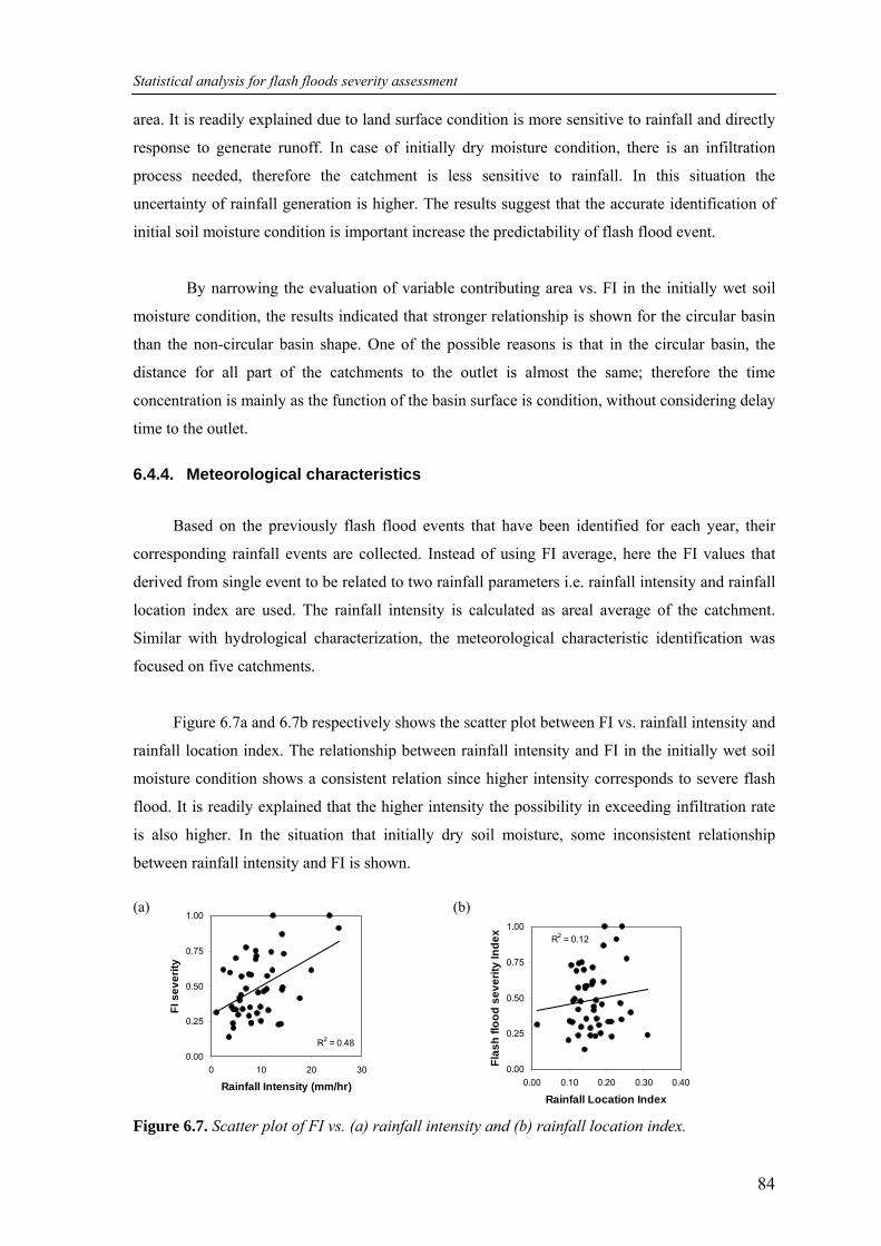
Statistical analysis for flash floods severity assessment
84
R2 = 0.480.00
0.25
0.50
0.75
1.00
0 10 20 30
Rainfall Intensity (mm/hr)
FI s
ever
ity
R2 = 0.12
0.00
0.25
0.50
0.75
1.00
0.00 0.10 0.20 0.30 0.40
Rainfall Location Index
Flas
h flo
od s
ever
ity In
dex
area. It is readily explained due to land surface condition is more sensitive to rainfall and directly
response to generate runoff. In case of initially dry moisture condition, there is an infiltration
process needed, therefore the catchment is less sensitive to rainfall. In this situation the
uncertainty of rainfall generation is higher. The results suggest that the accurate identification of
initial soil moisture condition is important increase the predictability of flash flood event.
By narrowing the evaluation of variable contributing area vs. FI in the initially wet soil
moisture condition, the results indicated that stronger relationship is shown for the circular basin
than the non-circular basin shape. One of the possible reasons is that in the circular basin, the
distance for all part of the catchments to the outlet is almost the same; therefore the time
concentration is mainly as the function of the basin surface is condition, without considering delay
time to the outlet.
6.4.4. Meteorological characteristics
Based on the previously flash flood events that have been identified for each year, their
corresponding rainfall events are collected. Instead of using FI average, here the FI values that
derived from single event to be related to two rainfall parameters i.e. rainfall intensity and rainfall
location index are used. The rainfall intensity is calculated as areal average of the catchment.
Similar with hydrological characterization, the meteorological characteristic identification was
focused on five catchments.
Figure 6.7a and 6.7b respectively shows the scatter plot between FI vs. rainfall intensity and
rainfall location index. The relationship between rainfall intensity and FI in the initially wet soil
moisture condition shows a consistent relation since higher intensity corresponds to severe flash
flood. It is readily explained that the higher intensity the possibility in exceeding infiltration rate
is also higher. In the situation that initially dry soil moisture, some inconsistent relationship
between rainfall intensity and FI is shown. (a) (b) Figure 6.7. Scatter plot of FI vs. (a) rainfall intensity and (b) rainfall location index.
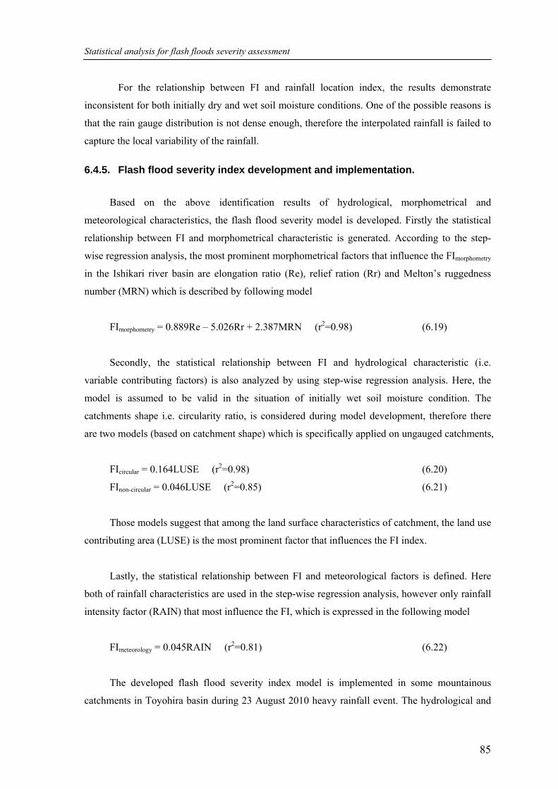
Statistical analysis for flash floods severity assessment
85
For the relationship between FI and rainfall location index, the results demonstrate
inconsistent for both initially dry and wet soil moisture conditions. One of the possible reasons is
that the rain gauge distribution is not dense enough, therefore the interpolated rainfall is failed to
capture the local variability of the rainfall.
6.4.5. Flash flood severity index development and implementation.
Based on the above identification results of hydrological, morphometrical and
meteorological characteristics, the flash flood severity model is developed. Firstly the statistical
relationship between FI and morphometrical characteristic is generated. According to the step-
wise regression analysis, the most prominent morphometrical factors that influence the FImorphometry
in the Ishikari river basin are elongation ratio (Re), relief ration (Rr) and Melton’s ruggedness
number (MRN) which is described by following model
FImorphometry = 0.889Re – 5.026Rr + 2.387MRN (r2=0.98) (6.19)
Secondly, the statistical relationship between FI and hydrological characteristic (i.e.
variable contributing factors) is also analyzed by using step-wise regression analysis. Here, the
model is assumed to be valid in the situation of initially wet soil moisture condition. The
catchments shape i.e. circularity ratio, is considered during model development, therefore there
are two models (based on catchment shape) which is specifically applied on ungauged catchments,
FIcircular = 0.164LUSE (r2=0.98) (6.20)
FInon-circular = 0.046LUSE (r2=0.85) (6.21)
Those models suggest that among the land surface characteristics of catchment, the land use
contributing area (LUSE) is the most prominent factor that influences the FI index.
Lastly, the statistical relationship between FI and meteorological factors is defined. Here
both of rainfall characteristics are used in the step-wise regression analysis, however only rainfall
intensity factor (RAIN) that most influence the FI, which is expressed in the following model
FImeteorology = 0.045RAIN (r2=0.81) (6.22)
The developed flash flood severity index model is implemented in some mountainous
catchments in Toyohira basin during 23 August 2010 heavy rainfall event. The hydrological and
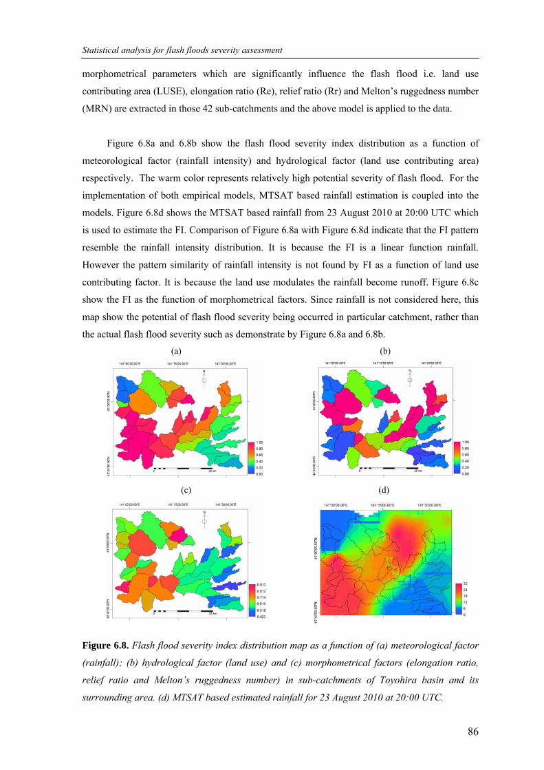
Statistical analysis for flash floods severity assessment
86
morphometrical parameters which are significantly influence the flash flood i.e. land use
contributing area (LUSE), elongation ratio (Re), relief ratio (Rr) and Melton’s ruggedness number
(MRN) are extracted in those 42 sub-catchments and the above model is applied to the data.
Figure 6.8a and 6.8b show the flash flood severity index distribution as a function of
meteorological factor (rainfall intensity) and hydrological factor (land use contributing area)
respectively. The warm color represents relatively high potential severity of flash flood. For the
implementation of both empirical models, MTSAT based rainfall estimation is coupled into the
models. Figure 6.8d shows the MTSAT based rainfall from 23 August 2010 at 20:00 UTC which
is used to estimate the FI. Comparison of Figure 6.8a with Figure 6.8d indicate that the FI pattern
resemble the rainfall intensity distribution. It is because the FI is a linear function rainfall.
However the pattern similarity of rainfall intensity is not found by FI as a function of land use
contributing factor. It is because the land use modulates the rainfall become runoff. Figure 6.8c
show the FI as the function of morphometrical factors. Since rainfall is not considered here, this
map show the potential of flash flood severity being occurred in particular catchment, rather than
the actual flash flood severity such as demonstrate by Figure 6.8a and 6.8b. (a) (b)
(c) (d)
Figure 6.8. Flash flood severity index distribution map as a function of (a) meteorological factor
(rainfall); (b) hydrological factor (land use) and (c) morphometrical factors (elongation ratio,
relief ratio and Melton’s ruggedness number) in sub-catchments of Toyohira basin and its
surrounding area. (d) MTSAT based estimated rainfall for 23 August 2010 at 20:00 UTC.
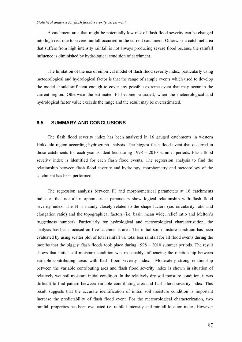
Statistical analysis for flash floods severity assessment
87
A catchment area that might be potentially low risk of flash flood severity can be changed
into high risk due to severe rainfall occurred in the current catchment. Otherwise a catchmet area
that suffers from high intensity rainfall is not always producing severe flood because the rainfall
influence is diminished by hydrological condition of catchment.
The limitation of the use of empirical model of flash flood severity index, particularly using
meteorological and hydrological factor is that the range of sample events which used to develop
the model should sufficient enough to cover any possible extreme event that may occur in the
current region. Otherwise the estimated FI become saturated, when the meteorological and
hydrological factor value exceeds the range and the result may be overestimated.
6.5. SUMMARY AND CONCLUSIONS
The flash flood severity index has been analyzed in 16 gauged catchments in western
Hokkaido region according hydrograph analysis. The biggest flash flood event that occurred in
those catchments for each year is identified during 1998 – 2010 summer periods. Flash flood
severity index is identified for each flash flood events. The regression analysis to find the
relationship between flash flood severity and hydrology, morphometry and meteorology of the
catchment has been performed.
The regression analysis between FI and morphometrical parameters at 16 catchments
indicates that not all morphometrical parameters show logical relationship with flash flood
severity index. The FI is mainly closely related to the shape factors (i.e. circularity ratio and
elongation ratio) and the topographical factors (i.e. basin mean wide, relief ratio and Melton’s
ruggedness number). Particularly for hydrological and meteorological characterization, the
analysis has been focused on five catchments area. The initial soil moisture condition has been
evaluated by using scatter plot of total rainfall vs. total loss rainfall for all flood events during the
months that the biggest flash floods took place during 1998 – 2010 summer periods. The result
shows that initial soil moisture condition was reasonably influencing the relationship between
variable contributing areas with flash flood severity index. Moderately strong relationship
between the variable contributing area and flash flood severity index is shown in situation of
relatively wet soil moisture initial condition. In the relatively dry soil moisture condition, it was
difficult to find pattern between variable contributing area and flash flood severity index. This
result suggests that the accurate identification of initial soil moisture condition is important
increase the predictability of flash flood event. For the meteorological characterization, two
rainfall properties has been evaluated i.e. rainfall intensity and rainfall location index. However

Statistical analysis for flash floods severity assessment
88
the results show that only rainfall intensity demonstrates strong relationship with flash flood
severity index. The implementation of the empirical models at Toyohira basin shows that FI as the
function of morphometrical factors can provide flash flood potential information. Moreover, FI as
the function of hydrological and meteorological factors demonstrate more dynamic pattern since
they correspond to rainfall distribution.
Chapter 7. PHYSICAL BASED RAINFALL-RUNOFF MODEL FOR FLASH FLOODS ESTIMATION
This chapter is based on: Suseno, Dwi Prabowo Yuga, T. J. Yamada, 2013, The use of Geostationary
Satellite Based Rainfall Estimation Combined With Land Surface Model for Regional Flash Flood
Assessment, to be presented on The 6th conference of The Asia Pacific Association of Hydrology and
Water Resources, Seoul, Korea
Physical Process Based Rainfall-Runoff Model For Flash Floods Estimation
90
Abstract
An understanding of hydrological behavior especially related to extreme event such as flash flood
is vital for flood mitigation and management. This study aims to assess the flash floods in a
regional scale by implementing the Minimal Advance Treatments of Surface Interaction and
Runoff (MATSIRO). MATSIRO is originally designed for global scale hydrological study and
using various data forcing both atmospheric and land surface forcing. In this study, they are
downscaled into regional scale. In order to make the model more applicable particularly to the
region that the availability of meteorological data is lacking, the use of remote sensing to acquire
some data input has been focused. Several remote sensing sensors such as Moderate Resolution
Imaging Spectroradiometer (MODIS) and Clouds and the Earth's Radiant Energy System
(CERES) sensors had been utilized to derive several distributed parameter such as leaf area index
(LAI), ground albedo, downward radiation (shortwave and longwave) and land cover. Moreover,
digital elevation model (DEM) obtained by Shuttle Radar Topographic Mission (SRTM) was
implemented to quantify some topographic and river flow parameters. Specifically for the rainfall
forcing, it is generated from the Multifunctional Transport Satellite (MTSAT) based rainfall
estimation which is downscaled by using local observed rainfall (Automated Meteorological Data
Acquisition System/AMeDAS). The river flow simulations were run over Ishikari river basin in 1-
km grid resolution by using three rainfall data forcing i.e. AMeDAS rainfall, MTSAT based
estimated rainfall and Ministry of Land, Infrastructure and Transport (MLIT) rainfall. A
comparison of estimated peak discharge resulted by those simulations with observed stream flow
is performed and evaluated. The river flow simulations demonstrate that the MLIT rainfall based
estimated discharge is the best in predicting peak discharge. However, MTSAT downscaled
demonstrate more advantage as input forcing in the MATSIRO because the performance is about
comparable with the relatively dense rain gauge network such as the MLIT.
Key Words: MATSIRO, rainfall estimation, flash flood assessment, river flow simulation
Physical Process Based Rainfall-Runoff Model For Flash Floods Estimation
91
7.1. INTRODUCTION
An understanding of hydrological behavior of a catchment area especially related to
extreme event such as flash flood is vital for flood mitigation and management. Some studies
related to flash flood study for mitigation has been conducted such as risk estimation (Yousef et
al., 2010), early detection (Alfieri et al, 2012) and severity (Bashkar et al, 2000; Kim and Choi,
2011; 2012). Due to the importance of flash flood information such as their risk and early warning,
such information should be provided all over the region, particularly those vulnerable to flash
flood. The magnitude of peak discharge and its time to peak discharge during flash flood event are
considered as the important parameters that should be provided for mitigating their disastrous
effect. Those information usually are derived by analyzing the discharge that measured by water
level recorder instrument installed at the catchment’s outlet. However, this effort mainly
hampered due to the shortage of data. It is because not all catchments are equipped with discharge
measurement instrument. Missing of data is often to be happened due to the river gauges have
damaged by severe flash flood. As an alternative way for obtaining such hydrological data,
instead of using direct measurement, the rainfall-runoff model is utilized to get simulated
discharge.
The rainfall observation network data is commonly employed as the input data for the
rainfall-runoff model. However it has disadvantage due to sparse and uneven distribution in space.
The limitation of fund, accessibility of the site and the purpose of network is considered as
constraint for developing high density and well configuration of rain gauge network (Haile, 2011).
Radar can be used to obtain the spatial distribution of rainfall, however this method is considered
too expensive. The high mountainous range that can block the radar signal is also considered as
another restriction. The geostationary based rainfall estimation gives an opportunity for providing
continuous rainfall information particularly for the ungauged catchments (Kinoti et al, 2010,
Suseno and Yamada, 2013a). The geostationary satellite image which is blended with microwave
satellite based rainfall measurement is preferable instead of the use of microwave satellite based
rainfall measurement solely. It is because the geostationary satellite has advantage for capturing
global coverage with continuous acquisition time which is very useful for monitoring purpose.
The geostationary based rainfall estimation can be coupled with a rainfall-runoff model for
predicting the flood discharge produce by a catchment (Wardah et al., 2008).
Hapuarachchi et al. (2011) conducted a review of advances in flash flood forecasting and
notify that the physically based hydrological model particularly the distributed model give more
plausible results when compared with the results of conceptual, statistical and neural network
model. This study intends to conduct a flash flood assessment based on a physically based
Physical Process Based Rainfall-Runoff Model For Flash Floods Estimation
92
hydrological model called the Minimal Advance Treatments of Surface Interaction and Runoff
(MATSIRO). The term ‘advance’ in this model is related to the physically based that used by
model and term ‘minimal’ means that the water and energy exchange between land and
atmosphere represented by model had been treated by simple manner (Takata et al., 2003).
MATSIRO uses physical process to draw the hydro-meteorological characteristics of a region
which is expressed by the energy balance model and the water balance model. The energy balance
model is calculated based on those two models, the surface energy flux and land surface
interaction among main hydrological components (i.e. precipitation, evapotranspiration, moisture
storage and surface flow) can be comprehensively evaluated. The recent implementation of
MATSIRO deals with its application for global (1°×1° grid size) and nation wide hydrological
study such as in Japan country with 10 km grid size (Pokhrel, 2011). In this study, the MATSIRO
was applied for flash floods assessment, for a regional scale, in approximately 1 km by 1 km grid
size.
More attentions have been paid in this study for acquiring some input data into MATSIRO
by using remote sensing techniques in order it can be applied to overcome the data shortage
problem. Rainfall estimation by using Multi-purpose Transport Satellite (MTSAT) (Suseno and
Yamada, 2013) is applied as forcing data into MATSIRO model. Some input parameters that
generated by remote sensing data is also utilized, such the use of digital elevation model from
Shuttle Radar Topographic Mission Digital Elevation Model (SRTM-DEM) and Moderate
Resolution Imaging Spectroradiometer (MODIS) sensors to derived surface topography data,
stream network and land cover.
The objectives of this study are (i) to generate some data forcing by using remote sensing
and to apply into MATSIRO and (ii) to perform a river flow simulation using MATSIRO and
compare estimated discharge obtained from the model with the observed discharge. The estimated
discharge is derived by using both observed rainfall and satellite based rainfall estimation.
7.2. THE STUDY AREA AND DATASETS
The study area is Ishikari river basin, Hokkaido Island, Japan (see grey area in Figure 7.1).
The time period during 2010 was examined for MATSIRO data forcing preparation process. The
MODIS sensors had been used to derive several distributed parameters such as leaf area index
(LAI), ground albedo and land cover. MODIS has high spectral resolution (36 spectral bands)
with various spatial resolutions (250m, 500m and 1km) depend on the channel.
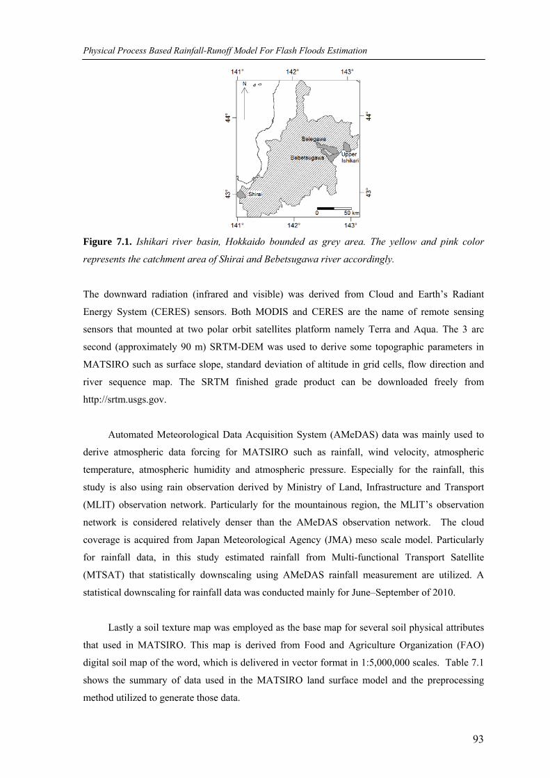
Physical Process Based Rainfall-Runoff Model For Flash Floods Estimation
93
Figure 7.1. Ishikari river basin, Hokkaido bounded as grey area. The yellow and pink color
represents the catchment area of Shirai and Bebetsugawa river accordingly.
The downward radiation (infrared and visible) was derived from Cloud and Earth’s Radiant
Energy System (CERES) sensors. Both MODIS and CERES are the name of remote sensing
sensors that mounted at two polar orbit satellites platform namely Terra and Aqua. The 3 arc
second (approximately 90 m) SRTM-DEM was used to derive some topographic parameters in
MATSIRO such as surface slope, standard deviation of altitude in grid cells, flow direction and
river sequence map. The SRTM finished grade product can be downloaded freely from
http://srtm.usgs.gov.
Automated Meteorological Data Acquisition System (AMeDAS) data was mainly used to
derive atmospheric data forcing for MATSIRO such as rainfall, wind velocity, atmospheric
temperature, atmospheric humidity and atmospheric pressure. Especially for the rainfall, this
study is also using rain observation derived by Ministry of Land, Infrastructure and Transport
(MLIT) observation network. Particularly for the mountainous region, the MLIT’s observation
network is considered relatively denser than the AMeDAS observation network. The cloud
coverage is acquired from Japan Meteorological Agency (JMA) meso scale model. Particularly
for rainfall data, in this study estimated rainfall from Multi-functional Transport Satellite
(MTSAT) that statistically downscaling using AMeDAS rainfall measurement are utilized. A
statistical downscaling for rainfall data was conducted mainly for June–September of 2010.
Lastly a soil texture map was employed as the base map for several soil physical attributes
that used in MATSIRO. This map is derived from Food and Agriculture Organization (FAO)
digital soil map of the word, which is delivered in vector format in 1:5,000,000 scales. Table 7.1
shows the summary of data used in the MATSIRO land surface model and the preprocessing
method utilized to generate those data.
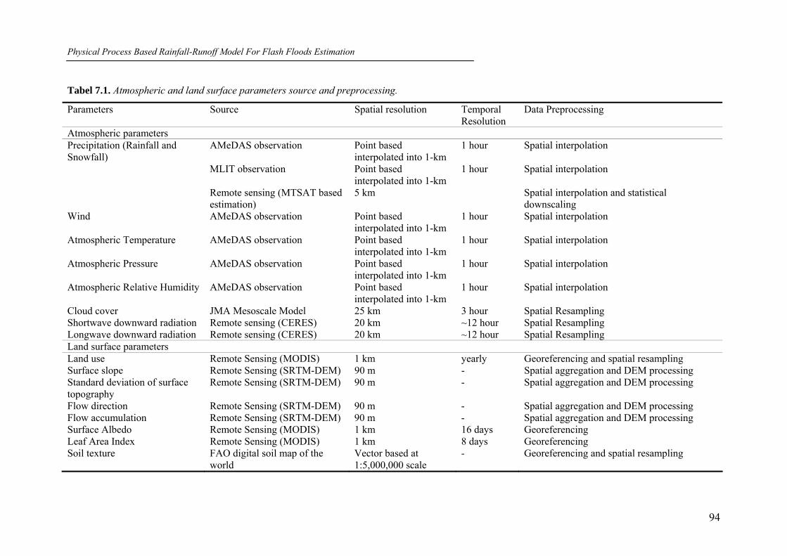
Physical Process Based Rainfall-Runoff Model For Flash Floods Estimation
94
Tabel 7.1. Atmospheric and land surface parameters source and preprocessing.
Parameters Source Spatial resolution Temporal Resolution
Data Preprocessing
Atmospheric parameters Precipitation (Rainfall and Snowfall)
AMeDAS observation MLIT observation Remote sensing (MTSAT based estimation)
Point based interpolated into 1-km Point based interpolated into 1-km 5 km
1 hour 1 hour
Spatial interpolation Spatial interpolation Spatial interpolation and statistical downscaling
Wind AMeDAS observation Point based interpolated into 1-km
1 hour Spatial interpolation
Atmospheric Temperature AMeDAS observation Point based interpolated into 1-km
1 hour Spatial interpolation
Atmospheric Pressure AMeDAS observation Point based interpolated into 1-km
1 hour Spatial interpolation
Atmospheric Relative Humidity AMeDAS observation Point based interpolated into 1-km
1 hour Spatial interpolation
Cloud cover JMA Mesoscale Model 25 km 3 hour Spatial Resampling Shortwave downward radiation Remote sensing (CERES) 20 km ~12 hour Spatial Resampling Longwave downward radiation Remote sensing (CERES) 20 km ~12 hour Spatial Resampling Land surface parameters Land use Remote Sensing (MODIS) 1 km yearly Georeferencing and spatial resampling Surface slope Remote Sensing (SRTM-DEM) 90 m - Spatial aggregation and DEM processing Standard deviation of surface topography
Remote Sensing (SRTM-DEM) 90 m - Spatial aggregation and DEM processing
Flow direction Remote Sensing (SRTM-DEM) 90 m - Spatial aggregation and DEM processing Flow accumulation Remote Sensing (SRTM-DEM) 90 m - Spatial aggregation and DEM processing Surface Albedo Remote Sensing (MODIS) 1 km 16 days Georeferencing Leaf Area Index Remote Sensing (MODIS) 1 km 8 days Georeferencing Soil texture FAO digital soil map of the
world Vector based at 1:5,000,000 scale
- Georeferencing and spatial resampling
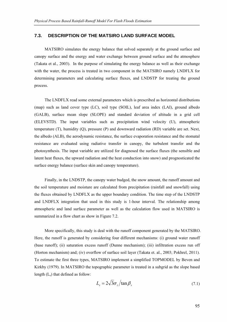
Physical Process Based Rainfall-Runoff Model For Flash Floods Estimation
95
7.3. DESCRIPTION OF THE MATSIRO LAND SURFACE MODEL
MATSIRO simulates the energy balance that solved separately at the ground surface and
canopy surface and the energy and water exchange between ground surface and the atmosphere
(Takata et al., 2003). In the purpose of simulating the energy balance as well as their exchange
with the water, the process is treated in two component in the MATSIRO namely LNDFLX for
determining parameters and calculating surface fluxes, and LNDSTP for treating the ground
process.
The LNDFLX read some external parameters which is prescribed as horizontal distributions
(map) such as land cover type (LC), soil type (SOIL), leaf area index (LAI), ground albedo
(GALB), surface mean slope (SLOPE) and standard deviation of altitude in a grid cell
(ELEVSTD). The input variables such as precipitation wind velocity (U), atmospheric
temperature (T), humidity (Q), pressure (P) and downward radiation (RD) variable are set. Next,
the albedo (ALB), the aerodynamic resistance, the surface evaporation resistance and the stomatal
resistance are evaluated using radiative transfer in canopy, the turbulent transfer and the
photosynthesis. The input variable are utilized for diagnosed the surface fluxes (the sensible and
latent heat fluxes, the upward radiation and the heat conduction into snow) and prognosticated the
surface energy balance (surface skin and canopy temperature).
Finally, in the LNDSTP, the canopy water budged, the snow amount, the runoff amount and
the soil temperature and moisture are calculated from precipitation (rainfall and snowfall) using
the fluxes obtained by LNDFLX as the upper boundary condition. The time step of the LNDSTP
and LNDFLX integration that used in this study is 1-hour interval. The relationship among
atmospheric and land surface parameter as well as the calculation flow used in MATSIRO is
summarized in a flow chart as show in Figure 7.2.
More specifically, this study is deal with the runoff component generated by the MATSIRO.
Here, the runoff is generated by considering four different mechanisms: (i) ground water runoff
(base runoff); (ii) saturation excess runoff (Dunne mechanism); (iii) infiltration excess run off
(Horton mechanism) and; (iv) overflow of surface soil layer (Takata et. al., 2003; Pokhrel, 2011).
To estimate the first three types, MATSIRO implement a simplified TOPMODEL by Beven and
Kirkby (1979). In MATSIRO the topographic parameter is treated in a subgrid as the slope based
length (Ls) that defined as follow:
szsL βσ tan32= (7.1)
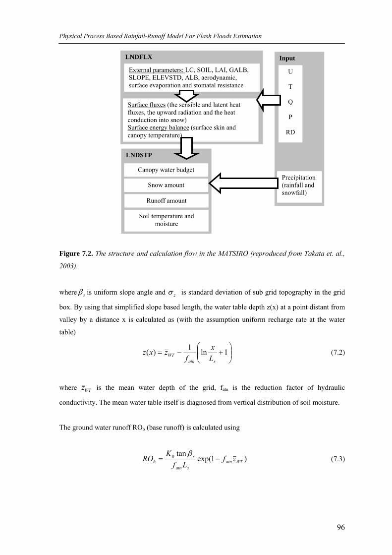
Physical Process Based Rainfall-Runoff Model For Flash Floods Estimation
96
Figure 7.2. The structure and calculation flow in the MATSIRO (reproduced from Takata et. al.,
2003).
where sβ is uniform slope angle and zσ is standard deviation of sub grid topography in the grid
box. By using that simplified slope based length, the water table depth z(x) at a point distant from
valley by a distance x is calculated as (with the assumption uniform recharge rate at the water
table)
⎟⎟⎠
⎞⎜⎜⎝
⎛+−= 1ln1)(
satnWT L
xf
zxz (7.2)
where WTz is the mean water depth of the grid, fatn is the reduction factor of hydraulic
conductivity. The mean water table itself is diagnosed from vertical distribution of soil moisture.
The ground water runoff ROb (base runoff) is calculated using
)1exp(tan0
WTatnsatn
sb zf
LfK
RO −=β
(7.3)
LNDFLX
External parameters: LC, SOIL, LAI, GALB, SLOPE, ELEVSTD, ALB, aerodynamic, surface evaporation and stomatal resistance
Surface fluxes (the sensible and latent heat fluxes, the upward radiation and the heat conduction into snow) Surface energy balance (surface skin and canopy temperature)
LNDSTP
Canopy water budget
Snow amount
Runoff amount
Soil temperature and moisture
Input
U
T
Q
P
RD
Precipitation (rainfall and snowfall)
Physical Process Based Rainfall-Runoff Model For Flash Floods Estimation
97
where K0 is saturation hydraulic conductivity at the surface. Here it assumed that the base runoff
is equal to recharge. A quasi equilibrium assumption i.e. groundwater runoff at a point in a slope
is equal to accumulated groundwater recharge in the upper area. By this assumption a concept of
saturated area fraction (Asat) is introduced. In the low topographic condition such as lower part of
slope, the water table depth becomes shallower and reaches ground surface, therefore runoff is
generated. Asat is expressed as:
)1exp(1 −−= WTatnsat zfA (7.4)
In the saturation excess runoff, ROs is assigned as the runoff produced by precipitation over the
saturated area around the river channel, at it is estimated as (Pokhrel, 2011):
satlcs ARO )Pr(Pr **** += (7.5)
where **Prc and **Prl are the effective convective precipitation after interception loss and
effective stratiform precipitation after interception loss respectively.
Infiltration excess runoff occurred when the rainfall intensity exceeds the infiltration
capacity of the soil (Beven and Kirkby, 1979). In the MATSIRO the infiltration capacity is
assumed equal to saturated hydraulic conductivity. The infiltration excess run off, ROi, is
calculated separately for convective and statiform rainfall by considering their proportion in the
grid as follow (Pokhrel, 2011):
)1)(Pr/max(Pr 0****
satlccci AKARO −−+=
)1)(max(Pr 0**
satlnci AKRO −−= (7.6)
ncic
cici ROAROARO )1( −+=
where, ciRO is infiltration excess runoff in areas with convective precipitation; nc
iRO is
infiltration excess runoff in areas with stratiform precipitation; iRO is total infiltration excess
runoff; Ac is fraction f grid area over which precipitation input is convective (default is 10 in
MATSIRO).
Finally overflow of surface soil layer ROo is calculated, which is occurs when moisture
flux input to the surface soil layer is higher that its conductivity or if soil layer is oversaturated in
the numerical solution, which not theoretically possible (Pokhrel, 2011). ROo is calculated as:
Physical Process Based Rainfall-Runoff Model For Flash Floods Estimation
98
Lgwstrsato tzwwwRO ΔΔ−−= /)max( ρ (7.7)
where w is moisture content of the surface soil layer, wsat is soil moisture capacity (porosity) of
the surface soil layer; wstr is surface storage capacity, wρ is density of the water, gzΔ is thickness
of the surface soil layer and LtΔ is calculation time step.
The produced runoff then routes through river network by using Total Runoff Integration
Pathways (TRIP) (Oki et al., 1998). By this process a river flow accumulation is generated for
every time steps, therefore the estimated river flow (discharge) can be observed in any position in
the region, particularly in the outlet of the catchment.
7.4. METHOD
7.4.1. DEM processing for the topographic and river network parameters extraction.
As previously explained that MATSIRO uses some topographical parameter such as
surface slope and standard deviation of altitude in a grid cell. Those parameters are extracted from
DEM analysis of SRTM-DEM data. Suppose the surface function of DEM is defined as z=f(x,y),
where x and y is the grid location of the elevation z. The first derivative in x and y direction is
respectively defined as fx=df/dx and fy=df/dy. The slope angle is calculated by following
formula:
⎟⎠⎞⎜
⎝⎛ += 22tan yxs ffArcβ (7.8)
The standard deviation of subgrid topography in the grid box is calculated using standard
deviation function during aggregation process from 90m×90m into 1km×1km grid size.
Another contribution of SRTM-DEM information into MATSIRO is related to runoff
routing processes that made possible by implementing the Total Runoff Integration Pathways
(TRIP) (Oki et al, 1998). TRIP is a river channel network that shows the lateral water movement
overland following the path of the river channels. TRIP is determined by implementing flow
direction calculation procedure DEM. Since the original TRIP was prepared for global scale
(1°×1°), therefore to fulfill the study purpose that need more detailed data, the flow direction
calculation procedure is performed to the SRTM DEM. This calculation process to derived flow
directions and flow accumulation map was facilitated by Integrated Land and Water Information
System (ILWIS) (Maathuis and Wang, 2008).
Physical Process Based Rainfall-Runoff Model For Flash Floods Estimation
99
7.4.2. Land surface parameters data handling
MODIS data has been utilized for acquiring land surface parameters in MATSIRO. There
are several MODIS-based data products that are relevant as the MATSIRO data input such as
Leaf Area Index (MCD15A3), surface albedo (MCD43B3) and Land cover type (MCD12Q1).
Since those of data are mainly delivered in Hierarchical Data Format (HDF) which is not
compatible with the MATSIRO, data format conversion had been conducted. The principle of the
conversion was made the data became raw binary format, which is flexible to convert into another
data type. The HDF was converted into raw binary format by using HEG tool. The HEG tool is a
Java application to convert HDF Earth Observation System (HDF-EOS) to Geographic
Information System (GIS) format such as GeoTIFF, native (or raw) binary format, and HDF-EOS
grid format. The conversion of raw binary format to MATSIRO data input format had been
facilitated by the GTOOL.
MATSIRO uses soil texture as the primary key to store some physical properties of soil
such as soil heat capacity, soil heat conductivity, porosity, saturation hydraulic conductivity,
saturation hydraulic potential and exponent parameter of moisture retention curve (Takata et al,
2003). Here, the texture soil map had been obtained from Digital Soil Map of The World. This is
a vector data set that is prepared based on the FAO-UNESCO soil map of the world at 1:
5,000,000 scales.
7.4.3. Atmospheric data forcing preparation and statistical downscaling
Several atmospheric data forcing for MATSIRO such as precipitation, wind velocity,
atmospheric temperature, atmospheric humidity, atmospheric pressure, downward radiation
(infrared and visible), and cloud coverage had been acquired from various data sources.
Precipitation, wind velocity, atmospheric temperature, atmospheric humidity and atmospheric
pressure are acquired from AMeDAS observation network. Those of data had been prepared by
conducting spatial interpolation of the corresponding value based on the observation point
location. The longwave and shortwave downward radiation (infrared and visible) was derived
from CERES sensors.
The rainfall data forcing, specifically during June to September 2010 period, was derived
by estimating from MTSAT data. A statistical model by utilizing the MTSAT 10.8 µm channel
data had been implemented for estimating rainfall. A cloud type classification based on MTSAT
split window had also been developed and implemented for the purpose of Cumulonimbus (Cb)
cloud detection (Suseno and Yamada, 2012b). The atmospheric environmental conditions i.e.
Physical Process Based Rainfall-Runoff Model For Flash Floods Estimation
100
atmospheric vertical instability and the availability of precipitable water vapor that sustain the Cb
cloud generation had been taken into account during rainfall estimation process. Particularly for
the convective rain, the statistical model had been combined with precipitable water and
atmospheric vertical instability. Since the estimated rainfall output was preserving the native
resolution of MTSAT image (approximately 5 km grid), a statistical downscaling method was
conducted to convert the data into 1 km grid size. Here the estimated rainfall by MTSAT satellite
is downscaled with the observed rainfall (MTSAT downscaled hereinafter).
The downscaling process aims to combine the advantage of those two rainfall data capture
systems. Rain gauge observation is the only source of rainfall data that is obtained through direct
measurement, however it has limitation due to lack of distribution particularly for remote area.
Satellite observation is indirect measurement in nature, but it has very good spatial coverage. By
merging the benefit of those systems, the combined result is expected to be improved in accuracy,
coverage and resolution (Vila et al, 2009). The discrepancy between satellite based rainfall
estimation and direct observation by rain gauge should be reduced during downscaling process
through bias correction. The bias correction is based on: (i) additive; and (ii) multiplicative
method which is applied for each station in hourly basis. The additive bias correction ( +rr ) and
multiplicative bias correction ( *rr ) are respectively defined in equation 7.9 and 7.10 as following
(Vila et al, 2009):
)( isat
iobssat rrrrrrrr −+=+ (7.9)
⎟⎟⎠
⎞⎜⎜⎝
⎛×= i
sat
iobs
sat rrrrrrrr*
(7.10)
The first term in both equations is satellite based rainfall estimation. The second term in equation
7.9 and 7.10 represent respectively the mean bias (represented by the bar) both additive bias and
multiplicative bias between the observed and estimated rainfall for each station (denoted by
superscript i). The procedure of performing statistical downscaling is as following. The observed
rainfall is interpolated using inverse distance weight method in 1-km grid size, with the limiting
distance about 10 km. The satellite based rainfall is disaggregated from 5-km into 1-km grid
resolution. Next, the difference between additive or multiplicative was calculated. The mean of
both additive bias and multiplicative bias for each station was performed by applying 3×3
summation filter, divided by number of grid containing bias value. The downscaled bias corrected
rainfall was calculated using equation 3 and 4 for the additive and multiplicative accordingly. One
particular bias correction method was selected for each point grid based on the minimum
difference between that bias corrected rainfall and observed rainfall. For the grid point outside the
limiting distance of interpolation, the original estimated rainfall was assigned.
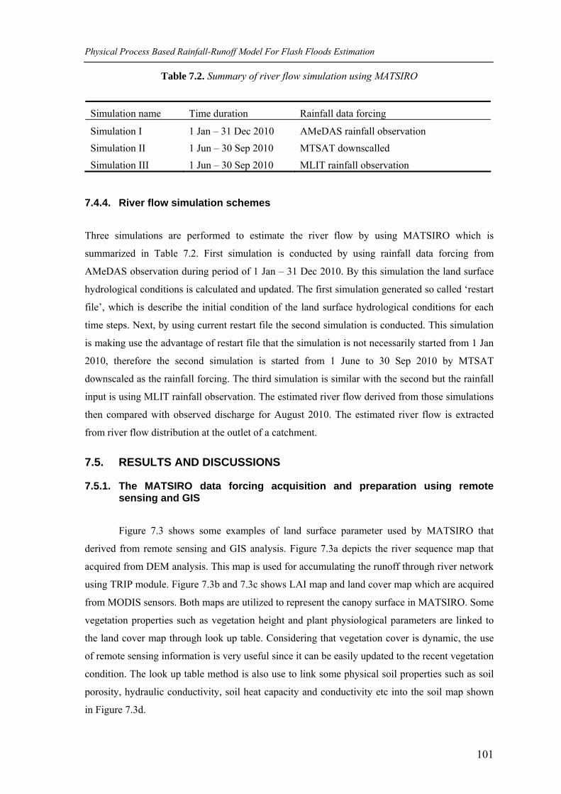
Physical Process Based Rainfall-Runoff Model For Flash Floods Estimation
101
Table 7.2. Summary of river flow simulation using MATSIRO
Simulation name Time duration Rainfall data forcing
Simulation I 1 Jan – 31 Dec 2010 AMeDAS rainfall observation Simulation II 1 Jun – 30 Sep 2010 MTSAT downscalled Simulation III 1 Jun – 30 Sep 2010 MLIT rainfall observation
7.4.4. River flow simulation schemes
Three simulations are performed to estimate the river flow by using MATSIRO which is
summarized in Table 7.2. First simulation is conducted by using rainfall data forcing from
AMeDAS observation during period of 1 Jan – 31 Dec 2010. By this simulation the land surface
hydrological conditions is calculated and updated. The first simulation generated so called ‘restart
file’, which is describe the initial condition of the land surface hydrological conditions for each
time steps. Next, by using current restart file the second simulation is conducted. This simulation
is making use the advantage of restart file that the simulation is not necessarily started from 1 Jan
2010, therefore the second simulation is started from 1 June to 30 Sep 2010 by MTSAT
downscaled as the rainfall forcing. The third simulation is similar with the second but the rainfall
input is using MLIT rainfall observation. The estimated river flow derived from those simulations
then compared with observed discharge for August 2010. The estimated river flow is extracted
from river flow distribution at the outlet of a catchment.
7.5. RESULTS AND DISCUSSIONS
7.5.1. The MATSIRO data forcing acquisition and preparation using remote sensing and GIS
Figure 7.3 shows some examples of land surface parameter used by MATSIRO that
derived from remote sensing and GIS analysis. Figure 7.3a depicts the river sequence map that
acquired from DEM analysis. This map is used for accumulating the runoff through river network
using TRIP module. Figure 7.3b and 7.3c shows LAI map and land cover map which are acquired
from MODIS sensors. Both maps are utilized to represent the canopy surface in MATSIRO. Some
vegetation properties such as vegetation height and plant physiological parameters are linked to
the land cover map through look up table. Considering that vegetation cover is dynamic, the use
of remote sensing information is very useful since it can be easily updated to the recent vegetation
condition. The look up table method is also use to link some physical soil properties such as soil
porosity, hydraulic conductivity, soil heat capacity and conductivity etc into the soil map shown
in Figure 7.3d.
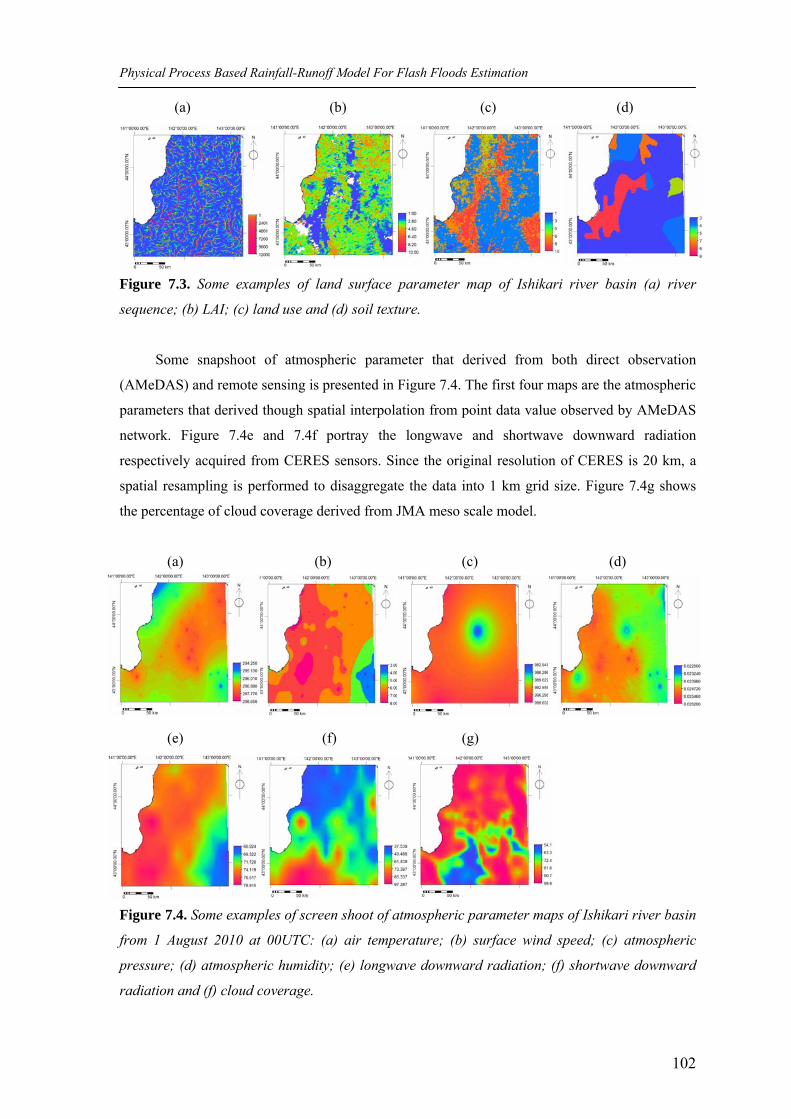
Physical Process Based Rainfall-Runoff Model For Flash Floods Estimation
102
(a) (b) (c) (d)
Figure 7.3. Some examples of land surface parameter map of Ishikari river basin (a) river
sequence; (b) LAI; (c) land use and (d) soil texture.
Some snapshoot of atmospheric parameter that derived from both direct observation
(AMeDAS) and remote sensing is presented in Figure 7.4. The first four maps are the atmospheric
parameters that derived though spatial interpolation from point data value observed by AMeDAS
network. Figure 7.4e and 7.4f portray the longwave and shortwave downward radiation
respectively acquired from CERES sensors. Since the original resolution of CERES is 20 km, a
spatial resampling is performed to disaggregate the data into 1 km grid size. Figure 7.4g shows
the percentage of cloud coverage derived from JMA meso scale model.
(a) (b) (c) (d)
(e) (f) (g)
Figure 7.4. Some examples of screen shoot of atmospheric parameter maps of Ishikari river basin
from 1 August 2010 at 00UTC: (a) air temperature; (b) surface wind speed; (c) atmospheric
pressure; (d) atmospheric humidity; (e) longwave downward radiation; (f) shortwave downward
radiation and (f) cloud coverage.
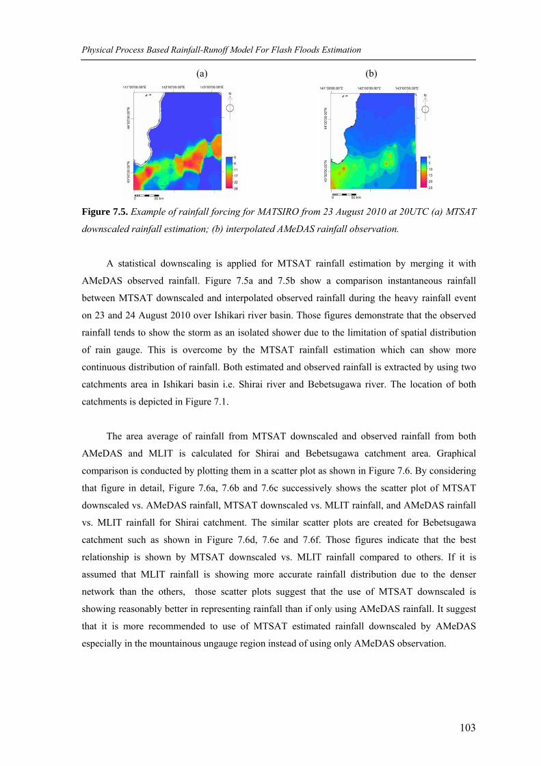
Physical Process Based Rainfall-Runoff Model For Flash Floods Estimation
103
(a) (b)
Figure 7.5. Example of rainfall forcing for MATSIRO from 23 August 2010 at 20UTC (a) MTSAT
downscaled rainfall estimation; (b) interpolated AMeDAS rainfall observation.
A statistical downscaling is applied for MTSAT rainfall estimation by merging it with
AMeDAS observed rainfall. Figure 7.5a and 7.5b show a comparison instantaneous rainfall
between MTSAT downscaled and interpolated observed rainfall during the heavy rainfall event
on 23 and 24 August 2010 over Ishikari river basin. Those figures demonstrate that the observed
rainfall tends to show the storm as an isolated shower due to the limitation of spatial distribution
of rain gauge. This is overcome by the MTSAT rainfall estimation which can show more
continuous distribution of rainfall. Both estimated and observed rainfall is extracted by using two
catchments area in Ishikari basin i.e. Shirai river and Bebetsugawa river. The location of both
catchments is depicted in Figure 7.1.
The area average of rainfall from MTSAT downscaled and observed rainfall from both
AMeDAS and MLIT is calculated for Shirai and Bebetsugawa catchment area. Graphical
comparison is conducted by plotting them in a scatter plot as shown in Figure 7.6. By considering
that figure in detail, Figure 7.6a, 7.6b and 7.6c successively shows the scatter plot of MTSAT
downscaled vs. AMeDAS rainfall, MTSAT downscaled vs. MLIT rainfall, and AMeDAS rainfall
vs. MLIT rainfall for Shirai catchment. The similar scatter plots are created for Bebetsugawa
catchment such as shown in Figure 7.6d, 7.6e and 7.6f. Those figures indicate that the best
relationship is shown by MTSAT downscaled vs. MLIT rainfall compared to others. If it is
assumed that MLIT rainfall is showing more accurate rainfall distribution due to the denser
network than the others, those scatter plots suggest that the use of MTSAT downscaled is
showing reasonably better in representing rainfall than if only using AMeDAS rainfall. It suggest
that it is more recommended to use of MTSAT estimated rainfall downscaled by AMeDAS
especially in the mountainous ungauge region instead of using only AMeDAS observation.
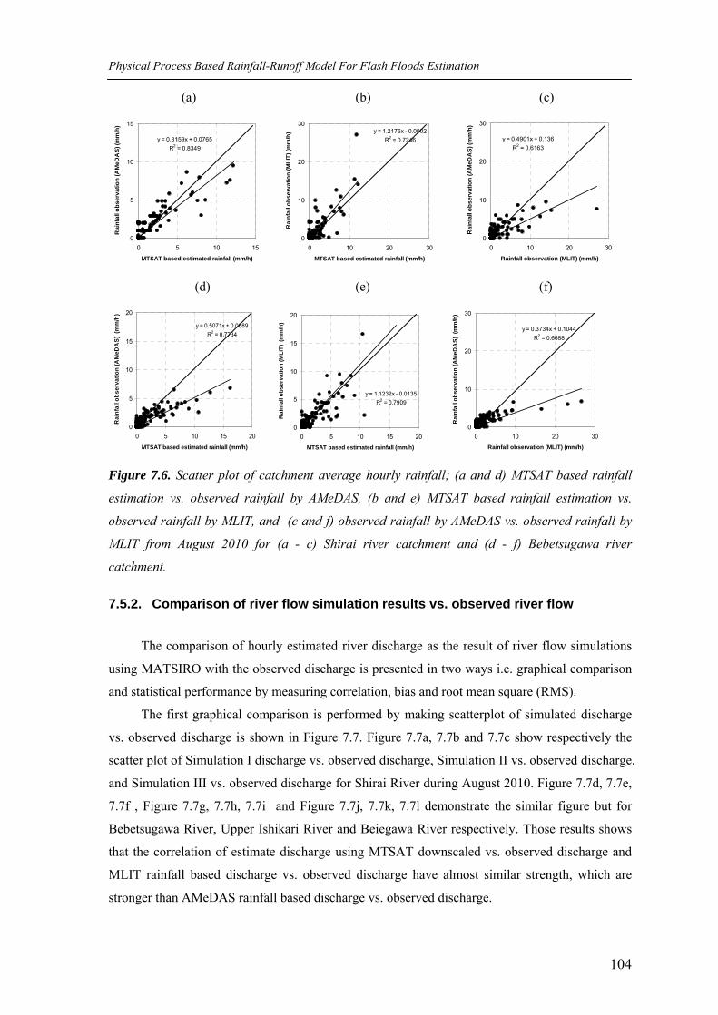
Physical Process Based Rainfall-Runoff Model For Flash Floods Estimation
104
(a) (b) (c)
y = 0.8159x + 0.0765R2 = 0.8349
0
5
10
15
0 5 10 15
MTSAT based estimated rainfall (mm/h)
Rai
nfal
l obs
erva
tion
(AM
eDA
S) (m
m/h
)
y = 1.2176x - 0.0002R2 = 0.7246
0
10
20
30
0 10 20 30
MTSAT based estimated rainfall (mm/h)
Rai
nfal
l obs
erva
tion
(MLI
T) (m
m/h
)
y = 0.4901x + 0.136R2 = 0.6163
0
10
20
30
0 10 20 30
Rainfall observation (MLIT) (mm/h)
Rai
nfal
l obs
erva
tion
(AM
eDA
S) (m
m/h
)
(d) (e) (f)
y = 0.5071x + 0.0689R2 = 0.7734
0
5
10
15
20
0 5 10 15 20
MTSAT based estimated rainfall (mm/h)
Rai
nfal
l obs
erva
tion
(AM
eDA
S) (
mm
/h)
y = 1.1232x - 0.0135R2 = 0.7909
0
5
10
15
20
0 5 10 15 20
MTSAT based estimated rainfall (mm/h)
Rai
nfal
l obs
erva
tion
(MLI
T) (
mm
/h)
y = 0.3734x + 0.1044R2 = 0.6688
0
10
20
30
0 10 20 30
Rainfall observation (MLIT) (mm/h)R
ainf
all o
bser
vatio
n (A
MeD
AS)
(m
m/h
)
Figure 7.6. Scatter plot of catchment average hourly rainfall; (a and d) MTSAT based rainfall
estimation vs. observed rainfall by AMeDAS, (b and e) MTSAT based rainfall estimation vs.
observed rainfall by MLIT, and (c and f) observed rainfall by AMeDAS vs. observed rainfall by
MLIT from August 2010 for (a - c) Shirai river catchment and (d - f) Bebetsugawa river
catchment.
7.5.2. Comparison of river flow simulation results vs. observed river flow
The comparison of hourly estimated river discharge as the result of river flow simulations
using MATSIRO with the observed discharge is presented in two ways i.e. graphical comparison
and statistical performance by measuring correlation, bias and root mean square (RMS).
The first graphical comparison is performed by making scatterplot of simulated discharge
vs. observed discharge is shown in Figure 7.7. Figure 7.7a, 7.7b and 7.7c show respectively the
scatter plot of Simulation I discharge vs. observed discharge, Simulation II vs. observed discharge,
and Simulation III vs. observed discharge for Shirai River during August 2010. Figure 7.7d, 7.7e,
7.7f , Figure 7.7g, 7.7h, 7.7i and Figure 7.7j, 7.7k, 7.7l demonstrate the similar figure but for
Bebetsugawa River, Upper Ishikari River and Beiegawa River respectively. Those results shows
that the correlation of estimate discharge using MTSAT downscaled vs. observed discharge and
MLIT rainfall based discharge vs. observed discharge have almost similar strength, which are
stronger than AMeDAS rainfall based discharge vs. observed discharge.
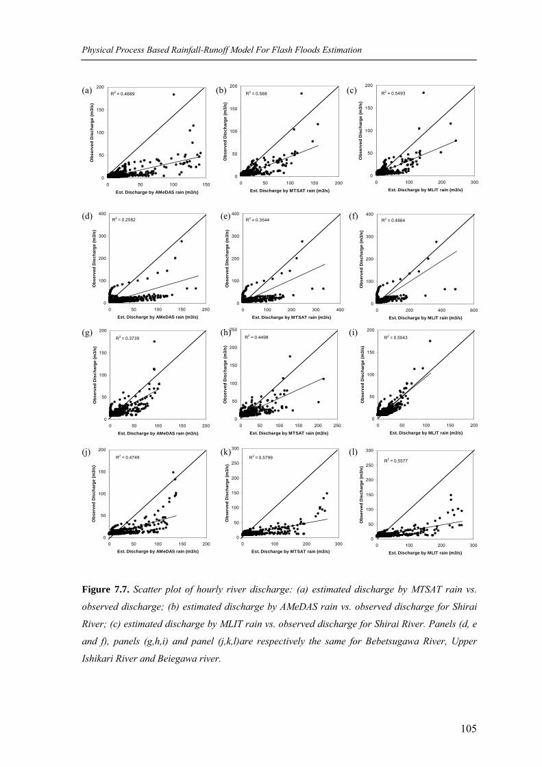
Physical Process Based Rainfall-Runoff Model For Flash Floods Estimation
105
R2 = 0.568
0
50
100
150
200
0 50 100 150 200
Est. Discharge by MTSAT rain (m3/s)
Obs
erve
d D
isch
arge
(m3/
s)
R2 = 0.4689
0
50
100
150
200
0 50 100 150
Est. Discharge by AMeDAS rain (m3/s)
Obs
erve
d D
isch
arge
(m3/
s)R2 = 0.5493
0
50
100
150
200
0 100 200 300
Est. Discharge by MLIT rain (m3/s)
Obs
erve
d D
isch
arge
(m3/
s)
R2 = 0.3544
0
100
200
300
400
0 100 200 300 400
Est. Discharge by MTSAT rain (m3/s)
Obs
erve
d D
isch
arge
(m3/
s)R2 = 0.2582
0
100
200
300
400
0 50 100 150 200
Est. Discharge by AMeDAS rain (m3/s)
Obs
erve
d D
isch
arge
(m3/
s)
R2 = 0.4864
0
100
200
300
400
0 200 400 600
Est. Discharge by MLIT rain (m3/s)
Obs
erve
d D
isch
arge
(m3/
s)
R2 = 0.4498
0
50
100
150
200
250
0 50 100 150 200 250
Est. Discharge by MTSAT rain (m3/s)
Obs
erve
d D
isch
arge
(m3/
s)
R2 = 0.3739
0
50
100
150
200
0 50 100 150 200
Est. Discharge by AMeDAS rain (m3/s)
Obs
erve
d D
isch
arge
(m3/
s)
R2 = 0.5043
0
50
100
150
200
0 50 100 150 200
Est. Discharge by MLIT rain (m3/s)
Obs
erve
d D
isch
arge
(m3/
s)
R2 = 0.5799
0
50
100
150
200
250
300
0 100 200 300
Est. Discharge by MTSAT rain (m3/s)
Obs
erve
d D
isch
arge
(m3/
s)
R2 = 0.4749
0
50
100
150
200
0 50 100 150 200
Est. Discharge by AMeDAS rain (m3/s)
Obs
erve
d D
isch
arge
(m3/
s)
R2 = 0.5577
0
50
100
150
200
250
300
0 100 200 300
Est. Discharge by MLIT rain (m3/s)
Obs
erve
d D
isch
arge
(m3/
s)
(a) (b) (c)
(d) (e) (f)
(g) (h) (i)
(j) (k) (l)
Figure 7.7. Scatter plot of hourly river discharge: (a) estimated discharge by MTSAT rain vs.
observed discharge; (b) estimated discharge by AMeDAS rain vs. observed discharge for Shirai
River; (c) estimated discharge by MLIT rain vs. observed discharge for Shirai River. Panels (d, e
and f), panels (g,h,i) and panel (j,k,l)are respectively the same for Bebetsugawa River, Upper
Ishikari River and Beiegawa river.

Physical Process Based Rainfall-Runoff Model For Flash Floods Estimation
106
This result suggest that the use of MTSAT downscaled as rainfall forcing in MATSIRO is more
recommended than that the use of AMeDAS rainfall data forcing.
The second graphical comparisons between simulated discharge vs. observed discharge
are shown as line graph in Figure 7.8a to 7.8d which represent the comparison result for Shirai
river, Upper Ishikari River, Beiegawa River respectively and Bebetsugawa River respectively.
From those graphical comparison it clearly shows that the simulated discharge are mostly
overestimated. However, to show more clearly about the river flow simulation during flash flood
event, Figure 7.9a to 7.9d shows the comparison peak discharge hydrograph during heavy rainfall
event from 23 and 24 August 2010 for Shirai River, Upper Ishikari River, Beiegawa River
respectively and Bebetsugawa River respectively. These flood events are considered as flash flood
due to short time to peak discharge and relatively high peak discharge. The river flow simulations
results demonstrate that estimated discharge using MLIT rainfall is the best for predicting peak
discharge compared with the others, especially in Shirai River and Bebetsugawa river. This is
readily explained due to MLIT has relatively dense rainfall network compared with AMeDAS,
therefore they can represent rainfall distribution better than others. The second best is shown by
estimated discharge using MTSAT downscaled and the last is by estimated discharge using
AMeDAS rainfall. This result actually is consistent with the previous result, therefore for
providing flash flood information in ungauged catchment the use of MTSAT downscaled as
rainfall forcing is better than only the use of AMeDAS rainfall. When it is assumed that the sparse
distribution of rainfall network is common situation in many places, the MTSAT downscaled
demonstrate more advantage as input forcing in a physically based model than if only using the
interpolated sparse rainfall observation. It is because MTSAT is basically good in representing
rainfall distribution, but less accurate in predicting its amount. This limitation then improved by
conducting bias adjustment using observed rainfall even though they are acquired using sparse
station distribution.
The above mentioned graphical comparison then confirmed by statistical performance
calculation result such as shown by Table 7.3. From the bold-faced numbers that show the best
statistic suggests that the simulated discharge using MTSAT downscaled is reasonably
comparable with the MLIT rainfall based simulated discharge and they are much better than the
use of only AMeDAS rainfall as input forcing. This statistical performance results confirm that
the use of MTSAT downscaled as rainfall forcing in MATSIRO is more recommended than that
the use of AMeDAS rainfall data forcing.
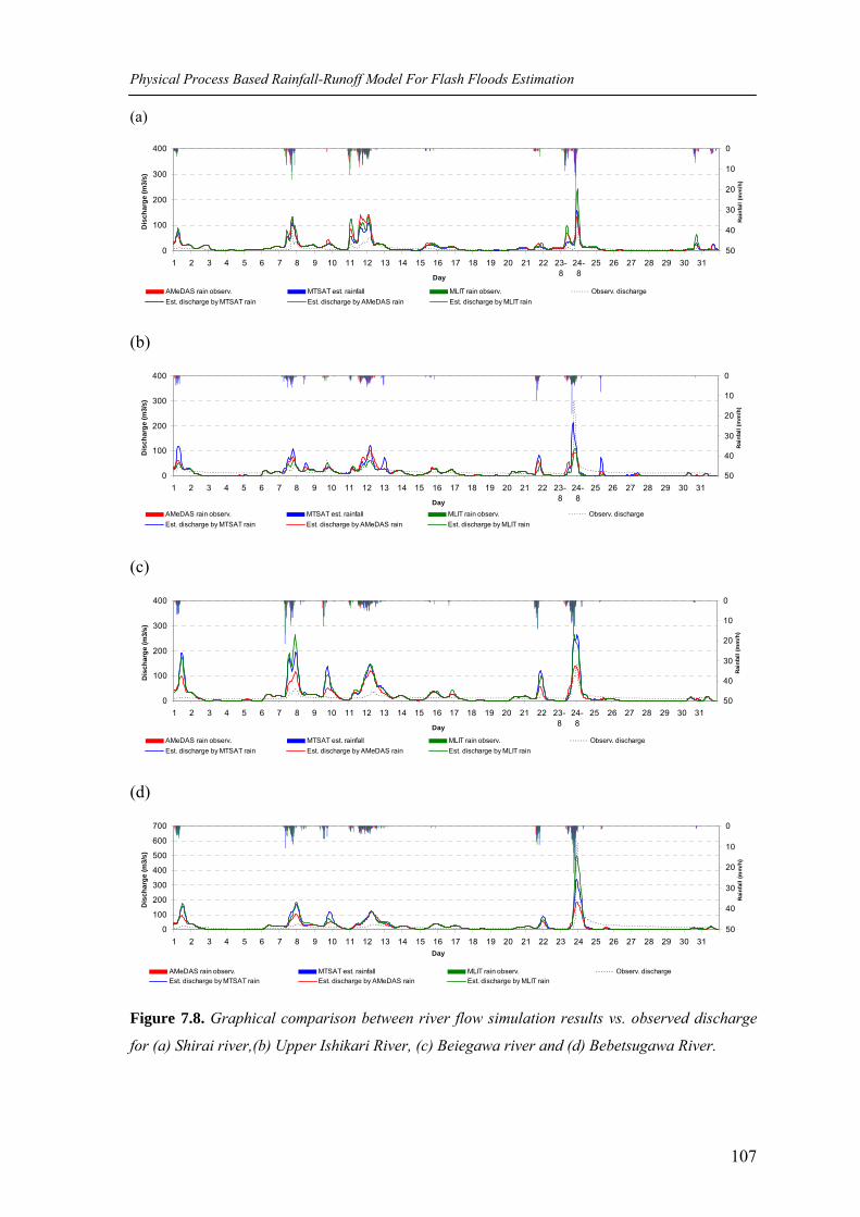
Physical Process Based Rainfall-Runoff Model For Flash Floods Estimation
107
(a)
0
100
200
300
400
1 2 3 4 5 6 7 8 9 10 11 12 13 14 15 16 17 18 19 20 21 22 23-8
24-8
25 26 27 28 29 30 31
Day
Dis
char
ge (m
3/s)
0
10
20
30
40
50
Rain
fall
(mm
/h)
AMeDAS rain observ. MTSAT est. rainfall MLIT rain observ. Observ. dischargeEst. discharge by MTSAT rain Est. discharge by AMeDAS rain Est. discharge by MLIT rain
(b)
0
100
200
300
400
1 2 3 4 5 6 7 8 9 10 11 12 13 14 15 16 17 18 19 20 21 22 23-8
24-8
25 26 27 28 29 30 31
Day
Dis
char
ge (m
3/s)
0
10
20
30
40
50
Rain
fall
(mm
/h)
AMeDAS rain observ. MTSAT est. rainfall MLIT rain observ. Observ. dischargeEst. discharge by MTSAT rain Est. discharge by AMeDAS rain Est. discharge by MLIT rain
(c)
0
100
200
300
400
1 2 3 4 5 6 7 8 9 10 11 12 13 14 15 16 17 18 19 20 21 22 23-8
24-8
25 26 27 28 29 30 31
Day
Dis
char
ge (m
3/s)
0
10
20
30
40
50
Rain
fall
(mm
/h)
AMeDAS rain observ. MTSAT est. rainfall MLIT rain observ. Observ. dischargeEst. discharge by MTSAT rain Est. discharge by AMeDAS rain Est. discharge by MLIT rain
(d)
0
100
200
300
400
500
600
700
1 2 3 4 5 6 7 8 9 10 11 12 13 14 15 16 17 18 19 20 21 22 23 24 25 26 27 28 29 30 31Day
Dis
char
ge (m
3/s)
0
10
20
30
40
50
Rain
fall
(mm
/h)
AMeDAS rain observ. MTSAT est. rainfall MLIT rain observ. Observ. dischargeEst. discharge by MTSAT rain Est. discharge by AMeDAS rain Est. discharge by MLIT rain
Figure 7.8. Graphical comparison between river flow simulation results vs. observed discharge
for (a) Shirai river,(b) Upper Ishikari River, (c) Beiegawa river and (d) Bebetsugawa River.
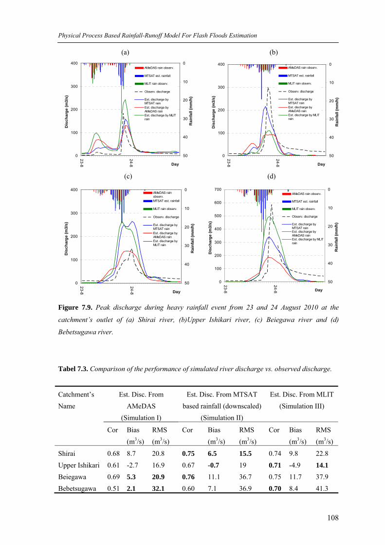
Physical Process Based Rainfall-Runoff Model For Flash Floods Estimation
108
0
100
200
300
400
23-8
24-8 Day
Dis
char
ge (m
3/s)
0
10
20
30
40
50
Rai
nfal
l (m
m/h
)
AMeDAS rain observ.
MTSAT est. rainfall
MLIT rain observ.
Observ. discharge
Est. discharge byMTSAT rainEst. discharge byAMeDAS rainEst. discharge by MLITrain
0
100
200
300
400
500
600
700
23-8
24-8 Day
Dis
char
ge (m
3/s)
0
10
20
30
40
50
Rai
nfal
l (m
m/h
)
AMeDAS rain observ.
MTSAT est. rainfall
MLIT rain observ.
Observ. discharge
Est. discharge byMTSAT rainEst. discharge byAMeDAS rainEst. discharge by MLITrain
0
100
200
300
400
23-8
24-8 Day
Dis
char
ge (m
3/s)
0
10
20
30
40
50
Rai
nfal
l (m
m/h
)
AMeDAS rain observ.
MTSAT est. rainfall
MLIT rain observ.
Observ. discharge
Est. discharge byMTSAT rainEst. discharge byAMeDAS rainEst. discharge by MLITrain
0
100
200
300
400
23-8
24-8 Day
Dis
char
ge (m
3/s)
0
10
20
30
40
50
Rai
nfal
l (m
m/h
)AMeDAS rainobserv.MTSAT est. rainfall
MLIT rain observ.
Observ. discharge
Est. discharge byMTSAT rainEst. discharge byAMeDAS rainEst. discharge byMLIT rain
(a) (b)
(c) (d)
Figure 7.9. Peak discharge during heavy rainfall event from 23 and 24 August 2010 at the
catchment’s outlet of (a) Shirai river, (b)Upper Ishikari river, (c) Beiegawa river and (d)
Bebetsugawa river.
Tabel 7.3. Comparison of the performance of simulated river discharge vs. observed discharge.
Est. Disc. From AMeDAS
(Simulation I)
Est. Disc. From MTSAT based rainfall (downscaled)
(Simulation II)
Est. Disc. From MLIT (Simulation III)
Catchment’s Name
Cor Bias (m3/s)
RMS (m3/s)
Cor Bias (m3/s)
RMS (m3/s)
Cor Bias (m3/s)
RMS (m3/s)
Shirai 0.68 8.7 20.8 0.75 6.5 15.5 0.74 9.8 22.8 Upper Ishikari 0.61 -2.7 16.9 0.67 -0.7 19 0.71 -4.9 14.1 Beiegawa 0.69 5.3 20.9 0.76 11.1 36.7 0.75 11.7 37.9 Bebetsugawa 0.51 2.1 32.1 0.60 7.1 36.9 0.70 8.4 41.3
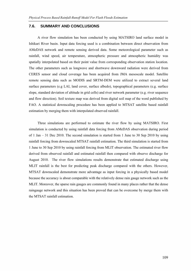
Physical Process Based Rainfall-Runoff Model For Flash Floods Estimation
109
7.6. SUMMARY AND CONCLUSIONS
A river flow simulation has been conducted by using MATSIRO land surface model in
Ishikari River basin. Input data forcing used is a combination between direct observation from
AMeDAS network and remote sensing derived data. Some meteorological parameter such as
rainfall, wind speed, air temperature, atmospheric pressure and atmospheric humidity was
spatially interpolated based on their point value from corresponding observation station location.
The other parameters such as longwave and shortwave downward radiation were derived from
CERES sensor and cloud coverage has been acquired from JMA mesoscale model. Satellite
remote sensing data such as MODIS and SRTM-DEM were utilized to extract several land
surface parameters (e.g LAI, land cover, surface albedo), topographical parameters (e.g. surface
slope, standard deviation of altitude in grid cells) and river network parameter (e.g. river sequence
and flow direction). Soil texture map was derived from digital soil map of the word published by
FAO. A statistical downscaling procedure has been applied to MTSAT satellite based rainfall
estimation by merging them with interpolated observed rainfall.
Three simulations are performed to estimate the river flow by using MATSIRO. First
simulation is conducted by using rainfall data forcing from AMeDAS observation during period
of 1 Jan – 31 Dec 2010. The second simulation is started from 1 June to 30 Sep 2010 by using
rainfall forcing from downscaled MTSAT rainfall estimation. The third simulation is started from
1 June to 30 Sep 2010 by using rainfall forcing from MLIT observation. The estimated river flow
derived from observed rainfall and estimated rainfall then compared with observe discharge for
August 2010. The river flow simulations results demonstrate that estimated discharge using
MLIT rainfall is the best for predicting peak discharge compared with the others. However,
MTSAT downscaled demonstrate more advantage as input forcing in a physically based model
because the accuracy is about comparable with the relatively dense rain gauge network such as the
MLIT. Moreover, the sparse rain gauges are commonly found in many places rather that the dense
raingauge network and this situation has been proved that can be overcome by merge them with
the MTSAT rainfall estimation.

Chapter 8. SUMMARY, CONCLUSIONS AND RECOMMENDATIONS
Summary, Conclusions and Recommendation
111
8.1. SUMMARY AND CONCLUSIONS
This chapter introduces the main results and conclusions which are drawn in relation to
the key objectives of this study. They are summarized as following:
Key objective 1: To develop and evaluate the geostationary satellite based rainfall estimation by
considering not only cloud top temperature but also cloud type (i.e. Cb cloud type) and
atmospheric environmental conditions sustaining the convective cloud development (i.e.
precipitable water vapor and atmospheric vertical instability).
The basic approach of rainfall estimation using geostationary satellite.
In this chapter, the main approach of geostationary satellite based rainfall estimation is by
developing statistical relationship between cloud top temperature depicted by MTSAT IR1
datasets (TIR1) and rain rate observed by TRMM 2A12 datasets (RR). The rainfall is estimated as
a function of cloud top temperature depicted by MTSAT 10.8μm channel. Validation is performed
by compare it performance both temporally and spatially to TRMM Multi Precipitation Analysis
(TMPA).
In the temporal validation, TMPA shows relatively better performance than TIR1 and RR
based rainfall estimation. This condition is likely related to the probability of good collocation
images that may be occurred during rainfall estimation process. TMPA has higher probability to
have good collocation because it uses several PMW data compared with TIR1 and RR based
rainfall estimation that only use one PMW data. According to bias score, it shows that TIR1 and
RR based rainfall estimation have a tendency to be overestimated and TMPA tend to be slightly
underestimated. It indicates that potential precipitating cloud is more frequently detected in TIR1
and RR based rainfall estimation than TMPA. There are many potential precipitating cloud
detected by MTSAT images which are not producing rain. The temporal validation concludes that
TMPA has better performance than TIR1 and RR based rainfall estimation in terms of temporal
validation. The spatial validation is performed by calculating the average of spatial correlation of
TIR1 and RR based rainfall estimation and TMPA. The result shows that TIR1 and RR based
rainfall estimation demonstrates better spatial representation of convective rainfall than TMPA.
Summary, Conclusions and Recommendation
112
Incorporating cloud type information into rainfall estimation.
For the convective cloud situation, there is an assumption that lower cloud top temperature
is associated with heavier rainfall. However this assumption is reasonable for convective cloud
type such as Cumulonimbus (Cb) but poor for other cloud type such as Cirrus (Ci) that cold but
light or no rain and stratiform clouds that warm but wet (Kuligowski, 2003). In order to fulfill this
assumption a cloud type information is necessary to be integrated in the geostationary satellite
based rainfall estimation approach. A new 2D-THR cloud-classification algorithm has been
developed; it was trained using MAX classification results for Japan and its surrounding area. The
cloud-type classification boundary was defined by adjusting the threshold value of the distribution
of mean centre of the cloud-type clusters in the TIR1 and ΔTIR1-IR2 scatter plot. Images for northern
summer (JJAS) 2009 were used for developing the 2D-THR; therefore, this diagram is typically
suitable for classifying clouds during the summer. Inter-comparison of the JMA image and 2D-
THR for the same period also proves good visual agreement between the two.
The cloud percentages for JMA and 2D-THR during JJAS 2009 over tropical and subtropical
regions were spatially correlated. The results showed that the geographical distribution of the
frequency of occurrence of each cloud type is moderately represented by 2D-THR. It suggests that
2D-THR can be reasonably applied for tropical and subtropical regions. Integrating the cloud type
classification especially by separating Cb cloud type from other cloud types can improve the TIR1
and RR relationship as well as rainfall estimation, which is indicated by increasing correlation
coefficient and the gradient of regression line. Moreover, underestimating rainfall intensity can be
avoided by applying TIR1 and RR relationship that uses Cb cloud type only rather than using all
cloud types.
The role of atmospheric environmental condition for rainfall estimation.
The use of a single statistical model for the estimation of rainfall is limited due to the
variety of physical processes associated with rainfall generation, which eventually influence the
relationship between cloud top temperature and rainfall rates. In this part of study, PWV and
atmospheric vertical instability, which are both related to the development of deep convective
cloud, were investigated. The objectives of the study were to assess how a combination of total
PWV and atmospheric vertical instability conditions improves TIR-based rainfall estimations
using a statistical model by focusing on Cb cloud systems and to validate the estimated rainfall by
comparison with observed rainfall during convective storm rainfall events. In order to get right
positition of cloud top temperature relative to the location of the real rain, a parallax correction
must be performed on the MTSAT images (both TIR1 and TIR2). The principle of this algorithm is
Summary, Conclusions and Recommendation
113
to relocate the apparent position of the cloud on the Earth based on the cloud height at its correct
geographical location, relative to the MTSAT satellite height and position.
Eight modified exponential models were developed according 28 convective systems over
the land area of Japan during the period of June–September 2010 and June–August 2011, which
were discriminated based on predefined atmospheric environmental situations: i.e., models that
considered only PWV and SSI, namely PWV1 (GPS-PWV ≥ 58 mm), PWV2 (GPS-PWV < 58
mm), SSI1 (SSI ≤ +2), and SSI2 (SSI > +2), and models that combined GPS-PWV and SSI,
namely CMB1 (GPS-PWV ≥ 58 mm and SSI ≤ +2), CMB2 (GPS-PWV < 58 mm and SSI ≤ +2),
CMB3 (GPS-PWV ≥ 58 mm and SSI > +2), and CMB4 (GPS-PWV < 58 mm and SSI > +2). One
model, namely ORG, which did not consider GPS-PWV and SSI, was also generated.
By applying parallax correction for the MTSAT images proves that the image without the
parallax correction fails to capture relatively high rainfall rates that should correspond with lower
cloud top temperatures. It suggest that parallax correction is essential step should be performed
before using the geostationary satellite for rainfall estimation. The cross-correlation analysis of
estimated rainfall and observed rainfall indicates that there is a 1-hour time lag between estimated
and observed rainfall, which implies that the rainfall detected by satellite could be observed as
real rainfall by a rain gauge after 1 hour.
Compared with the observed rainfall, MTSAT rainfall estimations did not represent local
strong rainfall events very well, even though in the wider spatial domain, they provided a
reasonable representation of the spatial distribution of rainfall. For rainfall >30 mm h-1, MTSAT
rainfall estimations fail to represent such high rainfall rates.
By considering the atmospheric environmental information, particularly the combination
of SSI and PWV, it could enhance the estimated rainfall when compared with the model without
considering any atmospheric environmental conditions. In terms of bias and RMSE, the use of
atmospheric environmental conditions for rainfall estimation does not produce a meaningful
improvement when compared to the model that does not consider any atmospheric environmental
conditions. However, the model that considers the combination of total PWV and atmospheric
vertical instability demonstrates a reasonable improvement in terms of correlation. This
improvement in performance in terms of correlation supported the observation that combinations
of parameters are more sensitive in detecting high rainfall rates produced by low cloud top
temperatures. The results of an inter-comparison between the MTSAT rainfall estimation and the
TRMM 3B42 data product indicate that the TRMM 3B42 data product was more scattered than
Summary, Conclusions and Recommendation
114
MTSAT rainfall estimations indicates by the lower correlations than those for the MTSAT rainfall
estimations. The bias and RMSE of TRMM 3B42 are generally larger than the MTSAT rainfall
estimations. These results suggest that MTSAT rainfall estimations perform better than the
TRMM 3B42 data product.
Key objective 2: To characterize rainfall severity using geostationary based rainfall estimation
through regional frequency analysis of long-term histrorical maximum rainfall.
Geostationary satellite based rainfall severity assessment.
This chapter deals with the use of observed rainfall long-term historical data for
generating regional frequency distribution which is eventually coupled with near-real time
geostationary satellite based rainfall estimation for characterizing storm severity. The appropriate
extreme frequency distribution is used to assess the return period and combined with the remote
sensing rainfall estimation to monitor the distribution of extreme rainfall event severity. The long-
term rainfall record from point measurement by rain gauge is used to describe the frequency
distribution of the location of gauge stations. The Hosking and Wallis Regional frequency
analysis (HW-RFA) is used to estimate the regional frequency distribution over a defined region.
The distribution of 1-hour long-term average maximum rainfall in Hokkaido region seems
to be influenced by the topography since the western part has higher maximum rainfall than the
eastern part which is clearly divided by the mountain ridges. These sub-regions are considered as
‘the region’ for RFA. The heterogeneity measure confirms that both sub-regions are acceptably
homogeneous. The Z-statistics analysis confirms that the GNO/PE3 distribution is suitable for
both region western and eastern part of Hokkaido Island.
The RFA result indicates that GNO/LN3 distribution is suitable to describe the frequency
distribution of maximum rainfall event in two sub regions in Hokkaido Island. For the heavy
rainfall event on 23 August 2010 at 20:30 UTC, it shows that the maximum return period for
MTSAT estimated rainfall and AMeDAS interpolated rainfall is 5 year and 3 year which
corresponds with the maximum estimated rainfall. This comparison demonstrates that that the
return period information shown by MTSAT rainfall is comparable with AMeDAS rainfall return
period. For assessing the return period of an extreme event in the area that observed rainfall is
lacking, the use of geostationary satellite based is proved useful to overcome such problem.

Summary, Conclusions and Recommendation
115
Key objective 3: To develop and evaluate a statistical empirical model of flash flood severity as a
function of hydrolocigal, morphometrical and meteorological condition of the catchments. The
meteorological condition is represented by the geostationary satellite based rainfall estimation.
Empirical regression based approach combined with rainfall estimation for flash flood
severity assessment
In this chapter, the flash floods risk is identified based on the potential of flash floods
occurrence in particular catchments area. The catchments that potential in producing flash floods
are represented by their relative flash flood severity. Flash floods are considered severe when they
have relative high magnitude and high rising hydrograph gradient. Flash floods as the output of a
catchment system are determined by meteorological, hydrological factor such as slope, land use,
geology and by hydraulic processes related to the morphology of stream. Because flash floods are
resulted as the response of the catchments to the rainfall that is controlled by the hydrological and
morphologic factors, thus they can be used as the proxies to determined flash flood severity.
The regression analysis between FI and morphometrical parameters at 16 catchments
indicates that it closely related to the shape factors (i.e. circularity ratio and elongation ratio) and
the topographical factors (i.e. basin mean wide, relief ratio and Melton’s ruggedness number).
Particularly for hydrological and meteorological characterization, the analysis has been focused
on five catchments area. The initial soil moisture condition has been evaluated by using scatter
plot of total rainfall vs. total loss rainfall for all flood events during the months that the biggest
flash floods took place during 1998 – 2010 summer periods. The result shows that initial soil
moisture condition was reasonably influencing the relationship between variable contributing
areas with flash flood severity index. Moderately strong relationship between the variable
contributing area and flash flood severity index is shown in situation of relatively wet soil
moisture initial condition. In the relatively dry soil moisture condition, it was difficult to find
pattern between variable contributing area and flash flood severity index. This result suggests that
the accurate identification of initial soil moisture condition is important increase the predictability
of flash flood event. For the meteorological characterization, two rainfall properties has been
evaluated i.e. rainfall intensity and rainfall location index. However the results show that only
rainfall intensity demonstrates strong relationship with flash flood severity index. The
implementation of the empirical models at Toyohira basin shows that FI as the function of
morphometrical factors can provide flash flood potential information. Moreover, FI as the
function of hydrological and meteorological factors demonstrate more dynamic pattern since they
are related to rainfall intensity distribution.
Summary, Conclusions and Recommendation
116
Key objective 4: To evaluate the performance of the geostationary satellite based rainfall
estimation compared with the other sources of rainfall as the forcing for flash flood simulation
using land surface model.
Physical based approach driven by rainfall estimation for flash flood estimation
In this chapter the flash floods are assessed by implementing a land surface model called
the Minimal Advance Treatments of Surface Interaction and Runoff (MATSIRO). MATSIRO
uses physical process to draw the hydrometeorological characteristics of a region which is
expressed by the energy balance model and the water balance model. Based on those two models,
the surface energy flux and land surface interaction among main hydrological components (i.e.
precipitation, evapotranspiration, moisture storage and surface flow) can be comprehensively
evaluated. Rainfall estimation by using MTSAT satellite is applied as forcing data into
MATSIRO model along with some parameters that generated by remote sensing data such as
topography, river network, and vegetation characteristics. Since the estimated rainfall output was
preserving the native resolution of MTSAT image (approximately 5 km grid), a statistical
downscaling method was conducted to convert the data into 1 km grid size. Here the rainfall
estimation from satellite is merged with the observed rainfall. The downscaling process aims to
combine the advantage of those two rainfall data capture systems.
The area average of rainfall from both downscaled and observed is calculated and plotted
into a scatter plot for two catchments area namely Shirai and Bebetsugawa river. Those data
demonstrate strong relationship, even though the MTSAT downscaled tends to have higher
rainfall amount compare with the observed rainfall. One of the reason is because the MTSAT
downscaling is more homogenous in showing high rainfall distribution over the catchment than
the observed rainfall that show more locally.
Three simulations are performed to estimate the river flow by using MATSIRO. First
simulation is conducted by using rainfall data forcing from AMeDAS observation during period
of 1 Jan – 31 Dec 2010. The second simulation is started from 1 June to 30 Sep 2010 by using
rainfall forcing from downscaled MTSAT rainfall estimation. The third simulation is started from
1 June to 30 Sep 2010 by using rainfall forcing from MLIT observation. The estimated river flow
derived from observed rainfall and estimated rainfall then compared with observe discharge for
August 2010. The river flow simulations results demonstrate that estimated discharge using
MLIT rainfall is the best for predicting peak discharge compared with the others. However,
MTSAT downscaled demonstrate more advantage as input forcing in a physically based model
because the accuracy is about comparable with the relatively dense rain gauge network such as the

Summary, Conclusions and Recommendation
117
MLIT. Moreover, the sparse rain gauges are commonly found in many places rather that the dense
raingauge network and this situation has been proved that can be overcome by merge them with
the MTSAT rainfall estimation.
8.2. RECOMMENDATIONS
As the recommendation for future study, some issues are addresses for future
development of the application of geostationary satellite based rainfall estimation and rainfall-
runoff model for flash flood assessment which briefly describes as follow:
1. For the rainfall estimation using MTSAT IR1 image, the recommendations are:
a. Add more storm cases (spatially and temporally) for BT and RR statistical relationship
development.
b. Conduct a comparison study of the use several atmospheric vertical instability such as
K-index (KINT), Lifted Index (LIFT) and Convective Available Potential Energy
(CAPE) for BT and RR statistical relationship development.
2. For the physical based model for flash flood simulation, it is recommended to investigate
the use remote sensing based soil moisture for prescribing more realistic moisture status
in MATSIRO.
3. For the empirical based model flash flood severity assessment, it is suggested to use more
sample flash flood events in more various background of land surface condition. Include
some flash flood hazard prevention as land surface characteristics.
4. Apply and evaluated the framework methodology (both satellite based rainfall estimation
and flash flood assessment) in a tropical region which is the occurrence of convective
rainfall caused by Cb cloud is more frequent and prone to flash floods hazard.
References
118
REFERENCES
Alfieri, L., J. Thielen, F. Pappenbeger, Ensemble hydro-meteorological simulation for flash flood
early detection in Southern Switzerland, J. Hydrol., DOI:10.1016/j.hydrol.2011.12.038, 2012.
Awadallah, A. G., M. ElGamal, A. ElMostafa, H. ElBadry, Developing intensity-duration-
frequency curves in scarce data region: An approach using regional analysis and satellite data,
Engineering, 3, 215 – 226, DOI: 10.4236/eng.2011.33025, 2011.
Baskar, N. R., M. N. French, G. K. Kiyamah, Characterization of flash flood in Eastern Kentucky,
J. of Hydrologic Eng, 5, 327 – 331, 2000.
Beven, K. J., and M. J. Kirkby, A physically based, contributing area model of basin hydrology,
Hydrol. Sci. J., 43 - 69, 1979.
Bolle, H. J., Validation of thin cirrus and low cloud cover over snow by means of maximum
likelihood method. Advance Space Research, 5, 169–175, 1985.
Choi, Y.-S., and Hoi, H.C., Validation of cloud property retrievals from MTSAT-1R imagery
using MODIS observations. Int. J. Remote Sensing, 30, 5935–5958, 2009.
Conway, E. D., An introduction to satellite image interpretation, The John Hopkins University
Press, 1997.
Dawod, G. M., M. N. Mirza, K. A. Al-Ghamdi, GIS-based spatial mapping of flash flood hazard
in Makkah City, Saudi Arabia. DOI:10.4236/jgis.2011.33019, 2011.
Dingman, L. S., Physical Hydrology, Prentice Hall, 2002.
Doswell III, C. A, Flash flood production convective storms: Current understanding and research,
Join workshop on Natural Hazard, Barcelona, Spain, 8-11 June 1993, 1993.
Doswell III, C. A., H. E. Brooks, R. A. Maddox, Flash flood forecasting: An ingredient based
methodology, Wea. Forecast ,11, 560– 581, 1996.
References
119
Ebert, E. E., Forecast Verification-Issues, Methods and FAQ,
[http://www.bom.gov.au/bmrc/wefor/staff/eee/verif/verif_web_page.html], accessed: 28
August, 2007.
Ebert, E. E., and M. J. Manton, Performance of Satellite Rainfall Estimation Algorithm during
TOGA COARE, J. Atmos. Sci., 55, 1537 - 1557, 1998.
Edreny, Theodore A., N. Imbeah, Generating robust rainfall intensity-duration-frequency
estimates with short record satellite data, J. Hydrol., 371, 182 – 191, 2009.
Feidas, H. N., C. Cartalis, A.P. Cracknell, Use of Meteosat imagery to define clouds linked with
floods in Greece. Int. J. Remote Sensing, 21, 1047–1072. 2000.
Feidas, H., and C. Cartalis, Monitoring mesoscale convective cloud systems associated with
heavy storms using Meteosat imagery. J. Appl. Meteor., 40, 491–512, 2001.
Geogarkakos, K. P., On the design of national, real-time warning system with capability for site
specific, flash flood forecasts, Bull. Amer. Meteor. Soc., 67, 1233 – 1239, 1986.
Grimes, D. I. F., E. Pardo-Iguzquiza, R. Bonifacio., Optimal areal rainfall estimation using
raingauges and satellite data, J. Hydrol., 222, 93 – 108, 1999.
Haile, A. T., T. Rientjes, A. Gieske, M. Gebremichael, Multispectral remote sensing for rainfall
detection and estimation at the source of the Blue Nile river. Int. J. Appl. Earth Obs. Geoinfo.,
12S, S76-S82, 2010.
Haile, A. T., Rainfall variability and estimation for hydrologic modeling, PhD dissertation,
University of Twente, 2011.
Hamada, A. and N. Nishi, Development of a cloud-top height estimation method by geostationary
satellite split-window measurement trained with CloudSat data, J. Appl. Meteor. Clim., 49,
2035-2049, 2010.
Hapuarachchi, H. A. P., Q. J. Wang and T. C. Pagano, A review of advances in flash flood
forecasting, Hydrol. Process., 25, 2771 – 2784, 2011.
References
120
Heinemann, T., A. Lattanzio, F. Roveda., The Eumetsat Multi-sensor Precipitation Estimate
(MPE),[http://www.eumetsat.int/groups/ops/documents/document/mpe_introduction_ipwg_2
002.pdf], Retrieved: 20 April 2008.
Hosking, J.R.M., J. R. Wallis, Regional Frequency Analysis, Cambridge University Press, 1997.
Huffman, G. J., R. F. Adler, D. T. Bolvin, G. Gu, E. J. Nelkin, K. P. Bowman, Y. Hong, E. F.
Stocker, D. B. Wolff, The TRMM Multi-satellite Precipitation Analysis (TMPA): quasi-
global, multiyear, combined-sensor precipitation estimates at fine scales. J. Hydromet., 8,
112-130, 2007.
Inoue, T., An instantaneous delineation of convective rainfall areas using split window data of
NOAA-7 AVHRR, Japan of Meteorological Society, 65, 469 – 480, 1987.
Inoue, T., Features of clouds over the Tropical Pacific during Northern Hemisphere Winter
derived from split window measurements, Japan of Meteorological Society, 67, 621 – 637,
1989.
Inoue, T. and K. Aonashi, A comparison of cloud and rainfall information from instantaneous
visible and infrared scanner and precipitation radar observations over a frontal zone in East
Asia during June 1998, J. of Appl. Meteorol., 39, 2292 – 2301, 2000.
Iwabuchi, T., C. Roken, L. Mervart, M. Kanzaki, Nowcasting and weather forecasting, Real time
estimation of ZTD in GEONET, Japan, Location, 1, 44- 49, 2006.
Jensen, J. R., Introductory Digital Image Processing: a remote sensing perspective, Pearson
Prentice Hall, 2005.
Japan Meteorological Agency (JMA), Analysis and use of meteorological satellite images.
[http://rammb.cira.colostate.edu/wmovl/VRL/Texts/general_texts.htm], accessed: 11 April
2011, 2002.
Japan Meteorological Agency (JMA), Information about the use of the northwestern Pacific
Ocean cloud cover grid point (in Japanese), Japan Meteorological Agency, 2007.
Japan Meteorological Agency (JMA), Daily weather map of Japan, Tenki, Vol. 57(1), 34-35, 2010.
References
121
Kerkmann, J., Meteorological use of The Seviri IR 3.9 channel,
[http://oiswww.eumetsat.org/WEBOPS/msg_interpretation/PowerPoints/Channels/Channel_I
R39.ppt], accessed: 13 April 2011, 2004.
Kidd, C., V. Levizzani, Status of satellite precipitation retrievals, Hydrol. Earth Syst. Sci.,15
1109–1116, 2011.
Kim, E. S., H. I. Choi, Assessment of vulnerability to extreme flash floods in design storm, Int. J.
Environ. Res. Publich Health, 8, 2907– 2922, 2011.
Kim, E. S., H. I. Choi, Estimation of the relative severity of floods in small ungauged catchments
for preliminary observation on Flash flood preparedness: A case study in Korea, Int. J.
Environ. Res. Publich Health, 9, 1507– 1522, 2012.
Kinoti, J.., Z. Su, T. Woldai, B. Maathuis, Estimation of spatial-temporal rainfall distribution
using remote sensing techniques: A case study of Makanya catchment, Tanzania, Int. J. of
App. Earth Obsv. and Geoinfo, 12S ,S90 – S99, 2010.
Kochi University, GMS/GOES9/MTSAT Data Archive for Research and Education,
[http://weather.is.kochi-u.ac.jp/archive-e.html], accessed: August 2011, 2011.
Kuligowski, R., Remote Sensing in Hydrology,
[http://www.weather.gov/iao/InternationalHydrologyCourseCD1/1029/wmo_bk.ppt],
accessed: 4 November 2007, 2003.
Kure, S. and T. Yamada, A study of the non-linearity of runoff phenomena and estimation of
effective rainfall, Proceedings of the 2nd Asia Pacific Association of Hydrology and Water
Resources Conference,2,76-85, 2004
Lensky, I. M. and D. Rosenfeld, A night rain delineation algorithm for infrared satellite data
based on microphysical considerations, J. of Appl. Meteorol., 42, 1218 – 1226, 2003.
Lensky, I. M. and D. Rosenfeld, Clouds-Aerosols-Precipitation Satellite Analysis Tool
(CAPSAT). Atmospheric Chemistry and Physics, 8, 6739–6753, 2008.
References
122
Levizani, V. R. Amorati, F. Meneguzzo, A review of satellite based rainfall estimation methods,
MUSIC-Multiple Sensor Precipitation Measurements, Integration, Calibration and Flood
Forecasting, EU, 2002.
Lewis, M. A., C. S. Cheney, B. E. ODochartaigh, Guide to Permeability Indices, British
Geological Survey Open Report, CR/06/160N, 2006
Liu, Y., Xia, J., Shi, C. X., and Hong, Y., An improved cloud classification algorithm for China’s
FY-2C multi-channel images using artificial neural network, Sensor, 9, 5558–5579, 2009.
Maathuis, B. H. P., A.S.M Gieske, V. Resios, B.V. Leeuwen, C.M. Mannaerts, J.H.M Hendrikse,
Meteosat-8 From temperature to rainfall, ISPRS Commission VII Mid-term symposium
Remote sensing: from pixel to processes, Enschede, The Netherlands, 2006.
Maathuis, B. H. P., and L. Wang, Digital Elevation Model based Hydro-processing, Geocarto
International, 21, 21 – 26, 2008.
Misra, J.K. and O.P. Sharma, Cloud top temperature based precipitation intensity estimation using
INSAT-1D data, Int. J. Remote Sensing, 22, 969 – 985, 2001.
NRC, Flash Flood Forecasting Over Complex Terrain With an Assessment of the Sulphur
Mountain NEXRAD in Southern California, The National Academies Press, 2005.
Norbiato, D., M. Borga, M. Sangati, F. Zanon, Regional frequency analysis of extreme
precipitation in the eastern Italian alps and the August 29, 2003 flash flood, J. Hydrol. 345,
149 – 166, 2003.
Norbiato, D., M. Borga, S. D. Esposti, E. Gaume, S. Anquetin, Flash flood warning based on
rainfall threshold and soil moisture condition: An assessment for gauged and ungauged basins,
J. Hydrol. 362, 274 – 290, 20038.
Oki, T. Y. and C. Sud, Design of Total Runoff Integrating Pathways (TRIP)-A global river
channel network, Earth Interactions, 2, 1 – 36, 1998.
Perucha, L. P., Y. E. Angilieri, Morphometric characterization of del Molle Basin applied to the
evaluation of flash flood hazard, Inglesia Department, San Juan, Argentina, Qua. Int. DOI:
10.1016/j.quaint.2010.08.007, 2010.
References
123
Pokhrel, Y. N., Study of the global terrestrial water cycle using a land surface model with
representation of human impacts, PhD dissertation, Univ. of Tokyo, 2011.
Rogerson, P. A., Statistical Method for Geography, SAGE Publications, 2006.
Saito, K., T. Fujita, Y. Yamada, J. Ishida, Y. Kumagai, K. Aranami, S. Ohmori, R. Nagasawa, S.
Kumagai, C. Muroi, T. Kato, H. Eito, Y. Yamazaki, The operational JMA nonhydrostatic
mesoscale model, Mon. Wea. Rev, 134, 1266 – 1298, 2006.
Saunders, R. W., An improved method for detecting clear sky and cloudy radiances form AVHRR
data, Int. J. Remote Sensing, 9, 123 – 150, 1988.
SCTV, Liputan 6, from www.liputan6.com, 2008.
Seyhan. E., Calculation of runoff from basin physiography, Geografisch Institut Rijksuniversiteit
Utrech, 1976.
Shi, C., Wenjian, Z., Wei, G., and Liyang, Z., Study on cloud classifications by using AVHRR,
GMS-5 and Terra/MODIS satellite data,
[http://cimss.ssec.wisc.edu/itwg/itsc14/proceedings/A06_shi.pdf], accessed: 25 Jan 2011,
2005.
Smith, M. B., V. I. Koren, Z. Zhang, S. M. Reed, J. J. Pan, F. Moreda, Runoff response to spatial
variability in precipitation: an analysis of observed data, J. Hydrol., 298, 267– 286, 2004.
Sorooshian, S., K.-L. Hsu, X. Gao, H. V. Gupta, B. Imam, D. Braithwaite, Evaluation of
PERSIANN system satellite-based estimates of tropical rainfall, Bull. Amer. Meteor. Soc., 81,
2035 – 2046, 2000.
Suseno, D. P. Y., and T. J. Yamada, Geostationary Satellite Based Rainfall Estimation and
Validation: A Case Study of Java Island, Indonesia, J. of Japan Soc. of Civil Eng., 55, I_175–
I_180, 2011a.
Suseno, D. P. Y., and T. J. Yamada, The Use of Cloud Type Classification To Improve
Geostationary Based Rainfall Estimation, 9th International Symposium on Southeast Asian
Water Environment, Dec 1st-3rd 2011 Bangkok City, Thailand, 2011b.
References
124
Suseno, D. P. Y., and T. J. Yamada, The use of geostationary based rainfall estimation for
characterizing storm severity, J. of Japan Soc. of Civil Eng., 68, I_175– I_180, 2012a.
Suseno, D. P. Y., and T. J. Yamada, Two-dimensional, threshold-based cloud type classification
using MTSAT data, Remote Sensing Letters, 3, 737 – 746, 2012b.
Suseno, D. P. Y., and T. J. Yamada, The role of GPS precipitable water vapor and atmospheric
vertical stability index in the statistically-based rainfall estimation using MTSAT data,
submitted to J. of Hydrometerol. (accepted), 2013a.
Suseno, D. P. Y., and T. J. Yamada, The use of Geostationary Satellite Based Rainfall Estimation
Combined With Land Surface Model for Regional Flash Flood Assessment, to be presented
on The 6th conference of The Asia Pacific Association of Hydrology and Water Resources,
Seoul, Korea, 2013b.
Takata, K., S. Emori, T. Watanabe, Development of the minimal advance treatments of surface
interaction and runoff, Global and Planetary Change, 38, 209 – 222, 2003.
Takeuchi W., T. Nemoto, T. Kaneko and T. Yasuoka, Development of MTSAT data processing,
distribution and visualization system on WWW, Asian Journal of Geoinformatics, 10, 29–33.
2010.
Vicente, G. A., R.A. Scofield, W. P. Menzel, The Operational GOES Infrared Rainfall Estimation
Technique, Bull. Amer. Meteor. Soc, 79, 1883 – 1898, 1998.
Vicente, G. A., J. C. Devenport and R. A. Scofield, The role of orographic and parallax correction
on real time high resolution satellite rainfall rate distribution. Int. J. Remote Sensing., 23, 221
- 230, 2002
Viessman, W, T. R. Harbaugh, J. W. Knapp, Introduction to Hydrology, Intext Educational
Publishers, 1972
Vila, D. A., L. G. Goncalves, D. L. Toll, J. B. Rozante, Statistical Evaluation of Combined Daily
Gauge Observation and Rainfall Satellite Estimates over Continental South America, J. of
Hydrometeorol,10, 533 – 543, 2009.

References
125
Wardah, T., S.H. Abu Bakar, A. Bardosy, M. Maznorian, Use of geostationary meteorological
satellite images in convective rain estimation for flash-flood forecasting. J. Hydrol., 356, 283-
298, 2008.
Yamada, T. J., J. Sasaki, N. Matsuoka, Climatology of line-shaped rainbands over northern Japan
in boreal summer between 1990 and 2010, Atmos. Sci. Let, 13, 133-138, 2012.
Yousef, A. M., B. Pradhan, A. M. Hassan, Flash flood risk estimation along the St. Katherine road,
southern Sinai, Egypt using GIS based morphometry and satellite imagery, Environ. Earth Sci,
DOI: 10.1007/s12665-010-0551-1, 2010.
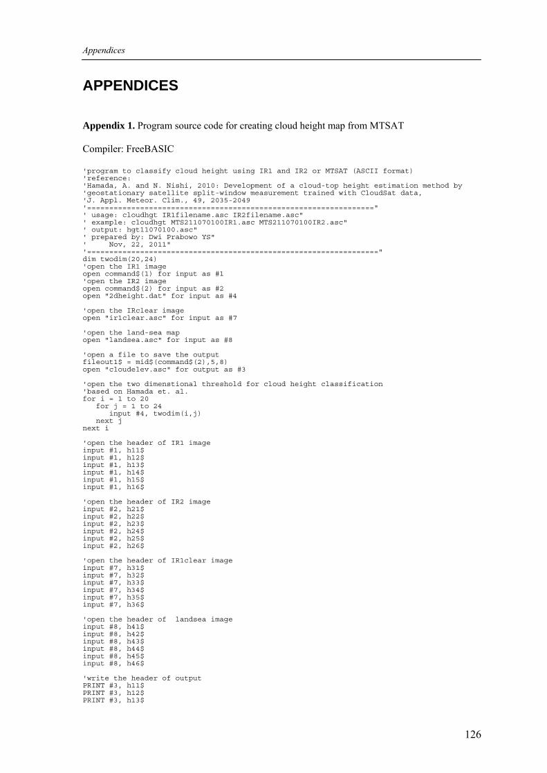
Appendices
126
APPENDICES Appendix 1. Program source code for creating cloud height map from MTSAT Compiler: FreeBASIC 'program to classify cloud height using IR1 and IR2 or MTSAT (ASCII format) 'reference: 'Hamada, A. and N. Nishi, 2010: Development of a cloud-top height estimation method by 'geostationary satellite split-window measurement trained with CloudSat data, 'J. Appl. Meteor. Clim., 49, 2035-2049 '=================================================================" ' usage: cloudhgt IR1filename.asc IR2filename.asc" ' example: cloudhgt MTS211070100IR1.asc MTS211070100IR2.asc" ' output: hgt11070100.asc" ' prepared by: Dwi Prabowo YS" ' Nov, 22, 2011" '==================================================================" dim twodim(20,24) 'open the IR1 image open command$(1) for input as #1 'open the IR2 image open command$(2) for input as #2 open "2dheight.dat" for input as #4 'open the IRclear image open "ir1clear.asc" for input as #7 'open the land-sea map open "landsea.asc" for input as #8 'open a file to save the output fileout1$ = mid$(command$(2),5,8) open "cloudelev.asc" for output as #3 'open the two dimenstional threshold for cloud height classification 'based on Hamada et. al. for i = 1 to 20 for j = 1 to 24 input #4, twodim(i,j) next j next i 'open the header of IR1 image input #1, h11$ input #1, h12$ input #1, h13$ input #1, h14$ input #1, h15$ input #1, h16$ 'open the header of IR2 image input #2, h21$ input #2, h22$ input #2, h23$ input #2, h24$ input #2, h25$ input #2, h26$ 'open the header of IR1clear image input #7, h31$ input #7, h32$ input #7, h33$ input #7, h34$ input #7, h35$ input #7, h36$ 'open the header of landsea image input #8, h41$ input #8, h42$ input #8, h43$ input #8, h44$ input #8, h45$ input #8, h46$ 'write the header of output PRINT #3, h11$ PRINT #3, h12$ PRINT #3, h13$
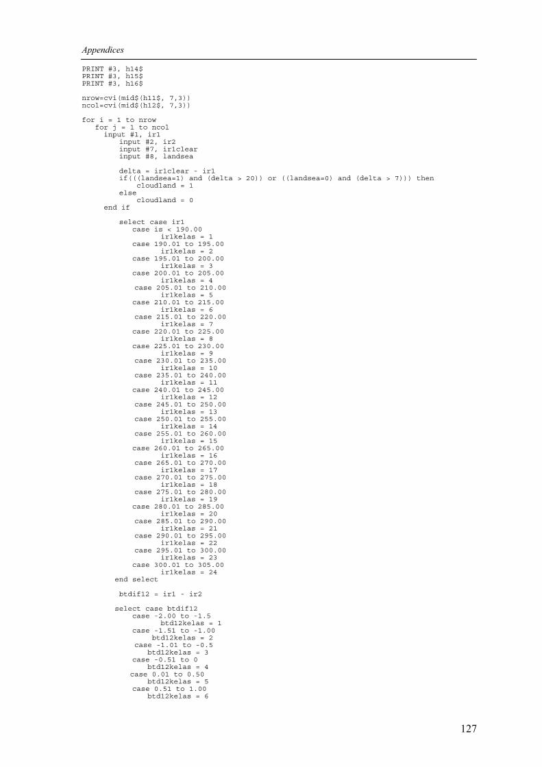
Appendices
127
PRINT #3, h14$ PRINT #3, h15$ PRINT #3, h16$ nrow=cvi(mid$(h11$, 7,3)) ncol=cvi(mid$(h12$, 7,3)) for i = 1 to nrow for j = 1 to ncol input #1, ir1 input #2, ir2 input #7, ir1clear input #8, landsea delta = ir1clear - ir1 if(((landsea=1) and (delta > 20)) or ((landsea=0) and (delta > 7))) then cloudland = 1 else cloudland = 0 end if select case ir1 case is < 190.00 ir1kelas = 1 case 190.01 to 195.00 ir1kelas = 2 case 195.01 to 200.00 ir1kelas = 3 case 200.01 to 205.00 ir1kelas = 4 case 205.01 to 210.00 ir1kelas = 5 case 210.01 to 215.00 ir1kelas = 6 case 215.01 to 220.00 ir1kelas = 7 case 220.01 to 225.00 ir1kelas = 8 case 225.01 to 230.00 ir1kelas = 9 case 230.01 to 235.00 ir1kelas = 10 case 235.01 to 240.00 ir1kelas = 11 case 240.01 to 245.00 ir1kelas = 12 case 245.01 to 250.00 ir1kelas = 13 case 250.01 to 255.00 ir1kelas = 14 case 255.01 to 260.00 ir1kelas = 15 case 260.01 to 265.00 ir1kelas = 16 case 265.01 to 270.00 ir1kelas = 17 case 270.01 to 275.00 ir1kelas = 18 case 275.01 to 280.00 ir1kelas = 19 case 280.01 to 285.00 ir1kelas = 20 case 285.01 to 290.00 ir1kelas = 21 case 290.01 to 295.00 ir1kelas = 22 case 295.01 to 300.00 ir1kelas = 23 case 300.01 to 305.00 ir1kelas = 24 end select btdif12 = ir1 - ir2 select case btdif12 case -2.00 to -1.5 btd12kelas = 1 case -1.51 to -1.00 btd12kelas = 2 case -1.01 to -0.5 btd12kelas = 3 case -0.51 to 0 btd12kelas = 4 case 0.01 to 0.50 btd12kelas = 5 case 0.51 to 1.00 btd12kelas = 6
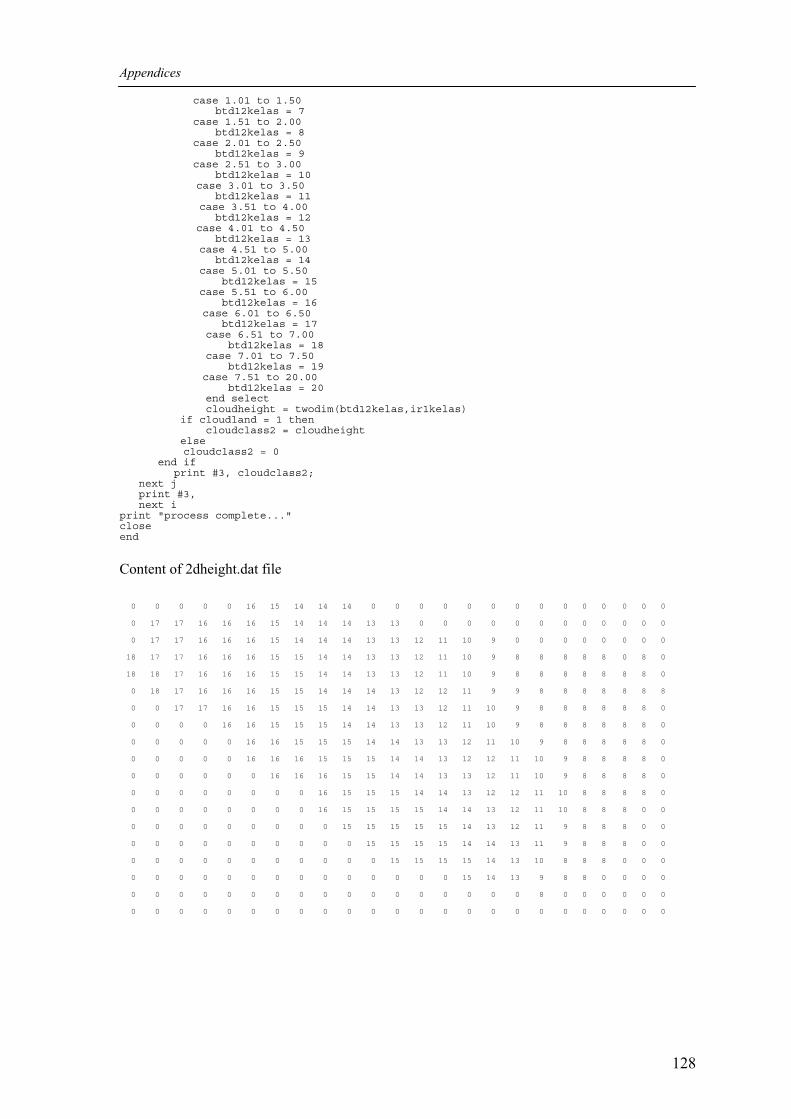
Appendices
128
case 1.01 to 1.50 btd12kelas = 7 case 1.51 to 2.00 btd12kelas = 8 case 2.01 to 2.50 btd12kelas = 9 case 2.51 to 3.00 btd12kelas = 10 case 3.01 to 3.50 btd12kelas = 11 case 3.51 to 4.00 btd12kelas = 12 case 4.01 to 4.50 btd12kelas = 13 case 4.51 to 5.00 btd12kelas = 14 case 5.01 to 5.50 btd12kelas = 15 case 5.51 to 6.00 btd12kelas = 16 case 6.01 to 6.50 btd12kelas = 17 case 6.51 to 7.00 btd12kelas = 18 case 7.01 to 7.50 btd12kelas = 19 case 7.51 to 20.00 btd12kelas = 20 end select cloudheight = twodim(btd12kelas,ir1kelas) if cloudland = 1 then cloudclass2 = cloudheight else cloudclass2 = 0 end if print #3, cloudclass2; next j print #3, next i print "process complete..." close end
Content of 2dheight.dat file
0 0 0 0 0 16 15 14 14 14 0 0 0 0 0 0 0 0 0 0 0 0 0 0
0 17 17 16 16 16 15 14 14 14 13 13 0 0 0 0 0 0 0 0 0 0 0 0
0 17 17 16 16 16 15 14 14 14 13 13 12 11 10 9 0 0 0 0 0 0 0 0
18 17 17 16 16 16 15 15 14 14 13 13 12 11 10 9 8 8 8 8 8 0 8 0
18 18 17 16 16 16 15 15 14 14 13 13 12 11 10 9 8 8 8 8 8 8 8 0
0 18 17 16 16 16 15 15 14 14 14 13 12 12 11 9 9 8 8 8 8 8 8 8
0 0 17 17 16 16 15 15 15 14 14 13 13 12 11 10 9 8 8 8 8 8 8 0
0 0 0 0 16 16 15 15 15 14 14 13 13 12 11 10 9 8 8 8 8 8 8 0
0 0 0 0 0 16 16 15 15 15 14 14 13 13 12 11 10 9 8 8 8 8 8 0
0 0 0 0 0 16 16 16 15 15 15 14 14 13 12 12 11 10 9 8 8 8 8 0
0 0 0 0 0 0 16 16 16 15 15 14 14 13 13 12 11 10 9 8 8 8 8 0
0 0 0 0 0 0 0 0 16 15 15 15 14 14 13 12 12 11 10 8 8 8 8 0
0 0 0 0 0 0 0 0 16 15 15 15 15 14 14 13 12 11 10 8 8 8 0 0
0 0 0 0 0 0 0 0 0 15 15 15 15 15 14 13 12 11 9 8 8 8 0 0
0 0 0 0 0 0 0 0 0 0 15 15 15 15 14 14 13 11 9 8 8 8 0 0
0 0 0 0 0 0 0 0 0 0 0 15 15 15 15 14 13 10 8 8 8 0 0 0
0 0 0 0 0 0 0 0 0 0 0 0 0 0 15 14 13 9 8 8 0 0 0 0
0 0 0 0 0 0 0 0 0 0 0 0 0 0 0 0 0 8 0 0 0 0 0 0
0 0 0 0 0 0 0 0 0 0 0 0 0 0 0 0 0 0 0 0 0 0 0 0
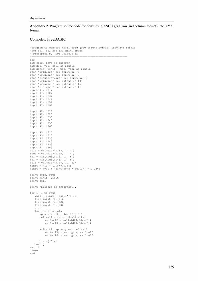
Appendices
129
Appendix 2. Program source code for converting ASCII grid (row and column format) into XYZ format Compiler: FreeBASIC 'program to convert ASCII grid (row column format) into xyz format 'for ir1, ir2 and ir3 MTSAT image ' Prepapred by: Dwi Prabowo YS '============================================================ cls dim cols, rows as integer dim xll, yll, cell as single dim xinit, yinit, xpos, ypos as single open "ir1x.asc" for input as #1 open "ir2x.asc" for input as #2 open "cloudelev.asc" for input as #3 open "ir1x.dat" for output as #4 open "ir2x.dat" for output as #5 open "elev.dat" for output as #6 input #1, h11$ input #1, h12$ input #1, h13$ input #1, h14$ input #1, h15$ input #1, h16$ input #2, h21$ input #2, h22$ input #2, h23$ input #2, h24$ input #2, h25$ input #2, h26$ input #3, h31$ input #3, h32$ input #3, h33$ input #3, h34$ input #3, h35$ input #3, h36$ cols = val(mid$(h11$, 7, 4)) rows = val(mid$(h12$, 7, 4)) xll = val(mid$(h13$, 11, 8)) yll = val(mid$(h14$, 11, 8)) cell = val(mid$(h15$, 10, 6)) xinit = xll + (0.5*0.0334) yinit = (yll + (cint(rows * cell))) - 0.0366 print cols, rows print xinit, yinit print cell print "process is progress..." for i= 1 to rows ypos = yinit - (cell*(i-1)) line input #1, a1$ line input #2, a2$ line input #3, a3$ k = 1 for j = 1 to cols xpos = xinit + (cell*(j-1)) cellval1 = val(mid$(a1$,k,8)) cellval2 = val(mid$(a2$,k,8)) cellval3 = val(mid$(a3$,k,8)) write #4, xpos, ypos, cellval1 write #5, xpos, ypos, cellval2 write #6, xpos, ypos, cellval3 k = (j*8)+1 next j next i close end
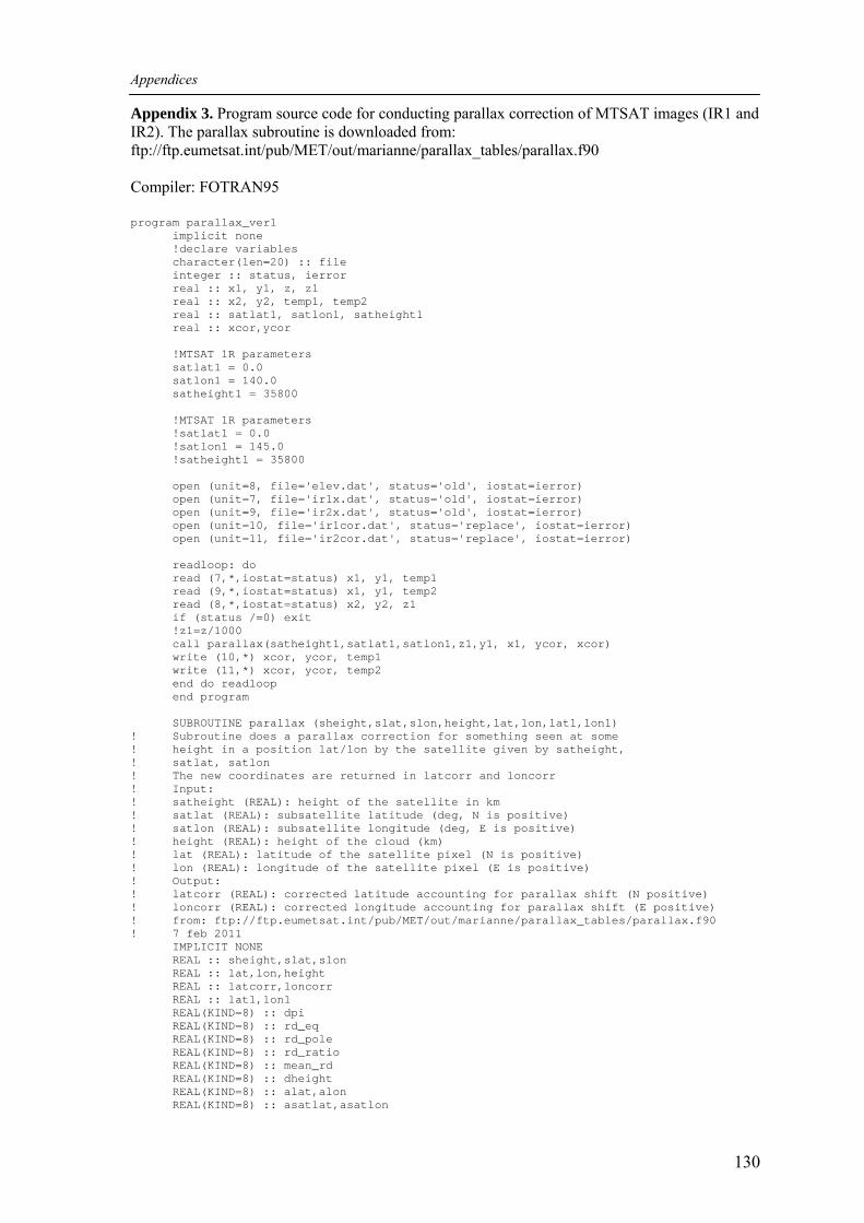
Appendices
130
Appendix 3. Program source code for conducting parallax correction of MTSAT images (IR1 and IR2). The parallax subroutine is downloaded from: ftp://ftp.eumetsat.int/pub/MET/out/marianne/parallax_tables/parallax.f90 Compiler: FOTRAN95 program parallax_ver1 implicit none !declare variables character(len=20) :: file integer :: status, ierror real :: x1, y1, z, z1 real :: x2, y2, temp1, temp2 real :: satlat1, satlon1, satheight1 real :: xcor,ycor !MTSAT 1R parameters satlat1 = 0.0 satlon1 = 140.0 satheight1 = 35800 !MTSAT 1R parameters !satlat1 = 0.0 !satlon1 = 145.0 !satheight1 = 35800 open (unit=8, file='elev.dat', status='old', iostat=ierror) open (unit=7, file='ir1x.dat', status='old', iostat=ierror) open (unit=9, file='ir2x.dat', status='old', iostat=ierror) open (unit=10, file='ir1cor.dat', status='replace', iostat=ierror) open (unit=11, file='ir2cor.dat', status='replace', iostat=ierror) readloop: do read (7,*,iostat=status) x1, y1, temp1 read (9,*,iostat=status) x1, y1, temp2 read (8,*,iostat=status) x2, y2, z1 if (status /=0) exit !z1=z/1000 call parallax(satheight1,satlat1,satlon1,z1,y1, x1, ycor, xcor) write (10,*) xcor, ycor, temp1 write (11,*) xcor, ycor, temp2 end do readloop end program SUBROUTINE parallax (sheight,slat,slon,height,lat,lon,lat1,lon1) ! Subroutine does a parallax correction for something seen at some ! height in a position lat/lon by the satellite given by satheight, ! satlat, satlon ! The new coordinates are returned in latcorr and loncorr ! Input: ! satheight (REAL): height of the satellite in km ! satlat (REAL): subsatellite latitude (deg, N is positive) ! satlon (REAL): subsatellite longitude (deg, E is positive) ! height (REAL): height of the cloud (km) ! lat (REAL): latitude of the satellite pixel (N is positive) ! lon (REAL): longitude of the satellite pixel (E is positive) ! Output: ! latcorr (REAL): corrected latitude accounting for parallax shift (N positive) ! loncorr (REAL): corrected longitude accounting for parallax shift (E positive) ! from: ftp://ftp.eumetsat.int/pub/MET/out/marianne/parallax_tables/parallax.f90 ! 7 feb 2011 IMPLICIT NONE REAL :: sheight,slat,slon REAL :: lat,lon,height REAL :: latcorr,loncorr REAL :: lat1,lon1 REAL(KIND=8) :: dpi REAL(KIND=8) :: rd_eq REAL(KIND=8) :: rd_pole REAL(KIND=8) :: rd_ratio REAL(KIND=8) :: mean_rd REAL(KIND=8) :: dheight REAL(KIND=8) :: alat,alon REAL(KIND=8) :: asatlat,asatlon
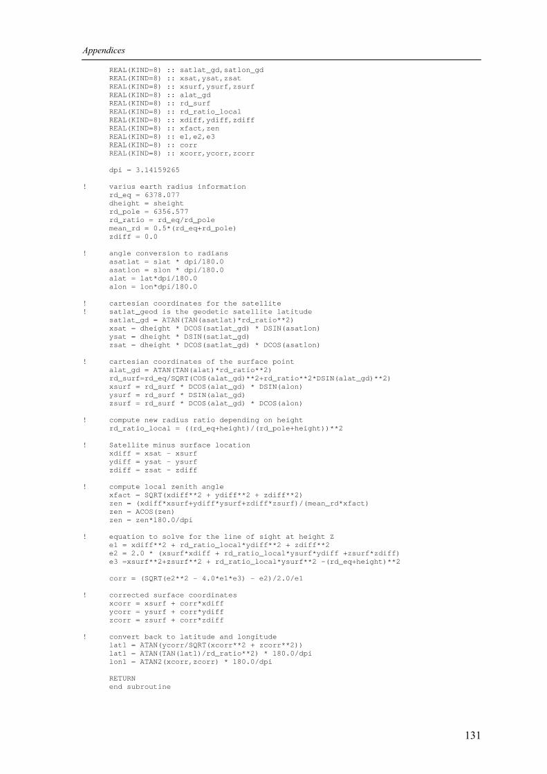
Appendices
131
REAL(KIND=8) :: satlat_gd,satlon_gd REAL(KIND=8) :: xsat,ysat,zsat REAL(KIND=8) :: xsurf,ysurf,zsurf REAL(KIND=8) :: alat_gd REAL(KIND=8) :: rd_surf REAL(KIND=8) :: rd_ratio_local REAL(KIND=8) :: xdiff,ydiff,zdiff REAL(KIND=8) :: xfact,zen REAL(KIND=8) :: e1,e2,e3 REAL(KIND=8) :: corr REAL(KIND=8) :: xcorr,ycorr,zcorr dpi = 3.14159265 ! varius earth radius information rd_eq = 6378.077 dheight = sheight rd_pole = 6356.577 rd_ratio = rd_eq/rd_pole mean_rd = 0.5*(rd_eq+rd_pole) zdiff = 0.0 ! angle conversion to radians asatlat = slat * dpi/180.0 asatlon = slon * dpi/180.0 alat = lat*dpi/180.0 alon = lon*dpi/180.0 ! cartesian coordinates for the satellite ! satlat_geod is the geodetic satellite latitude satlat_gd = ATAN(TAN(asatlat)*rd_ratio**2) xsat = dheight * DCOS(satlat_gd) * DSIN(asatlon) ysat = dheight * DSIN(satlat_gd) zsat = dheight * DCOS(satlat_gd) * DCOS(asatlon) ! cartesian coordinates of the surface point alat_gd = ATAN(TAN(alat)*rd_ratio**2) rd_surf=rd_eq/SQRT(COS(alat_gd)**2+rd_ratio**2*DSIN(alat_gd)**2) xsurf = rd_surf * DCOS(alat_gd) * DSIN(alon) ysurf = rd_surf * DSIN(alat_gd) zsurf = rd_surf * DCOS(alat_gd) * DCOS(alon) ! compute new radius ratio depending on height rd_ratio_local = ((rd_eq+height)/(rd_pole+height))**2 ! Satellite minus surface location xdiff = xsat - xsurf ydiff = ysat - ysurf zdiff = zsat - zdiff ! compute local zenith angle xfact = SQRT(xdiff**2 + ydiff**2 + zdiff**2) zen = (xdiff*xsurf+ydiff*ysurf+zdiff*zsurf)/(mean_rd*xfact) zen = ACOS(zen) zen = zen*180.0/dpi ! equation to solve for the line of sight at height Z e1 = xdiff**2 + rd_ratio_local*ydiff**2 + zdiff**2 e2 = 2.0 * (xsurf*xdiff + rd_ratio_local*ysurf*ydiff +zsurf*zdiff) e3 =xsurf**2+zsurf**2 + rd_ratio_local*ysurf**2 -(rd_eq+height)**2 corr = (SQRT(e2**2 - 4.0*e1*e3) - e2)/2.0/e1 ! corrected surface coordinates xcorr = xsurf + corr*xdiff ycorr = ysurf + corr*ydiff zcorr = zsurf + corr*zdiff ! convert back to latitude and longitude lat1 = ATAN(ycorr/SQRT(xcorr**2 + zcorr**2)) lat1 = ATAN(TAN(lat1)/rd_ratio**2) * 180.0/dpi lon1 = ATAN2(xcorr,zcorr) * 180.0/dpi RETURN end subroutine
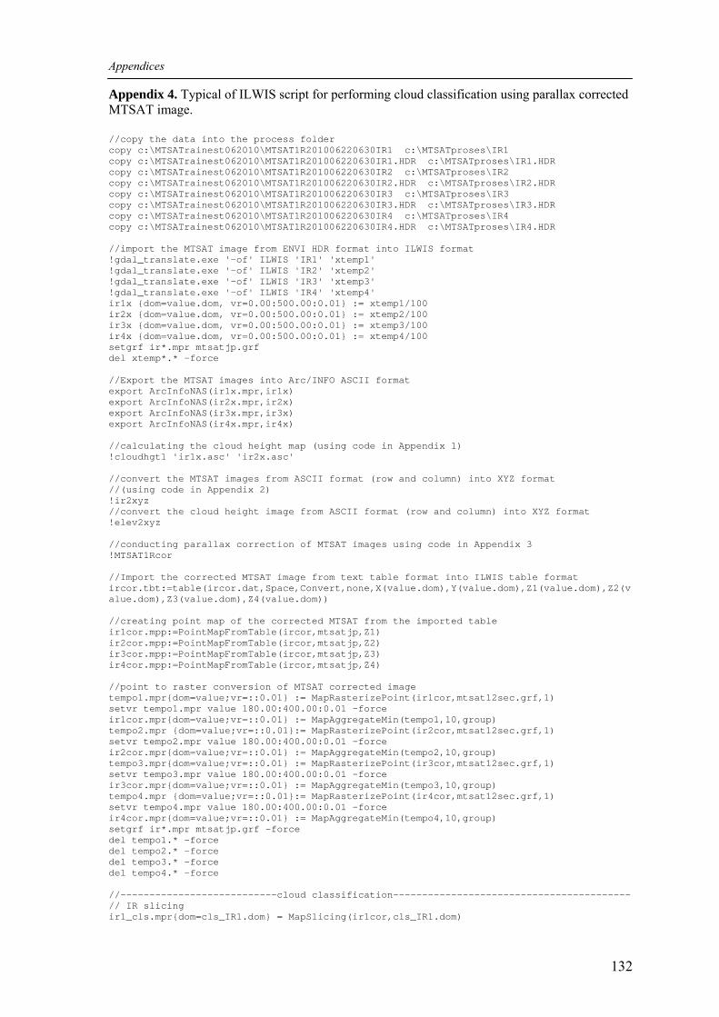
Appendices
132
Appendix 4. Typical of ILWIS script for performing cloud classification using parallax corrected MTSAT image. //copy the data into the process folder copy c:\MTSATrainest062010\MTSAT1R201006220630IR1 c:\MTSATproses\IR1 copy c:\MTSATrainest062010\MTSAT1R201006220630IR1.HDR c:\MTSATproses\IR1.HDR copy c:\MTSATrainest062010\MTSAT1R201006220630IR2 c:\MTSATproses\IR2 copy c:\MTSATrainest062010\MTSAT1R201006220630IR2.HDR c:\MTSATproses\IR2.HDR copy c:\MTSATrainest062010\MTSAT1R201006220630IR3 c:\MTSATproses\IR3 copy c:\MTSATrainest062010\MTSAT1R201006220630IR3.HDR c:\MTSATproses\IR3.HDR copy c:\MTSATrainest062010\MTSAT1R201006220630IR4 c:\MTSATproses\IR4 copy c:\MTSATrainest062010\MTSAT1R201006220630IR4.HDR c:\MTSATproses\IR4.HDR //import the MTSAT image from ENVI HDR format into ILWIS format !gdal_translate.exe '-of' ILWIS 'IR1' 'xtemp1' !gdal_translate.exe '-of' ILWIS 'IR2' 'xtemp2' !gdal_translate.exe '-of' ILWIS 'IR3' 'xtemp3' !gdal_translate.exe '-of' ILWIS 'IR4' 'xtemp4' ir1x {dom=value.dom, vr=0.00:500.00:0.01} := xtemp1/100 ir2x {dom=value.dom, vr=0.00:500.00:0.01} := xtemp2/100 ir3x {dom=value.dom, vr=0.00:500.00:0.01} := xtemp3/100 ir4x {dom=value.dom, vr=0.00:500.00:0.01} := xtemp4/100 setgrf ir*.mpr mtsatjp.grf del xtemp*.* -force //Export the MTSAT images into Arc/INFO ASCII format export ArcInfoNAS(ir1x.mpr,ir1x) export ArcInfoNAS(ir2x.mpr,ir2x) export ArcInfoNAS(ir3x.mpr,ir3x) export ArcInfoNAS(ir4x.mpr,ir4x) //calculating the cloud height map (using code in Appendix 1) !cloudhgt1 'ir1x.asc' 'ir2x.asc' //convert the MTSAT images from ASCII format (row and column) into XYZ format //(using code in Appendix 2) !ir2xyz //convert the cloud height image from ASCII format (row and column) into XYZ format !elev2xyz //conducting parallax correction of MTSAT images using code in Appendix 3 !MTSAT1Rcor //Import the corrected MTSAT image from text table format into ILWIS table format ircor.tbt:=table(ircor.dat,Space,Convert,none,X(value.dom),Y(value.dom),Z1(value.dom),Z2(value.dom),Z3(value.dom),Z4(value.dom)) //creating point map of the corrected MTSAT from the imported table ir1cor.mpp:=PointMapFromTable(ircor,mtsatjp,Z1) ir2cor.mpp:=PointMapFromTable(ircor,mtsatjp,Z2) ir3cor.mpp:=PointMapFromTable(ircor,mtsatjp,Z3) ir4cor.mpp:=PointMapFromTable(ircor,mtsatjp,Z4) //point to raster conversion of MTSAT corrected image tempo1.mpr{dom=value;vr=::0.01} := MapRasterizePoint(ir1cor,mtsat12sec.grf,1) setvr tempo1.mpr value 180.00:400.00:0.01 -force ir1cor.mpr{dom=value;vr=::0.01} := MapAggregateMin(tempo1,10,group) tempo2.mpr {dom=value;vr=::0.01}:= MapRasterizePoint(ir2cor,mtsat12sec.grf,1) setvr tempo2.mpr value 180.00:400.00:0.01 -force ir2cor.mpr{dom=value;vr=::0.01} := MapAggregateMin(tempo2,10,group) tempo3.mpr{dom=value;vr=::0.01} := MapRasterizePoint(ir3cor,mtsat12sec.grf,1) setvr tempo3.mpr value 180.00:400.00:0.01 -force ir3cor.mpr{dom=value;vr=::0.01} := MapAggregateMin(tempo3,10,group) tempo4.mpr {dom=value;vr=::0.01}:= MapRasterizePoint(ir4cor,mtsat12sec.grf,1) setvr tempo4.mpr value 180.00:400.00:0.01 -force ir4cor.mpr{dom=value;vr=::0.01} := MapAggregateMin(tempo4,10,group) setgrf ir*.mpr mtsatjp.grf -force del tempo1.* -force del tempo2.* -force del tempo3.* -force del tempo4.* -force //---------------------------cloud classification----------------------------------------- // IR slicing ir1_cls.mpr{dom=cls_IR1.dom} = MapSlicing(ir1cor,cls_IR1.dom)
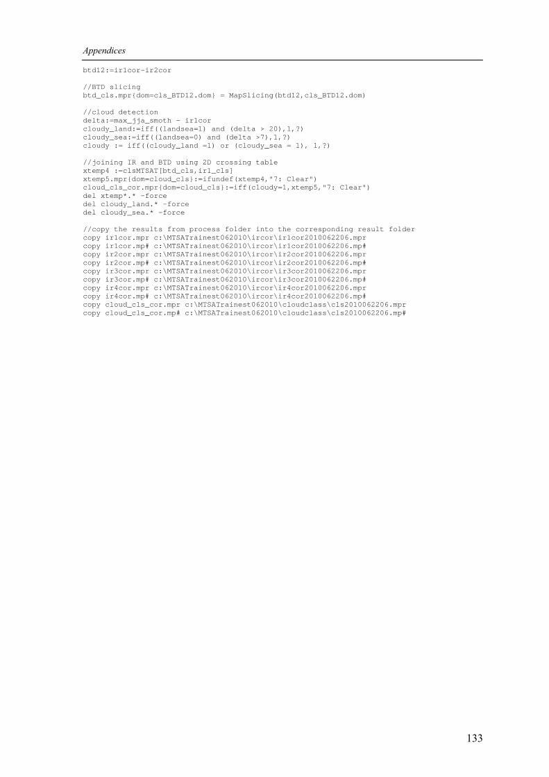
Appendices
133
btd12:=ir1cor-ir2cor //BTD slicing btd_cls.mpr{dom=cls_BTD12.dom} = MapSlicing(btd12,cls_BTD12.dom) //cloud detection delta:=max_jja_smoth - ir1cor cloudy_land:=iff((landsea=1) and (delta > 20),1,?) cloudy_sea:=iff((landsea=0) and (delta >7),1,?) cloudy := iff((cloudy_land =1) or (cloudy_sea = 1), 1,?) //joining IR and BTD using 2D crossing table xtemp4 :=clsMTSAT[btd_cls,ir1_cls] xtemp5.mpr{dom=cloud_cls}:=ifundef(xtemp4,"7: Clear") cloud_cls_cor.mpr{dom=cloud_cls}:=iff(cloudy=1,xtemp5,"7: Clear") del xtemp*.* -force del cloudy_land.* -force del cloudy_sea.* -force //copy the results from process folder into the corresponding result folder copy ir1cor.mpr c:\MTSATrainest062010\ircor\ir1cor2010062206.mpr copy ir1cor.mp# c:\MTSATrainest062010\ircor\ir1cor2010062206.mp# copy ir2cor.mpr c:\MTSATrainest062010\ircor\ir2cor2010062206.mpr copy ir2cor.mp# c:\MTSATrainest062010\ircor\ir2cor2010062206.mp# copy ir3cor.mpr c:\MTSATrainest062010\ircor\ir3cor2010062206.mpr copy ir3cor.mp# c:\MTSATrainest062010\ircor\ir3cor2010062206.mp# copy ir4cor.mpr c:\MTSATrainest062010\ircor\ir4cor2010062206.mpr copy ir4cor.mp# c:\MTSATrainest062010\ircor\ir4cor2010062206.mp# copy cloud_cls_cor.mpr c:\MTSATrainest062010\cloudclass\cls2010062206.mpr copy cloud_cls_cor.mp# c:\MTSATrainest062010\cloudclass\cls2010062206.mp#
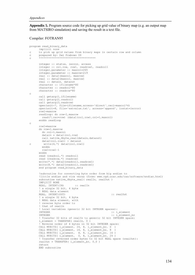
Appendices
134
Appendix 5. Program source code for picking up grid value of binary map (e.g. an output map from MATSIRO simulation) and saving the result in a text file. Compiler: FOTRAN95 program read_binary_data implicit none c to pick up grid values from binary maps in certain row and column c prepared by: Dwi Prabowo YS c ************************************ integer :: status, ierror, access integer :: col,row, row1, readrow1, readcol1 integer,parameter :: maxcol=265 integer,parameter :: maxrow=219 real :: data1(maxcol, maxrow) real :: data2(maxcol, maxrow) real :: datain, dataout character :: ifilename*80 character :: readcol*80 character :: readrow*80 c call getarg(1,ifilename) call getarg(2,readcol) call getarg(3,readrow) open(unit=7, file=ifilename,access='direct',recl=maxcol*4) open(unit=8, file='extvalue.txt', access='append', iostat=ierror) row1=maxrow readloop: do row=1,maxrow read(7,rec=row) (data1(col,row),col=1,maxcol) enddo readloop c row1=maxrow do row=1,maxrow do col=1,maxcol datain = data1(col,row) call native_4byte_real(datain,dataout) data2(col,row1) = dataout c write(6,*) data2(col,row1) enddo row1=row1-1 enddo read (readcol,*) readcol1 read (readrow,*) readrow1 write(*,*) data2(readcol1,readrow1) write(8,*) data2(readcol1,readrow1) end program read_binary_data !subroutine for converting byte order from big endian to !little endian and vice versa (from: www.cgd.ucar.edu/cas/software/endian.html) subroutine native_4byte_real( realIn, realOut ) IMPLICIT NONE REAL, INTENT(IN) :: realIn ! a single 32 bit, 4 byte ! REAL data element REAL, INTENT(OUT) :: realOut ! a single 32 bit, 4 byte ! REAL data element, with ! reverse byte order to ! that of realIn ! Local variables (generic 32 bit INTEGER spaces): INTEGER :: i_element INTEGER :: i_element_br ! Transfer 32 bits of realIn to generic 32 bit INTEGER space: i_element = TRANSFER( realIn, 0 ) ! Reverse order of 4 bytes in 32 bit INTEGER space: CALL MVBITS( i_element, 24, 8, i_element_br, 0 ) CALL MVBITS( i_element, 16, 8, i_element_br, 8 ) CALL MVBITS( i_element, 8, 8, i_element_br, 16 ) CALL MVBITS( i_element, 0, 8, i_element_br, 24 ) ! Transfer reversed order bytes to 32 bit REAL space (realOut): realOut = TRANSFER( i_element_br, 0.0 ) return END subroutine
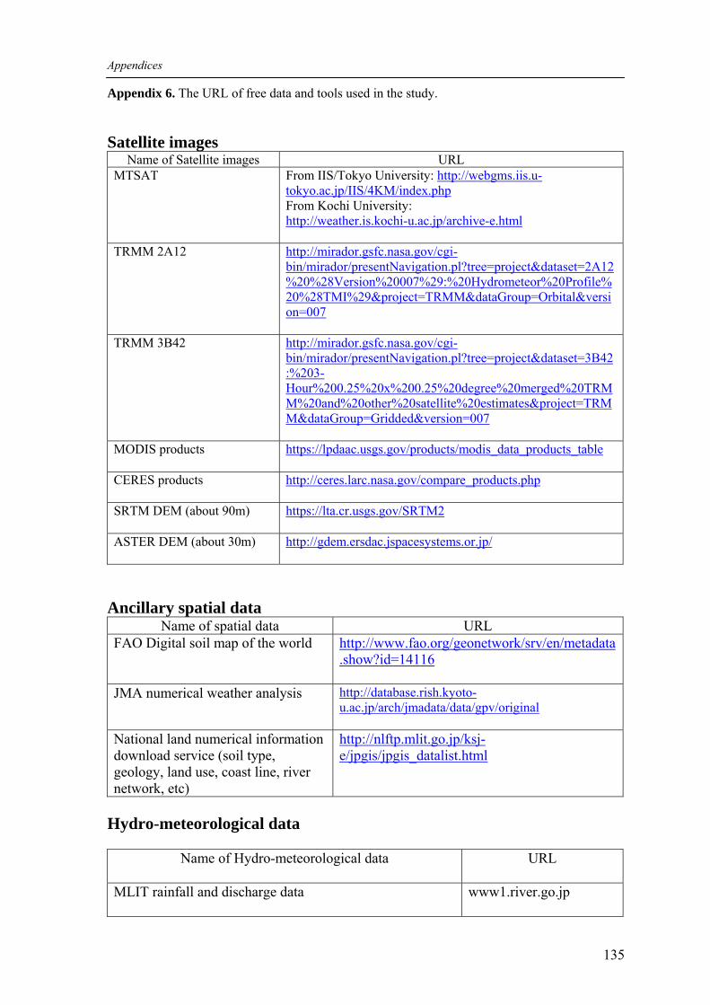
Appendices
135
Appendix 6. The URL of free data and tools used in the study. Satellite images
Name of Satellite images URL MTSAT From IIS/Tokyo University: http://webgms.iis.u-
tokyo.ac.jp/IIS/4KM/index.php From Kochi University: http://weather.is.kochi-u.ac.jp/archive-e.html
TRMM 2A12 http://mirador.gsfc.nasa.gov/cgi-bin/mirador/presentNavigation.pl?tree=project&dataset=2A12%20%28Version%20007%29:%20Hydrometeor%20Profile%20%28TMI%29&project=TRMM&dataGroup=Orbital&version=007
TRMM 3B42 http://mirador.gsfc.nasa.gov/cgi-bin/mirador/presentNavigation.pl?tree=project&dataset=3B42:%203-Hour%200.25%20x%200.25%20degree%20merged%20TRMM%20and%20other%20satellite%20estimates&project=TRMM&dataGroup=Gridded&version=007
MODIS products https://lpdaac.usgs.gov/products/modis_data_products_table
CERES products http://ceres.larc.nasa.gov/compare_products.php
SRTM DEM (about 90m) https://lta.cr.usgs.gov/SRTM2
ASTER DEM (about 30m) http://gdem.ersdac.jspacesystems.or.jp/
Ancillary spatial data
Name of spatial data URL FAO Digital soil map of the world http://www.fao.org/geonetwork/srv/en/metadata
.show?id=14116
JMA numerical weather analysis http://database.rish.kyoto-u.ac.jp/arch/jmadata/data/gpv/original
National land numerical information download service (soil type, geology, land use, coast line, river network, etc)
http://nlftp.mlit.go.jp/ksj-e/jpgis/jpgis_datalist.html
Hydro-meteorological data
Name of Hydro-meteorological data
URL
MLIT rainfall and discharge data www1.river.go.jp
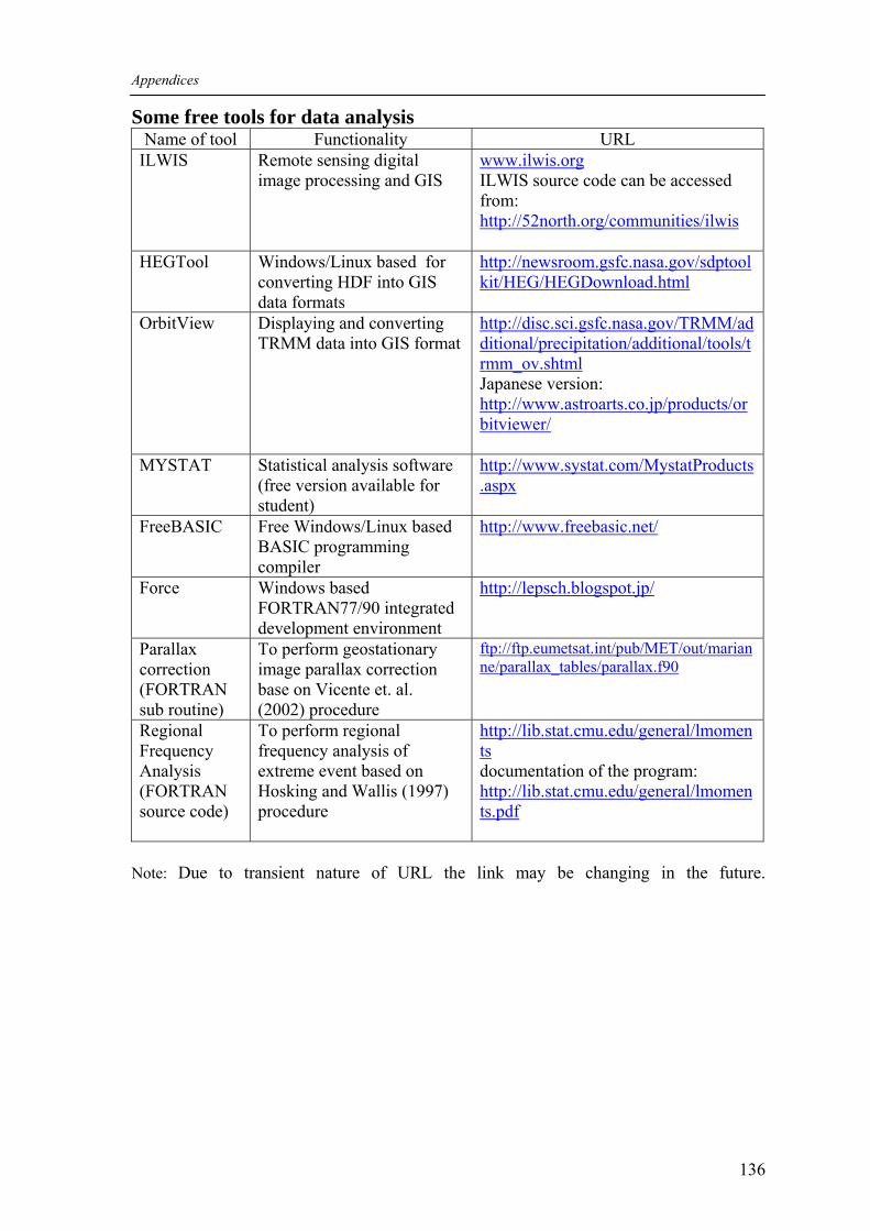
Appendices
136
Some free tools for data analysis Name of tool Functionality URL
ILWIS Remote sensing digital image processing and GIS
www.ilwis.org ILWIS source code can be accessed from: http://52north.org/communities/ilwis
HEGTool Windows/Linux based for converting HDF into GIS data formats
http://newsroom.gsfc.nasa.gov/sdptoolkit/HEG/HEGDownload.html
OrbitView Displaying and converting TRMM data into GIS format
http://disc.sci.gsfc.nasa.gov/TRMM/additional/precipitation/additional/tools/trmm_ov.shtml Japanese version: http://www.astroarts.co.jp/products/orbitviewer/
MYSTAT Statistical analysis software (free version available for student)
http://www.systat.com/MystatProducts.aspx
FreeBASIC Free Windows/Linux based BASIC programming compiler
http://www.freebasic.net/
Force Windows based FORTRAN77/90 integrated development environment
http://lepsch.blogspot.jp/
Parallax correction (FORTRAN sub routine)
To perform geostationary image parallax correction base on Vicente et. al. (2002) procedure
ftp://ftp.eumetsat.int/pub/MET/out/marianne/parallax_tables/parallax.f90
Regional Frequency Analysis (FORTRAN source code)
To perform regional frequency analysis of extreme event based on Hosking and Wallis (1997) procedure
http://lib.stat.cmu.edu/general/lmoments documentation of the program: http://lib.stat.cmu.edu/general/lmoments.pdf
Note: Due to transient nature of URL the link may be changing in the future.

137
CURRICULUM VITAE Home address: Indonesia Current address: Hokkaido University International House Kita 8, Kita 8, Nishi 11, 1-4-101, Sapporo Name: Dwi Prabowo Yuga Suseno Date of birth: 04/11/1975 Educational background 01/07/1993 Senior High School, Kebumen, Central Java, Indonesia (graduated). 01/08/1993 Department of Cartography and Remote Sensing, Faculty of Geography, Gadjah
Mada University, Yogyakarta, Indonesia (enrolled). 31/08/1998 -same as above- (graduated). 01/08/2007 Master’s Program (double degree), Geoinformation for Spatial Planning and Risk
Management, Gadjah Mada University, Yogyakarta, Indonesia and International Institute for Geoinformation Science and Earth Observation (ITC), Enschede, The Netherlands (enrolled).
29/04/2009 -same as above- (graduated). 01/10/2010 Doctoral Program, Division of Field Engineering for Environment, Graduate
School of Engineering, Hokkaido University (enrolled). 25/09/2013 -same as above- (graduated). Professional background 01/09/1998 Forest Fire Prevention Management Project, Japan International Corporation
Agency (JICA), Bogor, Indonesia (joined). 01/09/1998 Early Warning System Expert Assistant, same as above (assigned). 31/08/1999 –same as above– (resigned). 01/09/1999 Forest Watch Indonesia, Bogor, Indonesia (joined). 01/09/1999 Remote Sensing and Geographic Information System (GIS) specialist, same as
above (assigned). 26/12/2001 –same as above– (resigned). 27/12/2001 Watershed management office of Indragiri-Rokan, Ministry of Forestry Republic
of Indonesia, Pekanbaru, Riau, Indonesia (joined). 27/12/2001 Government officer staff (assigned until now). Research background 01/08/2007~ 29/04/2009
Geoinformation for Spatial Planning and Risk Management,Gadjah Mada University, Yogyakarta, Indonesia and International Institute for Geoinformation Science and Earth Observation (ITC),”Geostationary satellite based rainfall estimation for hazard studies and validation, A case study of Java Island, Indonesia” involved in during Master’s program.
01/10/2010~ present Division of Field Engineering for Environment, Graduate School of Engineering, Hokkaido University, ” The use geostationary satellite based rainfall estimation and rainfall-runoff modelling for regional flash flood assessment” involved in during Doctoral program.
Prize
I certify that the above are true records. Date: 19/6/2013 (Dwi Prabowo Yuga Suseno)
138
LIST OF PUBLICATIONS Dissertation submitted for the degree
I. Title: The use geostationary satellite based rainfall estimation and rainfall-runoff modelling for regional flash flood assessment.
Peer reviewed papers:
1. Suseno, Dwi Prabowo Yuga, T. J. Yamada, 2011, Geostationary Satellite Based Rainfall Estimation and Validation: A Case Study of Java Island, Indonesia, Journal of Japan Society of Civil Engineers, Ser. B1 (Hydraulic Engineering), Volume 67, Issue 4, pp. I_43-I_48
2. Suseno, Dwi Prabowo Yuga, T. J. Yamada, 2011, The Use of Cloud Type Classification To Improve Geostationary Based Rainfall Estimation. 9th International Symposium on Southeast Asian Water Environment, Dec 1st - 3rd 2011 Bangkok City, Thailand.
3. Suseno, Dwi Prabowo Yuga, T. J. Yamada, 2012, The use of geostationary based rainfall estimation for characterizing strom severity, Journal of Japan Society of Civil Engineers, Ser. B1 (Hydraulic Engineering), Volume 68, Issue 4, pp. I_175-I_180
4. Suseno, Dwi Prabowo Yuga, T. J. Yamada, 2012, Two-dimensional threshold-based cloud-type classification using MTSAT data, Remote Sensing Letters, Vol. 3, No. 8, pp. 737 - 746
5. Suseno, Dwi Prabowo Yuga, T. J. Yamada, 2013, The role of GPS precipitable water vapor and atmospheric stability index on the statistically-based rainfall estimation using MTSAT data, Submitted to Journal of Hydrometeorology (accepted).
Oral presentation on conference:
1. Suseno, Dwi Prabowo Yuga, T. J. Yamada, 2011,Geostationary satellite based rainfall estimation and validation and its future development, The 67th Japan Society of Civil Engineers Local Conference, Feb 2011, Tomakomai, Japan.
2. Suseno, Dwi Prabowo Yuga, T. J. Yamada, 2011, Characterizing storm severity by using geostationary satellite rainfall, Proceedings of 2011 Annual conference, Japan Society of Hydrology and Water Resources, Aug 30th - Sep 1st , 2011, Kyoto, Japan
3. Suseno, Dwi Prabowo Yuga, T. J. Yamada, 2013, The Use of MTSAT and atmospheric environmental condition datasets for storm rainfall estimation. The 1st International Doctoral Symposium in Structural and Hydraulic Engineering, Feb 7th -9th 2013, Sapporo, Japan.
Poster Presentation:
1. Suseno, Dwi Prabowo Yuga, T. J. Yamada, 2011, The Use of Cloud Type Classification To Improve Geostationary Satellite Based Rainfall Estimation, Japan Geoscience Union Meeting 2011, Tokyo, Japan.
2. Suseno, Dwi Prabowo Yuga, T. J. Yamada, 2012, Flash flood severity assessment using Hydro-morpho-climatic approach, Hokkaido University and Chungbuk National University Joint Symposium, Sapporo, Japan.
Co-author for peer reviewed papers:
1. Wada, Takuya, T. J. Yamada, Dwi Prabowo Yuga Suseno, 2012, Formation and environment of a line-shaped rainfall system observed in Niigata-Fukushima Heavy Rainfall in July 2011 (in Japanese), Journal of Japan Society of Civil Engineers, Ser. B1 (Hydraulic Engineering), Volume 68, Issue 4, pp. I_397-I_402
2. Yamato, Watanabe, T. J. Yamada, Dwi Prabowo Yuga Suseno, 2013, The Cloud Climatology Over Southeastern Asian Regions By Using MTSAT Cloud Classification (in Japanese), Journal of Japan Society of Civil Engineers, Ser. B1 (Hydraulic Engineering), Volume 69, Issue 4, pp. I_301-I_306