Theory in Materials ScienceTheory in Materials Science

44rdrd lecturelectureApplications of the first principles calculationApplications of the first principles calculation

for the high pressure physicsfor the high pressure physics

Professor Naoshi Suzuki & Associate Professor Koichi Kusakabe

Graduate School of Engineering Science, Osaka University

ab initio calculations

• Simulations utilizing experimental values and/or empirical inter-atomic potentials.

1. There is limitation in applicable pheno-mena and the methods have less predictability.

2. The methods require less computation time and may deal with large systems.

• Simulations starting from the first principles without empirical information. (ab initiomethods)

1. The methods are widely applicabile and possess potential to predict new phenomena and novel materials.

2. The methods may cost huge computation time.

New trends in computational material science

• Progress in Computational Techniques– Numerical integration of differential equations for

complex multi-dimensional systems became possible.(new solvers, new optimization techniques, etc.)

– Progress in high-performance computers is available.(paralleled machines, CPU with high clock speed, etc.)

Simulations reproducing real experimentswere realized.

Innovation in Material Science! Materials design!

High-Pressure Physics and Computational Material Science

• Difficulty in real experiments• In-situ observation in atomic scaleunder high pressure

• Ultra-high pressure unreachable byconventional techniques

These requirements are partly solved in real experiments.However,

Computational approaches give an alternative solution.

The first-principles electronic-statecalculation under high pressure

Classical molecular dynamicsClassical molecular dynamics First-principles electronicstate calculations

First-principles electronicstate calculations

• Empirical potentials• Simulation at a constant temperature• Simulation at a constant pressure

Volume and temperature are variable.⇒ Structural transformation

• Density functional theory + LDA or GGA• Car-Parinello method, CG• Planewave expansion + FFT• Pseudo-potential method

High-speed calculation of electronic states, inter-atomic forces and internal stress

Unify

First-principles molecular dynamicsunder constant pressure & temperatureFirst-principles molecular dynamics

under constant pressure & temperature

Simulation of unknown structures and novel materials!

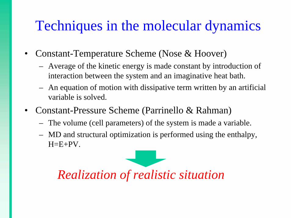
Techniques in the molecular dynamics

• Constant-Temperature Scheme (Nose & Hoover)– Average of the kinetic energy is made constant by introduction of

interaction between the system and an imaginative heat bath.– An equation of motion with dissipative term written by an artificial

variable is solved.

• Constant-Pressure Scheme (Parrinello & Rahman)– The volume (cell parameters) of the system is made a variable.– MD and structural optimization is performed using the enthalpy,

H=E+PV.

Realization of realistic situation

The density functional theory– Hohenberg-Kohn's theorem & Kohn-Sham theory– Levy's DFT (Density Functional theory)

The energy of the ground state is given by the minimum of anEnergy functional of the single-particle density.

EGS = d 3r vext(r) nGS(r) + F[nGS]

F[n] = min

Φ → n (r) Φ|T + Vee|Φ

The Kohn-Sham equation: – h2

2m∇2 + vext(r) + e2 d 3r' n(r)|r – r'| + δExc[n]

δn(r) φi = εiφi

This equation is solvable by computation with a high speed bythe Car-Parrinello method or CG.

Characteristics of basis sets for DFT calculation

• Plane-wave expansion method with pseudo-potentials• Since plane waves are independent of position of atoms, the result is

accurate.• Accuracy of the calculation is determined by the maximum energy of plane

waves.• The kinetic energy is diagonal in the Fourier space, while the potential

energy is diagonal in the real space. Thus FFT is used.• The Hellmann-Feynman force and the quantum stress are easily obtained.

• FLAPW (Full-potential linearlized augmented plane wave)• The wave functions are expanded in spherical waves in an atomic sphere

and in plane waves out of the sphere.• Accuracy is determined by number of partial waves and the maximum

energy of plane waves.• Less ambiguity compared to the pseudo-potential method.• Pulay force has to be evaluated.

The local density approximation I.

The local density approximation II.

The local density approximation III.

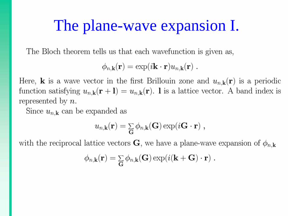
The plane-wave expansion I.

The plane-wave expansion II.

• Dimension of the matrix can be O(103) or O(104).• The diagonalization is often performed using the Housholder method of the conjugate gradient method (CG).

However, • the process to find the ground state is regarded as an optimization process forthe energy functional in the function space.

The Car-Parrinello method (Conceptually different idea)

The pseudopotential I.

Ca 4s orbital

Ca 4p orbitalAll electron calc.Pseudization calc.

All electron calc.Pseudization calc.

The pseudopotential II.

The pseudopotential III.

The Hellmann-Feynman force

The calculation scheme of FPMD at a constant pressure

Input:AtomsUnit Cell

External Pressure

{RI}{a0}

{Ψi}

{F}{σ}

{ε}

a = (1 +ε ) a0

Pext

Wave Functions

HF ForceQuantum Stress

Molecular Dynamics

{RI}

Convergence check

update

using {F} {σ}

{ε}{RI} update

a = (1 + ε)a0

by CG method

Optimized {Ψ i} {ε}{RI}

Kohn-Sham eq.{

Structuraloptimization

Moleculardynamics

What is expected for FPMD?

• Accuracy– If the electronic state is well described, accurate within

the Born-Oppenheimer approximation.– See examples below.

• Power– Structural transformation is reproducible for any kind of

materials in principle.– Limited by computational resources and by accuracy of

DFT-LDA (DFT-GGA).

We can show some examples onthe prediction of new materials.

Graphite under high pressure

• Purpose– We show accuracy of FPMD by comparing real

experiments and our calculations• Examples1.Graphite-diamond transformation2.Graphite ball under high pressure

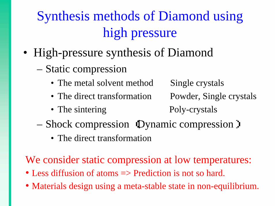
Synthesis methods of Diamond using high pressure

• High-pressure synthesis of Diamond– Static compression

• The metal solvent method Single crystals• The direct transformation Powder, Single crystals• The sintering Poly-crystals

– Shock compression （Dynamic compression）• The direct transformation

We consider static compression at low temperatures:• Less diffusion of atoms => Prediction is not so hard.• Materials design using a meta-stable state in non-equilibrium.

Graphite-Diamond transformation at high-pressure

Graphite(AB stacking)

Hexagonal Diamond(AB stacking)

Cubic Diamond(ABC stacking)

a

b

c

Compression Compression

Monoclinic

[001]

[111]

Kish graphite

Pc = 14 ~ 18 GPa ( Static )Room temperatureT. Yagi et al. ('92)

Hexagonal DiamondPolycrystalline graphite

Pc = 14 ~ 20 GPa ( Static )Room temperatureS. Endo et al. ('94)

Force inversion technique to search for the saddle point

P1

L1

L2

P2

by Tsuneyuki et al.

1) Determine a direction between L1 and L2 in multi-dimensional phase space.2) Obtain a projection of the inter-atomic force (the blue arrow) on the direction from L1 to L2.3) Make inversion of the projection in 2) and obtain an artificial force (the black arrow).4) Optimization with the force in 3) gives the saddle point.

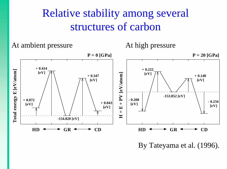
Relative stability among several structures of carbon

At ambient pressure At high pressure

.Tota

l ene

rgy

E [e

V/a

tom

]

HD GR CD

P = 0 [GPa]

+ 0.043[eV]

+ 0.072[eV]

+ 0.414[eV]

+ 0.347[eV]

-154.820 [eV] H =

E +

PV

[eV

/ato

m]

HD GR CD

P = 20 [GPa]

- 0.208[eV]

+ 0.222[eV] + 0.148

[eV]

- 0.234[eV]

-153.852 [eV]

By Tateyama et al. (1996).

Graphite-diamond transformation in a FPMD simulation

At ambient pressure At high pressure

Formation of new bondings at the transformation

• White objects are carbonatoms and yellow iso-surfaces represent chargedensity of electrons.

• We see new bondingrepresented by bondingcharge between graphitelayers.

• Sliding of layersoccurs due to formationof sp3 bond connections.

Simulation

Electronic band structure of graphite under high pressure

43 GPa0 GPa

The system is a semimetal. The system is a metal.

Electronic wavefunction in graphite

• a π state at the Γ point in the π band.

• It is extending in the whole lattice structure.

π orbitalCarbon atom