Embed Size (px)
Citation preview
Thermal optimization of VEO+ projector
Trying to reduce noise of the Veo+ projector by DOE (Design of Experiment) tests to find an
optimal solution for the fan algorithm while considering the thermal specifics of the unit
CEM HIZLI
Mälardalen University IDE
Optea AB
20.07.2010
Master’s Thesis at Mälardalen University, July 2010
Supervisor and Examiner: Lars Asplund
Supervisor at Optea AB: Esteban Arboix
1
Abstract
The Veo+ projector is using a cooling system that consists of fan and blowers. This system is
cooling the electronic components of the device and the lamp of the projector, however
extracting a high noise. To lower this noise the rpm speeds (rotational speed) of the fan and
blowers should be decreased. Thus, lowering the speed will result in higher temperature
values in whole system (inside the device). While lowering the speed, the higher temperature
values should be kept within the thermal design specifications of the electronic components.
The purpose of this thesis work is to find an optimal solution with lower rpm speeds of the
fan and blowers while keeping the temperatures of the various components of the device
(touch temperature of the enclosure and electronic components) within the temperature
design limits. Before testing the device to find the optimum state, the design limits of the
device are determined. Then, by using the design of experiment methods like Taguchi, the
optimum state for the device within the design specifications is obtained. Finally, additional
tests are applied within the optimum state to demonstrate a fan algorithm as a final solution.
While doing the experiments thermocouples are used for measuring the component
temperatures.
Keywords: Projector, thermal optimization, thermocouple, design of experiments, taguchi,
fan, blower.

2
Acknowledgement
In this part, I would like to add two important changes how the thesis work changed and
challenged how I see the world. In additional, at final part I want to acknowledge the people
who helped me in this challenging journey.
First, when I think about the time before the thesis work I see a big difference on my problem
solving skills. I could say this development is achieved by learning to take more
responsibility in decision making process and always trying to plan one step ahead.
Secondly, in the last few months while doing the thesis work I realized that; there is always
room for developing new ideas and adding more contributions to any work. To drive this
continuous contribution I could enlist two features as desire and hard work. In this
experience, I learned that those two key features are helping human beings to solve the new
challenges throughout their life.
Finally, I should acknowledge the contributions of my supervisors Esteban Arboix and Lars
Asplund as with their valuable feedback on my work and their guidance during the process.
I also would like to thank Yijun Zhao for our discussions related to the project.
July 2010
CEM HIZLI
3
Contents
1 Introduction…………………………………………………………………………….4
1.1 Background…………………………………………………………………………………...…….....4
1.2 General Description of the Thesis work……………………………………………………….…….4
1.3 Detailed Description of the Thesis work….……….…………………………………………………5
1.4 Structure of the Report……….……….………………………………………………………...……7
2 Detailed Status Check............……………….……………….…………………….…...8
2.1 Before the detailed status check...………………...….……………….……………………………….8
2.2 During the detailed status check…...…….………….…………………….……………………….….8
2.3 After the detailed status check………………………….………………….………………………….9
2.4 Equipments that are used….……………………………………………………….…………….......12
2.5 Short List of the tools …………………………………………………………………………….......19
2.6 Test Setup………………………………………………………………………………………….......19
2.7 Summary………………………………………………………………………………………………21
3 Experiments…………………………………………………………………………….21
3.1 Introduction ………………………………………………………………………………………..…21
3.2 Taguchi method……………………………………………………………………………………….22
3.3 Implementing Taguchi method for project………………………………………………………….23
3.4 Experimental Runs……………………………………………………………………………………26
3.5 Summary ………………..………………………………………………………………………....….34
4 Further Experiments………………………………………………….………....….....34
4.1 Introduction……………………………………………………………………………………….......34
4.2 Status check and absolute test………….……………………………………………….…………....35
4.3 Selection of levels……………………………………………………………………………………...35
4.4 Summary………………………………………………………………………………………………36
5 Fan Algorithm………………………………………………………………………….37
5.1 Introduction…………………………………………………………………………………………...37
5.2 Fan algorithm illustration……………………………………….……………………………………38
5.3 Discussion on algorithm illustration………………………………………………….……………...39
5.4 Summary………………………………………………………………………………………………39
6 Conclusion and recommendations…………………………………………………….39
6.1 Conclusion……………………………………………………………………………………………..39
6.2 Recommendations for future design……………………………………………………………..…..40
References……………………………………………………………………………...……41
Appendix…………………………………………………………………………………….42

4
1 Introduction
1.1 Background
Optea AB, a start-up company based in Teknikhöjden; Stockholm, has developed a world
class innovative projector (Veo+) to be sold in new types of markets, such as marine, car and
caravan market. The company is also working on other innovative projection systems such
as Head's Up Display applications for construction vehicles.
Figure 1: Veo+ projector.
Veo+ projector is based on 12V Digital Light Processing (DLP) technology and using a
Philips Ujoy lamp as a lighting source. The projector is quiet portable with its small
dimensions and light weight. Market introduction of the projector is expected in 2010. [1]
1.2 General Description of the Thesis Work
General description of the work done could be summarized in five parts as listed below:
• Determining and updating the thermal design specifications of the Veo+ projector.
• Detailed thermal status check of the device before the design of experiments.
• Thermal optimization to reduce noise of the Veo+ unit by using design of
experiments.
• Suggesting a solution for the fan algorithm considering the data of temperature sensor
within the device.
• Giving recommendations for the future designs.
The work at the Optea AB is done under guidance of a mechanical engineer (Esteban Arboix)
and with the collaboration of electronic engineer (Yijun Zhao) between February 2010 and
July 2010 on daily basis.

5
1.3 Detailed Description of the Thesis work
For demonstrating the projector, we could think the projector as a rectangle and divide this
rectangle into two parts. These two parts are main module and lamp module. The main
module has most of the electronic parts and lamp module has the light source and the cooling
units.
Figure 2: Veo+ unit general airflows.
The Figure 2 is showing how cooling system of Optea Veo+ works in the design. The yellow
circle is representing the lamp of the projector and it is heating the design. The red rectangles
are fan and blowers of the system to create air flow (showed by the arrows) for decreasing the
heat at the projector. The green dot is the temperature sensors to give a feedback about the
temperature.
The main goal of this thesis work is to find an optimal state for the fan and blowers (finding
optimal speeds). This optimal state will help device to adjust the inner temperature values
with reference to the temperature requirements of the device in an environment (using the
green temperature sensor). Lowering the speeds of fan and blowers, is helping to decrease
the noise of the device, however it is causing the temperature values to increase. Thus, while
lowering the speeds of fan and blowers, the temperature design requirements should not be
exceeded. Those design requirements are including all the important electronic components,
the aluminum enclosure and the air flow units (fan and blowers). In additional, the ambient
pressure and the temperature that the device is operating are the important challenges to
experiment the device for finding an optimum recommendation.

6
During the first stage of the thesis work, the suitable thermocouples, adhesives (for attaching
the thermocouples), data loggers (for collecting the data) and stroboscopes (for finding rpm
speeds of fan and blowers) are searched in the market. Then for its common usage and
suitable price, K type thermocouple wire is chosen. In additional a suitable Agilent data
logger is chosen for testing the unit (Veo+). The additional details of the testing setup and
other tools (such as sound level meter and Minitab software) will be discussed later.
Determining and updating the thermal design specifications is done by checking the data
sheets of the electronic components and listing the limit temperatures. [17] Limit temperature
is highest temperature value of a component that the component will keep on working. The
following process could be listed in three sections as detailed status check, thermal
optimization by design of experiments and suggesting a solution for the fan algorithm.
First, a detailed status check is performed by decreasing all the air unit speeds (fan and
blower speeds) at the same time. The temperature values and limit temperature values are
matched to determine the most critical components. It is important to add that the device is
shutting down itself automatically if it is getting too hot. Thus, another aim of this status
check is to determine the lowest possible fan and blower speed values before starting the
design of experiments (DOE). To add more, during the all processes the fan and blower
speeds are changed manually by voltage regulation.
Second, designed experiments are constructed by using an “iterative taguchi” method. This
method will be discussed later. While doing the experiments the goal is to reduce the noise
of the Veo+ unit while keeping the temperature values of the components within their
temperature range.
In addition, after defining the optimal state an absolute test (an additional status check) is
performed. This additional status check will give details about the possible fan and blower
speeds.
Third, depending on the additional status check, a fan algorithm is suggested also considering
the data of temperature sensor within the device. Thus, the device would have the information
how to adjust itself for different environments.
7
To conclude, first the device is checked in detail, later the experiments are performed to find
an optimal state and finally a fun algorithm is suggested. These three steps could be
considered as a learning process for the behavior of the device. Depending on the results of
the optimal state and the data available, final recommendations will be given to aid the future
design variations.
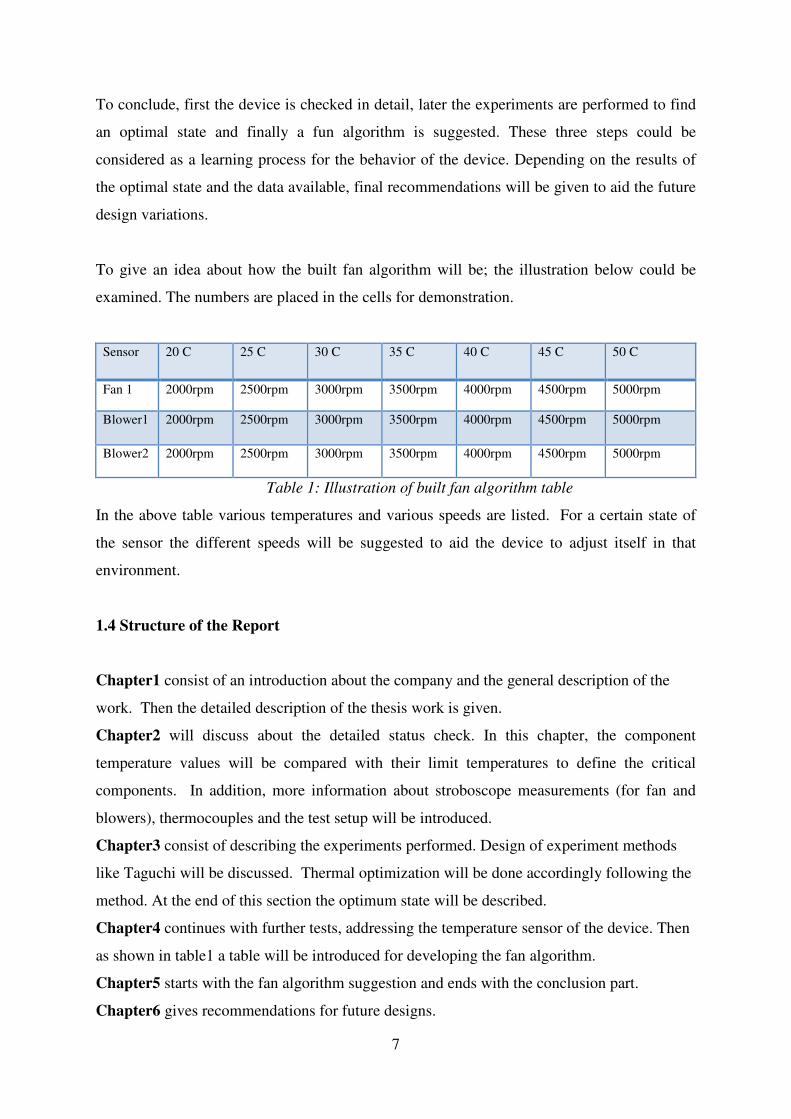
To give an idea about how the built fan algorithm will be; the illustration below could be
examined. The numbers are placed in the cells for demonstration.
Sensor 20 C 25 C 30 C 35 C 40 C 45 C 50 C
Fan 1 2000rpm 2500rpm 3000rpm 3500rpm 4000rpm 4500rpm 5000rpm
Blower1 2000rpm 2500rpm 3000rpm 3500rpm 4000rpm 4500rpm 5000rpm
Blower2 2000rpm 2500rpm 3000rpm 3500rpm 4000rpm 4500rpm 5000rpm
Table 1: Illustration of built fan algorithm table
In the above table various temperatures and various speeds are listed. For a certain state of
the sensor the different speeds will be suggested to aid the device to adjust itself in that
environment.
1.4 Structure of the Report
Chapter1 consist of an introduction about the company and the general description of the
work. Then the detailed description of the thesis work is given.
Chapter2 will discuss about the detailed status check. In this chapter, the component
temperature values will be compared with their limit temperatures to define the critical
components. In addition, more information about stroboscope measurements (for fan and
blowers), thermocouples and the test setup will be introduced.
Chapter3 consist of describing the experiments performed. Design of experiment methods
like Taguchi will be discussed. Thermal optimization will be done accordingly following the
method. At the end of this section the optimum state will be described.
Chapter4 continues with further tests, addressing the temperature sensor of the device. Then
as shown in table1 a table will be introduced for developing the fan algorithm.
Chapter5 starts with the fan algorithm suggestion and ends with the conclusion part.
Chapter6 gives recommendations for future designs.
8
2 Detailed Status Check
2.1 Before the detailed status check
The steps to be taken before the detailed status check:
• The highest possible temperature values for the components are determined.
• From the list of components 50 of them are selected and the thermocouples
are attached to those components.
The highest possible temperature values for the components are listed. Listing is done by
mostly looking at the datasheets of the components and related documents with the help of
electronic engineer Yijun Zhao.
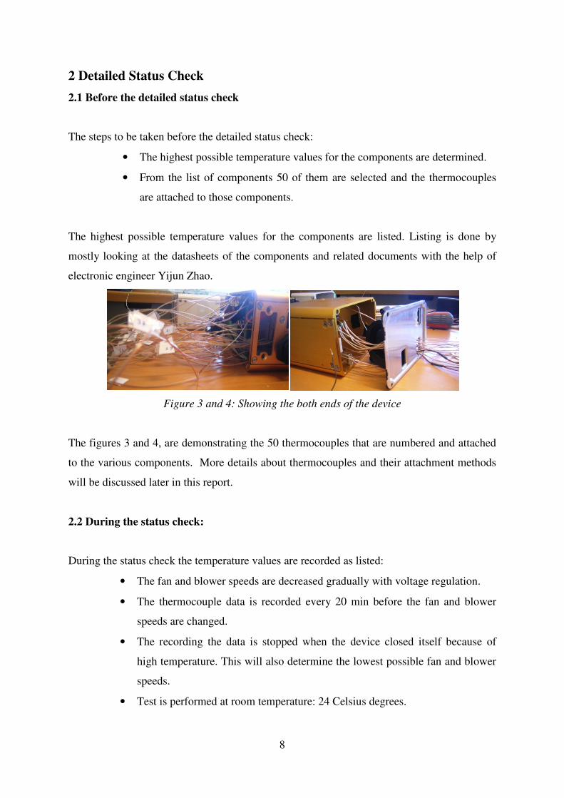
Figure 3 and 4: Showing the both ends of the device
The figures 3 and 4, are demonstrating the 50 thermocouples that are numbered and attached
to the various components. More details about thermocouples and their attachment methods
will be discussed later in this report.
2.2 During the status check:
During the status check the temperature values are recorded as listed:
• The fan and blower speeds are decreased gradually with voltage regulation.
• The thermocouple data is recorded every 20 min before the fan and blower
speeds are changed.
• The recording the data is stopped when the device closed itself because of
high temperature. This will also determine the lowest possible fan and blower
speeds.
• Test is performed at room temperature: 24 Celsius degrees.
9
It is also important to add that the speeds of fan and two different blowers are not identical to
each other and they have different values of rpm speed for the same voltage applied. To avoid
any misunderstanding it should be stated now that the all speeds are decreased gradually
during the status check. More information about the voltage regulation and related speeds
will be discussed later. [18]
2.3 After the detailed status check
The component temperature values are compared with their limit temperatures to define the
critical components. This is to choose the most important components to measure while
decreasing the number of thermocouples that are attached to unit.
The four graphs will be introduced related to the boards within the device. Remember that
there are two modules as named lamp module and main module. There are three electronic
boards in the main module and one in the lamp module. Ones that are in main module are
named pmd board, main board and the main power supply board. The one at the lamp module
is named ballast. Graphs will be shown to demonstrate how temperature values are compared
with their limit temperature values of the components.
The graphs’ titles have related board’s position and its location between the parentheses. On
vertical axis, temperature values are listed in Celsius degrees while horizontal axis the
numbered sensor values can be seen. At this stage, the speeds are given by their voltage
regulation percentage. The more information about the rpm values of fan and blower speeds
will be given later. In addition, every sensor number is representing one component.
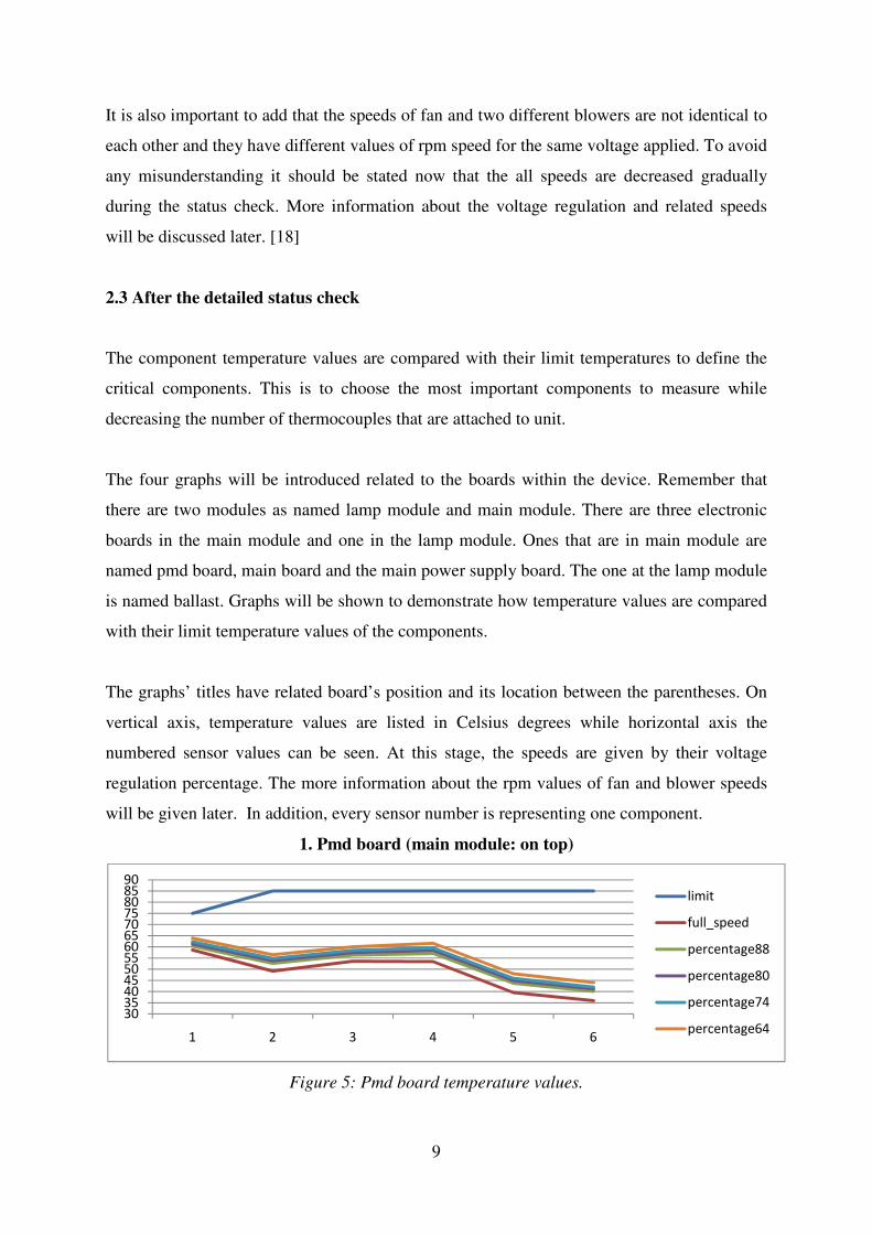
1. Pmd board (main module: on top)
Figure 5: Pmd board temperature values.
30354045505560657075808590
1 2 3 4 5 6
limit
full_speed
percentage88
percentage80
percentage74
percentage64
10
In figure 5, if we look at the blue line stated as limit is showing the upper most temperature
value a component can reach. Considering the limit on the graph, the numbered components
on the horizontal axis should not exceed the top blue line. In addition, it could be seen that, as
the speeds are decreasing the temperature values are increasing.
With this representation on the graph, the component temperature could be checked if it is
within its operating temperature values. At this point, we could see that in figure 5, the
component numbered with sensor 1 has almost 10 degrees Celsius to reach its limit
temperature (65 to 75). That’s why we should select that component as a critical component
for the further experiments.
Although, it is likely to be seen that there is always a gap between the limit values and the
component temperatures in this graph, we could not decrease the speeds of the fan and
blowers because the detailed status check is stopped when the device closed itself. The
device is closing itself when some components are exceeding a temperature value. However,
it is not certain when the device is closing itself since the related components and the highest
limit temperature value is not given. But we could make an assumption considering the four
graphs at the end of this section.
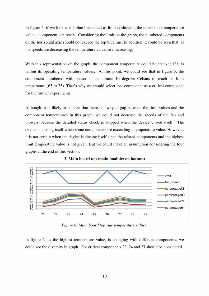
2. Main board top (main module: on bottom)
Figure 6: Main board top side temperature values.
In figure 6, as the highest temperature value, is changing with different components, we
could see the diversity in graph. For critical components 23, 24 and 27 should be considered.
3035404550556065707580859095
21 22 23 24 25 26 27 28 29
limit
full_speed
percentage88
percentage80
percentage74
percentage64
11
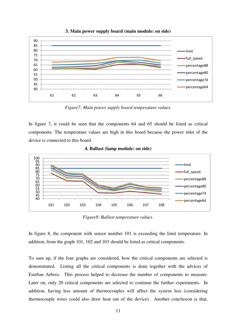
3. Main power supply board (main module: on side)
Figure7: Main power supply board temperature values.
In figure 7, it could be seen that the components 64 and 65 should be listed as critical
components. The temperature values are high in this board because the power inlet of the
device is connected to this board.
4. Ballast (lamp module: on side)
Figure8: Ballast temperature values.
In figure 8, the component with sensor number 101 is exceeding the limit temperature. In
addition, from the graph 101, 102 and 103 should be listed as critical components.
To sum up, if the four graphs are considered, how the critical components are selected is
demonstrated. Listing all the critical components is done together with the advices of
Esteban Arboix. This process helped to decrease the number of components to measure.
Later on, only 20 critical components are selected to continue the further experiments. In
addition, having less amount of thermocouples will affect the system less (considering
thermocouple wires could also draw heat out of the device). Another conclusion is that,
40
45
50
55
60
65
70
75
80
85
90
61 62 63 64 65 66
limit
full_speed
percentage88
percentage80
percentage74
percentage64
404550556065707580859095
100
101 102 103 104 105 106 107 108
limit
full_speed
percentage88
percentage80
percentage74
percentage64

12
depending on the fourth graph, the ballast board is closing the device when some of its
components are exceeding 85 Celsius degrees. More temperature readings considering the
other components are listed within the inner documents of Optea AB. [18]
2.4 Equipments that are used
Equipments that are used will be described in following section. Describing will be done by
giving information about their usage in the project and their working principle. Finally, the
test setup will be introduced before starting the other chapter about design of experiments.
List of equipments to be described:
• Stroboscope and rpm measurements
• Thermocouples and heat measurements
• Sound level meter and noise measurements
• Data logger
• Minitab software and I2C analyzer
2.4.1 Stroboscope and rpm measurements
A digital stroboscope is used to measure the rpm (rotation per minute) values of the fan and
blower. The stroboscope has two common usages one is to stop the motion for inspection
purposes and another one is to measure the speed. For measuring the speed, it needs a
reference point. In a symmetrical object like fan or blower a small reflective tape is used.
The rpm values are measured:
• To determine the rpm (rotation per minute) speeds for fan and two blowers.
• To check the stall (unexpected stop of rotation). Stall condition should be
avoided while performing voltage regulation.
Fan and blowers need a start up voltage to start up the rotation. However, sometimes the
given power is not enough for the engine load to keep on the rotation and as a result stall
occurs. To avoid the stall condition, the rotational speed examined with a stroboscope.
13
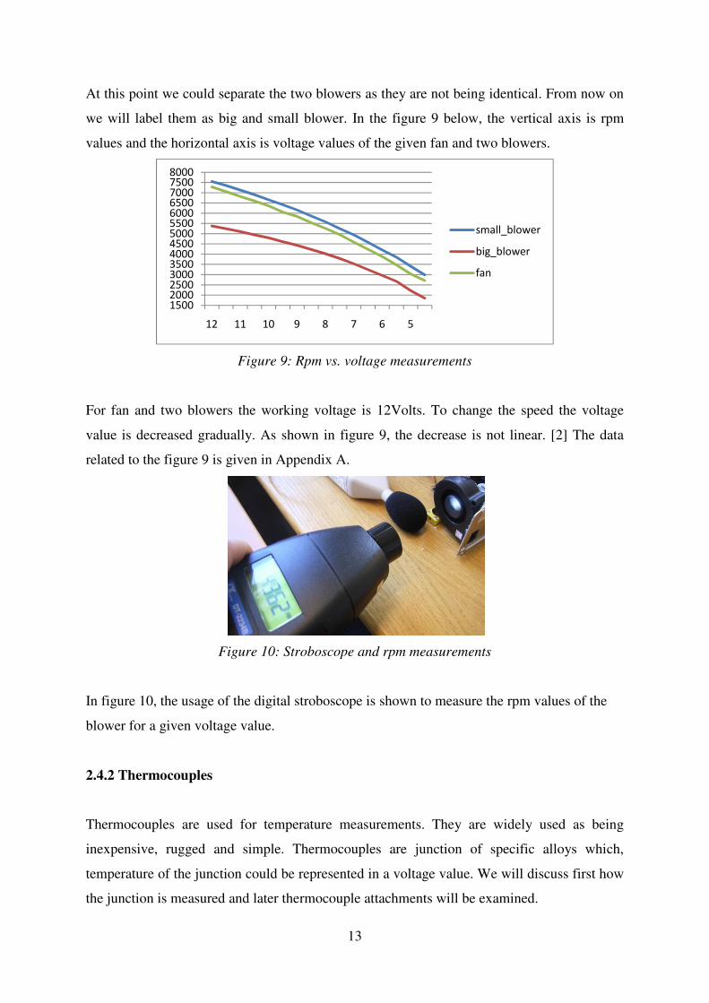
At this point we could separate the two blowers as they are not being identical. From now on
we will label them as big and small blower. In the figure 9 below, the vertical axis is rpm
values and the horizontal axis is voltage values of the given fan and two blowers.
Figure 9: Rpm vs. voltage measurements
For fan and two blowers the working voltage is 12Volts. To change the speed the voltage
value is decreased gradually. As shown in figure 9, the decrease is not linear. [2] The data
related to the figure 9 is given in Appendix A.
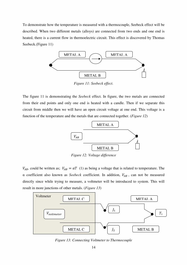
Figure 10: Stroboscope and rpm measurements
In figure 10, the usage of the digital stroboscope is shown to measure the rpm values of the
blower for a given voltage value.
2.4.2 Thermocouples
Thermocouples are used for temperature measurements. They are widely used as being
inexpensive, rugged and simple. Thermocouples are junction of specific alloys which,
temperature of the junction could be represented in a voltage value. We will discuss first how
the junction is measured and later thermocouple attachments will be examined.
15002000250030003500400045005000550060006500700075008000
12 11 10 9 8 7 6 5
small_blower
big_blower
fan
14
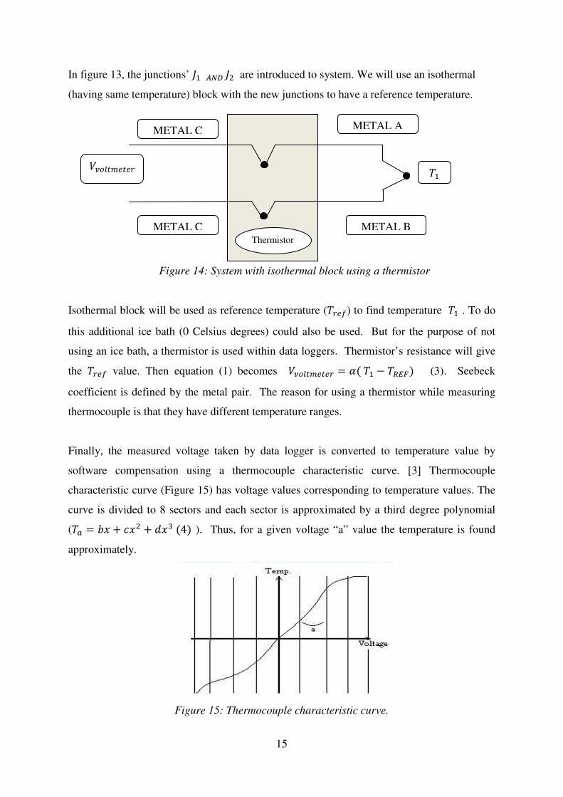
To demonstrate how the temperature is measured with a thermocouple, Seebeck effect will be
described. When two different metals (alloys) are connected from two ends and one end is
heated, there is a current flow in thermoelectric circuit. This effect is discovered by Thomas
Seebeck.(Figure 11)
Figure 11: Seebeck effect.
The figure 11 is demonstrating the Seebeck effect. In figure, the two metals are connected
from their end points and only one end is heated with a candle. Then if we separate this
circuit from middle then we will have an open circuit voltage at one end. This voltage is a
function of the temperature and the metals that are connected together. (Figure 12)
Figure 12: Voltage difference
���, could be written as; ��� � �� (1) as being a voltage that is related to temperature. The
α coefficient also known as Seebeck coefficient. In addition, ��� , can not be measured
directly since while trying to measure, a voltmeter will be introduced to system. This will
result in more junctions of other metals. (Figure 13)
Figure 13: Connecting Voltmeter to Thermocouple
Voltmeter
METAL A METAL A
METAL B
METAL A
METAL B
���
METAL A
METAL B
���� � �
METAL C
METAL C ��
�� ��
15
In figure 13, the junctions’ �� ��� �� are introduced to system. We will use an isothermal
(having same temperature) block with the new junctions to have a reference temperature.
Figure 14: System with isothermal block using a thermistor
Isothermal block will be used as reference temperature (�� �) to find temperature �� . To do
this additional ice bath (0 Celsius degrees) could also be used. But for the purpose of not
using an ice bath, a thermistor is used within data loggers. Thermistor’s resistance will give
the �� � value. Then equation (1) becomes ���� � � � �� �� � ����� (3). Seebeck
coefficient is defined by the metal pair. The reason for using a thermistor while measuring
thermocouple is that they have different temperature ranges.
Finally, the measured voltage taken by data logger is converted to temperature value by
software compensation using a thermocouple characteristic curve. [3] Thermocouple
characteristic curve (Figure 15) has voltage values corresponding to temperature values. The
curve is divided to 8 sectors and each sector is approximated by a third degree polynomial
(�� � �� � ��� � �! �4� ). Thus, for a given voltage “a” value the temperature is found
approximately.
Figure 15: Thermocouple characteristic curve.
METAL A
METAL B
METAL C
METAL C Thermistor
�� ���� � �
16
2.4.2.1 Thermocouple attachment
In previous section, how data logger measures the temperature is described. In this section
thermocouple attachment will be discussed with detail.
While doing measurements, the selected thermocouple should be placed carefully on top of
the component. The separation point of the two branches (thermocouple) is the point that the
measurement is taken. Thus, the separation point should be in contact with the component. If
there is not any direct contact with the component then there is a possibility that the
temperature of the airflow could be measured. In addition, as thermocouple wires being
conductive, they should be replaced to avoid any short circuit. A loose thermocouple wire
could harm the measuring device and the electronic board that the measure is taken. In
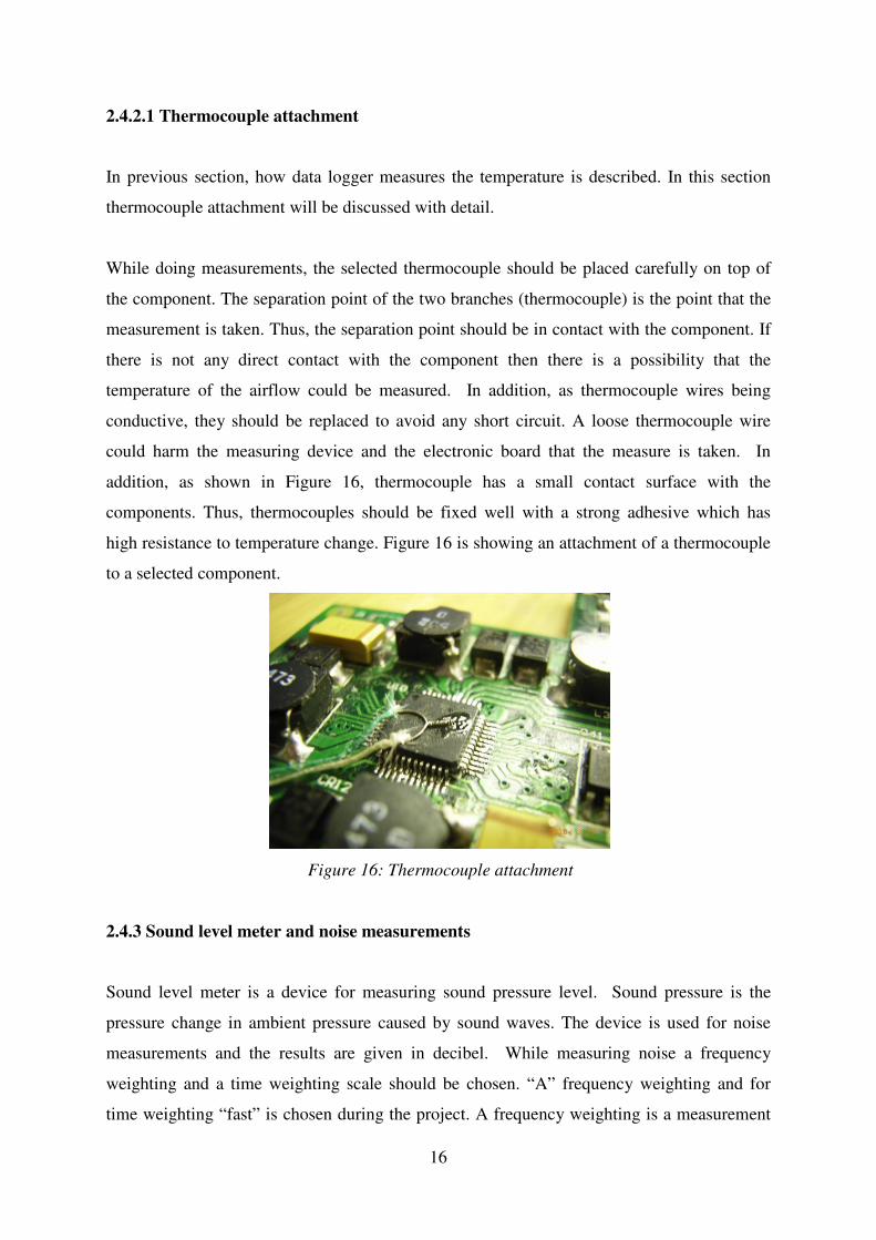
addition, as shown in Figure 16, thermocouple has a small contact surface with the
components. Thus, thermocouples should be fixed well with a strong adhesive which has
high resistance to temperature change. Figure 16 is showing an attachment of a thermocouple
to a selected component.
Figure 16: Thermocouple attachment
2.4.3 Sound level meter and noise measurements
Sound level meter is a device for measuring sound pressure level. Sound pressure is the
pressure change in ambient pressure caused by sound waves. The device is used for noise
measurements and the results are given in decibel. While measuring noise a frequency
weighting and a time weighting scale should be chosen. “A” frequency weighting and for
time weighting “fast” is chosen during the project. A frequency weighting is a measurement
17
that gives a close response of human hearing and giving the results in dbA. [4] First
additional information about absolute and relative measurements will be given. Second, some
details about the measuring conditions will be discussed.
First, we should discuss relative and absolute measurements of noise. For relating the
measurements to human hearing, absolute measurements are made. Decibels are relative
measurements but measurements are examined in levels relative to some random level. That
level then is selected 0dB and later measurements referenced to this level. In addition, for
noise measurements, lowest sound that can be detectable by human is selected as 0 dB. For
instance 40-45 dB is typical home residence. [4][5] (Appendix B for more examples)
Second, while measurements are taken the position of the sound level meter should be fixed
in a certain position. This is because the other elements could easily introduce noise to the
measurement. We can list the other noise elements (making noise while working) such as;
computer, data logger, power supply should also be in a fixed position. In additional window
and door could easily introduce additional noises to the system such as train passing outside
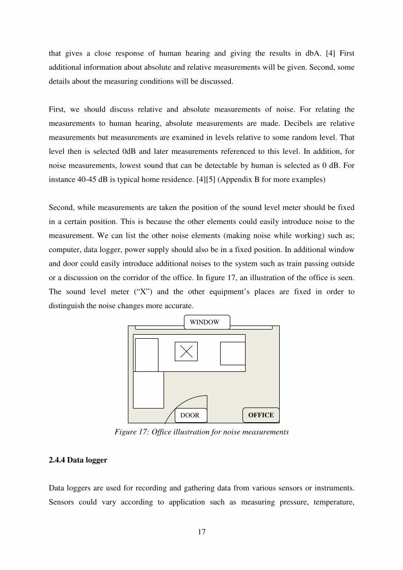
or a discussion on the corridor of the office. In figure 17, an illustration of the office is seen.
The sound level meter (“X”) and the other equipment’s places are fixed in order to
distinguish the noise changes more accurate.
Figure 17: Office illustration for noise measurements
2.4.4 Data logger
Data loggers are used for recording and gathering data from various sensors or instruments.
Sensors could vary according to application such as measuring pressure, temperature,
DOOR
WINDOW
OFFICE

18
vibration and more. In this project, Agilent data logger 34970A model is used with a 20
channel (one channel could take one sensor) 34901A module.
Figure 18 and 19: Data logger and thermocouple attached device
In figure 18 and 19, a picture of the data logger is given to demonstrate how the temperature
measurements are taken. In addition in the left figure it could be seen that each thermocouple
is numbered with white stickers. More pictures about how thermocouples are connected to
data logger Appendix C could be examined with Agilent Data logger user manual [6].
2.4.5 Minitab Software
Minitab is statistical software to analyse data (thermocouple readings in our case). Minitab is
used for improving quality and to shorten the time for analyses of data for various projects.
[7] In this project Minitab program, is used to construct orthogonal arrays (list of
experiments) and show mean plot analyses for Taguchi method (DOE). Orthogonal arrays
and mean plot analyses will be explained together with the Taguchi method in detail later at
chapter 3.
2.4.6 I2C Analyzer
This device is used for gathering the temperature sensor (Digital temperature sensor with I2C
interface) data from the device. The temperature sensor within the device is shown in
Figure2 in green colour. This data later will be used as a reference to develop Fan algorithm.
In addition, the sensor readings are on hexadecimal values and they are converted to decimal
values. (For conversion of temperature values see Appendix E.)

19
2.5 Short List of the tools
• Thermocouples: K type-TT-K-30 (Neoflon PFA insulated). Red: low yellow: high
Type K (see Appendix D) is selected because of its common usage and suitable price.
The diameter of the thermocouple cable is tried to be selected small considering
assembly of the unit.
• Adhesive: Loctite 401-instant adhesive is selected with a suitable accelerator.
Instant-adhesive selected considering small surface contact and temperature
resistance.
• Data logger: Agilent 34970A data logger – with module (34901A - 20 channels).
Agilent 34970A data logger selected for suitable price and quality.
• Sound level meter: A frequency weighting dB(A). “Fast” time weighting mode
selected during the experiments.
• Minitab: Student version is used for Taguchi (DOE) analyses.
• I2C analyzer: Beagle I2C/ SPI protocol analyzer used. [19]
2.6 Test Setup
In this section, how the equipments are placed and connected to each other will be discussed.
Demonstration will be done by pictures and the illustrations that are given.
Figure 20: Data logger- projector box and the power supplies
In figure 20, data logger (on left most), the wooden box (next to data logger) for the device
and the power supplies (on right most) are shown. Wooden box is build for getting more
accurate noise measurements. Inside the box the sound level meter is in a fixed position. In
addition, different power supplies (on right most) are used for powering the device and
manipulating (voltage regulation) the air units (fan and two blowers).

20
Figure 21, 22, and 23: The projector with rubber cover inside the box, inside the box and the
sound level meter.
In figure 21 (left most) and 22(middle), inside of the wooden box is shown with the fixed
position of the sound level meter. In addition it could be seen that the box is covered with egg
cartoons to lower the external noise. In figure 23(right most), the sound level meter is shown.
Figure 24: Illustration of the devices in the office.
Figure 24 is slightly changed version of figure 17. Letters are symbolising different
equipments that is used and their fixed location. D is symbolizing the data logger. C is
symbolising the project computer. P is symbolising power supplies. X is symbolising the
device (projector) in the wooden box.
Figure 25: Connections of the equipments.
In figure 25, the connections are demonstrated. Device is connected to data logger with
thermocouple sensors and to computer with I2C data analyzer. Power supplies are connected
D P
C
X
DOOR
WINDOW
OFFICE
Computer
Data logger Box with
device
Power
supplies
21
to fan, two blowers and the power inlet of the projector. Data logger is connected to the
project computer.
2.7 Summary
In this chapter, detailed status check is examined together with the selection of critical
components. Critical component selection is done by comparing component temperature
values with their limit temperatures. Later, more information about various equipments is
given such as stroboscope measurements, thermocouples, data logger, and sound lever meter.
Finally, the test setup is introduced and described with illustrations. In next chapter selected
critical components and test setup will be used with various experiments. How the
experiments constructed will be described in detail.
3 Experiments
3.1 Introduction to Experiments
Experiments are done to discover information about a process or a system. Information
gathered could be used to improve the process. Thus, well constructed and planned
experiments are needed to have consistent outputs for the changes made during the
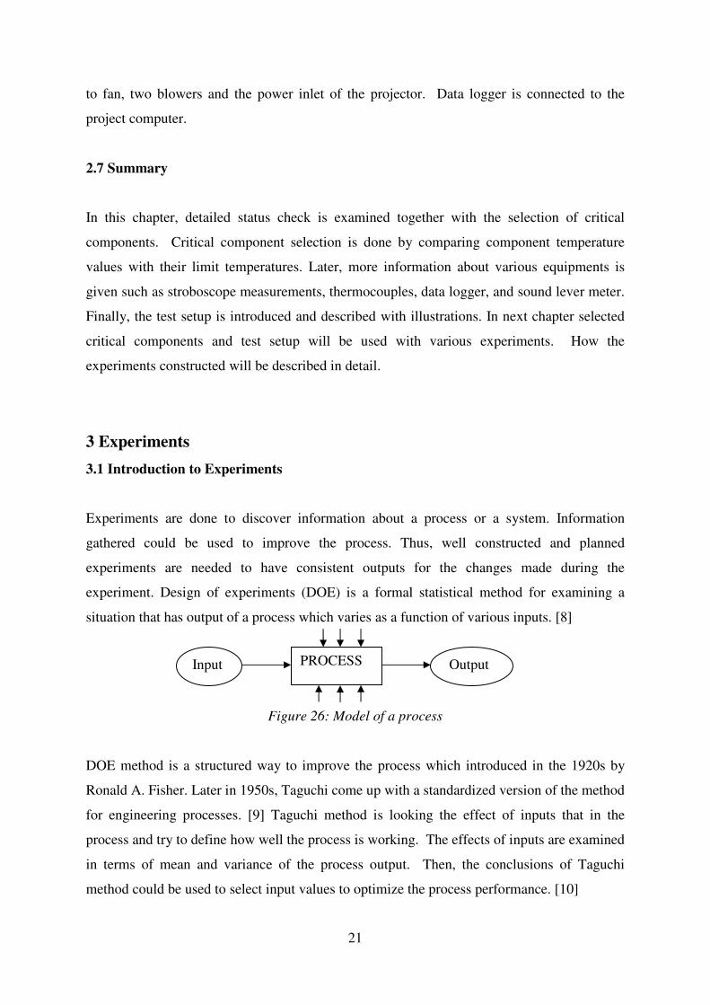
experiment. Design of experiments (DOE) is a formal statistical method for examining a
situation that has output of a process which varies as a function of various inputs. [8]
Figure 26: Model of a process
DOE method is a structured way to improve the process which introduced in the 1920s by
Ronald A. Fisher. Later in 1950s, Taguchi come up with a standardized version of the method
for engineering processes. [9] Taguchi method is looking the effect of inputs that in the
process and try to define how well the process is working. The effects of inputs are examined
in terms of mean and variance of the process output. Then, the conclusions of Taguchi
method could be used to select input values to optimize the process performance. [10]
PROCESS Input Output
22
3.2 Taguchi method:
Taguchi method in general:
• Taguchi method is using orthogonal arrays (i.e. balanced list of experiments.)
to examine the variation of inputs on the process
• Instead of listing all the variables (inputs) and testing all the combinations,
Taguchi method looks at some pairs of combinations to gather up information
about the process.
• Taguchi method is aiming to do minimum number of experimentation for
improving the quality of the process.
• The arrays (i.e. list of experiments) for Taguchi method are selected based on
the number of parameters (input) and the state of the inputs (levels).
Taguchi method is using balanced list of experiments (orthogonal arrays) in order to
manipulate the levels of inputs. [10] We could consider a simple example for illustrating
levels, inputs and arrays. In that example cook is making bread with flour, water and yeast,
which are the also the inputs of the system while the amount of that each ingredient is the
level of that corresponding input. If there is a selection between 200ml of water and 400ml of
water during experiments, we could take it as “input water” has two levels. In this example, if
we have two levels for each three input, then for all combinations the number of total
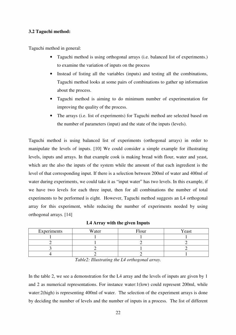
experiments to be performed is eight. However, Taguchi method suggests an L4 orthogonal
array for this experiment, while reducing the number of experiments needed by using
orthogonal arrays. [14]
L4 Array with the given Inputs
Experiments Water Flour Yeast
1 1 1 1
2 1 2 2
3 2 1 2
4 2 2 1
Table2: Illustrating the L4 orthogonal array.
In the table 2, we see a demonstration for the L4 array and the levels of inputs are given by 1
and 2 as numerical representations. For instance water:1(low) could represent 200ml, while
water:2(high) is representing 400ml of water. The selection of the experiment arrays is done
by deciding the number of levels and the number of inputs in a process. The list of different
23
orthogonal arrays and array selectors could be found on World Wide Web or various Taguchi
books. For a small array selector matrix example, see Appendix F.
Analyses of Taguchi method could be done by mean and variance analyses. The mean
analysis is calculated as comparing the effects of different inputs. [11]
Average output value when input: A is high = X (1)
Average output value when input: A is low = Y (2)
Effect of A= X-Y from (1) and (2)
When compared with the other inputs of the process, the effect value indicates which input
has more effect on the process. The effect values could be easily compared by looking at the
slope of the mean plots. [11] Depending on the slopes the effects are compared. If the slope is
high, the effect is higher as a result. Then, different levels from different inputs are selected
for satisfying the given output values. The conclusion of selected set of experiments, could
lead to a new set of experiments based on the previous selection, which is also known as
“Iterative Taguchi” method. [12] As seeing the design of experiments as a learning process
the conclusions of experiments that are leading to new experiments is suggesting that
experimentation is iterative. [13]
In this project, Iterative Taguchi method will be used to find the optimal solution for the
projector with mean plot analyses. The conclusions and explanations of the selecting
parameters (inputs) will be given in next section.
3.3 Implementing Taguchi method for the project
The corresponding inputs and outputs should be selected. Depending on the experiments
goal, the outputs to examine and inputs to manipulate could change. Thus, the goal of the
experiment should be chosen.
As in this project we could state that:
“The goal is decreasing the noise of the device, while focusing on keeping the temperature
values within the limits.”
After stating the goal, we could select the output variables to examine as noise and
temperature values. How the measurements taken are stated in the test setup in previous

24
chapter. In this point, the experimentation will continue at room temperature and at the built
in test setup for the measurements.
In addition to output variables (noise and temperature), the input variables are listed as:
• Fan: Speed
• Blower1(big): Speed
• Blower2(small): Speed
• Heat pads
• Rubber cover
The input variables are selected considering the most suitable changes could be done to the
device for available test conditions. The ambient pressure, position of the fan and blowers,
the environment temperature are neglected as inputs as the time and cost optimization of the
project.
Figure 27: Input, process and output
In figure 27 a short list of input process and outputs is shown. Figure 27 is also an illustration
of the figure 26 for this project. As various changes in the inputs applied, that will result in
change in the temperature and noise measurements.
To add more, there are various heat pads within the device to dissipate the heat out of the
system. Those heat pads are aimed to decrease the air gap between some components and the
device enclosure. Thus, heat pads are introducing a middle layer with high thermal
conductivity between the component and the enclosure. While reducing the heat from certain
components, this could result in high temperatures for the touch temperature of the device.
Another point is since there is air flow within the device putting heat pads may not be
effective as using the fan and blowers.
In addition, since the experiments are planning to reduce the fan and blower speeds for
decreasing noise. The decreasing the speeds could raise the touch temperature of the device.
Device
(process)
Noise(output)
Temperature
(output)
Fan and blowers speed
(input)
Heat pads (input)
Rubber cover(input)

25
The enclosure temperature could reach its limit which is 46 degrees Celsius for avoiding skin
burns when touched.[15] Thus, adding a rubber cover could solve the problem for exceeding
temperatures for enclosure and help to keep the temperature inside of the device since rubber
has low thermal conductivity coefficient than the aluminium device enclosure. However, this
could result in higher temperature values within the device.
To sum up, while examining the results of the experiments, we will try to conduct solutions
for the various outcomes of the process. As experiments applied for the device, we will try to
find an optimal solution as analysing the experimental data.
Selection of levels for the inputs:
• Rubber cover for lamp module with/without
• Heat pads with / without
• Fan: slow(5259rpm) 2: middle(6355rpm ) 3:fast(7286rpm)
• Blower big: 1:slow(4018rpm) 2:middle(4798rpm ) 3:fast(5375rpm)
• Blower small: 1:slow(5580rpm) 2:middle(6658rpm ) 3:fast(7546rpm)
Since there are various ways to put heat pads or rubber cover, most suitable variations are
selected for the levels. For rubber cover position, the top of lamp module enclosure is
selected due to high heat generation from the lamp module. For heat pads, the effect on the
components when there is no heat pads will be examined. While examining the heat pads, the
variation of heat pad positions will be neglected due to high time consumption of the process.
Fan and blowers speed range is divided into three categories as being slow, medium and fast.
The lowest limit speed is selected considering the status check of the device.
To summarize, until now we selected the inputs, input levels and defined the outputs of the
system. Together with the critical components in status check, fan and blower temperature
values are also going to be examined. As having five inputs and various levels (two and
three) the experiments will be done in three iterative runs. This is to have more control over
the experiments and trying to get more information from the process. These three runs are
implemented as selecting and manipulating the orthogonal arrays while the levels of the
inputs are depending on the previous run (as being iterative).
26
When having different levels or having fewer inputs for a selected experiment array. The
array manipulation could be applied. Manipulating the orthogonal arrays could be done by
two methods. First by omitting a column, if there are not many inputs in the experiment for
the selected array.[16] Second, if the levels of an input vary, then the input column that has
less levels could be changed randomly to adjust the number of levels.[10][16]
In the next section, the iterative experimental runs are described. The input levels and the
arrays are selected and the results will be examined with the mean plots. The conclusions of
the next section will lead us to the optimal solution for the system.
3.4 Experimental runs
3.4.1 Introduction
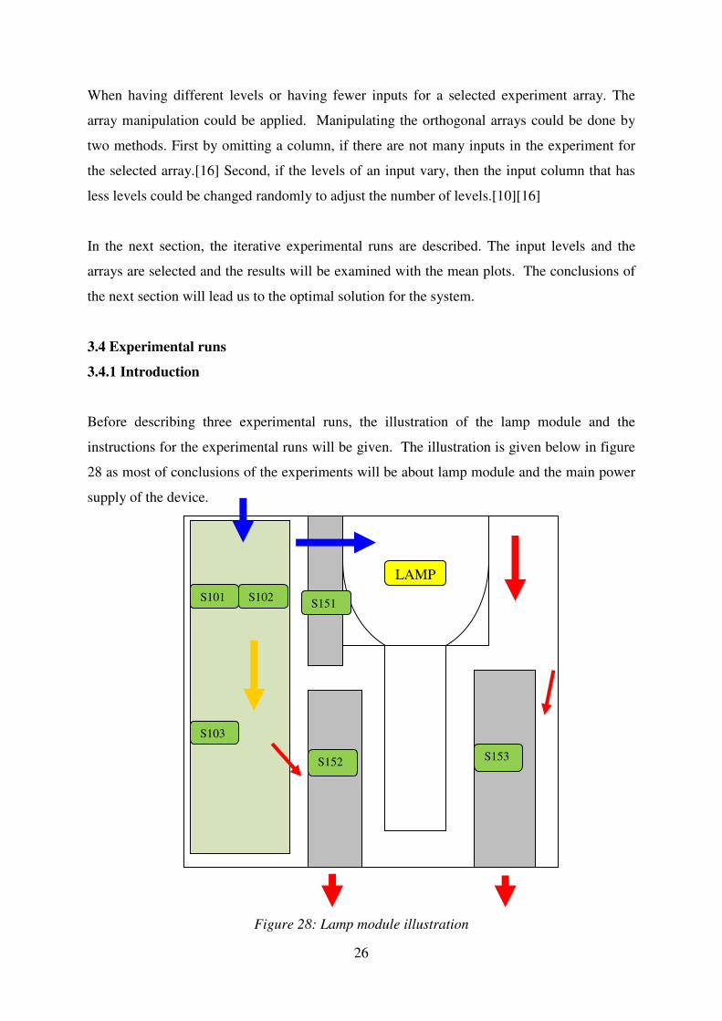
Before describing three experimental runs, the illustration of the lamp module and the
instructions for the experimental runs will be given. The illustration is given below in figure
28 as most of conclusions of the experiments will be about lamp module and the main power
supply of the device.
Figure 28: Lamp module illustration
S101 S102
S103
S151
S152 S153
LAMP
27
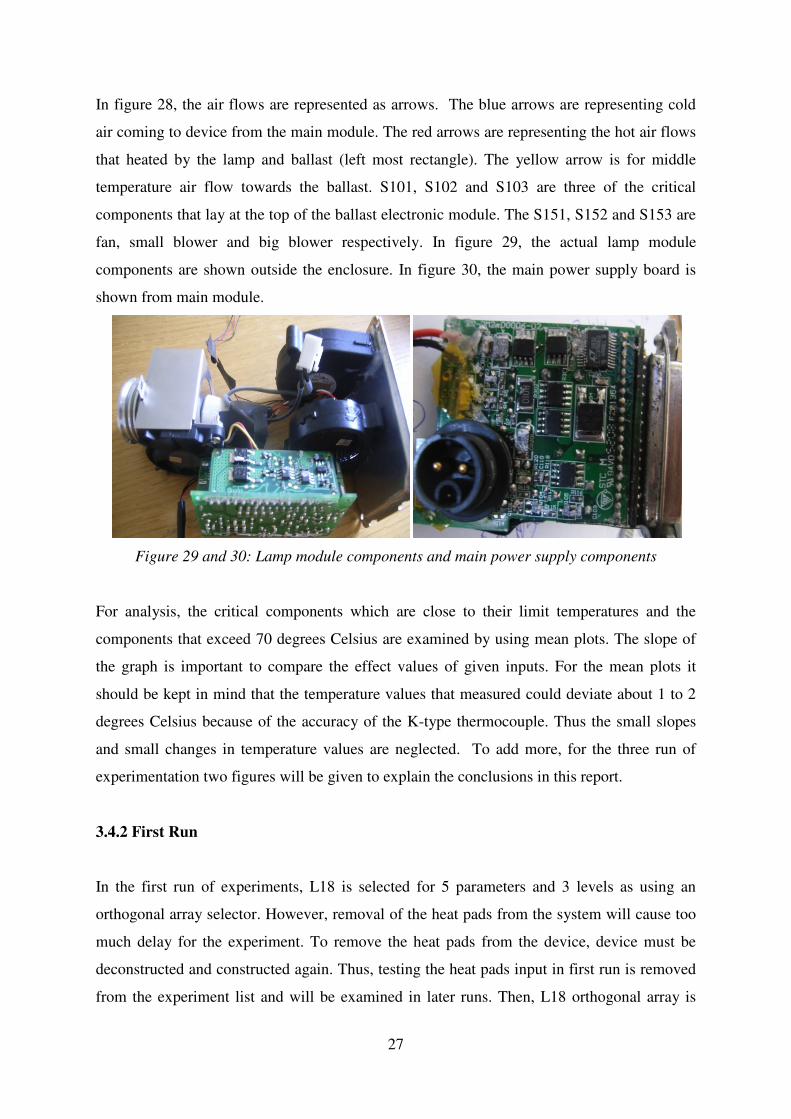
In figure 28, the air flows are represented as arrows. The blue arrows are representing cold
air coming to device from the main module. The red arrows are representing the hot air flows
that heated by the lamp and ballast (left most rectangle). The yellow arrow is for middle
temperature air flow towards the ballast. S101, S102 and S103 are three of the critical
components that lay at the top of the ballast electronic module. The S151, S152 and S153 are
fan, small blower and big blower respectively. In figure 29, the actual lamp module
components are shown outside the enclosure. In figure 30, the main power supply board is
shown from main module.
Figure 29 and 30: Lamp module components and main power supply components
For analysis, the critical components which are close to their limit temperatures and the
components that exceed 70 degrees Celsius are examined by using mean plots. The slope of
the graph is important to compare the effect values of given inputs. For the mean plots it
should be kept in mind that the temperature values that measured could deviate about 1 to 2
degrees Celsius because of the accuracy of the K-type thermocouple. Thus the small slopes
and small changes in temperature values are neglected. To add more, for the three run of
experimentation two figures will be given to explain the conclusions in this report.
3.4.2 First Run
In the first run of experiments, L18 is selected for 5 parameters and 3 levels as using an
orthogonal array selector. However, removal of the heat pads from the system will cause too
much delay for the experiment. To remove the heat pads from the device, device must be
deconstructed and constructed again. Thus, testing the heat pads input in first run is removed
from the experiment list and will be examined in later runs. Then, L18 orthogonal array is
28
adopted (manipulated) for 4 parameters and at most 3 levels by omitting columns from the
array. [16]
First run summary: L18 array with 4 parameters and most 3 levels.
• Fan rpm 1:slow(5259rpm) 2: middle(6355rpm ) 3:fast(7286rpm)
• Blower –small-rpm 1:slow(5580rpm) 2:middle(6658rpm ) 3:fast(7546rpm)
• Blower – big –rpm 1:slow(4018rpm) 2:middle(4798rpm ) 3:fast(5375rpm)
• Rubber cover: 1 : with 2:without
• Conclusion: Rubber cover should be selected with:1.
In summary part above, the parameters and their levels are shown for the experiment. The
conclusion will be discussed by given mean plot graphs.
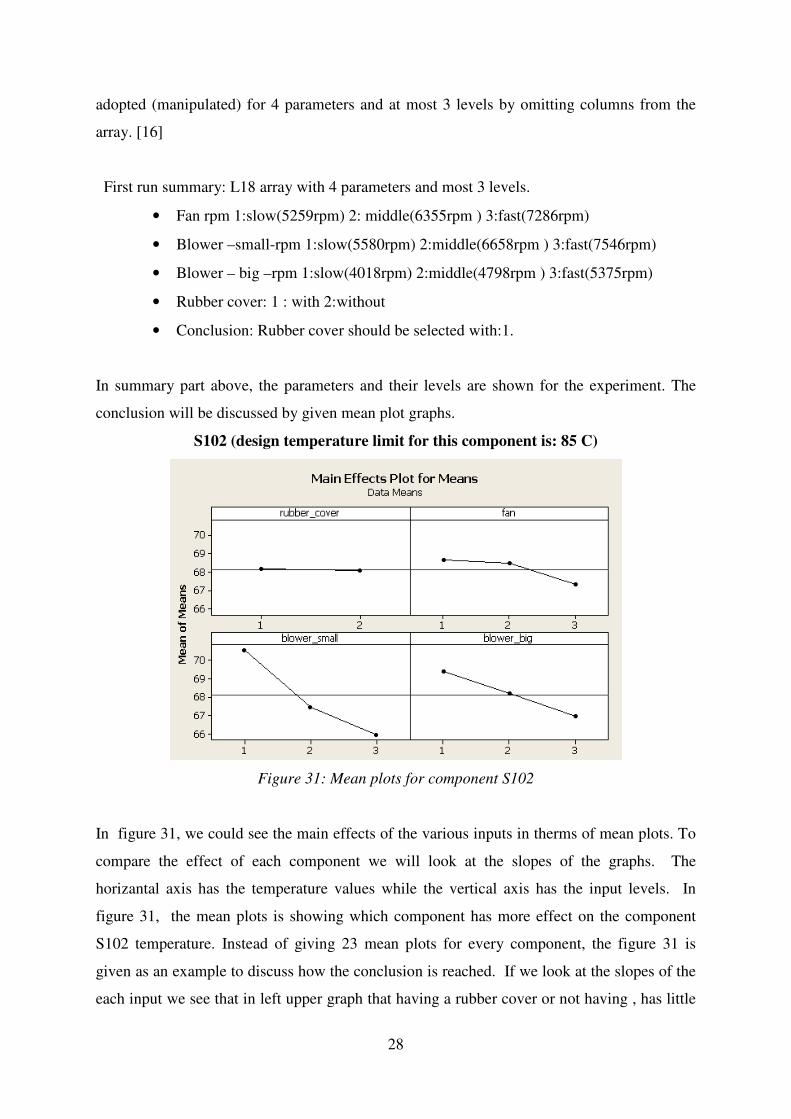
S102 (design temperature limit for this component is: 85 C)
Figure 31: Mean plots for component S102
In figure 31, we could see the main effects of the various inputs in therms of mean plots. To
compare the effect of each component we will look at the slopes of the graphs. The
horizantal axis has the temperature values while the vertical axis has the input levels. In
figure 31, the mean plots is showing which component has more effect on the component
S102 temperature. Instead of giving 23 mean plots for every component, the figure 31 is
given as an example to discuss how the conclusion is reached. If we look at the slopes of the
each input we see that in left upper graph that having a rubber cover or not having , has little
29
effect when compared to the blowers and fan speeds. Thus, we could conclude that when
compared fan and blowers has more effect on the system than the rubber cover. This will
also answer our question about rubber cover as showing having a rubber cover does not have
a high effect for the component temperatures. It is also important to note that the mean plots
could only be used to compare the input effects for a given output. The slopes would be
different with different inputs or levels. To add more, we could see that as the speeds of the
fan and blowers are increasing towards level-3 , the component temperature is decreasing.
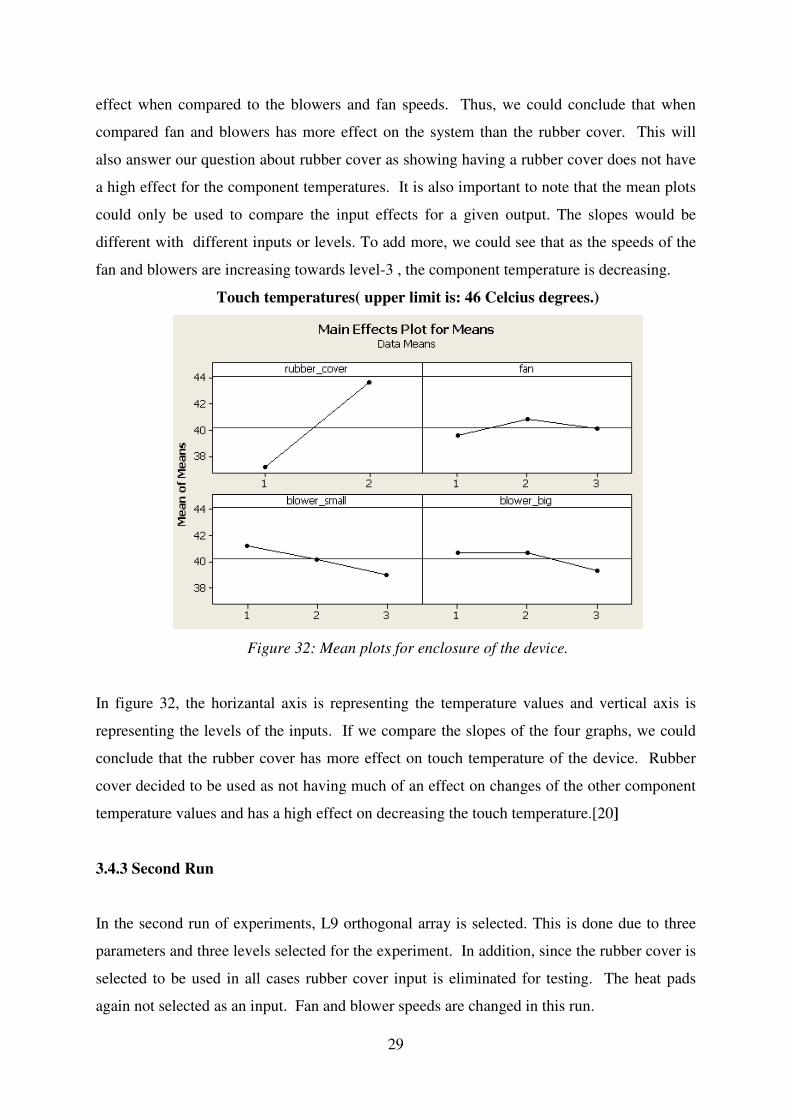
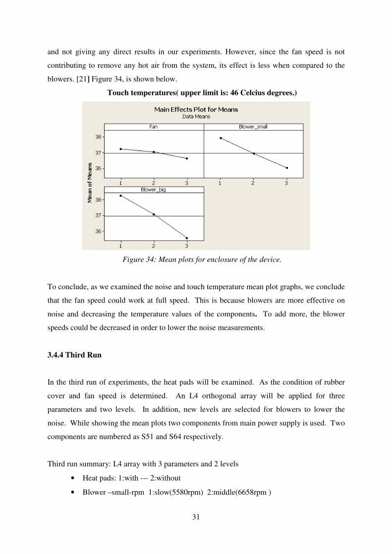
Touch temperatures( upper limit is: 46 Celcius degrees.)
Figure 32: Mean plots for enclosure of the device.
In figure 32, the horizantal axis is representing the temperature values and vertical axis is
representing the levels of the inputs. If we compare the slopes of the four graphs, we could
conclude that the rubber cover has more effect on touch temperature of the device. Rubber
cover decided to be used as not having much of an effect on changes of the other component
temperature values and has a high effect on decreasing the touch temperature.[20]
3.4.3 Second Run
In the second run of experiments, L9 orthogonal array is selected. This is done due to three
parameters and three levels selected for the experiment. In addition, since the rubber cover is
selected to be used in all cases rubber cover input is eliminated for testing. The heat pads
again not selected as an input. Fan and blower speeds are changed in this run.

30
Second run summary: L9 array with 3 parameters and 3 levels.
• Fan rpm 1:slow(5259rpm) 2: middle(6355rpm ) 3:fast(7286rpm)
• Blower –small-rpm 1:slow(5580rpm) 2:middle(6658rpm ) 3:fast(7546rpm)
• Blower – big –rpm 1:slow(4018rpm) 2:middle(4798rpm ) 3:fast(5375rpm)
• Conclusion: Fan speed should be selected fast(7286rpm).
In summary part above, the parameters and their levels are shown for the experiment. The
conclusion will be discussed by given mean plot graphs.
Noise
Figure 33: Mean plots for noise measurements of the device.
In figure 33, in vertical axis the dbA measurements for noise is shown. In horizantal axis, we
saw input levels for the experiment. By comparing the three graphs we could conclude that
the device’s noise is mostly effected by the blowers. Another outcome is that, the speeds of
blowers are increasing from level 1 to 3 the noise measurements are increasing too.
In figure 34, the vertical axis is representing the temperature values while horizantal axis is
the different levels of the input. If we examine three graphs we saw that the blowers has
more effect relative to the fan. While blowers speed is increasing from level 1 to 3, we see
that the touch temperature is decreasing. This is because more hot air is transferred out of the
system. Thus decreasing the temperature. For fan being less effective comparision to the
blowers we may consider that, the fan speed could be decreasing the temperature of the lamp
31
and not giving any direct results in our experiments. However, since the fan speed is not
contributing to remove any hot air from the system, its effect is less when compared to the
blowers. [21] Figure 34, is shown below.
Touch temperatures( upper limit is: 46 Celcius degrees.)
Figure 34: Mean plots for enclosure of the device.
To conclude, as we examined the noise and touch temperature mean plot graphs, we conclude
that the fan speed could work at full speed. This is because blowers are more effective on
noise and decreasing the temperature values of the components. To add more, the blower
speeds could be decreased in order to lower the noise measurements.
3.4.4 Third Run
In the third run of experiments, the heat pads will be examined. As the condition of rubber
cover and fan speed is determined. An L4 orthogonal array will be applied for three
parameters and two levels. In addition, new levels are selected for blowers to lower the
noise. While showing the mean plots two components from main power supply is used. Two
components are numbered as S51 and S64 respectively.
Third run summary: L4 array with 3 parameters and 2 levels
• Heat pads: 1:with --- 2:without
• Blower –small-rpm 1:slow(5580rpm) 2:middle(6658rpm )
32
• Blower – big –rpm 1:slow(4018rpm) 2:middle(4798rpm )
• Conclusion: Heat pads should be selected with.
In summary part above, the parameters and their levels are shown for the experiment. The
conclusion will be discussed by given mean plot graphs.
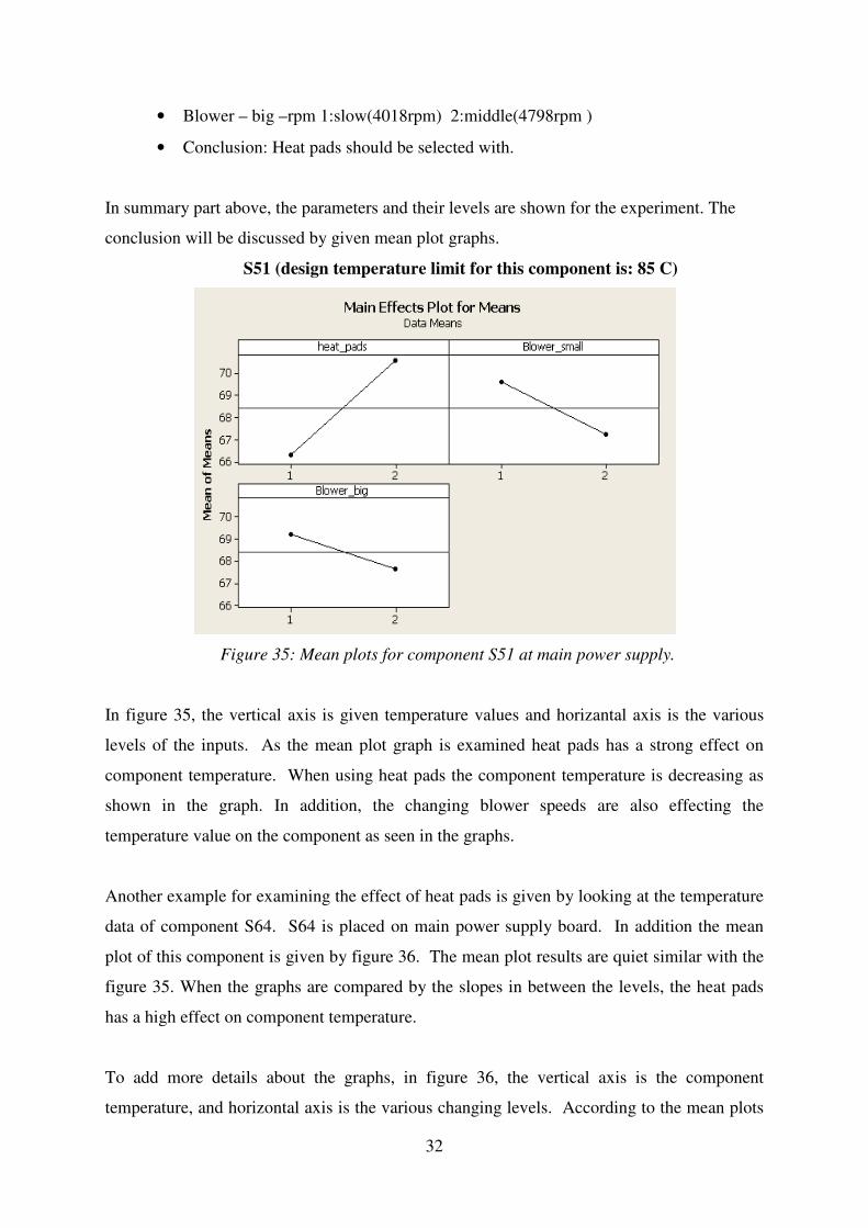
S51 (design temperature limit for this component is: 85 C)
Figure 35: Mean plots for component S51 at main power supply.
In figure 35, the vertical axis is given temperature values and horizantal axis is the various
levels of the inputs. As the mean plot graph is examined heat pads has a strong effect on
component temperature. When using heat pads the component temperature is decreasing as
shown in the graph. In addition, the changing blower speeds are also effecting the
temperature value on the component as seen in the graphs.
Another example for examining the effect of heat pads is given by looking at the temperature
data of component S64. S64 is placed on main power supply board. In addition the mean
plot of this component is given by figure 36. The mean plot results are quiet similar with the
figure 35. When the graphs are compared by the slopes in between the levels, the heat pads
has a high effect on component temperature.
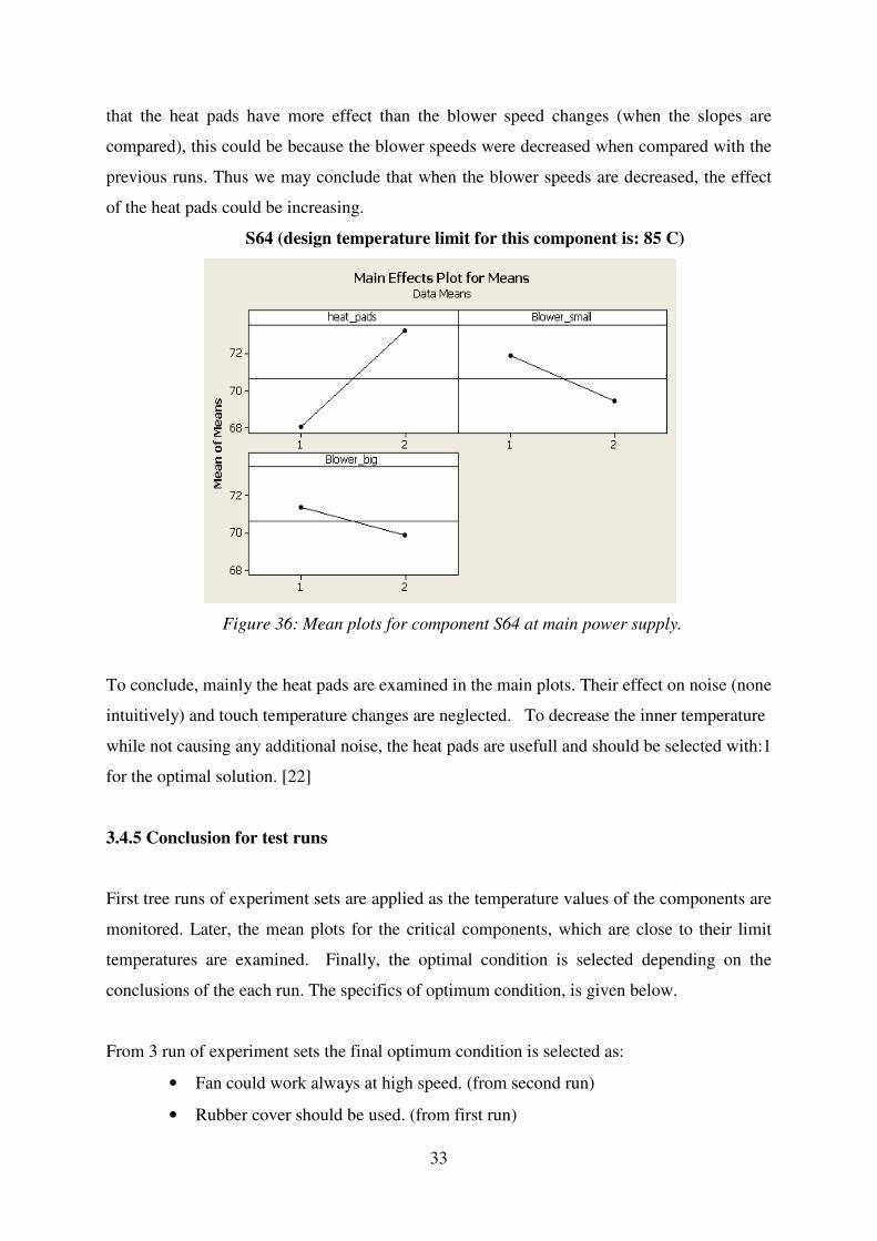
To add more details about the graphs, in figure 36, the vertical axis is the component
temperature, and horizontal axis is the various changing levels. According to the mean plots
33
that the heat pads have more effect than the blower speed changes (when the slopes are
compared), this could be because the blower speeds were decreased when compared with the
previous runs. Thus we may conclude that when the blower speeds are decreased, the effect
of the heat pads could be increasing.
S64 (design temperature limit for this component is: 85 C)
Figure 36: Mean plots for component S64 at main power supply.
To conclude, mainly the heat pads are examined in the main plots. Their effect on noise (none
intuitively) and touch temperature changes are neglected. To decrease the inner temperature
while not causing any additional noise, the heat pads are usefull and should be selected with:1
for the optimal solution. [22]
3.4.5 Conclusion for test runs
First tree runs of experiment sets are applied as the temperature values of the components are
monitored. Later, the mean plots for the critical components, which are close to their limit
temperatures are examined. Finally, the optimal condition is selected depending on the
conclusions of the each run. The specifics of optimum condition, is given below.
From 3 run of experiment sets the final optimum condition is selected as:
• Fan could work always at high speed. (from second run)
• Rubber cover should be used. (from first run)
34
• Heat pads should be used. (from third run)
• Blower speeds could vary.
However while examining the temperatures for the critical components (23 components), it is
monitored that the fan and blower temperature measurements are always higher than their
limit temperature (70 degrees Celsius.) This could be because the hot air they are trying to
circulate is heating them. In addition, the big blower temperatures are higher when compared
with the small blower and the fan. Various setups are tried to solve this problem however the
fan and blowers heat problem could not solved. [23] See Appendix G for the tried different
setups.
3.5 Summary
At the beginning of this chapter we introduced the Taguchi method. First, implementing the
Taguchi method is described. Later, selecting orthogonal arrays and input parameters
examined together with deciding on input levels and manipulating the orthogonal arrays.
Then, experimental runs are given with the mean plot analyses. Finally, the optimal solution
is given while introducing the fan and blowers heating problem.
4 Further Experiments
4.1 Introduction
In previous chapter the optimum state is defined as having rubber cover and heat pads while
fan is working at full speed. In addition, we added the blower speeds could vary. In this
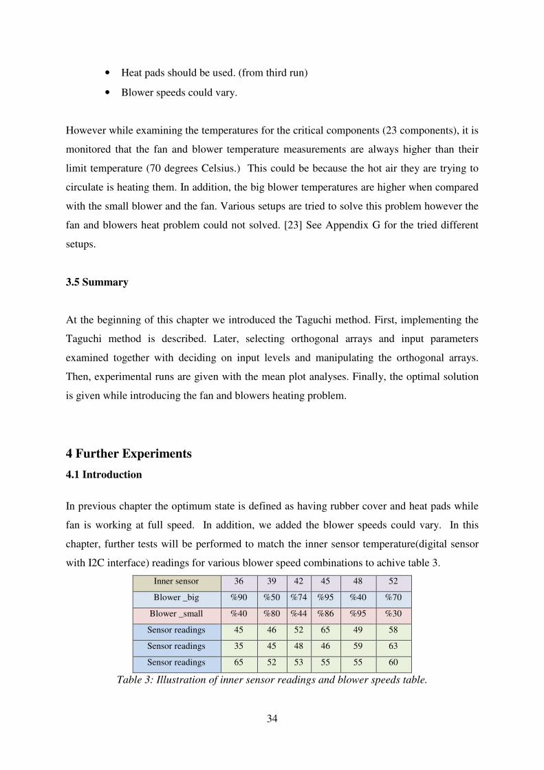
chapter, further tests will be performed to match the inner sensor temperature(digital sensor
with I2C interface) readings for various blower speed combinations to achive table 3.
Inner sensor 36 39 42 45 48 52
Blower _big %90 %50 %74 %95 %40 %70
Blower _small %40 %80 %44 %86 %95 %30
Sensor readings 45 46 52 65 49 58
Sensor readings 35 45 48 46 59 63
Sensor readings 65 52 53 55 55 60
Table 3: Illustration of inner sensor readings and blower speeds table.
35
In table 3, an illustration is given to show how the temperature readings are matched with the
blower speeds. After performing the absolute test a table similar to table 3 will be given. In
the corresponding table, the blower speeds will be given also by percentage of power since
the blowers are not being identical, writing the corresponding speed will not give
information, if the speed is decreased or increased. As in table 3, the inner temperature
readings will be divided to 5 or 6 levels among each other to represent the different states.
In additional, the experiments for matching the inner temperature reading and the various
blower speeds will be referred as absolute tests. Before performing the absolute tests to
construct the table, a status check will be constructed to test the optimal condition. This will
be done also to see the lowest blower speeds possible in optimal condition that is defined
previous chapter. [24] The status check is performed by decreasing the blower speeds
gradually until the device closes itself.
4.2 Status check and absolute test
In the status check, 4 different speeds are selected for each blower to test the all combinations
in absolute test. While testing the 16 combinations the inner temperature sensor values are
recorded to match the data. [25] Together with status check and the tested 16 combinations
there occur a table of 20 level-states with different combinations of the speeds. [26] Among
those 20 level-states, 5 of them are selected to construct the table illustrated by table 3. The
constructed table is on table 4. For the full table, with sensor readings see Appedix H. [27]
4.3 Selection of levels
The selection of 5 levels are done by considering:
• the limit temperatures of the critical components
• fan and blower over-heating problem
• blowers are not being identical
• inner temperature sensor(digital sensor) readings
• touch temperature of the device.
• noise of the device.
36
levels 5 4 3 2 1
max t-inside**: 37 41 44 47 50
percentage 100(b)-100(s) 80(b)-80(s) 43(b)-94(s) 43(b)-80(s) 43(b)-64(s)
t-inside-
nominal 36 40 43 45 49
blower_big 5375 4430 2215 2215 2215
blower_small 7546 6157 7129 6157 4946
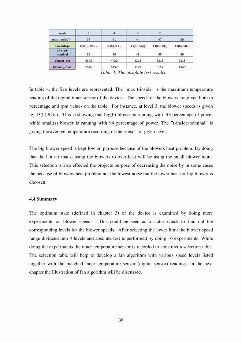
Table 4: The absolute test results.
In table 4, the five levels are represented. The ”max t-inside” is the maximum temperature
reading of the digital inner sensor of the device. The speeds of the blowers are given both in
percentage and rpm values on the table. For instance, at level 3, the blower speeds is given
by 43(b)-94(s). This is showing that big(b) blower is running with 43 percentage of power
while small(s) blower is running with 94 percentage of power. The ”t-inside-nominal” is
giving the average temperature recording of the sensor for given level.
The big blower speed is kept low on purpose because of the blowers heat problem. By doing
that the hot air that causing the blowers to over-heat will be using the small blower more.
This selection is also effected the projects purpose of decreasing the noise by in some cases
the because of blowers heat problem not the lowest noise but the lower heat for big blower is
choosen.
4.4 Summary
The optimum state (defined in chapter 3) of the device is examined by doing more
experiments on blower speeds. This could be seen as a status check to find out the
corresponding levels for the blower speeds. After selecting the lower limit the blower speed
range dividend into 4 levels and absolute test is performed by doing 16 experiments. While
doing the experiments the inner temperature sensor is recorded to construct a selection table.
The selection table will help to develop a fan algorithm with various speed levels listed
together with the matched inner temperature sensor (digital sensor) readings. In the next
chapter the illustration of fan algorithm will be discussed.
37
5 Fan Algorithm
5.1 Introduction
In chapter 2, we talked about the status check of the device and in chapter 3 we tried to find
the optimal state for the device with Taguchi method. Later, we continued with the absolute
tests to make a selection table for the fan algorithm in chapter 4. In this chapter a fan
algorithm schema will be given as taking a step forward on the project. This process will help
the device to adjust itself for various different environment conditions. The illustration will
be discussed in detail. [28]
5.2 Fan algorithm illustration
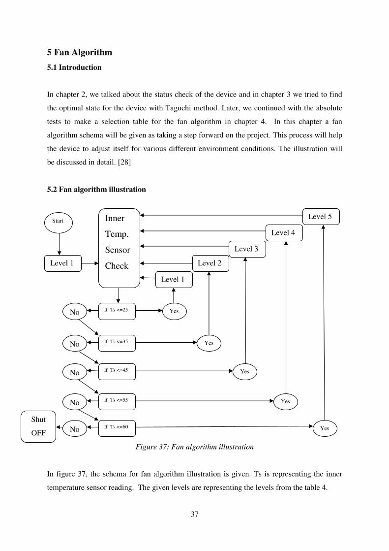
Figure 37: Fan algorithm illustration
In figure 37, the schema for fan algorithm illustration is given. Ts is representing the inner
temperature sensor reading. The given levels are representing the levels from the table 4.
Start Inner
Temp.
Sensor
Check
Level 4
Level 3
Level 5
Level 2
Level 1
If Ts <=25
If Ts <=35
If Ts <=45
If Ts <=55
If Ts <=60
Yes
Yes
Yes
Yes
Yes
No
No
No
No
No
Level 1
Shut
OFF

38
As the blowers start working at level 1(i.e. slow speeds) the Ts values are lower or equal to
the room temperature (24-25 degrees Celsius). As the Ts value increases the blower speeds
are increasing towards the level 5 gradually. It is important to note that the frequency of
checking the Ts value will determine the changes in the blower speeds levels. In addition,
how much time should be spending at each speed level should be defined. This is because as
working in a speed level the inner temperature is changing respectively.
5.3 Discussion on algorithm illustration
In this section we will try to address some scenarios for the fan algorithm illustration and
discuss those.
According to the illustration schema, if the device is at room temperature at the start then the
device will get hot as starting with low speed level (i.e. level 1) and the Ts value will
increase. As the Ts value increases the levels will increase also. Since Ts-maximum value is
44 (table 4) at level 3 the device speed will remain at level 3 at room temperature. If the Ts
temperature value is higher than 44 degrees Celsius, then the blowers will work at level 4.
This change from level 3 to level 4 will tent to decrease the Ts to 41 degrees Celsius at room
temperature. If the Ts values decrease at this point then the device could work at level 3
again and we will be back to where we started. This process will go iteratively, however we
could conclude that the device will work between level 3 and level 4 in room temperature.
In additional, if the Ts is higher than the room temperature the device will work at high levels
of speed. To determine the upper limit (environmental) that the device could handle in higher
temperatures the sensor readings should be examined. Here at this point we can not conclude
about the upper limit (environmental) of the device because of the fan and blowers heating
problem. However, we could add that if the blower and fan heating problem does not exist,
we could determine the upper limit. In that scenario, if we check the other sensor readings
(omitting fan and blower temperatures) and Ts-max is being equal to 37 as device is working
level 5, we could define the upper limit for the device as adding 24 to the room temperature.
The reason 24 degrees added to the room temperature is that the gap between the component
temperatures and their upper limit is on average 24 degrees. This will give 24+24=48 degrees
Celsius for the upper limit (environmental). If we examine the Ts value for the upper limit as
device being working at48 degrees Celsius then Ts value will be 37(for room temperature
39
highest Ts reading at level 5)+24(environment temperature-room temperature)= 61 and the
device will close itself as the limit is reached.
To sum up, illustrated fan algorithm if applied it will be working at room temperature and
temperatures close to room temperature +/-5 degrees Celsius. To define the upper limit for
environment temperature the fan and blower heat problem should be solved. Later on, the
device should be tested with the algorithm to record the temperatures of the critical
components in different scenarios. Later this data could be used for making the device adjust
itself for all environmental conditions. Further more, the component temperature values and
Ts values could be used to define the environment temperature.
5.4 Summary
Using the selection table (table 4) from chapter 4 the fan algorithm illustration is given.
Different scenarios about the illustration are examined. In addition, the upper limit for the
environmental temperature could not be defined due to fan and blower heating problem. Later
on, the device should be examined with the fan algorithm with various scenarios.
6 Conclusion and recommendations
6.1 Conclusion
The goal of the project was decreasing the noise of the device while keeping the temperature
values of the device within their limit temperatures. The whole process of trying to achieve
this goal is done in four parts. First, for decreasing the fan and blower speeds (which will
cause more heat in the system), the limit temperatures for the components are defined.
Second, an optimal state tried to be defined using DOE (Taguchi methods) for decreasing the
noise and temperature values. Third, further tests are applied to match inner sensor readings
with the blower speeds and room temperature taken as reference. Fourth, the fan algorithm
illustration is given and different scenarios are discussed. However, while doing the tests, a
problem (fan and blowers overheating problem) is found. Although, different methods tried
for solving the problem for the fan and blower over-heating problem could not solved. Thus,
the upper limit (environmental temperature) could not be defined. In addition, the selection
40
table in chapter 4 had to be dependent on the blower temperature values. Thus the noise
reduction for the device is effected as the blowers being the main source for the noise. In
future, fan and blower overheating problem should be solved in order to define upper limit of
the device and to decrease the noise.
6.2 Recommendations for future designs
There are two recommendations. First for solving the fan and blower heat problem and the
second is for applying the fan algorithm. First, to solve fan and blower heat problem should
be solved different scenarios could be applied. Such as:
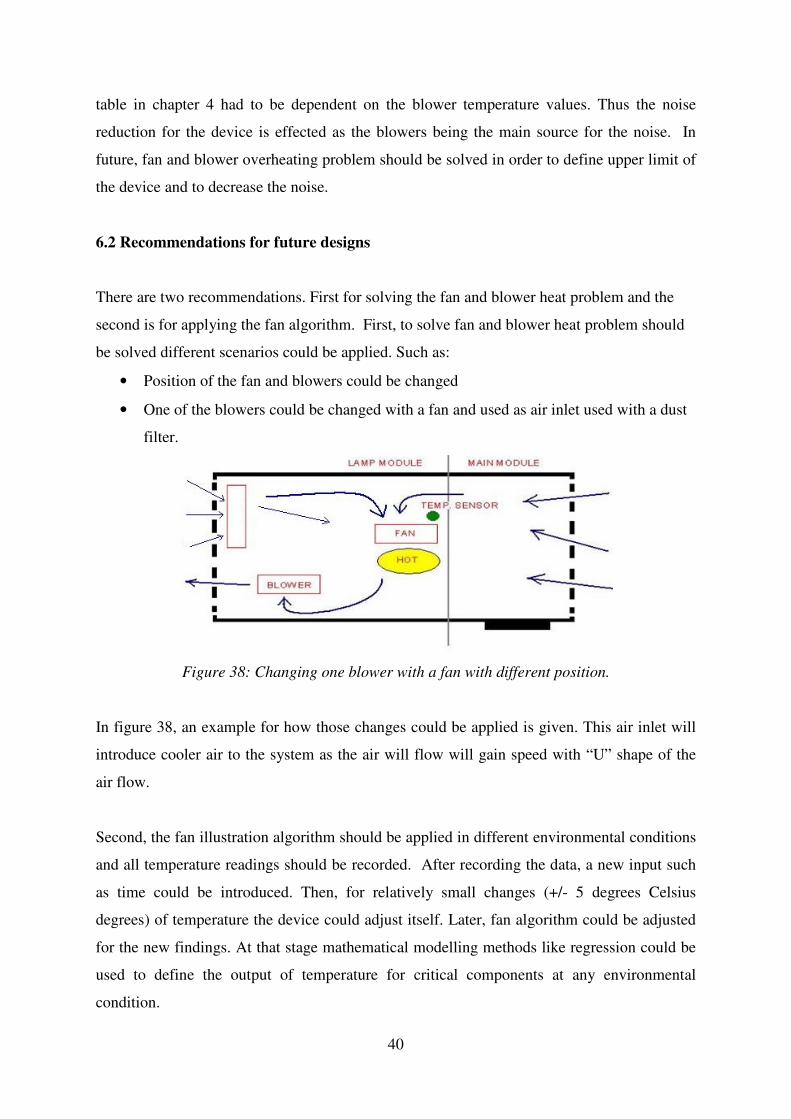
• Position of the fan and blowers could be changed
• One of the blowers could be changed with a fan and used as air inlet used with a dust
filter.
Figure 38: Changing one blower with a fan with different position.
In figure 38, an example for how those changes could be applied is given. This air inlet will
introduce cooler air to the system as the air will flow will gain speed with “U” shape of the
air flow.
Second, the fan illustration algorithm should be applied in different environmental conditions
and all temperature readings should be recorded. After recording the data, a new input such
as time could be introduced. Then, for relatively small changes (+/- 5 degrees Celsius
degrees) of temperature the device could adjust itself. Later, fan algorithm could be adjusted
for the new findings. At that stage mathematical modelling methods like regression could be
used to define the output of temperature for critical components at any environmental
condition.
41
REFERENCES
General information
[1] Optea AB website: www.optea.com
[2]Stroboscope and fan speed measurements website: www.bearblain.com/fan_speed_control.htm
[3] Agilent-Application Notes 290-Practical temperature measurements.
[4] Sound level meter website:en.wikipedia.org/wiki/Sound_level_meter
[5] Electus Distribution Reference Data Sheet: DECIBELS.PDF
[6] Agilent 34970A Data Acquisition / Switch Unit user guide.
[7] Minitab software website: www.minitab.com
Design of experiments
[8] Mathews P.,Design of Experiments with Minitab,(2005),(P:93),ASQ
[9] Awell run design of experiments website: www.qualitydigest.com/june01/html/sixteen.html
[10]Doe with taguchi method website:
controls.engin.umich.edu/wiki/index.php/Design_of_experiments_via_taguchi_methods:_orthogonal_arrays
[11] Anthony, J, Capon N.,Teaching Experimental Design Techniques to Industrial Engineers ,(1998)
[12] Mason, PW , Prevey PS, Iterative taguchi analyses: optimising the austenite content and hardness in 52100
steel, Journal of materials engineering and performance, Vol:10, Num:1. 14-21, Springer.
[13] Montogmery, D, Design and analysis of experiments,(2001) (P:17)(John Wiley, Sons).
[14] Sang Gil P, Analysis of HVAC systems sound quality using design of experiments,. Journal of Mechanical
Science and Technology, Vol: 23, Springer.
[15] Touch temperature design requirements website: http://msis.jsc.nasa.gov/sections/section06.htm
[16] H. -W. Chi , C. L. Bloebaum, Mixed variable optimization using Taguchi's orthogonal arrays, Structural
and Multidisciplinary Optimization ,Vol: 12, Num: 2-3, 147-152, Springer
Inner documents-Optea AB
[17] 22-DigiMap2-00001-05
[18] 22-Digimap2-00005-03
[19] 22-DigiMap2-00013-01
[20] 22-DigiMap2-00009-02
[21] 22-DigiMap2-00009-03
[22] 22-DigiMap2-00009-04
[23] 22-DigiMap2-00012-01
[24] 22-DigiMap2-00010-01
[25] 22-DigiMap2-00015-01
[26] 22-DigiMap2-00016-01
[27] 22-DigiMap2-00017-01
[28] 22-DigiMap2-00018-01

42
APPENDIXES
APPENDIX A: Stroboscope readings
Measured rpm values with stroboscope with noise measurements.
small
blower dbA
big
blower dbA fan dbA approximate
voltage RPM RPM RPM PERCENTAGE
12 7546 73 5375 70 7286 66 100
11.5 7357 72.5 5243 70 7054 65 97
11 7129 72.5 5103 69 6818 65 94
10.5 6906 71.5 4946 68 6596 64.5 91
10 6658 71 4798 67 6355 63 88
9.5 6407 70.5 4604 66 6051 62 84
9 6157 70 4430 66 5843 61 80
8.5 5868 69 4230 64 5537 59 77
8 5580 68 4018 63 5259 58 74
7.5 5251 67 3789 61 4955 57 69
7 4946 65 3529 59 4585 55 64
6.5 4580 64 3243 57 4240 53 60
6 4203 62 2959 55 3877 51 55
5.5 3851 59 2674 53 3475 50 50
5 3415 55 2215 50 3035 50 43
4.5 2983 52 1849 48 2708 49 40
At 7 volts using 64 percentage of the power, the device closed itself after 15min. the dbA
measures are taken 3cm away from the fan and blowers.
15002000250030003500400045005000550060006500700075008000
12 11 10 9 8 7 6 5
small_blower
big_blower
fan
43
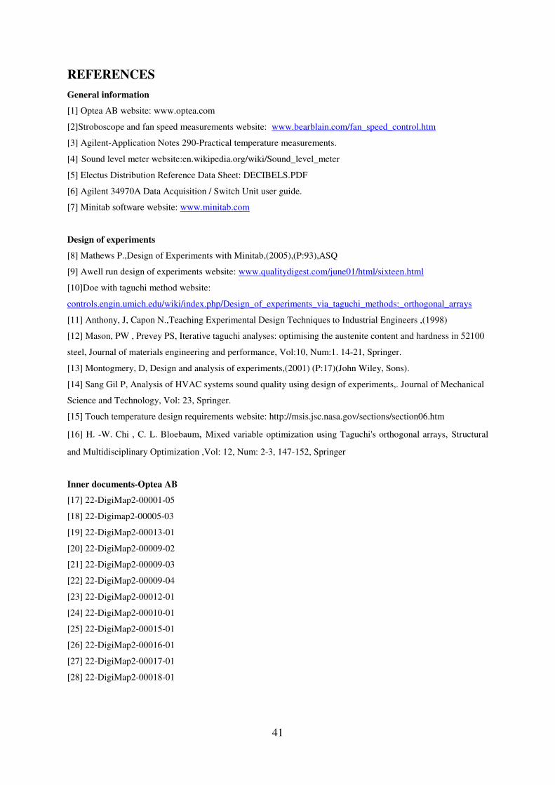
APPENDIX B: Sound level meter
Relative to human hearing the sound pressure levels.
SOUND PRESSURE LEVELS IN DB
(RELATIVE TO O.2 nanoBar RMS at 1kHz)
140dB Large industrial siren
130dB Threshold of feeling or pain
120dB aircraft engine
110dB Rock band performance
100dB Close to loud car or truck horn
90dB Human hearing at risk
80dB Orchestra
70dB Inside factory
65dB Typical office conversation
45dB Inside home residence
30dB Soft or background music
20dB Quiet whisper
0dB Threshold of hearing
44
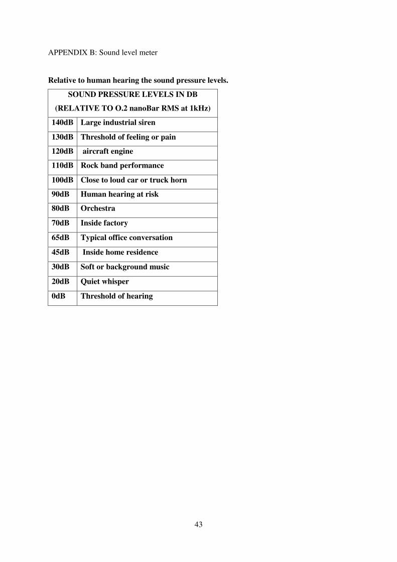
APPENDIX C: Thermocouples are connected to data logger
User guide of Agilent34970A could be examined for further details.
APPENDIX D: K type thermocouple
Thermocouple measurements for the temperatures are between +/- 1.5 Degrees Celsius
tolerance. Type K (chromel–alumel) is the most common general purpose thermocouple.
For additional detail on range and tolerance see: http://en.wikipedia.org/wiki/Thermocouples

45
APPENDIX E:
Digital temperature sensor, with I2C interface.
Digital sensor with I2C interface is giving the sensor readings in hexadecimal numbers so
conversion is needed to decimal numbers for reading the temperature values. The calculation
below is given could be used in an excel file. A10 is representing any given cell that the data
is given.
Temperature calculation=0.0625*(HEX2DEC(A10))/16
Example:
1800 = 24 Degrees celcius.
APPENDIX F
Orthogonal array selector represented for small size of parameter (inputs).
Number of levels Number of inputs
2 3 4 5
2 L4 L4 L8 L8
3 L9 L9 L9 L18
4 L’16 L’16 L’16 L’16
5 L25 L25 L25 L25
Orthogonal array selection example:
L9 is selected for 3 level and 4 input from the array selector as represented in gray boxes
above on array selection matrix.
L9 Orthogonal Array
Experiments Input1 Input2 Input3 Input4
1 1 1 1 1
2 1 2 2 2
3 1 3 3 3
4 2 1 2 3
5 2 2 3 1
6 2 3 1 2
7 3 1 3 2
8 3 2 1 3
9 3 3 2 1
46
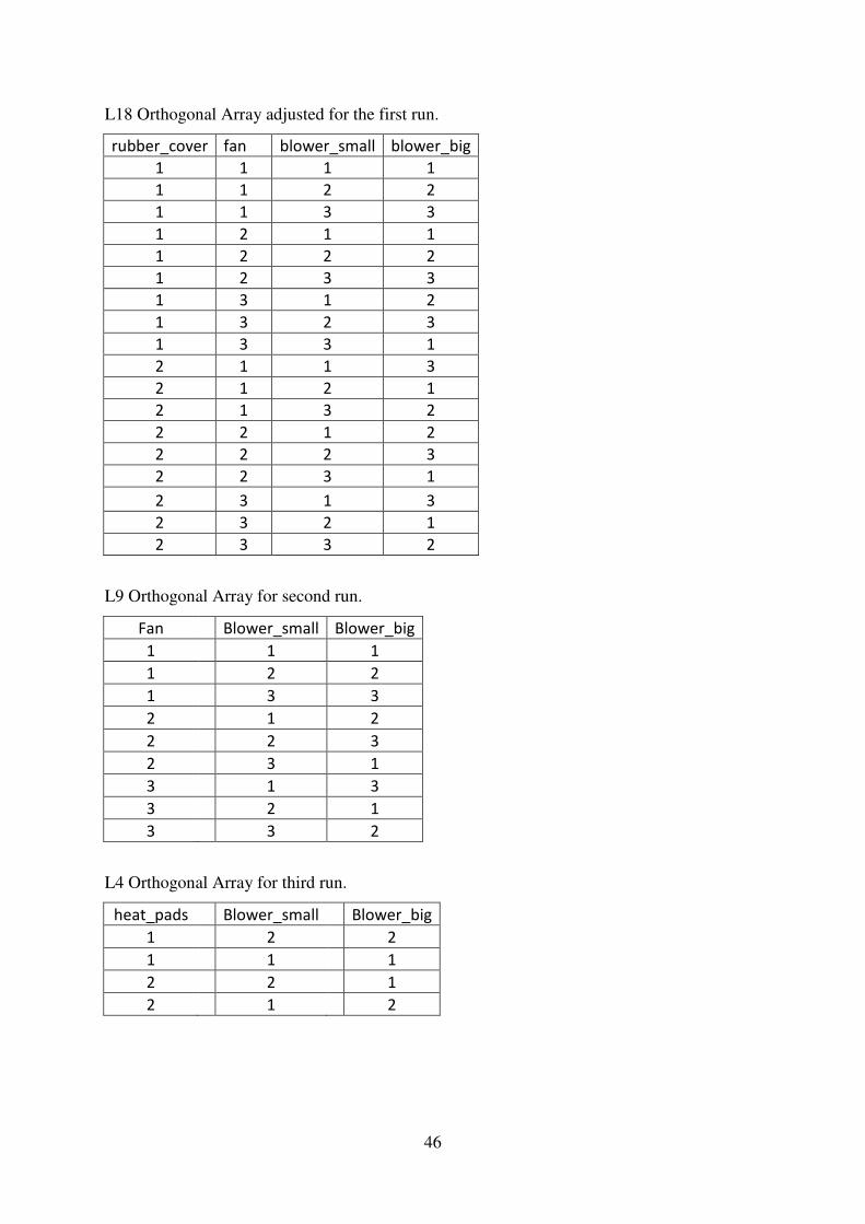
L18 Orthogonal Array adjusted for the first run.
rubber_cover fan blower_small blower_big
1 1 1 1
1 1 2 2
1 1 3 3
1 2 1 1
1 2 2 2
1 2 3 3
1 3 1 2
1 3 2 3
1 3 3 1
2 1 1 3
2 1 2 1
2 1 3 2
2 2 1 2
2 2 2 3
2 2 3 1
2 3 1 3
2 3 2 1
2 3 3 2
L9 Orthogonal Array for second run.
Fan Blower_small Blower_big
1 1 1
1 2 2
1 3 3
2 1 2
2 2 3
2 3 1
3 1 3
3 2 1
3 3 2
L4 Orthogonal Array for third run.
heat_pads Blower_small Blower_big
1 2 2
1 1 1
2 2 1
2 1 2
47
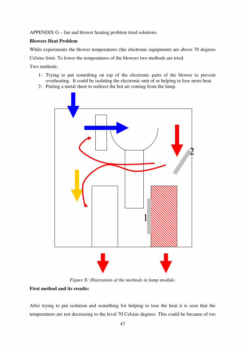
APPENDIX G – fan and blower heating problem tried solutions.
Blowers Heat Problem
While experiments the blower temperatures (the electronic equipment) are above 70 degrees
Celsius limit. To lower the temperatures of the blowers two methods are tried.
Two methods:
1- Trying to put something on top of the electronic parts of the blower to prevent
overheating. It could be isolating the electronic unit of or helping to lose more heat.
2- Putting a metal sheet to redirect the hot air coming from the lamp.
Figure X: Illustration of the methods in lamp module.
First method and its results:
After trying to put isolation and something for helping to lose the heat it is seen that the
temperatures are not decreasing to the level 70 Celsius degrees. This could be because of too
1
2

little space that putting something thick would cause touching the lamp and putting
something little is not helping the air flow in that part of the lamp module. The main effect of
this will be discussed in the conclusion.
Second method and its results:
Trying to change the direction of the hot air with various size metal sheets placed before the
big blower. After several attempts while the fan and blowers are working at full speed the
data is recorded. It is seen that putting metal sheet to change the di
helping to decrease the temperature of the blowers to desired 70 degrees Celsius level.
Conclusion
The both of the methods could not decrease the blower temperatures to desired 70 degrees
Celsius. Since the hot air coming f
blowers are getting hot as being the only air out part of the system.
Try out pictures for second method with two different sizes of metal sheets.
48
little space that putting something thick would cause touching the lamp and putting
ttle is not helping the air flow in that part of the lamp module. The main effect of
this will be discussed in the conclusion.
Second method and its results:
Trying to change the direction of the hot air with various size metal sheets placed before the
big blower. After several attempts while the fan and blowers are working at full speed the
data is recorded. It is seen that putting metal sheet to change the direction of the hot air is not
helping to decrease the temperature of the blowers to desired 70 degrees Celsius level.
The both of the methods could not decrease the blower temperatures to desired 70 degrees
Celsius. Since the hot air coming from the lamp is the main reason for overheating, the
blowers are getting hot as being the only air out part of the system.
s for second method with two different sizes of metal sheets.
little space that putting something thick would cause touching the lamp and putting
ttle is not helping the air flow in that part of the lamp module. The main effect of
Trying to change the direction of the hot air with various size metal sheets placed before the
big blower. After several attempts while the fan and blowers are working at full speed the
rection of the hot air is not
helping to decrease the temperature of the blowers to desired 70 degrees Celsius level.
The both of the methods could not decrease the blower temperatures to desired 70 degrees
rom the lamp is the main reason for overheating, the
s for second method with two different sizes of metal sheets.
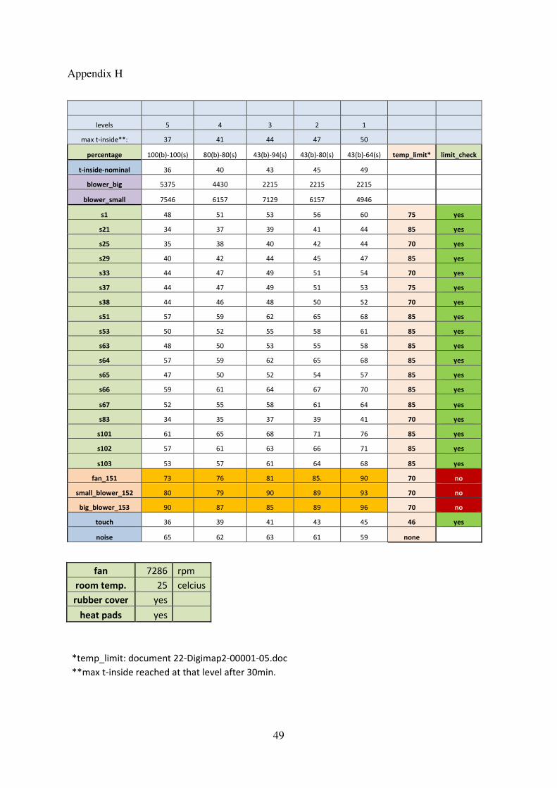
49
Appendix H
levels 5 4 3 2 1
max t-inside**: 37 41 44 47 50
percentage 100(b)-100(s) 80(b)-80(s) 43(b)-94(s) 43(b)-80(s) 43(b)-64(s) temp_limit* limit_check
t-inside-nominal 36 40 43 45 49
blower_big 5375 4430 2215 2215 2215
blower_small 7546 6157 7129 6157 4946
s1 48 51 53 56 60 75 yes
s21 34 37 39 41 44 85 yes
s25 35 38 40 42 44 70 yes
s29 40 42 44 45 47 85 yes
s33 44 47 49 51 54 70 yes
s37 44 47 49 51 53 75 yes
s38 44 46 48 50 52 70 yes
s51 57 59 62 65 68 85 yes
s53 50 52 55 58 61 85 yes
s63 48 50 53 55 58 85 yes
s64 57 59 62 65 68 85 yes
s65 47 50 52 54 57 85 yes
s66 59 61 64 67 70 85 yes
s67 52 55 58 61 64 85 yes
s83 34 35 37 39 41 70 yes
s101 61 65 68 71 76 85 yes
s102 57 61 63 66 71 85 yes
s103 53 57 61 64 68 85 yes
fan_151 73 76 81 85. 90 70 no
small_blower_152 80 79 90 89 93 70 no
big_blower_153 90 87 85 89 96 70 no
touch 36 39 41 43 45 46 yes
noise 65 62 63 61 59 none
fan 7286 rpm
room temp. 25 celcius
rubber cover yes
heat pads yes
*temp_limit: document 22-Digimap2-00001-05.doc
**max t-inside reached at that level after 30min.