École doctorale de mathématiques Hadamard

These de doctoratSpécialité : Mathématiques

présentée par

Hsueh-Yung LIN

Invariants symplectiques et zéro-cycles dans lesvariétés hyper-kählériennes

dirigée par Claire VOISIN

Soutenue le XXX devant le jury composé de :

M. Sébastien BOUCKSOM École Polytechnique examinateurM. Olivier DEBARRE École Normale Supérieure examinateurM. Kieran O’GRADY Università di Roma rapporteurM. Gianluca PACIENZA Université de Strasbourg rapporteurM. Nicolas PERRIN Université de Versailles Saint-Quentin-en-Yvelines examinateurMme Claire VOISIN Université Paris VI directrice de thèse

2

Thèse préparée auCentre de Mathématiques LaurentSchwartzUMR CNRS 7640École Polytechnique91 128 Palaiseau CEDEX

Table des matières

Introduction 5

0.1 Géométrie symplectique et géométrie kählérienne . . . . . . . . . . . . . . . . . . . 5

0.2 Variétés projectives complexes et leurs cycles algébriques . . . . . . . . . . . . . . . 12

0.3 Variétés hyper-kählériennes . . . . . . . . . . . . . . . . . . . . . . . . . . . . . . . . 16

1 Canonical bundle and symplectic geometry 21

1.1 Introduction . . . . . . . . . . . . . . . . . . . . . . . . . . . . . . . . . . . . . . . . . 21

1.2 Classification of non-splitting families of rational curves . . . . . . . . . . . . . . . 23

1.3 Gromov-Witten invariants . . . . . . . . . . . . . . . . . . . . . . . . . . . . . . . . . 24

1.4 Non-nef canonical bundle and symplectic geometry . . . . . . . . . . . . . . . . . . 25

2 Singularities of curves and Beauville-Voisin zero-cycle 29

2.1 Introduction . . . . . . . . . . . . . . . . . . . . . . . . . . . . . . . . . . . . . . . . . 29

2.2 Universal deformation space of morphisms from elliptic curves to a fixed K3 surface 31

2.3 Cusp locus and c2(S) . . . . . . . . . . . . . . . . . . . . . . . . . . . . . . . . . . . . 33

2.4 Double point locus . . . . . . . . . . . . . . . . . . . . . . . . . . . . . . . . . . . . . 35

2.5 Proof of Theorem 2.3 . . . . . . . . . . . . . . . . . . . . . . . . . . . . . . . . . . . . 38

3 Rational maps from K3[n] 45

3.1 Introduction . . . . . . . . . . . . . . . . . . . . . . . . . . . . . . . . . . . . . . . . . 45

3.2 Remarks on rationally connected varieties . . . . . . . . . . . . . . . . . . . . . . . . 47

3.3 Proof of Theorem 3.1 . . . . . . . . . . . . . . . . . . . . . . . . . . . . . . . . . . . . 48

3.4 Triviality of symplectic involution actions on CH0(S) . . . . . . . . . . . . . . . . . . 49

4 Miscellaneous properties of Lagrangian fibrations 53

4.1 Introduction . . . . . . . . . . . . . . . . . . . . . . . . . . . . . . . . . . . . . . . . . 53

4.2 Hyper-Kähler manifolds and Lagrangian fibrations . . . . . . . . . . . . . . . . . . 55

4.3 Base variety of rationally fibered Calabi-Yau manifolds . . . . . . . . . . . . . . . . 56

4.4 A VHS viewpoint of Lagrangian fibrations . . . . . . . . . . . . . . . . . . . . . . . 57

4.5 Cubics . . . . . . . . . . . . . . . . . . . . . . . . . . . . . . . . . . . . . . . . . . . . 59

4.6 Transcendental second Betti number and isotrivial Lagrangian fibrations . . . . . . 61

5 Lagrangian constant cycle subvarieties in Lagrangian fibrations 65

5.1 Introduction . . . . . . . . . . . . . . . . . . . . . . . . . . . . . . . . . . . . . . . . . 65

5.2 Construction of constant cycles subvarieties on Lagrangian fibrations . . . . . . . . 67

4 Table des matieres

6 Chow group of 0-cycles of a generalized Kummer variety 716.1 Introduction . . . . . . . . . . . . . . . . . . . . . . . . . . . . . . . . . . . . . . . . . 716.2 Constructing Ci-subvarieties in generalized Kummer varieties . . . . . . . . . . . . 736.3 The support of SiCH0(X) . . . . . . . . . . . . . . . . . . . . . . . . . . . . . . . . . . 766.4 The induced Beauville decomposition on generalized Kummer varieties . . . . . . 846.5 The rational orbit filtration and the induced Beauville decomposition coincide . . . 86

Bibliographie 91

Introduction

Cette thèse vise à comprendre la géométrie d’une variété donnée via l’étude de certainsinvariants associés à des sous-variétés (ou cycles) des variétés symplectiques, kählériennes etalgébriques complexes. Elle se compose de trois parties. Le Chapitre 1 seul forme une premièrepartie indépendante du reste de cette thèse, concernant l’aspect symplectique des variétés käh-lériennes. Nous y démontrons l’invariance symplectique de l’effectivité numérique du fibré endroites canonique d’une variété kählérienne compacte de dimension trois, résultat paru auxMathematical Research Letters [Lin14a]. Les Chapitres 2 et 3 forment une deuxième partie dethèse, qui débute l’étude des zéro-cycles par le cas des surfaces K3 algébriques, regroupant deuxarticles publiés respectivement dans le journal Manuscripta Mathematica [Lin15] et le Bollettinodell’Unione Matematica Italiana [Lin14b]. Dans la dernière partie du texte (Chapitre 4 à 6), nousy abordons l’étude des zéro-cycles sur une variété hyperkählérienne projective, l’analogue endimension supérieure des surfaces K3. Nous nous concentrerons en particulier sur les variétéshyperkählériennes polarisées admettant une fibration lagrangienne et les variétés de Kummergénéralisées.

Dans cette introduction, nous allons présenter les contextes généraux dans lesquels cette thèses’inscrit et les théories générales dont nous nous servirons dans cette thèse.

0.1 Géométrie symplectique et géométrie kählérienne

Le but de cette section est de présenter la géométrie kählérienne et quelques invariants attachésaux variétés kählériennes avec l’accent mis d’une part, sur le programme des modèles minimaux etd’autre part, sur l’aspect symplectique de ces invariants afin de motiver et énoncer le Théorème 0.13que nous obtenons dans le Chapitre 1.

0.1.1 Variétés kählériennes

Soit (X, J) une variété complexe munie d’une métrique hermitienne h sur le fibré tangentcomplexifié TX,C. Si la structure complexe J ∈ End(TX,R) est plate pour la connexion de Levi-Civita∇ de la métrique riemannienne 1 :=<(h), on dit que h est une métrique kählérienne. Cette dernièrecondition est équivalente à la fermeture de la 2-forme symplectique ω := −=(h) et si c’est le cas, Xest appelée une variété kählérienne et ω sa forme de Kähler. Une forme de Kähler est en particulierune forme symplectique sur X, et la notion de kählérianité évoque une compatibilité naturelleentre les structures complexe, riemannienne, et symplectique de X. Par principe d’holonomie, onvoit aussi que h est kählérienne si, et seulement si, le groupe d’holonomie Hol(1) est contenu dansun sous-groupe conjugué à U(n) où n = dimC X ; nous y reviendrons dans le paragraphe 0.3.

Des exemples de variétés kählériennes sont fournis par les variétés projectifs complexes muniesde leur métrique de Fubini-Study. Si X ⊂ PN est une variété projective, la forme de Kählerω associée

6 Introduction

à sa métrique de Fubini-Study représente la première classe de Chern de la restriction sur X du dualde la fibré en droite tautologique sur PN, donc [ω] ∈ H2(X,Z). Réciproquement, la non-existenced’une classe de Kähler entière est la seule obstruction à plonger holomorphiquement une variétécompacte kählérienne dans un espace projectif [Kod54].

Différentes notions de positivité et dualité des cônes positifs

Soit X une variété complexe. L’image de l’application première classe de Chern c1 : Pic(X) →H2(X,Z) dans H2(X,Z) est appelée groupe de Néron-Severi de X et sera notée NS(X). Si de plus X estcompacte et kählérienne, on a

NS(X) =(H2(X,Z)/tors

)∩H1,1(X). (1)

Ci-dessous nous rappelons la définition des différents cônes positifs, d’abord dans le groupe deNéron-Severi réel d’une variété complexe projective (lisse), puis leur généralisation dans le caskählérien.

Pour une variété projective X, on définit le cône ample Amp(X) comme le cône (ouvert) convexedans NSR(X) := NS(X) ⊗ R engendré par les classes de diviseurs amples. Sa fermeture Nef(X) :=Amp(X) ⊂ NSR(X) est appelée le cône nef de X. On définit aussi le cône pseudo-effectif Psef(X)comme l’adhérence dans NSR(X) du cône convexe engendré par les classes de diviseurs effectifs.Les diviseurs dont la classe se situe à l’intérieur de Psef(X) sont appelés les diviseurs gros.

Dans le cas kählérien compacte, les cônes de positivité qui généralisent ceux ci-dessus sontdéfinis dans H1,1(X)R := H2(X,R) ∩H1,1(X) (ne serait-ce que parce que le groupe de Néron-Severiest réduit à 0 si X n’est pas projective). L’analogue kählérien du cône ample est le cône de Kähler,qui est le cône (ouvert) convexe K dans H1,1(X)R engendré par les classes de formes de Kählerde X. En effet si X est projective, d’une part le cône ample (resp. Nef(X)) est la trace du cône deKähler (resp. K [Dem92]) dans NSR(X), d’autre part de même que Nef(X) est le cône dual par leproduit d’intersection de l’adhérence du cône engendré par les classes de 1-cycles effectifs dans

N1(X)R :=(Hn−1,n−1(X) ∩H2n−2(X,Q)

)⊗ R (2)

d’après le critère de Kleiman, de même K est le dual du cône convexe dans Hn−1,n−1R (X) :=

Hn−1,n−1(X) ∩ H2n−2(X,R) engendré par les classes de courants réels positifs de type (n − 1,n −1) [DP04].

L’analogue kählérien du cône pseudo-effectif est le cône fermé convexe E engendré par lesclasses de courants réels positifs de type (1, 1), qui vérifie E ∩ NSR(X) = Psef(X) dans le casprojectif [Dem92]. Conjecturalement E est dual du cône convexe fermé M engendré par les classesmobiles dans Hn−1,n−1

R (X). Dans le cas projectif, M ∩ N1(X)R coïncide avec le cône fermé convexeengendré par les classes de courbes mobiles, qui sont par définition les courbes dont la déformation(algébrique) recouvre X. De plus,

Théorème 0.1 (Boucksom-Demailly-Paun-Peternell [BDPP13]). Le cône pseudo-effectif d’une variétécomplexe projective lisse X est le dual de M ∩N1(X)R.

Voici un corollaire important de du Théorème 0.1.

Corollaire 0.2 (Boucksom-Demailly-Paun-Peternell [BDPP13]). Une variété compacte projective Xest uniréglée si et seulement si KX est pseudo-effective.

0.1. Geometrie symplectique et geometrie kahlerienne 7

Le même énoncé dans le cas kählérien reste conjectural (à comparer avec la Conjecture 0.6).Ici, KX := ∧dim XΩ1

X est le fibré en droite canonique de X. Une variété compacte kählérienne est diteuniréglée si elle est couverte par des images non-constantes de P1.

0.1.2 Classification des variétés compactes kählériennes

Programme des modèles minimaux

Dans ce qui suit, nous esquissons le programme des modèles minimaux dû à Mori qui vise àchercher la variété projective la plus simple dans chaque classe birationnelle. Nous renvoyonsà [Deb01] et [KM98] pour les détails et des généralisations.

Soient X une variété projective lisse complexe et KX son diviseur canonique (bien défini àéquivalence linéaire près). Le cône de courbes NE(X) est défini comme le cône fermé convexeengendré dans l’espace des 1-cycles modulo équivalence numérique par les classes de courbesdans X. C’est un cône fortement convexe d’après le critère de Kleiman. Pour tout R-diviseur L,posons

NE(X)L≥0 :=α ∈ NE(X) | α · L ≥ 0

. (3)

Théorème 0.3 (Mori). Il existe une famille dénombrable de courbes rationnelles (Ci ⊂ X)i∈I avec KX ·Ci < 0telle que R≥0[Ci] soit un rayon extrémal dans NE(X) et que

NE(X) = NE(X)KX≥0 +∑i∈I

R≥0[Ci]. (4)

De plus, pour tout R-diviseur ample H, il existe une partie finie I′ ⊂ I telle que

NE(X) = NE(X)KX+H≥0 +∑i∈I′

R≥0[Ci]. (5)

Les rayons extrémaux R≥0[Ci] de NE(X)KX<0 sont appelés rayons extrémaux de Mori. Kawamatadémontra que pour chaque rayon extrémal de Mori R≥0[Ci], il existe une variété normale Y et unmorphisme surjectif X→ Y qui contracte toutes les courbes dont la classe appartient à R≥0[Ci]. Leprogramme des modèles minimaux consiste à chercher des modifications birationnelles contractantces courbes extrémales tout en garantissant que les singularités de Y sont modérées jusqu’à obtenirune variété Xm dont le fibré en droite canonique est nef si κ(X) ≥ 0 où κ(X) désigne la dimensionde Kodaira de X, ou un espace fibré de Mori sinon. L’existence de telles modifications birationnellesest connue grâce à [BCHM10], tandis que la terminaison de ce programme reste conjecturale endimension ≥ 5 (cf. [KMM87] pour la terminaison en dimension ≤ 4).

Un espace fibré de Mori est un morphisme projectif surjectif dont la fibre générale est unevariété de Fano. L’existence de l’espace fibré de Mori pour une variété uniréglée suggérée par leprogramme des modèles minimaux est à comparer avec le théorème suivant.

Théorème 0.4 ([KMM92b, Cam81]). Soit X une variété compacte kählérienne lisse. Il existe une uniqueapplication (à bi-méromorphismes près) presque holomorphe f : Xd Y telle que

i) une fibre générale de f est rationnellement connexe ;

ii) pour tout point général y ∈ Y et toute courbe rationnelle C ⊂ X passant par f−1(y), on a C ⊂ f−1(y).

Ici, une variété X est rationnellement connexe si deux points généraux dans X sont connectéspar une chaîne de courbes rationnelles. Les variétés de Fano sont des exemples (non évidents) devariétés rationnellement connexes [KMM92a, Cam92]. On appelle l’application f : X d Y dans

8 Introduction

le Théorème 0.4 le quotient rationnellement connexe maximal de X. La base d’un tel quotient n’estjamais uniréglée grâce au théorème de Graber, Harris et Starr [GHS03] :

Théorème 0.5 (Graber-Harris-Starr). Soit f : X→ Y un morphisme propre d’une variété complexe surune courbe lisse. Si la fibre générale de f est rationnellement connexe, alors f a une section.

Il est également possible d’étendre le programme de modèles minimaux au cas kählérien. Endimension 3, ce projet fut mené et achevé par Campana, Höring et Peternell ; nous renvoyonsà [HP13, CHP14] et aux références qui s’y trouvent.

Variétés de dimension de Kodaira −∞ ou 0

Rappelons que si X est une courbe complexe compacte de genre 1 := dimC H0(X,Ω1X), par le

théorème d’uniformisation de Poincaré, X porte une métrique à courbure constante K et les casK > 0, K = 0 et K < 0 correspondent respectivement aux situations 1 = 0 (sphère de Riemann),1 = 1 (courbe elliptique) et 1 ≥ 2. Si κ(X) désigne la dimension de Kodaira, cette trichotomiecorrespond aussi à κ(X) < 0, κ(X) = 0 et κ(X) > 0 respectivement.

Dans le cas général, voici la description conjecturale des variétés de dimension de Kodaira −∞.

Conjecture 0.6. Soit X une variété compacte kählérienne. Les assertions suivantes sont équivalentes :

i) κ(X) < 0 ;

ii) KX n’est pas pseudo-effectif ;

iii) X est uniréglée.

L’implication iii) =⇒ ii) =⇒ i) est facile. La Conjecture 0.6 est connue en dimension ≤ 3,d’abord dans le cas projectif [Mor88], puis dans le cas général [Bru06, CHP14]. Lorsque X estprojective, on a vu l’équivalence entre ii) et iii) (cf. Théorème 0.1).

Quant aux variétés minimales de dimension de Kodaira 0, les variétés compactes kählériennesdont la première classe de Chern est triviale sont des exemples de telles variétés. La réciproqueserait une conséquence de la conjecture suivante :

Conjecture 0.7 (Conjecture d’abondance). Soit X une variété compacte kählérienne dont le fibré endroite canonique KX est nef (i.e. la classe c1(KX) appartient à l’adhérence du cône de Kähler de X). Il existem ∈ Z>0 tel que mKX est sans lieu de base.

Comme la Conjecture 0.6, la Conjecture 0.7 est connue en dimension 3, d’abord dans le casprojectif [Mor88], puis le cas général [CHP14]. Si X est minimale et κ(X) = 0, la conjectured’abondance implique qu’il existe m > 0 tel que le système linéaire |mKX| définit un morphismede X vers un point et en particulier, KX est de torsion. D’où c1(X) = 0. Nous reviendrons sur cesvariétés au paragraphe 0.3.

0.1.3 Variétés symplectiques et théorie de Gromov-Witten

Par définition, une variété symplectique est une variété différentielle X munie d’une 2-formedifférentielleω fermée et partout non-dégénérée. Nous renvoyons à [Arn89] pour une présentationde son origine riche provenant de la mécanique classique. D’après le théorème de Darboux, laprésence ou non d’une forme symplectique n’influence pas la géométrie locale de X. En revanche,la non-dégénérescence de la forme symplectique ω impose déjà des contraintes topologiquesévidentes sur X : une variété symplectique est toujours de dimension paire 2n et orientable. Si deplus X est compacte, il s’ensuit que ses groupes de cohomologie singulière de codimension pairene s’annulent pas.

0.1. Geometrie symplectique et geometrie kahlerienne 9

Souplesse et rigidité de la structure symplectique

Ci-dessous nous allons illustrer par des exemples la souplesse par rapport à la structurekählérienne et la rigidité par rapport à la structure différentielle de la structure symplectique.

La souplesse de la structure symplectique par rapport à la structure kählérienne se voit déjàau niveau local d’après le théorème de Darboux. Au niveau global, topologiquement tout groupede présentation finie est réalisable comme groupe fondamental d’une variété symplectique dedimension paire fixée [Gom95], mais il existe de sévères contraintes sur le groupe fondamentald’une variété kählérienne (voir [Bur11]). Entre différentes variétés symplectiques nous étudionsles morphismes symplectiques, qui, par définition est un morphisme différentiable f : X → Y entredeux variétés symplectiques (X, ω) et (Y, ω′) tel que f ∗ω′ = ω. Le groupe des automorphismesholomorphes d’une variété kählérienne (préservant la forme kählérienne ou non) est de dimensionfinie, tandis que le groupe des automorphismes symplectiques est un groupe de Lie de dimensioninfinie. Enfin, en théorie de Gromov-Witten, comme nous le verrons plus tard l’espace de modulede certaines courbes pseudo-holomorphes M est de dimension attendue d pour une structurepresque complexe générale compatible avec la forme symplectique, mais il peut ne pas exister dedéformation kählérienne pour laquelle M est de dimension d.

La rigidité de la structure symplectique est plus subtile que sa souplesse. Si dim X = dim Y,il est évident qu’un morphisme symplectique préserve en particulier le volume défini par leurforme symplectique. Un tel morphisme est en fait bien plus rigide, comme le montre le théorèmesuivant :

Théorème 0.8 (Théorème de non-écrasement de Gromov [Gro85]). Munis de leur forme symplectiquestandard, il n’existe pas de morphisme symplectique d’une boule euclidienne B ⊂ R2n de rayon R versR2n−2

×D où D ⊂ R2 est un disque euclidien de rayon r < R.

L’idée de Gromov derrière les résultats de rigidité de la structure symplectique tels quele théorème de non-écrasement, est basée sur la présence des courbes pseudo-holomorphes, quigénéralise la notion des courbes holomorphes dans les variétés complexes que nous rappelonsdans les paragraphes suivants.

Structures presque complexe d’une variété symplectique

Étant donnée une variété complexe X, sur chaque carte locale Ui, il existe un endomorphismeJi du fibré tangent TUi,R tel que J J = −IdTUi ,R

, hérité de la structure complexe standard de C,. CesJi se recollent en un champs de tenseurs J ∈ Γ(X,End(TX,R)) de classe C∞ tel que

J J = −IdTX,R , (6)

que l’on appelle la structure complexe de X. En général, un champs de tenseurs J ∈ Γ(X,End(TX,R))sur une variété différentielle X qui satisfait la condition (6) est appelée une structure presque complexede X. De façon équivalente, il revient au même de se donner une décomposition C∞ du complexifiéde TX,R en la somme de deux sous-fibrés conjugués complexes l’un de l’autre

TX,C = T1,0X ⊕ T0,1

X (7)

10 Introduction

où T1,0X (resp. T0,1

X ) est le sous-fibré propre de J de valeur propre i (resp. −i). Par suite, en chaquepoint p ∈ X il existe des coordonnées locales (x1, . . . , xn, y1, . . . , yn) telles que pour tout 1 ≤ j ≤ n,

J∂

∂x j =∂

∂y j et J∂

∂y j = −∂

∂x j . (8)

Lorsque J provient d’une structure complexe, il est évident que sur chaque carte locale Ui, on peuttrouver des coordonnées locales (x1, . . . , xn, y1, . . . , yn) telles que (8) soit vérifiée pour tout p ∈ Ui.Une structure presque complexe s’intègre en une structure complexe si, et seulement si, elle vérifiele critère d’intégrabilité de Newlander-Nirenberg [NN57] :

[T0,1X ,T0,1

X ] ⊂ T0,1X . (9)

Sur une variété symplectique (X, ω), on dit qu’une structure presque complexe J est ω-contrôléesi ω(u, Ju) > 0 pour tous vecteurs tangents non-nuls u. Pour une variété symplectique (X, ω),Gromov montra que les structures presque complexes ω-contrôlées (resp. ω-compatibles) formentun sous-ensemble non-vide et contractile dans End(TX). Une application différentiable entre deuxvariétés presque complexes f : (X, J)→ (Y, J′) est dite pseudo-holomorphe si l’on a la commutationd f J = J′ d f . Lorsque X et Y sont des variétés complexes, cette définition coïncide avec celled’une application holomorphe.

Invariants de Gromov-Witten

La principale référence de ce paragraphe est [MS12].

On appelle courbe pseudo-holomorphe dans (X, J) l’image d’une application pseudo-holomorphef : Σ→ X où S est une surface de Riemann. En général, l’existence locale de sous-variétés pseudo-holomorphes dépend de l’intégrabilité de la structure presque complexe J, mais celle de courbespseudo-holomorphes n’en dépend pas. De plus, nous disposons de la bonne théorie locale descourbes pseudo-holomorphes qui est parallèle à celle des courbes holomorphes. Si on fixe unesurface de Riemann compacte Σ de genre 1 et une classe d’homologie β ∈ H2(X,Z), l’opérateurde Cauchy-Riemann ∂J définit une section d’un fibré vectoriel de Fréchet E sur la variété desapplications lisses u : Σ→ X représentant β, dont la projection sur chaque fibre verticale Eu de lalinéarisation Du est un opérateur elliptique d’ordre 1, donc est de Fredholm. L’espace de moduleMΣ(X, β) est défini comme le lieu d’annulation de ∂J. La régularité elliptique nous permet detravailler avec un fibré vectoriel de Banach en affaiblissant la régularité, pour pouvoir appliquer lethéorème des fonctions implicites afin de montrer que si J est générale au sens de Baire, MΣ(X, β)est une variété lisse orientable de dimension finie égale à l’indice de Fredholm de Du. Par lethéorème de Riemann-Roch, nous avons

dimR MΣ(X, β) = ind(Du) = 2∫β

c1(TX) + (1 − 1) · dimR X. (10)

Pour une structure presque complexe J non nécessairement générale, le nombre ind(Du) est appeléla dimension attendue ou dimension virtuelle de MΣ(X, β).

Les espaces MΣ(X, β) sont en général non-compacts. Si on veut faire de la théorie de l’intersectiondans ces espaces, il faut chercher à les compactifier avec un bord de codimension au moins 2. C’estl’endroit où la forme symplectique entre en jeu. Le fait d’avoir une structure presque complexe ω-contrôlée permit à Gromov de montrer la compacité pour une structure presque complexe généralede la réunion MΣ(X, β) de l’espace de modules des courbes pseudo-holomorphes avec les strates

0.1. Geometrie symplectique et geometrie kahlerienne 11

provenant du phénomème de bulle.De façon analogue, on a aussi une compactification de l’espace de modules des courbes stables

avec n points marqués MΣ,n(X, β). On dispose des applications d’évaluation

ei : MΣ,n(X, β)→ X

en les différents points marqués i = 1, . . . ,n dont l’image définit bien une classe d’homologie. Étantdonnées n classes de cohomologie A1, . . . ,An ∈ H•(X,Q), les invariants de Gromov-Witten en cesclasses sont définis par

GWXΣ,β(A1, . . . ,An) :=

∫[MΣ,n(X,β)]vir

e∗1(A1)^ · · ·^ e∗n(An). (11)

où [MΣ,n(X, β)]vir désigne la classe fondamentale virtuelle de MΣ,n(X, β) [FO99, LT98b, Rua99,Sie99b] (dans le cas où MΣ,n(X, β) est de dimension attendue, la classe fondamentale virtuellecoïncide avec la classe fondamentale ordinaire). Ces nombres sont invariants par déformationssymplectiques. Dans le cas idéal, si les Ai sont représentées par des sous-variétés Yi ⊂ X et si∑

i dim e∗i (Ai) = dim[MΣ,n(X, β)]vir, le nombre GW(· · · ) calcule le nombre d’éléments u : Σ → Xdans MΣ,n(X, β) tels que u(Σ) ∩ Yi , ∅ pour tout i.

0.1.4 Invariants symplectiques dans la géométrie kählérienne

En dehors des applications en géométrie symplectique de la théorie de Gromov-Witten, nouspouvons l’utiliser pour montrer que sur une variété, certaines propriétés de la géométrie algébriqueou kählérienne sont préservées par déformations symplectiques. Le premier résultat dans cettedirection fut obtenu par Ruan [Rua93], qui dit que les rayons extrémaux de Mori d’une variétéprojective de dimension ≤ 3 sont de nature symplectique. Précisément, Ruan introduisit le côneeffectif symplectique déformé DNE(X) d’une variété symplectique (X, ω), qui est le R-cone dansH2(X,R) engendré par les classes de courbes qui sont pseudo-holomorphes par rapport à toutestructure presque complexe J contrôlée par une forme symplectique ω′ déformation équivalenteà ω. Lorsque X est une variété complexe projective, il est clair d’après la définition que le côneDNE(X) modulo équivalence numérique est contenu dans le cône de courbes NE(X). Mais la partieKX-négative de ces deux cônes coïncident si dim X ≤ 3.

Théorème 0.9. Soit X une variété complexe projective de dimension ≤ 3. Si C ⊂ X est une courbe dont laclasse engendre un rayon extrémal de Mori, alors R≥0[C] est un rayon extrémal de DNE(X).

Dans la même direction, nous avons le théorème suivant dû à Kollár [Kol98] et Ruan [Rua99]indépendamment.

Théorème 0.10 (Kollár, Ruan). Soient (X, ω) et (Y, ω′) deux variétés compactes kählériennes symplecti-quement équivalentes, où les structures symplectiques sont définies par leur forme kählérienne. Alors X estuniréglée si et seulement si Y l’est.

Ici, deux variétés symplectiques (X, ω) et (Y, ω′) sont symplectiquement équivalentes s’il existe unedéformation symplectique (Y, ω′′) de (Y, ω′) et un difféomorphisme f : X→ Y tel que f ∗ω′′ = ω.

Remarque 0.11. Rappelons que X est dite uniréglée si pour tout point général x ∈ X, il existe unecourbe rationnelle dans X passant par x. Le Théorème 0.10 est faux (même pour la déformationalgébrique) si l’on remplace dans l’énoncé courbes rationnelles par courbes de genre géométriquesupérieur à 1. La déformation d’une surface abélienne simple à un produit de deux courbeselliptiques fournit un contre-exemple.

12 Introduction

Dans le cas projectif, le théorème suivant est la combinaison du théorème ci-dessus et leThéorème 0.1.

Théorème 0.12. Soient (X, ω) et (Y, ω′) deux variétés compactes projectives qui sont déformation symplec-tique équivalentes. Alors KX est pseudo-effectif si et seulement si KY l’est.

Si l’on croit à la Conjecture 0.6, le Théorème 0.12 s’étendrait également au cas kählérien. Motivépar le Théorème 0.12 et le travail antérieur de Y. Ruan [Rua93], l’on peut se demander s’il existed’autres notions de positivité du fibré en droite canonique qui sont invariants par déformationssymplectiques. En utilisant les progrès récents du programme des modèles minimaux kählérienet la classification des courbes extrémales de Mori d’un solide kählérien [CP97], nous démontronsd’abord dans le Chapitre 1 que l’effectivité numérique algébrique du fibré en droite canonique estun invariant symplectique pour les variétés kählériennes compactes de dimension ≤ 3.

Théorème 0.13 ( = Theorem 1.1). Soient (X, ω) et (Y, ω′) deux variétés compactes kählériennes dedimension≤ 3 équivalentes par déformations symplectiques. Alors KX est algébriquement nef si et seulementsi KY l’est.

Ici, le fibré en droite KX est dit algébriquement nef si pour toute courbe C ⊂ X, on a KX · C ≥ 0.En général cette dernière notion est plus faible que l’effectivité numérique définie précédemment,mais lorsque dim X ≤ 3 et KX est pseudo-effectif, Höring et Peternell ont montré que si KX estalgébriquement nef, alors KX est nef [HP13, Corollary 4.2]. En combinant ce dernier fait avec le faitqu’en dimension ≤ 3, une variété kählérienne compacte X n’est pas uniréglée si et seulement siKX est pseudo-effectif [Bru06], nous déduisons immédiatement du Théorème 0.13 la conséquenceplus forte suivante.

Corollaire 0.14. Soient (X, ω) et (Y, ω′) deux variétés compactes kählériennes de dimension≤ 3 équivalentespar déformations symplectiques. Alors KX est nef si et seulement si KY l’est.

0.2 Variétés projectives complexes et leurs cycles algébriques

Dans la suite de cette introduction, nous allons nous intéresser aux variétés projectives com-plexes lisses. D’après le théorème de Chow, les sous-variétés analytiques d’un espace projectif sontalgébriques. Nous renvoyons à [Ser56] pour le principe « GAGA » de Serre comparant la géométrieanalytique et la géométrie algébrique d’une telle variété.

0.2.1 Cycles algébriques et équivalence rationnelle

La référence à laquelle nous renvoyons pour le contenu des paragraphes 0.2.1 et 0.2.2 est [Voi03,Part III].

Soit X une variété algébrique 1 complexe. Un cycle algébrique de dimension i est une combinaisonlinéaire formelle à coefficients dans Z de sous-variétés de X. L’espace des cycles algébriques peutêtre muni de relations d’équivalence adéquates afin de bien définir les produits d’intersection. Parmitoutes ces relations, celle qui est la plus fine est la relation d’équivalence rationnelle. Par définition,un cycle algébrique Z de dimension i dans X est rationnellement équivalent à 0 s’il existe unesous-variété i : W → X (non nécessairement irréductible) de dimension i + 1 et une fonctionrationnelle non-nulle f ∈ K(W)× sur la normalisation ν : W →W de W telle que Z = (i ν)∗div( f ).Si X est équidimensionnelle, on définit l’anneau de Chow CH•(X) comme le quotient du groupe

1. Toute variété considérée dans l’Introduction est supposée intègre sauf mention contraire

0.2. Varietes projectives complexes et leurs cycles algebriques 13

des cycles algébriques par la relation d’équivalence rationnelle muni du produit d’intersection,gradué par la codimension.

Clairement CH0(X) est isomorphe à Zr où r est le nombre de composantes irréductibles de X.Quant à CH1(X), on dispose de l’application première classe de Chern c1 : Pic(X)→ CH1(X), quiest un isomorphisme si X et projective et lisse. Les groupes de Chow de codimension supérieurerestent mystérieux, et leur complexité se manifeste déjà dans le groupe de Chow des zéro-cyclesd’une surface, comme le montra Mumford [Mum68] :

Théorème 0.15 (Mumford). Soit S une surface complexe projective lisse. Si H0(S,Ω2S) , 0, alors CH0(S)

est de « dimension infinie ».

Les surfaces K3 projectives sont des exemples remplissant la condition du théorème de Mum-ford. On dit que CH0(S) est de dimension finie ou représentable s’il existe d ∈ Z>0 tel que toutes leszéro-cycles de degré zéro peuvent s’écrire comme différence de deux zéro-cycles effectifs de degréd. De façon équivalente, CH0(S) est représentable si l’application d’Albanese

alb : CH0(S)hom → Alb(S), (12)

où CH0(S)hom est le sous-groupe des zéro-cycles de S de degré zéro, est un isomorphisme.Nous terminons ce paragraphe par une généralisation du Théorème 0.15 en dimension su-

périeure obtenue indépendamment par Laterveer [Lat98], Lewis [Lew95], Paranjape [Par94] etSchoen [Sch93], dont la preuve est basée sur la décomposition de la diagonale dans l’anneau deChow, utilisant la méthode de Bloch et Srinivas [BS83].

Théorème 0.16. Soit X une variété projective lisse. Si l’application classe de cycle

cl : CHi(X)Q := CHi(X) ⊗Q→ H2i(X,Q) (13)

est injective pour tout i > dim X − c, alors Hp,q(X) = 0 pour tout p et q tels que p , q et p < c.

0.2.2 Conjecture de Bloch-Beilinson

Dans [Blo10], on trouve la conjecture suivante due à Bloch, qui est la réciproque du Théo-rème 0.15 :

Conjecture 0.17 ([Blo10, Conjecture 1.8 + Proposition 1.11]). Si S est une surface complexe projectivelisse telle que H0(S,Ω2

S) = 0, alors alb : CH0(S)hom → Alb(S) est un isomorphisme.

Cette conjecture fut vérifiée pour les surfaces non de type général [BKL76]. On connait aussides surfaces de type général pour lesquelles la Conjecture 0.17 vaut. Le cas des faux plans projectifsrestent totalement ouvert.

D’après Bloch, pour toute variété projective lisse X, on peut définir

(i) F0CH0(X) = CH0(X) ;

(ii) F1CH0(X) = CH0(X)hom, le sous-groupe des zéro-cycles homologues à zéro ;

(iii) F2CH0(X) = CH0(X)alb = Ker (alb : CH0(X)hom → Alb(X)), appelé la partie d’Albanese.

Généralisant la Conjecture 0.17, Bloch conjectura que les correspondances induites sur les graduésassociés à la filtration F•CH0(X) sont complètement déterminées par leurs classes cohomologiques :

Conjecture 0.18 (Conjecture de Bloch généralisée). Soient X et S deux variétés projectives lissesavec dim S = 2 et Γ ∈ CH2(X × S) une correspondance de degré zéro. Si Γ est homologue à zéro, alorsGri

FΓ∗ : GriFCH0(X)→ Gri

FCH0(S) s’annule pour tout i.

14 Introduction

La conjecture la plus élaborée du même esprit est celle formulée par Beilinson [Bei85] englobant,entre autres, la Conjecture 0.18 et la réciproque du Théorème 0.16.

Conjecture 0.19 (Bloch-Beilinson). Pour toute variété complexe projective lisse X, il existe sur CH•(X)Q :=CH•(X) ⊗Q une filtration décroissante multiplicative F•BBCH•(X)Q remplissant les propriétés suivantes :

i) F0BBCH•(X)Q = CH•(X)Q et Fi+1

BB CHi(X)Q = 0 pour tout i ∈ Z ;

ii) La filtration est compatible avec les correspondances : pour tout i ∈ Z et toute correspondanceΓ ⊂ CH•(X × Y),

Γ∗FiBBCH•(X)Q ⊂ Fi

BBCH•(Y)Q et Γ∗FiBBCH•(Y)Q ⊂ Fi

BBCH•(X)Q; (14)

iii) F1BBCH•(X)Q coïncide avec CH•(X)Q,hom, le sous-anneau des cycles algébriques homologues à zéro ;

iv) Si Γ ⊂ CH•(X × Y) est une correspondance telle que la restriction de [Γ]∗ : H2k−i(X,C) → H•(Y,C)sur Hr,s soit zéro pour tout s ≤ k − i, alors Gri

FBBΓ∗ : Gri

FBBCHk(X)→ Gri

FCH•(Y) est nul.

Nous renvoyons à [Jan94] pour l’origine de cette conjecture venant du yoga de motifs mixtes.On conjecture aussi que F2

BBCHi(X)Q est le noyau de l’application classe de Deligne [Voi03, Chapter9.2.4]

clD : CHi(X)Q,hom → H2iD(X,Q(i)), (15)

généralisant la partie d’Albanese CH0(X)alb.La conjecture de Bloch-Beilinson dans sa toute généralité reste largement ouverte. Pour une

variété abélienne A, en utilisant la transformée de Fourier-Mukai, Beauville construisit dans [Bea86]une décomposition

CHp(A)Q =

p⊕s=p−1

CHp(A)s (16)

pour tout 0 ≤ p ≤ 1 := dim A, avec

CHp(A)s := z ∈ CHp(A)Q | [m]∗z = m2p−sz pour tout m ∈ Z (17)

où [m] : A → A désigne la multiplication par m. Si la filtration de Bloch-Beilinson existait pourA, elle serait scindée (multiplicativement) dont la décomposition coïnciderait avec la décomposi-tion (16) [Mur93]. En particulier, Beauville conjectura l’annulation de CHp(A)s pour tout p < 0 etla vérifia pour les cycles de dimension au plus 2 ou de codimension au plus 1.

0.2.3 L’anneau de Chow d’une surface K3

Scindage de la filration de Bloch-Beilinson et le zéro-cycle de Beauville-Voisin

La partie d’Albanese du groupe de Chow des zéro-cycles d’une surface S est le premier objetà étudier pour comprendre les cycles de codimension ≥ 2. Du point de vue de la classificationdes surfaces, les surfaces les plus simples telles que CH0(S)alb , 0 sont les surfaces abéliennes etles surfaces K3. Par définition, une surface K3 est une surface complexe compacte S simplementconnexe avec KS ' OS. C’est une surface kählérienne [Siu83] d’irrégularité h0,1 = 0, donc F1CH1(S) 'Pic(S) = 0. Quant à CH0(S), l’annulation h0,1 = 0 entraîne aussi que les zéro-cycles homologuesà zéro sont annulés par l’application d’Albanese et que CH0(S) est sans torsion par [Roi80]. Parconséquent, F1CH0(S) = F2CH0(S). D’après le Théorème 0.15, comme H0(S,Ω2

S) = H0(S,OS) , 0,la partie d’Albanese F2CH0(S) est de dimension infinie.

0.2. Varietes projectives complexes et leurs cycles algebriques 15

Malgré l’infinie dimensionnalité de CH0(S), c’est un fait simple mais remarquable que les zéro-cycles obtenus comme produit d’intersection de deux classes de diviseur sont tous proportionnelsdans CH0(S).

Théorème 0.20 (Beauville-Voisin [BV04]). Soit S une surface K3 projective. L’image du produit d’inter-section des classes de diviseurs

^ : CH1(S)Q ⊗ CH1(S)Q → CH2(S)Q (18)

est de rang un.

Le générateur de Im(^) de degré 1 dans CH2(S)Q est appelé zéro-cycle de Beauville-Voisin et seranoté oS. Il en résulte aussitôt que, comme dans le cas des variétés abéliennes, l’anneau de Chowd’une surface K3 projective S possède une décomposition multiplicative qui donne un scindage de lafiltration F•CH•(S).

Voici une liste de caractérisations du zéro-cycle oS.

Théorème 0.21 ( [BV04, Voi12a]).

i) Si x ∈ S est supporté sur une courbe rationnelle, alors x est rationnellement équivalent à oS.

ii) Plus généralement, si C ⊂ S est une courbe dont les points sont tous rationnellement équivalents dansS, alors oS est rationnellement équivalent à un point quelconque de C.

iii) La seconde classe de Chern de S vérifie c2(S) = 24 · oS dans CH0(S).

La preuve originale du point iii) dans le Théorème 0.21 utilise une décomposition de la petitediagonale δS := (x, x, x) | x ∈ S in CH2(S) considérée comme une correspondance entre S et S × Spour avoir l’identité c2(S) = δ∗S∆ dans CH0(S) où ∆ ∈ CH2(S) est la classe de la diagonale. Avec unehypothèse modérée (au vu de [Che02]) sur le type de singularité d’une famille uni-dimensionnellede courbes elliptiques dans une surface K3 très générale, nous donnerons dans le Chapitre 2 unepreuve plus géométrique que la preuve originale [BV04] de la proportionnalité iii).

Les automorphismes symplectiques agissent comme l’identité sur CH0(S)

Soient S une surface K3 et η ∈ H0(S,Ω2S) une forme volume holomorphe. Un automorphisme

symplectique est un automorphisme f : S → S telle que f ∗η = η. Si dans la conjecture de Blochgénéralisée l’on remplace V par S et Γ par le graphe d’un automorphisme symplectique f : S→ S,comme f∗ agit comme l’identité sur Hi,0(S) pour i = 0, 2, cette conjecture prédit que f∗ agit aussicomme l’identité sur CH0(S). Lorsque f est d’ordre fini, ce fait fut démontré inconditionnellement,d’abord dans le cas où f est une involution [HK13, Voi12b], puis dans le cas général [Huy12].

Théorème 0.22. Un automorphisme symplectique f : S → S d’une surface K3 projective S agit commel’identité sur CH0(S).

Les approches pour démontrer le Théorème 0.22 sont différentes suivant le cas où f est uneinvolution ou non. Si f n’est pas d’ordre 2, la preuve et basée sur, d’une part, l’étude et lacomparaison des actions du groupe des auto-équivalences dérivées sur le réseau de Mukai etl’anneau de Chow et d’autre part, la théorie des réseaux [Huy12]. Dans le cas où f est une involution,la preuve de Voisin dans [Voi12b] est géométrique. La construction principale dans sa preuve est lafactorisation de S1 → CH0(S) envoyant 1 points à la classe de leur anti-symétrisation sous l’actionde f∗ par une application rationnelle S1 dP où P est une variété de Prym universelle.

16 Introduction

Dans le Chapitre 3, nous donnerons une preuve qui simplifie celle Voisin dans [Voi12b] duThéorème 0.22 pour une involution symplectique. Le point clé commun aux deux preuves est quela variété de Prym universelle construite par Voisin est de dimension 21 − 1 < 21. Celle présentéedans le Chapitre 3 est basée sur le théorème suivant :

Théorème 0.23. Soient S une surface K3 projective et S[1] son schéma de Hilbert ponctuel associé delongueur 1. Si S[1] d B est une application rationnelle dominante avec 0 < dim B < 21, alors B estrationnellement connexe.

Nous verrons dans le prochain paragraphe la généralisation du Théorème 0.23 aux variétés deCalabi-Yau (voir le Théorème 4.1).

0.3 Variétés hyper-kählériennes

0.3.1 Définition

En 1955, M. Berger donna une classification complète de tous les groupes d’holonomie pos-sibles d’une variété riemannienne simplement connexes (X, 1) telle que X n’est isomorphe à unproduit non-trivial des variétés riemanniennes (i.e. X est localement irréductible), ni à un espacesymétrique [Ber55]. Parmi ces groupes, ceux qui sont contenus strictement dans U(n) sont lessous-groupes SU(n) et, quand n est pair, Sp(n/2) ⊂ SU(n). Par principe d’holonomie, les variétésriemanniennes simplement connexes (X, 1) ayant SU(n) ou Sp(n/2) pour groupe d’holonomiesont exactement les variétés kählériennes simplement connexes telles que 1 soit Ricci-plate, ouencore, d’après le théorème de Yau [Yau78] sur la résolution de la conjecture de Calabi, tellesque le fibré en droites canonique KX soit trivial. Les variétés kählériennes simplement connexesX telles que Hol(X) = SU(n) (resp. Hol(X) = Sp(n/2)) sont appelées variétés de Calabi-Yau (resp.variétés hyper-kählériennes 2). Lorsque n = 2, l’isomorphisme exceptionnel SU(2) ' Sp(1) impliqueque les surfaces de Calabi-Yau sont hyper-kählériennes et réciproquement : ce sont les surface K3.Le théorème de structure sur les variétés kählériennes compactes dont la première classe de Chernest nulle est le suivant.

Théorème 0.24 (Beauville-Bogomolov [Bea83b]). Soit X une variété kählérienne compacte telle quec1(X) = 0. À un revêtement étale fini près, X est isométriquement bi-holomorphe à un unique produit detores complexes, variétés de Calabi-Yau et variétés hyper-kählériennes.

Il existe une autre définition plus algébrique des variétés hyper-kählériennes équivalente à ladéfinition différentielle donnée précédemment, d’après laquelle une variété hyper-kählérienne estaussi appelée variété symplectique holomorphe irréductible.

Théorème 0.25 ([Bea83b]). Une variété kählérienne X est hyper-kählérienne si et seulement si X estsimplement connexe et H0(X,Ω2

X) est de rang 1 et engendré par une 2-forme partout non-dégénérée.

0.3.2 Structure fibrée des variétés hyper-kählériennes et variétés K-triviales

Soit f : X → B un morphisme surjectif à fibres générales connexes d’une variété hyper-kählérienne à une base provective avec 0 < dim B < dim X. D’après Matsushita [Mat01], une fibregénérale de f est un tore lagrangien ; un tel f est appelé fibration lagrangienne. D’après [Voi92b],ces tores lagrangiens sont en fait des variétés abéliennes, dont la polarisation est fournie par la

2. Notons que d’après cette définition de variétés hyper-kählériennes que nous adoptons dans cette thèse, les variétéshyper-kählériennes sont déjà supposées kählériennes.

0.3. Varietes hyper-kahleriennes 17

restriction d’un multiple (réel) d’une classe de Kähler de X. En ce qui concerne la base, Matsushitadémontra que si B est normale et si f est projectif, B est nécessairement une variété log Q-Fano de rang de Picard 1 et de dimension 1

2 dim X [Mat99]. En particulier, B est rationnellementconnexe [Zha06]. Lorsque B est lisse et X est projective, Hwang montra que B est isomorphe à unespace projectif [Hwa08].

Parallèlement, si dans le morphisme surjectif f : X→ B la variété X est remplacée par un torecomplexe et B une variété complexe de dimension≤ dim X, alors B est le produit de tores complexeset d’espaces projectifs d’après [DHP08]. Enfin, un résultat de Zhang dit que si X est seulementsupposée K-triviale, ou bien B est uniréglée, ou bien KB est numériquement trivial [Zha06, Corollary2]. Dans la même direction, nous démontrerons dans le Chapitre 4 le résultat suivant :

Théorème 0.26. Soit X une variété kählérienne compacte irréductible (au sens riemannien) dont le groupefondamental est fini avec c1(X) = 0. Si f : Xd B est une application dominante méromorphe où B est unevariété kählérienne telle que 0 < dim B < dim X, alors B est rationnellement connexe.

C’est un théorème qui généralise le Théorème 0.23, mais la preuve est moins élémentaire carelle utilise la poly-stabilité du faisceau des formes différentielles holomorphes et le fait que si unevariété n’est pas uniréglée, alors son fibré en droites canonique est pseudo-effectif.

Revenons aux fibrations lagrangiennes. Si f : X→ B est une fibration lagrangienne, puisque lesfibres sont des variétés abéliennes, le morphisme f induit une application de modules rationnelle1 : B d A où A est certain espace de modules adéquat des variétés abéliennes. On conjecturequ’il y a une dichotomie extrême sur la nature des fibrations lagrangiennes.

Conjecture 0.27 (Matsushita). Soit f : X → B une fibration lagrangienne projective. Si f n’est pasisotriviale, alors 1 est génériquement immersive.

Dans [vGV15], une version faible de la conjecture de Matsushita fut démontrée par van Geemenet Voisin avec une condition sur le deuxième nombre de Betti transcendant btr

2 .

Théorème 0.28 (van Geemen-Voisin). Soit f : X → B une fibration lagrangienne projective telle quebtr

2 (X) ≥ 5 où btr2 (X) désigne le rang du réseau transcendent H2(X,Z)tr := H2(X,Z)⊥alg ⊂ H2(X,Z). Si le

groupe de Mumford-Tate de H2(X,Q) est maximal, ce qui est vrai pour une déformation projective généralede f : X→ B, alors f : X→ B satisfait la conclusion de la conjecture de Matsushita.

Si f : X → B est une fibration lagrangienne projective isotriviale et supposons qu’il existe unlieu de Noether-Lefschetz dans l’espace de déformations projectives de f : X→ B le long duquelf reste isotriviale. Nous montrerons dans le Chapitre 4 que btr

2 (X) sera alors majoré par un nombredépendant seulement de dim X (voir Proposition 4.15).

0.3.3 Exemples de variétés hyper-kählériennes compactes

Les deux premières séries d’exemples en toute dimension paire de variétés hyper-kählériennescompactes furent données par Beauville [Bea83b] : les schémas de Hilbert ponctuels S[n] d’unesurface K3 et les variétés de Kummer généralisées Kn(T) associées à un tore complexe T dedimension 2. Si S est une surface K3, la structure symplectique holomorphe de S[n] est héritée decelle de S. On additionne les deux formes tirées-en-arrière par les projections Sn

→ S et, aprèsavoir passé au quotient Sn

→ S(n), on montre que le morphisme de Douady-Barlet S[n]→ S(n) (i.e.

généralisation analytique du morphisme de Hilbert-Chow) est une résolution symplectique. Lesvariétés de Kummer généralisées sont définies à partir d’un tore complexe T. L’application sommeµ : T[n+1]

→ T est une fibration iso-triviale et la variété de Kummer généralisée Kn(T) de dimension

18 Introduction

2n est définie comme une fibre quelconque de µ. La structure symplectique holomorphe de Kn(T)vient de la forme volume de T, comme dans le cas des S[n].

Comme les déformations au premier ordre sont non-obstruées pour les variétés K-trivialescompactes X telles que H0(X,TX) = 0 d’après le théorème de Bogomolov-Tian-Todorov [Gro03,Theorem 14.10], l’espace de Kuranishi K de X = S[n] (resp. Kn(T)) est de dimension h1,1(X) = 21 =

h1,1(S) + 1 (resp. h1,1(X) = 5 = h1,1(T) + 1). On voit que dans K , les variétés qui restent de type S[n]

ou Kn(T) forment un lieu de codimension un (de nombre de composante dénombrable infini). Pourdes variétés-hyperkählérienne de type S[n] munie d’une polarisation, on connait la description desa famille complète polarisée. C’est l’exemple des variétés des droites d’une cubique de dimension4 [BD85], qui sont équivalentes à déformation près à S[2] où S est une surface K3 de degré 14. Pourd’autres exemples, nous renvoyons à [O’G06, IR01, DV10, LLSvS14, IKKR15]. Aucune descriptionexplicite de la famille complète polarisée n’est connue en ce moment pour les variétés de Kummergénéralisée.

Une autre source pour construire des variétés hyper-kählériennes compactes est les espaces demodules des faisceaux semi-stables d’une surface K3 ou abélienne qui admettent une résolutionsymplectique. Cette méthode fut employée par O’Grady et il obtint deux exemples de variétéshyper-kählériennes compactes en dimension 6 et 10 respectivement, qui ne sont équivalentes àdéformation près à aucune des deux séries d’exemples ci-dessus. Malheureusement les exemplesd’O’Grady sont les seuls qui puissent être construits de cette manière [KLS06]. Avec les exemplesde Beauville, ce sont les seuls exemples de variétés hyper-kählériennes compactes connus jusqu’àprésent à déformation équivalence près.

0.3.4 Vers la généralisation du zéro-cycle de Beauville-Voisin

Les points ii) et iii) du Théorème 0.21 mènent aux différentes généralisations (conjecturales) dela notion de zéro-cycle de Beauville-Voisin en dimension supérieure. On pourrait définir ce zéro-cycle comme l’intersection des classes de diviseur, dont l’unicité modulo les multiples scalaires estprédite par la Conjecture 0.29 de Beauville [Bea07], ce qui généralise le point ii) du théorème, oubien comme la classe d’un point supporté sur une sous-variété à cycles constants lagrangienne, lepoint de vue plus proche du point iii) du théorème dû à Voisin [Voi15].

Conjecture de scindage de Beauville

Compte tenu du fait que la filtration de Bloch-Beilinson de l’anneau de Chow d’une variétéabélienne ou d’une surface K3 projective, si elle existe, possède un scindage multiplicatif, Beauvilledemanda dans [Bea07] si ce scindage a lieu aussi pour les variétés hyper-kählériennes. La formu-lation de ce problème dépend de la validité de la conjecture de Bloch-Beilinson. La conjecturesuivante de Beauville découlerait de la réponse positive du problème ci-dessus dont l’énoncé nedépend d’aucune conjecture.

Conjecture 0.29 (Principe de scindage faible [Bea07]). Soient X une variété hyper-kählérienne projectiveet R(X) ⊂ CH•(X)Q la Q-sous-algèbre engendrée par les classes de diviseur. La restriction de l’applicationclasse de cycle cl : CH•(X)Q → H•(X,Q) sur R(X) est injective.

Cette conjecture fut d’abord vérifiée par Beauville pour S[2] et S[3] où S est une surface K3.Ensuite, Voisin formula une conjecture plus forte que la Conjecture 0.29 en élargissant R(X) par lesclasses de Chern de ΩX et la démontra pour S[n] avec n ≤ 2(b2(S)tr + 4) [Voi08a] :

0.3. Varietes hyper-kahleriennes 19

Conjecture 0.30 (Beauville-Voisin). Soient X une variété hyper-kählérienne projective et R(X) ⊂CH•(X)Q la Q-sous-algèbre engendrée par Pic(X) et les classes de Chern de ΩX. La restriction de l’applicationclasse de cycle cl : CH•(X)Q → H•(X,Q) sur R(X) est injective.

La conjecture de Beauville-Voisin pour les variétés de Kummer généralisées fut démontrée parL. Fu [Fu14]. Nous renvoyons aussi à [Rie14] pour le progrès récent contribuant à la conjecture deBeauville pour les variétés hyper-kählérienne admettant une fibration lagrangienne.

Sous-variétés à cycles constants

Nous présentons une autre façon liée au point iii) du Théorème 0.21 d’aborder la question descindage de Beauville (du moins pour les zéro-cycles), due à Voisin et utilisant les sous-variétésà cycles constants [Voi15], une notion d’abord introduite et étudiée dans le cas des surfaces K3par Huybrechts [Huy14]. Une sous-variété Y ⊂ X est dite à (zéro-)cycles constants si les zéro-cyclessupportés sur Y sont tous proportionnels dans CH0(X). Pour une variété hyper-kählérienne X,l’idée de Voisin consiste à construire directement une filtration S•CH0(X) sur CH0(X) à l’aide deces sous-variétés, qui serait opposée à la filtration de Bloch-Beilinson FBB, dont les gradués sontl’image des projecteurs agissant correctement sur H•(X) selon les axiomes de FBB.

Précisément, chaque SiCH0(X) est engendré par les classes de points supportés sur une sous-variété à cycles constants de dimension ≥ i [Voi15] et ces SiCH0(X) forment une filtration décrois-sante appelée filtration (par la taille) de l’orbite rationnelle. Lorsque X est hyper-kählérienne projectivede dimension 2n, le théorème de Mumford-Roitman dit que les sous-variétés à cycles constants deX sont isotropes, donc de dimension ≤ n. Par suite la filtration S•i CH0(X) = 0 pour tout i > n. Ducôté de FBB, comme h2i−1,0(X) = 0 pour tout i, nous avons F2i−1

BB CH0(X) = F2iBBCH0(X) 3 d’après les

axiomes de FBB.

Conjecture 0.31 (Voisin [Voi15]). La restriction sur SiCH0(X) de la projection

CH0(X)→ CH0(X)/F2n−2i+1BB CH0(X) (19)

est un isomorphisme. De plus, il existe des correspondances π1, . . . , πn ∈ CH2n(X × X) telles que

i) πi∗ agit comme projection CH0(X)→ F2iBBCH0(X) ∩ Sn−iCH0(X) ;

ii) πi∗ agit comme l’identité sur H0(X,Ωl

X) si l = 2i et comme 0 sinon.

Il est démontré dans [Voi15] que la conjecture suivante implique la surjection de la restrictionsur SiCH0(X) de l’application (19).

Conjecture 0.32 ([Voi15]). Si x ∈ SiCH0(X), alors x est supporté sur une sous-variété de dimension 2n− ibalayée par des sous-variétés à cycles constants de dimension i.

En particulier, comme conjecturalement SnCH0(X) ' Z, Conjecture 0.32 prédit l’existence d’unesous-variété à cycles constants lagrangienne dans chaque variété hyper-kählérienne projective.Dans le Chapitre 5, nous construirons de telles sous-variétés dans les variétés hyperkählériennespolarisées admettant une fibration lagrangienne :

Théorème 0.33. Soit X une variété hyperkählérienne projective de dimension 2n admettant une fibrationlagrangienne π : X→ B. Pour toute classe de diviseur ample H, il existe une sous-variété à cycles constantslagrangienne ΣH dont les zéro-cycles supportés sur ΣH sont tous proportionnels à Hn

· F dans CH0(X) oùF est la classe d’une fibre de π.

3. Comme Alb(X) est triviale, CH0(X) n’a pas de torsion d’après [Roi80]. Toute filtration définie sur CH0(X)Q est biendéfinie sur CH0(X).

20 Introduction

Lorsque X est une variété de Kummer généralisée de dimension 2n associée à une surfaceabélienne A, nous démontrerons que la Conjecture 0.32 vaut pour X dans le Chapitre 6.

Théorème 0.34. Il existe pour tout 0 ≤ i ≤ n et k ∈ Z>0 une sous-variété Vi,k ⊂ X de dimension 2n − ibalayée par les sous-variétés à cycles constants de dimension i telle que pour toute sous-variété à cyclesconstants Y ⊂ X de dimension i, il existe k ∈ Z>0 et p ∈ Vi,k tel que p soit rationnellement équivalent à unpoint supporté sur Y.

Toujours dans le cas où X est une variété de Kummer généralisée, il existe une autre filtrationnaturelle sur CH0(X) venant de la décomposition de Beauville de CH•(An+1). Si An+1

0 désigne lenoyau de l’application somme µ : An+1

→ A et si l’action du groupe symétrique Sn+1 agit parpermutation des facteurs, alors X est une désingularisation de An+1

0 /Sn+1, dont l’application de ladésingularisation induit un isomorphisme

CH0(X)Q∼−→ CH0(An+1

0 )Sn+1Q . (20)

où CH0(An+10 )Sn+1 est la partieSn+1-invariant de CH0(An+1

0 ). Comme la decomposition de Beauvillesur CH0(An+1

0 ) est compatible avec l’action deSn+1, cette décomposition induit une décompositionsur CH0(X) via l’isomorphisme (20). En utilisant le Théorème 0.34, le résultat de comparaisonsuivant sera démontré dans le Chapitre 6 :

Théorème 0.35. Pour une variété de Kummer généralisée X, La décomposition de Beauville induite surCH0(X) coïncide avec la filtration de l’orbite rationnelle.

Comme la décomposition de Beauville fournit un scindage sur l’anneau de Chow d’une variétéabélienne, la Conjecture 0.31 dans le cas des variétés de Kummer généralisées est un corollairedirect du Théorème 0.35 par fonctorialité.

Chapitre 1

Compact Kähler threefolds withnon-nef canonical bundle andsymplectic geometry

Résumé

Dans ce chapitre, nous démontrons que pour les variétés compactes kählériennes de dimensionau plus trois, l’effectivité numérique du fibré en droites canonique est préservée par déformationsymplectique.

Abstract

In this chapter, we show that for compact Kähler varieties of dimension at most three, thenefness of the canonical line bundle is preserved under symplectic deformation.

1.1 Introduction

Consider a compact Kähler manifold (X, ω) and its canonical bundle KX. We say that KX isalgebraically nef if its degree is non-negative on every curve C on X. It should not be confused withthe a priori stronger notion of nefness in the sense of [DPS94] : a line bundle L on X is called nef ifits first Chern class c1(L) ∈ H2(X,R) lies in the closure of the Kähler cone of X. These two notionsagree on smooth projective varieties.

Let (Y, ω′) be another compact Kähler manifold. A deformed symplectic diffeomorphism φ : X→ Yis a diffeomorphism such that the symplectic form φ∗ω′ is in the same deformation class ofsymplectic forms as ω. If such a diffeomorphism φ exists, we say that X and Y are symplecticallyequivalent.

A Kähler manifold equipped with its Kähler form is also a symplectic manifold, and furthermore,the set of Kähler forms is connected and thus determines a deformation class of symplectic forms.Hence, it is natural to ask which properties coming from algebraic or Kähler geometry dependonly on the symplectic deformation equivalence class. This kind of questions was first studied byRuan [Rua93, Rua94] by showing that the nefness of the canonical bundle of smooth projectivesurfaces or threefolds is invariant under deformed symplectic diffeomorphisms. In the samedirection, Kollár [Kol98] and Ruan [Rua99] showed that uniruledness of Kähler manifolds is a

22 Chapitre 1. Canonical bundle and symplectic geometry

symplectic invariant. The same holds true for rational connectedness of smooth projective varietiesof dimension up to three [Voi08b, Tia12] and some of dimension four [Tia15].

The aim of this chapter is to prove the following theorem, which generalizes Ruan’s result :

Theorem 1.1. The algebraic nefness of the canonical bundle of compact Kähler threefolds is invariant underdeformed symplectic diffeomorphisms : given two symplectically equivalent compact Kähler threefolds Xand Y, assume that KX is algebraically nef, then KY is also algebraically nef.

Combining [HP13, Corollary 4.2] and the fact that a Kähler threefold is not uniruled if and onlyif its canonical line bundle is pseudo-effective [Bru06], we derive as a corollary of Theorem 1.1 thefollowing stronger result :

Corollary 1.2. The same conclusion of Theorem 1.1 holds if "algebraic nefness" is replaced by "nefness" inthe sense of [DPS94].

Let X be a compact Kähler manifold. Set N1(X)R the real vector space of 1-cycles modulonumerical equivalence. Inside N1(X)R sits the effective curve cone

NE(X) :=

∑finite

ai[Ci]∣∣∣∣∣ ai > 0,Ci irreducible curves of X

⊂ N1(X)R,

the set of classes of effective 1-cycles. We denote by NE(X) the closure of NE(X) inside N1(X)R.More generally, given a symplectic manifold (M, ω) and an ω-tamed almost complex structure

J on M, we define

NE(M)ω,J :=

∑finite

ai[Ci]∣∣∣∣∣ ai > 0,Ci J-holomorphic curves of M

⊂ H2(M,R).

In [Rua93], Ruan defined the deformed symplectic effective cone as the intersection for all symplecticforms ω′ which can deform to ω and all ω′-tamed almost complex structures J

DNE(M) :=⋂ω′

⋂J

NE(M)ω,J.

In the same paper, he stated the following main criterion :

Theorem 1.3. Suppose that [C] is extremal 1 in NE(M)ω′,J for some ω′ and J. If the Gromov-Witteninvariant GW[C] is non-zero, then [C] is extremal in DNE(M).

We refer to Section 1.3 for a brief reminder of Gromov-Witten invariants.When X is a smooth projective threefold, Mori gave a classification of the extremal rays in

NE(X)KX<0 := [C] ∈ NE(X) | (KX,C) < 0

and showed that they are all generated by rational curves. We define the minimal homology class inan extremal ray R the class of a rational curve [C] ∈ R such that (−KX,C) is minimal. Ruan usedhis main criterion to prove that extremal curves do not disappear under symplectic deformationfor projective threefolds by verifying that the minimal homology class [C] in each extremal ray ofNE(X)KX<0 has a non-zero genus zero Gromov-Witten invariant GW0,[C]. Since the canonical classis also a symplectic deformation invariant, i.e. φ∗c1(KY) = c1(KX) (indeed, c1(KX) is determined

1. An element x in a closed cone C is called extremal if whenever x = y + z for y, z ∈ C, then y and z are multiples of x.

1.2. Classification of non-splitting families of rational curves 23

by any ω-tamed almost complex structure which form a connected set) and since genus zeroGromov-Witten invariants can be calculated by doing intersection theory on the moduli space ofrational curves [LT98a] [Sie99a], we conclude that there exists a rational curve C′ ⊂ Y such thatφ∗[C′] = [C] and (KY,C′) = (φ∗KY, φ∗[C′]) = (KX,C) < 0.

Back to the Kähler case, since the projective case was verified by Ruan, it suffices to prove Theo-rem 1.1 for non-algebraic compact Kähler threefolds. Recently, Höring and Peternell generalizedMori’s cone theorem for compact Kähler threefolds [HP13].

Theorem 1.4 (Höring, Peternell). Let X be a compact Kähler threefold. There exists a countable set (Ci)i∈I

of rational curves on X such that0 < −KX · Ci ≤ dim(X) + 1

andNE(X) = NE(X)KX≥0 +

∑i∈I

R+[Ci]

where R+[Ci] are distinct extremal rays of NE(X) contained in N1(X)KX<0. These rays are locally discretein that half-space.

Theorem 1.4 together with the classification list of non-splitting families of rational curves onKähler threefolds given by Campana and Peternell [CP97] allow us to follow Ruan’s method toprove Theorem 1.1 in the Kähler context.

This chapter is organized as follows. In Section 1.2, we exhibit the classification list of non-splitting families of rational curves on Kähler threefolds. In Section 1.3 we recall some elementaryproperties of Gromov-Witten invariants which we will use. Finally, we prove Theorem 1.1 andderive from it Corollary 1.2 in the last section.

If Z is an analytic (sub)space, [Z] will denote interchangeably its fundamental homology classand its Poincaré dual cohomology class throughout this chapter.

1.2 Classification of non-splitting families of rational curves

Let X be a compact Kähler threefold. A family of rational curves (Ct)t∈T in X is called non-splitting, if T is compact and irreducible and every curve Ct is irreducible. Every extremal rationalcurve C such that (KX,C) < 0 determines a non-splitting family of rational curves (Ct)t∈T [CP97],and dim T = −(KX,C). One can classify these families according to −(KX,C) ∈ 1, 2, 3, 4 and thiswas done by Campana and Peternell [CP97]. Since we are mainly interested in non-algebraiccompact threefolds, we shall exclude projective varieties from the classification list.

Theorem 1.5 (Campana-Peternell). Let X be a non-algebraic compact Kähler threefold and (Ct) anon-splitting family of rational curves. Then either (KX,Ct) = −2 or −1. Moreover,

1. If (KX,Ct) = −2, then

(a) if Ct fills up a surface S ⊂ X, then S ' P2 with normal bundle NS/X = O(−1) and (Ct) is thefamily of lines ;

(b) if Ct fills up X, then X is a P1-bundle over a surface, the Ct being fibers.

2. If (KX,Ct) = −1, then Ct fills up a surface S ⊂ X.

(a) If S is normal, then one of the following holds :

i. S ' P2 with NS/X = O(−2) and (Ct) is a family of lines ;

24 Chapitre 1. Canonical bundle and symplectic geometry

ii. S ' P1× P1 with NS/X = O(−1) O(−1) and the Ct are lines in S ;

iii. S is a quadric cone with NS/X = O(−1) ;

iv. S is a ruled surface over a smooth curve B, the Ct being fibers of π : S → B, and X is theblow-up of a smooth threefold along a section of π.

(b) If S is non-normal, then κ(X) < 0 and NS/X = OS. The normalization S of S is either P2 or aruled surface π : S→ B. In the formal case, the pre-image Ct of Ct under the normalization mapS→ S is a line in P2. In the latter case, the ruling of S can be chosen so that Ct is a fiber of π.

1.3 Gromov-Witten invariants

We refer to [MS12] for more details concerning Gromov-Witten theory. Let (X, ω) be a compactsymplectic manifold endowed with an ω-tamed almost complex structure J. Let A ∈ H2(X,Z). Wedenote by M A,n(X) (or M A,n if there is no ambiguity) the moduli space of stable maps from curvesof genus 0 to X with n marked points, whose homology class of its image is equal to A. This is acompactification of the moduli space MA,n of maps u : C = P1

→ X with n marked points suchthat u∗[C] = A. When there is no marked point, this moduli space is simply denoted by M A. SinceX is a complex threefold, we recall that the expected (or virtual) dimension of M A,n

dexp = n −∫

Ac1(KX),

and M A,n carries a virtual fundamental class of expected dimension 2dexp

[M A,n]vir∈ H2dexp (M A,n,Q).

Gromov-Witten invariants are defined by capping the cohomology classes against the virtualfundamental class of the space of stable maps. More precisely, given cohomology classes A1, . . . ,An

in H∗(X,Q), the corresponding genus zero Gromov-Witten invariant is defined by :

GW0,A(A1, . . . ,An) :=∫

[M A,n]vire∗1(A1)^ · · ·^ e∗n(An),

where ei denotes the evaluation map with respect to the ith marked point

ei : M A,n −→ X(Σ; p1, . . . , pn; f

)7−→ f (pi).

When there is no obstruction on M A,n, virtual fundamental class coincides with ordinaryfundamental class. For instance, this happens when H1(C, f ∗TX) = 0 for all stable maps f : C→ X.When M A,n = MA,n and is non-singular, the canonical obstruction sheaf T 2 := (cokerD)|MA,n is avector bundle and the virtual fundamental class is the Euler class of T 2 :

[M A,n]vir = e(T 2) ∩ [M A,n].

Here D is a map between (infinite dimensional) vector bundles over the space of smooth mapsu : P1

→ X representing A, which is the vertical differential of the map u 7→ (u, ∂Ju).For each embedded curve f : C→ X, the pushforward under f of the fundamental class of C

and its Poincaré dual in HdimR X−2(X,Q) are all denoted by [C] in this chapter.

1.4. Non-nef canonical bundle and symplectic geometry 25

Remark 1.6. Theorem 1.1 is true for compact Kähler surfaces for simple reasons. Let X and Y becompact Kähler surfaces. If KX is not algebraically nef, then either X contains a (−1)-curve C, orκ(X) < 0. If f : C→ X is an embedded (−1)-curve, then H1(C, f ∗TX) = H1(P1,O(−1)) = 0, so thereis no obstruction on M [C]. The moduli space is zero dimensional, and GW0,[C] = 1. If κ(X) < 0,then by classification of minimal compact Kähler surfaces, X is uniruled. Since uniruledness ispreserved by deformed symplectic diffeomorphism[Kol98, Rua99], Y is also uniruled. In eithercase, KY is not algebraically nef.

1.4 Non-nef canonical bundle and symplectic geometry

This section is devoted to the proof of Theorem 1.1.

Proof of Theorem 1.1. Suppose KX is not algebraically nef ; let C be an extremal rational curve inHöring-Peternell’s cone Theorem 1.4. The case where X is projective was treated in [Rua99].As before, we thus assume that X is non-algebraic. The curve C determines a non-splittingfamily of rational curves (Ct) which is classified in Theorem 1.5. Since the canonical class c1(KX)is a symplectic invariant, it suffices to show that some genus zero Gromov-Witten invariantsGW0,[C](· · · ) is non-zero for all cases listed in Theorem 1.5.

Lemma 1.7. For the cases (1.a), (1.b), (2.a.ii), (2.a.iii) and (2.a.iv), the moduli space M [C] is unobstructed.Furthermore, GW0,[C] , 0.

Proof. Since the normal bundles NC|X in the cases (1.a), (1.b), (2.a.ii), (2.a.iii) and (2.a.iv) are

O(1) ⊕ O(−1),O ⊕ O ,O ⊕ O(−1),O ⊕ O(−1), and O ⊕ O(−1)

respectively, one has H1(C, f ∗TX) = H1(C,NC|X) = 0, so the moduli space M [C] in the cases above isunobstructed.

For (1.a), lete := (e1, e2) : M [C],2 → X × X

where ei is the evaluation map with respect to the ith marked point. Let S ' P2⊂ X denote the

image of e : M [C],1 → X, then

GW0,[C] ([C], [C]) =

∫M [C],2

e∗[C × C] = [C × C] · [S × S] = p∗1 ([C] · [S]) · p∗2 ([C] · [S]) = 1

where pi is the projection X × X→ X onto the ith component.For (1.b), it is clear that GW0,[C] ([x]) = 1 with x ∈ X. In the cases (2.a.ii), (2.a.iii) and (2.a.iv), one

has GW0,[C] ([C]) = [C] · [S] = −1 by the projection formula.

Remark 1.8. Another way to show that GW0,[C] ([C], [C]) = 1 in the case (1.a) is by perturbing (non-algebraically) a line l ⊂ S out of the surface S to get two lines l′ and l′′ intersecting S transversallyand negatively in two different points. We refer to the proof of Proposition 5.6 (case "Type E2")in [Rua99] for the detail.

Remark 1.9. We can also consider Lemma 1.7 for the cases (1.b), (2.a.ii), (2.a.iii) and (2.a.iv) as aconsequence of the following Lemma, which slightly generalizes Lemma 5.3 in [Rua99] in thecontext of Kähler geometry :

26 Chapitre 1. Canonical bundle and symplectic geometry

Lemma 1.10. Suppose that the deformation of C is unobstructed. Let e : M [C],1 → X be the evaluationmap. If dim M [C] ≤ 2 and

dim e(M [C],1) = dim M [C],1,

then GW0,[C] , 0.

Proof. Since dim e(M [C],1) = dim M [C],1, one has

e∗[M [C],1] = k[e(M [C],1)]

where k = deg e , 0.If dim M [C] = 2 and x ∈ X is a point in general position, then

GW0,[C](x) = e∗[x]^ [M [C],1] = k , 0

by projection formula.If dim M [C] = 1, again by projection formula, one has

GW0,[C](α) = k∫

e(M [C],1)α,

for α ∈ H4(X,Q). Since H4(X,Q) is dense in H4(X,R), we can choose α ∈ H4(X,Q) sufficiently closeto ω ∧ ω, hence

GW0,[C](α) = k∫

e(M [C],1)α , 0.

For (2.a.i), one has H1(C, f ∗TX) = H1(C,NC|X) = C, so the deformation of C is obstructed. SinceM [C] ' G(2, 3) ' P2 is non-singular, the virtual fundamental class

[M A]vir = e(T 2) ∩ [M A],

where e(T 2) is the Euler class of the obstruction bundle T 2 and was first computed by Ruan [Rua93].

Lemma 1.11. e(T 2) = −σ1 where σ1 is the Schubert cycle which represent all the lines in P2 passingthrough a point in general position. Moreover, GW0,[C] ([C]) = [C] · [S] = −2.

Proof. cf. [Rua93, Section 5].

It remains the case (2.b), where Ct fills up a non-normal surface S. We denote by ν : S→ S thenormalization of S.

Remark 1.12. Using the abundance conjecture, proven for non-simple Kähler threefolds by Pe-ternell [Pet01] and for all Kähler threefolds by Campana, Höring and Peternell [CHP14], theremaining case can be settled easily. Indeed, threefolds in case (2.b) are uniruled since they have ne-gative Kodaira dimension. Since uniruledness is symplectic invariant [Kol98, Rua99], we concludethat Y is also uniruled for any symplectic deformation (Kähler threefold) Y of X. Hence KY isnot algebraically nef. However, below we will provide a more direct proof without using theabundance conjecture.

Lemma 1.13. If π : S→ B is a ruled surface over a smooth curve B, then GW0,[C] , 0.

1.4. Non-nef canonical bundle and symplectic geometry 27

Proof. First we note that dim M [C] ≥ −(KX,C) = 1. If dim M [C] > 1, then (Ct) will fill up X becausedim M [C](S) = 1 by hypothesis. Accordingly, GW0,[C](x) , 0 where x is the class of any point inX. If dim M [C] = 1, then the deformation of C is unobstructed ; we can therefore conclude byLemma 1.10.

From now on, we concentrate on the last remaining case in (2.b), that is the case where thenormalization of S is P2. Theorem 1.1 in this case will be a direct consequence of the following

Proposition 1.14. In the case (2.b), if the normalization of S is P2, then X is uniruled.

Admitting Proposition 1.14 for the moment, we finish the proof of Theorem 1.1 as follows :since uniruledness is symplectic invariant [Kol98, Rua99], we conclude that Y is also uniruled soKY is not algebraically nef.

Proof of Proposition 1.14. We will first prove the following lemma :

Lemma 1.15. X is a fiber space over a smooth curve and S is contracted to a point.

Proof. Assume that H1(X,OX) = 0. By considering the following short exact sequence :

0 H0 (X,OX) H0 (X,OX(S)) H0 (X,OS(S)) 0,

it is clear that dim H0 (X,OX(S)) ≥ 2. The morphism X→ P1 defined by the base-point-free linearsystem |OX(S)| does the work.

If H1(X,OX) , 0, then the Albanese map α : X→ Alb(X) is non-constant. If α is generically finite,then the pullback of a general holomorphic 3-form is non-zero in H0(X,KX), which contradicts thefact that κ(X) < 0.

Now we assume that dim Imα ≤ 2. Letω0 be a Kähler form on Alb(X) and Q(β, γ) :=∫

X β∧γ∧ω

be the intersection form on H1,1R (X) := H1,1(X,C) ∩H2(X,R) determined by ω. The signature of Q

is (1,dim H1,1R (X) − 1) by Hodge index Theorem [Voi02, Theorem 6.2.3]. Note that since there is

no non-constant map from P2 = S to any torus, α contracts S to a point, so Q(α∗ω0, [S]) = 0. Sincedim Imα ≤ 2, one has Q(α∗ω0, α∗ω0) ≥ 0, it follows that Q is negative on the orthogonal complementin H1,1

R (X) of the line spanned by [α∗ω0]. We then deduce from the fact that Q(α∗ω0, [S]) = 0 andOS(S) = OS (so Q([S], [S]) = 0) that [S] is proportional to [α∗ω0]. Hence dim Imα = 1. Finallyby [BHPV04, Proposition I.13.9], α(X) is smooth.

By Lemma 1.15, X is a fiber space over a smooth curve π : X→ B such that S is an irreduciblecomponent of a fiber F. Since Q([S], [S]) = Q([S], [F]) = 0, S is in fact a connected componentof F. Assume that F is not connected. Given an irreducible component S′ of F disjoint with S,since Q([S], [S]) = 0 and Q([F], [F]) = 0, one would have Q([S], [F]) , 0 (otherwise [S] wouldbe proportional to F again by Hodge index Theorem). Thus Q([S], [S′]) , 0, which yields acontradiction. Hence the fibers of π are connected. In particular, we obtain S · C = 0

Now since S is a Gorenstein surface, by [Mor82, 3.34.1] (stated in the algebraic case, but thesame proof works in the analytic case) one has KS = ν∗KS − E where E is the pre-image of thenon-normal locus of S under ν. Let C ⊂ S be the strict transform of C. Recall that KX · C = −1 andNS/X ' OS(S), we obtain

−3 = degC(KS

)= KX · C + S · C − E · C = −1 − E · C.

Hence E · C = 2. Accordingly, ν∗KS = OP2 (−1), since C is a line in S.

28 Chapitre 1. Canonical bundle and symplectic geometry

Therefore, one has H0(S,nKS) = 0 for all n > 0, so κ(S) = −∞. The same result extends bysemi-continuity to all fibers of points lie in a Zariski neighborhood of π(S), i.e., there is a non-emptyZariski open U ⊂ B such that St is smooth and κ(St) = −∞ for all t ∈ U where St := π−1(t). These St

are all uniruled, so X is also uniruled.

Remark 1.16. We could have concluded the proof of Proposition 1.14 by the result of Peter-nell [Pet01] mentioned in Remark 1.12 once we know that the Albanese map α is not genericallyfinite. Indeed, since X→ B is fibered over a base B of dimension strictly between 0 and dim(X), Xis not a simple manifold. Since X has negative Kodaira dimension, X is uniruled.

Finally, we terminate this chapter by a proof of Corollary 1.2.

Proof of Corollary 1.2. Since uniruledness is invariant under symplectic deformation, by [MM86]and [Bru06] we see that for compact Kähler threefolds, the pseudo-effectivity of the canonicalbundle is also invariant under symplectic deformation.

Now let X be a compact Kähler threefold such that KX is nef in the sense of [DPS94]. Let Y beanother compact Kähler threefold which is symplectically deformed equivalent to X with respectto their Kähler form. Suppose that KX is not pseudo-effective, then KY is not pseudo-effective aswell. In particular, KY is not nef. If KX is pseudo-effective, then KX is algebraically nef by [HP13,Corollary 4.2]. So KY is also algebraically nef by Theorem 1.1. Since KY is also pseudo-effective,re-applying [HP13, Corollary 4.2] shows that KY is not nef in the sense of [DPS94].

Chapitre 2

Singularities of elliptic curves in K3surfaces and the Beauville-Voisinzero-cycle

Résumé

Sous certaines hypothèses sur le type de singularité de la famille uni-dimensionnelle de courbeselliptiques dans une surface K3 primitivement polarisée S déterminée par sa polarisation (dont lavalidité est espérée pour une surface K3 très générale), nous donnons une preuve géométrique dufait que la seconde classe de Chern de S est égale à 24 · oS dans le groupe de Chow des zéro-cyclesoù oS est le zéro-cycle canonique de Beauville-Voisin.

Abstract

Under some hypotheses on the singular type of the one-parameter family of elliptic curvesin a primitively polarized K3 surface S determined by its polarization (which is expected to betrue for a very general polarized K3 surface), we give a geometric proof of the fact that the secondChern class of S is equal to 24 · oS in the Chow group of zero-cycles where oS is the Beauville-Voisincanonical zero-cycle.

2.1 Introduction

For any smooth complex projective surface S, D. Mumford [Mum68] showed that as longas H0(S,Ω2

S) is nontrivial, the Chow group of zero-cycles CH0(S) is infinite dimensional in thesense of Roitman, which is equivalent to the property that for any smooth projective variety V,not necessarily connected, and any correspondence Γ ⊂ V × S, the Chow group of zero-cyclesof degree zero CH0(S)hom is never contained in Γ∗[x] − [x0] | x ∈ V for any x0 ∈ X [Roi72]. SinceH0(S,Ω2

S) , 0 for any K3 surface S, Mumford’s result implies that CH0(S) is very large wheneverS is a K3 surface.

In contrast to Mumford’s result on the Chow group of zero-cycles of surfaces, Beauville andVoisin [BV04] showed that there exists a "canonical" zero-cycle oS ∈ CH0(S) given by the classof any point supported on any (possibly singular) rational curve in S. Moreover, this zero-cyclesatisfies the following properties :

30 Chapitre 2. Singularities of curves and Beauville-Voisin zero-cycle

Theorem 2.1.

(i) For any L,L′ ∈ Pic(S), their intersection product in CH0(S) is proportional to oS ;

(ii) The second Chern class of S satisfies the equality in CH0(S) :

c2(S) = 24 · oS. (2.1)

The first part of Theorem 2.1 is mainly a consequence of Bogomolov and Mumford’s re-sult [SM83], saying that every ample complete linear system |H| in S contains a rational curve.The proof that c2(S) = 24oS in CH0(S) is more involved. In [BV04], Beauville and Voisin provedthis identity using a decomposition of the small diagonal δS = (x, x, x) | x ∈ S in CH2(S × S × S),viewed as the correspondence sending x ∈ S to δS(x) = (x, x) ∈ S×S. The theorem follows by takingfor ∆ ∈ CH2(S × S) the class of the diagonal, so that δ∗S∆ = c2(S).

Note that the proof of the second statement of the above theorem is rather easy in the casewhere S is a complete intersection surface in a variety X such that CH•(X) is generated by CH1(X)as a graded algebra (for example when X is a weighted projective space), in particular for K3surfaces of genus from 2 to 5. Indeed, since c2(S) = c2(TX)|S − c2(NS/X) is the restriction of the classof some cycle in X, it can be realized as the intersection product of two classes of divisors in S byhypothesis. So c2(S) is proportional to oS by the first part of Theorem 2.1.

Another case where this equality is easily proved is the case of a K3 surface admitting an ellipticpencil π : S → P1 with only reduced components. The proof goes as follows : let πreg : Sreg →

P1reg := π(Sreg) be the restriction of π to the complementary of singular fibers of π. The restriction

of c2(S) on Sreg equals c1(π∗regΩP1reg

) · c1(ΩSreg/P1reg

) in CH0(Sreg). Thus modulo zero-cycles supportedon singular fibers (which are singular rational curves), c2(S) is the product of the first Chern classof two line bundles in CH0(S) by localization, hence c2(S) is proportional to oS.

The aim of this chapter is to give a more geometric proof in the spirit of the proof given above,of equality (2.1) under some hypotheses on the singularities of the one-parameter family of ellipticcurves determined by the polarization, which are expected to be true for a very general polarizedK3 surface of genus ≥ 2 :

Definition 2.2. Let (S,L) be a primitively polarized K3 surface. We say that (S,L) satisfies condition(E) if

i) Pic(S) = Z · L ;

ii) If E ∈ |L| is an elliptic curve which has a non-immersive point, the singular points of E consistof ordinary multiple points and a cusp (A2 singularity type).

The main Theorem that we will prove is the following, which from the definition of theBeauville-Voisin zero-cycle is equivalent to the identity c2(S) = 24 · oS in the Chow group ofzero-cycles of S.

Theorem 2.3. If (S,L) satisfies condition (E), then c2(S) ∈ CH0(S) is supported on rational curves.

Since for a family of polarized K3 surfaces S → B, the locus in B over which the consequenceof Theorem 2.3 holds is a countable union of Zariski closed subsets, in order to prove the secondstatement of Theorem 2.1 in full generality, it suffices to prove it for a very general (S,L) in themoduli space of polarized K3 surfaces. By Theorem 2.3, one can try to prove this by showing thata very general polarized K3 surface satisfies condition (E). This is expected to be true in light ofthe following two theorems :

2.2. Universal deformation space of morphisms from elliptic curves to a fixed K3 surface 31

Theorem 2.4 (X. Chen [Che02]). All rational curves in the primitive class of a general K3 surface ofgenus 1 ≥ 2 are nodal.

Theorem 2.5 (Diaz-Harris [DH88, Theorem 1.4]). Let Vd,1 be the Severi variety parametrizing planecurves of degree d and geometric genus 1. If W ⊂ Vd,1 is any codimension 1 subvariety and p ∈W a generalpoint representing a curve C, then the singularities of C are either

i) n nodes (A1 singularity type) ;

ii) n − 1 nodes and one cusp (A2 singularity type) ;

iii) n − 2 nodes and one tacnode (A3 singularity type) ;

iv) n − 3 nodes and one ordinary triple point (D4 singularity type),

where n = 12 (d − 1)(d − 2) − 1.

In view of Theorem 2.5, condition (E) would be the statement that the family of elliptic curvesin |L| when S is general and Pic(S) = Z · L is in general position with respect to the stratificationof locally planar curves by singularity and this expectation is reasonable in view of Theorem 2.4which can be seen as a similar general position statement.

By standard deformation-theoretic arguments, we know that for a general (S,L) and any0 ≤ 1 ≤ L2

2 + 1, a general point in the subspace of |L| parametrizing curves of geometric genus1 corresponds to a nodal curve. See also [Gal12] and [GK14] for results pointing to the samedirection.

Back to Theorem 2.3, the bridge connecting c2(S) and Beauville-Voisin’s zero-cycle oS is thelocus Z of cusp points in the one-parameter family of elliptic curves (the precise definition will begiven in Section 2.3). Roughly, there are two main steps in the proof of Theorem 2.3 :

i) Show that c2(S) is proportional to [Z] in CH0(S)Q modulo zero-cycles supported on rationalcurves ;

ii) Prove that [Z] is proportional to oS in CH0(S)Q := CH0(S) ⊗Q.

After we prove a deformation-theoretic result of elliptic curves in S in Section 2.2, the two stepsmentioned above will be carried out respectively in Section 2.3 and sections 2.4 and 2.5. We willprove Theorem 2.3 in Section 2.5.

Varieties are defined to be reduced and irreducible. All schemes and varieties are defined overthe field of complex numbers C. The canonical divisor, defined up to linear equivalence, of asmooth variety X is denoted by KX. The K-group of coherent sheaves (resp. locally free sheaves)on X is denoted by K0(X) (resp. K0(X)). For the definitions, notations and basic properties aboutintersection theory we refer to [Ful98].

2.2 Universal deformation space of morphisms from elliptic curvesto a fixed K3 surface

One can adopt either the viewpoint of Hilbert scheme or the viewpoint of scheme parametrizingmorphisms to study deformations of embedded curves. For our purpose, it is more appropriate tostudy them via the latter, since we will be interested in deformations of curves with fixed geometricgenus. Indeed, let

C S

B

32 Chapitre 2. Singularities of curves and Beauville-Voisin zero-cycle

be a family of elliptic curves in S, then all zero-cycles supported on (rational) singular fibers areproportional to oS in CH0(S). Hence we can reduce to study

C S

B

with B parameterizing smooth fibers.Let (S,L) be a projective polarized K3 surface of genus 1 ≥ 2 and let Def( f : E→ S) denote the

universal deformation space of the morphism f from a varying smooth elliptic curve E to S.

Lemma 2.6. Def( f ) is smooth at [ f ] if the non-immersive locus of f is empty or a reduced point p ∈ E.

What we call here the non-immersive locus is the subscheme of E defined by the vanishing ofthe morphism f∗ : TE → f ∗TS.

Proof. Let r : H1(N f ) → H2(OS) be the semi-regular map defined in [Ran99] of f where N f :=coker

(TE→ f ∗TS

)is the normal sheaf of f . By [Ran99], it suffices to show that ker(r) = 0.

We refer to [Ran99, Corollary 4] for the case where f is unramified. If the ramification divisorof f is a reduced point p, then TE⊗OE(p) is the saturation of TE in f ∗TS. Hence N f = OE(−p)⊕ ip(C)where ip(C) is the skyscraper sheaf supported on p. Thus h1(N f ) = 1. Since it is also shown inthe proof of Corollary 3 of [Ran99] that r is a nonzero map, we conclude that r is injective fordimensional reason.

As an immediate consequence,

Corollary 2.7. If (S,L) satisfies condition (E), then Def( f ) is smooth for any f such that f∗[E] = c1(L).

Let us now give a local description of the universal morphism of Def( f ) where f : E→ S is amap whose non-immersive locus is a reduced point p ∈ E.

Lemma 2.8. With a suitable choice of local coordinates at p, the universal morphism parametrized byDef( f ) is locally given by

funiv : (x, y) 7→(x + y2, y3 +

32

xy), (2.2)

where x is the coordinate parametrizing Def( f ) and y is a local vertical coordinate for the family of curvesC → Def( f ).

For simplicity, any local coordinates in which funiv is given by (2.2) are called local coordi-nates (2.2).

Proof. First we choose coordinates (x, y) in an analytic neighborhood of f (p) such that f is given by

t 7→ (t2, t3)

where t is a local coordinate on E in an analytic neighborhood of p. The differential d f is given by

∂∂t7→ t

(2∂∂x

+ 3t∂∂y

).

Denote λ(t) :=(2 ∂∂x + 3t ∂∂y

); on one hand we have that the torsion subsheaf Ntors of N f is generated

by the section λ. On the other hand, let U ⊂ E be an analytic neighborhood of p, the normal sheaf

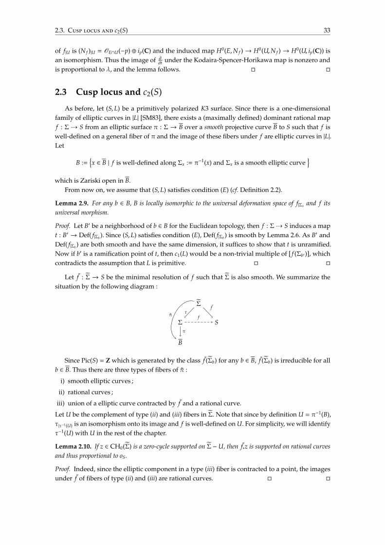
2.3. Cusp locus and c2(S) 33

of f|U is (N f )|U = OE∩U(−p) ⊕ ip(C) and the induced map H0(E,N f ) → H0(U,N f ) → H0(U, ip(C)) isan isomorphism. Thus the image of ∂

∂t under the Kodaira-Spencer-Horikawa map is nonzero andis proportional to λ, and the lemma follows.

2.3 Cusp locus and c2(S)

As before, let (S,L) be a primitively polarized K3 surface. Since there is a one-dimensionalfamily of elliptic curves in |L| [SM83], there exists a (maximally defined) dominant rational mapf : Σ d S from an elliptic surface π : Σ → B over a smooth projective curve B to S such that f iswell-defined on a general fiber of π and the image of these fibers under f are elliptic curves in |L|.Let

B :=x ∈ B | f is well-defined along Σx := π−1(x) and Σx is a smooth elliptic curve

which is Zariski open in B.

From now on, we assume that (S,L) satisfies condition (E) (cf. Definition 2.2).

Lemma 2.9. For any b ∈ B, B is locally isomorphic to the universal deformation space of f|Σx and f itsuniversal morphism.

Proof. Let B′ be a neighborhood of b ∈ B for the Euclidean topology, then f : Σd S induces a mapt : B′ → Def( f|Σb ). Since (S,L) satisfies condition (E), Def( f|Σb ) is smooth by Lemma 2.6. As B′ andDef( f|Σb ) are both smooth and have the same dimension, it suffices to show that t is unramified.Now if b′ is a ramification point of t, then c1(L) would be a non-trivial multiple of [ f (Σb′)], whichcontradicts the assumption that L is primitive.

Let f : Σ → S be the minimal resolution of f such that Σ is also smooth. We summarize thesituation by the following diagram :

Σ

Σ S

B

τπ

f

π

f

Since Pic(S) = Z which is generated by the class f (Σb) for any b ∈ B, f (Σb) is irreducible for allb ∈ B. Thus there are three types of fibers of π :

i) smooth elliptic curves ;

ii) rational curves ;

iii) union of a elliptic curve contracted by f and a rational curve.

Let U be the complement of type (ii) and (iii) fibers in Σ. Note that since by definition U = π−1(B),τ|τ−1(U) is an isomorphism onto its image and f is well-defined on U. For simplicity, we will identifyτ−1(U) with U in the rest of the chapter.

Lemma 2.10. If z ∈ CH0(Σ) is a zero-cycle supported on Σ −U, then f∗z is supported on rational curvesand thus proportional to oS.

Proof. Indeed, since the elliptic component in a type (iii) fiber is contracted to a point, the imagesunder f of fibers of type (ii) and (iii) are rational curves.

34 Chapitre 2. Singularities of curves and Beauville-Voisin zero-cycle

Lemma 2.11. The ramification divisor of f is supported on fibers of π. In particular, the restriction of f ona general fiber of π is an immersion.

The last statement of the above lemma can also be deduced easily from the well-known factthat a general elliptic curve in |L| is nodal since L is primitive.

Proof of Lemma 2.11. If R is the ramification divisor of f , then KΣ is linear equivalent to f ∗KS + R,hence to R since S is a K3 surface. As a general fiber of π is a smooth elliptic curve, KΣ is trivial onthe generic fiber of π. Therefore R is supported on fibers of π.

Remark 2.12. We also deduce that since f ∗c2(S) = c2(Σ) − c2(Q) where Q is the cokernel off ∗ΩS → ΩΣ (because c1(S) = 0), modulo zero-cycles supported on rational curves the secondChern class of S is supported on non-immersive elliptic curves in |L| by Remark 2.10. In fact wewill rather use formula (2.3) in Proposition 2.14 below which is closely related.

In order to analyse the part of c2(S) which is supported on these non-immersive elliptic curves,let us first describe the ramification locus of f|U for (S,L) satisfying condition (E).

Lemma 2.13. If (S,L) satisfies condition (E), then the ramification locus of f|U is reduced, and is supportedon fibers of π whose image under f is a cuspidal elliptic curve.

Proof. Let E be a fiber of π|U : U → B such that f|E is an immersion. Assume that in an analyticneighborhood of z ∈ E, d f : TU→ f ∗TS is given by

(φ1, φ2) : π∗TB × TE→ f ∗TS.

Since f|E is an immersion, φ2 is nonzero. Moreover, since the Def( f|E) is smooth and f|U is theuniversal morphism of Def( f|E) in an analytic neighborhood of E, φ1 |E : π∗TB|E → f ∗TS is therestriction of a nonzero element in H0(E,N f|E ), so det(φ1, φ2) is not identically zero. Hence f isunramified at immersive fibers.

If f|E ramifies at z, then f (E) is a curve with one cusp. By Lemma 2.9 we can work with localcoordinates (2.2) (x, y) in U at z ∈ E so that the first projection coincides with π and that f is givenby

(x, y) 7→(x + y2, y3 +

32

xy)

in these local coordinates. We immediately verify that the ramification divisor along E is reduced.

For all p ∈ B, let Σp denote the fiber of π over p. Since a general member of the family of ellipticcurves determined by |L| is a nodal curve, the points z ∈ U such that f (z) is a cusp in f (Σπ(z)) forma discrete set Zcusp ⊂ U ; we define the cusp locus to be the zero-dimensional reduced subscheme ofU whose underlying set is Zcusp.

Proposition 2.14. The following identity holds in CH0(S)/ZoS

(deg f ) · c2(S) = f∗[Zcusp]. (2.3)

Proof. Recall that the fibers of π in U are smooth elliptic curves, so c1(ΩU/B) = π∗L for someL ∈ Pic(B). Since c1( f ∗TS)|U = 0, one has

c2( f ∗TS)|U = c2

(ΩU/B ⊗

(f ∗TS

)|U

),

2.4. Double point locus 35

which is determined by the scheme-theoretic vanishing locus V(s) of the section s of ΩU/B ⊗ f ∗|UTS

induced by d f : TU → f ∗|UTS. Suppose that f is given by (x, y) 7→ (1(x, y), h(x, y)) in a local

coordinates near p ∈ U such that the first projection x 7→ (x, y) coincides with π : Σ→ B. Then thedegree of c2( f ∗

|UTS) supported on p is equal to the vanishing order at (0, 0) of (x, y) 7→ (∂y1, ∂yh),which is 0 if fπ(p) := f|Σπ(p) is an immersion at p.

If fπ(p) ramifies at p, then f (p) is a cusp of f (Σπ(p)) by hypothesis. Using local coordinates (2.2)at p, the map f is given by

(x, y) 7→(x + y2, y3 +

32

xy).

This implies that the length of V(s) at p is 1, so c2( f ∗|UTS) = [Zcusp] in CH0(U). Hence by Lemma 2.10

(deg f ) · c2(S) = f∗ f ∗c2(S) = f∗([Zcusp]

)in CH0(S)/ZoS.

In the next section, we will give a rigorous definition for other important zero cycles appearingnaturally in the geometry of the map f . Let us describe them in simple terms : the curves f (Σb)are nodal, so each curve Σb contains two points over each node of f (Σb). These points fill in acurve C which roughly speaking is the double point locus of f . There is an involution i on thiscurve exchanging the two points over the same node. Furthermore, there is a morphism of vectorbundles (to be defined more carefully later on)

TΣ/B |C ⊕ i∗TΣ/B |C → ( f ∗TS)|C.

Obviously, the determinant of this morphism vanishes at cuspidal points. The vanishing locus ofthis determinant will be analyzed carefully in the last section.

2.4 Double point locus

In this section, we will first define rigorously the double point locus C of f and its involutionσ. We would like to consider Zcusp as the invariant subscheme of C under the involution map σ(see Lemma 2.19). However it does not work if this double point locus C is defined in U, since theinvolution σ is not well-defined everywhere, for instance on the pre-images of points of multiplicitygreater than 2 of an elliptic curve in |L|.

To this end, we first introduce the surface U1, which is defined as the residual scheme to ∆U inU×S U ⊂ U×U, where ∆U is the diagonal of U×U (we refer to [Ful98, Chapter 9] for the definitionand cycle-theoretic properties of residual schemes). Then we will define the double point locus Cas being contained in U1 (which is different from the usual definition as in [Ful98, Chapter 9]).

First of all, as a consequence of hypothesis (E), we note that

Lemma 2.15. U1 is a surface which is smooth in an analytic neighborhood of R := U1 ∩ ∆U.

Proof. By definition, R is the ramification locus of ∆U ' U→ S, which by Lemma 2.11 is reducedand consists of fibers of π whose image under f contains a cusp. Let E be one of these fibersand z be a point in E. Suppose first that f|E is unramified at z. Since the ramification divisor off|U is reduced, there exist local coordinates (x, y) of z ∈ U such that the first projection coincideswith π and that f is given by (x, y) 7→

(x2, y

). This is because we can first suppose that locally the

ramification locus of f is the line V(x = 0) ⊂ S. So if f is locally given by (x, y)→(x · φ(x, y), ψ(x, y)

),

36 Chapitre 2. Singularities of curves and Beauville-Voisin zero-cycle

since jac f = x it is easy to see that φ = x · h(x, y) with h(0, 0) , 0 and that dψ is invertible at (0, 0).Passing to the local chart of S given by the inverse of (x, y) 7→ (x

√h, ψ) allow to conclude.

Taking another copy of (x, y) gives local coordinates (x, y, x′, y′) around (z, z) ∈ U × U, thenlocally at (z, z), the equations defining U ×S U ⊂ U × U is (x + x′)(x − x′) = y − y′ = 0. Since thediagonal is given by x − x′ = y − y′ = 0, one deduces that U1 is given by x + x′ = y − y′ = 0. HenceU1 is smooth at (z, z).

If f|E ramifies at z, using the local coordinates (2.2), the equations defining U×S U at (z, z) ∈ U×Uare given by x + y2 = x′ + y′2

y3 + 32 xy = y′3 + 3

2 x′y′(2.4)

The first equation defines a smooth hypersurface in U×U. After eliminating x′ by the first equation,the second equation becomes

(y − y′)(y2 + yy′ + y′2 +

32(x − y′(y + y′)

))= 0.

So the residual scheme U1 is locally defined in C3 by

y2 + yy′ + y′2 +32(x − y′(y + y′)

)= 0.

Hence U1 is smooth at (z, z).

Let p1 and p2 denote the two projections of U1 ⊂ U × U to each component. For i = 1, 2, letπi := π pi. We define the double point locus of f , denoted by C, to be the residual scheme to R in(π1, π2)−1(∆B) = U×S U∩U×B U. The involution exchanging the two components of U×U inducesan involution σ on C. The invariant subscheme of C under σ is denoted by Cσ.

Lemma 2.16. For i = 1, 2,

(i) pi : U1 → U is a finite morphism ;

(ii) The restriction of πi : U1 → B to C is finite.

Proof. For (i), suppose that pi is not finite, then there is a curve D in U such that f (D) is a point.Since f does not contract fibers of π, D has to dominate B, which contradicts Lemma 2.11.

Next, assume that C ∩ π−1i (b) has positive dimension for some b ∈ B. Since pi is finite by (i), the

image of C∩π−1i (b) under pi is the curve E := Σb. By definition of C, this implies that f|E is of degree

> 1 onto its image and contradicts the hypothesis Pic(S) = Z · L.

Lemma 2.17. U1 is smooth along C. In particular, C is a Cartier divisor in U1.

Remark 2.18. That C is a Cartier divisor in U1 is in fact a direct consequence of Lemma 2.15. Indeed,this follows from the fact that (π1, π2)−1(∆B) is a Cartier divisor in U1, and that U1 is smooth alongR.

Proof of Lemma 2.17. Let (z, z′) ∈ C ⊂ U1. If z = z′, then U1 is smooth along (z, z′) by Lemma 2.15.Suppose that z , z′ ; since (S,L) satisfies hypothesis (E), either z, z′ ∈ U do not lie in the ramificationdivisor of f , or z, z′ ∈ U belong to the ramification divisor of f and the local images of Σπ(z) at z andat z′ under f (denoted f (γz) and f (γz′)) intersect transversally at f (z). In the first case, since anynon-zero element in H0(Σπ(z),N f ) vanishes nowhere on Σπ(z) and f|Σπ(z) is an immersion, f defines a

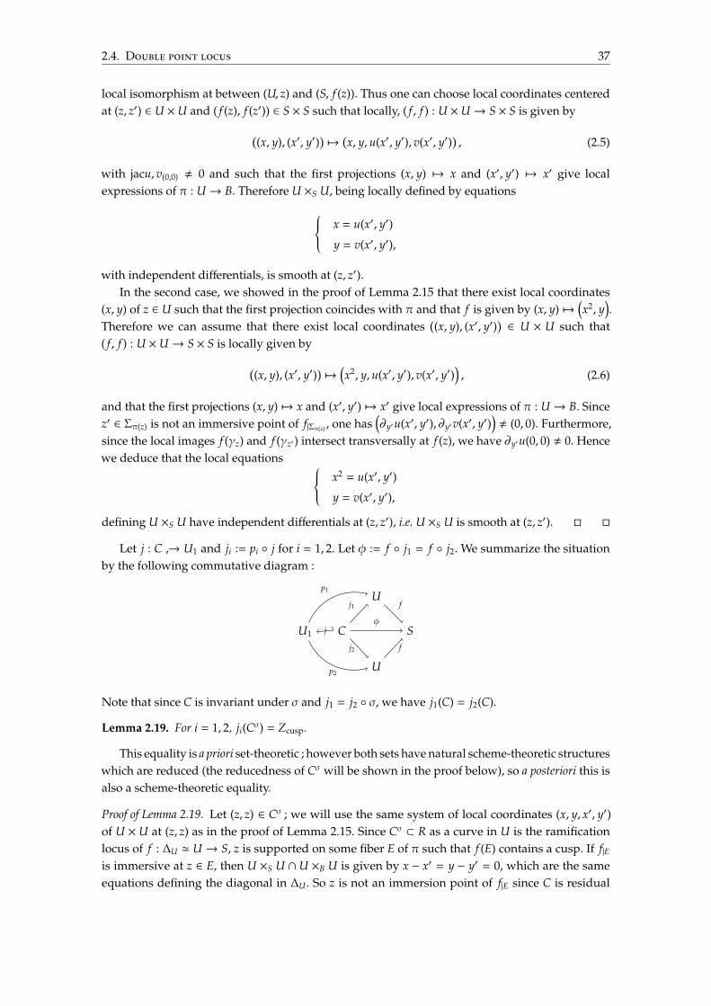
2.4. Double point locus 37

local isomorphism at between (U, z) and (S, f (z)). Thus one can choose local coordinates centeredat (z, z′) ∈ U ×U and ( f (z), f (z′)) ∈ S × S such that locally, ( f , f ) : U ×U→ S × S is given by(

(x, y), (x′, y′))7→

(x, y,u(x′, y′), v(x′, y′)

), (2.5)

with jacu, v(0,0) , 0 and such that the first projections (x, y) 7→ x and (x′, y′) 7→ x′ give localexpressions of π : U→ B. Therefore U ×S U, being locally defined by equations x = u(x′, y′)

y = v(x′, y′),

with independent differentials, is smooth at (z, z′).In the second case, we showed in the proof of Lemma 2.15 that there exist local coordinates

(x, y) of z ∈ U such that the first projection coincides with π and that f is given by (x, y) 7→(x2, y

).

Therefore we can assume that there exist local coordinates((x, y), (x′, y′)

)∈ U × U such that

( f , f ) : U ×U→ S × S is locally given by((x, y), (x′, y′)

)7→

(x2, y,u(x′, y′), v(x′, y′)

), (2.6)

and that the first projections (x, y) 7→ x and (x′, y′) 7→ x′ give local expressions of π : U→ B. Sincez′ ∈ Σπ(z) is not an immersive point of f|Σπ(z) , one has

(∂y′u(x′, y′), ∂y′v(x′, y′)

), (0, 0). Furthermore,

since the local images f (γz) and f (γz′ ) intersect transversally at f (z), we have ∂y′u(0, 0) , 0. Hencewe deduce that the local equations x2 = u(x′, y′)

y = v(x′, y′),

defining U ×S U have independent differentials at (z, z′), i.e. U ×S U is smooth at (z, z′).

Let j : C → U1 and ji := pi j for i = 1, 2. Let φ := f j1 = f j2. We summarize the situationby the following commutative diagram :

U

U1 C S

U

j1

j2

f

f

φ

p1

p2

j

Note that since C is invariant under σ and j1 = j2 σ, we have j1(C) = j2(C).

Lemma 2.19. For i = 1, 2, ji(Cσ) = Zcusp.

This equality is a priori set-theoretic ; however both sets have natural scheme-theoretic structureswhich are reduced (the reducedness of Cσ will be shown in the proof below), so a posteriori this isalso a scheme-theoretic equality.

Proof of Lemma 2.19. Let (z, z) ∈ Cσ ; we will use the same system of local coordinates (x, y, x′, y′)of U × U at (z, z) as in the proof of Lemma 2.15. Since Cσ ⊂ R as a curve in U is the ramificationlocus of f : ∆U ' U → S, z is supported on some fiber E of π such that f (E) contains a cusp. If f|Eis immersive at z ∈ E, then U ×S U ∩ U ×B U is given by x − x′ = y − y′ = 0, which are the sameequations defining the diagonal in ∆U. So z is not an immersion point of f|E since C is residual

38 Chapitre 2. Singularities of curves and Beauville-Voisin zero-cycle

to ∆U. Therefore, ji(z, z) is supported on Zcusp. Working in local coordinates (2.2), the system ofequations that defines (U ×S U) ∩ (U ×B U) at (z, z) is

x = x′

x + y2 = x′ + y′2

y3 + 32 xy = y′3 + 3

2 x′y′(2.7)

So the equation defining C, being the residual scheme to R in (U ×S U) ∩ (U ×B U), isx = x′

y = −y′

32 x − y2 = 0

(2.8)

and in the coordinates (x, y) the involution σ acts on C by (x, y) 7→ (x,−y). So locally Cσ is thereduced point (0, 0), hence ji(Cσ) = Zcusp.

Lemma 2.20. The scheme-theoretic intersection C ∩ R is Cσ.

Proof. It is clear from the system of local equations 2.7 and 2.8 describing (U ×S U) ∩ (U ×B U) andC in the proof of Lemma 2.19.

Next we defineψ : j∗1TU/B ⊕ j∗2TU/B → φ∗

|CTS (2.9)

to be the sum of j∗i TU/B → φ∗|CTS induced by TU/B → f ∗

|UTS. Let W be the Cartier divisor of Cdefined by the vanishing of detψ. The geometry motivation for introducing ψ and W is the factthat away from the ramification of f , the vanishing locus of detψ consists of pairs (z, z′) such thatthe local branches f (γz) and f (γz′) do not intersect transversally. As we will see in the proof ofProposition 2.21, the length of W over (z, z′) is precisely one less the intersection multiplicity off (γz) and f (γz′). The zero cycle W will play a key role in the conclusion of the proof in the nextsection.

2.5 Proof of Theorem 2.3

Since we are dealing with algebraic cycles on varieties which are not necessarily smooth, it willbe convenient to introduce the homomorphism

τ : K0(X)→ CH∗(X)Q

constructed in [Ful98, Theorem 18.3] by MacPherson [Mac74] for any algebraic scheme X. (Oneshould think to τ as extending the map F 7→ ch(F ) · Td(X) defined for smooth X.)

The properties of τ that we need is the following, which can be found in [Ful98, Theorem 18.3] :• τ defines a homomorphism of K0(X)-modules in the sense that for any α ∈ K0(X) and anyβ ∈ K0(X), one has

τ(β ⊗ α) = ch(β) · τ(α);

• If supp(F ) is a zero-dimensional subscheme of X, then

τ(F ) =∑

x∈supp(F )

lx(F )[x] ∈ CH0(X)Q,

2.5. Proof of Theorem 2.3 39

where lx(F ) denotes the length of the stalk of F over the local ring OX,x.• If f : X→ Y is a local complete intersection morphism, then

τ( f ∗α) = td(T f ) · f ∗τ(α)

for any α ∈ K0(Y) where T f ∈ K0(X) stands for the virtual tangent bundle.Let ΩC/B be the relative cotangent with respect to π1 |C = π2 |C : C → B. Since π1 |C is a finite

morphism between curves by Lemma 2.16, ΩC/B is supported on a zero-dimensional subscheme.Therefore

τ(ΩC/B) =∑

x∈supp(ΩC/B)

lx(ΩC/B)[x] ∈ CH0(C)Q.

Back to the morphism ψ we defined in (2.9), we can describe the zero locus of detψ as follows :

Proposition 2.21. Let W ⊂ C be the zero locus of detψ, then [W] ∈ π1∗

|CPic(B) ⊂ CH0(C). Moreover, thefollowing identity holds in CH0(C)Q

τ(ΩC/B) + [Cσ] = [W]. (2.10)

Proof. Since W is the scheme-theoretic vanishing locus ofψ : j∗1TU/B⊕ j∗2TU/B → φ∗|CTS and c1(TS) = 0,

its cycle class [W] in CH0(C) is given by

[W] = c1( j∗1ΩU/B ⊕ j∗2ΩU/B)

= j∗1c1(ΩU/B) + j∗2c1(ΩU/B).

The first statement of Proposition 2.21 follows from the fact that c1(ΩU/B) ∈ π∗Pic(B).Since Cσ is reduced, to show that τ(ΩC/B) + [Cσ] = [W], it suffices to show that for all closed

points x ∈ C, lx(W) = 1 + lx(ΩC/B) if x ∈ Cσ;

lx(W) = lx(ΩC/B) otherwise.

Suppose that z = z′, i.e. (z, z′) ∈ Cσ (that is, we are in the cusp situation leading to vanishing ofψ). On one hand, using local coordinates (2.2) to give local coordinates (x, y, x′, y′) of U×U at (z, z),we have in the proof of Lemma 2.19 the system of equations (2.8)

x = x′

y = −y′

32 x − y2 = 0

(2.11)

defines the curve C at (z, z′). After eliminating the variables x′ and y′, locally the curve C is givenby 3

2 x − y2 = 0. Since C→ B is locally the first projection of (x, y), we deduce that lz,z′ (ΩC/B) = 1On the other hand, by simple computations detψ is given by

(x, y, x′, y′) 7→ yy′(2y′ − 2y + x′ − x

).

After eliminating x′, y′ and dividing out y−y′ (since C is residual to ∆U), detψ becomes (x, y) 7→ −y2.Hence l(z,z′)(W) = 2.

Now assume that z , z′. Recall first that (z, z′) ∈ C if and only if there exists an elliptic curve Σb

40 Chapitre 2. Singularities of curves and Beauville-Voisin zero-cycle

with z, z′ ∈ Σb and f (z) = f (z′). On the other hand by Lemma 2.11, the ramification of f is a unionof curves Σb, so either none of z, z′ belongs to the ramification divisor of f , or both.

1) First we suppose that z, z′ ∈ U do not lie in the ramification divisor of f : U→ S. In this case,as we showed in the proof of Lemma 2.17, the local expression of ( f , f ) : U ×U → S × S is givenby (2.5) :

(x, y, x′, y′) 7→ (x, y,u(x′, y′), v(x′, y′)).

So the equations defining C are x = x′

x = u(x′, y′)

y = v(x′, y′).

After eliminating the variables x and y by the first and the third equations, the curve C is definedby the vanishing of 1(x′, y′) := x′ − u(x′, y′) in the local coordinates (x′, y′). On one hand, sinceπ : U→ B is locally given by the first projection (x′, y′) 7→ x′, we obtain the following isomorphismof OC,(z,z′)-algebras :

(ΩC/B)(z,z′) '(C[x′, y′]/(1, ∂y′1)

)(x′,y′)

.

On the other hand, in these local coordinates, up to sign detψ can be written as

detψ(x′, y′) = ∂y′u(x′, y′) = ∂y′1(x′, y′).

Hence as OC,(z,z′)-algebras,OW,(z,z′) '

(C[x′, y′]/(1, ∂y′1)

)(x′,y′)

.

In particular, l(z,z′)(W) = l(z,z′)(ΩC/B).

2) Still assuming z , z′, it remains to treat the case where z, z′ ∈ U lie in the ramification divisorof f : U → S. It is easy to see that under these assumptions, (z, z′) < W. Indeed, if (z, z′) ∈ C isa point where detψ vanishes, this means that the two spaces ( f|E)∗(TE,z) and ( f|E)∗(TE,z′) generateat most a one-dimensional subspace of TS, f (z) where E ⊂ U is the elliptic curve passing throughz, z′ ∈ U. But since S satisfies condition (E), either φ(z, z) is the cusp of the elliptic curve f (Σπ(z))hence z = z′, or z, z′ ∈ U do not lie in the ramification divisor of f : U → S, which all violate ourassumptions. Hence we need to show that ΩC/B is not supported on (z, z′) to finish the proof.

Using local expressions (2.6) given in the proof of Lemma 2.17, the equations defining C arex = x′

x2 = u(x′, y′)

y = v(x′, y′).

So the curve C is defined by the vanishing of x′2 − u(x′, y′) in the local coordinates (x′, y′). Sinceπ : U→ B is locally given by the first projection (x′, y′) 7→ x′, we deduce that

(ΩC/B)(z,z′) '(C[x′, y′]/(x′2 − u, ∂y′u)

)(x′,y′)

as OC,(z,z′)-algebras. Recall in the proof of Lemma 2.17 that since f|E(γz) and f|E(γz′) intersecttransversally, one has ∂y′u(0, 0) , 0. Therefore, ΩC/B is not supported on (z, z′).

2.5. Proof of Theorem 2.3 41

Lemma 2.22. The following identity holds in CH0(C)Q :

τ(ΩC/B) = c1( j∗ΩU1 ) + j∗[C] − j∗1c1(π∗ΩB). (2.12)

Proof. First of all, since π∗1 |C is a finite morphism by Lemma 2.16 and since π∗1 |CΩB is torsion-free,the cotangent sequence

0 π∗1 |CΩB ΩC ΩC/B 0

is exact on the left. On the other hand, since C is a Cartier divisor on the smooth surface U1, theconormal exact sequence

0 OC(−C) j∗ΩU1 ΩC 0

is also exact on the left. Therefore, if we write τ(OC) = [C] + ξ for some ξ ∈ CH0(C)Q, we have

τ(ΩC/B) = τ( j∗ΩU1 ) − τ(OC(−C)) − τ(π∗1 |CΩB)

=(ch( j∗ΩU1 ) − ch(OC(−C)) − ch(π∗1 |CΩB)

)· ([C] + ξ)

= c1( j∗ΩU1 ) + j∗[C] − c1(π∗1 |CΩB),

which finishes the proof.

Lemma 2.23. The following equality holds in CH0(C)Q :

c1(ΩU1 |C) = j∗1c1(ΩU) + j∗2c1(ΩU) − j∗[R]. (2.13)

Proof. First of all, since p1 : U1 → U is finite and U is smooth, p∗1ΩU → ΩU1 is injective. Next, sincep∗2ΩU/S =

(ΩU×SU/U

)|U1

and ΩU×SU |U1= ΩU1 (R), one has p∗2ΩU/S = ΩU1 (R)/p∗1ΩU. So

c1( j∗p∗2ΩU/S) = c1(ΩU1 |C) + j∗[R] − j∗p∗1c1(ΩU)

in CH0(C). Finally since f ∗ΩS → ΩU is injective and since j2 = p2 j is a local complete intersectionmorphism (indeed, j2 factorizes through C → U × U → U where the first arrow is the closedembedding of C into U ×U and the second arrow is the projection onto the second factor, which isa smooth morphism), we deduce that in CH0(C)Q,

td(T j2 ) · j∗2(τ( f ∗ΩS) − τ(ΩU) + τ(ΩU/S)

)= 0

If we write td(T j2 ) = [C] + ξ′ for some ξ′ ∈ CH0(C)Q, then we get

c1( j∗2ΩU/S) = j∗2(c1(ΩU) − f ∗c1(ΩS)

)= j∗2c1(ΩU)

in CH0(C)Q. Hence the identity (2.13) is proven.

Recall from the definition of C that [C] = [(π1, π2)−1(∆B)] − [R] ; for simplicity, we now define

C′ := (π1, π2)−1(∆B). (2.14)

42 Chapitre 2. Singularities of curves and Beauville-Voisin zero-cycle

Combining equalities (2.12) and (2.13), we obtain

τ(ΩC/B) = j∗1c1(ΩU) + j∗2c1(ΩU) − j∗1c1(π∗ΩB) + j∗[C′] − 2 j∗[R]. (2.15)

From now on, we fix a 1-cycle α ∈ CH1(Σ) such that α|U = ( ji)∗[C] for i = 1, 2. The followingresult is the key point of the whole computation.

Lemma 2.24. There exists a 1-cycle V ∈ CH1(Σ) supported on fibers of π : Σ→ B such that α = V + f ∗Lin CH1(Σ)Q.

Proof. Let U ⊂ B be the Zariski open set parameterizing nodal elliptic curves in |L|. Since j1(C)∩Σx

is the double point locus (defined in [Ful98, Chapter 9]) of the restriction of f to Σx, its classin CH0(Σx) is equal to

(f ∗ f∗[Σx]

)|Σx

=(

f ∗L)|Σx

by the double point formula [Ful98, Theorem 9.3](Since KS and KΣx are trivial). The lemma follows from the "spreading principle" [Voi14, Theorem1.2].

Corollary 2.25. If D ∈ CH1(Σ) is a 1-cycle supported on the fibers of π : Σ→ B, then f∗(α ·D) ∈ CH0(S)Q

is proportional to oS, or equivalently f∗(α ·D) = 0 in CH0(S)Q/QoS.

Proof. By Lemma 2.24, we havef∗ (α ·D) = L · f∗D,

because D · V = 0 and by the projection formula. So f∗ (α ·D) = 0 in CH0(S)Q/QoS by Theorem 2.1(i).

Using Corollary 2.25, we will prove the two following lemmata :

Lemma 2.26.

i) There exists a zero-cycle z ∈ CH0(Σ) whose restriction to U is ( j1)∗ j∗1c1(π∗ΩB) such that f∗z = 0 inCH0(S)Q/QoS.

ii) There exists zero-cycles zi ∈ CH0(Σ) for i = 1, 2 whose restrictions to U is ( ji)∗ j∗i c1(ΩU) such thatf∗zi = 0 in CH0(S)Q/QoS.

Proof. Since α|U = ( j1)∗[C], the restriction to U of z := α · π∗c1(ΩB) ∈ CH0(Σ) is ( j1)∗ j∗1c1(π∗ΩB).Applying Corollary 2.25 to D = π∗c1(ΩB) allows to conclude. The same argument applied tozi := α · c1(ΩΣ) proves the lemma for ( ji)∗ j∗i c1(ΩU), since c1(ΩΣ) is supported on fibers of π : Σ →

B.

Recall that C′ is defined in (2.14).

Lemma 2.27. There exists a zero-cycle z′ ∈ CH0(Σ) whose restriction to U is ( j1)∗ j∗ ([C′]) such thatf∗z′ = 0 in CH0(S)Q/QoS.

Proof. Let pr1 : U ×U→ U be the first projection, then the following holds in CH0(U) :

( j1)∗ j∗ ([C′]) = (p1)∗ ([C] · [C′])

= (pr1)∗(p1, p2)∗((p1, p2)∗(π, π)∗[∆B] · [C]

)= (pr1)∗

((π, π)∗[∆B] · (p1, p2)∗[C]

).

2.5. Proof of Theorem 2.3 43

Now let jU be the inclusion map of the diagonal ∆U → U ×U, one has

(pr1)∗((π, π)∗[∆B] · (p1, p2)∗[C]

)= pr1∗ jU∗

(jU∗(π, π)∗[∆B] · (pr1 jU)−1

∗ ( j1)∗[C])

=(pr1 jU

)∗

(jU∗(π, π)∗[∆B]

)· ( j1)∗[C].

Since

∆U U ×U U

∆B B × B B

jU pr1

pr1

πjB

π(π, π)

is a Cartesian diagram, the left square shows that jU∗(π, π)∗[∆B] = π∗b0 for some b0 ∈ CH0(∆B). So viathe isomorphisms pr1 jU and pr1 jB in the above Cartesian diagram, if b :=

(pr1 jB

)∗b0 ∈ CH0(B),

then (pr1 jU

)∗

jU∗(π, π)∗[∆B] = π∗b.

Therefore,

( j1)∗ j∗ ([C′]) =(pr1 jU

)∗

(jU∗(π, π)∗[∆B]

)· ( j1)∗[C] = π∗b · ( j1)∗[C].

Let z′ := α · π∗b ; we conclude by applying Corollary 2.25 to the 1-cycle D = π∗b.

Corollary 2.28. The following equality modulo zero-cycles supported on rational curves holds in CH0(S)Q/QoS :

f∗τ(ΩC/B) = −2 f∗ ([C] · [R]) = −2 f∗( j1)∗ ([Cσ]) . (2.16)

Before we start the proof, we need to clarify the meaning of the above equalities, whichhave to be understood using Lemma 2.10 as follows : for any zero-cycle ξ ∈ CH0(U), we define

f∗ξ ∈ CH0(S)Q/QoS to be f∗β modulo QoS for any zero-cycle β ∈ CH0(Σ)Q such that β|U = ξ.This definition is independent of the choice of β by virtue of Lemma 2.10, hence the identities inCorollary 2.28 do make sense.

Proof of Corollary 2.28. Note that the second equality results directly from Lemma 2.20. Sincef j1 = f j2, we deduce from Lemmata 2.26 and 2.27 that

f∗( j1)∗(j∗1c1(ΩU) + j∗2c1(ΩU) − j∗1c1(π∗ΩB) + j∗[C′]

)= f∗ (z1 + z2 − z + z′) = 0

in CH0(S)Q/QoS. Now the corollary follows easily from equality (2.15).

We finish the proof of Theorem 2.3 as follows :

Proof of Theorem 2.3. By Proposition 2.21, there exists a 1-cycle D supported on the fibers of π :Σ→ B such that [W] is the restriction of α ·D to U. Thus by Corollary 2.25, we have f∗[W] = 0 inCH0(S)Q/QoS. So we deduce from equality (2.10) that

f∗τ(ΩC/B) = − f∗( j1)∗[Cσ] in CH0(S)Q/QoS.

This identity together with equality (2.16) give

f∗( j1)∗[Cσ] = 0 in CH0(S)Q/QoS.

44 Chapitre 2. Singularities of curves and Beauville-Voisin zero-cycle

By Lemma 2.19,f∗[Zcusp] = f∗( j1)∗[Cσ] in CH0(S)Q/QoS.

Finally by Proposition 2.14, we conclude that c2(S) is proportional to f∗[Zcusp] = 0 in CH0(S)Q/QoS.

We finish this section by stating the following corollary (already appeared in the proof of Theo-rem 2.3), which can be considered either as a consequence of Proposition 2.21 and Corollary 2.28,or of Theorem 2.1 and Proposition 2.14.

Corollary 2.29. Let (S,L) be a primitively polarized K3 surface satisfying hypothesis (E). The push-forwardunder f of the class modulo rational equivalence of the cusp locus Zcusp is proportional to the Beauville-Voisinzero-cycle oS.

Chapitre 3

Rational maps from punctual Hilbertschemes of K3 surfaces

Résumé

Le but de ce chapitre est d’étudier les applications rationnelles dominantes d’un schéma deHilbert ponctuel de longueur k ≥ 2 d’une surface K3 projective S. Précisément, nous démontronsque leur image est rationnellement connexe si cette application rationnelle n’est pas génériquementfinie. Comme application, nous simplifions la preuve de C. Voisin du fait que les involutionssymplectiques d’une surface K3 projective S agissent trivialement sur le groupe de Chow deszéro-cycles de S

Abstract

The purpose of this chapter is to study dominant rational maps from a punctual Hilbert schemeof length k ≥ 2 of a projective K3 surfaces S. Precisely, we prove that their image is rationallyconnected if this rational map is not generically finite. As an application, we simplify C. Voisin’sproof of the fact that symplectic involutions of any projective K3 surface S act trivially on the Chowgroup of zero-cycles of S.

3.1 Introduction

Recall that a K3 surface S is by definition a smooth projective surface with trivial canonicalbundle KS = Ω2

S and vanishing H1(S,OS). The Hilbert scheme of zero-dimensional subschemes oflength k ≥ 2 on the K3 surface S will be denoted by S[k].

Recall that a proper variety X is said to be uniruled (resp. rationally connected) if a generalpoint x ∈ X (resp. two general points x, y ∈ X) is contained in the image of a non-constant mapP1→ X. These are obviously birationally invariant properties. It is also clear that CH0(X) = Z

for any rationally connected variety X. When X is smooth, rational connectedness is equivalentto the a priori weaker condition that two general points can be joined by a chain of rationalcurves [KMM92b, Theorem 2.1].

The following is the main result we obtain in this chapter :

Theorem 3.1. If f : S[k] d B is a dominant rational map to a variety B with dim B < dim S[k], then eitherB is a point or rationally connected.

46 Chapitre 3. Rational maps from K3[n]

This theorem will be generalized after in Chapter 4, but here we give a more elementary proofin this particular case. As an application of Theorem 3.1, we will simplify the proof of C. Voisin’smain result in [Voi12b].

Theorem 3.2 (Voisin). Suppose S is a projective K3 surface and ı is a symplectic involution acting on S,then ı acts as the identity on CH0(S).

The motivation for the statement of Theorem 3.2 comes from the following conjecture, whichis a consequence of the generalized Bloch conjecture for surfaces :

Conjecture 3.3. If S is a surface with q = h0,1 = 0 and f : S→ S is an automorphism of finite order actingtrivially on H0(S,Ω2

S), then the induced map f∗ acts as the identity on CH0(S).

A series of examples of surfaces with q = 0 is provided by K3 surfaces S. Such surfaceshave one-dimensional H0(S,Ω2

S) generated by a non-degenerated holomorphic two-form η. Anautomorphism f : S→ S such that f ∗η = η is called a symplectic automorphism.

A recent new advance of Conjecture 3.3 for K3 surfaces was made by D. Huybrechts and M.Kemeny in [HK13]. They worked with invariant elliptic curves and solved Conjecture 3.3 for K3surfaces with symplectic involutions f in one of the three series in the classification introduced byvan Geemen and Sarti [BvG07]. In [Voi12b], C. Voisin showed in general that symplectic involutionsact trivially on CH0(S) for any projective K3 surface S. The general statement of Conjecture 3.3 forK3 surfaces is proved soon after in [Huy12] by D. Huybrechts.

Theorem 3.4 (Kemeny-Huybrechts, Voisin). Let S be a projective K3 surface, η be a non-zero holomorphictwo-form on S, and f : S → S be a symplectic automorphism of finite order on S, then f acts trivially onCH0(S).

As was shown by Nikulin in [Nik80], the only possible orders of f range from one to eight.In Huybrechts’ proof, he studied case by case according to these finitely many possible ordersusing derived technique and Garbagnati and Sarti’s classification results [GS07] on lattices of theinvariant part H2(X,Z) f of the action of symplectic automorphism f with prime order.

The main construction in Voisin’s proof [Voi12b] of Theorem 3.2 is the factorization

S[1] CH0(S)

P(S,H)(C /C )γS

Γ∗

(3.1)

where P(S,H)(C /C ) is the universal Prym variety associated to a complete linear system of curvesof genus 1 in the quotient surface S/ı. Details of the above construction will be given in Section 3.4.Our main application of Theorem 3.1 is the following

Theorem 3.5. Any smooth projective compactification of P(S,H)(C /C ) is rationally connected.

The organization of this chapter is as follows. In Section 3.2, we will recall some well-knownfacts concerning rationally connected varieties and use them to reformulate Theorem 3.1. Then wewill prove Theorem 3.1 in Section 3.3. In Section 3.4, we will explain how Theorem 3.5 gives analternative proof of Theorem 3.2.

3.2. Remarks on rationally connected varieties 47

3.2 Remarks on rationally connected varieties

In this section, we first recall the definition of MRC-fibrations and introduce the main theoremof Graber-Harris-Starr in [GHS03]. Then we will use them to give a reformulation of Theorem 3.1.

Recall from [KMM92b] that for any variety X, there exists a rational map φ : Xd B unique upto birational equivalence characterized by the following properties :

(i) a general fiber of φ is rationally connected ;

(ii) for a general point b ∈ B, any rational curve passing through Xb := φ−1(b) is actually containedin Xb.

The map φ : X d B is called the maximal rationally connected (or MRC for short) fibration of X.The fundamental question whether the base B of an MRC-fibration is not uniruled remained openfor a while [Kol96, Conjecture IV.5.6]. It was finally answered by T. Graber, J. Harris, and J. Starras a direct corollary of their main theorem in their paper [GHS03] :

Theorem 3.6 (Graber-Harris-Starr). Let 1 : X → C be a proper morphism between complex varietieswhere C is a smooth curve. If the general fiber of 1 is rationally connected, then 1 has a section.

Remark 3.7. This theorem was later generalized by Starr and de Jong to varieties defined overan arbitrary algebraically closed field : any proper morphism from a smooth variety to a smoothcurve whose general fibers are smooth and separably rationally connected has a section [dJS03].

In particular, Theorem 3.6 implies :

Corollary 3.8 (Graber-Harris-Starr [GHS03]). Let 1 : Xd Z be a maximal rationally connected fibrationwhere X is an irreducible variety, then Z is not uniruled.

Let us recall for completeness the proof of the above corollary.

Proof. After resolving the rational map 1 and singularities of X, we can assume that 1 is a morphismand X is smooth. Suppose that Z were uniruled, then there exists a rational curve C passing througha general point of Z and we can suppose that 1 is dominant on C. Denote by C the normalizationof C. Up to replacing X ×Z C by its desingularization, the map 1C : X ×Z C→ C has a section D byTheorem 3.6, which is also a rational curve. Thus if y ∈ D, the rational curve D passes through yand is not contracted by 1, which is absurd because 1 : X→ Z is an MRC-fibration.

Remark 3.9. An equivalent formulation of Corollary 3.8 is the following : if f : X d B is adominant map such that both the general fibers of f and the base B are rationally connected, thenX is rationally connected as well [Kol96, Proposition IV.5.6.3].

Thanks to Corollary 3.8, we can easily show that

Corollary 3.10. In Theorem 3.1, it is equivalent to show that B is either a point or uniruled.

Proof. Only one direction needs to be proved. Assume that Theorem 3.1 is true when replacing"rationally connected" with "uniruled". Suppose B is not a point ; let Bd B′ be an MRC fibrationof B. Since B′ is not uniruled by Corollary 3.8, we deduce that B′ is a point by assumption. HenceB is rationally connected.

48 Chapitre 3. Rational maps from K3[n]

3.3 Proof of Theorem 3.1

Let us first prove the following general result.

Lemma 3.11. Let f : X d B be a rational dominant map between smooth projective varieties such thatdim X > dim B. If D is an ample divisor on X, then the restriction map f|D is still dominant provided B isnot uniruled.

Remark 3.12. The following example shows that the hypothesis of B not being uniruled is essentialin the above lemma. Let l be a line in P2 and p a point in P2 which is not contained in l. If f : P2 d lis the projection from p, then f is dominant and every line in P2 containing p is contracted to apoint under f .

Remark 3.13. Before we start the proof, we remark that any birational modification of the rationalmap f : S[k] d B and the base B will not affect the hypotheses and the conclusion in Theorem 3.1.For instance up to desingularization of B, we can always suppose that B is smooth and complete.This kind of modification will be repeatedly used in the proof of Theorem 3.1.

Proof of Lemma 3.11. Let f : X→ B be a resolution of f after a sequence of blow-ups π : X→ X ofX. Denote by D the proper transform of D and D′ := π−1(D). Since D is ample and [D′] = π∗[D] inPic(X), one deduces that D′ is a big divisor. Suppose k = dim X−dim B and denoted by H ∈ NS(X)the class of an ample divisor on X. As f is dominant, the class f ∗[x] · Hk−1

∈ NS(X), where x is apoint of B, is a class of a movable curve. So [D′] · f ∗[x] · Hk−1 > 0 [BDPP13, Corollary 2.5], hencethe restriction f|D′ is dominant.

Now let y be a very general point of B such that there is no rational curve passing through y.We know that there exists x ∈ D′ such that y = f (x). As π(x) ∈ D, the fiber Ex := π−1(π(x)) intersectsD. On the other hand, this fiber is connected and rationally connected. As there is no rationalcurve passing through y, the fiber Ex is contracted to y by f . As Ex meets D, we conclude thatf−1(y) ∩ D , ∅, so f

|D (hence f|D) is dominant.

Proof of Theorem 3.1. Assuming B is not uniruled, by Corollary 3.10 it suffices to show that B is apoint. Using the natural map Sk d S[k], instead of dealing with S[k] d B it is equivalent to look atthe maps Sk d B which are invariant under the action of Sk on Sk by permutation.

Let D be a rational curve lying in an ample linear system of S (whose existence is due toBogomolov-Mumford [SM83]). Since O(D)k is ample on Sk, we deduce by Lemma 3.11 that therestriction of f to ∪k

i=1Si−1×D × Sk−i (with S0

×D × Sk−1 = D × Sk−1 and Sk−1×D × S0 = Sk−1

×D) isdominant. As this union is finite, we can suppose without loss of generality that the restriction toD × Sk−1 of f is dominant. (In fact, since f is symmetric, this is always the case.)

Since D×Sk−1 d B is dominant, for a general point z ∈ Sk−1 the rational curve D×z is contractedto a point by f (whenever defined). Up to birational equivalence of B, we can suppose that D × zis contracted to a point for every point z ∈ Sk−1 by Remark 3.13. Since D × z is ample in S × z, thefibers of the restriction map fz := f|S×z have positive dimension (which is a consequence of Hodgeindex theorem). So either S × z is contracted to a curve Cz or to a point.

Next, suppose that S × z is contracted to a curve Cz. Since 0 = q(S) ≥ q(Cz), Cz is necessarily arational curve. Set

U :=⋃

S×z contracted to a curve

S × z ⊂ S × Sk−1.

Since by assumption B is not uniruled, the restriction of f to U is not dominant. Therefore up tobirational modification of B, we can suppose that f contracts S × z to a point for any z ∈ Sk−1. As

3.4. Triviality of symplectic involution actions on CH0(S) 49

f is symmetric, we deduce that for all 0 < i ≤ k, the map f contracts z × S × z′ to a point for anyz ∈ Si−1 and z′ ∈ Sk−i. Therefore the image of f is a point, and we are done.

3.4 Triviality of symplectic involution actions on CH0(S)

The aim of this section is to give an alternative proof of Theorem 3.2 that symplectic involutionsof a K3 surface S act as the identity map on CH0(S) using Theorem 3.1.

Let ı be a symplectic involution of S and let Γ = ∆S − Γı ∈ CH2(S × S) where Γı ∈ S × S is thegraph of ı. Before we start the proof, let us recall the factorization of Γ∗ : S[1]

→ CH0(S) constructedby Voisin in [Voi12b], which is used in an essential way both in Voisin’s proof and ours.

3.4.1 Prym varieties and a factorization of Γ∗ : S[1]→ CH0(S)

Let π : C → C be an étale double cover of a smooth curve C and consider the involutioni : C → C that interchanges the preimages of any point p ∈ C. This involution i induces anendomorphism on the Jacobian of C denoted i∗ : J(C) → J(C), and the Prym variety of C → C isdefined as

PrymC/C = Im (Id − i∗) = Ker (Id + i∗) ,

where for any algebraic group G, G denotes the connected component containing the identity ofG. It is an abelian variety carrying a principal polarization and it is easy to see that PrymC/C is also

isomorphic to Ker (π∗), where π∗ is the norm map π∗ : J(C)→ J(C). Using that π∗ is surjective and

the Riemann-Hurwitz formula, we deduce that dim PrymC/C = 1 − 1 where 1 is the genus of C.

Now let Σ := S/ı be the (singular) quotient surface of S by the involution ı. Choose a veryample line bundle H ∈ Pic(Σ) and assume that c1(H)2 = 21 − 2. Since the canonical line bundle KΣ

is trivial, the genus of smooth curves in |H| is 1 and h0(H) = 1 + 1.

Let U ⊂ S[1] be a Zariski open subset parametrizing reduced subschemes s = s1 + . . . + s1 ∈ S[1]

such that there exists a unique smooth curve Cs in |H| passing through the image of each si in Σ.Since Cs is a smooth curve, its inverse image Cs ⊂ S is smooth, connected, and is an étale cover ofCs, which contains s1, . . . , s1. One notices that Γ∗(s) =

∑i ([si] − ı∗[si]) ∈ CH0(S) does not depend on

albCs(∑

i ([si] − ı∗[si])) ∈ PrymCs/Cs, thus we obtain the following factorization of Γ|U∗ : U→ CH0(S) :

U CH0(S)

P(S,H)(C /C )γ

Γ|U ∗

p

(3.2)

where C → U′ ⊂ |H| (resp. C → U′) is the universal smooth curve over the Zariski open set U′ of|H| parametrizing smooth curves (resp. universal family of double coverings over U′), P(S,H)(C /C )is the corresponding universal Prym varieties over U′, and γ is defined as

γ(s) = albCs

∑i

([si] − ı∗[si])

.

50 Chapitre 3. Rational maps from K3[n]

3.4.2 Proof of Theorem 3.2

With the same notations introduced in the last paragraph, let us first make the factorization 3.3more precise. Let I ∈ CH2(S[1]

× S) be the class of the incidence correspondence. Notice thatΓ∗ : S[1]

→ CH0(S) factors through

Γ∗ : CH0(S[1])→ CH0(S),

where Γ := I − (IdS[1] , ı)(I) ∈ CH2(S[1]× S). Let P be a smooth compactification of P(S,H)(C /C ). Let

V

S[1] P

p q

γ

(3.3)

be a resolution of γ defined in the previous paragraph. Since Chow groups of zero-cycles areinvariant under birational modifications, the rational map γ defines canonically the pushfowardmap by γ∗ := q∗p∗ : CH0(S[1])→ CH0(P).

Lemma 3.14. There exists a codimension 2 correspondence Γ′ ∈ CH2(P × S) such that

Γ′∗ γ∗ = Γ∗ : CH0(S[1])→ CH0(S).

Proof. From the definition of γ, it suffices to show that there exists Γ′ ∈ CH2(P × S) such that themorphism p : P(S,H)(C /C ) → CH0(S) introduced in 3.3 factors through Γ′∗ : CH0(P) → CH0(S).Let D be the restriction to P(S,H)(C /C ) ×U C of the universal Poincaré divisor (unique up tolinear equivalence) in J ac

(C /U

). The inclusions of each fiber of C → U in S define a map

φ : P(S,H)(C /C )×U C →P(S,H)(C /C )× S. Let Γ′ be the closure of φ(D) in P × S, then the inducedcorrespondence Γ′∗ : CH0(P) → CH0(S) gives a factorization of p : P(S,H)(C /C ) → CH0(S) byconstruction.

From the existence of the rational map γ : S[1] dP and Theorem 3.1, one now deduces

Corollary 3.15. CH0

(P

)is isomorphic to Z.

Proof. One has the dominant rational map γ : S[1] d P with dim S[1] = 21 > 21 − 1 = dim P .Hence P is rationally connected by Theorem 3.1, so CH0(P) ' Z.

Corollary 3.16. The morphism Γ∗ : CH0(S[1])→ CH0(S) is identically zero.

Proof. Using Lemma 3.14, Γ∗ factors through CH0

(P

). As CH0

(P

)' Z by Corollary 3.15, Γ∗[z] is

independent of z ∈ S[1] where [z] again denotes the class of z in CH0

(S[1]

). By choosing for z an

ı-invariant zero-cycle, we conclude that Γ∗[z] = 0 for any z.

3.4. Triviality of symplectic involution actions on CH0(S) 51

Proof of Theorem 3.2. Corollary 3.16 implies Theorem 3.2 by the following factorization

S[1] CH0(S)

CH0(S[1]) CH0(P)

Γ∗

γS∗

using the fact that for a point z of S[1] corresponding to a subscheme Z of S, the classes [z] ∈ CH0(S[1])and [Z] ∈ CH0(S) satisfy Γ∗[z] = [Z] − ı∗[Z].

Remark 3.17. It is tempting to ask whether one could apply this method to symplectic automor-phisms σ of arbitrary finite order d > 2 instead of symplectic involutions. Unfortunately, thismethod fails to generalize for dimension reasons. Indeed, choosing a very ample line bundle H onthe quotient K3 surface S/( f ) such that c1(H)2 = 21 − 2, then exactly as above, for a general points = (s1, . . . , s1) ∈ S1 there exists a unique smooth curve Cs ∈ |H| of genus 1 such that its inverseimage Cs in S contains s1, . . . , s1. Taking

Γ∗(s) =∑

i

([si] − f∗[si]

),

one could again construct the factorization

S[1] CH0(S)

P(S,H)(C /C )γS

Γ∗

p

with this time, the fiber of the universal Prym variety P(S,H)(C /C )→ U over a smooth curve C ∈ Uis the Prym variety of the étale cyclic covering π : C→ C induced by the quotient map S→ S/( f )and is defined by

PrymC/C = Im (Id − σ∗) = Ker(Id + σ∗ + · · · + σd−1

∗

),

where σ∗ : J(C)→ J(C) is the induced map on the Jacobian. Hence

dim P(S,H)(C /C ) = (d − 1)(1 − 1) + 1 ≥ 21 = dim S[1],

so we cannot apply Theorem 3.1.

Chapitre 4

Miscellaneous properties ofLagrangian fibrations

Résumé

Ce chapitre comporte trois résultats indépendants. Tout d’abord, nous démontrons que sif : X d B est une application méromorphe dominante à fibres de dimension positive d’unevariété compacte de Calabi-Yau ou hyper-kählérienne X vers une base kählérienne, alors B estrationnellement connexe. Ensuite, nous prouvons que si la fibration lagrangienne au-dessus d’unpoint de la base x est de variation maximale et si dim X ≤ 8, les classes de cohomologie de degréun sur une fibre Jb qui deviennent de type (1, 0) après le transport parallèle par la connexion deGauss-Manin vers une fibre voisine Jb′ forment une partie ouverte dans H1(Jb,C). Enfin, nousdonnons une borne inférieure sur le deuxième nombre de Betti transcendant d’une variété hyper-kählérienne projective pour laquelle toute déformation d’une fibration lagrangienne isotrivialesur cette variété devient non-isotriviale. Comme conséquence, toute fibration elliptique isotrivialed’une surface K3 projective se déforme en une fibration non-isotriviale.

Abstract

This chapter contains three independent results. First of all, we show that if f : X d B is adominant meromorphic function with positive dimensional fibers from a compact Calabi-Yau ofhyper-Kähler manifold to a Kähler base, then B is rationally connected. Next, we prove that ifdim X ≤ 8 and if the Lagrangian fibration is of maximal variation over some point x in the base,then the degree-one cohomology classes on a fiber Jb which become of type (1, 0) after paralleltransport with respect to the Gauss-Manin connection to some nearby fiber Jb′ form an opensubset in H1(Jb,C). Finally, we give a lower bound on the transcendental second Betti numberof a projective hyper-Kähler manifold for which every deformation of an isotrivial Lagrangianfibration on that variety becomes non-isotrivial. As a consequence, every isotrivial elliptic fibrationon a projective K3 surface deforms to a non-isotrivial one.

4.1 Introduction

Recall that a Lagrangian fibration is a holomorphic morphism f : X → B from a hyper-Kählermanifold whose general fiber is a connected Lagrangian submanifold. In this chapter, we willprove some properties about Lagrangian fibrations.

54 Chapitre 4. Miscellaneous properties of Lagrangian fibrations

We start by proving the general result concerning the target variety of a dominant meromorphicmap with positive dimensional fibers from a Calabi-Yau manifold. In this chapter only, forthe sake of convenience, a Calabi-Yau manifold is an irreducible (in the sense of Riemanniangeometry) compact Kähler manifold with finite fundamental group and trivial canonical bundle.The Riemannian holonomy group of a Calabi-Yau manifold associated to its Kähler metric is eitherSU(n) or Sp(n). Hyper-Kähler manifolds are examples of Calabi-Yau manifolds.

Theorem 4.1. Let X be a Calabi-Yau manifold and f : Xd B a dominant meromorphic map over a Kählerbase B. If 0 < dim B < dim X, then B is rationally connected.

In the case where X is a projective hyper-Kähler manifold, Theorem 4.1 is to compare withMatsushita’s result [Mat99, Theorem 2], saying that if X → B is a surjective morphism over anormal base B such that 0 < dim B < dim X, then B is a Q-factorial klt Fano variety of dimension12 dim X with Picard number 1. Note also that in the case where X is projective and f : X → Bis a surjective morphism over a normal Q-Gorenstein variety B without the assumption thatdim B < dim X, either KB is numerically trivial or B is uniruled [Zha06, Corollary 2]. Theorem 4.1also improves and gives a new proof of the main result of Chapter 3.

Next, we will study Lagrangian fibrations from the point of view of variations of Hodgestructures (VHS). If f : X → B is a Lagrangian fibration, then smooth fibers are abelian varie-ties [Voi92a]).Thus if U ⊂ B denotes the subset over which the fibers of f are smooth, then theLagrangian fibration can be considered as a polarized VHS of weight one H → U. If we interpretH 1,0 as the space parameterizing a point b′ ∈ U together with a holomorphic 1-form θb′ on thefiber Jb′ := f−1(b′)∨, we will show that

Theorem 4.2. If the Lagrangian fibration is of maximal variation over b ∈ U and dim X ≤ 8, then thedegree-one cohomology classes on Jb which become of type (1, 0) after parallel transport with respect tothe Gauss-Manin connection to some nearby fiber Jb′ form an open subset (for the classical topology) ofH1(Jb,C).

To prove this theorem, directly from the definition of infinitesimal variation of Hodge structures,which we recall in Section 4.4, it suffices to show that

Proposition 4.3. Under the same assumptions as in Theorem 4.2, the infinitesimal variation of Hodgestructures ∇b(v) : H 1,0

b → H 0,1b is an isomorphism for a general tangent vector v ∈ TU,b. Hence over a

neighborhood U′ of b ∈ U which trivializes π : H → B, the map H 1,0U′ := π−1(U′)→ H1(Jb,C) defined by

parallel transports with respect to the Gauss-Manin connection is generically a local diffeomorphism.

While the duality between H 1,0 and H 0,1 is a general fact of weight-one VHS’s, the specialfeature of weight-one VHS’s arising from a Lagrangian fibration is that the holomorphic symplecticform induces an isomorphism TU ' H 1,0 and that ∇b ∈ T∨U,b ⊗ T∨U,b ⊗ T∨U,b is in fact a symmetrictensor [DM93]. This is used to transform the statement of Proposition 4.3 into a problem about cubichypersurfaces, which was already studied by Gordan and Noether in the 19th century [GN76].

We will also prove the following corollary of Theorem 4.2.

Corollary 4.4. If the assumption in Theorem 4.2 is satisfied for some b ∈ B, then the subset of points b′ ∈ Bover which the fiber Xb′ := f−1(b′) contains an elliptic curve is dense in B for the classical topology.

The last part of this chapter is devoted to the deformation of an isotrivial Lagrangian fibration.This is related and motivated by van Geemen and Voisin’s theorem on a conjecture of Matsushita,which says that for any projective hyper-Kähler manifold X admitting a Lagrangian fibrationf : X → B, if the transcendental second Betti number btr

2 (X) of X is larger than 5, then a very

4.2. Hyper-Kahler manifolds and Lagrangian fibrations 55

general deformation of f : X → B preserving the polarization is either isotrivial or of maximalvariation [vGV15]. The following proposition gives an upper bound of btr

2 (X) for which an isotrivialfibration f : X→ B remains isotrivial when deforming f : X→ B along some positive dimensionalNoether-Lefschetz locus.

Theorem 4.5. Let π : X→ B ' Pn be a Lagrangian fibration and W a Q-subspace of NS(X) containing anample class and π∗c1 (O(1)). If the deformed Lagrangian fibrations over the Noether-Lefschetz locus definedby W are all isotrivial, then

btr2 (X) ≤ 3 + 2ν2(n),

where ν2(n) the 2-adic valuation of n.

We refer to Section 4.6 for a more precise formulation of Theorem 4.5. Especially, Theorem 4.5shows that every isotrivial elliptic fibered projective K3 surface deforms to a non-isotrivial one(see Corollary 4.20). The proof of Theorem 4.5 is Hodge-theoretical. We shall study the Kuga-Satake variety KS(V) [KS67, vG07] associated to the transcendental part V of the weight-twoHodge structure H2(X). Under the hypothesis that the Mumford-Tate group [Moo04] of H2(X,Q)tr

polarized by the Beauville-Bogomolov form is maximal, which is true up to a very generaldeformation in the Noether-Lefschetz locus defined by W [vGV15], the genus of simple factors ofKS(V), which is directly related to btr

2 (X) by a classification result, is bounded from above by thegenus of Lagrangian fibers.

The chapter is organized as follows. We will first recall some basic definitions and propertiesof hyper-Kähler manifolds in Section 4.2. In Section 4.3, we prove that the target variety of arational dominant map with positive dimensional fibers from an irreducible projective Calabi-Yaumanifold is rationally connected. In Sections 4.4 and 4.5 we study Lagrangian fibrations from aVHS point of view and prove Proposition 4.3 (hence Theorem 4.2) and Corollary 4.4. Finally wewill prove Theorem 4.5 in Section 4.6.

4.2 Hyper-Kähler manifolds and Lagrangian fibrations

We will make a brief reminder of some basic notions about hyper-Kähler manifolds in thissection. The reader is referred to [Huy03] for more details and a general presentation.

A hyper-Kähler manifold X is a simply connected Kähler manifold such that H0(X,Ω2X) is generated

by an everywhere non-degenerate holomorphic 2-form η. In this chapter, hyper-Kähler manifoldsare supposed to be compact. Recall that the Beauville-Bogomolov-Fujiki form q : H2(X,Z) ×H2(X,Z)→ Z is a quadratic form of signature (3, b2 − 3) defined by

q(α, α) =n2

∫Xα ∧ α ∧ ηn−1

∧ ηn−1− (1 − n)

(∫Xα ∧ ηn−1

∧ ηn) (∫

Xα ∧ ηn

∧ ηn−1).

A subvariety Y of X is said to be isotropic if there exists a resolution 1 ν : Y→ Y such that ν∗η = 0 inH0(Y,Ω2

Y). If furthermore Y = 1

2 dim X, then Y is called a Lagrangian subvariety. If i : Y → X denotesthe closed embedding of a smooth Lagrangian subvariety, then Y is projective whose polarization isgiven by the restriction of some Kähler class of X on the fibers up to scalar multiplication [Voi92a].

Let π : X → B be a surjective map from a compact hyper-Kähler manifold X to a normalprojective variety B of positive dimension such that a general fiber is connected. If dim B < dim X,then every irreducible component of every fiber is Lagrangian and a general fiber of π is an abelian

1. hence for all resolutions.

56 Chapitre 4. Miscellaneous properties of Lagrangian fibrations

variety [Mat99, Mat01, Mat00]In this case, the map π : X→ B will be called a Lagrangian fibration.If the base B of a Lagrangian fibration is a smooth projective variety, then J.-M. Hwang provedthat B = Pn [Hwa08].

Now let π : X → B be a Lagrangian fibration and let L := π∗OB(1). Let X → Def(X, o) bethe Kuranishi family (preserving the polarization of X if X is polarized) of X = Xo. Matsushitashows that the deformation locus of X preserving π : X → B coincides with the hypersurfaceML ⊂ Def(X, o) defined by c1(L)^η = 0 [Mat09]. It is worth mentioning that in his proof, he showedthat if F is a general fiber of π and if L′ ∈ H2(X,C) is in the kernel of q(L, ·), then L′

|F = 0 [Mat09,Lemma 2.2]. From this, we deduce that

Proposition 4.6 (Matsushita). Let π : X→ B be a Lagrangian fibration. Given a smooth fiber F of π andlet i : F → X be the inclusion map, then

rank(Im

(i∗ : H2(X,Z)→ H2(F,Z)

))= 1.

4.3 Base variety of rationally fibered Calabi-Yau manifolds

Now we prove Theorem 4.1 in this paragraph.

Proof of Theorem 4.1. Up to bimeromorphic modification, we suppose that B is smooth. If B has anon-trivial holomorphic 2-form α, then f α , 0 and is degenerated, contradicting the Calabi-Yauassumption. Thus B is projective.

By Graber-Harris-Starr’s theorem [GHS03], it suffices to show that if B satisfies the conditionin Theorem 4.1, then B is uniruled. Indeed, suppose that B is not rationally connected, and letB d B′ be the MRC-fibration of B, then the composition map X d B d B′ is dominant with0 < dim B′ < dim X. So B′ would be uniruled, contradicting [GHS03, Corollary1.4].

Now suppose B is not uniruled. By [BDPP13], the canonical class c1(KB) is pseudo-effective ;let T be a closed positive current of bidegree (1, 1) on B representing c1(KB). Let X

p←− X

q−→ B be a

resolution of f : Xd B with X smooth. It is standard to show that p∗q∗c1(KB) is a pseudo-effectiveclass : by functoriality of positive currents under proper push-forwards, it suffices to show thatq∗c1(KB) is pseudo-effective. Since T is a closed positive of bidegree (1, 1), there exists locally aplurisubharmonic function u , −∞ such that T =

√−1∂∂u. As u q is plurisubharmonic in its

domain of definition and u q , −∞, q∗T, written locally as√−1∂∂(u q), is a positive current

which represents the class q∗c1(KB).Since q : X→ B is surjective, the induced map q∗KB → Ωk

Xis non-zero where k = dim B. As X is

smooth, this map determines uniquely a (non-zero) morphism L→ ΩkX where L is the line bundle

(defined up to isomorphism) such that p∗L = q∗KB + O(E) where E is a divisor supported on theexceptional locus of p.

Let ω be a Kähler form in X. Since the Riemannian holonomy group Hol(X) of X is either SU(n)or Sp(n/2) where n = dim X, there exists a Kähler-Einstein metric on TX whose correspondingKähler form is cohomologous to ω [Yau78], which further implies that Ωk

X is ω-polystable byDonaldson-Uhlenbeck-Yau theorem [Don85, UY86]. Precisely, Ωk

X = E1 ⊕ · · · ⊕ Em where Ei isdefined as the parallel transport of each summand in the decomposition of the Hol(X)-moduleΩk

X |x into irreducible components over any x ∈ X. Each Ei is ω-stable of slope µω(E) = 0.The following result can be found in [Bou75, §13, no 1 and 3] or in [BtD85, Chapter VI.3].

Lemma 4.7.

i) If Hol(X) = SU(n), then the Hol(X)-module ΩkX |x is irreducible.

4.4. A VHS viewpoint of Lagrangian fibrations 57

ii) If Hol(X) = Sp(n/2), the decomposition of ΩkX |x into irreducible Sp(n/2)-sub-modules is described as

follows :Ωk

X |x =⊕

k≥k−2r≥0

ηr|x ∧ Pk−2r,

where Pk−2r are irreducible Sp(n/2)-sub-modules of Ωk−2rX |x. Moreover,

dimC Pk−2r =

(2n

k − 2r

)−

(2n

k − 2r − 2

).

By virtue of the above lemma, if Hol(X) = Sp(n/2) and k is odd or Hol(X) = SU(n), thendim Ei > 1 = rank(L) for all i (since 0 < k < n). As c1(L) is pseudo-effective (so µω(L) ≥ 0 = µω(E))and Ei is stable, there is no non trivial morphism from L to Ei for all i, contradicting the non-vanishing of L → Ωk

X. Finally if Hol(X) = Sp(n/2) and if k is even, then m ≥ 2 and there existsexactly one i such that rank(Ei) = 1. Moreover, Ei ' OX and Ei → Ωk

X is given by multiplication byηk/2. We deduce that if U is a Zariski open subset of X restricted to which f is well-defined, thenlocally the pullback under f|U of a non-zero holomorphic k-form α on f (U) is proportional to ηk/2,which contradicts the fact that η is non-degenerate.

As an immediate consequence,

Corollary 4.8. The class of a fiber F in a Lagrangian fibration modulo rational equivalence is independentof F.

Remark 4.9. So far we have been interested in Calabi-Yau manifolds. As for complex tori, whichare also Ricci-flat varieties, it is known that the image of a complex torus under a holomorphicmap is always a product of projective spaces and a complex torus [DHP08].

4.4 A VHS viewpoint of Lagrangian fibrations

Let π : X → B be a Lagrangian fibration such that a general fiber of π is an abelian variety,whose polarization is given by the restriction of some Kähler class of X on the fiber up to scalarmultiplication. If U denotes the open set of B parametrizing smooth fibers of π and XU := π−1(U),the restriction of π to XU defines a variation of polarized Hodge structures of weight one over U.In this chapter, we shall restrict ourselves to variations of Hodge structures of weight one arisingfrom Lagrangian fibrations. The reader is referred to [Voi02, Part III] and [Voi03, Part II] for generaldefinitions and basic properties.

Let H1Z be the local system (R1π∗Z)|U defined over U ; the same notation will also denote the sheaf

space of H1Z, that is, the analytic group variety over U whose sections are identified with sections

of H1Z. The holomorphic vector bundle H 1 := R1π∗(OX/B → Ω1

X/B)|U = H1Z ⊗ OU is endowed with

the Gauss-Manin connection ∇ : H 1→H 1

⊗OU Ω1U. Let H 1,0 := (R0π∗Ω1

X/B)|U be the sub-Hodgebundle of H 1 and H 0,1 := H 1/H 1,0. As in the case of H1

Z, the same notations H 1,H 1,0 and H 0,1

will also denote the total space of H 1,H 1,0 and H 0,1 respectively.For each b ∈ U, ∇ induces a morphism

∇b : H 1,0b →H 0,1

b ⊗Ω1U,b (4.1)

called the infinitesimal variation of Hodge structures at b.

58 Chapitre 4. Miscellaneous properties of Lagrangian fibrations

Let η be a section of H 1,0 in an (Euclidean) neighborhood of b. From now on, the value of ∇b atη(b) will be simply denoted by ∇b(η). We mention two ways to explicit ∇b(η)(v) for η a section ofH 1,0 in a neighborhood of b and v ∈ TU,b :

i) Via Cartan’s formula : Lift η and v to local sections η in Ω1X ⊗ C∞(X) and v in TX ⊗ C∞(X) in a

neighborhood of Xb. Then ∇b(η)(v) is represented by the (0, 1)-form(ıv∂η

)|Xb

, where ıv denotesthe inner product with the vector field v.

ii) Griffiths’ formula : If ρ : TU,b → H1(Xb,TXb ) denotes the Kodaira-Spencer map of the familyXU → U at b, then

∇b(η)(v) = ρ(v)^η ∈H 0,1b . (4.2)

Now suppose that X is projective and let L ∈ H2(X,Z) ∩H1,1(X) be an ample class of X. ThenL induces a polarization on each fiber over U by restriction, which determines canonically theisomorphism

H 1,0'H 0,1∨, (4.3)

coming from the pairing<α, β>L := Ln−1 ^α^ β (4.4)

for α, β ∈H 1.

Let η ∈ H0(X,Ω2X) be a non-degenerate holomorphic 2-form of X. As η is everywhere non-

degenerate, this defines an isomorphism TX ' ΩX by contraction. Since smooth fibers F ofπ : X→ B are Lagrangian, the kernel of the induced surjective map TX |F →

(ΩXU/U

)|F is TF, hence

the following isomorphism between short exact sequences :

0 kerπ∗ TXU π∗TB 0

0 π∗ΩU ΩXU ΩXU/U 0

∼ ∼ ∼

(4.5)

Applying π∗ to the column on the right, we get

TU 'H 1,0. (4.6)

Combining isomorphisms 4.3 and 4.6 with the definition of ∇b, each ∇b can be considered asan element of T∨U,b ⊗ T∨U,b ⊗ T∨U,b. In fact more is true :

Proposition 4.10 (Donagi, Markman [DM93]). ∇b is a symmetric tensor.

Proof. Let α, β ∈H 1,0 and v ∈ TU,b. The symmetry

<∇b(α)(v), β>L = <∇b(β)(v), α>L (4.7)

is rather obvious. Indeed, as L ∈ H2(X,Z), the pairing <·, ·>L is flat with respect to the Gauss-Maninconnection. Therefore,

0 = dv<α, β>L = <∇vα, β>L + <α,∇vβ>L,

which yields the first symmetry 4.7.

Next we show that∇b(α)(v) = ∇b(ıvη)(vα), (4.8)

4.5. Cubics 59

where vα denotes the pre-image of α under the isomorphism 4.6. On one hand, via the isomorphismH1(Xb,TXb ) ' H1(Xb, π∗ΩU |Xb

) induced by 4.5, it is easy to see that ρ(vα) maps to the class of(∂α

)|Xb

where α is a smooth (1, 0)-form defined in a neighborhood of Xb which lifts α. On the otherhand, since cup products are compatible with isomorphisms of cohomology groups induced byisomorphism 4.5, in particular the diagram

H1(Xb,TXb ) ⊗H0(Xb,ΩXb )

H1(Xb,OXb )

H1(Xb, π∗ΩU) ⊗H0(Xb, π∗TU,b)

^

^'

(4.9)

where the vertical isomorphism is given by 4.5, is commutative. Hence

∇b(ıvη)(vα) = ρ(vα)^ ıvη = [ıv∂α|Xb ] = ∇b(α)(v).

4.5 Cubics

A hypersurface H defined by a homogeneous polynomial f in a projective space of finitedimension P(V) is called a cone if there exists v ∈ V − 0 such that ∂v f = 0. The aim of this sectionis to prove the following

Theorem 4.11. Let n ≤ 3 and C be a cubic hypersurface in Pn which is not a cone, then there exists asmooth quadric in the linear system of the first polars Q ⊂ |OPn (2)| of C.

We recall that the linear system of the first polars of C consists of all quadrics defined by ∂v ffor v ∈ V − 0. It is easy to see that Theorem 4.11 is equivalent to the following result due to P.Gordan and M. Noether :

Theorem 4.12 (Gordan, Noether [GN76]). Let f be a homogeneous polynomial of degree 3 with n+1 ≤ 4variables. Then the Hessian of f is identically zero if and only if the cubic hypersurface in Pn defined by f isa cone.

We refer to [Los04, GR09] for a modern treatment of this theorem. See also [CRS08, GR15] forrelative developments. Given these references, yet will we give an easier proof based on Bertini’stheorem of Theorem 4.11 when n = 3. The analysis of other cases is similar and easier.

Remark 4.13. The "only if" part of Theorem 4.12 is obvious and holds for all n. However, onecan construct a series of counter-examples for the "if" part starting from n ≥ 4 (cf. [Los04, Section3]). For instance, let f ∈ |OPn (3)| such that V( f ) is a cubic hypersurface which is not a cone and issingular along some linear subspace of dimension m = dn/2e. Examples of such polynomials areprovided by X0X1X2 +

∑mi=1 X2

i Xi+m if n = 2m and X0X1X2 +XmX2X3 +∑m−1

i=1 X2i Xi+m if n = 2m−1 and

n , 5. Then the linear subspace Pm is in the base locus of the system of partial derivatives of f , soevery quadric in this system is singular. Historically, the first counter-examples were constructedby P. Gordan and M. Noether in the same article [GN76], which disproved a claim of O. Hessein [Hes51].

Proof of Theorem 4.11 for n = 3. Let V be a vector space of dimension 4 over C and let f be a homo-geneous polynomial of degree 3 defining a cubic surface C = V( f ) ⊂ P(V) ' Proj C[X0,X1,X2,X3]

60 Chapitre 4. Miscellaneous properties of Lagrangian fibrations

which satisfies the hypotheses in Theorem 4.11. Since C is not a cone, the linear system of partialderivatives Q of C is of dimension 4. Suppose to the contrary that every quadric in the linearsystem of partial derivatives Q of C is singular, then by Bertini’s theorem the base locus B of Q isnon-empty. We analyse case by case on the dimension of B to show that there is a contradiction.

(i) If dim B = 2, then B contains a linear subspace of P3, given by the equation X0 = 0 withoutloss of generality. So X0 is a factor of ∂i f := ∂ f

∂Xifor all i = 0, . . . , 3, it follows that there is a

linear form l such that f = X20 · l. Thus C is a cone.

(ii) Assume that dim B = 1. If a general point in Q represents a quadric cone, then by Bertini’stheorem the apexes of these quadric cones all lie in B. Since dim B = 1 and dim Q = 3, thereexists a Zariski open subset U of Q × Q − ∆Q where ∆Q := (z, z) ∈ Q × Q such that for all(p, q) ∈ U, there exist 2-dimensional linear subspaces Qp and Qq of Q, both containing a Zariskiopen subset which parametrizes quadric cones with the same apex p and q respectively. Since∪(p,q)∈UQp ∩Qq is Zariski dense in Q, for a general choice of (p, q), a general point in Qp ∩Qq

parameterizes a quadratic cone. Thus p = q, which is impossible. Therefore, every quadricsurface parametrized by Q is of rank at most 2 and B contains a line L which is inside thesingular locus of any of these quadric surfaces. We deduce that up to linear transformation,∂i f (X0,X1, 0, 0) = 0 for all i = 0, . . . , 3. So ∂v f is a linear combination of X2

2,X2X3 and X23 for

all v ∈ V, which contradicts the fact that dim Q = 4.

(iii) Finally if dim B = 0, then by Bertini’s theorem, general quadric surfaces in Q are quadriccones and share the same apex p. Up to linear transformation we assume that p is definedby X1 = X2 = X3 = 0 and that V(∂0 f ) is such a general quadric, then again up to lineartransformation, f is of the form

f = X0(X21 + X2

2 + X23) + 1(X1,X2,X3),

where 1 ∈ C[X1,X2,X3] is a homogeneous polynomial of degree 3. Since V(X1 = X2 = X3 = 0)is a singular point of ∂1 f , one has

0 = ∂21 f (X0, 0, 0, 0) = X0 + ∂2

11(0, 0, 0) = X0,

which yields a contradiction.

Proof of Proposition 4.3. Note that the conclusion of Proposition 4.3 is an open property, so it sufficesto show that there exists α ∈ H 1,0

b such that ∇b(α) : TB,b → H 0,1b is surjective. Since the moduli

map Bd An induced by π is generically immersive, for a general point b ∈ B such that Fb := π−1(b)is smooth, the Kodaira-Spencer map ρ : TU,b → H1(Xb,TXb ) is injective. Therefore by Griffiths’formula, for such a b ∈ B and any v ∈ TB,b, locally at b there exists a holomorphic section α ofH 1,0 := R0π∗Ω1

X/B such that ∇b(α)(v) <H 1,0. Thus, the infinitesimal variation of Hodge structure

∇b at b, viewed as a symmetric tensor in Sym3T∨B,b by Proposition 4.10, does not define a cone in

P(TB,b). By Theorem 4.11, there exists α ∈H 1,0b such that ∇b(α) : TB,b →H 0,1

b is surjective.

Proof of Corollary 4.4. First we note that the points b ∈ B verifying the assumption of Theorem 4.2form an analytic open subset U ⊂ B. Thus it suffices to prove that for all b ∈ U, there exists aneighborhood U′ ⊂ U of b such that the points b′ ∈ U′ over which Xb′ contains an elliptic curveare dense in U′.

4.6. Transcendental second Betti number and isotrivial Lagrangian fibrations 61

Let b ∈ U and let U′ be a neighborhood of b as in Proposition 4.3. By Proposition 4.3, sinceH1(Jb,Q) ⊕

√−1 ·H1(Jb,Q) is dense in H1(Jb,C), there exists a dense subset V ⊂ U′ such that for all

b′ ∈ V, there exist linearly independent classes α, β ∈ H1(Jb′ ,Q) such that α +√−1 · β ∈ H1(Jb′ ,C) is

of type (1, 0). It follows that the Q-sub-vector space of H1(Jb′ ,Q) spanned by α and β is a weight-onepolarized Q-sub-Hodge structure of H1(Jb′ ,Q) of rank 2, hence Xb′ contains an elliptic curve for allb′ ∈ V.

As an immediate application of Corollary 4.4, recall that if (S,L) is a polarized K3 surface ofgenus 1, then the map π : S[1] d |L| sending a general subscheme ξ to the curve C ∈ |L| whichcontains ξ is a rational Lagrangian fibration : it is an almost holomorphic map whose generalfiber is a Lagrangian torus and is birational to the relative compactified Jacobian J ac1(S) → |L|,which is a Lagrangian fibration. This map π induces a moduli map ψ : |L|d A1 where A1 is somesuitable moduli space of abelian varieties of genus 1.

Corollary 4.14. Let (S,L) be a polarized K3 surface of genus 1 ≤ 4. If ψ is generically immersive, then theunion of smooth curves in the linear system |L| whose Jacobian contain an elliptic curve is dense in S.

Note that the hypothesis in Corollary 4.14 is fulfilled if (S,L) is a general. Indeed, if (S,L) isa general K3 surface of genus 1 ≤ 4, since btr

2 (S[1]) = 21 ≥ 5, by [vGV15, Theorem 1] the modulimap ψ is either constant or generically immersive. As 1 ≤ 4, by Theorem 4.15, ψ is necessarilygenerically immersive.

4.6 Transcendental second Betti number and isotrivial Lagran-gian fibrations

Let X be a projective hyper-Kähler manifold admitting a Lagrangian fibration π : X→ B ' Pn

and let L := π∗OB(1). A Lagrangian fibration π : X→ B is called isotrivial if there exists an open setV ⊂ B for the Euclidean topology such that π−1(V) is isomorphic to F ×V as fibered spaces over V.Let X → Def(X, o) be the Kuranishi family of X = Xo. Let W be a subspace of the Néron-Severigroup of X containing c1(L) and an ample class and let MW ⊂ Def(X, o) be the Noether-Lefschetzlocus over which the classes in W remain of type (1, 1).

Recall that the transcendental second Betti number btr2 (X) is defined as the rank of the transcen-

dental lattice H2(X,Z)tr, which by definition is H2(X,Z)/(H1,1∩H2(X,Z)

)modulo torsion. In this

section, we will give an upper bound of btr2 (X) for X admitting an isotrivial Lagrangian fibration

which remains isotrivial when deforming X along some MW of positive dimension. This upperbound will only depend on the dimension of X.

Theorem 4.15. Let X be a projective hyper-Kähler manifold of dimension 2n admitting a Lagrangianfibration π : X → B ' Pn and let Π : XW := X ×Def(X,o) MW → B ×MW be the universal Lagrangianfibration. If MW is of positive dimension and if Π|Xo′ : Xo′ → B is isotrivial for all o′ ∈MW , then

btr2 (X) ≤ 3 + 2ν2(n),

where ν2(n) denotes the 2-adic valuation of n.

In other words, if btr2 (X) > 3 + 2ν2(n), the "isotrivial locus" in any Noether-Lefschetz locus

preserving the Lagrangian fibration is always a proper subset.

62 Chapitre 4. Miscellaneous properties of Lagrangian fibrations

Before we start the proof, let us recall some basic properties about Kuga-Satake varieties. Werefer to [Del72, KS67, Del82, vG07] for detailed discussions. Let V = (VQ,F•VC) be a Q-Hodgestructure of weight k ∈ Z. Equivalently, let S be the Weil restriction ResC/RC× 2, V is given by analgebraic representation h : S → GL(VR) over R such that h(t) = tk for t ∈ R. The Mumford-Tategroup MT(V) of V is defined as the smallest algebraic subgroup M of GL(VR) defined over Q suchthat MR contains Im(h). If V is endowed with a polarization Q, then MT(V) is reductive and iscontained in the general orthogonal group GO(Q) if k is even, and in the general symplectic groupGsp(Q) is k is odd.

Now let V = (VZ,F•VC,Q) be a polarized Z-Hodge structure of weight two with dim V2,0 = 1.Let C+(VR) be the even Clifford algebra associated to (VR,Q). By the universal property of C+(VR),Q extends to a quadratic form on C+(VR). As a vector space, C+(VR) is isomorphic to

⊕i ∧

2iVR.The spin representation of C+(VR) together with the lattice

⊕i ∧

2iVZ ⊂ C+(VR) gives rise to aZ-Hodge structure of weight one. This Z-Hodge structure defines an abelian variety KS(V) calledthe Kuga-Satake variety associated to V ; it is an abelian variety of dimension 2n−2 where n = dim V.We have the following classifying result (cf. [vG07, Theorem 7.7 and §8.1]) of simple factors ofKS(V) when MT(V) is maximal, to wit MT(V) = GO(Q).

Proposition 4.16 ([vG07]). If MT(V) is maximal, the decomposition in simple factors of KS(V) is describedas follows : suppose that KS(V) is isogenous to An1

1 × · · · × Andd where the Ai are simple abelian varieties,

i) if n = 2m + 1, then d = 1 and n1 = 2m−1 ;

ii) if n = 2m, then d = 1, n1 = 2m−2 or d = 2, n1 = n2 = 2m−2 and dim A1 = dim A2.

The Kuga-Satake variety satisfies the following property.

Proposition 4.17 ([vGV15]). Let V be a weight-two polarized Q-sub-Hodge structure of rank ≥ 5 of A⊗Bwhere A and B are polarized Hodge structures of weight one. Assume that V has maximal Mumford-Tategroup MT(V) = GO(Q) and that A is simple, then A, viewed as an isogeny class of abelian varieties, isisogeny to a direct factor of KS(V).

Now let X be a hyper-Kähler variety and let η be a holomorphic symplectic form on X. Notethat by the Hodge-Riemann bilinear relation, the Beauville-Bogomolov-Fujiki form q is compatiblewith the polarized Hodge structure of weight two on H2(X,Q). Precisely, GO

(H2(X,Q), q

)contains

the image of h : C× → GL(VR). Therefore the Mumford-Tate group of H2(X,Q) is contained inGO

(H2(X,Q), q

). When the Mumford-Tate group of H2(X,Q)tr is maximal, one has the following

consequence if X admits a Lagrangian fibration :

Theorem 4.18 (van Geemen-Voisin [vGV15]). Let π : X → B be a Lagrangian fibration such thatbtr

2 (X) ≥ 5 and the Mumford-Tate group of H2(X,Q)tr is the entire GO(H2(X,Q)tr, q

), then either π defines

an isotrivial Lagrangian fibration, or the induced moduli map Bd An, where An is some adequate modulispace of abelian varieties of dimension n, is generically immersive.

Let W be a subspace of NS(X) and let MW ⊂ Def(X, o) be the Noether-Lefschetz locus overwhich the classes in W remain of type (1, 1). The following result is also proven in [vGV15] :

Lemma 4.19 (van Geemen-Voisin [vGV15]). Suppose MW is of positive dimension. If o′ is a very generalpoint in MW , then the Mumford-Tate group of H2(Xo′ ,Q)tr is the entire GO

(H2(Xo′ ,Q)tr, q

).

We reproduce the proof of Lemma 4.19 for completeness sake.

2. This R-torus is known as the Deligne torus.

4.6. Transcendental second Betti number and isotrivial Lagrangian fibrations 63

Proof of Lemma 4.19. It follows from the local Torelli theorem of hyper-Kähler manifolds [Bea83b]that if o′ is very general in MW, then H2(Xo′ ,Q)tr ' W⊥. Note that rankW⊥

≥ 2 and the equalityholds if and only if H2(Xo′ ,C)tr = H2,0(Xo′) ⊕ H2,0(Xo′). So if rankW⊥ = 2, then the represen-tation of the Deligne torus S → GO(H2(Xo′ ,C)tr, q) ' GO2(R) is surjective. Thus H2(Xo′ ,Q)tr =

GO(H2(Xo′ ,Q)tr, q

)in this case. In the general case, the Mumford-Tate group of H2(Xo′ ,Q) contains

a finite index subgroup of the image of the monodromy actionπ1(MW , o′)→ GL(H2(Xo′ ,Q)

)when

o′ ∈ MW is very general [Del72]. Since the later contains SO(H2(Xo′ ,Z), q

), its Q-Zariski closure

SO(H2(Xo′ ,Q), q

)(as rankW⊥

≥ 3) is contained in MT(H2(Xo′ ,Q)

), and so is GO

(H2(Xo′ ,Q), q

).

Whence the lemma.

Proof of Theorem 4.15. Using the same notations as above, since o′ 7→ btr2 (Xo′) is lower semi-

continuous, we can suppose that X is represented by a very general point in MW up to de-formation ; in particular, X is projective and the Mumford-Tate group of H2(X,Q)tr is maximal byProposition 4.19. Note that π : X→ B remains isotrivial after deformation by assumption.

Since π : X → B is isotrivial and since X and B are projective, there exists generically finitesurjective morphisms τ : X′ → X, τ′ : B′ → B where X′ and B′ are smooth projective varietiessuch that X′ is birational over B to F × B′ where F is a smooth fiber of π. Let X′

p←− X

q−→ F × B′ be

a resolution of some B-birational map X′ d F × B′. At the level of cohomology groups, we get acomposition morphism of polarized Q-Hodge structures :

φ : H2(X,Q)tr H2(X′,Q) H2(F × B′,Q)τ∗ q∗p∗

(4.10)

As H0(X′,Ω2X′) is invariant under birational modifications and contains τ∗H0(X,Ω2

X), φ is notzero. Since H2(X,Q)tr is a simple Hodge structure 3, φ is injective into one of the direct factorsH2(F,Q), H1(F,Q) ⊗H1(B′,Q), and H2(B′,Q) of H2(F × B′,Q).

By definition, the composition φ1 : H2(X,C)tr → H2(F× B′,C)→ H2(F,C) of φC := φ⊗ IdC withthe projection H2(F × B′,C) → H2(F,C) is the pull-back of the inclusion i : F → X of a generalfiber of π : X → B. Since the 2-form q∗p∗τ∗η is generically non-degenerate on F × B′ and since itsrestriction to F is zero, one has φ1

(η)

= 0. Thus the image of φ is not included in H2(F,Q). Moreover,as q∗p∗τ∗η is generically non-degenerate and dim F = dim B′, the image of η under the compositionmap φ2 : H2(X,C)tr → H2(F × B′,C)→ H2(B′,C) is zero as well. Hence

V := H2(X,Q)tr → H1(F,Q) ⊗H1(B′,Q)

as a polarized sub-Hodge structure of weight two. Therefore by Proposition 4.17, KS(V) containsa non-zero factor of dimension ≤ dim H1(F,Q) = 2n. We conclude by Proposition 4.16 thatbtr

2 (X) ≤ 3 + 2ν2(n).

To finish this chapter, we note that Theorem 4.15 has the following consequence :

Corollary 4.20. Every isotrivial elliptic fibration on a polarized K3 surface deforms to a non-isotrivial onealong any Noether-Lefschetz locus keeping the elliptic fibration.

3. The argument is standard : suppose that H2(X,Q)tr contains a non-trivial sub-Hodge structure V. Since dim H2,0 = 1,up to taking the orthogonal complement of V in H2(X,C)tr, we can assume that H1,1

∩ V , 0. Thus H2(X,C)tr contains atype (1, 1) element in V, which yields a contradiction.

64 Chapitre 4. Miscellaneous properties of Lagrangian fibrations

Proof. Let (S,H) be a polarized K3 surface and π : S → B be an isotrivial elliptic fibration. Sincebtr

2 (S′) = 20 > 3 for a general deformation S′ of S along MW where W is the subspace spanned byc1(H) and π∗c1 (OB(1)), the corollary follows from Theorem 4.15 applying to W.

Question 4.21. Let X be a hyper-Kähler manifold admitting a Lagrangian fibration π : X → B and apolarization H. Can we deform X to some non-isotrivial Lagrangian fibration while keeping the polarizationH and π ?

Chapitre 5

Lagrangian constant cyclesubvarieties in Lagrangian fibrations

Résumé

Soit X une variété hyper-Kählérienne admettant une fibration lagrangienne. Nous construisonspour tout diviseur ample H une sous-variété à cycles constants lagrangienne dans X.

Abstract

Let X be a hyper-Kähler manifold admitting a Lagrangian fibration. We construct for everyample divisor H a Lagrangian constant cycle subvariety in X.

5.1 Introduction

This short chapter is devoted to the construction of some subvarieties Y in a projective hyper-Kähler manifold X admitting a Lagrangian fibration such that every point in Y is rationallyequivalent to each other in X. These subvarieties, called constant cycle subvarieties in [Huy14],depend on the choices of a Lagrangian fibration and an ample class H ∈ Pic(X), thus the image of theGysin map CH0(Y)→ CH0(X) a priori depends on these choices as well. The result of this chapteris motivated by the conjectural picture on the splitting property of the conjectural Bloch-Beilinsonfiltration of projective hyper-Kähler manifolds due to Beauville [Bea07] and Voisin [Voi15] as wewill explain below.

Note that the study of constant cycle subvarieties in hyper-Kähler manifolds was initiated byHuybrechts in the case of K3 surfaces [Huy14]. Our motivation for studying these subvarietiescomes rather from the attempt of generalizing the Beauville-Voisin canonical 0-cycle of a projectiveK3 surface [BV04] to higher dimensional cases. For a K3 surface S, recall that there are at least twoways to characterize the canonical 0-cycle oS :

i) oS is the degree-one generator of the image of the intersection product [BV04]

^ : CH1(S) ⊗ CH1(S)→ CH2(S);

ii) oS is the class of any point supported on a constant cycle curve in S [Voi12a]. More generally,for any n-dimensional subvariety of S[n] parameterizing a family of 0-cycles of constant classz ∈ CH0(S), z is proportional to oS.

66 Chapitre 5. Lagrangian constant cycle subvarieties in Lagrangian fibrations

Each characterization gives a priori different generalization of oS. The first one is related toBeauville’s conjecture on the weak splitting property of the Chow ring of algebraic hyper-Kählermanifolds [Bea07] :

Conjecture 5.1 (Beauville [Bea07]). Let X be a projective hyper-Kähler manifold. The restriction of theclass map CH•(X)Q := CH•(X) ⊗Z Q → H•(X,C) to the Q-sub-algebra generated by divisor classes isinjective.

The reader is referred to [Bea07, Voi08a, Fu14, Rie14, Voi15] for recent developments of thisconjecture. In particular, since H4n(X,Q) = Q, Beauville’s conjecture contains as a sub-conjecturethe fact that the intersection of any 2n divisor classes in CH•(X)Q is proportional to the same degreeone 0-cycle oX ∈ CH2n(X)Q where 2n is the dimension of X, which generalizes property i) of oS.

The generalization of property ii) follows from [Voi15, Conjectures 0.4 and 0.8] : for 0 ≤ i ≤ n,let SiCH0(X) denote the subgroup of CH0(X) generated by the classes of points whose rationalorbit is of dimension ≥ i 1. One hopes that this decreasing rational orbit filtration S•CH0(X) woulddefine a splitting of the conjectural Bloch-Beilinson filtration F•BB in the sense that

SiCH0(X) ∼−→ CH0(X)/F2n−2i+1BB CH0(X).

Using the axioms of the Bloch-Beilinson conjecture, the surjectivity of the above map is provedin [Voi15] to be a consequence of the following conjecture :

Conjecture 5.2 ([Voi15]). Let X be a projective hyper-Kähler manifold of dimension 2n. The dimension ofthe set of points in X whose rational orbit has dimension ≥ i is 2n − i.

We refer to [Voi15] for thorough details and Voisin’s circle of ideas for studying the splittingproperty of the Bloch-Beilinson filtration on CH0(X). When i = n, Conjecture 5.2 is equivalent tothe existence of constant cycle subvarieties of X of dimension n (which are necessarily Lagrangian,by Roitman-Mumford’s theorem) and one would expect to recover the conjectural canonical 0-cycle for any projective hyper-Kähler manifolds X by taking the class of a point in any of theseLagrangian subvarieties, hence the second generalization of oS.

In general it is difficult to construct Lagrangian constant cycle subvarieties. However, if Xadmits a Lagrangian fibration π : X → B, we prove in Section 5.2 the following theorem, whichproves Conjecture 5.2 in the case i = n for every Lagrangian fibration.

Theorem 5.3. For any ample divisor classes H ∈ Pic(X), there exists a Lagrangian constant cyclesubvarieties ΣH ⊂ X all of whose points are rationally equivalent to a multiple of Hn

· [Fb] in CH0(X) whereFb := π−1(b).

We have shown in Chapter 4 that B is rationally connected, so the class [Fb] ∈ CHn(X) isindependent of b ∈ B. In particular, if L is an ample line bundle on B, Fb is proportional toπ∗c1(L)n

∈ CHn(X). Thus Hn·[Fb] is proportional in CH0(X) to Hn

·π∗c1(L)n, hence it is an intersectionof divisors. Using the same argument we can also show that

Theorem 5.4 (= Theorem 5.13). If X admits a Lagrangian fibration, then the canonical zero-cycle oX

predicted by Beauville’s conjecture is supported on a point in X.

Note that the conclusion in Theorem 5.4 holds when X is any K3 surface, since canonicalzero-cycle is represented by any point supported on a rational curve in X. The author does notknow whether the same conclusion holds for every hyper-Kähler manifold X.

1. Precisely, let z ∈ X and Oz be the set of points in X which are rationally equivalent to z. Oz is called the rational orbitof z and is a countable union of Zariski closed subset of X ; we define dim Oz to be the supremum of the dimension of allirreducible components of Oz.

5.2. Construction of constant cycles subvarieties on Lagrangian fibrations 67

5.2 Construction of constant cycles subvarieties on Lagrangianfibrations

Let X be a variety.

Definition 5.5. A subvariety Y of X is called constant cycle subvariety if every point in Y is rationallyequivalent in X to each other.

Lemma 5.6. Let Y ⊂ X be a connected subvariety. If the image of the Gysin map i∗ : CH0(Y)Q → CH0(X)Q

is generated by an element oY in CH0(X)Q, then Y is a constant cycle subvariety. In this case, we say thatoY is represented by Y.

Proof. It suffices to show that if every point supported on Y is torsion in CH0(X), then Y is aconstant cycle subvariety. Let

α : Y → X→ Alb(X)

be the composition of the inclusion map Y → X with the Albanese map X→ Alb(X). If the imageof i∗ : CH0(Y)→ CH0(X) consists of torsion classes, then by Roitman’s theorem [Roi80] the map αfactorizes through CH0(X)tors ' Alb(X)tors → Alb(X) via the cycle class map Y→ CH0(X)tors. As Yis connected, α is constant, hence Y→ CH0(X)tors → CH0(X) is constant.

Remark 5.7. A variety X is called CH0-trivial if the degree map deg : CH0(X) → Z is injective.Obvious examples of constant cycle subvarieties are provided by subvarieties in a CH0-trivialvariety and any CH0-trivial subvariety in a variety. In particular, rationally connected subvarietiesare interesting examples of constant cycle subvarieties from a deformation-theoretic point of view :since rational connectedness is an open and closed property, these subvarieties remain constantcycle as long as they survive under deformations of the ambient variety in which they embed. Notethat a priori the property of being constant cycle is not stable under deformation of the embeddingof a subvariety. As a counter-example, take an irrational constant cycle curve C inside a K3 surfaceS (such as examples constructed in [Huy14]). The deformation of C → S covers a Zariski opensubset of S, whereas CH0(S) is highly non trivial [Mum68].

Remark 5.8. The main result of N. Fakhruddin in [Fak02] implies that a general hypersurface in aprojective space with large degree has no constant cycle subvarieties.

The property of being constant cycle for a subvariety is birational in the following sense :

Lemma 5.9. A subvariety Y of X is constant cycle if and only if there exists a Zariski open subset U of Ysuch that all points in U are rationally equivalent in X.

Proof. This follows from the well-known fact that every 0-cycle in Y is rationally equivalent to a0-cycle supported in U.

Now we restrict ourselves to constant cycle subvarieties on projective hyper-Kähler manifolds.Let X be a projective hyper-Kähler manifold of dimension 2n and let η be a holomorphic symplectic2-form on X. The following result is a direct consequence of Mumford-Roitman’s theorem [Voi03,Proposition 10.24] :

Proposition-Definition 5.10. If Y is a constant cycle subvariety of X, then Y is isotropic for η. Inparticular, dim Y ≤ n. If dim Y = n, then Y is called a Lagrangian constant cycle subvariety.

Let π : X → B be a Lagrangian fibration and let [F] ∈ CHn(X) be the class of any fiber of π byvirtue of Corollary 4.8.

68 Chapitre 5. Lagrangian constant cycle subvarieties in Lagrangian fibrations

Proposition 5.11. For any ample divisor H ∈ Pic(X), X contains a Lagrangian constant cycle subvarietyΣH which represents [F] ·Hn.

Proof. First we prove the following

Lemma 5.12. Let A be an abelian variety of dimension 1 and h an ample divisor of A. There exist a finitenumber of points x ∈ A such that h1 = D[x] in CH0(A) where D is the degree of h1, and the set of thesepoints is nonempty.

Proof. For finiteness, let x0 be any point in A and alb : A → Alb(A) be the Albanese map of Awith respect to x0. Since A is an abelian variety, its Albanese map is an isomorphism. Recall thatalb factorizes through the Deligne cycle class map α : CH0(A)hom → Alb(A), where CH0(A)hom

denotes the subgroup of CH0(A) homologous to zero and the morphism A→ CH0(A)hom is givenby x 7→ [x] − [x0]. If h1 = D[x] in CH0(A), then

D · x = D · alb(x) = α(D[x] −D[x0]) = α(h1 −D[x0])

in A. Hence there are at most D21 points x ∈ A such that D[x] = h1 in CH0(A).For existence, first of all we remark that if x′ ∈ A is a point such that (t∗ah)1 = D[x′] in CH0(A)

for some translation map ta, then h1 = D[x + a]. Since h is ample, there exists a translation map ta

such that t∗ah is symmetric. So by Poincaré’s formula [BL04, Corollary 16.5.7], there exists x′ ∈ Asuch that (t∗ah)1 = D[x′] in CH0(A)Q. Thus (t∗ah)1 = D[x′] + t in CH0(A) for some torsion elementt ∈ CH0(A)hom. Let t′ be a D-division point of t. Since

α (D[x + t′] −D[x0]) = D · x + α(t) = α (t′ + D[x] −D[x0]) ,

one gets D[x + t′] = t′ + D[x] = (t∗ah)1, therefore h1 = D[x + t′ + a].

Let U ⊂ B be a Zariski open subset of B parametrizing smooth fibers of π and let XU := π−1(U).By a standard argument (see for example the proof of [Voi03, Theorem 10.19]), there exist countablymany relative Hilbert schemes of points of length 1 over U, which can be considered as subvarietyof XU denoted by Hi, parametrizing the data of a point t in U and a point x ∈ Xt such thatD[xt] = H1

|Xtin CH0(Xt).

Let p : Hi → U be the natural projection. Since the Xt’s are abelian varieties, p is finite anddominant by Lemma 5.12, so there exists an irreducible component M of H′i such that p|M is finiteand dominant as well. By construction, viewing Hi as a subvariety of XU, M is Zariski locally closedin X of dimension n ; we define ΣH as the closure of M in X, which is also of dimension n. Finally,for every x ∈M, let j : Xt → X be the inclusion of the fiber of π containing x, then D[x] = ( j∗H)1 inCH0(Xt) thus

D[x] = H1 · [F] (5.1)

in CH0(X). Hence M is a Zariski open subset of ΣH whose points are rationally equivalent to ascalar multiple of H1 · [F]. We conclude by Lemma 5.9 that ΣH is a constant cycle subvariety of X.

Theorem 5.13. Assuming Conjecture 5.1 and let oX ∈ CH0(X) be the degree one generator of the Q-subspace of CH0(X)Q spanned by intersection products of 2n divisor classes. If X admits a Lagrangianfibration, then oX is represented by some point x ∈ X.

5.2. Construction of constant cycles subvarieties on Lagrangian fibrations 69

Proof. Letπ : X→ B be a Lagrangian fibration and let L be an ample class in Pic(B). By Corollary 4.8,the product π∗Ln

∈ CHn(X) is up to scalar multiplication the class of a fiber F of π. Let H denote anample divisor class of X, we conclude by (5.1) that there exists x ∈ X such that [x] is proportionalto the non-trivial zero-cycle class Hn

· π∗Ln in CH0(X).

Chapitre 6

On the Chow group of zero-cycles ofa generalized Kummer variety

Résumé

Pour une variété de Kummer généralisée X de dimension 2n, nous construirons pour chaque0 ≤ i ≤ n des sous-variétés co-isotropes dans X feuilletées par des sous-variétés à cycles constantsde dimension i. Ces sous-variétés sont utilisées pour démontrer que la filtration l’orbite rationnelleintroduite par Voisin sur le groupe de Chow des zéro-cycles d’une variété de Kummer généraliséecoïncident avec la décomposition de Beauville induite de l’anneau de Chow des variétés abéliennes.En conséquence, la filtration de l’orbite rationnelle est opposée à la filtration de Bloch-Beilinsonconjecturale pour les variétés de Kummer généralisées.

Abstract

For a generalized Kummer variety X of dimension 2n, we will construct for each 0 ≤ i ≤ nsome co-isotropic subvarieties in X foliated by i-dimensional constant cycle subvarieties. Thesesubvarieties serve to prove that the rational orbit size filtration introduced by Voisin on theChow group of zero-cycles of a generalized Kummer variety coincides with the induced Beauvilledecomposition from the Chow ring of abelian varieties. As a consequence, the rational orbitfiltration is opposite to the conjectural Bloch-Beilinson filtration for generalized Kummer varieties.

6.1 Introduction

The motivation of the results of this chapter come from the study of the Chow group ofzero-cycles of a hyper-Kähler manifold as presented in the Introduction of Chapter 5. Recall thatconstant cycle subvarieties are used by Voisin in [Voi15] to introduce the rational orbit filtrationS•CH0(X) as follows.

Definition 6.1 ([Voi15]). For any integer p, the subgroup SpCH0(X) is generated by the classes ofpoints x ∈ X supported on a constant cycle subvariety of dimension p.

A priori this filtration is indexed by 0 ≤ p ≤ 2n := dim X, but since constant cycle subva-rieties are isotropic with respect to any holomorphic symplectic two-form on X, by Mumford-Roitman’s theorem [Voi03, Proposition 10.24], SpCH0(X) vanishes for p > n. As for F•BBCH0(X),

72 Chapitre 6. Chow group of 0-cycles of a generalized Kummer variety

since H0(X,Ω2p−1X ) vanishes for all integer p, from the axioms of F•BB [Voi03, Chapter 11] we see that

F2p−1BB CH0(X) = F2p

BBCH0(X). The following conjecture was formulated in [Voi15]

Conjecture 6.2 ([Voi15]). The rational orbit filtration S•CH0(X) is opposite to the Bloch-Beilinson filtrationF•BBCH0(X). Equivalently, the restriction to SpCH0(X) of the quotient map

CH0(X)→ CH0(X)/F2n−2p+1BB CH0(X)

is an isomorphism.

This conjecture has been verified by Voisin [Voi15] for a punctual Hilbert scheme of a K3 surfaceand a Fano variety of lines on a cubic fourfold, for which we know explicitly some candidate forthe Bloch-Beilinson filtration [SV13]. We refer to [Voi15] for details and further discussions of thisconjecture.

The goal of this chapter is to study two natural filtrations defined on the Chow group ofzero-cycles CH0(X) for a generalized Kummer variety X. The first one is the rational orbit fil-tration S•CH0(X) introduced above, and the second one comes from the abelian nature of ageneralized Kummer variety. Let A be an abelian surface and X the generalized Kummer va-riety of dimension 2n defined by A. If An+1

0 denotes the kernel of the sum map µ : An+1→ A,

then X is a desingularization of An+10 /Sn+1 where Sn+1 acts as permutations of factors. So the

quotient map An+10 → An+1

0 /Sn+1 induces an isomorphism between CH0(X) and CH0(An+10 )Sn+1 ,

where CH0(An+10 )Sn+1 is the Sn+1-invariant part of CH0(An+1

0 ). As the Sn+1-action on CH0(An+10 ) is

compatible with the Beauville decomposition⊕

0≤s≤2n CH0(An+10 )s, the last decomposition induces

a decomposition⊕

0≤s≤2n CH0(X)s of CH0(X), which defines the second filtration.

Contrary to the case of SpCH0(X) where the splitting property is conjectural, since the Beauvilledecomposition of CH0(An+1

0 ) splits the Bloch-Beilinson filtration on CH0(An+10 ) [Mur93, §2.5],

by functoriality the aforementioned induced Beauville decomposition⊕

0≤s≤2n CH0(X)s actuallydefines a natural splitting of F•BBCH0(X). As before, the axioms that F•BB should satisfy implies thevanishing of CH0(X)s for any odd number s since H0(X,Ωs

X) = 0. In fact, this vanishing propertycan be proven unconditionally (cf. Sections 6.4 and 6.5 for two different proofs).

Theorem 6.3. For any odd number s, CH0(X)s = 0.

The main result of this chapter is to show that on CH0(X), the rational orbit filtration coincideswith the induced Beauville decomposition.

Theorem 6.4. If X is a generalized Kummer variety of dimension 2n, then

SpCH0(X) =⊕

2s≤2n−2p

CH0(X)2s.

In particular, Theorem 6.4 implies that the rational orbit filtration S•CH0(X) is opposite to theBloch-Beilinson filtration F•BBCH0(X) (assumed to exist), thus proving Conjecture 6.2 in the case ofgeneralized Kummer varieties.

The outline of the proof of Theorem 6.4 is as follows. Let An+10 ⊂ An+1 be the kernel of the

sum map µn+1 : An+1→ A and let K(n) ⊂ A(n+1) be the image of An+1

0 under the quotient mapqn+1 : An+1

→ A(n+1). Thus K(n) can be defined as

An+10 /Sn+1, (6.1)

6.2. Constructing Ci-subvarieties in generalized Kummer varieties 73

whereSn+1 is the symmetric group which acts naturally on An+10 . Since the Hilbert-Chow morphism

ν : X→ K(n) induces an isomorphism CH0(X) ∼−→ CH0(K(n)) (where the Chow groups are definedwith rational coefficients), we will be working with K(n) instead of X. Suppose that X is defined bythe jacobian of a smooth curve of genus two C. Using the symmetric products of C and observingthat the abelian sum C(i)

→ A := J(C) is generically a Pi−2-fibration, we will first construct for all0 ≤ i ≤ n and k ∈ Z>0, subvarieties Vi,k ⊂ K(n) of dimension 2n− i, subject to the following property :

Proposition 6.5 ( = Corollary 6.26). Vi,k is swept out by constant cycle subvarieties of dimension i andfor any constant cycle subvariety Y ⊂ Kn of dimension i, there exist k ∈ Z>0 and p ∈ Vi,k such that p isrationally equivalent to any point in ν(Y). In other words, ν∗SiCH0(Kn) is supported on ∪k>0Vi,k.

Next, we will prove that

Proposition 6.6 ( = Lemma 6.32 + Proposition 6.34). The rational equivalence class of a zero-cycle in∪k>0Vi,k lies in CH0(K(n))≤2n−2i := ⊕s≤2n−2iCH0(K(n))s. Conversely, CH0(K(n))≤2n−2i is supported on Vi,1.

Combining Proposition 6.5 and 6.6, Theorem 6.4 follows easily.The chapter is organized as follows. We will first construct subvarieties Vi,k ⊂ K(n) in Section 6.2

and then prove Proposition 6.5 in Section 6.3. The proof of Theorem 6.3 can be found in Section 6.4,after introducing the induced Beauville decomposition. Finally in Section 6.5, we will proveProposition 6.6 hence Theorem 6.4.

6.1.1 Conventions and notations

The Chow rings appearing in this chapter are with rational coefficients. For n ∈ Z>0, the n-thsymmetric product Xn/Sn is denoted by X(n). We write qn : Xn

→ X(n) the quotient map. TheHilbert scheme of points of length n on X is denoted by X[n] and νn : X[n]

→ X(n) (or simply ν ifthere is no ambiguity) the associated Hilbert-Chow morphism. chapterWe use additive notationfor the group operation in an abelian variety A. Each integer n ∈ Z defines a multiplication-by-nmap [n] : A → A, whose kernel is denoted by A[n]. Since we will use the same notation for theaddition of algebraic cycles in A, when a subvariety V in A is considered as an algebraic cycle, itwill be systematically denoted by V in order to avoid any confusion.

6.2 Constructing Ci-subvarieties in generalized Kummer varie-ties

6.2.1 Definitions

Let X be a variety. For any x ∈ X, let Ox denote the set of points in X which are rationallyequivalent to x. Since Ox is a countable union of Zariski closed subsets in X, we can define dim Ox

to be the maximum of the dimension of its irreducible components.

Definition 6.7 ([Voi15]). A Ci-subvariety Y of X is a subvariety of dimension 2n − i such thatdim Ox ≥ i for every x ∈ Y.

When X is an algebraic hyper-Kähler manifold of dimension 2n, for instance a generalizedKummer variety, a constant cycle subvariety is isotropic with respect to any holomorphic symplectictwo-form on X by Mumford-Roitman’s theorem, so its dimension is at most n. As another

74 Chapitre 6. Chow group of 0-cycles of a generalized Kummer variety

application of Mumford-Roitman’s theorem, any subvariety in X covered by constant cyclesubvarieties of dimension i is of dimension at most 2n − i [Voi15, Theorem 1.3]. It is also provedin [Voi15] that any Ci-subvariety is swept out by constant cycle subvarieties of dimension i. In otherwords, Ci-subvarieties are exactly the subvarieties of maximal dimension sharing this property.

The rational orbit filtration SiCH0(X), defined for i ∈ Z, is the subgroup of CH0(X) generatedby the classes of points supported on some constant cycle subvariety of dimension ≥ i. Thegoal of Section 6.2 is to construct some Ci-subvarieties in an (algebraic) generalized Kummervariety X which support zero-cycles in SiCH0(X). Below we recall their definition and set up someconventions.

Let A be an abelian surface. For each n ∈ N, let µn+1 : A[n+1]→ A denote the sum map. We

will use the same notation µn to denote other sum maps like A(n)→ A and An

→ A. A generalizedKummer variety is defined to be one of the fibers of the iso-trivial fibration µ : A[n+1]

→ A and isdenoted by Kn(A) or Kn if there is no ambiguity.

Remark 6.8. In general, if f : X → Y is a morphism between quotient varieties of non-singularvarieties by some finite group action, then by [Ful98, Example 16.1.13] the pullback map f ∗ :CH•(Y)→ CH•(X) (where we recall that the Chow groups are defined with rational coefficients)is well-defined. If f is birational, then f ∗ : CH0(Y) → CH0(X) is an isomorphism. In particular,applying this to the Hilbert-Chow morphism ν : Kn → K(n), we conclude that ν∗CH0(Kn) →CH0(K(n)) is an isomorphism.

It also follows that if Z is a Ci-subvariety in Y, then the proper transformation of Z under f−1 isa Ci-subvariety in X. We see that the Ci-subvarieties Vi,k constructed above lift to Ci-subvarietiesin Kn.

The following result will be useful.

Lemma 6.9. If f : A′ → A is an isogeny, then f induces an isomorphism of Chow groups CH0(Kn(A′)) 'CH0(Kn(A)).

Proof. First using Remark 6.8, it suffices to prove that the natural morphism CH0(K(n)(A′)) →CH0(K(n)(A)) is an isomorphism. Using formula (6.1), this last fact follows from the fact that themorphism CH0(A′0

n+1) → CH0(An+10 ) is an isomorphism, since A′0

n+1→ An+1

0 is an isogeny ofabelian varieties [Blo76].

Thanks to Lemma 6.9 we can suppose that A is a principally polarized abelian surface (A,C).So either (A,C) is the Jacobian variety J(C) of a genus 2 curve C together with an Abel-Jacobiembedding C → A defining the theta divisor, or is the product of two elliptic curves E × E′ withC = E×o′∪ o×E′ where o ∈ E and o′ ∈ E′ are the origine of E and E′. We assume that the origineof A is a Weierstrass point of C in the former case„ and (o, o′) in the latter case.

6.2.2 Construction

Now we construct for all 0 ≤ i ≤ n and k ∈ Z>0, a Ci-subvariety Vi,k in K(n) where X is thegeneralized Kummer variety defined by a principally polarized abelian surface (A,C). These Vi,k’swill be used in Section 6.4 to prove that S•CH0(X) and the induced Beauville filtration are thesame.

Set

τn+1 : An+2→ An+1

(a, a) := (a0, . . . , an, a) 7→ τa(a) := (a0 + a, . . . , an + a) ;(6.2)

6.2. Constructing Ci-subvarieties in generalized Kummer varieties 75

We will omit the index n + 1 when there is no ambiguity. For Z1 ⊂ An+1 and Z2 ⊂ A, we also define

τ(Z1,Z2) := τ(Z1 × Z2). (6.3)

For k ∈ Z>0, let Ck be the pre-image of the multiplication-by-k map [k] : A → A of the thetadivisor C ⊂ A ; in the case where A = E × E′, Ck is the union of all τ(a,a′)(C) = E × a′ ∪ a × E′ asa ∈ E and a′ ∈ E run through all k-torsion points.

For 0 ≤ i ≤ n, letEi,k := Ci+2

k × An−i⊂ An+1

× A,

and setVi,k := qn+1

(τ(Ei,k)

)∩ K(n)

where we recall that qn+1 : An+1→ A(n+1) is the quotient map.

Lemma 6.10. The rational equivalence class of a point z =∑i+2

j=1a + c j+∑n+1

j=i+3a j in K(n) is independentof c1, . . . , ci+2 ∈ Ck whenever

∑j c j is fixed in A. Similarly, the rational equivalence class of z as a zero-cycle

in A is also independent of c1, . . . , ci+2 ∈ Ck whenever∑

j c j is fixed.

Proof. The fibers of the sum map µ2 : C(2)→ A are CH0-trivial varieties. When C is smooth, recall

that for any l > 2, the abelian sum map µl : C(l)→ A is a Pl−2-fibration. So if (A,C) is any principally

polarized abelian surface, the fibers of µl : C(l)→ A are also CH0-trivial varieties since µl is a

specialization of a family of Pl−2-fibrations.Now let k ∈ Z>0. Since an isogeny B→ B′ between abelian varieties induces a natural isomor-

phism CH0(B) ' CH0(B′) [Blo76], and since the push-forward of a zero-cycle in A(l) supported ona fiber Fk of the sum map C(l)

k → A under the isogeny [k] : A→ A is supported on [k](Fk), which isa fiber of µl : C(l)

→ A so constant cycle in A(l), we conclude that Fk is a constant cycle subvarietyin A(l). Thus if l = i + 2, then the image of Fk under the map A(l)

→ K(n) sending z to z +∑n+1

j=i+3a j

is a constant cycle subvariety, which proves the first assertion. Since the push-forward of pointsin Fk under the incidence correspondence CH0(Kn) → CH0(A) has constant rational equivalenceclass, the second assertion follows.

Proposition 6.11. Vi,k is a Ci-subvariety of dimension 2n − i in K(n).

Proof. Fix k ∈ Z>0. Since the sum map µ2 : C(2)→ A is birational, it is easy to see that τ|Ei,k is

generically finite. So dim Vi,k ≥ 2n − i.When i < n, note that Vi,k is covered by subvarieties

Fb :=

i+1∑j=0

c j + a +n∑

j=i+2

a j + a ∈ K(n)

∣∣∣∣∣ c0, . . . , ci+1 ∈ C, a ∈ A,i+1∑j=0

c j = b,

for all b ∈ A, which are constant cycle subvarieties of dimension i by Lemma 6.10. We concludeby [Voi15, Theorem 1.3] that dim Vi,k = 2n − i, so Vi,k is a Ci-subvariety.

In the case i = n, let z =∑n

j=0c j + c ∈ Vn,k where c, c0, . . . , cn ∈ Ck. Since

n∑j=0

c j = (n + 1) · (−c),

z is rationally equivalent to (n + 1) · 0 in K(n) by Lemma 6.10. Hence Vn,k is a constant cyclesubvariety of dimension n.

76 Chapitre 6. Chow group of 0-cycles of a generalized Kummer variety

We terminate this section by the following result which is a direct consequence of Lemma 6.10.This gives simple representatives of classes of points supported on Vi,k modulo rational equivalencein K(n).

Lemma 6.12. If i < n, every z ∈ Vi,k is rationally equivalent in K(n) to

i · a + a + c + a + c′ +n+1∑

j=i+3

a j

for some a, ai+3, . . . , an+1 ∈ A and c, c′ ∈ Ck such that (i + 2) a + c + c′ +∑n+1

j=i+3 a j = 0.

Proof. Suppose z =∑i+2

j=1a + c j +∑n+1

j=i+3a j for some c1, . . . , ci+2 ∈ Ck. The cycle z is rationallyequivalent to i · a+ a+c+ a+c′+

∑n+1j=i+3a jwhere c, c′ are elements in Ck such that c+c′ =

∑i+2j=1 c j

by Lemma 6.10.

6.3 The support of SiCH0(X)

The subvarieties Vi,k that we constructed in the previous section have the following property,whose proof will occupy the whole Section 6.3. Recall that ν : Kn → K(n) is the Hilbert-Chowmorphism.

Theorem 6.13. If Z ⊂ Kn ⊂ A[n+1] is a subvariety of dimension i such that the zero-cycles in A parameterizedby Z are rationally equivalent in A to each other, then for some k ∈ Z>0, there exist x ∈ ν−1(Vi,k) and z ∈ Zsuch that x and z are rationally equivalent in Kn.

Remark 6.14. Naïvely, sincedim Z + dim Vi,k = dim Kn,

the subvarieties Z and ν−1(Vi,k) are expected to have nonempty intersection, which would implyTheorem 6.13. Part of the argument in the proof establishes directly this nonemptiness in somesituations (cf. Subsection 6.3.4). See also Remark 6.20 below.

Proof of Theorem 6.13. The structure of the proof is inspired by Voisin’s proof of [Voi12a, Theorem2.1]. Up to taking an irreducible component of Z, we suppose that Z is irreducible. The case i = 0 istrivial ; below we will assume i > 0.

6.3.1 Reduction to the open multiplicity-stratum

Lemma 6.15. It suffices to treat the case where a general element z in Z lies in the open multiplicity-stratumA[n+1]

red parameterizing reduced subschemes of A.

Proof. Assume the conclusion of Theorem 6.13 for all subvarieties in Kn parameterizing zero-cyclesin A of constant class modulo rational equivalence and satisfying the condition in Lemma 6.15.Let Z be a subvariety of Kn as in the theorem. Suppose that a general element z in Z lies in themultiplicity-stratum A[n+1]

µ for some partition

µ = 1α1 · · · (n + 1)αn+1

6.3. The support of SiCH0(X) 77

of n + 1. Consider

Z1 :=

n+1∑j=1

∑1≤p≤α j

j∑q=1

c j,p,q + a j,p ∈ K(n)

∣∣∣∣∣∣∣∣∣∣∣∣a j,p ∈ A, c j,p, c j,p,q ∈ C,

j∑q=1

c j,p,q = j · c j,p,

n+1∑j=1

∑1≤p≤α j

jc j,p + a j,p ∈ ν(Z)

,

where we recall that the sum of elements within (resp. without) curly brackets is the sum ofzero-cycles (resp. defined by the group law in A). By Lemma 6.10, Z1 parameterizes the same classof zero-cycles in A as Z parameterizes. On one hand, it is easy to see that

dim Z1 = dim ν(Z) +

n+1∑j=1

α j( j − 1).

On the other hand, we see by [Bri77] that if z is a general element in ν(Z), then

dim ν−1(z) =

n+1∑j=1

α j( j − 1).

So if Z1 denotes the strict transform of Z1 under ν : Kn → K(n), then dim Z1 = dim Z = i anda general element in Z1 lies in the open multiplicity-stratum A[n+1]

red . By assumption, there existx ∈ ν−1(Vi,k) and z ∈ Z1 such that x and z are rationally equivalent in Kn. Finally by Lemma 6.10and the definition of Z1, there exists z′ ∈ Z which is rationally equivalent to z in Kn, hence to x.

6.3.2 Setups

By virtue of Lemma 6.15, we may and we will assume that a general element z in Z liesin the open multiplicity-stratum A[n+1]

red . In particular, dim Z = dim ν(Z). Since the Hilbert-Chowmorphism ν : Kn → K(n) induces an isomorphism ν∗ : CH0(Kn) ∼−→ CH0(K(n)), Theorem 6.13, itsuffices to prove the following analogue version of Theorem 6.13 in K(n).

Theorem 6.16. If Z ⊂ K(n) ⊂ A(n+1) is a subvariety of dimension i such that the zero-cycles in Aparameterized by Z are rationally equivalent in A to each other, then for some k ∈ Z>0, there exist x ∈ Vi,k

and z ∈ Z such that x and z are rationally equivalent in K(n).

We will prove Theorem 6.13’ by induction on n ≥ 1. For n = 1, the only case to prove is that ofi = 1. Note that K(2) → A/ı associating (a,−a) ∈ K(2) to the class of a under the involution actionı is an isomorphism. Via this isomorphism, V1,1 is the image of the theta divisor C ⊂ A underthe quotient map A → A/ı, so V1,1 is ample. As dim Z ≥ 1, Z ∩ V1,1 is not empty, which provesTheorem 6.13’ in this case.

From now on we assume n > 1. Let Z′ be one of the irreducible components of q−1n+1 (Z) where

we recall that qn+1 : An+1→ A(n+1) denotes the quotient map. Let (H) denote the assumption

There exists an integer j such that the image of Z′ under the j-th projection An+1→ A is A. (H)

78 Chapitre 6. Chow group of 0-cycles of a generalized Kummer variety

6.3.3 Proof of Theorem 6.13’ under induction hypothesis and assumption (H)

In this paragraph, we assume that Z′ verifies (H). If we define

p j : An+1→ A2

(a1, . . . , an+1) 7→

a j,∑l, j

al

, (6.4)

assumption (H) implies that p j |Z′ : Z′ → A20 is surjective ; without loss of generality we can assume

j = 1. For simplicity, p1 will be denoted by p from now on until the end of the proof. Define themap

p : An+1→ An

(a, a1, . . . , an) 7→ (a + n · a1, . . . , a + n · an) .(6.5)

Lemma 6.17. In the situation above, the map p|Z′ is generically finite.

Proof. First of all, let

Γ := (a1, . . . , an+1, a) | a1, . . . , an+1 ∈ A, a = ai for some i ⊂ An+1× A

denote the incidence correspondence. Since Z′ ⊂ An+1 parameterizes zero-cycles of constant classin CH0(A), we see by [Voi03, Proposition 10.24] that for all α, β ∈ H0(A,Ω1

A),

Γ∗α =

n+1∑i=1

(pr∗iα

)|Z

= 0 and Γ∗(α ∧ β) =

n+1∑i=1

(pr∗i (α ∧ β)

)|Z

= 0, (6.6)

where pri : An+1→ A is the i-th projection.

Next by definition of p, if σ :=∑n

i=1 pr∗i (α ∧ β) ∈ H0(An,Ω2An ), then elementary computations

show that

p∗σ =

n+1∑i=2

(pr∗1(α ∧ β) + n2

· pr∗i (α ∧ β) + n · pr∗1α ∧ pr∗iβ − n · pr∗1β ∧ pr∗iα).

The above formula together equations (6.6) yield

p∗σ|Z′ = (n − n2) · pr∗1(α ∧ β)|Z′ . (6.7)

Here we recall that n > 1, so n − n2 , 0.Now choose α, β ∈ H0(A,Ω1

A) so that α ∧ β ∈ H0(A,Ω2A) is non-degenerated. Recall that pr1 |Z′

is surjective by assumption (H). It follows that if z ∈ Z′ is a smooth general point, the differential(pr1)

|Z′∗ is surjective at z and thus the kernel of the two-form (pr1)∗|Z′ (α ∧ β) is equal to ker((pr1)

|Z′ )∗.On the other hand, formula (6.7) shows that if u ∈ TZ′,z is annihilated by p∗, then u ∈ ker(pr∗1(α∧β)|Z′ ),since u ∈ ker(p∗σ|Z′ ). Therefore u ∈ ker(p∗) ∩ ker(pr1∗) = 0, hence p|Z′ is generically finite.

Before we continue, let us prove a general formula.

6.3. The support of SiCH0(X) 79

Lemma 6.18. For a, a1, . . . , an ∈ A, the following equality holds in CH0(A) :

n∑j=1

a j + a =

a +

n∑j=1

a j

+

n∑j=1

a j −

n∑

j=1

a j

+ (n − 1) (a − 0) . (6.8)

Proof. Let us recall for convenience the following formula due to Bloch [Blo76, Theorem (0.1),case n = 2]. If a, b, c ∈ A where A is an abelian surface with origine o, then the following holds inCH0(A) :

o − a − b − c + a + b + b + c + c + a − a + b + c = 0. (6.9)

We will prove equality 6.8 by induction starting from n = 1 and 2. When n = 1, there is notingto prove. A direct application of Bloch’s formula (6.9) yields the case n = 2, from which we deducethe following equality for n > 1 in CH0(A) :

an + a +

a +

n−1∑j=1

a j

=

a +

n∑j=1

a j

+

n−1∑j=1

a j

+ an −

n∑

j=1

a j

+ (a − 0) .

Lemma 6.18 thus follows easily from induction hypothesis.

Lemma 6.19. Let ∆#Ck

:= (c,−c) ∈ A2| c ∈ Ck. The subvariety ZCk := p

(p−1(∆#

Ck) ∩ Z′

)parameterizes

effective zero-cycles of degree n in A of constant class modulo rational equivalence.

Proof. Every equality appearing in this proof holds in CH0(A). Let

(c, a1, . . . , an), (c′, a′1, . . . , a′

n) ∈ p−1(∆#Ck

) ∩ Z′.

Note that by formula (6.8)

n∑j=1

n · a j + c = c − n · c +

n∑j=1

n · a j + n · c

− (n · c + −n · c) + (n − 1) (c − 0) . (6.10)

Since c ∈ Ck, one hasc − n · c + (n − 1) (c − 0) = 0 (6.11)

For the same reason,n · c + −n · c = n · c′ + −n · c′ . (6.12)

Since n · Z parameterizes zero-cycles in A of constant rational equivalence class, we see that

n · c +∑

j

n · a j = n · c′ +∑

j

n · a′j. (6.13)

Combining identities (6.10), (6.11), (6.12), and (6.13), we deduce that

n∑j=1

n · a j + c =n∑

j=1

n · a′j + c′.

Proof of Theorem 6.13’ under the assumption (H). Recall that assumption (H) says that p|Z′ : Z′ → A20

80 Chapitre 6. Chow group of 0-cycles of a generalized Kummer variety

is surjective. On one hand, since p|Z′ is generically finite by Lemma 6.17 and since the union∪k∈Z∆#Ck

is Zariski dense in A20, there exists l ∈ Z>0 such that ZCl is of dimension i − 1. On the other hand

ZCl ⊂ An0 , and by Lemma 6.19, ZCl parameterizes effective zero-cycles of degree n in A of constant

class modulo rational equivalence, we can apply induction hypothesis on ZCl .If i < n, induction hypothesis shows that there exist a′, a′i+2, . . . , a

′n ∈ A and some k ∈ Z>0 such

that each element in qn(ZCl

)is rationally equivalent in K(n−1) to

i+1∑j=1

a′ + c j +

n∑j=i+2

a′ + a′j,

for all c1, . . . , ci+1 ∈ Ck such that n · a′ +∑i+1

j=1 c j +∑n

j=i+2 a′j = 0. As φ : Ck × Cl → A defined byφ(c, c′) 7→ c− (n+1) ·c′ is surjective, there exist c0 ∈ Ck and c ∈ Cl such that n ·c = c0−c+a′. Thereforefor any (c, a1, . . . , an) ∈ p−1(∆Cl ) ∩ Z′, whose existence is due to the surjectivity of p|Z′ : Z′ → A2

0, thefollowing equality holds in CH0(K(n)) :

n · c +n∑

j=1

n · a j =

i+1∑j=0

(a′ − c) + c j +

n∑j=i+2

(a′ − c) + a′j.

Thus if z ∈ Z satisfies ν (n · z) = n · c+∑n

j=1n · a j, there exists z′ ∈ Vi,nk such that ν(z) ∼rat z′ in K(n).For the remaining case i = n, applying induction hypothesis as before, there exists c′ ∈ Ck for

some k ∈ Z>0 such that every point in qn(ZCl

)is rationally equivalent in K(n−1) to

∑nj=1c

′ + c j for allc1, . . . , cn ∈ Ck such that n · c′ +

∑nj=1 c j = 0. The same argument above replacing a′ with c′ allows to

conclude.

6.3.4 General case

Now assume that Z′ does not verify (H). Then there exist curves D1, . . .Dn+1 ⊂ A such that

Z′ ⊂n+1∏j=1

D j. (6.14)

As Z′ is irreducible, up to removing some irreducible components of D j, we can suppose that D j

is irreducible for all j.

Remark 6.20. One would expect to prove Theorem 6.13’ in this case by showing directly that

τ(Z′,A) ∩(Ci+2

k × An−1−i), ∅ (6.15)

where τ is defined in (6.3), merely under the assumption (6.14) just by positivity arguments asin Voisin’s proof of [Voi12a, Theorem 2.1]. However the following example shows that the aboveexpectation fails in some cases. Take for example i = 1,n = 2 and set

Z′ := (c, c + a, c + a′) | c ∈ Ck ⊂ A3

for some fixed a, a′ ∈ A. If a and a′ are generically chosen, then there is no c ∈ Ck such thatc + a, c + a′ ∈ Ck. In other words, τ(Z′,A) ∩ C3

k = ∅.We will not prove the non-emptiness (6.15) for any Z′ which does not satisfy hypothesis (H).

6.3. The support of SiCH0(X) 81

Instead, for those Z′ such that (6.15) might fail, we will reduce the proof of Theorem 6.13’ to thesituation where hypothesis (H) is verified.

Case i = n

Under hypothesis (6.14), we will first prove Theorem 6.13’ for the Lagrangian case, that is fori = dim Z′ = n. Since Z′ ⊂

∏n+1j=1 D j ∩ An+1

0 , we see that dim An+10 ∩

∏n+1j=1 D j = n.

Lemma 6.21. If dim An+10 ∩

∏n+1j=1 D j = n and the image of

∏n+1j=1 D j under the sum map µ : An+1

→ A isA, then n = 1.

Proof. Suppose that n > 1. Since dim An+10 ∩

∏n+1j=1 D j = n, there exists a projection from

∏n+1j=1 D j

onto a product of n−1 factors whose restriction (denoted r) to∏n+1

j=1 D j∩An+10 is surjective ; without

loss of generality we can suppose r to be the projection∏n+1

j=1 D j ∩An+10 →

∏n−1j=1 D j. Since a general

fiber of r is one-dimensional, for a general (n − 1)-uple (c1, . . . , cn−1) ∈∏n−1

j=1 D j and for any c ∈ Dn,there exists c′ ∈ Dn+1 such that

c + c′ +n−1∑j=1

c j = 0,

which is impossible unless n = 1.

Lemma 6.22. If the image of∏n+1

j=1 D j under the sum map µ : An+1→ A is of dimension < 2, then there

exists some k ∈ Z>0 such that,Z′ ∩ τ(Cn+1

k ,Ck) , ∅.

In particular, Theorem 6.13’ holds when i = n and Z′ does not satisfy hypothesis (H).

Proof. By the assumption of Lemma 6.22, for all 1 ≤ j ≤ n + 1 and (c1, . . . , cn+1) ∈∏n+1

j=1 D j,

n+1∑l=1

Dl =

∑l, j

cl

+ D j.

It follows that there exists an elliptic curve E0 ⊂ A such that the D j’s are translations of E0. ThusAn+1

0 ∩∏n+1

j=1 D j is irreducible, so Z′ = An+10 ∩

∏n+1j=1 D j.

If A = E × E′, we can suppose without loss of generality that τa(E0) ∩ (E × 0) , ∅ for alla ∈ A ; choose c j ∈ D j ∩ (E × 0) for all 0 ≤ j ≤ n. Since 0 ∈

∑n+1j=1 D j =

(∑nj=1 cl

)+ Dn+1, there

exists cn+1 ∈ Dn+1 such that∑n+1

j=1 c j = 0. Since c1, . . . , cn ∈ E × 0, we see that cn+1 ∈ E × 0, henceZ ∩ Cn+1 , ∅.

In the case where A is the Jacobian of a smooth curve, Ck is not contained in any of the translatesof E0. Accordingly, since

F :=

−c −n∑

j=1

(c + c j)∣∣∣ c ∈ Ck, c + c j ∈ (c + Ck) ∩D j

⊂ Ck + E′0

where E′0 is some translation of E0, F is of dimension > 0. So F ∩ Ck is non-empty since Ck is ample.Therefore there exist c, c1, . . . , cn ∈ Ck such that c + c j ∈ (c + C j)∩D j and cn+1 := −c−

∑nj=1(c + c j) ∈ Ck,

so

(c + c1, . . . , c + cn+1) ∈ An+10 ∩

n+1∏j=1

D j = Z′.

82 Chapitre 6. Chow group of 0-cycles of a generalized Kummer variety

Hence Z′ ∩ τ(Cn+1k ,Ck) , ∅.

Finally, choose z ∈ Z′ ∩ τ(Cn+1k ,Ck). Since qn+1(Z′) = Z ⊂ K(n) and Vn,k = qn+1(τ(Cn+1

k ,Ck)) ∩ K(n),we see that qn+1(z) ∈ Z ∩ Vn,k. Hence Theorem 6.13’ is proven in this case.

Case i < n

The following lemma allows to conclude the proof of Theorem 6.13’ for the remaining case.

Lemma 6.23. If i < n and Z′ satisfies hypothesis (6.14), then either the non-emptiness (6.15) holds, orthere exists Z′′1 ⊂ An+1

0 of dimension i such that Z′′1 verifies hypothesis (H) and all points of Z′′1 representzero-cycles in A of the same rational equivalence class in A as zero-cycles parameterized by Z′.

Proof. Since Ck is ample and Z′ ⊂∏n+1

j=1 D j, we see that for all a ∈ A,

[Z′] ·

∑j1<···< ji

i∏l=1

π∗jl [τa(Ck)]

= [Z′] ·

n+1∑j=1

π∗j[τa(Ck)]

i

, 0,

where π j : An+1→ A denotes the j-th standard projection. Thus for all a ∈ A, up to permutation of

factors,Z′ ∩ τa

(Ci

k × An−i+1), ∅ (6.16)

Next consider

Z′′ :=

(a1, . . . , an−i+1) ∈ An−i+1

∣∣∣∣∣∣ τa(c1, . . . , ci, a1, . . . , an−i+1) ∈ Z′ ∩ τa

(Ci

k × An−i+1)

for some a, c1, . . . , ci ∈ A

.Since Z′ ⊂

∏n+1j=1 D j, by (6.16) the first projection of π : Z′′ → A is not constant ; in particular

dim Z′′ > 0. Accordingly π−1(Ck) ⊂ Z′′ has codimension ≤ 1. Thus if dim Z′′ ≥ 2, one of thestandard projection π−1(Ck)→ A has positive dimension hence must intersect Ck. It follows thatup to permutation of factors,

Z′ ∩ τ(Ci+2

k × An−i−1,A), ∅.

So if we choose z ∈ Z′ ∩ τ(Ci+2

k × An−i−1,A), since qn+1(Z′) = Z ⊂ K(n) and Vi,k = qn+1(τ(Ci+2

k ×

An−i−1,A)) ∩ K(n), we see that qn+1(z) ∈ Z ∩ Vi,k. Thus Theorem 6.13’ is proven in this case.If dim Z′′ = 1, then by (6.16), for all a := (a1, . . . , an−i+1) ∈ Z′′, there exists a curve Da ⊂ A such

that for all a ∈ Da, there exist c1, . . . , ci ∈ Ck such that

τa(c1, . . . , ci, a1, . . . , an−i+1) ∈ Z′ ∩ τa

(Ci

k × An−i+1).

It follows that for all 1 ≤ j ≤ n − i + 1,

a j + Da = Di+ j. (6.17)

On the other hand, as τa(c1, . . . , ci, a1, . . . , an−i+1) ∈ Z′ ⊂ An+10 ,

(n + 1) · a +

i∑j=1

c j +

n−i+1∑l=1

al = 0. (6.18)

6.3. The support of SiCH0(X) 83

for all a ∈ Da. So if i = 1, we see that a translation of −(n + 1) ·Da is contained in Ck. Since Da doesnot depend on k by (6.17), we deduce that if A is a jacobian of a smooth curve, there exists k ∈ Z>0

such that dim Z′′ , 1. Hence Z′ ∩ τ(C3

k × An−2,A), ∅ for such a k, so Theorem 6.13’ is proven in

this situation by the same argument above. Still in the case where i = 1, if A = E × E′, without lossof generality we can suppose that Da is a translation of E × 0. So for each 1 ≤ j ≤ n + 1, D j is alsoa translation of E × 0. Since dim Z′ > 0 and Z′ ⊂ An+1

0 , there exists (x1, . . . , xn+1) ∈ Z′ ⊂ An+1 suchthat the projection of x j − xl ∈ A to E is k-torsion for some j and l ; without loss of generality wecan assume j = 2 and l = 3. If y denotes the projection of x2 ∈ A onto E, we see that

τ−x1−(y,0)(x1, . . . , xn+1) ∈ C3k × An−2.

Hence we also have Z′ ∩ τ(C3k × An−2,A) , ∅.

There remains the case where i > 1. Since Ck is ample, without loss of generality there existsa := (a1, . . . , an−i+1) ∈ Z′′ such that a1 ∈ Ck. Define

Z′′1 :=

τa(c′1, . . . , c

′

i+1, a2, . . . , an−i+1) ∈ An+1

∣∣∣∣∣∣∣∣∣∣i+1∑j=1

c′j = a1 +

i∑j=1

c j, for some c1, . . . , ci ∈ Ck such that

τa(c1, . . . , ci, a1, . . . , an−i+1) ∈ Z′ ∩ τa

(Ci

k × An−i+1)

for some a ∈ Da

.

On one hand, by Lemma 6.10, the zero-cycles in A parameterized by Z′′1 ⊂ An+10 have the same

class in CH0(A) as the one parameterized by Z′. On the other hand, it is easy to see that dim Z′′1 = i.If i > 1, then the image of Z′′1 under some standard projection An+1

→ A is A. We conclude that Z′′1satisfies hypothesis (H).

Remark 6.24. The properties (6.17) and (6.18) imply that for all a ∈ Da and 1 ≤ j ≤ i, c j ∈ Ck∩(D j−a)and

∑ij=1 c j belongs to a translation of (n + 1) ·Da. Given these restrictive conditions, it would be

possible to conclude directly as in the case i = 1 that there exists k ∈ Z>0 such that dim Z′′ , 1.

Remark 6.25. The reason why we distinguish the cases i = n and i < n in the proof is essentiallybecause Vi,k = qn+1(τ(Ci+2

k × An−i−1,A)) ∩ K(n) for i < n and Vn,k = qn+1(τ(Ci+1k ,Ck)) ∩ K(n) have

different form : Vi,k is first of all the union of all translates by elements in A of qn+1(Ci+2k × An−i−1)

then intersected with K(n), whereas Vn,k is only the union of all translates by elements in Ck ofqn+1(Cn+1

k ), then intersected with K(n).

Theorem 6.13’ now results from the combination of the proof of Theorem 6.13’ under hypothesis(H) and Lemmata 6.22 and 6.23.

The following result is an important corollary of Theorem 6.13’.

Corollary 6.26. If x is a point of Kn such that dim Ox ≥ i, then ν(x) is rationally equivalent to somezero-cycle supported on Vi,k for some k. In other words,

ν∗SiCH0(Kn) =⋃

k∈Z>0

Im(CH0(Vi,k)→ CH0(K(n))

).

Proof. The incidence correspondence Γ ⊂ Kn ×A sends the class of a point z ∈ Kn to the class of thezero-cycle in A by which z represents. So a constant cycle subvariety in Kn parameterizes zero-cyclesin A of constant class modulo rational equivalence. We apply Theorem 6.13’ to conclude.

84 Chapitre 6. Chow group of 0-cycles of a generalized Kummer variety

6.4 The induced Beauville decomposition on generalized Kum-mer varieties

We define in this section another filtration on CH0(Kn) coming from the Beauville decompositionof an abelian variety.

6.4.1 Description of the Beauville decomposition

Recall in [Bea86] that for any abelian variety B, the Chow ring (with rational coefficients) of Bhas a canonical ring grading called the Beauville decomposition

CHp(B) =

p⊕s=p−1

CHp(B)s (6.19)

for 0 ≤ p ≤ 1 := dim B, where

CHp(B)s := z ∈ CHp(B) | [m]∗z = m2p−sz for all m ∈ Z.

Based on [Bea86, DM91, Kün94, She74], the Künneth decomposition of the cohomological classof the diagonal [∆] =

∑21j=1[∆ j] ∈ H21(B × B,Q) (where [∆ j] is the component inducing the identity

map on H j(B,Q)) lifts to a decomposition ∆ =∑21

j=1 ∆ j ∈ CH1(B × B) such that ∆ j∗ acts as theprojector CHp(B) → CHp(B)2p− j for all p [Mur93, §2.5]. Such a decomposition of ∆ ∈ CH1(B × B)is called a Chow-Künneth decomposition of B. As the Beauville decomposition is multiplicative,by [Jan94, Theorem 5.2] if the Bloch-Beilinson filtration F•BB on CH•(B) exists, then the Beauvilledecomposition would give a splitting of F•BBCH•(B).

Let An+10 denote the kernel of the sum map µ : An+1

→ A. The symmetric group Sn+1 acts onAn+1

0 and the resulting quotient variety is K(n). Let q : An+10 → K(n) denote the quotient map. Since

[m] : An+10 → An+1

0 commutes with the action of Sn+1 permuting the factors for each m ∈ Z,

q∗ : CH0(K(n))∼−→

2n⊕s=0

CH0

(An+1

0

)s

Sn+1

=

2n⊕s=0

CH0

(An+1

0

)Sn+1

s. (6.20)

Again, we recall that throughout this chapter the Chow groups are defined with rational coefficients.Since q∗q∗ : CH0(K(n)) → CH0(K(n)) is the multiplication by (n + 1)! [Ful98, Example 1.7.6], hencebijective, the restriction to Im(q∗) of the map

q∗ :2n⊕

s=0

CH0

(An+1

0

)Sn+1

s→ CH0(K(n))

is also bijective. Therefore we obtain the following decomposition

CH0(K(n)) =

2n⊕s=0

CH0(K(n))s, (6.21)

whereCH0(K(n))s := q∗CH0

(An+1

0

)Sn+1

s= q∗CH0

(An+1

0

)s.

6.4. The induced Beauville decomposition on generalized Kummer varieties 85

The decomposition (6.21) of CH0(K(n)) is called the induced Beauville decomposition. Since the Hilbert-Chow morphism induces an isomorphism ν∗ : CH0(Kn) → CH0(K(n)) (see Remark 6.8), this alsodefines a decomposition on CH0(Kn).

6.4.2 The vanishing of CH0(Kn)odd

The goal of this subsection is to prove Theorem 6.3, which is a consequence of the following

Theorem 6.27. The involution of An+10 acts trivially on CH0(An+1

0 )Sn+1 .

Proof. Instead of studying CH0(An+10 )Sn+1 , we will show that the involution of An acts trivially

on CH0(An)Sn+1 , where the action of Sn+1 on An is given by the action of Sn+1 on An+10 via the

isomorphism

An+10∼−→ An

a1, . . . , an,−n∑

j=1

a j

7→ (a1, . . . , an) .

Explicitly, if we identify Sm with the permutation group of Z ∩ [1,m] for each m so that Sn isconsidered as a subgroup of Sn+1, then the action of Sn+1 on An is determined by the action ofSn ⊂ Sn+1 on An permuting the factors, and by the action of any transposition ti exchanging i andn + 1 for 1 ≤ i ≤ n defined by

ti · (z1, . . . , zn) :=

z1, . . . , zi−1,−n∑

j=1

z j, zi+1, . . . zn

. (6.22)

For 1 ≤ j ≤ n, let p j : An→ A denote the j-th projection. Since every zero-cycle z ∈ CH0(An) can

be decomposed as a sum of zero-cycles of the form p∗1z1 · · · p∗nzn where for each j, z j ∈ CH0(A) iseither ı-invariant or ı-anti-invariant, Theorem 6.27 is a consequence of the following

Lemma 6.28. Let z1, . . . , zn ∈ CH0(A) be as above. If there exists i such that zi is ı-anti-invariant, then

∑σ∈Sn+1

σ∗

n∏j=1

p∗jz j

= 0.

Before proving Lemma 6.28, we note that

Lemma 6.29. If zi is ı-anti-invariant, then µ∗zi =∑n

j=1 p∗jzi.

Proof. Since zi is ı-anti-invariant, zi ∈ CH0(A)1 Let Li := F (zi) ∈ Pic0(A) be the Fourier-Mukaitransform of zi [Bea83a]. It follows from the Seesaw theorem [Mum70, page 54] that µ∗Li =

∑nj=1 p∗jLi.

Applying Fourier-Mukai transform F on the both sides of the preceding identity yields theresult.

Proof of Lemma 6.28. By definition, piti = −µ and p jti = p j for all i , j. Together with Lemma 6.29,we see that

t∗i

n∏j=1

p∗jz j

=

n∏j=1

t∗i(p∗jz j

)= (−µ)∗zi ·

n∏j,i

p∗jz j = −

n∏j=1

p∗jz j. (6.23)

86 Chapitre 6. Chow group of 0-cycles of a generalized Kummer variety

Hence ∑σ∈Sn+1

σ∗

n∏j=1

p∗jz j

=∑σ∈An

σ∗

n∏j=1

p∗jz j + t∗i

n∏j=1

p∗jz j

= 0,

where An+1 < Sn+1 stands for the alternating subgroup of n + 1 elements.

Proof of Theorem 6.3. By definition of the induced Beauville decomposition, the ı-anti-invariant partof CH0(K(n)) is identified with ⊕p∈ZCH0(K(n))2p+1. Thus by Theorem 6.27, CH0(K(n))2p+1 vanishes forall p ∈ Z.

Remark 6.30. Let Σ denote the quotient of A under the involution ı and Σ the Kummer K3 surfacedefined by A. The action (6.22) ofSn+1 on An descends to an action on Σn. The quotient map A→ Σ

induces a morphismCH0(Σ(n))→ CH0(A(n))

whose restriction to CH0(Σn)Sn+1 is isomorphic to the ı-invariant part of CH0(An)Sn+1 ' CH0(Kn)(so the whole CH0(An)Sn+1 by Theorem 6.27). However, the correspondence which defines theisomorphism CH0(Σn)Sn+1 ∼−→ CH0(Kn) does not come from a morphism f : Σ[n]

→ Kn, which iswhy we cannot compare the rational orbit filtration of CH0(Σ[n]) and that of CH0(Kn).

We finish this section by stating the Chow-Künneth decomposition for zero-cycles on Kn, whichis a direct consequence of the existence of Chow-Künneth decomposition for abelian varieties.

Proposition 6.31. There exist π1, . . . , πn ∈ CH2n (Kn × Kn) such that for all 1 ≤ j ≤ n,

i) π j∗ acts as the projection CH0(Kn)→ CH0(Kn)2 j with respect to decomposition 6.20 ;

ii) π∗j acts as the identity map on H0(Kn,ΩlKn

) if l = 2 j and as 0 otherwise.

Proof. As we recalled at the beginning of this section, there exist ∆1, . . . ,∆4n ∈ CH2n(An+10 × An+1

0 )such that ∆ j∗ acts as the projection CH0(An+1

0 ) → CH0(An+10 )4n− j with respect to the Beauville

decomposition and that [∆] =∑4n

j=1[∆ j] in H2n(An+10 ,C) is the Künneth decomposition. Ifπ1, . . . , πn ∈

CH2n(Kn × Kn) verify(ν × ν)∗π j = (qn+1 × qn+1)∗∆4n−2 j

where we recall that ν : Kn → K(n) is the Hilbert-Chow map and qn+1 : An+10 → K(n) is the quotient

map, then π1, . . . , πn satisfy the properties listed in Proposition 6.31.

6.5 The rational orbit filtration and the induced Beauville decom-position coincide

The last part of this chapter is devoted to the comparison between the rational orbit filtrationand the induced Beauville decomposition of a generalized Kummer variety.

6.5.1 Proof of Theorem 6.4

Recall that we want to prove SpCH0(Kn) = CH0(Kn)≤2n−2p. We first prove one inclusion

6.5. The rational orbit filtration and the induced Beauville decomposition coincide 87

Lemma 6.32. For all 0 ≤ p ≤ n,

SpCH0(Kn) ⊂ CH0(Kn)≤2n−2p.

Proof. By Corollary 6.26, it suffices to show that for all 0 ≤ p ≤ n and k ∈ Z>0,

Im(CH0(Vp,k)→ CH0(K(n))

)⊂ CH0(Kn)≤2n−2p.

Let z ∈ Vp,k. If p = n, then z ∼rat (n + 1) · 0 in K(n). Since (0, . . . , 0) ∈ CH0(An+10 )0, we see that

z = q∗(0, . . . , 0) ∈ CH0(K(n))0

where q : An+10 → K(n) stands for the quotient map.

Now assume that p < n. By Lemma 6.12, z is rationally equivalent in K(n) to some element ofthe form

p · a + a + c + a + c′ +n+1∑

j=p+3

a + a j

for some c, c′ ∈ Ck. Hence by Lemma 6.33 below, in CH0(K(n)) we have

(n + 1)2· z = q∗ı∗τ∗

p∏j=1

π∗j0 · π∗

p+1c · π∗

p+2c′ ·

n+1∏j=p+3

π∗ja j

where π j : An+2

→ A denotes the j-th projection, ı : An+10 → An+1 the inclusion map, and

τ : An+2→ An+1 was defined as (6.2). Since 0 ∈ CH0(A)0 and c, c′ ∈ CH0(A)≤1, we conclude

that z ∈ CH0(K(n))≤2n−2p by [Bea86, Proposition 2].

Using the same notations as in the proof of Lemma 6.32, we have the following easy

Lemma 6.33. Let z ∈ CH0(An+1) be a zero-cycle supported on An+10 , then

(n + 1)2· z = ı∗ (τ∗(z × A)) . (6.24)

Proof. Let z ∈ An+10 ⊂ An+1, then

An+10 ∩ τ(z,A) = τa(z) | (n + 1) · a = 0.

It follows that as zero-cycles,

ı∗ (τ∗(z × A)) =∑

a∈A[n+1]

τ∗az = (n + 1)2· z

where the last equality follows from [Hui88, Theorem 1].

Proposition 6.34. For all 0 ≤ p ≤ n,

CH0(K(n))≤2n−2p+1 ⊂ Im(CH0(Vp,1)→ CH0(K(n))

).

Proof. Given z ∈ CH0(An+10 )≤2n−2p+1, so ı∗z ∈ CH0(An+1)≤2n−2p+1, then by [Bea86, Proposition 4]

88 Chapitre 6. Chow group of 0-cycles of a generalized Kummer variety

applying to the symmetric ample divisor∑n+1

j=1 π∗

jC, ı∗z is supported on⋃j,l≥0, j+l≤n+1

2 j+l=2p+1

W j,l.

where W j,l denotes the orbit of 0 j × Cl× An+1− j−l

⊂ An+1 under the permutation of factors. Letz′ be a zero-cycle supported on W j,l. Since q∗z′ is proportional to q∗ (ı∗τ∗(z′ × A)) in CH0(K(n)) byLemma 6.33, it suffices to show that the later is supported on Vp,1 to finish the proof.

By definition of the Vp,1’s, if l > 1 then q∗ (ı∗τ∗(z′ × A)) is supported on Vp,1. Assume that l = 1then there exist c ∈ C and a, ap+2, . . . , an+1 ∈ A such that q∗ (ı∗τ∗(z′ × A)) is rationally equivalent to asum (as 0-cycles) of elements in K(n) of the form z′′ := p · a + a + c +

∑n+1m=p+2am.

Lemma 6.35. For any k ∈ Z>0 and c′ ∈ Ck,

p · −c′ + p · c′ = (p + 1) · 0

in CH0(K(p)).

Proof. We prove Lemma 6.35 by induction on p ≥ 0. The case p = 0 is obviously true. Lemma 6.35holds also for p = 1 since c′ ∈ Ck. Suppose that p ≥ 2, since 2 · 0 = (p − 1)c′ + −(p − 1)c′ inCH0(K(1)), we see that in CH0(K(p)),

p · −c′ + p · c′ = (p − 2) · −c′ + τ∗c′((p − 1)c′ + −(p − 1)c′

)+ p · c′

= (p − 2) · −c′ + (p − 2)c′ + −pc′ + p · c′ = (p + 1) · 0

where the last equality results from induction hypothesis and the fact that −pc′+p ·c′ = 2 ·0.

Back to the proof of Proposition 6.34, let c′ ∈ Cp+1 such that (p+1) ·c′ = c. By Lemma 6.35, we seethat z′′ is rationally equivalent to (p + 1) · a + c′+

∑n+1m=p+2am. If p = n, then a + c′ is a torsion point

so z′′ ∼rat (n + 1) · 0 by [Hui88, Theorem 1]. If p < n, since there exist a′ ∈ A and c1, c2 ∈ C such thata′ + c1 = a + c′ and a′ + c2 = ap+2, z′′ is rationally equivalent to (p + 1) · a′ + c1+ a′ + c2+

∑n+1m=p+3am.

In either case, we conclude that z′′ is supported on Vp,1.

Proof of Theorem 6.4. Since ν∗Im(CH0(Vp,1)→ CH0(K(n))

)⊂ SpCH0(Kn) by Proposition 6.11, it fol-

lows from Lemma 6.32 and Proposition 6.34 that

SpCH0(Kn) ⊂ CH0(Kn)≤2n−2p ⊂ CH0(Kn)≤2n−2p+1 ⊂ ν∗Im

(CH0(Vp,1)→ CH0(K(n))

)⊂ SpCH0(Kn).

(6.25)

6.5.2 Final remarks

i) Note that the chain of inclusions (6.25) gives a second proof of Theorem 6.3. If we are onlyinterested in proving Theorem 6.4, instead of proving Proposition 6.34 we could have justshown that CH0(K(n))≤2n−2p ⊂ Im

(CH0(Vp,1)→ CH0(K(n))

)and used Theorem 6.3 to conclude.

ii) Combining Theorem 6.4 and Proposition 6.31, we obtain a positive answer of [Voi15, Conjecture0.8] for generalized Kummer varieties.

6.5. The rational orbit filtration and the induced Beauville decomposition coincide 89

iii) Finally we note that the chain of inclusions (6.25) also implies that SpCH0(Kn) is supportedon a subvariety of codimension p, while in Corollary 6.26, SpCH0(Kn) is only proved to besupported on a countable union of subvarieties of codimension p :

Corollary 6.36. For all 0 ≤ p ≤ n,

Im(CH0(Vp,1)→ CH0(K(n))

)= ν∗SpCH0(Kn).

Bibliographie

[Arn89] V. I. Arnold : Mathematical methods of classical mechanics. Graduate Texts in Mathematics.Springer, 1989.

[BCHM10] C. Birkar, P. Cascini, C. D. Hacon et J. McKernan : Existence of minimal models forvarieties of log general type. J. Amer. Math. Soc., 23(2):405–468, 2010.

[BD85] A. Beauville et R. Donagi : La variété des droites d’une hypersurface cubique dedimension 4. C. R. Acad. Sci. Paris Sér. I Math., 301(14):703–706, 1985.

[BDPP13] S. Boucksom, J.-P. Demailly, M. Paun et T. Peternell : The pseudo-effective cone of acompact Kähler manifold and varieties of negative Kodaira dimension. J. of algebraicgeom., 22:201–248, 2013.

[Bea83a] A. Beauville : Quelques remarques sur la transformation de Fourier dans l’anneau deChow d’une variété abélienne. In Algebraic geometry (Tokyo/Kyoto 1982), volume 1016de Lect. Notes Math., pages 238–260. Springer, 1983.

[Bea83b] A. Beauville : Variétés kählériennes dont la première classe de Chern est nulle. J. Diff.Geom., 18:755–782, 1983.

[Bea86] A. Beauville : Sur l’anneau de Chow d’une variété abélienne. Math. Ann., 273:647–651,1986.

[Bea07] A. Beauville : On the splitting of the Bloch-Beilinson filtration. In Algebraic cycles andmotives (vol. 2), volume 344 de London Math. Soc. Lecture Notes, pages 38–53. CambridgeUniversity Press, 2007.

[Bei85] A. A. Beilinson : Higher regulators and values of L-functions. J. Soviet Math.,30:2036 ?2070, 1985.

[Ber55] Marcel Berger : Sur les groupes d’holonomie homogène des variétés à connexionaffine et des variétés riemanniennes. Bull. Soc. Math. France, 83:279–330, 1955.

[BHPV04] W. Barth, K. Hulek, C. Peters et A. Van De Ven : Compact complex surfaces, volume 4de Ergebnisse der Mathematik und ihrer Grenzgebiete. Springer, 2 édition, 2004.

[BKL76] S. Bloch, A. Kas et D. Lieberman : Zero cycles on surfaces with p1 = 0. CompositioMath., 33(2):135–145, 1976.

[BL04] C. Birkenhake et H. Lange : Complex Abelian varieties, volume 302 de Grundlehren dermathematischen Wissenschaften. Springer, 2 édition, 2004.

[Blo76] S. Bloch : Some elementary theorems about algebraic cycles on abelian varieties.Invent. math., 37:215–228, 1976.

[Blo10] S. Bloch : Lectures on algebraic cycles, volume 16 de New Mathematical Monographs.Cambridge University Press, Cambridge, second édition, 2010.

92 Bibliographie

[Bou75] N. Bourbaki : Groupes et algèbres de Lie − Chapitre 8. Hermann, Paris, 1975.

[Bri77] J. Briancon : Description de Hilbncx, y. Invent. Math., 41:45–89, 1977.

[Bru06] Marco Brunella : A positivity property for foliations on compact Kähler manifolds.Internat. J. Math., 17(1):35–43, 2006.

[BS83] S. Bloch et V. Srinivas : Remarks on correspondences and algebraic cycles. Amer. J.Math., 105(5):1235–1253, 1983.

[BtD85] T. Brocker et T. tom Dieck : Representations of compact Lie groups, volume 98 de GraduateTexts in Mathematics. Springer, 2 édition, 1985.

[Bur11] M. Burger : Fundamental groups of Kähler manifolds and geometric group theory.Astérisque, (339):Exp. No. 1022, ix, 305–321, 2011. Séminaire Bourbaki. Vol. 2009/2010.Exposés 1012–1026.

[BV04] A. Beauville et C. Voisin : On the chow ring of a K3 surface. J. Algebraic Geom.,13(3):417–426, 2004.

[BvG07] A. Sarti B. van Geemen : Nikulin involutions on K3 surfaces. Math. Z., 255(4):731–753,2007.

[Cam81] F. Campana : Coréduction algébrique d’un espace analytique faiblement kählériencompact. Invent. Math., 63(2):187–223, 1981.

[Cam92] F. Campana : Connexité rationnelle des variétés de Fano. Ann. Sci. École Norm. Sup.(4), 25(5):539–545, 1992.

[Che02] X. Chen : A simple proof that rational curves on K3 are nodal. Math. Ann., 324(1):71–104,2002.

[CHP14] F. Campana, A. Horing et T. Peternell : Abundance for Kähler threefolds,arXiv :1403.3175, 2014.

[CP97] F. Campana et T. Peternell : Towards a Mori theory on compact Kähler threefolds I.Math. Nachr., 187:29–59, 1997.

[CRS08] C. Ciliberto, F. Russo et A. Simis : Homaloidal hypersurfaces and hypersurfaces withvanishing Hessian. Adv. in Math., 218(6):1759–1805, 2008.

[Deb01] O. Debarre : Higher-dimensional algebraic geometry. Springer Universitext. Springer,2001.

[Del72] P. Deligne : La conjecture de Weil pour les surfaces K3. Invent. Math., 15:206–226,1972.

[Del82] P. Deligne : Hodge cycles on abelian varieties. In Hodge cycles, motives, and Shimuravarieties, LNM. Springer, 1982.

[Dem92] Jean-Pierre Demailly : Regularization of closed positive currents and intersectiontheory. J. Algebraic Geom., 1(3):361–409, 1992.

[Dem96] Jean-Pierre Demailly : Théorie de Hodge L2 et théorèmes d’annulation. In Introductionà la théorie de Hodge, volume 3 de Panor. Synthèses, pages 3–111. Soc. Math. France,Paris, 1996.

[DH88] S. Diaz et J. Harris : Ideals associated to deformations of singular plane curves. Trans.of the AMS, 309(2):433–468, 1988.

[DHP08] J.-P. Demailly, J.-M. Hwang et T. Peternell : Compact manifolds covered by a torus.J. of Geom. Anal., 18(2):324–340, 2008.

Bibliographie 93

[dJS03] A.J. de Jong et J. Starr : Every rationally connected variety over the function field ofa curve has a rational point. Amer. J. Math., 125:567–580, 2003.

[DM91] C. Deninger et J. Murre : Motivic decomposition of abelian schemes and the Fouriertransform. J. reine angew. Math., 422:201–219, 1991.

[DM93] R. Donagi et E. Markman : Cubics, integrable systems, and Calabi-Yau threefolds. InProceedings of the Hirzebruch 65 conference on algebraic geometry. Birkhäuser Boston, Inc.,1993.

[Don85] S. K. Donaldson : Anti-self-dual Yang-Mills connections over complex algebraicsurfaces and stable vector bundles. Proc. LMS, 50:1–26, 1985.

[DP04] Jean-Pierre Demailly et Mihai Paun : Numerical characterization of the Kähler coneof a compact Kähler manifold. Ann. of Math. (2), 159(3):1247–1274, 2004.

[DPS94] Jean-Pierre Demailly, Thomas Peternell et Michael Schneider : Compact complexmanifolds with numerically effective tangent bundles. J. Algebraic Geom., 3(2):295–345,1994.

[DV10] O. Debarre et C. Voisin : Hyper-Kähler fourfolds and Grassmann geometry. J. ReineAngew. Math., 649:63–87, 2010.

[Fak02] N. Fakhruddin : Zero cycles on generic hypersurfaces of large degree.arXiv :math/0208179, 2002.

[FO99] K. Fukaya et K. Ono : Arnold conjecture and Gromov-Witten invariant. Topology,38(5):933–1048, 1999.

[Fu14] L. Fu : Beauville-Voisin conjecture for generalized Kummer varieties. InternationalMathematics Research Notices, 2014.

[Ful98] W. Fulton : Intersection theory, volume 2 de Ergebnisse der Mathematik und ihrerGrenzgebiete. 3. Folge. Springer-Verlag, Berlin, Second édition, 1998.

[Gal12] C. Galati : On the existence of curves with a triple point on a K3 surface. Rend. Lincei- Mat. Appl., 23(3):295–317, 2012.

[GHS03] T. Graber, J. Harris et J. Starr : Families of rationally connected varieties. J. Amer.Math. Soc., 16:57–67, 2003.

[GK14] C. Galati et A. L. Knutsen : On the existence of curves with Ak-singularities on K3surfaces. Math. Res. Lett., 21(5):1069–1109, 2014.

[GN76] P. Gordan et M. Noether : Über die algebraischen Forten deren Hesse’sche Ddeter-minante identisch verschwindet. Math. Ann., 10:547–568, 1876.

[Gom95] R. E. Gompf : A new construction of symplectic manifolds. Annals of Math., 142(3),1995.

[GR09] A. Garbagnati et F. Repetto : A geometrical approach to Gordan-Noether’s andFranchetta’s contributions to a question posed by Hesse. Collect. Math., 60:27–41, 2009.

[GR15] Rodrigo Gondim et Francesco Russo : On cubic hypersurfaces with vanishing hessian.J. Pure Appl. Algebra, 219(4):779–806, 2015.

[Gro85] M. Gromov : Pseudoholomorphic curves in symplectic manifolds. Invent. Math.,82(2):307–347, 1985.

[Gro03] Mark Gross : Calabi-Yau manifolds and mirror symmetry. In Calabi-Yau manifoldsand related geometries (Nordfjordeid, 2001), Universitext, pages 69–159. Springer, Berlin,2003.

94 Bibliographie

[GS07] A. Garbagnati et A. Sarti : Symplectic auomorphisms of prime order. J. Algebra,218:323–350, 2007.

[Hes51] O. Hesse : Über die Bedingung, unter welcher eine homogene ganze Function von nunabhängiggen Variabeln durch lineäre Substitutionen von n andern unabhängigenVariabeln auf eine homogene Function sich zurückführen läßt, die eine Variableweniger enthält. J. Reine Angew. Math., 42:117–124, 1851.

[HK13] D. Huybrechts et M. Kemeny : Stable maps and chow groups. Documenta mathematica,18:507–517, 2013.

[HKK+03] K. Hori, S. Katz, A. Klemm, R. Pandharipande, R. Thomas, C. Vafa, R. Vakil etE. Zaslow : Mirror symmetry, volume 1 de Clay Math. Monographs. Amer. Math. Soc.and Clay Inst., 2003.

[HP13] A. Horing et T. Peternell : Minimal models for Kähler threefolds, arXiv :1304.4013,2013.

[Hui88] M.E. Huibregtse : Translation by torsion points and rational equivalence of 0-cycleson abelian varieties. Rocky Mountain J. Math., 18(1):147–156, 1988.

[Huy03] D. Huybrechts : Compact hyperkähler manifolds. In Calabi-Yau manifolds and relatedgeometries, Universitext, pages 161–225. Sringer-Verlag, 2003.

[Huy12] D. Huybrechts : Symplectic automorphisms of K3 surfaces of arbitrary order.arXiv :1205.3433, 2012.

[Huy14] D. Huybrechts : Curves and cycles on K3 surfaces. Algebraic Geometry, 1:69–106, 2014.

[Hwa08] J.-M. Hwang : Base manifolds for fibrations of projective irreducible symplecticmanifolds. Invent. Math., 174(3):625–644, 2008.

[IKKR15] A. Iliev, G. Kapustka, M. Kapustka et K. Ranestad : EPW cubes. arXiv :1505.02389,2015.

[IR01] A. Iliev et K. Ranestad : K3 surfaces of genus 8 and varieties of sums of powers ofcubic fourfolds. Trans. Amer. Math. Soc., 353(4):1455–1468, 2001.

[Jan94] U. Jannsen : Motivic sheaves and filtrations on Chow groups. In Motives (Seattle,WA, 1991), volume 55 de Proceedings of Symposia in Pure Mathematics, pages 245–302.American Mathematical Society, 1994.

[KLS06] D. Kaledin, M. Lehn et Ch. Sorger : Singular symplectic moduli spaces. Invent. Math.,164(3):591–614, 2006.

[KM98] J. Kollar et S. Mori : Birational geometry of algebraic varieties, volume 134 de Cam-bridge Tracts in Mathematics. Cambridge University Press, Cambridge, 1998. Withthe collaboration of C. H. Clemens and A. Corti, Translated from the 1998 Japaneseoriginal.

[KMM87] Y. Kawamata, K. Matsuda et K. Matsuki : Introduction to the minimal model problem.In Algebraic geometry, Sendai, 1985, volume 10 de Adv. Stud. Pure Math., pages 283–360.North-Holland, Amsterdam, 1987.

[KMM92a] J. Kollar, Y. Miyaoka et S. Mori : Rational connectedness and boundedness of Fanomanifolds. J. Differential Geom., 36(3):765–779, 1992.

[KMM92b] J. Kollar, Y. Miyaoka et S. Mori : Rationally connected varieties. J. of Algebraic geom.,1:429–448, 1992.

[Kod54] K. Kodaira : On Kähler varieties of restricted type. Ann. Math., 60:28–48, 1954.

Bibliographie 95

[Kol96] J. Kollar : Rational curves on algebraic varieties, volume 32 de Ergebnisse der Math.Springer-Verlag, Berlin, 1996.

[Kol98] J. Kollar : Low degree polynomial equations : arithmetic, geometry and topology. InEuropean Congress od Mathematics, Vol. I, (Budapest, 1996), volume 168 de Progr. Math.,pages 255–288. Birkhäuser, 1998.

[KS67] M. Kuga et I. Satake : Abelian varieties attached to polarized K3 surfaces. Math. Ann.,169:239–242, 1967.

[Kün94] K. Kunnemann : On the Chow motive of an abelian scheme. In Motives (Seattle,WA, 1991), volume 55 de Proceedings of Symposia in Pure Mathematics, pages 189–205.American Mathematical Society, 1994.

[Lat98] R. Laterveer : Algebraic varieties with small Chow groups. J. Math. Kyoto Univ.,38(4):673–694, 1998.

[Lew95] J. D. Lewis : A generalization of Mumford’s theorem. II. Illinois J. Math., 39(2):288–304,1995.

[Lin14a] H.-Y. Lin : Compact Kähler threefolds with non-nef canonical bundle and symplecticgeometry. Math. Res. Lett., 21(6):1341–1352, 2014.

[Lin14b] H.-Y. Lin : Singularities of elliptic curves in K3 surfaces and the Beauville-Voisinzero-cycle. Boll. Unione Mat. Ital., 7(3):227–242, 2014.

[Lin15] H.-Y. Lin : Rational maps from punctual Hilbert schemes of K3 surfaces. ManuscriptaMath., 146(3):531–538, 2015.

[LLSvS14] C. Lehn, M. Lehn, C. Sorger et D. van Straten : Twisted cubics on cubic fourfolds. Toappear in Crelle’s Journal (arXiv :1305.0178), 2014.

[Los04] C. Lossen : When does the Hessian determinant vanish identically. Bull. Braz. Math.Soc., New Series, 35(1):71–82, 2004.

[LT98a] J. Li et G. Tian : Virtual moduli cycles and gromov-witten invariants of algebraicvarieties. J. Amer. Math. Soc., 11:119–174, 1998.

[LT98b] J. Li et G. Tian : Virtual moduli cycles and Gromov-Witten invariants of generalsymplectic manifolds. In Topics in symplectic 4-manifolds (Irvine, CA, 1996), First Int.Press Lect. Ser., I, pages 47–83. Int. Press, Cambridge, MA, 1998.

[Mac74] R. MacPherson : Chern classes of singular varieties. Ann. of Math., 100:423–432, 1974.

[Mat99] D. Matsushita : On fibre space structures of projective irreducible symplectic manifold.Topology, 38:79–83, 1999.

[Mat00] D. Matsushita : Equidimensionality of Lagrangian fibrations on holomorphic sym-plectic manifolds. Math. Res. Lett., 7:389–391, 2000.

[Mat01] D. Matsushita : Addendum to : On fibre space structures of projective irreduciblesymplectic manifold. Topology, 40:431–432, 2001.

[Mat09] D. Matsushita : On deformations of Lagrangian fibrations. arXiv :0903.2098, 2009.

[MM86] Yoichi Miyaoka et Shigefumi Mori : A numerical criterion for uniruledness. Ann. ofMath. (2), 124(1):65–69, 1986.

[Moo04] B. Moonen : An introduction to Mumford-Tate groups. http://www.math.ru.nl/~bmoonen/Lecturenotes/MTGps.pdf, 2004.

96 Bibliographie

[Mor82] S. Mori : Threefolds whose canonical bundles are not numerically effective. Ann.Math., 116:133–176, 1982.

[Mor88] Shigefumi Mori : Flip theorem and the existence of minimal models for 3-folds. J.Amer. Math. Soc., 1(1):117–253, 1988.

[MS12] Dusa McDuff et Dietmar Salamon : J-holomorphic curves and symplectic topology,volume 52 de American Mathematical Society Colloquium Publications. American Mathe-matical Society, Providence, RI, second édition, 2012.

[Mum68] D. Mumford : Rational equivalence of zero-cycles on surfaces. J. Math. Kyoto Univ.,9:195–204, 1968.

[Mum70] D. Mumford : Abelian varieties, volume 5 de Tata Institute of Fundamental ResearchStudies in Mathematics. Oxford University Press, 1970.

[Mur93] J. P. Murre : On a conjectural filtration on the Chow groups of an algebraic variety. Parti : T general conjectures and some examples. Indag. Mathem. New Series, 4(2):177–188,1993.

[Nik80] V. Nikulin : Finite groups of automorphisms of Kähler K3 surfaces. Proc. MoscowMath. Society, 38:71–135, 1980.

[NN57] A. Newlander et L. Nirenberg : Complex analytic coordinates in almost complexmanifolds. Ann. of Math. (2), 65:391–404, 1957.

[O’G06] K. G. O’Grady : Irreducible symplectic 4-folds and Eisenbud-Popescu-Walter sextics.Duke Math. J., 134(1):99–137, 2006.

[Par94] K. H. Paranjape : Cohomological and cycle-theoretic connectivity. Ann. of Math. (2),139(3):641–660, 1994.

[Pet01] T. Peternell : Towards a Mori theory on compact Kähler threefolds III. Bull. Soc. math.France, 129(3):339–356, 2001.

[Ran99] Z. Ran : Semiregularity, obstructions and deformations of hodge classes. Ann. dellaSc. Norm. Sup. di Pisa, 28(4):809–820, 1999.

[Rie14] U. Riess : On the Beauville conjecture. arXiv :1409.3484, 2014.

[Roi72] A. Roitman : rational equivalence of zero-cycles. Math. USSR-Sb, 18:571–588, 1972.

[Roi80] A. Roitman : The torsion of the group of 0-cycles modulo rational equivalence. Ann.of Math., 111(3):553–569, 1980.

[Rua93] Y. Ruan : Symplectic topology and extremal rays. Geom. Funct. Anal., 3(4):395–430,1993.

[Rua94] Y. Ruan : Symplectic topology on algebraic 3-folds. J. Diff. Geometry, 39:215–227, 1994.

[Rua99] Y. Ruan : Virtual neighborhood and pseudo-holomorphic curves. In Proceedings of 6thGökova Geometry-Topology Conference, volume 23, pages 161–231, 1999.

[Sch93] C. Schoen : On Hodge structures and non-representability of Chow groups. CompositioMath., 88(3):285–316, 1993.

[Ser56] J.-P. Serre : Géométrie algébrique et géométrie analytique. Ann. Inst. Fourier, 6:1–42,1956.

[She74] A. M. Shermenev : The motive of an abelian variety. Funct. Anal., 8:55–61, 1974.

[Sie99a] B. Siebert : Algebraic and symplectic gromov-witten invariants coincide. Ann. Inst.Fourier, 49:1743–1795, 1999.

Bibliographie 97

[Sie99b] B. Siebert : Symplectic Gromov-Witten invariants. In New trends in algebraic geometry(Warwick, 1996), volume 264 de London Math. Soc. Lecture Note Ser., pages 375–424.Cambridge Univ. Press, Cambridge, 1999.

[Siu83] Y. T. Siu : Every k3-surface is kähler. Invent. Math., 73:139–150, 1983.

[SM83] S. Mukai S. Mori : Mumford’s theorem on curves on K3 surfaces. Ann. Math.,61:197–278, 1983.

[SV13] M. Shen et C. Vial : The fourier transform for certain hyperkaehler fourfolds.arXiv :1309.5965, 2013.

[Tia12] Z. Tian : Symplectic geometry of rationally connected threefolds. Duke Math. Journal,161(5):803–843, 2012.

[Tia15] Z. Tian : Symplectic geometry and rationally connected 4-folds. J. Reine Angew. Math.,698:221–244, 2015.

[UY86] K. Uhlenbeck et S.-T. Yau : On the existence of Hermitian Yang-Mills-connections onstable bundles over Kähler manifolds. Comm. Pure Appl. Math., 39:257–293, 1986.

[vG07] B. van Geemen : Nikulin involutions on K3 surfaces. Math. Z., 255(4):731–753, 2007.

[vGV15] B. van Geemen et C. Voisin : On a conjecture of Matsushita. To appear in Int. Math. Res.Not. (arXiv :1503.07323), 2015.

[Voi92a] C. Voisin : Sur la stabilité des sous-variétés lagrangiennes des variétés symplectiquesholomorphes. In Complex projective geometry, volume 179 de London Math. Soc. LectureNotes, pages 294–303. Cambridge University Press, 1992.

[Voi92b] C. Voisin : Sur les zéro-cycles de certaines hypersurfaces munies d’un automorphisme.Annali della Scuola Normale Superiore di Pisa, 19(4):473–492, 1992.

[Voi02] C. Voisin : Hodge Theory and Complex Algebraic Geometry I, volume 76 de CambridgeStudies in Advanced Mathematics. Cambridge University Press, 2002.

[Voi03] C. Voisin : Hodge Theory and Complex Algebraic Geometry II, volume 77 de CambridgeStudies in Advanced Mathematics. Cambridge University Press, 2003.

[Voi08a] C. Voisin : On the chow ring of certain algebraic hyper-Kähler manifolds. Pure Appl.Math. Q., 4(3):613–649, 2008.

[Voi08b] C. Voisin : Rationally connected 3-folds and symplectic geometry. In Géométriedifférentielle, physique mathématique, mathématiques et société II, volume 322 de Astérisque,pages 1–21, 2008.

[Voi12a] C. Voisin : Rational equivalence of 0-cycles on K3 surfaces and conjectures of Huy-brechts and O’Grady. To appear in ”Recent Advances in Algebraic Geometry, a conferencein honor of Rob Lazarsfeld’s 60th birthday” (arXiv :1208.0916), 2012.

[Voi12b] C. Voisin : Symplectic involutions of K3 surfaces act trivially on CH0. DocumentaMath., 17:851–860, 2012.

[Voi14] Claire Voisin : Chow rings, decomposition of the diagonal, and the topology of families,volume 187 de Annals of math. studies. Princeton Univ. Press, 2014.

[Voi15] C. Voisin : Remarks and questions on coisotropic subvarieties and 0-cycles of hyper-Kähler varieties. arXiv :1501.02984, 2015.

[Yau78] S.-T. Yau : On the Ricci curvature of a compact Kähler manifold and the complexMonge-Ampère equation. I. Comm. on Pure and Appl. Math., 31(3):339–411, 1978.

[Zha06] Q. Zhang : Rational connectedness of log Q-fano varieties. J. reine angew. Math.,590:131–142, 2006.