Embed Size (px)
Citation preview
Time-Domain Methods for Speech Processing
虞台文
Contents Introduction Time-Dependent Processing of Speech Short-Time Energy and Average Magnitude Short-Time Average Zero Crossing Rate Speech vs. Silence Discrimination Using Energy and
Zero-Crossing The Short-Time Autocorrelation Function The Short-Time Average Magnitude Difference
Function

Time-Domain Methods for Speech Processing
Introduction
Speech Processing Methods
Time-Domain Method:– Involving the waveform of speech signal
directly.
Frequency-Domain Method:– Involving some form of spectrum
representation.
Time-Domain Measurements
Average zero-crossing rate, energy, and the autocorrelation function.
Very simple to implement.Provide a useful basis for estimating
important features of the speech signal, e.g.,– Voiced/unvoiced classification– Pitch estimation
Time-Domain Methods for Speech Processing
Time-Dependent Processing of Speech
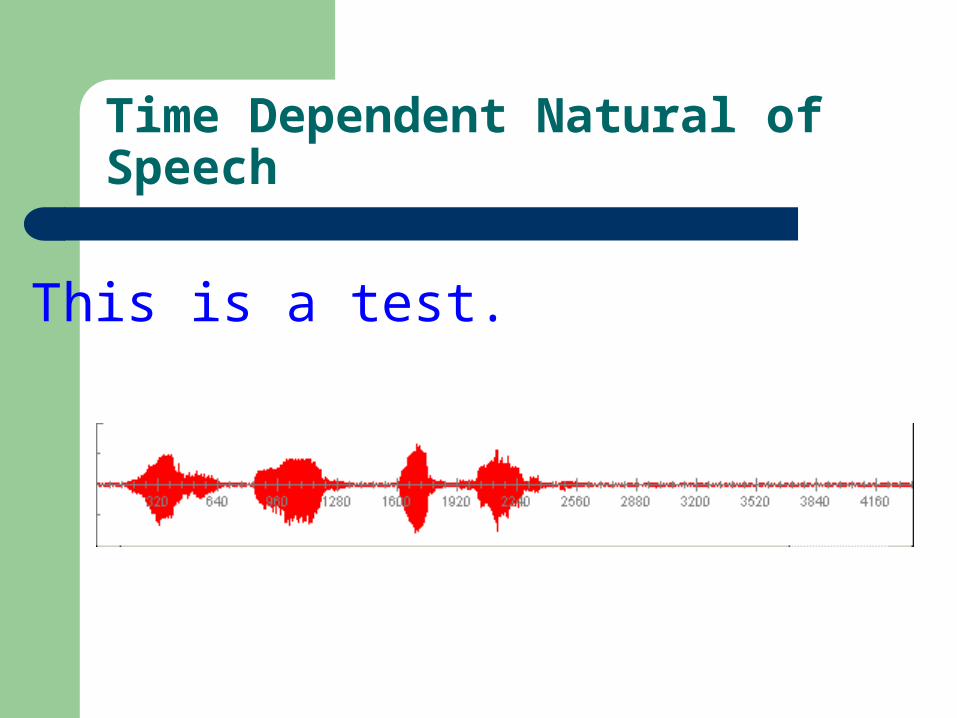
Time Dependent Natural of Speech
This is a test.
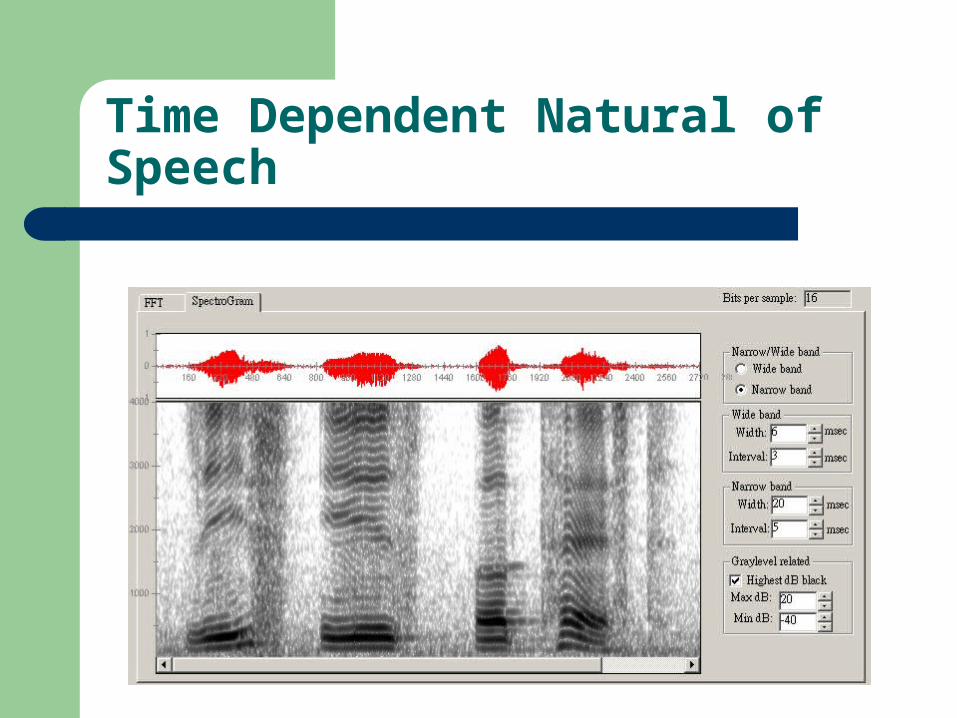
Time Dependent Natural of Speech
Short-Time Behavior of Speech
Assumption– The properties of speech signal change
slowly with time.
Analysis Frames– Short segment of speech signal.– Overlap one another usually.
Time-Dependent Analyses
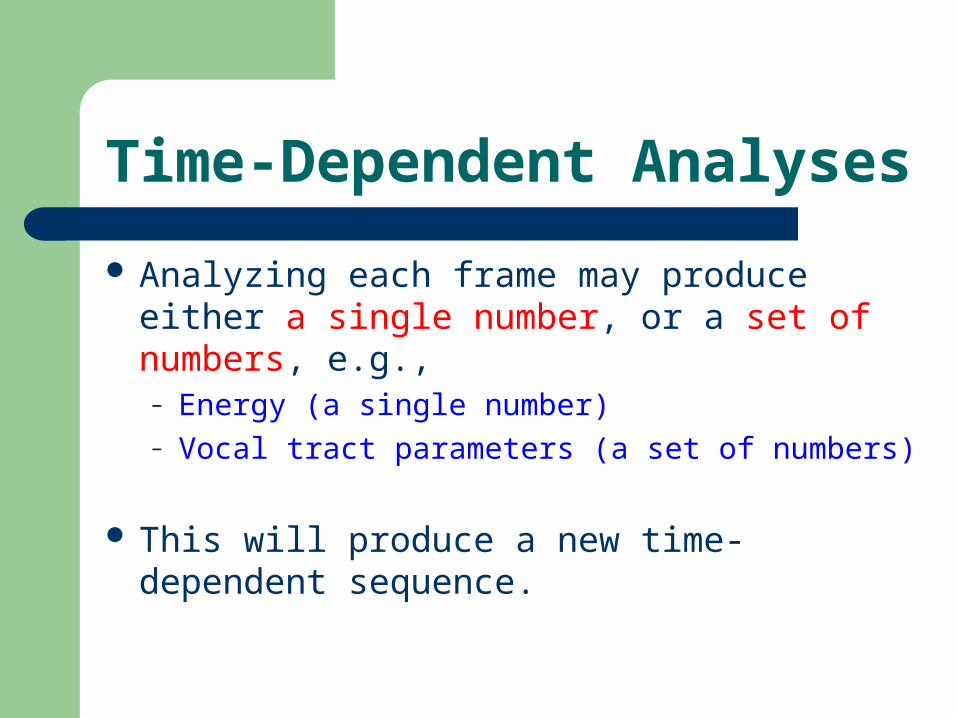
Analyzing each frame may produce either a single number, or a set of numbers, e.g.,– Energy (a single number)– Vocal tract parameters (a set of numbers)
This will produce a new time-dependent sequence.
General Form
m
n mnwmxTQ )()]([
m
n mnwmxTQ )()]([
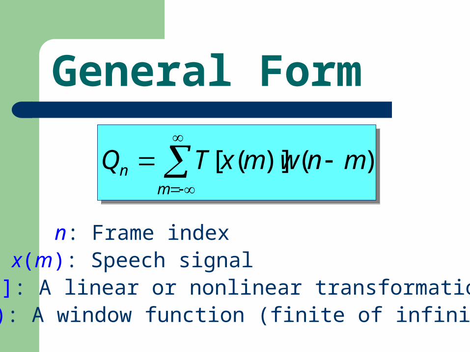
n: Frame indexx(m): Speech signalT[ ]: A linear or nonlinear transformation.
w(m): A window function (finite of infinite).
General Form
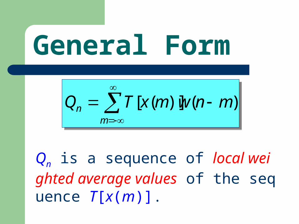
Qn is a sequence of local weighted average values of the sequence T[x(m)].
m
n mnwmxTQ )()]([
m
n mnwmxTQ )()]([
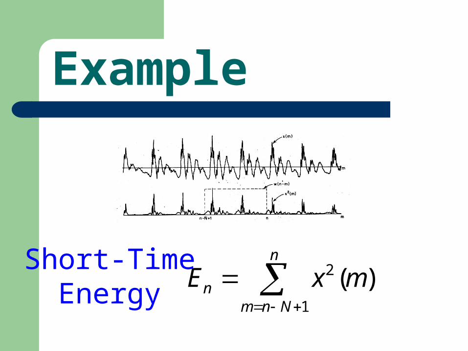
Example
m
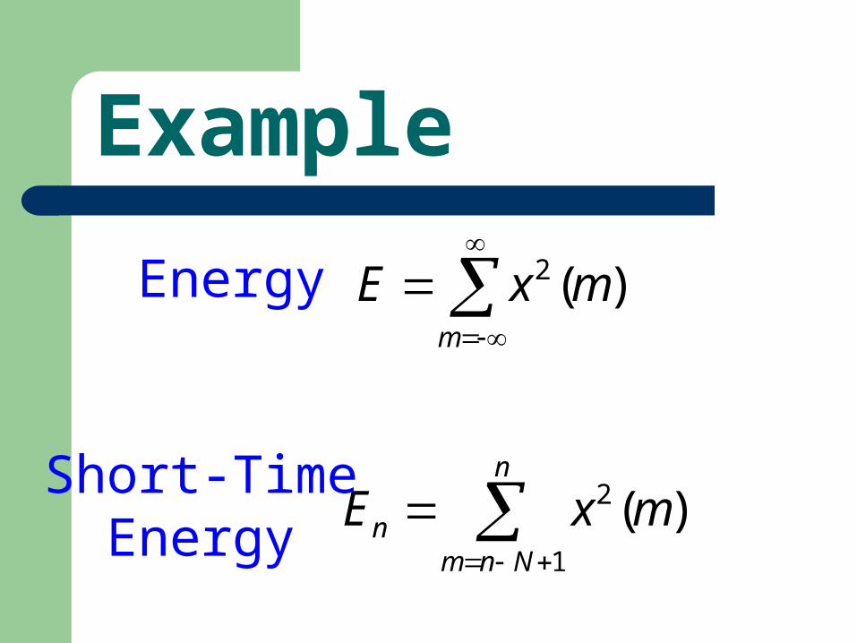
mxE )(2Energy
2
1
( )n
nm n N
E x m
Short-TimeEnergy
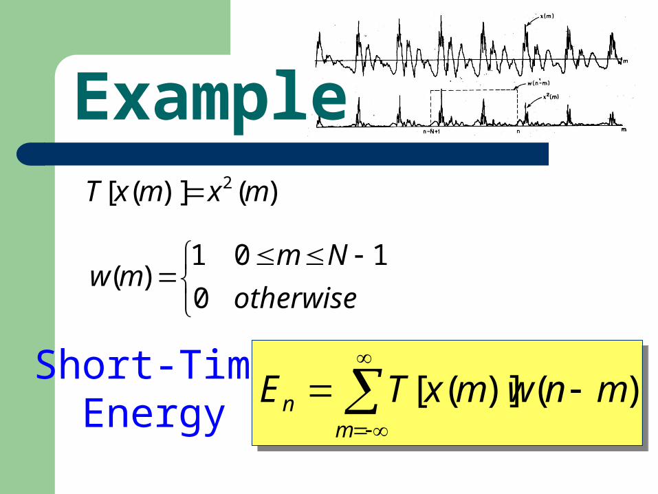
Example
2
1
( )n
nm n N
E x m
Short-TimeEnergy
2
1
( )n
nm n N
E x m
Short-TimeEnergy
)()]([ 2 mxmxT
otherwise
Nmmw
0
101)(
m
n mnwmxTE )()]([
m
n mnwmxTE )()]([
Example
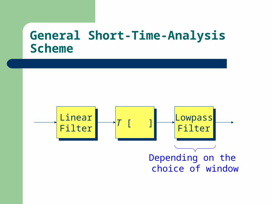
General Short-Time-Analysis Scheme
T [ ]T [ ]LinearFilter
LinearFilter
LowpassFilter
LowpassFilter
Depending on the choice of window
Time-Domain Methods for Speech Processing
Short-Time Energy and Average Magnitude
Applications
Silence Detection
Segmentation
Lip Sync
…
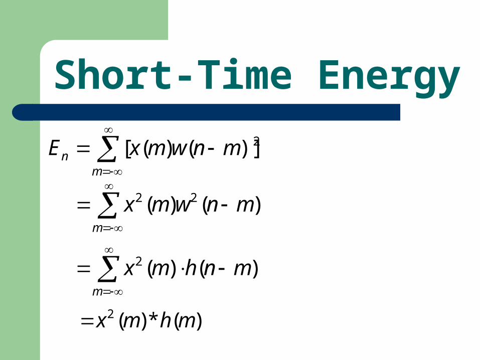
Short-Time Energy
m
n mnwmxE 2)]()([
m
mnwmx )()( 22
m
mnhmx )()(2
)(*)(2 mhmx
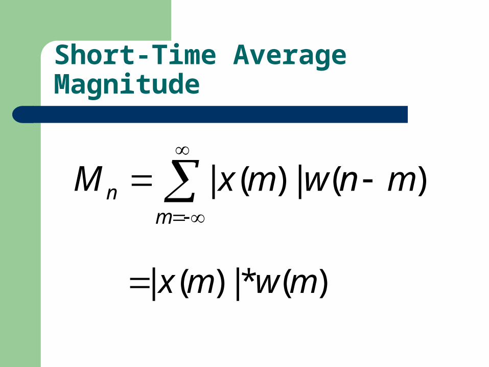
Short-Time Average Magnitude
m
n mnwmxM )(|)(|
)(*|)(| mwmx
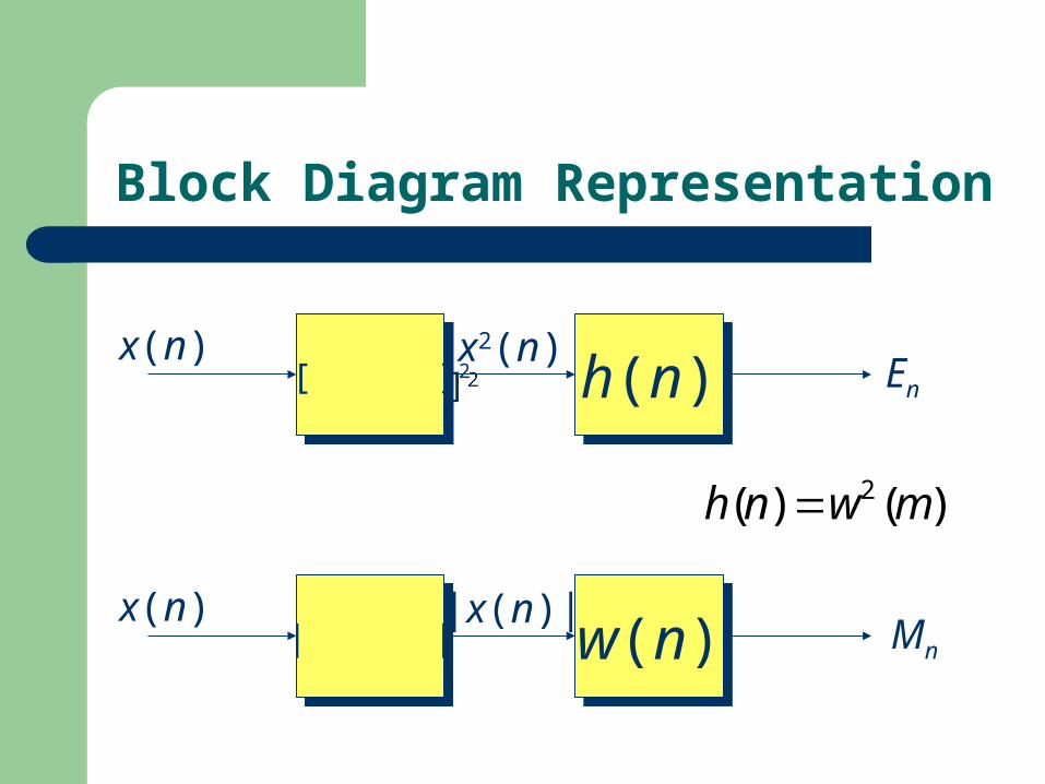
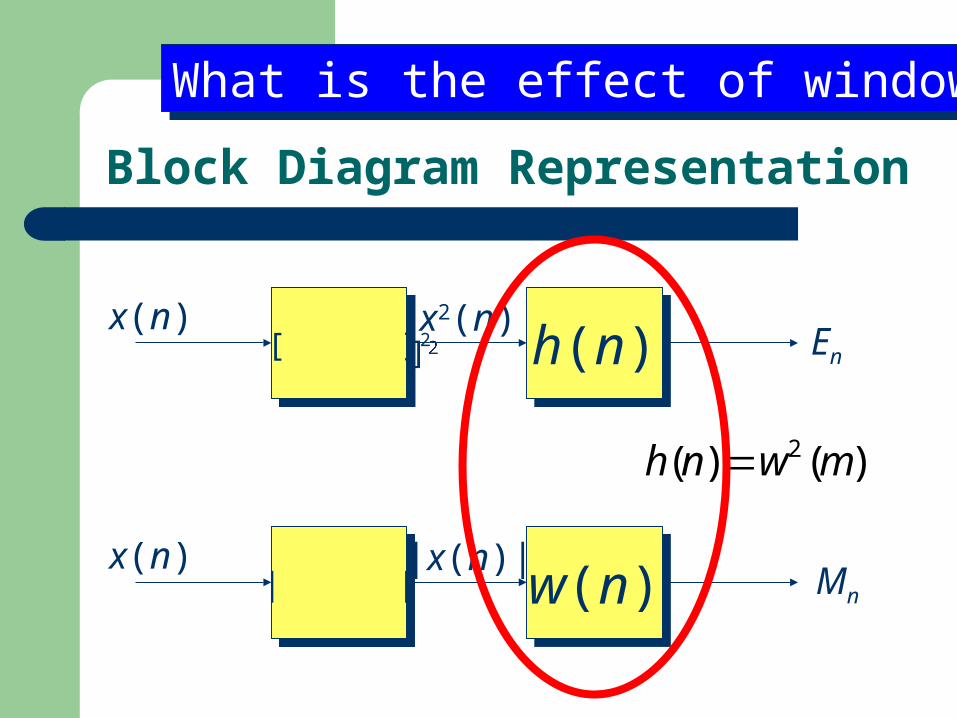
Block Diagram Representation
[ ]2 [ ]2x(n) x2(n)
| || |x(n) |x(n)|
h(n)h(n) En
w(n)w(n) Mn
)()( 2 mwnh
Block Diagram Representation
[ ]2 [ ]2x(n) x2(n)
| || |x(n) |x(n)|
h(n)h(n) En
w(n)w(n) Mn
)()( 2 mwnh
What is the effect of windows?What is the effect of windows?
The Effects of Windows
Window length
Window function
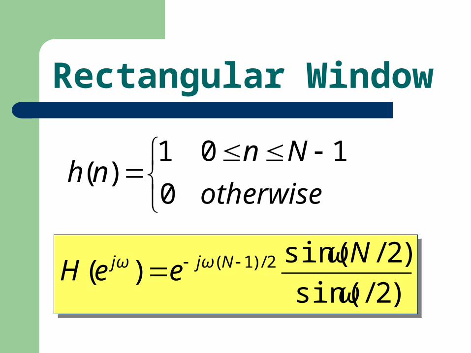
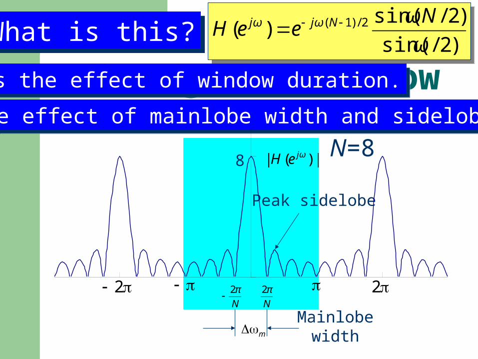
Rectangular Window
otherwise
Nnnh
0
101)(
)2/sin(
)2/sin()( 2/)1(
ω
ωNeeH Njωjω
)2/sin(
)2/sin()( 2/)1(
ω
ωNeeH Njωjω
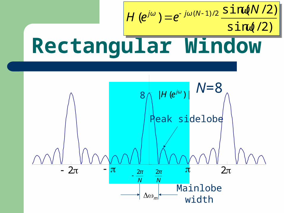
mMainlobe
width
Rectangular Window)2/sin(
)2/sin()( 2/)1(
ω
ωNeeH Njωjω
)2/sin(
)2/sin()( 2/)1(
ω
ωNeeH Njωjω
Peak sidelobe
2 2
|)(| jωeH
N
π2
N
π2
N=88
Rectangular Window)2/sin(
)2/sin()( 2/)1(
ω
ωNeeH Njωjω
)2/sin(
)2/sin()( 2/)1(
ω
ωNeeH Njωjω What is this?What is this?
Discuss the effect of window duration.Discuss the effect of window duration.
Discuss the effect of mainlobe width and sidelobe peak.Discuss the effect of mainlobe width and sidelobe peak.
mMainlobe
width
Peak sidelobe
2 2
|)(| jωeH
N
π2
N
π2
N=88
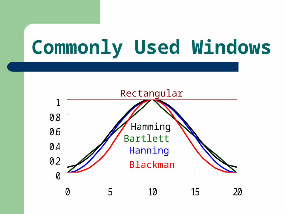
Commonly Used Windows
0
0.20.4
0.60.8
1
0 5 10 15 20
Rectangular
Blackman
HanningBartlettHamming
0
0.20.4
0.60.8
1
0 5 10 15 20
Rectangular
Blackman
HanningBartlettHamming
0
0.20.4
0.60.8
1
0 5 10 15 20
Rectangular
Blackman
HanningBartlettHamming
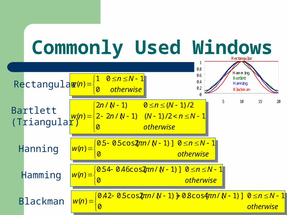
Commonly Used Windows
otherwise
Nnnw
0
101)(
otherwise
Nnnw
0
101)(
otherwise
NnNNn
NnNn
nw
0
12/)1()1/(22
2/)1(0)1/(2
)(
otherwise
NnNNn
NnNn
nw
0
12/)1()1/(22
2/)1(0)1/(2
)(
otherwise
NnNπnnw
0
10)]1/(2cos[5.05.0)(
otherwise
NnNπnnw
0
10)]1/(2cos[5.05.0)(
otherwise
NnNπnnw
0
10)]1/(2cos[46.054.0)(
otherwise
NnNπnnw
0
10)]1/(2cos[46.054.0)(
otherwise
NnNπnNπnnw
0
10)]1/(4cos[8.0)]1/(2cos[5.042.0)(
otherwise
NnNπnNπnnw
0
10)]1/(4cos[8.0)]1/(2cos[5.042.0)(
Rectangular
Bartlett(Triangular)
Hanning
Hamming
Blackman
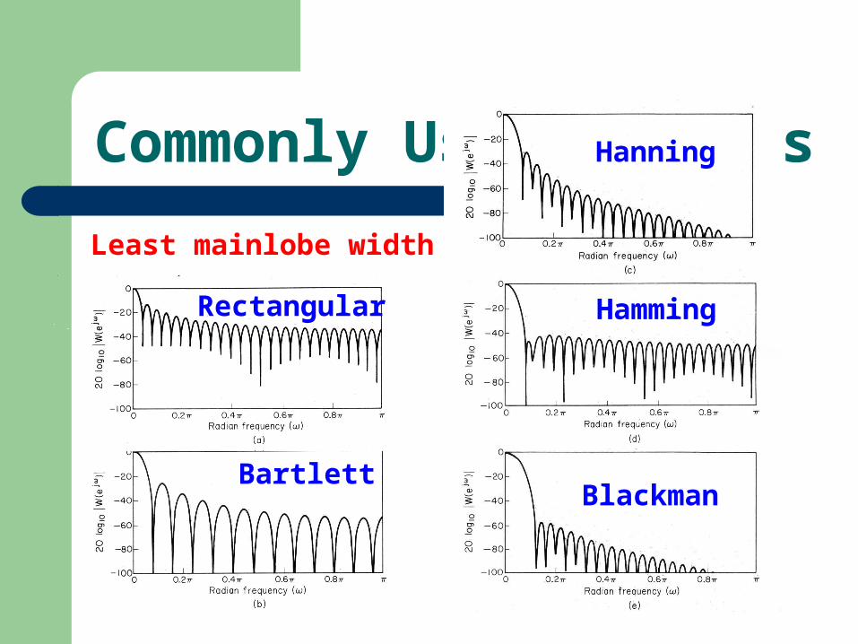
Commonly Used Windows
Rectangular
Bartlett
Hanning
Hamming
Blackman
Least mainlobe width
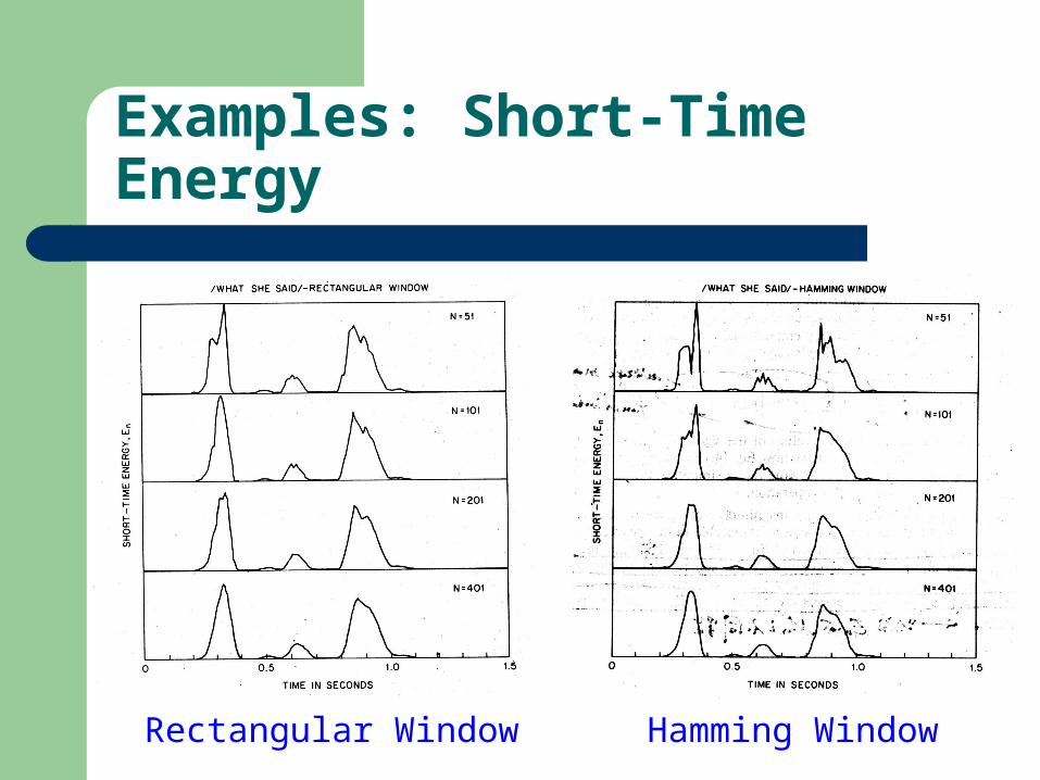
Examples: Short-Time Energy
Rectangular Window Hamming Window
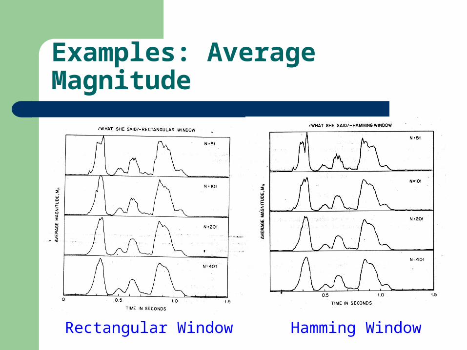
Examples: Average Magnitude
Rectangular Window Hamming Window
The Effects of Window Length
Increasing the window length N, decreases the bandwidth.
If N is too small, e.g., less than one pitch period, En and Mn will fluctuate very rapidly.
If N is too large, e.g., on the order of several pitch periods, En and Mn will change very slowly.
The Choice of Window Length
No signal value of N is entirely satisfactory.
This is because the duration of a pitch period varies from about 2 ms for a high pitch female or a child, up to 25 ms for a very low pitch male.
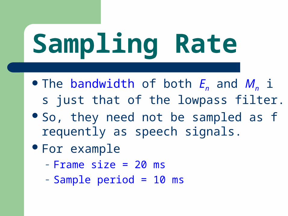
Sampling RateThe bandwidth of both En and Mn is just that
of the lowpass filter.So, they need not be sampled as frequently as
speech signals.For example
– Frame size = 20 ms– Sample period = 10 ms
Main Applications of En and Mn
To provide the basis for distinguishing voiced speech segments from unvoiced segments.
Silence detection.

Differences of En and Mn
m
n mnwmxE 2)]()([
m
n mnwmxE 2)]()([
m
n mnwmxM )(|)(|
m
n mnwmxM )(|)(|
Emphasizing large sample-to-sample variations in x(n).
The dynamic range (max/min) is approximately the square root of En.
The differences in level between voiced and unvoiced regions are not as pronounced as En.
FIR and IIR
All the windows that we discussed are FIR’s.
Each of them is a lowpass filter.
It can also be an IIR.
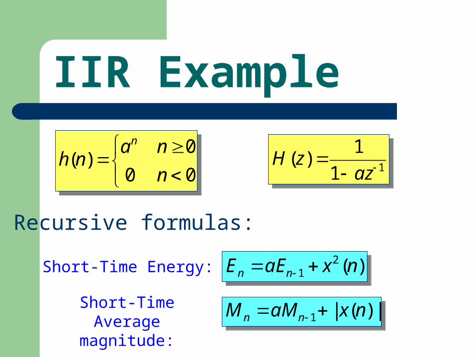
IIR Example
00
0)(
n
nanh
n
00
0)(
n
nanh
n
11
1)(
azzH 11
1)(
azzH
Recursive formulas:
)(21 nxaEE nn
)(21 nxaEE nn
|)(|1 nxaMM nn |)(|1 nxaMM nn
Short-Time Energy:
Short-TimeAverage magnitude:

Time-Domain Methods for Speech Processing
Short-Time Average
Zero-Crossing Rate
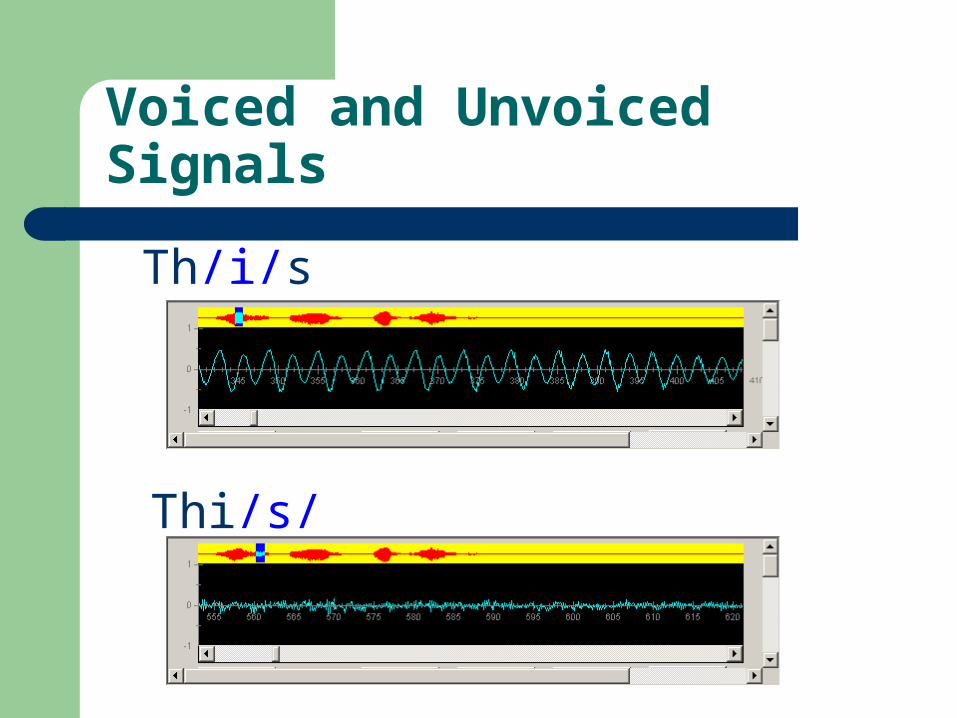
Voiced and Unvoiced Signals
Th/i/s
Thi/s/
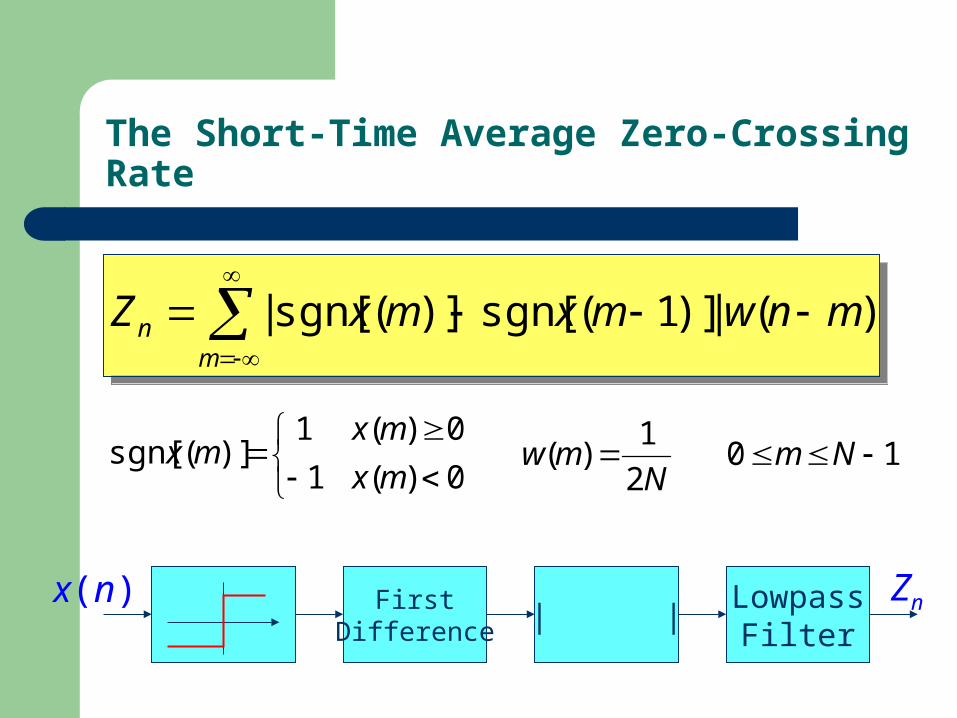
The Short-Time Average Zero-Crossing Rate
m
n mnwmxmxZ )(|)]1(sgn[)](sgn[|
m
n mnwmxmxZ )(|)]1(sgn[)](sgn[|
x(n) FirstDifference | |
ZnLowpassFilter
0)(1
0)(1)](sgn[
mx
mxmx 10
2
1)( Nm
Nmw
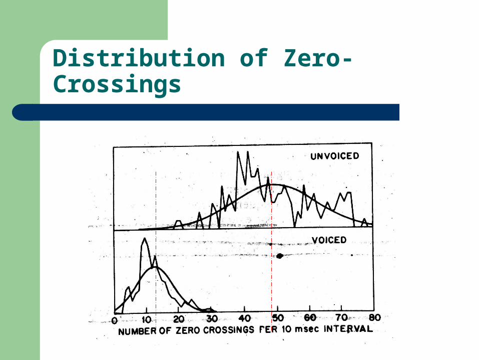
Distribution of Zero-Crossings
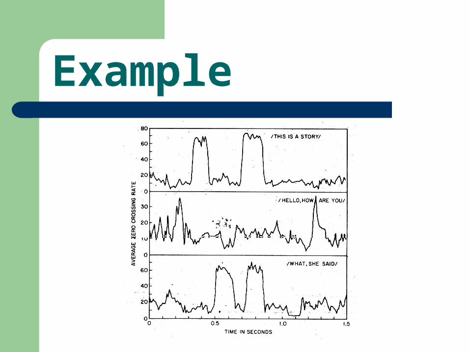
Example
Time-Domain Methods for Speech Processing
Speech vs. Silence Discrimination Using
Energy and Zero-Crossing
Speech vs. Silence Discrimination
Locating the beginning and end of a speech
utterance in the environment with background
of noise.
Applications:– Segmentation of isolated word
– Automatic speech recognition
– Save bandwidth for speech transmission
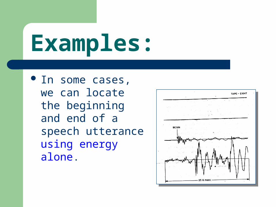
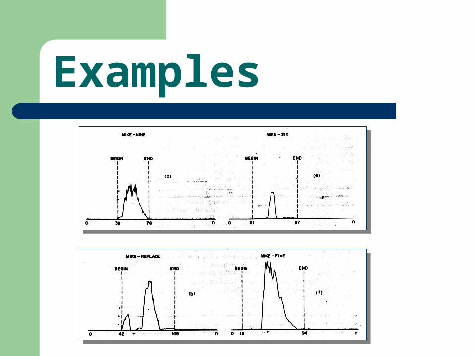
Examples: In some cases, we
can locate the beginning and end of a speech utterance using energy alone.
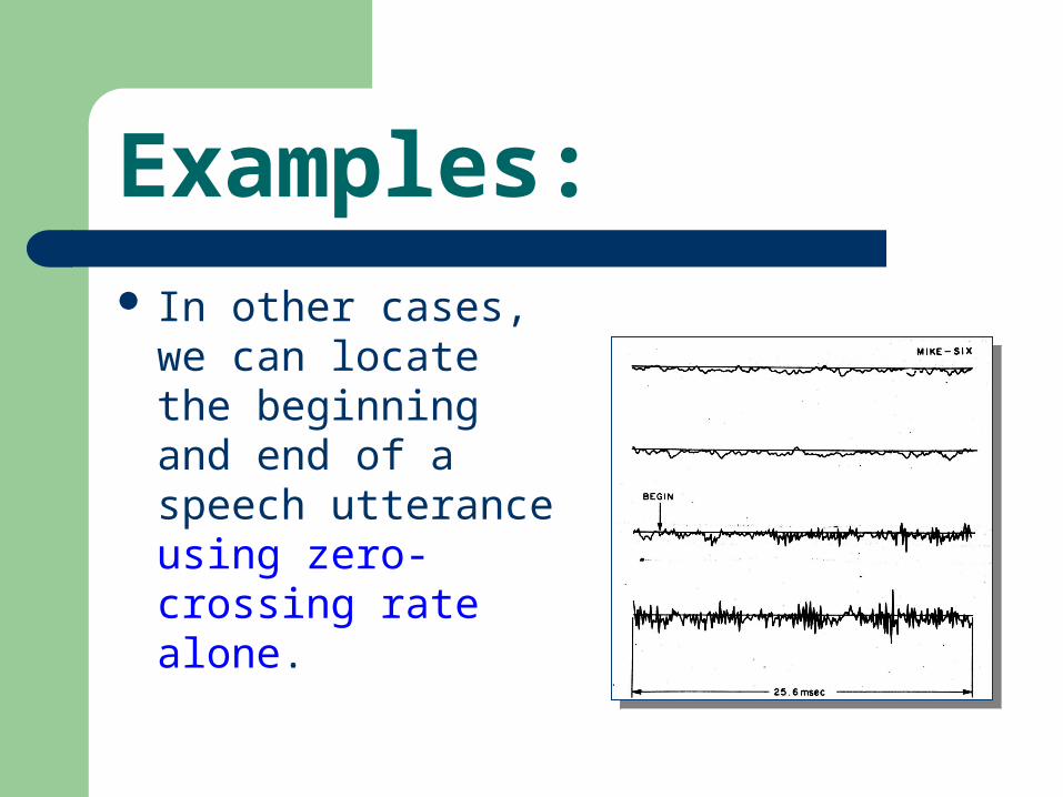
Examples: In other cases, we
can locate the beginning and end of a speech utterance using zero-crossing rate alone.
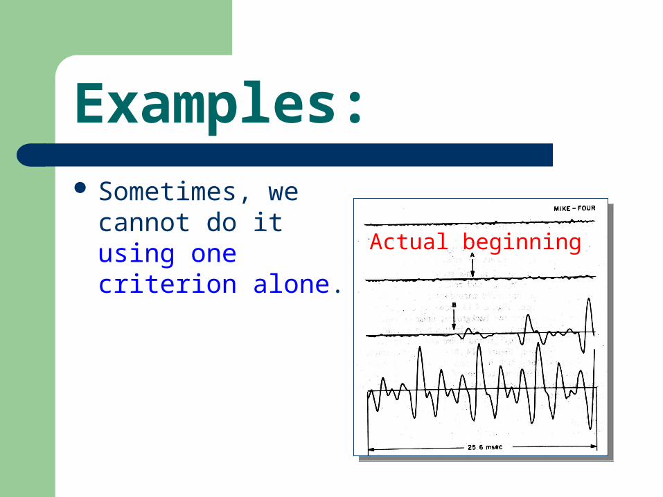
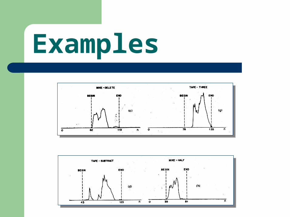
Examples: Sometimes, we
cannot do it using one criterion alone. Actual beginning
Difficulties In general, it is difficult to locate the boundaries
if we encounter the following cases:– Weak fricatives (/f/, /th/, /h/) at the beginning or end.– Weak plosive bursts (/p/, /t/, /k/) at the beginning or
end.– Nasals at the end.– Voiced fricatives which become devoiced at the end
of words.– Trailing off of vowel sounds at the end of an utteran
ce.
Rabiner and Sambur
10 msec frame with sampling rate 100 time/sec is used.
The algorithm assumes that the first 100 msec of the interval contains no speech.
The means and standard deviations of the average magnitude and zero-crossing rate of this interval are computed to characterize the background noise.
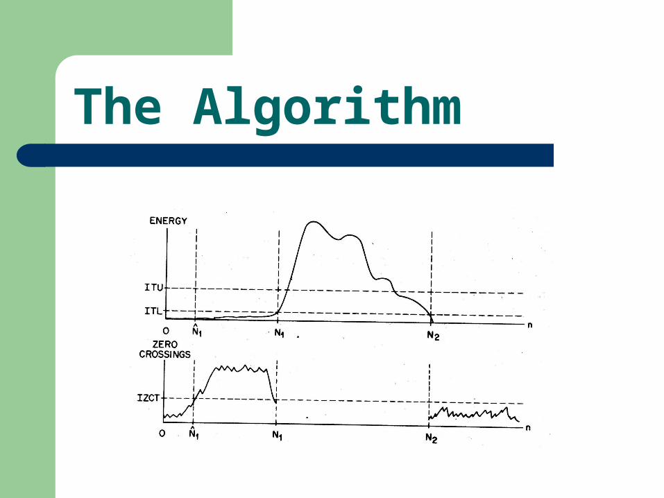
The Algorithm
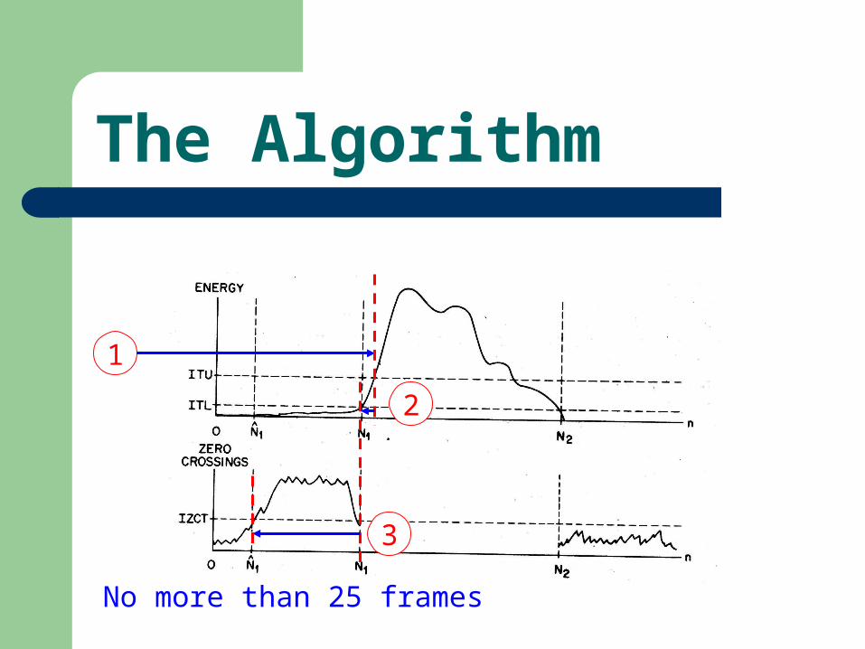
The Algorithm
1
2
3
No more than 25 frames
Examples
Examples
Time-Domain Methods for Speech Processing
The Short-Time
Autocorrelation Function
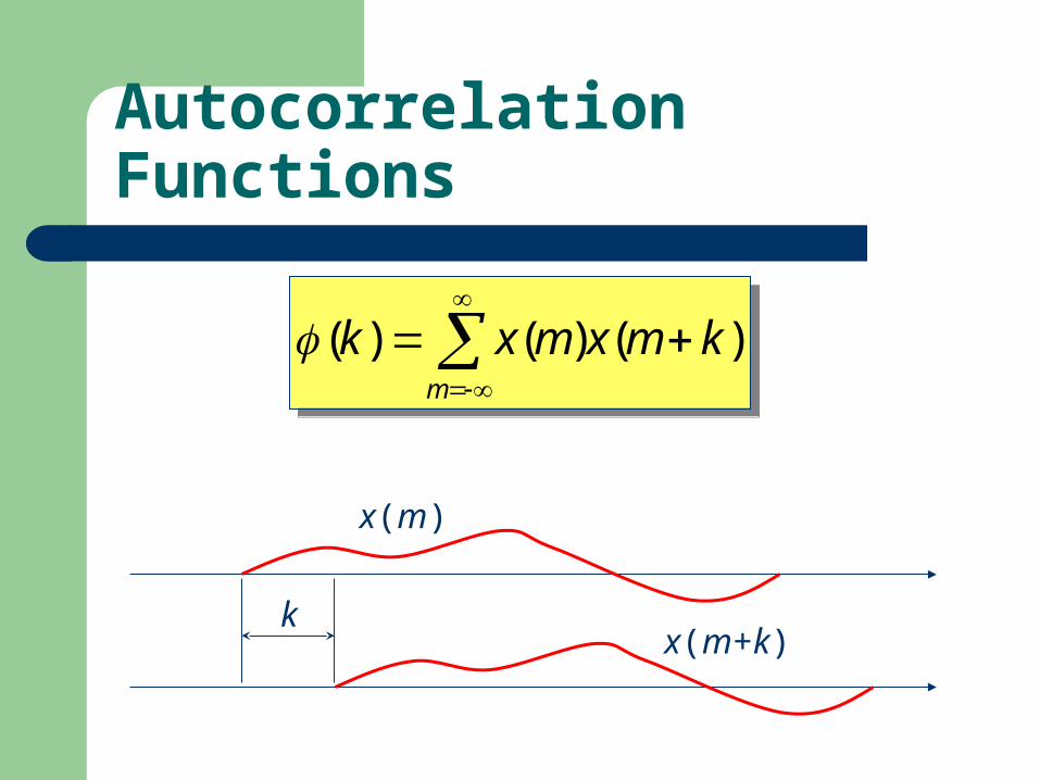
Autocorrelation Functions
m
kmxmxk )()()(
m
kmxmxk )()()(
x(m)
x(m+k)k
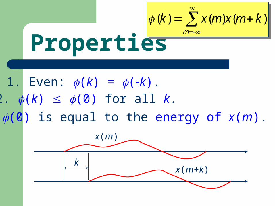
Properties
m
kmxmxk )()()(
m
kmxmxk )()()(
1. Even: (k) = (k).2. (k) (0) for all k.
3. (0) is equal to the energy of x(m).
x(m)
x(m+k)k
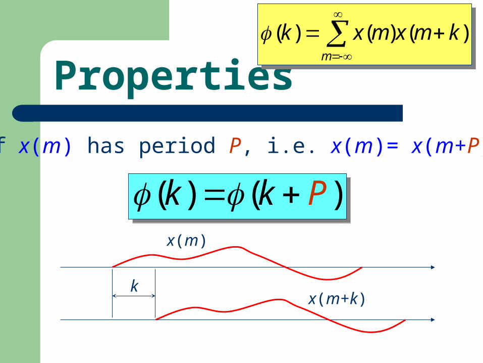
Properties
m
kmxmxk )()()(
m
kmxmxk )()()(
4. If x(m) has period P, i.e. x(m)= x(m+P), then
( ) ( )Pk k ( ) ( )Pk k x(m)
x(m+k)k
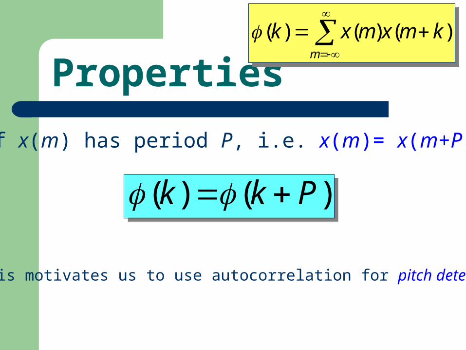
Properties
m
kmxmxk )()()(
m
kmxmxk )()()(
4. If x(m) has period P, i.e. x(m)= x(m+P), then
)()( Pkk )()( Pkk
This motivates us to use autocorrelation for pitch detection.
x(m+k)w(nkm)
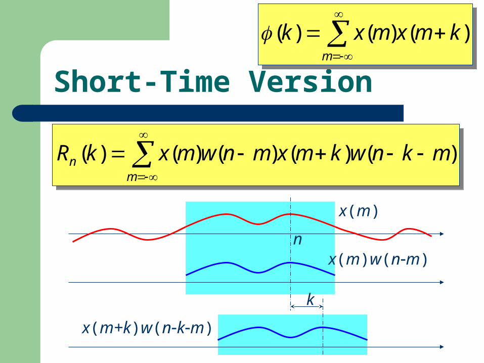
Short-Time Version
m
kmxmxk )()()(
m
kmxmxk )()()(
m
n mknwkmxmnwmxkR )()()()()(
m
n mknwkmxmnwmxkR )()()()()(
x(m)
x(m)w(nm)n
k
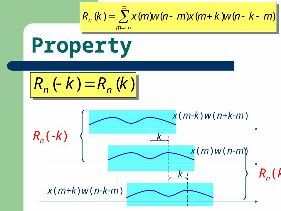
Property
m
n mknwkmxmnwmxkR )()()()()(
m
n mknwkmxmnwmxkR )()()()()(
)()( kRkR nn )()( kRkR nn
x(mk)w(n+km)
k
x(m)w(nm)
x(m+k)w(nkm)
k Rn(k)
Rn(k)
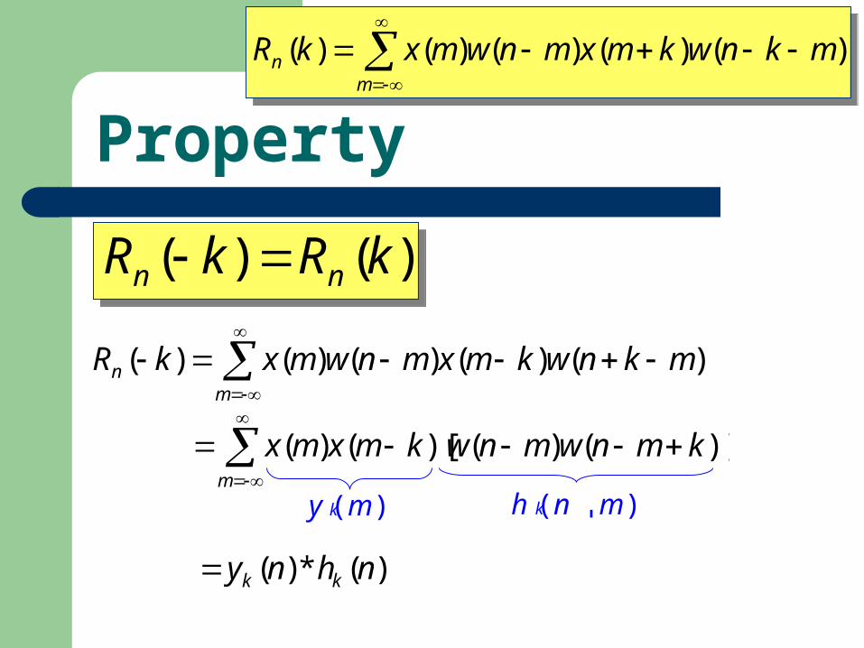
Property
m
n mknwkmxmnwmxkR )()()()()(
m
n mknwkmxmnwmxkR )()()()()(
)()( kRkR nn )()( kRkR nn
m
n mknwkmxmnwmxkR )()()()()(
m
kmnwmnwkmxmx )]()()[()(
y k(m) h k(n m)
)(*)( nhny kk
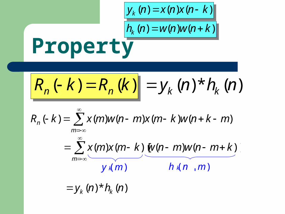
Property
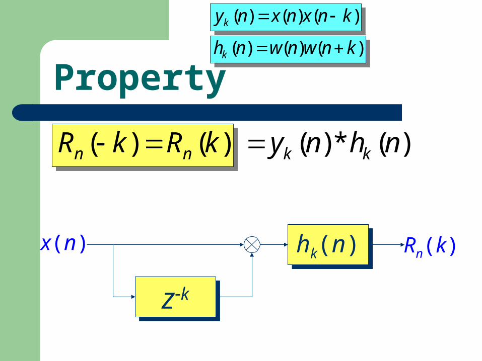
)()()( knxnxnyk )()()( knxnxnyk
)()( kRkR nn )()( kRkR nn
m
n mknwkmxmnwmxkR )()()()()(
m
kmnwmnwkmxmx )]()()[()(
y k(m) h k(n m)
)(*)( nhny kk
)()()( knwnwnhk )()()( knwnwnhk
)(*)( nhny kk
Property
)()( kRkR nn )()( kRkR nn )(*)( nhny kk
zkzk
hk(n)hk(n)x(n) Rn(k)
)()()( knxnxnyk )()()( knxnxnyk
)()()( knwnwnhk )()()( knwnwnhk
Another Formulation
m
n mknwkmxmnwmxkR )()()()()(
m
n mknwkmxmnwmxkR )()()()()(
m
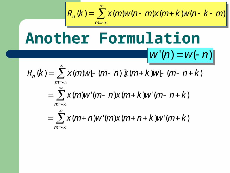
n knmwkmxnmwmxkR )]([)()]([)()(
m
knmwkmxnmwmx )(')()(')(
)()(' nwnw )()(' nwnw
m
kmwknmxmwnmx )(')()(')(
Another Formulation
m
n knmwkmxnmwmxkR )]([)()]([)()(
m
knmwkmxnmwmx )(')()(')(
)()(' nwnw )()(' nwnw
m
kmwknmxmwnmx )(')()(')(
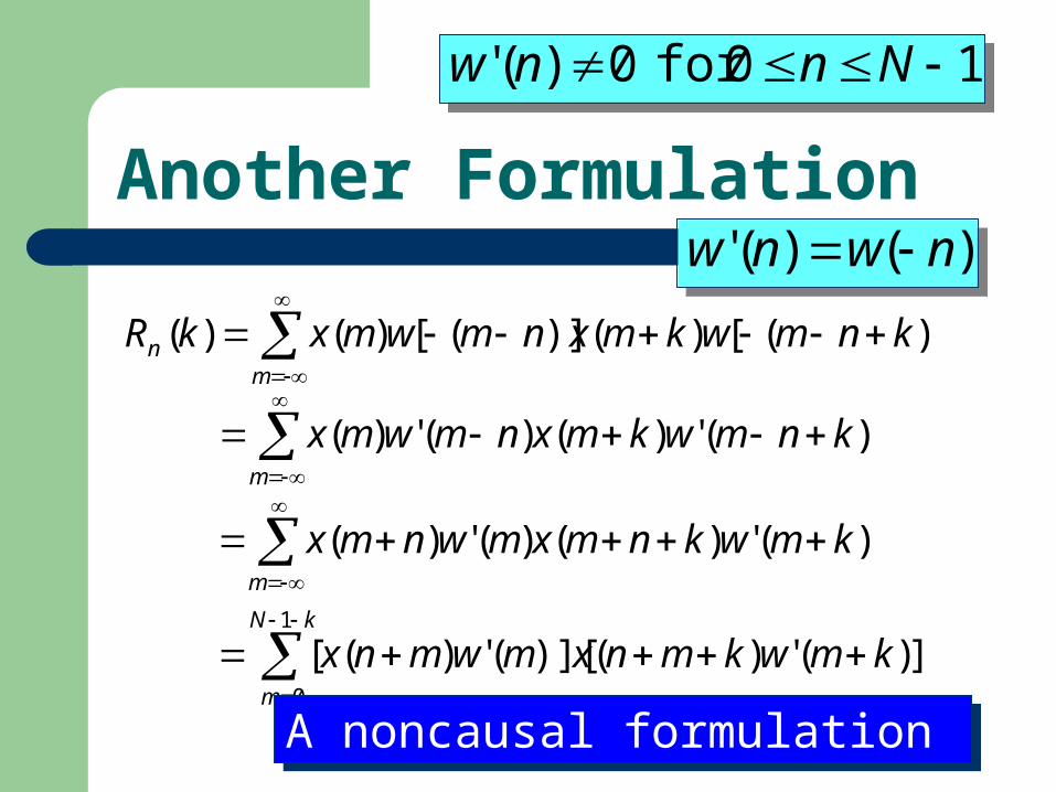
10for 0)(' Nnnw 10for 0)(' Nnnw
])(')()][(')([1
0
kN
m
kmwkmnxmwmnx
A noncausal formulation A noncausal formulation
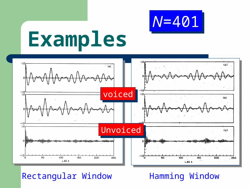
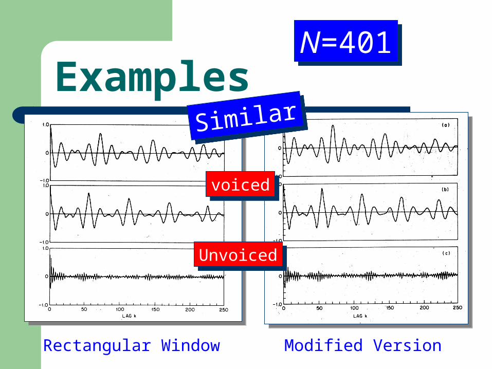
Examples
Rectangular Window Hamming Window
N=401N=401
voicedvoiced
UnvoicedUnvoiced
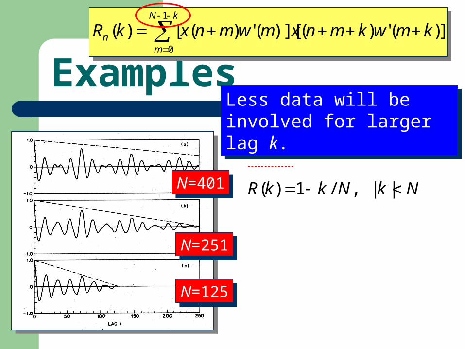
Examples])(')()][(')([)(
1
0
kN
mn kmwkmnxmwmnxkR ])(')()][(')([)(
1
0
kN
mn kmwkmnxmwmnxkR
Less data will be involved for larger lag k.
Less data will be involved for larger lag k.
NkNkkR || ,/1)(N=401N=401
N=251N=251
N=125N=125
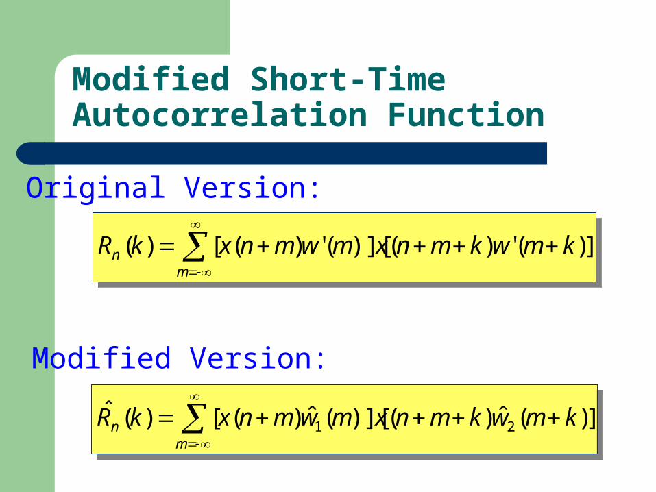
Modified Short-Time Autocorrelation Function
])(')()][(')([)(
m
n kmwkmnxmwmnxkR ])(')()][(')([)(
m
n kmwkmnxmwmnxkR
Original Version:
])(ˆ)()][(ˆ)([)(ˆ21
m
n kmwkmnxmwmnxkR ])(ˆ)()][(ˆ)([)(ˆ21
m
n kmwkmnxmwmnxkR
Modified Version:
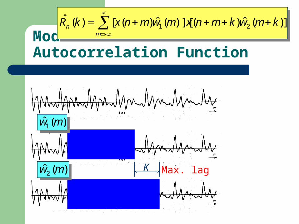
Modified Short-Time Autocorrelation Function
])(ˆ)()][(ˆ)([)(ˆ21
m
n kmwkmnxmwmnxkR ])(ˆ)()][(ˆ)([)(ˆ21
m
n kmwkmnxmwmnxkR
K
)(ˆ1 mw )(ˆ1 mw
)(ˆ 2 mw )(ˆ 2 mw Max. lag
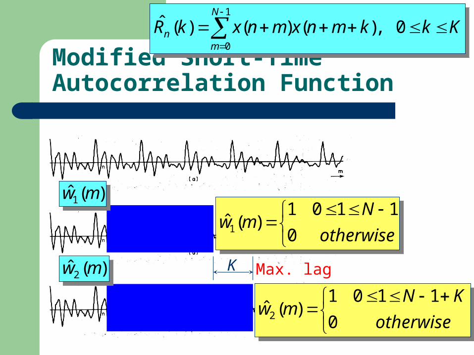
Modified Short-Time Autocorrelation Function
K
)(ˆ1 mw )(ˆ1 mw
)(ˆ 2 mw )(ˆ 2 mw Max. lag
otherwise
Nmw
0
1101)(ˆ1
otherwise
Nmw
0
1101)(ˆ1
otherwise
KNmw
0
1101)(ˆ 2
otherwise
KNmw
0
1101)(ˆ 2
KkkmnxmnxkRN
mn
0 ,)()()(ˆ1
0
KkkmnxmnxkRN
mn
0 ,)()()(ˆ1
0
Examples
Rectangular Window
N=401N=401
voicedvoiced
UnvoicedUnvoiced
Modified Version
SimilarSimilar
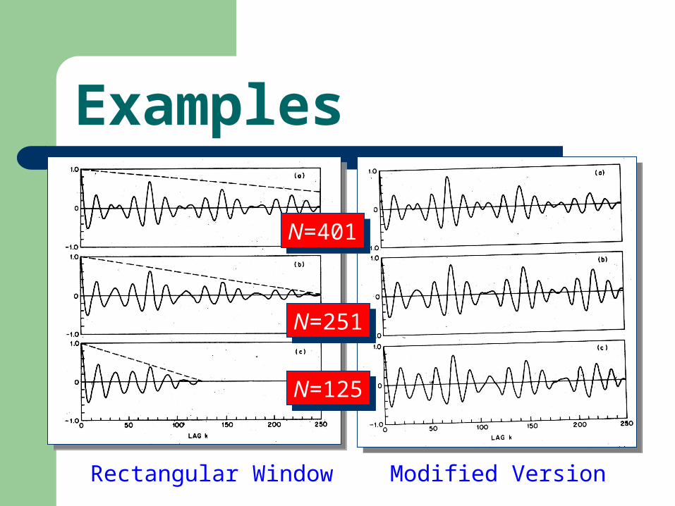
Examples
Rectangular Window Modified Version
N=401N=401
N=251N=251
N=125N=125

Time-Domain Methods for Speech Processing
The Short-Time
Average Magnitude
Difference Function
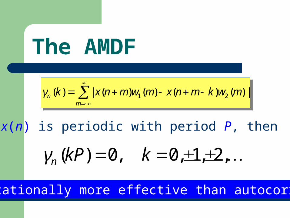
The AMDF
m
n mwkmnxmwmnxkγ |)()()()(|)( 21
m
n mwkmnxmwmnxkγ |)()()()(|)( 21
If x(n) is periodic with period P, then
,2,1,0 ,0)( kkPγn
Computationally more effective than autocorrelation.Computationally more effective than autocorrelation.
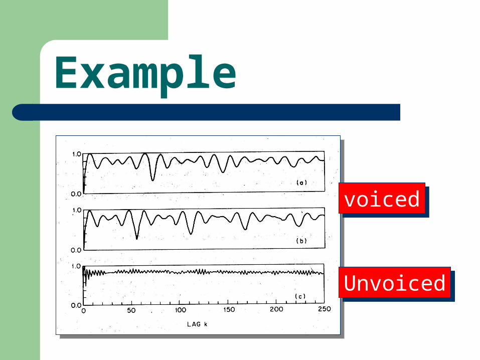
Example
voicedvoiced
UnvoicedUnvoiced

Exercise Recording a piece of yours speech to perform
voice/unvoice segmentation.
Design a effective algorithm to perform autocorrelation.