635

2015,27(5):635-646 DOI: 10.1016/S1001-6058(15)60526-1

Time domain simulations of radiation and diffraction by a Rankine panel me- thod* ZHANG Wei (张伟)1, ZOU Zaojian (邹早建)1,2 1. School of Naval Architecture, Ocean and Civil Engineering, Shanghai Jiao Tong University, Shanghai 200240, China, E-mail: drwood@sjtu.edu.cn 2. State Key Laboratory of Ocean Engineering, Shanghai Jiao Tong University, Shanghai 200240, China (Received April 3, 2014, Revised August 16, 2014) Abstract: The radiation and the diffraction of a ship with a forward speed are studied by using a time domain Rankine panel method. The free surface conditions are linearized onto an undisturbed free surface based on the double body flow. The linearized body boundary condition is applied on the mean wetted hull surface. The fluid domain boundary is discretized by a collection of quadric panels. The unknown quantities, including the free surface elevation, the normal flux over the free surface and the potential on the fluid domain boundary, are determined at each time step. The numerical results are compared with experimental data and other numerical solutions, showing satisfactory agreements. Key words: radiation, diffraction, Rankine source, panel method, time domain analysis

Introduction In the past two decades, the three-dimensional

panel method combined with the time domain analysis techniques finds increasingly wider applications in si- mulating the free surface flow around a ship. Based on the choices of the elementary singularity, there are two general categories of the time domain panel me- thods for the ship hydrodynamics studies.

The first category employs the transient Green function. The methods of this category have the ad- vantages of the free surface integration being avoided and the radiation condition satisfied automatically. But the integration of the transient Green function is made difficult, especially when the ship is not wall- sided. Recent progresses in this area were reported, such as Datta and Sen[1], Duan and Dai[2], Zhu et al.[3].

The second category of the methods uses the

* Project supported by the National Natural Science Foun- dation of China (Grant No. 51279106). Biography: ZHANG Wei (1983-), Male, Ph. D. Candidate Corresponding author: ZOU Zao-jian, E-mail: zjzou@sjtu.edu.cn

Rankine source as the elementary singularity. Since the Rankine source satisfies only the far field decay condition, the singularities must be distributed on both the body surface and a part of the free surface. A nu- merical scheme is also needed to treat the temporal discretization. However, the advantage of the Rankine panel methods (RPM) is twofold: the Rankine source is simple to evaluate, and the distribution of the panels over the free surface provides a great deal of flexibili- ty for different kinds of free surface boundary condi- tions. Nakos et al.[4] presented their numerical solutio- ns of the linear transient wave-body interaction pro- blems, using the RPM with a neutrally stable time dis- cretization scheme. Their work was extended to the nonlinear cases by Huang [5]. The same discretization scheme was also used by Kim et al.[6]. Zhang et al.[7] conducted the time domain simulations of the radia- tion and diffraction forces by using the desingularized boundary integral methods and the mixed Euler- Lagrange time stepping technique. The wave-induced ship motions were also simulated using the time do- main RPM by other researchers, such as Yasukawa[8], He and Kashiwagi[9] and Chen and Zhu[10-12].

This study carries out the numerical simulation of the radiation and the diffraction of a ship with a for- ward speed, using a time domain Rankine panel me- thod. The free surface conditions are linearized onto

636

the undisturbed free surface based on the double body flow. The linearized body boundary condition is app- lied on the mean wetted hull surface. The discretiza- tion algorithms are based on the work of Nakos et al.[4]. However, different from their original method, the present study uses a collection of quadric panels instead of the plane quadrilateral panels to discretize the fluid domain boundary. Such modification is to enhance the geometrical continuity between panels, and subsequently increase the accuracy of the numeri- cal results. Simulations of the radiation and diffraction waves are carried out for the Wigley I hull and the S- 175 container ship. The numerical results of the hy- drodynamic coefficients and the wave-exciting forces are compared with experimental data and other nume- rical solutions to verify the effectiveness of the prese- nt numerical method. 1. Mathematical formulation

The ship is assumed rigid and traveling at a speed

0= ( ,0,0)UU in regular waves. The water depth is

assumed to be infinite. A ship-fixed right-handed coo- rdinate system -O xyz is used. The positive x is to-

wards the bow and the positive z points upward. The xy plane is coincident with the calm water level and

the origin is at the midship. Under the assumption that the fluid is inviscid

and incompressible, and the flow is irrotational, the fluid velocity potential can be introduced, to esta- blish the following boundary value problem:

2 = 0 in fluid domain (1)

+ [ ( , , )] = 0z x y tt

on = ( , , )z x y t

(2)

2+ = + 0.5 + 0.5g Ut

on

= ( , , )z x y t (3)

( , )= +

t

n t

x

U n n

on body surface (4)

where n is the inward unit normal vector on the hull surface (out of fluid), is the oscillatory displaceme- nt of the hull surface, ( , , )x y t is the free surface ele-

vation and g is the gravitational acceleration.

To linearize the free surface boundary conditions (2) and (3), the total potential is decomposed into a double-body basis flow ( )D x and a perturbation

flow ( , )t x ,

( , ) = ( ) + ( , )Dt t x x x (5)

The double body flow is assumed to be the main

component of the order of (1)O . It can be expressed

as 0= +D U x , and satisfies the following

boundary conditions

=n

U n on BS (6a)

= 0z

on = 0z (6b)

where BS is the mean wetted hull surface.

The perturbation potential and the free surface

elevation are assumed small and are of the order of

( )O . By substituting Eq.(5) into Eq.(2) and Eq.(3), keeping the leading-order terms and neglecting the terms higher than ( )O , the linearized free surface

conditions can be obtained as follows:

2

2( ) = +

t z z

U on = 0z (7)

1

( ) = +2

gt

U U

on = 0z (8)

The perturbation flow ( , )t x and the wave ele-

vation are further decomposed as:

( , ) = ( , ) + ( , ) + ( , )d r It t t t x x x x (9)

( , , ) = ( , , ) + ( , , ) + ( , , )d r Ix y t x y t x y t x y t (10)

where ( , )I t x is the incident wave potential and

( , , )I x y t is the incident wave elevation. ( , )r t x and

( , )d t x stand for the radiation and diffraction pote-

ntials, respectively. ( , , )r x y t and ( , , )d x y t are the

radiation and diffraction wave elevations, respective- ly.

To evaluate the diffraction, the ship is assumed to advance in regular waves, but without any oscillation. The incident wave potential of unit amplitude in deep water is

0

( , ) = Re i exp[ ( i cos i sin )i ]I

gt k z x y t

x

(11)

637

where 0 is the frequency of the incident wave, k is

the wave number, 20= /k g for deep water, is

the angle between the phase velocity of the incident wave and the ship velocity, = for the head sea,

and is the encounter frequency defined as

20

0 0= cosUg

(12)

The boundary value problem for the diffraction

potential ( , )d t x is summarized as follows:

2 = 0d in fluid domain (13a)

2

2( ) = + d

d dt z z

U

( ) It

U on = 0z (13b)

( ) = ( )d It t

U U

( + )d Ig on = 0z (13c)

=d I

n n

on BS (13d)

For the radiation potential due to the unit ampli-

tude ship motion in the thi degree of freedom, the ship is given a forced harmonic oscillation

( ) = cosi t t , 0t (14)

where is the encounter frequency of interest.

The exact body boundary condition (4) is lineari- zed about the mean wetted body position following Newman[13]. Then the boundary value problem for the radiation potential ( , )r t x takes the form:

2 = 0r in fluid domain (15a)

2

2( ) = + r

r rt z z

U on = 0z

(15b)

( ) =r rgt

U on = 0z (15c)

6

=1

= +jrj j j

j

n mn t

on BS (15d)

where 1 2 3= ( , , )T is the rigid body translational

displacement, 4 5 6= ( , , )R is the rotational displa-

cement, 1 2 3( , , ) =n n n n , 4 5 6( , , ) =n n n x n , = ( ,xx

, )y z is the position vector and jm is the so-called

m-terms, which can be evaluated as follows:

1 2 3( , , ) = ( )( )m m m n U (16a)

4 5 6( , , ) = ( )[ ( )]m m m n x U (16b)

To complete the boundary value problems (13)

and (15), the far field boundary conditions are also ne- cessary for each unknown perturbation potential, to insure that the ship-generated wave propagates only outward. Additionally, the initial condition is

= = 0t

at = 0t (17)

Once the potential function is solved, the un-

steady pressure on the hull can be computed by using the linearized Bernoulli’s equation

= ( )pt

U (18)

and the unsteady hydrodynamic force 1 2 3= ( , , )F F FF

and the moment 4 5 6= ( , , )F F FM acting on the hull

can be determined as a generalized force

= dB

j jSF p n s , = 1, 2, , 6j (19)

2. Numerical implementation 2.1 Boundary integral equation

The fluid domain is bounded by the hull surface ( )BS , the undisturbed free surface ( )F and a control

surface at infinity ( )S . By applying the Green seco-

nd theorem, the Laplace equation can be put into the integral equation form as

( ) ( ) + ( ) ( , )dB

nF SC G

x x x x x x

( ) ( , )d = 0B

nF SG

x x x x (20)

638

where ( , )G x x is the Rankine source defined by

1 1

( , ) =4

G

x xx x

(21)

where ( )C x is the solid angle at the field point x and

the subscript n means the derivative along the outer normal of the fluid domain boundary. The contribu- tion of the control surface at infinity ( )S vanishes

owing to the decay of both ( , )G x x and ( , )t x as

x .

The integral Eq.(20) together with the correspo- nding linearized boundary conditions constitute a sys- tem of equations for the solutions with respect to the free surface elevation , the normal flux Z over

the free surface and the potential on the fluid do-

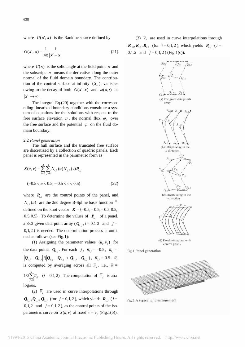
main boundary. 2.2 Panel generation

The hull surface and the truncated free surface are discretized by a collection of quadric panels. Each panel is represented in the parametric form as

2 2

, 2 ,2 ,=0 =0

( , ) = ( ) ( )i j i ji j

u v N u N vS P

( 0.5 0.5, 0.5 0.5)u v (22)

where ,i jP are the control points of the panel, and

, 2 ( )iN u are the 2nd degree B-Spline basis function [14]

defined on the knot vector = { 0.5, 0.5, 0.5,0.5, K

0.5,0.5} . To determine the values of ,i jP of a panel,

a 33 given data point array ( ,i jQ , = 0,1,2i and =j

0,1,2 ) is needed. The determination process is outli-

ned as follows (see Fig.1): (1) Assigning the parameter values ( , )i ju v for

the data points ,i jQ . For each j , 0 = 0.5ju ,

1 =ju

1, 0, 1, 0, 2, 1,/( )j j j j j j Q Q Q Q Q Q , 2 = 0.5ju . iu

is computed by averaging across all iju , i.e., =iu 2

=0

1/3 ijj

u ( = 0,1,2)i . The computation of jv is ana-

logous.

(2) jv are used in curve interpolations through

0, 1, 2,, ,j j jQ Q Q (for = 0,1,2j ), which yields ,i jR ( =i

0,1,2 and = 0,1,2j ), as the control points of the iso-

parametric curve on ( , )S u v at fixed = jv v (Fig.1(b)).

(3) jv

are used in curve interpolations through

,0 ,1 ,2, ,i i iR R R (for = 0,1,2i ), which yields ,i jP ( =i

0,1,2 and = 0,1,2j ) (Fig.1(c)).

Fig.1 Panel generation Fig.2 A typical grid arrangement

639

A typical arrangement of the whole grid, on both the free surface and the hull surface, is illustrated in Fig.2, in which the free surface grid extends 1.0L (ship length) in the transverse direction, 0.5L upst- ream and 1.0L downstream. The half ship is represe- nted by s sN M panels, while the panels on the free

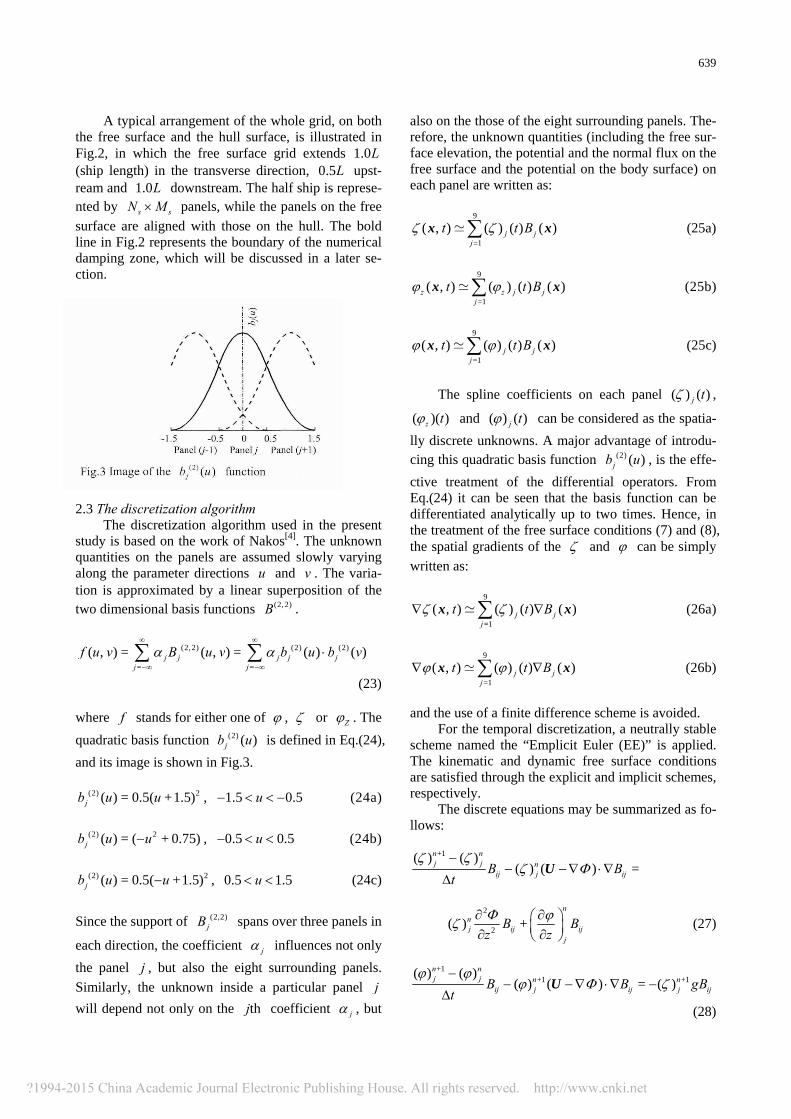
surface are aligned with those on the hull. The bold line in Fig.2 represents the boundary of the numerical damping zone, which will be discussed in a later se- ction. Fig.3 Image of the (2) ( )jb u function

2.3 The discretization algorithm

The discretization algorithm used in the present study is based on the work of Nakos[4]. The unknown quantities on the panels are assumed slowly varying along the parameter directions u and v . The varia- tion is approximated by a linear superposition of the two dimensional basis functions (2, 2)B .

(2,2) (2) (2)

= =

( , ) = ( , ) = ( ) ( )j j j j jj j

f u v B u v b u b v

(23) where f stands for either one of , or Z . The

quadratic basis function (2) ( )jb u is defined in Eq.(24),

and its image is shown in Fig.3.

(2) 2( ) = 0.5( +1.5)jb u u , 1.5 0.5u (24a)

(2) 2( ) = ( + 0.75)jb u u , 0.5 0.5u (24b)

(2) 2( ) = 0.5( +1.5)jb u u , 0.5 1.5u (24c)

Since the support of (2,2)

jB spans over three panels in

each direction, the coefficient j influences not only

the panel j , but also the eight surrounding panels.

Similarly, the unknown inside a particular panel j

will depend not only on the thj coefficient j , but

also on the those of the eight surrounding panels. The- refore, the unknown quantities (including the free sur- face elevation, the potential and the normal flux on the free surface and the potential on the body surface) on each panel are written as:

9

1

( , ) ( ) ( ) ( )j jj

t t B x x (25a)

9

=1

( , ) ( ) ( ) ( )z z j jj

t t B x x (25b)

9

=1

( , ) ( ) ( ) ( )j jj

t t B x x (25c)

The spline coefficients on each panel ( ) ( )j t ,

( )( )z t and ( ) ( )j t can be considered as the spatia-

lly discrete unknowns. A major advantage of introdu- cing this quadratic basis function (2) ( )jb u , is the effe-

ctive treatment of the differential operators. From Eq.(24) it can be seen that the basis function can be differentiated analytically up to two times. Hence, in the treatment of the free surface conditions (7) and (8), the spatial gradients of the and can be simply

written as:

9

=1

( , ) ( ) ( ) ( )j jj

t t B x x (26a)

9

=1

( , ) ( ) ( ) ( )j jj

t t B x x (26b)

and the use of a finite difference scheme is avoided.

For the temporal discretization, a neutrally stable scheme named the “Emplicit Euler (EE)” is applied. The kinematic and dynamic free surface conditions are satisfied through the explicit and implicit schemes, respectively.

The discrete equations may be summarized as fo- llows:

+1( ) ( )( ) ( ) =

n nj j n

ij j ijB Bt

U

2

2( ) +

nnj ij ij

j

B Bz z

(27)

+1

+1 +1( ) ( )

( ) ( ) = ( )n nj j n n

ij j ij j ijB B gBt

U

(28)

640

+1+1 +12 ( ) + ( ) 0

nn nj ij j ij ij

j

B D Sn

(29)

where the superscripts are the temporal indices and other terms are defined as

= ( )ij j ij

B B x (30a)

= ( ) ( , )dB

ij j n iF SD B G

x x x x (30b)

= ( ) ( , )dB

ij j iF SS B G

x x x x (30c)

The evaluation of the integral in Eq.(30) over the panel is obtained by a Guassian quadrature rule.

At time +1= nt t , in the kinematic condition (27),

the solution at = nt t is used for the vertical flux to

update the wave elevation. In the dynamic condition (28), the wave elevation just obtained is used to upda- te the potential. The integral Eq.(29) is then solved to determine the vertical flux on the free surface and the potential on the hull surface. By using Bernoulli’s Eq.(18) the hydrodynamic forces acting on the hull can be obtained. The history of the hydrodynamic for- ces can be obtained by repeating the solving process at each time step.

In order to satisfy the radiation condition, the nu- merical damping beach approach is applied. Over the outer part of the free surface (see Fig.2), two numeri- cal damping items are added into the kinematic free surface boundary condition as follows

2 2

2( ) = + 2 +

t z z g

U

(31) where is the so-called damping strength. Details about the numerical damping beach approach can be found in Huang[5]. 3. Numerical results 3.1 Convergence study

The radiations of the Wigley I hull in heave and pitch are selected to test the convergence with respect to the mesh size and the time step. The Wigley I hull, defined in Journée[15], is expressed as

2 2 22 2 2

= 1 1 1+ 0.2 +y x z x

B L T L

42 2 82

1 1z x z

T L T

(32)

where L is the model length, B is the full beam, and T is the draft. For the Wigley I hull, / = 10L B and / = 1.6B T . Fig.4 Spatial convergence of force and moment for Wigley I

hull heaving at / = 3.87L g , = 0.3Fr

Figure 4 illustrates the spatial convergence of the

vertical radiation force and moment for the Wigley model in heave at = 0.3Fr and the nondimensional

frequency / = 3.87L g . Three different grids are

tested with a common nondimensional time-step size

of / = 0.018t g L . The grid numbers are shown in

Table 1. Table 1 The grids for the test of the spatial convergence

Grid Panels on half hull

Panels on half free surface

Total

A 20×10 50×15 950

B 30×10 75×19 1 725

C 40×10 100×24 2 800

It can be seen that even when the hull grid is rela-

tively coarse, namely, 2010 panels on the half hull, the forces are already good with respect to converge- nce for both the heave-heave force 3( )F and the

heave-pitch moment 5( )F . This reflects the advantage

of employing the quadric curved panel.

641

Fig.5 Temporal convergence of force and moment for Wigley I

hull pitching at / = 3.87L g , = 0.3Fr

Figure 5 illustrates the temporal convergence of the vertical radiation force and moment for the Wigley

model in pitch at = 0.3Fr and / = 3.87L g . Nu-

merical tests are conducted by using the same geome- tric discretization, namely, grid “B”, but different time

steps of / =t g L 0.009, 0.018 and 0.036. From

Fig.5, it can be seen that the temporal convergence is adequate. Table 2 Main particulars of the S-175 container ship

Specifications Values

Length between perpendiculars, L /m 175

Beam, B /m 25.4

Draft, T m 9.5

Displacement, /t 24 742

Block coefficient, bC 0.57

3.2 Radiation problem

After convergence studies, numerical simulations of the radiation are carried out to validate the afore- mentioned numerical method. Both the Wigley I hull and the S-175 container ship are tested. Compared with the Wigley hull, the S-175 containership has a si- gnificant flare at its bow and stern. The main particu- lars of the S-175 hull are listed in Table 2, and the line plan can be found in Fonseca and Guedes Soares[16].

The simulation time for each case is set to be ten times of the period of the forced oscillatory motion, and the second halves of the time histories of the ra-

diation force are transformed into the frequency do- main to evaluate the added mass and damping coeffi- cients. The -m terms are determined by solving the boundary value problems of Dirichlet type, using the method proposed by Wu[17]. Fig.6 Hydrodynamic coefficients due to unit amplitude heave

motion for the Wigley I model at = 0.2Fr

642

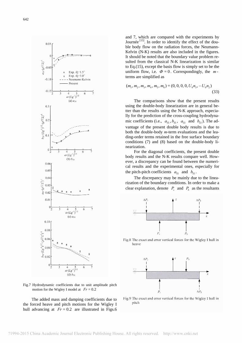
Fig.7 Hydrodynamic coefficients due to unit amplitude pitch

motion for the Wigley I model at = 0.2Fr

The added mass and damping coefficients due to

the forced heave and pitch motions for the Wigley I hull advancing at = 0.2Fr are illustrated in Figs.6

and 7, which are compared with the experiments by Journée [15]. In order to identify the effect of the dou- ble body flow on the radiation forces, the Neumann- Kelvin (N-K) results are also included in the figures. It should be noted that the boundary value problem re- sulted from the classical N-K linearization is similar to Eq.(15), except the basis flow is simply set to be the uniform flow, i.e. = 0 . Correspondingly, the -m terms are simplified as

1 2 3 4 5 6 0 3 0 2( , , , , , ) = (0, 0, 0, 0, , )m m m m m m U n U n

(33)

The comparisons show that the present results using the double-body linearization are in general be- tter than the results using the N-K approach, especia- lly for the prediction of the cross-coupling hydrodyna- mic coefficients (i.e., 35a , 35b , 53a and 53b ). The ad-

vantage of the present double body results is due to both the double-body m-term evaluations and the lea- ding-order terms retained in the free surface boundary conditions (7) and (8) based on the double-body li- nearization.

For the diagonal coefficients, the present double body results and the N-K results compare well. How- ever, a discrepancy can be found between the numeri- cal results and the experimental ones, especially for the pitch-pitch coefficients 55a and 55b .

The discrepancy may be mainly due to the linea- rization of the boundary conditions. In order to make a clear explanation, denote sP and bP as the resultants

Fig.8 The exact and error vertical forces for the Wigley I hull in

heave Fig.9 The exact and error vertical forces for the Wigley I hull in

pitch

643

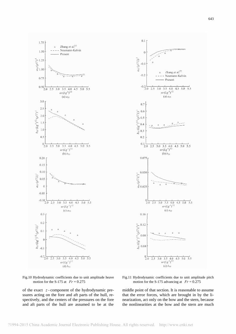
Fig.10 Hydrodynamic coefficients due to unit amplitude heave

motion for the S-175 at = 0.275Fr

of the exact -z component of the hydrodynamic pre- ssures acting on the fore and aft parts of the hull, re- spectively, and the centers of the pressures on the fore and aft parts of the hull are assumed to be at the

Fig.11 Hydrodynamic coefficients due to unit amplitude pitch

motion for the S-175 advancing at = 0.275Fr

middle point of that section. It is reasonable to assume that the error forces, which are brought in by the li- nearization, act only on the bow and the stern, because the nonlinearities at the bow and the stern are much

644

stronger than at the middle part of the hull. In the fo- llowing analysis, these error forces are denoted by

sP and bP , for the stern and the bow, respecti-

vely. When the Wigley I hull is forced to heave (see

Fig.8), sP and bP . are of the same sign, therefore

the summation of error forces will be added into the heave-heave force, which will result in an error in 33a

and 33b . However, the error moments caused by sP

and bP will cancel each other, so the prediction of

the pitch-heave coefficients 53a and 53b is satisfa-

ctory. When the Wigley I hull is forced to pitch (see Fig.9), sP and bP are of the similar magnitude but

of opposite sign. In this case, the prediction of the heave-pitch coefficients 35a and 35b is good because

sP and bP cancel each other. But an error moment

will be introduced. Although the magnitudes of sP

and bP are small, the long arm of the force (almost

two times of the arm between sP and bP ) will ampli-

fy the error greatly. Therefore, the discrepancies in

55a and 55b between the numerical results and the ex-

perimental ones are more remarkable than those in 33a

and 33b . For a more accurate prediction of these coe-

fficients, a nonlinear computation might be necessary. The hydrodynamic coefficients due to the forced

heave and pitch motions for the S-175 container ship are shown in Figs.10 and 11. Since experimental data are not available, the numerical results by Zhang et al.[7] are used to validate the present numerical calcu- lation. Their solution is based on the linearized free surface conditions and the exact body boundary condi- tion.

In general, good agreement can be found be- tween the numerical results from the present double body method and the method of Zhang et al.[7]. Dis- crepancies mainly occur in the prediction of the dam- ping coefficients 53b and 33b . The reason for these

discrepancies can be probably attributed to the differe- nt treatment of the body boundary condition. 3.3 Diffraction problem

Numerical simulations of the diffraction are ca- rried out for the Wigley I hull advancing in a regular head wave, with the forward speeds =Fr 0.2 and 0.3. The nondimensional incident wave length / L va- ries from 0.75 to 2.0. Similar to the radiation force, the wave exciting force is also transformed into the frequency domain and compared with the N-K solu- tions and with the experimental data[15].

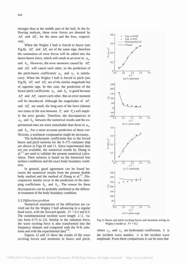
Figures 12 and 13 show the results of the wave exciting forces and moments in heave and pitch,

Fig.12 Heave and pitch exciting forces and moments acting on

Wigley I model at = 0.2Fr

where 33c and 55c are hydrostatic coefficients, k is

the incident wave number, A is the incident wave amplitude. From these comparisons it can be seen that

645

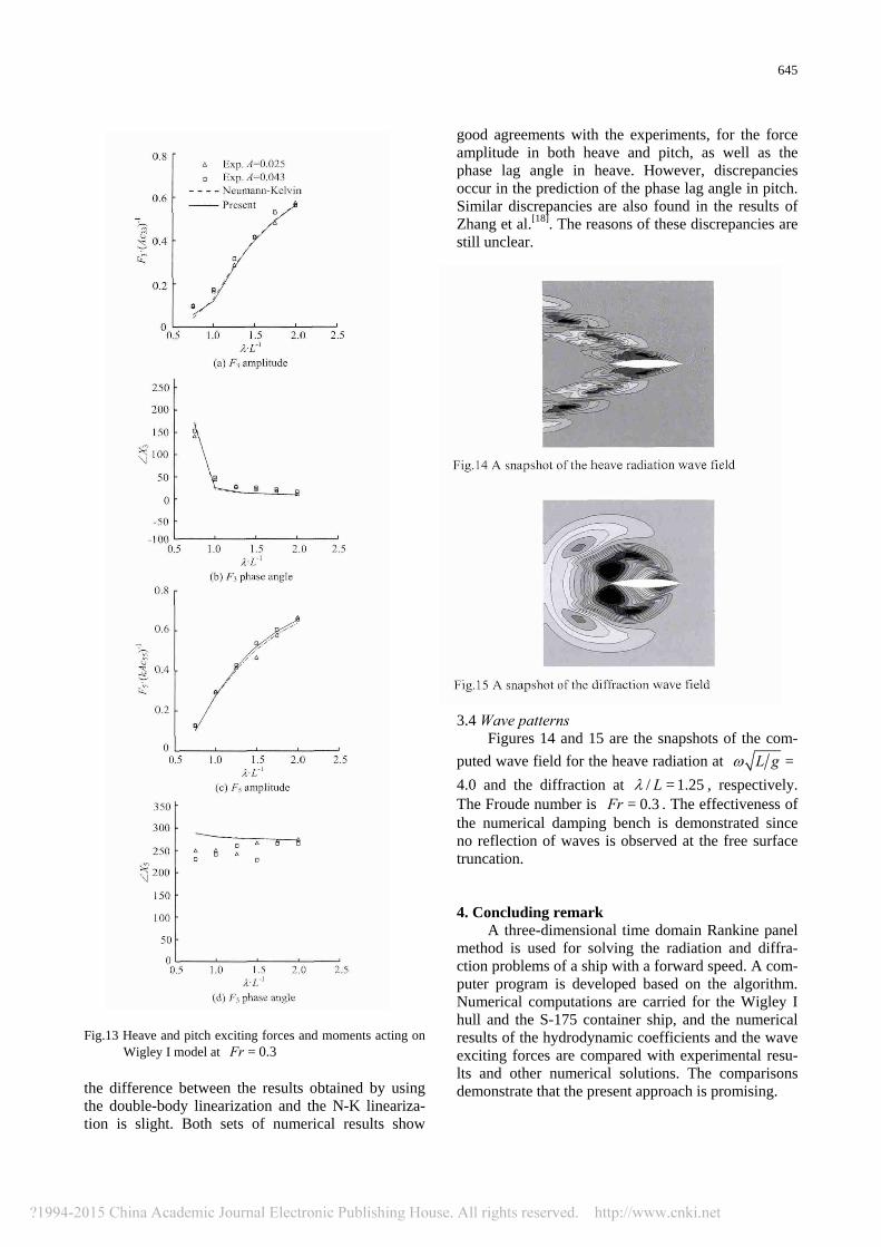
Fig.13 Heave and pitch exciting forces and moments acting on

Wigley I model at = 0.3Fr

the difference between the results obtained by using the double-body linearization and the N-K lineariza- tion is slight. Both sets of numerical results show

good agreements with the experiments, for the force amplitude in both heave and pitch, as well as the phase lag angle in heave. However, discrepancies occur in the prediction of the phase lag angle in pitch. Similar discrepancies are also found in the results of Zhang et al.[18]. The reasons of these discrepancies are still unclear. Fig.14 A snapshot of the heave radiation wave field Fig.15 A snapshot of the diffraction wave field 3.4 Wave patterns

Figures 14 and 15 are the snapshots of the com-

puted wave field for the heave radiation at =L g

4.0 and the diffraction at / = 1.25L , respectively. The Froude number is = 0.3Fr . The effectiveness of the numerical damping bench is demonstrated since no reflection of waves is observed at the free surface truncation. 4. Concluding remark

A three-dimensional time domain Rankine panel method is used for solving the radiation and diffra- ction problems of a ship with a forward speed. A com- puter program is developed based on the algorithm. Numerical computations are carried for the Wigley I hull and the S-175 container ship, and the numerical results of the hydrodynamic coefficients and the wave exciting forces are compared with experimental resu- lts and other numerical solutions. The comparisons demonstrate that the present approach is promising.

646

Acknowledgement ʼThis work was supported by the Lloyd s

Register Foundation (LRF). LRF helps to protect life and pro- perty by supporting engineering-related education, public engagement and the application of research. References [1] DATTA R., SEN D. A b-spline solver for the forward-

speed diffraction problem of a floating body in the time domain[J]. Applied Ocean Research, 2006, 28(2): 147-160.

[2] DUAN W., DAI Y. Integration of the time-domain Green function[C]. Twenty-second International Wo- rkshop on Water Waves and Floating Bodies. Plitvice, Croatia, 2007.

[3] ZHU Ren-chuan, ZHU Hai-rong and SHEN Liang et al. Numerical treatments and applications of the 3D tran- sient green function[J]. China Ocean Engineering, 2007, 21(4): 92-101.

[4] NAKOS D. E., KRING D. C. and SCLAVOUNOS P. D. Rankine panel methods for transient free-surface flows[C]. Sixth International Conference on Numeri- cal Ship Hydrodynamic. Iowa City, USA, 1993.

[5] HUANG Y. Nonlinear ship motions by a Rankine panel method[D]. Doctoral Thesis, Cambridge, MA, USA: Massachusetts Institute of Technology, 1997.

[6] KIM Y., KIM K. and KIM J. et al. Time domain analy- sis of nonlinear motion responses and structural loads on ships and offshore structures: Development of WISH programs[J]. International Journal of Naval Archite- cture and Ocean Engineering, 2011, 3(1): 37-52.

[7] ZHANG X., BANDYK P. and BECK R. F. Time-do- main simulations of radiation and diffraction forces[J]. Journal of Ship Research, 2010, 54(2): 79-94.

[8] YASUKAWA H. Time domain analysis of ship motions

inwaves using BEM (2nd Report: Motions in regular head waves)[J]. Transactions of the West-Japan So- ciety of Naval Architects, 2001, 101: 27-36.

[9] HE G., KASHIWAGI M. A time-domain higher-order boundary element method for 3D forward-speed radia- tion and diffraction problems[J]. Journal of Marine Science and Technology, 2014, 19(2): 228-244.

[10] CHEN Jing-pu, ZHU De-xiang. Numerical simulations of wave-induced ship motions in time domain by a Rankine panel method[J]. Journal of Hydrodynamics, 2010, 22(3): 373-380.

[11] CHEN Jing-pu, ZHU De-xiang. Numerical simulations of wave-induced ship motions in regular oblique waves by a time domain panel method[J]. Journal of Hydro- dynamics, 2010, 22(5): 419-426.

[12] CHEN Jing-pu, ZHU De-xiang. Numerical simulations of nonlinear ship motions in waves by a Rankine panel method[J]. Chinese Journal of Hydrodynamics, 2010, 25(6): 830-836(in Chinese).

[13] NEWMAN J. N. The theory of ship motions[J]. Adva- nces in Applied Mechanics, 1978, 18: 221-283.

[14] SALOMON D. Curves and surfaces for computer graphics[M]. New York, USA: Springer, 2005.

[15] JOURNÉE J. M. J. Experiments and calculations on four Wigley hull forms[R]. Technical Report 909. Delft, The Netherlands: Delft University of Technology, 1992.

[16] FONSECA N., GUEDES SOARES C. Comparison of numerical and experimental results of nonlinear wave- induced vertical ship motions and loads[J]. Journal of Marine Science and Technology, 2002, 6(4): 193-204.

[17] WU G. A numerical scheme for calculating the mj terms in wave-current-body interaction problem[J]. Applied Ocean Research,1991, 13(6): 317-319.

[18] ZHANG X., BANDYK P. and BECK R. F. Seakeeping computations using double-body basis flows[J]. App- lied Ocean Research, 2010, 32(4): 471-482.