Embed Size (px)
Citation preview

1
Time‐Space Kriging to Address the Problems of Misalignment, Mismatch and Missing Values in Spatiotemporal Datasets
Dong Liang1 & Naresh Kumar1
Department of Geography University of Iowa Iowa City, IA 52242
Email: naresh‐[email protected]
1 Department of Geography, University of Iowa, Iowa City, IA – 52242 Contact Email: naresh‐[email protected] NOTE: please do not quote or cite this work without our permission.

2
Abstract: The data from sensors aboard sun‐synchronous satellites are being used extensively to develop indirect estimates of socio‐physical environment in a cost‐effective manner. Irregular spatial distribution (due to offset in the satellite path) and data gaps across geographic space and time are two major challenges of satellite data, for example cloud cover during the satellite crossing time constrains retrieval of data. In this research, we address these two problems with the aid of an efficient time‐space Kriging method. We utilize the satellite based estimate of particulate matter ≤ 2.5µm in aerodynamic diameter (PM2.5) to develop a systematic grid of daily PM2.5 at 2.5km spatial resolution from 2000 to 2009 for Cleveland Metropolitan Statistical Area (MSA).
Even though there are gaps in the satellite based PM2.5 data, the number of data points in a given time and space interval is very large. Consequently, standard Kriging methods become computationally prohibitive for such datasets due to the O(n3) matrix decomposition. We conducted this study to derive an approximate Kriging method called Markov Regional Kriging for large datasets. In this study, point source data were regionalized into time‐space cubes and a hierarchical Bayesian smoothing model with Gaussian Markov Random Fields (GMRF) priors was proposed to approximate the time and space covariance function. GMRF structure matrices and Kronecker products were utilized to develop an efficient Markov chain Monte Carlo sampler based on the Conjugate Gradient algorithm. This method was validated using the PM2.5 dataset for Cleveland MSA. The 75% (~22,937) of data points predicted were comparable with that predicted using the local Kriging. But for 25% of data points local Kriging outperformed GMRF. GMRF can approximate non‐separable and non‐stationary time space covariance function for the air pollution (and potentially for other environmental) dataset. Our analysis suggests that among many methods of time‐space Kriging, GMRF smoothing offers a computationally efficient solution to address the problem of spatiotemporal misalignment in large dataset.
3
Introduction: Blurring disciplinary boundaries and converging time and space domains are important developments for interdisciplinary multilevel research. While such research can help us understand complex patterns of socio‐physical phenomena and processes that operate at multiple levels and shape these patterns, it require data from multiple sources and face three important challenges. First, the location and time stamps of these data (meaning when and where these data are monitored/recorded) are very different. This is referred to as the problem of spatiotemporal misalignment, because location and time of these data do not align. Second, spatiotemporal scales/resolutions of these data are subtly different. This means, spatiotemporal scales/resolutions at which these data are aggregated and reported are very different. Third, often these data suffer from missing values across geographic space and time. Analysis of these data requires that these data are aligned (by location and time), arranged on the same spatiotemporal scales and missing values are filled. For example, we need to estimate exposure (using air pollution data) at the spatiotemporal scale of mortality data to evaluate the association between ambient air pollution and mortality. Finest spatial resolution of mortality data is point location (i.e. street address of decedents) and the temporal scale is date of mortality. Daily exposure estimates are required several days prior to the date of death at the location of residence for each case or these data should be aggregated to coarser spatiotemporal scale. If adequate data points, spread across geographic space and time, are available, different methods of interpolation or imputation can be employed to estimate value at a given location and time. Among many methods, time‐space Kriging is a lucrative option because Kriging minimize the mean squared prediction errors among linear unbiased predictors.
Although time‐space Kriging is relatively a newer development, spatial Kriging has been in practice for a while. It relies on the assumption of spatial stationarity, which assumes that the covariance of a given variable is stationary (constant) across geographic space. It requires an understanding of how a quantity varies with respect to that observed at the neighboring sites (located at different distance intervals) to develop an empirical model to estimate semivariance with respect to geographic distance. Kriging has been used extensively in geostatisitcs literature to develop continuous surface of environmental variables (Cressie 1993, 2008). Although the extension of spatial Kriging to time‐space domain is straight forwards, implementation of time‐space Kriging can be challenging for several reasons. First, computationally, it can be difficult to implement, especially for large dataset. Because Kriging involves inversion of a dense square matrix of order n, where n denotes the number of observed data points. Second, stationarity assumption may not hold across both geographic space and time. Unlike spatial Kriging, time‐space Kriging involves estimation of covariance by geographic space, time and inseparable time‐space. Spatial covariance represents the variance present due to inherent geographic differences in the phenomena in question. Temporal covariance represents the variance occurring due to time. And time‐space covariance is associated with the variance that results from the interaction of spatial and temporal variance. An accurate prediction (at a given location and time) requires the proper specification of covariance function by time, space and space and time. This paper offers computationally efficient solutions to implement time‐space Kriging in large dataset, and evaluates prediction performance of Markov Regional Kriging (MRK) with the local time‐space Kriging. The remainder of this paper is organized into four sections. First section presents a summary of the recent developments in time‐space Kriging, followed by theoretical descriptions of time‐space MRK and local time‐space Kriging. The last two sections include result and a discussion of our results with the relevant literature.
Literature Review: Kriging is most widely used geostatistical method for spatial prediction (Lam 1983). Suppose that the observed data are the realization of an intrinsic stationary process (Cressie 1993) and the covariance function is known, values can be predicted at any given location. Let Z(si) denote n

4
observed data points and s0 denote the spatial location where prediction is needed. Kriging minimizes the mean squared errors among all unbiased predictors: min ∑ ; subject to
∑ 1 where λi denotes weight. In practice, the variogram 2 must
be estimated from the observed data based on the stationarity assumption. Given an estimated
variogram , the weights can be obtained by solving the Kriging equation. Building on the stationary assumption spatial Kriging can be extended to time‐space domain; Kriging by time and space involves prediction at a given location and time based on observed data points , . Although a number of studies demonstrate the application of time‐space Kriging (De Cesare, Myers and Posa 2001, 2002, De Iaco, Myers and Posa 2002, 2003, Spadavecchia and Williams 2009), several concerns remain to implement time‐space Kriging, including non‐separability of covariance by time and space, non‐stationarity across time and space and computation issues, especially for large dataset. The literature review here provides a summary of the basic time‐space Kriging models and then focuses on computational issues.
Time‐space Kriging requires specification and estimation of a spatiotemporal covariance function, which needs to be positive definite. In case, the function C(h,u) depends only on the spatial lag h and time lag u, it is called stationary. Stationary covariance functions in spatial domain are described in several textbooks (Cressie 1993, Banerjee, Carlin and Gelfand 2004). Extension of Kriging to time‐space domain requires decomposition of covariance by time and space, because the covariance by spatial lags may not correspond with the temporal lags, and some component of covariance is non‐separable by time and space. Several studies are available that address the issues of separable and non‐separable spatiotemporal covariance (Cressie and Huang 1999, De Iaco, Myers and Posa 2001, Kolovos, Christakos, Hristopulos and Serre 2004). Separable specification decomposes the cross‐covariance C(h,u) multiplicatively as C(h,u)=Cs(h)Ct(u), where Cs and Ct are spatial and temporal only covariance functions. Separable specification imposes restrictions on ranges of spatial correlation across time as well as ranges of temporal correlation over space. Non‐separable time‐space covariance function without the range restrictions have been proposed using product sum models (De Iaco, et al. 2001). A rich class of non‐separable covariance function can be generated by constructing spectral densities (Cressie, et al. 1999), partial differential equations representing physical laws and general stochastic theory (Kolovos, et al. 2004).
Time‐space Kriging is computationally intensive as it involves inversion of a dense square matrix of order n; where n denotes the number of observed data points. This calculation is O(n3) in computational time and O(n2) in storage. For large datasets, such as high resolution satellite data with the repetitive coverage, the computation becomes infeasible. This problem is termed as the big n problem (Banerjee, et al. 2004). In the remainder of this section, we review recent developments on the implementation of time‐space Kriging for large dataset.
There are two potential solutions to address the big n problem: local Kriging by reducing the number of data points and model based approximations to Kriging. Reducing the observed data points within the chosen distance and time lags is useful when prediction is required for a small number of locations. Specification of spatiotemporal lags requires substantive knowledge of the underlying process, because very small lags can results in very few data points that may not be enough for the estimation of covariance. Large spatiotemporal lags may introduce non‐stationarity in the data and lead to difficulties in modeling the time‐space covariance. In addition, local neighborhood approach is sensitive to missing data and outliers may generate gaps in the predicted values across time and space. A formal localized approach approximates the covariance function by tapering the function beyond a certain distance, assuming independence for data points beyond the given thresholds. Sparse matrix algorithms then

5
facilitate likelihood evaluation and Kriging (Furrer, Genton and Nychka 2006, Kaufman, Schervish and Nychka 2008).
Model based approximations to time space covariance have been proposed to address Kriging of large datasets. Bochner's theorem allows for efficient approximation of time space covariance by constructing spectral densities (Yao and Journel 1998). The Fast Fourier Transform also facilitates efficient evaluation of the covariance function and the corresponding Kriging for large datasets (Hoef, Cressie and Barry 2004). But the spectral approximation is most suitable for stationary covariance functions and the accuracy of approximation by truncation of higher frequency terms remains unclear. Some researchers also suggest multi‐resolution basis functions to estimate non‐stationary dependence in the data, which can facilitate efficient Kriging for large dataset (Nychka, Wikle and Royle 2002, Cressie, et al. 2008). The fixed rank Kriging approach approximates spatial covariance through a linear combination of fixed number of basis functions. The basis functions are multi‐resolution and generated by wavelet methods. The resulting Kriging calculation is exact and involves inversion of matrixes of fixed rank independent of the sample size. The fixed rank Kriging is generalized to fixed rank filtering in time‐space domain. Vector auto‐regression process and Kalman filter can also be used to incorporate temporal dependence to improve fixed rank Kriging when large gaps are present across space and time (Cressie, Shi and Kang 2010, Kang, Cressie and Shi 2010). These methods require an empirical estimation of variogram from the data and associated covariates.
An alternative to dimension reduction and approximation of Kriging is the predictive process for large spatial data in a Bayesian formulation (Banerjee, Gelfand, Finley and Sang 2008, Finley, Sang, Banerjee and Gelfand 2009, Banerjee, Finley, Waldmann and Ericsson 2010). This approach involves selection of small number of knots for filling the study space and develops a predictive process using the Kriging value of the original process on the knots. The resulting predictive process can capture non‐stationary covariance. The computation involves inversion of matrixes of the fixed rank. The projection of data onto a grid is not needed as in other knot based approaches. But the knots need to be chosen densely relative to the range of local spatial correlation, and nugget effects needs to be introduced to accurately estimate the variance components (Finley, et al. 2009).
Gaussian Markov random fields (GMRF) (Rue and Held 2006, Hartman and Hossjer 2008) approximation has recently been developed to approximate Kriging of large spatial data. Utilizing the GMRF approximation of the underlying Gaussian field, sparse matrix algorithms can be employed for solving Kriging equation for large datasets. This approach requires aligning the data onto a regular grid thus is ideal for lattice data. The choice of the grid and neighborhood needs to be fine tuned so that projection can be performed without much error. In addition, GRMF approximation requires knowledge about the covariance function of the target Gaussian process.
In this paper, we propose an alternative GMRF approximation to time‐space covariance functions and Kriging method termed Markov Regional Kriging (MRK) for large spatiotemporal datasets. Based on time‐space disease mapping models for areal data (Schmid and Held 2004), we estimate a nonstationary and nonseparable time‐space covariance function from the point data. The computational gain of GMRF approximation facilitates Bayesian inference based on MCMC methods. To demonstrate the application of this method, we utilized satellite based air pollution data for Cleveland MSA. These data exhibit non‐stationary time and space dependence, and extensive gaps across time and space. The next section provides a theoretical frame of the proposed along with local Kriging.
6
Theoretical Framework
Markov Regional Kriging model: The term regional in the context of this paper refers to as a subset of spatiotemporal domain under study, within which similarity in given variable is observed. If the entire spatiotemporal (organized across geographic space and time) is one big cube, a set of data points within this cube that possess similarities (in a variable under investigator) can refer to as region. Let , denote a Gaussian process defined over 1,2, … , where ⊂ . We assume that the process consists a structured but un‐observed process , and an un‐structured process , such that
, , ,
where Var , , 0 and , denotes known weight. Our model draws inference
of the un‐observed process given the observations. The hidden process is assumed to have a linear mean structure
, , ,
where , represents a vector of known covariates. The coefficients , … , are
unknown. The process , has zero means and a general time‐space covariance function , , , that captures the stochastic dependence of the process.
A class of non‐stationary covariance function can be specified via Gaussian Markov Random Fields (GMRF) approximation (Rue, et al. 2006): select a set of knots over the study area . This set of knots defines a tessellation of into non‐overlapping regions. Likewise select another set of knots over time points; where . Let and denote the region and time interval identifier of time‐space location , . The time‐space tessellation partitions the domain into small spatiotemporal domain, we call them cubes. Let denote the total number of such cubes. We decompose the time‐space component , as follows
, ,
where the regional factor does not change frequently and the temporal factor remains constant over space. The factor models local stochastic dependence and variation across time and space.
A model of stochastic dependence of the regional effects induces a covariance model of the original process. Utilizing the regular tessellation, the notion of spatiotemporal neighborhood is well defined. We can utilize GMRF (Besag 1974) to model these effects. Let denote a generic random effects, a GMRF model takes the form
∝ rg
exp2
where denotes a known structure matrix induced by a choice of neighborhood structure, rg denotes the rank of a matrix and denotes a unknown scale parameter of the field. Let and denote the eigenvectors of that corresponds to column and null space of and Λ denote the
rg diagonal matrix of positive eigen‐values of . Following Hodges, Carlin and Fan (2003) we can reparameterize as
| | 1
7
where and . The priors on and are apriori independent with flat prior on
and independent Gaussian prior on ∼ 0, Λ ; where ≡ .
Organize the regional effects onto an 1 vector , the temporal effects into a 1 vector and the time‐space effects into 1 vector , … , ordered region within time. We specify GMRF priors on , . Specifically, we adopt the conditional auto‐regression prior (Besag, York and Mollie 1991) on the regional effects and a random walk prior (Clayton 1996) on the temporal effects. The time‐space effects are constructed by Kronecker product where ⊗ (Clayton 1996). Following
the re‐parameterization, we have
∝ 1 and ∝ exp2
Λ for ∈ , , .
Let , and , , it follows that the covariance between two locations , and , under the model is
C , , , Λ Λ , Λ ,
where denotes the th row vector of a matrix . The induced covariance function is positive semi‐definite by construction, provided all variance parameters are strictly greater than zero. The eigen‐vectors of the GMRF structure matrixes serve as generator of the covariance. These vectors are typically multi‐resolution. Thus, they can capture multiple scales of time and space variation (Nychka, et al. 2002). Specifically, the covariance function does not depend on the spatiotemporal neighbors, and can capture non‐stationary behavior (Cressie, et al. 2008).
In practice, the process is observed at spatiotemporal locations , , 1, … , . Define the
vector of data ≡ , , , , … , , , arrange the 1 vector and in the manner
of . We have a general linear mixed model
where is an matrix of covariates. Let denote adjacency matrix with , 1
and zero otherwise. Define and in the similar manner to be the and adjacency
matrixes. The model then can be written as
.
Following the re‐parameterization (1), the above model may be written equivalently as
where denotes a matrix and ≡
, , , ; is a matrix, is an matrix and is an
matrix.
The above model is richly parameterized. Choices of fine resolution knots can easily lead to large number of cubes and many cubes as empty. The presence of empty cubes can lead to weak identification of the model from the data points. In the Bayesian framework, identification is equivalent to a proper posterior. Given the proper priors on , , , and , , ,
their posteriors are automatically proper and hence they are identified even without the data.
8
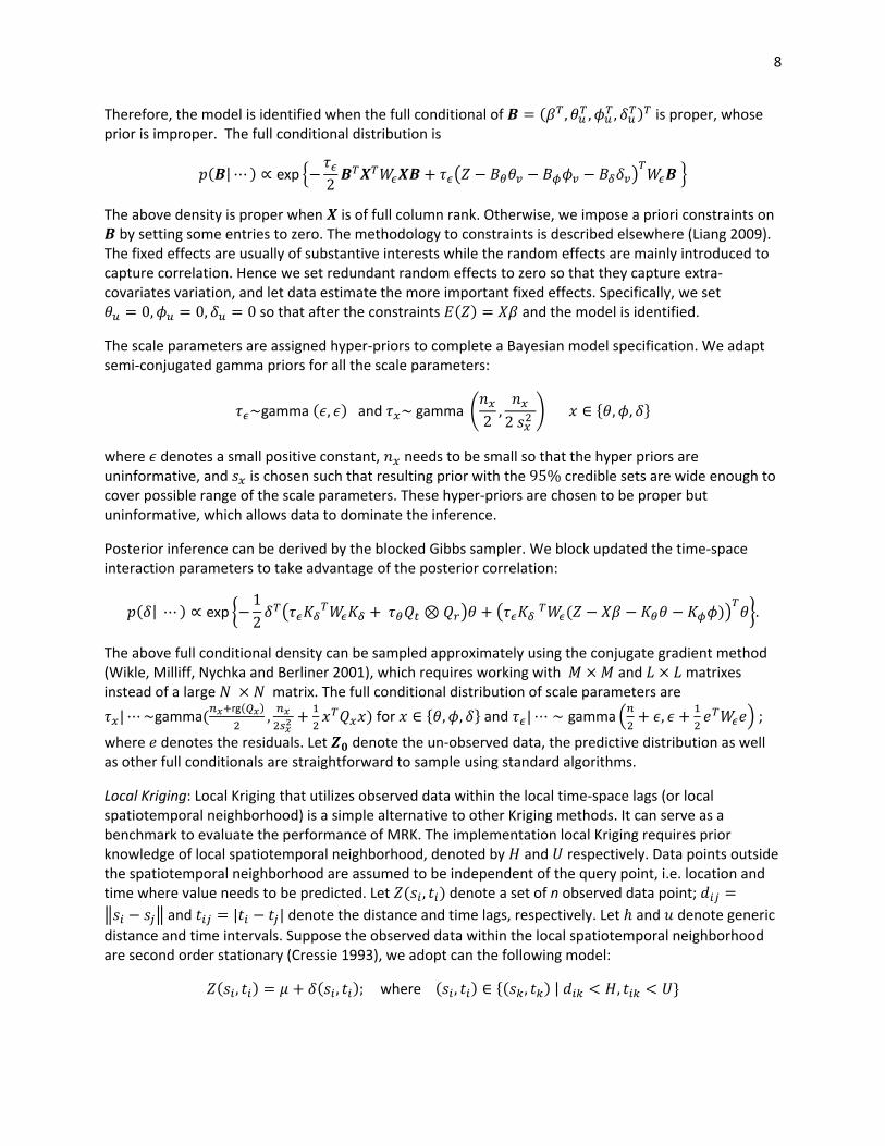
Therefore, the model is identified when the full conditional of , , , is proper, whose prior is improper. The full conditional distribution is
|⋯ ∝ exp2
The above density is proper when is of full column rank. Otherwise, we impose a priori constraints on by setting some entries to zero. The methodology to constraints is described elsewhere (Liang 2009).
The fixed effects are usually of substantive interests while the random effects are mainly introduced to capture correlation. Hence we set redundant random effects to zero so that they capture extra‐covariates variation, and let data estimate the more important fixed effects. Specifically, we set
0, 0, 0 so that after the constraints and the model is identified.
The scale parameters are assigned hyper‐priors to complete a Bayesian model specification. We adapt semi‐conjugated gamma priors for all the scale parameters:
~gamma , and ~ gamma 2,2
∈ , ,
where denotes a small positive constant, needs to be small so that the hyper priors are uninformative, and is chosen such that resulting prior with the 95% credible sets are wide enough to cover possible range of the scale parameters. These hyper‐priors are chosen to be proper but uninformative, which allows data to dominate the inference.
Posterior inference can be derived by the blocked Gibbs sampler. We block updated the time‐space interaction parameters to take advantage of the posterior correlation:
| ⋯ ∝ exp1
2 ⊗ .
The above full conditional density can be sampled approximately using the conjugate gradient method (Wikle, Milliff, Nychka and Berliner 2001), which requires working with and matrixes instead of a large matrix. The full conditional distribution of scale parameters are
|⋯~gammarg
,
for ∈ , , and |⋯ ∼ gamma , ;
where denotes the residuals. Let denote the un‐observed data, the predictive distribution as well as other full conditionals are straightforward to sample using standard algorithms.
Local Kriging: Local Kriging that utilizes observed data within the local time‐space lags (or local spatiotemporal neighborhood) is a simple alternative to other Kriging methods. It can serve as a benchmark to evaluate the performance of MRK. The implementation local Kriging requires prior knowledge of local spatiotemporal neighborhood, denoted by and respectively. Data points outside the spatiotemporal neighborhood are assumed to be independent of the query point, i.e. location and time where value needs to be predicted. Let , denote a set of n observed data point;
and | | denote the distance and time lags, respectively. Let and denote generic
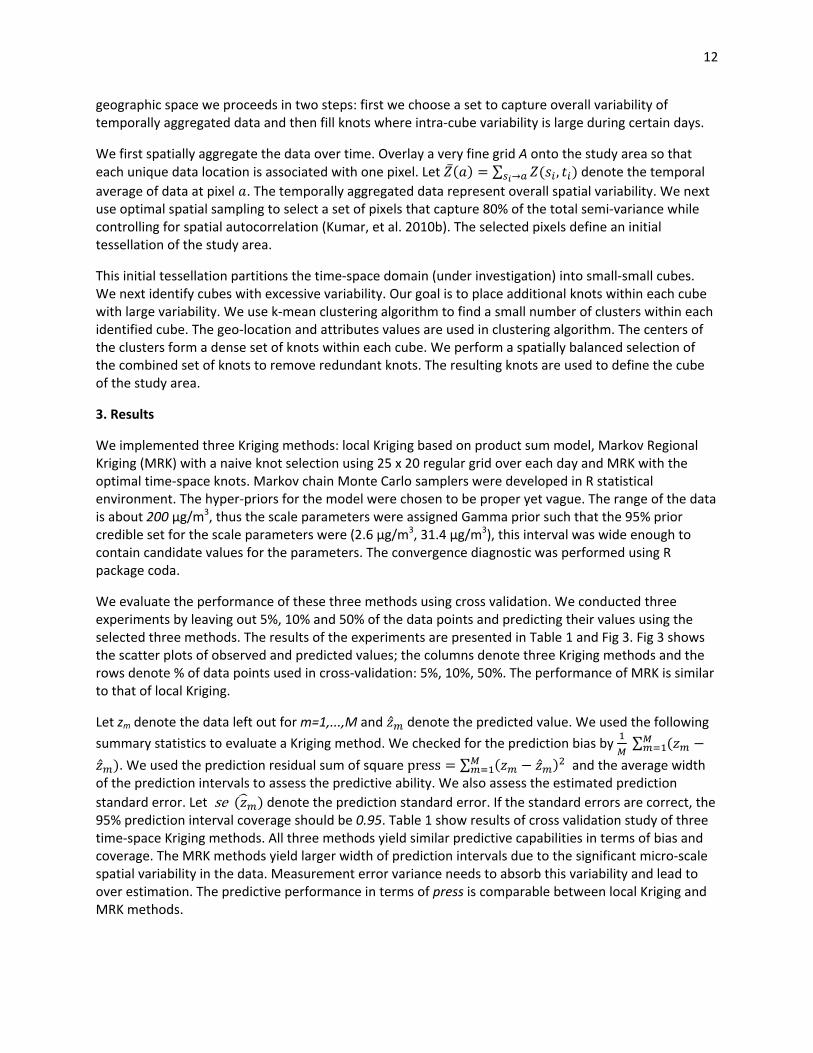
distance and time intervals. Suppose the observed data within the local spatiotemporal neighborhood are second order stationary (Cressie 1993), we adopt can the following model:
, , ; where , ∈ , | ,

9
where the time‐space covariance function , | COV , , , can be specified
using the product sum approach (De Iaco, et al. 2001), as
, | | | | |
where | and | are valid space and time only covariance functions and 0, 0 and 0 and denote the parameters for covariance functions.
Data and Implementation
2.1 Data – Airborne particulate ≤2.5µm in aerodynamic diameter (PM2.5), used in this study, were extracted using the data from MODerate Resolution Imaging Spectroradiometer (MODIS), aboard Terra and Aqua satellites. An empirical relationship between ground monitored PM2.5 and 2km AOD was established after controlling for meteorological conditions. Using this relationship PM2.5 was predicted for all data points when AOD values were available within the Cleveland MSA between 2000 and 2009. The total number of data points (for which daily PM2.5 was predicted) was > 2.3 million, and on an average 596 data points were available on a given day. The methodological details for the computation and validation of PM2.5 are provided elsewhere (Kumar, Chu, Foster, Peters and Willis 2010a).
2.2 Implementation – A 5km grid was overlaid on the study area (Fig 1a), and our objective was to estimate daily PM2.5 using the irregular PM2.5 data (Fig 1b) when and where the 2km AOD was available. We implemented Markov Regional Kriging (MRK) and local Kriging methods for developing a systematic grid of daily PM2.5 at 5km spatial resolution. Since the number of data points (in the observed dataset) was very large, we restricted our analysis between December 2001 and January 2003. While analyzing the PM2.5 data we learned about several data limitations and challenges that we face to implement Kriging by time and space on these data. Due to cloud cover and contamination, AOD retrievals were not possible. Therefore, there were systematic gaps in the PM2.5 data. During the span of 14 months, there were no observed data for about 41% of the days. The rate of spatiotemporal variability in PM2.5 was not the same, for example PM2.5 varied significantly by time than by geographic space. This can be attributed to the transport of PM2.5 due to meteorological conditions that can transport fine particulates at a greater pace and distance. Fig 2 shows time series plot of PM2.5 over a small area, along with the fitted temporal trend. The median of the lag one autocorrelations of fitted temporal trends over Cleveland MSA is 0.51 with 95 confidence interval (0.46, 0.66). The data show moderate temporal dependence. In the remainder of this section we describe implementation of local and MRK Kriging methods.
2.3 Implementation of local space‐time Kriging: To implement local time‐space Kriging we face with two important challenges: specification of local spatiotemporal neighborhood and non‐stationarity within the neighborhood. Narrow spatiotemporal lags can result in very few data points to accurately estimate time‐space covariance function (Kyriakidis and Journel 1999). Consequently, it will result in discontinuity in the prediction across time and space. For example, in the satellite based air pollution data, there are systematic gaps (due to cloud cover and/or data contamination) and sufficient data points may not be available if small time‐space lags are used to define the neighborhood. To ensure adequate sample size, we can divide the local neighborhood into non‐overlapping cubes. Let and denote the number of distinct cubes across space and time, we proceed with the following procedure
only when and for a given lower limits. For the demonstration purposes we set 3.
A wider specification of spatiotemporal lags can result in too many data points within the local neighborhood. Let , , , denote data points, the computation of Kriging involves inversion of
10
an matrix. If the number of data points is too large, inversion of a large square matrix becomes computationally prohibitive. Therefore, reducing the size of n is critically important for local Kriging. Among many options, we suggest subsampling data points within the local neighborhood to address the big n problem. This requires setting up an upper limit of the data points within the local neighborhoods. If the total number of data points exceed , we subsample data points. Specifically we divide the space and time domain into non‐overlapping regions and sample from each region. Let denote the sampling probability of region 1, … , , we assign ∝ the number of points in
each local spatiotemporal neighborhood. Even though this approach discards some data points, the loss of information is relatively small because of strong spatiotemporal autocorrelation within the neighborhood.
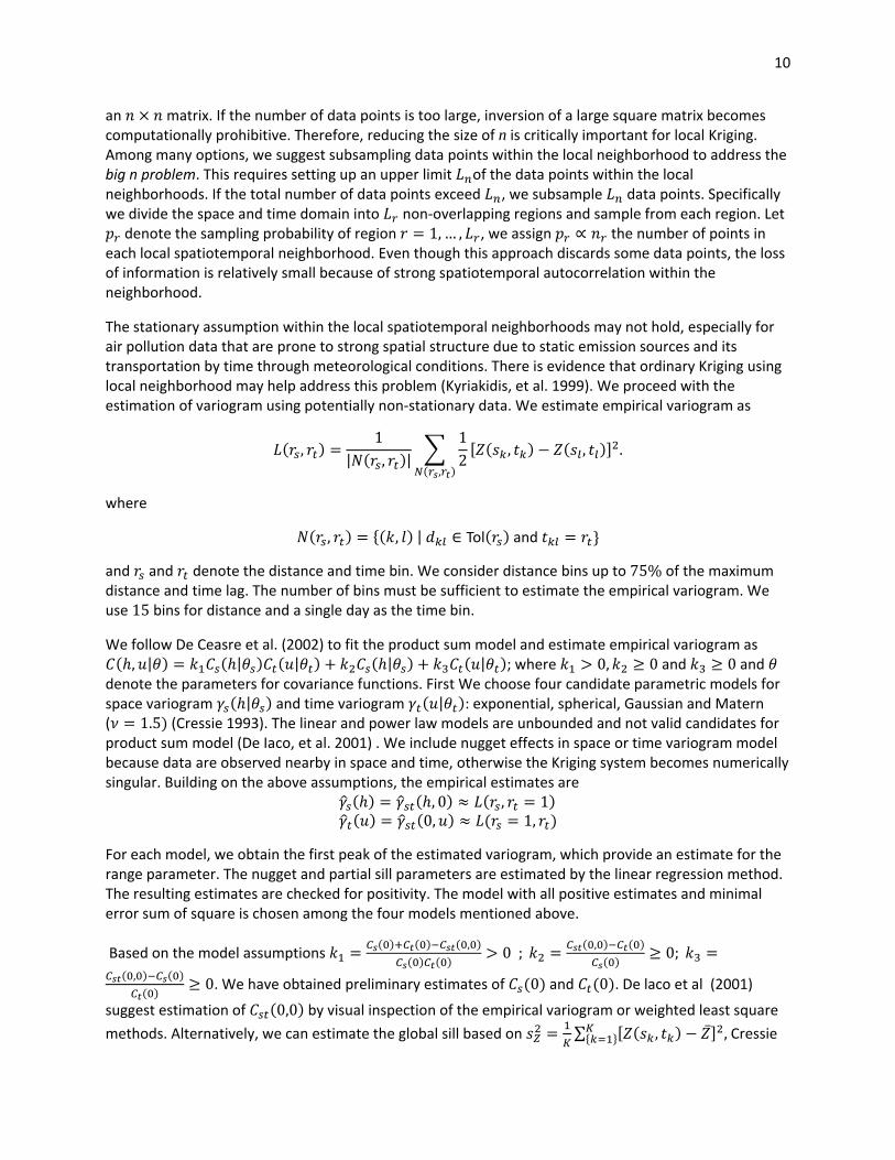
The stationary assumption within the local spatiotemporal neighborhoods may not hold, especially for air pollution data that are prone to strong spatial structure due to static emission sources and its transportation by time through meteorological conditions. There is evidence that ordinary Kriging using local neighborhood may help address this problem (Kyriakidis, et al. 1999). We proceed with the estimation of variogram using potentially non‐stationary data. We estimate empirical variogram as
,1
| , |
1
2, ,
,
.
where
, , | ∈ Tol and
and and denote the distance and time bin. We consider distance bins up to 75% of the maximum distance and time lag. The number of bins must be sufficient to estimate the empirical variogram. We use 15 bins for distance and a single day as the time bin.
We follow De Ceasre et al. (2002) to fit the product sum model and estimate empirical variogram as , | | | | | ; where 0, 0 and 0 and
denote the parameters for covariance functions. First We choose four candidate parametric models for space variogram | and time variogram | : exponential, spherical, Gaussian and Matern ( 1.5 (Cressie 1993). The linear and power law models are unbounded and not valid candidates for product sum model (De Iaco, et al. 2001) . We include nugget effects in space or time variogram model because data are observed nearby in space and time, otherwise the Kriging system becomes numerically singular. Building on the above assumptions, the empirical estimates are
, 0 , 1 0, 1,
For each model, we obtain the first peak of the estimated variogram, which provide an estimate for the range parameter. The nugget and partial sill parameters are estimated by the linear regression method. The resulting estimates are checked for positivity. The model with all positive estimates and minimal error sum of square is chosen among the four models mentioned above.
Based on the model assumptions ,
0 ; ,
0;
,0. We have obtained preliminary estimates of 0 and 0 . De laco et al (2001)
suggest estimation of 0,0 by visual inspection of the empirical variogram or weighted least square
methods. Alternatively, we can estimate the global sill based on ∑ , , Cressie
11
(1988) utilizes the following estimates for the sill to correct the bias in where K denotes number of neighbors:
0,0∑ ∑ | , |
∑ ∑ , | , |.
The preliminary estimates of 0 and 0 are adjusted so that 0 0 0,0
max 0 , 0 . As a result we obtain a fitted covariance model
, .
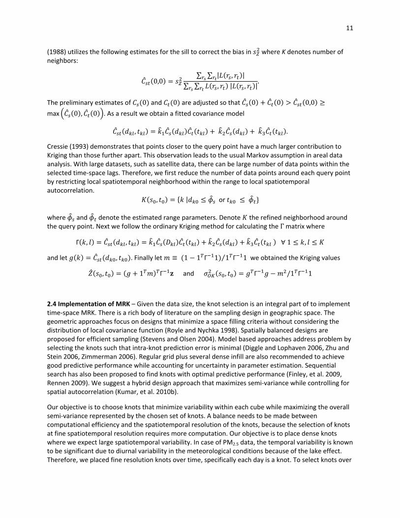
Cressie (1993) demonstrates that points closer to the query point have a much larger contribution to Kriging than those further apart. This observation leads to the usual Markov assumption in areal data analysis. With large datasets, such as satellite data, there can be large number of data points within the selected time‐space lags. Therefore, we first reduce the number of data points around each query point by restricting local spatiotemporal neighborhood within the range to local spatiotemporal autocorrelation.
, | or
where and denote the estimated range parameters. Denote the refined neighborhood around the query point. Next we follow the ordinary Kriging method for calculating the Γ matrix where
Γ , , ∀ 1 ,
and let , . Finally let ≡ 1 1 Γ 1 1 Γ 1⁄ we obtained the Kriging values
, 1 Γ and , Γ /1 Γ 1
2.4 Implementation of MRK – Given the data size, the knot selection is an integral part of to implement time‐space MRK. There is a rich body of literature on the sampling design in geographic space. The geometric approaches focus on designs that minimize a space filling criteria without considering the distribution of local covariance function (Royle and Nychka 1998). Spatially balanced designs are proposed for efficient sampling (Stevens and Olsen 2004). Model based approaches address problem by selecting the knots such that intra‐knot prediction error is minimal (Diggle and Lophaven 2006, Zhu and Stein 2006, Zimmerman 2006). Regular grid plus several dense infill are also recommended to achieve good predictive performance while accounting for uncertainty in parameter estimation. Sequential search has also been proposed to find knots with optimal predictive performance (Finley, et al. 2009, Rennen 2009). We suggest a hybrid design approach that maximizes semi‐variance while controlling for spatial autocorrelation (Kumar, et al. 2010b).
Our objective is to choose knots that minimize variability within each cube while maximizing the overall semi‐variance represented by the chosen set of knots. A balance needs to be made between computational efficiency and the spatiotemporal resolution of the knots, because the selection of knots at fine spatiotemporal resolution requires more computation. Our objective is to place dense knots where we expect large spatiotemporal variability. In case of PM2.5 data, the temporal variability is known to be significant due to diurnal variability in the meteorological conditions because of the lake effect. Therefore, we placed fine resolution knots over time, specifically each day is a knot. To select knots over
12
geographic space we proceeds in two steps: first we choose a set to capture overall variability of temporally aggregated data and then fill knots where intra‐cube variability is large during certain days.
We first spatially aggregate the data over time. Overlay a very fine grid A onto the study area so that each unique data location is associated with one pixel. Let ∑ ,→ denote the temporal
average of data at pixel . The temporally aggregated data represent overall spatial variability. We next use optimal spatial sampling to select a set of pixels that capture 80% of the total semi‐variance while controlling for spatial autocorrelation (Kumar, et al. 2010b). The selected pixels define an initial tessellation of the study area.
This initial tessellation partitions the time‐space domain (under investigation) into small‐small cubes. We next identify cubes with excessive variability. Our goal is to place additional knots within each cube with large variability. We use k‐mean clustering algorithm to find a small number of clusters within each identified cube. The geo‐location and attributes values are used in clustering algorithm. The centers of the clusters form a dense set of knots within each cube. We perform a spatially balanced selection of the combined set of knots to remove redundant knots. The resulting knots are used to define the cube of the study area.
3. Results
We implemented three Kriging methods: local Kriging based on product sum model, Markov Regional Kriging (MRK) with a naive knot selection using 25 x 20 regular grid over each day and MRK with the optimal time‐space knots. Markov chain Monte Carlo samplers were developed in R statistical environment. The hyper‐priors for the model were chosen to be proper yet vague. The range of the data is about 200 µg/m3, thus the scale parameters were assigned Gamma prior such that the 95% prior credible set for the scale parameters were (2.6 µg/m3, 31.4 µg/m3), this interval was wide enough to contain candidate values for the parameters. The convergence diagnostic was performed using R package coda.
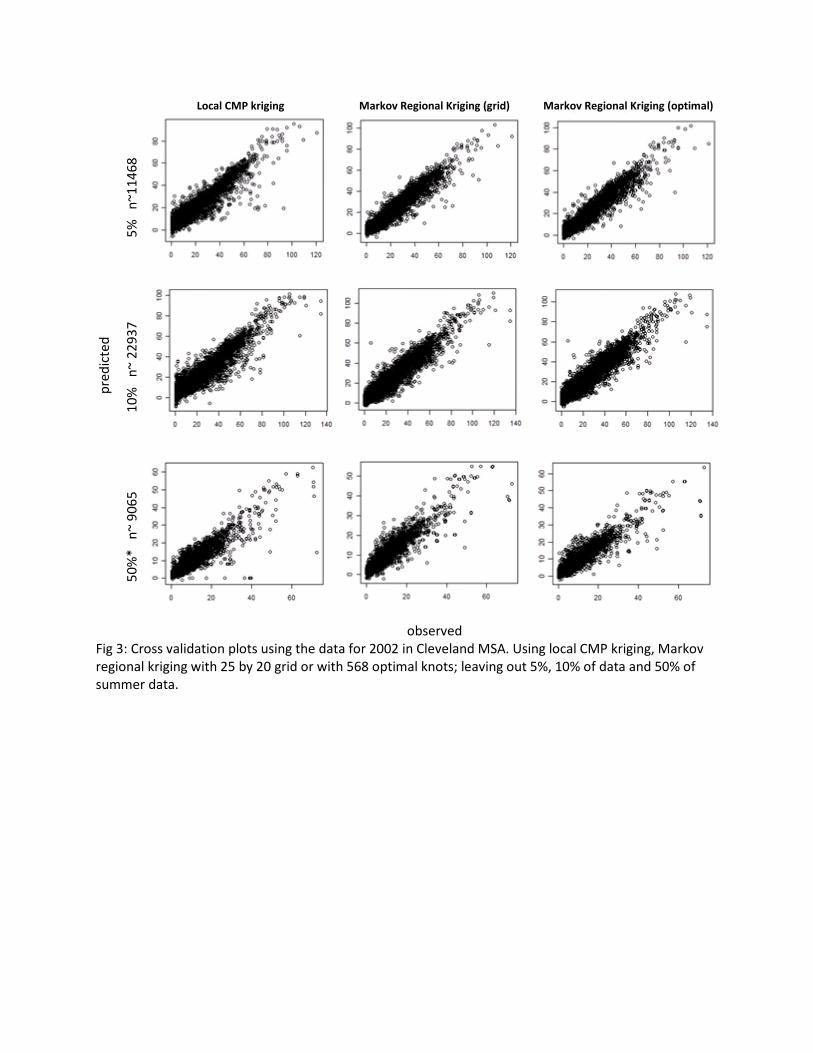
We evaluate the performance of these three methods using cross validation. We conducted three experiments by leaving out 5%, 10% and 50% of the data points and predicting their values using the selected three methods. The results of the experiments are presented in Table 1 and Fig 3. Fig 3 shows the scatter plots of observed and predicted values; the columns denote three Kriging methods and the rows denote % of data points used in cross‐validation: 5%, 10%, 50%. The performance of MRK is similar to that of local Kriging.
Let zm denote the data left out for m=1,...,M and denote the predicted value. We used the following
summary statistics to evaluate a Kriging method. We checked for the prediction bias by ∑
. We used the prediction residual sum of square press ∑ and the average width of the prediction intervals to assess the predictive ability. We also assess the estimated prediction
standard error. Let se denote the prediction standard error. If the standard errors are correct, the 95% prediction interval coverage should be 0.95. Table 1 show results of cross validation study of three time‐space Kriging methods. All three methods yield similar predictive capabilities in terms of bias and coverage. The MRK methods yield larger width of prediction intervals due to the significant micro‐scale spatial variability in the data. Measurement error variance needs to absorb this variability and lead to over estimation. The predictive performance in terms of press is comparable between local Kriging and MRK methods.

13
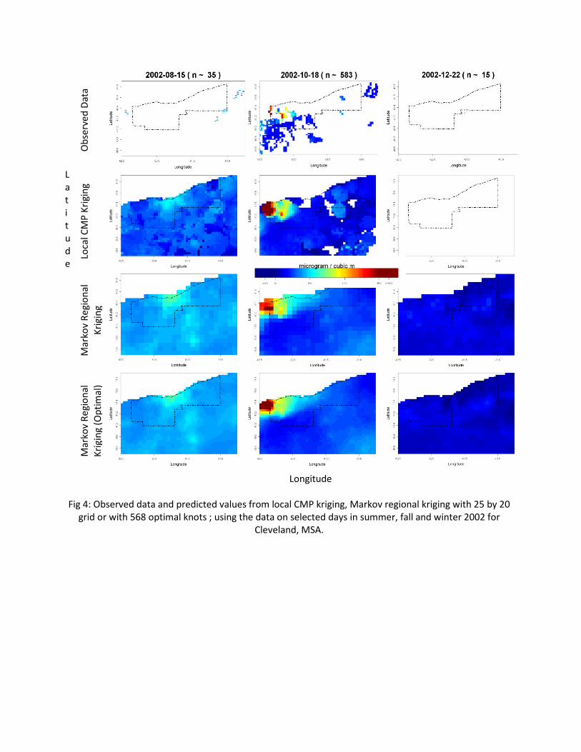
Fig 4 shows the observed data points and predicted surface on three different days: one each in summer, fall and winter of 2002. The columns represents dates, the first row shows the observed data and the remaining three rows show the predicting surface derived using the three selected methods: local Kriging, MRK with naïve knots and MRK with the optimal knots. Visual inspection of this figure suggests that the local Kriging captures the detailed spatial variation and outlier, present in the data (such as very high concentration of PM2.5 in the north western corner on October 28, 2002). However, MRK smoothes these outliers using the coarse spatiotemporal regional parameters. MRF provides a continuous surface and full spatial coverage while local Kriging can leads to gaps due to lack of data. For example, on December 12, 2002 local Kriging failed to provide any surface because of non‐availability of observed data within the time‐space lags used for defining local neighborhoods. With regard to computational performance, MRK is more efficient as compared to local Kriging, for example the running time for MRK on 10% of the data points was 4.99 hours including knot selection and simulation. However, the local Kriging took about 11.7 hours.
4. Discussion: Time‐space Kriging is an important method of prediction that can address multiple problems arising from the convergence of time and space domains – misalignment problem, missing values and mismatch in the spatiotemporal resolutions. This paper presents a theoretical framework of a computationally efficient MRK procedure for predicting a systematic grid of time‐space varying quantities. The performance of MRK was compared with the local time‐space Kriging. Both methods were implemented on air pollution data in Cleveland MSA. Significant diurnal variation and systematic large gaps in data across geographic space and time are two important characteristics of these data. Our analysis suggests that the MRK handled both these problems effectively and efficiently.
The MRK builds on Markov approximation of time‐space covariance and offers several advantages over the traditional Kriging methods. First, the proposed method exploits the sparseness and Kronecker structure of the precision matrixes of GMRF, so that Kriging can be performed on datasets which are computationally prohibitive (for classical Kriging methods). Second the MRK utilizes multi‐resolution eigen‐vectors to approximate non‐stationarity in data across time and space. Third, MRK ensures complete coverage prediction across time and space even when there are extensive gaps in the observed datasets.
Despite the above advantages, a number of limitations remain. First, it is difficult to model fine scale spatial variability using MRK. Our approach relies on the measurement error to capture the micro‐scale variation. As evident from the comparison of MRK estimate with that derived using local time‐space Kriging, MRK leads to positive bias in variance component estimation, and wide and conservative prediction intervals. Finley et al. (2009) introduce nugget effects to correct for micro‐scale variability. The future work will be geared towards implementing a similar approach to correct for this bias. Second, MRK is still computationally intensive when performing Kriging on large dataset that consists of large geographical area span across greater time interval without losing local spatiotemporal details. This issue can be addressed by integrated nested Laplace approximation of posterior marginal approximates (Rue, Martino and Chopin 2009). Cowles et al. (Cowles, Zimmerman, Christ and McGinnis 2002) suggest an alternate approach to combine large spatiotemporal datasets. They develop multiple levels of regions across space and model the spatial correlation separately and hierarchically within each level. Parallel computing is another solution to address the computation problem. Third, the choice of knots over time and space is still a challenging issue. We need to determine the time and spatial locations in the dataset that lead to best predictive performance. In this paper, first we identify optimal knots onto geographic space and then optimize knots over time for each geographic knots. Some researchers suggest varying knots over time and space, especially for MCMC sampling (Banerjee, et al. 2010). An alternate is to model the data as spatiotemporal mixtures of distribution centered around varying knots, which can be
14
assigned a prior distribution. This approach has been employed for mapping cancer risks (Knorr‐Held and Best 2001).
With the increasing availability of multi‐resolution spatiotemporal data from multiples sources, the use of time‐space Kriging is likely to increase in the future. We live in the era of geospatial information revolution in which convergence of spatiotemporal data and information from multiple sources and multiple sensors (with varying spatiotemporal scales) is inevitable. While this convergence is important for complexity research to develop an understanding of complex socio‐physical patterns and process that shape them, increasing data dimension and data size make it difficult to address the problem of spatiotemporal misalignment, mismatch in the spatiotemporal resolution/scales and gaps across space and time. As demonstrated in this paper, computationally efficient methods of time‐space Kriging hold the key to address these problems and we call for further research on computationally efficient time‐space Kriging models and algorithms that minimizes computation time and capture hierarchical (local, regional and global) spatio‐temporal structures in the data.
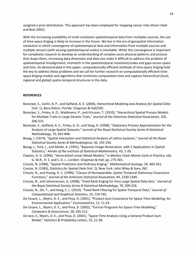
REFERENCES Banerjee, S., Carlin, B. P., and Gelfand, A. E. (2004), Hierarchical Modeling and Analysis for Spatial Data
(Vol. 1), Boca Raton, Florida: Chapman & Hall/CRC. Banerjee, S., Finley, A. O., Waldmann, P., and Ericsson, T. (2010), "Hierarchical Spatial Process Models
for Multiple Traits in Large Genetic Trials," Journal of the American Statistical Association, 105, 506‐521.
Banerjee, S., Gelfand, A. E., Finley, A. O., and Sang, H. (2008), "Stationary Process Approximation for the Analysis of Large Spatial Datasets," Journal of the Royal Statistical Society Series B‐Statistical Methodology, 70, 825‐848.
Besag, J. (1974), "Spatial Interaction and Statistical‐Analysis of Lattice Systems," Journal of the Royal Statistical Society Series B‐Methodological, 36, 192‐236.
Besag, J., York, J., and Mollie, A. (1991), "Bayesian Image‐Restoration, with 2 Applications in Spatial Statistics," Annals of the Institute of Statistical Mathematics, 43, 1‐20.
Clayton, D. G. (1996), "Generalized Linear Mixed Models," in Markov Chain Monte Carlo in Practice, eds. G. W.R., R. S. and S. D. J., London: Chapman & Hall, pp. 275‐301.
Cressie, N. (1988), "Spatial Prediction and Ordinary Kriging," Mathematical Geology, 20, 405‐421. Cressie, N. (1993), Statistics for Spatial Data (Vol. 2), New York: John Wiley & Sons, INC. Cressie, N., and Huang, H. C. (1999), "Classes of Nonseparable, Spatio‐Temporal Stationary Covariance
Functions," Journal of the American Statistical Association, 94, 1330‐1340. Cressie, N., and Johannesson, G. (2008), "Fixed Rank Kriging for Very Large Spatial Data Sets," Journal of
the Royal Statistical Society Series B‐Statistical Methodology, 70, 209‐226. Cressie, N., Shi, T., and Kang, E. L. (2010), "Fixed Rank Filtering for Spatio‐Temporal Data," Journal of
Computational and Graphical Statistics, 19, 724‐745. De Cesare, L., Myers, D. E., and Posa, D. (2001), "Product‐Sum Covariance for Space‐Time Modeling: An
Environmental Application," Environmetrics, 12, 11‐23. De Cesare, L., Myers, D. E., and Posa, D. (2002), "Fortran Programs for Space‐Time Modeling,"
Computers & Geosciences, 28, 205‐212. De Iaco, S., Myers, D. E., and Posa, D. (2001), "Space‐Time Analysis Using a General Product‐Sum
Model," Statistics & Probability Letters, 52, 21‐28.
15
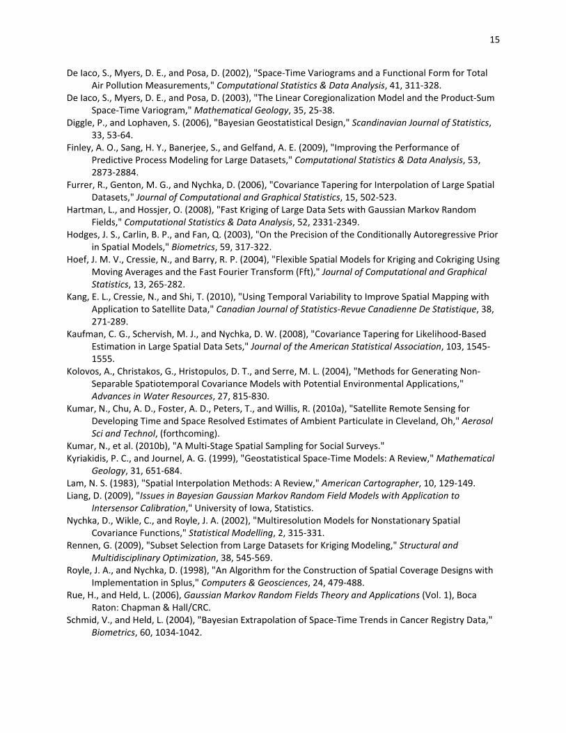
De Iaco, S., Myers, D. E., and Posa, D. (2002), "Space‐Time Variograms and a Functional Form for Total Air Pollution Measurements," Computational Statistics & Data Analysis, 41, 311‐328.
De Iaco, S., Myers, D. E., and Posa, D. (2003), "The Linear Coregionalization Model and the Product‐Sum Space‐Time Variogram," Mathematical Geology, 35, 25‐38.
Diggle, P., and Lophaven, S. (2006), "Bayesian Geostatistical Design," Scandinavian Journal of Statistics, 33, 53‐64.
Finley, A. O., Sang, H. Y., Banerjee, S., and Gelfand, A. E. (2009), "Improving the Performance of Predictive Process Modeling for Large Datasets," Computational Statistics & Data Analysis, 53, 2873‐2884.
Furrer, R., Genton, M. G., and Nychka, D. (2006), "Covariance Tapering for Interpolation of Large Spatial Datasets," Journal of Computational and Graphical Statistics, 15, 502‐523.
Hartman, L., and Hossjer, O. (2008), "Fast Kriging of Large Data Sets with Gaussian Markov Random Fields," Computational Statistics & Data Analysis, 52, 2331‐2349.
Hodges, J. S., Carlin, B. P., and Fan, Q. (2003), "On the Precision of the Conditionally Autoregressive Prior in Spatial Models," Biometrics, 59, 317‐322.
Hoef, J. M. V., Cressie, N., and Barry, R. P. (2004), "Flexible Spatial Models for Kriging and Cokriging Using Moving Averages and the Fast Fourier Transform (Fft)," Journal of Computational and Graphical Statistics, 13, 265‐282.
Kang, E. L., Cressie, N., and Shi, T. (2010), "Using Temporal Variability to Improve Spatial Mapping with Application to Satellite Data," Canadian Journal of Statistics‐Revue Canadienne De Statistique, 38, 271‐289.
Kaufman, C. G., Schervish, M. J., and Nychka, D. W. (2008), "Covariance Tapering for Likelihood‐Based Estimation in Large Spatial Data Sets," Journal of the American Statistical Association, 103, 1545‐1555.
Kolovos, A., Christakos, G., Hristopulos, D. T., and Serre, M. L. (2004), "Methods for Generating Non‐Separable Spatiotemporal Covariance Models with Potential Environmental Applications," Advances in Water Resources, 27, 815‐830.
Kumar, N., Chu, A. D., Foster, A. D., Peters, T., and Willis, R. (2010a), "Satellite Remote Sensing for Developing Time and Space Resolved Estimates of Ambient Particulate in Cleveland, Oh," Aerosol Sci and Technol, (forthcoming).
Kumar, N., et al. (2010b), "A Multi‐Stage Spatial Sampling for Social Surveys." Kyriakidis, P. C., and Journel, A. G. (1999), "Geostatistical Space‐Time Models: A Review," Mathematical
Geology, 31, 651‐684. Lam, N. S. (1983), "Spatial Interpolation Methods: A Review," American Cartographer, 10, 129‐149. Liang, D. (2009), "Issues in Bayesian Gaussian Markov Random Field Models with Application to
Intersensor Calibration," University of Iowa, Statistics. Nychka, D., Wikle, C., and Royle, J. A. (2002), "Multiresolution Models for Nonstationary Spatial
Covariance Functions," Statistical Modelling, 2, 315‐331. Rennen, G. (2009), "Subset Selection from Large Datasets for Kriging Modeling," Structural and
Multidisciplinary Optimization, 38, 545‐569. Royle, J. A., and Nychka, D. (1998), "An Algorithm for the Construction of Spatial Coverage Designs with
Implementation in Splus," Computers & Geosciences, 24, 479‐488. Rue, H., and Held, L. (2006), Gaussian Markov Random Fields Theory and Applications (Vol. 1), Boca
Raton: Chapman & Hall/CRC. Schmid, V., and Held, L. (2004), "Bayesian Extrapolation of Space‐Time Trends in Cancer Registry Data,"
Biometrics, 60, 1034‐1042.

16
Spadavecchia, L., and Williams, M. (2009), "Can Spatio‐Temporal Geostatistical Methods Improve High Resolution Regionalisation of Meteorological Variables?," Agricultural and Forest Meteorology, 149, 1105‐1117.
Stevens, D. L., and Olsen, A. R. (2004), "Spatially Balanced Sampling of Natural Resources," Journal of the American Statistical Association, 99, 262‐278.
Wikle, C. K., Milliff, R. F., Nychka, D., and Berliner, L. M. (2001), "Spatiotemporal Hierarchical Bayesian Modeling: Tropical Ocean Surface Winds," Journal of the American Statistical Association, 96, 382‐397.
Yao, T. T., and Journel, A. G. (1998), "Automatic Modeling of (Cross) Covariance Tables Using Fast Fourier Transform," Mathematical Geology, 30, 589‐615.
Zhu, Z. Y., and Stein, M. L. (2006), "Spatial Sampling Design for Prediction with Estimated Parameters," Journal of Agricultural Biological and Environmental Statistics, 11, 24‐44.
Zimmerman, D. L. (2006), "Optimal Network Design for Spatial Prediction, Covariance Parameter Estimation, and Empirical Prediction," Environmetrics, 17, 635‐652.
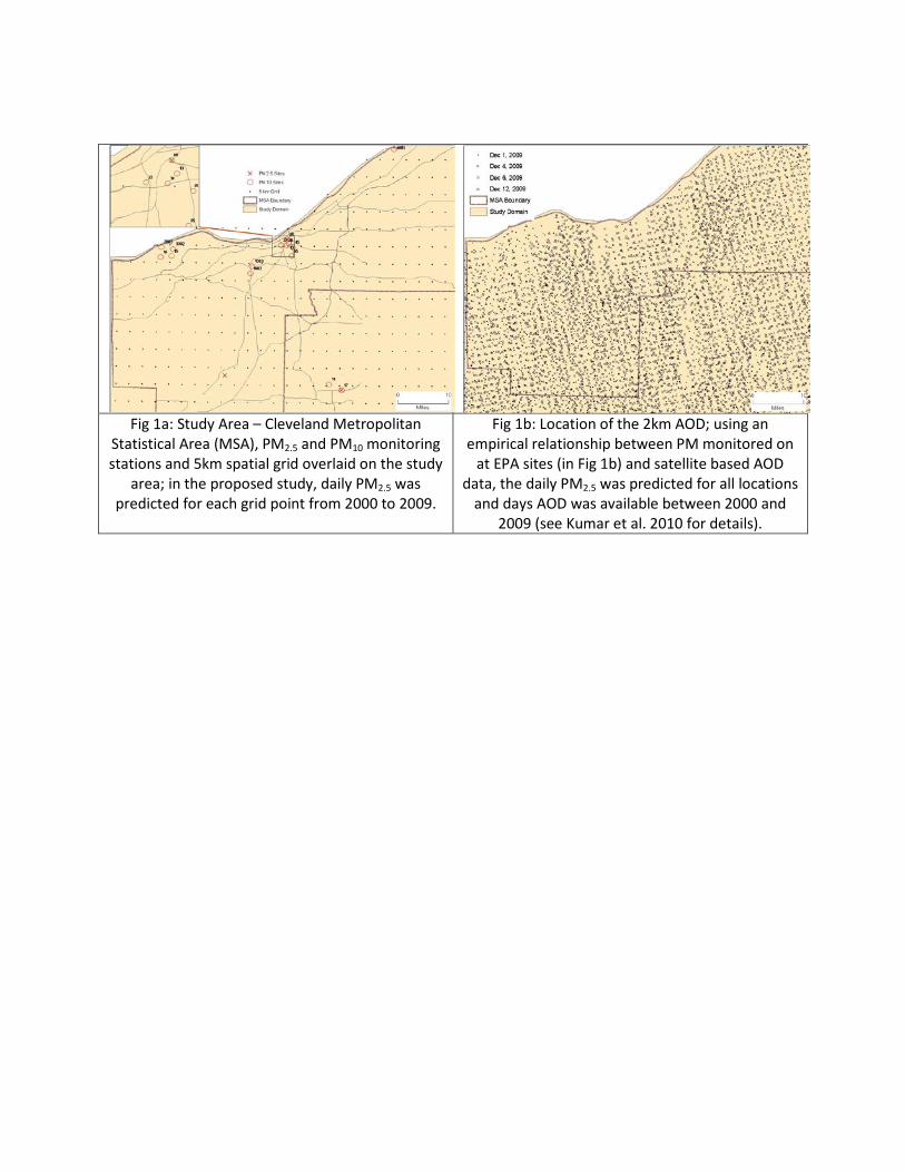
Fig 1a: Study Area – Cleveland Metropolitan
Statistical Area (MSA), PM2.5 and PM10 monitoring stations and 5km spatial grid overlaid on the study
area; in the proposed study, daily PM2.5 was predicted for each grid point from 2000 to 2009.
Fig 1b: Location of the 2km AOD; using an empirical relationship between PM monitored on
at EPA sites (in Fig 1b) and satellite based AOD data, the daily PM2.5 was predicted for all locations
and days AOD was available between 2000 and 2009 (see Kumar et al. 2010 for details).

Fig 2: Time series plot of predicted PM2.5 for a randomly selected site during the study period along with
the observations; scatter plots of PM2.5 for three different time periods.
Local CMP kriging Markov Regional Kriging (grid) Markov Regional Kriging (optimal)
p
redi
cted
5%
n~11
468
10%
n~
229
37
50%
* n
~ 90
65
observed Fig 3: Cross validation plots using the data for 2002 in Cleveland MSA. Using local CMP kriging, Markov regional kriging with 25 by 20 grid or with 568 optimal knots; leaving out 5%, 10% of data and 50% of summer data.
Latitude
Obs
erve
d Da
ta
Loca
l CM
P Kr
igin
g
Mar
kov
Regi
onal
Kr
igin
g
M
arko
v Re
gion
al
Krig
ing
(Opt
imal
)
Longitude
Fig 4: Observed data and predicted values from local CMP kriging, Markov regional kriging with 25 by 20 grid or with 568 optimal knots ; using the data on selected days in summer, fall and winter 2002 for
Cleveland, MSA.
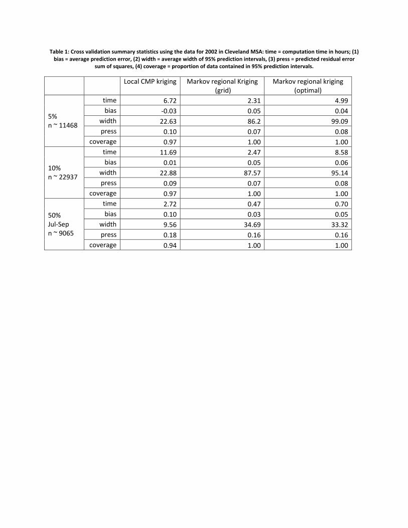
Table 1: Cross validation summary statistics using the data for 2002 in Cleveland MSA: time = computation time in hours; (1) bias = average prediction error, (2) width = average width of 95% prediction intervals, (3) press = predicted residual error
sum of squares, (4) coverage = proportion of data contained in 95% prediction intervals.
Local CMP kriging
Markov regional Kriging (grid)
Markov regional kriging (optimal)
5% n ~ 11468
time 6.72 2.31 4.99 bias -0.03 0.05 0.04
width 22.63 86.2 99.09 press 0.10 0.07 0.08
coverage 0.97 1.00 1.00
10% n ~ 22937
time 11.69 2.47 8.58 bias 0.01 0.05 0.06
width 22.88 87.57 95.14 press 0.09 0.07 0.08
coverage 0.97 1.00 1.00
50% Jul-Sep n ~ 9065
time 2.72 0.47 0.70 bias 0.10 0.03 0.05
width 9.56 34.69 33.32 press 0.18 0.16 0.16
coverage 0.94 1.00 1.00