Tópicos Especiais em Aprendizagem

Reinaldo Bianchi

Centro Universitário da FEI

2012

2a. Aula

Parte B

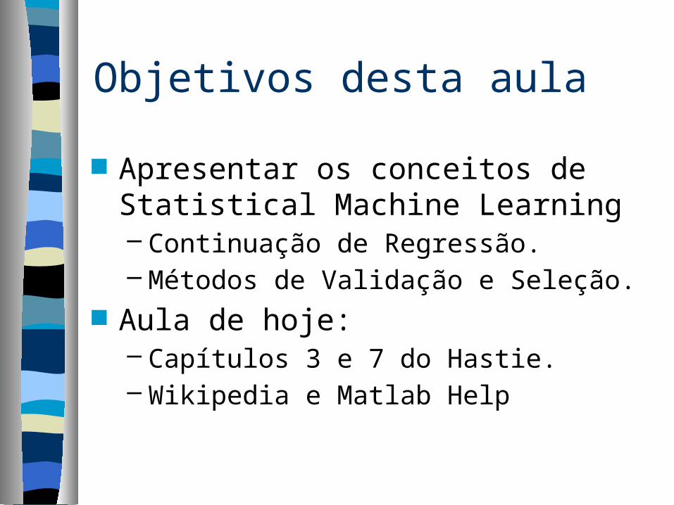
Objetivos desta aula

Apresentar os conceitos de Statistical Machine Learning– Continuação de Regressão.– Métodos de Validação e Seleção.

Aula de hoje: – Capítulos 3 e 7 do Hastie.– Wikipedia e Matlab Help

Métodos de Validação e Seleção

Como ter certeza que o método escolhido é bom?

Capítulo 7 do Hastie

e Wikipedia

5

A Discussion about Linear Regression LMS can be used to determine the least

squared regression equation. The least squared regression method

provides an equation which gives the best linear relationship that exists between the dependent and independent variables.

6

A Discussion about Linear Regression Sometimes, however, the “best”

relationship is not sufficient or reliable enough for estimation.

If you are estimating inventory or other major business decisions, it is very costly to be inaccurate.

Statistics gives various measures for determining whether a regression line is “good” or reliable.

Modelos de Validação e Seleção: Why? “The generalisation performance of a

learning method relates to its prediction capability on independent test data.”

“Assessment of this performance is extremely important in practice, since it guides the choice of learning model, and give us a measure of the quality of the chosen model.”

(Hastie et al.)

We might have in mind 2 goals…

Model Selection:– Estimating the performance of different

models in order to choose the (approximate) best one.

Model Assessment:– Having chosen a final model, estimating its

prediction error (generalisation error) on new data.

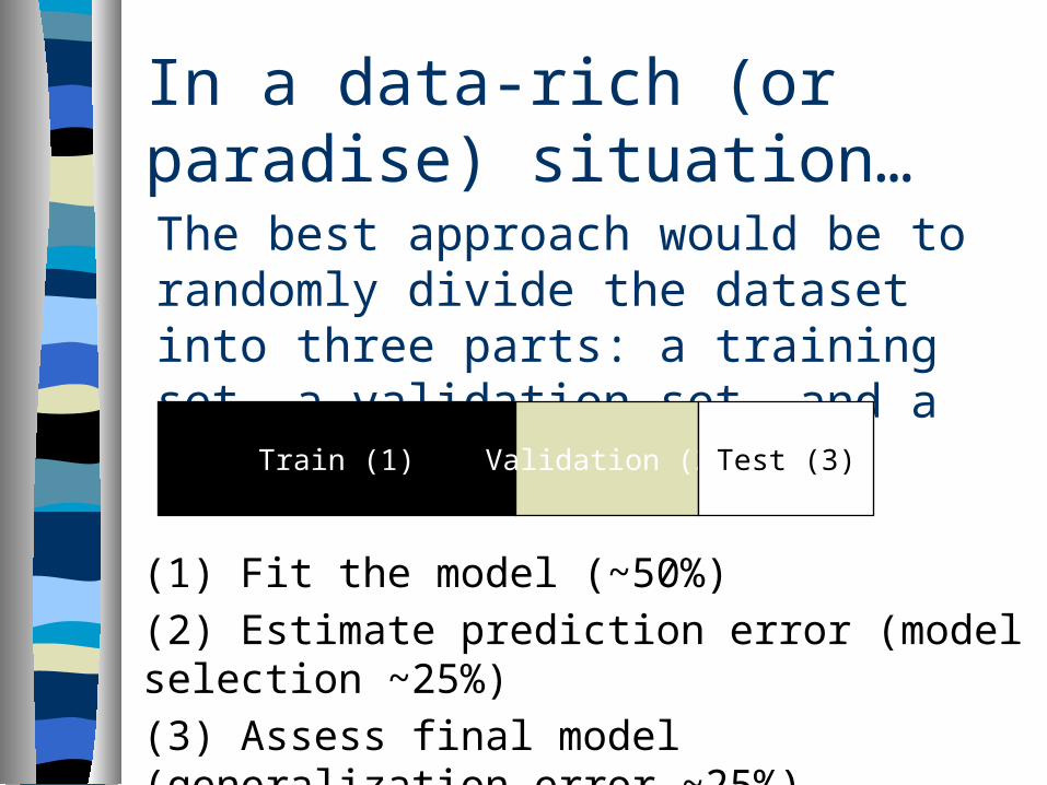
In a data-rich (or paradise) situation… The best approach would be to randomly

divide the dataset into three parts: a training set, a validation set, and a test set.

Train (1) Validation (2) Test (3)

(1) Fit the model (~50%) (2) Estimate prediction error (model selection ~25%) (3) Assess final model (generalization error ~25%)

10

Measures for Evaluating a Regression Line Statistics Provides several Measures for

Determining How Reliable a Line is for Estimation – The Coefficient of Determination, r2.– The Correlation Coefficient, r.– Variance, standard deviation and Z score.– Hypotheses Tests for a Significant

Relationship:• T and Test for the Simple Linear Regression

Model.

11

The Coefficient of Determination, r2

The coefficient of determination gives a value between 0 and 1.

r2 provides the proportion of the total variation in y explained by the simple linear regression model.

The closer this value is to 1 the more reliable the regression line is for estimating y.

12

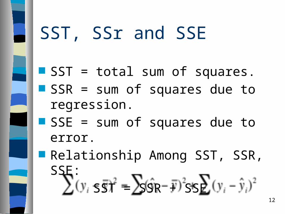
SST, SSr and SSE

SST = total sum of squares. SSR = sum of squares due to

regression. SSE = sum of squares due to error. Relationship Among SST, SSR, SSE:

SST = SSR + SSE

13

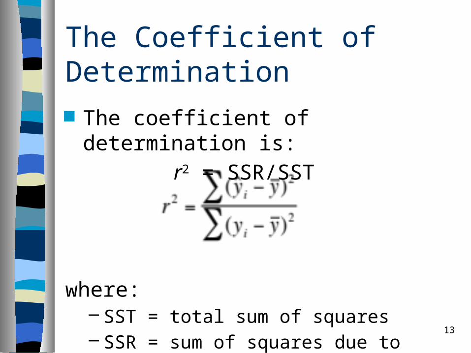
The Coefficient of Determination

The coefficient of determination is:

r2 = SSR/SST

where:– SST = total sum of squares– SSR = sum of squares due to regression

14

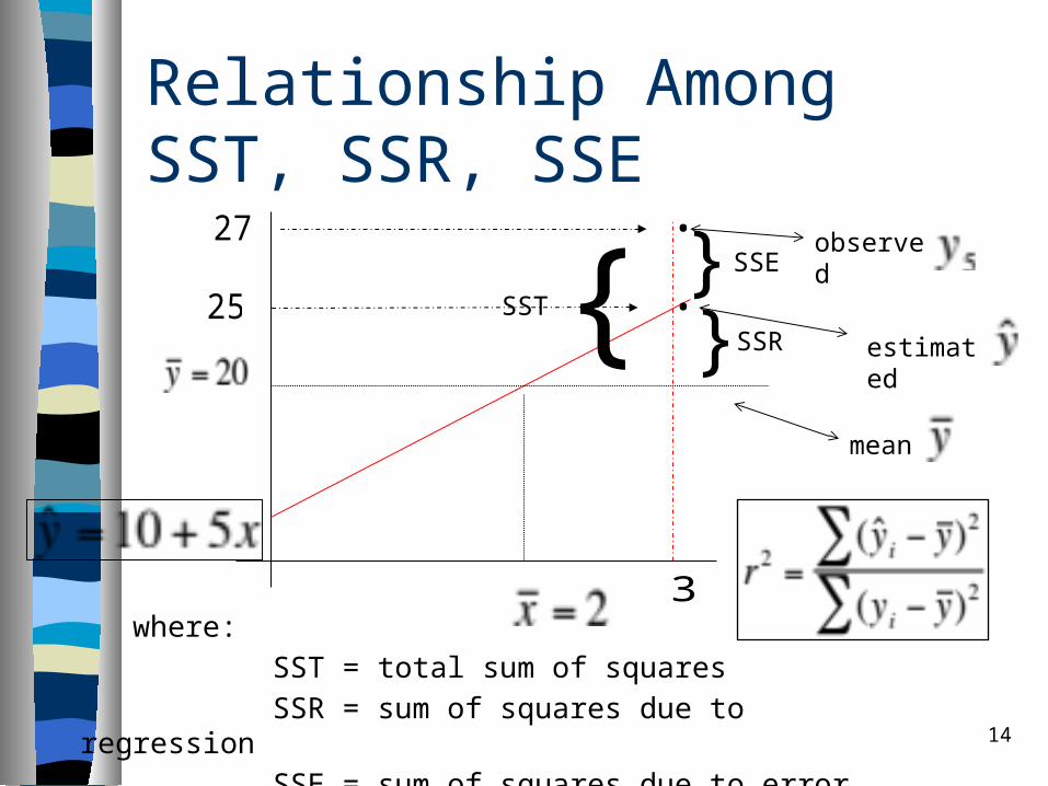
Relationship Among SST, SSR, SSE

where: SST = total sum of squares SSR = sum of squares due to

regression SSE = sum of squares due to error

.25

3

estimated

observed

.27

mean

{SST}}SSR

SSE

15

Example: Reed Auto sales

Reed Auto periodically has a special week-long sale.

As part of the advertising campaign Reed runs one or more television commercials during the weekend preceding the sale.

Data from a sample of 5 previous sales are shown on the next slide.

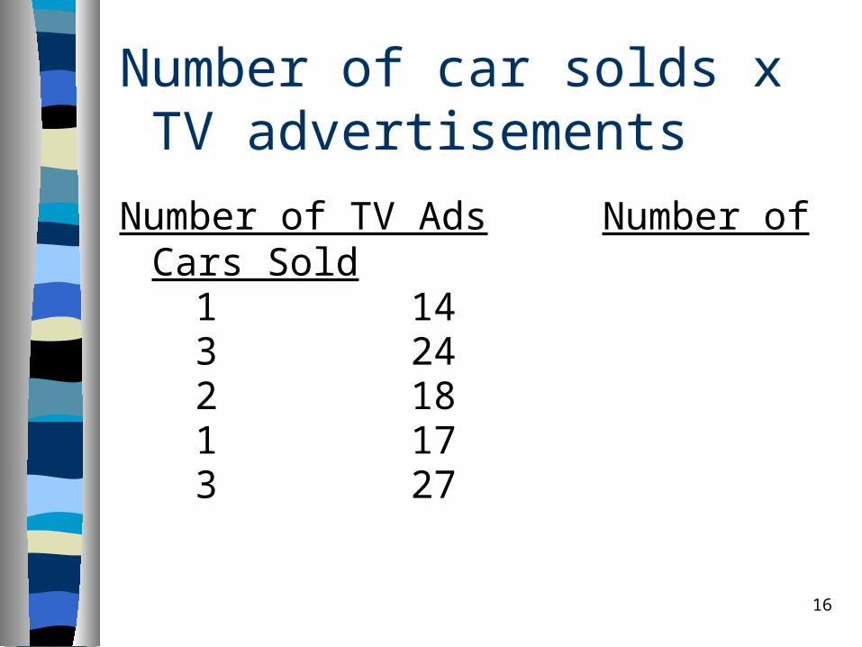
Number of car solds x TV advertisements

Number of TV Ads Number of Cars Sold1 143 242 181 173 27

16

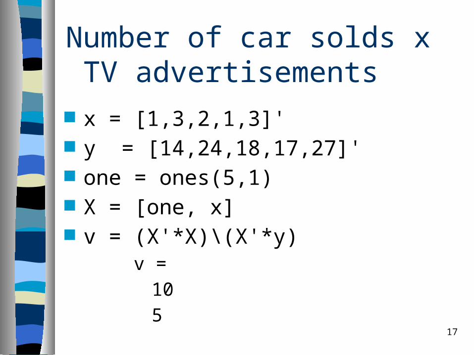
Number of car solds x TV advertisements x = [1,3,2,1,3]' y = [14,24,18,17,27]' one = ones(5,1) X = [one, x] v = (X'*X)\(X'*y)

v =105

17

18

Number of car solds x TV advertisements

19

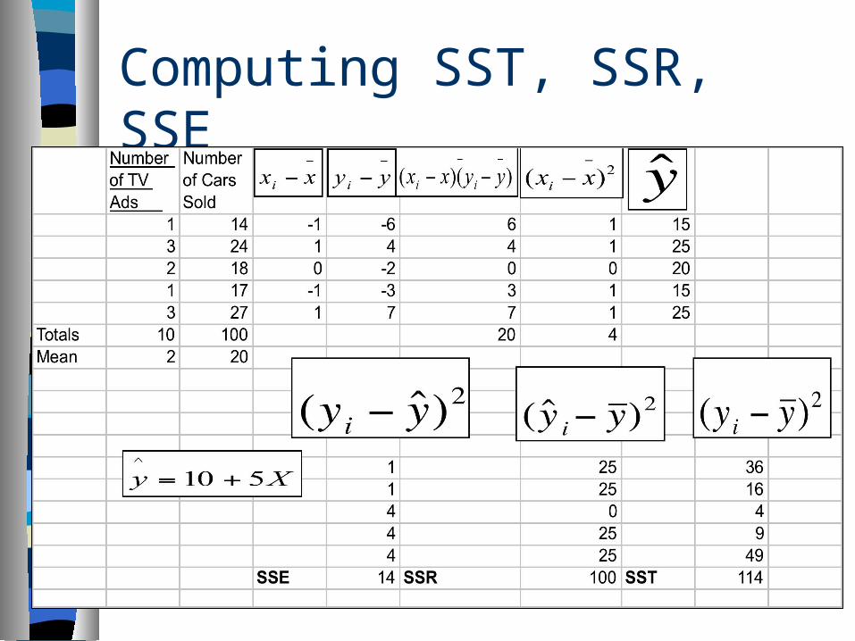
Computing SST, SSR, SSE

20

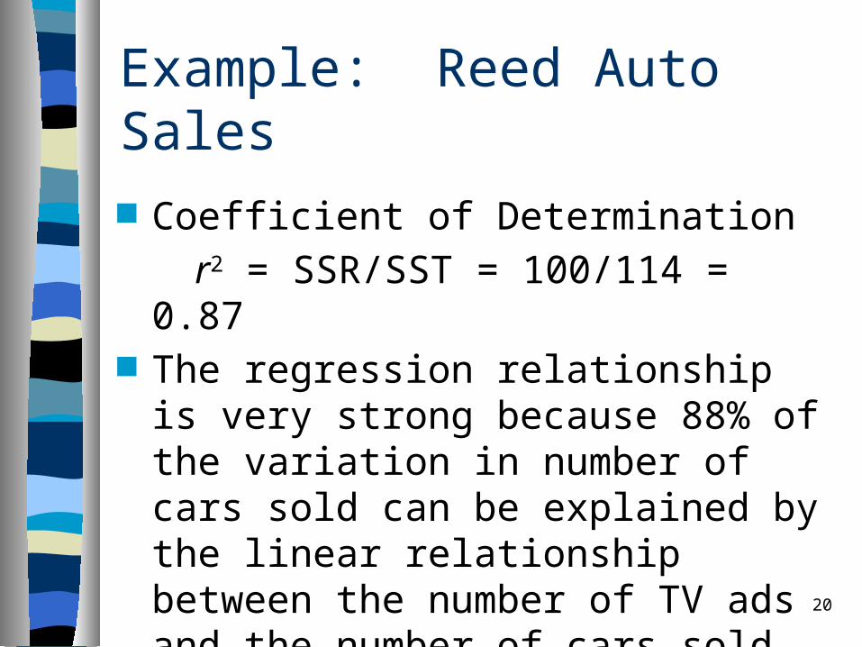
Example: Reed Auto Sales

Coefficient of Determination

r2 = SSR/SST = 100/114 = 0.87

The regression relationship is very strong because 88% of the variation in number of cars sold can be explained by the linear relationship between the number of TV ads and the number of cars sold.

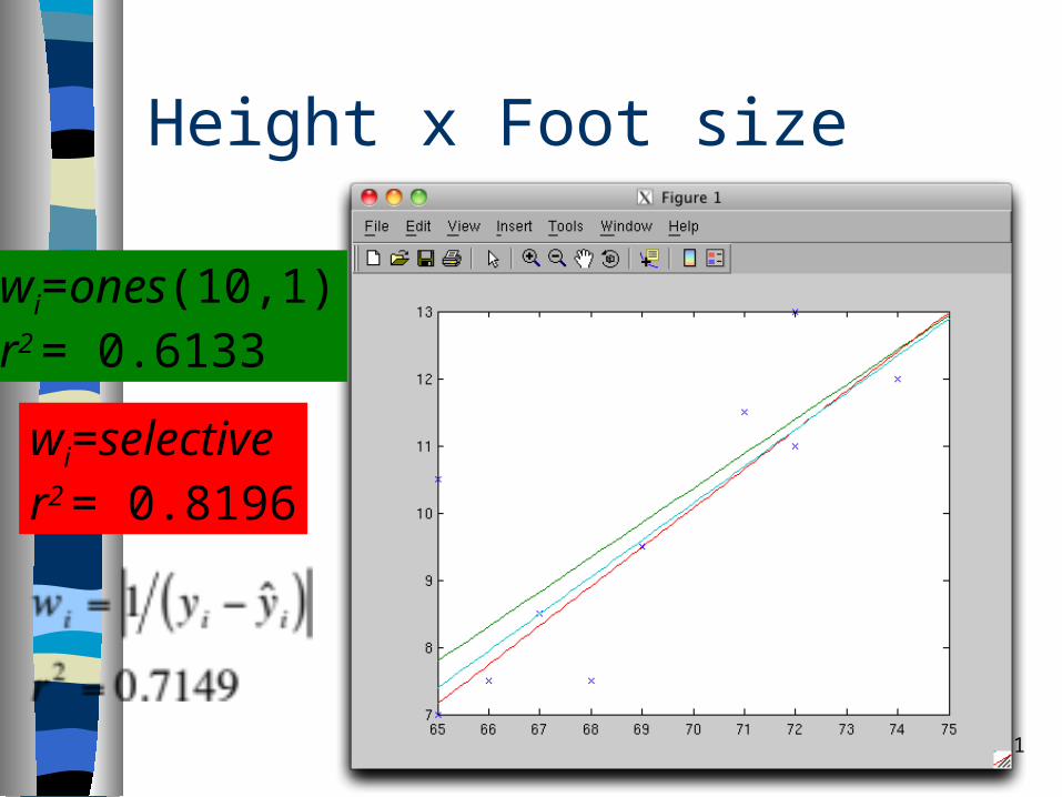
Height x Foot size

21

wi=ones(10,1)r2 = 0.6133

wi=selectiver2 = 0.8196

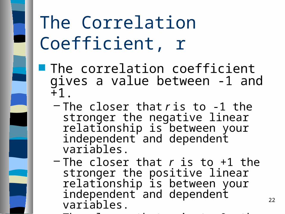
The Correlation Coefficient, r

The correlation coefficient gives a value between -1 and +1.– The closer that r is to -1 the stronger the

negative linear relationship is between your independent and dependent variables.

– The closer that r is to +1 the stronger the positive linear relationship is between your independent and dependent variables.

– The closer that r is to 0, the weaker the linear relationship is between your independent and dependent variables.

22

23

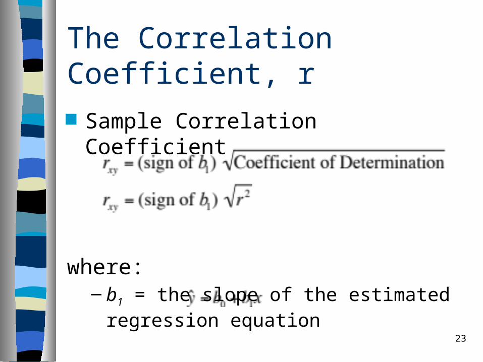
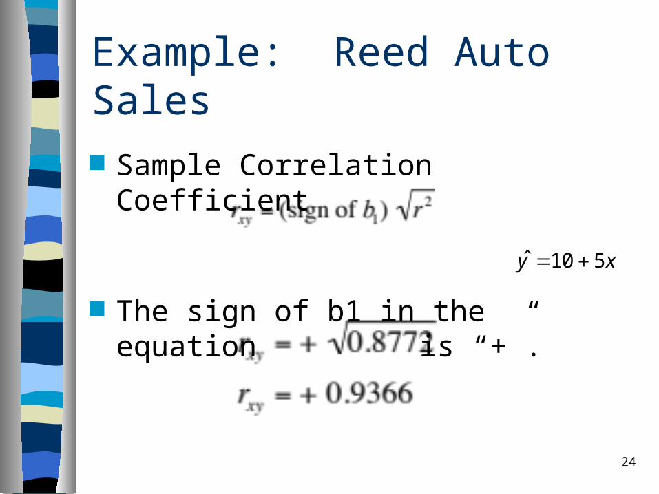
The Correlation Coefficient, r

Sample Correlation Coefficient

where:– b1 = the slope of the estimated regression

equation

24

Example: Reed Auto Sales

Sample Correlation Coefficient

The sign of b1 in the equation is “+”.

ˆ 10 5y x

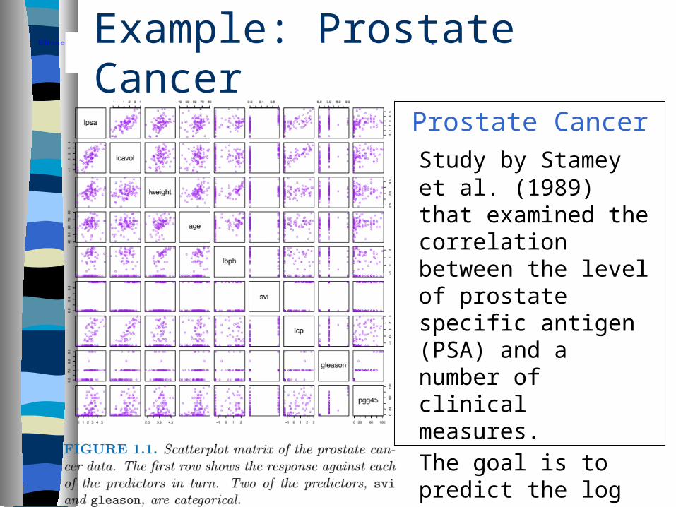
Prostate Cancer

Study by Stamey et al. (1989) that examined the correlation between the level of prostate specific antigen (PSA) and a number of clinical measures.

The goal is to predict the log of PSA (lpsa) from a number of measurements.

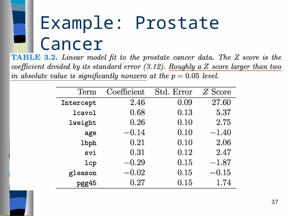
Example: Prostate Cancer

Example: Prostate Cancer

26

Example: Prostate Cancer

27Significant Not Significant

Variance and Standard deviation

Variance - s 2

– is a measure of the amount of variation within the values of that variable, taking account of all possible values and their probabilities or weightings.

Standard deviation - s – is the square root of the variance. – Widely used measure of the variability

28

29

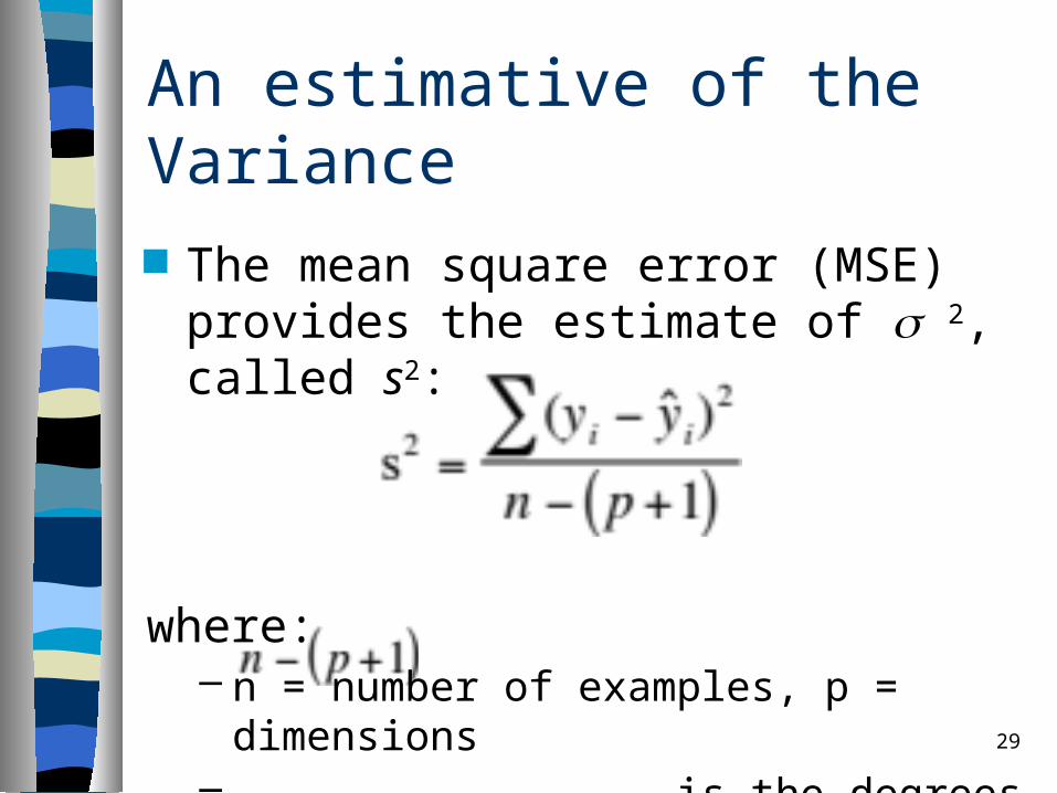
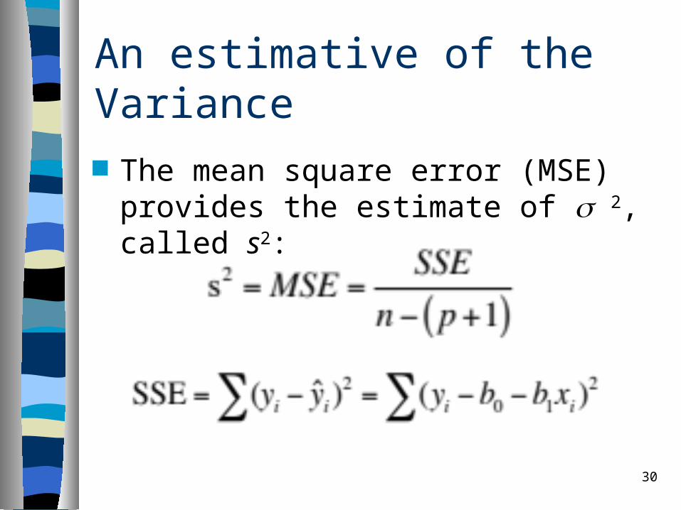
An estimative of the Variance

The mean square error (MSE) provides the estimate of s 2, called s2:

where:– n = number of examples, p = dimensions– is the degrees of freedom.

The estimator s2 is called the sample variance, since it is the variance of the sample (x1, …, xn).

30

An estimative of the Variance

The mean square error (MSE) provides the estimate of s 2, called s2:

31

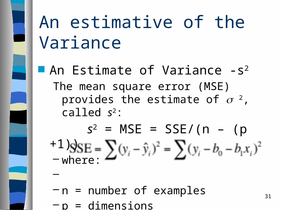
An estimative of the Variance

An Estimate of Variance -s2

The mean square error (MSE) provides the estimate of s 2, called s2:

s2 = MSE = SSE/(n – (p +1))– where:– – n = number of examples– p = dimensions

Degrees of Freedom

In Statistics, degrees of freedom is the number of values in the final calculation of a statistic that are free to vary.

For variance, we use p = dimension

– In Linear Regression is the number of parameters to fit.

32

33

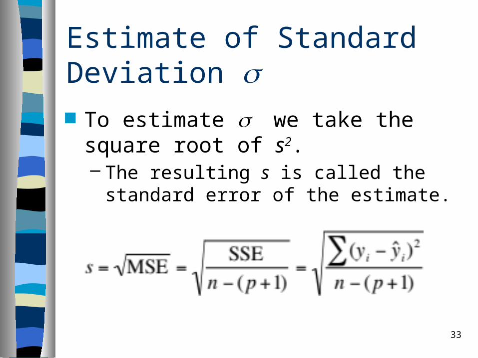
Estimate of Standard Deviation s

To estimate s we take the square root of s2.– The resulting s is called the standard error

of the estimate.

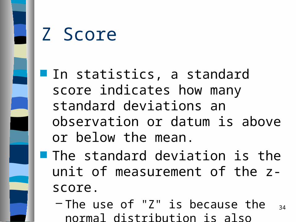
Z Score

In statistics, a standard score indicates how many standard deviations an observation or datum is above or below the mean.

The standard deviation is the unit of measurement of the z-score.– The use of "Z" is because the normal

distribution is also known as the "Z distribution"

34

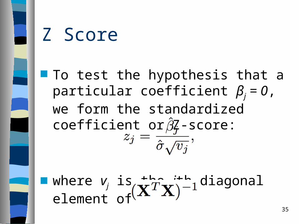
Z Score

To test the hypothesis that a particular coefficient βj = 0, we form the standardized coefficient or Z-score:

where vj is the jth diagonal element of

35

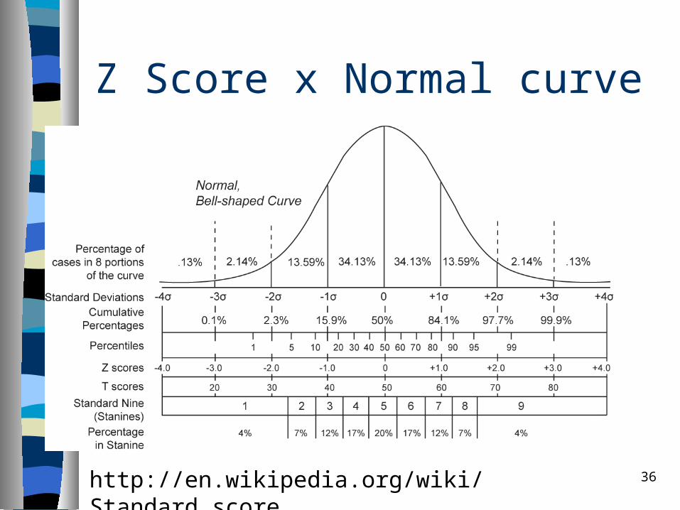
Z Score x Normal curve

36http://en.wikipedia.org/wiki/Standard_score

Example: Prostate Cancer

37

38

Testing for Significance

To test for a significant regression relationship, we must conduct a hypothesis test to determine whether the value of b1 is zero.

Two tests are commonly used– t Test– F Test

All require an estimate of s 2, the variance of e in the regression model.

39

Testing for Significance: Student t-Test A t-test is a statistical hypothesis test in

which the test statistic follows a Student's t distribution if the null hypothesis is supported:– The null hypothesis H0 proposes a general

or default position, such as that there is no relationship between two measured phenomena, or that a potential treatment has no effect.

40

Testing for Significance: Students t-Test The t-test assesses whether the means

of two groups are statistically different from each other.

If they are, a second hypothesis is valid:– The alternative hypothesis Ha , which

asserts a particular relationship between the phenomena.

History

The t-test was introduced in 1908 by William Sealy Gosset, a chemist working for the Guinness brewery ("Student" was his pen name).– Gosset had been hired due to Claude

Guinness's innovative policy of recruiting the best graduates from Oxford and Cambridge to apply biochemistry and statistics to Guinness' industrial processes.

41

42

Computing t

Usually, t = Z/s

where:–Z is designed to be sensitive to the

alternative hypothesis:• Its magnitude tends to be larger when the

alternative hypothesis is true

– s is a scaling parameter that allows the distribution of T to be determined.

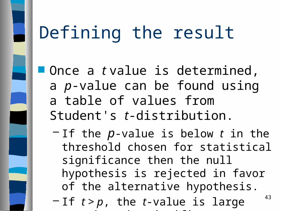
Defining the result

Once a t value is determined, a p-value can be found using a table of values from Student's t-distribution. – If the p-value is below t in the threshold

chosen for statistical significance then the null hypothesis is rejected in favor of the alternative hypothesis.

– If t > p, the t-value is large enough to be significant.

43

44

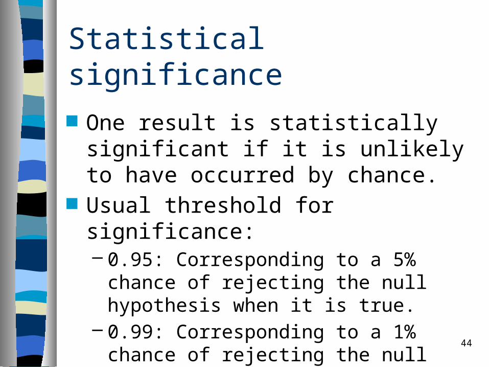
Statistical significance

One result is statistically significant if it is unlikely to have occurred by chance.

Usual threshold for significance:– 0.95: Corresponding to a 5% chance of

rejecting the null hypothesis when it is true.– 0.99: Corresponding to a 1% chance of

rejecting the null hypothesis when it is true.– 0.995: Corresponding to a 0.5% chance of

rejecting the null hypothesis when it is true.

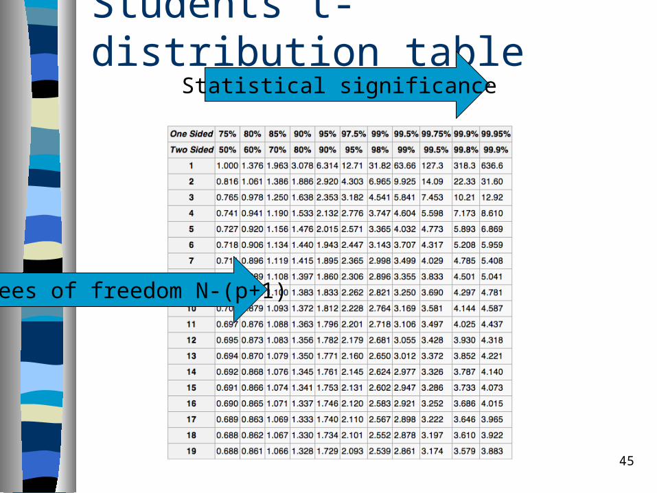
Students t-distribution table

45

Statistical significance

Degre

es o

f freed

om

N-(p

+1

)

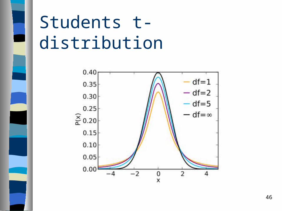
Students t-distribution

46

47

Example: Independent one-sample t-test In testing the null hypothesis that the

population mean is equal to a specified value μ0, one uses the statistic:

where:– is the mean value of xi.

– μ0 is the value to test.– s is the standart deviation.

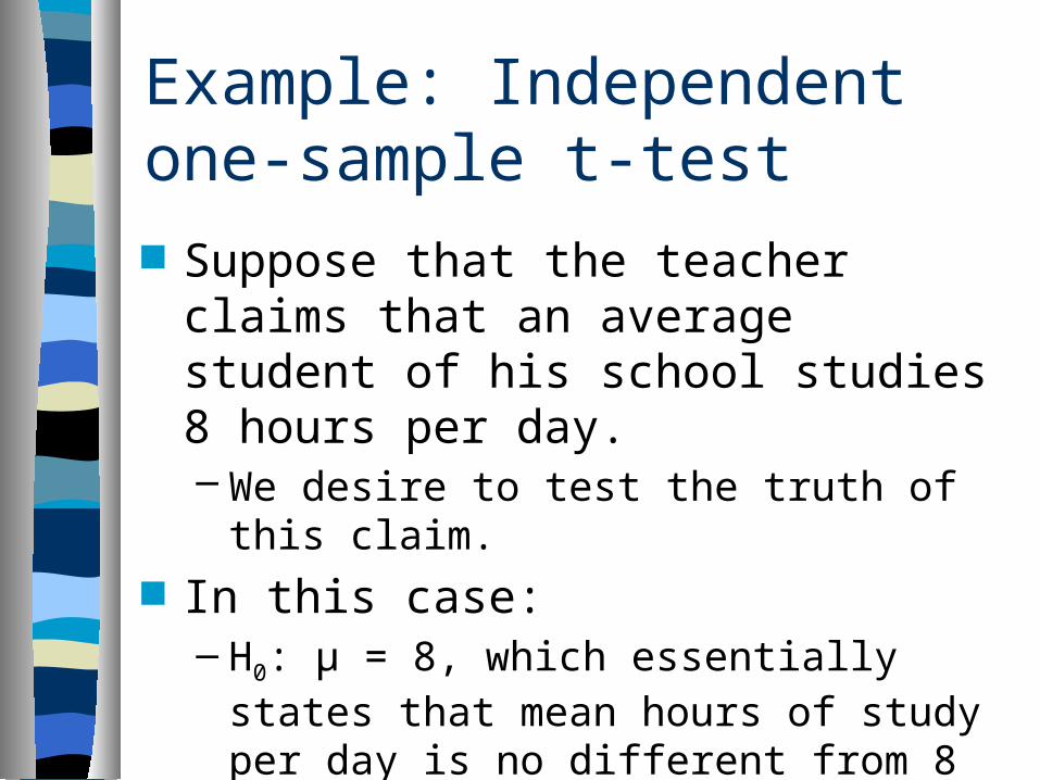
Example: Independent one-sample t-test Suppose that the teacher claims that an

average student of his school studies 8 hours per day.– We desire to test the truth of this claim.

In this case:– H0: μ = 8, which essentially states that

mean hours of study per day is no different from 8 hours.

– Ha: μ ≠ 8, which is negation of the claim.

Example: Independent one-sample t-test Data from 10 students:

– X = [5,6,7,3,5,9,9,2,3,10] Computing t:

– Mean = 5.90– Sample standart deviation = 2.807– t = - 2.3660.

Using matlab: – t = (mean (X)-8)/(std(X)/sqrt(10))

49

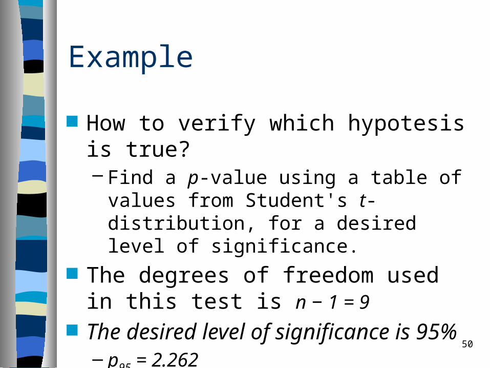
Example

How to verify which hypotesis is true?– Find a p-value using a table of values from

Student's t-distribution, for a desired level of significance.

The degrees of freedom used in this test is n − 1 = 9

The desired level of significance is 95%– p95 = 2.262

50

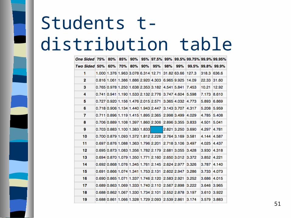
Students t-distribution table

51

52

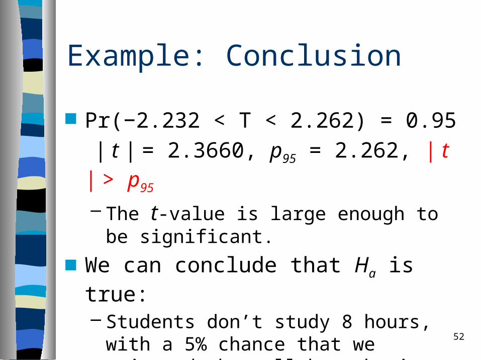
Example: Conclusion

Pr(−2.232 < T < 2.262) = 0.95

| t | = 2.3660, p95 = 2.262, | t | > p95

– The t-value is large enough to be significant.

We can conclude that Ha is true:– Students don’t study 8 hours, with a 5%

chance that we rejected the null hypothesis when it is true.

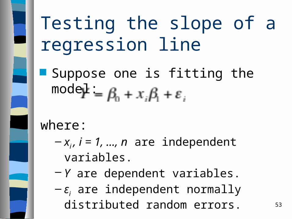
Testing the slope of a regression line Suppose one is fitting the model:

where:– xi , i = 1, ..., n are independent variables.

– Y are dependent variables.– εi are independent normally distributed

random errors.

53

Testing the slope of a regression line It is desired to test the null hypothesis,

that the slope computed using LMS β1 is equal to some specified value:– If β1 = 0, the hypothesis is that x and y are

unrelated because the angle of the slope is zero.

– Therefore, Z = β1 – 0.

54

55

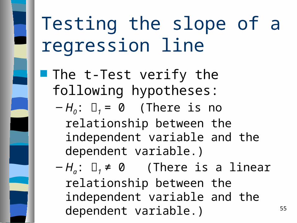
Testing the slope of a regression line The t-Test verify the following

hypotheses:– H0: 1 = 0 (There is no relationship

between the independent variable and the dependent variable.)

– Ha: 1 ≠ 0 (There is a linear relationship between the independent variable and the dependent variable.)

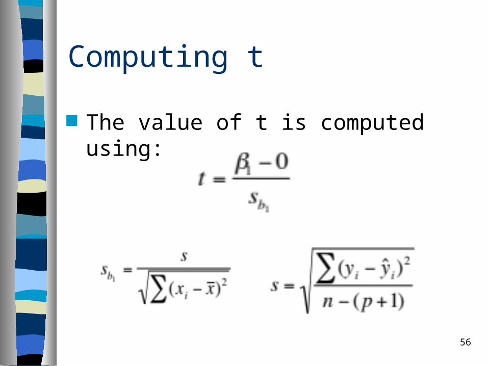
Computing t

The value of t is computed using:

56

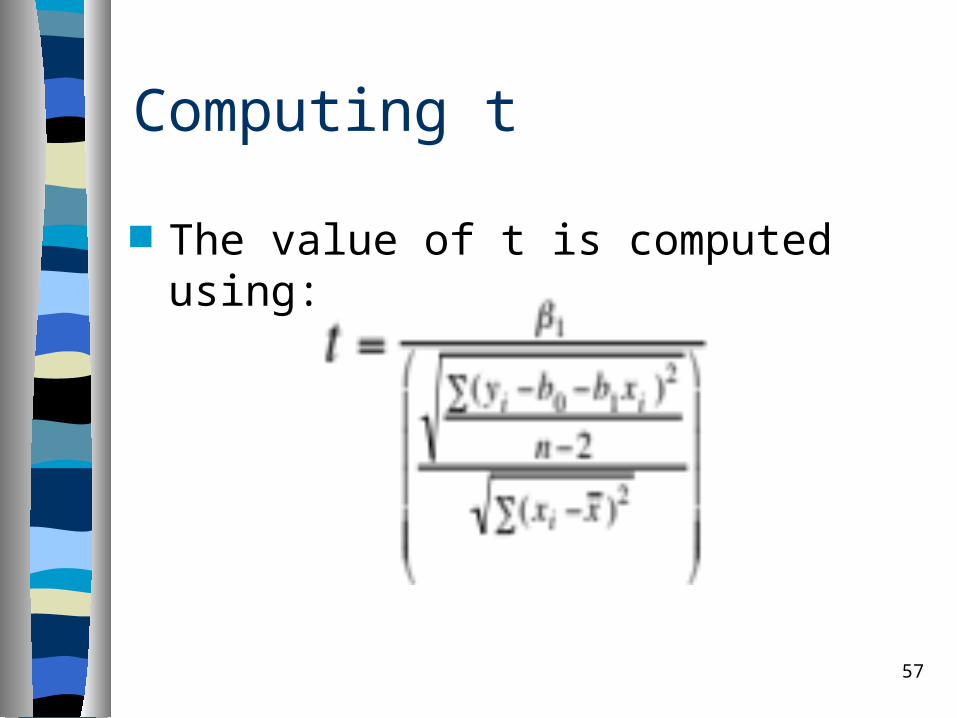
Computing t

The value of t is computed using:

57

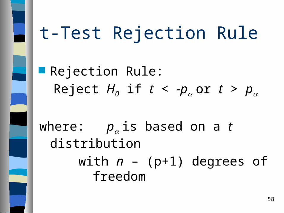
t-Test Rejection Rule

Rejection Rule:

Reject H0 if t < -por t > p

where: p is based on a t distribution

with n – (p+1) degrees of freedom

58

59

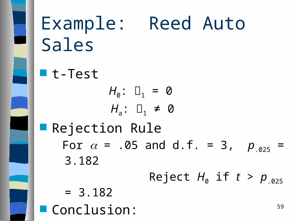
Example: Reed Auto Sales

t-Test H0: 1 = 0

Ha: 1 ≠ 0

Rejection Rule For = .05 and d.f. = 3, p.025 = 3.182

Reject H0 if t > p.025 = 3.182

Conclusion:– t = 4.63 > 3.182, so reject H0

– There is a relation between ads and sales.

60

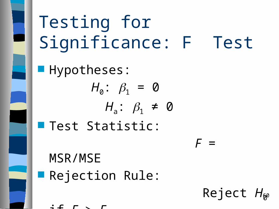
Testing for Significance: F Test

Hypotheses:

H0: 1 = 0

Ha: 1 ≠ 0 Test Statistic:

F = MSR/MSE Rejection Rule: Reject H0 if F > F

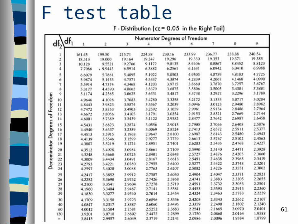
F test table

61

62

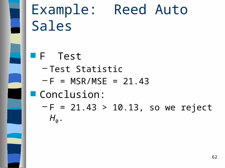
Example: Reed Auto Sales

F Test– Test Statistic– F = MSR/MSE = 21.43

Conclusion:– F = 21.43 > 10.13, so we reject H0.

63

ANOVA (analysis of variance)

ANOVA provides a statistical test of whether or not the means of several groups are all equal, and therefore generalizes t-test to more than two groups. – Doing multiple two-sample t-tests would

result in an increased chance of committing a type I error.

– For this reason, ANOVAs are useful in comparing two, three, or more means.

ANOVA

The standard ANOVA test divides the variability of the data into two parts:– Variability due to the differences among the

column means (variability between groups).

– Variability due to the differences between the data in each column and the column mean (variability within groups).

64

ANOVA

The usual ANOVA table has six columns:– The source of the variability.– The sum of squares (SS) due to each

source.– The degrees of freedom (df) associated with

each source.– The mean squares (MS) for each source,

which is the ratio SS/df.– The F-statistic.– The p-value.

65

66

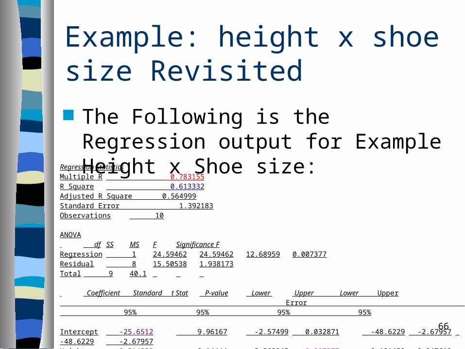
Example: height x shoe size Revisited

SUMMARY OUTPUT

Regression StatisticsMultiple R 0.783155

R Square 0.613332

Adjusted R Square 0.564999

Standard Error 1.392183

Observations 10

ANOVA  df SS MS F Significance FRegression 1 24.59462 24.59462 12.68959 0.007377Residual 8 15.50538 1.938173Total 9 40.1      

  Coefficient Standard t Stat P-value Lower Upper Lower Upper Error 95% 95% 95% 95%

Intercept -25.6512 9.96167 -2.57499 0.032871 -48.6229 -2.67957 -48.6229 -2.67957Height, x 0.514532 0.14444 3.562245 0.007377 0.181452 0.847612 0.181452 0.847612

The Following is the Regression output for Example Height x Shoe size:

67

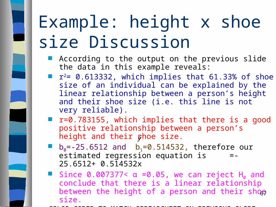
According to the output on the previous slide the data in this example reveals:

r2= 0.613332, which implies that 61.33% of shoe size of an individual can be explained by the linear relationship between a person’s height and their shoe size (i.e. this line is not very reliable).

r=0.783155, which implies that there is a good positive relationship between a person’s height and their shoe size.

b0=-25.6512 and b1=0.514532, therefore our estimated regression equation is =-25.6512+ 0.514532x

Since 0.007377< α =0.05, we can reject H0 and conclude that there is a linear relationship between the height of a person and their shoe size.

COLOR CODED TO MATCH SPREADSHEET ON PREVIOUS SLIDE

Example: height x shoe size Discussion

y

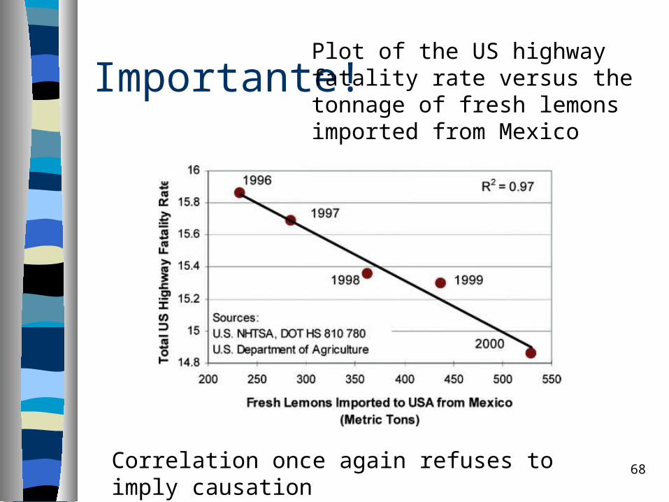
Importante!

68

Plot of the US highway fatality rate versus the tonnage of fresh lemons imported from Mexico

Correlation once again refuses to imply causation

E no Matlab?

69

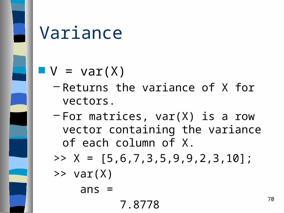
Variance

V = var(X) – Returns the variance of X for vectors. – For matrices, var(X) is a row vector

containing the variance of each column of X.

>> X = [5,6,7,3,5,9,9,2,3,10];>> var(X) ans = 7.8778

70

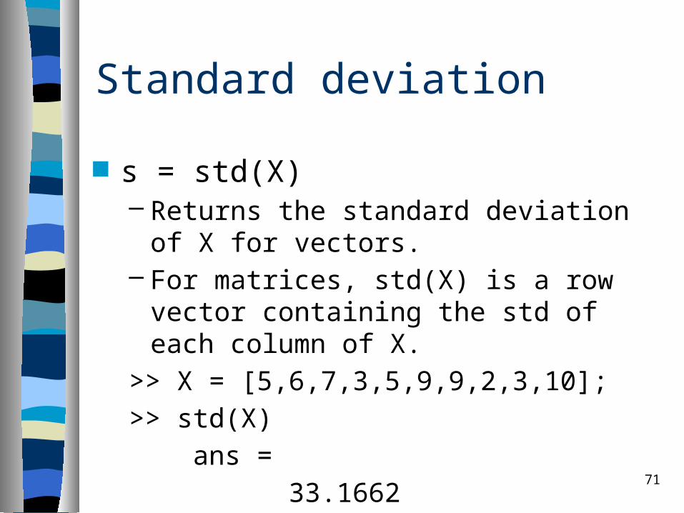
Standard deviation

s = std(X) – Returns the standard deviation of X for

vectors. – For matrices, std(X) is a row vector

containing the std of each column of X.

>> X = [5,6,7,3,5,9,9,2,3,10];>> std(X) ans = 33.1662

71

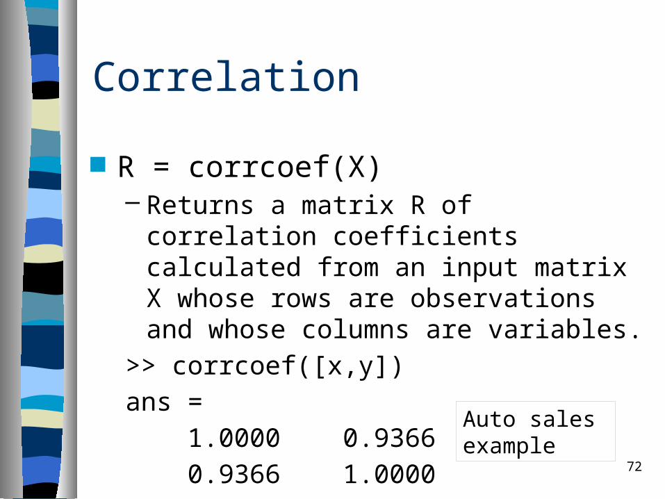
Correlation

R = corrcoef(X)– Returns a matrix R of correlation

coefficients calculated from an input matrix X whose rows are observations and whose columns are variables.

>> corrcoef([x,y])ans = 1.0000 0.9366 0.9366 1.0000

72

Auto sales example

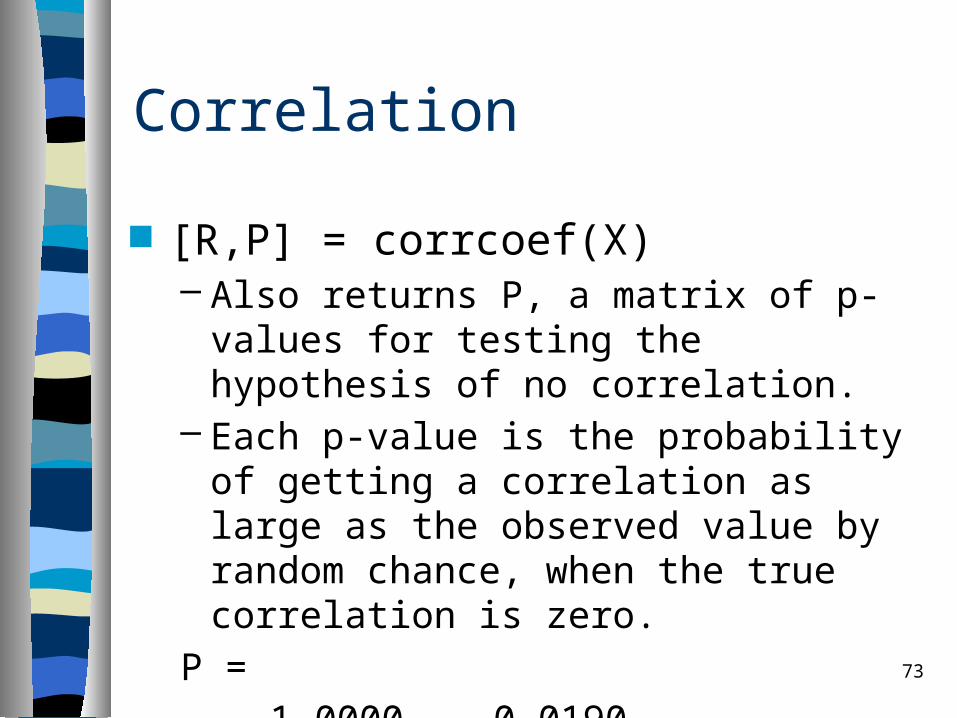
Correlation

[R,P] = corrcoef(X)– Also returns P, a matrix of p-values for

testing the hypothesis of no correlation.– Each p-value is the probability of getting a

correlation as large as the observed value by random chance, when the true correlation is zero.

P = 1.0000 0.0190 0.0190 1.0000 73

74

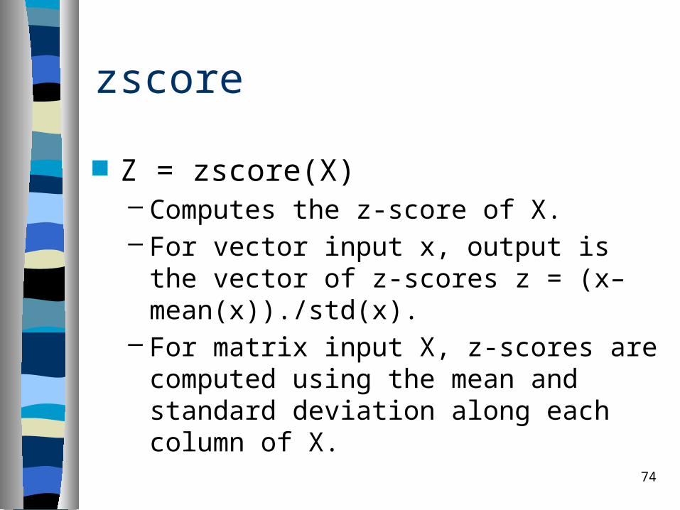
zscore

Z = zscore(X) – Computes the z-score of X.– For vector input x, output is the vector of z-

scores z = (x–mean(x))./std(x). – For matrix input X, z-scores are computed

using the mean and standard deviation along each column of X.

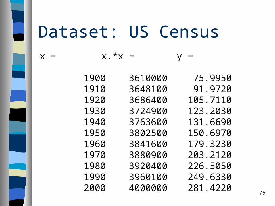
Dataset: US Census

75

x =

1900 1910 1920 1930 1940 1950 1960 1970 1980 1990 2000

y =

75.9950 91.9720 105.7110 123.2030 131.6690 150.6970 179.3230 203.2120 226.5050 249.6330 281.4220

x.*x =

3610000 3648100 3686400 3724900 3763600 3802500 3841600 3880900 3920400 3960100 4000000

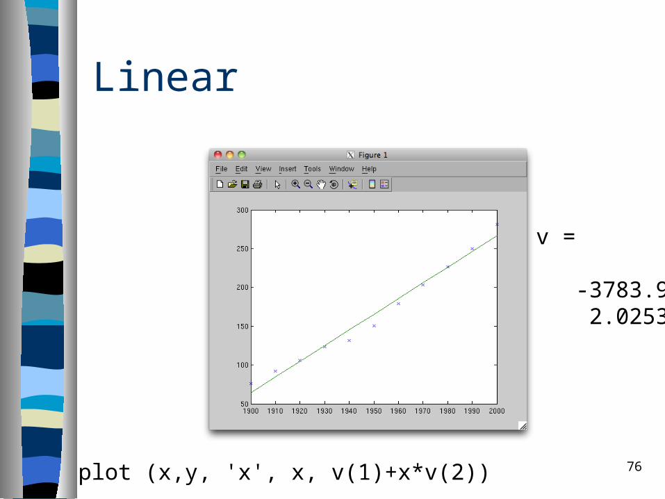
Linear

76

v =

-3783.9 2.0253

plot (x,y, 'x', x, v(1)+x*v(2))

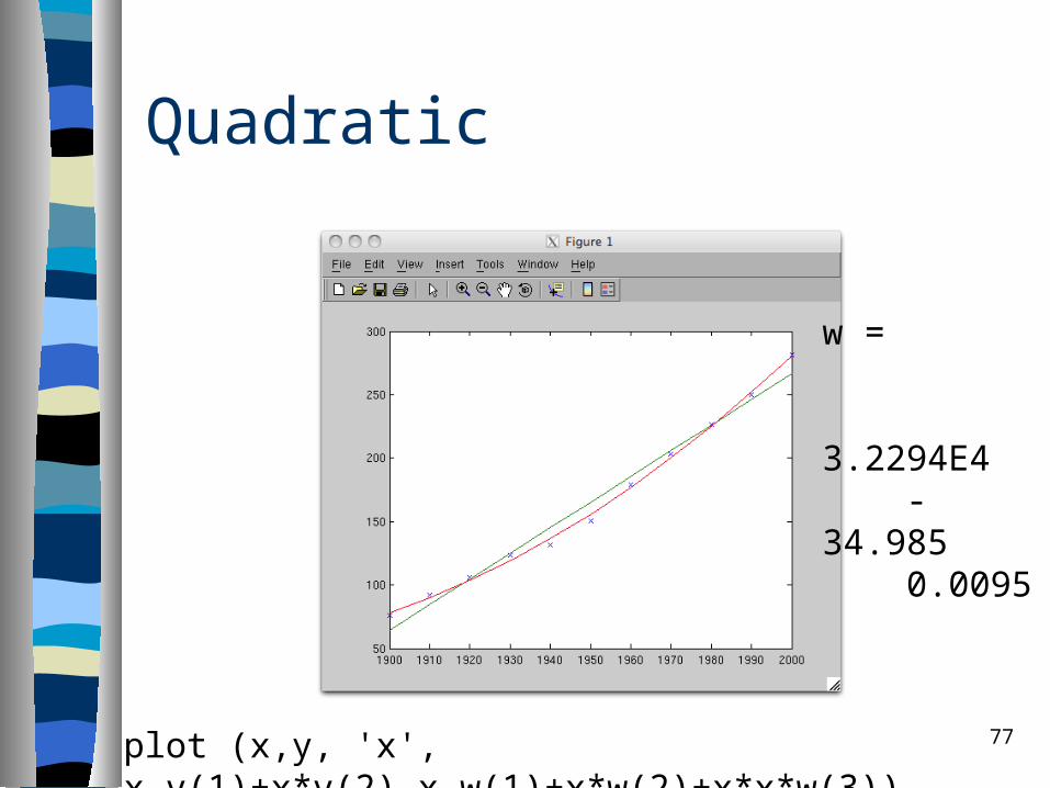
Quadratic

77

w =

3.2294E4 -34.985 0.0095

plot (x,y, 'x', x,v(1)+x*v(2),x,w(1)+x*w(2)+x*x*w(3))

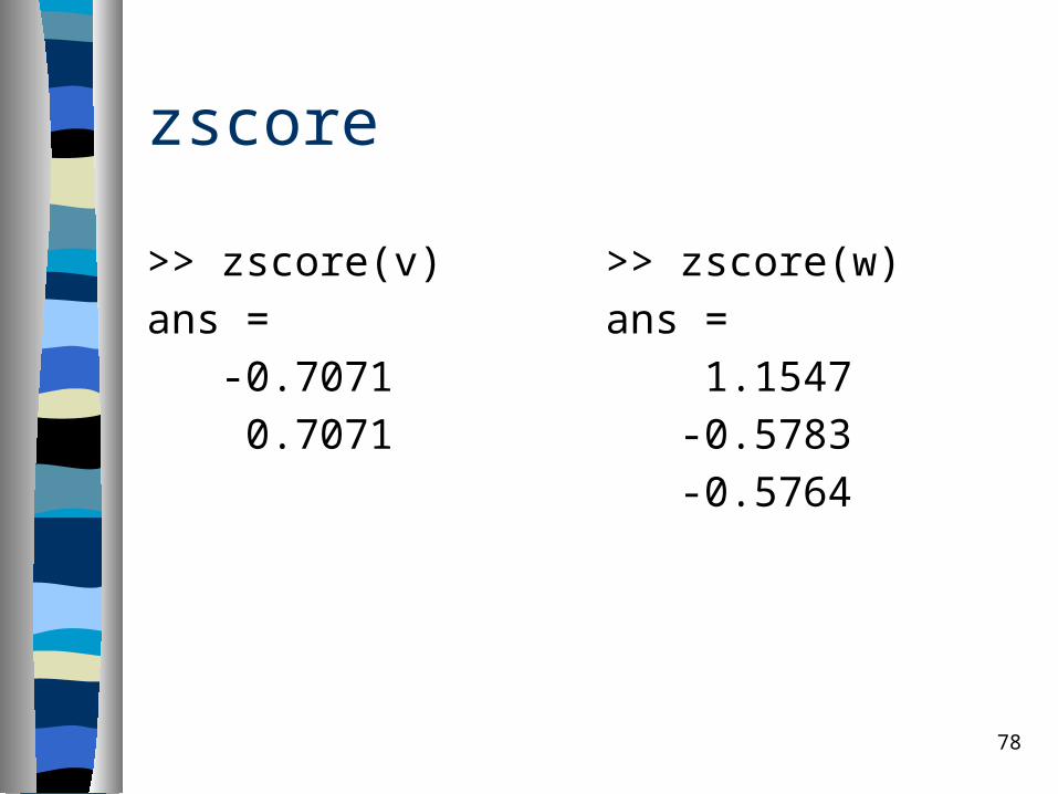
zscore

>> zscore(v)ans = -0.7071 0.7071

>> zscore(w) ans = 1.1547 -0.5783 -0.5764

78

79

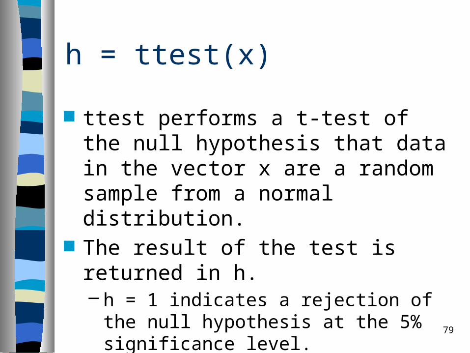
h = ttest(x)

ttest performs a t-test of the null hypothesis that data in the vector x are a random sample from a normal distribution.

The result of the test is returned in h. – h = 1 indicates a rejection of the null

hypothesis at the 5% significance level. – h = 0 indicates a failure to reject the null

hypothesis.

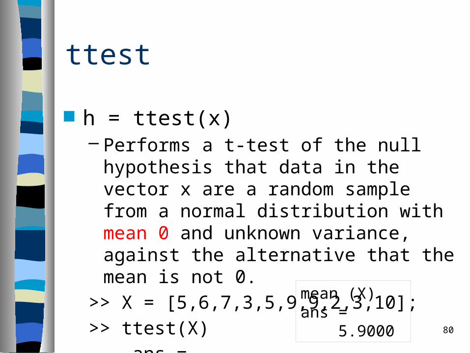
ttest

h = ttest(x)– Performs a t-test of the null hypothesis that

data in the vector x are a random sample from a normal distribution with mean 0 and unknown variance, against the alternative that the mean is not 0.

>> X = [5,6,7,3,5,9,9,2,3,10];>> ttest(X) ans = 1 80

mean (X)ans = 5.9000

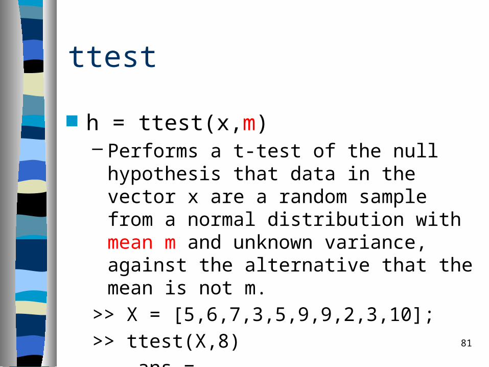
ttest

h = ttest(x,m)– Performs a t-test of the null hypothesis that

data in the vector x are a random sample from a normal distribution with mean m and unknown variance, against the alternative that the mean is not m.

>> X = [5,6,7,3,5,9,9,2,3,10];>> ttest(X,8) ans = 1 81

ttest

h = ttest(x,m)– Performs a t-test of the null hypothesis that

data in the vector x are a random sample from a normal distribution with mean m and unknown variance, against the alternative that the mean is not m.

>> X = [5,6,7,3,5,9,9,2,3,10];>> ttest(X,6) ans = 0 82

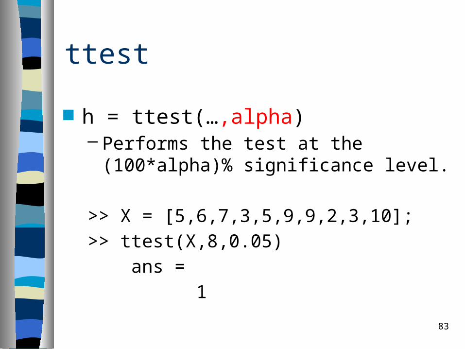
ttest

h = ttest(…,alpha)– Performs the test at the (100*alpha)%

significance level.

>> X = [5,6,7,3,5,9,9,2,3,10];>> ttest(X,8,0.05) ans = 1

83

ttest

h = ttest(…,alpha)– Performs the test at the (100*alpha)%

significance level.

>> X = [5,6,7,3,5,9,9,2,3,10];>> ttest(X,8,0.01) ans = 0

84

ttest2

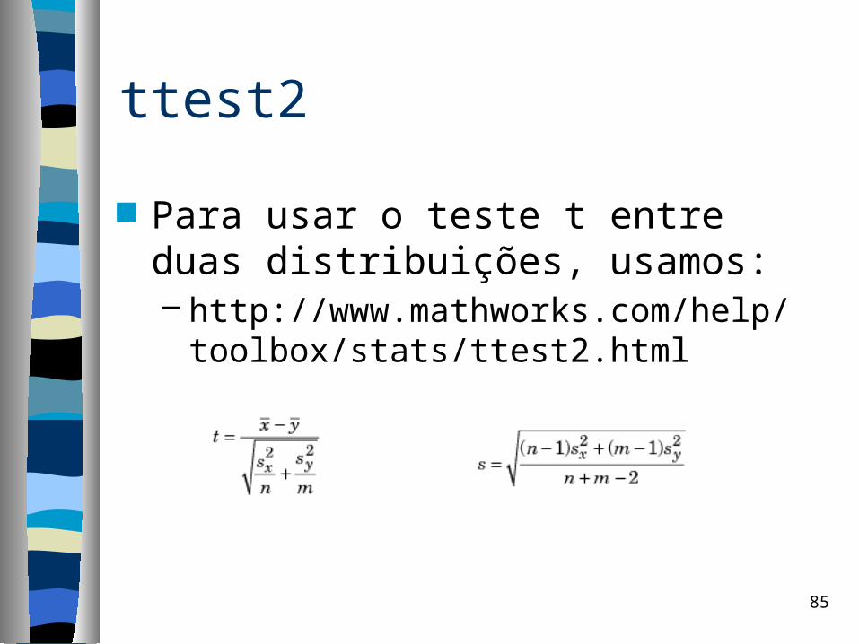
Para usar o teste t entre duas distribuições, usamos:– http://www.mathworks.com/help/toolbox/

stats/ttest2.html

85

86

vartest2

H = vartest2(X,Y)– Performs an F test of the hypothesis that

two independent samples, in the vectors X and Y, come from normal distributions with the same variance, against the alternative that they come from normal distributions with different variances.

– The result is H = 0 if the null hypothesis cannot be rejected or H = 1 if the null hypothesis can be rejected.

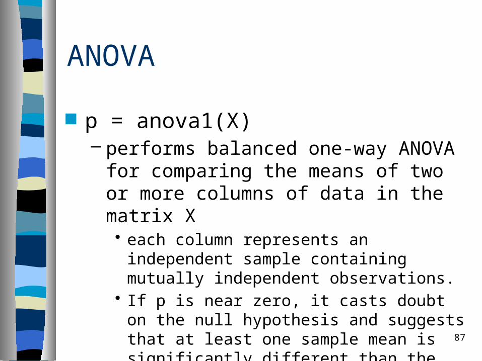
ANOVA

p = anova1(X)– performs balanced one-way ANOVA for

comparing the means of two or more columns of data in the matrix X• each column represents an independent

sample containing mutually independent observations.

• If p is near zero, it casts doubt on the null hypothesis and suggests that at least one sample mean is significantly different than the other sample means. 87

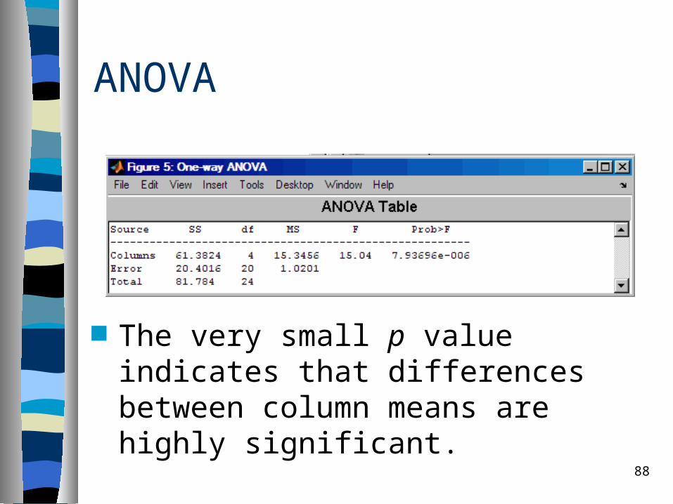
ANOVA

The very small p value indicates that differences between column means are highly significant.

88

89

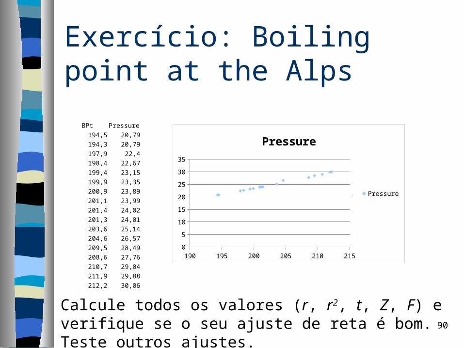
Exercício: Boiling point at the Alps Description: The boiling point of water at

different barometric pressures. There are 17 observations. Variables:

– BPt: the recorded boiling point of water in degrees F

– Pressure: the barometric pressure in inches of mercury.

90

Exercício: Boiling point at the Alps

BPt Pressure194,5 20,79194,3 20,79197,9 22,4198,4 22,67199,4 23,15199,9 23,35200,9 23,89201,1 23,99201,4 24,02201,3 24,01203,6 25,14204,6 26,57209,5 28,49208,6 27,76210,7 29,04211,9 29,88212,2 30,06

190 195 200 205 210 2150

5

10

15

20

25

30

35

Pressure

Pressure

Calcule todos os valores (r, r2, t, Z, F) e verifique se o seu ajuste de reta é bom. Teste outros ajustes.

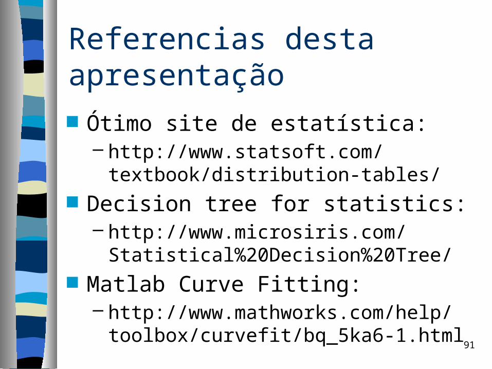
Referencias desta apresentação

Ótimo site de estatística:– http://www.statsoft.com/textbook/

distribution-tables/ Decision tree for statistics:

– http://www.microsiris.com/Statistical%20Decision%20Tree/

Matlab Curve Fitting:– http://www.mathworks.com/help/toolbox/

curvefit/bq_5ka6-1.html91

Conclusão

Vimos um pouco mais sobre regressão:– Métodos Robustos– Métodos de Seleção.

Vimos modelos de avaliação da qualidade de um ajuste de função:– Valores r, r2, Z– Testes T, e F

92

Terminando:

CERN experiments observe particle consistent with long-sought Higgs boson:– “We observe in our data clear signs of a

new particle, at the level of 5 sigma, in the mass region around 126 GeV.” said ATLAS experiment spokesperson Fabiola Gianotti, “but a little more time is needed to prepare these results for publication.”

93

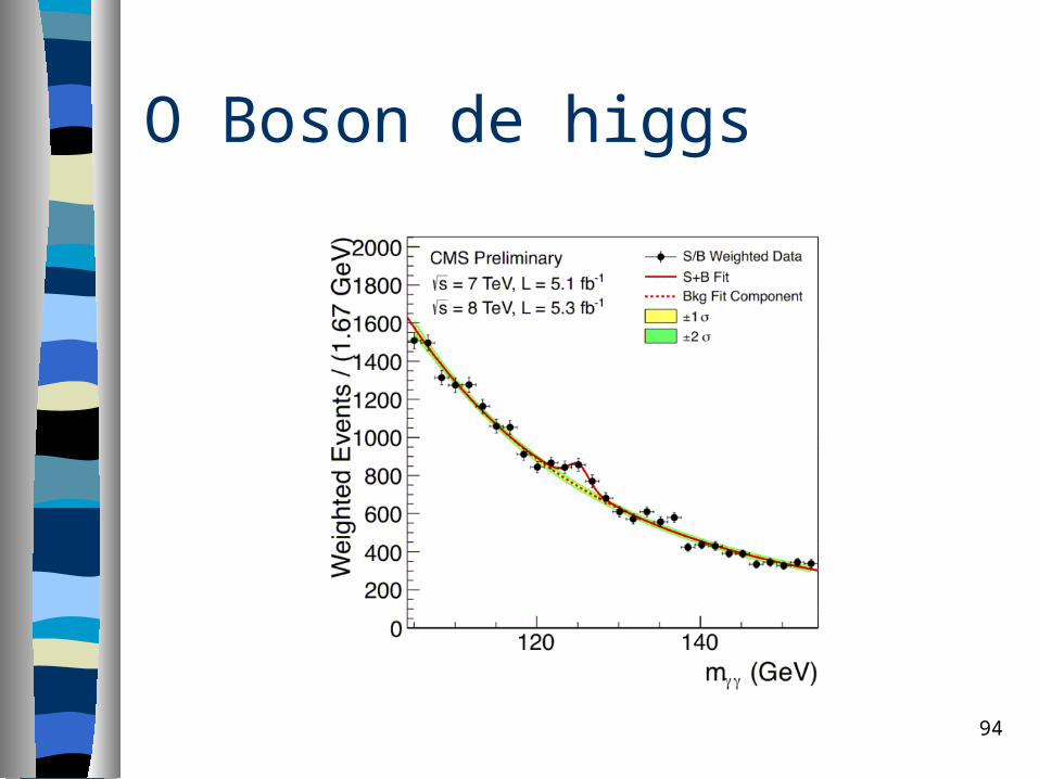
O Boson de higgs

94

Próxima Aula

PCA LDA + MLDA

95

Fim

96

97