Embed Size (px)
Citation preview
Signal Integrity and High-Speed InterconnectsJanuary-May 2006
Dr. J. E. Rayas Sánchezhttp://iteso.mx/~erayas [email protected]
1
Transmission Line Theory(Part 3)
Dr. José Ernesto Rayas Sánchez
2Dr. J.E. Rayas Sánchez
Outline
Input impedance in lossless transmission lines (TL)
Special cases of lossless terminated TL
Insertion loss
Transmission coefficient
Smith Chart interpretation
Basic Smith Chart applications
Signal Integrity and High-Speed InterconnectsJanuary-May 2006
Dr. J. E. Rayas Sánchezhttp://iteso.mx/~erayas [email protected]
3Dr. J.E. Rayas Sánchez
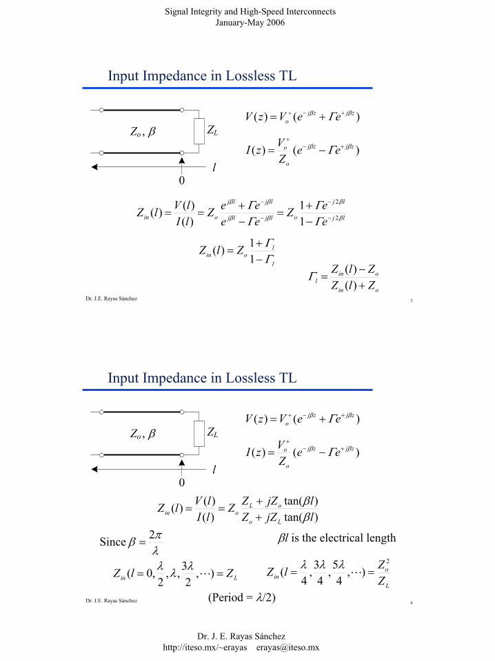
Input Impedance in Lossless TL
Zo , β
0l
ZL
)()( zjzjo eeVzV ββ Γ +−+ +=
)()( zjzj
o
o eeZVzI ββ Γ +−
+
−=
lj
lj
oljlj
ljlj
oin eeZ
eeeeZ
lIlVlZ β
β
ββ
ββ
ΓΓ
ΓΓ
2
2
11
)()()( −
−
−
−
−+=
−+==
l
loin ZlZ
ΓΓ
−+=
11)(
oin
oinl ZlZ
ZlZ+−=
)()(Γ
4Dr. J.E. Rayas Sánchez
Input Impedance in Lossless TL
)tan()tan(
)()()(
ljZZljZZZ
lIlVlZ
Lo
oLoin β
β++==
Lin ZlZ == ),2
3,,2
,0( Lλλλ
λπβ 2 Since =
L
oin Z
ZlZ2
),4
5,4
3,4
( == Lλλλ
(Period = λ/2)
Zo , β
0l
ZL
)()( zjzjo eeVzV ββ Γ +−+ +=
)()( zjzj
o
o eeZVzI ββ Γ +−
+
−=
βl is the electrical length
Signal Integrity and High-Speed InterconnectsJanuary-May 2006
Dr. J. E. Rayas Sánchezhttp://iteso.mx/~erayas [email protected]
5Dr. J.E. Rayas Sánchez
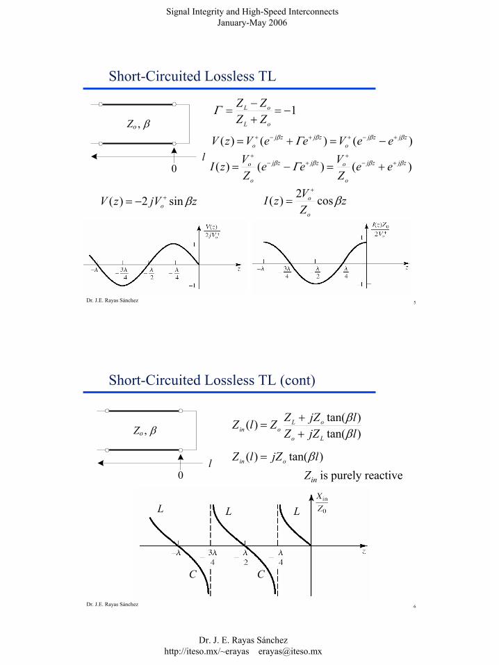
Short-Circuited Lossless TL
Zo , β
0l
)()()( zjzjo
zjzjo eeVeeVzV ββββ Γ +−++−+ −=+=
)()()( zjzj
o
ozjzj
o
o eeZVee
ZVzI ββββ Γ +−
++−
+
+=−=
1−=+−=
oL
oL
ZZZZΓ
zjVzV o βsin2)( +−= zZVzI
o
o βcos2)(+
=
6Dr. J.E. Rayas Sánchez
Short-Circuited Lossless TL (cont)
)tan()tan()(
ljZZljZZZlZ
Lo
oLoin β
β++=Zo , β
0l )tan()( ljZlZ oin β=
Zin is purely reactive
C
LLL
C
Signal Integrity and High-Speed InterconnectsJanuary-May 2006
Dr. J. E. Rayas Sánchezhttp://iteso.mx/~erayas [email protected]
7Dr. J.E. Rayas Sánchez
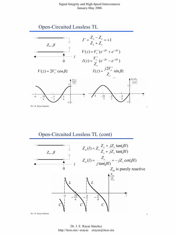
Open-Circuited Lossless TL
Zo , β
0l
1+=+−=
oL
oL
ZZZZΓ
)()( zjzjo eeVzV ββ +−+ +=
)()( zjzj
o
o eeZVzI ββ +−
+
−=
zVzV o βcos2)( += zZVjzIo
o βsin2)(+
=
8Dr. J.E. Rayas Sánchez
Open-Circuited Lossless TL (cont)
)tan()tan()(
ljZZljZZZlZ
Lo
oLoin β
β++=
)cot()tan(
)( ljZlj
ZlZ oo
in ββ
−==
Zin is purely reactive
Zo , β
0l
LL
C CC
Signal Integrity and High-Speed InterconnectsJanuary-May 2006
Dr. J. E. Rayas Sánchezhttp://iteso.mx/~erayas [email protected]
9Dr. J.E. Rayas Sánchez
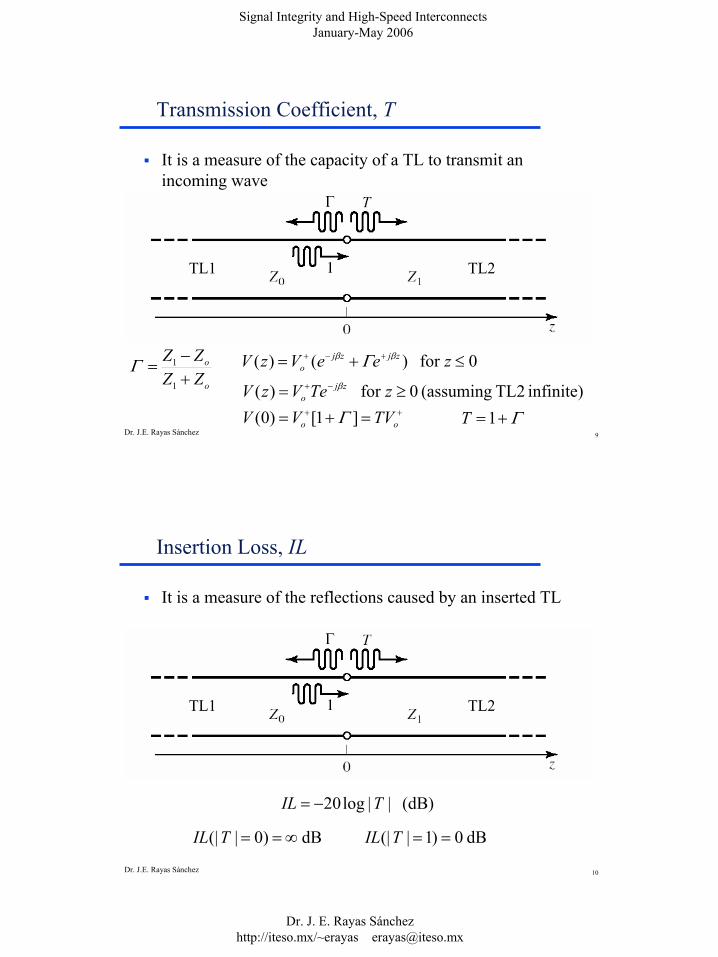
Transmission Coefficient, T
It is a measure of the capacity of a TL to transmit an incoming wave
0for )()( ≤+= +−+ zeeVzV zjzjo
ββ Γo
o
ZZZZ
+−=
1
1Γinfinite) TL2 (assuming 0for )( ≥= −+ zTeVzV zj
oβ
TL2TL1
++ =+= oo TVVV ]1[)0( Γ Γ+=1T
10Dr. J.E. Rayas Sánchez
Insertion Loss, IL
It is a measure of the reflections caused by an inserted TL
TL2TL1
(dB) ||log20 TIL −=
dB)0|(| ∞==TIL dB0)1|(| ==TIL
Signal Integrity and High-Speed InterconnectsJanuary-May 2006
Dr. J. E. Rayas Sánchezhttp://iteso.mx/~erayas [email protected]
11Dr. J.E. Rayas Sánchez
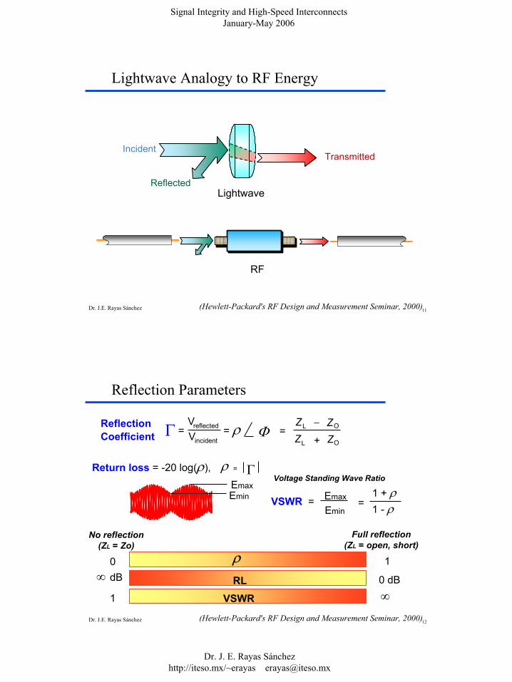
Lightwave Analogy to RF Energy
RF
Incident
Reflected
Transmitted
Lightwave
(Hewlett-Packard's RF Design and Measurement Seminar, 2000)
12Dr. J.E. Rayas Sánchez
Reflection Parameters
∞ dB
No reflection(ZL = Zo)
ρRL
VSWR
0 1
Full reflection(ZL = open, short)
0 dB
1 ∞
=ZL − ZO
ZL + OZReflectionCoefficient =
Vreflected
Vincident= ρ ΦΓ
=ρ ΓReturn loss = -20 log(ρ),
VSWR = Emax
Emin=
1 + ρ1 - ρ
Voltage Standing Wave RatioEmaxEmin
(Hewlett-Packard's RF Design and Measurement Seminar, 2000)
Signal Integrity and High-Speed InterconnectsJanuary-May 2006
Dr. J. E. Rayas Sánchezhttp://iteso.mx/~erayas [email protected]
13Dr. J.E. Rayas Sánchez
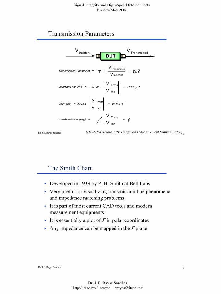
Transmission Parameters
(Hewlett-Packard's RF Design and Measurement Seminar, 2000)
V TransmittedV Incident
Transmission Coefficient = Τ =VTransmitted
VIncident= τ∠φ
DUT
Gain (dB) = 20 Log V Trans
V Inc = 20 log τ
Insertion Loss (dB) = - 20 Log V Trans
V Inc = - 20 log τ
Insertion Phase (deg) = V Trans
V Inc = φ
14Dr. J.E. Rayas Sánchez
The Smith Chart
Developed in 1939 by P. H. Smith at Bell LabsVery useful for visualizing transmission line phenomena and impedance matching problemsIt is part of most current CAD tools and modern measurement equipmentsIt is essentially a plot of Γ in polar coordinatesAny impedance can be mapped in the Γ plane
Signal Integrity and High-Speed InterconnectsJanuary-May 2006
Dr. J. E. Rayas Sánchezhttp://iteso.mx/~erayas [email protected]
15Dr. J.E. Rayas Sánchez
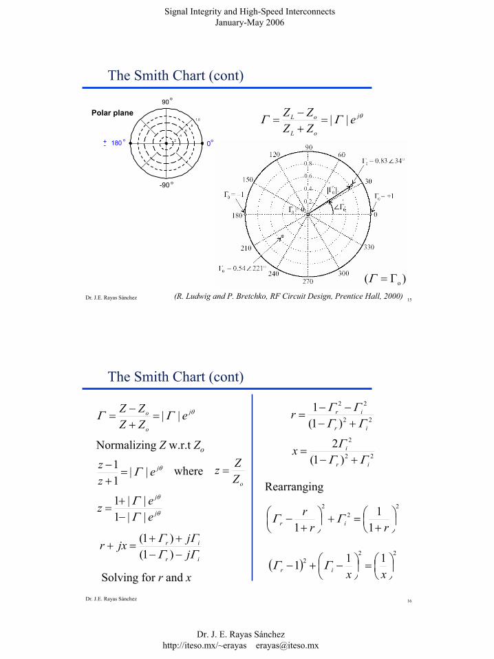
The Smith Chart (cont)
-90 o
0o180 o+-.2
.4.6
.8
1.0
90 o
Polar plane θΓΓ j
oL
oL eZZZZ ||=
+−=
(R. Ludwig and P. Bretchko, RF Circuit Design, Prentice Hall, 2000)
)Γ( o=Γ
16Dr. J.E. Rayas Sánchez
The Smith Chart (cont)
θΓΓ j
o
o eZZZZ ||=
+−=
Normalizing Z w.r.t Zo
θΓ jezz ||
11 =
+− where
oZZz =
θ
θ
ΓΓ
j
j
eez
||1||1
−+=
ir
ir
jjjxrΓΓΓΓ
−−++=+
)1()1(
22
22
)1(1
ir
irrΓΓ
ΓΓ+−
−−=
22
2
)1(2
ir
ixΓΓ
Γ+−
=
22
2
11
1
+=+
+−
rrr
ir ΓΓ
( )22
2 111
=
−+−
xxir ΓΓSolving for r and x
Rearranging
Signal Integrity and High-Speed InterconnectsJanuary-May 2006
Dr. J. E. Rayas Sánchezhttp://iteso.mx/~erayas [email protected]
17Dr. J.E. Rayas Sánchez
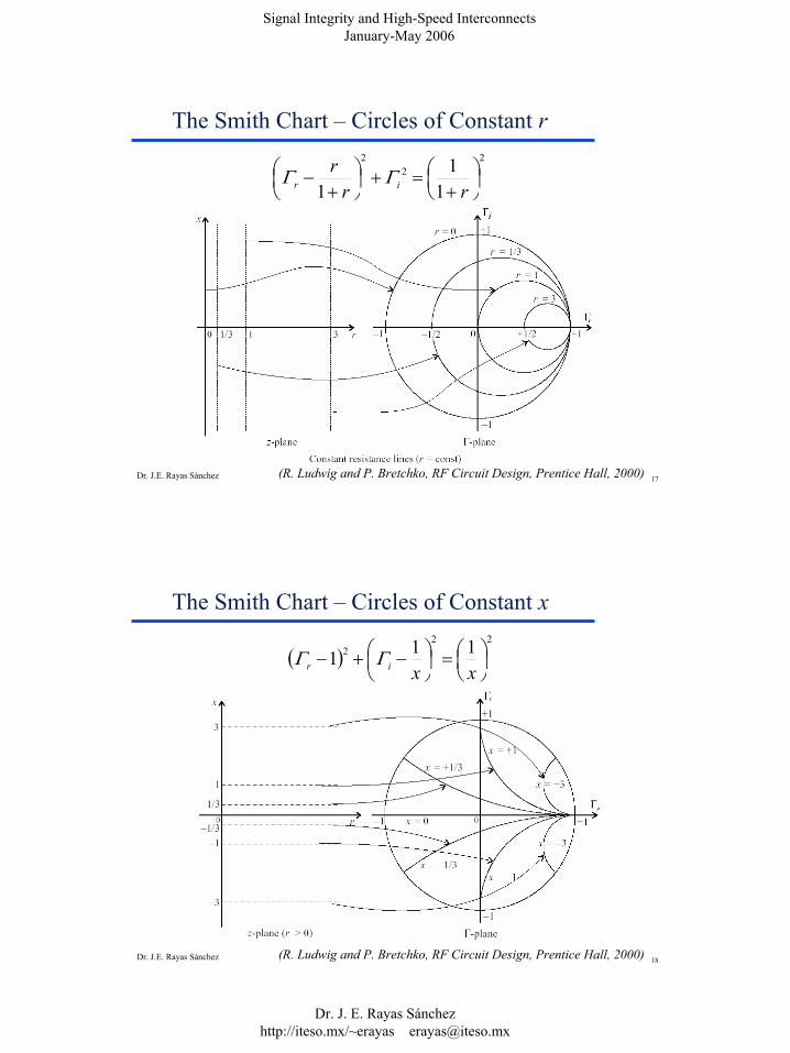
The Smith Chart – Circles of Constant r
(R. Ludwig and P. Bretchko, RF Circuit Design, Prentice Hall, 2000)
22
2
11
1
+=+
+−
rrr
ir ΓΓ
18Dr. J.E. Rayas Sánchez
The Smith Chart – Circles of Constant x
(R. Ludwig and P. Bretchko, RF Circuit Design, Prentice Hall, 2000)
( )22
2 111
=
−+−
xxir ΓΓ
Signal Integrity and High-Speed InterconnectsJanuary-May 2006
Dr. J. E. Rayas Sánchezhttp://iteso.mx/~erayas [email protected]
19Dr. J.E. Rayas Sánchez
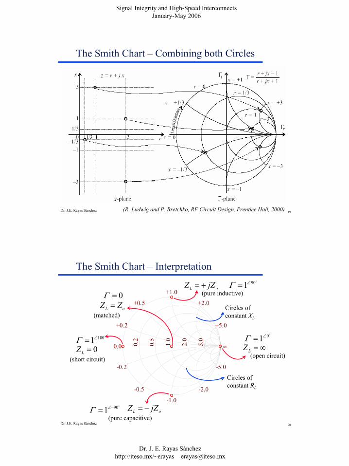
The Smith Chart – Combining both Circles
(R. Ludwig and P. Bretchko, RF Circuit Design, Prentice Hall, 2000)
20Dr. J.E. Rayas Sánchez
The Smith Chart – Interpretation
0=LZ
0.2
0.5
1.0
2.0
5.0
+0.2
-0.2
+0.5
-0.5
+1.0
-1.0
+2.0
-2.0
+5.0
-5.0
0.0 ∞ ∞=LZ
oL ZZ =
oL jZZ −=
oL jZZ +=
(open circuit)(short circuit)
(pure inductive)
(pure capacitive)
(matched)Circles of constant XL
Circles of constant RL
0=Γ
o1801∠=Γo01∠=Γ
o901∠=Γ
o901 −∠=Γ
Signal Integrity and High-Speed InterconnectsJanuary-May 2006
Dr. J. E. Rayas Sánchezhttp://iteso.mx/~erayas [email protected]
21Dr. J.E. Rayas Sánchez
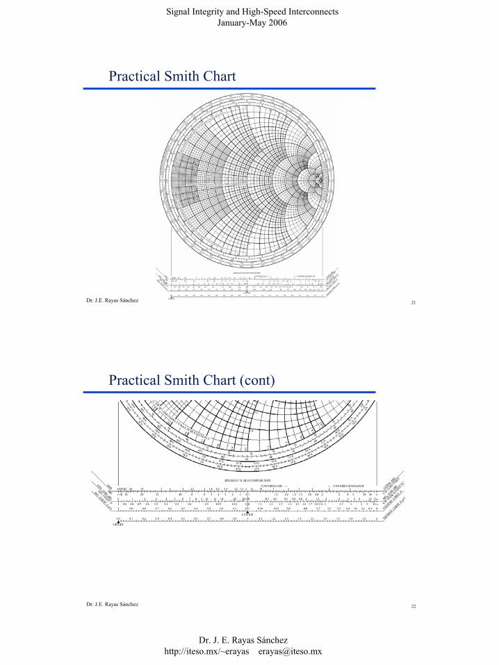
Practical Smith Chart
22Dr. J.E. Rayas Sánchez
Practical Smith Chart (cont)
Signal Integrity and High-Speed InterconnectsJanuary-May 2006
Dr. J. E. Rayas Sánchezhttp://iteso.mx/~erayas [email protected]
23Dr. J.E. Rayas Sánchez
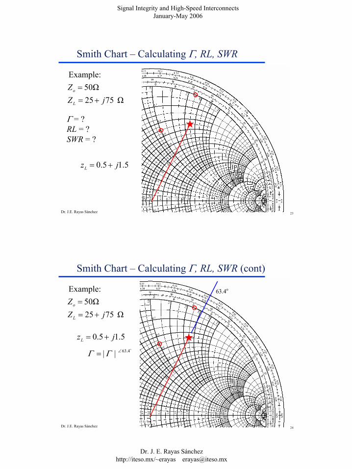
Smith Chart – Calculating Γ, RL, SWR
Example:Ω50=oZ
Ω 7525 jZL +=
5.15.0 jzL +=
Γ = ?RL = ?SWR = ?
24Dr. J.E. Rayas Sánchez
Smith Chart – Calculating Γ, RL, SWR (cont)
Example:Ω50=oZ
Ω 7525 jZL +=
63.4o
5.15.0 jzL +=o4.63|| ∠= ΓΓ

Signal Integrity and High-Speed InterconnectsJanuary-May 2006
Dr. J. E. Rayas Sánchezhttp://iteso.mx/~erayas [email protected]
25Dr. J.E. Rayas Sánchez
Smith Chart – Calculating Γ, RL, SWR (cont)
Example:Ω50=oZ
Ω 7525 jZL +=
5.15.0 jzL +=o4.63|| ∠= ΓΓ
26Dr. J.E. Rayas Sánchez
Smith Chart – Calculating Γ, RL, SWR (cont)
Example:Ω50=oZ
Ω 7525 jZL +=
5.15.0 jzL +=o4.6375.0 ∠≈Γ
0.75
7
2.57≈SWR
dB 5.2≈RL
Signal Integrity and High-Speed InterconnectsJanuary-May 2006
Dr. J. E. Rayas Sánchezhttp://iteso.mx/~erayas [email protected]
27Dr. J.E. Rayas Sánchez
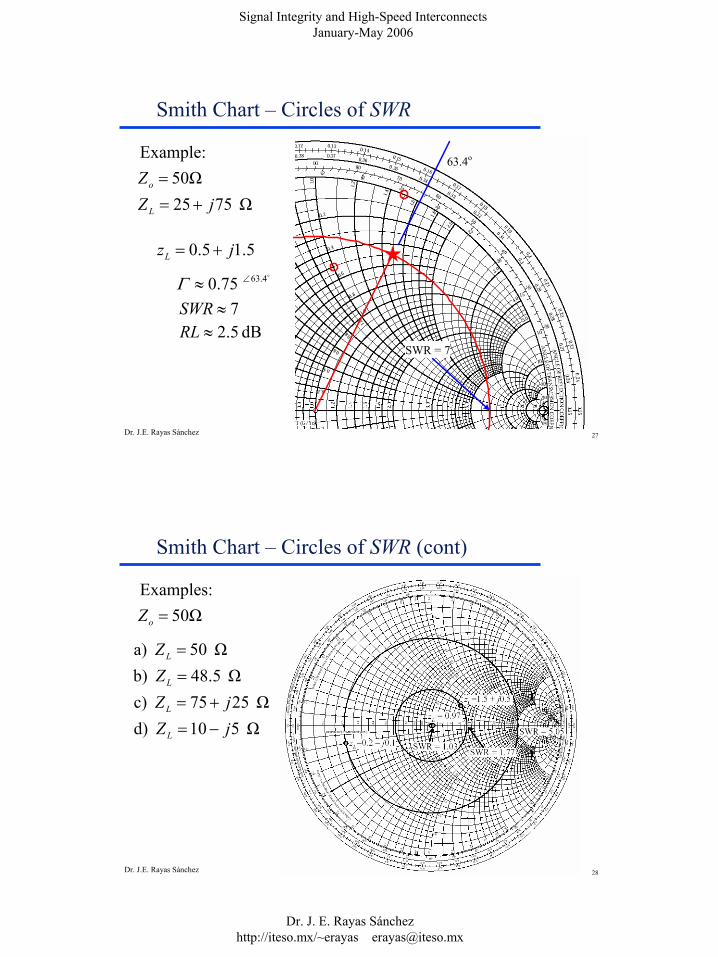
Smith Chart – Circles of SWR
Example:Ω50=oZ
Ω 7525 jZL +=
5.15.0 jzL +=o4.6375.0 ∠≈Γ
7≈SWRdB 5.2≈RL
63.4o
SWR = 7
28Dr. J.E. Rayas Sánchez
Smith Chart – Circles of SWR (cont)
Examples:Ω50=oZ
Ω 2575 c) jZL +=
Ω 50 a) =LZΩ 5.48 b) =LZ
Ω 510 d) jZL −=
Signal Integrity and High-Speed InterconnectsJanuary-May 2006
Dr. J. E. Rayas Sánchezhttp://iteso.mx/~erayas [email protected]
29Dr. J.E. Rayas Sánchez
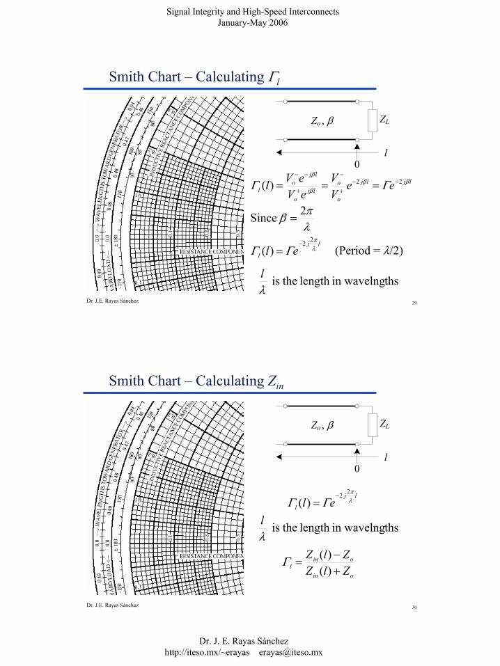
Smith Chart – Calculating Γl
ljlj
o
olj
o
ljo
l eeVV
eVeVl ββ
β
β
ΓΓ 22)( −−+
−
+
−−
===
Zo , β
0l
ZL
λπβ 2 Since =
(Period = λ/2)lj
l el λπ
ΓΓ22
)(−
=
thsin wavelnglength theis λl
30Dr. J.E. Rayas Sánchez
Smith Chart – Calculating Zin
Zo , β
0l
ZL
oin
oinl ZlZ
ZlZ+−=
)()(Γ
lj
l el λπ
ΓΓ22
)(−
=
thsin wavelnglength theis λl
Signal Integrity and High-Speed InterconnectsJanuary-May 2006
Dr. J. E. Rayas Sánchezhttp://iteso.mx/~erayas [email protected]
31Dr. J.E. Rayas Sánchez
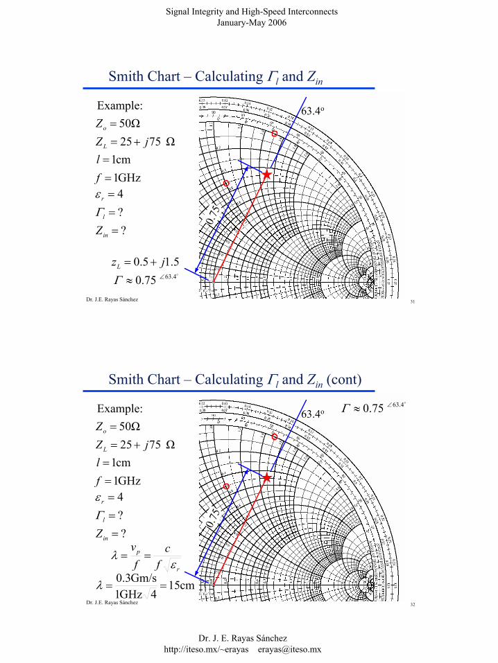
Smith Chart – Calculating Γl and Zin
Example:Ω50=oZ
Ω 7525 jZL +=cm1=lGHz1=f4=rε?=lΓ?=inZ
5.15.0 jzL +=o4.6375.0 ∠≈Γ
63.4o
0.75
32Dr. J.E. Rayas Sánchez
63.4o
0.75
Smith Chart – Calculating Γl and Zin (cont)
Example:Ω50=oZ
Ω 7525 jZL +=cm1=lGHz1=f4=rε?=lΓ?=inZ
o4.6375.0 ∠≈Γ
r
p
fc
fv
ελ ==
cm154GHz1
Gm/s3.0 ==λ
Signal Integrity and High-Speed InterconnectsJanuary-May 2006
Dr. J. E. Rayas Sánchezhttp://iteso.mx/~erayas [email protected]
33Dr. J.E. Rayas Sánchez
63.4o
0.75
Smith Chart – Calculating Γl and Zin (cont)
Example:Ω50=oZ
Ω 7525 jZL +=cm1=lGHz1=f4=rε?=lΓ?=inZ
o4.6375.0 ∠≈Γ
067.0cm15
cm1 ==λl
229.0067.0162.0 =+
34Dr. J.E. Rayas Sánchez
63.4o
0.75
15o
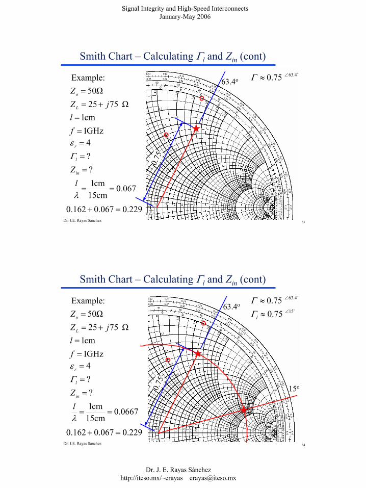
Smith Chart – Calculating Γl and Zin (cont)
Example:Ω50=oZ
Ω 7525 jZL +=cm1=lGHz1=f4=rε?=lΓ?=inZ
o4.6375.0 ∠≈Γ
0667.0cm15
cm1 ==λl
229.0067.0162.0 =+
o1575.0 ∠≈lΓ
Signal Integrity and High-Speed InterconnectsJanuary-May 2006
Dr. J. E. Rayas Sánchezhttp://iteso.mx/~erayas [email protected]
35Dr. J.E. Rayas Sánchez
63.4o
0.75
15o
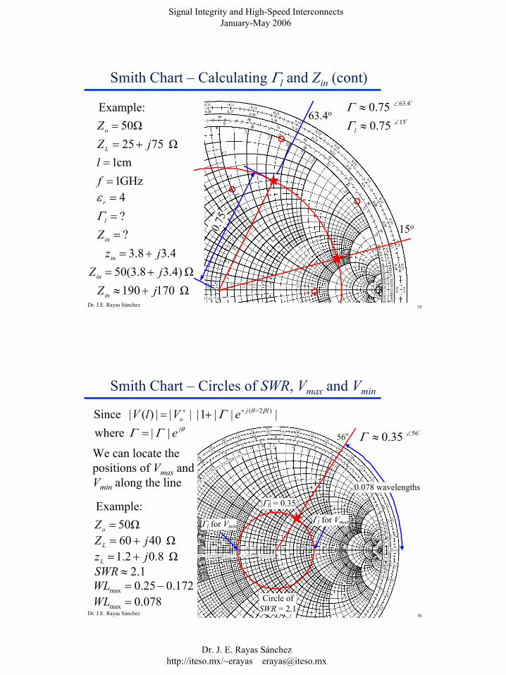
Smith Chart – Calculating Γl and Zin (cont)
Example:Ω50=oZ
Ω 7525 jZL +=cm1=lGHz1=f4=rε?=lΓ?=inZ
o4.6375.0 ∠≈Γo1575.0 ∠≈lΓ
4.38.3 jzin +=Ω )4.38.3(50 jZin +=Ω 170190 jZin +≈
36Dr. J.E. Rayas Sánchez
Smith Chart – Circles of SWR, Vmax and Vmin
Example:Ω50=oZ
Ω 4060 jZL +=Ω 8.02.1 jzL +=
1.2≈SWR
θΓΓ je|| where =|||1||||)(| Since )2( lj
o eVlV βθΓ −++ +=
We can locate the positions of Vmax and Vmin along the line
56o
Circle of SWR = 2.1
Γl for VmaxΓl for Vmin
|Γl| = 0.35
0.078 wavelengths
172.025.0max −=WL078.0max =WL
o5635.0 ∠≈Γ