Embed Size (px)
Citation preview
DOI 10.1393/ncb/i2009-10742-6
Basic topics: Fundamental Physics
IL NUOVO CIMENTO Vol. 124 B, N. 1 Gennaio 2009
True explanation of operation of homopolar engine
A. Radovic
Spasovdanksa 13a, 11030 Beograd, Serbia
(ricevuto il 4 Settembre 2008; revisionato il 17 Marzo 2009; approvato il 18 Marzo 2009; pub-blicato online il 6 Maggio 2009)
Summary. — Operation of Faraday’s homopolar engine had crucial aftermaths tocontemporary science. Most of misunderstandings of the machine’s operation causedwrong acceptance of N hypothesis instead of M one. Although there were plenty ofauthors suspecting that physical fields are moveable, this fact is finally duly provenby the experiment depicted in the text. There are also analyzed classical stringtheoretical concept with fields’ equations and the induction formula.
PACS 84.50.+d – Electric motors.PACS 03.50.De – Classical electromagnetism, Maxwell equations.PACS 07.55.Db – Generation of magnetic fields; magnets.PACS 13.40.-f – Electromagnetic processes and properties.
1. – Introduction
At the beginning of the 19th century there was great arguing between advocates ofM hypothesis and of N hypothesis. M hypothesis denotes a concept of physical realityin which the physical fields have their own velocities and these velocities mainly matchthe velocities of the fields’ sources. N hypothesis is a concept of physical reality in whichthe physical fields do not have their own velocities and therefore physical sources, i.e.poles just change the magnitude of the eternally existing fields without affecting theirown velocities at all. This standpoint is based on the conviction that the concept ofphysical fields represents rather a mathematical generalization of force’s action than areal thing. Therefore mathematical imagination or fiction cannot have a plausible velocitythat reflects something real.
The N hypothesis won the M hypothesis after the famous Faraday’s experiment withthe homopolar generator was performed and that allegedly proved that N hypothesis isthe only valid one. Furthermore, this generator was the first electric machine ever builtand consequently it was a milestone for all subsequent physical theories. The aftermathof this experiment to the following development of theoretical electromagnetism wastremendous: Maxwell equations had to have total time derivatives instead of partial onesto prevent propagation of the time derivative to the coordinate which would transform thecoordinate into the velocity and this is not possible within N hypothesis simply because
c© Societa Italiana di Fisica 13
14 A. RADOVIC
BB
ωM
ωd
R
V
ωM
D
B1
M
SM
B2
V
E1
E2
SD
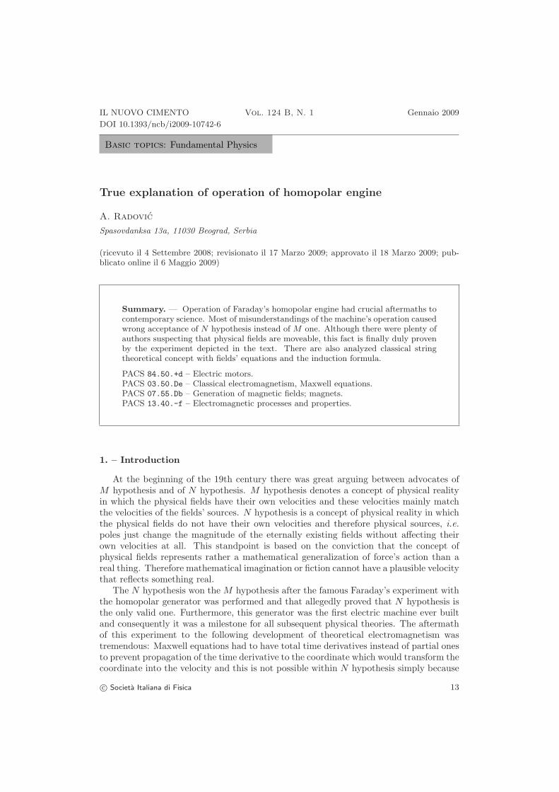
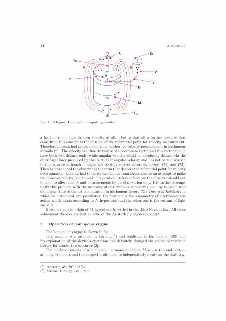
Fig. 1. – Original Faraday’s homopolar generator.
a field does not have its own velocity at all. Due to that all a further obstacle thatcame from this concept is the absence of the referential point for velocity measurement.Therefore Lorentz had problems to define anchor for velocity measurement in his famousformula (2). The velocity is a time derivative of a coordinate vector and this vector shouldhave both well-defined ends, while angular velocity could be absolutely defined via thecentrifugal force produced by this particular angular velocity and has not been discussedin this treatise although it might not be duly correct according to eqs. (71) and (72).Then he introduced the observer as the term that denotes the referential point for velocitydetermination. Lorentz had to derive his famous transformations as an attempt to makethe observer relative, i.e. to make his position irrelevant because the observer should notbe able to affect reality and measurements by his observation only. His further attemptto fix this problem with the necessity of observer’s existence was done by Einstein whodid a true state-of-the-art computation in his famous theory The Theory of Relativity inwhich he introduced two postulates: the first one is the asymmetry of electromagneticaction which exists according to N hypothesis and the other one is the costant of lightspeed [1].
It seems that the origin of M hypothesis is settled in the third Newton law. All thesesubsequent theories are just an echo of the Aristotle(1) physical concept.
2. – Operation of homopolar engine
The homopolar engine is shown in fig. 1.This machine was invented by Faraday(2) and published in his book in 1831 and
his explanation of the device’s operation had definitely changed the course of mankindhistory for almost two centuries [2].
The machine consists of a homopolar permanent magnet M whose top and bottomare magnetic poles and this magnet is also able to independently rotate on the shaft SM .
(1) Aristotle, 384 BC-322 BC.(2) Michael Faraday, 1791-1867.
TRUE EXPLANATION OF OPERATION OF HOMOPOLAR ENGINE 15
Above the magnet there is a non-magnetic conductive disk D also able to freely rotateon shaft SD with respect to laboratory. A voltmeter V is attached via external partsof the electric circuit E1 and E2 to brushes B1 and B2, respectively; brush B2 createscontact to shaft SD and another brush B1 creates contact to the brim of the disk D too.
The main apparently amazing characteristic of this machine that astonished Faradayand his coevals was the fact that the angular velocity of the permanent magnet Mmeasured on any way has no influence on the generated voltage output at all—only theangular velocity(3) of the disk D affects the induction measured on the voltmeter V whichperfectly matches the following theoretical formula (�ω⊥�r and �ω⊥ �B and �r⊥ �B, detailedderivation in [3]):
(1) V =∫ r
0
(�ω × �r ) × �B · d�r =ωdisc · B · r2
2.
This is based on the following equation:
(2) �E = �v × �B.
In the text below it will be shown that the proper form of the above equation should be
(3) �E1 = �v1,2 × �B1.
Faraday was claiming that the field is non-motional (i.e. that N hypothesis is valid)and he finally proved the concept experimentally with the above machine now known asFaraday’s Homopolar Generator and then M hypothesis was abandoned. This proof wasbased on the fact that the rotation of the homopolar magnet does not have any influenceon the induction itself and the consequential conclusion is that the magnetic field does nothave its own velocity. Aftermath of the conclusion was the necessity of an involvementof observer’s concept into classical electromagnetic theory, simply because velocity ineq. (83) could not be defined in regards to something that does not have its own velocityat all. Lorentz(4) tried to resolve this problem with the attempt of relativization ofthe observer’s concept known as Lorentz transformations. A fully evolved theory of theobserver’s relativization was finally developed later by Einstein(5).
But, official Faraday’s explanation seems to be incorrect, which is pretty obvious fromthe rearrangement of the above machinery (fully described in [3]).
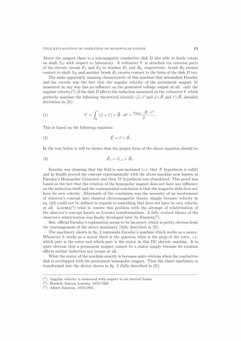
The machinery shown in fig. 2 represents Faraday’s machine which works as a motor.Whenever it works as a motor there is the question what is the prop of the rotor, i.e.which part is the rotor and which part is the stator in this DC electric machine. It isquite obvious that a permanent magnet cannot be a stator simply because its rotationaffects neither induction nor torque at all.
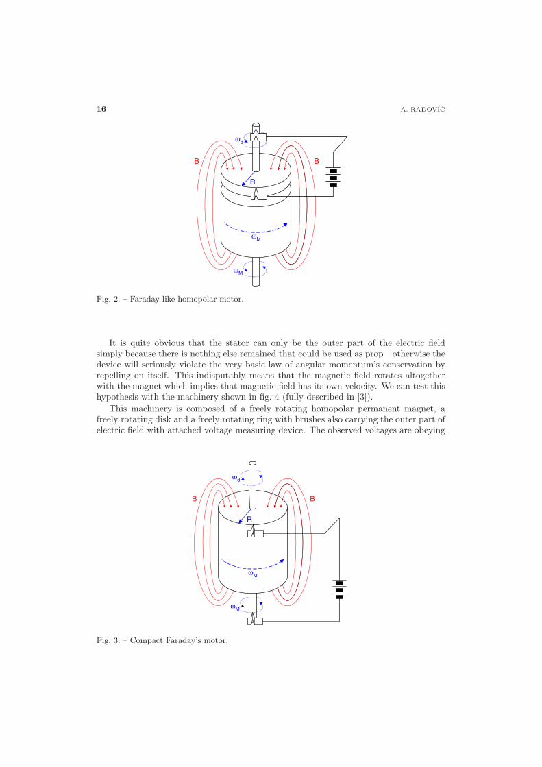
What the stator of the machine exactly is becomes quite obvious when the conductivedisk is overlapped with the permanent homopolar magnet. Then the above machinery istransformed into the device shown in fig. 3 (fully described in [3]).
(3) Angular velocity is measured with respect to an inertial frame.(4) Hendrik Antoon Lorentz, 1853-1928.(5) Albert Einstein, 1879-1955.
16 A. RADOVIC
BB
ωM
ωd
R
ωM
Fig. 2. – Faraday-like homopolar motor.
It is quite obvious that the stator can only be the outer part of the electric fieldsimply because there is nothing else remained that could be used as prop—otherwise thedevice will seriously violate the very basic law of angular momentum’s conservation byrepelling on itself. This indisputably means that the magnetic field rotates altogetherwith the magnet which implies that magnetic field has its own velocity. We can test thishypothesis with the machinery shown in fig. 4 (fully described in [3]).
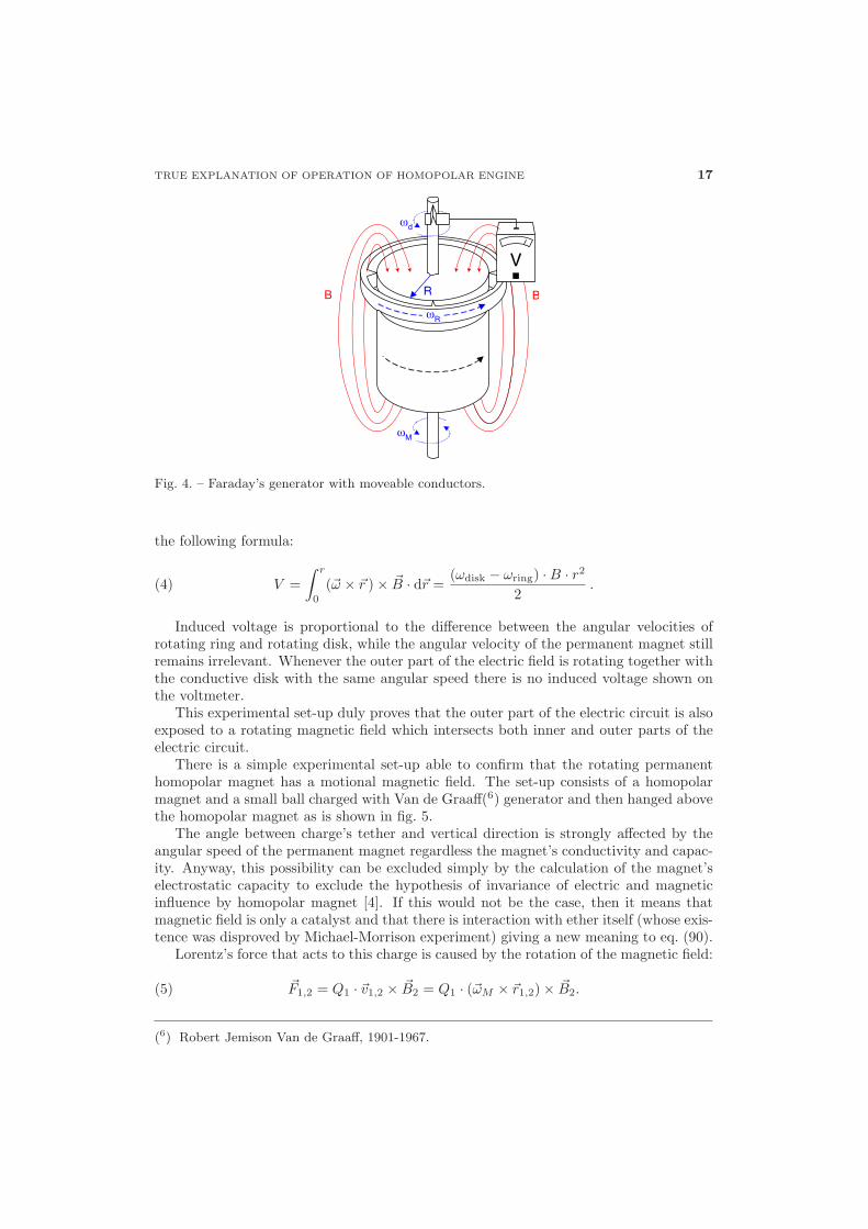
This machinery is composed of a freely rotating homopolar permanent magnet, afreely rotating disk and a freely rotating ring with brushes also carrying the outer part ofelectric field with attached voltage measuring device. The observed voltages are obeying
BB
ωM
ωd
R
ωM
Fig. 3. – Compact Faraday’s motor.
TRUE EXPLANATION OF OPERATION OF HOMOPOLAR ENGINE 17
BB
ωM
ωd
R
V
ωR
Fig. 4. – Faraday’s generator with moveable conductors.
the following formula:
(4) V =∫ r
0
(�ω × �r ) × �B · d�r =(ωdisk − ωring) · B · r2
2.
Induced voltage is proportional to the difference between the angular velocities ofrotating ring and rotating disk, while the angular velocity of the permanent magnet stillremains irrelevant. Whenever the outer part of the electric field is rotating together withthe conductive disk with the same angular speed there is no induced voltage shown onthe voltmeter.
This experimental set-up duly proves that the outer part of the electric circuit is alsoexposed to a rotating magnetic field which intersects both inner and outer parts of theelectric circuit.
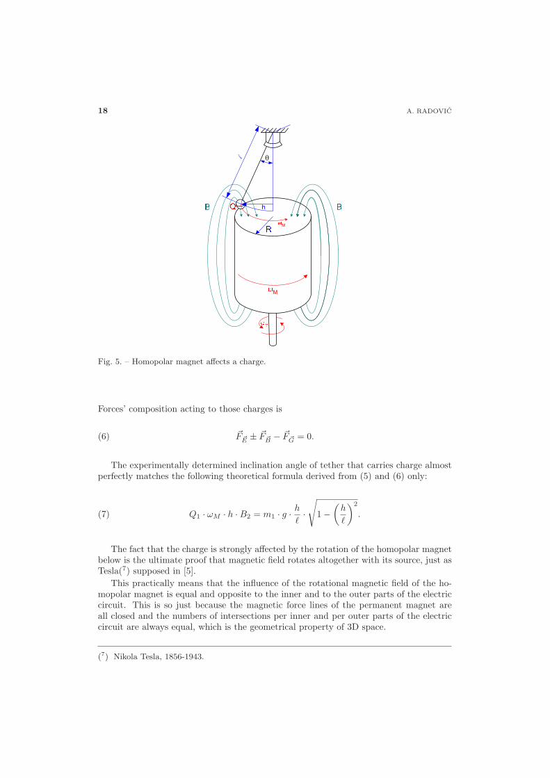
There is a simple experimental set-up able to confirm that the rotating permanenthomopolar magnet has a motional magnetic field. The set-up consists of a homopolarmagnet and a small ball charged with Van de Graaff(6) generator and then hanged abovethe homopolar magnet as is shown in fig. 5.
The angle between charge’s tether and vertical direction is strongly affected by theangular speed of the permanent magnet regardless the magnet’s conductivity and capac-ity. Anyway, this possibility can be excluded simply by the calculation of the magnet’selectrostatic capacity to exclude the hypothesis of invariance of electric and magneticinfluence by homopolar magnet [4]. If this would not be the case, then it means thatmagnetic field is only a catalyst and that there is interaction with ether itself (whose exis-tence was disproved by Michael-Morrison experiment) giving a new meaning to eq. (90).
Lorentz’s force that acts to this charge is caused by the rotation of the magnetic field:
(5) �F1,2 = Q1 · �v1,2 × �B2 = Q1 · (�ωM × �r1,2) × �B2.
(6) Robert Jemison Van de Graaff, 1901-1967.
18 A. RADOVIC
l
θ
h
M
M
Fig. 5. – Homopolar magnet affects a charge.
Forces’ composition acting to those charges is
(6) �F�E ± �F �B − �F�G = 0.
The experimentally determined inclination angle of tether that carries charge almostperfectly matches the following theoretical formula derived from (5) and (6) only:
(7) Q1 · ωM · h · B2 = m1 · g · h
�·
√1 −
(h
�
)2
.
The fact that the charge is strongly affected by the rotation of the homopolar magnetbelow is the ultimate proof that magnetic field rotates altogether with its source, just asTesla(7) supposed in [5].
This practically means that the influence of the rotational magnetic field of the ho-mopolar magnet is equal and opposite to the inner and to the outer parts of the electriccircuit. This is so just because the magnetic force lines of the permanent magnet areall closed and the numbers of intersections per inner and per outer parts of the electriccircuit are always equal, which is the geometrical property of 3D space.
(7) Nikola Tesla, 1856-1943.
TRUE EXPLANATION OF OPERATION OF HOMOPOLAR ENGINE 19
1 1
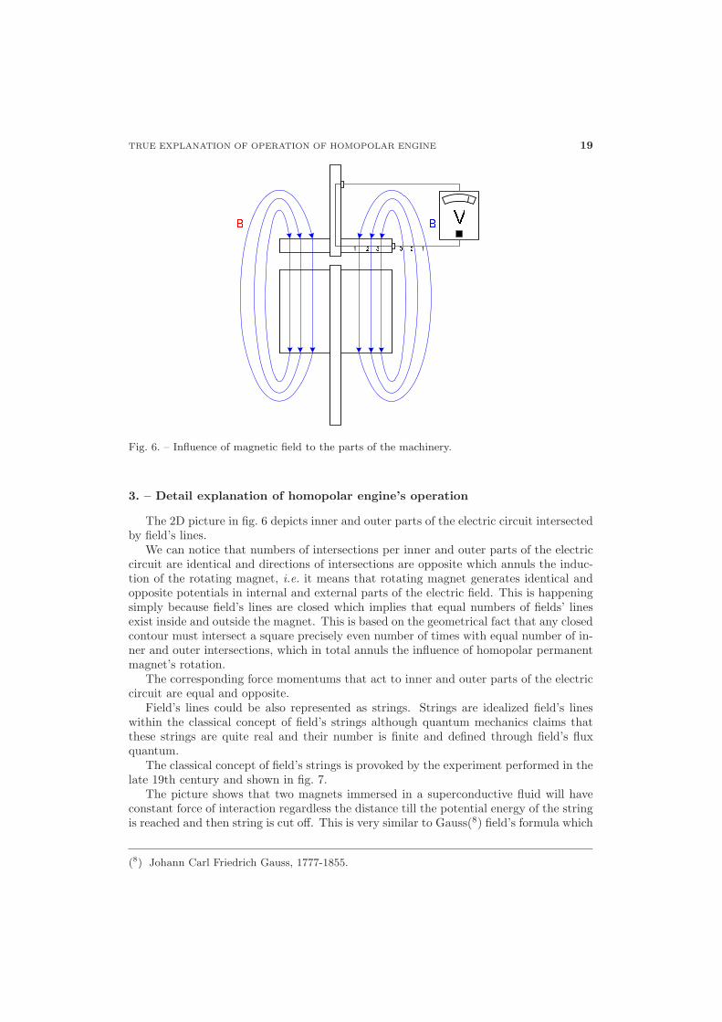
Fig. 6. – Influence of magnetic field to the parts of the machinery.
3. – Detail explanation of homopolar engine’s operation
The 2D picture in fig. 6 depicts inner and outer parts of the electric circuit intersectedby field’s lines.
We can notice that numbers of intersections per inner and outer parts of the electriccircuit are identical and directions of intersections are opposite which annuls the induc-tion of the rotating magnet, i.e. it means that rotating magnet generates identical andopposite potentials in internal and external parts of the electric field. This is happeningsimply because field’s lines are closed which implies that equal numbers of fields’ linesexist inside and outside the magnet. This is based on the geometrical fact that any closedcontour must intersect a square precisely even number of times with equal number of in-ner and outer intersections, which in total annuls the influence of homopolar permanentmagnet’s rotation.
The corresponding force momentums that act to inner and outer parts of the electriccircuit are equal and opposite.
Field’s lines could be also represented as strings. Strings are idealized field’s lineswithin the classical concept of field’s strings although quantum mechanics claims thatthese strings are quite real and their number is finite and defined through field’s fluxquantum.
The classical concept of field’s strings is provoked by the experiment performed in thelate 19th century and shown in fig. 7.
The picture shows that two magnets immersed in a superconductive fluid will haveconstant force of interaction regardless the distance till the potential energy of the stringis reached and then string is cut off. This is very similar to Gauss(8) field’s formula which
(8) Johann Carl Friedrich Gauss, 1777-1855.

20 A. RADOVIC
Fig. 7. – String in E1 space.
is just the continuum equation of field’s lines:
(8) ρ = ε · �∇ �E.
In classical field’s string theory we should define the potential as the number of stringsthat intersects a wire per time:
(9) U =dN �B
dt.
The magnetic field is defined as a concentration of strings penetrating the surface:
(10) �B =dN �B
d�S.
And also
(11) �E =dN�E
d�S=
1ε· dQ
d�S.
Directly from Gauss law we have
(12) N�E =�S
�E · d�S =Q
ε.
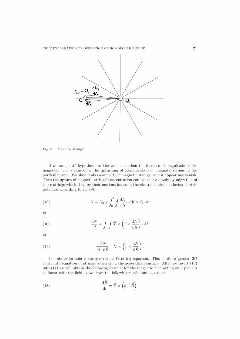
String’s force between poles is then defined as
(13) �F1,2 = Q1 ·dN2
d�S1
.
Also
(14) �F2,1 = Q2 ·dN1
d�S2
= −�F1,2.
This concept is depicted in fig. 8.
TRUE EXPLANATION OF OPERATION OF HOMOPOLAR ENGINE 21
1,22
211
11
Fig. 8. – Force by strings.
If we accept M hypothesis as the valid one, then the increase of magnitude of themagnetic field is caused by the upturning of concentration of magnetic strings in theparticular area. We should also assume that magnetic strings cannot appear nor vanish.Then the upturn of magnetic strings’ concentration can be achieved only by migration ofthose strings which then by their motions intersect the electric contour inducing electricpotential according to eq. (9):
(15) N = N0 +∫ t
0
∮t
dN
d�S· (d�� × �v) · dt
⇒
(16)dN
dt=
∫S
∫�∇×
(�v × dN
d�S
)· d�S
⇒
(17)d2N
dt · d�S= �∇×
(�v × dN
d�S
).
The above formula is the general field’s string equation. This is also a general 2Dcontinuity equation of strings penetrating the generalized surface. After we insert (10)into (17) we will obtain the following formula for the magnetic field acting on a plane ncollinear with the field, so we have the following continuum equation:
(18)d �B
dt= �∇×
(�v × �B
).
22 A. RADOVIC
where �B denotes the magnetic field and �v denotes the velocity of magnetic field’s lines’migration. We can generalize the above equation to all persistent physical fields orig-inated in their non-decaying poles with uniform strings’ distribution including gravityfield too, so within M hypothesis the next equation of gravitational field is valid:
(19)d�G
dt= �∇×
(�v × �G
).
Classical string theory’s formula of electric field is
(20)d �E
dt= �∇×
(�v × �E
).
After (10) is inserted into (9) we have
(21) U =ddt
�S
�B · d�S =dΦdt
,
where U is the electric potential, B is the magnetic field, S is the element of the area, tis the time and Φ is the flux of the magnetic field.
The above equation is a precise derivation of Gaussian induction’s formula. It isdirectly derived by string idealization within M hypothesis of motional magnetic field.
After Stokes(9) mathematical transformation is applied to the above equation andpotential is replaced with its definition, it is derived:
(22)�S
�∇× �E · d�S =ddt
�S
�B · d�S.
The above equation can be differentiated on surface and then we obtain the firstMaxwell(10) equation:
(23) �∇× �E =d �B
dt.
It should be noticed that there are total time derivatives in the Maxwell equationswithin M hypothesis instead of partial ones.
We have just seen that the equation which corresponds to the first Maxwell equationis actually just a formula for migration of magnetic lines, but the second Maxwell-likeequation cannot be derived with such elegance.
This second Maxwell-like equation could be derived directly from both empiricBiot(11)-Savart(12) law and eq. (20):
(24) d �B1 = − μ
4 · π · I1 · d��1 × r1,2
�r 21,2
,
(9) George Gabriel Stokes, 1819-1903.(10) James C. Maxwell, 1831-1879.(11) Jean-Baptiste Biot, 1774-1862.(12) Felix Savart, 1791-1841.
TRUE EXPLANATION OF OPERATION OF HOMOPOLAR ENGINE 23
where I is the electric current, r1,2 is the distance between the current element andmeasuring position, d� is the infinitesimal current path and B1 is the magnetic field onthe test position.
The above equation can be modified in the following way:
(25) d �B1 = − μ
4 · π ·dqdt · d�r1,2 × r1,2
�r 21,2
=�v1,2
c2× 1
4 · π · ε · dq · r1,2
�r 21,2
= −�v1,2
c2× d �E.
After integration we have
(26) �B = −�v × �E
c2=
�E × �v
c2.
After Curl is applied on the above equation and with the help of (20) we have
(27) �∇× �B =�∇×
(�v × �E
)c2
= − 1c2
· d �E
dt
and
(28) c2 · �∇× �B = −d �E
dt.
We have eqs. (23) and (28) that correspond to Maxwell ones. While there are totaltime derivatives in both (23) and (28) there is no need for missing DC term with currentdensity which describes the appearance of the magnetic field near conductors with directconstant current only. This term was artificially added in official Maxwell equation justto keep its ability to handle appearance of constant magnetic field near DC conductors.
After eq. (28) is slightly rearranged and multiplied with imaginary unit i, we have
(29) i · c · �∇× �B = − ic· d �E
dt,
where i is the imaginary unit, c is the speed of light, E is the electric field and B is themagnetic field.
After (23) is added to the above equation we have
(30) �∇× �E + i · c · �∇× �B =d �B
dt− i
c· d �E
dt.
This equation is then rearranged into the following form:
(31) i · c · �∇×(
�E + i · c · �B)
=ddt
(�E + c · i · �B
).
Let us denote the complex electromagnetic field with K:
(32) �K = �E + i · c · �B.
24 A. RADOVIC
Thus we have the following recursive relation of complex electromagnetic field �K:
(33) i · c · �∇× �Kj+1 =d �Kj
dt.
Equation (33) is a single equation containing only complex electromagnetic field �K andthat equation corresponds to Maxwell ones.
We also have the following non-recursive general formula of field’s migration:
(34)d �K
dt= �∇×
(�v × �K
).
Directly from (33) and (34) we have a quite interesting relation:
(35) �Kn+1 = −i ·(
�v
c
)× �Kn
⇒
(36) �Kn+2 =(
1 +�v2
c2
)· �Kn −
(�v · �Kn
)· �v
c2.
The formula for energy density (i.e. pressure) of the complex electromagnetic field is
(37) P �K = ε ·�K · conj( �K)
2.
The corresponding Poynting(13) vector is
(38) �P �K = ε ·�K × conj( �K)
2.
Proof of (37) is based on official fields’ energy density equations that are
(39) P�E =ε · �E2
2
and
(40) P �B =�B2
2 · μ .
Classical strings theory yields a slightly different result for energy density in the field.From (11) we have
(41) dQ = ε ·(
�E · d�S)
.
(13) John Poynting, 1852-1914.
TRUE EXPLANATION OF OPERATION OF HOMOPOLAR ENGINE 25
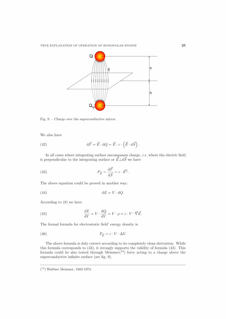
Fig. 9. – Charge over the superconductive mirror.
We also have
(42) d�F = �E · dQ = �E · ε ·(
�E · d�S)
.
In all cases where integrating surface encompasses charge, i.e. where the electric fieldis perpendicular to the integrating surface or �E⊥d�S we have
(43) P�E =d�F
d�S= ε · �E2.
The above equation could be proved in another way:
(44) dE = V · dQ.
According to (8) we have
(45)dE
dV= V · dQ
dV= V · ρ = ε · V · �∇ �E.
The formal formula for electrostatic field’ energy density is
(46) P�E = ε · V · ΔV.
The above formula is duly correct according to its completely clean derivation. Whilethis formula corresponds to (43), it strongly supports the validity of formula (43). Thisformula could be also tested through Meissner(14) force acting to a charge above thesuperconductive infinite surface (see fig. 9).
(14) Walther Meissner, 1882-1974.
26 A. RADOVIC
According to image theory we have that the force acting between real charge andghost charge is
(47) FQ,QG=
14 · π · ε · Q2
(2 · h)2=
Q2
16 · π · h2.
Miessner force that corresponds to Archimedes(15) force in liquids is
(48) �FQ,QG=
�S
P�E · d�S =�S
k · ε · �E2 · d�S.
The coefficient k should be determined by equalization of eqs. (47) and (48):
(49) k · ε · Q2
(4 · π · ε)2 ·∫ ∞
−∞
∫ ∞
−∞
dx · dy
(h2 + x2 + y2)2=
Q2
16 · π · h2
⇒
(50) k = 1.
By these three independent proofs we could accept that official energy density for-mula (39) should not be halved at all.
However, this halving does not affect the following formulas because it is canceling inthose equations. Formula (39) clearly shows that energy source of the field is the poleitself and that without the pole there is no energy in the field.
Total energy density according to the official approach is
(51) P = P�E + P �B =ε · �E2
2+
�B2
2 · μ
⇒
(52)2 · P
ε= �E2 + (c · �B)2.
Equation (52) clearly shows that both terms �E and c · �B have equal units makingformula (33) quite plausible. Force acting to a charge in a complex field is
(53) �F = Q · �K.
The proof of the above equation is clear:
(54) �F = Q · �E + Q · �v × �B = Q ·�K + conj( �K)
2+ Q · �v ×
�K − conj( �K)2 · i · c
(15) Archimedes of Syracuse, 287 BC-212 BC.
TRUE EXPLANATION OF OPERATION OF HOMOPOLAR ENGINE 27
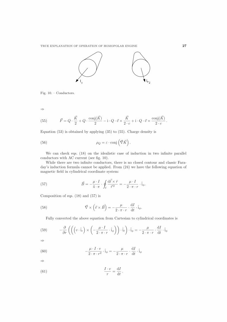
Fig. 10. – Conductors.
⇒
(55) �F = Q ·�K
2+ Q · conj( �K)
2− i · Q · �v ×
�K
2 · c + i · Q · �v × conj( �K)2 · c .
Equation (53) is obtained by applying (35) to (55). Charge density is
(56) ρQ = ε · conj(
�∇ �K)
.
We can check eqs. (18) on the idealistic case of induction in two infinite parallelconductors with AC current (see fig. 10).
While there are two infinite conductors, there is no closed contour and classic Fara-day’s induction formula cannot be applied. From (24) we have the following equation ofmagnetic field in cylindrical coordinate system:
(57) �B = −μ · I4 · π ·
∮�
d�� × r
�r 2= − μ · I
2 · π · r · iφ.
Composition of eqs. (18) and (57) is
(58) �∇×(�v × �B
)= − μ
2 · π · r · dI
dt· iφ.
Fully converted the above equation from Cartesian to cylindrical coordinates is
(59) − ∂
∂r
(((v · ir
)×
(− μ · I
2 · π · r · iφ))
· i�)· iφ = − μ
2 · π · r · dI
dt· iφ
⇒
(60) − μ · I · v2 · π · r2
· iφ = − μ
2 · π · r · dI
dt· iφ
⇒
(61)I · vr
=dI
dt.
28 A. RADOVIC
We can find migration speed of magnetic field of a straight infinite conductor withAC current now:
(62) �v =r
I· dI
dt· ir.
It is interesting to notice that the migration velocity can be superluminal too.We can insert the above formula into (2) and then we have
(63) �E = �v× �B =(
r
I· dI
dt
)·(− μ · I
2 · π · r
)·(ir × iφ
)=
μ
2 · π · dI
dt· i� =
μ
2 · π · dQ
dt·a · i�.
Induced electric field is collinear with the conductor just as is the case with transformerand the polarity matches the transformer’s reality. Force acting to a charge nearby theinfinite conductor is
(64) �F = Q ·(�v �B − �vQ
)× �B =
μ · Q2 · π · i� ·
⎛⎝dI
dt−
I ·(�vQ · ir
)r
⎞⎠ .
where �v �B is the velocity of the magnetic field itself and �vQ is the velocity of the chargewith respect to the conductor. The above formula has excellent matching with realexperiment and shows that the maximal speed of the charge is limited by the speed ofthe magnetic field itself.
If the conductors are long enough to be approximated with infinite parallel conductors,then we have that the potential is proportional to the length of the conductors:
(65) V = �E · �� =μ · �2 · π · dI
dt.
This unique ability to yield correct induction’s formula based on magnetic field’smigration (62) is a clear proof of the correctness of the whole concept.
The above notification can be generalized in the following way. After time derivation,eq. (26) becomes
(66)d �B
dt=
�E × �a
c2.
According to appropriate Maxwell-like equation we have
(67) �∇× �Eind =�E × �a
c2.
There is also a general vector identity:
(68) �E × �a = �∇× (V · �a) − V · �∇× �a.
Therefore we have
(69) �∇× �E =�∇× (V · �a)
c2− V · �∇× �a
c2.
TRUE EXPLANATION OF OPERATION OF HOMOPOLAR ENGINE 29
The additional electric field induced by acceleration added to a particle in the electricpotential V is
(70) �Eind ≈ V · �ac2
.
The inertial phenomenon of electron becomes
(71) �Finertial = Q1 · �Eind =Q1 · V2 · �a1,2
c2=
μ · Q1 · Q2 · �r1,2
4 · π · |�r1,2|.
For mass we have
(72) �Find =γ
c2· m1 · m2 · �a1,2
|�r| = m1 · �a1,2 ·Vgrav2
c2.
The above formula defines the connection between induced electric field in secondaryconductor and acceleration of charges in primary conductor. According to this formulainertia of charged particle is caused by the external potential that pervades it.
Another very interesting formula can be obtained directly from (20):
(73)d �E
dt= �∇×
(Q
4 · π · ε · ⇀r
2 · �v × r
),
⇒
(74)d �E
dt= �∇×
(Q
4 · π · ε · |⇀r |· �ω
),
⇒
(75)d �E
dt= �∇× (V · �ω).
With the help of (28) we have
(76) �B ≈ −V · �ωc2
.
The above formula could be proved by independent line of equations. The formulafor mutual angular velocity between two moving points is
(77) �ω1,2 =�r1,2 × �r1,2
�r 21,2
=�r1,2 × r1,2
|�r1,2|=
�v1,2 × r1,2
|�r1,2|.
According to (26) and (77) we have
(78) �B1 =�v1,2 × �E1,2
c2=
�v1,2
c2× Q1 · r1,2
4 · π · ε · �r 21,2
= −V · �ω1,2
c2.

30 A. RADOVIC
Fig. 11. – Magnetic domains.
Total induced electric field according to eqs. (2), (70) and (76) is
(79) �Eind = V · �a + �v × �ω
c2.
The above formula shows that the magnetic field of a rotating punctual charge isproportional to the scalar product of rotation and the electric potential of the particle.This clearly shows that the magnetic field is a torsion electric potential.
It is interesting to notice that
(80)d2 |�r1,2|
dt2= (�a1,2 + �v1,2 × �ω1,2) · r1,2.
The term in brackets denotes total acceleration, which clearly proves that electromag-netic induction is indisputably connected to the acceleration.
Magnetic domains created by elementary particles’ rotation can be represented in thepicture shown in fig. 11.
Formula (79) is very interesting because it proves that mutual acceleration in electricfield cases induced an electric field able to make the operation of the electric transformerthrough AC induction possible, which is pure M hypothesis’ phenomenon.
Almost all basic equations from the classical electromagnetic theory can be preciselyderived by introduction of M hypothesis of moveable physical fields. Ability of all theseelectromagnetic correct derivations is the proof that exposed string’s idealization of arbi-trary physical field is physically plausible and mathematically correct. This idealizationis the only available concept able to duly explain the operation of Faraday’s homopolarengine. It is interesting that Mach(16) principle could be proven within M hypothesistoo because distribution of physical fields’ string is not necessarily uniform.
(16) Ernst Mach, 1838-1916.
TRUE EXPLANATION OF OPERATION OF HOMOPOLAR ENGINE 31
( )12
k
!12k2
kƒ−
π
−⋅=
( )
12 2.2 2.4 2.6 2.8 3
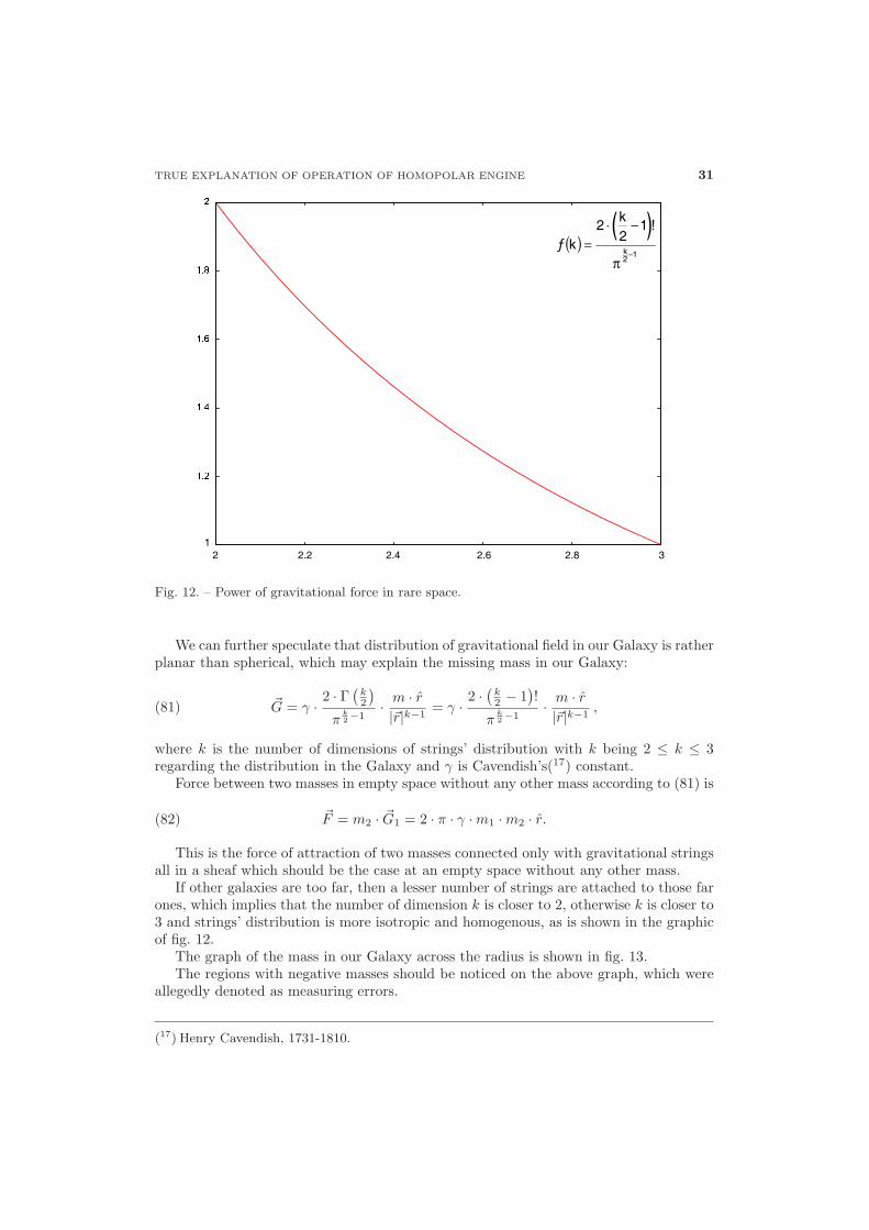
Fig. 12. – Power of gravitational force in rare space.
We can further speculate that distribution of gravitational field in our Galaxy is ratherplanar than spherical, which may explain the missing mass in our Galaxy:
(81) �G = γ ·2 · Γ
(k2
)π
k2−1
· m · r|�r|k−1
= γ ·2 ·
(k2 − 1
)!
πk2−1
· m · r|�r|k−1
,
where k is the number of dimensions of strings’ distribution with k being 2 ≤ k ≤ 3regarding the distribution in the Galaxy and γ is Cavendish’s(17) constant.
Force between two masses in empty space without any other mass according to (81) is
(82) �F = m2 · �G1 = 2 · π · γ · m1 · m2 · r.
This is the force of attraction of two masses connected only with gravitational stringsall in a sheaf which should be the case at an empty space without any other mass.
If other galaxies are too far, then a lesser number of strings are attached to those farones, which implies that the number of dimension k is closer to 2, otherwise k is closer to3 and strings’ distribution is more isotropic and homogenous, as is shown in the graphicof fig. 12.
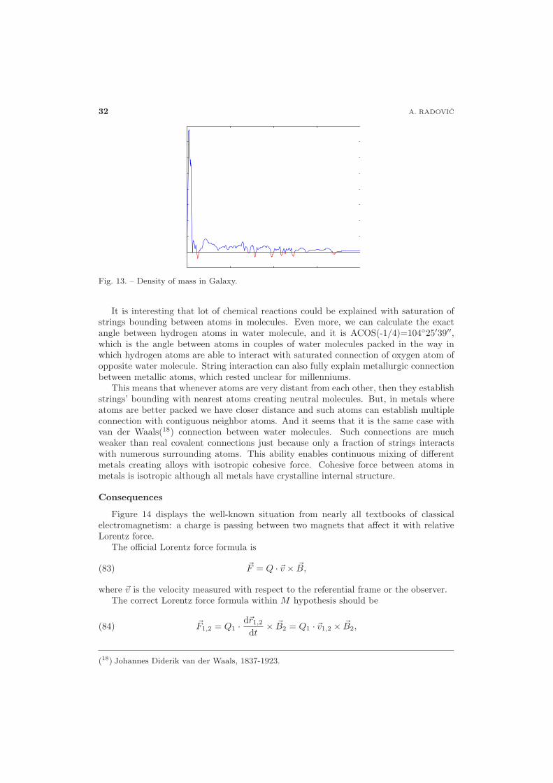
The graph of the mass in our Galaxy across the radius is shown in fig. 13.The regions with negative masses should be noticed on the above graph, which were
allegedly denoted as measuring errors.
(17) Henry Cavendish, 1731-1810.
32 A. RADOVIC
Fig. 13. – Density of mass in Galaxy.
It is interesting that lot of chemical reactions could be explained with saturation ofstrings bounding between atoms in molecules. Even more, we can calculate the exactangle between hydrogen atoms in water molecule, and it is ACOS(-1/4)=104◦25′39′′,which is the angle between atoms in couples of water molecules packed in the way inwhich hydrogen atoms are able to interact with saturated connection of oxygen atom ofopposite water molecule. String interaction can also fully explain metallurgic connectionbetween metallic atoms, which rested unclear for millenniums.
This means that whenever atoms are very distant from each other, then they establishstrings’ bounding with nearest atoms creating neutral molecules. But, in metals whereatoms are better packed we have closer distance and such atoms can establish multipleconnection with contiguous neighbor atoms. And it seems that it is the same case withvan der Waals(18) connection between water molecules. Such connections are muchweaker than real covalent connections just because only a fraction of strings interactswith numerous surrounding atoms. This ability enables continuous mixing of differentmetals creating alloys with isotropic cohesive force. Cohesive force between atoms inmetals is isotropic although all metals have crystalline internal structure.
Consequences
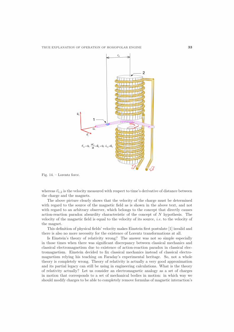
Figure 14 displays the well-known situation from nearly all textbooks of classicalelectromagnetism: a charge is passing between two magnets that affect it with relativeLorentz force.
The official Lorentz force formula is
(83) �F = Q · �v × �B,
where �v is the velocity measured with respect to the referential frame or the observer.The correct Lorentz force formula within M hypothesis should be
(84) �F1,2 = Q1 ·d�r1,2
dt× �B2 = Q1 · �v1,2 × �B2,
(18) Johannes Diderik van der Waals, 1837-1923.
TRUE EXPLANATION OF OPERATION OF HOMOPOLAR ENGINE 33
22,1122,1
12,1 BvQBdtrd
QF ×⋅=×⋅=
2,1r
2B
1E
1Q
1
2
→
→
→
→→
→ → →
Fig. 14. – Lorentz force.
whereas �v1,2 is the velocity measured with respect to time’s derivative of distance betweenthe charge and the magnets.
The above picture clearly shows that the velocity of the charge must be determinedwith regard to the source of the magnetic field as is shown in the above text, and notwith regard to an arbitrary observer, which belongs to the concept that directly causesaction-reaction paradox absurdity characteristic of the concept of N hypothesis. Thevelocity of the magnetic field is equal to the velocity of its source, i.e. to the velocity ofthe magnet.
This definition of physical fields’ velocity makes Einstein first postulate [1] invalid andthere is also no more necessity for the existence of Lorentz transformations at all.
Is Einstein’s theory of relativity wrong? The answer was not so simple especiallyin those times when there was significant discrepancy between classical mechanics andclassical electromagnetism due to existence of action-reaction paradox in classical elec-tromagnetism. Einstein decided to fix classical mechanics instead of classical electro-magnetism relying his teaching on Faraday’s experimental heritage. So, not a wholetheory is completely wrong. Theory of relativity is actually a very good approximationand its partial legacy can still be using in engineering calculations. What is the theoryof relativity actually? Let us consider an electromagnetic analogy as a set of chargesin motion that corresponds to a set of mechanical bodies in motion: in which way weshould modify charges to be able to completely remove formulas of magnetic interaction’s
34 A. RADOVIC
and to keep the correct results of forces in those mutual interactions like in the previouscase when magnetic interaction still has been calculated? It can be easily shown thatcharges should be modified in the same way as Einstein did it with mass. Could it be acompletely correct transformation? No, it is impossible to cancel magnetic field and tocalculate interaction with respect to a unique observer instead of calculation of the sumof mutual electrostatic and magnetic interactions between particular participants in theinteraction and still to keep results identical. Charge as scalar does not carry enoughinformation in Coulomb’s(19) force formula and thus for better accuracy charge shouldbe represented as tensor. The same improvement in mass description can be done withNewton(20) gravity force formula too, which then resembles the major concept of specialtheory of relativity. So, the theories of relativity are able to yield pretty correct resultsfor interaction of two mutual participants because observer’s velocity is usually very closeto velocity of the one participant. Finally, a special theory of relativity is able to yield acorrect formula of Cherenkov’s radiation and also to predict circumstances suitable formagnetons existence [6] implying that both of these theories require not so serious lifting.
Is there any experimental evidence proving that the theory of relativity is not com-pletely true? Yes, there are plenty of evidences: stellar aberration, ability to be mea-sured absolute velocity with respect to background radiation with Doppler’s(21) effect,Boomerang Project [7], etc. Simple proof against the theory of relativity is: if the onewho is moving faster has slower passing of time, then there is the question who is the bossthat should judge who is moving slower and who faster, which contradicts Galilean(22)relativity of the velocity. Obviously, there must be an arbitrary observer to judge thatotherwise Einstein’s theory does not have sense at all. Another solid proof against theabsolute consistency of the general theory of relativity is the discrepancy between thecenter of inertial and the center of gravitational masses of the same body. The centerof gravitational mass is not generally identical to the center of the inertial mass of anarbitrary shaped body, as shown by the following formula:
(85)√
m ·�
V�r
|�r|3 · ρm(�r ) · dV∣∣∣� V�r
|�r|3 · ρm(�r ) · dV∣∣∣3/2
�=�
V�r · ρm(�r ) · dV
m.
This inequality vigorously challenges Einstein’s identifications of inertial and gravi-tational masses in his general theory of relativity. Whereas the center of gravitationalmass is defined by
(86) �r�G =√
m ·�
V�r
|�r|3 · ρm(�r ) · dV∣∣∣� V�r
|�r|3 · ρm(�r ) · dV∣∣∣3/2
.
But the center of inertial mass is defined by
(87) �rm =
�V�r · ρm(�r ) · dV
m.
(19) Charles-Augustin de Coulomb, 1736-1806.(20) Isaac Newton, 1643-1727.(21) Johann Christian Andreas Doppler, 1803-1853.(22) Galileo Galilei, 1564-1642.
TRUE EXPLANATION OF OPERATION OF HOMOPOLAR ENGINE 35
The theory of relativity is also a very well circular theory that seriously violatesGodel(23) theorem. We can argue whether there are circumstances with fuzzy logic inwhich Godel theorem is not correct, but the first postulate still remains a fact whoseincorrectness is duly proven in the above text. Metrology divides all physical variablesonto absolute and relative ones. Time and acceleration belong to absolute variables,but velocity and electric potential belong to relative ones and thus relativity of timecan be related only to acceleration, not to velocity if there is any kind of relativity atall as we just suspect it has to be. So, Einstein’s theory of relativity definitely requiresimprovement. At the moment we should accept Einstein legacy just as an excellent set offormulas for variation of mass on subluminal velocities and nothing more. It is a ratherexcellent interpolation made just as an attempt to fix another preceding also incompletetheory rather than a well-founded physical truth.
4. – Origin of the blunder
It seems that the origin of Faraday’s flaw is settled in the third Newton law which wasrelying on Aristotle concept of physics. This law is commonly known in the followingform:
(88) �F = m · �a,
where �F is a force acting to the body that produces acceleration, m is the mass of thebody, �a is the acceleration of the body caused by the force �F . The official explanation isthat the acceleration �a is measured with regard to the inertial frame which is the synonymfor the rocket’s position in which accelerometer will show no acceleration. Such definitionbelongs to the class of logical errors called “Petitio Principi” or circular definition.
But, a basic definition of acceleration is given as the second time derivative of theradius vector whose ends should be well defined with points 1 and 2, respectively:
(89) �a1,2 =d2�r1,2
dt2.
According to the above formula (88) is going to have a more precise form:
(90) �F1,2 = m1 ·d2�r1,2
dt2.
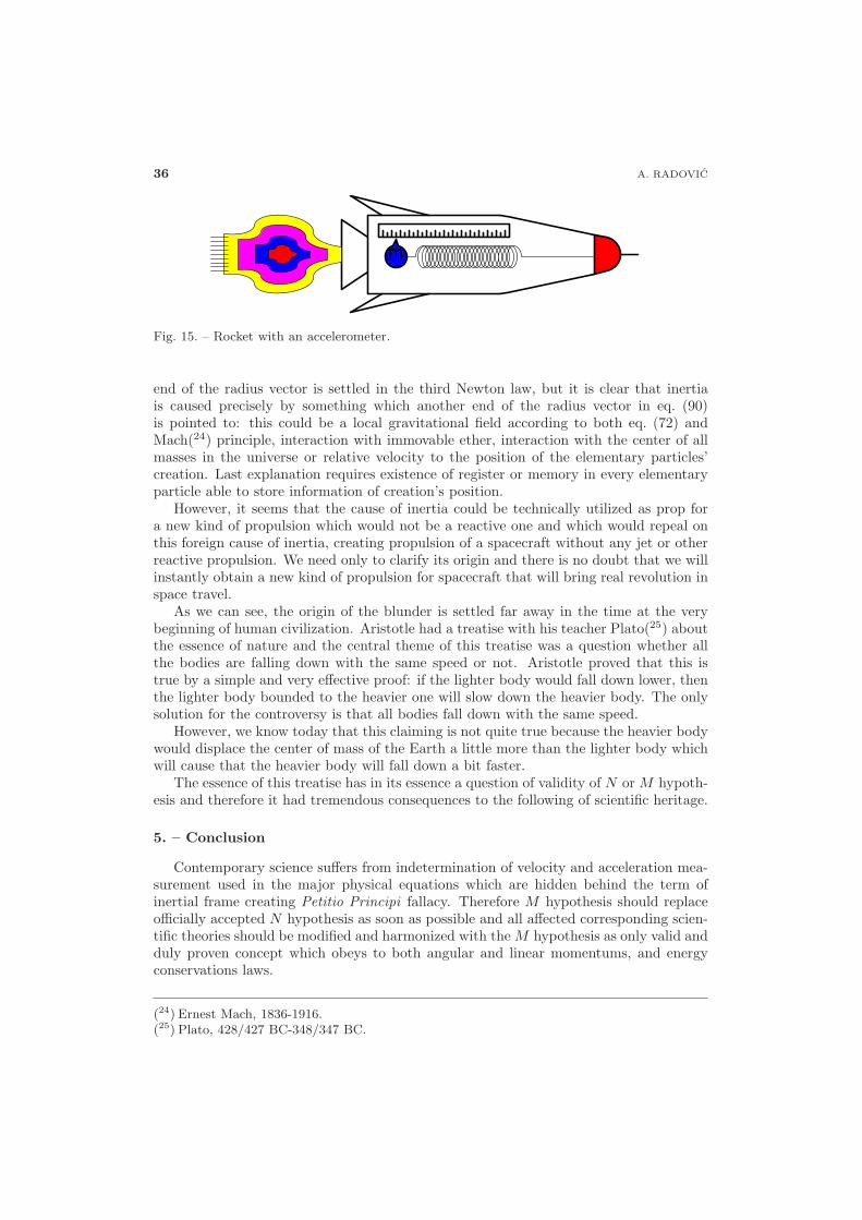
According to the above equation one end of the radius vector is pointed to the mass,while the position of another end of the vector remains undefined. Description of theabove equation’s ambiguity is depicted in the picture shown in fig. 15.
The above picture shows a rocket with an accelerometer: the accelerometer consists ofa small mass attached to a spring. After the rocket’s motor is started this accelerometeris going to measure some acceleration according to compression of the spring and wedo not need to have another referential point available as is necessary in the case ofvelocity’s measurement—furthermore, the accelerometer will remain unconfused even inopen cosmos far away from any cosmic body. So, still there is a question where another
(23) Kurt Godel, 1906-1978.
36 A. RADOVIC
Fig. 15. – Rocket with an accelerometer.
end of the radius vector is settled in the third Newton law, but it is clear that inertiais caused precisely by something which another end of the radius vector in eq. (90)is pointed to: this could be a local gravitational field according to both eq. (72) andMach(24) principle, interaction with immovable ether, interaction with the center of allmasses in the universe or relative velocity to the position of the elementary particles’creation. Last explanation requires existence of register or memory in every elementaryparticle able to store information of creation’s position.
However, it seems that the cause of inertia could be technically utilized as prop fora new kind of propulsion which would not be a reactive one and which would repeal onthis foreign cause of inertia, creating propulsion of a spacecraft without any jet or otherreactive propulsion. We need only to clarify its origin and there is no doubt that we willinstantly obtain a new kind of propulsion for spacecraft that will bring real revolution inspace travel.
As we can see, the origin of the blunder is settled far away in the time at the verybeginning of human civilization. Aristotle had a treatise with his teacher Plato(25) aboutthe essence of nature and the central theme of this treatise was a question whether allthe bodies are falling down with the same speed or not. Aristotle proved that this istrue by a simple and very effective proof: if the lighter body would fall down lower, thenthe lighter body bounded to the heavier one will slow down the heavier body. The onlysolution for the controversy is that all bodies fall down with the same speed.
However, we know today that this claiming is not quite true because the heavier bodywould displace the center of mass of the Earth a little more than the lighter body whichwill cause that the heavier body will fall down a bit faster.
The essence of this treatise has in its essence a question of validity of N or M hypoth-esis and therefore it had tremendous consequences to the following of scientific heritage.
5. – Conclusion
Contemporary science suffers from indetermination of velocity and acceleration mea-surement used in the major physical equations which are hidden behind the term ofinertial frame creating Petitio Principi fallacy. Therefore M hypothesis should replaceofficially accepted N hypothesis as soon as possible and all affected corresponding scien-tific theories should be modified and harmonized with the M hypothesis as only valid andduly proven concept which obeys to both angular and linear momentums, and energyconservations laws.
(24) Ernest Mach, 1836-1916.(25) Plato, 428/427 BC-348/347 BC.
TRUE EXPLANATION OF OPERATION OF HOMOPOLAR ENGINE 37
Contemporary science should stop giving us fake hope that there are plenty of tech-nical opportunities ready to be effortlessly discovered or invented and that these are nothappening just because there is some economical conspiracy which suppresses them all.Actually, the cold reality is completely different: it is extremely difficult to make anybreakthrough in science and technology simply because we are limited with only threedimensions and four kinds of available forces and furthermore our science is additionallyballasted with false knowledge. We are technically utilizing only two of four naturalforces: just nuclear and electric ones. Gravitational and weak forces still remain tech-nically unused. We should stop pretending that we are dealing with almight scientificknowledge and the real fact is that even a bigger rock will exterminate whole life on theplanet and we will be completely hopeless to do anything. The strength of a science israther related to the strength of technologies based on this science than to the strengthof the scientific equations and the theories themselves!
So, we must be released of all our scientific blunders just to facilitate further progressand there is lot of stuffs that should be reconsidered, modified or rejected which requiresfrom us to be honest enough to admit these all. Ballast is sometimes good, but notthis time. Otherwise our civilization will continue to push pistons with hot gases (bothsteam and combustion engines do that) and shake magnets near wires (basic operationof nearly all electric machines) for centuries. If we reject ballast then we will find muchrefined way to do that all. Humankind deserves better and cleaner energetic solutionsrelied on accurate physical theories only able to offer these all. We must choose ratherfacts than fictions regardless how much these fictions are sweet especially in those timeswhen global warming is freighting all us together with global shortage of energy andalso because all these fictions will continue to promise miraculous illusions forever andsolutions never! Dogma is not necessarily a science and if it is not science, then it is thebest prevention against the science.
Resurrection of M hypothesis is a good way to arrange initial conditions for thebeginning of a recovering process of the lost centuries wasted on blunder of N hypothesis.
Significant contribution to identifications of failures related to deduction of officialelectromagnetism is done in papers [8,4,9,10], and [11]. The contribution is mainly basedon the intuitive and very simple experiments with current and permanent magnets.
REFERENCES
[1] Einstein A., On the Electrodynamics of Moving Bodies, Ann. Phys., 17 (1905) 891.[2] Faraday M., Experimental Researches in Electricity, Vol. 1 (1831).[3] Radovic A., Spacetime&Substance, 5 (2004) 133, available on http://spacetime.
narod.ru/ 0023-ps.zip.[4] Djuric J., J. Appl. Phys., 46 (1975) 679.[5] Tesla N., Electrical Engineer (N.Y.), 1.IX (1891) A24.[6] Radovic A., J. Theor., 4 (2003), available on http://d1002391.mydomainwebhost.com/
JOT/Articles/4-4/AR.pdf.[7] “Boomerang Project”, available on http://cmb.phys.cwru.edu/boomerang/, 2001.[8] Radovic A., Electric Space Craft Journal, No. 42 (2007) 12.[9] Hooper W. J., Equivalence of the Gravitational Field and a Motional Electric Field, in
Proceedings of the Boulder Conference on High Energy Physics, Division of the AmericanPhysical Soc., Aug. 18-22, 1969, p. 483; Bull. Am. Phys. Soc. (1970) 207.
[10] Jonson J. O., Chin. J. Phys., 35 (1997) 139.[11] Leedskalnin E., Magnetic Current (Homestead, Florida) 1945.