VA

-F O

R S K

R A

P P

O R

TN

r 28 2003

Trycktransienter i rörsystemför vattentransport– problem och nytta

Lennart Jönsson

VA-Forsk

VA-Forsk

VA-Forsk är kommunernas eget FoU-program om kommunal VA-teknik. Programmet finansieras i sin helhet av kommunerna, vilket är unikt på så sätt att statliga medel tidigare alltid använts för denna typ av verksamhet. FoU-avgiften är för närvarande 1,05 kronor per kommuninnevånare och år. Avgiften är frivillig. Nästan alla kommuner är med i programmet, vilket innebär att budgeten årligen omfattar drygt åtta miljoner kronor. VA-Forsk initierades gemensamt av Kommunförbundet och Svenskt Vatten. Verksamheten påbörjades år 1990. Programmet lägger tonvikten på tillämpad forskning och utveckling inom det kommunala VA-området. Projekt bedrivs inom hela det VA-tekniska fältet under huvudrubrikerna: Dricksvatten Ledningsnät Avloppsvattenrening Ekonomi och organisation Utbildning och information

VA-Forsk styrs av en kommitté, som utses av styrelsen för Svenskt Vatten AB. För närvarande har kommittén följande sammansättning: Ola Burström, ordförande Skellefteå Roger Bergström Svenskt Vatten AB Bengt Göran Hellström Stockholm Vatten AB Staffan Holmberg Haninge Pär Jönsson Östersund Peeter Maripuu Vaxholm Stefan Marklund Luleå Peter Stahre VA-verket Malmö Jan Söderström Sv kommunförbundet Asle Aasen, adjungerad NORVAR, Norge Thomas Hellström, sekreterare Svenskt Vatten AB

Författaren är ensam ansvarig för rapportens innehåll, varför detta ej kan åberopas såsom representerande Svenskt Vattens ståndpunkt.

VA-Forsk Svenskt Vatten AB Box 47607 117 94 Stockholm Tfn 08-506 002 00 Fax 08-506 002 10 E-post svensktvatten@svensktvatten.se www.svensktvatten.se Svenskt Vatten AB är servicebolag till föreningen Svenskt Vatten.

II

VA-Forsk Bibliografiska uppgifter för nr 2003-28

Rapportens titel: Trycktransienter i rörsystem för vattentransport – problem och nytta Title of the report: Hydraulic transients in pipelines for water conveyance – problems and

benefit Rapportens beteckning Nr i VA-Forsk-serien: 2003-28 ISSN-nummer: 1102-5638 ISBN-nummer: 91-89182-92-8 Författare: Lennart Jönsson, Lunds universitet VA-Forsk projekt nr: 98-119 Projektets namn: Trycktransienter i rörsystem för vattentransport – problem och nytta Projektets finansiering: VA-Forsk Rapportens omfattning Sidantal: 320 Format: A4 Sökord: Hydraulisk transient, rörledning, vattentransport, läcka, luftficka,

pumpstation, våghastighet Keywords: Hydraulic transient, pipeline, water transport, leak, air pocket, pumping

station, wave velocity Sammandrag: Hydrauliska transienters utseenden och egenskaper i tryckledningar för

vatten- och avloppsvattentransport beskrivs teoretiskt, experimentellt och fältmässigt. Utnyttjande av transienter för läcksökning och identifiering av luftficka beskrivs.

Abstract: Appearance and properties of hydraulic transients in pressurized conduits for

water and sewage water conveyance are described theoretically, experimentally and in field conditions. The use of transients for leak detection and for the identification of an air pocket is described.

Målgrupper: Personal med ansvar för utformning och drift av ledningssystem Omslagsbild: Lunnarps pumpstation Rapporten beställs från: Finns att hämta hem som PDF-fil från Svenskt Vattens hemsida

www.svensktvatten.se Utgivningsår: 2003 Utgivare: Svenskt Vatten AB © Svenskt Vatten AB

III

SAMMANFATTNING Projekt: Trycktransienter i rörsystem för vattentransport – problem och nytta. Projektet avser teoretiska, experimentella och fältmässiga studier av trycktransienter i enkla rörledningar för ren- eller avloppsvattentransport, där transienterna åstadkommits med pumpstopp/-start, ventilmanövrering samt backventilstängning. Den konventionella synen på trycktransienter är att de utgör ett problem genom att de potentiellt kan skada en ledning. Man kan emellertid utnyttja trycktransienternas utseenden för att få viss information om en ledning, exempelvis vad gäller en enstaka läckas eller luftfickas befintlighet och läge. Projektet innehåller fem delrapporter skrivna på engelska och med följande titlar: 1. Computations of hydraulic transients in raw water pipeline feeding a water treatment

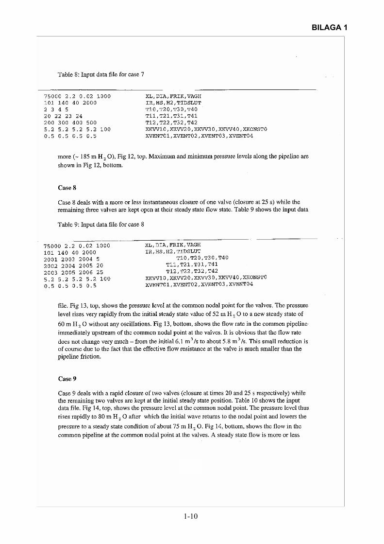
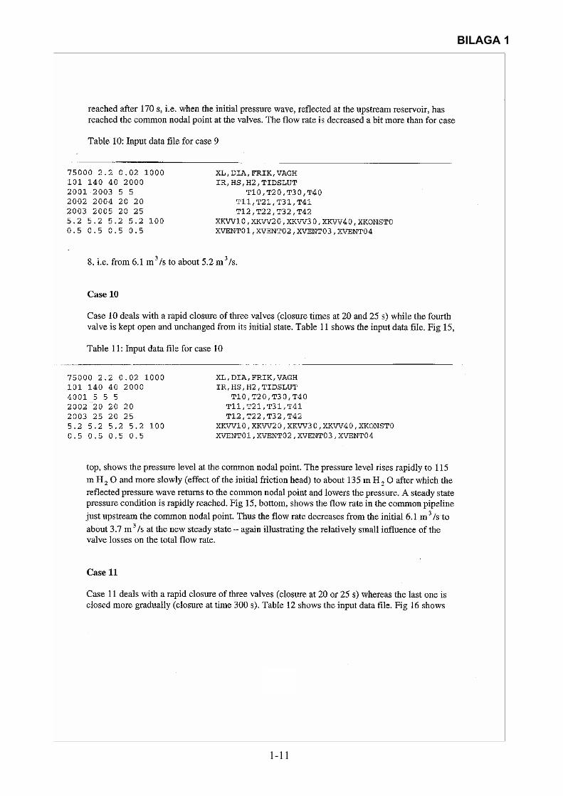
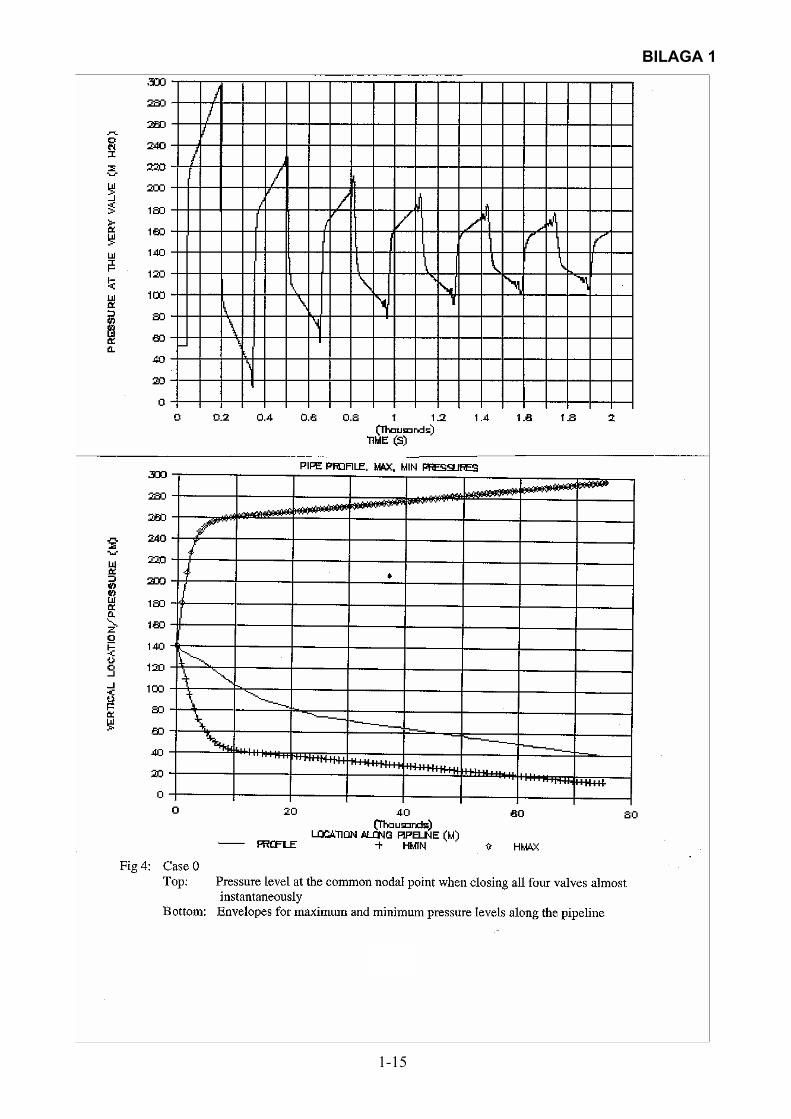
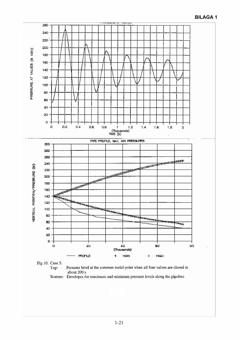
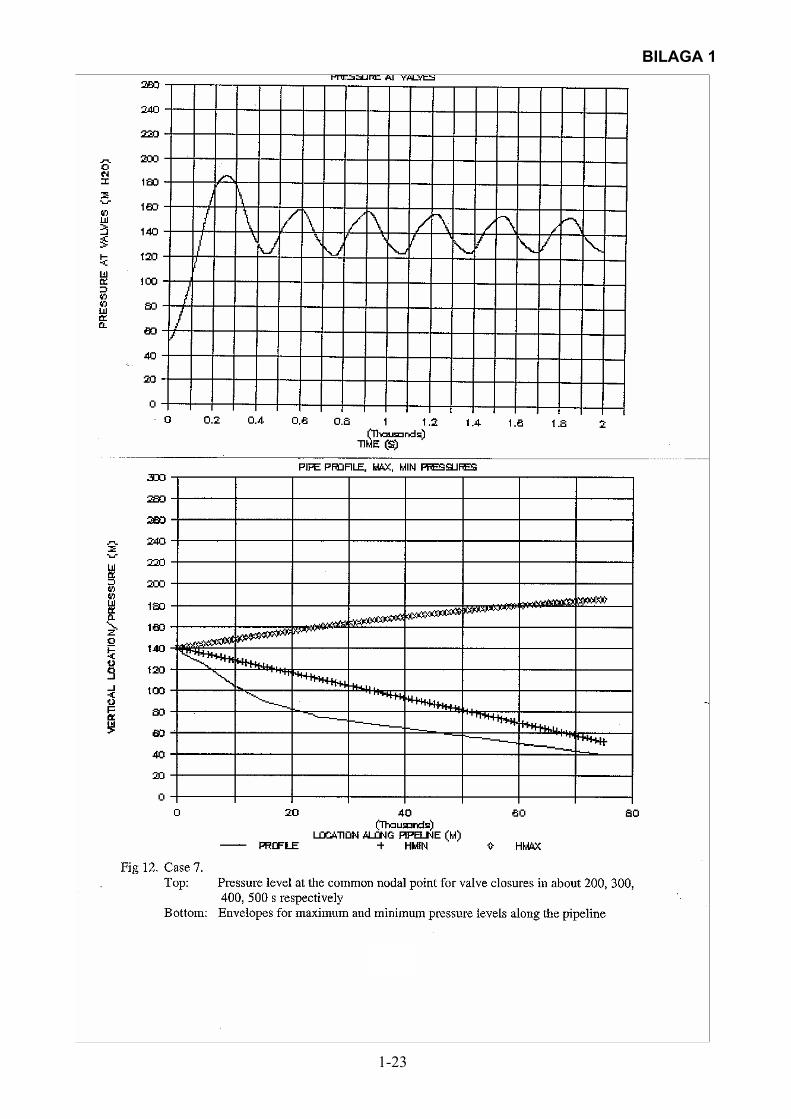
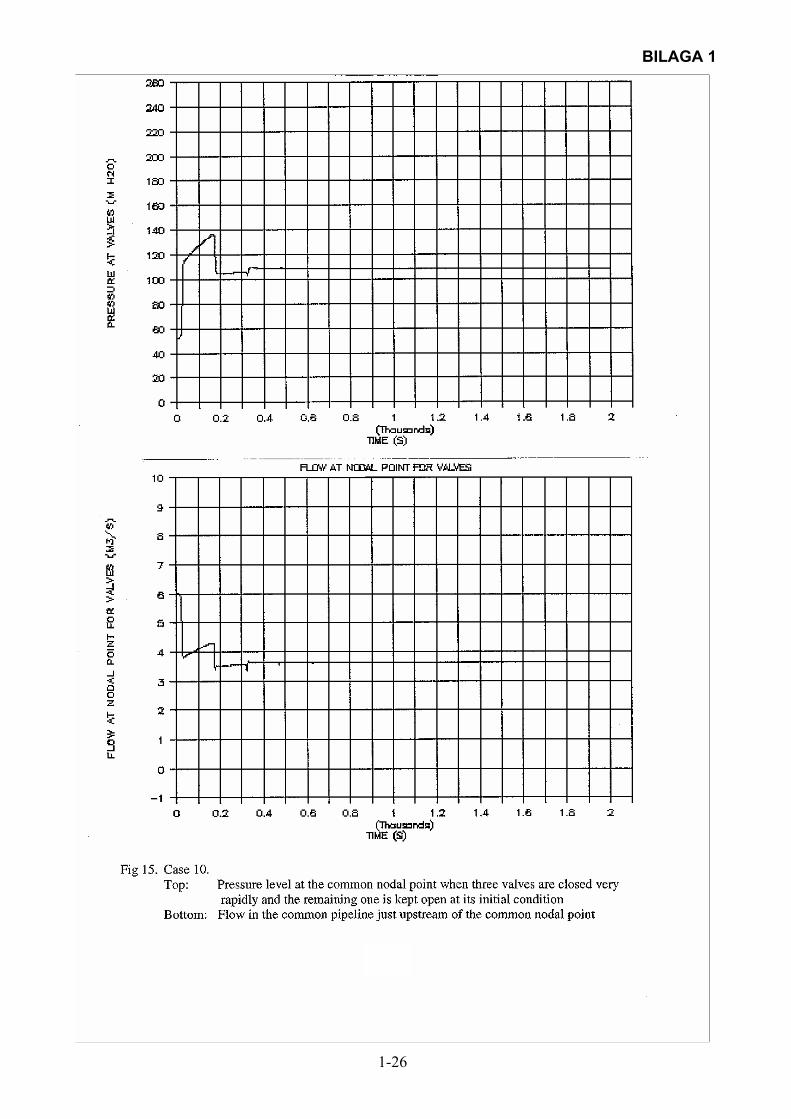
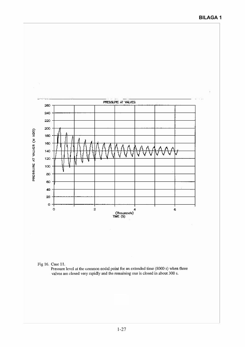
plant. I denna rapport beskrivs ett exempel på ett trycktransientproblem och hur det kan analyseras med beräkningsmodell. Specifikt gällde problemet hur olika stängningsstrategier för fyra parallellkopplade ventiler i slutet av mycket lång ledning från vattenreservoar (tyngdkraftsdriven strömning) påverkade trycktransientförloppen

2. Hydraulic transients in a pipeline with a leak. I denna rapport beskrivs läcksökning

genom analys av trycktransienter i renvattenuppställning i halvstor skala med simulerade läckor. Transienterna åstadkoms med snabb ventilstängning och läckläget bestämdes på grundval av tryckvågsreflexion från läckan samt vågutbredningshastigheten. Numerisk simulering av initiella tryckvågsförloppet gjordes. Läckflöden 5–17 % kunde detekteras med ett absolut medelfel på 1.9 m (ledningslängd c:a 130 m). Olika metoder att bestämma våghastigheten studerades. Spektralanalys tillämpades på teoretiska och experimentella trycktransienter med simulerad läcka. Dock kunde inte en läcka spåras i spektra.

3. Pressure pulsation problems in a sewage water pumping station with a self-evacuating,

centrifugal pump. I denna rapport beskrivs tryckslagsliknande problem i nybyggd pumpstation för avloppsvatten vid normal drift. Snabba, 30–40 Hz, tryckfluktuationer på 10–20 m vattenpelare på trycksidan och 5–10 m vattenpelare på sugsidan konstaterades liksom kavitationsliknande ljud och vibrationer. Ett stort antal dynamiska tryckmätningar utfördes vid befintlig pumpstation liksom efter en rad olika ingrepp (exempelvis åtgärder i pumpsumpen för avluftning, urkoppling av frekvensstyrningen, modifiering av sugledningen) för att förstå och avhjälpa problemen. Det konstaterades att kavitation på sugsidan inte kunde vara orsaken men att problemen var relaterade till luft i pumpen och troligen till dess luftventil. En förbindelse av denna ventil med liten slang till pumpsumpen minskade men eliminerade inte problemen. En intressant iakttagelse var att en grov uppskattning av resonansfrekvensen för luftventilen (membrantyp) var ungefär av samma storlek som tryckvariationernas frekvens.

4. The effect of a gas pocket in a pipeline on hydraulic transients – computer study.

Denna rapport beskriver med hjälp beräkningsexempel hur en lokal gas-/luftficka i en rörledning samverkar med en trycktransient och därmed påverkar transientens utseende. Därmed finns möjlighet att genom analys av en uppmätt tryckvåg få indikation på existens och belägenhet av gasficka. Två signifikanta effekter av fickan kunde utläsas: a) en lågfrekvent trycksvängning uppkom på grund av den periodiska kontraktionen/expansionen för fickan, b) högfrekventa trycksvängningar överlagrades den lågfrekventa svängningen beroende på att tryckvågor fortplantade sig mellan fickan och den stängande ventilen som genererade trycktransienten.

IV

5. Measurements of hydraulic transients in sewage water pumping stations – analysis, wave propagation velocities. I detta projekt presenteras uppmätta trycktransienter i nio olika avloppsvattenpumpstationer med olika ledningsmaterial, med backventil eller avstängningsventil, i något fall med soft start/stop utrustning. Syftet med studien var trefaldigt: 1) insamling av trycktransientdata för operativa förhållanden; 2) kvalitativ analys av trycktransienterna i relation till rörlednings- och pumpstationdata; 3) bestämning av tryckvågshastigheter.

V

SUMMARY Project: Pressure transients in pipelines for water conveyance – problems and benefit The project deals with theoretical, experimental and field studies of hydraulic transients in simple pipelines for the transport of drinking water and sewage water. The transients are generated by start/stop of pumps, valve operation or check valve closure. The conventional view of transients is that they pose a problem as they might damage a pipeline. It is, however, also possible to analyze the appearances of the transients in order to derive some information about the pipelines, for instance concerning the existence and location of a leak or an air pocket. The project has been documented in five reports written in English: 1. Computations of hydraulic transients in raw water pipeline feeding a water treatment

plant. This report describes an example of a hydraulic transient problem and how it could be analyzed using a computational model. Specifically, the problem concerns the issue how different closure strategies of four, parallel valves at the end of a very long pipeline from a water reservoir (gravity driven flow) will affect the hydraulic transients.

2. Hydraulic transients in a pipeline with a leak. This report describes leak detection by

analyzing measured hydraulic transients in a drinking water pilot scale set-up using simulated leaks. The transients were generated by rapid valve closure and the leak location was determined on the basis of the reflection of the pressure wave from the leak and the wave propagation velocity. Successful numerical simulation of the initial pressure wave phase was done. Leak flow rates from 5–17 % could be detected with an absolute average error of 1.9 m (pipeline length 130 m). Different methods for determining the wave velocity were studied. Spectral analysis was applied to theoretical and experimental hydraulic transients with simulated leaks. It was, however, impossible to find any trace of the leak in the spectra.

3. Pressure pulsation problems in a sewage water pumping station with a self-evacuating,

centrifugal pump. This report describes problems of a seemingly hydraulic transient nature in a new pumping station for sewage water from a food industry. Even at steady-state operation, rapid, 30–40 Hz, pressure fluctuations of 10–20 m water column on the pressure side and of 5–10 m water column on the suction side were observed as well as cavitation-like sounds and vibrations. A extensive number of dynamic pressure measurements were performed at the existing pumping station as well as after a number of measures (such as measures in the pump sump for degassing the water, disconnecting the frequency control, modification of the suction pipe) in order to understand and to be able to counteract the problem. It was found that cavitation on the suction side could not be the reason for the problem but that the problem instead was related to air in the pump and to the air vent in the pump. Connecting this vent with the pump sump via a small plastic tube diminished the problem but did not entirely eliminate it. It was observed that a rough estimate of the resonance frequency of the air vent (membrane type) amounted more or less to the same value as the frequency of the pressure fluctuations.

4. The effect of a gas pocket in a pipeline on hydraulic transients – computer study. This

report is based on computational examples and describes how a local gas/air pocket in a pipeline interacts with a hydraulic transient thus affecting the appearance of the transient. In this way there is a possibility to arrive at an indication of the existence and location of the pocket by analyzing a measured transient. Two significant effects of the pocket on the transient were found: 1) a low frequency pressure oscillation occurred due to the periodic contraction/expansion of the pocket; 2) high frequency pressure oscillations were

VI

superimposed on the low frequency oscillation due to the propagation of pressure waves between the pocket and the closing valve, generating the transient.

5. Measurements of hydraulic transients in sewage water pumping stations – analysis,

wave propagation velocities. This report presents measured hydraulic transients in nine different sewage water pumping stations with different pipe material, with check valve or shut-off valves, in a few cases with soft start/stop equipment. The purpose of the study was threefold: 1) gathering of hydraulic transient data for field conditions; 2) qualitative analysis of the transients in relation to data for the pipelines and the pumping stations; 3) determination of pressure wave velocities.

VII

FÖRORD Hydrauliska transienter eller trycktransienter uppkommer i trycksatta ledningar för vattentransport vid snabba flödesförändringar. Därvid uppkommer tryckvågor, som utbreder sig med hög hastighet genom ledningen. Normalt betraktas dessa transienter som ett problem genom att de kan skada ledningen eller dess hydrauliska komponenter. En trycktransient kan emellertid också potentiellt utnyttjas på ett positivt sätt genom att den kan innehålla viktig information om ledningen. En mätning och noggrann analys av en trycktransient har således potentialen att ge indikation om existens och lokalisering av en läcka eller en luft-/gasficka. Även andra ledningsrelaterade egenskaper kan tänkas detekteras – exempelvis dåligt fungerande backventil. Projektet ”Trycktransienter i rörsystem för vattentransport – problem och nytta” har syftat till att belysa båda ovannämnda aspekter på trycktransienter och har rapporterats i fem separata rapporter, som tar upp ett antal aspekter: beräkningsexempel på trycktransienter, experimentell och teoretisk studie av läckinverkan på trycktransient, tryckslagsliknande problem i pumpstation, beräkningsmässig studie av inverkan av luft-/gasficka, mätningar och analyser av trycktransienter från olika typer av pumpstationer. Projektet har ekonomiskt stötts av VA-Forsk och Ångpanneföreningens Forskningsstiftelse, till vilka ett stort tack framförs. Många av mätningarna har kunnat genomföras tack vare ett stort tillmötesgående och beredvillig hjälp från ett stort antal kommuner i Skåne. Jag är mycket tacksam för detta samarbete. Lund 2003-04-09 Lennart Jönsson, Tekn Dr Lunds Tekniska Högskola

VIII

INNEHÅLL Sammanfattning III Summary V Förord VII Sammanfattning av fem rapporter inom projektet: ”Trycktransienter i rörsystem för vattentransport – problem och nytta” 1 Bilaga 1, Computations of hydraulic transients in a raw water pipeline feeding a water treatment plant Bilaga 2, Hydraulic transients in a pipeline with a leak Bilaga 3, Pressure pulsation problems in a sewage water pumping station with a self-evacuating, centrifugal pump Bilaga 4, The effect of a gas pocket in a pipeline on hydraulic transients – computer study Bilaga 5, Measurements of hydraulic transients in sewage water pumping stations – analysis, wave propagation velocities

1

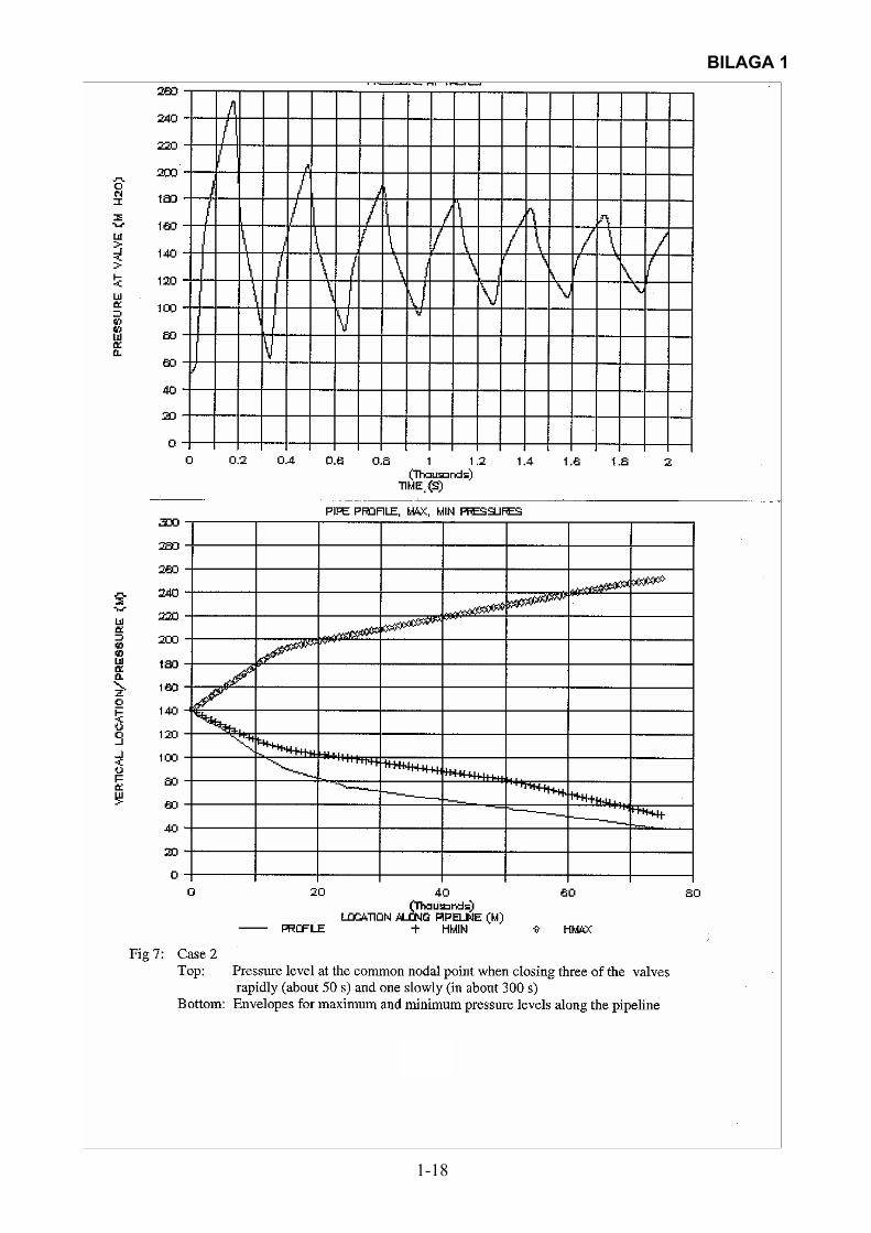
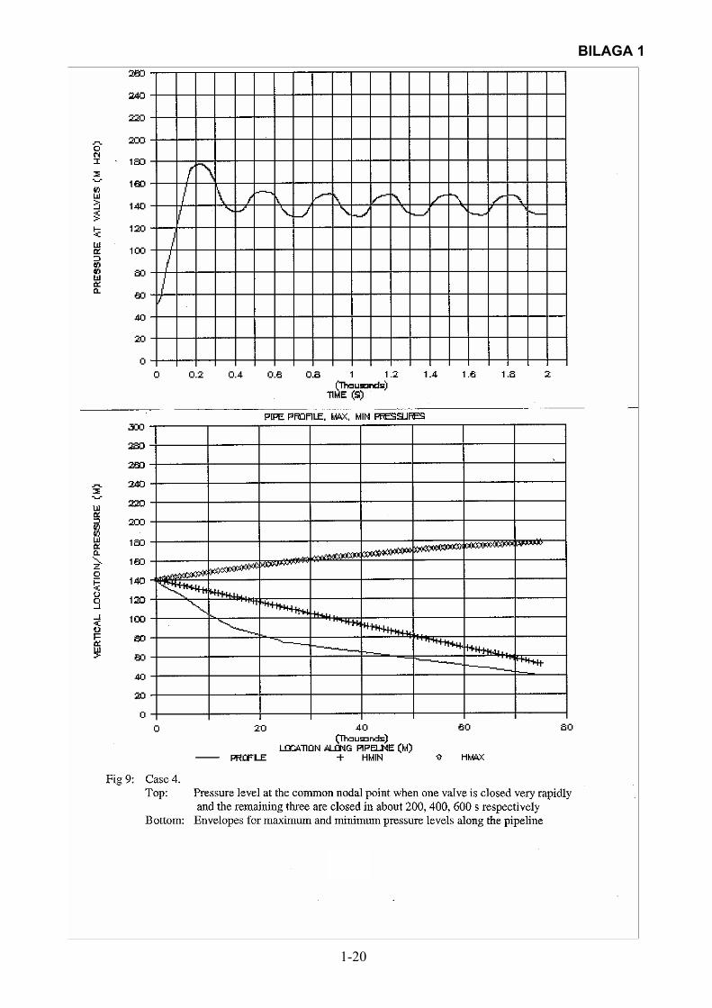
SAMMANFATTNING AV FEM RAPPORTER INOM PROJEKTET: ”Trycktransienter i rörsystem för vattentransport – problem och nytta” 1. Computations of hydraulic transients in a raw water pipeline feeding a water

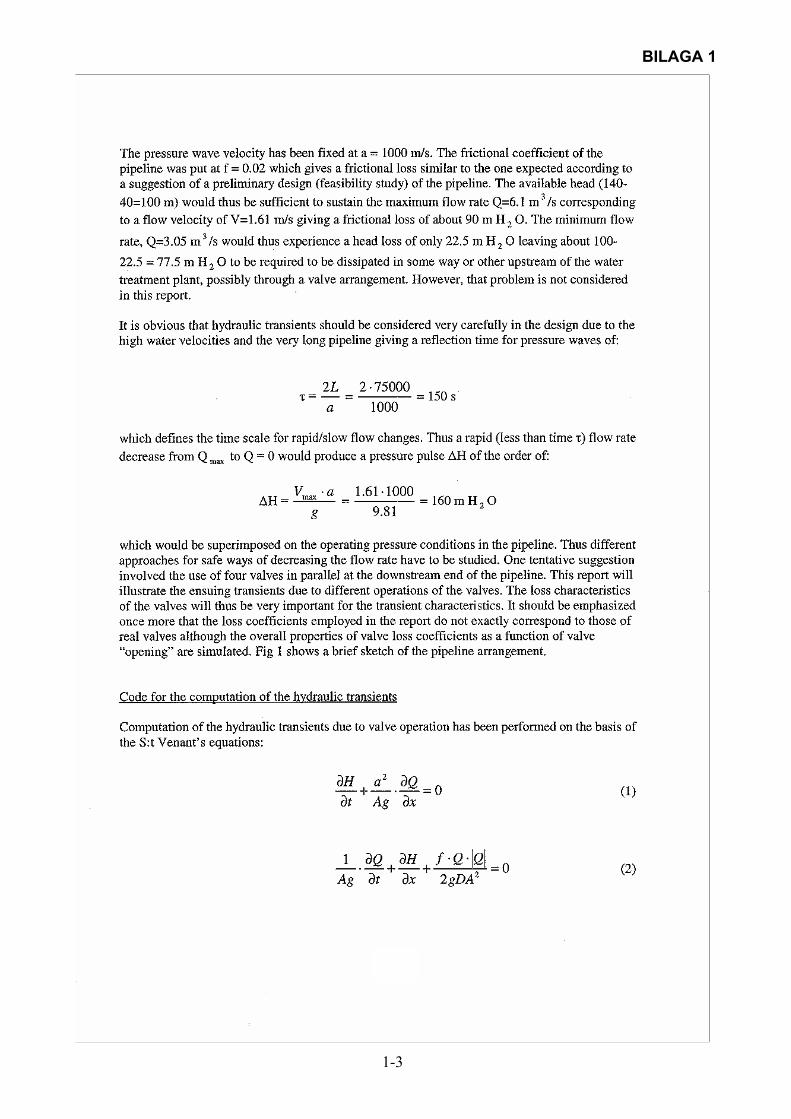
treatment plant. I denna rapport beskrivs ett exempel på ett trycktransientproblem och hur det kan analyseras med beräkningsmodell. Specifikt gäller det beräkning av de hydrauliska transienterna, som uppkommer i en mycket lång rörledning med tyngdkraftsdriven strömning från en vattenreservoar till ett vattenverk och där flödesändringen åstadkoms genom ventilmanövrering av fyra parallellkopplade avstängningsventiler i ledningens nedströmsände. Ventilmanövreringen illustrerades genom att ventilerna stängdes på olika sätt – snabb stängning av alla ventilerna, långsam stängning av alla ventilerna, en eller flera snabbt och resterande en eller flera långsamt. Syftet med rapporten var att illustrera sambandet mellan de hydrauliska transienternas egenskaper och ventilmanövreringen för ett fall där ledningsfriktionen var mycket betydande. Det främsta intresset var fokuserat på maximaltrycken på grund av dess betydelse för ledningens hållfasthet. Det kunde emellertid också noteras att det s.k. ”line packing” fenomenet var mycket markant. Detta senare innebär att friktionen transformeras till en ytterligare, relativt långsam tryckökning utöver den initiella tryckökningen, då tryckvågen från en stängande ventil utbreder sig genom röret. Det framkom också att om åtminstone en ventil hålls öppen under en även snabb ventilstängningsoperation i ventilsystemet, så påverkas flödet i relativt ringa grad. Detta leder i sin tur till små trycktransienter. Slutligen så visade beräkningarna också att en transient strömningssituation kommer att fortleva långt efter det att fullständig ventilstängning har uppnåtts. 2. Hydraulic transients in a pipeline with a leak. I denna rapport beskrivs experimentella och teoretiska studier avseende samverkan mellan en hydraulisk transient i en rörledning och en simulerad läcka med speciell tonvikt på möjligheten att upptäcka och lokalisera läckan genom noggrann analys av transienten. Den grundläggande idén är att en brant och kraftig tryckvåg, genererad exempelvis genom ventilstängning eller pumpstopp, delvis kommer att reflekteras i läckpunkten och kan spåras i trycktransientmätningen. En kunskap om tryckvågshastigheten och tillryggalagd tid för den reflekterade vågen tillbaka till mätpunkten möjliggör en uppskattning av läget för läckan. Experiment har tidigare utförts på röruppställning med en snabb avstängningsventil i nedströmsänden. Ventilstängningen genererade en brant tryckvåg, vilken registrerades med dynamisk tryckgivare. Effekten av simulerade läckor vid två lägen uppströms om läckan undersöktes. I ett av fallen med en läcka 42.85 m uppströms ventilen kunde en markant effekt av läckan noteras såsom en abrupt förändring (minskning) av trycket. Den simulerade läckan vid 79.65 m var svår att upptäcka, huvudsakligen beroende på den möjliga effekten av en flexibel 900:s krök, vilken maskerade läckeffekten. Våghastigheterna bestämdes på olika sätt, på grundval av reflektionstiden från huvudledningen (fungerade som reservoar), på grundval av den initiella tryckstegringen enligt Kutta-Joukowski’s lag, på grundval av det oscillerande tryckets periodtid efter ventilstängning, samt på grundval av teoretisk formel. Det befanns att den förstnämnda metoden var det mest lämpade för de aktuella mätningarna. Den tredje metoden (baserad på oscillerande trycket) visade alltför låg våghastighet, troligen beroende på att mycket små mängder gasbubblor löstes ut under undertrycksfaser. För läckan vid 42.85 m befanns att läckflöden i intervallet 5–17 % kunde lokaliseras med ett absolutfel i medeltal om 1.9 m (ledningslängd 130 m). I några fall kunde också läckan vid 79.65 m lokaliseras med god noggrannhet.

2

Numerisk simulering på basis av St Venant’s 1-d instationära, kompressibla strömningsekvationer utfördes för att simulera den initiella fasen för de uppmätta trycktransienterna. Speciell tonvikt lades vid möjligheten att beskriva läckeffekten utan att ta hänsyn till den något flexibla 900:s kröken. En kvalitativt god överensstämmelse med uppmätta trycktransienter erhölls med avseende på läckeffekten. Detta faktum indikerar att beskrivningen av läckan i beräkningarna var acceptabel. Spektralanalys med FFT (Fast Fourier Transform) teknik gjordes på både teoretiskt beräknade trycktransienter och på uppmätta trycktransienter – i båda fallen med simulerad läcka. Avsikten var att undersöka om en läcka gav upphov till snabbare trycksvängningar under den transienta fasen och vilka skulle kunna kopplas till läckan för lokaliseringsändamål. Tyvärr kunde inte någon sådan topp i spektra hittas, varken för de teoretiska eller de uppmätta transienterna. Således befanns inte spektralanalys vara ett användbart instrument för läcklokalisering. 3. Pressure pulsation problems in a sewage water pumping station with a self-evacuating,

centrifugal pump En ny pumpstation erhåller avloppsvatten från en livsmedelsindustri för vidare transport till reningsverk via ytterligare pumpstationer. Pumpstationen, som är utrustad med två självevakuerande centrifugalpumpar med sughöjd om 2–3 m, har haft problem alltsedan starten. Dessa problem yttrade sig som tryckändringar både på sug- och trycksidan hos vardera pumpen i pumpstationen. Tryckfluktuationerna kunde uppgå till 10–20 m vattenpelare på trycksidan och 5–10 m på sugsidan beroende på flödets storlek. Dessutom åtföljdes pumpdrift av starkt buller och vibrationer, det förra påminnande om kavitation. För att finna orsaken till det onormala uppförandet hos pumparna utfördes högfrekventa, dynamiska tryckmätningar. Resultaten från dessa mätningar, relaterade till andra tester, observationer och tänkbara motåtgärder, diskuteras i denna rapport. Vanlig kavitation med ångblåsor på grund av lågt tryck på sugsidan uteslöts som orsak till problemen. Istället framfördes en rad hypoteser – resonans på grund av styrsystemet för frekvenskontroll, fysisk skada på pumphjulen, olämplig utformning av sugsidans rör och/eller pumpsumpen, gas/luft i avloppsvattnet, illa fungerande luftventil i själva pumpen, inverkan av tryckledningen. Transienta tryckmätningar och/eller visuella observationer utfördes på basis av nämnda hypoteser och för olika pumpdriftfall och den slutsatsen drogs att pumpproblemen var relaterade till befintligheten av luft-/gasbubblor i pumpen trots att dessa senare inte tycktes vara orsakade av pumpsumpen, avloppsvattnet eller sugsidans rör. Mätningarna visade att tryckfluktuationer uppstod mer eller mindre för alla motorfrekvenser 0–50 Hz, men att fluktuationerna var speciellt starka och regelbundna för motorfrekvenser om c:a 38–40 Hz. Ett intressant resultat var att en grov uppskattning av resonansfrekvensen (44 Hz) för luftventilen av membrantyp överensstämde väl med ovannämnda frekvensintervall 38–40 Hz. En förbindelse av luftventilen med pumpsumpen med en tunn plastslang visade sig delvis framgångsrik genom att tryckfluktuationerna på sugsidan försvann nästan helt. Slutsatsen av studien var att orsaken till pumpproblemen inte blev fullständigt klarlagd. Det tycktes emellertid som om en viktig del till förklaringen låg i befintligheten av luft/gas i pumpen. Källan till luften/gasen har inte fullt ut klarlagts men flera omständigheter indikerar att luftinträngning är kopplad till luftventilen. 4. The effect of a gas pocket in a pipeline on hydraulic transients – computer study

Mätning och noggrann analys av trycktransienter i ledningar för vattentransport kan ge värdefull information om några aspekter på rörledningen och dess hydrauliska egenskaper. En sådan aspekt gäller befintligheten av begränsade luft-/gasfickor i rörledningen, vilka kan påverka kapaciteten

3

samt orsaka instationära flödesförhållanden. Avsikten med denna rapport är att undersöka effekten av en luftficka på egenskaperna hos en trycktransient i en enkel, 1000 m lång ledning. Studien utfördes med ett antal beräkningsexempel på grundval av de 1-d, instationära, kompressibla strömningsekvationerna (St Venant’s ekvationer) lösta med karakteristikmetoden. De numeriska exemplen avsåg tyngdkraftdriven strömning i en enkel rörledning, som förenade två reservoarer och med en avstängningsventil i nedströmsdelen av ledningen. Hydrauliska transienter genererades genom stängning av ventilen. Luftfickans storlek och läge varierades. En jämförelse med hydraulisk transient i fallet utan luftficka visade att denna generellt hade stor inverkan på den hydrauliska transientens utseende. Man kunde urskilja två stora effekter, förutsatt att fickan inte var alltför liten:

- en lågfrekvent trycksvängning uppkom på grund av periodisk kontraktion/expansion hos luftfickan

- en högfrekvent trycksvängning överlagrades den lågfrekventa trycksvängningen

beroende på att tryckvågor utbredde sig mellan den stängda ventilen och luftfickan. Möjligheten att erhålla ovan nämnda två effekter tycktes bero på fickans läge, utöver (naturligtvis) fickans storlek. Sålunda befanns:

- för luftfickläge 250 m från uppströmsänden av ledningen kunde man observera effekten av luftfickan ned till en ficklängd om c:a 2.5 m

- för luftfickläge 500 m från uppströmsänden av ledningen kunde man observera

effekten av luftfickan ned till en ficklängd om c:a 0.25 m

- för luftfickläge 750 m från uppströmsänden av ledningen kunde man observera effekten av luftfickan ned till en ficklängd om c:a 0.025 m.

Amplituden för de högfrekventa trycksvängningarna, som berodde på tryckvågsutbredning mellan ventilen och luftfickan, avtog med ökande avstånd från ventilen till luftfickan och med minskande storlek på luftfickan. Studien visar således, att användning av hydrauliska transienter som en ”mätprobe” för en enkelledning kan indikera befintlighet av en luft-/gasficka genom en noggrann analys av transienten. För det första ger luftfickan upphov till ganska lågfrekventa trycksvängningar med typiska, spetsiga toppar och mer avrundade dalar. För det andra, under förutsättning att tillräckligt stor reflektion av tryckvågor äger rum vid fickan, bör det också vara möjligt att lokalisera (åtminstone ungefärligt) fickan på basis av periodtiden för de högfrekventa trycksvängningarna och våghastigheten. 5. Measurement of hydraulic transients in sewage water pumping stations – analysis,

wave propagation velocities Denna rapport presenterar data om hydrauliska transienter, som har uppmätts i nio olika rörledningar för transport av kommunalt avloppsvatten. Alla mätningarna har utförts i pumpstationerna och transienterna har genererats genom start/stopp av en eller två pumpar. Rörlängderna varierade mellan 748 m och 3240 m. Rörmaterialet varierade: gjutjärn (1), delvis gjutjärn och delvis PVC (1), PVC (4), PE (2), PEH (1). Pumpstationerna var utrustade med backventiler eller avstängningsventiler. I de flesta fallen innebar pumpstoppet ett omedelbart tryckfall på grund av litet tröghetsmoment hos pumpen. I något fall var pumparna utrustade utrustning för mjukstart, -stopp vilket innebar att stopp-/startproceduren skedde gradvis genom frekvenskontroll.

4

Syftet med studien var trefaldigt: 1) att samla in trycktransientdata under operationella förhållanden, 2) att analysera utseendena hos de hydrauliska transienterna kvalitativt och kvantitativt och att relatera transienternas egenskaper till ledningens och pumpstationens egenskaper, 3) att härleda tryckvågshastigheter på basis av mätningarna. 30 olika mätningar av hydrauliska transienter visas och diskuteras. Maximi- och minimitryck bestämdes men i inget fall befanns dessa vara onormalt höga eller låga. De hydrauliska transienternas utseenden kunde i de flesta fallen förklaras på grundval av ledningsegenskaper och det sätt de hydrauliska komponenterna manövrerades. Således kunde man tydligt observera det initiella tryckfallet vid pumpstopp, den därpå följande backventilstängningen och de regelbundna trycksvängningar som uppkom efter ventilstängning genom att tryckvågor utbredde sig fram och tillbaka mellan den stängda ventilen och rörledningens öppna nedströmsdel. Mjukstart eller –stopp ändrade den initiella fasen hos den hydrauliska transienten. Sålunda avtog trycket mer gradvis i jämförelse med fallet utan mjukstopp. Det var möjligt att i en pumpstation jämföra effekten av mjukstopp och icke-mjukstopp. Därvid befanns att skillnaden i maximitryck och minimitryck i de två fallen var mycket liten, vilket med stor sannolikhet berodde på att tidsskalan för mjukstoppet var för liten. Tryckvågshastigheter bestämdes på basis av mätningarna – antingen med utgångspunkt från periodtiden för de regelbundna trycksvängningarna eller från tidsperioden för en tryckvåg att utbreda sig fram och tillbaka en gång i röret (initiellt). Dessa våghastigheter jämfördes också med teoretiskt beräknade dylika. Det befanns att i de flesta fallen avvek uppmätta våghastigheter signifikant från de teoretiska. I de fall där flera uppskattningar av våghastigheten kunde göras för en viss ledning (antingen med olika transientmätningar eller med olika metoder på en och samma mätning) befanns att hastigheterna var mycket snarlika. Därför rekommenderas, om möjligt, användning av tryckvågshastigheter genom direkt analys av uppmätta trycktransienter för en specifik ledning i fall där våghastigheten bör vara känd med så stor noggrannhet som möjligt.

BILAGA 1

BILAGA 1

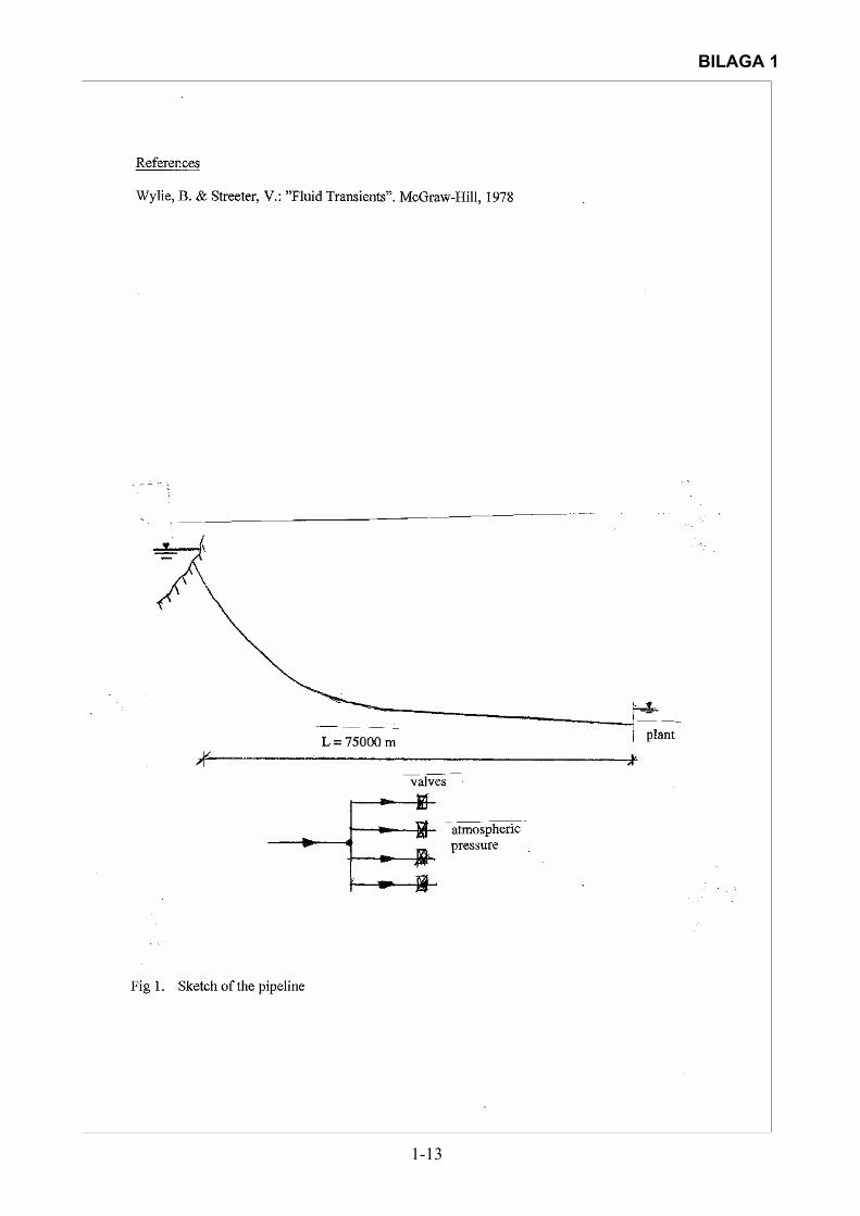
CONTENTS page Abstract......................................................................................................... 1-1 Acknowledgement ........................................................................................ 1-1 Introduction .................................................................................................. 1-2 Pipeline characteristics ................................................................................. 1-2 Code for the computation of hydraulic transients ........................................ 1-3 Results .......................................................................................................... 1-6 Discussion and conclusion ......................................................................... 1-12 References .................................................................................................. 1-13 Figures 1–16 ............................................................................................... 1-13 Appendix Fortran program ......................................................................... 1-28

BILAGA 1

1-1

BILAGA 1

1-2

BILAGA 1

1-3

BILAGA 1

1-4

BILAGA 1

1-5

BILAGA 1

1-6

BILAGA 1

1-7

BILAGA 1

1-8

BILAGA 1

1-9

BILAGA 1

1-10

BILAGA 1

1-11

BILAGA 1

1-12

BILAGA 1

1-13

BILAGA 1

1-14

BILAGA 1

1-15

BILAGA 1

1-16

BILAGA 1

1-17

BILAGA 1

1-18

BILAGA 1

1-19

BILAGA 1

1-20

BILAGA 1

1-21

BILAGA 1

1-22

BILAGA 1

1-23

BILAGA 1

1-24

BILAGA 1

1-25

BILAGA 1

1-26

BILAGA 1

1-27

BILAGA 1

1-28

BILAGA 1

1-29

BILAGA 1

1-30

BILAGA 1

1-31

BILAGA 1

1-32

BILAGA 1

1-33

BILAGA 1

1-34

BILAGA 1

1-35

BILAGA 2

DEPARTMENT OF WATER RESOURCES ENGINEERING LUND INSTITUTE OF TECHNOLOGY, LUND UNIVERSITY

CODEN:LUTVDG/(TVVR-3236)/1-95(2001)

HYDRAULIC TRANSIENTS IN A PIPELINE WITH A LEAK

by

Lennart Jönsson

The research reported in this document has been made possible through the sponsorship by Ångpanneföreningens Forskningsstiftelse, Stockholm, Sweden and by VA-Forsk, Stockholm,

Sweden

BILAGA 2

CONTENTS page Abstract......................................................................................................... 2-1 Acknowledgement ........................................................................................ 2-1 Introduction .................................................................................................. 2-2 Effect of a leak on a hydraulic transient – general discussion...................... 2-2 Experimental set-up...................................................................................... 2-3 Analysis of the transients – methodologies, general description.................. 2-5 Location of a leak based on the reflected wave.............................. 2-5 Numerical simulation of the leak effect on a transient................... 2-9 Spectral analysis ........................................................................... 2-11 Pressure transient measurements ................................................................ 2-12 Brief comments on some of the individual transient measurements ............................................................................................. 2-13 Determination of leak location according to the reflected transient wave.............................................................................. 2-18 Numerical simulation of the effect of a leak on the transient..................... 2-19 Spectral analysis of transients .................................................................... 2-24 FFT analysis on computed transients ........................................... 2-25 FFT analysis on measured transients............................................ 2-26 Conclusions ................................................................................................ 2-27 References .................................................................................................. 2-29 Figures ........................................................................................................ 2-30 Appendix 1, computer program for transient

calculations in a pipeline with a leak..................................................... 2-87 Appendix 2, computer program for FFT analysis ...................................... 2-92

BILAGA 2

2-1

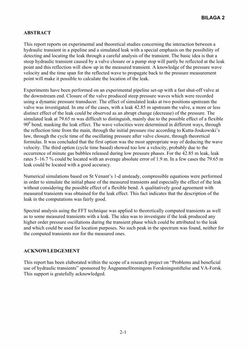
ABSTRACT This report reports on experimental and theoretical studies concerning the interaction between a hydraulic transient in a pipeline and a simulated leak with a special emphasis on the possibility of detecting and locating the leak through a careful analysis of the transient. The basic idea is that a steep hydraulic transient caused by a valve closure or a pump stop will partly be reflected at the leak point and this reflection will show up in the measured transient. A knowledge of the pressure wave velocity and the time span for the reflected wave to propagate back to the pressure measurement point will make it possible to calculate the location of the leak. Experiments have been performed on an experimental pipeline set-up with a fast shut-off valve at the downstream end. Closure of the valve produced steep pressure waves which were recorded using a dynamic pressure transducer. The effect of simulated leaks at two positions upstream the valve was investigated. In one of the cases, with a leak 42.85 m upstream the valve, a more or less distinct effect of the leak could be observed as an abrupt change (decrease) of the pressure. The simulated leak at 79.65 m was difficult to distinguish, mainly due to the possible effect of a flexible 900 bend, masking the leak effect. The wave velocities were determined in different ways, through the reflection time from the main, through the initial pressure rise according to Kutta-Joukowski’s law, through the cycle time of the oscillating pressure after valve closure, through theoretical formulas. It was concluded that the first option was the most appropriate way of deducing the wave velocity. The third option (cycle time based) showed too low a velocity, probably due to the occurrence of minute gas bubbles released during low pressure phases. For the 42.85 m leak, leak rates 5–16.7 % could be located with an average absolute error of 1.9 m. In a few cases the 79.65 m leak could be located with a good accuracy. Numerical simulations based on St Venant’s 1-d unsteady, compressible equations were performed in order to simulate the initial phase of the measured transients and especially the effect of the leak without considering the possible effect of a flexible bend. A qualitatively good agreement with measured transients was obtained for the leak effect. This fact indicates that the description of the leak in the computations was fairly good. Spectral analysis using the FFT technique was applied to theoretically computed transients as well as to some measured transients with a leak. The idea was to investigate if the leak produced any higher order pressure oscillations during the transient phase which could be attributed to the leak and which could be used for location purposes. No such peak in the spectrum was found, neither for the computed transients nor for the measured ones. ACKNOWLEDGEMENT This report has been elaborated within the scope of a research project on “Problems and beneficial use of hydraulic transients” sponsored by Ångpanneföreningens Forskningsstiftelse and VA-Forsk. This support is gratefully acknowledged.

BILAGA 2

2-2

INTRODUCTION Hydraulic transients (waterhammer, pressure transients) occur in completely filled pipelines for water conveyance at rapid flow changes due to pump stop, valve closure etc. At the location of the flow change pressure waves are generated and which propagate back and forth in the pipeline until dissipation mechanisms have attenuated the waves completely and a new steady state flow condition (for instance zero flow) has been reached. Normally, the phenomenon of hydraulic transients is considered a problem as the pressure waves could pose a risk for the strength and functioning of the pipeline – i.e. strong pressure peaks might make the pipeline burst, periods of low pressure might cause buckling and the oscillatory nature of the pressure waves will give rise to fatigue problems. However, hydraulic transients might also be used in a beneficial way. This is due to the fact that a hydraulic transient is a wave propagating through the pipeline. Generally speaking the nature and appearance of a transient will depend on a number of factors some of them determining the overall properties or characteristics of the transient. This category of factors could indicate the pipe length, the pipe material, the way the flow is changed. There are, however, also a number of factors with often less importance and which will influence modify the appearance of the transient. Examples of such factors are given by a small leak, an air pocket, change of pipe diameter, branching of a pipeline. Thus, a hydraulic transient could be considered as a “probe” propagating through the pipeline from its place of generation. The basic idea of using a transient as a tool for obtaining information on some hydraulic (or other kinds of) properties of a pipeline will thus be to generate a transient in a controlled way, to measure the transient and to analyze it carefully in order to understand the appearance of the transient and to relate it to properties of the pipeline. One application of the above-mentioned general idea is to try to detect and locate leak(s) in a pipeline system. The purpose of this report is to describe and analyze measurements of hydraulic transients on an experimental set-up of a pipeline with simulated leaks. The effect of different leakage rates on the appearance of the transients will be discussed as well as the possibility to locate the leak. Moreover, a computational model of the transients will be applied in order to investigate the possibility to describe the effect of a leak theoretically. Finally, the spectral properties of transients will be studied using the Fast Fourier Transform technique (FFT) as one might put forward the hypothesis that an analysis of a spectrum might provide an alternative way of studying leaks on the basis of transients. EFFECT OF A LEAK ON A HYDRAULIC TRANSIENT – GENERAL DISCUSSION Consider a single pipeline, length L, with a pumping station equipped with a check valve at the upstream end and a reservoir at the downstream end , Fig 1. Assume that a leak is located at a distance L1 from the pumping station. The velocity of pressure waves (the transient) is a. Dynamic pressure measurements are performed immediately downstream of the valve. At steady state operation a certain pressure head H0 prevails at the pump, Fig 2. Stopping the pump produces a very steep (more or less instantaneous) pressure drop to about atmospheric pressure provided the inertia of the pump is not too high, a condition, which normally is fulfilled. This pressure drop propagates towards the leak with the wave velocity a. A part of the pressure wave will be reflected at the leak, the amount of reflection depending on the size of the leak. For a small leak most of the pressure wave will propagate further downstream, being reflected at the downstream reservoir. The reflected

BILAGA 2

2-3

pressure wave at the leak will propagate upstream and reach the dynamic transient measurement point after a certain time ∆t after pump stop. This will affect the transient measurement, theoretically causing the pressure trace to experience a small “bump”, see Fig 2 lower part. Knowledge of the time ∆t and the wave velocity a makes it possible to calculate the location of the leak 1L :

2

taL1∆⋅

= (1)

The main part of the pressure wave will propagate back and forth through the pipeline and eventually the check valve will close when the water velocity at the valve has been reduced to zero. The subsequent transient pressure measurement will be characterized by an oscillating behaviour with time period T according to the relation:

aL4T ⋅

= (2)

The presence of the leak will also affect the pressure trace as a certain, higher frequency distortion of the basic, very regular oscillatory signal after valve closure. Another effect of the leak is that the amplitude of the oscillatory pressure variation will decrease more rapidly than for the equivalent flow case without a leak where friction is the sole energy dissipation factor. The effect of the leak on the hydraulic transient has been discussed for a specific case, i.e. pump stop in a single pipeline. The same effect would in principle occur in a pipeline where the transient is generated through a valve closure. Thus, it has been discussed that the existence of a leak in a single, homogeneous pipeline will manifest itself in different ways:

- as a small pressure change where one normally would not expect it - as a superposition of higher frequency disturbances on the basic, regular oscillatory

pressure behaviour after valve closure - as an unusually rapid attenuation of the pressure waves.

Moreover, the location of the leak could be determined on the basis of a knowledge of the wave velocity and the arrival time to the measurement point of the reflected wave from the leak. EXPERIMENTAL SET-UP Measurements of the effect of a simulated leak on a hydraulic transient have been performed on an experimental set-up (Jönsson et al 1997) at the Bulltofta Waterworks in Malmö. A sketch of the set-up is shown in Fig 3. The upstream end of the pipeline was connected to a water main with a pressure of about 5 bar above the atmospheric pressure. This main worked as a reservoir, i.e. defining a constant pressure vessel of a sufficiently large volume during each of the transient measurements. The pipeline itself basically consisted of two parts – one 35.9 m long and one 98.35 m long – separated by a 90 o smooth elbow, i.e. a total length of the pipeline of very close to 135 m. The downstream end of the pipeline discharged to the atmosphere via a ball valve which could be manually operated very fast. The 35.9 m part consisted a galvanized steel pipe, inner diameter 41.8

BILAGA 2

2-4

mm and wall thickness 3.25 mm and the 98.35 part consisted of a galvanized steel pipe either inner diameter 53 mm, wall thickness 3.65 mm (measurement nr BULL32 or less) or inner diameter 41.8 mm, wall thickness 3.25 mm (measurement nr BULL46 or larger). A turbine type of a flow meter was located immediately downstream of the o90 bend. Three simulated leaks were located at 15.15 m, 42.85 m and 79.65 m respectively upstream from the ball valve. Each leakage point consisted of a T-joint with a valve and a flow meter on the very short “leakage leg” of the joint. Only one leak was operational at each measurement. Pressure transients were obtained by rapid ball valve closure. Measurements of the transient pressure were performed at the ball valve by means of a dynamic pressure transducer – mark TransInstruments – with an upper frequency response of 25 Hz with a sampling frequency of 640 Hz. The analogue transducer signals were A/D converted, amplified and transformed into pressure units using an ABC computer. Calibration relied on measurements of the atmospheric pressure and of the stable (and checked) characteristics of the pressure transducer. In order to facilitate the further description of the analysis of the hydraulic transient measurements an example of the recordings will briefly be discussed with reference to Figs 4a, 4b (measurement BULL12, i.e. 53 mm pipeline). Q pipeline = 0.80 l/s and Q leak = 0.04 l/s, i.e. the leak flow is 5 % of the pipeline flow upstream the leak. The simulated leak was located at 42.85 m upstream of the ball valve. Fig 4a shows the entire pressure trace at rapid ball valve closure with an initial pressure rise, which should correspond to the Kutta-Joukowski law provided the valve closure could be considered instantaneous:

OHmg

VaH 2∆⋅

=∆ (3)

where ∆H = pressure change ∆V = change of water velocity g = 9.81 m/s 2 The generated pressure waves propagate back and forth through the entire pipeline between the valve and the main giving rise to the cyclic behaviour of the pressure. A small part of the pressure wave is reflected each time when passing the leak thus causing a somewhat distorted oscillatory appearance. One also notices the attenuation of the pressure waves, partly due to the leak flow. Fig 4b shows a close-up of the initial pressure rise. In the first place one notices the steep rise of the pressure due to the rapid valve closure. After that the pressure rises much more slowly due to the “line-packing” effect, i.e. the influence of pipeline friction as the initial pressure rise propagates downstream the pipeline. However, after a certain time (at about time t= 3.04 s) the pressure starts to decrease slightly. This is the effect of the reflection of the initial positive pressure wave at the leak and now reaching the pressure transient measurement point. The time ∆t which has elapsed from the start of the pressure rise to this break in the rising pressure trend is a measure of the location of the leak. The passage of the initial steep pressure wave at the leak will produce increasingly stronger reflected pressure which, reaching the measurement point, will continue to decrease the pressure there, theoretically during the same duration as for the initial steep pressure rise. After that the pressure at the measurement point should be more or less constant as the corresponding pressure wave passing the leak has got an approximately constant amplitude. There is thus a “plateau” of a rather short duration in the pressure trace, at about time t= 3.08 s. One would expect that the measured pressure would remain at this constant level (beside small frictional line-packing effects) until the initial pressure wave has been reflected at the main and returned to the measurement point. There is, however, a weak undulation of the pressure after about time t=3.08 s. Moreover, one could observe a substantial rise in the pressure just before t=3.2 s which is higher

BILAGA 2

2-5

than what one would expect from frictional effects. The most probable reason for these two “abnormalities” is the existence of the 90 o -bend being slightly flexible (Wood et al 1971). Thus, the closure of the valve would give rise to a “precursor” tensile wave propagating in the pipe wall itself and with a wave velocity which is significantly higher than the normal hydraulic transient wave velocity. This precursor wave will interact with the flexible bend moving it initially in the ball valve direction. At about time t=3.15 s the pressure trace changes character slightly from a slowly changing pressure to a faster changing pressure. This situation is interpreted as the reflection of the normal hydraulic transient wave at the 90 o bend and having returned to the pressure measurement point. At about time t=3.2 s the pressure drops rapidly due to the fact that the initial pressure wave has returned to the pressure transducer after reflection at the main. One might argue that the significant pressure rise just before time t=3.15 s is due to the change in pipe diameter. However, more or less the same phenomenon was observed for the experimental cases with the same kind of pipe (diameter 41.3 mm) throughout the whole pipeline. A third possibility for the pressure rise at about time t=3.2 s is the effect of added elasticity because of the flow meter in the pipeline at location 98.5 m. This approach was used in the numerical simulations. The results of this latter approach were, however, not conclusive. ANALYSIS OF THE TRANSIENTS – METHODOLOGIES, GENERAL DESCRIPTION The measured transients were primarily analyzed as to the location of the simulated leak by identifying (if possible) the reflected wave from the leak due to the passage of the initial pressure wave generated through valve closure. Secondly, the possibility of computational simulation of the effect of the leaks on the measured transients was investigated. Thirdly, application of FFT analysis on transients in leakage situations was studied in order to investigate a possible relation between a leak location and the spectral properties. In this chapter the above-mentioned three aspects will be discussed in general terms, LOCATION OF A LEAK BASED ON THE REFLECTED WAVE Determination of the location of a leak based on the reflection of the initial pressure waves is based on Eq(1). Thus, two entities should be determined, the pressure wave velocity a and the time ∆t. An accurate evaluation of ∆t from the measured pressure trace requires two things, a well-defined start of the pressure change (in our case the valve closure) and a well-defined appearance of the reflected wave on the recorded pressure transient. Generally speaking one could assume that the more rapid (steep) and the stronger the pressure change is the more accurate will the determination of ∆t be. Thus, it is important to close the valve rapidly as far as the experiments on the set-up are concerned. Another, and very common situation in practice concerns a pipeline with a pump. Switching off the power to a running pump will generate a very rapid decrease of the pressure at the pump, a well-defined negative wave which will partly be reflected at a leak and which will produce a small “bump” of the pressure trace, similar to the valve closure case. This is true provided that the inertia of the pump is small which is the normal case. If the pump is equipped with a soft stop arrangement or if the pump is connected to an air vessel (or surge shaft) disconnection of such devices has to be done in order to produce an appropriate transient. In such a case care should of course be taken not to damage the pipeline. The transient measurements, which were performed at the experimental set-up, were done with sampling frequency of 640 Hz giving an uncertainty as to the temporal resolution of 0.0016 s. The time interval ∆t is the difference between two times, which theoretically

BILAGA 2

2-6

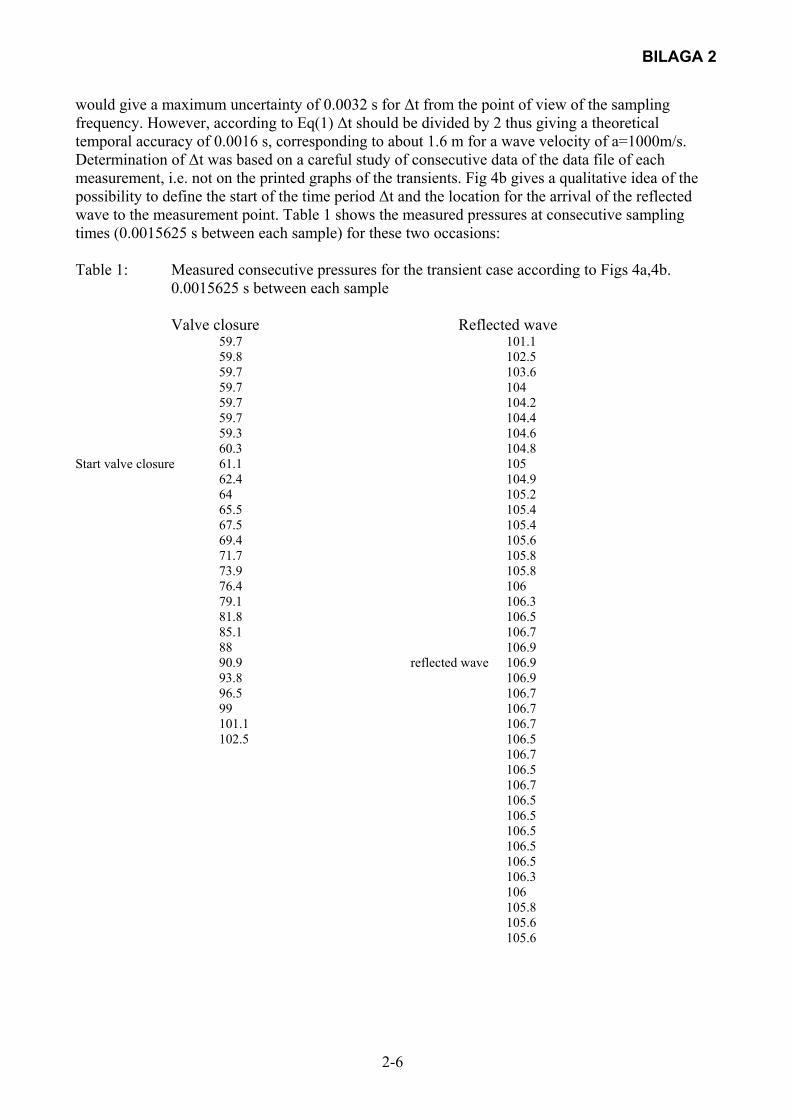
would give a maximum uncertainty of 0.0032 s for ∆t from the point of view of the sampling frequency. However, according to Eq(1) ∆t should be divided by 2 thus giving a theoretical temporal accuracy of 0.0016 s, corresponding to about 1.6 m for a wave velocity of a=1000m/s. Determination of ∆t was based on a careful study of consecutive data of the data file of each measurement, i.e. not on the printed graphs of the transients. Fig 4b gives a qualitative idea of the possibility to define the start of the time period ∆t and the location for the arrival of the reflected wave to the measurement point. Table 1 shows the measured pressures at consecutive sampling times (0.0015625 s between each sample) for these two occasions: Table 1: Measured consecutive pressures for the transient case according to Figs 4a,4b.

0.0015625 s between each sample Valve closure Reflected wave

59.7 101.1 59.8 102.5 59.7 103.6 59.7 104 59.7 104.2 59.7 104.4 59.3 104.6

60.3 104.8 Start valve closure 61.1 105

62.4 104.9 64 105.2 65.5 105.4 67.5 105.4 69.4 105.6 71.7 105.8 73.9 105.8 76.4 106 79.1 106.3 81.8 106.5 85.1 106.7 88 106.9 90.9 reflected wave 106.9 93.8 106.9 96.5 106.7 99 106.7 101.1 106.7 102.5 106.5 106.7 106.5 106.7 106.5 106.5 106.5 106.5 106.5 106.3 106 105.8 105.6 105.6

BILAGA 2

2-7

Table 1, the left hand column, shows the steady state operational pressure at the ball valve amounting to 59.7–59.9 m H 2 O and with the start of the valve closure procedure clearly visible as an accelerated increase of the pressure (60.3, 61.1 m H 2 O etc). In this case the start of the pressure rise would be assumed to be the time corresponding to 61.1 m H 2 O. Table 1, the right hand column, shows the slowly increasing pressure due to the “line-packing” effect. When the pressure has reached 106.9 m H 2 O it starts decreasing again, indicating the arrival of the reflected wave to the pressure measurement point at the ball valve. It is obvious that there is some uncertainty – say one sample time unit – as to the definition of the time of the start of the initial pressure rise. In this specific transient flow case the arrival time of the reflected wave seems to be well-defined. However, in other cases there might be an uncertainty here too. The wave velocity is the second entity, which is required for locating a leak. There are basically two ways of addressing the problem of determining the pressure wave velocity, either using theoretical expressions based on the pipe and liquid properties or deducing the velocity from the measured transient. The theoretical approach is based on the formula (for thin-walled pipes):

p

1v

v

v

EeCED

1

E

a

⋅⋅⋅

+

ρ= (4)

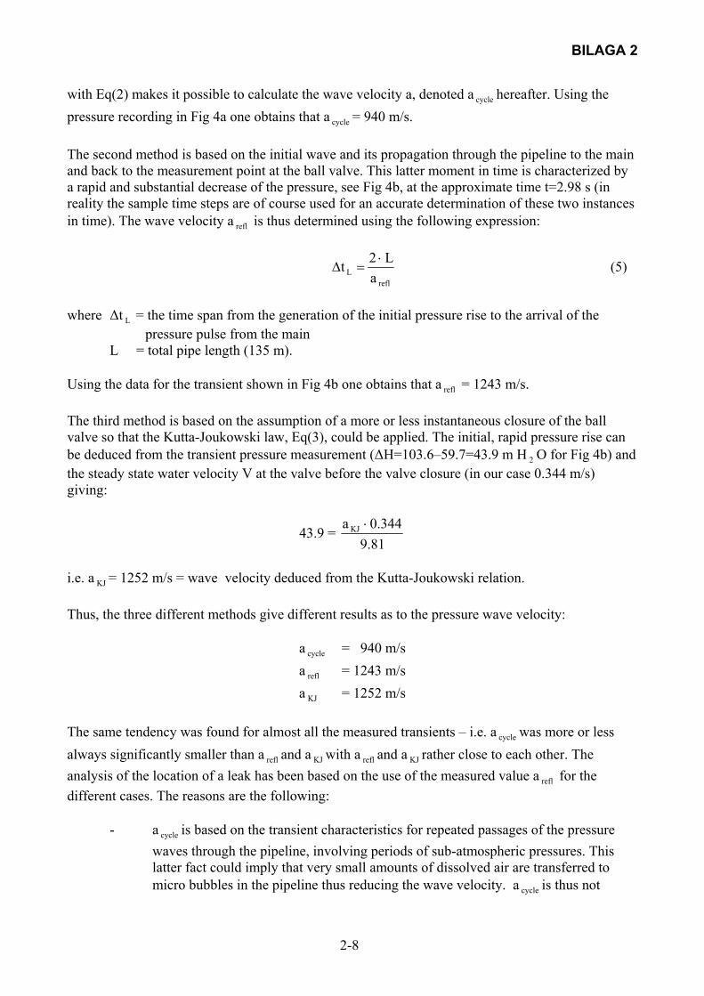
where E v ,E p = elastic modulus for water and pipe material respectively D = pipe inner diameter e = pipe wall thickness C1 = constant of the order of 1 depending on the axial tension properties of the pipeline. Application of Eq(4) does of course require that appropriate knowledge of the pipeline is available. If this is the case one will at least obtain an approximate value of the wave velocity as there might be some uncertainty about some of the variables in Eq(4) and as certain peculiarities of the pipeline, such as the existence of small bubbles in the water or pipe joint effects, might affect the wave velocity. The second approach is based on an analysis of the measured transient and should preferably be used, if possible, as one would expect that the “true” wave velocity should be obtained in this way. The way such an analysis is performed will of course depend on the specific nature of a transient. The following discussion refers to the transients measured at Bulltofta and reference is made to the example shown in Figs 4a,4b. One could thus evaluate the wave velocity according to three methods and they should ideally give the same result. The first method is based on the oscillating nature of the pressure transient after valve closure. The time period T for the oscillating pressure can be determined with a good accuracy provided the pressure recording contains several pressure cycles. Knowledge of the total pipe length L together

BILAGA 2

2-8

with Eq(2) makes it possible to calculate the wave velocity a, denoted a cycle hereafter. Using the pressure recording in Fig 4a one obtains that a cycle = 940 m/s. The second method is based on the initial wave and its propagation through the pipeline to the main and back to the measurement point at the ball valve. This latter moment in time is characterized by a rapid and substantial decrease of the pressure, see Fig 4b, at the approximate time t=2.98 s (in reality the sample time steps are of course used for an accurate determination of these two instances in time). The wave velocity a refl is thus determined using the following expression:

refl

L aL2t ⋅

=∆ (5)

where ∆t L = the time span from the generation of the initial pressure rise to the arrival of the pressure pulse from the main L = total pipe length (135 m). Using the data for the transient shown in Fig 4b one obtains that a refl = 1243 m/s. The third method is based on the assumption of a more or less instantaneous closure of the ball valve so that the Kutta-Joukowski law, Eq(3), could be applied. The initial, rapid pressure rise can be deduced from the transient pressure measurement (∆H=103.6–59.7=43.9 m H 2 O for Fig 4b) and the steady state water velocity V at the valve before the valve closure (in our case 0.344 m/s) giving:

43.9 = 81.9

344.0a KJ ⋅

i.e. a KJ = 1252 m/s = wave velocity deduced from the Kutta-Joukowski relation. Thus, the three different methods give different results as to the pressure wave velocity:

a cycle = 940 m/s a refl = 1243 m/s a KJ = 1252 m/s

The same tendency was found for almost all the measured transients – i.e. a cycle was more or less always significantly smaller than a refl and a KJ with a refl and a KJ rather close to each other. The analysis of the location of a leak has been based on the use of the measured value a refl for the different cases. The reasons are the following:

- a cycle is based on the transient characteristics for repeated passages of the pressure waves through the pipeline, involving periods of sub-atmospheric pressures. This latter fact could imply that very small amounts of dissolved air are transferred to micro bubbles in the pipeline thus reducing the wave velocity. a cycle is thus not

BILAGA 2

2-9

assumed to be representative for the determination of the leak location which only utilizes the initial part of the transient phase without any sub-atmospheric pressures

- a KJ is based on the assumption that the valve closure is instantaneous, i.e. it is finished before the reflected wave from the leak reaches the pressure measurement point. This was, however, more or less true in most of the studied cases. A further uncertainty is related to the determination of the relevant water velocity which is based on the flow meter readings (pipeline and leak respectively) and an accurate measure of the inner diameter of the pipeline

- the theoretical wave velocities computed according to a modified expression of Eq(4) considering the fact that D/e<25 for the experimental set-up are:

41.8 mm pipe: 1357 m/s 53.0 mm pipe: 1359 m/s

- These theoretical calculations assumed that the constant C1 =1.0, E p =210·10 9

N/m 2 and that water and pipe material are perfectly homogeneous. Some aberration might exist in reality causing the real wave velocity to be somewhat smaller. Thus a refl and a KJ are the experimental wave velocities closest to the theoretical ones

- the determination of a refl is based on two parameters which could be measured with good accuracy, i.e. pipe length and time duration.

NUMERICAL SIMULATION OF THE LEAK EFFECT ON A TRANSIENT A computer program was developed in order to try to simulate the transient flow situations measured at the experimental set-up at Bulltofta. The primary goal was to investigate the applicability of a rather straightforward computational description of the interaction between transient pressure waves and a leak. For that purpose the computations were limited to a study of the appearance of the initial pressure pulse with a duration starting at the very rapid closure of the valve and finishing when the initial pressure rise had propagated through the entire pipeline and back to the measurement point. The computer program is based on the one-dimensional, unsteady St. Venant’s equations:

0xQ

gAa

tH 2

=∂∂⋅

⋅+

∂∂ (6a)

0gDA2

QQfxH

tQ

gA1

2 =⋅⋅

+∂∂

+∂∂⋅

⋅ (6b)

where H = H(x,t) = p/γ+z = pressure level Q = Q(x,t) = flow in the pipe A = cross sectional area of the pipe D = pipe diameter a = pressure wave velocity f = frictional coefficient x = axial coordinate t = time

BILAGA 2

2-10

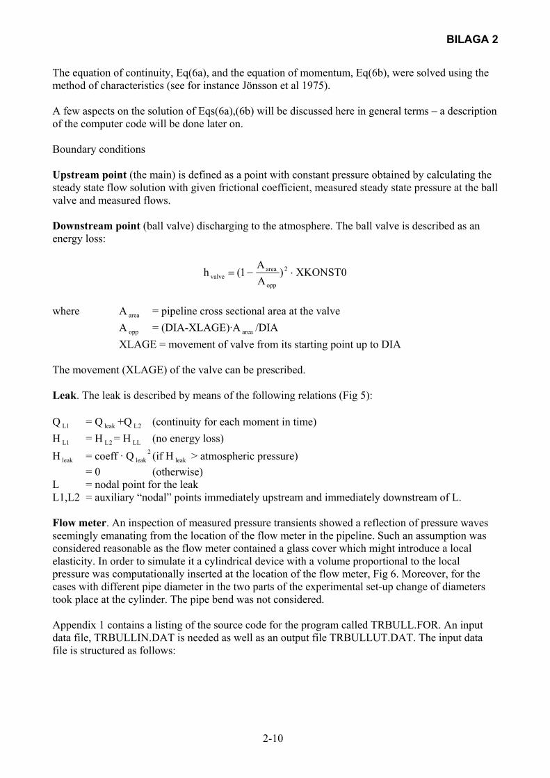
The equation of continuity, Eq(6a), and the equation of momentum, Eq(6b), were solved using the method of characteristics (see for instance Jönsson et al 1975). A few aspects on the solution of Eqs(6a),(6b) will be discussed here in general terms – a description of the computer code will be done later on. Boundary conditions Upstream point (the main) is defined as a point with constant pressure obtained by calculating the steady state flow solution with given frictional coefficient, measured steady state pressure at the ball valve and measured flows. Downstream point (ball valve) discharging to the atmosphere. The ball valve is described as an energy loss:

0XKONST)AA

1(h 2

opp

areavalve ⋅−=

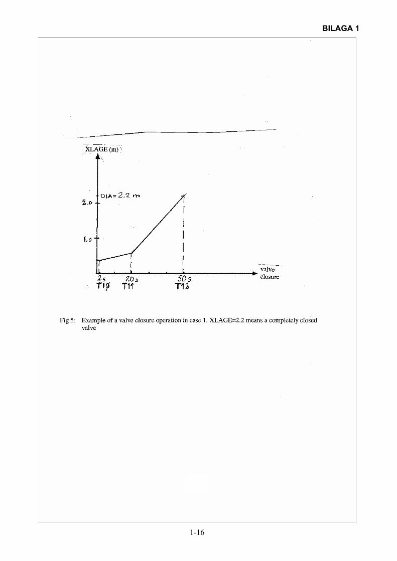
where A area = pipeline cross sectional area at the valve A opp = (DIA-XLAGE)·A area /DIA XLAGE = movement of valve from its starting point up to DIA The movement (XLAGE) of the valve can be prescribed. Leak. The leak is described by means of the following relations (Fig 5): Q 1L = Q leak +Q 2L (continuity for each moment in time) H 1L = H 2L = H LL (no energy loss) H leak = coeff · Q 2

leak (if H leak > atmospheric pressure) = 0 (otherwise) L = nodal point for the leak L1,L2 = auxiliary “nodal” points immediately upstream and immediately downstream of L. Flow meter. An inspection of measured pressure transients showed a reflection of pressure waves seemingly emanating from the location of the flow meter in the pipeline. Such an assumption was considered reasonable as the flow meter contained a glass cover which might introduce a local elasticity. In order to simulate it a cylindrical device with a volume proportional to the local pressure was computationally inserted at the location of the flow meter, Fig 6. Moreover, for the cases with different pipe diameter in the two parts of the experimental set-up change of diameters took place at the cylinder. The pipe bend was not considered. Appendix 1 contains a listing of the source code for the program called TRBULL.FOR. An input data file, TRBULLIN.DAT is needed as well as an output file TRBULLUT.DAT. The input data file is structured as follows:

BILAGA 2

2-11

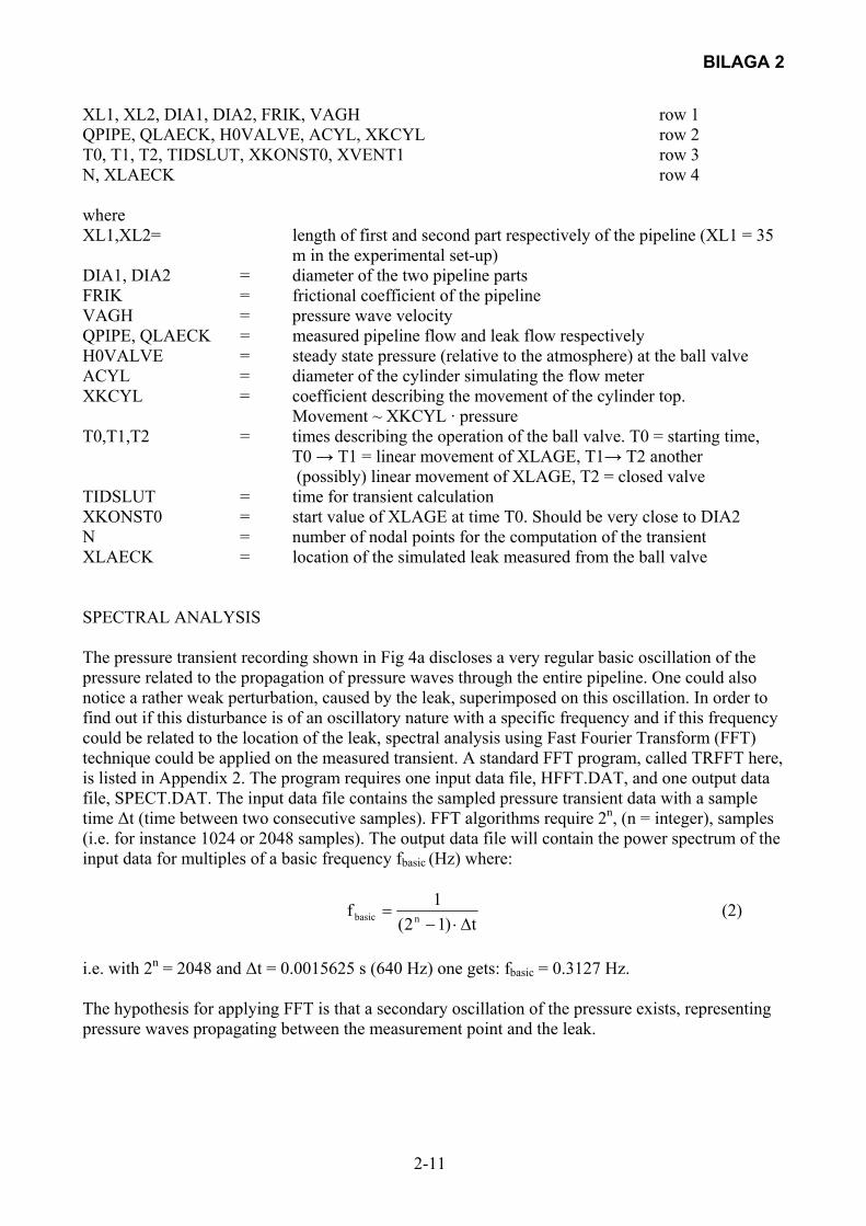
XL1, XL2, DIA1, DIA2, FRIK, VAGH row 1 QPIPE, QLAECK, H0VALVE, ACYL, XKCYL row 2 T0, T1, T2, TIDSLUT, XKONST0, XVENT1 row 3 N, XLAECK row 4 where XL1,XL2= length of first and second part respectively of the pipeline (XL1 = 35

m in the experimental set-up) DIA1, DIA2 = diameter of the two pipeline parts FRIK = frictional coefficient of the pipeline VAGH = pressure wave velocity QPIPE, QLAECK = measured pipeline flow and leak flow respectively H0VALVE = steady state pressure (relative to the atmosphere) at the ball valve ACYL = diameter of the cylinder simulating the flow meter XKCYL = coefficient describing the movement of the cylinder top. Movement ~ XKCYL · pressure T0,T1,T2 = times describing the operation of the ball valve. T0 = starting time,

T0 → T1 = linear movement of XLAGE, T1→ T2 another (possibly) linear movement of XLAGE, T2 = closed valve

TIDSLUT = time for transient calculation XKONST0 = start value of XLAGE at time T0. Should be very close to DIA2 N = number of nodal points for the computation of the transient XLAECK = location of the simulated leak measured from the ball valve SPECTRAL ANALYSIS The pressure transient recording shown in Fig 4a discloses a very regular basic oscillation of the pressure related to the propagation of pressure waves through the entire pipeline. One could also notice a rather weak perturbation, caused by the leak, superimposed on this oscillation. In order to find out if this disturbance is of an oscillatory nature with a specific frequency and if this frequency could be related to the location of the leak, spectral analysis using Fast Fourier Transform (FFT) technique could be applied on the measured transient. A standard FFT program, called TRFFT here, is listed in Appendix 2. The program requires one input data file, HFFT.DAT, and one output data file, SPECT.DAT. The input data file contains the sampled pressure transient data with a sample time ∆t (time between two consecutive samples). FFT algorithms require 2n, (n = integer), samples (i.e. for instance 1024 or 2048 samples). The output data file will contain the power spectrum of the input data for multiples of a basic frequency fbasic (Hz) where:

t)12(

1f nbasic ∆⋅−= (2)

i.e. with 2n = 2048 and ∆t = 0.0015625 s (640 Hz) one gets: fbasic = 0.3127 Hz. The hypothesis for applying FFT is that a secondary oscillation of the pressure exists, representing pressure waves propagating between the measurement point and the leak.

BILAGA 2

2-12

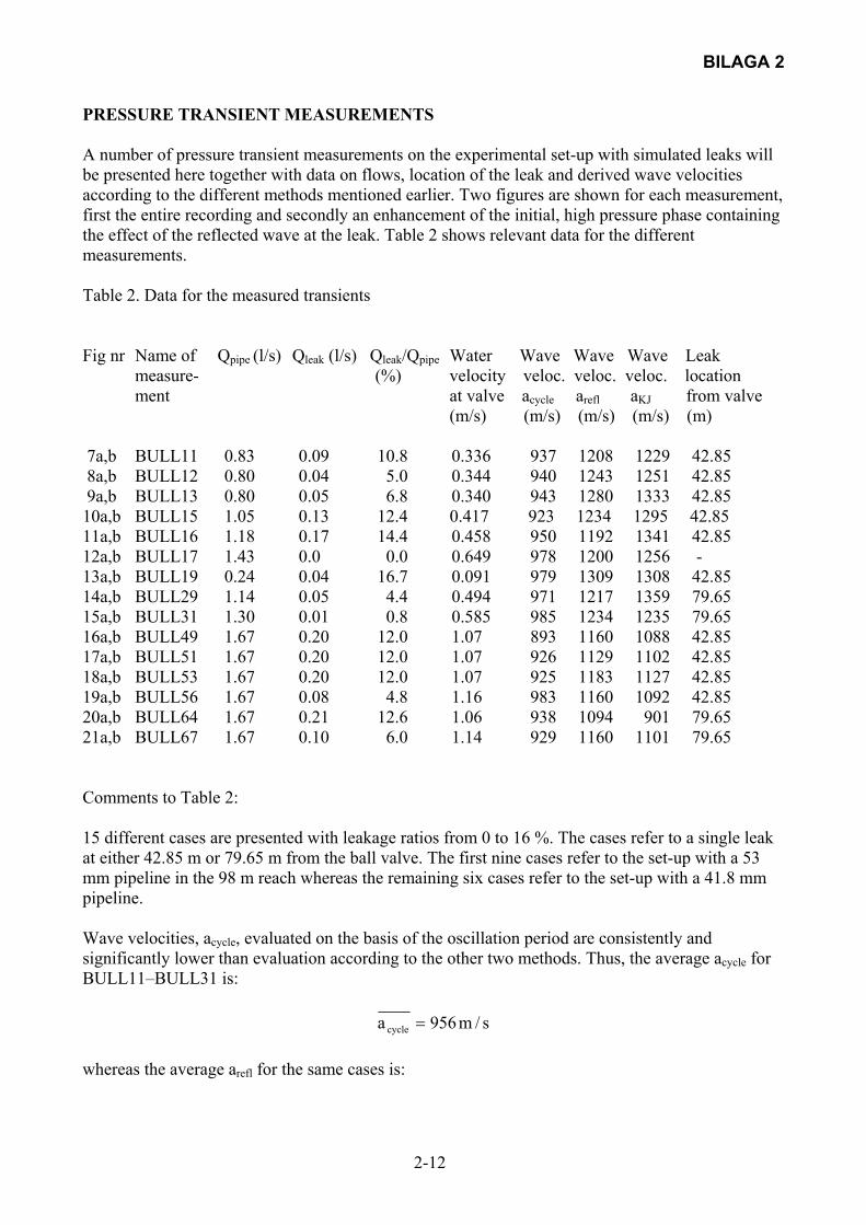
PRESSURE TRANSIENT MEASUREMENTS A number of pressure transient measurements on the experimental set-up with simulated leaks will be presented here together with data on flows, location of the leak and derived wave velocities according to the different methods mentioned earlier. Two figures are shown for each measurement, first the entire recording and secondly an enhancement of the initial, high pressure phase containing the effect of the reflected wave at the leak. Table 2 shows relevant data for the different measurements. Table 2. Data for the measured transients Fig nr Name of Qpipe (l/s) Qleak (l/s) Qleak/Qpipe Water Wave Wave Wave Leak measure- (%) velocity veloc. veloc. veloc. location ment at valve acycle arefl aKJ from valve (m/s) (m/s) (m/s) (m/s) (m) 7a,b BULL11 0.83 0.09 10.8 0.336 937 1208 1229 42.85 8a,b BULL12 0.80 0.04 5.0 0.344 940 1243 1251 42.85 9a,b BULL13 0.80 0.05 6.8 0.340 943 1280 1333 42.85 10a,b BULL15 1.05 0.13 12.4 0.417 923 1234 1295 42.85 11a,b BULL16 1.18 0.17 14.4 0.458 950 1192 1341 42.85 12a,b BULL17 1.43 0.0 0.0 0.649 978 1200 1256 - 13a,b BULL19 0.24 0.04 16.7 0.091 979 1309 1308 42.85 14a,b BULL29 1.14 0.05 4.4 0.494 971 1217 1359 79.65 15a,b BULL31 1.30 0.01 0.8 0.585 985 1234 1235 79.65 16a,b BULL49 1.67 0.20 12.0 1.07 893 1160 1088 42.85 17a,b BULL51 1.67 0.20 12.0 1.07 926 1129 1102 42.85 18a,b BULL53 1.67 0.20 12.0 1.07 925 1183 1127 42.85 19a,b BULL56 1.67 0.08 4.8 1.16 983 1160 1092 42.85 20a,b BULL64 1.67 0.21 12.6 1.06 938 1094 901 79.65 21a,b BULL67 1.67 0.10 6.0 1.14 929 1160 1101 79.65 Comments to Table 2: 15 different cases are presented with leakage ratios from 0 to 16 %. The cases refer to a single leak at either 42.85 m or 79.65 m from the ball valve. The first nine cases refer to the set-up with a 53 mm pipeline in the 98 m reach whereas the remaining six cases refer to the set-up with a 41.8 mm pipeline. Wave velocities, acycle, evaluated on the basis of the oscillation period are consistently and significantly lower than evaluation according to the other two methods. Thus, the average acycle for BULL11–BULL31 is:

s/m956a cycle =

whereas the average arefl for the same cases is:

BILAGA 2

2-13

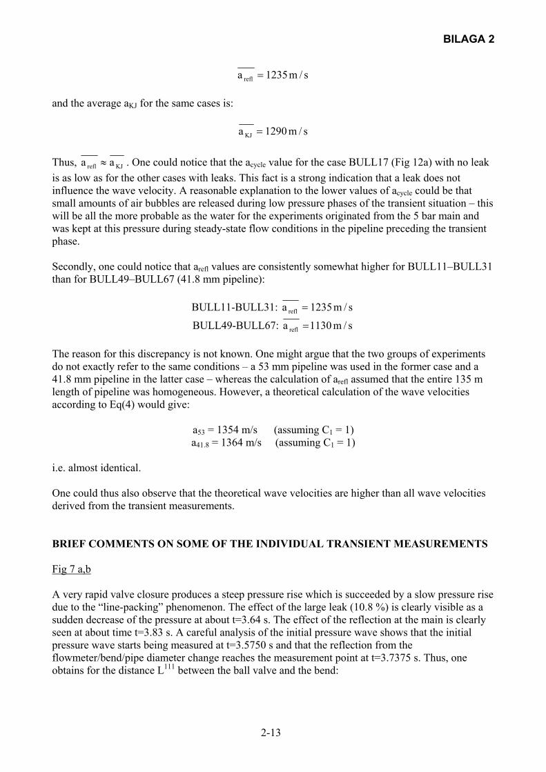
s/m1235a refl =

and the average aKJ for the same cases is:

s/m1290a KJ =

Thus, KJrefl aa ≈ . One could notice that the acycle value for the case BULL17 (Fig 12a) with no leak is as low as for the other cases with leaks. This fact is a strong indication that a leak does not influence the wave velocity. A reasonable explanation to the lower values of acycle could be that small amounts of air bubbles are released during low pressure phases of the transient situation – this will be all the more probable as the water for the experiments originated from the 5 bar main and was kept at this pressure during steady-state flow conditions in the pipeline preceding the transient phase. Secondly, one could notice that arefl values are consistently somewhat higher for BULL11–BULL31 than for BULL49–BULL67 (41.8 mm pipeline):

BULL11-BULL31: s/m1235a refl =

BULL49-BULL67: s/m1130a refl = The reason for this discrepancy is not known. One might argue that the two groups of experiments do not exactly refer to the same conditions – a 53 mm pipeline was used in the former case and a 41.8 mm pipeline in the latter case – whereas the calculation of arefl assumed that the entire 135 m length of pipeline was homogeneous. However, a theoretical calculation of the wave velocities according to Eq(4) would give:

a53 = 1354 m/s (assuming C1 = 1) a41.8 = 1364 m/s (assuming C1 = 1)

i.e. almost identical. One could thus also observe that the theoretical wave velocities are higher than all wave velocities derived from the transient measurements. BRIEF COMMENTS ON SOME OF THE INDIVIDUAL TRANSIENT MEASUREMENTS Fig 7 a,b A very rapid valve closure produces a steep pressure rise which is succeeded by a slow pressure rise due to the “line-packing” phenomenon. The effect of the large leak (10.8 %) is clearly visible as a sudden decrease of the pressure at about t=3.64 s. The effect of the reflection at the main is clearly seen at about time t=3.83 s. A careful analysis of the initial pressure wave shows that the initial pressure wave starts being measured at t=3.5750 s and that the reflection from the flowmeter/bend/pipe diameter change reaches the measurement point at t=3.7375 s. Thus, one obtains for the distance L111 between the ball valve and the bend:

BILAGA 2

2-14

5750.37375.31208

L2 111

−=⋅

L111 = 98.2 m

Fig 8 a,b This case is very similar to the one shown in Fig 7 a,b. The leak is smaller (5 %) here but still distinctly visible at about time t=3.04 s when the pressure starts decreasing. The reflection at the main is seen as a rapid drop of the pressure at about time t=3.2 s. A careful analysis shows that the pressure pulse is initiated at time t=2.98437 s and that the reflection from the bend reaches the measurement point at time t=3.14375 s. Thus, one obtains for the distance L111 (same as for Fig 7a,b):

98437.214375.31243

L2 111

−=⋅

L111 = 99 m.

A certain distortion of the pressure oscillation is visible. The small pressure undulation is apparent as discussed earlier, Fig 4 a,b. Fig 9 a,b A very rapid valve closure produces a steep pressure rise. The effect of the leak (6.8 %) is clearly visible at about time t=3.24 s. A small distortion of the pressure oscillations takes place. Reflection at the main is obvious at about time 3.38 s. A careful analysis shows that the pressure pulse is initiated at time t=3.17031 s and that the reflection from the flow meter/bend/diameter change reaches the measurement point at time t=3.3375 s. Thus, one obtains for the distance L111 (same as for Fig 7 a,b):

17031.33375.31186

L2 111

−=⋅

L111 = 99 m.

which agrees very well with the real conditions. Distinct pressure undulation occurs due to the assumed precursor wave. Fig 10 a,b A very rapid valve closure produces a steep pressure rise. The effect of the large leak is clearly visible at about time t=3.02 s. A significant distortion of the pressure oscillations is visible. The reflection from the main s recorded at about time t=3.17 s. A careful analysis shows that the pressure pulse is initiated at time t=2.95469 s and that the reflection from the flow meter/bend/diameter change reaches the measurement point at time t=3.125 s. Thus, one obtains for the distance L111 (same as for Fig 7 a,b):

BILAGA 2

2-15

95469.2125.31234

L2 111

−=⋅

L111 = 105 m

An obvious pressure undulation occurs due to the assumed precursor wave interaction with the bend Fig 11 a,b A slower valve closure, probably slower than the time for a pressure wave to propagate towards the main and back again, produces a less steep pressure wave. However, the effect of the large leak (14 %) is still distinct at about time t=3.2 s. The distortion of the pressure oscillation is very manifest. Moreover, the oscillations are attenuated faster than for cases with a smaller leak. The reflection from the main is detected at about time t=3.36 s. A careful analysis shows that the pressure pulse is initiated at time t=3.13125 s and that the reflection from the flow meter/bend/diameter change reaches the measurement point at time t=3.2934 s giving for L111 (same definition as for Fig 7 a,b):

13125.329344.31192

L2 111

−=⋅

L111 = 99.7 m.

Distinct pressure undulations occur due to the assumed precursor wave interaction with the bend. Fig 12 a,b No leak. A very rapid valve closure produces a steep pressure pulse. After that the pressure rises slowly due to the “line packing” effect. At about time t=3.22 s the pressure decreases, unknown reason. The reflection at the main is clearly visible at about time t=3.3 s. A careful analysis shows that the pressure pulse is initiated at time t=3.0687 s and that the reflection at the flow meter/bend/diameter change reaches the measurement point at time t=3.231 s giving for L111:

0687.32391.31200

L2 111

−=⋅

L111 = 102.2 m.

The unknown pressure drop at time t=3.2172 s corresponds to a distance LIV using to normal hydraulic transient speed:

0687.32172.31200

L2 IV

−=⋅

LIV = 89 m.

As there is no change in pipeline properties at this location it is concluded that the use of the normal wave speed is not appropriate – instead indicating at the effect of a precursor wave. The pressure oscillations do not show any distortion and the attenuation of the amplitudes is rather low compared to cases with a leak – i.e. more oscillations are visible.

BILAGA 2

2-16

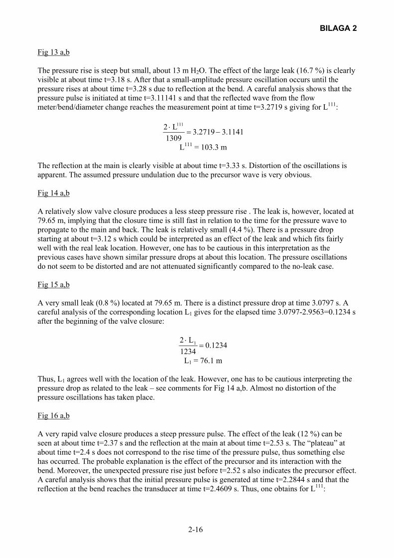
Fig 13 a,b The pressure rise is steep but small, about 13 m H2O. The effect of the large leak (16.7 %) is clearly visible at about time t=3.18 s. After that a small-amplitude pressure oscillation occurs until the pressure rises at about time t=3.28 s due to reflection at the bend. A careful analysis shows that the pressure pulse is initiated at time t=3.11141 s and that the reflected wave from the flow meter/bend/diameter change reaches the measurement point at time t=3.2719 s giving for L111:

1141.32719.31309

L2 111

−=⋅

L111 = 103.3 m The reflection at the main is clearly visible at about time t=3.33 s. Distortion of the oscillations is apparent. The assumed pressure undulation due to the precursor wave is very obvious. Fig 14 a,b A relatively slow valve closure produces a less steep pressure rise . The leak is, however, located at 79.65 m, implying that the closure time is still fast in relation to the time for the pressure wave to propagate to the main and back. The leak is relatively small (4.4 %). There is a pressure drop starting at about t=3.12 s which could be interpreted as an effect of the leak and which fits fairly well with the real leak location. However, one has to be cautious in this interpretation as the previous cases have shown similar pressure drops at about this location. The pressure oscillations do not seem to be distorted and are not attenuated significantly compared to the no-leak case. Fig 15 a,b A very small leak (0.8 %) located at 79.65 m. There is a distinct pressure drop at time 3.0797 s. A careful analysis of the corresponding location L1 gives for the elapsed time 3.0797-2.9563=0.1234 s after the beginning of the valve closure:

1234.01234

L2 1 =⋅

L1 = 76.1 m

Thus, L1 agrees well with the location of the leak. However, one has to be cautious interpreting the pressure drop as related to the leak – see comments for Fig 14 a,b. Almost no distortion of the pressure oscillations has taken place. Fig 16 a,b A very rapid valve closure produces a steep pressure pulse. The effect of the leak (12 %) can be seen at about time t=2.37 s and the reflection at the main at about time t=2.53 s. The “plateau” at about time t=2.4 s does not correspond to the rise time of the pressure pulse, thus something else has occurred. The probable explanation is the effect of the precursor and its interaction with the bend. Moreover, the unexpected pressure rise just before t=2.52 s also indicates the precursor effect. A careful analysis shows that the initial pressure pulse is generated at time t=2.2844 s and that the reflection at the bend reaches the transducer at time t=2.4609 s. Thus, one obtains for L111:

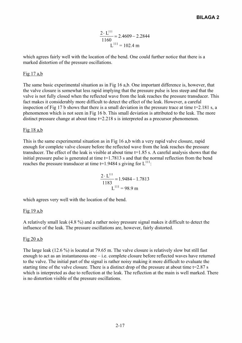
BILAGA 2

2-17

2844.24609.21160

L2 111

−=⋅

L111 = 102.4 m

which agrees fairly well with the location of the bend. One could further notice that there is a marked distortion of the pressure oscillations. Fig 17 a,b The same basic experimental situation as in Fig 16 a,b. One important difference is, however, that the valve closure is somewhat less rapid implying that the pressure pulse is less steep and that the valve is not fully closed when the reflected wave from the leak reaches the pressure transducer. This fact makes it considerably more difficult to detect the effect of the leak. However, a careful inspection of Fig 17 b shows that there is a small deviation in the pressure trace at time t=2.181 s, a phenomenon which is not seen in Fig 16 b. This small deviation is attributed to the leak. The more distinct pressure change at about time t=2.218 s is interpreted as a precursor phenomenon. Fig 18 a,b This is the same experimental situation as in Fig 16 a,b with a very rapid valve closure, rapid enough for complete valve closure before the reflected wave from the leak reaches the pressure transducer. The effect of the leak is visible at about time t=1.85 s. A careful analysis shows that the initial pressure pulse is generated at time t=1.7813 s and that the normal reflection from the bend reaches the pressure transducer at time t=1.9484 s giving for L111:

7813.19484.11183

L2 111

−=⋅

L111 = 98.9 m

which agrees very well with the location of the bend. Fig 19 a,b A relatively small leak (4.8 %) and a rather noisy pressure signal makes it difficult to detect the influence of the leak. The pressure oscillations are, however, fairly distorted. Fig 20 a,b The large leak (12.6 %) is located at 79.65 m. The valve closure is relatively slow but still fast enough to act as an instantaneous one – i.e. complete closure before reflected waves have returned to the valve. The initial part of the signal is rather noisy making it more difficult to evaluate the starting time of the valve closure. There is a distinct drop of the pressure at about time t=2.87 s which is interpreted as due to reflection at the leak. The reflection at the main is well marked. There is no distortion visible of the pressure oscillations.

BILAGA 2

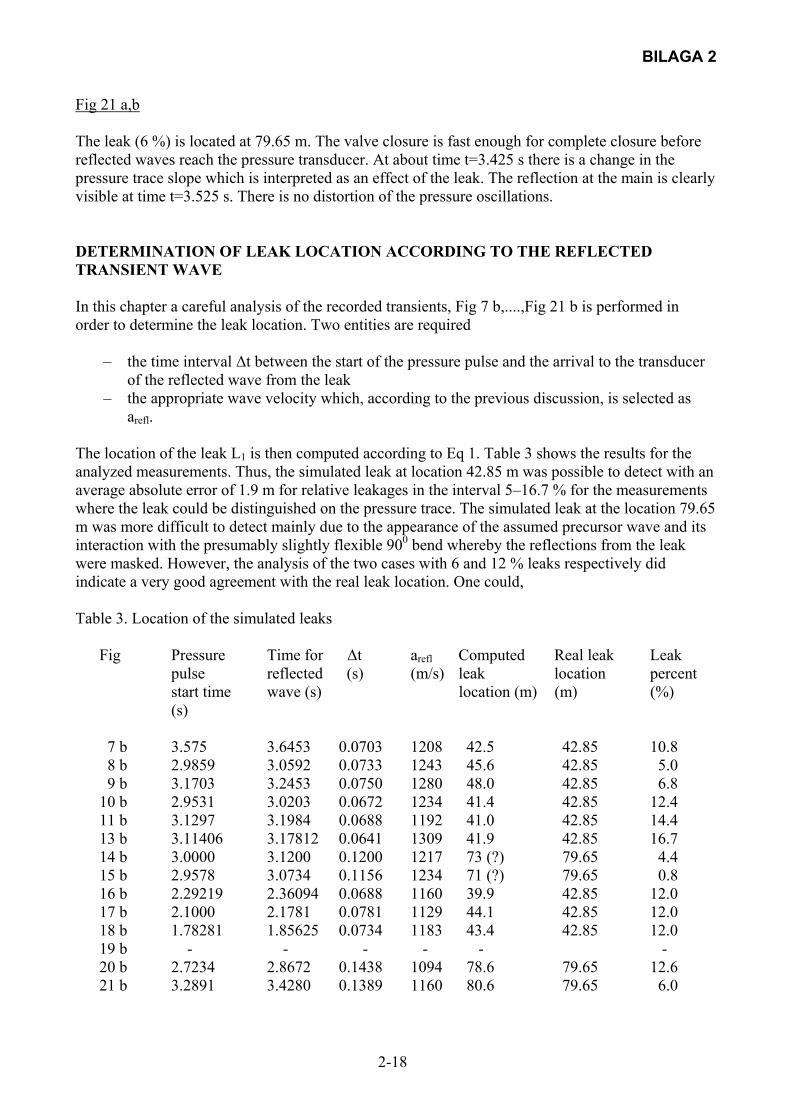
2-18

Fig 21 a,b The leak (6 %) is located at 79.65 m. The valve closure is fast enough for complete closure before reflected waves reach the pressure transducer. At about time t=3.425 s there is a change in the pressure trace slope which is interpreted as an effect of the leak. The reflection at the main is clearly visible at time t=3.525 s. There is no distortion of the pressure oscillations. DETERMINATION OF LEAK LOCATION ACCORDING TO THE REFLECTED TRANSIENT WAVE In this chapter a careful analysis of the recorded transients, Fig 7 b,....,Fig 21 b is performed in order to determine the leak location. Two entities are required

– the time interval ∆t between the start of the pressure pulse and the arrival to the transducer

of the reflected wave from the leak – the appropriate wave velocity which, according to the previous discussion, is selected as

arefl. The location of the leak L1 is then computed according to Eq 1. Table 3 shows the results for the analyzed measurements. Thus, the simulated leak at location 42.85 m was possible to detect with an average absolute error of 1.9 m for relative leakages in the interval 5–16.7 % for the measurements where the leak could be distinguished on the pressure trace. The simulated leak at the location 79.65 m was more difficult to detect mainly due to the appearance of the assumed precursor wave and its interaction with the presumably slightly flexible 900 bend whereby the reflections from the leak were masked. However, the analysis of the two cases with 6 and 12 % leaks respectively did indicate a very good agreement with the real leak location. One could, Table 3. Location of the simulated leaks

Fig Pressure Time for ∆t arefl Computed Real leak Leak pulse reflected (s) (m/s) leak location percent start time wave (s) location (m) (m) (%) (s) 7 b 3.575 3.6453 0.0703 1208 42.5 42.85 10.8 8 b 2.9859 3.0592 0.0733 1243 45.6 42.85 5.0 9 b 3.1703 3.2453 0.0750 1280 48.0 42.85 6.8 10 b 2.9531 3.0203 0.0672 1234 41.4 42.85 12.4 11 b 3.1297 3.1984 0.0688 1192 41.0 42.85 14.4 13 b 3.11406 3.17812 0.0641 1309 41.9 42.85 16.7 14 b 3.0000 3.1200 0.1200 1217 73 (?) 79.65 4.4 15 b 2.9578 3.0734 0.1156 1234 71 (?) 79.65 0.8 16 b 2.29219 2.36094 0.0688 1160 39.9 42.85 12.0 17 b 2.1000 2.1781 0.0781 1129 44.1 42.85 12.0 18 b 1.78281 1.85625 0.0734 1183 43.4 42.85 12.0 19 b - - - - - - 20 b 2.7234 2.8672 0.1438 1094 78.6 79.65 12.6 21 b 3.2891 3.4280 0.1389 1160 80.6 79.65 6.0

BILAGA 2

2-19

however, expect that problems with pressure waves induced by moving bends will not exist in cases with long pipelines either buried in the ground or strongly anchored in other ways, thus making it easier to distinguish a leak from a transient pressure recording. Another general conclusion from the measurements is that it seems to be greatly advantageous if a steep pressure pulse can be generated – i.e. a pressure wave with a rise (or decrease) time which is smaller than the required time for the pulse to propagate to the leak and back to the pressure transducer. A third, and obvious conclusion concerns the necessity to determine the appropriate pressure wave velocity accurately in order to arrive at a fairly good location of the leak. Thus, the experiments indicate that the best approach is to derive (if possible) an appropriate specific velocity from each pressure transient measurement instead of using theoretical expressions for the wave velocity. One should also be aware that there are different ways of deducing experimental wave velocities – the general approach should be a method which as much as possible resembles the situation for leak detection. That statement implies in the cases reported here that the initial part of the pressure recording should be used. NUMERICAL SIMULATION OF THE EFFECT OF A LEAK ON THE TRANSIENT The numerical model described in the chapter on ‘Numerical simulation of the leak effect on a transient’ (see also Appendix 1) was used for calculating the effect of the leak on the transients discussed in the chapter on ‘Pressure transient measurements’. Emphasis was put on an effort to simulate the initial phase of the transient, i.e. the time period from valve closure to the return of the reflected wave from the main. Specifically, the appearance of the reflected wave from the leak is of interest. In each case, the wave velocity arefl , derived from the corresponding transient measurement, has been used implying that the calculated and measured time scales are in full agreement for the return of the pressure pulse from the main. The valve closure operations were not measured in the experiments, thus a rapid, two-step procedure was adopted according to valve loss and input data described in the chapter ‘Numerical simulation of the leak effect on a transient, Boundary conditions’. The time scale for the valve closure was obtained from an inspection of the measured transients. The leak discharge coefficient XKLX in:

H1LX1 = XKLX · Q1L2 (see appendix) where H1LX1 = instantaneous pressure in the pipeline at the leakage point Q1L = instantaneous leak flow was manipulated a bit in order to simulate a possible change of leak area due to varying pressures in the pipeline:

XKLX1 = XKLX0 · HLX10/HLX1

where XKLX0 = discharge coefficient for the leak at steady state HLX10 = steady state pressure at the leakage point. The computed transients are shown as Figs 7c, 8c, ...., 21c. Brief comments to each of the calculations are given below together with the input data file.

BILAGA 2

2-20

Input data file for Fig 7c, Bull 11 34.9 98.35 0.040 0.050 0.040 1208 XL1,XL2,DIA1,DIA2,FRIK,VAGH 0.00083 0.00009 60.0 0.002 0.00005 QPIPE,QLAECK,H0VALVE,ACYL,XKCYL 0.1 0.113 0.15 0.70 100000 0.049 T0,T1,T2,TIDSLUT,XKONST0,XVENT1 1000 42.85 N,XLAECK The initial pressure rise is somewhat higher than for the corresponding measurement due to the fact that the used arefl is higher than the derived acycle – see Table 1. That goes for all the computations and this comment will thus not be repeated for the subsequent cases. After the steep pressure rise the pressure levels off at about 116 m H2O, rising very slowly due to the line-packing effect. At time t=0.1706 s the pressure starts decreasing fairly slowly due to the arrival of the reflected wave from the leak. This is in good agreement with the measured transient, Fig 7b. The computed pressure transient continues to decrease thereafter for a time period equivalent to the valve closure time and then the pressure is more or less constant until the reflected wave from the cylinder (supposedly simulating the flow meter and the pipe diameter change) returns, time t=0.264 s. Reflection from the main is seen at time t=0.323 s. The measured transient, Fig 7b, shows an increased pressure (peak 120 m H2O) at this time and qualitatively the same feature can be seen in the computed one. However, there are some discrepancies between the measured and the computed transients for the interval between the reflection from the leak and the reflection from the main. This is probably due to the effect of the 900 bend (maybe somewhat flexible) and its interaction with a precursor wave and no effort was devoted to such a simulation. This bend effect is common to all measurements but is obviously not seen on the computations. No further reference will be made to this discrepancy. Input data file for Fig 8c, Bull 12 34.9 98.35 0.04 0.05 0.1 1243 XL1,XL2,DIA1,DIA2,FRIK,VAGH 0.0008 0.00004 49.7 0.0020 0.00005 QPIPE,QLAECK,H0VALVE,ACYL,XKCYL 0.1 0.1297 0.135 0.70 100000 0.0499 T0,T1,T2,TIDSLUT,XKONST0,XVENT1 1000 42.85 N,XLAECK The computed transient is similar to the one shown in Fig 7c. The effect of the leak (5 %) is clearly visible at about time t=0.165 s as well as the reflection from the cylinder/pipe diameter change. The effect of the main is seen at time 0.32 s. The agreement with the measured transient, Fig 8b, is fairly good concerning the leak effect and the reflection at the main. Input data file for Fig 9c, Bull 13 34.9 98.35 0.04 0.05 0.1 1280 XL1,XL2,DIA1,DIA2,FRIK,VAGH 0.0008 0.00005 49.9 0.0020 0.00005 QPIPE,QLAECK,H0VALVE,ACYL,XKCYL0.1 0.1250 0.13 0.70 100000 0.0499 T0,T1,T2,TIDSLUT,XKONST0,XVENT1 1000 42.85 N, XLAECK The computed transient is similar to the one in Fig 7c. The leak is clearly visible at about time t=0.165 s as well as the reflection from the cylinder/pipe diameter change. Good agreement with the measured transient, Fig 9b, concerning the effect of the leak and the main.

BILAGA 2

2-21

Input data file for Fig 10c, Bull 15 34.9 98.35 0.04 0.05 0.1 1234 XL1,XL2,DIA1,DIA2,FRIK,VAGH 0.00105 0.00013 48.4 0.0020 0.00005 QPIPE,QLAECK,H0VALVE,ACYL,XKCYL 0.01 0.036 0.04 0.70 100000 0.0499 T0,T1,T2,TIDSLUT,XKONST0,XVENT1 1000 42.85 N,XLAECK The effect of the leak (12.4 %) is very visible at about time t=0.08 s. The subsequent gradual decrease of the pressure is also very distinct and fairly steep. Reflection from the cylinder/pipe diameter change at about time t=0.17 s is also evident. The effect of the leak is well reproduced (compare with Fig 10b) and the same goes for the main. Input data file for Fig 11c, Bull 16 34.9 98.35 0.04 0.05 0.1 1217 XL1,XL2,DIA1,DIA2,FRIK,VAGH 0.00118 0.00017 47.2 0.0020 0.00005 QPIPE,QLAECK,H0VALVE,ACYL,XKCYL 0.1 0.1192 0.13 0.70 100000 0.0499 T0,T1,T2,TIDSLUT,XKONST0,XVENT1 1000 42.85 N,XLAECK The large leak (14.4 %) is very distinct at about time t=0.17 s as well as the reflection at the cylinder/pipe diameter change (time about t=0.26 s) and the reflection at the main (time about t=0.32 s). One has to observe that the computed transient used a faster valve closure than the measured one, Fig 11b, thus causing a difference in pulse steepness. Input data file for Fig 12c, Bull 17 34.9 98.35 0.04 0.05 0.1 1200 XL1,XL2,DIA1,DIA2,FRIK,VAGH 0.00143 0.000000013 45.9 0.0020 0.00005 QPIPE,QLAECK,H0VALVE,ACYL,XKCYL 0.1 0.15 0.155 0.70 100000 0.0499 T0,T1,T2,TIDSLUT,XKONST0,XVENT1 1000 42.85 N,XLAECK Input data file for Fig 12d, Bull 17 34.9 98.35 0.04 0.05 0.1 1200 XL1,XL2,DIA1,DIA2,FRIK,VAGH 0.00143 0.000000013 45.9 0.0020 0.00010 QPIPE,QLAECK,H0VALVE,ACYL,XKCYL 0.1 0.15 0.155 0.70 100000 0.0499 T0,T1,T2,TIDSLUT,XKONST0,XVENT1 1000 42.85 N,XLAECK Input data file for Fig 12e, Bull 17 34.9 98.35 0.04 0.05 0.1 1200 XL1,XL2,DIA1,DIA2,FRIK,VAGH 0.00143 0.000000013 45.9 0.0020 0.00020 QPIPE,QLAECK,H0VALVE,ACYL,XKCYL 0.1 0.15 0.155 0.70 100000 0.0499 T0,T1,T2,TIDSLUT,XKONST0,XVENT1 1000 42.85 N,XLAECK Three different computations are shown in Figs12c,d,e not varying the input data parameters except the elasticity XKCYL for the cylinder. Thus, the XKCYL interval 0.00005–0.002 will affect the reflected wave from the cylinder significantly. The line-packing effect is obvious – i.e. a slow pressure rise in the approximate time interval t=0.15–0.26 s. The effect of the main is seen at about

BILAGA 2

2-22

time t=0.34 s with an increased level of the pressure. The agreement with the measured transient, Fig 12b, is good. Input data file for Fig 13c, Bull 19 34.9 98.35 0.04 0.05 0.1 1309 XL1,XL2,DIA1,DIA2,FRIK,VAGH 0.00024 0.00004 50.1 0.0020 0.00005 QPIPE,QLAECK,H0VALVE,ACYL,XKCYL 0.1 0.1250 0.13 0.70 100000 0.0499 T0,T1,T2,TIDSLUT,XKONST0,XVENT1 1000 42.85 N,XLAECK A large leak (16.7 %). The effect of it is, however, not very evident at about time t=0.165 s due to the low-amplitude, initial pressure pulse. The effect of the cylinder is obvious as well as the effect of the main. The agreement with the measured transient, Fig 13b, is fairly good. Input data file for Fig 14c, Bull 29 34.9 98.35 0.04 0.05 0.1 1217 XL1,XL2,DIA1,DIA2,FRIK,VAGH 0.00114 0.00005 46.1 0.0020 0.00005 QPIPE,QLAECK,H0VALVE,ACYL,XKCYL 0.1 0.1250 0.13 0.70 100000 0.0499 T0,T1,T2,TIDSLUT,XKONST0,XVENT1 1000 79.65 N,XLAECK The small leak (4.4 %) located at 79.65 m is obvious at about time t=0.235 s as well as the effect of the cylinder and the main. It is difficult to see the leak in the measured transient, Fig 14b, due to the possible effect of the precursor wave and the bend. Otherwise the agreement is fairly good. Input data file for Fig 15c, Bull 31 34.9 98.35 0.04 0.05 0.1 1234 XL1,XL2,DIA1,DIA2,FRIK,VAGH 0.00130 0.00001 47.5 0.0020 0.00005 QPIPE,QLAECK,H0VALVE,ACYL,XKCYL 0.1 0.13 0.1484 0.70 100000 0.0499 T0,T1,T2,TIDSLUT,XKONST0,XVENT1 1000 79.65 N,XLAECK The effect of the very small leak (0.8 %) is not distinguishable. Input data file for Fig 18c, Bull 53 34.9 98.35 0.040 0.040 0.100 1183 XL1,XL2,DIA1,DIA2,FRIK,VAGH 0.00167 0.00020 48.5 0.003 0.00005 QPIPE,QLAECK,H0VALVE,ACYL,XKCYL 0.1 0.13 0.15 0.70 100000 0.039 T0,T1,T2,TIDSLUT,XKONST0,XVENT1 1000 42.85 N,XLAECK Input data file for Fig 18d, Bull 53 34.9 98.35 0.040 0.040 0.100 1183 XL1,XL2,DIA1,DIA2,FRIK,VAGH 0.00167 0.00020 48.5 0.003 0.00005 QPIPE,QLAECK,H0VALVE,ACYL,XKCYL 0.1 0.15 0.18 0.70 100000 0.039 T0,T1,T2,TIDSLUT,XKONST0,XVENT1 1000 42.85 N,XLAECK In Figs 18c,d the same pipeline diameter has been used throughout the whole pipeline. Figs 18c,d illustrate the influence of valve closure time on the possibility of detecting the leak (12 %). In Fig

BILAGA 2

2-23

18c the closure time is shorter than the time for the propagation of the wave to the leak and back to the valve (transducer location in the experiments). One can clearly distinguish the slow pressure rise due to the line-packing effect before the reflection from the leak abruptly starts decreasing the pressure at about time t=0.18 s. In Fig 18d the valve is closed after wave reflection from the leak has reached the valve and it is not possible to detect any specific trace of the leak. The effect of the main is clearly seen in both cases at about time t=0.35 s. The reflection from the cylinder occurs at about time t=0.265 s whereas the increased pressure, which is seen in the corresponding measurement in conjunction with the main (Fig 18b, time about t=2.1 s), is not represented. This latter fact is most probably due to the flexible bend effect not represented in the computations. Input data file for Fig 19c, Bull 56 34.9 98.35 0.040 0.040 0.1 1160 XL1,XL2,DIA1,DIA2,FRIK,VAGH 0.00167 0.00008 49.0 0.002 0.00005 QPIPE,QLAECK,H0VALVE,ACYL,XKCYL 0.1 0.125 0.155 0.70 100000 0.039 T0,T1,T2,TIDSLUT,XKONST0,XVENT1 1000 42.85 N,XLAECK The effect of the rather small leak (4.8 %) is seen at about time t=0.17 s after the slow pressure rise due to the line-packing effect. The effect of the main is seen at about time t=0.33 s and the effect of the cylinder at about time t=0.265 s. The pressure rise obtained in the measurement close to the effect of the main is not represented in the computation for the same reason as mentioned in relation to Figs 18c,d. Input data file for Fig 20c, Bull 64 34.9 98.35 0.040 0.040 0.040 1094 XL1,XL2,DIA1,DIA2,FRIK,VAGH 0.00167 0.00021 37.0 0.002 0.00005 QPIPE,QLAECK,H0VALVE,ACYL,XKCYL 0.1 0.15 0.21 0.70 100000 0.039 T0,T1,T2,TIDSLUT,XKONST0,XVENT1 1000 79.65 N,XLAECK The effect of the relatively large leak (12.6 %) at 79.65 m is clearly visible at about time t=0.245 s, whereas the main is barely visible at about time t=0.33 s. There is no pressure rise at all in the pressure trace interval preceding and including the reflection from the main as compared to Fig 20b. Input data file for Fig 21c, Bull 67 34.9 98.35 0.040 0.040 0.1 1160 XL1,XL2,DIA1,DIA2,FRIK,VAGH 0.00167 0.00010 49.0 0.002 0.00005 QPIPE,QLAECK,H0VALVE,ACYL,XKCYL 0.1 0.125 0.155 0.70 100000 0.039 T0,T1,T2,TIDSLUT,XKONST0,XVENT1 1000 79.65 N,XLAECK The effect of the leak (6 %) at location 79.65 m is seen clearly at about time t=0.235 s. The reflection from the main is seen at about time t=0.335 s. There is no maximum pressure peak in the pressure trace interval preceding and including the reflection from the main.

BILAGA 2

2-24

Some general conclusions could be drawn of the transient computations in the pipeline with simulated leaks and comparisons with measurements:

- all computations have clearly shown the influence of a leak on the pressure transient trace after rapid valve closure. If this closure is sufficiently rapid the very steep pressure rise is followed by a more slow pressure rise due to the line-packing effect. The return of the reflected wave from the leak is manifested as an abrupt change of the slope of the pressure trace – i.e. the pressure starts decreasing. The rate of decrease is related to the valve closure characteristics – the faster the closure the faster the decrease. The amount of pressure decrease is related to the initial pressure pulse height and the relative leak rate

- the measured transients show a qualitatively similar behaviour as the computed ones, at least up to the time immediately after the return of the reflected wave from the leak. This was especially evident for the leak at 42.35 m and for leaks larger than 4–5 %. This fact is an indication that the description of the leak in the computations is acceptable

- the computations do also show that a slow valve closure – i.e. closure time larger than the wave propagation time from the valve to the leak and back – makes it much more difficult to distinguish the effect of the leak

- the leak at 79.65 m was easily distinguishable in the computations. However, it seems as if the leak was masked in most cases in the measurements due to the effect of a precursor wave and a flexible 900 bend. Thus, it would be valuable to perform further and similar measurements on a straight pipeline

- the effect of trying to simulate the possible effect of the flow meter/pipe diameter change/bend by means of a virtual elastic cylinder was not very successful. This approach did, however, qualitatively simulate the pressure rise in the time domain area corresponding to the reflection at the main for the cases with the 40 mm pipeline followed by the 50 mm pipeline (up to Bull31). The cylinder did not represent the pressure development in the same time domain area for the cases with the constant pipe diameter (40 mm) throughout the whole set-up. A few facts could be put forward as indicators of the effect of a precursor wave – i.e. a wave in the pipe material itself interacting with a flexible 900 bend – in the measurements. In the first place a deviation from the expected pressure pulse behaviour (the undulation which occurs shortly after the reflected wave at the 42.85 m leak) begins too soon to be explained by the normal pressure wave velocity and some kind of interaction with the flow meter/pipe diameter change/bend at 98.35 m. Secondly, measurements on transients in a pipeline with a locally flexible bend reported in the literature (Wood et al 1971) disclose an undulating pressure superimposed on the expected flat pressure pulse similar to those obtained in the transient leak measurements.

SPECTRAL ANALYSIS OF TRANSIENTS Two exercises were performed in order to check the potential of spectral analysis of a transient pressure for disclosing the existence of a leak. In the first place a theoretical calculation was carried out on a simple pipeline with a simulated leak as to the transient at pump stop. The empirical transient was then analyzed using an FFT program (Appendix ??). Secondly, FFT analysis was applied to some of the pressure transient measurements on the experimental set-up discussed in this report.

BILAGA 2

2-25

FFT ANALYSIS ON COMPUTED HYDRAULIC TRANSIENTS The theoretical calculations were performed on the simple pipeline, Fig 22. Two reservoirs are connected with a horizontal pipeline, length L, which is equipped with a pump and a shut-off valve. A leak is located at the distance L1. A calculation of the transient pressure at the valve at pump stop and no leak is shown in Fig 23. The relevant input data was as follows: Length of pipeline 1,000 m Static height difference 20 m Frictional coefficient 0.02 Pipe diameter 0.1 m Wave velocity 1,000 m/s Pump head 30 m Steady state flow 0.008 m3/s Start valve closure at time t=1.0 s End valve closure at time t=22.5 s Pump stop at time t=5.5 s Total calculation time t=70 s The time step ∆t=0.02 s was used for the transient calculations which implies that 3,500 data points of the transient pressure at the valve were obtained. Fig 24 shows the computed spectra for two different data sets, each comprising 2,048 points: Fig 24, top: Data points 1,100–3,148 Fig 24, bottom: Data points 1,400–3,448 The basic frequency of the spectra f1 (horizontal axis) is:

Hz0244.002.02048

1f1 =⋅

=

The frequency of the pressure oscillations in Fig 23 is, according to Eq(2):

Hz25.0000,14

000,1f0 =⋅

=

Thus, one should obtain a peak in the spectra at the multiple 24.100244.0

25.0n == which agrees with

the first peak in the spectra. There is also a second peak at about multiple 31 which corresponds to the third harmonic of the basic oscillatory frequency f0 - i.e. f0 is not exactly sinusoidal. Fig 25 shows the calculated transient for the same pipeline but with a leak. Valve closure starts at time t=1.0 s and ends at time t=15.1 s. Pump stop at time t=8.5 s. The steady state leak flow is 0.00051 m3 /s at the location L1 =380 m, i.e. a relative leakage of 6.4 %, otherwise the same input data as for the previous calculation. The basic frequency is still f1 =0.0244 Hz and the basic frequency of the pressure oscillations is still f0 =0.25 Hz. If the leak would produce a superimposed pressure oscillation due to pressure waves propagating between the valve and the leak, its frequency

BILAGA 2

2-26

would be: f01

= Hz66.03804000,1

=⋅

. Fig 26 shows the computed spectra for two different data sets,

each comprising 2,048 data points: Fig 26, top: Data points 1,000–3,048 Fig 26, bottom: Data points 2,400–4,448. Both spectra in Fig 26 show the peaks corresponding to f0 and to its third harmonic in agreement with the no-leak case, Fig 24. There is no sign of any other peak – for instance at multiple n =

0244.066.0 = 27 (f0

1). One could notice, Fig 25, that the leak causes the basic pressure oscillations to

“break down” producing a higher frequency oscillation which, according to Fig 26 bottom, corresponds to the third harmonic of f0. FFT ANALYSIS ON MEASURED TRANSIENTS Some of the measured transients were analyzed as to the spectral contents in the same way as described for the computed ones. Each of the transient recordings (i.e. the full trace) consisted of 6,400 data points (samples) with a time interval of ∆t=0.0015625 s between each point. Fig 27 shows the spectrum for the transient in Fig 7a (Bull 11) for a data set of 2.048 data points from nr

2,700 to nr 4747. The basic frequency f1= 3125.00015625.0048,2

1=

⋅ Hz. The basic frequency of

the oscillating pressure in the whole experimental pipeline set-up is f0=1.735 Hz corresponding to a

peak location of 11 f55.5f3125.0735.1

⋅=⋅ in accordance with Fig 27. There is also a peak at about 19·f1,

corresponding to the third harmonic. There is no further peak in the spectrum which could be attributed to the leak. Fig 28 shows the spectrum for the transient in Fig 11a (Bull 16) for a data set of 2,048 data points starting from nr 2,400. f1 is the same as previously. The basic frequency of the oscillatory pressure is f0=1.759 Hz which implies a peak location at 5.63· f1 which agrees with Fig 28. The third harmonic is also evident but there is no further peak corresponding to the leak. There is no further peak in the spectrum. Fig 29 shows the spectrum for the transient in Fig 14a (Bull 29) for a data set of 2,048 data points starting at nr 2,200. f1 is the same as previously. f0=1.798 Hz implying a peak location at 5.75· f1 which agrees with Fig 29. There is no peak in the spectrum which could be attributed to the leak. Fig 30 shows the spectrum for the transient in Fig 15a (Bull 31) for a data set of 2,048 data points starting at nr 2,100. f1 is the same as previously. The basic frequency of the oscillating pressure in the whole pipeline is f0=1.824 Hz which implies a peak location at 5.84· f1 which is in agreement with Fig 30. As the leak is very small (0.8 %) one could safely assume that the other peaks are higher harmonics of f0. The analysis of the above-mentioned theoretical and experimental hydraulic transients with simulated leaks does not show any extra peaks in the spectra, which could be attributed to the leak. Thus, no evidence has been found that spectral analysis should have the potential of adding any information on leaks in a pipeline.

BILAGA 2

2-27

CONCLUSIONS A number of hydraulic transients, measured on an experimental 135 m long pipeline set-up, have been analyzed as to the influence of a simulated leak on the appearance of the transient. The transients were generated through more or less rapid valve closure at the downstream end of the pipeline. Leaks were simulated at two positions, either 42.85 m or 79.65 m upstream the valve. Relative leak rates up to 16 % of the steady state pipe flow were investigated. A careful analysis of the measured transients were performed in order to determine the location of the leak on the basis of the temporal location of the small reflection of the pressure wave from the leak and the pressure wave velocity. Moreover, numerical simulations of the initial hydraulic transients were carried out in order to theoretically determine the effect of a leak. Finally, determination of the power spectrum of computed and measured hydraulic transients were performed in order to try to distinguish the effect of a leak on the spectrum. Conclusions from the study: Analysis of the measurements:

- The simulated leak at location 42.85 m was possible to detect with an average absolute error of 1.9 m for relative leakages in the interval 5–16.7 % for the measurements where the leak could be distinguished on the pressure trace.

- The simulated leak at the location 79.65 m was more difficult to detect mainly due to the appearance of an assumed precursor wave and its interaction with the presumably slightly flexible 900 bend whereby the reflections from the leak were masked. However, the analysis of the two cases with 6 and 12 % leaks respectively did indicate a very good agreement with the real leak location. However, one could expect that problems with pressure waves induced by moving bends will not exist in cases with long pipelines either buried in the ground or strongly anchored in other ways, thus making it easier to distinguish a leak from a transient pressure recording.

- It seems to be greatly advantageous if a steep pressure pulse can be generated – i.e. a pressure wave with a rise (or decrease) time which is smaller than the required time for the pulse to propagate to the leak and back to the pressure transducer

- A fairly good determination of the location of the leak requires the knowledge of the appropriate pressure wave velocity accurately. The analysis of the experiments indicates that the best approach is to derive (if possible) an appropriate specific velocity from each pressure transient measurement instead of using theoretical expressions for the wave velocity. One should also be aware that there are different ways of deducing experimental wave velocities – the general approach should be a method which as much as possible resembles the situation for leak detection. That statement implies in the cases reported here that the initial part of the pressure recording should be used. Thus, the pressure wave velocity, based on the propagation time for initial pressure wave to travel from the valve to the main and back to the measurement point, was used. Pressure wave velocities were also estimated from the initial steep pressure rise using the Kutta-Joukowski expression and assuming a very rapid (instantaneous) valve closure. In many cases these wave velocities did agree very well with the reflection time wave velocity as described above. However, there is of course always an uncertainty of the real valve closure rapidness and the line-packing effect. Pressure wave velocities, based on the time scale of the oscillating pressures after valve closure, were considerably lower (of the order of 20–30 %) and were not found to be representative for the leak location. The reason for this large discrepancy was not studied further. It does not, however, seem to depend on the leak as the no-leak case showed the same discrepancy. One possible

BILAGA 2

2-28

explanation is that the propagation of the strong pressure drop did release some minute amounts of dissolved gas in the water in the pipeline which would tend to diminish the wave velocity, an effect which would be especially emphasized when deducing the wave velocity from the repeated passage of the pressure waves through the pipeline. In real cases with less pressure drops and less inelastic pipelines this effect would probably not be of any significance.

Analysis of numerical calculations:

- All computations have clearly shown the influence of a leak on the pressure transient trace after rapid valve closure. If this closure is sufficiently rapid the very steep pressure rise is followed by a more slow pressure rise due to the line-packing effect. The return of the reflected wave from the leak is manifested as an abrupt change of the slope of the pressure trace – i.e. the pressure starts decreasing. The rate of decrease is related to the valve closure characteristics – the faster the closure the faster the decrease. The amount of pressure decrease is related to the initial pressure pulse height and the relative leak rate

- The measured transients show a qualitatively similar behaviour as the computed ones, at least up to the time immediately after the return of the reflected wave from the leak. This was especially evident for the leak at 42.35 m and for leaks larger than 4–5 %. This fact is an indication that the description of the leak in the computations is acceptable

- The computations do also show that a slow valve closure – i.e. closure time larger than the wave propagation time from the valve to the leak and back – makes it much more difficult to distinguish the effect of the leak

- The leak at 79.65 m was easily distinguishable in the computations. However, it seems as if the leak was masked in most cases in the measurements due to the effect of a precursor wave and a flexible 900 bend. Thus, it would be valuable to perform further and similar measurements on a straight pipeline

- The effect of trying to simulate the possible effect of the flow meter/pipe diameter change/bend by means of a virtual elastic cylinder was not very successful. This approach did, however, qualitatively simulate the pressure rise in the time domain area corresponding to the reflection at the main for the cases with the 40 mm pipeline followed by the 50 mm pipeline (up to Bull31). The cylinder did not represent the pressure development in the same time domain area for the cases with the constant pipe diameter (40 mm) throughout the whole set-up. A few facts could be put forward as indicators of the effect of a precursor wave – i.e. a wave in the pipe material itself interacting with a flexible 900 bend – in the measurements. In the first place a deviation from the expected pressure pulse behaviour (the undulation which occurs shortly after the reflected wave at the 42.85 m leak) begins too soon to be explained by the normal pressure wave velocity and some kind of interaction with the flow meter/pipe diameter change/bend at 98.35 m. Secondly, measurements on transients in a pipeline with a locally flexible bend reported in the literature disclose an undulating pressure superimposed on the expected flat pressure pulse similar to those obtained in the transient leak measurements.

-

BILAGA 2

2-29

Power spectrum analysis:

- The FFT analysis of theoretical and experimental hydraulic transients with simulated leaks does not show any extra peaks in the spectra which could be attributed to the leak. Thus, no evidence has been found that spectral analysis should have the potential of adding any information on leaks in a pipeline.

REFERENCES Jönsson, L, Larsen, P. 1975:”Kompendium i instationär strömning”. Dep of Water Resources Engineering, Univ of Lund, Sweden Jönsson, L., Svensson, A. 1997:”Läcksökning med hjälp av tryckslagsmätningar – transientmetoden”. VA-Forsk Rapport 1997.10 Wood, J., Chao, S.H. 1971:”Effect of pipeline junctions on waterhammer surges”, ASCE, Transportation Engineering Journal, Aug 1971, pp 441–456

BILAGA 2

2-30

Fig 1. Pipeline between two reservoirs and equipped with a pump and a check valve as a basis for a general discussion on the effect of a leak at a distance L1 on the transient at pump stop

Fig 2. Characteristic appearance of a hydraulic transient at pump stop measured

immediately downstream of the check valve (top figure). Notice the small pressure increase after time ∆t due to a reflected wave from the leak (bottom figure)

BILAGA 2

2-31

Fig 3. Sketch of the experimental set-up for the measurement of hydraulic transients at the

closure of the downstream ball valve. The upstream part of the conduit is attached to a large main and the downstream part is discharging to the atmosphere. Three simulated leak points exist on the conduit. The details of one of these leak points are also shown in the figure

BILAGA 2

2-32

Fig 4a. Example of a measurement of the hydraulic transient at rapid valve closure as a basis

for a discussion of the characteristics of the transient. Qpipe = 0.80 l/s, Qleak = 0.04 l/s. Simulated leak at 42.85 m. Complete pressure trace.

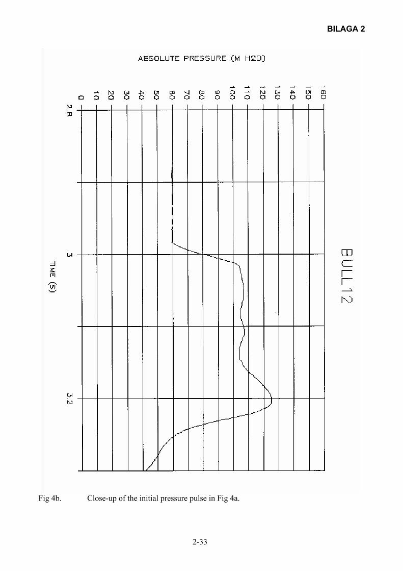
BILAGA 2

2-33

Fig 4b. Close-up of the initial pressure pulse in Fig 4a.

BILAGA 2

2-34

Fig 5. Annotations for the leak description in the computer program

Fig 6. Local elasticity device at the location of the flowmeter. Cylinder with a moving top.

Movement proportional to the pressure at this location

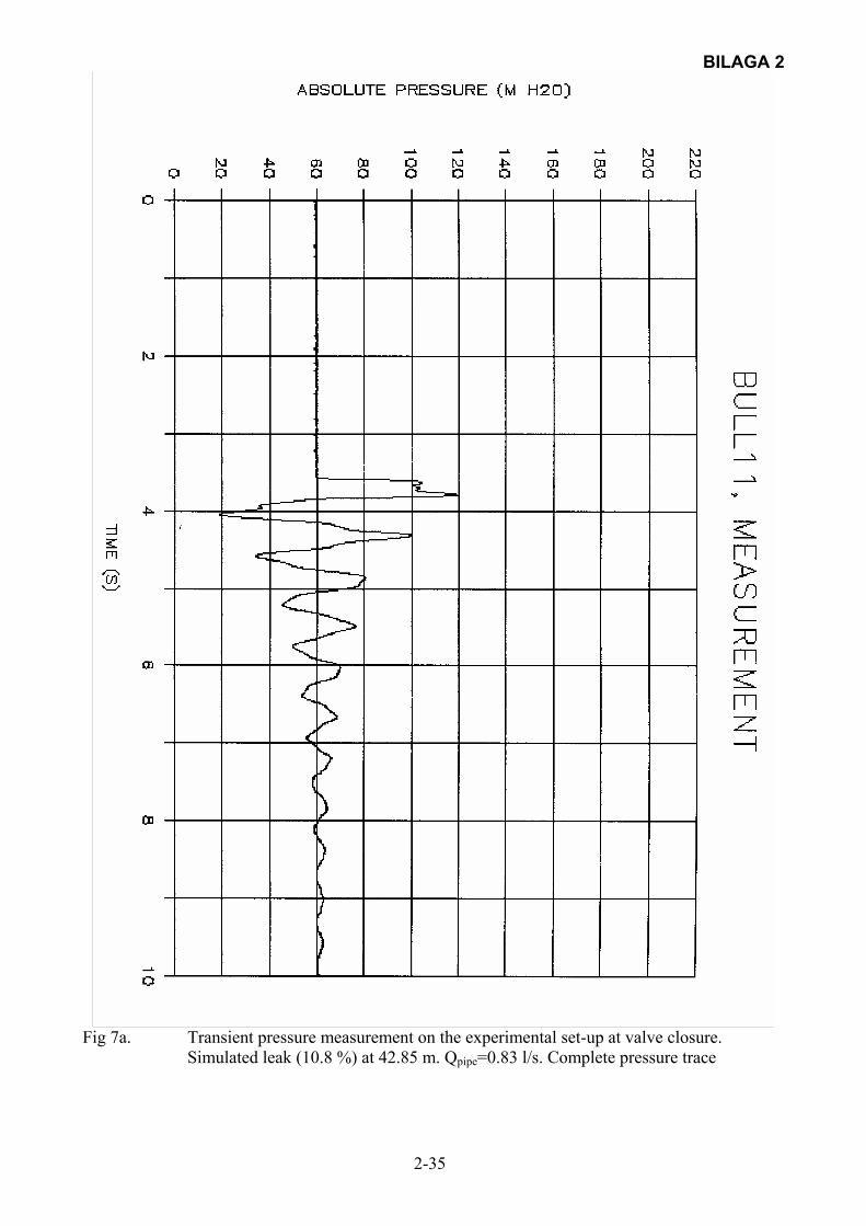
BILAGA 2

2-35

Fig 7a. Transient pressure measurement on the experimental set-up at valve closure.

Simulated leak (10.8 %) at 42.85 m. Qpipe=0.83 l/s. Complete pressure trace

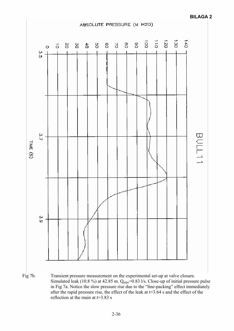
BILAGA 2

2-36

Fig 7b. Transient pressure measurement on the experimental set-up at valve closure.

Simulated leak (10.8 %) at 42.85 m. Qpipe=0.83 l/s. Close-up of initial pressure pulse in Fig 7a. Notice the slow pressure rise due to the “line-packing” effect immediately after the rapid pressure rise, the effect of the leak at t=3.64 s and the effect of the reflection at the main at t=3.83 s

BILAGA 2

2-37

Fig 7c. Computed initial pressure transient for the flow situation shown in Figs 7a,b. Notice

the effect of the leak at t=0.17 s and the reflection from the main at t=0.32 s

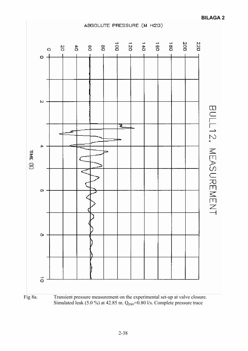
BILAGA 2

2-38

Fig 8a. Transient pressure measurement on the experimental set-up at valve closure.

Simulated leak (5.0 %) at 42.85 m. Qpipe=0.80 l/s. Complete pressure trace

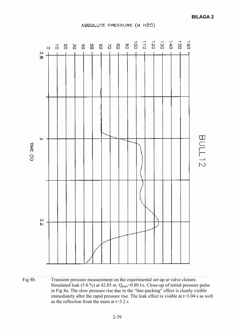
BILAGA 2

2-39

Fig 8b. Transient pressure measurement on the experimental set-up at valve closure.

Simulated leak (5.0 %) at 42.85 m. Qpipe=0.80 l/s. Close-up of initial pressure pulse in Fig 8a. The slow pressure rise due to the “line-packing” effect is clearly visible immediately after the rapid pressure rise. The leak effect is visible at t=3.04 s as well as the reflection from the main at t=3.2 s

BILAGA 2

2-40

Fig 8c. Computed initial pressure transient for the flow situation shown in Figs 8a,b. Notice

the effect of the leak at t=0.16 s and the reflection from the main at t=0.32 s

BILAGA 2

2-41

. Fig 9a Transient pressure measurement on the experimental set-up at valve closure.

Simulated leak (6.8 %) at 42.85 m. Qpipe=0.80 l/s. Complete pressure trace

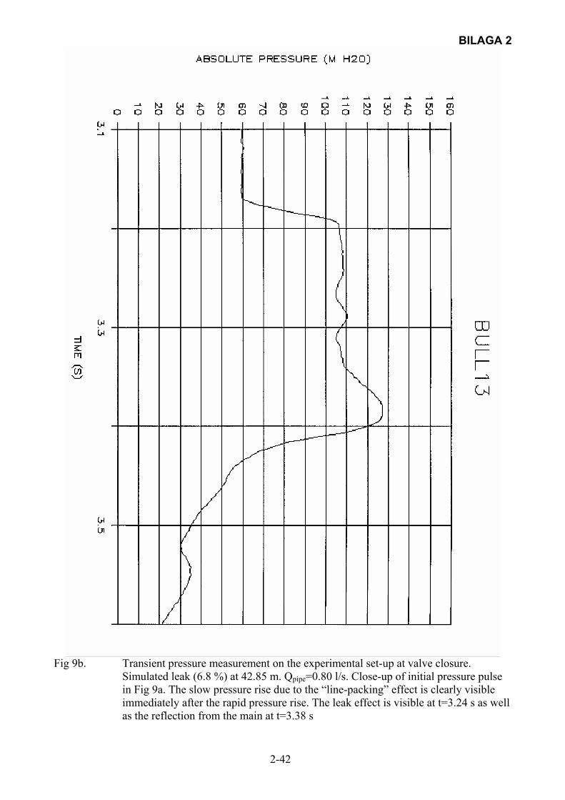
BILAGA 2

2-42

Fig 9b. Transient pressure measurement on the experimental set-up at valve closure.

Simulated leak (6.8 %) at 42.85 m. Qpipe=0.80 l/s. Close-up of initial pressure pulse in Fig 9a. The slow pressure rise due to the “line-packing” effect is clearly visible immediately after the rapid pressure rise. The leak effect is visible at t=3.24 s as well as the reflection from the main at t=3.38 s

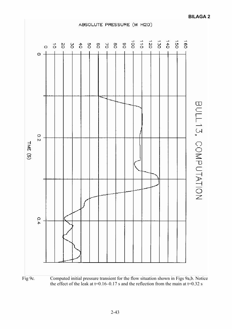
BILAGA 2

2-43

Fig 9c. Computed initial pressure transient for the flow situation shown in Figs 9a,b. Notice

the effect of the leak at t=0.16–0.17 s and the reflection from the main at t=0.32 s

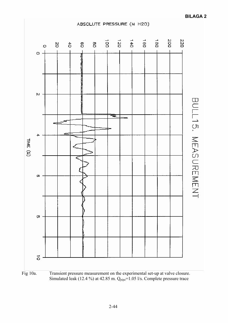
BILAGA 2

2-44

Fig 10a. Transient pressure measurement on the experimental set-up at valve closure.

Simulated leak (12.4 %) at 42.85 m. Qpipe=1.05 l/s. Complete pressure trace

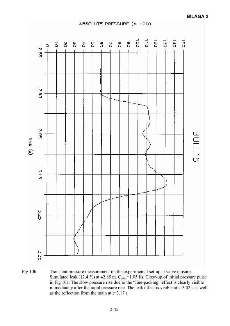
BILAGA 2

2-45

Fig 10b. Transient pressure measurement on the experimental set-up at valve closure.

Simulated leak (12.4 %) at 42.85 m. Qpipe=1.05 l/s. Close-up of initial pressure pulse in Fig 10a. The slow pressure rise due to the “line-packing” effect is clearly visible immediately after the rapid pressure rise. The leak effect is visible at t=3.02 s as well as the reflection from the main at t=3.17 s

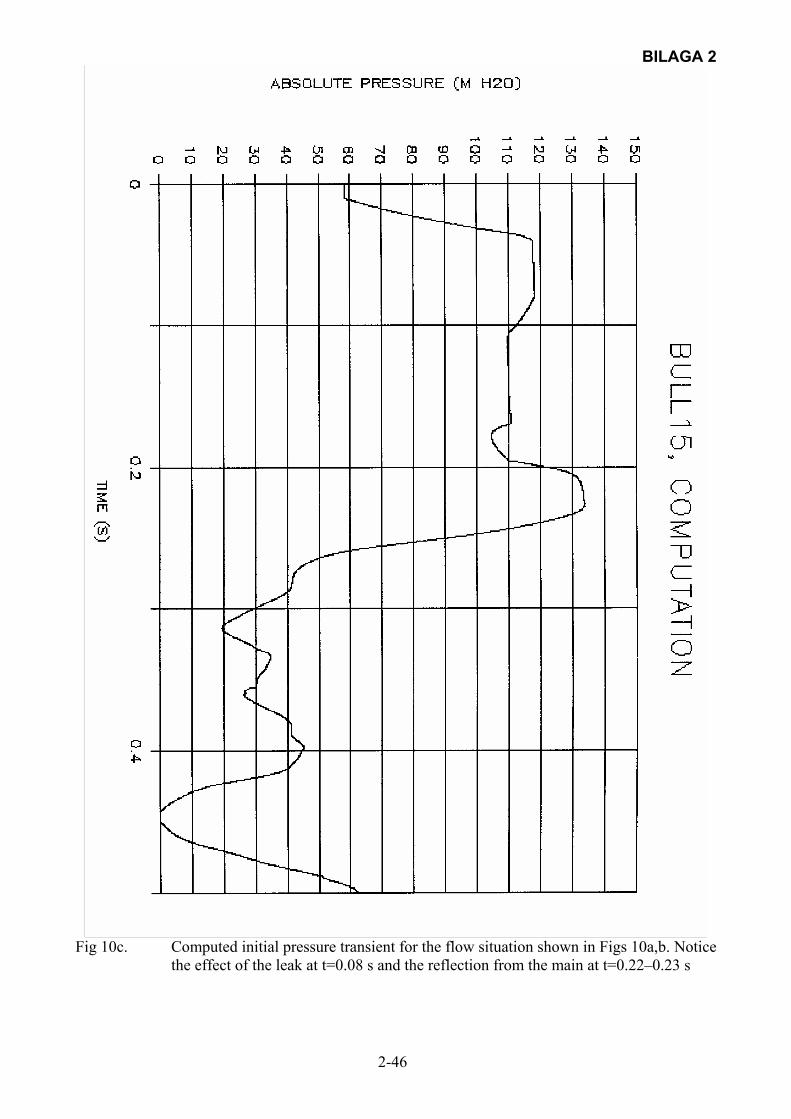
BILAGA 2

2-46

Fig 10c. Computed initial pressure transient for the flow situation shown in Figs 10a,b. Notice

the effect of the leak at t=0.08 s and the reflection from the main at t=0.22–0.23 s

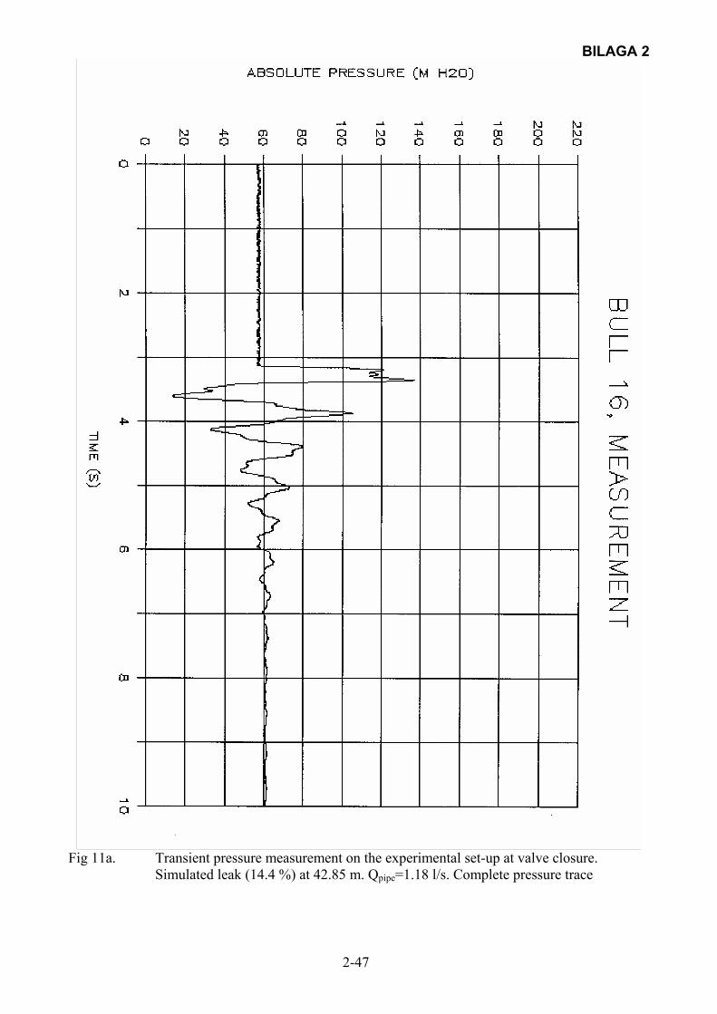
BILAGA 2

2-47

Fig 11a. Transient pressure measurement on the experimental set-up at valve closure.

Simulated leak (14.4 %) at 42.85 m. Qpipe=1.18 l/s. Complete pressure trace

BILAGA 2

2-48

Fig 11b Transient pressure measurement on the experimental set-up at valve closure.

Simulated leak (14.4 %) at 42.85 m. Qpipe=1.18 l/s. Close-up of initial pressure pulse in Fig 11a. The slow pressure rise due to the “line-packing” effect is not very visible immediately after the rapid pressure rise. The leak effect is visible at t=3.20 s as well as the reflection from the main at about t=3.36 s

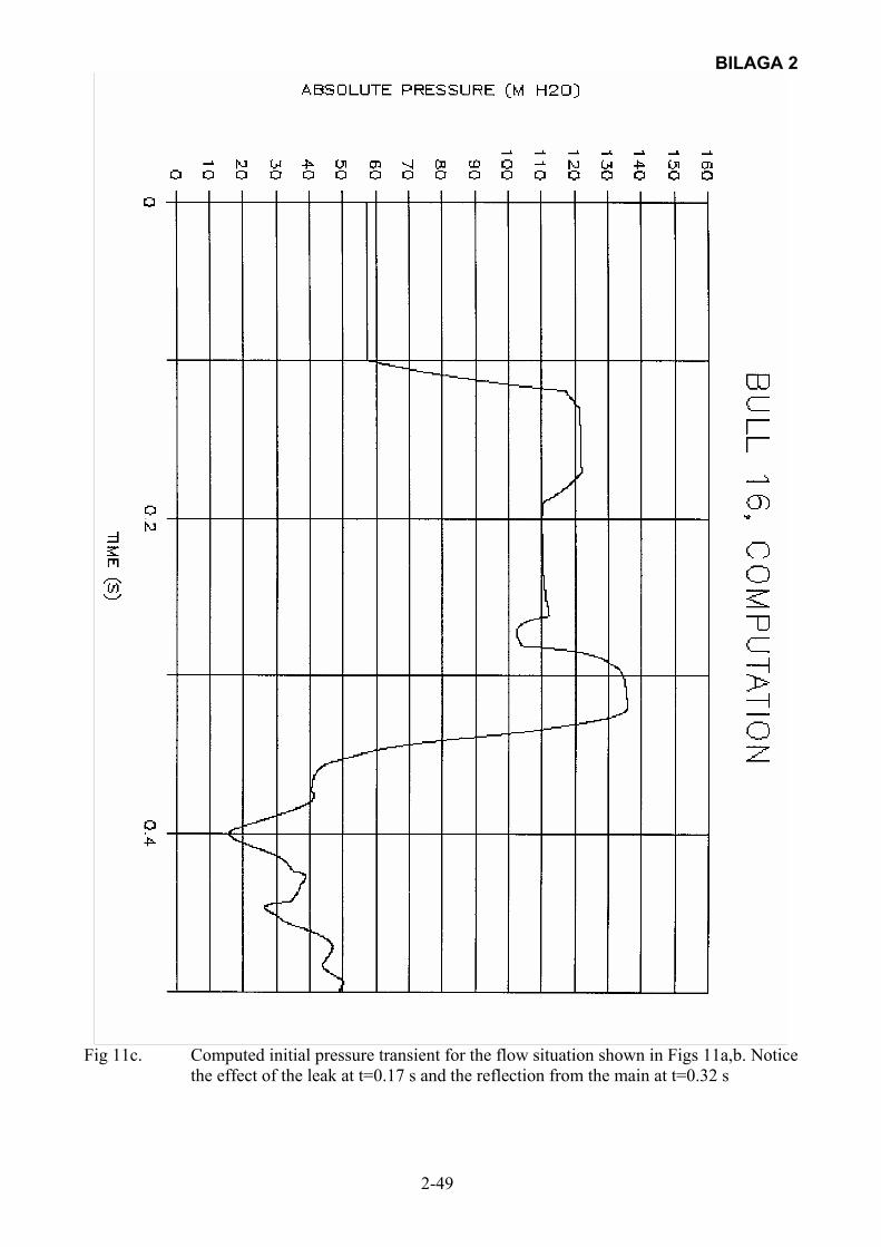
BILAGA 2

2-49

Fig 11c. Computed initial pressure transient for the flow situation shown in Figs 11a,b. Notice

the effect of the leak at t=0.17 s and the reflection from the main at t=0.32 s

BILAGA 2

2-50

Fig 12a. Transient pressure measurement on the experimental set-up at valve closure. No

leak. Complete pressure trace

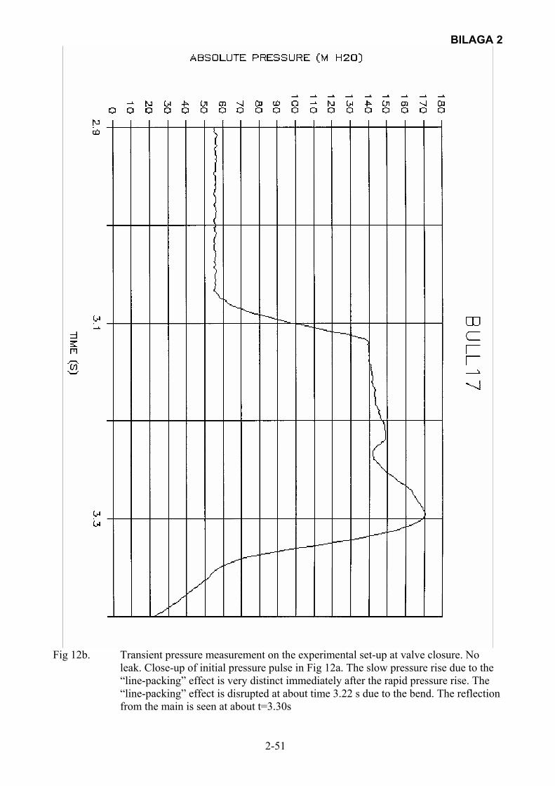
BILAGA 2

2-51

Fig 12b. Transient pressure measurement on the experimental set-up at valve closure. No

leak. Close-up of initial pressure pulse in Fig 12a. The slow pressure rise due to the “line-packing” effect is very distinct immediately after the rapid pressure rise. The “line-packing” effect is disrupted at about time 3.22 s due to the bend. The reflection from the main is seen at about t=3.30s

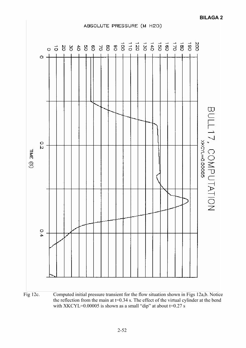
BILAGA 2

2-52

Fig 12c. Computed initial pressure transient for the flow situation shown in Figs 12a,b. Notice

the reflection from the main at t=0.34 s. The effect of the virtual cylinder at the bend with XKCYL=0.00005 is shown as a small “dip” at about t=0.27 s

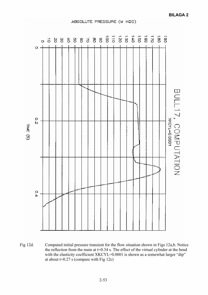
BILAGA 2

2-53

Fig 12d. Computed initial pressure transient for the flow situation shown in Figs 12a,b. Notice

the reflection from the main at t=0.34 s. The effect of the virtual cylinder at the bend with the elasticity coefficient XKCYL=0.0001 is shown as a somewhat larger “dip” at about t=0.27 s (compare with Fig 12c)

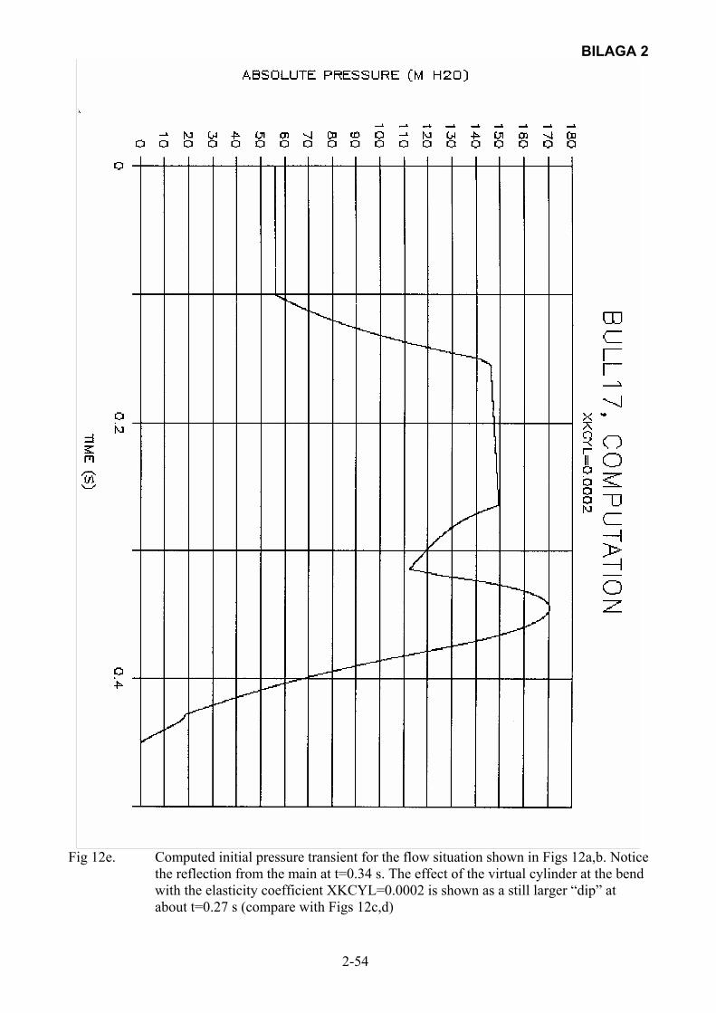
BILAGA 2

2-54

Fig 12e. Computed initial pressure transient for the flow situation shown in Figs 12a,b. Notice

the reflection from the main at t=0.34 s. The effect of the virtual cylinder at the bend with the elasticity coefficient XKCYL=0.0002 is shown as a still larger “dip” at about t=0.27 s (compare with Figs 12c,d)

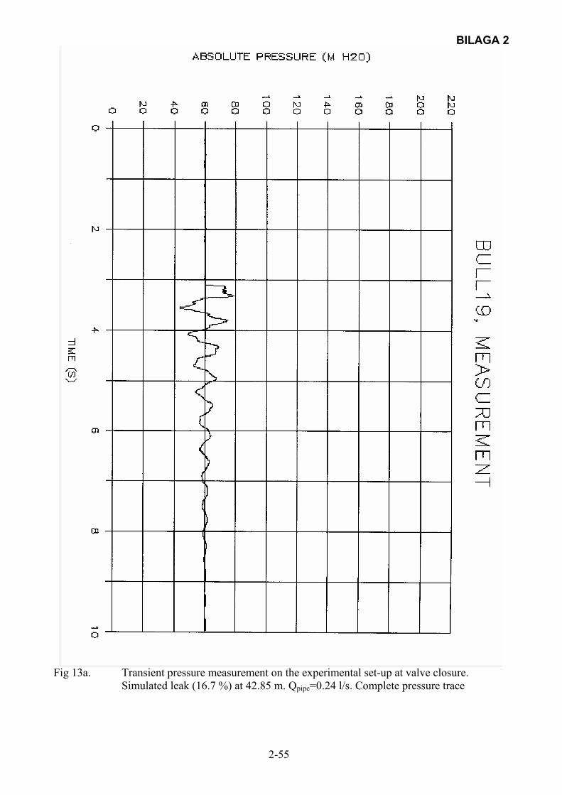
BILAGA 2

2-55

Fig 13a. Transient pressure measurement on the experimental set-up at valve closure.

Simulated leak (16.7 %) at 42.85 m. Qpipe=0.24 l/s. Complete pressure trace

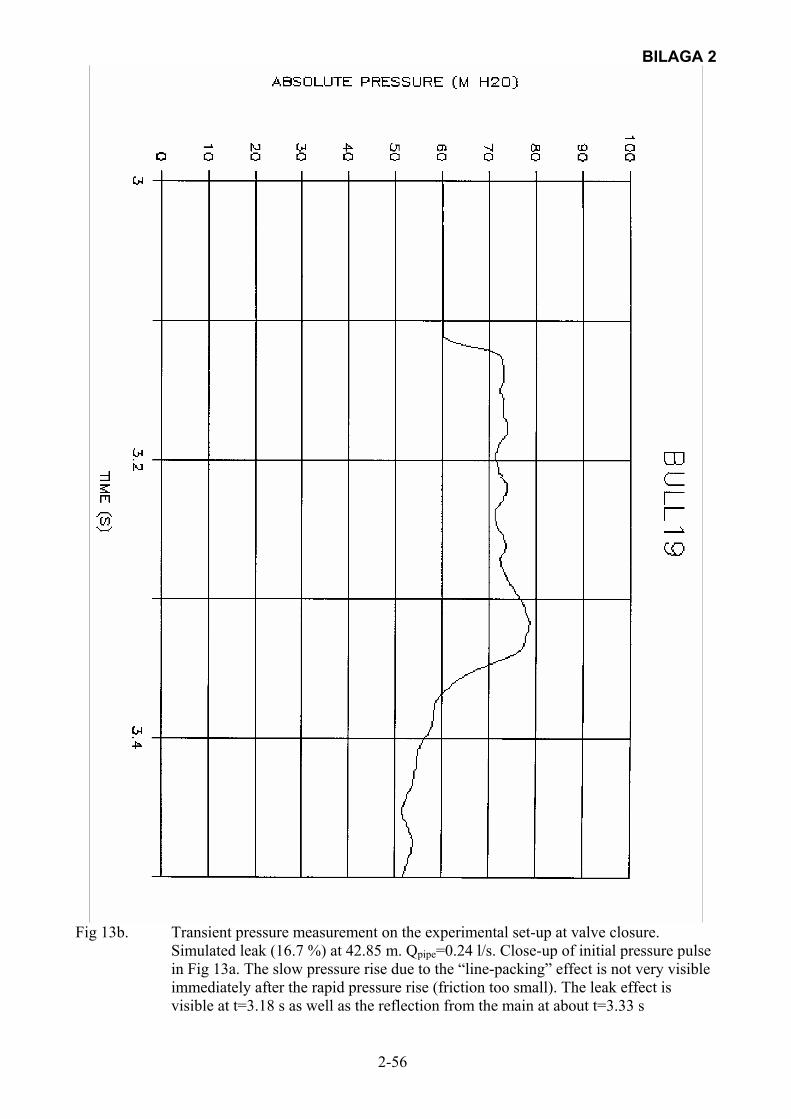
BILAGA 2

2-56

Fig 13b. Transient pressure measurement on the experimental set-up at valve closure.

Simulated leak (16.7 %) at 42.85 m. Qpipe=0.24 l/s. Close-up of initial pressure pulse in Fig 13a. The slow pressure rise due to the “line-packing” effect is not very visible immediately after the rapid pressure rise (friction too small). The leak effect is visible at t=3.18 s as well as the reflection from the main at about t=3.33 s

BILAGA 2

2-57

Fig 13c. Computed initial pressure transient for the flow situation shown in Figs 13a,b. The

effect of the leak at about t=0.17 s is not very visible due to the small pressure pulse. The reflection at the main is distinct at t=0.31 s. The “dip” at t=0.25 s is due to the virtual cylinder (i.e. the bend)

BILAGA 2

2-58

Fig 14a. Transient pressure measurement on the experimental set-up at valve closure.

Simulated leak (4.4 %) at 79.65 m. Qpipe=1.14 l/s. Complete pressure trace

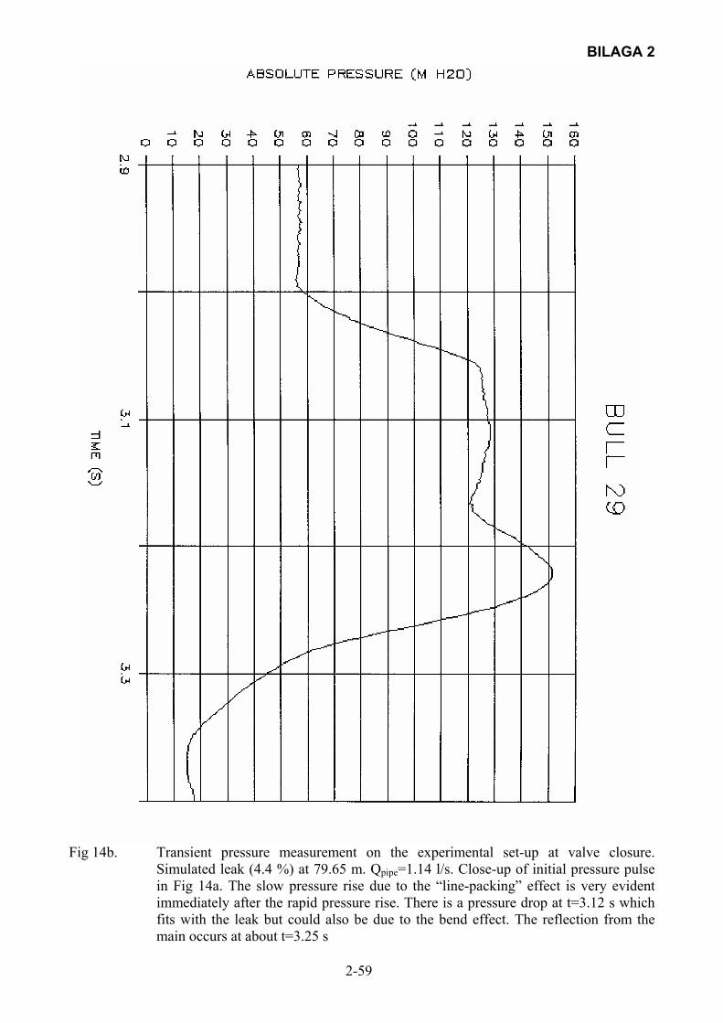
BILAGA 2

2-59

Fig 14b. Transient pressure measurement on the experimental set-up at valve closure.

Simulated leak (4.4 %) at 79.65 m. Qpipe=1.14 l/s. Close-up of initial pressure pulse in Fig 14a. The slow pressure rise due to the “line-packing” effect is very evident immediately after the rapid pressure rise. There is a pressure drop at t=3.12 s which fits with the leak but could also be due to the bend effect. The reflection from the main occurs at about t=3.25 s

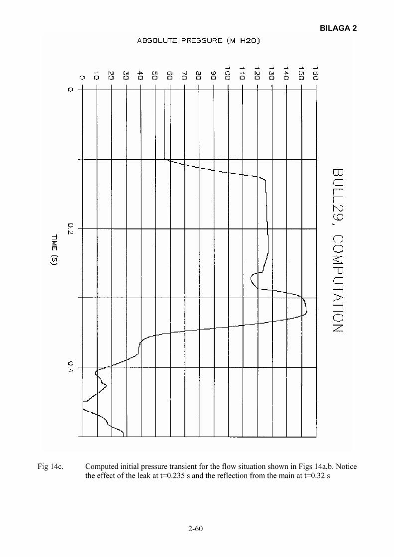
BILAGA 2

2-60

Fig 14c. Computed initial pressure transient for the flow situation shown in Figs 14a,b. Notice

the effect of the leak at t=0.235 s and the reflection from the main at t=0.32 s

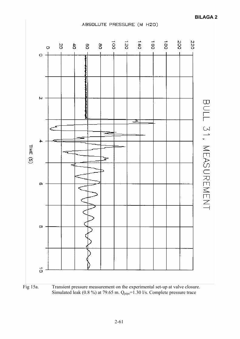
BILAGA 2

2-61

Fig 15a. Transient pressure measurement on the experimental set-up at valve closure.

Simulated leak (0.8 %) at 79.65 m. Qpipe=1.30 l/s. Complete pressure trace

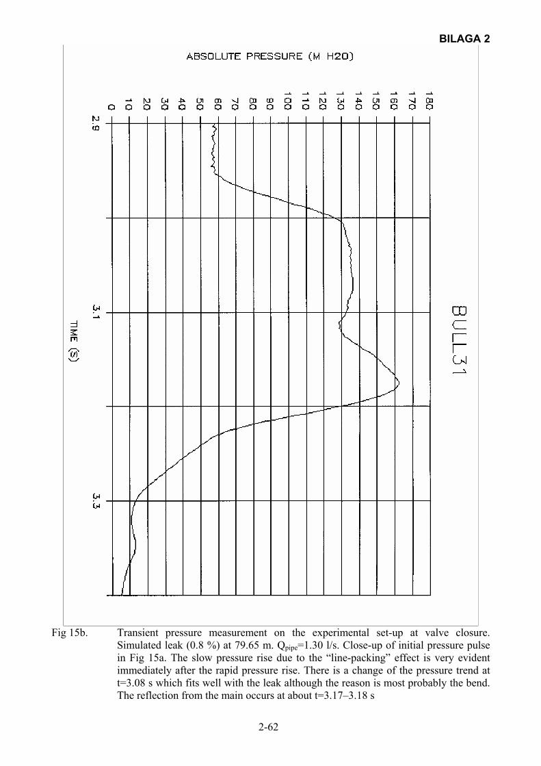
BILAGA 2

2-62

Fig 15b. Transient pressure measurement on the experimental set-up at valve closure.

Simulated leak (0.8 %) at 79.65 m. Qpipe=1.30 l/s. Close-up of initial pressure pulse in Fig 15a. The slow pressure rise due to the “line-packing” effect is very evident immediately after the rapid pressure rise. There is a change of the pressure trend at t=3.08 s which fits well with the leak although the reason is most probably the bend. The reflection from the main occurs at about t=3.17–3.18 s

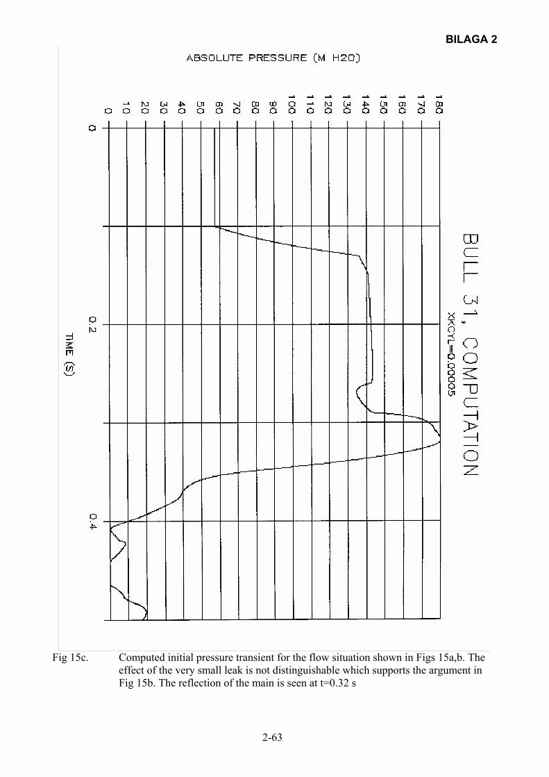
BILAGA 2

2-63

Fig 15c. Computed initial pressure transient for the flow situation shown in Figs 15a,b. The

effect of the very small leak is not distinguishable which supports the argument in Fig 15b. The reflection of the main is seen at t=0.32 s

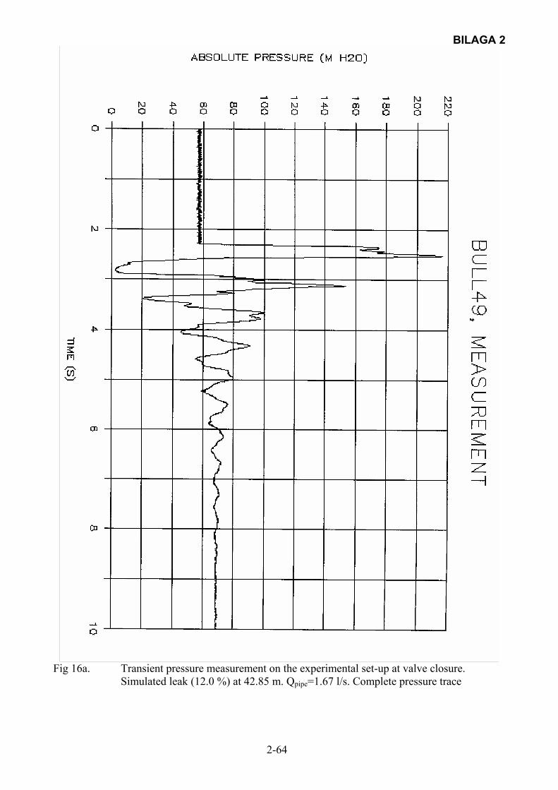
BILAGA 2

2-64

Fig 16a. Transient pressure measurement on the experimental set-up at valve closure.

Simulated leak (12.0 %) at 42.85 m. Qpipe=1.67 l/s. Complete pressure trace

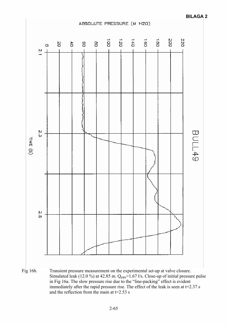
BILAGA 2

2-65

Fig 16b. Transient pressure measurement on the experimental set-up at valve closure.

Simulated leak (12.0 %) at 42.85 m. Qpipe=1.67 l/s. Close-up of initial pressure pulse in Fig 16a. The slow pressure rise due to the “line-packing” effect is evident immediately after the rapid pressure rise. The effect of the leak is seen at t=2.37 s and the reflection from the main at t=2.53 s

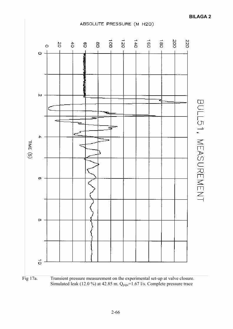
BILAGA 2

2-66

Fig 17a. Transient pressure measurement on the experimental set-up at valve closure.

Simulated leak (12.0 %) at 42.85 m. Qpipe=1.67 l/s. Complete pressure trace

BILAGA 2

2-67

Fig 17b. Transient pressure measurement on the experimental set-up at a relatively slow valve

closure. Simulated leak (12.0 %) at 42.85 m. Qpipe=1.67 l/s. Close-up of initial pressure pulse in Fig 17a. No “line-packing” effect. The slow valve closure makes it difficult to distinguish the leak. There is, however, a small pressure change at t=2.181 s which is attributed to the leak. The reflection from the main is seen at about t=2.34 s

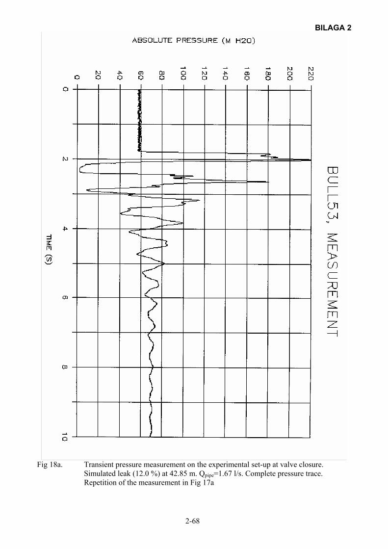
BILAGA 2

2-68

Fig 18a. Transient pressure measurement on the experimental set-up at valve closure.

Simulated leak (12.0 %) at 42.85 m. Qpipe=1.67 l/s. Complete pressure trace. Repetition of the measurement in Fig 17a

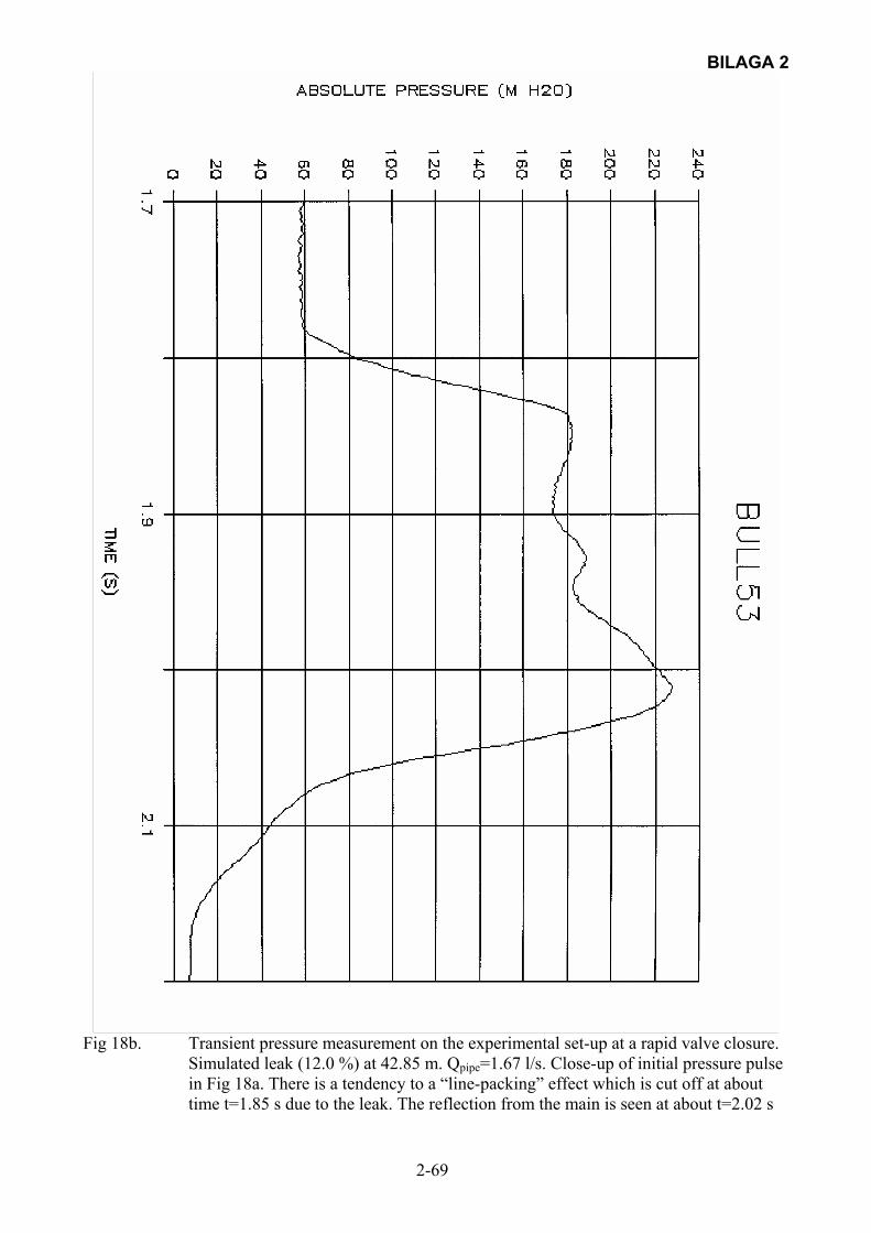
BILAGA 2

2-69

Fig 18b. Transient pressure measurement on the experimental set-up at a rapid valve closure.

Simulated leak (12.0 %) at 42.85 m. Qpipe=1.67 l/s. Close-up of initial pressure pulse in Fig 18a. There is a tendency to a “line-packing” effect which is cut off at about time t=1.85 s due to the leak. The reflection from the main is seen at about t=2.02 s

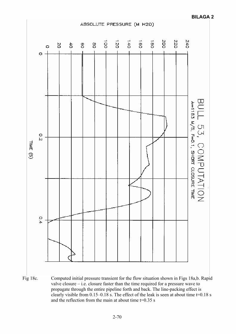
BILAGA 2

2-70

Fig 18c. Computed initial pressure transient for the flow situation shown in Figs 18a,b. Rapid

valve closure – i.e. closure faster than the time required for a pressure wave to propagate through the entire pipeline forth and back. The line-packing effect is clearly visible from 0.15–0.18 s. The effect of the leak is seen at about time t=0.18 s and the reflection from the main at about time t=0.35 s

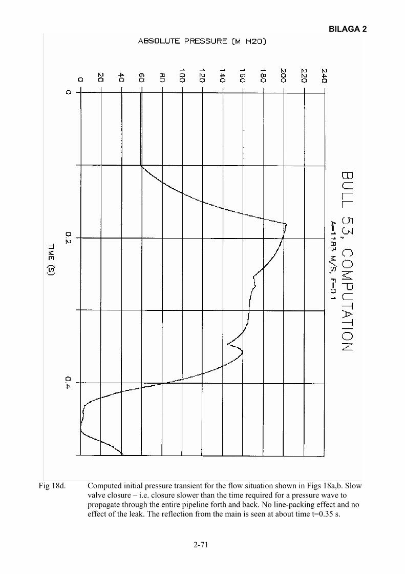
BILAGA 2

2-71

Fig 18d. Computed initial pressure transient for the flow situation shown in Figs 18a,b. Slow

valve closure – i.e. closure slower than the time required for a pressure wave to propagate through the entire pipeline forth and back. No line-packing effect and no effect of the leak. The reflection from the main is seen at about time t=0.35 s.

BILAGA 2

2-72

Fig 19a. Transient pressure measurement on the experimental set-up at valve closure.

Simulated leak (4.8 %) at 42.85 m. Qpipe=1.67 l/s. Complete pressure trace.

BILAGA 2

2-73

Fig 19b. Transient pressure measurement on the experimental set-up at a rapid valve closure.

Simulated leak (4.8 %) at 42.85 m. Qpipe=1.67 l/s. Close-up of initial pressure pulse in Fig 19a. The relatively noisy signal and the small leak makes it impossible to detect the effect of the leak. Reflection from the main at about time t=2.48 s

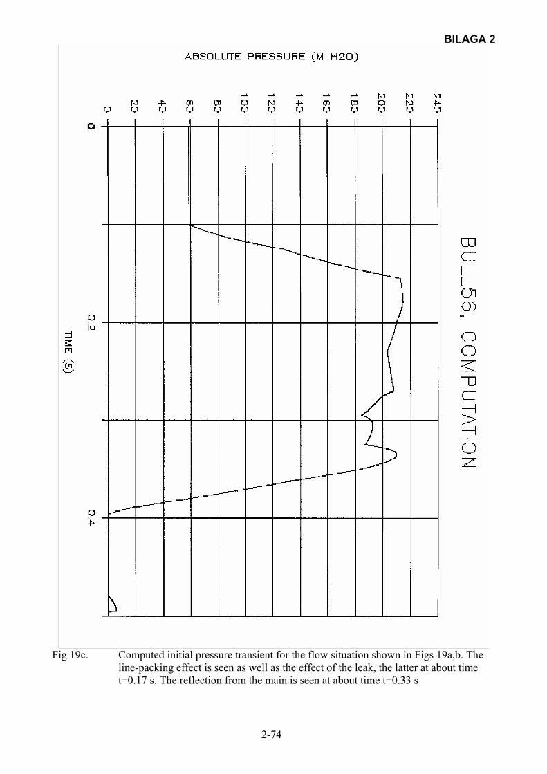
BILAGA 2

2-74

Fig 19c. Computed initial pressure transient for the flow situation shown in Figs 19a,b. The

line-packing effect is seen as well as the effect of the leak, the latter at about time t=0.17 s. The reflection from the main is seen at about time t=0.33 s

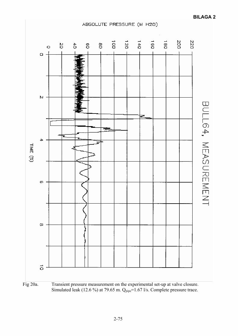
BILAGA 2

2-75

Fig 20a. Transient pressure measurement on the experimental set-up at valve closure.

Simulated leak (12.6 %) at 79.65 m. Qpipe=1.67 l/s. Complete pressure trace.

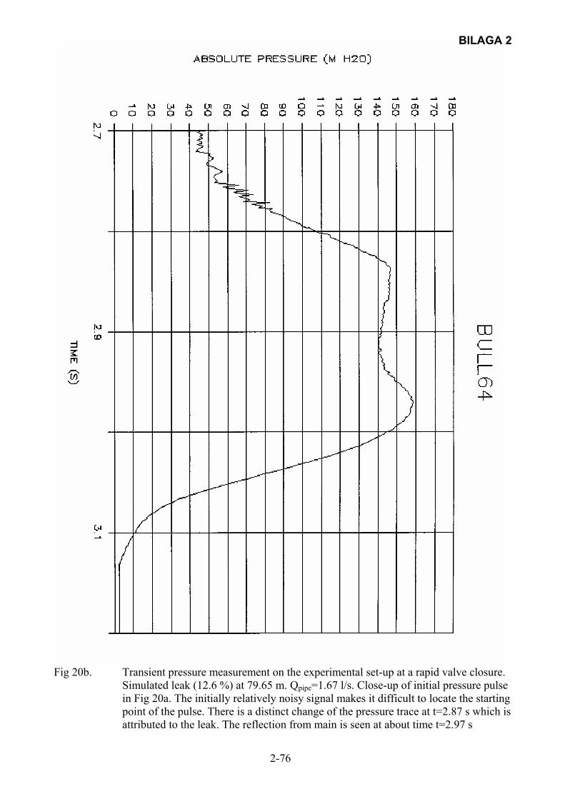
BILAGA 2

2-76

Fig 20b. Transient pressure measurement on the experimental set-up at a rapid valve closure.

Simulated leak (12.6 %) at 79.65 m. Qpipe=1.67 l/s. Close-up of initial pressure pulse in Fig 20a. The initially relatively noisy signal makes it difficult to locate the starting point of the pulse. There is a distinct change of the pressure trace at t=2.87 s which is attributed to the leak. The reflection from main is seen at about time t=2.97 s

BILAGA 2

2-77

Fig 20c. Computed initial pressure transient for the flow situation shown in Figs 20a,b. The

effect of the large leak is seen very clearly at time t=0.245 s. The reflection from the main is barely visible at time t=0.33 s

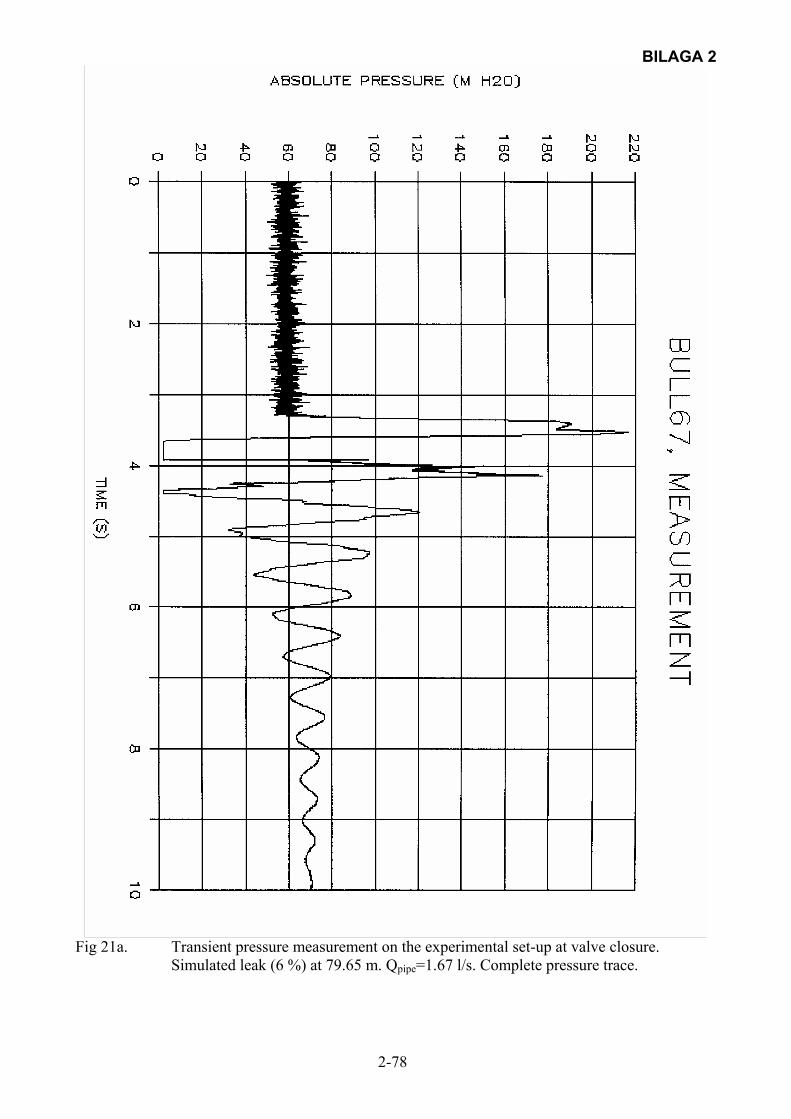
BILAGA 2

2-78

Fig 21a. Transient pressure measurement on the experimental set-up at valve closure.

Simulated leak (6 %) at 79.65 m. Qpipe=1.67 l/s. Complete pressure trace.

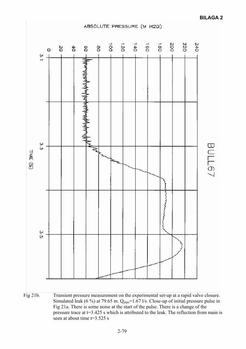
BILAGA 2

2-79

Fig 21b. Transient pressure measurement on the experimental set-up at a rapid valve closure.

Simulated leak (6 %) at 79.65 m. Qpipe=1.67 l/s. Close-up of initial pressure pulse in Fig 21a. There is some noise at the start of the pulse. There is a change of the pressure trace at t=3.425 s which is attributed to the leak. The reflection from main is seen at about time t=3.525 s

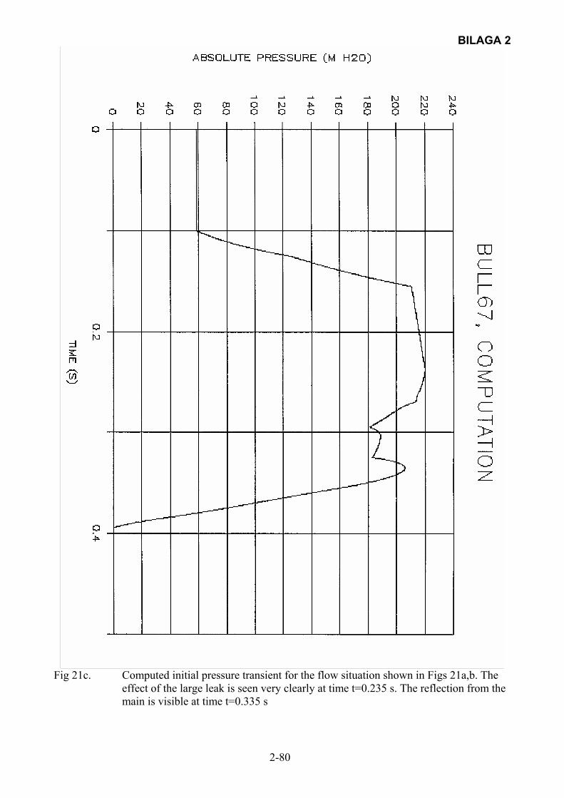
BILAGA 2

2-80

Fig 21c. Computed initial pressure transient for the flow situation shown in Figs 21a,b. The

effect of the large leak is seen very clearly at time t=0.235 s. The reflection from the main is visible at time t=0.335 s

BILAGA 2

2-81

Fig 22. Pipeline used for theoretical calculations of the effect of a leak on transients in

conjunction with spectral analysis of the transient pressure. The upstream end is equipped with a pump and a shut-off valve. Transients are generated through pump stop and valve closure. The leak is located at the distance L1

Fig 23. Calculation of the pressure transient at pump stop and valve closure. No leak

BILAGA 2

2-82

Fig 24 Frequency spectra for the transient shown in Fig 23 – no leak Top: Spectrum calculated from data points 1,100–3,148 Bottom: Spectrum calculated from data points 1,400–3,448

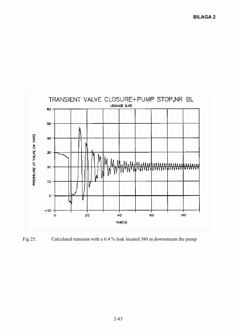
BILAGA 2

2-83

Fig 25. Calculated transient with a 6.4 % leak located 380 m downstream the pump

BILAGA 2

2-84

Fig 26. Frequency spectra for the transient shown in Fig 25 – with a 6.4 % leak Top: Spectrum calculated from data points 1,000–3,048 Bottom: Spectrum calculated from data points 2,400–4,448

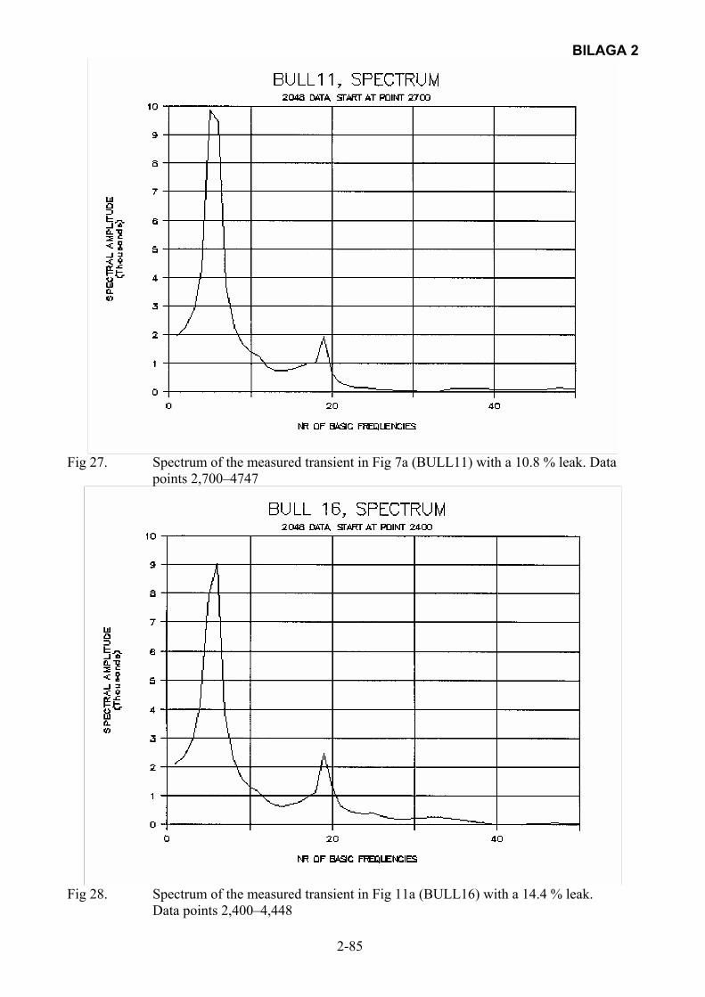
BILAGA 2

2-85

Fig 27. Spectrum of the measured transient in Fig 7a (BULL11) with a 10.8 % leak. Data

points 2,700–4747

Fig 28. Spectrum of the measured transient in Fig 11a (BULL16) with a 14.4 % leak. Data points 2,400–4,448

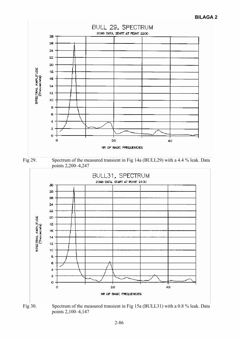
BILAGA 2

2-86

Fig 29. Spectrum of the measured transient in Fig 14a (BULL29) with a 4.4 % leak. Data

points 2,200–4,247

Fig 30. Spectrum of the measured transient in Fig 15a (BULL31) with a 0.8 % leak. Data

points 2,100–4,147

BILAGA 2

2-87

APPENDIX 1 Computer program TRBULL.FOR for transient calculations in a pipeline with a leak C THIS PROGRAM CALCULATES THE PRESSURE TRANSIENT IN THE EXPERI- C MENTAL SET-UP AT BULLTOFTA WITH SIMULATED LEAKS AND RAPID C BALL VALVE CLOSURE - SEE REPORT VA-FORSK CONCERNING THE SET-UP C DIMENSION H(1:5000),H1(1:5000),Q(1:5000),Q1(1:5000),HCP(1:5000), &HCM(1:5000) COMMON/VENTST/DIA2,AREA2,XKONST0,T0,T1,T2,XVENT1,XKVV0,XLAGE1, &XLAGE0 OPEN(UNIT=7,FILE='TRBULLIN.DAT',STATUS='OLD') OPEN(UNIT=8,FILE='TRBULLUT.DAT',STATUS='OLD') READ(7,*)XL1,XL2,DIA1,DIA2,FRIK,VAGH READ(7,*)QPIPE,QLAECK,H0VALVE,ACYL,XKCYL READ(7,*)T0,T1,T2,TIDSLUT,XKONST0,XVENT1 READ(7,*)N,XLAECK C C CALCULATION OF CONSTANTS C XKVV0=H0VALVE/(QPIPE-QLAECK)**2 WRITE(*,*)'XKVV0=',XKVV0 AREA1=3.14/4*DIA1**2 AREA2=3.14/4*DIA2**2 VEL1=QPIPE/AREA1 VEL2A=QPIPE/AREA2 VEL2B=(QPIPE-QLAECK)/AREA2 B1=VAGH/9.81/AREA1 B2=VAGH/9.81/AREA2 DELTX=(XL1+XL2)/(N-1) DELTT=DELTX/VAGH R1=FRIK*DELTX/19.62/DIA1/AREA1**2 R2=FRIK*DELTX/19.62/DIA2/AREA2**2 M=XL1/DELTX+1 XL1NY=DELTX*(M-1) XL2NY=DELTX*(N-M) LL=XLAECK/DELTX LX=N-LL XLAECKNY=LL*DELTX XXD1=SQRT(XKVV0/XKONST0) XLAGE0=DIA2-DIA2/(1+XXD1) WRITE(*,*)'XLAGE0=',XLAGE0 TID=0 WRITE(8,*)' TID H1(N) Q1L' C C STEADY STATE C HF1=FRIK*XL1NY/DIA1*VEL1**2/19.62 HF2=FRIK*(XL2NY-XLAECKNY)/DIA2*VEL2A**2/19.62 HF3=FRIK*XLAECKNY/DIA2*VEL2B**2/19.62 HMAIN=H0VALVE+HF1+HF2+HF3 WRITE(*,*)'HMAIN=',HMAIN WRITE(*,*)'HF1,HF2,HF3,XL1NY,XL2NY,XLAECKNY',HF1,HF2,HF3, &XL1NY,XL2NY,XLAECKNY DO 100 I=1,M H(I)=HMAIN-(I-1)*HF1/(M-1) Q(I)=QPIPE 100 CONTINUE HM1=H(M) HM2=HM1 QM1=QPIPE

BILAGA 2

2-88

QM2=QPIPE DO 110 I=M,LX-1 H(I)=HM2-(I-M)*HF2/(LX-M) Q(I)=QPIPE 110 CONTINUE HLX1=HM2-HF2 HLX2=HLX1 HLX10=HLX1 QLX1=QPIPE QLX2=QPIPE-QLAECK DO 120 I=LX+1,N H(I)=HLX2-(I-LX)*HF3/(N-LX) Q(I)=QPIPE-QLAECK 120 CONTINUE WRITE(*,*)'H(N)=',H(N) XKLX0=HLX1/QLAECK**2 WRITE(*,*)'XKLX=',XKLX WRITE(*,*)'LX=',LX C C TRANSIENT PHASE, INNER POINTS AND BOUNDARY POINTS, OLD C TIME STEP C 720 DO 200 I=1,M HCP(I)=H(I)+B1*Q(I)-R1*Q(I)*ABS(Q(I)) HCM(I)=H(I)-B1*Q(I)+R1*Q(I)*ABS(Q(I)) 200 CONTINUE HCMM1=HM1-B1*QM1+R1*QM1*ABS(QM1) DO 210 I=M,LX HCP(I)=H(I)+B2*Q(I)-R2*Q(I)*ABS(Q(I)) HCM(I)=H(I)-B2*Q(I)+R2*Q(I)*ABS(Q(I)) 210 CONTINUE HCPM2=HM2+B2*QM2-R2*QM2*ABS(QM2) HCMLX1=HLX1-B2*QLX1+R2*QLX1*ABS(QLX1) DO 220 I=M,N HCP(I)=H(I)+B2*Q(I)-R2*Q(I)*ABS(Q(I)) HCM(I)=H(I)-B2*Q(I)+R2*Q(I)*ABS(Q(I)) 220 CONTINUE HCPLX2=HLX2+B2*QLX2-R2*QLX2*ABS(QLX2) C C TRANSIENT PHASE, INNER POINTS, NEW TIME STEP C DO 300 I=2,M-2 H1(I)=(HCP(I-1)+HCM(I+1))/2 Q1(I)=(H1(I)-HCM(I+1))/B1 300 CONTINUE H1(M-1)=(HCP(M-2)+HCMM1)/2 Q1(M-1)=(H1(M-1)-HCMM1)/B1 DO 310 I=M+2,LX-2 H1(I)=(HCP(I-1)+HCM(I+1))/2 Q1(I)=(H1(I)-HCM(I+1))/B2 310 CONTINUE H1(M+1)=(HCPM2+HCM(M+2))/2 Q1(M+1)=(H1(M+1)-HCM(M+2))/B2 H1(LX-1)=(HCP(LX-2)+HCMLX1)/2 Q1(LX-1)=(H1(LX-1)-HCMLX1)/B2 DO 320 I=LX+2,N-1 H1(I)=(HCP(I-1)+HCM(I+1))/2 Q1(I)=(H1(I)-HCM(I+1))/B2 320 CONTINUE H1(LX+1)=(HCPLX2+HCM(LX+2))/2 Q1(LX+1)=(H1(LX+1)-HCM(LX+2))/B2 C C TRANSIENT PHASE, BOUNDARIES C

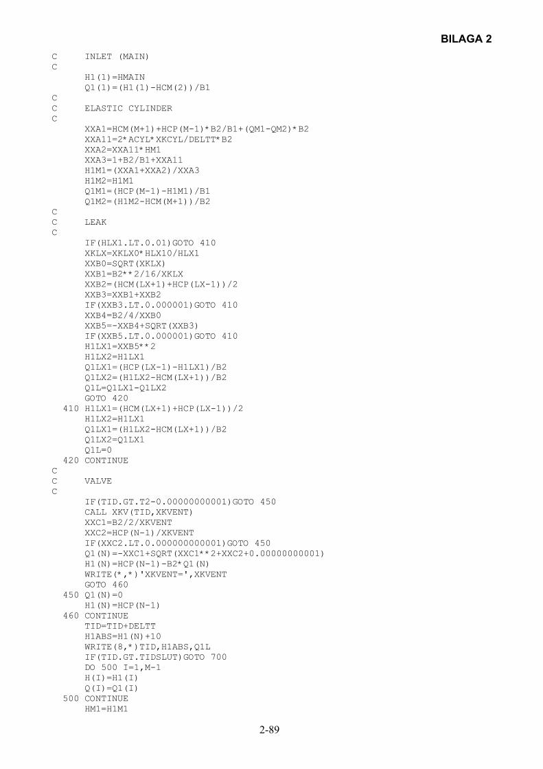
BILAGA 2

2-89

C INLET (MAIN) C H1(1)=HMAIN Q1(1)=(H1(1)-HCM(2))/B1 C C ELASTIC CYLINDER C XXA1=HCM(M+1)+HCP(M-1)*B2/B1+(QM1-QM2)*B2 XXA11=2*ACYL*XKCYL/DELTT*B2 XXA2=XXA11*HM1 XXA3=1+B2/B1+XXA11 H1M1=(XXA1+XXA2)/XXA3 H1M2=H1M1 Q1M1=(HCP(M-1)-H1M1)/B1 Q1M2=(H1M2-HCM(M+1))/B2 C C LEAK C IF(HLX1.LT.0.01)GOTO 410 XKLX=XKLX0*HLX10/HLX1 XXB0=SQRT(XKLX) XXB1=B2**2/16/XKLX XXB2=(HCM(LX+1)+HCP(LX-1))/2 XXB3=XXB1+XXB2 IF(XXB3.LT.0.000001)GOTO 410 XXB4=B2/4/XXB0 XXB5=-XXB4+SQRT(XXB3) IF(XXB5.LT.0.000001)GOTO 410 H1LX1=XXB5**2 H1LX2=H1LX1 Q1LX1=(HCP(LX-1)-H1LX1)/B2 Q1LX2=(H1LX2-HCM(LX+1))/B2 Q1L=Q1LX1-Q1LX2 GOTO 420 410 H1LX1=(HCM(LX+1)+HCP(LX-1))/2 H1LX2=H1LX1 Q1LX1=(H1LX2-HCM(LX+1))/B2 Q1LX2=Q1LX1 Q1L=0 420 CONTINUE C C VALVE C IF(TID.GT.T2-0.00000000001)GOTO 450 CALL XKV(TID,XKVENT) XXC1=B2/2/XKVENT XXC2=HCP(N-1)/XKVENT IF(XXC2.LT.0.000000000001)GOTO 450 Q1(N)=-XXC1+SQRT(XXC1**2+XXC2+0.00000000001) H1(N)=HCP(N-1)-B2*Q1(N) WRITE(*,*)'XKVENT=',XKVENT GOTO 460 450 Q1(N)=0 H1(N)=HCP(N-1) 460 CONTINUE TID=TID+DELTT H1ABS=H1(N)+10 WRITE(8,*)TID,H1ABS,Q1L IF(TID.GT.TIDSLUT)GOTO 700 DO 500 I=1,M-1 H(I)=H1(I) Q(I)=Q1(I) 500 CONTINUE HM1=H1M1

BILAGA 2

2-90

HM2=H1M2 QM1=Q1M1 QM2=Q1M2 DO 510 I=M+1,LX-1 H(I)=H1(I) Q(I)=Q1(I) 510 CONTINUE HLX1=H1LX1 HLX2=H1LX2 QLX1=Q1LX1 QLX2=Q1LX2 DO 520 I=LX+1,N H(I)=H1(I) Q(I)=Q1(I) 520 CONTINUE GOTO 720 700 CONTINUE END C C SUBROUTINE XKV C SUBROUTINE XKV(TIME,XKVV) COMMON/VENTST/DIA2,AREA2,XKONST0,T0,T1,T2,XVENT1,XKVV0,XLAGE1, &XLAGE0 IF(TIME.GT.T0)GOTO 600 XKVV=XKVV0 GOTO 620 600 CONTINUE IF(TIME.GT.T1)GOTO 610 XLAGE=XLAGE0+(XVENT1-XLAGE0)*(TIME-T0)/(T1-T0) AOPP=(DIA2-XLAGE)/DIA2*AREA2 XKVV=(AREA2/AOPP-1)**2*XKONST0 GOTO 620 610 CONTINUE XLAGE=XVENT1+(DIA2-XVENT1)*(TIME-T1)/(T2-T1) AOPP=(DIA2-XLAGE)/DIA2*AREA2 XKVV=(AREA2/AOPP-1)**2*XKONST0 620 CONTINUE RETURN END

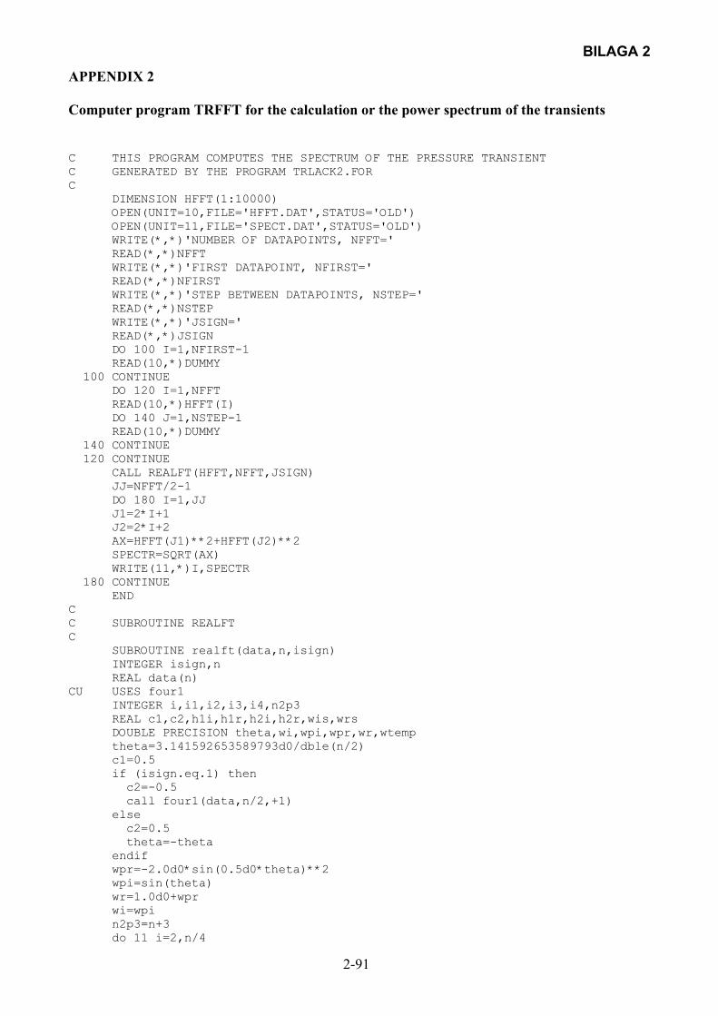
BILAGA 2

2-91

APPENDIX 2 Computer program TRFFT for the calculation or the power spectrum of the transients C THIS PROGRAM COMPUTES THE SPECTRUM OF THE PRESSURE TRANSIENT C GENERATED BY THE PROGRAM TRLACK2.FOR C DIMENSION HFFT(1:10000) OPEN(UNIT=10,FILE='HFFT.DAT',STATUS='OLD') OPEN(UNIT=11,FILE='SPECT.DAT',STATUS='OLD') WRITE(*,*)'NUMBER OF DATAPOINTS, NFFT=' READ(*,*)NFFT WRITE(*,*)'FIRST DATAPOINT, NFIRST=' READ(*,*)NFIRST WRITE(*,*)'STEP BETWEEN DATAPOINTS, NSTEP=' READ(*,*)NSTEP WRITE(*,*)'JSIGN=' READ(*,*)JSIGN DO 100 I=1,NFIRST-1 READ(10,*)DUMMY 100 CONTINUE DO 120 I=1,NFFT READ(10,*)HFFT(I) DO 140 J=1,NSTEP-1 READ(10,*)DUMMY 140 CONTINUE 120 CONTINUE CALL REALFT(HFFT,NFFT,JSIGN) JJ=NFFT/2-1 DO 180 I=1,JJ J1=2*I+1 J2=2*I+2 AX=HFFT(J1)**2+HFFT(J2)**2 SPECTR=SQRT(AX) WRITE(11,*)I,SPECTR 180 CONTINUE END C C SUBROUTINE REALFT C SUBROUTINE realft(data,n,isign) INTEGER isign,n REAL data(n) CU USES four1 INTEGER i,i1,i2,i3,i4,n2p3 REAL c1,c2,h1i,h1r,h2i,h2r,wis,wrs DOUBLE PRECISION theta,wi,wpi,wpr,wr,wtemp theta=3.141592653589793d0/dble(n/2) c1=0.5 if (isign.eq.1) then c2=-0.5 call four1(data,n/2,+1) else c2=0.5 theta=-theta endif wpr=-2.0d0*sin(0.5d0*theta)**2 wpi=sin(theta) wr=1.0d0+wpr wi=wpi n2p3=n+3 do 11 i=2,n/4

BILAGA 2

2-92

i1=2*i-1 i2=i1+1 i3=n2p3-i2 i4=i3+1 wrs=sngl(wr) wis=sngl(wi) h1r=c1*(data(i1)+data(i3)) h1i=c1*(data(i2)-data(i4)) h2r=-c2*(data(i2)+data(i4)) h2i=c2*(data(i1)-data(i3)) data(i1)=h1r+wrs*h2r-wis*h2i data(i2)=h1i+wrs*h2i+wis*h2r data(i3)=h1r-wrs*h2r+wis*h2i data(i4)=-h1i+wrs*h2i+wis*h2r wtemp=wr wr=wr*wpr-wi*wpi+wr wi=wi*wpr+wtemp*wpi+wi 11 continue if (isign.eq.1) then h1r=data(1) data(1)=h1r+data(2) data(2)=h1r-data(2) else h1r=data(1) data(1)=c1*(h1r+data(2)) data(2)=c1*(h1r-data(2)) call four1(data,n/2,-1) endif return END C C SUBROUTINE FOUR1 C C (C) Copr. 1986-92 Numerical Recipes Software ]'.53Y231.. SUBROUTINE four1(data,nn,isign) INTEGER isign,nn REAL data(2*nn) INTEGER i,istep,j,m,mmax,n REAL tempi,tempr DOUBLE PRECISION theta,wi,wpi,wpr,wr,wtemp n=2*nn j=1 do 11 i=1,n,2 if(j.gt.i)then tempr=data(j) tempi=data(j+1) data(j)=data(i) data(j+1)=data(i+1) data(i)=tempr data(i+1)=tempi endif m=n/2 1 if ((m.ge.2).and.(j.gt.m)) then j=j-m m=m/2 goto 1 endif j=j+m 11 continue mmax=2

BILAGA 2

2-93

2 if (n.gt.mmax) then istep=2*mmax theta=6.28318530717959d0/(isign*mmax) wpr=-2.d0*sin(0.5d0*theta)**2 wpi=sin(theta) wr=1.d0 wi=0.d0 do 13 m=1,mmax,2 do 12 i=m,n,istep j=i+mmax tempr=sngl(wr)*data(j)-sngl(wi)*data(j+1) tempi=sngl(wr)*data(j+1)+sngl(wi)*data(j) data(j)=data(i)-tempr data(j+1)=data(i+1)-tempi data(i)=data(i)+tempr data(i+1)=data(i+1)+tempi 12 continue wtemp=wr wr=wr*wpr-wi*wpi+wr wi=wi*wpr+wtemp*wpi+wi 13 continue mmax=istep goto 2 endif return END C (C) Copr. 1986-92 Numerical Recipes Software ]'.53Y231..

BILAGA 3

DEPARTMENT OF WATER RESOURCES ENGINEERING LUND INSTITUTE OF TECHNOLOGY, LUND UNIVERSITY

CODEN:LUTVDG/(TVVR-3239)/1-95(2002)

PRESSURE PULSATION PROBLEMS IN A SEWAGE WATER PUMPING STATION

WITH A SELF-EVACUATING, CENTRIFUGAL PUMP

by

Lennart Jönsson

The research reported in this document has been made possible through the sponsorship by Ångpanneföreningens Forskningsstiftelse, Stockholm, Sweden and by VA-Forsk, Stockholm,

Sweden

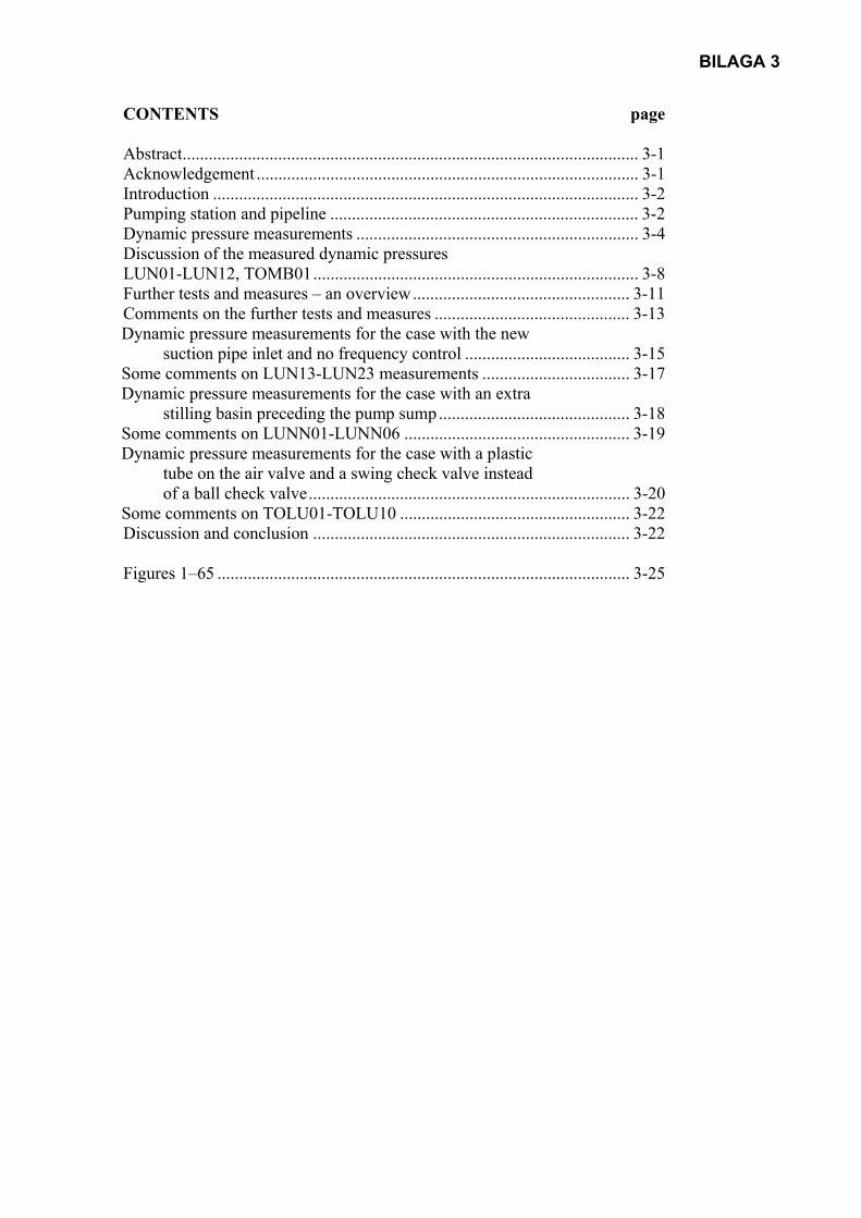
BILAGA 3

CONTENTS page Abstract......................................................................................................... 3-1 Acknowledgement ........................................................................................ 3-1 Introduction .................................................................................................. 3-2 Pumping station and pipeline ....................................................................... 3-2 Dynamic pressure measurements ................................................................. 3-4 Discussion of the measured dynamic pressures LUN01-LUN12, TOMB01........................................................................... 3-8 Further tests and measures – an overview.................................................. 3-11 Comments on the further tests and measures ............................................. 3-13 Dynamic pressure measurements for the case with the new

suction pipe inlet and no frequency control ...................................... 3-15 Some comments on LUN13-LUN23 measurements .................................. 3-17 Dynamic pressure measurements for the case with an extra

stilling basin preceding the pump sump............................................ 3-18 Some comments on LUNN01-LUNN06 .................................................... 3-19 Dynamic pressure measurements for the case with a plastic

tube on the air valve and a swing check valve instead of a ball check valve.......................................................................... 3-20

Some comments on TOLU01-TOLU10 ..................................................... 3-22 Discussion and conclusion ......................................................................... 3-22 Figures 1–65 ............................................................................................... 3-25

BILAGA 3

3-1

ABSTRACT The new Lunnarp pumping station receives wastewater from a food industry for conveyance to a treatment plant via further pumping stations. The pumping station, equipped with two self-evacuating centrifugal pumps with a suction head of 2–3 m, has experienced problems ever since the start-up of it. These problems manifested themselves on the suction and pressure sides of the pump for each of the pumps in the station. Pressure fluctuations could amount to 10–20 m H2O on the pressure side and 5–10 m H2O on the suction side, depending on the flow rate. Moreover, pump operation was accompanied by strong noise and vibrations, the former similar to cavitation sound. In order to try to find out the reason for the abnormal behaviour of the pumps, high frequency, dynamic pressure measurements were performed. The results from these measurements in conjunction with some other tests, observations and possible remedies are discussed in this report.

Ordinary vapour cavitation due to the suction head was ruled out as the cause of the problems. Instead, a number of other hypotheses were put forward; resonance due to the frequency control system, physical damage of the impellers, bad design of the suction pipe and/or the pump sump, gas/air bubbles in the sewage water, malfunctioning air valve in the pump itself, the downstream pipeline. Transient pressure measurements and/or visual observations were performed considering these hypotheses and for different pump operations and it was concluded that the pump problem was related to the existence of air/gas bubbles in the pump, although they were seemingly not related to the pump sump, the wastewater or the suction pipe. The measurements revealed that pressure fluctuations occurred more or less for all motor frequencies 0–50 Hz but especially strong and very regular high frequency pressure fluctuations were observed for motor frequencies about 38–40 Hz. An interesting finding was that a rough estimate of the resonance frequency (44 Hz) of the air valve agreed well with the above-mentioned range 38–40 Hz. Connecting the air valve to the pump sump with a small plastic tube proved to be partly successful as the pressure fluctuations on the suction side disappeared more or less entirely.

The final conclusion was that the cause of the pump problems was not fully determined. It seemed, however, that part of the explanation was related to the existence of air/gas in the pump. The source of the air/gas is not fully understood but there are several indications that air entrainment is related to the operation of the air valve.

ACKNOWLEDGEMENT

This report has been elaborated within the scope of a research project on ”Problems and beneficial use of hydraulic transients” supported by Ångpanneföreningens Forskningsstiftelse and VA-Forsk. This support is gratefully acknowledged.

BILAGA 3

3-2

INTRODUCTION The Lunnarp pumping station is located in the municipality of Tomelilla, Skåne. The station is one in a series of pumping stations conveying wastewater, mainly from the Skåne Mejerier food processing plant, to the wastewater treatment plant in the small town of Tomelilla. The Skåne Mejerier plant produces juices and milk-based products generating large amounts of wastewater with very high contents of BOD7, of the order of 1,000 mg O2/l. The nature of the wastewater implies that it is absolutely forbidden for environmental reasons to discharge it untreated – even occasionally – into local water courses. Moreover, the food processing plant is in operation more or less continuously 24h a day, thus delivering a steady flow of wastewater, which has to be taken care of in the municipal wastewater treatment plant. Thus, it is of utmost importance that the pumping stations for the conveyance of the wastewater from the food processing plant to the wastewater treatment plant are absolutely reliable. The pumping station in Lunnarp has been considered less reliable due, among other things, to its age and to corrosion problems. A new pumping station has thus very recently been built in the immediate neighbourhood of the old one in order to replace it while using the same pipelines. The new pumping station is equipped with two self-evacuating centrifugal pumps in parallel with a suction head of about 2–3 m. The pumps are of the variable speed type with the motor frequency controlled by the water level in the pump sump. Operation of the pumps revealed a serious problem – i.e. a strong, cavitation-like sound was generated somewhere in the pumps during operation and at the same time an ordinary manometer installed on the pressure side of the pumps displayed a seemingly very unsteady water pressure. Obviously, the pumps did not work properly and moreover, there was a fear that the pumps should wear out quickly and/or stop functioning suddenly, which would be devastating considering the importance of the pumping station. The immediate hypothesis as to the cause of the problems was that cavitation occurred in the pump due to too low pressures on the suction side of the pump, possibly due to an improper design of the suction pipe. In order to try to find out the reason for the abnormal behaviour of the pumps, high frequency, dynamic pressure measurements were performed. The results from these measurements in conjunction with some other tests, observations and possible remedies will be discussed in this report. PUMPING STATION AND PIPELINE The new pumping station is connected to the existing pipeline from the old pumping station via a 14 m long PEH pipe, diameter 150 mm. The old pumping station – with a check valve on the pressure side – is located 4 m upstream of the above-mentioned junction. From the junction pressurized flow takes place in a ductile iron pipe, diameter 150 mm, up to a well from which the further transport takes place by gravity. The length of the ductile iron pipeline is 750 m. The profile is shown in Fig 1 and the location of the two pumping stations in Fig 1a. The geometric head is thus about 9 m. The outline of the pumping station is shown in Figs 2a,b,c and a photo of the pumping station is shown in Fig 3. The incoming wastewater enters the circular pump sump, diameter 2.5 m, at the bottom of the sump, see Figs 2a,b. The station is equipped with two self-evacuating pumps in parallel, located some 2–3 meters above the sump water level. One possible cause of the pumping problems was assumed to be related to the suction pipe

BILAGA 3

3-3

and this part will be described in some detail. Originally, the suction pipe was assumed to be too small and thus a modification of the inlet part was carried out, Fig 4. However, this change did not improve the operational performance of the pumps. The original pressure transient measurements (LUN01–LUN12) described in this report will thus refer to the conditions after the suction pipe modification according to Fig 4. The inlet part of the suction pipe (pipes) in Figs 2a,b should thus be substituted with the configuration shown in Fig 4. The following measures apply: pipe entrance to suction side of the pump: + 64.50 m bottom level of the pump sump: + 60.60 m entrance level to the suction pipe: + 60.80 m Each suction pipe had the following design, starting at the pump sump entrance:

- a Φ 150 mm pipe, 300 mm long, with no special precaution for smooth inflow (i.e. just a cut-off pipe), see also Fig 4

- a conical transfer, 100 mm long, from the Φ150 mm pipe to a Φ100 mm long pipe, see also Fig 4

- a Φ100 mm pipe up to the suction side of the pump. This Φ100 mm pipe (about 4 m long) also had two 450 elbows and three 900 elbows, the latter ones located just some dm:s upstream the pump, Fig 3.

The design on the pressure side of the pumps was as follows. Each branch of the piping after the pumps was equipped with a ball check valve and after the junction of the two branches the common pipe had a shut-off valve as well. Moreover, a few meters downstream of the latter valve a short connection via a Φ25 mm pipe existed to an air vessel, total volume 0.120 m3, with unknown air volume, see Fig 5. At the highest point of the pipeline, just after the junction, a small ball valve was fitted in order to let out possible trapped air, Fig 6. The two pumps were of the make Gormann Rupp, self-evacuating centrifugal pumps, type T4A3-B, see Fig 7. This type of pump can be located rather high above the pump sump water level – i.e. sub-atmospheric pressure will prevail in the suction pipe during operation and also at standstill due to the existence of a ball check valve at the entrance to the pump on the suction side, see Fig 7. Start of a pump can take place with the pump casing only partly filled with water and a completely empty (of water) suction pipe. A kind of an air valve (type GRP 33-07) is located on the pressure side of the pump, incorporated with the pump casing itself, Figs 8,9. The purpose of the valve is to discharge air at pump start from the pump itself and/or from the possibly empty suction pipe. The valve consists essentially of a horizontal, spring-loaded axis (piston) which, at one end (to the right in Fig 9), is attached to a membrane. The axis can move back and forth depending on the balance between the spring force and the pressure on the membrane. If the axis moves to the left, the outlet from the valve is closed, whereas a right-hand position of the axis means that there is a connection between the interior of the pump and the atmosphere. With air in the pump the pressure (due mostly to air) on the membrane is too low for counteracting the spring force – thus the valve stays open letting out air (or air/water mixture) at pump start. With no air in the pump during pump operation the water pressure on the membrane rises due to increased losses in the small “channel” for the conveyance of water to the outlet (bottom of the valve in Fig 9). This

BILAGA 3

3-4

increased membrane pressure force surpasses the spring force and the axis moves to the left, closing the valve. The pumps were of the variable speed kind which was accomplished by controlling the frequency of the motor voltage. This meant that the pump speed was proportional to the motor voltage frequency with the voltage frequency of 50 Hz corresponding to a rotational speed of 1,550 rpm for the pump. The motor was attached to the pump in such a way (with a belt) that full motor speed of 1,450 rpm corresponded to a pump speed of 1,550 rpm. The pump speed was controlled by the water level in the pump sump – i.e. the normal operation of the pumps should be to keep the water level in the sump constant by setting a certain, desired value of the sump level for the frequency control system. This level was chosen to be about sump level = 0.75 m which can be translated into a distance from the sump level to the suction entrance of the pump according to the following relation: ∆z = - sump level + 3.86 m (1)

where ∆z = distance from the suction side of the pump to the water level of the pump sump.

This means that the distance ∆znorm from the water level to the suction side of the pump for normal operation is: ∆znorm = 3.11 m (2) The corresponding distance between the water level of the sump and the intake end of the suction pipe is 0.56 m. The pump curve is shown in Fig 10, which gives for 1,550 r/m:

Qr = 0.025 m3/s, i.e. 90 m3/h Hr = 19.0 m H2O

DYNAMIC PRESSURE MEASUREMENTS Two dynamic pressure transducers from Transamerica Instruments Ltd, Basingstoke, England, based on pressure sensitive resistances in part of a Wheatstone bridge, and capable of measuring sub-atmospheric pressures (down to vacuum), were used for the measurements:

Type BHL-4241-00, range 0–10 bar Type BHL-4241-00, range 0–25 bar

The upper frequency limit of the transducers is about 25 kHz. The transducers have been calibrated against different, known pressures showing a completely linear relationship between pressure and output voltage as well as very stable calibration characteristics – see Fig 11 for the 25 bar calibration curve. Moreover, the transducers were checked against the atmospheric pressure on site, thus making it possible (if

BILAGA 3

3-5

necessary) to perform some small modification to the standard calibration curves. The measurement error was assessed to be 0.1–0.2 m H2O. The two pressure transducers were attached to the suction and pressure sides of the pump respectively via small ball valves, Fig 12. On the suction side the transducer was located immediately upstream of the check valve belonging to the pump itself. On the pressure side the transducer was located downstream of the pump impeller but immediately upstream of the check valve in the pipeline. This meant that – at pump stop and closure of the downstream check valve – the latter transducer did not respond to the flow conditions in the pressure side of the pipeline. The pressure measurements were controlled via an ABC80 computer and a very stable amplifier. There are primarily three reasons for using this rather old computer:

- existing software - accuracy, as the A/D conversion card matches the transducers in a very

suitable way - the proven robustness of the system.

The sampling rate of the dynamic pressure measurements was maximum 640 Hz using one transducer only and 50 Hz using two transducers simultaneously. Pressure data was transferred to diagrams using LOTUS 1-2-3 software. The following pressure measurements were performed initially (the electromagnetic flow meter did not work during these measurements). LUN01, Figs 13,14 One transducer at the suction side. One pump (left one) running with motor voltage frequency 38.7 Hz, corresponding to 1,197 rpm for the pump. Pump sump level 0.75 m, i.e. ∆z=3.11 m. Sampling frequency 640 Hz, sampling time 5 s. It was unknown if the old pumping station was operating. Fig 13 shows the entire pressure record and Fig 14 a blow-up of the pressure variations during 0.7 s. LUN02, Figs 15,16 One transducer at the suction side. One pump (left one) running with motor voltage frequency 50 Hz, corresponding to 1,550 rpm for the pump. Pump sump level 0.95 m, i.e. ∆z=2.91 m. Sampling frequency 640 Hz, sampling time 5 s. The old pumping station was in operation. Fig 15 shows the entire pressure record and Fig 16 a blow-up of the pressure variations during 0.7 s.

BILAGA 3

3-6

LUN03, Figs 17,18,19 One transducer on the suction side. One pump (left one) running with motor voltage frequency 50 Hz corresponding to 1,550 rpm for the pump. Pump sump level 0.95 m, i.e. ∆z = 2.91 m. Sampling frequency 640 Hz, sampling time 5 s. The old pumping station was at standstill. Fig 17 shows the entire pressure record, Fig 18 a blow-up of the pressure variation during 1.5 s and Fig 19 a blow-up of the pressure variations during 0.7 s. LUN04, Fig 20,21 One transducer on the suction side. One pump (left one) running with motor voltage frequency 37.8 Hz corresponding to 1,171 rpm for the pump. Pump sump level 0.73 m, i.e. ∆z = 3.13 m. Sampling frequency 640 Hz, sampling time 5 s. The old pumping station was at standstill. Fig 20 shows the entire pressure record and Fig 21 a blow-up of the pressure variation during 0.7 s. LUN06, Fig 22 One transducer on the pressure side. One pump (left one) running with motor voltage frequency 40 Hz corresponding to 1,240 rpm for the pump. Pump sump level 0.75 m, i.e. ∆z = 3.11 m. Sampling frequency 50 Hz, sampling time 30 s. The old pumping station was at standstill. Fig 22 shows the entire pressure record. LUN07, Fig 23 One transducer at the pressure side. Start one pump (left one) from motor voltage frequency 0–50 Hz corresponding to full speed 1,550 rpm for the pump. Pump sump level 0.99 m, i.e. ∆z = 2.87 m. Sampling frequency 50 Hz, sampling time 60 s. Old pumping station in operation. Fig 23 shows the entire pressure record. LUN08, Fig 24 One transducer on the pressure side. Start one pump (left one) from motor voltage frequency 0–50 Hz corresponding to full speed 1,550 rpm for the pump. Pump sump level 0.99 m, i.e. ∆z = 2.87 m. Sampling frequency 50 Hz, sampling time 60 s. Old pumping station at standstill.

BILAGA 3

3-7

Fig 24 shows the entire pressure record. LUN09, Fig 25 One transducer on the pressure side. Stop one pump (left one) from motor voltage frequency 50–0 Hz. Pump sump level (not recorded). Sampling frequency 50 Hz, sampling time 30 s. Old pumping station at standstill. Fig 25 shows the entire pressure record. LUN10, Fig 26 Two transducers, one on the suction side and one on the pressure side. Stop one pump (left one) from motor voltage frequency 50–0 Hz. Pump sump level 0.84 m, i.e. ∆z = 3.02 m. Sampling frequency 50 Hz, sampling time 30s. Old pumping station at standstill. Fig 26 shows the entire pressure records. LUN11, Fig 27 Two transducers, one on the suction side and one on the pressure side. Start one pump (left one) from motor voltage frequency 0–50 Hz corresponding to full speed 1,550 rpm for the pump. Pump sump level 1.54 m, i.e. ∆z = 2.32 m. Sampling frequency 50 Hz, sampling time 30 s. Old pumping station at standstill. Fig 27 shows the entire pressure record. LUN12, Fig 28 Two transducers, one on the suction side and one on the pressure side. One pump (left one) running with motor voltage frequency 50 Hz corresponding to 1,550 rpm for the pump. Pump sump level 1.30 m, i.e. ∆z = 2.56 m. Sampling frequency 50 Hz, sampling time 20 s. Fig 28 shows the entire pressure record. TOMB01, Fig 29 For the purpose of comparison a dynamic pressure measurement was done at the next downstream pumping station. This station was equipped with exactly the same pumps and with the same type of air valve (the spring properties might be different). Moreover, the suction head was more or less the same as for the Lunnarp pumping station. The pressure measurement was performed on the suction side of one of the pumps for the case with the pump running with a motor voltage frequency of 33 Hz and with the pump sump level at 0.49 m, i.e. ∆z = 2.62 m. Sampling frequency 50 Hz, sampling time 20 s. Fig 29 shows the entire pressure record.

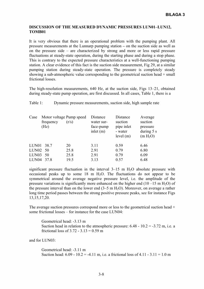
BILAGA 3

3-8

DISCUSSION OF THE MEASURED DYNAMIC PRESSURES LUN01–LUN12, TOMB01 It is very obvious that there is an operational problem with the pumping plant. All pressure measurements at the Lunnarp pumping station – on the suction side as well as on the pressure side – are characterized by strong and more or less rapid pressure fluctuations at steady-state operation, during the starting phase and during a stop phase. This is contrary to the expected pressure characteristics at a well-functioning pumping station. A clear evidence of this fact is the suction side measurement, Fig 29, at a similar pumping station during steady-state operation. The pressure is completely steady showing a sub-atmospheric value corresponding to the geometrical suction head + small frictional losses. The high-resolution measurements, 640 Hz, at the suction side, Figs 13–21, obtained during steady-state pump operation, are first discussed. In all cases, Table 1, there is a Table 1: Dynamic pressure measurements, suction side, high sample rate Case Motor voltage Pump speed Distance Distance Average frequency (r/s) water sur- suction suction (Hz) face-pump pipe inlet pressure inlet (m) - water during 5 s level (m) (m H2O) LUN01 38.7 20 3.11 0.59 6.46 LUN02 50 25.8 2.91 0.79 6.80 LUN03 50 25.8 2.91 0.79 6.09 LUN04 37.8 19.5 3.13 0.57 6.48 significant pressure fluctuation in the interval 3–15 m H2O absolute pressure with occasional peaks up to some 18 m H2O. The fluctuations do not appear to be symmetrical around the average negative pressure level, i.e. the amplitude of the pressure variations is significantly more enhanced on the higher end (10 –15 m H2O) of the pressure interval than on the lower end (3–5 m H2O). Moreover, on average a rather long time period passes between the strong positive pressure peaks, see for instance Figs 13,15,17,20. The average suction pressures correspond more or less to the geometrical suction head + some frictional losses – for instance for the case LUN04: Geometrical head: -3.13 m

Suction head in relation to the atmospheric pressure: 6.48 - 10.2 = -3.72 m, i.e. a frictional loss of 3.72 - 3.13 = 0.59 m

and for LUN03: Geometrical head: -3.11 m

Suction head: 6.09 - 10.2 = -4.11 m, i.e. a frictional loss of 4.11 - 3.11 = 1.0 m

BILAGA 3

3-9

These measured average suction heads and frictional losses seem to be quite reasonable, especially considering that the motor speed in case LUN03 is 1,450 rpm and in case LUN04 1,122 rpm implying a lower pump flow in the latter case and thus lower frictional losses. As the pump flow is proportional to the motor speed and frictional losses are proportional to the flow squared, one gets:

29.1122,1450,1

QQ

122,1

450,1 ==

67.129.1lossloss 2

122,1

450,1 ==

Measured loss rate: 69.159.00.1

= , i.e. a very good agreement between loss ratios

estimated in these two ways. The measured, temporal average suction pressure heads of the order of 6–6.50 m H2O corresponding to an absolute energy head, including the velocity head at the pump inlet of about 0.5 m H2O (diam 100 mm and Q = 0.025 m3/s), of 6.50–7.0 m H2O should be compared to the required NPSH value (Net Positive Suction Head) for the pumps, see the pump curve, Fig 10. The minimum NPSH value according to the manufacturer is of the order of 1–3 m H2O, which is considerably below the measured average operational total suction head. Thus, one should not expect any cavitation problems due to too low suction pressures. An enhancement of the pressure records shows some very interesting facts, Figs 14, 16, 19, 21. The two cases with motor voltage frequency 37.8 (Fig 21) and 38.7 Hz (Fig 14) respectively display a very regular, oscillatory behaviour of the suction pressure with oscillating frequencies of 38.9 Hz and 40.5 Hz respectively, i.e. related (about equal) to the motor voltage frequencies. However, the two cases with 50 Hz motor voltage frequency, Fig 16 and Fig 19, do not display the same regular, oscillatory behaviour – the oscillations are less regular with an average frequency of about 36–38 Hz which is considerably lower than the motor voltage frequency. The rest of the transient measurements, LUN06–LUN12, were carried out with a sampling frequency of 50 Hz. This means that the amplitude characteristics of the pressure oscillations were described well whereas an erroneous description of the high frequency characteristics could occur due to the aliasing phenomenon (the sampling rate should be at least twice the maximum oscillatory frequency). For this reason no enhancements of these pressure recordings are shown/discussed. The measurement of the pressure at the pressure side with one pump running and a motor voltage frequency of 40 Hz, Fig 22, shows qualitatively the same unsteady behaviour with pressure variations in the interval 15–25 m H2O with occasional pressure peaks reaching 28 m H2O. The start-up sequence with pressure measurement on the pressure side, 0–50 Hz motor voltage frequency, in Fig 23 shows that the pressure initially is atmospheric. As the flow starts building up, the pressure increases and the amplitude of the pressure oscillations starts increasing from the very start. When the motor voltage 50 Hz has been reached

BILAGA 3

3-10

the unsteady pressure characteristics seem to stabilize in a statistical sense with fluctuations in the interval 22–45 m H2O with occasional, significantly higher peaks. The start-up sequence in Fig 24 is very similar to the one in Fig 23 except that in this case the old pumping station was at standstill. The pressure characteristics are also very similar to the one in Fig 23 although with somewhat smaller pressure fluctuations. The pump tripping sequence (motor voltage frequency 50–0 Hz) in Fig 25 with the pressure measurement on the pressure side shows that the pressure rapidly decreases to the atmospheric one and stays at this latter level as the air valve in the pump opens when the pressure in the pump tends to go sub-atmospheric. The amplitude of the pressure fluctuations decreases with decreasing motor voltage frequency. The simultaneous measurements at both the pressure and the suction side respectively at a pump trip occasion in Fig 26 indicate that the unsteady oscillations occur at both locations at the same time. It is, however, difficult to find any correlation – at least from a visual inspection – between a pressure disturbance on the suction side with the one on the pressure side. The simultaneous measurement of pressures at the suction and pressure side respectively in Fig 27 at a pump start does, however, show an interesting feature. On the suction side pressure disturbances seem to appear and to increase in amplitude at the very start of the pump. At the pressure side, however, pressure builds up initially without any significant disturbances until the pressure has reached about 15 m H2O (absolute pressure). At this point in time the pressure disturbances start to grow significantly. The reason for this phenomenon is not known – one hypothesis could be that the check valve on the pressure side does not open until the geometric head is surpassed. Another hypothesis could be that the air valve does not open until the pressure is 15 m H2O. Fig 28, with simultaneous suction and pressure side measurements for a “steady state” running pump, does not show any visual correlation between the pressure disturbances at the two locations. Finally, table 2 shows the data for LUN6–LUN12 concerning ∆z = distance from the suction side of the pump to the water level and ∆x = distance from the pump sump water level to the intake of the suction pipe. Table 2: Pump sump level data Measurement ∆z ∆x

(m) (m) LUN05 2.93 0.74 LUN06 3.11 0.56 LUN07 2.87 0.80 LUN08 2.81 0.86 LUN09 - - LUN10 3.02 0.65 LUN11 2.32 1.35 LUN12 2.56 1.11

BILAGA 3

3-11

Tables 1 and 2 show that most of the investigated cases are favourable as compared to the design ∆znorm = 3.11 m situation, i.e. the geometrical suction head is smaller and the distance from the water surface to the suction pipe intake is larger. The pressure measurements for all these cases show that the pump problem prevails. Moreover, the design case, ∆z = 3.11 m, LUN06, has also got the pressure pulse problem. It should also be mentioned that visual inspection of the pump sump did not indicate any existence of vortices in the pump sump. All the initial pressure measurements, LUN01–LUN12, indicated that more or less severe, unsteady pressures occurred both at the suction and pressure side respectively during start-up, tripping and steady state operation of the pumps. The cause of the problem could, however, not be deduced unambiguously. In the first place one should emphasize that there were no indications that the unsteady pressure problem was related to ordinary transient pressures in the 750 m long pipeline. Assuming a wave propagation velocity in the PEH pipe of the order of 400 m/s gives an oscillation period T = 7.5 s, i.e. a frequency of 0.13 Hz which is far too low compared to the observed unsteady pressure frequencies. Moreover, tests were performed with a valve closed immediately downstream of the pump, i.e. no flow from the pump, which did not alleviate the problem. A few observations and possible conclusions should be mentioned at this stage:

- ordinary vapor cavitation due to too low suction head does not seem to be a reason. The suction head is only of the order of -2–(-3) m H2O when disturbances start to occur whereas NPSH is considerably lower

- the disturbances seem to change character depending on the motor voltage frequency. It was found that the oscillations were very regular (almost sinusoidal) at a frequency of about 38–40 Hz whereas a higher frequency, 50 Hz, caused the disturbances to be much more irregular. Moreover, at the motor voltage frequency 38–40 Hz the pressure disturbances had approximately the same frequency as the motor voltage whereas the pressure oscillating frequency differed significantly from the motor voltage frequency when the latter was 50 Hz

- the level variations in the pump sump did not seem to have any significant effect on the problems.

FURTHER TESTS AND MEASURES – AN OVERVIEW In order to try to understand the cause of the unsteady pressures a “trial and error” process of tests, modifications, observations was initiated, some of them complemented with pressure transient measurements but in several cases just relying on visual and/or audible results.

BILAGA 3

3-12

The main (1) hypothesis for the pump problems was based on an assumption that these were related to the existence of gas/air in the pump system. Several sources/mechanisms for this occurrence were suggested:

- the nature of the sewage water, possibly containing significant amounts of bubbles and/or dissolved gas

- the design of the suction pipe which might enhance the release of air or promote the entrainment of air from existing bubbles or from vortices in the pump sump

- the functioning of the air release valve on the pressure side of the pump. There were also other hypotheses put forward: 2. Some kind of resonance phenomenon linked to the frequency control system of

the motor voltage implying that small disturbances were amplified. 3. Some deficiency with the pump (pumps) itself (themselves), for instance

concerning the impeller. The air/gas hypothesis led to a number of studies:

- the use of a 150 mm diameter PEH suction pipe without any bends but with no special precaution (just a cut-off of the pipe) at the pipe inlet

- a change of the design of the inlet of the original suction pipe, i.e. using a conical entrance with the inlet diameter 300 mm, Fig 2a

- testing a case with a very high water surface in the pump sump in order to check if air was sucked into the suction pipe through vortex formation

- filling the pump sump with wastewater and letting it stay there for a while before starting the pump in order to make sure that possible bubbles escaped from the pump sump before pumping

- filling the pump sump with ordinary tap water, thus minimizing the amount of dissolved gases and existence of bubbles

- construction of a “stilling well”, 2 m in diameter, preceding the ordinary pump sump, thus enhancing the gas release from the wastewater

- checking the functioning of the air valve and connecting it via a tube to the pump sump water, thereby avoiding the sucking-in of air during possible sub-atmospheric phases during pump operation.

The second hypothesis related to resonance due to some kind of possible feedback in the frequency control system was studied by disconnecting this system and instead using an external, constant-frequency (50 Hz) voltage supply. The third hypothesis related to the pump itself was addressed by inspection of the interior of the pump (impeller etc).

BILAGA 3

3-13

COMMENTS ON THE FURTHER TESTS AND MEASURES The different points described in the above chapter will be discussed briefly as to the effect on the unsteady pressure problem. It should be emphasized already here that the problem was not solved completely although it was possible to reduce the noise level and the pressure oscillations significantly. A number of dynamic pressure measurements in conjunction with some of the measures will also be presented and discussed:

• the provisional, straight PEH pipe did not make any difference to the problem (judging from the noise level)

• the use of a modified inlet part (cone with the diameter 300 mm) did not improve the performance of the pump to any noticeable extent. This cone was kept for the rest of the tests discussed here

• a test with the pressure side valve closed, i.e. with the pump running but with no flow through it, was performed (LUN18). No significant improvement was found

• a special test was carried out with a very high water level in the pump sump, corresponding to a distance of 1.11 m from the water level to the suction pipe inlet. In this way vortex generation should be avoided in the pump sump, see Fig 30, i.e. a head of 3.5 ft (about 1.11 m) and a velocity of about 3.5 ft/s (about 1.1 m/s) is well below the limit for vortex problems. No improvement of the noise and the unsteady pressure problems was found. It should be added that in several cases with lower pump levels the pump sump was visually inspected for the possible existence of vortices. No such a vortex was ever discovered

• small amounts of air were let into the suction side of the pump via the valve at the point for pressure measurements on the suction side of the pump. No improvement in the pressure fluctuations on the pressure side could be noticed. Increasing the amount of air through the valve diminished the water flow by half (from 43 m3/h to 20 m3/h) and did also decrease the amplitude of the pressure fluctuations on the pressure side significantly. This latter effect was most probably due to the decreased flow velocity

• the test with a certain amount of wastewater left for an extended time in the pump sump before pumping did not show any improvement in the pump sump. The same conclusion was drawn from the test with ordinary tap water in the pump sump (judging from the noise level)

• the extra 2.0 m diameter stilling well did not improve the pump operation • the air valve behaviour during a start of a pump was observed and it was found

that there was no observable valve oscillation , i.e. the valve seemed to stay in its closed position after a short while. The reason for this point was a suspicion that the piston arrangement of the valve might have a resonance frequency of the same order as the impeller rotation. The former could be estimated in a rough way as follows, Fig 31. The valve basically consists of a piston, a spring and a membrane. Differential pressure across the membrane exerts a force on the spring and thus on the piston which can move back and forth in the x-direction. The movement of the piston is described by (no friction):

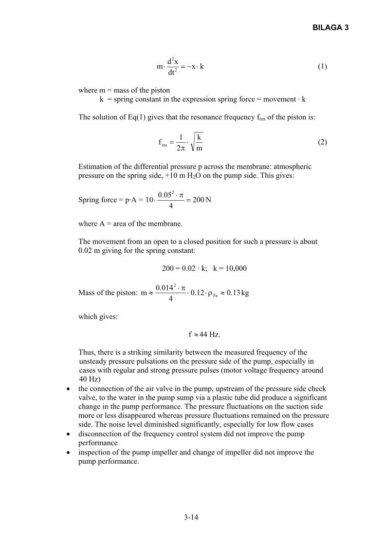
BILAGA 3

3-14

kxdt

xdm 2

2

⋅−=⋅ (1)

where m = mass of the piston k = spring constant in the expression spring force = movement · k The solution of Eq(1) gives that the resonance frequency fres of the piston is:

mk

21fres ⋅π

= (2)

Estimation of the differential pressure p across the membrane: atmospheric pressure on the spring side, +10 m H2O on the pump side. This gives:

Spring force = p·A = N2004

05.0102

=π⋅

⋅

where A = area of the membrane. The movement from an open to a closed position for such a pressure is about 0.02 m giving for the spring constant:

200 = 0.02 · k; k = 10,000

Mass of the piston: kg13.012.04

014.0m Fe

2

≈ρ⋅⋅π⋅

≈

which gives:

f ≈44 Hz.

Thus, there is a striking similarity between the measured frequency of the unsteady pressure pulsations on the pressure side of the pump, especially in cases with regular and strong pressure pulses (motor voltage frequency around 40 Hz)

• the connection of the air valve in the pump, upstream of the pressure side check valve, to the water in the pump sump via a plastic tube did produce a significant change in the pump performance. The pressure fluctuations on the suction side more or less disappeared whereas pressure fluctuations remained on the pressure side. The noise level diminished significantly, especially for low flow cases

• disconnection of the frequency control system did not improve the pump performance

• inspection of the pump impeller and change of impeller did not improve the pump performance.

BILAGA 3

3-15

DYNAMIC PRESSURE MEASUREMENTS FOR THE CASE WITH THE NEW SUCTION PIPE INLET AND NO FREQUENCY CONTROL

A number of measurements were performed with the new design of suction pipe inlet, Fig 2b, and with the frequency control system disconnected. The latter implied the use of a constant motor voltage frequency of 50 Hz supplied from a mobile generator. The old pumping station was disconnected in all cases. In some cases pressure measurements were performed on the pressure side downstream of the second check valve at the pump. This measurement point refers to a location on the common pipe leading from the two pumps, Fig 3, and is visible in the upper left hand corner of the figure on the topmost, horizontal pipeline. The measurement point is located 0.95 m above the pump inlet level.

LUN13, Figs 32,33,34 One transducer on the suction side. Start one pump (left one) No frequency control Pump sump level 1.07 m, i.e. ∆z = 2.80 m Sampling frequency 50 Hz, sampling time 50 s Fig 32 shows the entire pressure record, Fig 33 a blow-up of the start period and Fig 34 a blow-up of the steady state operation.

LUN14, Fig 35 One transducer on the suction side One pump (right one) running Downstream valve closed (Qpipe=0). This valve is located immediately downstream the pump and thus the pressure vessel was not active

No frequency control Pump sump level 0.95 m, i.e. ∆z = 2.92 m Sampling frequency 640 Hz, sampling time 5s Fig 35 shows the entire pressure record LUN15, Figs 36,37,38 One transducer on the suction side Start one pump (right one) No frequency control Pressure vessel connected Flow Qpipe = 67 m3/h Pump sump level 1.32 m, i.e. ∆z = 2.55 m Sampling frequency 50 Hz, sampling time 50 s Fig 36 shows the entire pressure record, Fig 37 a blow-up of the initial phase and Fig 38 a blow-up of the steady state phase

LUN16, Figs 39,40 Two transducers, one on the suction side and one on the pressure side Start one pump

BILAGA 3

3-16

No frequency control Flow Qpipe = 70 m3/h Sampling frequency 50 Hz, sampling time 50 s Pump sump level 1.53 m, i.e. ∆z = 2.34 m. Fig 39 shows the entire pressure record, Fig 40 a blow-up of the steady state phase LUN17, Fig 41 One transducer on the suction side One pump (left one) running Frequency control, 50 Hz Flow Qpipe = 66 m3/h Sampling frequency 640 Hz, sampling time 5 s Pump sump level unknown Fig 41 shows the entire pressure record LUN18, Fig 42 One transducer on the suction side One pump (left one) running Frequency control Flow Qpipe = 0, i.e. the downstream valve was closed Sampling frequency 640 Hz, sampling time 5 s Pump sump level 1.06 m, i.e. ∆z = 2.81 m Fig 42 shows the entire pressure record LUN19, Fig 43 Two pressure transducers, one on the suction side and one on the pressure side Start one pump (left one) Frequency control 0–50 Hz Flow Qpipe = 66 m3/h Sampling frequency 50 Hz, sampling time 50 s Pump sump level 0.99 m, i.e. ∆z = 2.88 m Fig 43 shows the entire pressure record LUN20, Fig 44 Two pressure transducers, one on the suction side and one on the pressure side Start one pump (left one) Frequency control 0–50 Hz Flow Qpipe = 64 m3/s Aeration of the pressure side of the pump before start Sampling frequency 50 Hz, sampling time 50 s Pump sump level 0.95 m, i.e. ∆z = 2.92 m Fig 44 shows the entire pressure record LUN22, Figs 45,46 One transducer on the pressure side

BILAGA 3

3-17

One pump (left one) running Frequency control (40 Hz) Flow Qpipe = 43 m3/s Sustained inlet of some air through the point for pressure measurements on the suction side (air intake controlled using a ball valve) Sampling frequency 640 Hz, sampling time 5 s Pump sump level0.80 m, i.e. ∆z = 3.07 m Fig 45 shows the entire pressure record and Fig 46 is a blow-up LUN23, Figs 47,48 The same conditions as for LUN22 except that the flow was Qpipe = 20 m3/s and more air was let in. Fig 47 shows the entire pressure record and Fig 48 a blow-up. SOME COMMENTS ON LUN13–LUN23 MEASUREMENTS

- All measurements with the frequency control system disconnected, LUN13–LUN16, show strong pressure pulsations on both the suction side and the pressure side. LUN16 (Figs 39,40) and LUN19 (Fig 43) are two rather similar cases from a measurement and operational point of view respectively except that LUN16 has no frequency control and LUN19 has got one. A visual comparison of the steady state oscillatory pressure amplitudes shows that they have approximately the same magnitude. Thus, the frequency control does not seem to affect this aspect of the pump problem. There is, however, a certain difference as to the nature of the pressure oscillations – the no-frequency control seems to be more regular (sinusoidal) than the frequency case, especially on the pressure side of the pump. There is also a marked difference during the start phase, which in the first place is considerably faster in the no-frequency case. Moreover, there is initially a very regular, relatively low frequency oscillation on the pressure side in the no-frequency control case, which is not visible at all in the frequency control case. Finally, one could notice, on the suction side for the frequency control case, the significant enhancement of the pressure disturbances during part of the start phase – corresponding to a certain motor frequency interval

- LUN14 (no-frequency control, Fig 35) and LUN18 (frequency control, Fig 42) could be compared for the no-flow case through the pump. Both cases experience relatively strong pressure fluctuations on the suction side, with the frequency control case having slightly less marked oscillations. These no-flow cases do of course also emphasize the fact that it is not the design of the suction pipe that causes the problems which instead seem to be related to the pump or the air valve themselves

- aeration of the pressure side of the pump before start has not affected the pressure oscillations, LUN20 (Fig 44)

- different amounts of steady air supply at the suction side of the pump will affect the pressure oscillations at the pressure side for otherwise equal operating conditions. Figs 45,46 show the case of a very small amount of air, seemingly not affecting the pressure pulsations significantly. One could notice the very regular oscillations, Fig 46, with a frequency of 43 Hz which

BILAGA 3

3-18

is very close to the motor frequency of 40 Hz. In this case the water flow was 43 m3/s.

Figs 47,48 show the case with a significantly higher air supply which has caused the

pressure oscillations to diminish considerably. Moreover, the pressure oscillations are less regular, Fig 48, but with the same frequency, 43 Hz, as for the low air supply case. The increased air supply has caused the water flow to diminish to 20 m3/s, which might explain the small amplitude of the pressure oscillations.

DYNAMIC PRESSURE MEASUREMENTS FOR THE CASE WITH AN EXTRA STILLING BASIN PRECEDING THE PUMP SUMP

A number of measurements were performed with the extra stilling basin (diameter 2 m) preceding the pump sump. The new design of the suction pipe was used. The frequency control system was in operation.

LUNN01, Fig 49 One transducer on the suction side Start one pump (left one) 0–45 Hz Pump sump level 1.30 m, i.e. ∆z = 2.57 m Flow Qpump = 79 m3/h Sampling frequency 50 Hz, sampling time 120 s Fig 49 shows the entire pressure record.

LUNN02, Fig 50

One transducer on the pressure side Start one pump (left one) 0–45 Hz Pump sump level 1.47 m, i.e. ∆z = 2.30 m Flow Qpump = 79.3 m3/h Sampling frequency 50 Hz, sampling time 120 s Fig 50 shows the entire pressure record

LUNN03, Fig 51

One transducer on the pressure side, downstream the check valve Stop one pump (left one) 45–0 Hz Pump sump level 1.28 m, i.e. ∆z = 2.59 m Flow Qpump = 79 m3/h Sampling frequency 50 Hz, sampling time 120 s Fig 51 shows the entire pressure record. LUNN04, Fig 52 One pressure transducer on the pressure side, downstream of the check valve Start one pump (left one) 0–45 Hz Pump sump level 1.46 m, i.e. ∆z = 2.41 m

BILAGA 3

3-19

Flow Qpump = 79 m3/h Sampling frequency 50 Hz, sampling time 120 s Fig 52 shows the entire pressure record. LUNN05, Fig 53 One pressure transducer on the pressure side Start one pump (right one) 0–45 Hz Pump sump level 1.21 m, i.e. ∆z = 2.66 m Flow Qpump = 77 m3/h Sampling frequency 50 Hz, sampling time 120 s Fig 53 shows the entire pressure record. LUNN06, Fig 54 One pressure transducer on the pressure side Start two pumps simultaneously Pump sump level 1.40 m, i.e. ∆z = 2.37 m Flow Qpipe = 89.7 m3/h Sampling frequency 50 Hz, sampling time 120 s Fig 54 shows the entire pressure record.

SOME COMMENTS ON LUNN01–LUNN06

- the measurement (LUNN01) on the suction side shows that fairly strong pressure fluctuations arise and persist at start and during steady state operation

- all measurements on the pressure side, upstream the second check valve, show that there are strong pressure fluctuations comprising 10–15 m H2O

- the measurement, LUNN04, on the pressure side, downstream the second check valve, shows a significantly diminished pressure fluctuation (3–5 m H2O). This fact should be compared with the measurement, LUNN02, corresponding to a more or less identical operation of the pump as far as flow, motor frequency, pump sump level are concerned. Thus, one gets the impression that the strong pressure fluctuations in the pump are a local phenomenon which attenuates rather quickly in the downstream (pressure side) direction of the pipeline

- the tripping situation in LUNN03 shows a slow pressure oscillation due to the effect of the pressure vessel

- a comparison between LUNN02 and LUNN05 shows that there is no difference between the left hand and the right hand pump as to the pressure fluctuations at start and during steady state operation

- start of two pumps simultaneously does not change the characteristics of the pressure fluctuations as compared to the start of one pump.

A general conclusion of these six measurements is that the extra stilling well has no effect on the pressure fluctuations.

BILAGA 3

3-20

DYNAMIC PRESSURE MEASUREMENTS FOR THE CASE WITH A PLASTIC TUBE ON THE AIR VALVE AND A SWING CHECK VALVE INSTEAD OF A BALL CHECK VALVE A number of measurements were performed with a plastic tube connected to the air valve and ending in the water in the pump sump. Moreover, the ball check valve on the suction side was changed to a swing check valve. These measurements represent the “final” situation in the pumping station – no further modifications have been done. The pumping station is thus working on an operational, long term basis now with the new suction pipe (300 mm cone), an extra stilling well, the plastic tube from the air valve and the new check valve. The noise level has diminished as well as the mechanical vibrations, and the pressure oscillations have diminished significantly on the suction side. The air vessel was disconnected in all cases.

TOLU01, Fig 55 One pressure transducer on the suction side Start one pump (left) 0–45 Hz (manual) Pump sump level 0.75 m, i.e. ∆z = 3.11 m Flow Qpump = 66.1 m3/h Sampling frequency 50 Hz, sampling time 60 s Fig 55 shows the entire pressure record TOLU02, Fig 56 One pressure transducer on the pressure side Start one pump, 0–45 Hz Pump sump level 0.75 m, i.e. ∆z = 3.11 m Flow ? Sampling frequency 50 Hz, sampling time 60 s Fig 56 shows the entire pressure record TOLU04, Fig 57 One pressure transducer on the pressure side Decreasing motor frequency, 46 Hz–33 Hz Pump sump level 0.80 m, i.e. ∆z = 3.06 m Flow at the end of the interval Qpump = 30 m3/h Sampling frequency 50 Hz, sampling time 60 s Fig 57 shows the entire pressure record TOLU05, Fig 58 One pressure transducer on the pressure side Stop one pump (left) 50 Hz–0 Hz Flow Qpump = 77 m3/h before the stop Pump sump level 0.80 m, i.e. ∆z = 3.06 m Sampling frequency 50 Hz, sampling time 60 s Fig 58 shows the entire pressure record

BILAGA 3

3-21

TOLU06, Fig 59 One pressure transducer on the pressure side downstream of the second check valve Stop one pump (right), 33 Hz–0 Hz Pump sump level 0.59 m, i.e. ∆z = 3.27 m Flow Qpump = 31.4 m3/h Sampling frequency 50 Hz, sampling time 60 s TOLU07, Fig 60 One pressure transducer on the pressure side downstream of the second check valve Stop two pumps simultaneously, 50 Hz–0 Hz Pump sump level 0.80 m, i.e. ∆z = 3.06 m Flow Qpump = 82.2 m3/h Sampling frequency 50 Hz, sampling time 10 s Fig 60 shows the entire pressure record TOLU08, Figs 61,62 One pressure transducer on the pressure side One pump (right) running, 36 Hz motor voltage frequency Pump sump level 0.61 m, i.e. ∆z = 3.25 m Flow Qpump = 44 m3/h Sampling frequency 640 Hz, sampling time 5 s Fig 61 shows the entire pressure record, Fig 62 a blow-up of part of the record. The frequency of the pressure fluctuations, Fig62, is 44 Hz TOLU09, Figs 63,64 One pressure transducer on the pressure side One pump (left) running, motor voltage frequency 50 Hz Pumps sump level 0.64 m, i.e. ∆z = 3.22 m Flow Qpump = 76 m3/h Sampling frequency 640 Hz, sampling time 5 s Fig 63 shows the entire pressure record, Fig 64 a blow-up of part of the record. The frequency of the pressure fluctuations, Fig 64, is 61 Hz TOLU10, Fig 65 One pressure transducer on the suction side One pump running, motor voltage frequency 50 Hz Flow Qpump = 76.7 m3/h Sampling frequency 640 Hz, sampling time 5 s Fig 65 shows the entire pressure record.

BILAGA 3

3-22

SOME COMMENTS ON TOLU01–TOLU10

- TOLU01, Fig 55, and TOLU10, Fig 65, show that the pressure fluctuations on the suction side have almost disappeared, even for high flows, 66–76 m3/h. This fact represents an important improvement in the pump operation

- on the pressure side there are still strong pressure fluctuations, see for instance TOLU05, Fig 58, where the pressure fluctuation span is up to 20 m H2O.

DISCUSSION AND CONCLUSION The new Lunnarp pumping station receives waste water from a food industry for conveyance to a treatment plant via further pumping stations. The pumping station has experienced problems ever since the start-up of it. These problems manifested themselves on the suction and pressure sides of the pump for each of the pumps in the station. Pressure fluctuations could amount to 10–20 m H2O on the pressure side and 5–10 m H2O on the suction side, depending on the flow rate. However, the pressure rarely passed below 5 m H2O (absolute pressure) on the suction side. Moreover, pump operation was accompanied by strong noise and vibrations, the former similar to cavitational sound. The pumps are self-evacuating, variable speed centrifugal pumps, equipped with a motor voltage frequency control system for the impeller rotation and thus the flow rate. The frequency and thus the flow rate are controlled by the pump sump level. Normally, the distance between the center of the pump intake and the pump sump water level is about 3 m. It was initially assumed that the pump problems could be attributed to cavitation due to the geometrical suction head and inappropriate design of the suction pipe and its inlet. A number of modifications of the suction pipe and tests with a high water level did not show any improvement as to the pump operation. Thus, a suction pipe without any 900 or 450 bends was tested as well as a suction pipe with a smoother inlet. Pressure measurements showed that problems (pressure fluctuations) started to appear at a suction pressure of about 7–8 m H2O (absolute pressure) and the average pressure stayed at about 6–7 m H2O (absolute pressure) during operation with a high flow rate (Qpump ~ 70–80 m3/h). This latter fact implies that friction in the suction pipe was not significant compared to the geometrical suction head. It was found that during a pump start-up situation pressure fluctuations started immediately on the suction side, whereas pulsations on the pressure side did not start to appear until the pressure had reached a certain level, about 14–16 m H2O (absolute pressure). This latter fact indicates a coincidence with the opening of the second check valve, i.e. the pump pressure starts to exceed the geometrical head in the 700 m long pressure pipeline. It was also found that the pressure oscillations on the suction side were very regular for pump motor frequencies of about 36–40 Hz whereas the highest motor voltage frequency, 50 Hz, produced considerably less regular oscillations. A similar phenomenon could be observed on the pressure side. The regular pressure pulsations looked, as if they were affected by air bubbles, i.e. with fairly sharp peaks but more rounded troughs. Subsequent tests with the introduction of small amounts of air on the suction side produced the same kind of pressure pulsations on the pressure side.

BILAGA 3

3-23

The amplitude of the pressure pulses seemed to depend on the flow rate to a certain degree, i.e. decreasing the flow rate did decrease the amplitudes. However, tests with zero flow rate (pumping against a closed downstream valve) did also produce significant pulsations, furthermore supporting the fact that it was not the nature of the flow in the suction pipe that caused the problems. As ordinary vapour cavitation was ruled out as the cause of the problems a few other hypotheses were put forward. First, two less likely ones are discussed very briefly, mainly in order to rule them out. The possible effect of the frequency control system in causing some kind of resonance phenomenon was investigated by disconnecting it and instead supplying the motor from a fixed 50 Hz electrical energy source. No improvement was found. Secondly, one could not exclude the possibility of the problem being related to the pump impeller. It was, however, less likely as both pumps showed the same behaviour. Inspection of the impellers did not disclose any visible damage. Thus, the main hypothesis remained that the problem was related to the existence of gas/air bubbles/pockets in the wastewater. Several possibilities of the air/gas source can be thought of – existing bubbles in the incoming flow, release of dissolved air/gas, introduction of air from vortices in the pump sump, air inlet through the air valve. A number of different measures/modifications in/of the pumping station and its operation were tested :

- high pump sump level, whereby the negative suction head diminished – less risk for the release of dissolved air/gas. Moreover, the risk for vortex generation and thus air inlet in the sump was avoided. No improvement - the use of ordinary tap water in the pump sump. No improvement - the use of an extra “stilling well” before the pump sump for making sure that possible, existing bubbles in the wastewater were released before pumping. No improvement.

These three points indicate that there are no bubbles in the wastewater entering the suction pipe intake. Moreover, no air inlet took place via vortices in the pump sump. The test with ordinary tap water indicates that the wastewater is not considerably more prone to gas release in the suction pipe due to the negative suction head. Tests with pumping against a closed downstream valve (i.e. no pump flow rate) showed significant pressure fluctuations on the suction side. Unfortunately, there were no measurements on the pressure side for the no-flow case. One could, however, study cases with simultaneous pressure measurements on both the suction and the pressure side respectively at pump start where the second (downstream) check valve obviously will not open until the pressure has reached the geometrical head of the water in the pipeline. Thus, there is a time interval with no flow on the pressure side during which the measurements show that the pressure fluctuations are non-existent or very small. One could, however, notice that on the suction side pressure fluctuations start as soon as the motor is switched on. Another interesting feature during the starting procedure is that the pressure fluctuations on the suction side – in most of the measured cases – seem to increase in magnitude for a short while (i.e. for a certain frequency interval for the motor voltage frequency), LUN19, Fig 43, is a good example.

BILAGA 3

3-24

An important observation relates to the nature of the pressure fluctuations. Thus, it was found that they are very regular and strong on the pressure side for motor voltage frequencies around 36–40 Hz whereas the full motor speed, motor voltage frequency 50 Hz, produced less regular fluctuations. Moreover, the regular fluctuations had a shape, as if they were influenced by gas/air bubbles – sharp peaks and more rounded troughs. Another observation was that pressure measurements downstream (2–3 m) from the second check valve showed much smaller pressure fluctuations than for measurements on the pressure side upstream this check valve. This fact is an indication that the pressure fluctuations constitute a very local phenomenon, not due to a process taking place across the whole pipe cross section, i.e. the pressure fluctuations are attenuated when they spread downstream the pipeline. An intriguing fact in this context of a possible local phenomenon is that the rough estimate of the resonance frequency of the piston of the air valve was found to be about 44 Hz, which is of the same magnitude as for the frequency of the regular pressure fluctuations on the pressure side. The final measure of connecting the outlet of the air valve to the pump sump water with a tube proved to be partly successful as the pressure fluctuations on the suction side disappeared more or less entirely. This water-filled tube made it impossible for air to enter the pump via the air valve during low-pressure phases. This is obvious from measurement TOLU05, Fig 58, showing a stop sequence with a sub-atmospheric pressure in the pump after stopping the pump. The tube did not, however, seem to affect the pressure pulsations on the pressure side. The final conclusion is that the cause of the pump problems is not fully determined. It seems, however, that part of the explanation is related to the existence of air/gas in the pump. The source of the air/gas is not fully understood but there are several indications that air entrainment is related to the operation of the air valve. Thus, the application of a water filled tube to the air valve made the pressure fluctuations on the suction side disappear. A second indication is that a rough estimate of the resonance frequency of the piston of the air valve coincided with the measured, very regular frequencies of the pressure pulsations on the pressure side. A third indication is that the pulsations seem to have a very local origin, such as a small opening in the pump provided by the air valve.

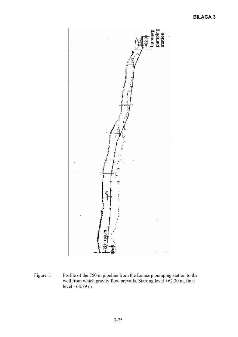
BILAGA 3

3-25

Figure 1. Profile of the 750 m pipeline from the Lunnarp pumping station to the

well from which gravity flow prevails. Starting level +62.30 m, final level +68.79 m

BILAGA 3

3-26

Fig 1a. Sketch of the Lunnarp pumping station with the new pumping station

(new pump) and the old pumping station (old pump) interconnected. There are check valves downstream all pumps

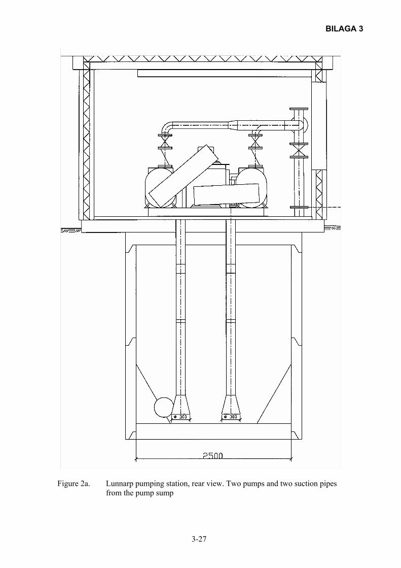
BILAGA 3

3-27

Figure 2a. Lunnarp pumping station, rear view. Two pumps and two suction pipes

from the pump sump

BILAGA 3

3-28

Figure 2b. Lunnarp pumping station, view from the side. Notice the suction pipe

with inlet cone and some bends

BILAGA 3

3-29

Figure 2c. Lunnarp pumping station, view from above

BILAGA 3

3-30

Figure 3. Photo of the pumping station. Upper part of the suction pipes and their

connections to the pumps. The air valve is clearly seen on the right hand pump. The check valve on the pressure side is seen immediately above the air valve. The two pumps are attached to the single pipeline on the pressure side. Also notice the three 900 elbows on the suction pipes immediately upstream the pumps

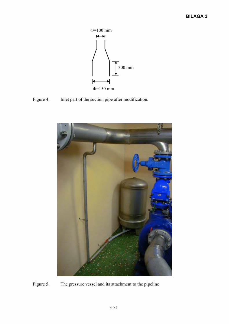
BILAGA 3

3-31

Φ=100 mm 300 mm Φ=150 mm Figure 4. Inlet part of the suction pipe after modification.

Figure 5. The pressure vessel and its attachment to the pipeline

BILAGA 3

3-32

Figure 6. Lunnarp pumping station. Piping on the pressure side with a ball valve at

the highest point for air release of possible entrapped air. This point was also used for pressure measurements downstream of the second check valve

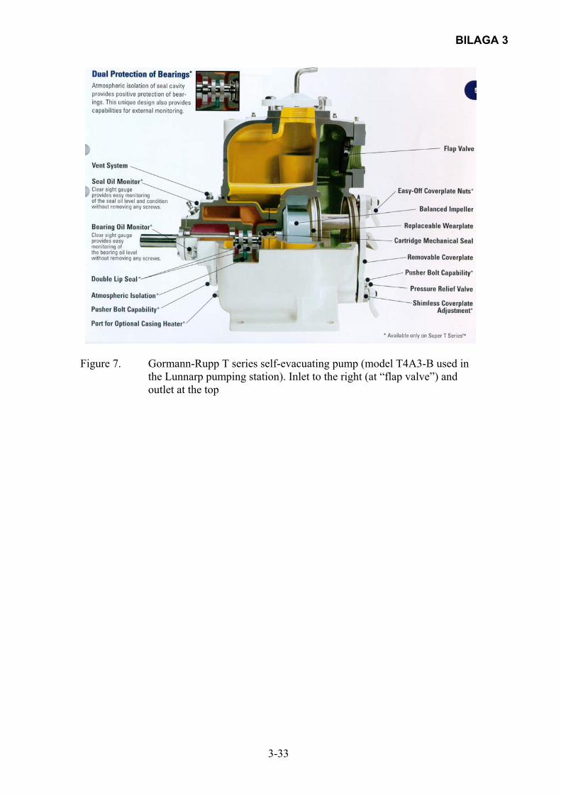
BILAGA 3

3-33

Figure 7. Gormann-Rupp T series self-evacuating pump (model T4A3-B used in

the Lunnarp pumping station). Inlet to the right (at “flap valve”) and outlet at the top

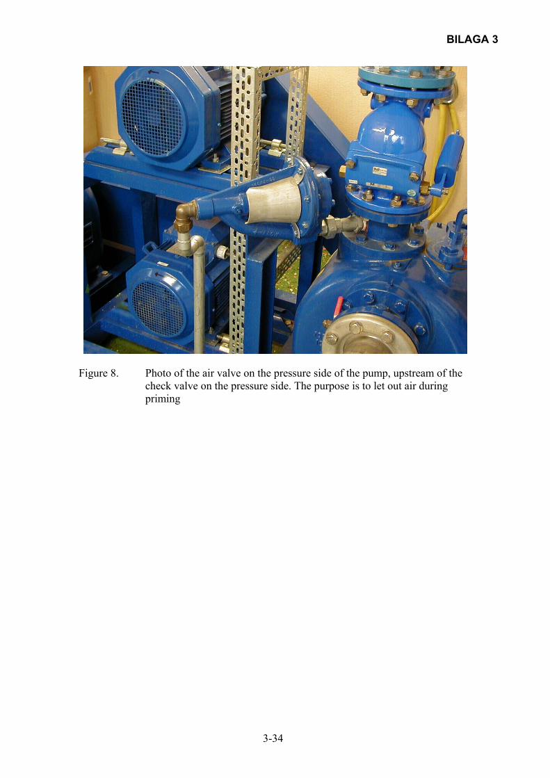
BILAGA 3

3-34

Figure 8. Photo of the air valve on the pressure side of the pump, upstream of the

check valve on the pressure side. The purpose is to let out air during priming

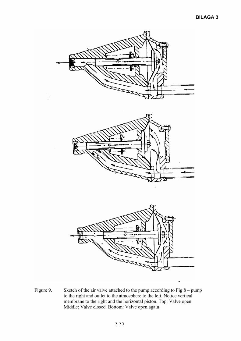
BILAGA 3

3-35

Figure 9. Sketch of the air valve attached to the pump according to Fig 8 – pump

to the right and outlet to the atmosphere to the left. Notice vertical membrane to the right and the horizontal piston. Top: Valve open. Middle: Valve closed. Bottom: Valve open again

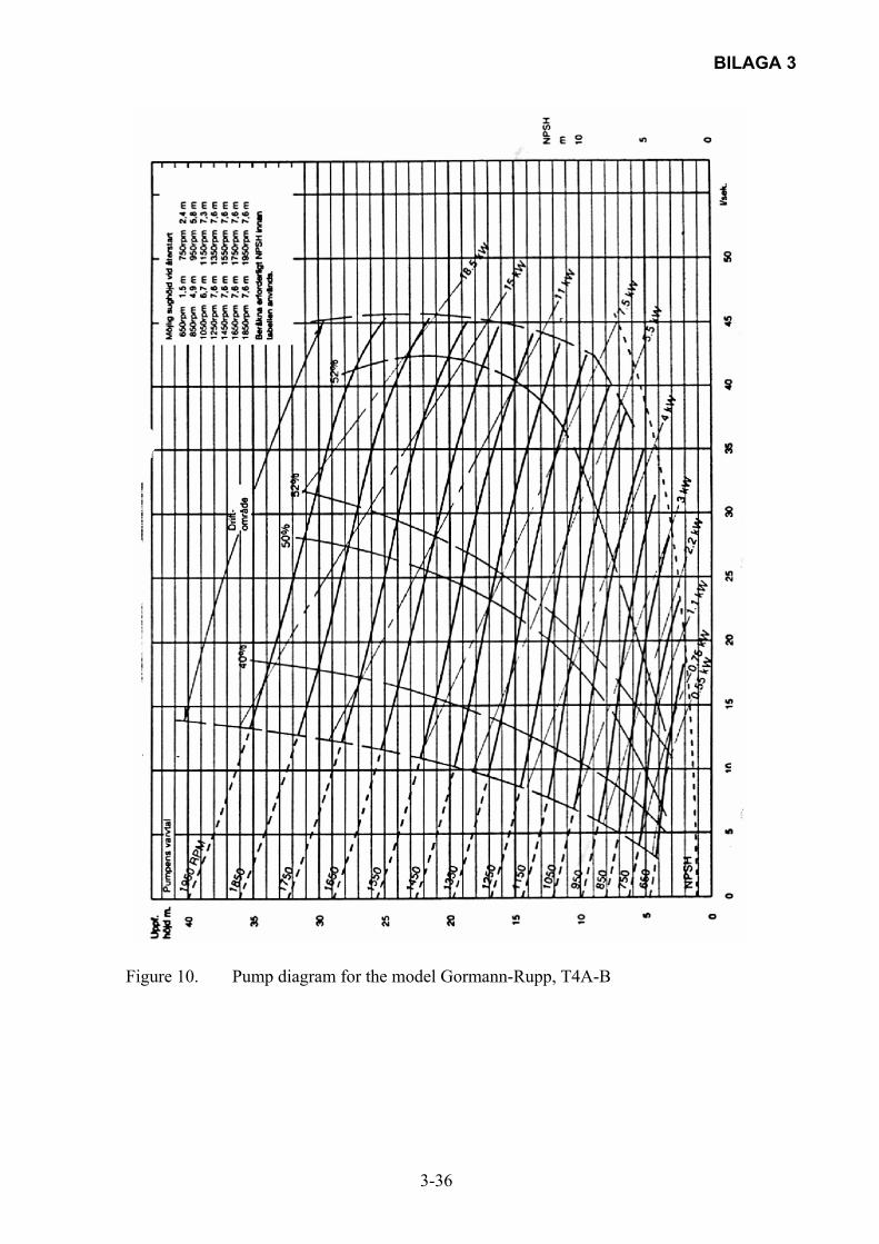
BILAGA 3

3-36

Figure 10. Pump diagram for the model Gormann-Rupp, T4A-B

BILAGA 3

3-37

Figure 11. Calibration curve for the 25 bar pressure transducer

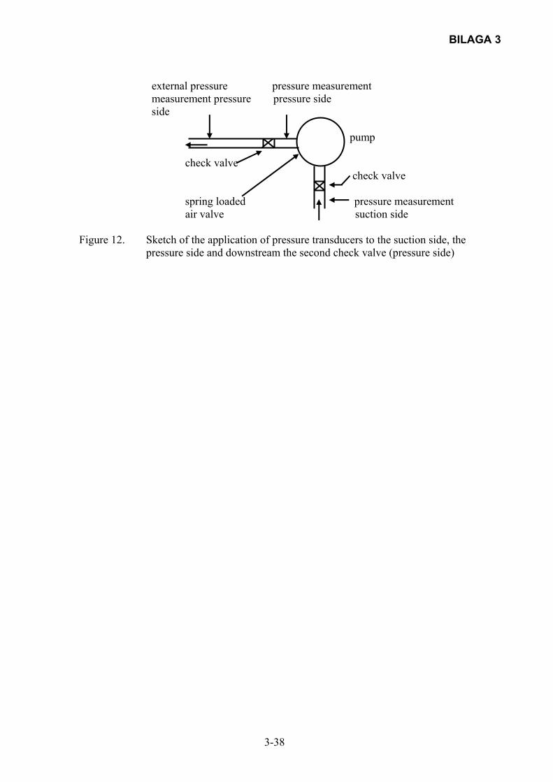
BILAGA 3

3-38

external pressure pressure measurement measurement pressure pressure side side

p pump check valve check valve spring loaded pressure measurement air valve suction side Figure 12. Sketch of the application of pressure transducers to the suction side, the

pressure side and downstream the second check valve (pressure side)

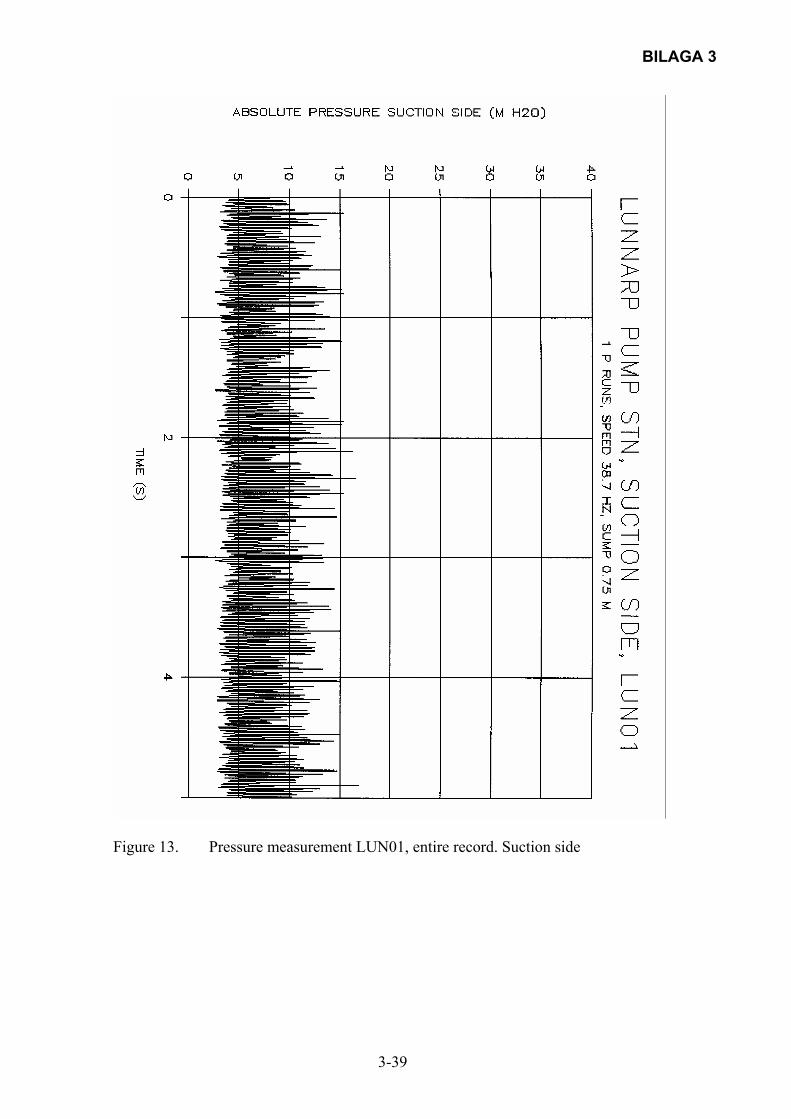
BILAGA 3

3-39

Figure 13. Pressure measurement LUN01, entire record. Suction side

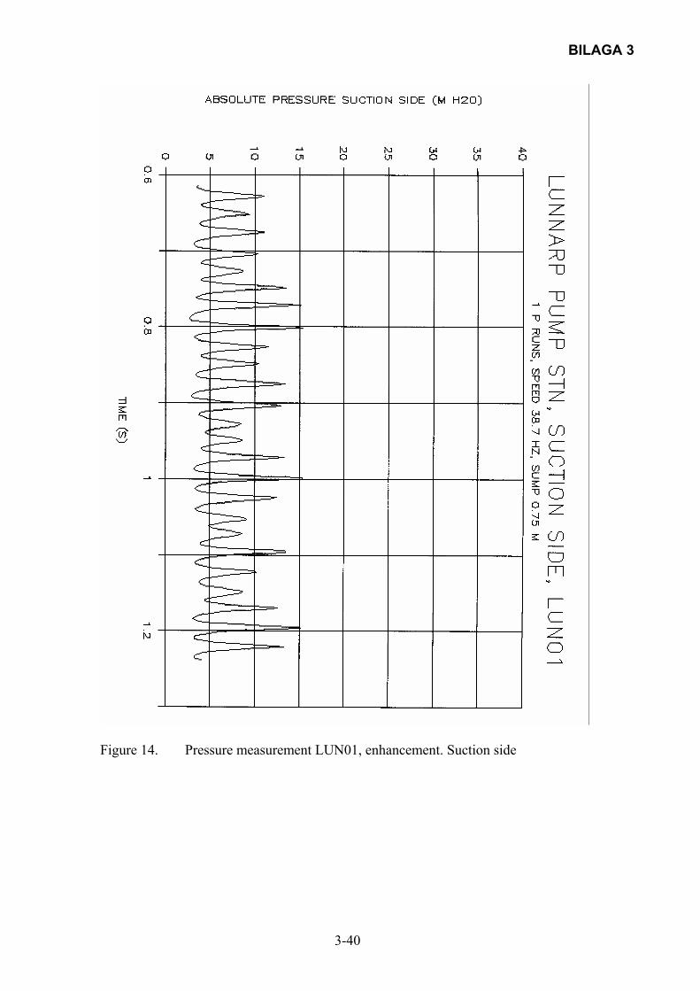
BILAGA 3

3-40

Figure 14. Pressure measurement LUN01, enhancement. Suction side

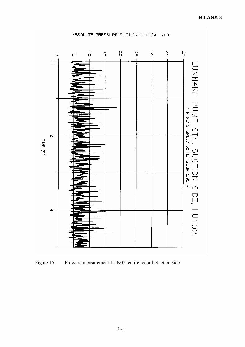
BILAGA 3

3-41

Figure 15. Pressure measurement LUN02, entire record. Suction side

BILAGA 3

3-42

Figure 16. Pressure measurement LUN02, enhancement. Suction side

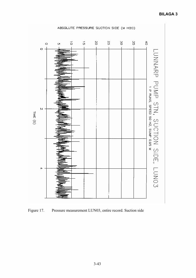
BILAGA 3

3-43

Figure 17. Pressure measurement LUN03, entire record. Suction side

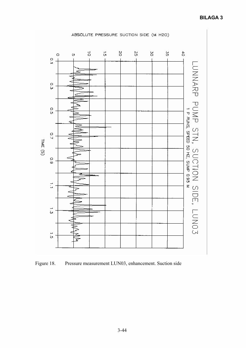
BILAGA 3

3-44

Figure 18. Pressure measurement LUN03, enhancement. Suction side

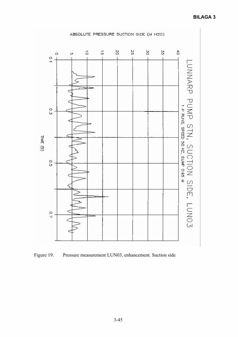
BILAGA 3

3-45

Figure 19. Pressure measurement LUN03, enhancement. Suction side

BILAGA 3

3-46

Figure 20. Pressure measurement LUN04, entire record. Suction side

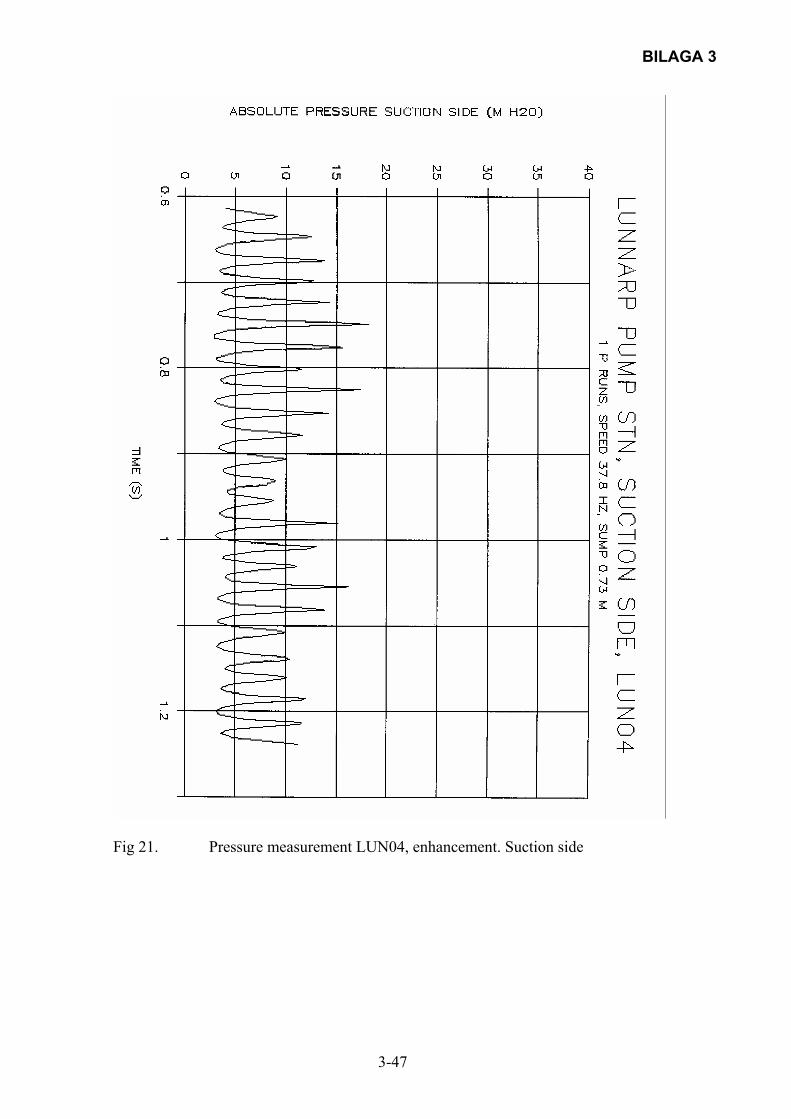
BILAGA 3

3-47

Fig 21. Pressure measurement LUN04, enhancement. Suction side

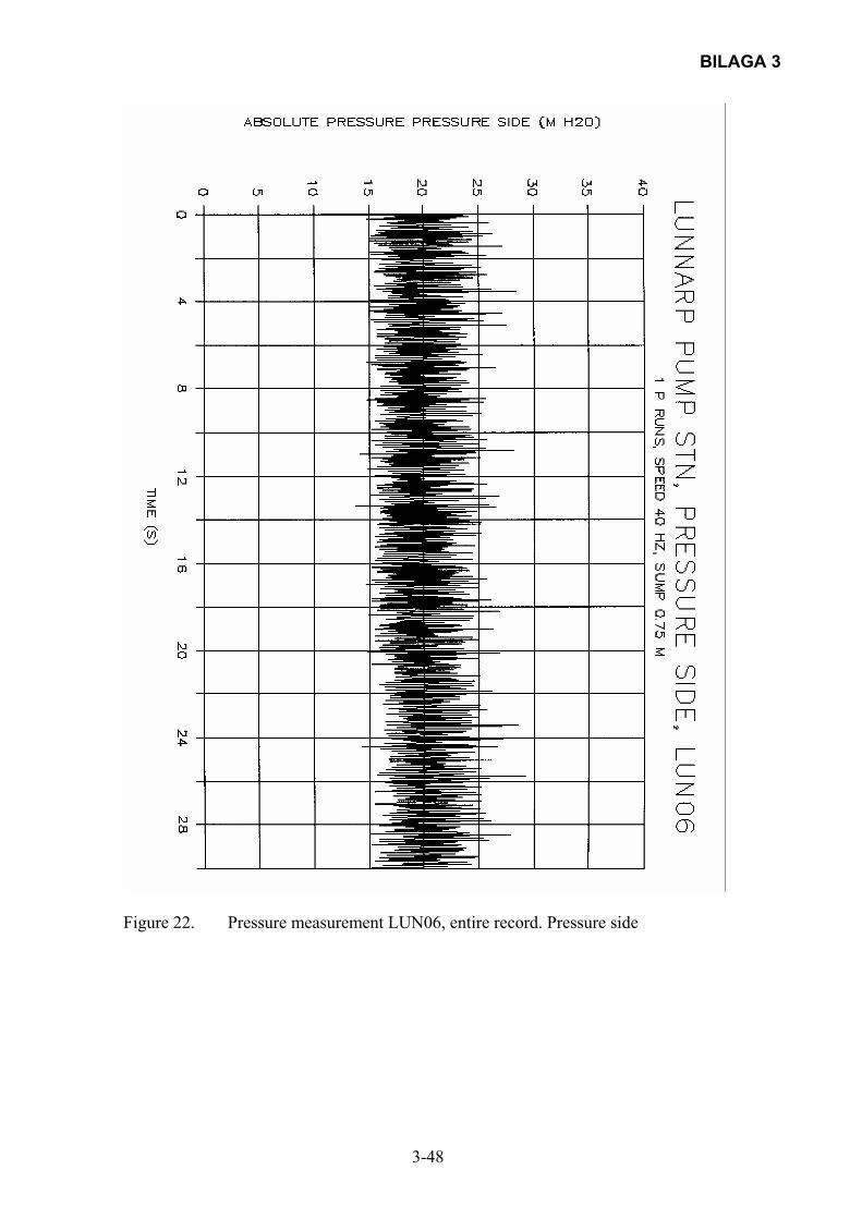
BILAGA 3

3-48

Figure 22. Pressure measurement LUN06, entire record. Pressure side

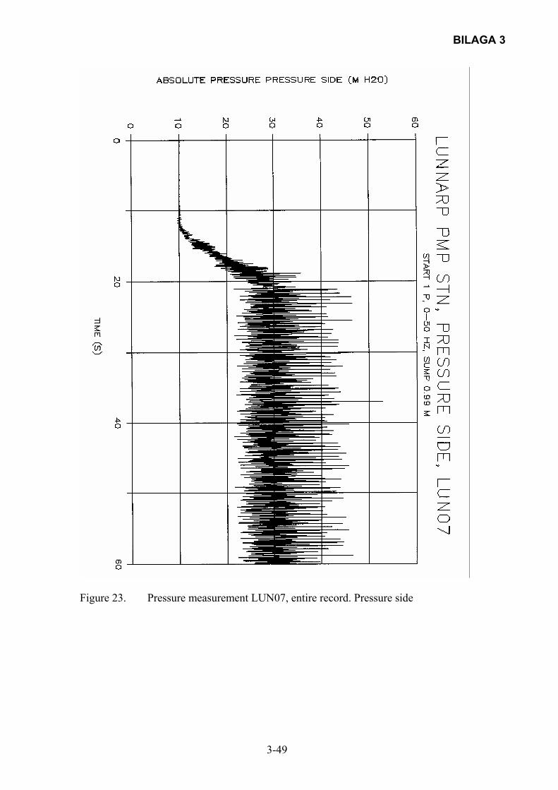
BILAGA 3

3-49

Figure 23. Pressure measurement LUN07, entire record. Pressure side

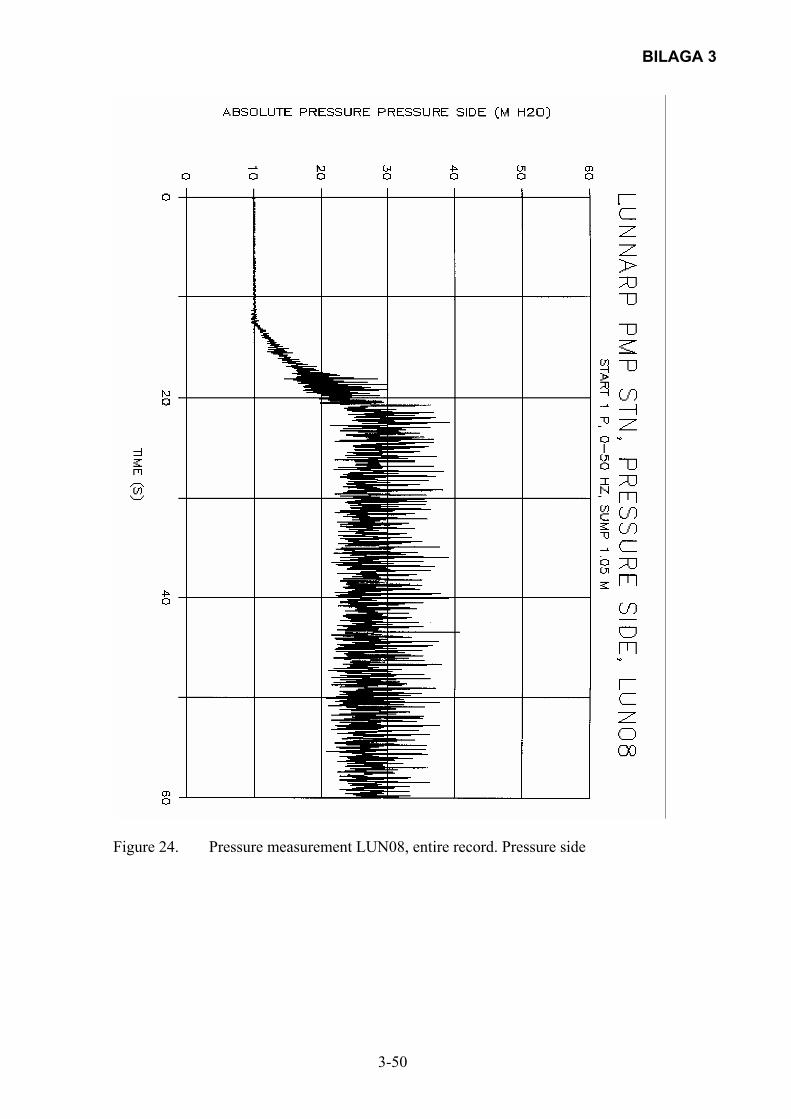
BILAGA 3

3-50

Figure 24. Pressure measurement LUN08, entire record. Pressure side

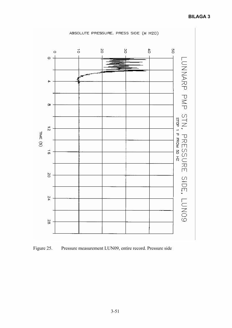
BILAGA 3

3-51

Figure 25. Pressure measurement LUN09, entire record. Pressure side

BILAGA 3

3-52

Fig 26. Pressure measurement LUN10, entire record. Suction side and pressure

side respectively

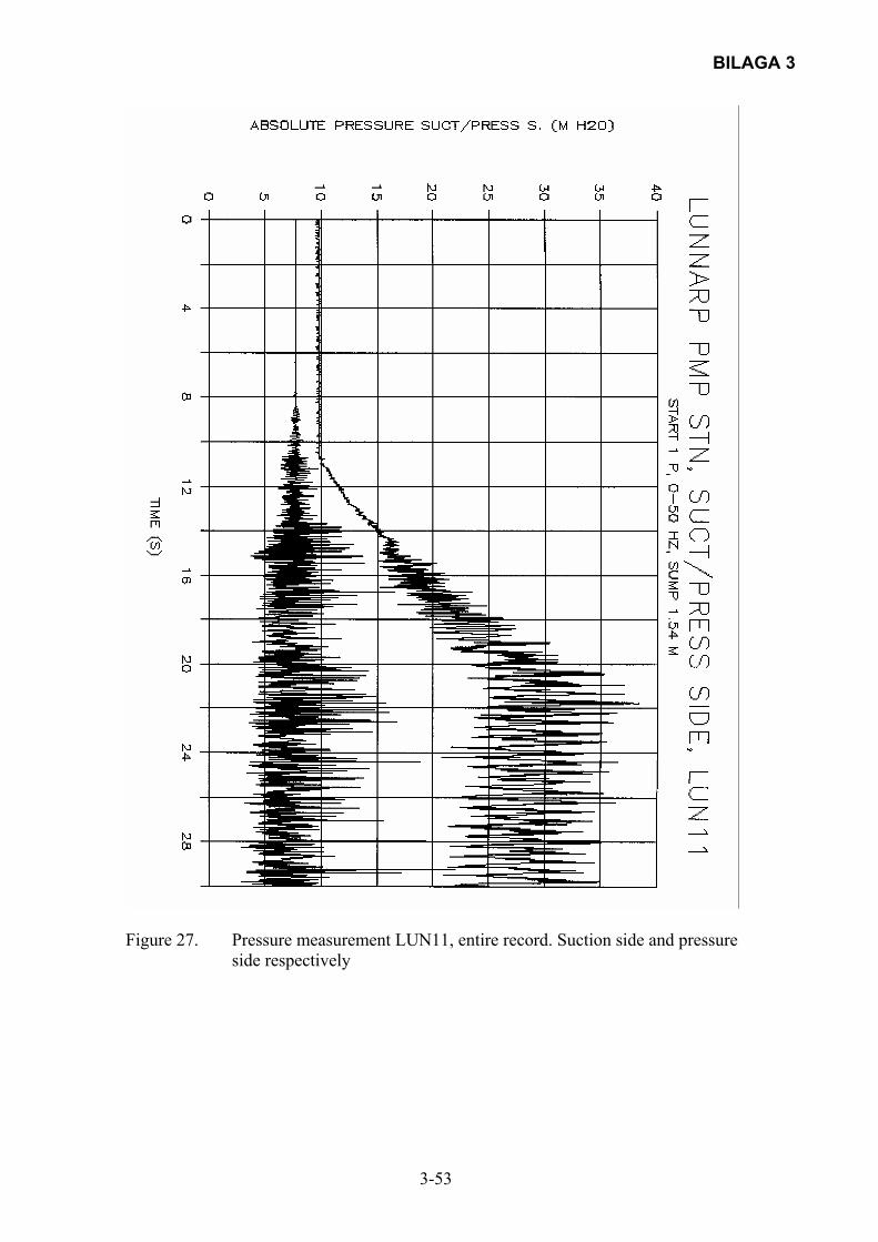
BILAGA 3

3-53

Figure 27. Pressure measurement LUN11, entire record. Suction side and pressure

side respectively

BILAGA 3

3-54

Figure 28. Pressure measurement LUN12, entire record. Suction side and pressure

side respectively

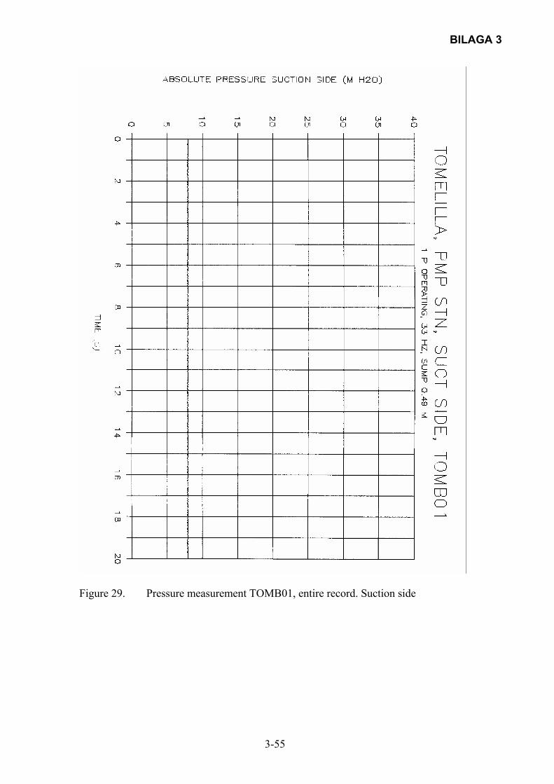
BILAGA 3

3-55

Figure 29. Pressure measurement TOMB01, entire record. Suction side

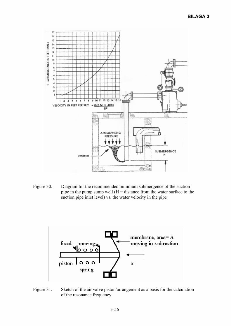
BILAGA 3

3-56

Figure 30. Diagram for the recommended minimum submergence of the suction

pipe in the pump sump well (H = distance from the water surface to the suction pipe inlet level) vs. the water velocity in the pipe

Figure 31. Sketch of the air valve piston/arrangement as a basis for the calculation

of the resonance frequency

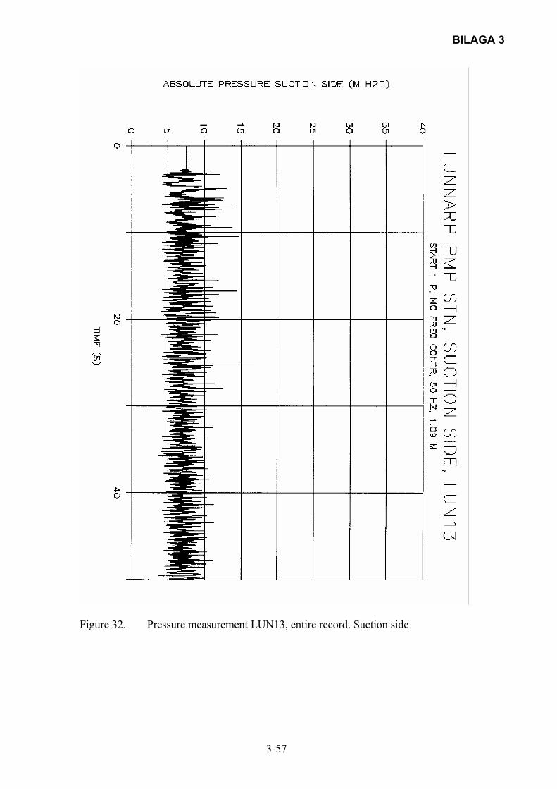
BILAGA 3

3-57

Figure 32. Pressure measurement LUN13, entire record. Suction side

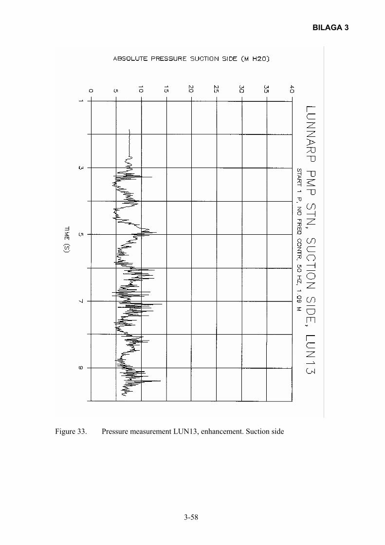
BILAGA 3

3-58

Figure 33. Pressure measurement LUN13, enhancement. Suction side

BILAGA 3

3-59

Figure 34. Pressure measurement LUN13, enhancement. Suction side

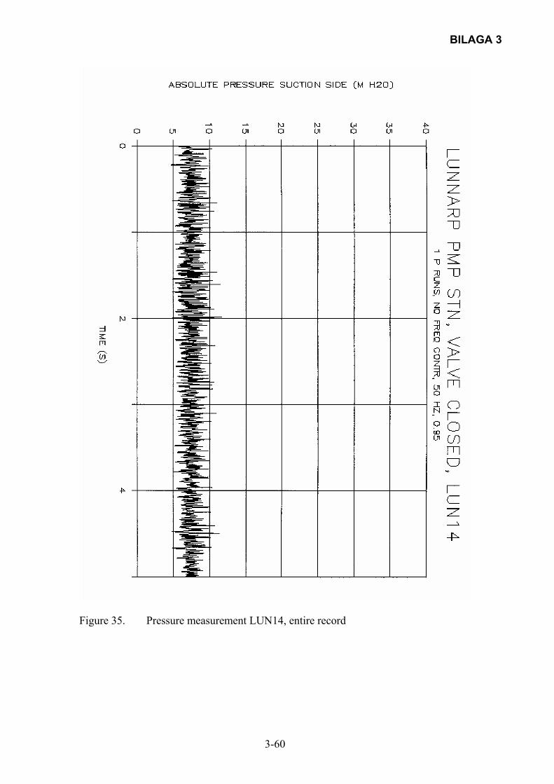
BILAGA 3

3-60

Figure 35. Pressure measurement LUN14, entire record

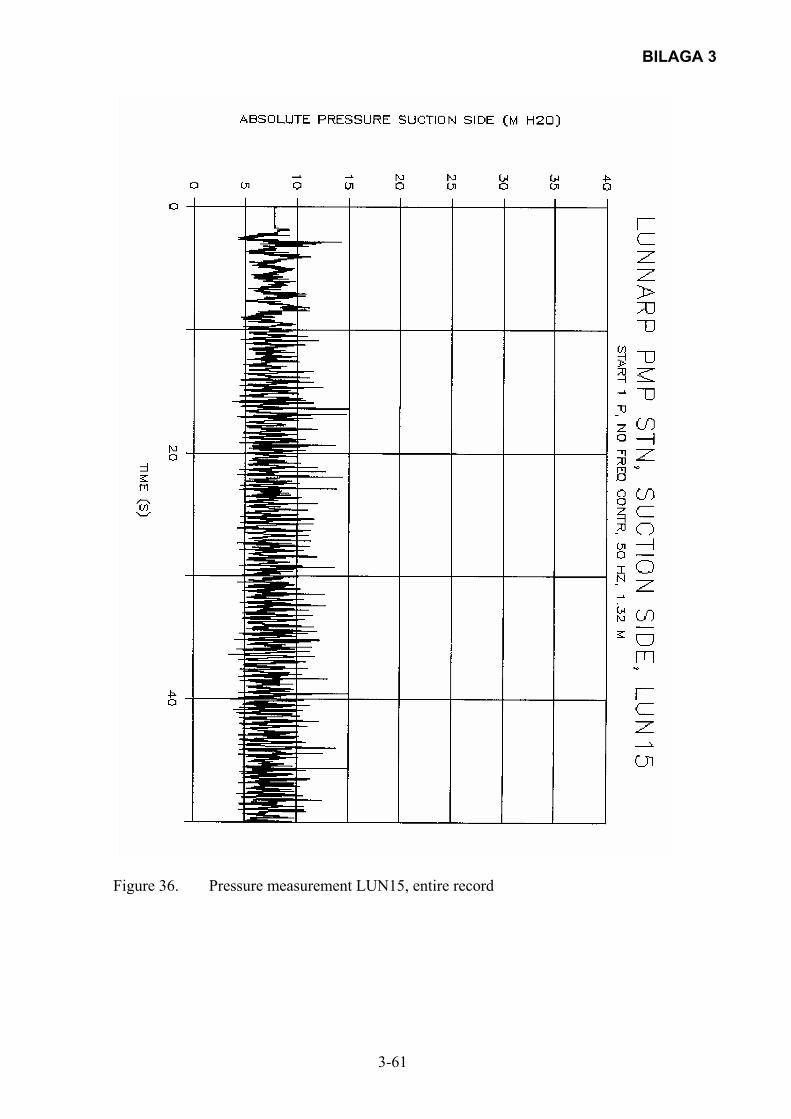
BILAGA 3

3-61

Figure 36. Pressure measurement LUN15, entire record

BILAGA 3

3-62

Figure 37. Pressure measurement LUN15, enhancement

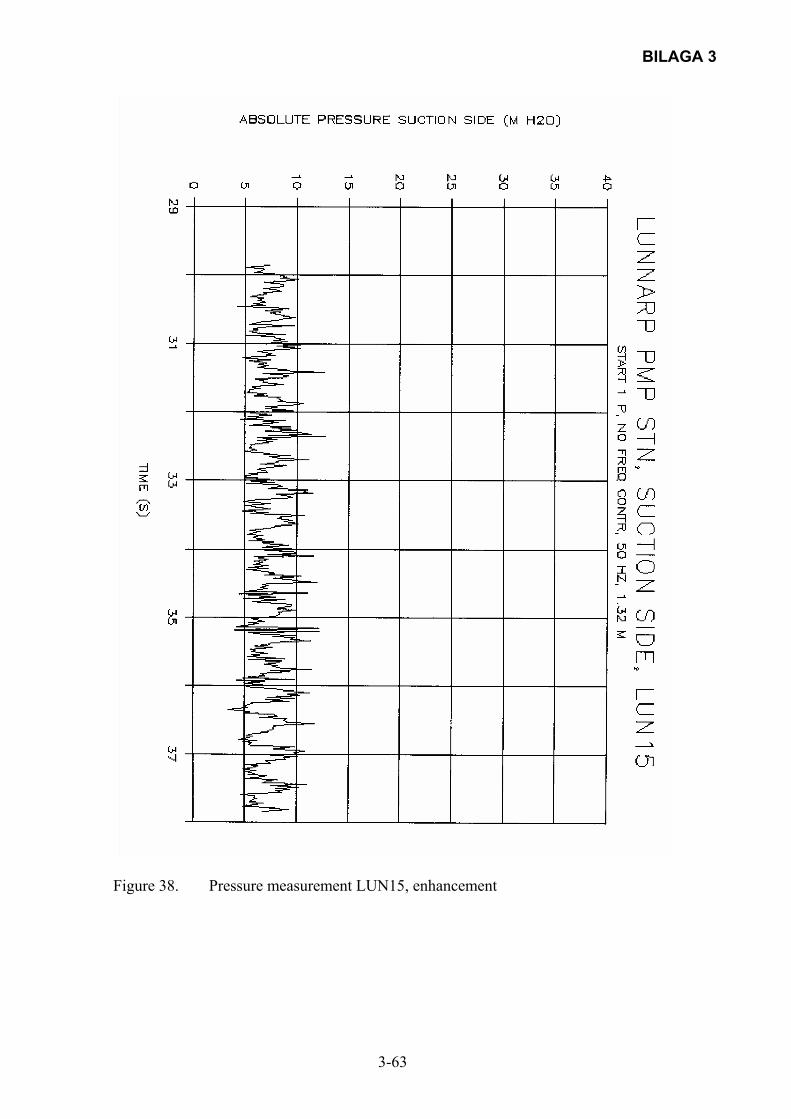
BILAGA 3

3-63

Figure 38. Pressure measurement LUN15, enhancement

BILAGA 3

3-64

Figure 39. Pressure measurement LUN16, entire record. Suction side and pressure

side respectively

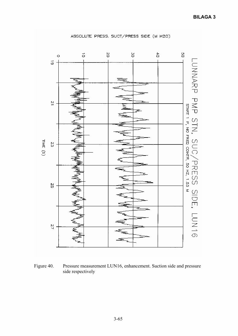
BILAGA 3

3-65

Figure 40. Pressure measurement LUN16, enhancement. Suction side and pressure

side respectively

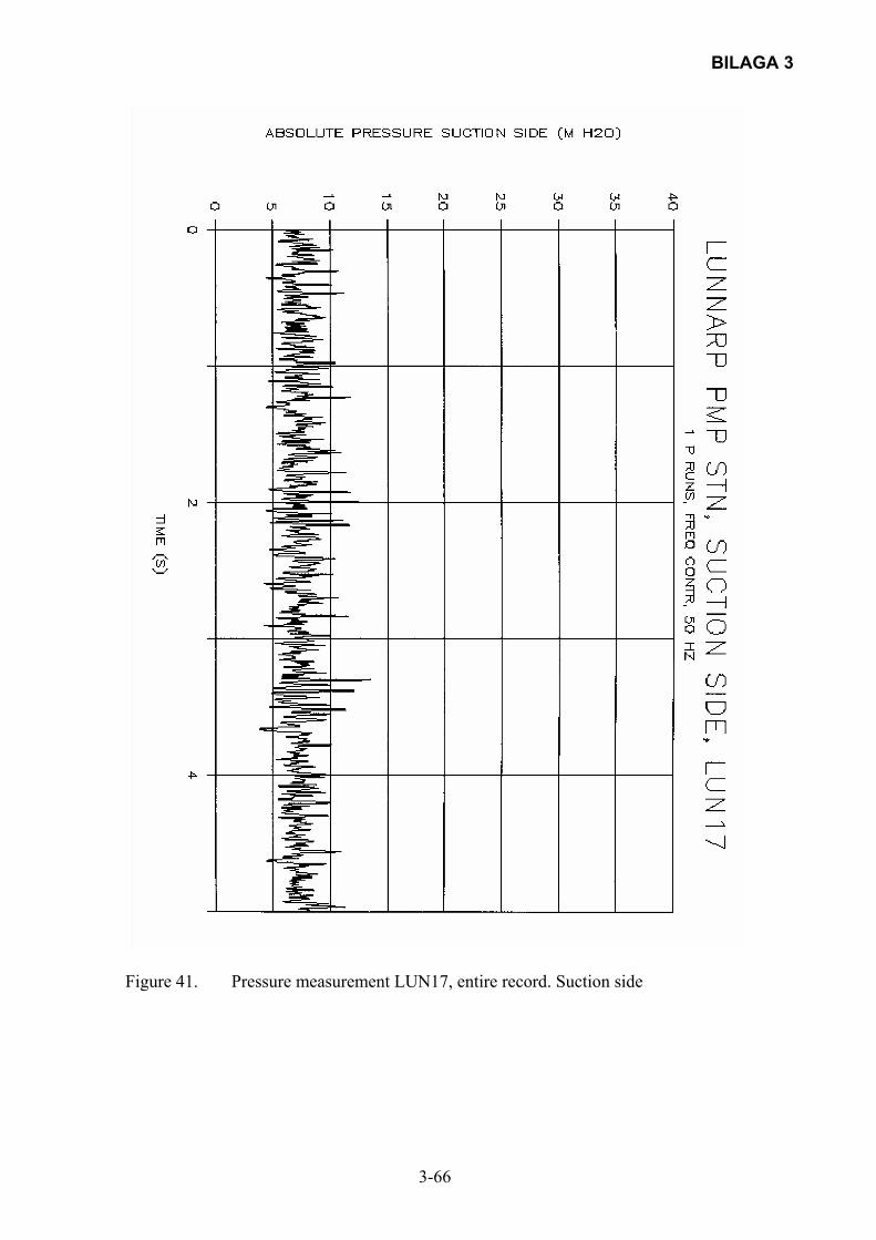
BILAGA 3

3-66

Figure 41. Pressure measurement LUN17, entire record. Suction side

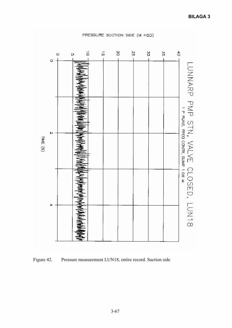
BILAGA 3

3-67

Figure 42. Pressure measurement LUN18, entire record. Suction side

BILAGA 3

3-68

Figure 43. Pressure measurement LUN19, entire record. Suction and pressure sides

respectively

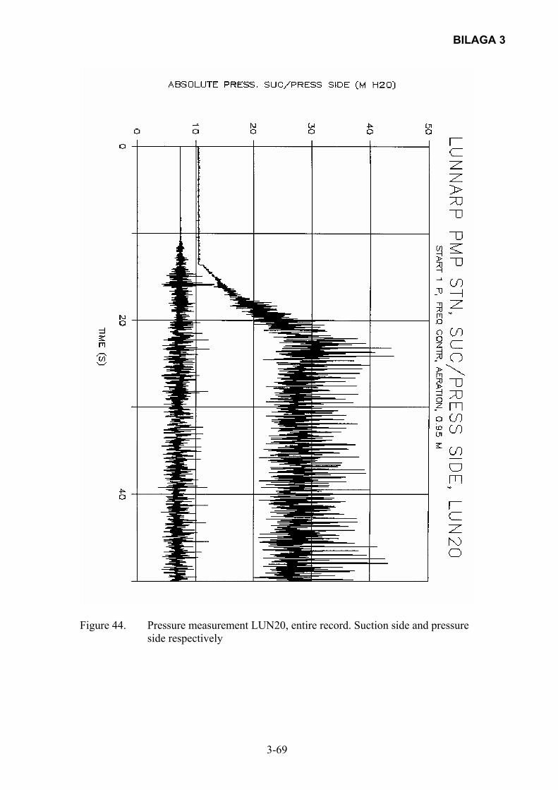
BILAGA 3

3-69

Figure 44. Pressure measurement LUN20, entire record. Suction side and pressure

side respectively

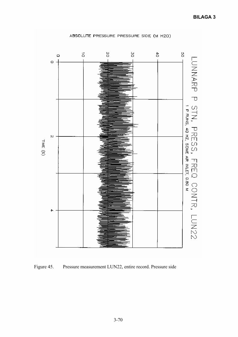
BILAGA 3

3-70

Figure 45. Pressure measurement LUN22, entire record. Pressure side

BILAGA 3

3-71

Figure 46. Pressure measurement LUN22, enhancement. Pressure side

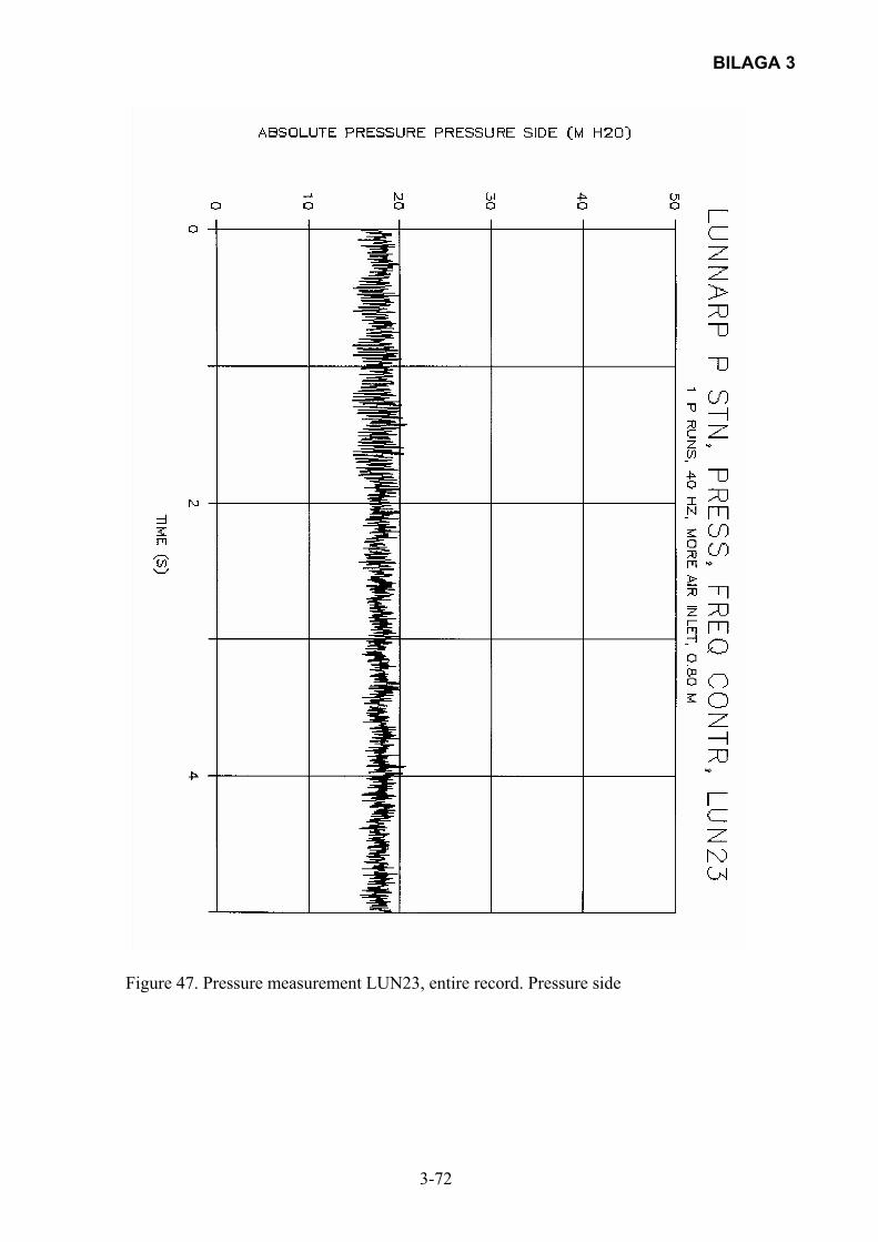
BILAGA 3

3-72

Figure 47. Pressure measurement LUN23, entire record. Pressure side

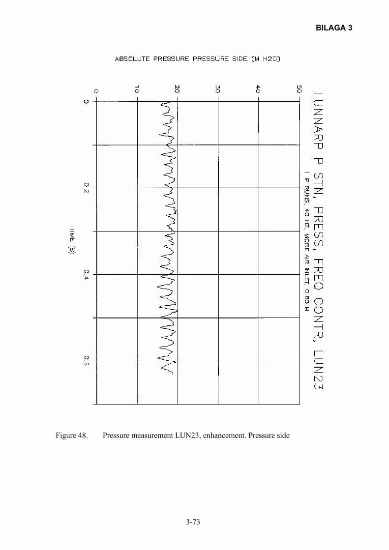
BILAGA 3

3-73

Figure 48. Pressure measurement LUN23, enhancement. Pressure side

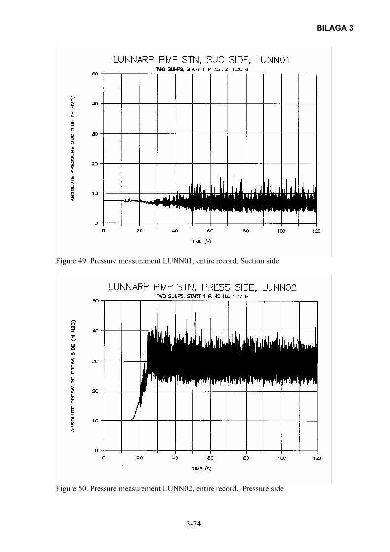
BILAGA 3

3-74

Figure 49. Pressure measurement LUNN01, entire record. Suction side

Figure 50. Pressure measurement LUNN02, entire record. Pressure side

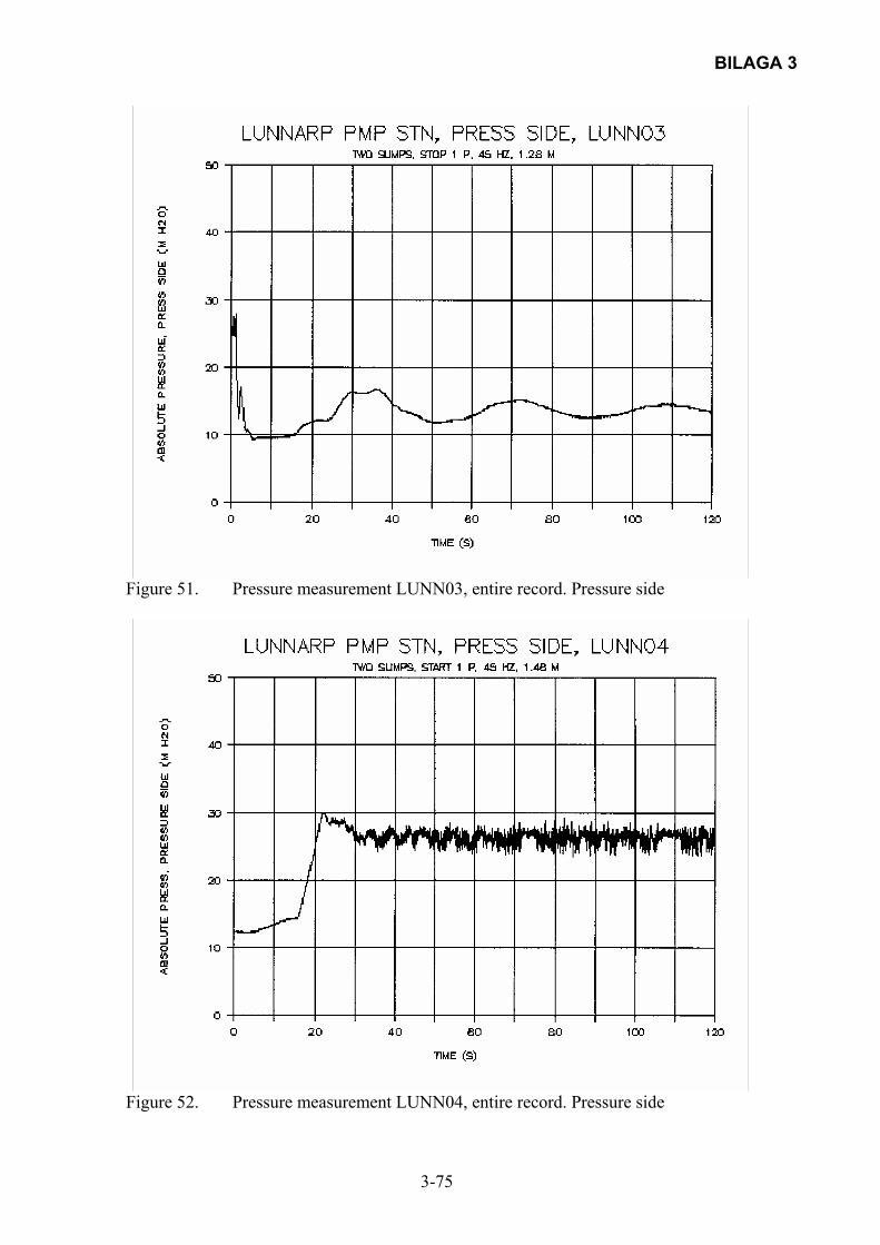
BILAGA 3

3-75

Figure 51. Pressure measurement LUNN03, entire record. Pressure side

Figure 52. Pressure measurement LUNN04, entire record. Pressure side

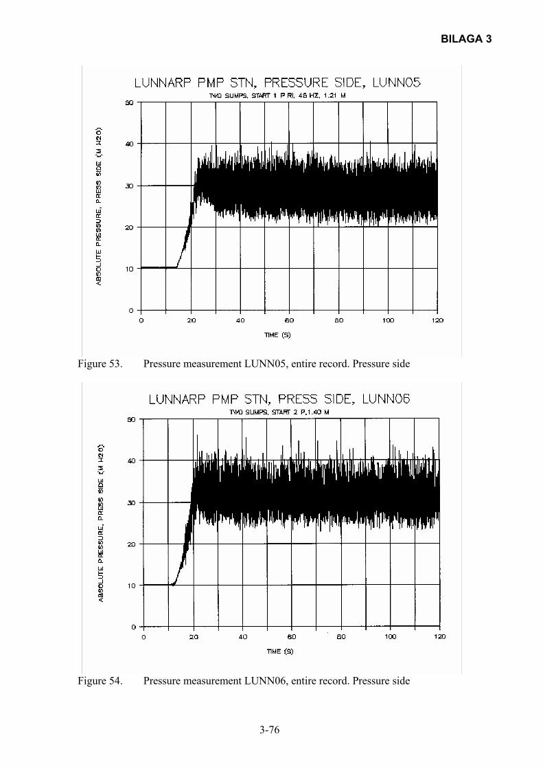
BILAGA 3

3-76

Figure 53. Pressure measurement LUNN05, entire record. Pressure side

Figure 54. Pressure measurement LUNN06, entire record. Pressure side

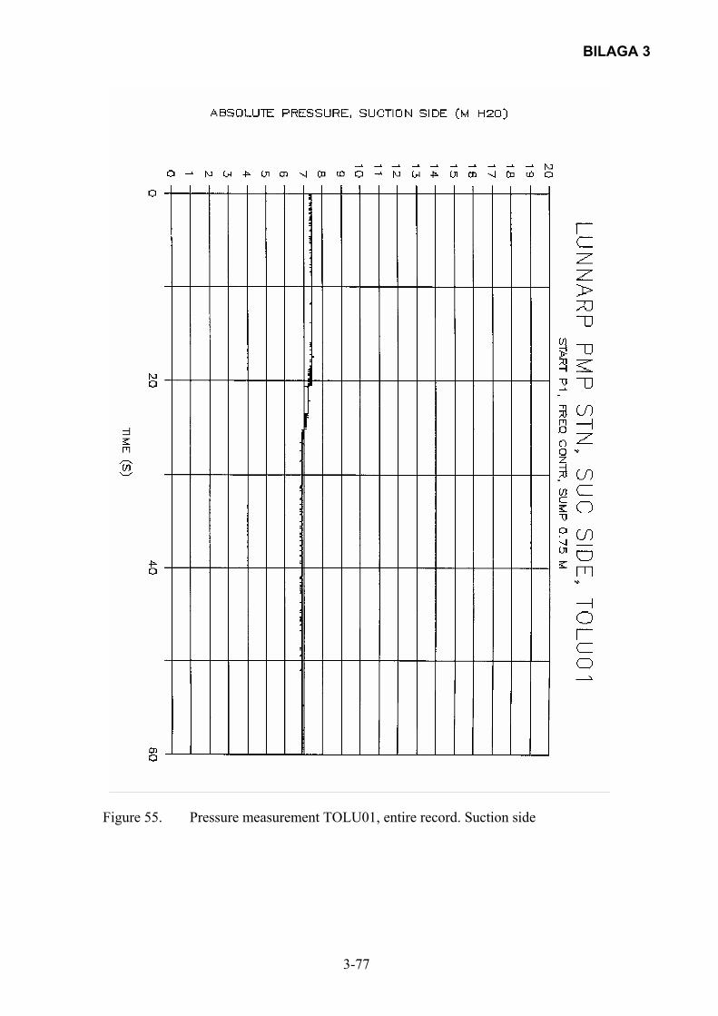
BILAGA 3

3-77

Figure 55. Pressure measurement TOLU01, entire record. Suction side

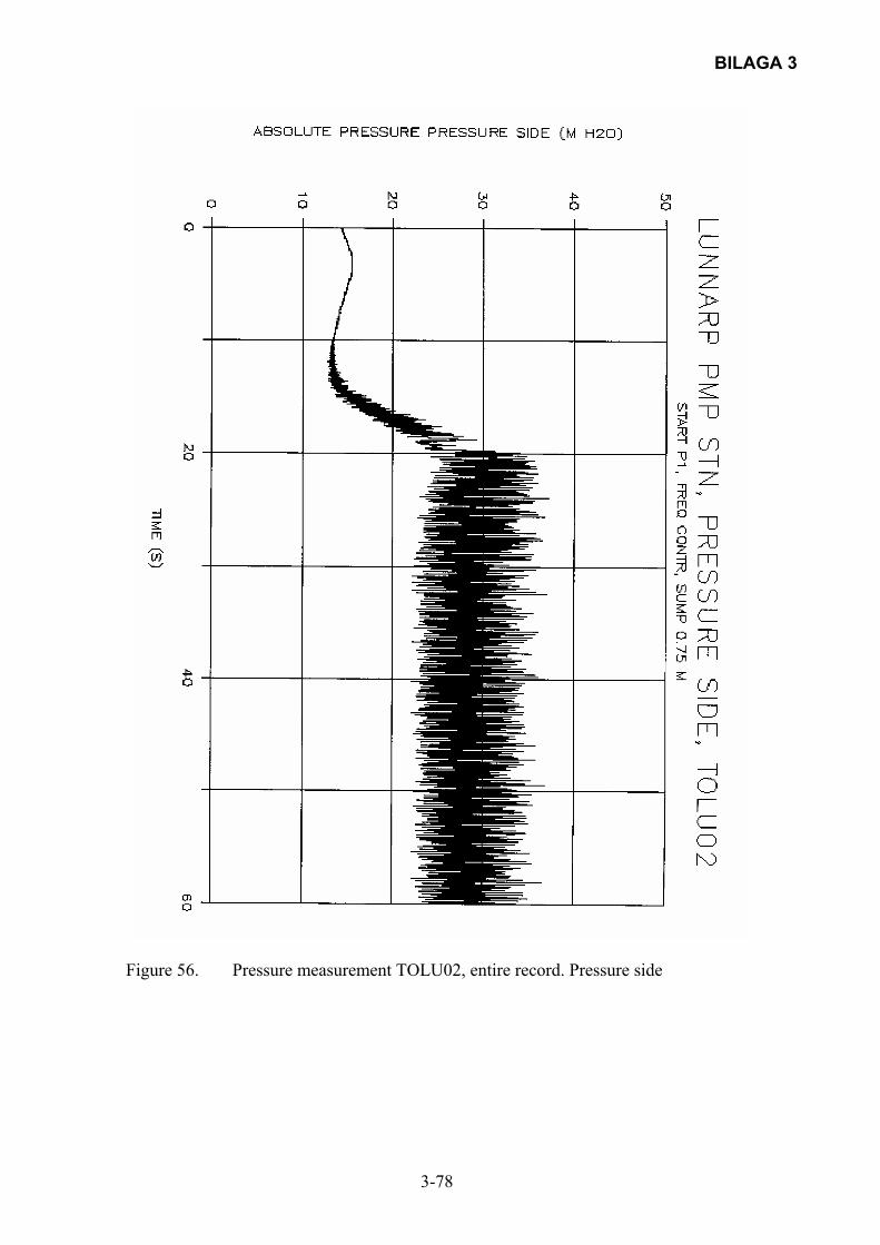
BILAGA 3

3-78

Figure 56. Pressure measurement TOLU02, entire record. Pressure side

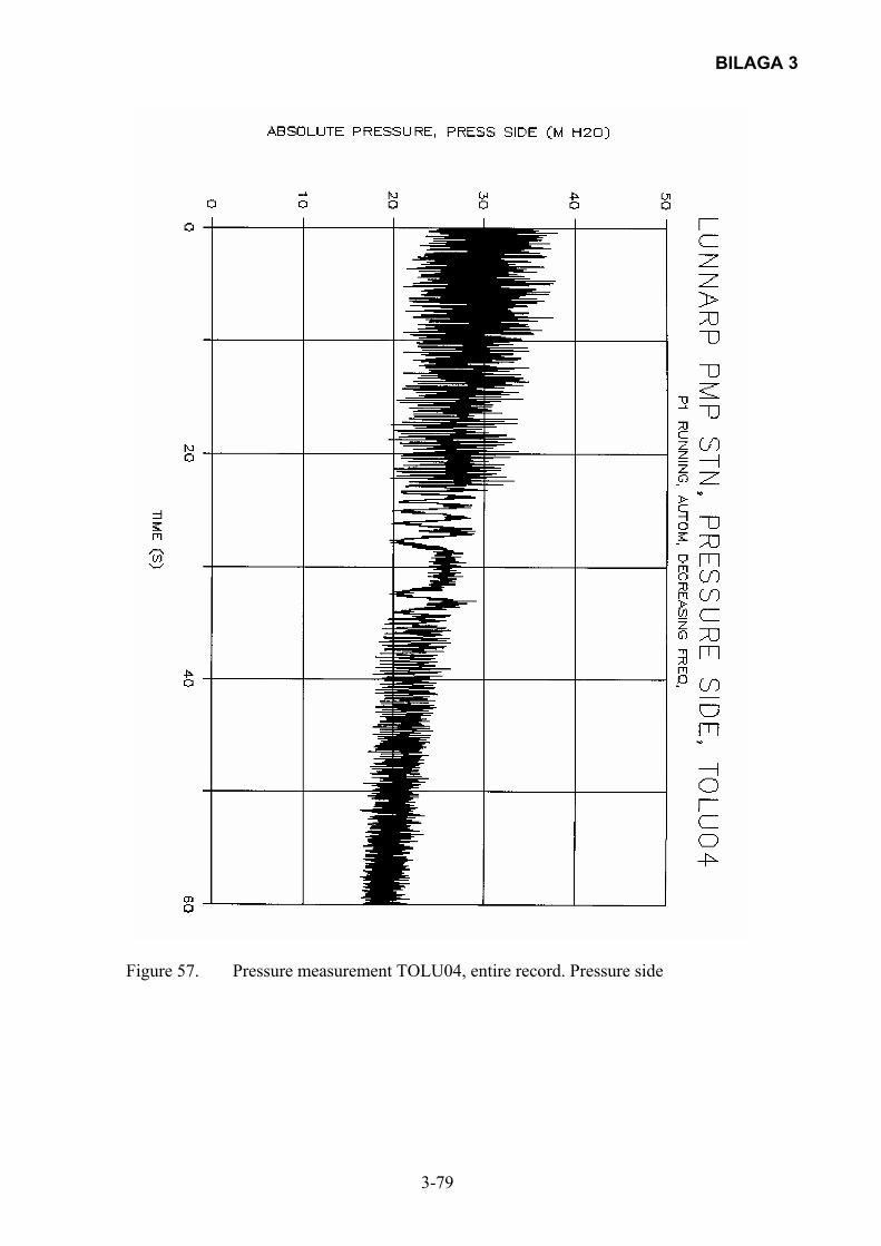
BILAGA 3

3-79

Figure 57. Pressure measurement TOLU04, entire record. Pressure side

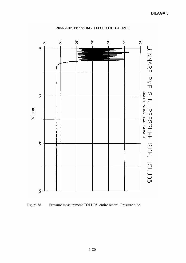
BILAGA 3

3-80

Figure 58. Pressure measurement TOLU05, entire record. Pressure side

BILAGA 3

3-81

Figure 59. Pressure measurement TOLU06, entire record. Pressure side

BILAGA 3

3-82

Figure 60. Pressure measurement TOLU07, entire record. Pressure side

BILAGA 3

3-83

Figure 61. Pressure measurement TOLU08, entire record. Pressure side

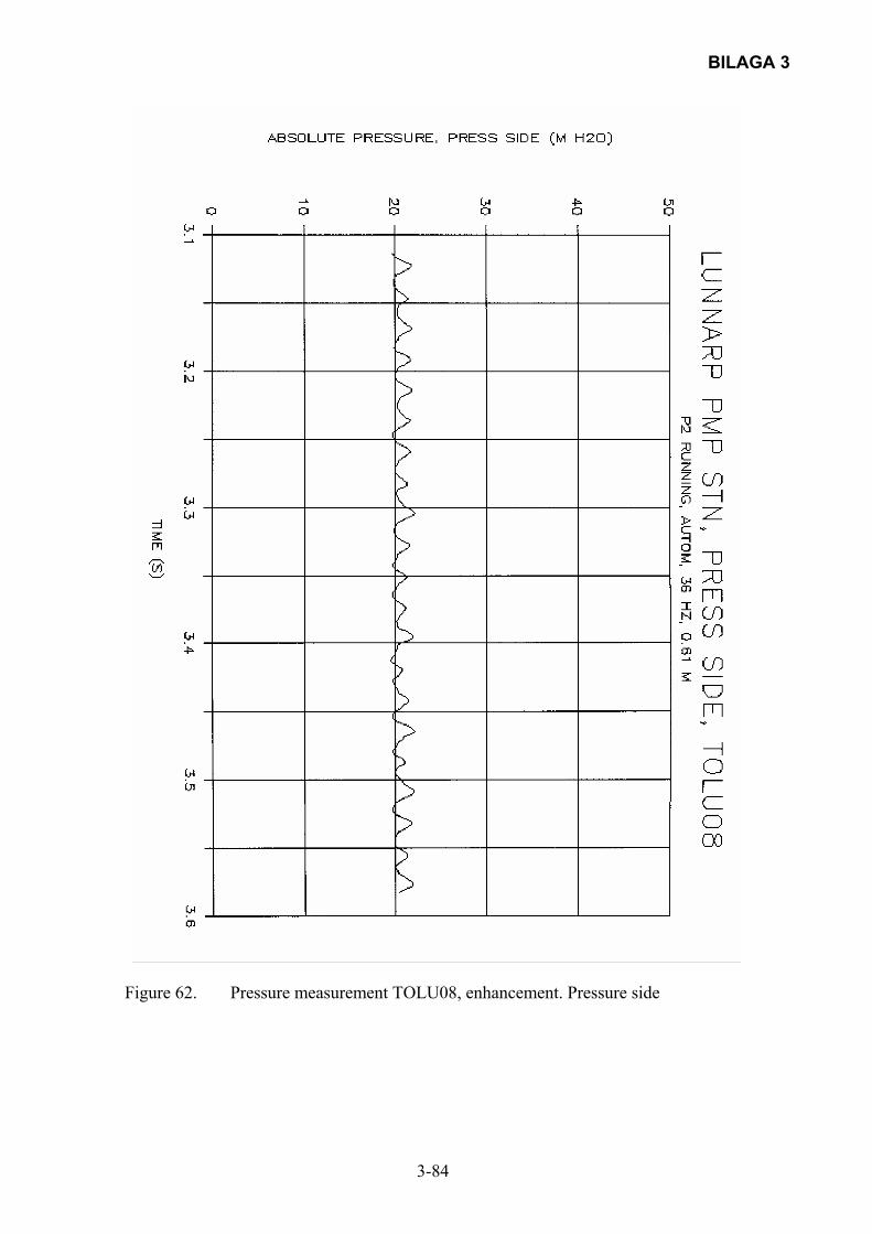
BILAGA 3

3-84

Figure 62. Pressure measurement TOLU08, enhancement. Pressure side

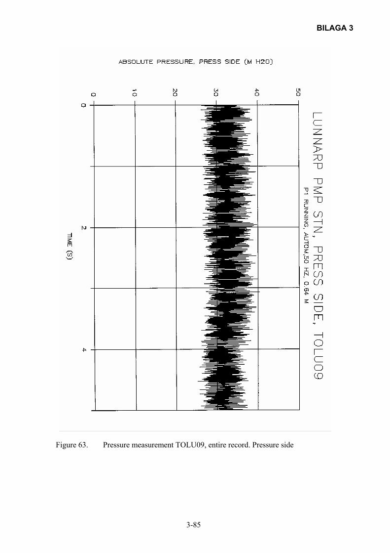
BILAGA 3

3-85

Figure 63. Pressure measurement TOLU09, entire record. Pressure side

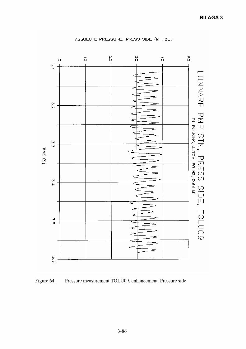
BILAGA 3

3-86

Figure 64. Pressure measurement TOLU09, enhancement. Pressure side

BILAGA 3

3-87

Figure 65. Pressure measurement TOLU10, entire record. Suction side

BILAGA 4

DEPARTMENT OF WATER RESOURCES ENGINEERING LUND INSTITUTE OF TECHNOLOGY, LUND UNIVERSITY

CODEN:LUTVDG/(TVVR-3240)/1-35(2002)

THE EFFECT OF A GAS POCKET IN A PIPELINE ON HYDRAULIC TRANSIENTS – COMPUTER STUDY

by

Lennart Jönsson

The research reported in this document has been made possible through the sponsorship by Ångpanneföreningens Forskningsstiftelse, Stockholm, Sweden and by VA-Forsk,

Stockholm, Sweden

BILAGA 4

CONTENTS page Abstract......................................................................................................... 4-1 Acknowledgement ........................................................................................ 4-1 Introduction .................................................................................................. 4-2 Computational model ................................................................................... 4-2 Inner points ................................................................................................... 4-3 Boundary point, upper reservoir i = 1 .......................................................... 4-3 Boundary point, lower reservoir i = N.......................................................... 4-4 Boundary point. air pocket i = M ................................................................. 4-4 Computations................................................................................................ 4-6 Discussion and conclusion ......................................................................... 4-10 References .................................................................................................. 4-11 Figures 1–19b ............................................................................................. 4-11 Appendix 1, Computer program transgas1.for ........................................... 4-31

BILAGA 4

4-1

ABSTRACT Measurement and careful analysis of hydraulic transients in a water conveying pipeline can provide valuable information on some aspects of the pipeline and its hydraulic properties. One such aspect concerns the existence of limited air/gas pockets in the pipeline, which could affect the capacity and give rise to unsteady flow behaviour. The purpose of this report is to investigate the effect of an air pocket on the characteristics of a hydraulic transient in a single, 1000 m long pipeline. The study is performed by means of a number of computational examples on the basis of the 1-d unsteady, compressible flow equations – the St Venant’s equations – solved using the method of characteristics. The numerical examples are related to a gravity induced flow in a single pipeline, connecting two reservoirs and with a shut-off valve at the downstream end of the pipeline. Transients are generated by closing this valve. Sizes and locations of the air pocket were varied. A comparison with the no-pocket case showed that the air pocket, generally speaking, had a significant effect on the transient. One could distinguish between two major effects, provided the air pocket is not too small:

- a low frequency pressure oscillation is induced by the periodic contraction/expansion of the air pocket

- high frequency pressure oscillation is superimposed on the low frequency oscillation due to pressure waves propagating between the closed valve and the air pocket.

The possibility to obtain the above-mentioned two effects seemed to depend on the location of the air pocket, of course besides the size of the air pocket. Thus:

- for pocket location x = 250 m one could observe the effect down to a pocket length of about 2.5 m

- for pocket location x = 500 m one could observe the effect down to a pocket length of about 0.25 m

- for pocket location x = 750 m one could observe the effect down to a pocket length of about 0.025 m.

The amplitude of the high frequency pressure oscillations, due to wave propagation between the valve and the air pocket, decreased with increasing distance from the valve to the air pocket and with diminishing size of the air pocket. Thus, in the context of using hydraulic transients as a “probing” tool for a single pipeline, indications of the existence of an air/gas pocket should be possible to obtain by analyzing the transient. In the first place the pocket gives rise to a fairly low frequency pressure oscillation, with the typical sharp peaks and more rounded troughs. Secondly, provided sufficient reflection of the pressure waves takes place at the pocket, it should also be possible to locate (at least approximately) the pocket on the basis of the period of the high frequency oscillation and the wave propagation speed. ACKNOWLEDGEMENT This report has been elaborated within the scope of a research project on ”Problems and beneficial use of hydraulic transients” supported by Ångpanneföreningens Forskningsstiftelse and VA-Forsk. This support is gratefully acknowledged.

BILAGA 4

4-2

INTRODUCTION Hydraulic transients occur in pressurized pipelines (i.e. there is no free water surface) for water and wastewater conveyance due to rapid flow changes, normally caused by pump stop/start or valve operation. At the location for the flow change water pressure changes arise which then propagate through the pipeline as pressure waves (see for instance Wylie & Streeter 1975). These pressure waves are most often considered as a problem as they could pose a risk for the operation of the pipeline or, even worse, they could physically damage the pipeline and/or hydraulic components. However, hydraulic transients have also a potential to be considered (and used) in a beneficial and fruitful way. The basic idea is that a hydraulic transient could be regarded as a “probe” propagating back and forth in a pipeline providing some information on the hydraulic status of the pipeline. This is due to the fact that a transient will interact with some properties of a pipeline and affect the characteristics of the transient. Thus, measurement and subsequent, careful analysis of a transient could provide valuable information on several properties of a pipeline and its hydraulic components. In practice, there is most often no need to take any special measures to generate a transient. Pump stop or a valve closure (check valve or a controlled shut-off valve) would be sufficient. It is also, mostly, not a problem to measure the transient by attaching a dynamic pressure transducer to the pipe. A pumping station is a suitable location for several reasons. In the first place it is located close to the transient generating mechanism. Secondly, there is most often an existing tap on the piping that could be used for attaching the transducer. A gas/air pocket of limited extent in a pipeline is such a property which affects the conveying capacity of a pipeline and which also could cause unsteady and unpredictable flow behaviour. A method for determining the possible existence of a gas/air pocket in a pipeline would thus be desirable. A hydraulic transient will most certainly interact with such a pocket as one could expect that part of the pressure wave would be reflected by the pocket due to the very significant elasticity of the gas compared to that of water. The purpose of this report is to investigate computationally the effect of an air pocket on the characteristics of a transient. COMPUTATIONAL MODEL The transient flow and pressure were computed on a simple pipeline, starting at a reservoir and discharging to another reservoir. A shut-off valve was located at the end of the pipeline. The closure of this valve in a prescribed manner generated the transient. The pipeline set-up is illustrated in Fig 1. For the sake of simplicity the pipeline is assumed to start and end at the same level (z = 0). The pipeline input pressure is set to be constant (HIN) at the upstream reservoir and the same goes for the downstream reservoir (HUT). An air pocket with a specified initial volume is assumed to be located at a specified location in the pipeline (vertical coordinate z = zM). The transient computations were based on the ordinary one-dimensional, unsteady, compressible flow equations (St Venant’s equations):

0Ag

axQ

tH 2

=⋅

⋅∂∂

+∂∂ (1)

0DA2

QQf

xHAg

tQ

=⋅⋅

⋅⋅+

∂∂⋅⋅+

∂∂ (2)

BILAGA 4

4-3

where H(x,t) = p/ρg + z = unsteady pressure level Q(x,t) = unsteady flow rate a = pressure wave velocity A = cross sectional area of the pipeline f = frictional coefficient D = pipeline diameter x = axial coordinate t = time The equation of continuity, Eq(1), and the equation of momentum, Eq(2), were solved by means of the method of characteristics (see for instance Jönsson 1975). For that purpose a number of equidistant grid points were defined in the pipeline, i = 1, 2 ,....., N, where i =1 corresponds to the upper reservoir inlet and i = N corresponds to a point immediately upstream of the valve. The air pocket was located at grid point i = M, i.e. without any extent from a grid point of view, Fig 2. The method of characteristics requires that different algorithms are elaborated for inner points; i = 2, 3,....., M-1 and i = M+1, M+2, ...., N-1 and for boundary points; i = 1 (upper reservoir), i = M (air pocket), i = N (valve + downstream reservoir). Moreover, a steady-state solution is required for initiating the computations at t = 0 after which the valve starts closing in a prescribed manner, thus generating the transient phase. Solution of Eqs(1),(2) means that the unknown values of Q, H should be determined in a stepwise manner in time, t = n·∆t (n = 0, 1, 2, ... ) and for every grid point, i = 1, 2,..., N. The distance ∆x between consecutive grid points is determined by the grid point number N, which can be chosen at will. The method of characteristics implies that a specified ∆x will fix the time step ∆t: ∆x= a·∆t (3) INNER POINTS The unknown variables at a later time (n+1)·∆t are denoted Q1(i) and H1(i) respectively. Known variables at the previous time step, n·∆t, are denoted Q(i) and H(i) respectively. According to the method of characteristics, H1(i) and Q1(i) could be determined from:

H1(i) = (HCP(i-1) + HCM(i+1))·0.5 Q1(i) = (H1(i) – HCM(i+1))/B

where HCP(i) = H(i) + B·Q(i) - f·∆x·Q(i)·ABS(Q(i))/(2·g·D·A2) HCM(i) = H(i) - B·Q(i) + f·∆x·Q(i)·ABS(Q(i))/(2·g·D·A2) (4) with B = a/(A·g) ∆x= distance between two consecutive grid points BOUNDARY POINT, UPPER RESERVOIR I = 1 The boundary condition at the upper reservoir is given by: H1(1) = HIN Q1(1) = (H1(1) – HCM(2))/B (5) for t ≥ 0.

BILAGA 4

4-4

BOUNDARY POINT, LOWER RESERVOIR I = N This boundary point is characterized by the valve, immediately followed by the lower reservoir. The valve acts as a head loss:

2ventvent Qkh ⋅=

Thus, the boundary condition is given by: H1(N) = HUT ± kvent· Q1(N)· ABS(Q1(N)) H1(N) = HCP(N-1) - B· Q1(N) (6) where ± in Eq(6) refers to flow into (+) the reservoir and (-) flow out of the reservoir. The valve operation (valve loss) is described on the basis of a prescribed decrease of the pipeline cross section, Fig 3. It is assumed that:

2

öpp

0vent A

A10XKONSTh

−⋅= (7)

where XKONST0 = suitably chosen constant A0 = full pipe cross sectional area Aöpp = (D – x)/D · A0 = cross sectional area during the closure operation (simplified description) x = vertical location of the lower edge of a hypothetical disk moving downwards (0 ≤ x ≤ D). The valve closure starts at t = T0 and continues in a linear fashion until t = T1 after which another, slower closure operation takes place until the valve is fully closed at t = T2, Fig 3. BOUNDARY POINT, AIR POCKET I = M The air pocket is idealized as a “cylinder” with variable length and extending over the entire cross section, Fig 4. Computationally, the air pocket is located at grid point i = M all the time (i.e. no axial extent during the overall transient computations). As the air pocket divides the water column into two separate columns one has to introduce the grid points M1 and M2, coinciding with i = M but with M1 belonging to the left column and M2 belonging to the right hand column respectively. The following equations were used for the transient description of the air pocket: κκ ⋅=⋅ VolpVolp 0 (8) where p = absolute pressure in the air pocket at time t Vol = volume of the air pocket at time t κ = 1.0–1.4 depending on the thermal properties of the air volume changes p0, Vol0 = corresponding values at steady state flow. Eq(8) describes the isothermal/adiabatic behaviour of the air pocket.

BILAGA 4

4-5

dt

dVol)2M(Q)1M(Q n−=− (9)

dt

dVol)2M(1Q)1M(1Q 1n+−=− (10)

Eqs(9),(10) are the equations of continuity at times n·∆t and (n+1)·∆t respectively. H1(M1) = HCP(M-1) - B·Q1(M1) (11) H1(M2) = HCM(M+1) + B·Q1(M2) (12) which are two equations for the C+ and C- characteristics respectively. It is assumed that H1(M1) = H1(M2) all the time. Moreover, Eq(8) is used at time n·∆t as well as at time (n+1)·∆t. Eqs(8),(9),(10),(11),(12) give Q1(M1), Q1(M2), H1(M1), p and Vol. The steady state solution, assuming no air pocket, is easily computed using reservoir levels and pipeline data. The computer program is listed in Appendix 1. Input data for the program are defined in the input data file: gasin.dat and computed pressures etc are obtained in the output data file: gasut.dat. Input data file: XL, DIA, FRIK, VAGH

N, M, HIN, HUT, HATM, ZM XVOL0, XKAPPA, RHO TIDVENT, TIDTOT, EPS T0, T1, T2, XVENT1, XKONST0 IOUTPUT, IHOUTI where XL = length of the pipeline (m) DIA = diameter of the pipeline (m) FRIK = frictional coefficient VAGH = pressure wave propagation velocity (m/s) N = number of grid points in the pipeline (i = 1,2,..,N) M = grid point, i = M, for the air pocket HIN = upper reservoir level (m H2O) HUT = lower reservoir level (m H2O) HATM= absolute atmospheric pressure (10.2 m H2O) ZM = vertical coordinate for the location of the air pocket. Assume z = 0 at pipe inlet and pipe outlet XVOL0 = steady state air pocket volume (m3) XKAPPA = exponent in Eq(8). Set to κ = 1.0 in the program RHO = density of the liquid (water) (kg/m3) TIDVENT = time for complete valve closure (s) TIDTOT = total computation time (s) EPS = numerical value, related to the accuracy of an iteration procedure in the

BILAGA 4

4-6

computation of the pressure level in the air pocket T0 = time for start of valve closure operation (s) T1 = time for change of the rate of valve closure (s) XVENT1 = location of the lower edge of the hypothetical disk in the valve at time T1 (0 ≤ XVENT1 ≤ DIA) (m) XKONST0 = numerical value describing the valve loss coefficient, Eq(7) IOUTPUT = integer describing the type of data in the output file (IOUTPUT = 0,1,2 or 3) IHOUTI = computed pressure in a selected point (i = IHOUTI) in the output file. Table 1 gives an example of a typical input data list: Table 1: Example of input data list (file: gasin.dat)

1000 0.1 0.02 1000 XL DIA FRIK VAGH 101 51 40 30 10.2 30 N M HIN HUT HATM ZM 0.2 1.0 1000 XVOL0 XKAPPA RHO 20 80 0.00001 TIDVENT TIDTOT EPS 1 5 20 0.02 10000 T0 T1 T2 XVENT1 XKONST0 0 30 IOUTPUT IHOUT1

Most of these input data have been kept the same throughout all the computations. Basically, only XVOL0 and M have been varied. This means that the steady state flow has amounted to Qsteady = 0.00775 m3/s, corresponding to a steady state water velocity Vsteady = 0.99 m/s. COMPUTATIONS A number of computations have been performed, varying the size and the location of the air pocket. As can be seen from Table 1, the wave velocity was assumed to be VAGH = a = 1000 m/s. Moreover, the valve started closing after 1 s and was completely closed after 20 s, i.e. a closure time significantly larger than the propagation time µ for a wave from the valve to the pocket and back to the valve (µ = 1 s if the air pocket is located at x = 500 m). However, the effective closure time, i.e. the time during which the valve loss becomes significant, was considerably shorter causing the pressure wave to be rather steep. A reference case was first computed with no air pocket at all in the pipeline. This result is shown in Fig 4a and the input file was the same as for the air pocket cases except for the non-existence of the air pocket. Figs 5a to 11a show the results of the computed transient pressure H(N) at the valve for different sizes of the air pocket located in the middle of the pipeline, M =51. Moreover, diagrams of the pressure in the air pocket, the air pocket size, the pressure at a location upstream of the air pocket are also shown for some of the XVOL0 cases. Table 2 shows the input data file, which thus was kept the same except for the XVOL0 value. Table 2: Input data file for Figs 5 to 11

1000 0.1 0.02 1000 XL DIA FRIK VAGH 101 51 40 30 10.2 30 N M HIN HUT HATM ZM 0.2 1.0 1000 XVOL0 XKAPPA RHO

BILAGA 4

4-7

20 80 0.00001 TIDVENT TIDTOT EPS 1 5 20 0.02 10000 T0 T1 T2 XVENT1 XKONST0 0 30 IOUTPUT IHOUT1

Comments. Figure number to the left refers to all diagrams for a certain XVOL0 value: Fig 5: XVOL0 = 0.5 m3. This is a very large air pocket, corresponding to a pocket length of

64 m. The oscillating pressure has got a time period of T = 2 s, i.e. 4·L1/a = T implying L1 = 500 m for the location of the reflecting point (air pocket). This means that the pocket acts more or less as an artificial reservoir against which pressure waves are reflected.

Fig 6. XVOL0 = 0.2 m3. Very large air pocket, corresponding length 25 m. The oscillating

pressure has got a time period T = 2 s, i.e. implying more or less total reflection at the air pocket. There is also a basic, slow pressure change in the computed pressure due to the expansion/contraction of the air pocket. This is evident from Fig 6b showing the pressure inside the air pocket. Fig 6c shows the corresponding air pocket size, starting with 0.2 m3 and approaching 0.15 m3 asymptotically when all movements have ceased. This is in agreement with the initial steady state pressure in the air pocket: p0/ρg = HM0 - ZM + HATM = 35 - 30 + 10 = 15 m H2O and the final, asymptotic value: p/ρg = HM - ZM + HATM = 40 - 30 + 10 = 20 m H2O. Fig 6d shows the computed pressure upstream of the air pocket (the location is 300 m from the pipeline inlet). It is evident that there is hardly any pressure fluctuation. Thus, the air pocket will not let through the pressure waves, implying the more or less total reflection at the pocket as mentioned above.

Fig 7. XVOL0 = 0.05 m3 corresponding to a pocket length of 6.2 m. The rapid oscillatory

pressure has still got a period of T = 2 s, i.e. corresponding to a very significant reflection. There is also a slow oscillation, although faster than in the case in Fig 6a, due to the air pocket oscillation

Fig 8. XVOL0 = 0.02 m3 corresponding to a pocket length of 2.5 m. The rapid oscillatory

pressure, T = 2 s, implying reflection at the pocket is easily distinguishable. The slower oscillation of the air pocket is also distinct which is also shown in Fig 8b (air pocket pressure). The air pocket size is shown in Fig 8c, with a maximum of about 0.035 m3 and a minimum of about 0.0075 m3 and with an asymptotic, steady state value of 0.015 m3. Fig 8d shows the pressure at a point upstream of the air pocket (300 m from the inlet) and it is evident that the pressure change at this point is entirely due to the oscillation of the air pocket, i.e. there is no passage of the fast transient pressure oscillation caused by the valve closure. One could also notice that the pressure amplitudes at this upstream point are considerably larger than for the corresponding case with XVOL0 = 0.2 m3, Fig 6d. The air pocket oscillation frequency has also increased.

Fig 9. XVOL0 = 0.005 m3 corresponding to a pocket length of 0.64 m. The air pocket

oscillation dominates the pressure record with a frequency that has increased compared to the one in Fig 8a. The rapid, T = 2 s, pressure oscillation can still be seen superimposed on the low frequency pressure oscillation due to the air pocket.

Fig 10. XVOL0 = 0.002 m3 corresponding to an air pocket length of 0.25 m. The relatively

rapid pressure oscillation due to the air pocket oscillation dominates the pressure

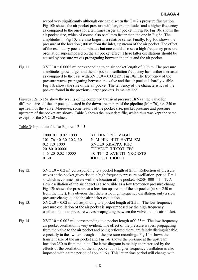
BILAGA 4

4-8

record very significantly although one can discern the T = 2 s pressure fluctuation. Fig 10b shows the air pocket pressure with larger amplitudes and a higher frequency as compared to the ones for a ten times larger air pocket in Fig 8b. Fig 10c shows the air pocket size, which of course also oscillates faster than the one in Fig 8c. The amplitudes in Fig 10c are also larger in a relative sense. Finally, Fig 10d shows the pressure at the location (300 m from the inlet) upstream of the air pocket. The effect of the oscillatory pocket dominates but one could also see a high frequency pressure oscillation superimposed on the air pocket effect. These latter oscillations should be caused by pressure waves propagating between the inlet and the air pocket.

Fig 11. XVOL0 = 0.0005 m3 corresponding to an air pocket length of 0.06 m. The pressure

amplitudes grow larger and the air pocket oscillation frequency has further increased as compared to the case with XVOL0 = 0.002 m3, Fig 10a. The frequency of the pressure waves propagating between the valve and the air pocket is hardly visible. Fig 11b shows the size of the air pocket. The tendency of the characteristics of the pocket, found in the previous, larger pockets, is maintained.

Figures 12a to 15a show the results of the computed transient pressure H(N) at the valve for different sizes of the air pocket located in the downstream part of the pipeline (M = 76), i.e. 250 m upstream of the valve. Moreover, some results of the pocket size, pocket pressure and pressure upstream of the pocket are shown. Table 3 shows the input data file, which thus was kept the same except for the XVOL0 values. Table 3: Input data file for Figures 12–15

1000 0.1 0.02 1000 XL DIA FRIK VAGH 101 76 40 30 10.2 30 N M HIN HUT HATM ZM 0.2 1.0 1000 XVOL0 XKAPPA RHO 20 80 0.00001 TIDVENT TIDTOT EPS 1 5 20 0.02 10000 T0 T1 T2 XVENT1 XKONST0 0 30 IOUTPUT IHOUT1

Fig 12. XVOL0 = 0.2 m3 corresponding to a pocket length of 25 m. Reflection of pressure

waves at the pocket gives rise to a high frequency pressure oscillation, period T = 1 s, which is commensurate with the location of the pocket: 4·250/1000 = 1 = T. A slow oscillation of the air pocket is also visible as a low frequency pressure change. Fig 12b shows the pressure at a location upstream of the air pocket (at x = 250 m from the inlet). It is obvious that there is no high frequency oscillation, only a slow pressure change due to the air pocket oscillation.

Fig 13. XVOL0 = 0.02 m3 corresponding to a pocket length of 2.5 m. The low frequency pressure oscillation of the air pocket is superimposed by the high frequency oscillation due to pressure waves propagating between the valve and the air pocket.

Fig 14. XVOL0 = 0.002 m3, corresponding to a pocket length of 0.25 m. The low frequency

air pocket oscillation is very evident. The effect of the pressure waves, propagating from the valve to the air pocket and being reflected there, are faintly distinguishable, especially in the “wider” troughs of the pressure recording.. Fig 14b shows the transient size of the air pocket and Fig 14c shows the pressure at the upstream location 250 m from the inlet. The latter diagram is mainly characterized by the effects of the oscillation of the air pocket but a higher frequency oscillation is also imposed with a time period of about 1.6 s. This latter time period will change with

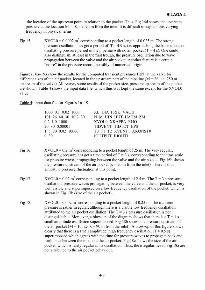
BILAGA 4

4-9

the location of the upstream point in relation to the pocket. Thus, Fig 14d shows the upstream pressure at the location M = 10, i.e. 90 m from the inlet. It is difficult to explain this varying frequency in physical terms.

Fig 15. XVOL0 = 0.0002 m3 corresponding to a pocket length of 0.025 m. The strong

pressure oscillation has got a period of T ≈ 4.9 s, i.e. approaching the basic transient oscillating pressure period in the pipeline with no air pocket (T = 4 s). One could also distinguish, at least in the first trough, the pressure oscillation due to wave propagation between the valve and the air pocket. Another feature is a certain “noise” in the pressure record, possibly of numerical origin.

Figures 16a–19a show the results for the computed transient pressures H(N) at the valve for different sizes of the air pocket, located in the upstream part of the pipeline (M = 26, i.e. 750 m upstream of the valve). Moreover, some results of the pocket size, pressure upstream of the pocket are shown. Table 4 shows the input data file, which thus was kept the same except for the XVOL0 value. Table 4: Input data file for Figures 16–19

1000 0.1 0.02 1000 XL DIA FRIK VAGH 101 26 40 30 10.2 30 N M HIN HUT HATM ZM 0.2 1.0 1000 XVOL0 XKAPPA RHO 20 80 0.00001 TIDVENT TIDTOT EPS 1 5 20 0.02 10000 T0 T1 T2 XVENT1 XKONST0 0 30 IOUTPUT IHOUT1

Fig 16. XVOL0 = 0.2 m3 corresponding to a pocket length of 25 m. The very regular,

oscillating pressure has got a time period of T = 3 s, corresponding to the time scale for pressure waves propagating between the valve and the air pocket. Fig 16b shows the pressure upstream of the air pocket (x = 90 m from the inlet). There is thus almost no pressure fluctuation at this point.

Fig 17. XVOL0 = 0.02 m3 corresponding to a pocket length of 2.5 m. The T = 3 s pressure

oscillation, pressure waves propagating between the valve and the air pocket, is very well visible and superimposed on a low frequency oscillation of the pocket, which is shown in Fig 17b (size of the air pocket).

Fig 18. XVOL0 = 0.002 m3 corresponding to a pocket length of 0.25 m. The transient

pressure is rather irregular, although there is a visible low frequency oscillation attributed to the air pocket oscillation. The T = 3 s pressure oscillation is not distinguishable. Moreover, a blow-up of the diagram shows that there is a T = 1 s small amplitude oscillation superimposed. Fig 18b shows the pressure upstream of the air pocket (M = 10, i.e. x = 90 m from the inlet). A blow-up of this figure shows clearly that there is a small amplitude, high frequency oscillation (T ≈ 0.5 s) superimposed which agrees with the time for pressure waves to propagate back and forth once between the inlet and the air pocket. Fig 18c shows the size of the air pocket, which is fairly regular in its oscillation. Thus, the irregularities in Fig 18a are not attributed to the air pocket behaviour.

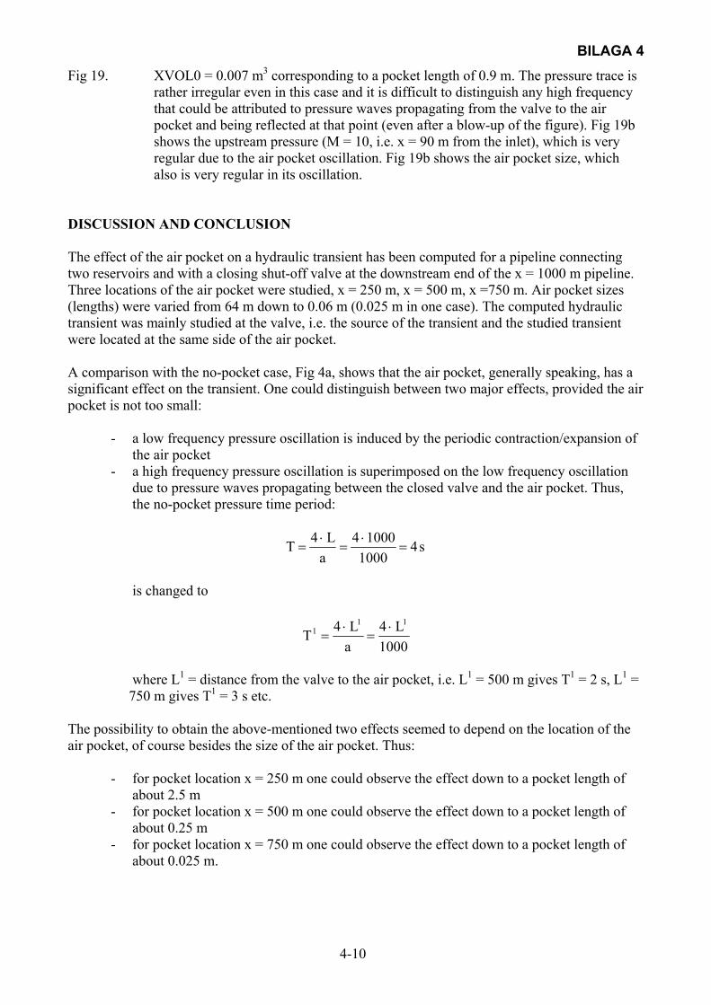
BILAGA 4

4-10

Fig 19. XVOL0 = 0.007 m3 corresponding to a pocket length of 0.9 m. The pressure trace is rather irregular even in this case and it is difficult to distinguish any high frequency that could be attributed to pressure waves propagating from the valve to the air pocket and being reflected at that point (even after a blow-up of the figure). Fig 19b shows the upstream pressure (M = 10, i.e. x = 90 m from the inlet), which is very regular due to the air pocket oscillation. Fig 19b shows the air pocket size, which also is very regular in its oscillation.

DISCUSSION AND CONCLUSION The effect of the air pocket on a hydraulic transient has been computed for a pipeline connecting two reservoirs and with a closing shut-off valve at the downstream end of the x = 1000 m pipeline. Three locations of the air pocket were studied, x = 250 m, x = 500 m, x =750 m. Air pocket sizes (lengths) were varied from 64 m down to 0.06 m (0.025 m in one case). The computed hydraulic transient was mainly studied at the valve, i.e. the source of the transient and the studied transient were located at the same side of the air pocket. A comparison with the no-pocket case, Fig 4a, shows that the air pocket, generally speaking, has a significant effect on the transient. One could distinguish between two major effects, provided the air pocket is not too small:

- a low frequency pressure oscillation is induced by the periodic contraction/expansion of the air pocket

- a high frequency pressure oscillation is superimposed on the low frequency oscillation due to pressure waves propagating between the closed valve and the air pocket. Thus, the no-pocket pressure time period:

s41000

10004a

L4T =⋅

=⋅

=

is changed to

1000

L4aL4T

111 ⋅

=⋅

=

where L1 = distance from the valve to the air pocket, i.e. L1 = 500 m gives T1 = 2 s, L1 = 750 m gives T1 = 3 s etc.

The possibility to obtain the above-mentioned two effects seemed to depend on the location of the air pocket, of course besides the size of the air pocket. Thus:

- for pocket location x = 250 m one could observe the effect down to a pocket length of about 2.5 m

- for pocket location x = 500 m one could observe the effect down to a pocket length of about 0.25 m

- for pocket location x = 750 m one could observe the effect down to a pocket length of about 0.025 m.

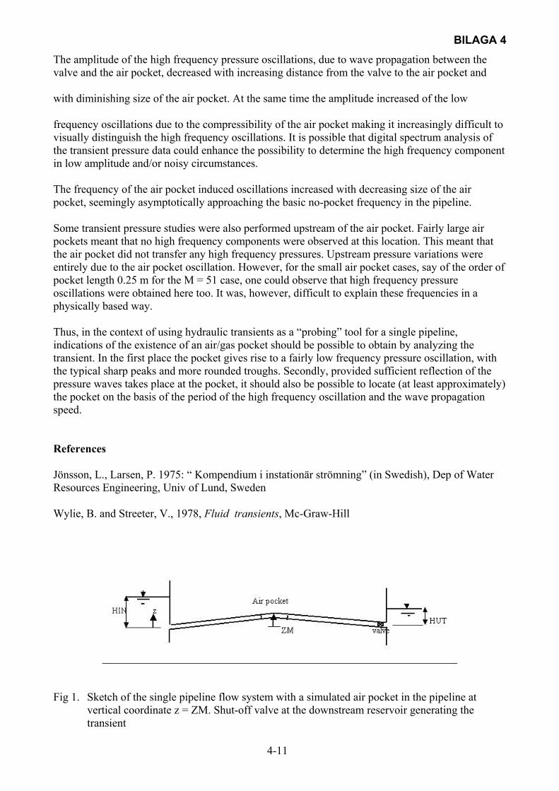
BILAGA 4

4-11

The amplitude of the high frequency pressure oscillations, due to wave propagation between the valve and the air pocket, decreased with increasing distance from the valve to the air pocket and with diminishing size of the air pocket. At the same time the amplitude increased of the low frequency oscillations due to the compressibility of the air pocket making it increasingly difficult to visually distinguish the high frequency oscillations. It is possible that digital spectrum analysis of the transient pressure data could enhance the possibility to determine the high frequency component in low amplitude and/or noisy circumstances. The frequency of the air pocket induced oscillations increased with decreasing size of the air pocket, seemingly asymptotically approaching the basic no-pocket frequency in the pipeline. Some transient pressure studies were also performed upstream of the air pocket. Fairly large air pockets meant that no high frequency components were observed at this location. This meant that the air pocket did not transfer any high frequency pressures. Upstream pressure variations were entirely due to the air pocket oscillation. However, for the small air pocket cases, say of the order of pocket length 0.25 m for the M = 51 case, one could observe that high frequency pressure oscillations were obtained here too. It was, however, difficult to explain these frequencies in a physically based way. Thus, in the context of using hydraulic transients as a “probing” tool for a single pipeline, indications of the existence of an air/gas pocket should be possible to obtain by analyzing the transient. In the first place the pocket gives rise to a fairly low frequency pressure oscillation, with the typical sharp peaks and more rounded troughs. Secondly, provided sufficient reflection of the pressure waves takes place at the pocket, it should also be possible to locate (at least approximately) the pocket on the basis of the period of the high frequency oscillation and the wave propagation speed. References Jönsson, L., Larsen, P. 1975: “ Kompendium i instationär strömning” (in Swedish), Dep of Water Resources Engineering, Univ of Lund, Sweden Wylie, B. and Streeter, V., 1978, Fluid transients, Mc-Graw-Hill

Fig 1. Sketch of the single pipeline flow system with a simulated air pocket in the pipeline at

vertical coordinate z = ZM. Shut-off valve at the downstream reservoir generating the transient

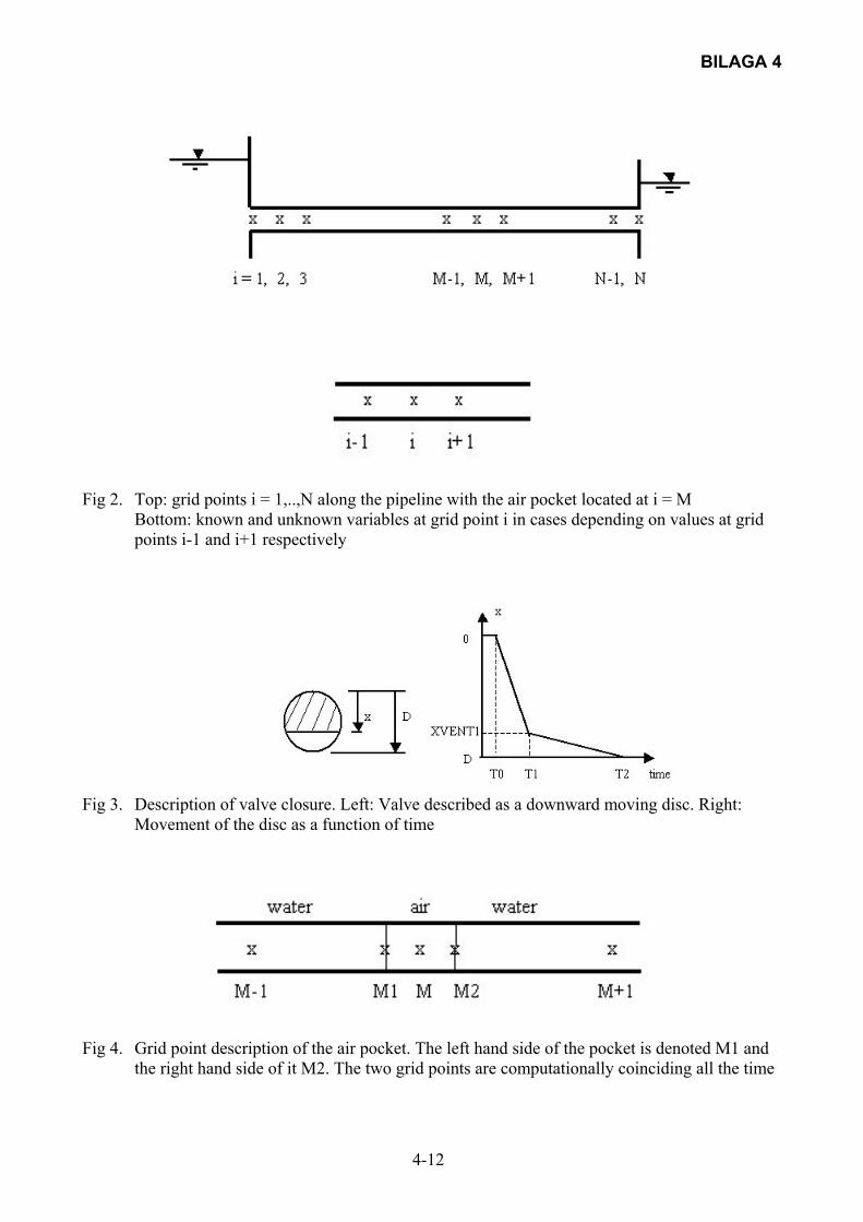
BILAGA 4

4-12

Fig 2. Top: grid points i = 1,..,N along the pipeline with the air pocket located at i = M

Bottom: known and unknown variables at grid point i in cases depending on values at grid points i-1 and i+1 respectively

Fig 3. Description of valve closure. Left: Valve described as a downward moving disc. Right:

Movement of the disc as a function of time

Fig 4. Grid point description of the air pocket. The left hand side of the pocket is denoted M1 and

the right hand side of it M2. The two grid points are computationally coinciding all the time

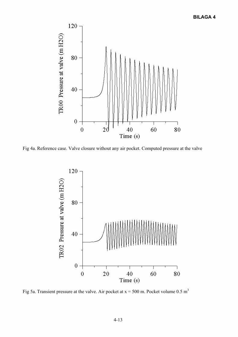
BILAGA 4

4-13

Fig 4a. Reference case. Valve closure without any air pocket. Computed pressure at the valve

Fig 5a. Transient pressure at the valve. Air pocket at x = 500 m. Pocket volume 0.5 m3

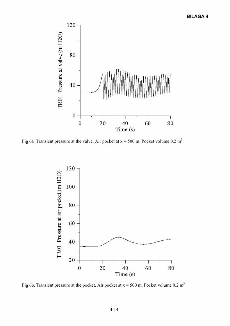
BILAGA 4

4-14

Fig 6a. Transient pressure at the valve. Air pocket at x = 500 m. Pocket volume 0.2 m3

Fig 6b. Transient pressure at the pocket. Air pocket at x = 500 m. Pocket volume 0.2 m3

BILAGA 4

4-15

Fig 6c. Air pocket volume. Air pocket at x = 500 m. Pocket volume 0.2 m3

Fig 6d. Pressure at upstream (x = 300 m) location. Air pocket location x = 500 m. Pocket volume 0.2 m3

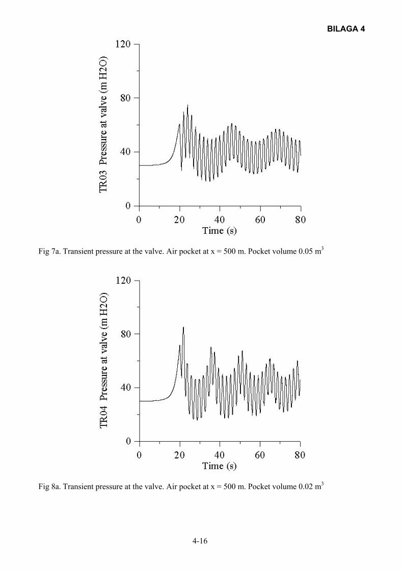
BILAGA 4

4-16

Fig 7a. Transient pressure at the valve. Air pocket at x = 500 m. Pocket volume 0.05 m3

Fig 8a. Transient pressure at the valve. Air pocket at x = 500 m. Pocket volume 0.02 m3

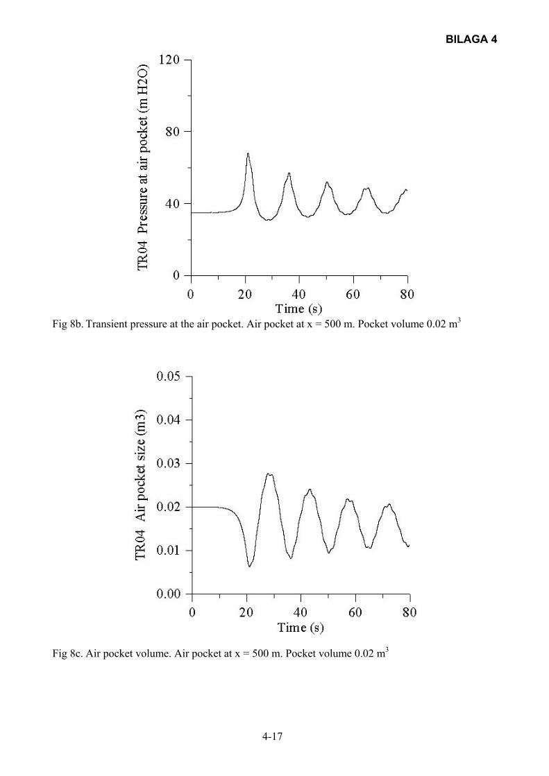
BILAGA 4

4-17

Fig 8b. Transient pressure at the air pocket. Air pocket at x = 500 m. Pocket volume 0.02 m3

Fig 8c. Air pocket volume. Air pocket at x = 500 m. Pocket volume 0.02 m3

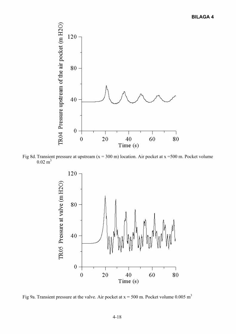
BILAGA 4

4-18

Fig 8d. Transient pressure at upstream (x = 300 m) location. Air pocket at x =500 m. Pocket volume

0.02 m3

Fig 9a. Transient pressure at the valve. Air pocket at x = 500 m. Pocket volume 0.005 m3

BILAGA 4

4-19

Fig 10a. Transient pressure at the valve. Air pocket at x = 500 m. Pocket volume 0.002 m3

Fig 10b. Transient pressure at the pocket. Air pocket at x = 500 m. Pocket volume 0.002 m3

BILAGA 4

4-20

Fig 10c. Air pocket volume. Air pocket at x = 500 m. Pocket volume 0.002 m3

Fig 10d. Transient pressure at an upstream (x = 300 m) location. Air pocket at x = 500 m. Pocket volume 0.002 m3

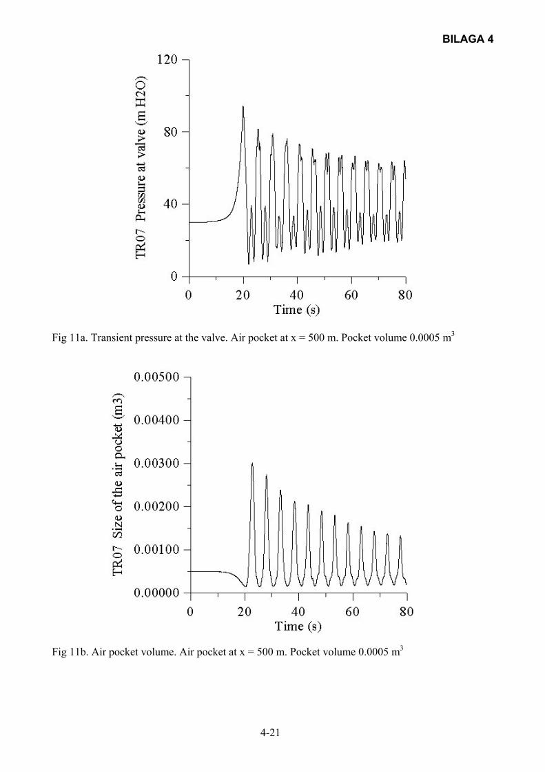
BILAGA 4

4-21

Fig 11a. Transient pressure at the valve. Air pocket at x = 500 m. Pocket volume 0.0005 m3

Fig 11b. Air pocket volume. Air pocket at x = 500 m. Pocket volume 0.0005 m3

BILAGA 4

4-22

Fig 12a. Transient pressure at the valve. Air pocket at x = 750 m. Pocket volume 0.2 m3

Fig 12b. Transient pressure at an upstream (x = 250 m) location. Air pocket at x = 750 m. Pocket volume 0.2 m3

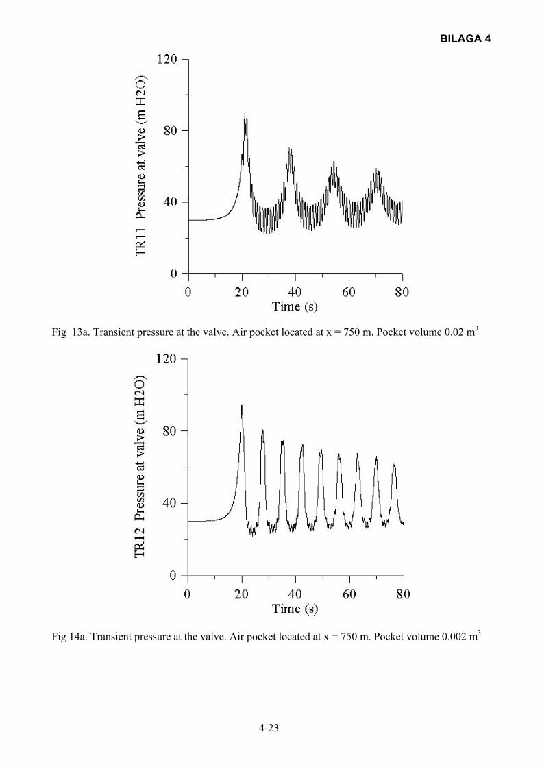
BILAGA 4

4-23

Fig 13a. Transient pressure at the valve. Air pocket located at x = 750 m. Pocket volume 0.02 m3

Fig 14a. Transient pressure at the valve. Air pocket located at x = 750 m. Pocket volume 0.002 m3

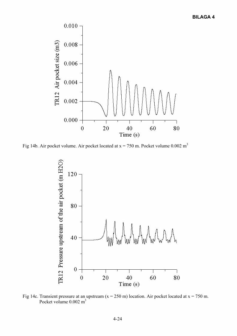
BILAGA 4

4-24

Fig 14b. Air pocket volume. Air pocket located at x = 750 m. Pocket volume 0.002 m3

Fig 14c. Transient pressure at an upstream (x = 250 m) location. Air pocket located at x = 750 m. Pocket volume 0.002 m3

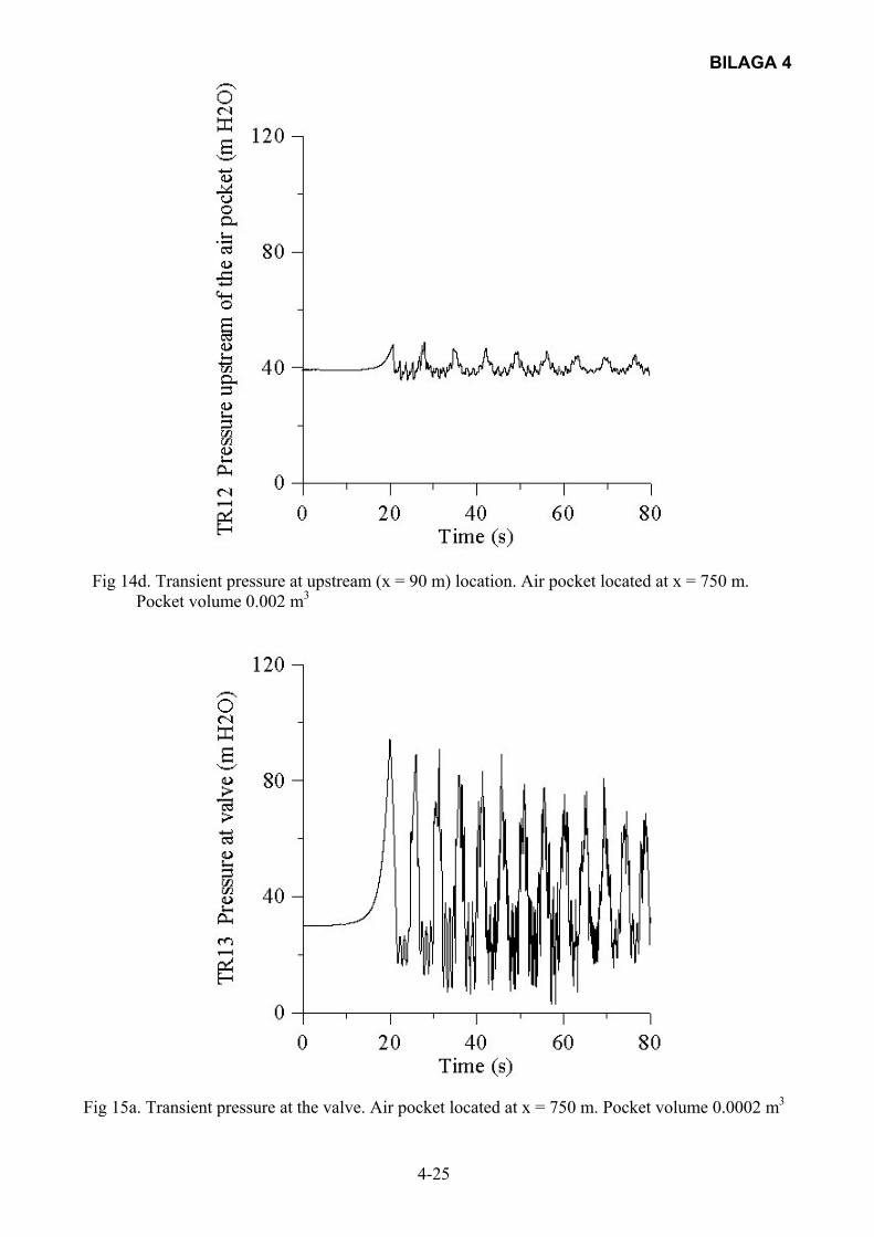
BILAGA 4

4-25

Fig 14d. Transient pressure at upstream (x = 90 m) location. Air pocket located at x = 750 m. Pocket volume 0.002 m3

Fig 15a. Transient pressure at the valve. Air pocket located at x = 750 m. Pocket volume 0.0002 m3

BILAGA 4

4-26

Fig 16a. Transient pressure at the valve. Air pocket located at x = 250 m. Pocket volume 0.2 m3

Fig 16b. Transient pressure at an upstream (x = 90 m) location. Air pocket volume located at x = 250 m. Pocket volume 0.2 m3

BILAGA 4

4-27

Fig 17a. Transient pressure at the valve. Air pocket located at x = 250 m. Pocket volume 0.02 m3

Fig 17b. Air pocket volume. Air pocket located at x = 250 m. Pocket volume 0.02 m3

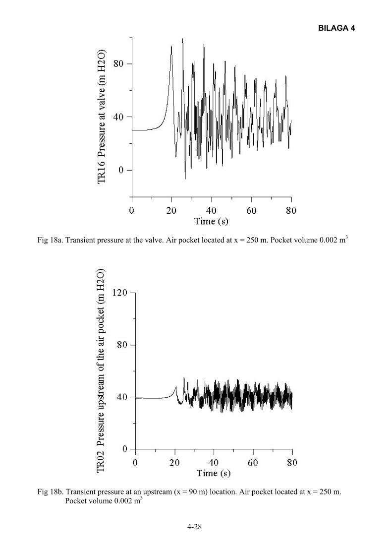
BILAGA 4

4-28

Fig 18a. Transient pressure at the valve. Air pocket located at x = 250 m. Pocket volume 0.002 m3

Fig 18b. Transient pressure at an upstream (x = 90 m) location. Air pocket located at x = 250 m. Pocket volume 0.002 m3

BILAGA 4

4-29

Fig 18c. Air pocket volume. Air pocket located at x = 250 m. Pocket volume 0.002 m3

Fig 19a. Transient pressure at the valve. Air pocket located at x = 250 m. Pocket volume 0.007 m3

BILAGA 4

4-30

Fig 19b. Transient pressure at upstream (x = 90 m) location. Air pocket located at x = 250 m. Pocket volume 0.007 m3

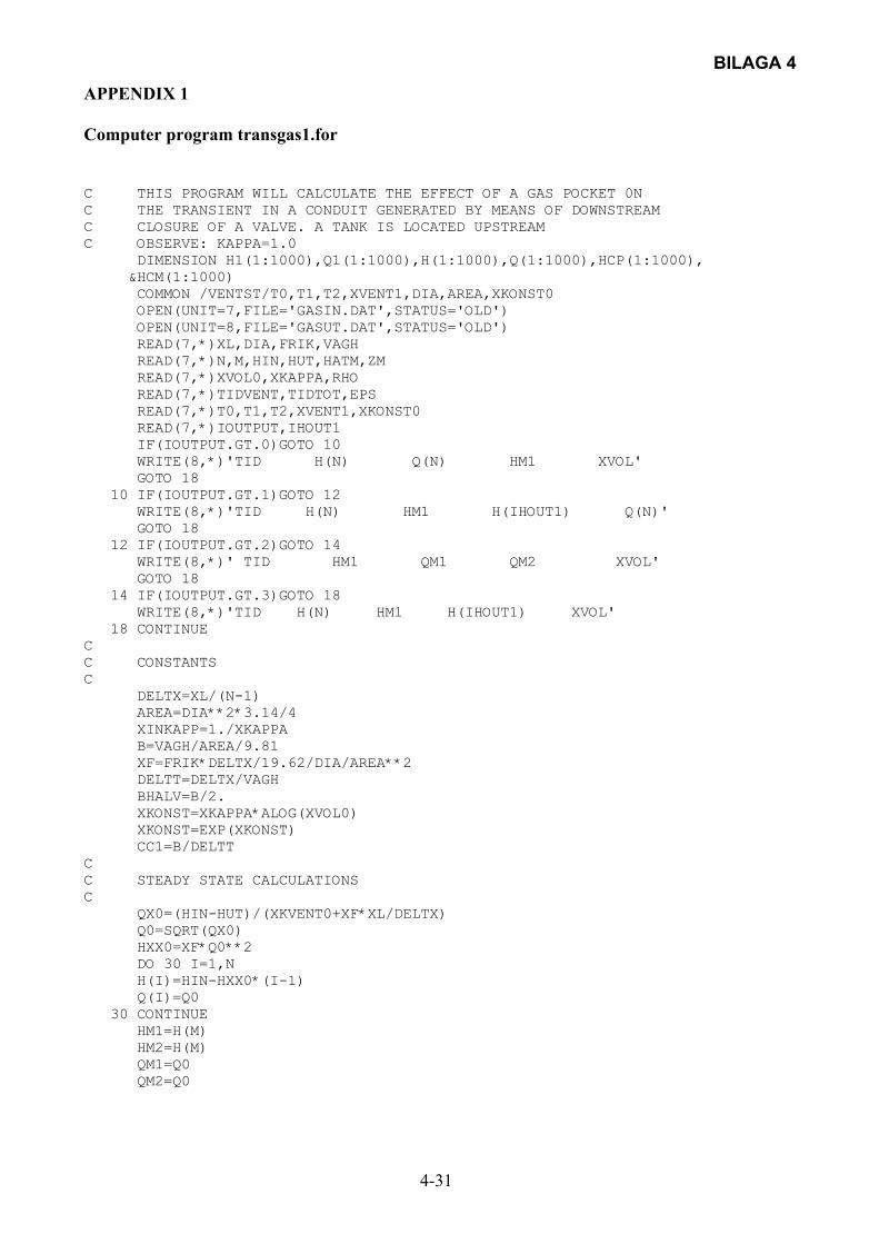
BILAGA 4

4-31

APPENDIX 1 Computer program transgas1.for C THIS PROGRAM WILL CALCULATE THE EFFECT OF A GAS POCKET 0N C THE TRANSIENT IN A CONDUIT GENERATED BY MEANS OF DOWNSTREAM C CLOSURE OF A VALVE. A TANK IS LOCATED UPSTREAM C OBSERVE: KAPPA=1.0 DIMENSION H1(1:1000),Q1(1:1000),H(1:1000),Q(1:1000),HCP(1:1000), &HCM(1:1000) COMMON /VENTST/T0,T1,T2,XVENT1,DIA,AREA,XKONST0 OPEN(UNIT=7,FILE='GASIN.DAT',STATUS='OLD') OPEN(UNIT=8,FILE='GASUT.DAT',STATUS='OLD') READ(7,*)XL,DIA,FRIK,VAGH READ(7,*)N,M,HIN,HUT,HATM,ZM READ(7,*)XVOL0,XKAPPA,RHO READ(7,*)TIDVENT,TIDTOT,EPS READ(7,*)T0,T1,T2,XVENT1,XKONST0 READ(7,*)IOUTPUT,IHOUT1 IF(IOUTPUT.GT.0)GOTO 10 WRITE(8,*)'TID H(N) Q(N) HM1 XVOL' GOTO 18 10 IF(IOUTPUT.GT.1)GOTO 12 WRITE(8,*)'TID H(N) HM1 H(IHOUT1) Q(N)' GOTO 18 12 IF(IOUTPUT.GT.2)GOTO 14 WRITE(8,*)' TID HM1 QM1 QM2 XVOL' GOTO 18 14 IF(IOUTPUT.GT.3)GOTO 18 WRITE(8,*)'TID H(N) HM1 H(IHOUT1) XVOL' 18 CONTINUE C C CONSTANTS C DELTX=XL/(N-1) AREA=DIA**2*3.14/4 XINKAPP=1./XKAPPA B=VAGH/AREA/9.81 XF=FRIK*DELTX/19.62/DIA/AREA**2 DELTT=DELTX/VAGH BHALV=B/2. XKONST=XKAPPA*ALOG(XVOL0) XKONST=EXP(XKONST) CC1=B/DELTT C C STEADY STATE CALCULATIONS C QX0=(HIN-HUT)/(XKVENT0+XF*XL/DELTX) Q0=SQRT(QX0) HXX0=XF*Q0**2 DO 30 I=1,N H(I)=HIN-HXX0*(I-1) Q(I)=Q0 30 CONTINUE HM1=H(M) HM2=H(M) QM1=Q0 QM2=Q0

BILAGA 4

4-32

P0ZM=(H(M)-ZM+HATM)*RHO*9.81 XKONST=XKONST*P0ZM CC2=XINKAPP*ALOG(XKONST/RHO/9.81) CC2=EXP(CC2) C2=CC1*CC2 TID=0 XVOL=XVOL0 C C START OF ITERATIVE PROCEDURE, CALCULATION OF HCP, HCM C 700 DO 50 I=1,M-1 YYA=B*Q(I) YYB=XF*Q(I)*ABS(Q(I)) HCP(I)=H(I)+YYA-YYB HCM(I)=H(I)-YYA+YYB 50 CONTINUE HCPM2=HM2+B*QM2-XF*QM2*ABS(QM2) HCMM1=HM1-B*QM1+XF*QM1*ABS(QM1) DO 60 I=M+1,N YYA=B*Q(I) YYB=XF*Q(I)*ABS(Q(I)) HCP(I)=H(I)+YYA-YYB HCM(I)=H(I)-YYA+YYB 60 CONTINUE C C INNER POINTS C DO 100 I=2,M-2 H1(I)=(HCP(I-1)+HCM(I+1))*0.5 Q1(I)=(H1(I)-HCM(I+1))/B 100 CONTINUE DO 110 I=M+2,N-1 H1(I)=(HCP(I-1)+HCM(I+1))*0.5 Q1(I)=(H1(I)-HCM(I+1))/B 110 CONTINUE H1(M-1)=(HCP(M-2)+HCMM1)*0.5 Q1(M-1)=(HCP(M-2)-H1(M-1))/B H1(M+1)=(HCPM2+HCM(M+2))*0.5 Q1(M+1)=(H1(M+1)-HCM(M+2))/B C C BOUNDARY POINTS C C INLET C H1(1)=HIN Q1(1)=(H1(1)-HCM(2))/B C C VALVE C IF(TID.GE.TIDVENT-0.0000001)GOTO 230 CALL XKV(TID,XKVENT) XX1=B/2/XKVENT XX2=(HCP(N-1)-HUT)/XKVENT IF(XX2.GT.0.0000000001)GOTO 200 IF(XX2.LT.-0.000000001)GOTO 210 Q1(N)=0 GOTO 220 200 Q1(N)=-XX1+SQRT(XX1**2+XX2) GOTO 220 210 Q1(N)=XX1-SQRT(XX1**2-XX2) GOTO 220 220 CONTINUE H1(N)=HCP(N-1)-B*Q1(N)

BILAGA 4

4-33

GOTO 240 230 Q1(N)=0 H1(N)=HCP(N-1) 240 CONTINUE C C GAS POCKET, KAPPA=1 C C1=0.5*(HCP(M-1)+HCM(M+1))-BHALV*(QM2-QM1)-CC1*XVOL ALFA1=ZM-HATM+C1 ALFA2=C2+C1*HATM-C1*ZM XLOESN1=ALFA1/2+SQRT((ALFA1/2)**2+ALFA2) XLOESN2=ALFA1/2-SQRT((ALFA1/2)**2+ALFA2) IF(XLOESN2.GT.XLOESN1)GOTO 314 H1M1=XLOESN1 H1M2=XLOESN1 GOTO 312 314 H1M1=XLOESN2 H1M2=XLOESN2 312 CONTINUE Q1M1=(HCP(M-1)-H1M1)/B Q1M2=(H1M2-HCM(M+1))/B XXVOL=XKONST/(H1M1-ZM+HATM)/RHO/9.81 WRITE(*,*)'XXVOL=',XXVOL XXVOL=XINKAPP*ALOG(XXVOL) XXVOL=EXP(XXVOL) X1VOL=XXVOL C C TRANSFER H1 TO H, Q1 TO Q ETC C DO 400 I=1,M-1 H(I)=H1(I) Q(I)=Q1(I) 400 CONTINUE DO 410 I=M+1,N H(I)=H1(I) Q(I)=Q1(I) 410 CONTINUE HM1=H1M1 HM2=H1M2 QM1=Q1M1 QM2=Q1M2 XVOL=X1VOL C C WRITE ON OUTPUT FILES C IF(IOUTPUT.GT.0)GOTO 510 WRITE(8,591)TID,H(N),Q(N),HM1,XVOL GOTO 590 510 IF(IOUTPUT.GT.1)GOTO 520 WRITE(8,592)TID,H(N),HM1,H(IHOUT1),Q(N) GOTO 590 520 IF(IOUTPUT.GT.2)GOTO 530 WRITE(8,593)TID,HM1,QM1,QM2,XVOL GOTO 590 530 IF(IOUTPUT.GT.3)GOTO 590 WRITE(8,*)TID,H(N),HM1,H(IHOUT1),XVOL 590 CONTINUE

BILAGA 4

4-34

TID=TID+DELTT IF(TID.LT.TIDTOT)GOTO 700 591 FORMAT(F7.3,3X,F6.2,3X,F9.6,3X,F6.2,3X,F12.9) 592 FORMAT(F7.3,3X,F6.2,3X,F6.2,4X,F6.2,8X,F9.6) 593 FORMAT(F7.3,3X,F6.2,3X,F9.6,3X,F9.6,3X,F12.9) 599 CONTINUE END C C SUBROUTINE XKV C SUBROUTINE XKV(TIME,XKVV) COMMON /VENTST/T0,T1,T2,XVENT1,DIA,AREA,XKONST0 IF(TIME.GT.T0)GOTO 600 XKVV=0.001 GOTO 620 600 CONTINUE IF(TIME.GT.T1)GOTO 610 XLAGE=XVENT1*(TIME-T0)/(T1-T0) AOPP=(DIA-XLAGE)/DIA*AREA XKVV=(1-AREA/AOPP)**2*XKONST0 GOTO 620 610 CONTINUE XLAGE=XVENT1+(DIA-XVENT1)*(TIME-T1)/(T2-T1) AOPP=(DIA-XLAGE)/DIA*AREA XKVV=(1-AREA/AOPP)**2*XKONST0 620 CONTINUE RETURN END

BILAGA 5

DEPARTMENT OF WATER RESOURCES ENGINEERING LUND INSTITUTE OF TECHNOLOGY, LUND UNIVERSITY

CODEN:LUTVDG/(TVVR-3241)/1-49(2003)

MEASUREMENTS OF HYDRAULIC TRANSIENTS IN SEWAGE WATER PUMPING STATIONS – ANALYSIS, WAVE PROPAGATION VELOCITIES

by

Lennart Jönsson

The research reported in this document has been made possible through the sponsorship by Ångpanneföreningens Forskningsstiftelse, Stockholm, Sweden and by VA-Forsk, Stockholm,

Sweden

BILAGA 5

CONTENTS page Abstract......................................................................................................... 5-1 Acknowledgement ........................................................................................ 5-1 Introduction .................................................................................................. 5-2 Measurement equipment .............................................................................. 5-2 Measurement locations................................................................................. 5-2 Yndesäte pumping station ............................................................................ 5-3 Vallåkra pumping station.............................................................................. 5-6 Espet pumping station .................................................................................. 5-9 Golfbanan pumping station ........................................................................ 5-11 Södervidinge pumping station.................................................................... 5-12 Hög pumping station .................................................................................. 5-14 Skarviken pumping station ......................................................................... 5-15 Vallösa pumping station ............................................................................. 5-17 Kristinedal pumping station ....................................................................... 5-20 Discussion................................................................................................... 5-22 References .................................................................................................. 5-23 Figures/Diagrams 1–50 .............................................................................. 5-24

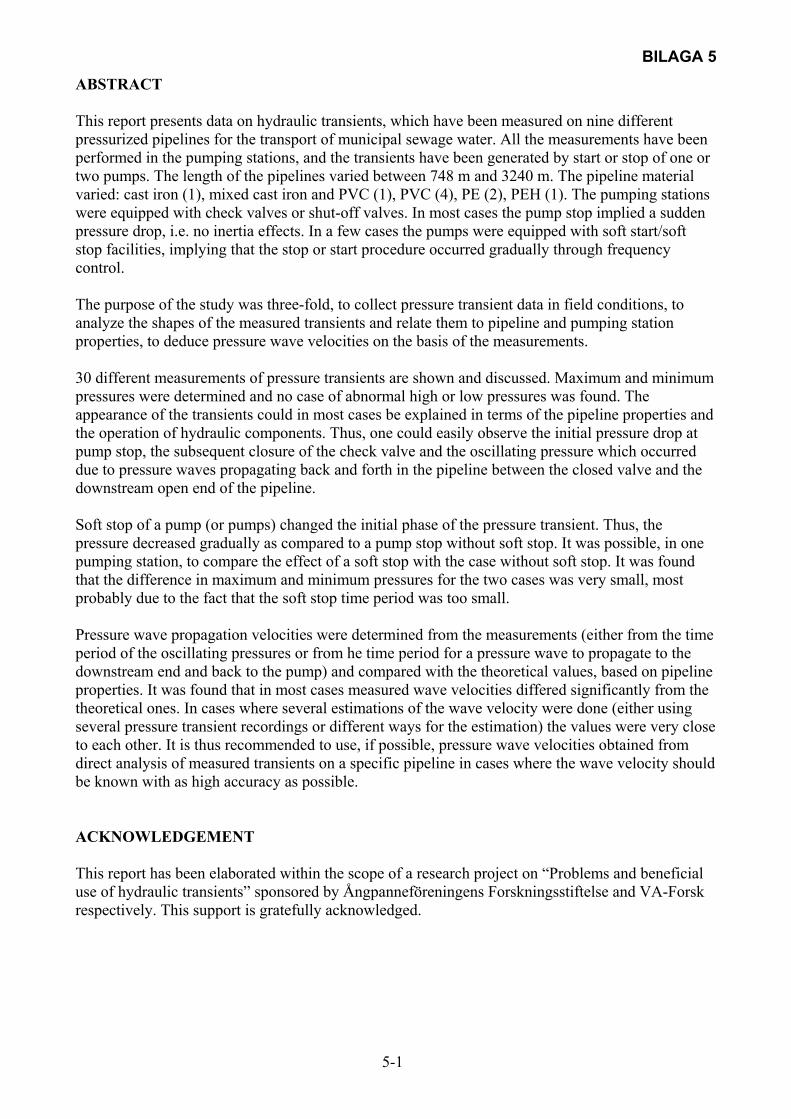
BILAGA 5

5-1

ABSTRACT This report presents data on hydraulic transients, which have been measured on nine different pressurized pipelines for the transport of municipal sewage water. All the measurements have been performed in the pumping stations, and the transients have been generated by start or stop of one or two pumps. The length of the pipelines varied between 748 m and 3240 m. The pipeline material varied: cast iron (1), mixed cast iron and PVC (1), PVC (4), PE (2), PEH (1). The pumping stations were equipped with check valves or shut-off valves. In most cases the pump stop implied a sudden pressure drop, i.e. no inertia effects. In a few cases the pumps were equipped with soft start/soft stop facilities, implying that the stop or start procedure occurred gradually through frequency control. The purpose of the study was three-fold, to collect pressure transient data in field conditions, to analyze the shapes of the measured transients and relate them to pipeline and pumping station properties, to deduce pressure wave velocities on the basis of the measurements. 30 different measurements of pressure transients are shown and discussed. Maximum and minimum pressures were determined and no case of abnormal high or low pressures was found. The appearance of the transients could in most cases be explained in terms of the pipeline properties and the operation of hydraulic components. Thus, one could easily observe the initial pressure drop at pump stop, the subsequent closure of the check valve and the oscillating pressure which occurred due to pressure waves propagating back and forth in the pipeline between the closed valve and the downstream open end of the pipeline. Soft stop of a pump (or pumps) changed the initial phase of the pressure transient. Thus, the pressure decreased gradually as compared to a pump stop without soft stop. It was possible, in one pumping station, to compare the effect of a soft stop with the case without soft stop. It was found that the difference in maximum and minimum pressures for the two cases was very small, most probably due to the fact that the soft stop time period was too small. Pressure wave propagation velocities were determined from the measurements (either from the time period of the oscillating pressures or from he time period for a pressure wave to propagate to the downstream end and back to the pump) and compared with the theoretical values, based on pipeline properties. It was found that in most cases measured wave velocities differed significantly from the theoretical ones. In cases where several estimations of the wave velocity were done (either using several pressure transient recordings or different ways for the estimation) the values were very close to each other. It is thus recommended to use, if possible, pressure wave velocities obtained from direct analysis of measured transients on a specific pipeline in cases where the wave velocity should be known with as high accuracy as possible. ACKNOWLEDGEMENT This report has been elaborated within the scope of a research project on “Problems and beneficial use of hydraulic transients” sponsored by Ångpanneföreningens Forskningsstiftelse and VA-Forsk respectively. This support is gratefully acknowledged.

BILAGA 5

5-2

INTRODUCTION Hydraulic transients or pressure transients occur in pressurized pipelines for water conveyance due to rapid flow changes, most often due to pump stop, pump start, valve operation, check valve closure. Such transients are characterized by more or less strong pressure changes, which propagate through the pipeline with the pressure wave velocity, normally in the range of a few 100:s of m/s for rather elastic pipes up to the theoretical limit of 1440 m/s in a completely rigid pipe. The unsteady pressure phase gives rise to high pressures, low pressures and oscillating pressures. Normally, a pressure transient is considered as a problem due to the potential risk for damages to the pipeline. However, one could also consider transients in a more positive way as the transients contain some information on the pipeline and the operation/function of hydraulic components. The purpose of this study is threefold:

- to collect pressure transient data in field conditions for some different kinds of pipelines (short/ long pipelines, different pipe materials, different pressure wave velocities, different hydraulic components etc). The measurements have been performed on a number of sewage water pumping stations.

- to analyze the shapes of the measured transients and to relate them to physical properties of the pipeline or to the function of hydraulic components

- to evaluate the pressure wave velocities from the measurements and to compare these velocities with theoretical wave velocities determined on the basis of existing knowledge of the specific pipelines. An accurate knowledge of the wave velocity is a prerequisite in many cases for using a transient as a “tool” for deriving information on some hydraulic properties of a pipeline.

MEASUREMENT EQUIPMENT The pressure transients were performed using a 10 bar dynamic pressure transducer, capable of measuring sub atmospheric pressures too (down to vacuum). Existing taps on the pipeline in the pumping stations were used for attaching the transducer to the pipe immediately downstream of the valve(s). The transducer was connected to a minicomputer (ABC80) with an accurate amplifier and a fast A/D converter. In this way digital pressure transient data could be obtained with a sample rate of up to 640 Hz although such a high rate was not required in the measurements (normally 25 Hz or 50 Hz were used for sample frequencies). The pressure transducer had previously been calibrated accurately and its linear calibration has been found to be very stable. The function of the pressure transducer was also tested at the different measurement occasions by measuring the atmospheric pressure and also by checking (measuring) the geometric heads at the different pumping stations. A more detailed description of the measurement equipment can be found in a previous report by the author (Jönsson 2002). MEASUREMENT LOCATIONS Eleven pumping stations in Skåne, mainly for municipal sewage water, were visited for pressure transient measurements. Results from nine of these stations are presented in this report. The pumping stations and the pipelines had different characteristics: Pipeline lengths: 748 m up to 3240 m Pipe materials: cast iron, PE, PEH, PVC, mixed cast iron/PVC

BILAGA 5

5-3

Valves: ball and swing check valves, shut-off valve Pump control: soft stop, soft start, ordinary stop and start (no inertia) Transient generation: stop/start for one pump, stop/start for two pumps in parallel, stop/start for two

pumps in series, stop/start with check valve, shut-off valve closure/opening before pump stop/start, pump stop without shut-off valve closure.

Relevant data about the pipelines and the pumping stations were (as far as possible) collected from the water and sewage works in the different municipalities. In several cases the pump characteristics was obtained by contacting representatives of the pump manufacturers directly. As a complement to pipeline profile drawings, the geometric heads were also checked against the pressure measurements (both steady state and transient phases were utilized). Steady state flows were in most cases derived from pump diagrams and inferred pump heads (the latter obtained from the measurements and information about the geometry of the pumping stations). In a few cases, the pumping stations were equipped with flow meters. The pressure transient measurements were analyzed in different ways, such as:

- pressure wave velocities were mainly derived from the oscillating pressure time period using the average for a number of oscillations and a careful analysis of the digital data base, sample by sample to find out the time for the different pressure peaks. In some cases it was also possible to derive a wave velocity from the assumed propagation time, initially at pump stop, for a pressure wave from the pump to the downstream end of the pipeline and back to the pump. Theoretical pressure wave velocities were calculated on the basis of the well known formula for thin-walled pipes and assuming axial rigidity of the pipeline

- pressure drops at instantaneous pump stop were studied in relation to the location of the transducer, the pump sump water level, the wave velocity, the steady state water velocity

- maximum and minimum pressure levels were determined for the transient phases - indications of cavitation in pipeline and its possible relation to the pipeline profile - the effect of soft stop compared to an instantaneous stop - other specific characteristics

YNDESÄTE PUMPING STATION Yndesäte sewage water pumping station is located in the Helsingborg municipality and pumps sewage water to the next pumping station, Påarp Östra. The pressurized pipeline profile is described by the following horizontal and vertical coordinates starting at the pumping station: Length from Vertical coordinate pumping stn (m) (m)

0 45.80 184 48.00 323 48.60 494 48.95 681 54.40 763 55.30

The profile is thus rising continuously without any local peaks. Relevant data for the pumping station and the pipeline:

BILAGA 5

5-4

Pumps: CP3200-610, Flygt (two in parallel). The pump curve is shown in Fig 1 Valve: Swing check valve Pump sump water level: 41.8 m Geometric head: 13.5 m Pipeline length: 763 m Pipe material: Cast iron, diameter 250 mm, wall thickness 8–10 mm The pressure transducer was attached to the pressure side of the pipeline and immediately after the check valve. The vertical location of the transducer was about 3.8 m above the pump sump water level. Four different transient measurements were performed, YNDE01, YNDE02, YNDE03, YNDE04. The pressure transducer measured a pressure of 19.3 m (absolute pressure) when no pump was running. This means that the geometric head for the pumps would amount to: 19.3 - 10.2 + 3.8 = 12.9 m which is in good agreement with data from the profile drawing and the pump sump level (13.5 m). Measurements: YNDE01, shown in Fig 2. One pump running and stop of the pump. Sample rate 50 Hz, measurement time 50 s. Steady state pressure in the measurement point about 26 m implying a total pump head of 19.6 m (geometric head + friction) implying a flow of 50 l/s. The measured maximum pressure amounts to 34.4 m absolute pressure and the measured minimum pressure to 6.2 m absolute pressure. The pressure drops immediately to a pressure below the atmospheric pressure (10.2 m) due to the location of the measurement point and head loss in the passively rotating pump after pump stop (no inertia). When the flow at the check valve tends to reverse the check valve closes almost instantaneously and the pressure rises. After that one obtains the typical oscillating pressure due to pressure waves propagating back and forth through the entire pipeline between the closed check valve and the downstream end of the pipeline. The average value of the oscillatory pressure time period was found to be about T = 3.27 s which gives a pressure wave velocity a = 932 m/s according to the equation:

aL4T ⋅

= (1)

where L = length of the pipeline a = pressure wave velocity T = time period of pressure oscillations. The measured pressure wave propagation value should be compared with the theoretical one according to the expression:

const

eD

EE1

E

a

pipe

O2H

O2H

O2H

theor

⋅⋅+

ρ= (2)

BILAGA 5

5-5

where EH2O = modulus of elasticity for water (N/m2) Epipe = modulus of elasticity for the pipe material (N/m2) ρH2O = density of water (kg/m3) D = pipe diameter (inner) (m) e = pipe wall thickness (m)

const related to the axial behaviour of the pipeline, set to 1 – µ2 assuming no axial movement (µ = Poisson’s constant)

Using Epipe = 100·109 N/m2 for cast iron, EH2O = 2.1·109 N/m2 for water, D = 0.25 m, e = 0.009 m, ρH2O = 1000 kg/m3 one obtains: atheor = 1150 m/s which is considerably higher than the measured one. One possible reason for the deviation might be given by the fact that sewage water is pumped. In such a case there is a possibility for the existence of tiny gas bubbles in the pipeline, reducing the wave speed. Fig 2 also shows that there are some small disturbances on the pressure trace after valve closure. The reason for this fact is not obvious. The disturbances do not seem to be sufficiently irregular to be related to cavitation. Moreover, there is no reason for cavitation to occur for this kind of pipeline profile. One possible reason might be given by some subsequent movement of the check valve. YNDE01, enhancement, shown in Fig 3. Fig 3 shows an enlargement of the initial transient pressure phase. The valve closes at about t = 15.5 s after which the pressure oscillation takes place as depicted in Fig 2. One can also notice the disturbances on the pressure trace after valve closure. These disturbances look too regular to be caused by cavitation. YNDE01, enhancement, shown in Fig 4. Fig 4 shows an enlargement of the pressure trace somewhat later on. The disturbances are clearly seen and also their attenuation. YNDE02, shown in Fig 5. One pump running and stop of the pump. Sample rate 50 Hz and measurement time 50 s. Thus, the conditions are equivalent to those of YNDE01. The overall shape of the transient pressure trace is the same as for YNDE01. The wave propagation speed according to Eq(1) is 932 m/s, i.e. the same as for YNDE01. One could notice that the disturbances occur for YNDE02 too, however with a somewhat different appearance. YNDE02, enhancement, shown in Fig 6. The initial phase of the transient phase is shown in Fig 6 with the same time scale as for YNDE01, Figs 3,4. The character of the disturbances is the same as for YNDE01 although the location of the disturbances might be shifted a bit in relation to the basic pressure oscillation. This seems to have affected the magnitude of the maximum pressure peak after valve closure, 34.5 m for YNDE01 as compared to 32 m for YNDE02. The measured maximum pressure amounts to 31.8 m absolute pressure and the measured minimum pressure to 6.2 m absolute pressure. YNDE03, shown in Fig 7.

BILAGA 5

5-6

Start (Y/D) of one pump. Sample rate 50 Hz, measurement time 50 s. The maximum measured pressure amounts to 35.8 m absolute pressure and the measured minimum pressure to 19.3 m, the latter corresponding to the geometric head before pump start. The pressure trace is typical for a start-up of a pump. Initially, the pressure is equivalent to the geometric head above the measurement point. At pump start the pressure rises to a maximum which is lower than that one given by the zero flow point of the pump curve, Fig 1. This is due to the use of the Y/D start-up sequence. Subsequently, the pressure asymptotically reaches the steady-state operational pressure without any visible traces of pressure waves being reflected at the downstream end of the pipeline. One could also notice the strong, high-frequency pressure pulsations (of the order of 4–5 m H2O) during pump operation. YNDE03, enhancement, shown in Fig 8. Fig 8 shows an enlargement of the initial pressure trace in YNDE03. The reflection of pressure waves at the downstream end of the pipeline is not seen, even for this enlargement. One can, however, notice that during steady-state operation there is medium frequency variation of the pressure amplitudes (period about one second) superimposed on the much higher pulsation mentioned in the comments for Fig 7. YNDE03, enhancement, shown in Fig 9. Fig 9 shows a further enlargement of the YNDE03 pressure trace. The regular high-frequency pressure oscillations are distinctly visible as well as the medium frequency modulation of the pressure amplitudes. The reason for these steady-state pressure variations is unknown. YNDE04, shown in Fig 10. Fig 10 shows a more complex, transient sequence. Sample rate 50 Hz, measurement time 120 s. Two pumps are first started simultaneously and the pressure rises initially, approximately in the same way as for the start of one pump, Fig 7. After that the pressure subsequently levels out to the operating pressure. A simultaneous pump stop then follows with subsequent check valve closures and oscillating pressures. The measured maximum pressure amounts to 38.5 m absolute pressure and the measured minimum pressure to 7.3 m absolute pressure. On the basis of the oscillating pressure the pressure wave velocity was found to be a = 900 m/s (average of three cycles), which is approximately the same as found for YNDO01. The maximum pressure peak after pump stop, 37.8 m, is somewhat higher than for the one pump stop cases, 32 m and 34.5 m respectively, due to the somewhat higher flow when two pumps are operating. YNDE04, enlargement, shown in Fig 11. Fig 11 finally shows an enlargement of the simultaneous pump stop sequence in Fig 10. The disturbances on the pressure trace are seen as well as their attenuation, leading to a subsequent, very smooth pressure oscillation. VALLÅKRA PUMPING STATION Vallåkra pumping station is located in the Helsingborg municipality and is pumping municipal sewage water to the next pumping station at Fjärestad. The pressurized pipeline, 1,982 m long, is followed by a gravity fed line. The pressurized pipeline profile is schematically described by the following horizontal and vertical coordinates starting at the pumping station:

BILAGA 5

5-7

Length from Vertical coordinate pumping stn (m) (m)

0 14.30 50 12.60

276 44.60 520 45.00 620 39.40 706 44.40

1,982 52.70 The pipeline is thus initially rising rapidly to 44.60 m after 276 m, which might give rise to cavitation at pump stop. Relevant data for the pumping station and the pipeline: Pumps: Flygt CP 3152 - 452 (two pumps in series as the geometric head was too high for one

pump only). The pump curve is shown in Fig 12. Valves: Swing check valve Geometric head: 38.4 m based on pipeline profile drawing and assuming that the pump sump

level is equal to the profile coordinate at x = 0 Pipeline length: 1982 m Pipe material: 0–708 m, cast iron, diameter 150 mm. 709–1982 m, PVC, diameter 225 mm, wall

thickness 6.6 mm. The pressure transducer was attached to the pipeline immediately downstream the check valves at the vertical location 14.3 m, which was assumed also to correspond to the pump sump water level. Three different transient pressure measurements were performed, VALL01, VALL02, VALL03. The measured pressure at no flow was about 49 m absolute pressure corresponding to a geometric head of 49 - 10.2 = 38.8 m which agrees very well with the profile data 52.7 - 14.3 = 38.4 m. Moreover, it was found that the measured pressure with two pumps running steadily was 57 m absolute pressure, implying that friction loss was 8 m and that the pump head was about 47 m. The head for one pump is thus 23.5 m, corresponding to a flow of about Qsteady = 17 l/s according to the pump curve in Fig 12 (the pump curve is rather flat meaning that the derived flow rate is fairly approximate). Measurements: VALL01, shown in Fig 13. The two pumps are running and are stopped simultaneously. Sample rate 50 Hz, measurement time 120 s. A maximum pressure of about 70 m absolute pressure and a minimum pressure of about 17 m absolute pressure are obtained. The pressure transient exhibits a rather complex appearance as one could expect as cavitation as well as the effect of two different pipe materials with strongly different theoretical wave velocities will most probably influence the transient. The latter part of the transient has got the common oscillating nature after pump stop and valve closure. The average time period for one pressure cycle is about 15.09 s giving a wave propagation velocity, Eq(1), a = 525 m/s. This value is due to the combined effect of the two different pipe materials. A simple, approximate calculation of the resulting wave velocity, based on a weighted value of the two different, assumed wave velocities would give:

BILAGA 5

5-8

s/m6001983

12773007061150L

LaLaa

total

pvcpvcironcastironcastresult =

⋅+⋅=

⋅+⋅=

which is in fair agreement with the measured value a = 525 m/s. Immediately after pump stop the pressure drops instantaneously but not down below the atmospheric pressure as one would expect for a normal situation with insignificant inertia of the pumps. After that, an irregular pressure variation is superimposed on the basic low-frequency pressure oscillation, representative of pressure waves propagating trough the entire pipeline with a closed check valve. The high-frequency, initial pressure variations are most probably due to cavitation which should occur somewhere on the rapidly rising part of the pipeline. VALL01, enhancement, shown in Fig 14. Fig 14 shows an enhancement of the initial phase of the transient. At pump stop the pressure drops rapidly to about 15 m absolute pressure after which a rather regular high-frequency oscillation occurs, time period about 0.92 s. Assuming a wave propagation velocity in the cast iron pipeline of 1150 m/s this time period will give a length L1 according to Eq(1) of L1 ≈ 260 m which more or less corresponds to the end of the rapidly rising, initial part of the pipeline. Thus, one might hypothesize that a strong, negative pressure wave is generated, propagating through the rapidly rising pipeline and causing cavitation to occur at L1. Pressure waves will propagate between the pumps and the cavity with the check still partly open. At about time t = 15 s the pressure rises rapidly which could be interpreted as an effect of the closing check valve. The time period between the initiation of the pump stop and this pressure rise is t1 = 7.46 s. Assuming that the closure of the check valve is caused by the return of the initial, strong negative pressure wave, propagating through the entire pipeline and being reflected at the downstream end of the pipeline one obtains for the wave propagation velocity a:

s/m53246.7

19832t

L2a1

=⋅

=⋅

=

which is in good agreement with the derived wave velocity a = 525 m/s from VALL01 pressure oscillations. The effect of the cavitation is noticeable for a couple of basic pressure oscillation periods, Fig 13 and Fig 14. VALL02, shown in Fig 15. The two pumps are running. The downstream pump is first stopped and after about 20 s the second pump is also stopped. Sample rate 50 Hz, measurement time 120 s. A maximum pressure of about 60 m is obtained, i.e. considerably lower than for case with simultaneous stop of the two pumps. The minimum pressure was found to be about 31 m absolute pressure. The time period for the pressure oscillations in the latter part of the transient phase has got an average value of T = 15.27 s which gives, Eq(1), a wave velocity a = 519 m/s, which is in good agreement with the value derived for VALL01. The stop of the first pump causes an instantaneous pressure drop from 57 m to about 35 m which approximately corresponds to the operating pressure of the pump that was stopped. After that the pressure rises slowly, probably due to deceleration of the water velocity at the operating pump (increasing pressure for decreasing flow according to the pump curve, Fig 12). About 9.5 s from the stop of the first pump the pressure rises steeply, most probably due to the

BILAGA 5

5-9

closure of the check valve at zero water velocity (one pump is not sufficient for maintaining a flow). Thus, the still operating pump is isolated from the pipeline and the stopping of this pump does not influence the pressure transient. Effects of cavitation in the steeply rising part of the pipeline are hardly not seen due to the smaller, initial pressure drop as compared to the case in VALL01. VALL03, shown in Fig 16. This record shows a starting sequence of the two pumps. The upstream pump is first started, appearing as a small “blip” on the pressure trace at time t ≈ 7 s. This pump alone is not sufficient to open the check valve. At time t ≈ 26 s the second pump is started, the check valve opens and the pressure rises at the measurement point according to a more or less normal starting situation. After that the pressure slowly levels out towards the steady-state operating pressure, 57 m absolute pressure. ESPET PUMPING STATION Espet pumping station is located in the Kristianstad municipality and is pumping municipal sewage water. The pumping station pumps water to a gravity fed pipeline and constitutes part of a transfer scheme of sewage water transport into the city of Kristianstad. The profile of the pressurized pipeline is described by the following horizontal and vertical coordinates starting at the pumping station: Length from Vertical coordinate pumping stn (m) (m)

0 1.40 400 1.00 500 -2.50 660 1.80

1020 2.70 1239 4.50

The pipeline passes below the Helge river, x = 500 m, which is the cause of the local “dip” of the pipeline. Otherwise, the pipeline is more or less steadily rising. Relevant data for pumping station and the pipeline: Pumps: Flygt CP 3152-432, pump curve see Fig 17. QN = 48 l/s, HN = 9.7 m Valve: Pneumatically controlled shut-off valve (VAG 250, beta 136). At an ordinary pump

stop the valve first starts closing rapidly during 7 s and then slowly to complete shut-off during 11 s. After that the pump is shut off.

Pump sump water level: -3.50 m Geometric head: 8 m Pressure transducer location: +1.1 m Pipeline length: 1239 m Pipeline material: PEH, diameter 315 mm, wall thickness e = 0.0186 m, µ = 0.46 (Poisson, s

number for PEH). The pressure transducer was attached to the pipeline immediately downstream the valve. At no flow conditions the measured pressure was 13.6 m absolute pressure, which gives for the geometric head:

13.6 +1.1 + 3.50 - 10.2 = 8.0 m

BILAGA 5

5-10

and which agrees very well with the head obtained from the pipeline profile and the sump water level. With one pump running at steady state the measured pressure was 17.3 m absolute pressure which corresponds to a frictional head of 17.3 - 13.6 = 3.7 m. The flow rate is about 33 l/s according to the pump curve. Three measurements were performed, ASPE01, ASPE02, ASPE03. Measurements: ASPE01, shown in Fig 18. One pump running and closure of the shut-off valve according to the above-mentioned procedure. The pump is stopped after complete valve closure. Sample rate 50 Hz, measurement time 150 s. The maximum transient pressure is 28 m absolute pressure, i.e. 10.7 m above the operational pressure in the measurement point. The minimum pressure, 4.4 m absolute pressure, occurs some 13 s after valve closure. Immediately after valve closure the pressure drops instantaneously below the atmospheric pressure. After that there is a slight, continuous pressure drop from t ≈ 20 s to t ≈ 35 s (during T1 = 13.66 s exactly) , which is caused by the steady state friction in the pipeline (line packing). Subsequently, the normal oscillating pressure situation occurs when the initial pressure drop has propagated through the pipeline and back to the valve. The pressure wave propagation velocity a, derived from the average oscillating time period T = 29.6 s, gives, Eq(1), a = 167 m/s which is considerably lower than the theoretical one, atheor = 263 m/s according to Eq(2), assuming EPEH = 0.95· 109 N/m2, C1 = 1 - µ2 = 0.79 and the wall thickness e = 0.019 m. The wave velocity based on the propagation time T1 = 13.66 s gives a = 181 m/s. The large difference in measured and theoretical wave velocities might be due to the existence of gas bubbles in the sewage water in the pipeline, possibly released during low pressure periods during the transient phase. ASPE02, shown in Fig 19. Start of one pump against the closed shut-off valve. The opening procedure is the same as for the closure case. Sample rate 50 Hz, measurement time 100 s. The maximum pressure amounts to 24 m absolute pressure. After the initial pressure rise the pressure levels out, faintly in a stepwise way due to downstream reflection of pressure waves, to the steady state operating pressure. The initial phase with a sharp pressure rise at t ≈ 3 s and a sharp pressure decrease at t ≈ 12 s might be interpreted as the effect of the initial pressure rise propagating through the pipeline and back to the valve. This time period was found to be T1 = 9.68 s, giving a wave velocity of a = 256 m/s which is very close to the theoretical value a = 263 m/s according to ASPE01. The very significant difference between the experimentally determined wave velocities in ASPE01 and ASPE02 respectively might be explained by the fact that the ASPE02 wave velocity was obtained during a pressure rise phase (no gas release) whereas ASPE01 was obtained after pressure waves had propagated through the pipeline several times, thus facilitating gas release. ASPE03, shown in Fig 20. One pump running and stop of the pump without valve closure. The valve closes instead at the end of the measurement period. Thus, the water in the pipeline will flow backwards through the pump before valve closure. Sample rate 50 Hz, measurement time 100 s. The maximum pressure, 30.5 m absolute pressure, is obtained at the valve closure whereas the minimum pressure, 6.2 m absolute pressure, occurs immediately after pump stop. The slow pressure rise after the minimum pressure has been obtained is due to the reversal of the flow through the pump, acting as local head loss.

BILAGA 5

5-11

GOLFBANAN PUMPING STATION This pumping station is the next pumping station after ESPET pumping station in the Kristianstad municipality and is consequently also pumping municipal sewage water. The pressurized pipeline discharges into a gravity fed pipeline. The profile of the pipeline is described by the starting and ending horizontal and vertical coordinates, a more or less linearly rising profile: Length from Vertical coordinate pumping stn (m) (m)

0 3.80 748 9.20

Relevant data for the pumping station and the pipeline: Pumps: Pumpex K156-335, pump curve see Fig 21 Valve: Shut-off valve (wedge type) pneumatically controlled. At a normal pump stop the

valve starts closing rapidly during 35 s (movement of the valve stem 19 cm) and then slowly during 25 s (movement 9 cm). After that the pump is shut off.

Pump sump water level: +0.50 m Geometric head: 8.7 m (according to pipeline profile drawing) Pressure transducer location: +4.0 m Pipeline length: 748 m Pipeline material: PVC, diameter 315 mm, wall thickness e = 9.2 mm. The pressure

transducer was located immediately downstream the valve. At no flow conditions the measured pressure was 15.7 m absolute pressure which gives for the geometric head:

15.7 - 10.2 + 4.0 - 0.5 = 9.0 m which agrees very well with the head obtained from the pipeline profile drawing and the pump sump water level. With one pump operating at steady state the measured pressure was 17.9 m absolute pressure, which corresponds to a frictional head of 17.9 - 15.7 = 2.2 m. The pump head for one pump running at steady state was 17.9 - 10.2 +4.0 - 0.5 = 11.2 m corresponding to a flow of about 46 l/s according to the pump curve.

BILAGA 5

5-12

Three measurements were performed: GOLF01, GOLF02, GOLF03. Measurements: GOLF01, shown in Fig 22. One pump running and stop of the pump according to the procedure described above. Sample rate 50 Hz, measurement time 150 s. After valve closure the pump is isolated from the transient pressure phase. The maximum transient pressure amounted to 24.2 m absolute pressure and the minimum pressure to 7.4 m absolute pressure. The valve closure seems to cause the pressure to drop more or less instantaneously, i.e. there does not seem to be any effect of the prolonged closure procedure. This is most probably due to the fact, that the pressure wave propagation velocity is very low (about 170 m/s, see below). Thus, it takes about 9 s for a pressure wave to propagate through the pipeline and back to valve. The valve closure time scale should be considerably larger than 9 s in order to have a significant effect on the transient compared to an instantaneous valve closure case. The more or less instantaneous pressure drop is ∆H = 17.9 - 7.4 = 10.5 m. The steady state water velocity is V = 0.59 m/s. An instantaneous valve closure would produce the following pressure drop:

m1.1081.9

59.0168gVaH =

⋅=

⋅=∆ (3)

which agrees very well with the measured one, 10.5 m. After valve closure one obtains the usual oscillatory behaviour of the pressure. On the basis of the average time period of the pressure oscillations (T = 17.78 s) the pressure wave velocity was found, Eq(1), to be: a = 168 m/ which is a significantly lower value than the theoretical one, Eq(2), atheor = 321 m/h using EPVC = 3· 109 N/m2 and C1 = 1 - µ2 = 0.8. GOLF02, shown in Fig 23. One pump running and stop of the pump without valve closure. Thus, the water in the pipeline will flow backwards through the pump before valve closure. At the very end of the measurement period the valve starts closing. Sample rate 50 Hz, measurement time 100 s. The minimum pressure amounts to 7.6 m absolute pressure. The maximum pressure was not recorded as the valve closure was not finished during the measurement period. After reaching its minimum the transient pressure starts increasing slowly due to the head loss at the passively rotating pump. GOLF03, shown in Fig 24. This case is equivalent to GOLF01, i.e. a repetition of the flow situation. Sample rate 50 Hz, measurement time 150 s. Maximum pressure is 26 m absolute pressure and the minimum pressure 7.6 m absolute pressure. The wave propagation velocity, obtained on the basis of the average oscillating pressure time period (17.1 s) gives a = 175 m/s, i.e. very similar to the one obtained for GOLF01. SÖDERVIDINGE PUMPING STATION Södervidinge pumping station is located in the Kävlinge municipality and pumps municipal sewage water. The pumping station pumps the water to a gravity fed pipeline at Särslöv and is part of a transfer scheme to a central treatment plant. The profile of the pipeline is described by the following horizontal and vertical coordinates:

BILAGA 5

5-13

Length from Vertical coordinate pumping stn (m) (m)

0 15.20 370 15.40

464 14.50 766 14.80 886 16.20 920 16.10

Thus, the pipeline is fairly horizontal. Relevant data for the pumping station and the pipeline: Pumps: Pumpex K-85 with the following pump curve: H (m) Q (l/s)

25.8 0 19.2 10

7.0 20 Valve: Check valve Pump sump water level: 14.70 m (based on transient pressure immediately after pump stop) Geometric head: 1.4 m Pressure transducer location: 18.1 m Pipeline length: 920 m Pipeline material: PE, diameter 101.6 m, wall thickness e = 4.2 mm At steady state with one pump running the measured pressure was 25.7 m absolute pressure and with two pumps running 28.7 m absolute pressure. Thus, the pump head with one pump running was 25.7 + 18.1 - 14.7 - 10.2 = 18.9 m and with two pumps running 28.7 + 18.1 - 14.7 - 10.2 = 21.9 m. The pipeline flow for one pump running was Q = 9.5 l/s (v = 1.17 m/s) according to the pump curve and with two pumps running Q = 12 l/s (v = 1.48 m/s). A sketch of the pumping station is shown in Fig 25 with the location of the pressure transducer at the top of the pipeline profile in the station. The measured pressure at no flow seemed to converge to about 8.9 m absolute pressure. Thus, the geometric head should be 8.9 - 10.2 + 18.1 - 14.70 = 2.1 m which is somewhat different from the estimated one, 1.4 m. Two measurements were performed, SODER01, SODER02. Measurements: SODER01, shown in Fig 26 One pump running and stop of the pump. Sample rate 50 Hz, measurement time 120 s. After pump stop the pressure drops instantaneously to about 6.8 m absolute pressure. This sub atmospheric pressure is due to the location of the pressure transducer as the pressure immediately after the pump should approximately be atmospheric, neglecting losses in the passively rotating pump assuming insignificant inertia. The pressure stays sub atmospheric until the flow has dropped to zero and then the check valve closes causing a rising pressure. After that the typical oscillating pressure is obtained with an average time period of T =14.30 s giving a pressure wave velocity a = 257 m/s according to Eq(1). The theoretical wave velocity, Eq(2), is atheor = 225 m/s assuming EPE = 1.0·109 N/m2 and const = 0.79 (Poisson’s number µ = 0.46). Thus, the theoretical wave velocity is lower than the one based on measurements, which is an abnormal result. One reason could be that the modulus of elasticity of the pipeline is not correct. The maximum pressure is equal to the steady

BILAGA 5

5-14

state, operating pressure (25.7 m absolute pressure) and the minimum pressure is obtained immediately after pump stop (6.8 m absolute pressure). This situation is typical of a pipeline where the friction loss (17.5 m) is considerably higher than the geometric head (1.4 m). SODER02, shown in Fig 27 Two pumps are running and simultaneous stop of the pumps. Sample rate 50 Hz, measurement time 120 s. The pressure transient is very similar to the one shown in Fig 26. The pressure wave velocity, based on the oscillating pressure, is a = 257 m/s, i.e. the same as for the one-pump stop case. The maximum pressure is equal to the steady state, operating pressure (28.7 m absolute pressure) and the minimum pressure (6.8 m absolute pressure) is obtained immediately after pump stop. This situation is typical of a pipeline where the friction loss (20.5 m) is considerably higher than the geometric head (1.4 m). HÖG PUMPING STATION The HÖG pumping station is located in the Kävlinge municipality and pumps municipal sewage water to a gravity fed line and is part of a transfer line to the Kävlinge treatment plant. The exact details of the pipeline profile were not obtained. However, starting and finishing coordinates were as follows: Length from Vertical coordinate pumping stn (m) (m)

0 1.70 2450 9.00

Relevant data for the pumping station and the pipeline: Pumps: Gorman-Rupp, T 8 A-B, runner 14 3/4″, 26.8 kW, 50 A, frequency controlled,

meaning that pump stop is performed as a soft stop with a linearly decreasing speed of the pump. Moreover, this pump is of the self-evacuating type, which means that the pump itself is located above the pump sump water level. The distance from the pump to the pump sump water level was about 3.70–3.90 m. The pump curves for this pump are shown in Fig 28.

Valve: Check valve Pump sump water level: +1.0 m Geometric head: +8.0 m Location of pressure transducer: +5.6 m Pipeline length: 2450 m Pipeline material: PE, diameter 258.6 mm, wall thickness e = 10.7 mm. At steady state with one pump running the measured pressure was 22.7 m absolute pressure in the HOG01 and 24.5 m absolute pressure in HOG02. The difference is due to different rotational speeds (frequency control). This means that the pump head in the first case was 22.7 + 1.7 + 3.9 - 10.2 = 18.1 m and in the second case 24.5 + 1.7 + 3.9 - 10.2 = 19.9 m. Assuming maximum rotational speed in the second case (1150 rpm) the pump curve gives a flow of about Q = 70 l/s.

BILAGA 5

5-15

Two measurements were performed, HOG01, HOG02. Measurements: HOG01, shown in Fig 29. One pump is running and a soft stop is performed. Sample rate 50 Hz, measurement time 120 s. After pump stop the pressure decreases gradually due to the frequency controlled slow-down of the pump speed. The low pressure, 4.8 m absolute pressure, is due to the high location of the pressure transducer. After check valve closure the typical, oscillatory pressure is obtained. HOG01a, shown in Fig 30 Fig 30 shows an enhancement of the initial pressure transient in Fig 29. During the slow-down of the pump one can very clearly see a cyclic behaviour of the pressure. The reason for this fact is unknown – one could hypothesize that it is either related to the frequency control mechanism or a movement of the check valve HOG02, shown in Fig 31 One pump is running and a soft stop is performed as for HOG01. Sample rate 25 Hz, measurement time 240 s. The transient has got the same appearance as for HOG01. The oscillatory pressure is more visible as the measurement time is twice as large. On the basis of the average time period, T = 73.8 s, of the pressure oscillations one obtains, Eq(1), for the pressure wave velocity a = 135 m/s. The theoretical value, Eq(2), is atheor = 225 m/s which is considerably larger than the measured one. A possible cause for the discrepancy is the existence of gas bubbles in the sewage water. SKARVIKEN PUMPING STATION Skarviken pumping station is located in the Ystad municipality and pumps municipal sewage water to a subsequent well (pumping station) and is part of a transfer scheme to the main treatment plant in Ystad. The profile of the pipeline is described by the following horizontal and vertical coordinates: Length from Vertical coordinate pumping stn (m) (m)

0 4.0 200 4.4 350 6.0 480 10.6 800 13.8 970 14.4

1130 17.2 Thus, the profile is more or less steadily rising without any local peaks. Relevant data for the pumping station and the pipeline:

BILAGA 5

5-16

Pumps: Four CP 3300-452 in parallel, P1, P2, P3, P4. Fig 32 shows the pump curve for one pump and the assessed system curve. The pumps were frequency controlled meaning that pump stop was performed as a soft stop with linearly decreasing speed of the pump(s). P1 and P4 had an old soft stop procedure, P2 and P3 a new soft stop procedure.

Valve: Check valve Pumps sump water level: -1.0 m Geometric head: +18.2 m Location of pressure transducer: +4.2 m Pipeline length: 1130 m Pipeline material: PVC, diameter 0.40 m and wall thickness e = 0.0117 m. At steady state with one pump running the measured pressure was approximately 27 m absolute pressure corresponding to a pump head of 27 + 4.2 - (-1.0) - 10.2 = 22 m. With two pumps running the measured pressure was approximately 35.2 m corresponding to a pump head of 35.2 + 4.2 - (-1.0) - 10.2 = 30.2 m. Flow rates were measured with a electromagnetic flow meter. Five measurements were performed, SKAR01, SKAR02, SKAR03, SKAR04, SKAR05. Measurements: SKAR01, shown in Fig 33 One pump, P4, running with soft stop during 25 s. Sample rate 50 Hz, measurement time 120 s. Measured flow rate Q = 119 l/s. The measured maximum pressure amounts to 37.9 m absolute pressure and the minimum pressure to 8.2 m absolute pressure. At pump stop the pressure drops fairly linearly, but not instantaneously, to the minimum pressure and stays there for a short while, after which the valve closes and the normal, oscillatory pressure is obtained. If the pump had stopped instantaneously, i.e. without soft stop, the initial pressure should have dropped to about 10.2 - 4.2 –1.0 = 5 m absolute pressure. The pressure wave velocity, based on the average time period of the oscillating pressure T = 12.91 s, was found to be, Eq(1), a = 350 m/s. The theoretical wave speed according to Eq(2) was found to be atheor = 321 m/s using the PVC data according to GOLF01. Thus, the measured wave velocity is somewhat higher (10 %) than the theoretical one, which should not be possible. The discrepancy could be due to the EPVC value and/or the const value. SKAR02, shown in Fig 34 The same situation as for Fig 33. Possibly a somewhat smaller flow rate, which unfortunately was not measured. The measured maximum pressure amounted to 37.5 m absolute pressure and the minimum pressure to 8.6 m absolute pressure. SKAR03, shown in Fig 35 Two pumps, P2 and P3, running and stopped simultaneously with the soft stop procedure. Sample rate 50 Hz, measurement time 120 s. The measured flow rate was Q = 202 l/s. The measured maximum pressure was the same as the steady state operating pressure 35.3 m absolute pressure and the measured minimum pressure 7.9 m absolute pressure. At pump stop the pressure drops more rapidly than in the cases SKAR01, SKAR02 implying that the soft stop was of a considerably shorter duration. After valve closure the periodic pressure oscillation is obtained although with a

BILAGA 5

5-17

rather small amplitude. The pressure wave velocity, based on the average time period of the oscillating pressure T = 12.60 s, was found to be a = 359 m/s. SKAR04, shown in Fig 36 One pump, P2, running with a soft stop during 25 s. Sample rate 50 Hz, measurement time 120 s. The measured flow rate was Q = 120 l/s. The measured maximum pressure was the same as the steady state, operational pressure 27.9 m absolute pressure and the measured minimum pressure was 8.9 m absolute pressure. At pump stop the pressure seems to drop fairly rapidly down to the minimum pressure 8.9 m absolute pressure. The pressure should, however, dropped even more with an instantaneous stop (no soft stop) – down to about 5.5 m absolute pressure indicating that the soft stop had a significant impact on the transient behaviour. The pressure stays at the minimum value for a short while, after which the valve closes and a more or less periodic pressure oscillation occurs although a bit different from the normal one. The reason for this pressure behaviour is not known, possibly an effect of the soft stop. SKAR05, shown in Fig 37 Two pumps, P3 and P4, running with a soft stop of P3 first and P4 some 5 s later. The measured flow rate was Q = 200 l/s. Sample rate 50 Hz, measurement time 120 s. The measured maximum pressure was 37.3 m absolute pressure, almost the same as the steady state, operational pressure. The measured minimum pressure was 8.6 m absolute pressure. The P3 pump stop causes the pressure to drop to about 15 m absolute pressure but the pressure rises then again due to the operation of P4. The soft stop of P4 then gets effective and pressure drops to the minimum pressure, 8.6 m, and stays fairly constant for a short while after which the valve(s) close(s) and a very distinct oscillatory pressure is obtained. The pressure wave velocity, based on the average time period T = 12.79 s of the oscillating pressure, was found to be a = 353 m/s. Thus, the pressure wave velocity, determined on the basis of the transient pressure measurements, was very consistent, about 350 m/s, in the four cases described above. VALLÖSA PUMPING STATION The Vallösa pumping station is located in the Ystad municipality and pumps municipal sewage water to a gravity fed line at Rynge and is part of a transfer scheme to the central treatment plant in Ystad. The profile of the pipeline is described by the following horizontal and vertical coordinates: Length from Vertical coordinate pumping stn (m) (m)

0 44.6 354 55.3

440 56.1 655 62.1 835 63.5

1152 72.5 1472 76.0

BILAGA 5

5-18

Thus, the pipeline is more or less continuously rising without any local peaks. Relevant data for the pumping station and the pipeline: Pumps: Two Flygt CP 3151-270, 2900 r/m, 9.6 kW in parallel. Fig 38 shows the pump curve. Valve: Ball check valve Pump sump water level: ~ +44.3 m Geometric head: ~ 31.7 m Location of pressure transducer: +47.7 m Pipeline length: 1472 m Pipeline material: PVC, diameter 150 mm, wall thickness e = 6 mm (NT 6). At steady state with one pump running the measured pressure was 39.4 m absolute pressure corresponding to a pump head of 39.4 +47.7 - 44.3 - 10.2 = 32.6 m which roughly gives a flow rate Q = 7.5 l/s (v = 0.42 m/s). With two pumps running at steady state the measured pressure was 40.1 m absolute pressure corresponding to a pump head of 33.3 m which roughly gives a flow rate Q = 14 l/s (v = 0.79 m/s). Three measurements were performed, VLOSA01, VLOSA02, VLOSA03. Measurements: VLOSA01, shown in Fig 39 One pump is running and stop of the pump. Sample rate 50 Hz, measurement time 120 s. The measured maximum pressure amounted to 46.2 m absolute pressure and the measured minimum pressure to about 30 m absolute pressure (except for one sample at the pump stop amounting to 27 m). At pump stop the pressure drops, after a certain time, more or less abruptly to the minimum level, well above the atmospheric pressure. After that a cyclic pressure is obtained which initially seems to consist of almost rectangular pulses, which subsequently are transformed into more rounded shapes. The wave propagation velocity, based on the time average T = 17.71 s of the latter part of the periodic oscillations, was found to be 345 m/s. The theoretical wave velocity, Eq(2), with EPVC = 3· 109 N/m2 amounts to atheor = 372 m/s, i.e. about 7 % larger than the measured one. The initial pressure drop, amounting to 39.4 - 30 = 9.4 m, is most probably due to the fact that the water velocity drops from its steady state value to zero, at which point the valve closes. This assumption could be checked with the formula (assuming a water velocity of, say, v = 0.42 m/s):

m5.14g

42.0345g

vaH =⋅

=⋅

=∆

which is fairly large compared with the measured pressure drop 9.4 m. However, the pumps are old and one might assume that the real flow rate is lower. Thus, as the water velocity is difficult to assess from the pump diagram, one could instead, provided the pressure drop mechanism is the one mentioned above, calculate the water velocity (the flow rate) giving v = 0.27 m/s (Q = 5 l/s) immediately before valve closure. The initial pressure drop with valve closure is followed by a more or less constant, low pressure level during T1 = 8.5 s. This time period should correspond to the time it takes for the initial pressure wave (drop) to propagate to the downstream end of the pipeline and back again. This fact would also make it possible to evaluate the wave propagation speed:

s/m3455.8

147221TL2a =

⋅=

⋅=

BILAGA 5

5-19

which actually agrees exactly with the wave propagation velocity based on the oscillating pressure, described above. The fact that the pressure level is more or less constant during these 8.5 s could be interpreted as an effect of the very weak line packing effect (very small friction head). VLOSA01, enhancement, shown in Fig 40 Fig 40 shows an enhanced part of the initial transient pressure phase in Fig 39. The rapid pressure drop discussed above seems to accompanied by some very high frequency, small amplitude pressure oscillations and also by one disturbance during the very drop phase. This might be a phenomenon related to the steady state operation of the pump. VLOSA02, shown in Fig 41 Two pumps running and a subsequent simultaneous stop. Sample rate 50 Hz, measurement time 120 s. The transient pressure appearance agrees more or less fully with the one for stopping one pump, Fig 39. The wave propagation speed, based on the average time period T = 17.16 s of the oscillating pressure, was found to be a = 343 m/s, i.e. the same as for Fig 39. The measured maximum pressure amounts to 47.9 m absolute pressure and the measured minimum pressure to 28.7 m absolute pressure except for one sample (26.8) at the initial pressure drop. The initial pressure drop amounts to about 40.1 - 29 = 11.1 m corresponding to a water velocity immediately before the pressure drop of v = 0.32 m/s (Q = 5.7 l/s), which is much lower than the flow rate obtained from the pump curve. The time interval between the initial pressure drop and the subsequent rise of the pressure amounts to T1 = 8.6 s giving a wave propagation velocity a = 342 m/s. VLOSA02, enhancement, shown in Fig 42 Fig 42 is an enhancement of the initial pressure transient phase in Fig 41. The “overshoot” at the initial pressure drop looks more or less the same as the one for the stop of one pump, Fig 40. VLOSA03, shown in Fig 43 Two pumps running with the stop of one pump first and the after 7 s stop of the other pump. Sample rate 50 Hz, measurement time 120 s. The measured maximum pressure amounts to 49.7 m absolute pressure and the measured minimum pressure to 27 m absolute pressure except for one sample (24.3) at the initial pressure drop. The steady state operation is characterized by strong, high frequency pressure variations, which seem to be affected (somewhat smaller amplitudes) by the stopping of the first pump. A more or less instantaneous pressure drop occurs, as in the former cases VLOS01 and VLOS02, followed by a slight pressure increase during T1 = 8.7 s. After that the pressure rises abruptly giving a wave velocity 338 m/s (wave forth and back through the pipeline. The periodic pressure oscillation after valve closure is qualitatively the same as for the two previous cases. VLOSA3, enhancement, shown in Fig 44 Fig 44 is an enhancement of the initial transient pressure phase, shown in Fig 43. The change in the steady state pressure behaviour is distinctly seen when stopping the first pump. Moreover, the very regular pressure oscillations at steady state are clearly seen.

BILAGA 5

5-20

KRISTINEDAL PUMPING STATION The Kristinedal pumping station is located in the Sjöbo municipality and pumps municipal sewage water in a transfer scheme. The profile of the pipeline is described as follows. It rises 15 m during the first km of the pipeline length. After that the pipeline is undulating with three low points, with a rise of 4.5 m, 2.5 m, 7 m respectively after each low point. Relevant data for the pumping station and the pipeline: Pumps: Flygt CP3127- 50, 7.4 kW, 2900 rpm. The station is equipped with a facility for soft

start (6 s) and soft stop (24 s). The pump curve is shown in Fig 45. Valve: Ball check valve Pump sump water level: Approximately 2.3 m below the pressure transducer Geometric head: 19 m Location of the pressure transducer: 2.3 m above the pump sump water level Pipeline length: 3240 m Pipeline material: PVC, diameter 225 mm, NT 16, wall thickness e = 14 mm (according to

average standard values for this kind of pipe material). At steady state with one pump running the measured pressure was 31.4 m absolute pressure, corresponding to a pump head of 31.4 + 2.3 - 10.2 = 23.5 m and a flow rate Q = 18 l/s (v = 0.45 m/s). With two pumps running the measured pressure was 35 m corresponding to a pump head of 35 + 2.3 –10.2 = 27.1 m and a flow rate Q = 20 l/s (v = 0.50 m/s). Five measurements were performed, KRID01, KRID02, KRID03, KRID04, KRID05. Measurements: KRID01, shown in Fig 46 One pump running and a soft stop (24 s) of this pump. Sample rate 25 Hz, measurement time 180 s. The measured maximum pressure was 33.7 m absolute pressure, which was approximately the same as the steady state operating pressure. The measured minimum pressure amounted to 15.3 m absolute pressure. The effect of the soft stop is seen as a gradually decreasing pressure down to the minimum pressure 15.3 m absolute pressure at which point in time the valve closes. After that the oscillating pressure occurs, also comprising a disturbance. The wave propagation velocity was determined, on the basis of the average time period T = 40.5 s of the oscillating pressure, to be a = 320 m/s, Eq(1). The theoretical wave propagation speed, Eq(2), was found to be atheor = 455 m/s, which is significantly higher than the measured value. If the measured wave velocity is correct it will take about 20 s for a pressure wave to propagate through the pipeline and back to the pumping station – a time period which is almost as large as the soft stop time period, 24 s. This means that one could not expect the soft stop to have any significant effect on the pressure transient as far as maximum and minimum values are concerned. Moreover, the minimum pressure at pump stop seems to be determined by the condition that the water velocity drops to zero during the soft stop sequence. The pressure drop is: 31.4 - 15.3 = 16.1 m. Assuming the steady state water velocity is v = 0.45 m/s one obtains for the pressure drop:

m4.14g

45.0320g

vaH =⋅

=⋅

=∆

which is very similar to the measured, initial pressure drop. KRID02jfr, shown in Fig 47

BILAGA 5

5-21

Two pumps are running and stopped simultaneously with soft stop 24 s. Sample rate 25 Hz, measurement time 200 s. The measured maximum velocity (steady state operating pressure) was found to be 35.2 m absolute pressure and the measured minimum pressure 14.3 m absolute pressure. The shape of the transient is qualitatively the same as for the soft stop of one pump, KRID01, Fig 46. The effect of the soft stop is clearly seen as an initial, gradually decreasing pressure down to 14.3 m absolute pressure, at which point in time the valve closes. The wave propagation velocity was found to be, on the basis of the average time period T = 40.96 s, a = 316 m/s which is almost the same value as was found for KRID01. KRID03, shown in Fig 48 Two pumps are running. First one pump is stopped and after 60 s the second pump is also stopped. Sample rate 25 Hz, measurement time 260 s. The measured maximum pressure was found to be 35.2 m absolute pressure and the measured minimum pressure 15.3 m absolute pressure. The stop of the first pump is seen as a pressure drop more or less from the one steady state pressure (two pumps running) to another steady state pressure (one pump running). The pressure transient after the stop of the second pump agrees almost completely with the case of only one pump running and the subsequent stop of it, KRID01, Fig 46. KRID04, shown in Fig 49 Soft start of one pump during 6 s. Sample rate 50 Hz, measurement time 160 s. The measured maximum pressure was found to be 36 m absolute pressure and the measured minimum pressure 26 m absolute pressure (the latter corresponding to the geometric head). Initially the pressure rises fast to the maximum pressure and stays at that level until the initial pressure wave has propagated through the pipeline and back to the pumps. This time period, T2 = 20.24 s, gives a wave velocity of a = 320 m/s, i.e. once again in agreement with what was found for KRID01. The return of the pressure wave causes the pressure at the pump to drop approximately to the operating pressure for one pump and after that the transient pressure very quickly levels out to the operating pressure. KRID05jfr, shown in Fig 50 One pump running and stop of this pump without any soft stop. Sample rate 25 Hz, measurement time 200 s. The measured maximum pressure was found to be 36.2 m absolute pressure and the measured minimum pressure 14.5 m absolute pressure. At pump stop the pressure drops instantaneously to about 17 m absolute pressure at which point in time the valve closes. After that the pressure drops more slowly to the minimum pressure 14.5 m absolute pressure and subsequently the oscillating pressure with an average time period T = 41.12 s occurs. The pressure wave velocity, based on the oscillating pressure time period, was found to be a = 315 m/s which is in very good agreement with previous estimates of the wave velocity. There is one disturbance on the oscillating pressure, at about time t = 25 s, the reason for which is unknown. The initial pressure drop from 31.9 m to 17.0 m absolute pressure (i.e. 14.9 m) is caused by the fact that the water velocity reaches zero value immediately and the valve closes at this point in time. Assuming the steady state water velocity is v = 0.45 m/s one obtains for the initial pressure drop:

m2.14g

31545.0g

avH =⋅

=⋅

=∆

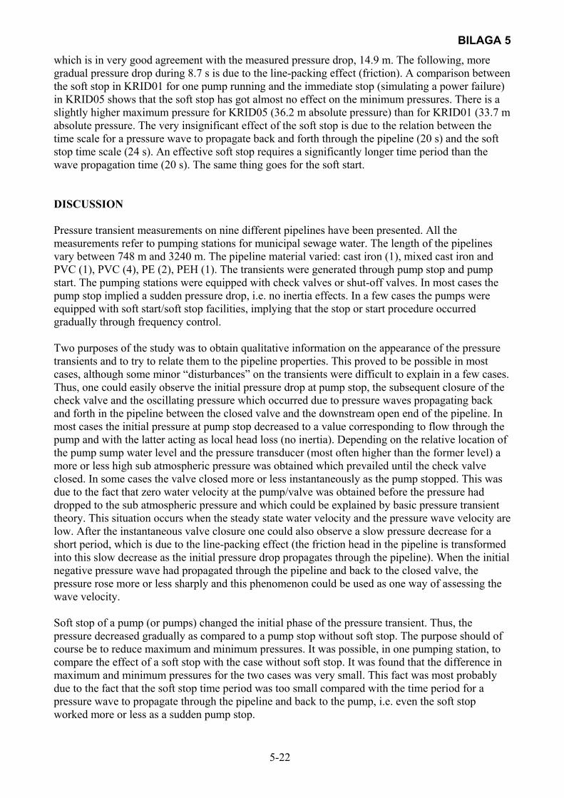
BILAGA 5

5-22

which is in very good agreement with the measured pressure drop, 14.9 m. The following, more gradual pressure drop during 8.7 s is due to the line-packing effect (friction). A comparison between the soft stop in KRID01 for one pump running and the immediate stop (simulating a power failure) in KRID05 shows that the soft stop has got almost no effect on the minimum pressures. There is a slightly higher maximum pressure for KRID05 (36.2 m absolute pressure) than for KRID01 (33.7 m absolute pressure. The very insignificant effect of the soft stop is due to the relation between the time scale for a pressure wave to propagate back and forth through the pipeline (20 s) and the soft stop time scale (24 s). An effective soft stop requires a significantly longer time period than the wave propagation time (20 s). The same thing goes for the soft start. DISCUSSION Pressure transient measurements on nine different pipelines have been presented. All the measurements refer to pumping stations for municipal sewage water. The length of the pipelines vary between 748 m and 3240 m. The pipeline material varied: cast iron (1), mixed cast iron and PVC (1), PVC (4), PE (2), PEH (1). The transients were generated through pump stop and pump start. The pumping stations were equipped with check valves or shut-off valves. In most cases the pump stop implied a sudden pressure drop, i.e. no inertia effects. In a few cases the pumps were equipped with soft start/soft stop facilities, implying that the stop or start procedure occurred gradually through frequency control. Two purposes of the study was to obtain qualitative information on the appearance of the pressure transients and to try to relate them to the pipeline properties. This proved to be possible in most cases, although some minor “disturbances” on the transients were difficult to explain in a few cases. Thus, one could easily observe the initial pressure drop at pump stop, the subsequent closure of the check valve and the oscillating pressure which occurred due to pressure waves propagating back and forth in the pipeline between the closed valve and the downstream open end of the pipeline. In most cases the initial pressure at pump stop decreased to a value corresponding to flow through the pump and with the latter acting as local head loss (no inertia). Depending on the relative location of the pump sump water level and the pressure transducer (most often higher than the former level) a more or less high sub atmospheric pressure was obtained which prevailed until the check valve closed. In some cases the valve closed more or less instantaneously as the pump stopped. This was due to the fact that zero water velocity at the pump/valve was obtained before the pressure had dropped to the sub atmospheric pressure and which could be explained by basic pressure transient theory. This situation occurs when the steady state water velocity and the pressure wave velocity are low. After the instantaneous valve closure one could also observe a slow pressure decrease for a short period, which is due to the line-packing effect (the friction head in the pipeline is transformed into this slow decrease as the initial pressure drop propagates through the pipeline). When the initial negative pressure wave had propagated through the pipeline and back to the closed valve, the pressure rose more or less sharply and this phenomenon could be used as one way of assessing the wave velocity. Soft stop of a pump (or pumps) changed the initial phase of the pressure transient. Thus, the pressure decreased gradually as compared to a pump stop without soft stop. The purpose should of course be to reduce maximum and minimum pressures. It was possible, in one pumping station, to compare the effect of a soft stop with the case without soft stop. It was found that the difference in maximum and minimum pressures for the two cases was very small. This fact was most probably due to the fact that the soft stop time period was too small compared with the time period for a pressure wave to propagate through the pipeline and back to the pump, i.e. even the soft stop worked more or less as a sudden pump stop.

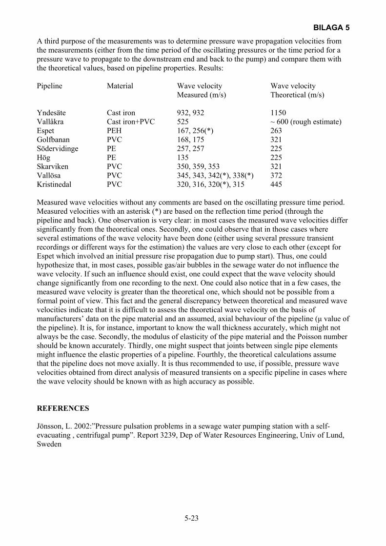
BILAGA 5

5-23

A third purpose of the measurements was to determine pressure wave propagation velocities from the measurements (either from the time period of the oscillating pressures or the time period for a pressure wave to propagate to the downstream end and back to the pump) and compare them with the theoretical values, based on pipeline properties. Results: Pipeline Material Wave velocity Wave velocity Measured (m/s) Theoretical (m/s) Yndesäte Cast iron 932, 932 1150 Vallåkra Cast iron+PVC 525 ~ 600 (rough estimate) Espet PEH 167, 256(*) 263 Golfbanan PVC 168, 175 321 Södervidinge PE 257, 257 225 Hög PE 135 225 Skarviken PVC 350, 359, 353 321 Vallösa PVC 345, 343, 342(*), 338(*) 372 Kristinedal PVC 320, 316, 320(*), 315 445 Measured wave velocities without any comments are based on the oscillating pressure time period. Measured velocities with an asterisk (*) are based on the reflection time period (through the pipeline and back). One observation is very clear: in most cases the measured wave velocities differ significantly from the theoretical ones. Secondly, one could observe that in those cases where several estimations of the wave velocity have been done (either using several pressure transient recordings or different ways for the estimation) the values are very close to each other (except for Espet which involved an initial pressure rise propagation due to pump start). Thus, one could hypothesize that, in most cases, possible gas/air bubbles in the sewage water do not influence the wave velocity. If such an influence should exist, one could expect that the wave velocity should change significantly from one recording to the next. One could also notice that in a few cases, the measured wave velocity is greater than the theoretical one, which should not be possible from a formal point of view. This fact and the general discrepancy between theoretical and measured wave velocities indicate that it is difficult to assess the theoretical wave velocity on the basis of manufacturers’ data on the pipe material and an assumed, axial behaviour of the pipeline (µ value of the pipeline). It is, for instance, important to know the wall thickness accurately, which might not always be the case. Secondly, the modulus of elasticity of the pipe material and the Poisson number should be known accurately. Thirdly, one might suspect that joints between single pipe elements might influence the elastic properties of a pipeline. Fourthly, the theoretical calculations assume that the pipeline does not move axially. It is thus recommended to use, if possible, pressure wave velocities obtained from direct analysis of measured transients on a specific pipeline in cases where the wave velocity should be known with as high accuracy as possible. REFERENCES Jönsson, L. 2002:”Pressure pulsation problems in a sewage water pumping station with a self-evacuating , centrifugal pump”. Report 3239, Dep of Water Resources Engineering, Univ of Lund, Sweden

BILAGA 5

5-24

Fig 1. Pump curve Yndesäte

Fig 2. Yndesäte. Stop of one pump

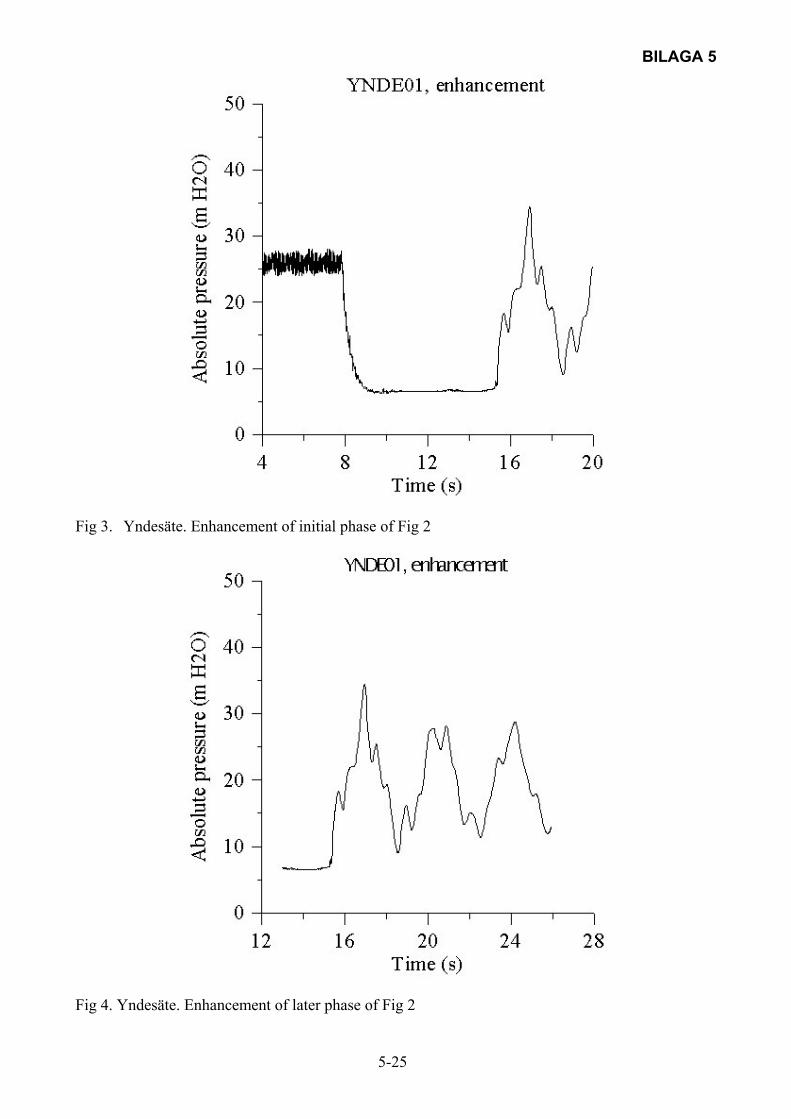
BILAGA 5

5-25

Fig 3. Yndesäte. Enhancement of initial phase of Fig 2

Fig 4. Yndesäte. Enhancement of later phase of Fig 2

BILAGA 5

5-26

Fig 5. Yndesäte. Stop of one pump

Fig 6. Yndesäte. Enhancement of the initial phase of Fig 5

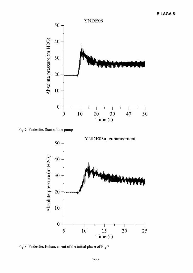
BILAGA 5

5-27

Fig 7. Yndesäte. Start of one pump

Fig 8. Yndesäte. Enhancement of the initial phase of Fig 7

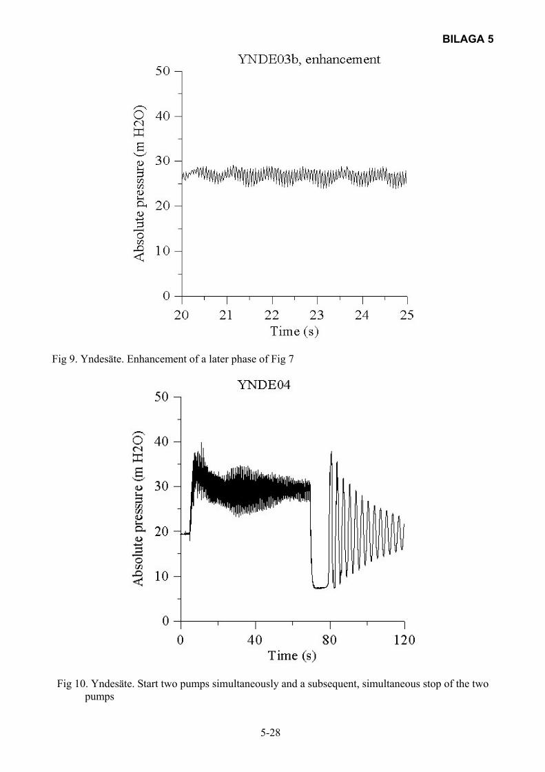
BILAGA 5

5-28

Fig 9. Yndesäte. Enhancement of a later phase of Fig 7

Fig 10. Yndesäte. Start two pumps simultaneously and a subsequent, simultaneous stop of the two

pumps

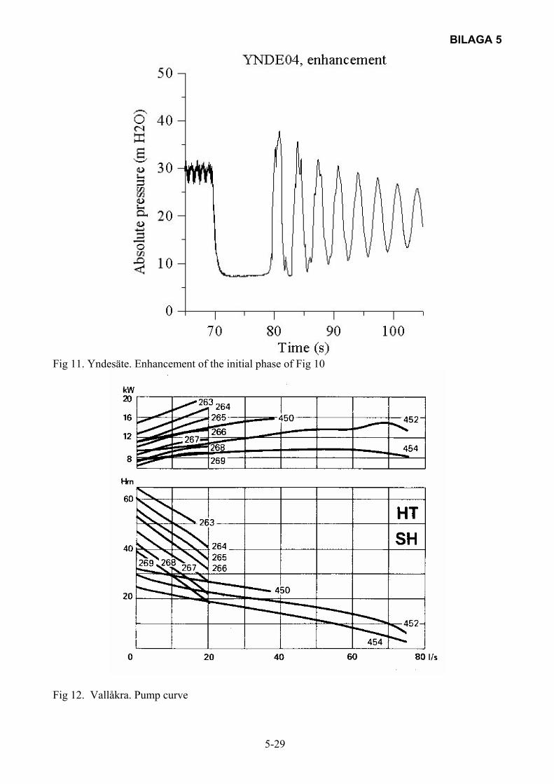
BILAGA 5

5-29

Fig 11. Yndesäte. Enhancement of the initial phase of Fig 10

Fig 12. Vallåkra. Pump curve

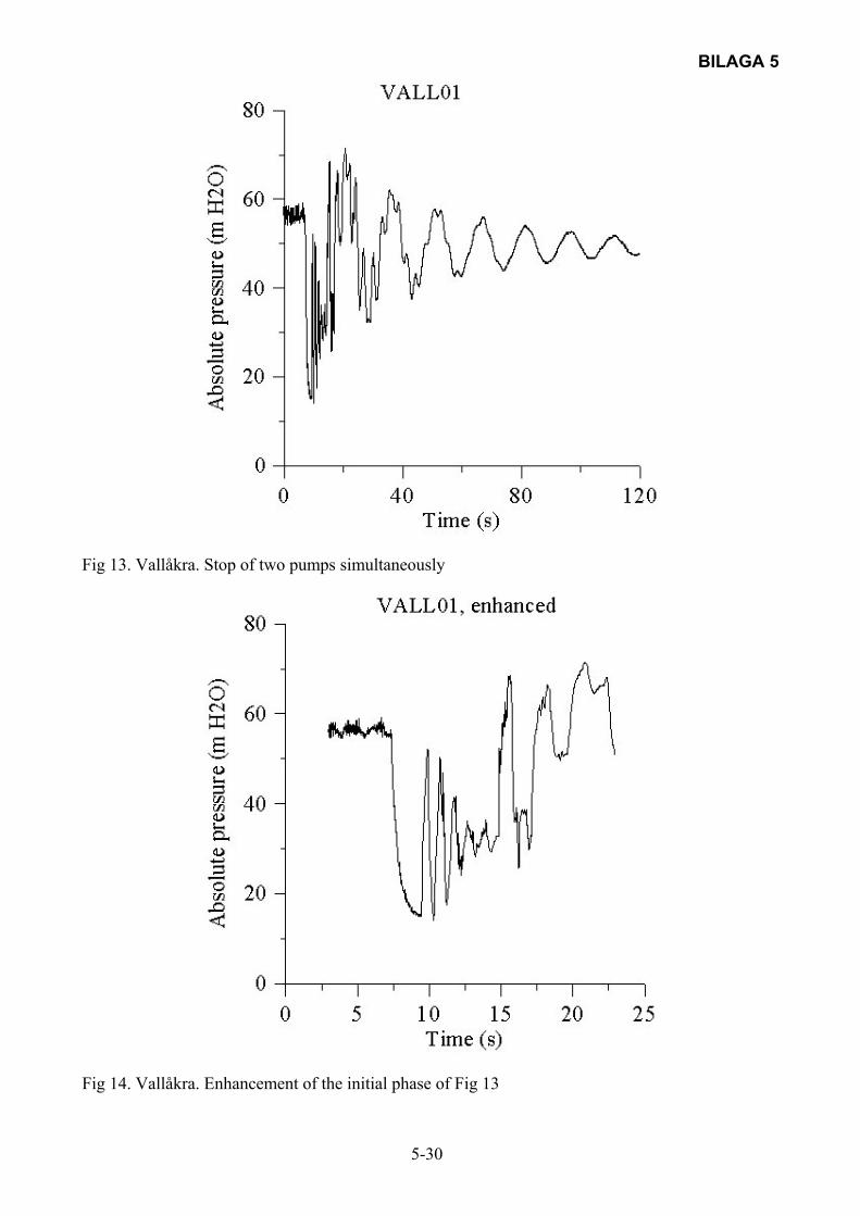
BILAGA 5

5-30

Fig 13. Vallåkra. Stop of two pumps simultaneously

Fig 14. Vallåkra. Enhancement of the initial phase of Fig 13

BILAGA 5

5-31

Fig 15. Vallåkra. Stop downstream pump first and then the upstream pump

Fig 16. Vallåkra. Start of upstream pump and subsequently the downstream pump

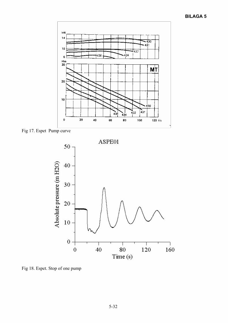
BILAGA 5

5-32

Fig 17. Espet Pump curve

Fig 18. Espet. Stop of one pump

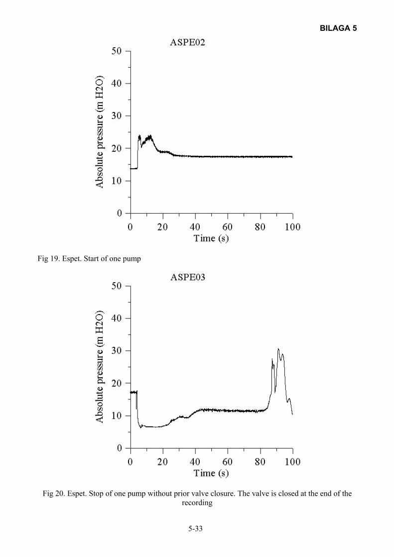
BILAGA 5

5-33

Fig 19. Espet. Start of one pump

Fig 20. Espet. Stop of one pump without prior valve closure. The valve is closed at the end of the recording

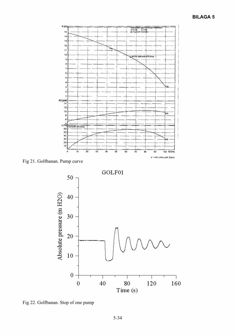
BILAGA 5

5-34

Fig 21. Golfbanan. Pump curve

Fig 22. Golfbanan. Stop of one pump

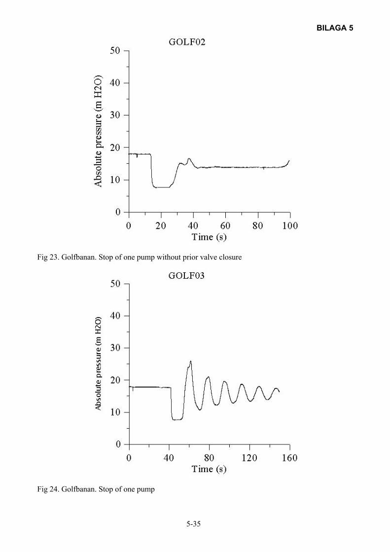
BILAGA 5

5-35

Fig 23. Golfbanan. Stop of one pump without prior valve closure

Fig 24. Golfbanan. Stop of one pump

BILAGA 5

5-36

Fig 25. Södervidinge. Pumping station

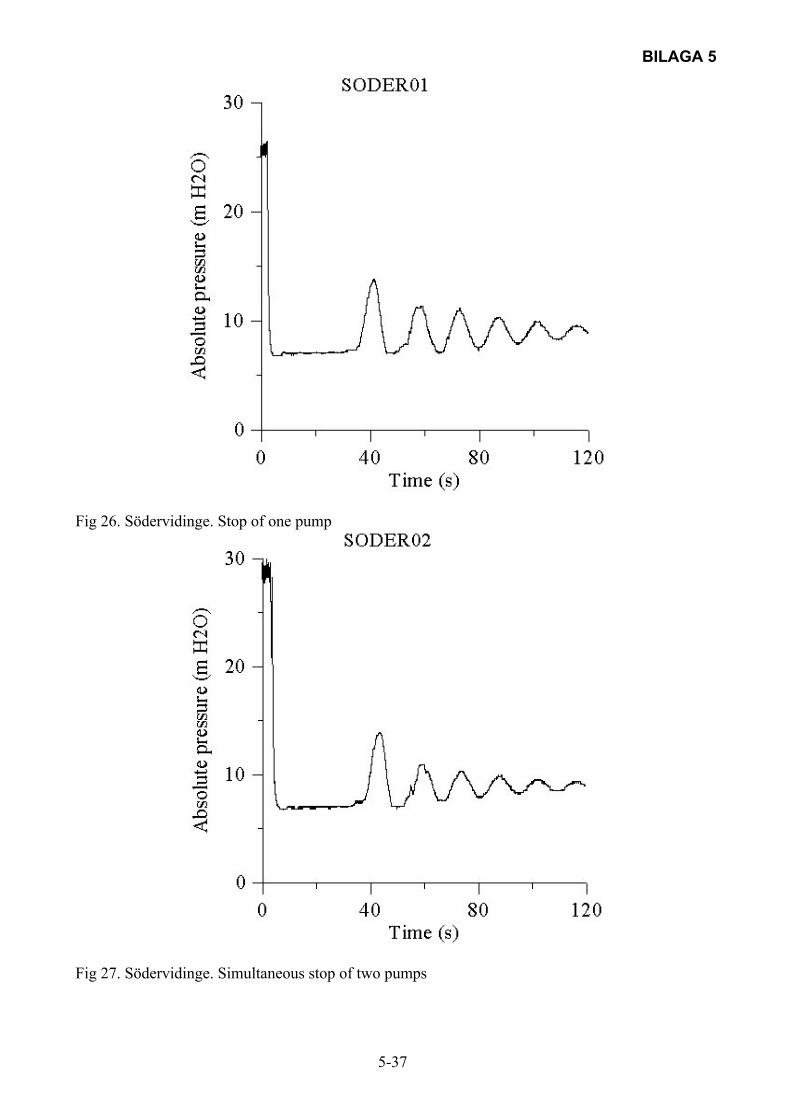
BILAGA 5

5-37

Fig 26. Södervidinge. Stop of one pump

Fig 27. Södervidinge. Simultaneous stop of two pumps

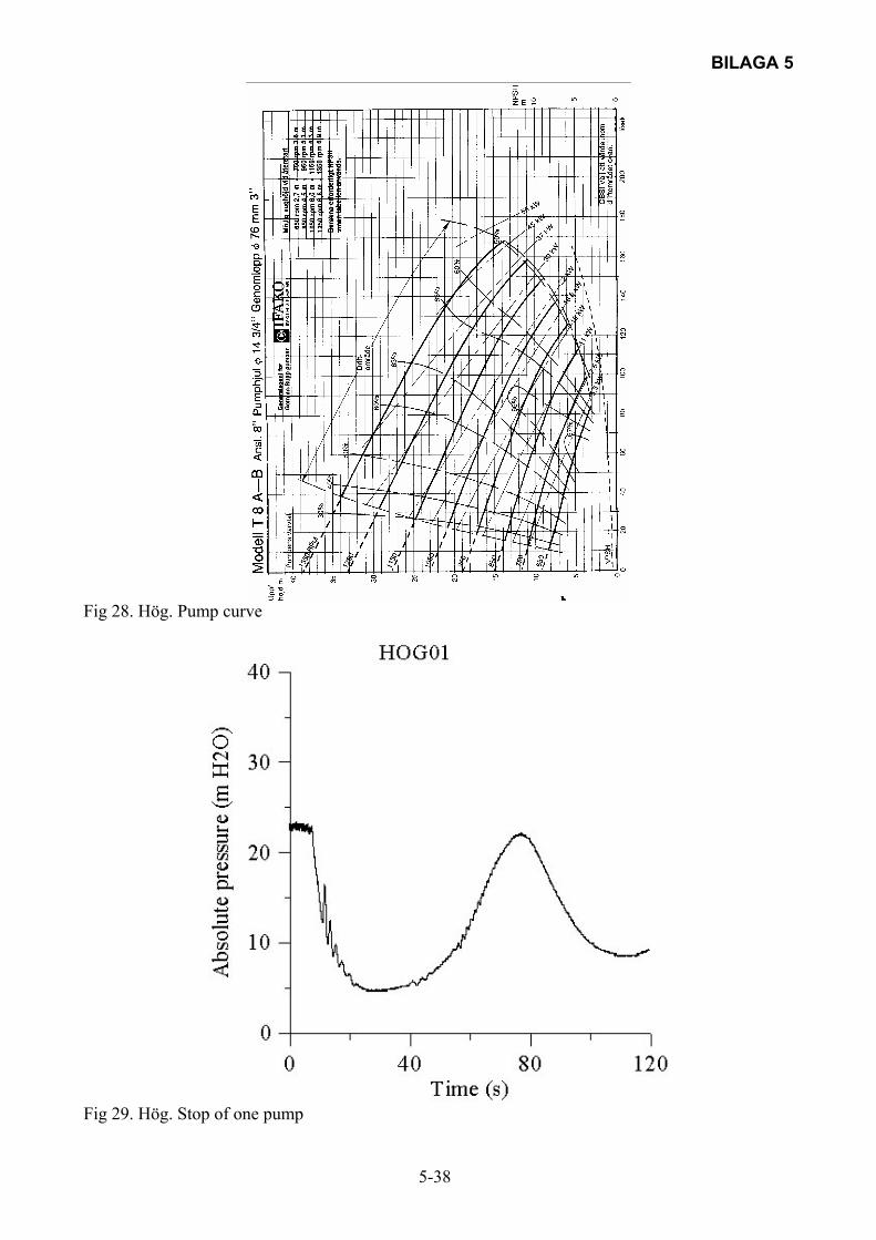
BILAGA 5

5-38

Fig 28. Hög. Pump curve

Fig 29. Hög. Stop of one pump

BILAGA 5

5-39

Fig 30. Hög. Enhancement of the initial phase of Fig 29

Fig 31. Hög. Stop of one pump

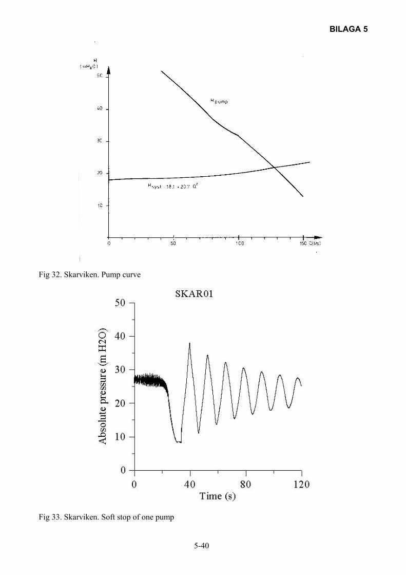
BILAGA 5

5-40

Fig 32. Skarviken. Pump curve

Fig 33. Skarviken. Soft stop of one pump

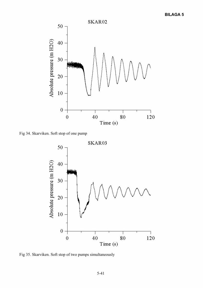
BILAGA 5

5-41

Fig 34. Skarviken. Soft stop of one pump

Fig 35. Skarviken. Soft stop of two pumps simultaneously

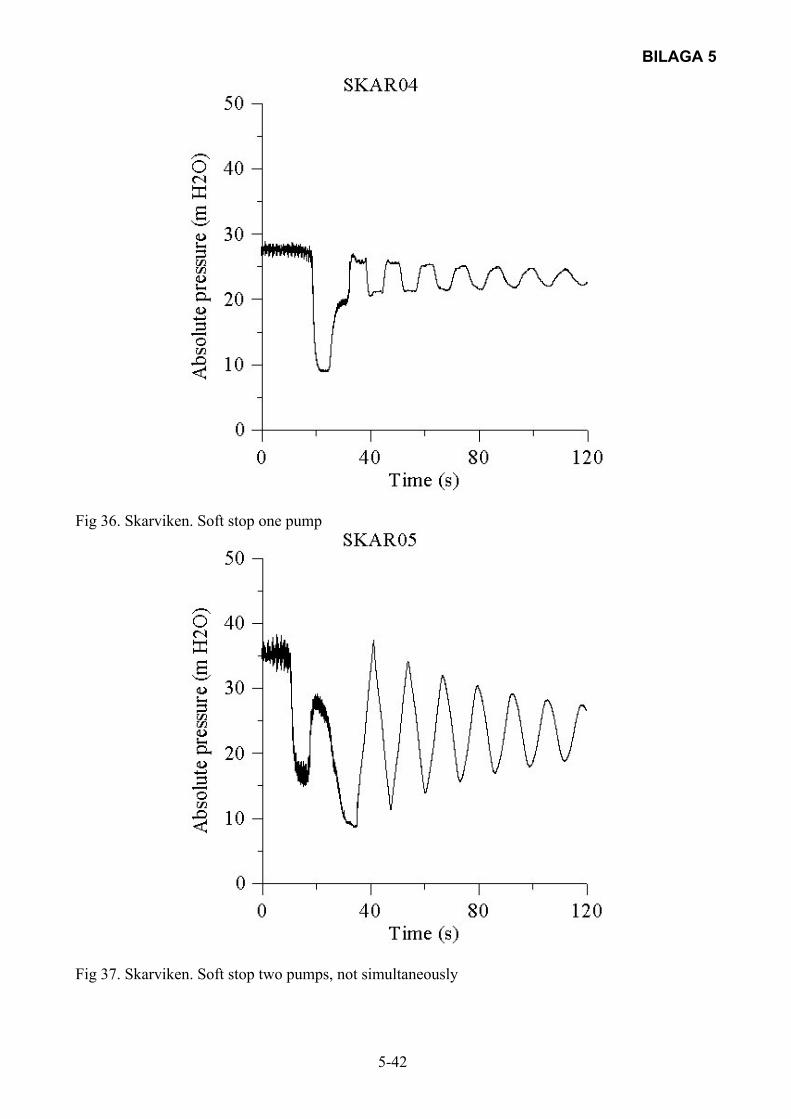
BILAGA 5

5-42

Fig 36. Skarviken. Soft stop one pump

Fig 37. Skarviken. Soft stop two pumps, not simultaneously

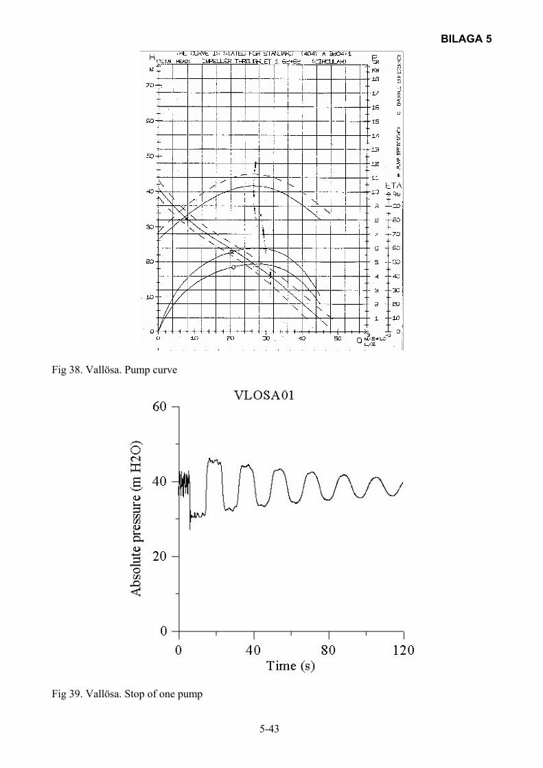
BILAGA 5

5-43

Fig 38. Vallösa. Pump curve

Fig 39. Vallösa. Stop of one pump

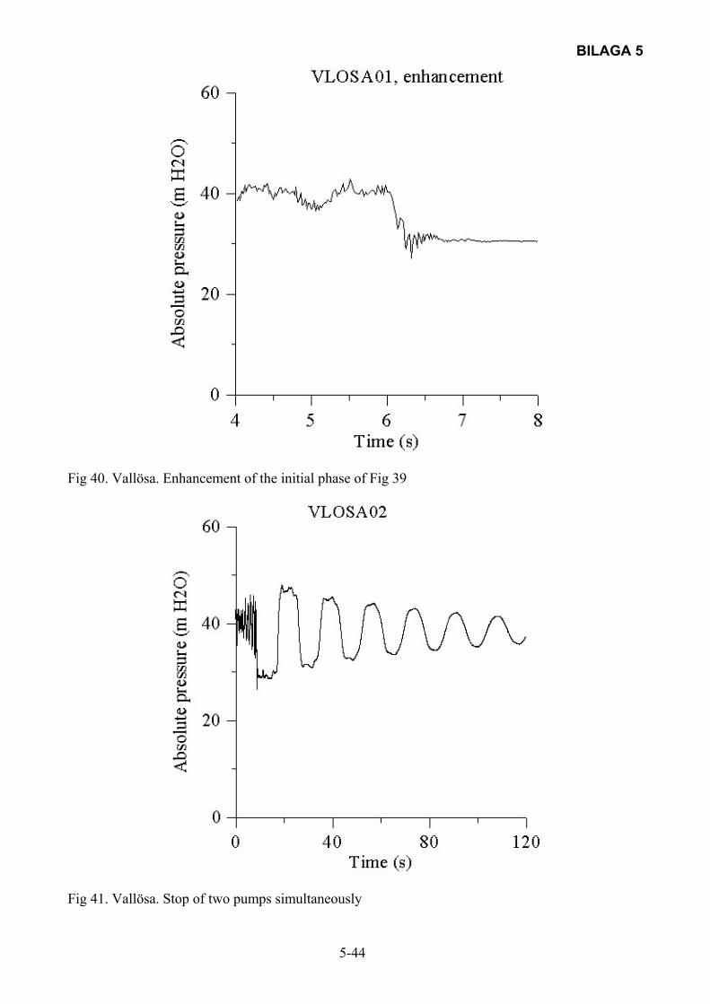
BILAGA 5

5-44

Fig 40. Vallösa. Enhancement of the initial phase of Fig 39

Fig 41. Vallösa. Stop of two pumps simultaneously

BILAGA 5

5-45

Fig 42. Vallösa. Enhancement of the initial phase of Fig 41

Fig 43. Vallösa. Stop of two pumps, not simultaneously

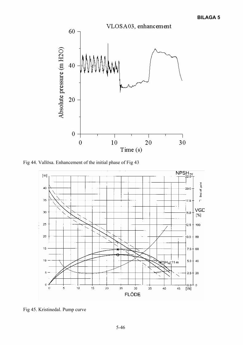
BILAGA 5

5-46

Fig 44. Vallösa. Enhancement of the initial phase of Fig 43

Fig 45. Kristinedal. Pump curve

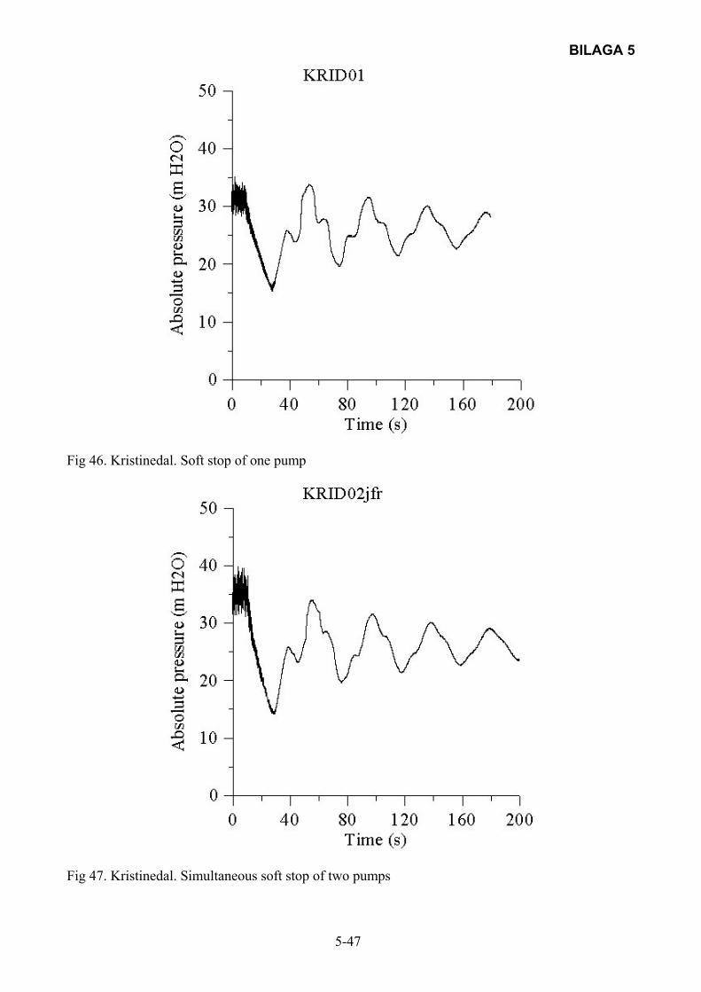
BILAGA 5

5-47

Fig 46. Kristinedal. Soft stop of one pump

Fig 47. Kristinedal. Simultaneous soft stop of two pumps

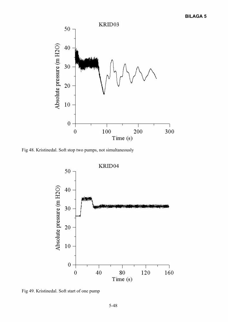
BILAGA 5

5-48

Fig 48. Kristinedal. Soft stop two pumps, not simultaneously

Fig 49. Kristinedal. Soft start of one pump

BILAGA 5

5-49

Fig 50. Kristinedal. Instantaneous (no soft stop) stop of one pump.

Box 47607 117 94 Stockholm Tfn 08-506 002 00 Fax 08-506 002 10 E-post svensktvatten@svensktvatten.se www.svensktvatten.se

Trycktransienter i rörsystem

för vattentransp

ort – p

rob

lem o

ch nytta