Embed Size (px)
Citation preview
Centro de Investigacion y de EstudiosAvanzados
del Instituto Politecnico Nacional
Unidad Zacatenco
Departamento de Computacion
Mapeo de Celda a Celda para Optimizacion Global
Multi-objetivo
Tesis que presenta
Carlos Ignacio Hernandez Castellanos
obtener el Grado de
Maestro en Ciencias
en Computacion
Director de la Tesis:
Dr. Oliver Schutze
Mexico, D.F Agosto 2013

ii
Centro de Investigacion y de EstudiosAvanzados
del Instituto Politecnico Nacional
Zacatenco Campus
Computer Science Department
Cell-to-Cell Mapping for Global Multi-Objective
Optimization
Submitted by
Carlos Ignacio Hernandez Castellanos
as fulfillment of the requirement for the degree of
Master in
Computer Science
Advisor:
Dr. Oliver Schutze
Mexico, D.F August 2013

iv
v
Resumen
De manera frecuente nos encontramos con el problema de optimizar varios obje-tivos de manera simultanea y tıpicamente estos objetivos estan en conflicto entre ellos.A este tipo de problemas se les conoce con el nombre de problemas de optimizacionmulti-objetivo (POM). En la mayorıa de los casos la solucion a estos problemas no esunica, si no un compromiso entre los objetivos.
En esta tesis, presentamos metodos orientados a conjuntos para resolver estosproblemas. En particular, nos enfocamos al problema de encontrar el conjunto desoluciones optimas, ası como el problema de encontrar el conjunto de soluciones aprox-imadas de un problema de optimizacion multi-objetivo. Este ultimo conjunto es deinteres para el tomador de decisiones, dado que le puede proporcionar soluciones adi-cionales a las optimas para la implementacion de su proyecto relacionado al POM.En este estudio, hacemos una primera adaptacion de las bien conocidas tecnicasde mapeo de celdas para el analisis global de sistemas dinamicos del problema encuestion. Dado el caracter global del enfoque, estos metodos son adecuados para lainvestigacion exhaustiva de problemas pequenos, incluyendo el computo del conjuntode soluciones aproximadas. Tambien mostramos que nuestra propuesta es competitivacon los algoritmos evolutivos para problemas de un numero bajo de dimensiones.
vi
Abstract
One is frequently faced with the problem of optimizing several objectives simul-taneously and typically these objectives are in conflict with each other. These kindof problems are known as multi-objective optimization problems (MOPs). Typically,the solution set of a given MOP does not consist of a single point as for single ob-jective optimization problems but forms a k − 1 dimensional entity where k is thenumber of objectives involved in the MOP.
In this thesis, we present set oriented methods for the treatment of these problems.In particular, we address the problem of computing the set of optimal solutions as wellas the set approximate solutions of a given MOP. The later set is of potential interestfor the decision maker since it might give him/her additional solutions to the optimalones for the realization of the project related to the MOP. In this study, we makea first attempt to adapt well-known cell mapping techniques for the global analysisof dynamical systems related to the problem at hand. Due to their global approach,these methods are well-suited for the thorough investigation of small problems, in-cluding the computation of the set of approximate solutions. We also show thatthe proposed approach is competitive to evolutionary strategies for low dimensionalproblems.

vii
Acknowledgment
First, I would like to thank the CONACyT for the scholarship given by them forthe pursuit of my master’s studies.
Also, I want to thank the CINVESTAV and specially to the computer science de-partment, to all my professors, to the secretaries and to my colleagues for all thatthey have thought me in the past two years.
Further, I would like to acknowledge my advisor Dr. Oliver Schutze for his sup-port and guidance through this project.
Finally, I would like to give an special acknowledgement to my family that haveall ways supported me.

viii
Contents
List of Figures xi
List of Tables xiv
List of Algorithms xv
1 Introduction 1
1.1 Motivation . . . . . . . . . . . . . . . . . . . . . . . . . . . . . . . . . 1
1.2 The Problem . . . . . . . . . . . . . . . . . . . . . . . . . . . . . . . 2
1.3 Objectives . . . . . . . . . . . . . . . . . . . . . . . . . . . . . . . . . 2
1.4 Contributions . . . . . . . . . . . . . . . . . . . . . . . . . . . . . . . 3
1.5 Organization of the thesis . . . . . . . . . . . . . . . . . . . . . . . . 4
2 Background and Related Work 5
2.1 Multi-objective Optimization . . . . . . . . . . . . . . . . . . . . . . 5
2.1.1 Formulation of the Problem . . . . . . . . . . . . . . . . . . . 6
2.1.2 Pareto Optimality . . . . . . . . . . . . . . . . . . . . . . . . 6
2.1.3 Optimality conditions . . . . . . . . . . . . . . . . . . . . . . 9
2.1.4 Descent directions . . . . . . . . . . . . . . . . . . . . . . . . . 10
2.2 Solving MOPs . . . . . . . . . . . . . . . . . . . . . . . . . . . . . . . 10
2.2.1 Scalarization methods . . . . . . . . . . . . . . . . . . . . . . 10
2.2.2 Descent direction methods . . . . . . . . . . . . . . . . . . . . 13
2.2.3 Stochastic methods . . . . . . . . . . . . . . . . . . . . . . . . 16
2.2.4 Performance Measures . . . . . . . . . . . . . . . . . . . . . . 17
2.3 Dynamical Systems . . . . . . . . . . . . . . . . . . . . . . . . . . . . 19
2.3.1 Formulation of the problem . . . . . . . . . . . . . . . . . . . 19
2.3.2 Fixed point . . . . . . . . . . . . . . . . . . . . . . . . . . . . 20
2.3.3 Periodic group . . . . . . . . . . . . . . . . . . . . . . . . . . . 20
2.3.4 Domain of attraction . . . . . . . . . . . . . . . . . . . . . . . 20
2.4 Global Analysis of Dynamical Systems . . . . . . . . . . . . . . . . . 20
2.4.1 Discretization of the space . . . . . . . . . . . . . . . . . . . . 20
2.4.2 Simple cell mapping . . . . . . . . . . . . . . . . . . . . . . . 21
2.4.3 Subdivision techniques . . . . . . . . . . . . . . . . . . . . . . 23
ix
x CONTENTS
3 SCM for MOO 273.1 Simple Cell Mapping . . . . . . . . . . . . . . . . . . . . . . . . . . . 27
3.1.1 Description of the SCM Method . . . . . . . . . . . . . . . . . 273.1.2 Center point method . . . . . . . . . . . . . . . . . . . . . . . 283.1.3 Analysis of SCM . . . . . . . . . . . . . . . . . . . . . . . . . 32
3.2 Adapting the SCM Method for MOPs . . . . . . . . . . . . . . . . . . 323.2.1 Dynamical system . . . . . . . . . . . . . . . . . . . . . . . . 333.2.2 Step size control . . . . . . . . . . . . . . . . . . . . . . . . . 333.2.3 Finding Pareto optimal solutions . . . . . . . . . . . . . . . . 34
3.3 Description the SCM method for MOPs . . . . . . . . . . . . . . . . 353.4 Numerical Results . . . . . . . . . . . . . . . . . . . . . . . . . . . . . 38
3.4.1 Problem 1 . . . . . . . . . . . . . . . . . . . . . . . . . . . . . 383.4.2 Problem 2 . . . . . . . . . . . . . . . . . . . . . . . . . . . . . 393.4.3 Problem 3 . . . . . . . . . . . . . . . . . . . . . . . . . . . . . 393.4.4 Problem 4 . . . . . . . . . . . . . . . . . . . . . . . . . . . . . 39
4 SCM for Approximate Solutions 494.1 Archiving Techniques . . . . . . . . . . . . . . . . . . . . . . . . . . . 504.2 Description of SCM for Approximate Solutions . . . . . . . . . . . . . 514.3 Numerical Results . . . . . . . . . . . . . . . . . . . . . . . . . . . . . 52
4.3.1 Problem 1 . . . . . . . . . . . . . . . . . . . . . . . . . . . . . 554.3.2 Problem 2 . . . . . . . . . . . . . . . . . . . . . . . . . . . . . 554.3.3 Problem 3 . . . . . . . . . . . . . . . . . . . . . . . . . . . . . 57
5 Analysis of Descent Direction Methods 615.1 The Problem . . . . . . . . . . . . . . . . . . . . . . . . . . . . . . . 615.2 Empirical Comparison of DDMs . . . . . . . . . . . . . . . . . . . . . 625.3 Comparison of DDMs by SCM . . . . . . . . . . . . . . . . . . . . . . 625.4 Numerical Results . . . . . . . . . . . . . . . . . . . . . . . . . . . . . 64
5.4.1 Problem 1 . . . . . . . . . . . . . . . . . . . . . . . . . . . . . 645.4.2 Problem 2 . . . . . . . . . . . . . . . . . . . . . . . . . . . . . 645.4.3 Problem 3 . . . . . . . . . . . . . . . . . . . . . . . . . . . . . 64
6 Refine and Recover 716.1 Refine . . . . . . . . . . . . . . . . . . . . . . . . . . . . . . . . . . . 71
6.1.1 Refine in Cell . . . . . . . . . . . . . . . . . . . . . . . . . . . 716.1.2 SCM-Refine . . . . . . . . . . . . . . . . . . . . . . . . . . . . 726.1.3 SCM with subdivision techniques . . . . . . . . . . . . . . . . 736.1.4 Comparison of the methods . . . . . . . . . . . . . . . . . . . 73
6.2 Recover . . . . . . . . . . . . . . . . . . . . . . . . . . . . . . . . . . 746.2.1 Moving Boxes . . . . . . . . . . . . . . . . . . . . . . . . . . . 746.2.2 Continuation . . . . . . . . . . . . . . . . . . . . . . . . . . . 766.2.3 Comparison of the methods . . . . . . . . . . . . . . . . . . . 76

CONTENTS xi
7 Conclusions and Future Work 797.1 Conclusions . . . . . . . . . . . . . . . . . . . . . . . . . . . . . . . . 797.2 Future Work . . . . . . . . . . . . . . . . . . . . . . . . . . . . . . . . 80
A Appendix A: Test Functions 81
Bibliography 89

xii CONTENTS
List of Figures
2.1 Pareto Dominance . . . . . . . . . . . . . . . . . . . . . . . . . . . . 72.2 Pareto set and Pareto front . . . . . . . . . . . . . . . . . . . . . . . 82.3 Approximate solutions . . . . . . . . . . . . . . . . . . . . . . . . . . 92.4 Curve of dominated points . . . . . . . . . . . . . . . . . . . . . . . . 132.5 Group Motion . . . . . . . . . . . . . . . . . . . . . . . . . . . . . . . 222.6 Simple Cell Mapping . . . . . . . . . . . . . . . . . . . . . . . . . . . 232.7 Subdivision Techniques . . . . . . . . . . . . . . . . . . . . . . . . . . 25
3.1 Neighborhood of a point . . . . . . . . . . . . . . . . . . . . . . . . . 283.2 Periodic motion and global properties of a cell . . . . . . . . . . . . . 293.3 Cell Mapping . . . . . . . . . . . . . . . . . . . . . . . . . . . . . . . 313.4 Step size control for SCM . . . . . . . . . . . . . . . . . . . . . . . . 343.5 Iterations of SCM . . . . . . . . . . . . . . . . . . . . . . . . . . . . . 363.6 SCM on MOP (A.1) on cell space . . . . . . . . . . . . . . . . . . . . 383.7 Effect of grid size on SCM . . . . . . . . . . . . . . . . . . . . . . . . 413.8 SCM for three Academic models on cell space . . . . . . . . . . . . . 423.9 Numerical results for MOP (A.1 in page 81) . . . . . . . . . . . . . . 433.10 Numerical results for MOP (A.2 in page 82) . . . . . . . . . . . . . . 443.11 Numerical results for MOP (A.3 in page 83) with n = 3 . . . . . . . . 453.12 Numerical results for MOP (A.3 in page 83) with n = 5 . . . . . . . . 463.13 Numerical results for PID problem (A.6) . . . . . . . . . . . . . . . . 47
4.1 Iterations of SCM for PQε . . . . . . . . . . . . . . . . . . . . . . . . 534.2 Impact of epsilon values . . . . . . . . . . . . . . . . . . . . . . . . . 544.3 SCM on MOP (A.1) for PQ,ε on cell space . . . . . . . . . . . . . . . 554.4 Numerical results for MOP (A.1 in page 81) for PQ,ε . . . . . . . . . . 564.5 Numerical results for MOP (A.2 in page 82) for PQ,ε . . . . . . . . . . 584.6 Numerical results for MOP (A.3 in page 83) for PQ,ε . . . . . . . . . . 594.7 Hypothetical decision making problem for MOP (A.2) . . . . . . . . . 60
5.1 Empirical Comparison of descent direction methods . . . . . . . . . . 635.2 SCM on MOP (A.1) in cell space with different descent direction meth-
ods. . . . . . . . . . . . . . . . . . . . . . . . . . . . . . . . . . . . . 655.3 Comparison of Domain of Attraction for MOP (A.1) . . . . . . . . . 66
xiii
xiv LIST OF FIGURES
5.4 SCM on MOP (A.4) in cell space with different descent direction meth-ods. . . . . . . . . . . . . . . . . . . . . . . . . . . . . . . . . . . . . 67
5.5 Comparison of Domain of Attraction for MOP (A.4) . . . . . . . . . 685.6 SCM on MOP (A.5) in cell space with different descent direction meth-
ods. . . . . . . . . . . . . . . . . . . . . . . . . . . . . . . . . . . . . 695.7 Comparison of Domain of Attraction for MOP (A.5) . . . . . . . . . 70
6.1 Comparison of refinement methods . . . . . . . . . . . . . . . . . . . 756.2 Comparison of recover methods . . . . . . . . . . . . . . . . . . . . . 77
A.1 Pareto set and Pareto front of MOP (A.1). . . . . . . . . . . . . . . . 81A.2 Pareto set and Pareto front of MOP (A.2). . . . . . . . . . . . . . . . 82A.3 Pareto set and Pareto front of MOP (A.3). . . . . . . . . . . . . . . . 83A.4 Pareto set and Pareto front of MOP (A.4). . . . . . . . . . . . . . . . 84A.5 Pareto set and Pareto front of MOP (A.5). . . . . . . . . . . . . . . . 85A.6 Pareto set and Pareto front of MOP (A.6). . . . . . . . . . . . . . . . 87
List of Tables
3.1 ∆p values for the distances of the candidate solution set to PQ,ε . . . 403.2 ∆p values for the distances of the images of the candidate sets to F (PQ,ε). 40
4.1 ∆p values for the distances of the candidate solution set to PQ,ε . . . 574.2 ∆p values for the distances of the images of the candidate sets to F (PQ,ε). 57
5.1 ∆p values for the distances of the candidate solution set to PQ,ε andF (PQ,ε) for MOP (A.1). . . . . . . . . . . . . . . . . . . . . . . . . . 62
6.1 ∆p values for the distances of the candidate solution set to PQ,ε andF (PQ,ε) for refinement methods . . . . . . . . . . . . . . . . . . . . . 74
6.2 ∆p values for the distances of the candidate solution set to PQ,ε andF (PQ,ε) for refinement methods . . . . . . . . . . . . . . . . . . . . . 77
xv

xvi LIST OF TABLES

List of Algorithms
1 PQ,ε-NSGA-II. . . . . . . . . . . . . . . . . . . . . . . . . . . . . . . . 172 Simple Cell Mapping Algorithm. . . . . . . . . . . . . . . . . . . . . . 303 Cell integer to cell coordinates . . . . . . . . . . . . . . . . . . . . . . 314 Cell coordinates to cell number. . . . . . . . . . . . . . . . . . . . . . 315 Simple Cell Mapping for MOPs. . . . . . . . . . . . . . . . . . . . . . 376 ArchiveUpdateTight2 . . . . . . . . . . . . . . . . . . . . . . . . . . . 517 Post-processing to get PQ,ε . . . . . . . . . . . . . . . . . . . . . . . . 528 Refine in Cell (rinc) . . . . . . . . . . . . . . . . . . . . . . . . . . . . 729 SCM-Refine . . . . . . . . . . . . . . . . . . . . . . . . . . . . . . . . 7310 Moving Boxes . . . . . . . . . . . . . . . . . . . . . . . . . . . . . . . 7611 SCM Continuation . . . . . . . . . . . . . . . . . . . . . . . . . . . . 76
xvii

xviii LIST OF ALGORITHMS
Chapter 1
Introduction
One is frequently faced with the problem of optimizing several objectives simultane-ously and typically these objectives are in conflict with each other. Such objectivescan be, for instance, the quality and the cost of a product. One would like to make aproduct, which has the highest quality, but at the same time the lowest cost. One cansee that, since the objectives are in conflict in this example, there is not one singlesolution, but rather a set of them, which in this case represents the trade-off betweenquality and cost. Thus, in applications one is confronted with the problem of findingthe best trade-off solutions for the given problems.
1.1 Motivation
So far, many numerical methods for the treatment of a given Multi-objective Op-timization Problem (MOP) have been proposed. There exist, for instance, manyscalarization methods that transform the MOP into a scalar optimization problem(SOP). By choosing a clever sequence of SOPs a finite size approximation of theentire Pareto set can be obtained in certain cases [1, 2, 3, 4]. Since the solutionset (the so-called Pareto set) forms under some mild regularity conditions locally a(k−1)-manifold, where k is the number of objectives involved in the MOP, specializedcontinuation methods, which perform a search along the Pareto set are very efficientif one solution is at hand [5, 6, 7, 8] and if the Pareto set is connected.
Another approach to approximate the Pareto set is to use set oriented methodssuch as subdivision techniques [9, 10, 11] or stochastic search methods [12, 13, 14].The advantage of such set based methods is that they generate an approximation ofthe (global) Pareto set in one single run of the algorithm. Further, they are applicableto a large range of optimization problems and are characterized by a great amountof robustness. Hence, these methods are interesting alternatives against ‘classical’mathematical programming techniques in particular for the thorough investigationof low or moderate dimensional MOPs. The method that is used in this study fallsinto the last category: Cell mapping techniques as proposed in [15] are coupled withdynamical systems derived from multi-objective descent directions that allow for the
1
2 CHAPTER 1. INTRODUCTION
computation of a suitable finite size approximation of the set of interest.
1.2 The Problem
The set of approximate solutions forms a n-dimensional object, where n is the numberof parameters. For this reason it might be useful to have the global view of MOPs tosee its behavior and then to compute the set of interest.
Some numerical schemes are proposed in [2, 16, 17, 18] to solve unconstrainedMOPs. The general idea is starting from an initial solution to steer the search processin a desired direction given in objective space. It is important to mention that forthese schemes the proposed process can be formulated as an initial value problem(IVP).
From that idea, if an IVP formulation is used to solve MOPs then we could makea match between Pareto optimal solutions and an attractor of this dynamical system.We would also be able to obtain the basin of attraction of every point of the Paretoset. However, to obtain the global view just by using this, we would have to followthe IVP for all points in parameter space, which is not possible in practice.
To solve this problem, let us point out that, since the representation of the numbersin a computer is finite, a number represents not only the number represented by itsdigits, but also an infinite neighborhood of numbers given by the precision of themachine. This does not allow to assume variables to be continuous, due to roundingerrors and for this reason it is possible to consider the space as small hypercubeswhose size is given by the machine precision.
The cell mapping approach [15] proposes to increase this discretization by dividingthe state space in bigger hypercubes called cells. The evolution of the dynamicalsystem is then reduced to a new function, which is defined not in Rn, but on the cellspace. In this case we restrict ourselves to functions that are strictly deterministicallydefined. For this case, we have the so-called simple cell mapping method.
The simple cell mapping method gives us a useful tool to obtain the attractors andbasins of attractions of a dynamical system. Thus, to extend this idea to the contextof multi-objective optimization, in order to obtain the set of approximate solutions isan important contribution.
1.3 Objectives
General Objective
To design set oriented methods for the numerical treatment of multi-objective opti-mization problems with a special attention to the set of approximate solutions.
1.4. CONTRIBUTIONS 3
Particular Objectives
1. To develop a simple cell mapping method for the computation of optimal solu-tions of a given MOP.
2. To develop a simple cell mapping method for the computation of the set ofapproximate solutions of a given MOP.
3. To hybridize simple cell mapping with subdivision techniques.
4. To study the domains of attraction for each descent direction method.
1.4 Contributions
• Set oriented algorithms for global multi-objective optimization
– Simple cell mapping for multi-objective optimization
– Simple cell mapping for the set of approximate solutions
• Comparison between descent direction methods by means of simple cell mapping
• Collaboration with the University of California at Merced
• Contribution at EVOLVE 2013 international conference: C. Hernandez, O.Schutze, J. Q. Sun. Computing the Set of Approximate Solutions of a Multi-Objective Optimization Problem by Means of Cell Mapping Techniques (pub-lished)
• Contribution at EVOLVE 2013 international conference: Y. Narajani, C. Hernandez,F. R. Xiong, O. Schutze, J. Q. Sun. A Hybrid Algorithm for the simple cellmapping Method in Multi-objective Optimization (published)
• Contribution at ASME 2013 international conference: Y. Sardahi, Y. Nara-jani, W. Liang, J. Q. Sun, C. Hernandez, O. Schutze. Multi-objective OptimalControl Design with the simple cell mapping Method (accepted)
• Contribution at CSTAM 2013 international conference: Y. Sardahi, Y. Nara-jani, W. Liang, F. R. Xiong, Z. C. Qin, Y. X., C. H., O. Schutze, J. Q. Sun.Multi-objective Optimal Design of Feedback Controls for Dynamical SystemsTime Delay (submitted)
• Contribution at International Journal of Dynamics and Control: C. Hernandez,Y. Narajani, Y. Sardahi, W. Liang, O. Schutze. simple cell mapping Methodfor Multiobjective Optimal PID Control Design (published)
4 CHAPTER 1. INTRODUCTION
1.5 Organization of the thesis
This thesis consists of seven chapters, including this introductory chapter. The re-mainder of this document is organized as follows:
Chapter 2 presents the basic concepts of multi-objective optimization and dynam-ical systems that are fundamental for understanding the current work. Further, wereview some of the methods for solving a multi-objective optimization problem alongwith some methods for global analysis of dynamical systems.
Chapter 3 is devoted to present the simple cell mapping Method in the context ofmulti-objective optimization. In this chapter, we discuss the key elements to adaptthis method and further on present numerical results on some academic models.
Chapter 4 describes the simple cell mapping for the set of approximate solutions.In this chapter, we present the elements that are incorporated to the method tocompute this set and we also present numerical results on academic models.
Chapter 5 provides a comparison between some of the different descent directionsin the literature. This is of particular interest to evolutionary algorithms, since a biasmay exist on this methods.
Chapter 6 includes a hybridization of the simple cell mapping with other tech-niques to help to refine its results and to recover solutions that may been lost whileperforming the search.
Finally, chapter 7 contains the conclusions and some possible future ideas to bedeveloped from this work.

Chapter 2
Background and Related Work
In this chapter, we look into the basic concepts that are needed for the understandingof this thesis work. We review the basic concepts of multi-objective optimization(Section 2.1) and dynamical systems (Section 2.3), which are the main topics relatedto this work. Further, we review some of the methods for solving a multi-objectiveoptimization problem (Section 2.2) and also methods which provide a global analysisof dynamical systems (Section 2.4).
2.1 Multi-objective Optimization
There is always the wish for getting things better, cheaper, quicker, etc. which isinherent in human nature. Optimization is the field that deals with this problem.Sometimes only one objective is selected to be optimized, this leads to what is knownas a single objective optimization problem (SOP). However, in many cases we havemore than one objective to be optimized and we need to consider them at the sametime. This leads to the so-called multi-objective optimization problems (MOPs).
In the first case, we can use our intuition to define what is better in terms of ourobjective. If we are in the context of minimization, we know that the lower the valueof the objective function, the better it is for our problem and we also know, that weare looking for “the solution”, i.e. we expect to find that one solution is better thanall the others.
In the second case, the problem gets more complicated because the definition ofwhat is “better” is not as easy to define as it was in the previous case. This leadsto another problem, since now we do not have “the solution” i.e, a unique one, butrather a set of solutions that are incomparable to each other.
In this section, we first define the multi-objective optimization problems (Section2.1.1), then we define optimality for MOPs along with our sets of interest (Section2.1.2). Next, we present the necessary optimality condition for MOPs (Section 2.1.3)and finally we introduce the concept of descent directions, which helps us to identifydirections toward optimal solutions can be found (Section 2.1.4).
5
6 CHAPTER 2. BACKGROUND AND RELATED WORK
2.1.1 Formulation of the Problem
The multi-objective optimization problem can be defined in its general form as
minx∈Rn{F (x)},
s.t.
gi(x) ≤ 0, i = 1, . . . , I,
hj(x) = 0, j = 1, . . . , J,
(2.1)
let Q ⊂ Rn be the feasible region defined by
Q = {x ∈ Rn|g(x) ≤ 0 + h(x) = 0}, (2.2)
where F : Q→ Rk is a vector consisting of the objective functions
fi : Q→ R, i = 1, . . . , k, (2.3)
x ∈ Q is known as a parameters vector, gi : Rn → R, i = 1, . . . , I is an inequalityconstraint and hi : Rn → R, j = 1, . . . , J is an equality constraint.
In case there are no constraints the MOP is known as unconstrained. We can alsosee that in case k = 1 the problem is a single-objective optimization problem (SOP). Itis important to notice that we could also state the MOP as a maximization problem,however, any maximization problem can be stated as a minimization problem, bymultiplying the objective function vector by −1. For the remainder of this documentwe will use the term MOP for problems where the feasible region is only defined bybox constraints QB
QB = {x|lbi ≤ xi ≤ ubi}, (2.4)
where lbi is the lower bound and ubi is the upper bound for xi, i = 1, . . . , n. Wewill also use the MOP as a minimization problem, which comes out without loss ofgenerality.
2.1.2 Pareto Optimality
Now, we need to define what is an optimal solution in the context of multi-objectiveoptimization. For the case k = 1 and given feasible points a, b ∈ Q with theirobjective values F (a), F (b) ∈ Rk, we would be able to say, that the one with thesmallest objective value is better by doing a comparison of the values. However, forthe case k > 1, it is not longer as simple as it was in the previous case, since doing thecomparison might end up with a solution being better according to one objective butworse according to another one. To overcome this problem, we introduce the conceptof Pareto dominance [19].
Definition 1 (Pareto Dominance) 1. Let v, w ∈ Rk. Then the vector v is lessthan w (denoted by v <p w), if vi < wi for all i ∈ 1, . . . , k. The relation ≤p isdefined analogously.
2.1. MULTI-OBJECTIVE OPTIMIZATION 7
P1
P2
P3
P4
P5
f1
f2
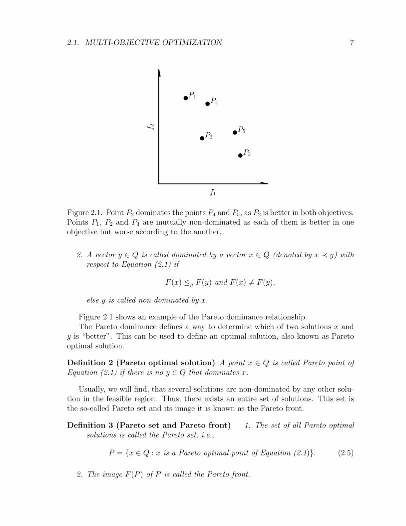
Figure 2.1: Point P2 dominates the points P4 and P5, as P2 is better in both objectives.Points P1, P2 and P3 are mutually non-dominated as each of them is better in oneobjective but worse according to the another.
2. A vector y ∈ Q is called dominated by a vector x ∈ Q (denoted by x ≺ y) withrespect to Equation (2.1) if
F (x) ≤p F (y) and F (x) 6= F (y),
else y is called non-dominated by x.
Figure 2.1 shows an example of the Pareto dominance relationship.The Pareto dominance defines a way to determine which of two solutions x and
y is “better”. This can be used to define an optimal solution, also known as Paretooptimal solution.
Definition 2 (Pareto optimal solution) A point x ∈ Q is called Pareto point ofEquation (2.1) if there is no y ∈ Q that dominates x.
Usually, we will find, that several solutions are non-dominated by any other solu-tion in the feasible region. Thus, there exists an entire set of solutions. This set isthe so-called Pareto set and its image it is known as the Pareto front.
Definition 3 (Pareto set and Pareto front) 1. The set of all Pareto optimalsolutions is called the Pareto set, i.e.,
P = {x ∈ Q : x is a Pareto optimal point of Equation (2.1)}. (2.5)
2. The image F (P ) of P is called the Pareto front.
8 CHAPTER 2. BACKGROUND AND RELATED WORK
−1 −0.5 0 0.5 1−1
−0.5
0
0.5
1
x1
x2
0 5 10 15 20
0
2
4
6
8
10
f1f2
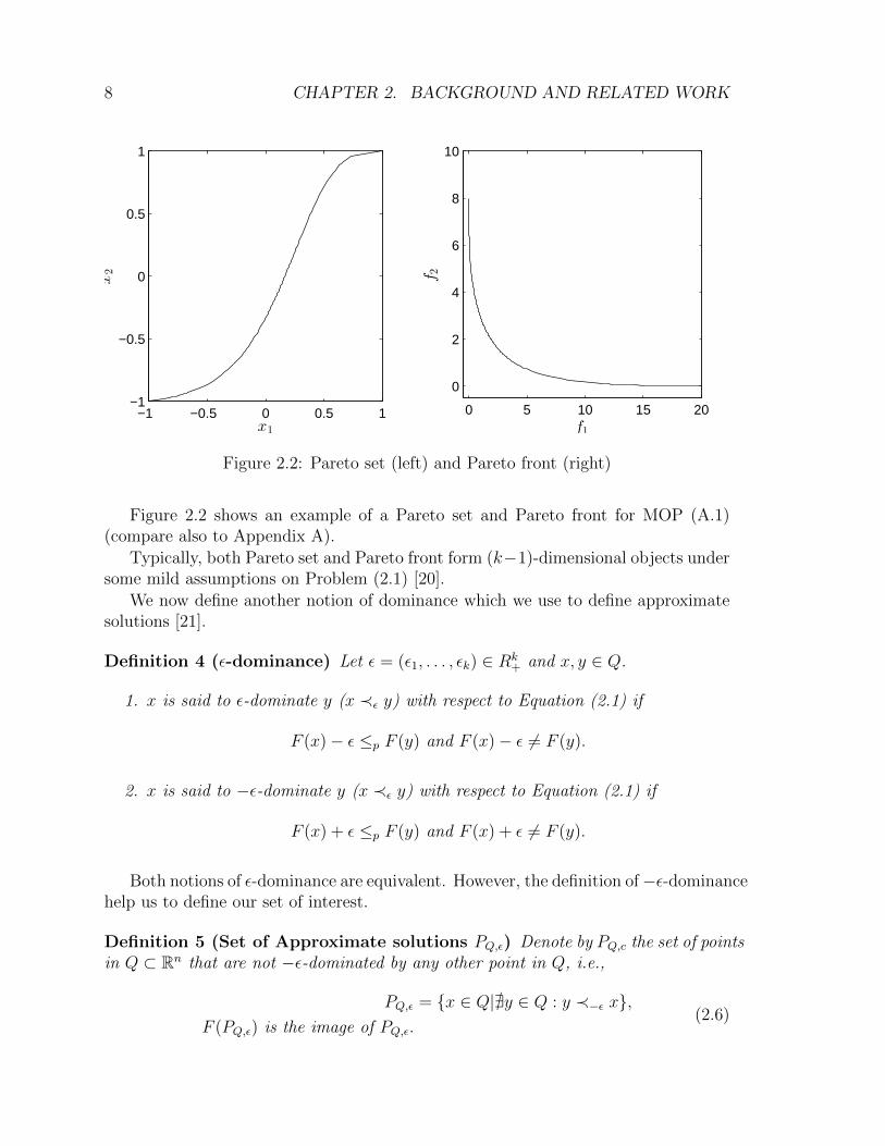
Figure 2.2: Pareto set (left) and Pareto front (right)
Figure 2.2 shows an example of a Pareto set and Pareto front for MOP (A.1)(compare also to Appendix A).
Typically, both Pareto set and Pareto front form (k−1)-dimensional objects undersome mild assumptions on Problem (2.1) [20].
We now define another notion of dominance which we use to define approximatesolutions [21].
Definition 4 (ε-dominance) Let ε = (ε1, . . . , εk) ∈ Rk+ and x, y ∈ Q.
1. x is said to ε-dominate y (x ≺ε y) with respect to Equation (2.1) if
F (x)− ε ≤p F (y) and F (x)− ε 6= F (y).
2. x is said to −ε-dominate y (x ≺ε y) with respect to Equation (2.1) if
F (x) + ε ≤p F (y) and F (x) + ε 6= F (y).
Both notions of ε-dominance are equivalent. However, the definition of−ε-dominancehelp us to define our set of interest.
Definition 5 (Set of Approximate solutions PQ,ε) Denote by PQ,c the set of pointsin Q ⊂ Rn that are not −ε-dominated by any other point in Q, i.e.,
PQ,ε = {x ∈ Q|@y ∈ Q : y ≺−ε x},F (PQ,ε) is the image of PQ,ε.
(2.6)
2.1. MULTI-OBJECTIVE OPTIMIZATION 9
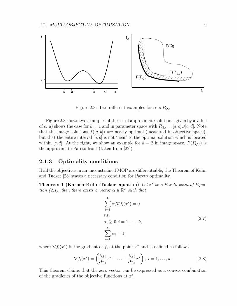
Figure 2.3: Two different examples for sets PQ,ε
Figure 2.3 shows two examples of the set of approximate solutions, given by a valueof ε. a) shows the case for k = 1 and in parameter space with PQ,ε = [a, b]∪[c, d]. Notethat the image solutions f([a, b]) are nearly optimal (measured in objective space),but that the entire interval [a, b] is not ‘near’ to the optimal solution which is locatedwithin [c, d]. At the right, we show an example for k = 2 in image space, F (PQ,ε) isthe approximate Pareto front (taken from [22]).
2.1.3 Optimality conditions
If all the objectives in an unconstrained MOP are differentiable, the Theorem of Kuhnand Tucker [23] states a necessary condition for Pareto optimality.
Theorem 1 (Karush-Kuhn-Tucker equation) Let x∗ be a Pareto point of Equa-tion (2.1), then there exists a vector α ∈ Rk such that
k∑i=1
αi∇fi(x∗) = 0
s.t.
αi ≥ 0, i = 1, . . . , k,
k∑i=1
αi = 1,
(2.7)
where ∇fi(x∗) is the gradient of fi at the point x∗ and is defined as follows
∇fi(x∗) =
(∂fi∂x1
x∗ + . . .+∂fi∂xn
x∗), i = 1, . . . , k. (2.8)
This theorem claims that the zero vector can be expressed as a convex combinationof the gradients of the objective functions at x∗.

10 CHAPTER 2. BACKGROUND AND RELATED WORK
2.1.4 Descent directions
Now, we introduce the concept of descent directions, which is of high interest for thisthesis.
A vector ν ∈ Rn is called a descent direction if a search in this direction leads toan improvement of all objective values. To be more precise, ν is a descent directionof Equation (2.1) at a point x ∈ Rn if there exists a t ∈ R+ such that
F (x+ tν) <p F (x), ∀ t ∈ (0, t). (2.9)
We highlight, that this descent direction it is not unique, since several vector νmay fulfill the requirement for a descent direction. The set of descent directions alsoknown as descent cone, this set is defined for a point x0 ∈ Q as follows
D(x0) = {ν ∈ Rn\{0} | 〈∇fi(x0), ν〉 ≤ 0 ∀i = 1, . . . , k}. (2.10)
2.2 Solving MOPs
The concepts from the last section help us to understand the problem at hand. Havingthis in mind, we turn our attention to the approaches that have been developed tosolve it. In general these methods provide a finite approximation of the Pareto frontand they have two main goals. The first one is to converge to the real Pareto front i.e.that the finite approximation is distributed along the Pareto set/front. The secondone is to have a good spread of the solutions i.e. that the distance between solutionsof the approximation of the Pareto front is ideally the same.
In this section, we review some of these methods. We divide them into threecategories, scalarization methods (Section 2.2.1), descent direction methods (Section2.2.2) and stochastic methods (Section 2.2.3). Although the descent direction meth-ods can be seen as scalarization methods, we highlight them here since they are crucialfor this thesis.
2.2.1 Scalarization methods
One of the ideas to solve a MOP is to transform the problem into an auxiliary SOP.With this approach, we simplify the problem by reducing the number of objectives toone. Once we do this, we are now able to use one of the numerous methods to solveSOP that have been proposed. However, typically the solution of a SOP consists ofonly one point, while the solution of a MOP is a set. Thus, the Pareto set can beapproximated (in some cases not entirely) by solving a clever sequence of SOPs [20].
In the following, we shortly review the most widely used scalarization techniquesfor a more thorough discussion we refer to [20].
2.2. SOLVING MOPS 11
Weighted sum method
The weighted sum method [20] is probably the oldest scalarization method. Theunderlying idea is to assign to each objective a certain weight αi ≥ 0, and to minimizethe resulting weighted sum. Given Equation (2.1), the weighted sum problem can bestated as follows:
min fα(x) :=k∑i=1
αifi(x)
s.t. x ∈ Q,αi ≥ 0, i = 1, . . . , k,
k∑i=1
αi = 1.
(2.11)
The main advantage of the weighted sum method is that one can expect to find Paretooptimal solutions, to be more precise:
Theorem 2 Let αi > 0, i = 1, . . . , k, then a solution of Equation (2.11) is Paretooptimal.
On the other hand, the proper choice of α, though it appears to be intuitive atfirst sight. Actually, it is in certain cases a delicate problem. Further, the images of(global) solutions of Equation (2.11) cannot be located in parts of the Pareto front,where it is concave. That is, not all points of the Pareto front can be reached, whenusing the weighted sum method, which represents a severe drawback.
ε - constrained method
The idea of the ε-constraint method [24] is to select one objective fi, i ∈ {1, . . . , k},and to treat all the others as constraints by imposing upper bounds on the functionvalues. This leads to the following optimization problem:
minx∈Q
fi(x)
s.t. fj(x) ≤ εj ∀j ∈ {1, . . . , k}\{i}.(2.12)
Theorem 3 A vector x∗ ∈ Q is Pareto optimal if and only if it is a solution ofEquation (2.12) for every i = 1, . . . , k, where εj = fj(x
∗) for j ∈ {1, . . . , k}\{i}.
Hence, using the ε-constraint method, it is possible to find every Pareto optimalsolution regardless of the form of the Pareto front. However, the choice of ε is not aneasy task.
12 CHAPTER 2. BACKGROUND AND RELATED WORK
Weighted Tchebycheff method
The aim of the weighted Tchebycheff method [20] is to find a point whose image isas close as possible to a given reference point Z ∈ Rk. For the distance assignmentthe weighted Tchebycheff metric is used: Let α ∈ Rk with αi ≥ 0, i = 1, . . . , k, and∑k
i=1 αi = 1, and let Z = (z1, . . . , zk), then the weighted Tchebycheff method readsas follows:
minx∈Q
maxi=1,...,k
αi|fi(x)− zi|, (2.13)
note that the solution of Equation (2.13) depends on Z as well as on α. The mainadvantage of the weighted Tchebycheff method is that by a proper choice of thesevectors, every point on the Pareto front can be reached.
Theorem 4 Let x∗ ∈ Q be Pareto optimal. Then there exists α ∈ Rk+ such that x∗ is
a solution of Equation (2.13), where Z is chosen as the utopian vector of the MOP.
The utopian vector F ∗ = (f ∗1 , . . . , f∗k ) of a MOP consists of the minimum objective
values f ∗i of each function fi.On the other hand, the proper choice of Z and α might also get a delicate problemfor particular cases.
Normal boundary intersection
The Normal boundary intersection (NBI) method [1] computes finite size approxima-tions of the Pareto front in the following two steps:
1. The Convex Hull of Individual Minima (CHIM) is computed, which is the (k−1)-simplex connecting the objective values of the minimum of each objective fi,i = 1, . . . , k (i.e., the utopian).
2. the points yi from the CHIM are selected and the point x∗i ∈ Q is computedsuch that the image F (x∗i ) has the maximal distance from yi in the directionthat is normal to the CHIM and points toward the origin.
The latter is called the NBI-subproblem and can in mathematical terms be stated asfollows: Given an initial value x0 and a direction α ∈ Rk, solve
maxx,l
l
s.t. F (x0) + lα = F (x)
x ∈ Q.
(2.14)
Equation (2.14) can be helpful, since there are scenarios where the aim is to steerthe search in a certain direction given in objective space. On the other hand, solutionsof Equation (2.14) do not have to be Pareto optimal [1].
2.2. SOLVING MOPS 13
f1
f2
F (x0)
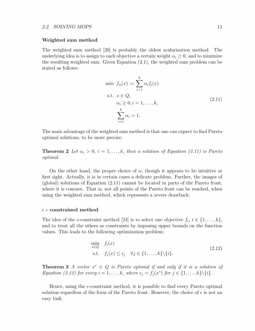
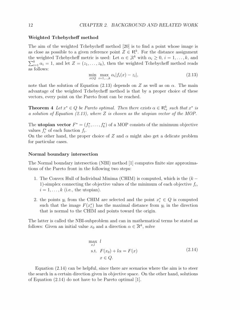
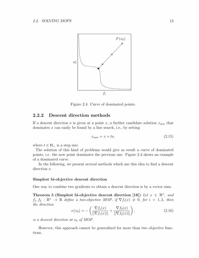
Figure 2.4: Curve of dominated points.
2.2.2 Descent direction methods
If a descent direction ν is given at a point x, a further candidate solution xnew thatdominates x can easily be found by a line search, i.e., by setting
xnew = x+ tν, (2.15)
where t ∈ R+ is a step size.The solution of this kind of problems would give as result a curve of dominated
points, i.e. the new point dominates the previous one. Figure 2.4 shows an exampleof a dominated curve.
In the following, we present several methods which use this idea to find a descentdirection ν.
Simplest bi-objective descent direction
One way to combine two gradients to obtain a descent direction is by a vector sum.
Theorem 5 (Simplest bi-objective descent direction [18]) Let x ∈ Rn, andf1, f2 : Rn → R define a two-objective MOP. if ∇fi(x) 6= 0, for i = 1, 2, thenthe direction
ν(x0) = −(∇f1(x)
||∇f1(x)||+∇f2(x)
||∇f2(x)||
), (2.16)
is a descent direction at x0 of MOP.
However, this approach cannot be generalized for more than two objective func-tions.
14 CHAPTER 2. BACKGROUND AND RELATED WORK
Directed search
The directed search method [17] allows to steer the search from a given point x ∈ Qinto a desired direction d ∈ Rk. A direction vector ν ∈ Rn can be computed suchthat
limt←0
fi(x0 + tv)− fi(x0)t
= di, i = 1, . . . k. (2.17)
In the following, we describe two methods that use this idea. The first one is a descentmethod that steers in a given direction d. The second one is a continuation methodwith the particular advantage that this method does not require any second gradientinformation in contrast to other methods [5, 6].
Descent method The following idea is proposed. Assume a point x0 ∈ Q is givenas well as a vector d ∈ Rk representing a desired direction in objective space. Thiscan be expressed as follows
J(x)ν = d,
where ν ∈ Rn is a search direction in parameter space and J(x) is the jacobian matrix,which is defined by
J(x) =
∂f1∂x1
(x) · · · ∂f1∂xn
(x)...
. . ....
∂fk∂x1
(x) · · · ∂fk∂xn
(x)
. (2.18)
With this the authors propose that v can be computed by solving a system of linearequations. Since typically the number of parameters is higher than the number ofobjectives, the system of equations is underdetermined, which implies that its solutionis not unique. To deal with this, the problem can be formulated as
ν = J(x0)+d,
where J(x0)+ denotes the pseudo inverse of the Jacobian J(x0) ∈ Rk×n. Further, we
can solve the following initial value problem (IVP):
x(0) = x0 ∈ Rn
x(m) = να(x(m)), t > 0.(2.19)
Continuation method Once an optimal point has been found by the methodabove, this second method performs a movement along the Pareto set of a givenMOP.
Assume we are given a (local) Pareto point x and the convex weight α such that
k∑i=1
αi∇fi(x) = 0 (2.20)
and further we assume thatrank(J(x)) = k − 1. (2.21)
2.2. SOLVING MOPS 15
It is known (e.g., [6]) that in this case α is orthogonal to the Pareto front, i.e.,
α⊥TyδF (Rn), (2.22)
where y = F (x) and δF (Rn) denotes the border of the image F (Rn). Thus, a searchorthogonal to α (in objective space) could be promising to obtain new predictorpoints. A QR-factorization of α can be computed to use the method above, i.e.,
α = QR, (2.23)
where Q = (q1, . . . , qk) ∈ Rk×k is an orthogonal matrix and i = 1, . . . , k its columnvectors, and R = (r11, 0, . . . , 0)T ∈ Rk×1 with r11 ∈ R\{0}. Since by Equation (2.23)α = r11q1 and Q orthogonal, it follows that the column vectors q2, . . . , qk build anorthonormal basis of the hyperplane which is orthogonal to α. Thus, a promising setof search directions νi may be the ones which satisfy
J(x)νi = qi, i = 2, . . . , k. (2.24)
Since α is not in the image of J(x) (else x would not be a Pareto point), it follows thatthe vectors q2, . . . , qk are in the image of J(x), i.e., Equation (2.24) can be solved foreach i ∈ {2, . . . , k}. Then, the following can be chosen as the set of predictor direction:
pi = x0 + tνi. (2.25)
Note that by this choice of predictor direction no second derivative of the objectivesare required.
Now, a corrector step can be used. Given a predictor pi ∈ p, we can use pi asinitial value for Equation (2.19) and choosing α0, i.e., the weight from the previoussolution x0 leads to a new solution x1.
Method of Schaffler, Schultz and Weinzierl
The following function is defined [16]:
q(x) =k∑i=1
a∇fi(x),
where q : Rn → Rn and a is a solution of
minα∈Rk
∣∣∣∣∣∣∣∣∣∣k∑i=1
αi∇fi(x)
∣∣∣∣∣∣∣∣∣∣2
2
, αi ≥ 0, i = 1, . . . , k,k∑i=1
αi = 1
,
where ∇fi is the gradient of ith objective function fi.From this we have that either q(x) = 0 or −q(x) is a descent direction for all
the objective functions; hence, each x with q(x) = 0 fulfills the first-order necessaryconditions for Pareto optimality.
16 CHAPTER 2. BACKGROUND AND RELATED WORK
Method of Fliege and Svaiter
The following function is defined [2]:
fx(ν) = max(Av)i, i = 1, . . . , k,
where fx : Rn → R. We can see that fx is convex and positive homogeneous. Usingthis function the authors propose the following problem:
min fx(ν) +1
2||v||2
subject to ν ∈ Rn.
From this we have that, if x is Pareto optimal, then ν(x) = 0. If it is not the casethen ν(x) is a descent direction.
2.2.3 Stochastic methods
An alternative to the classical methods is given by an area known as EvolutionaryMulti-Objective Optimization. This area has developed a wide variety of methods.These methods are known as Multi-Objective Evolutionary Algorithms (MOEAs).Some of their advantages are that they do not require gradient information about theproblem, instead they rely on stochastic search procedures. Another advantage is thatthey give an approximation of the Pareto set and the Pareto front in one execution.Examples of these methods can be found in [12, 13]. One drawback is that MOEAsdo not guarantee convergence towards the Pareto front. In the following we reviewtwo of the most important stochastic methods to solve a MOP and also an approachto find the set of approximate solutions PQ,ε.
Nondominated Sorting Genetic Algorithm II
The Nondominated Sorting Genetic Algorithm II (NSGA-II) was proposed in [25].The NSGA-II has two main mechanisms. The first one is the non-dominated sort,where the idea is to rank the current solutions using the Pareto dominance relation-ship, i.e. the ranking says by how many solutions the current solution is dominated.This helps to identify the best values and to use them to generate new solutions.
The second mechanism is called crowding distance. The idea is to measure thedistance from a given point to its neighbors. This helps to identify the solutions withless distance as it means that there are more solutions in that region.
These components aim to accomplish the goals of convergence and spread respec-tively. Due these mechanisms it has a good overall performance and it has become aprominent method to the point. It is one of the methods against others have to becompared, at least if two and three objectives are considered.
2.2. SOLVING MOPS 17
MOEA based on decomposition
Another prominent algorithm is called MOEA based on decomposition (MOEA/D)which was proposed in [26]. The main idea of this method is to make a decompositionof the original MOP into N SOPs also called subproblems. Then the algorithm solvesthese subproblems using the information from its neighbor subproblems. The decom-position is made by using one of the following methods: Weighted sum, weightedTchebycheff or NBI.
As it is the case of the NSGA-II, this method also gives good results in solvingMOPs and has become one of the most popular algorithms. Also this is one of themethods against others have to be compared.
Evolutionary computation methods for PQ,ε
The methods described above aim for the approximation of the Pareto set and Paretofront, but now the goal is to compute the set of approximate solutions.
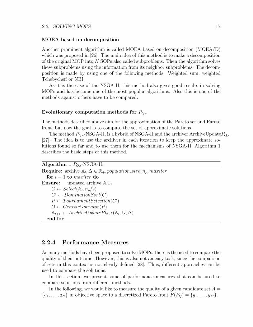
The method PQ,ε-NSGA-II, is a hybrid of NSGA-II and the archiver ArchiveUpdatePQ,ε[27]. The idea is to use the archiver in each iteration to keep the approximate so-lutions found so far and to use them for the mechanisms of NSGA-II. Algorithm 1describes the basic steps of this method.
Algorithm 1 PQ,ε-NSGA-II.
Require: archive Al,∆ ∈ R+, population size, np,maxiterfor i = 1 to maxiter do
Ensure: updated archive Al+1
C ← Select(Al, np/2)C ′ ← DominationSort(C)P ← TournamentSelection(C ′)O ← GeneticOperator(P )Al+1 ← ArchiveUpdatePQ, ε(Al, O,∆)
end for
2.2.4 Performance Measures
As many methods have been proposed to solve MOPs, there is the need to compare thequality of their outcome. However, this is also not an easy task, since the comparisonof sets in this context is not clearly defined [28]. Thus, different approaches can beused to compare the solutions.
In this section, we present some of performance measures that can be used tocompare solutions from different methods.
In the following, we would like to measure the quality of a given candidate set A ={a1, . . . , aN} in objective space to a discretized Pareto front F (PQ) = {y1, . . . , yM}.
18 CHAPTER 2. BACKGROUND AND RELATED WORK
Generational Distance
The generational distance (GD) is used to measure the distance from the candidate setA to the Pareto front F (PQ) [29]. The lower value of GD the better is the candidateset A. A value of zero means, A ∈ F (PQ). However, if an element an element of theset is duplicated then the indicator gives a value closer to zero.
GD(A,F (PQ)) =1
|A|
|A|∑i=1
dist2(ai, F (PQ))p
1p
. (2.26)
To avoid the potential drawback a slight modification was proposed [30].
GD(A,F (PQ))p =
1
|A|
|A|∑i=1
dist2(ai, F (PQ))p
1p
. (2.27)
Inverted Generational Distance
The inverted generational distance (IGD) measures the distance from the Paretofront F (PQ) to the candidate set A [31]. However, this indicator is sensitive to thediscretization of the Pareto front. If a better discretization of the Pareto front is usedthen it will output a value closer to zero.
IGD(A,F (PQ)) =1
|F (PQ)|
|F (PQ)|∑i=1
dist2(yi, A)p
1p
. (2.28)
To avoid the potential drawback a slight modification was proposed [30].
IGD(A,F (PQ))p =
1
|F (PQ)|
|F (PQ)|∑i=1
dist2(yi, A)p
1p
. (2.29)
Delta p
Now, we present the Hausdorff distance dH , which is used to measure the distancebetween sets. Then, we introduce the indicator ∆p, which is used to make our com-parisons in this thesis work.
Definition 6 (Distance between sets [32]) Let u, v ∈ Rn and A,B ⊂ Rn. Themaximum norm distance d∞, the semi-distance dist(·, ·) and the Hausdorff distancedH(·, ·) are defined as follows:
1. d∞ = maxi=1,...,n
|ui − vi|
2.3. DYNAMICAL SYSTEMS 19
2. dist(u,A) = infv∈A
d∞(u, v)
3. dist(B,A) = supu∈B
d∞(u,A)
4. dH(A,B) = max{dist(A,B), dist(B,A)}
It will be assumed that the infinity norm is used unless it is specified otherwise.
Note that for p = ∞, we have ∆∞ = dH , and for finite values of p the distancesin ∆p are averaged. In [30], ∆p is discussed as a performance indicator in context ofPareto front approximations. In that case, the indicator can be viewed as a combi-nation of the slight variations of the GD and the IGD.
2.3 Dynamical Systems
In this section, we first define a dynamical system (Section 2.3.1), and further on thesolution of a dynamical system (Section 2.3.2 and Section 2.3.3). We also present theconcept of the domain of attraction (Section 2.3.4) and finally we look into methodsthat were proposed to perform a global analysis of a given dynamical system (Section2.4).
2.3.1 Formulation of the problem
A dynamical system [15] can be considered to be a model describing the temporalevolution of a system and it is defined as follows:
x = G(x),
where x is a N -dimensional vector and G : RN → RN is, in general, a nonlinear vectorfunction. The evolution of such a dynamical system can be described by a functionof the form:
xm+1 = G(x(m), µ), (2.30)
where x is a N -dimensional vector, m denotes the mapping step, µ is a parametervector, and G is a general nonlinear vector function. In this case ordinary differentialequations can be used to describe the dynamical systems. These are defined as follows:
x = F (x, t, µ); x ∈ Rn, t ∈ R, µ ∈ Rl,
where x is a N -dimensional state vector, t is the time variable, µ is a l-dimensionalparameter vector, and F is a vector-valued function of x, t and µ.
20 CHAPTER 2. BACKGROUND AND RELATED WORK
2.3.2 Fixed point
When the evolution of a dynamical system is made one may find a point that satisfiesthe following:
x∗ = G(x∗, µ).
In this case, x∗ is called a fixed point of Equation (2.30).
2.3.3 Periodic group
A periodic solution of Equation (2.30) of period l is a sequence of l distinct pointsx∗(j), j = 1, 2, . . . , l such that
x∗(o+ 1) = Go(x∗(1), µ), o = 1, 2, . . . , l − 1,
x∗(1) = Gl(x∗(1), µ).(2.31)
We say that there exists a periodic solution of period l. Any of the pointsx∗(j), j = 1, 2, . . . , l, is called a periodic point of period l. One can see that afixed point is a periodic solution with l = 1.
2.3.4 Domain of attraction
We say x∗(j) is an attractor if there exists a neighborhood U of x∗(j) such that forevery open set V ⊃ x∗(j) there is a N ∈ N such that f j(U) ⊂ V for all j ≥ N . Hence,we can restrict ourselves to the closed invariant set x∗(j), and in this case we obtain
x∗(j) =⋂j∈N
Gj(U).
Thus, we can say that all the points in U are attracted by x∗(j) (under iterationof G), and U is called basin of attraction of x∗(j). If U = Rn, then x∗(j) is called theglobal attractor. Several kinds of attractors exists, however, only the ones formed bythe set of periodic solutions will be considered in this work.
2.4 Global Analysis of Dynamical Systems
In this section, we review methods that are used to compute the global propertiesof a dynamical system. We present the simple cell mapping [15], which is useful tocompute global attractors and domains of attraction of a given dynamical system.The other methods that we present are the subdivision techniques [9], which areuseful to compute the global attractors of a given dynamical system.
2.4.1 Discretization of the space
Now, we do not consider the state space as a continuum but rather as a collection ofstate cells, with each cell being taken as a state entity. Because of this, now we needto introduce some basic concepts regarding the new model.

2.4. GLOBAL ANALYSIS OF DYNAMICAL SYSTEMS 21
Cell state space
An N dimensional cell space S [15] is a space whose elements are N -tuples of integers,and each element is called a cell vector or simply a cell, and is denoted by z.
The simplest way to obtain a cell structure over a given Euclidean state space isto construct a cell structure consisting of rectangular parallelepipeds of uniform size.
Cell functions
Let S be the cell state space for a dynamical system and let the discrete time evolutionprocess of the system be such that each cell in a region of interest S0 ⊂ S has a singleimage cell after one mapping step. Such an evolution process is called Simple CellMapping (SCM)
z(n+ 1) = C(z(n), µ), z ∈ ZN , µ ∈ Rl, (2.32)
where C : ZN × Rl → ZN , and µ is a l-dimensional parameter.
Periodic group
A cell z∗ which satisfies z∗ = C(z∗) is said to be an equilibrium cell of the system.Let Cm denote the cell mapping C applied m times with C0 understood to be identitymapping. A sequence of l distinct cells z∗(j), j ∈ l, which satisfies
z∗(m+ 1) = Cm(z∗(1)),m ∈ l − 1, z∗(1) = C l(z∗(1)), (2.33)
is said to constitute a periodic group or P-Group of period l and each of its elementsz∗(j) a periodic cell of period l. One can see that an equilibrium cell is a l = 1periodic group.
Domains of attraction
A cell z is said to be r steps away from a periodic group if r is the minimum positiveinteger such that Cr(z) = z∗(j), where z∗(j) is one of the cells of that periodic group.
The set of all cells, which are r steps or less removed from a periodic group iscalled the r-step domain of attraction for that periodic group. The total domain ofattraction of a periodic group is its r-step domain of attraction with r →∞.
2.4.2 Simple cell mapping
The main idea of this method is based on the fact that the representation of thenumbers in a computer is finite. A number does not only represent the numberrepresented by its digits, but also an infinite neighborhood of numbers given by theprecision of the machine. This does not allow to assume variables to be continuous,due to rounding errors and for this reason it is possible to consider the space as smallhypercubes whose size is given by the machine precision.
22 CHAPTER 2. BACKGROUND AND RELATED WORK
The cell mapping approach [15] proposes to increase this discretization by dividingthe state space into bigger hypercubes. The evolution of the dynamical system is thenreduced to a new function, which is not defined in Rn, but rather on the cell space. Inthis case we restrict ourselves to functions that are strictly deterministically defined.For this case, we have the so-called simple cell mapping method, which is effective toobtain the attractors and basins of attraction of a dynamical system.
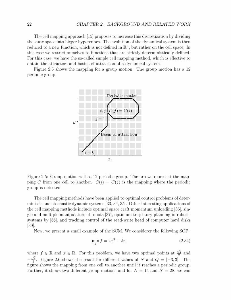
Figure 2.5 shows the mapping for a group motion. The group motion has a 12periodic group.
Figure 2.5: Group motion with a 12 periodic group. The arrows represent the map-ping C from one cell to another. C(i) = C(j) is the mapping where the periodicgroup is detected.
The cell mapping methods have been applied to optimal control problems of deter-ministic and stochastic dynamic systems [33, 34, 35]. Other interesting applications ofthe cell mapping methods include optimal space craft momentum unloading [36], sin-gle and multiple manipulators of robots [37], optimum trajectory planning in roboticsystems by [38], and tracking control of the read-write head of computer hard disks[39].
Now, we present a small example of the SCM. We considerer the following SOP:
minxf = 4x3 − 2x, (2.34)
where f ∈ R and x ∈ R. For this problem, we have two optimal points at√22
and
−√22
. Figure 2.6 shows the result for different values of N and Q = [−3, 3]. Thefigure shows the mapping from one cell to another until it reaches a periodic group.Further, it shows two different group motions and for N = 14 and N = 28, we can

2.4. GLOBAL ANALYSIS OF DYNAMICAL SYSTEMS 23
also see where the domain of attraction of√22
ends and the domain of attraction of
−√22
begins.
0.5 1 1.5 2 2.5N1
(a) N = 2
1 2 3 4N1
(b) N = 4
2 4 6 8 10 12 14N1
(c) N = 14
5 10 15 20 25N1
(d) N = 28
Figure 2.6: Numerical result of the SCM on Equation (2.34) with different grid size,(a) N = 2; (b) N = 4; (c) N = 14; (d) N = 28. The white cells represents the optimalsolutions. The cells with the same color belong to the same domain of attraction (forthose cells their mapping end in the same cell). The arrows represent the cell mapping.Finally, the black curve is the graphic representation of the problem.
2.4.3 Subdivision techniques
The subdivision techniques [9] are based on a generation of a collection of boxes inparameter space, which by the end of the execution covers the periodic groups of agiven dynamical system. Let B0 be an initial collection of finitely many subsets of thecompact set Q such that ∪B∈B0 = Q. Then Bk is obtained from Bk−1 in the followingtwo steps:

24 CHAPTER 2. BACKGROUND AND RELATED WORK
1. Subdivision: Construct from Bk−1 a new system Bk of subsets such that⋃B∈Bk
B =⋃
B∈Bk−1
B
anddiam(Bk) = θkdiam(Bk−1),
where 0 < θmin ≤ θk ≤ θmax < 1.
2. Selection: Define the new collection Bk by
Bk = {B ∈ Bk : there existsB ∈ Bk such that C−1(B) ∩ B 6= 0}.
These methods converge to the periodic group of one (or several) dynamical system(s)in the Hausdorff sense [40]. In the context of optimization this can be the set of globalminimizers [40, 10, 9].
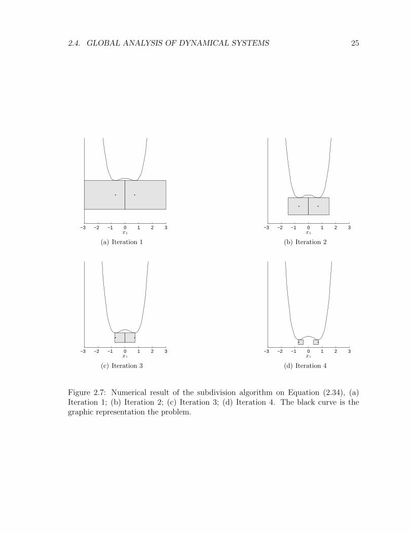
Now, we present a small example of the subdivision techniques on Equation (2.34).We have also chosen Q = [−3, 3]. Figure 2.7 shows the boxes that contain the periodicgroups for different iterations.
2.4. GLOBAL ANALYSIS OF DYNAMICAL SYSTEMS 25
−3 −2 −1 0 1 2 3x1
(a) Iteration 1
−3 −2 −1 0 1 2 3x1
(b) Iteration 2
−3 −2 −1 0 1 2 3x1
(c) Iteration 3
−3 −2 −1 0 1 2 3x1
(d) Iteration 4
Figure 2.7: Numerical result of the subdivision algorithm on Equation (2.34), (a)Iteration 1; (b) Iteration 2; (c) Iteration 3; (d) Iteration 4. The black curve is thegraphic representation the problem.

26 CHAPTER 2. BACKGROUND AND RELATED WORK
Chapter 3
Simple Cell Mapping forMulti-Objective Optimization
In this chapter, we first describe the simple cell mapping method for general dynamicalsystems (Section 3.1). We further adapt the simple cell mapping method to thecontext of multi-objective optimization (Section 3.2) and finally we present numericalresults on academic models and a comparison with NSGA-II and MOEA/D (Section3.4).
3.1 Simple Cell Mapping
In general, when we solve a problem, we do not obtain an exact result. This is eitherdue to the limited machine precision (roundoff errors) or by a limited measurementaccuracy while doing an experiment.
This is the main idea behind the SCM method [15]. Since these problems areunavoidable, the method proposes to increase this error by a given discretization andassumes every value as a discrete quantity.
The SCM method is an useful tool to do a global analysis of a given dynamicalsystem. In this section we present the classical SCM method and describe some ofthe key elements used by the method to capture the global properties of a dynamicalsystem. We also provide an analysis of the simple cell mapping method based ongraph theory.
3.1.1 Description of the SCM Method
The SCM method uses some sets in order to capture the global properties of a cell,which we describe in the following:
• Group motion number (Gr): The group number uniquely identifies a periodicmotion; it is assigned to every periodic cell of that periodic motion and also toevery cell in the domain of attraction. The group numbers, which are positiveintegers, can be assigned sequentially.
27
28 CHAPTER 3. SCM FOR MOO
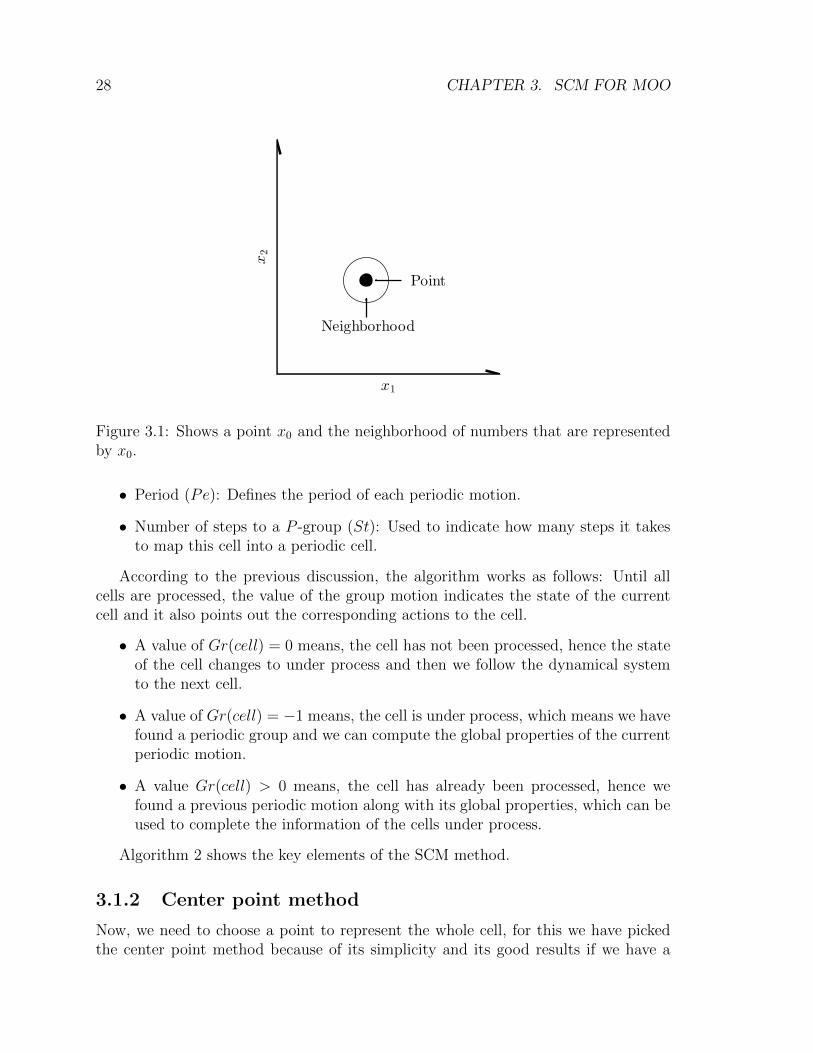
Point
Neighborhood
x1
x2
Figure 3.1: Shows a point x0 and the neighborhood of numbers that are representedby x0.
• Period (Pe): Defines the period of each periodic motion.
• Number of steps to a P -group (St): Used to indicate how many steps it takesto map this cell into a periodic cell.
According to the previous discussion, the algorithm works as follows: Until allcells are processed, the value of the group motion indicates the state of the currentcell and it also points out the corresponding actions to the cell.
• A value of Gr(cell) = 0 means, the cell has not been processed, hence the stateof the cell changes to under process and then we follow the dynamical systemto the next cell.
• A value of Gr(cell) = −1 means, the cell is under process, which means we havefound a periodic group and we can compute the global properties of the currentperiodic motion.
• A value Gr(cell) > 0 means, the cell has already been processed, hence wefound a previous periodic motion along with its global properties, which can beused to complete the information of the cells under process.
Algorithm 2 shows the key elements of the SCM method.
3.1.2 Center point method
Now, we need to choose a point to represent the whole cell, for this we have pickedthe center point method because of its simplicity and its good results if we have a

3.1. SIMPLE CELL MAPPING 29
Figure 3.2: Shows a periodic motion along with its global properties.
fine grid. This method is as follows, given a cell pcell ∈ Z , we compute its centerpcell center ∈ Rn.
When a cell is picked by the SCM method to start the process, a cell numberis given and we need to convert it into its cell center in order to start following thedynamical system.
The first step is to convert the cell number into its cell coordinates ∈ Zn of the cell.If we have the same number of divisions for each dimension i.e. Ni = b, ∀i ∈ n, thenthis problem can be seen as a numerical base conversion (e.g. convert from decimalto binary), where the base is given by N . This problem can be solved by means ofsuccessive divisions.
Now, in order to generalize this process, we can use the same algorithm but ineach step, we change the base, which in this case is given by Ni. Algorithm 3 showsthe realization of this idea.
The next step is to take the cell coordinates and output the center of the cell.This is given by the following expression:
pcell centeri = lbi + hizi −1
2hi, i = 1, . . . , n, (3.1)
where lb is a vector with the lower bound and h is a vector with the size of the cellfor each dimension.
Once we have followed from one cell to another one, we need to compute thecell number of the new cell, which represents the inverse process of the algorithmdescribed above. Given a point ∈ Rn identify in which cell is located. Given the cellcenter ∈ Rn, the cell coordinates ∈ Zn are given by the following expression:
pcelli = round((cell centeri − lbi)/hi + 1/2), i = 1 . . . , n. (3.2)
30 CHAPTER 3. SCM FOR MOO
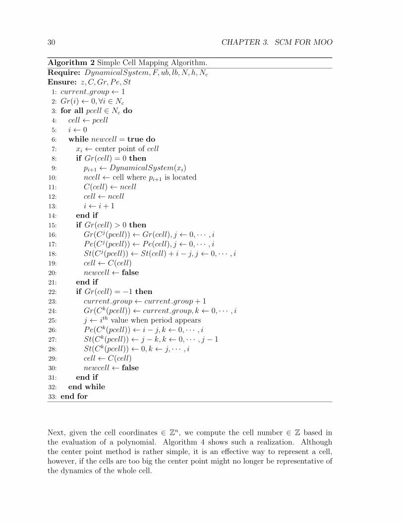
Algorithm 2 Simple Cell Mapping Algorithm.
Require: DynamicalSystem, F, ub, lb, N, h,Nc
Ensure: z, C,Gr, Pe, St1: current group← 12: Gr(i)← 0,∀i ∈ Nc
3: for all pcell ∈ Nc do4: cell← pcell5: i← 06: while newcell = true do7: xi ← center point of cell8: if Gr(cell) = 0 then9: pi+1 ← DynamicalSystem(xi)
10: ncell← cell where pi+1 is located11: C(cell)← ncell12: cell← ncell13: i← i+ 114: end if15: if Gr(cell) > 0 then16: Gr(Cj(pcell))← Gr(cell), j ← 0, · · · , i17: Pe(Cj(pcell))← Pe(cell), j ← 0, · · · , i18: St(Cj(pcell))← St(cell) + i− j, j ← 0, · · · , i19: cell← C(cell)20: newcell← false21: end if22: if Gr(cell) = −1 then23: current group← current group+ 124: Gr(Ck(pcell))← current group, k ← 0, · · · , i25: j ← ith value when period appears26: Pe(Ck(pcell))← i− j, k ← 0, · · · , i27: St(Ck(pcell))← j − k, k ← 0, · · · , j − 128: St(Ck(pcell))← 0, k ← j, · · · , i29: cell← C(cell)30: newcell← false31: end if32: end while33: end for
Next, given the cell coordinates ∈ Zn, we compute the cell number ∈ Z based inthe evaluation of a polynomial. Algorithm 4 shows such a realization. Althoughthe center point method is rather simple, it is an effective way to represent a cell,however, if the cells are too big the center point might no longer be representative ofthe dynamics of the whole cell.
3.1. SIMPLE CELL MAPPING 31
Center Point
Cell i
Center Point
Cell jTransition
x1
x2
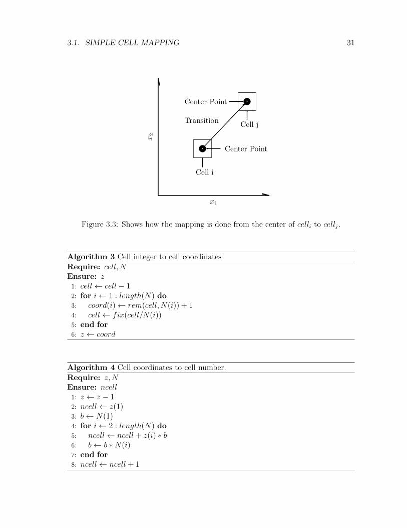
Figure 3.3: Shows how the mapping is done from the center of celli to cellj.
Algorithm 3 Cell integer to cell coordinates
Require: cell, NEnsure: z
1: cell← cell − 12: for i← 1 : length(N) do3: coord(i)← rem(cell, N(i)) + 14: cell← fix(cell/N(i))5: end for6: z ← coord
Algorithm 4 Cell coordinates to cell number.
Require: z,NEnsure: ncell
1: z ← z − 12: ncell← z(1)3: b← N(1)4: for i← 2 : length(N) do5: ncell← ncell + z(i) ∗ b6: b← b ∗N(i)7: end for8: ncell← ncell + 1
32 CHAPTER 3. SCM FOR MOO
3.1.3 Analysis of SCM
The SCM method can be viewed as a graph problem g = (x, e), where x is the set ofvertex of the graph and e is the set of edges. In the following we describe the SCMas a graph problem.
1. Create graph: The first step consists of creating a graph g. The vector x isequal to the set S of cells. The vector e is the mapping of a cell i to a cell j,i.e. for a cell i compute its center point and then follow the dynamical systemto a cell j. Which is the representation of the transition between vertexes.
2. Find cycles: The second step is to use the graph g to compute the globalproperties of the dynamical system. For this we could use either breadth searchfirst or deep search first (both methods are equivalent in this case, since we onlyhave transition for each vertex) and these methods can also give us the size ofthe cycles if we use the colored version of the algorithms.
This view of the SCM method helps us to study the method in terms of space andtime complexity. In the following, we state some of the more important properties ofthe method.
• The out-degree [41] of the graph g is 1.
• The generation of the graph is done in O(|x|), since for each vertex we onlyhave one edge going out.
• The search for cycles is done in O(|x|+ |e|), since each vertex and edge is visitedonce.
• If we use an adjacency list representation for the graph g, O(|x| + |e|) is thememory needed to store the graph.
• The number of vertexes x is given by N1×N2× . . . Nn, which is exponential inthe number of dimensions. This is the weakest point of the SCM method, thusthe method is restricted to low dimensional problems.
3.2 Adapting the SCM Method for MOPs
So far, the SCM method is designed for general dynamical systems as shown inAlgorithm 2. In order to apply it to the context of multi-objective optimization, wehave to define a suitable dynamical system. For this, we have chosen to take modelsthat are derived from descent direction methods.
3.2. ADAPTING THE SCM METHOD FOR MOPS 33
3.2.1 Dynamical system
In this section, we have picked the descent direction from [18] to be used with theSCM method. Using Equation (2.16), the dynamical system
x(t) = v(x(t)) (3.3)
can now be used since it defines a pressure toward the Pareto set/front of the MOPat hand. The other descent direction methods described previously can be used in asimilar form.
3.2.2 Step size control
Once we have decided which descent direction ν to use, we are left with the problemof choosing an appropriate step length t.
Typically, the computation of the step size is not easy as we have two conflictingwishes. First, we would like to choose a step size t that lowers the objective functionas much as possible with a given descent direction ν. Ideally, we would like to havethe global minimizer of the function
φ(t) = F (x+ tν), t > 0, (3.4)
however, doing this we would spend a lot of function evaluation solving this problemand this is in contrast to the second wish, which is to make this decision as cheap aspossible in terms of time and number of function evaluations.
As an alternative to the global minimizer of the function φ, we can use an inexactstep size control as the ones proposed in [2, 42].
In the particular case of the SCM for multi-objective optimization, it has severaladvantages for solving the step size control problem since it has more information athand. For instance, we have the size of the cell which is given by h and we also havethat we start at the center of each cell. With this information, we already have a valuefor sufficient decrease. If there exists a tνi ≥ hi
2, i = 1, . . . , n, then we ensure that we
leave the current cell, which it is what the SCM method needs to keep working.Now, to decide if the step size t is accepted, we can use a dominance test, if the
image of the new point F (xi+1) ≺ F (xi) then we accept the step size t else we can usebacktracking until we find an appropriate step size or the step size is so small that itwould be enough to leave the current cell.
We are left with the choice of the initial step size t0. For this we could choosean arbitrary initial value and if this value is not accepted, we could rely in the back-tracking to help us find an appropriate value for t0. However we can also computethe nearest neighbor given the descent direction ν from the current cell center. Thisidea is shown in Equation (3.5).
t0 = max
(hiνi
)+ ε, ∀i|νi 6= 0. (3.5)
34 CHAPTER 3. SCM FOR MOO
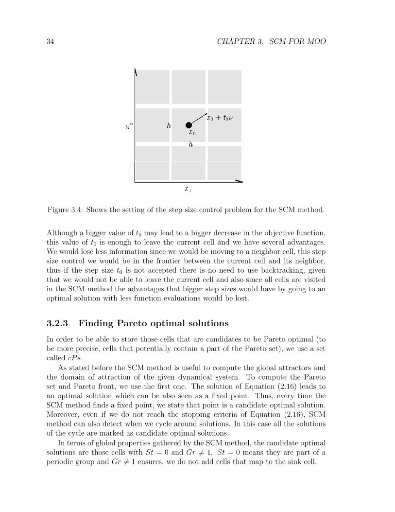
Figure 3.4: Shows the setting of the step size control problem for the SCM method.
Although a bigger value of t0 may lead to a bigger decrease in the objective function,this value of t0 is enough to leave the current cell and we have several advantages.We would lose less information since we would be moving to a neighbor cell, this stepsize control we would be in the frontier between the current cell and its neighbor,thus if the step size t0 is not accepted there is no need to use backtracking, giventhat we would not be able to leave the current cell and also since all cells are visitedin the SCM method the advantages that bigger step sizes would have by going to anoptimal solution with less function evaluations would be lost.
3.2.3 Finding Pareto optimal solutions
In order to be able to store those cells that are candidates to be Pareto optimal (tobe more precise, cells that potentially contain a part of the Pareto set), we use a setcalled cPs.
As stated before the SCM method is useful to compute the global attractors andthe domain of attraction of the given dynamical system. To compute the Paretoset and Pareto front, we use the first one. The solution of Equation (2.16) leads toan optimal solution which can be also seen as a fixed point. Thus, every time theSCM method finds a fixed point, we state that point is a candidate optimal solution.Moreover, even if we do not reach the stopping criteria of Equation (2.16), SCMmethod can also detect when we cycle around solutions. In this case all the solutionsof the cycle are marked as candidate optimal solutions.
In terms of global properties gathered by the SCM method, the candidate optimalsolutions are those cells with St = 0 and Gr 6= 1. St = 0 means they are part of aperiodic group and Gr 6= 1 ensures, we do not add cells that map to the sink cell.
3.3. DESCRIPTION THE SCM METHOD FOR MOPS 35
It is important to notice that because of the dynamical system periodic groupswith size greater than 1 should not appear, however, due to discretization errorsand too large step sizes periodic groups greater than 1 may be generated (i.e., anoscillation around the Pareto set can occur). Thus, cells that are involved in thecurrent periodic group are also considered to be candidates.
Now, we have all the elements needed to solve a MOP by means of SCM method.
3.3 Description the SCM method for MOPs
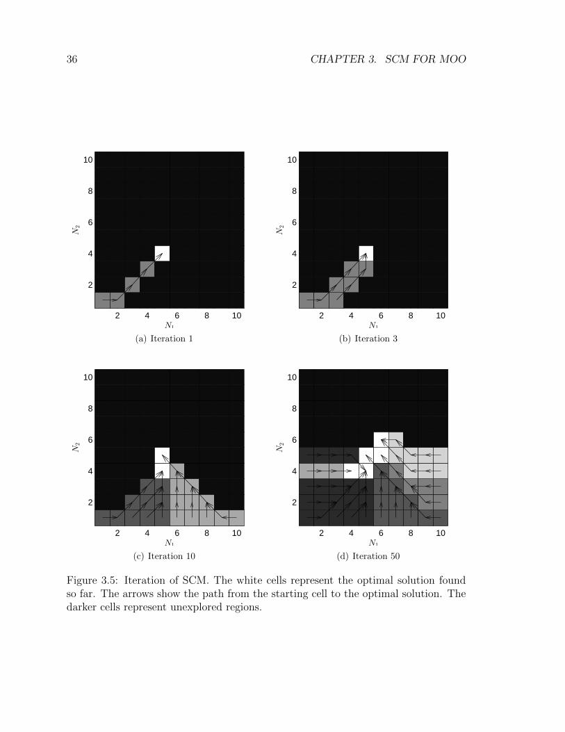
In this section, we put together all the above discussion to write the SCM methodfor multi-objective optimization. Algorithm 5 shows the key elements of the SCMmethod for multi-objective optimization.
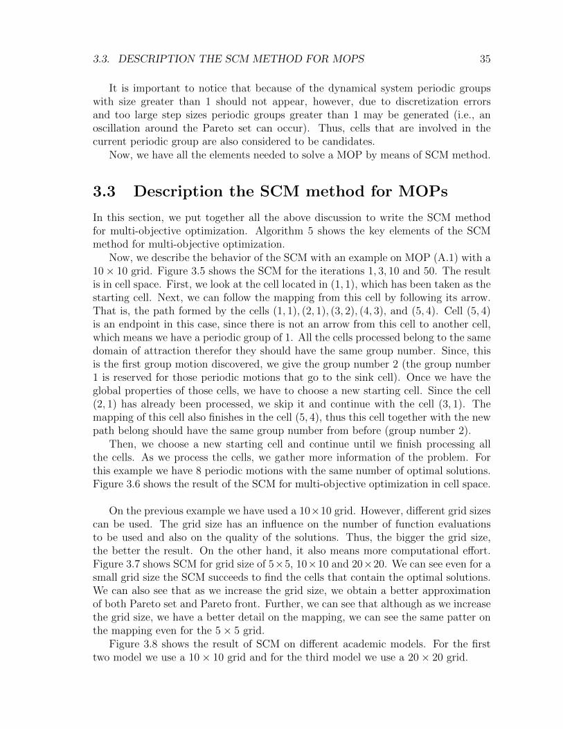
Now, we describe the behavior of the SCM with an example on MOP (A.1) with a10× 10 grid. Figure 3.5 shows the SCM for the iterations 1, 3, 10 and 50. The resultis in cell space. First, we look at the cell located in (1, 1), which has been taken as thestarting cell. Next, we can follow the mapping from this cell by following its arrow.That is, the path formed by the cells (1, 1), (2, 1), (3, 2), (4, 3), and (5, 4). Cell (5, 4)is an endpoint in this case, since there is not an arrow from this cell to another cell,which means we have a periodic group of 1. All the cells processed belong to the samedomain of attraction therefor they should have the same group number. Since, thisis the first group motion discovered, we give the group number 2 (the group number1 is reserved for those periodic motions that go to the sink cell). Once we have theglobal properties of those cells, we have to choose a new starting cell. Since the cell(2, 1) has already been processed, we skip it and continue with the cell (3, 1). Themapping of this cell also finishes in the cell (5, 4), thus this cell together with the newpath belong should have the same group number from before (group number 2).
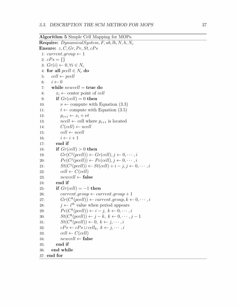
Then, we choose a new starting cell and continue until we finish processing allthe cells. As we process the cells, we gather more information of the problem. Forthis example we have 8 periodic motions with the same number of optimal solutions.Figure 3.6 shows the result of the SCM for multi-objective optimization in cell space.
On the previous example we have used a 10×10 grid. However, different grid sizescan be used. The grid size has an influence on the number of function evaluationsto be used and also on the quality of the solutions. Thus, the bigger the grid size,the better the result. On the other hand, it also means more computational effort.Figure 3.7 shows SCM for grid size of 5×5, 10×10 and 20×20. We can see even for asmall grid size the SCM succeeds to find the cells that contain the optimal solutions.We can also see that as we increase the grid size, we obtain a better approximationof both Pareto set and Pareto front. Further, we can see that although as we increasethe grid size, we have a better detail on the mapping, we can see the same patter onthe mapping even for the 5× 5 grid.
Figure 3.8 shows the result of SCM on different academic models. For the firsttwo model we use a 10× 10 grid and for the third model we use a 20× 20 grid.
36 CHAPTER 3. SCM FOR MOO
2 4 6 8 10
2
4
6
8
10
N1
N2
(a) Iteration 1
2 4 6 8 10
2
4
6
8
10
N1
N2
(b) Iteration 3
2 4 6 8 10
2
4
6
8
10
N1
N2
(c) Iteration 10
2 4 6 8 10
2
4
6
8
10
N1
N2
(d) Iteration 50
Figure 3.5: Iteration of SCM. The white cells represent the optimal solution foundso far. The arrows show the path from the starting cell to the optimal solution. Thedarker cells represent unexplored regions.
3.3. DESCRIPTION THE SCM METHOD FOR MOPS 37
Algorithm 5 Simple Cell Mapping for MOPs.
Require: DynamicalSystem, F, ub, lb, N, h,Nc
Ensure: z, C,Gr, Pe, St, cPs1: current group← 12: cPs = {}3: Gr(i)← 0,∀i ∈ Nc
4: for all pcell ∈ Nc do5: cell← pcell6: i← 07: while newcell = true do8: xi ← center point of cell9: if Gr(cell) = 0 then
10: ν ← compute with Equation (3.3)11: t← compute with Equation (3.5)12: pi+1 ← xi + νt13: ncell← cell where pi+1 is located14: C(cell)← ncell15: cell← ncell16: i← i+ 117: end if18: if Gr(cell) > 0 then19: Gr(Cj(pcell))← Gr(cell), j ← 0, · · · , i20: Pe(Cj(pcell))← Pe(cell), j ← 0, · · · , i21: St(Cj(pcell))← St(cell) + i− j, j ← 0, · · · , i22: cell← C(cell)23: newcell← false24: end if25: if Gr(cell) = −1 then26: current group← current group+ 127: Gr(Ck(pcell))← current group, k ← 0, · · · , i28: j ← ith value when period appears29: Pe(Ck(pcell))← i− j, k ← 0, · · · , i30: St(Ck(pcell))← j − k, k ← 0, · · · , j − 131: St(Ck(pcell))← 0, k ← j, · · · , i32: cPs← cPs ∪ cellk, k ← j, · · · , i33: cell← C(cell)34: newcell← false35: end if36: end while37: end for
38 CHAPTER 3. SCM FOR MOO
2 4 6 8 10
2
4
6
8
10
N1
N2
Figure 3.6: SCM on MOP (A.1) in page 81 with a 10× 10 grid. White cells representoptimal solutions. Further, cells with the same color belong to the same domain ofattraction. Finally, the arrows represent the mapping between cells.
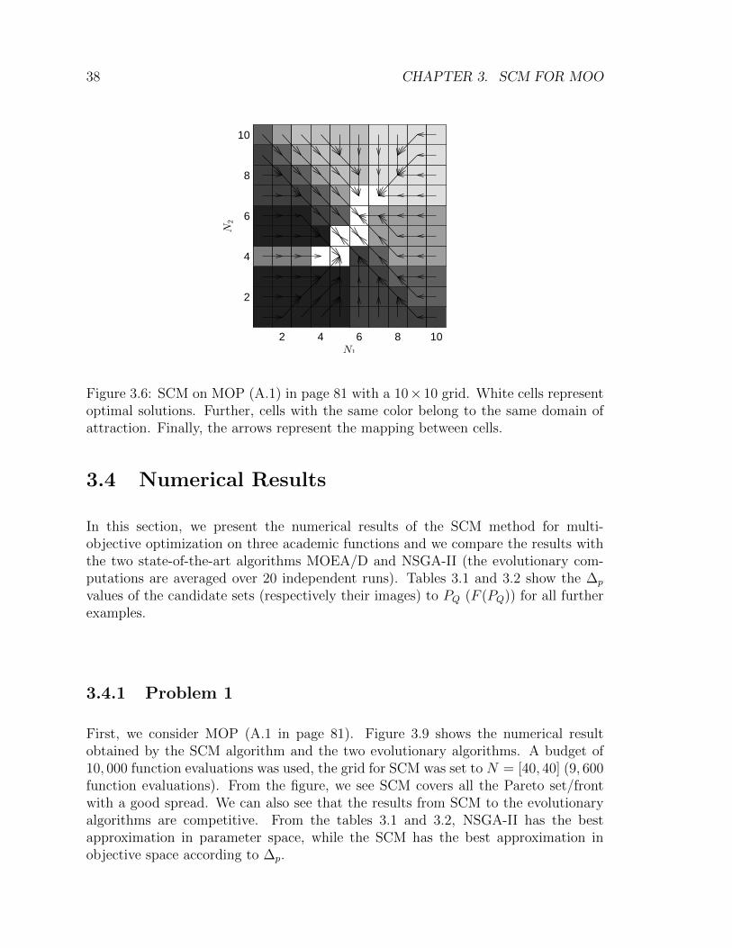
3.4 Numerical Results
In this section, we present the numerical results of the SCM method for multi-objective optimization on three academic functions and we compare the results withthe two state-of-the-art algorithms MOEA/D and NSGA-II (the evolutionary com-putations are averaged over 20 independent runs). Tables 3.1 and 3.2 show the ∆p
values of the candidate sets (respectively their images) to PQ (F (PQ)) for all furtherexamples.
3.4.1 Problem 1
First, we consider MOP (A.1 in page 81). Figure 3.9 shows the numerical resultobtained by the SCM algorithm and the two evolutionary algorithms. A budget of10, 000 function evaluations was used, the grid for SCM was set to N = [40, 40] (9, 600function evaluations). From the figure, we see SCM covers all the Pareto set/frontwith a good spread. We can also see that the results from SCM to the evolutionaryalgorithms are competitive. From the tables 3.1 and 3.2, NSGA-II has the bestapproximation in parameter space, while the SCM has the best approximation inobjective space according to ∆p.

3.4. NUMERICAL RESULTS 39
3.4.2 Problem 2
Next, we consider MOP (A.2 in page 82). Figure 3.10 shows some numerical results.A budget of 10, 000 function evaluations was used, the grid for SCM was N = [40, 40](9, 600 function evaluations). From the figure, we see the SCM method does not onlyfinds the global optimal solution, but also the 8 regions that are nearly optimal, whichis a potential drawback of the method, since in this case we are only interested inglobal optimal solutions. From the tables, MOEA/D has the best approximation inparameter space, while the NSGA-II has the best approximation in objective spaceaccording to ∆p. In this case, since SCM computes also the local optimal solutionsthe ∆p values are not as good as the ones from the evolutionary algorithms.
3.4.3 Problem 3
Further, we consider MOP (A.3 in page 83). Figure 3.11 shows a numerical resultof the SCM and the evolutionary strategies for n = 3. A budget of 10, 000 func-tion evaluations was used, the grid for SCM was N = [10, 10, 10] (6, 000 functionevaluations). Figure 3.12 shows a numerical result of the SCM and the evolutionarystrategies for n = 5. A budget of 600, 000 function evaluations was used, the grid forSCM was N = [10, 10, 10, 10, 10] (600, 000 function evaluations). From the figure, wesee the SCM method is the only one that finds the four components of the Paretoset. We also see the SCM computes a good approximation of the Pareto front Fromthe tables, SCM has the best approximation in parameter space, while the NSGA-IIhas the best approximation in objective space according to ∆p.
3.4.4 Problem 4
Now, we consider MOP (A.6). Figure 3.13 shows a numerical result of the SCM andthe evolutionary strategies. A budget of 6, 000 function evaluations was used, thegrid for SCM was N = [20, 10, 5] (6, 000 function evaluations). For n = 3, we see theSCM method together with NSGA-II yield the best results for this problem. Fromthe tables, SCM has the best approximation in parameter space, while the NSGA-IIhas the best approximation in objective space according to ∆p. For n = 5, SCM isstill able to compute the sets of interest, however the computational cost increasesexponentially as we increase the number of parameters.
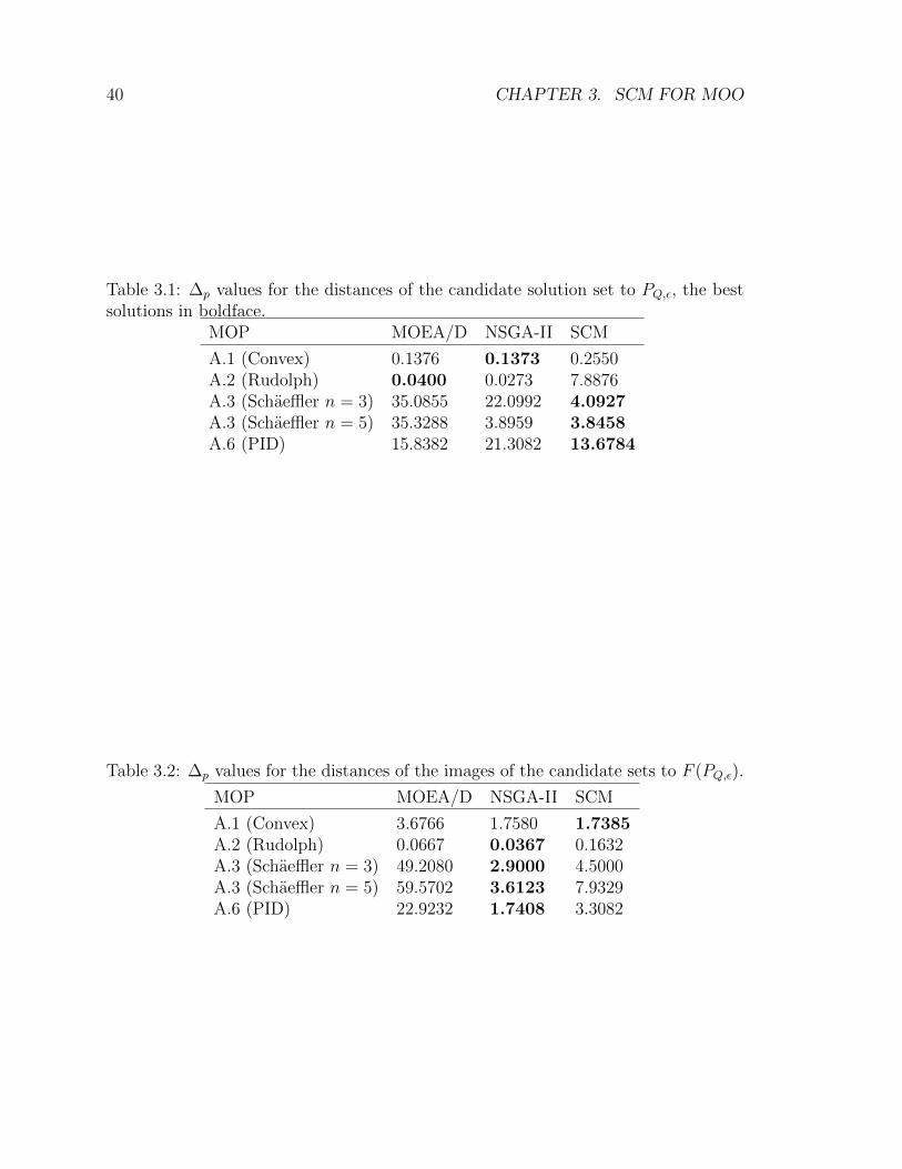
40 CHAPTER 3. SCM FOR MOO
Table 3.1: ∆p values for the distances of the candidate solution set to PQ,ε, the bestsolutions in boldface.
MOP MOEA/D NSGA-II SCM
A.1 (Convex) 0.1376 0.1373 0.2550A.2 (Rudolph) 0.0400 0.0273 7.8876A.3 (Schaeffler n = 3) 35.0855 22.0992 4.0927A.3 (Schaeffler n = 5) 35.3288 3.8959 3.8458A.6 (PID) 15.8382 21.3082 13.6784
Table 3.2: ∆p values for the distances of the images of the candidate sets to F (PQ,ε).
MOP MOEA/D NSGA-II SCM
A.1 (Convex) 3.6766 1.7580 1.7385A.2 (Rudolph) 0.0667 0.0367 0.1632A.3 (Schaeffler n = 3) 49.2080 2.9000 4.5000A.3 (Schaeffler n = 5) 59.5702 3.6123 7.9329A.6 (PID) 22.9232 1.7408 3.3082
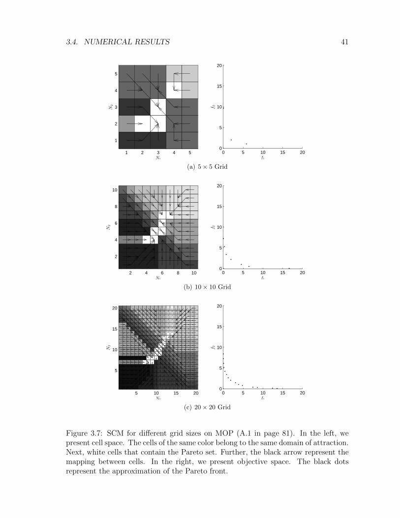
3.4. NUMERICAL RESULTS 41
1 2 3 4 5
1
2
3
4
5
N1
N2
0 5 10 15 200
5
10
15
20
f1
f2
(a) 5× 5 Grid
2 4 6 8 10
2
4
6
8
10
N1
N2
0 5 10 15 200
5
10
15
20
f1
f2
(b) 10× 10 Grid
5 10 15 20
5
10
15
20
N1
N2
0 5 10 15 200
5
10
15
20
f1
f2
(c) 20× 20 Grid
Figure 3.7: SCM for different grid sizes on MOP (A.1 in page 81). In the left, wepresent cell space. The cells of the same color belong to the same domain of attraction.Next, white cells that contain the Pareto set. Further, the black arrow represent themapping between cells. In the right, we present objective space. The black dotsrepresent the approximation of the Pareto front.
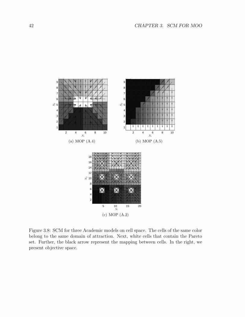
42 CHAPTER 3. SCM FOR MOO
2 4 6 8 10
1
2
3
4
5
6
7
8
9
N1
N2
(a) MOP (A.4)
2 4 6 8 10
1
2
3
4
5
6
7
8
9
N1
N2
(b) MOP (A.5)
5 10 15 20
2
4
6
8
10
12
14
16
18
N1
N2
(c) MOP (A.2)
Figure 3.8: SCM for three Academic models on cell space. The cells of the same colorbelong to the same domain of attraction. Next, white cells that contain the Paretoset. Further, the black arrow represent the mapping between cells. In the right, wepresent objective space.
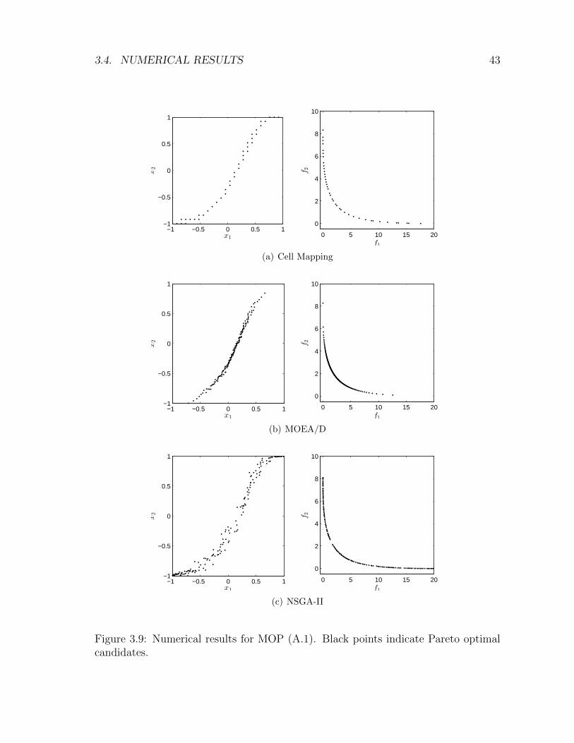
3.4. NUMERICAL RESULTS 43
−1 −0.5 0 0.5 1−1
−0.5
0
0.5
1
x1
x2
0 5 10 15 20
0
2
4
6
8
10
f1
f2
(a) Cell Mapping
−1 −0.5 0 0.5 1−1
−0.5
0
0.5
1
x1
x2
0 5 10 15 20
0
2
4
6
8
10
f1
f2
(b) MOEA/D
−1 −0.5 0 0.5 1−1
−0.5
0
0.5
1
x1
x2
0 5 10 15 20
0
2
4
6
8
10
f1
f2
(c) NSGA-II
Figure 3.9: Numerical results for MOP (A.1). Black points indicate Pareto optimalcandidates.
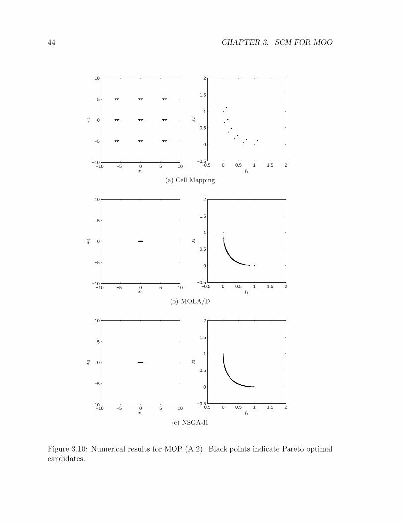
44 CHAPTER 3. SCM FOR MOO
−10 −5 0 5 10−10
−5
0
5
10
x1
x2
−0.5 0 0.5 1 1.5 2−0.5
0
0.5
1
1.5
2
f1
f2
(a) Cell Mapping
−10 −5 0 5 10−10
−5
0
5
10
x1
x2
−0.5 0 0.5 1 1.5 2−0.5
0
0.5
1
1.5
2
f1
f2
(b) MOEA/D
−10 −5 0 5 10−10
−5
0
5
10
x1
x2
−0.5 0 0.5 1 1.5 2−0.5
0
0.5
1
1.5
2
f1
f2
(c) NSGA-II
Figure 3.10: Numerical results for MOP (A.2). Black points indicate Pareto optimalcandidates.
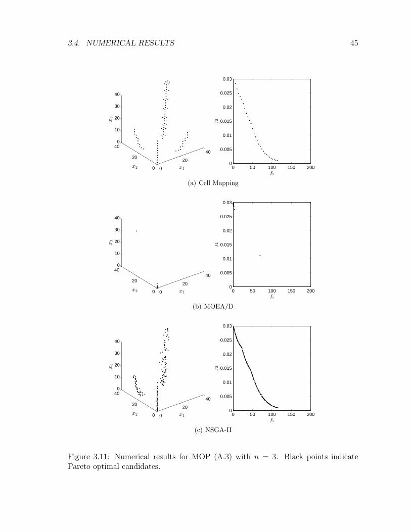
3.4. NUMERICAL RESULTS 45
0
20
40
0
20
400
10
20
30
40
x1x2
x3
0 50 100 150 2000
0.005
0.01
0.015
0.02
0.025
0.03
f1
f2
(a) Cell Mapping
0
20
40
0
20
400
10
20
30
40
x1x2
x3
0 50 100 150 2000
0.005
0.01
0.015
0.02
0.025
0.03
f1
f2
(b) MOEA/D
0
20
40
0
20
400
10
20
30
40
x1x2
x3
0 50 100 150 2000
0.005
0.01
0.015
0.02
0.025
0.03
f1
f2
(c) NSGA-II
Figure 3.11: Numerical results for MOP (A.3) with n = 3. Black points indicatePareto optimal candidates.
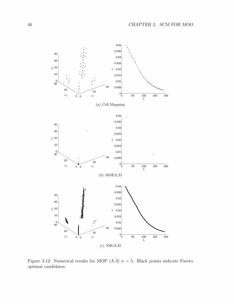
46 CHAPTER 3. SCM FOR MOO
0
20
40
0
20
400
10
20
30
40
x1x2
x3
0 50 100 150 2000
0.005
0.01
0.015
0.02
0.025
0.03
0.035
0.04
f1
f2
(a) Cell Mapping
0
20
40
0
20
400
10
20
30
40
x1x2
x3
0 50 100 150 2000
0.005
0.01
0.015
0.02
0.025
0.03
0.035
0.04
f1
f2
(b) MOEA/D
0
20
40
0
20
400
10
20
30
40
x1x2
x3
0 50 100 150 2000
0.005
0.01
0.015
0.02
0.025
0.03
0.035
0.04
f1
f2
(c) NSGA-II
Figure 3.12: Numerical results for MOP (A.3) n = 5. Black points indicate Paretooptimal candidates.
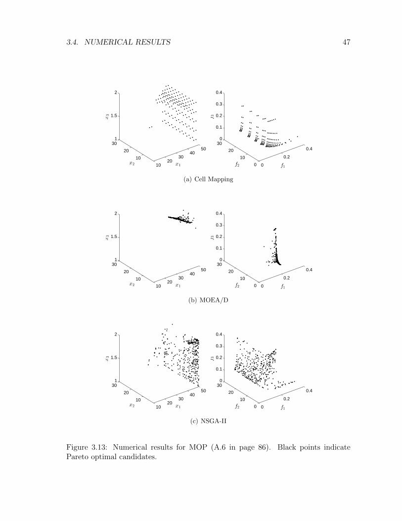
3.4. NUMERICAL RESULTS 47
1020
3040
50
10
20
301
1.5
2
x1x2
x3
0
0.2
0.4
0
10
20
300
0.1
0.2
0.3
0.4
f1f2
f3
(a) Cell Mapping
1020
3040
50
10
20
301
1.5
2
x1x2
x3
0
0.2
0.4
0
10
20
300
0.1
0.2
0.3
0.4
f1f2
f3
(b) MOEA/D
1020
3040
50
10
20
301
1.5
2
x1x2
x3
0
0.2
0.4
0
10
20
300
0.1
0.2
0.3
0.4
f1f2
f3
(c) NSGA-II
Figure 3.13: Numerical results for MOP (A.6 in page 86). Black points indicatePareto optimal candidates.

48 CHAPTER 3. SCM FOR MOO
Chapter 4
Simple Cell Mapping for theApproximation of the Set ofApproximate Solutions
Here we address the problem of computing the set of approximate solutions of a givenMOP. This set is of potential interest for the decision maker (DM) since it might givehim/her additional solutions to the optimal ones for the realization of the projectrelated to the MOP.
In a variety of applications in industry and finance a problem arises that severalobjective functions have to be optimized concurrently leading to multi-objective op-timization problems. For instance, in space mission design, there are two crucial aimsfor the realization of a transfer: Minimization of flight time and fuel consumption ofthe spacecraft [43, 44, 45]. In this case, it makes sense to consider in addition to the‘optimal’ trajectories also approximate solutions since by this the decision maker isoffered a much larger variety of possibilities, and to present one way to compute thisenlarged set of interest with reasonable effort.
As a motivating example, consider the MOP which is a model taken from [27]for the transfer from Earth to Mercury, and the following two points xi with imagesF (xi), i = 1, 2:
x1 = (782, 1288, 1788), F (x1) = (0.462, 1001.7)
x2 = (1222, 1642, 2224), F (x2) = (0.463, 1005.3)
The two objectives are the propellant mass fraction i.e., the portion of the vehicle’smass which does not reach the destination and the flight time (in days). In thedomain, the first parameter is of particular interest: It determines the departuretime from the Earth (in days after 01/01/2000). F (x1) is less than F (x2) in bothcomponents, and thus, x1 can be considered to be ‘better’ than x2. However, notethat the difference in image space is small: the mass fraction of the two solutionsdiffers by 0.001 which makes 0.1% of the total mass, and the flight time differs byfour days for a transfer which takes almost three years. In case the DM is willing to
49
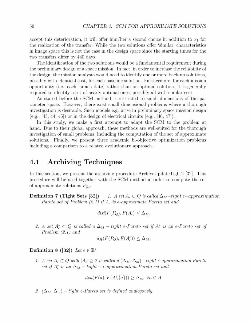
50 CHAPTER 4. SCM FOR APPROXIMATE SOLUTIONS
accept this deterioration, it will offer him/her a second choice in addition to x1 forthe realization of the transfer: While the two solutions offer ‘similar’ characteristicsin image space this is not the case in the design space since the starting times for thetwo transfers differ by 440 days.
The identification of the two solutions would be a fundamental requirement duringthe preliminary design of a space mission. In fact, in order to increase the reliability ofthe design, the mission analysts would need to identify one or more back-up solutions,possibly with identical cost, for each baseline solution. Furthermore, for each missionopportunity (i.e. each launch date) rather than an optimal solution, it is generallyrequired to identify a set of nearly optimal ones, possibly all with similar cost.
As stated before the SCM method is restricted to small dimensions of the pa-rameter space. However, there exist small dimensional problems where a thoroughinvestigation is desirable. Such models e.g. arise in preliminary space mission design(e.g., [43, 44, 45]) or in the design of electrical circuits (e.g., [46, 47]).
In this study, we make a first attempt to adapt the SCM to the problem athand. Due to their global approach, these methods are well-suited for the thoroughinvestigation of small problems, including the computation of the set of approximatesolutions. Finally, we present three academic bi-objective optimization problemsincluding a comparison to a related evolutionary approach.
4.1 Archiving Techniques
In this section, we present the archiving procedure ArchiveUpdateTight2 [32]. Thisprocedure will be used together with the SCM method in order to compute the setof approximate solutions PQε .
Definition 7 (Tight Sets [32]) 1. A set Aε ⊂ Q is called ∆M−tight ε−approximationPareto set of Problem (2.1) if Aε is ε-approximate Pareto set and
dist(F (PQ), F (Aε) ≤ ∆M .
2. A set A∗ε ⊂ Q is called a ∆M − tight ε-Pareto set if A∗ε is an ε-Pareto set ofProblem (2.1) and
dH(F (PQ), F (A∗ε)) ≤ ∆M .
Definition 8 ([32]) Let ε ∈ R∗+
1. A set Aε ⊂ Q with |Aε| ≥ 2 is called a (∆M ,∆m)−tight ε-approximation Paretoset if A∗ε is an ∆M − tight− ε-approximation Pareto set and
dist(F (a), F (A\{a})) ≥ ∆m, ∀a ∈ A.
2. (∆M ,∆m)− tight ε-Pareto set is defined analogously.
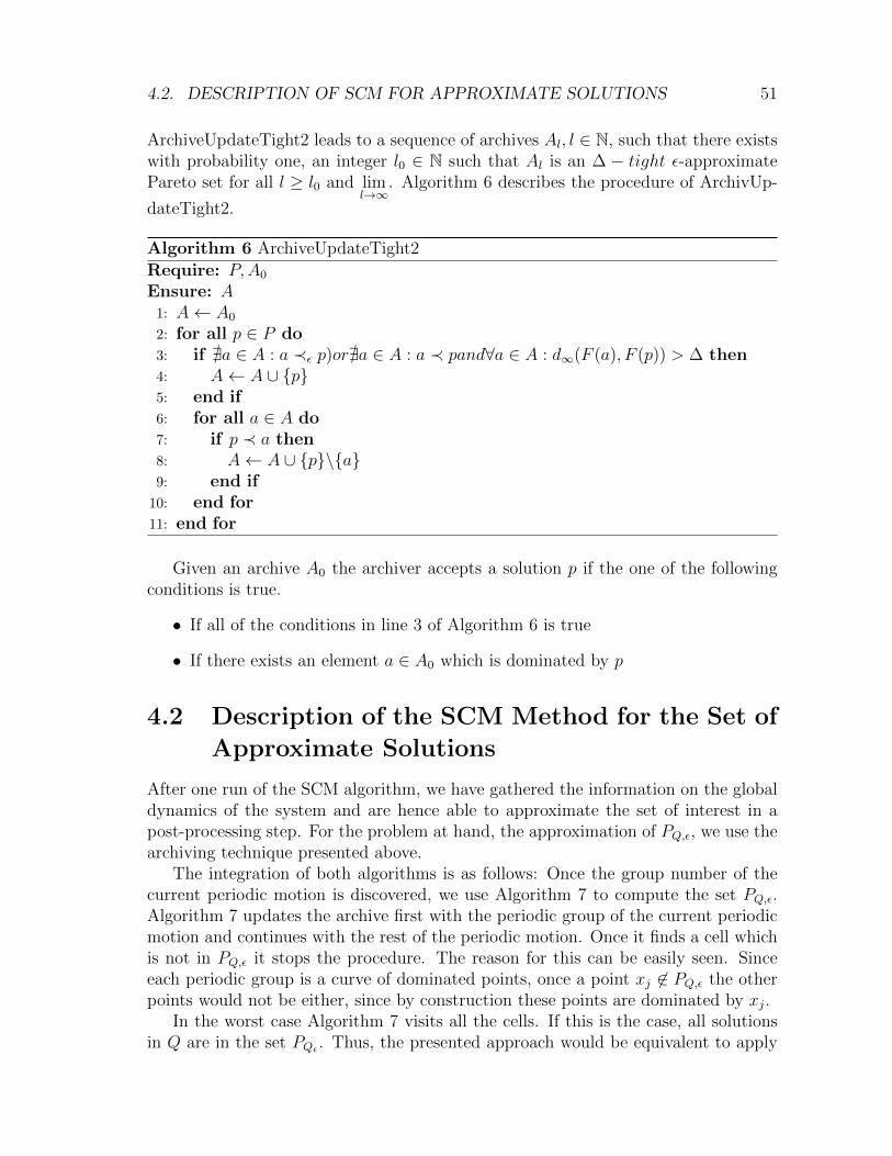
4.2. DESCRIPTION OF SCM FOR APPROXIMATE SOLUTIONS 51
ArchiveUpdateTight2 leads to a sequence of archives Al, l ∈ N, such that there existswith probability one, an integer l0 ∈ N such that Al is an ∆ − tight ε-approximatePareto set for all l ≥ l0 and lim
l→∞. Algorithm 6 describes the procedure of ArchivUp-
dateTight2.
Algorithm 6 ArchiveUpdateTight2
Require: P,A0
Ensure: A1: A← A0
2: for all p ∈ P do3: if @a ∈ A : a ≺ε p)or@a ∈ A : a ≺ pand∀a ∈ A : d∞(F (a), F (p)) > ∆ then4: A← A ∪ {p}5: end if6: for all a ∈ A do7: if p ≺ a then8: A← A ∪ {p}\{a}9: end if
10: end for11: end for
Given an archive A0 the archiver accepts a solution p if the one of the followingconditions is true.
• If all of the conditions in line 3 of Algorithm 6 is true
• If there exists an element a ∈ A0 which is dominated by p
4.2 Description of the SCM Method for the Set of
Approximate Solutions
After one run of the SCM algorithm, we have gathered the information on the globaldynamics of the system and are hence able to approximate the set of interest in apost-processing step. For the problem at hand, the approximation of PQ,ε, we use thearchiving technique presented above.
The integration of both algorithms is as follows: Once the group number of thecurrent periodic motion is discovered, we use Algorithm 7 to compute the set PQ,ε.Algorithm 7 updates the archive first with the periodic group of the current periodicmotion and continues with the rest of the periodic motion. Once it finds a cell whichis not in PQ,ε it stops the procedure. The reason for this can be easily seen. Sinceeach periodic group is a curve of dominated points, once a point xj 6∈ PQ,ε the otherpoints would not be either, since by construction these points are dominated by xj.
In the worst case Algorithm 7 visits all the cells. If this is the case, all solutionsin Q are in the set PQε . Thus, the presented approach would be equivalent to apply
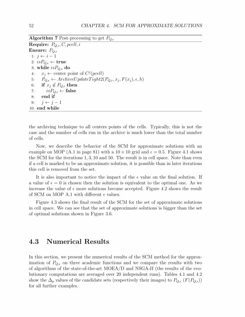
52 CHAPTER 4. SCM FOR APPROXIMATE SOLUTIONS
Algorithm 7 Post-processing to get PQ,εRequire: PQ,ε, C, pcell, iEnsure: PQ,ε
1: j ← i− 12: isPQ,ε ← true3: while isPQ,ε do4: xj ← center point of Cj(pcell)5: PQ,ε ← ArchiveUpdateT ight2(PQ,ε, xj, F (xj), ε, h)6: if xj 6∈ PQ,ε then7: isPQ,ε ← false8: end if9: j ← j − 1
10: end while
the archiving technique to all centers points of the cells. Typically, this is not thecase and the number of cells run in the archive is much lower than the total numberof cells.
Now, we describe the behavior of the SCM for approximate solutions with anexample on MOP (A.1 in page 81) with a 10× 10 grid and ε = 0.5. Figure 4.1 showsthe SCM for the iterations 1, 3, 10 and 50. The result is in cell space. Note than evenif a cell is marked to be an approximate solution, it is possible than in later iterationsthis cell is removed from the set.
It is also important to notice the impact of the ε value on the final solution. Ifa value of ε = 0 is chosen then the solution is equivalent to the optimal one. As weincrease the value of ε more solutions become accepted. Figure 4.2 shows the resultof SCM on MOP A.1 with different ε values.
Figure 4.3 shows the final result of the SCM for the set of approximate solutionsin cell space. We can see that the set of approximate solutions is bigger than the setof optimal solutions shown in Figure 3.6.
4.3 Numerical Results
In this section, we present the numerical results of the SCM method for the approx-imation of PQ,ε on three academic functions and we compare the results with twoof algorithms of the state-of-the-art MOEA/D and NSGA-II (the results of the evo-lutionary computations are averaged over 20 independent runs). Tables 4.1 and 4.2show the ∆p values of the candidate sets (respectively their images) to PQ,ε (F (PQ,ε))for all further examples.
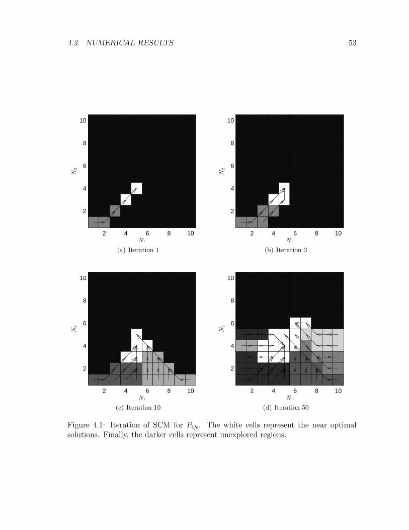
4.3. NUMERICAL RESULTS 53
2 4 6 8 10
2
4
6
8
10
N1
N2
(a) Iteration 1
2 4 6 8 10
2
4
6
8
10
N1
N2
(b) Iteration 3
2 4 6 8 10
2
4
6
8
10
N1
N2
(c) Iteration 10
2 4 6 8 10
2
4
6
8
10
N1
N2
(d) Iteration 50
Figure 4.1: Iteration of SCM for PQε. The white cells represent the near optimalsolutions. Finally, the darker cells represent unexplored regions.
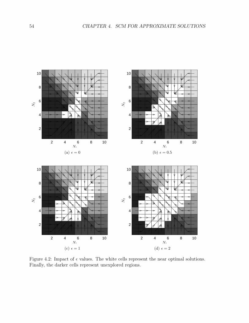
54 CHAPTER 4. SCM FOR APPROXIMATE SOLUTIONS
2 4 6 8 10
2
4
6
8
10
N1
N2
(a) ε = 0
2 4 6 8 10
2
4
6
8
10
N1
N2
(b) ε = 0.5
2 4 6 8 10
2
4
6
8
10
N1
N2
(c) ε = 1
2 4 6 8 10
2
4
6
8
10
N1
N2
(d) ε = 2
Figure 4.2: Impact of ε values. The white cells represent the near optimal solutions.Finally, the darker cells represent unexplored regions.
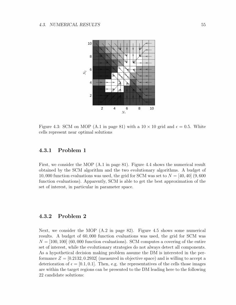
4.3. NUMERICAL RESULTS 55
2 4 6 8 10
2
4
6
8
10
N1
N2
Figure 4.3: SCM on MOP (A.1 in page 81) with a 10 × 10 grid and ε = 0.5. Whitecells represent near optimal solutions
4.3.1 Problem 1
First, we consider the MOP (A.1 in page 81). Figure 4.4 shows the numerical resultobtained by the SCM algorithm and the two evolutionary algorithms. A budget of10, 000 function evaluations was used, the grid for SCM was set to N = [40, 40] (9, 600function evaluations). Apparently, SCM is able to get the best approximation of theset of interest, in particular in parameter space.
4.3.2 Problem 2
Next, we consider the MOP (A.2 in page 82). Figure 4.5 shows some numericalresults. A budget of 60, 000 function evaluations was used, the grid for SCM wasN = [100, 100] (60, 000 function evaluations). SCM computes a covering of the entireset of interest, while the evolutionary strategies do not always detect all components.As a hypothetical decision making problem assume the DM is interested in the per-formance Z = [0.2132, 0.2932] (measured in objective space) and is willing to accept adeterioration of ε = [0.1, 0.1]. Then, e.g. the representatives of the cells those imagesare within the target regions can be presented to the DM leading here to the following22 candidate solutions:
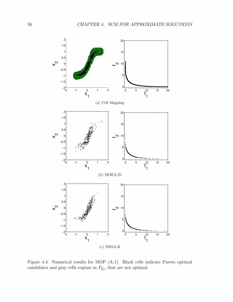
56 CHAPTER 4. SCM FOR APPROXIMATE SOLUTIONS
−2 −1 0 1 2−2
−1.5
−1
−0.5
0
0.5
1
1.5
2
x1
x2
0 5 10 15 20
0
5
10
15
20
f1
f 2
(a) Cell Mapping
−2 −1 0 1 2−2
−1.5
−1
−0.5
0
0.5
1
1.5
2
x1
x2
0 5 10 15 20
0
5
10
15
20
f1
f 2
(b) MOEA/D
−2 −1 0 1 2−2
−1.5
−1
−0.5
0
0.5
1
1.5
2
x1
x2
0 5 10 15 20
0
5
10
15
20
f1
f 2
(c) NSGA-II
Figure 4.4: Numerical results for MOP (A.1). Black cells indicate Pareto optimalcandidates and gray cells regions in PQ,ε that are not optimal.
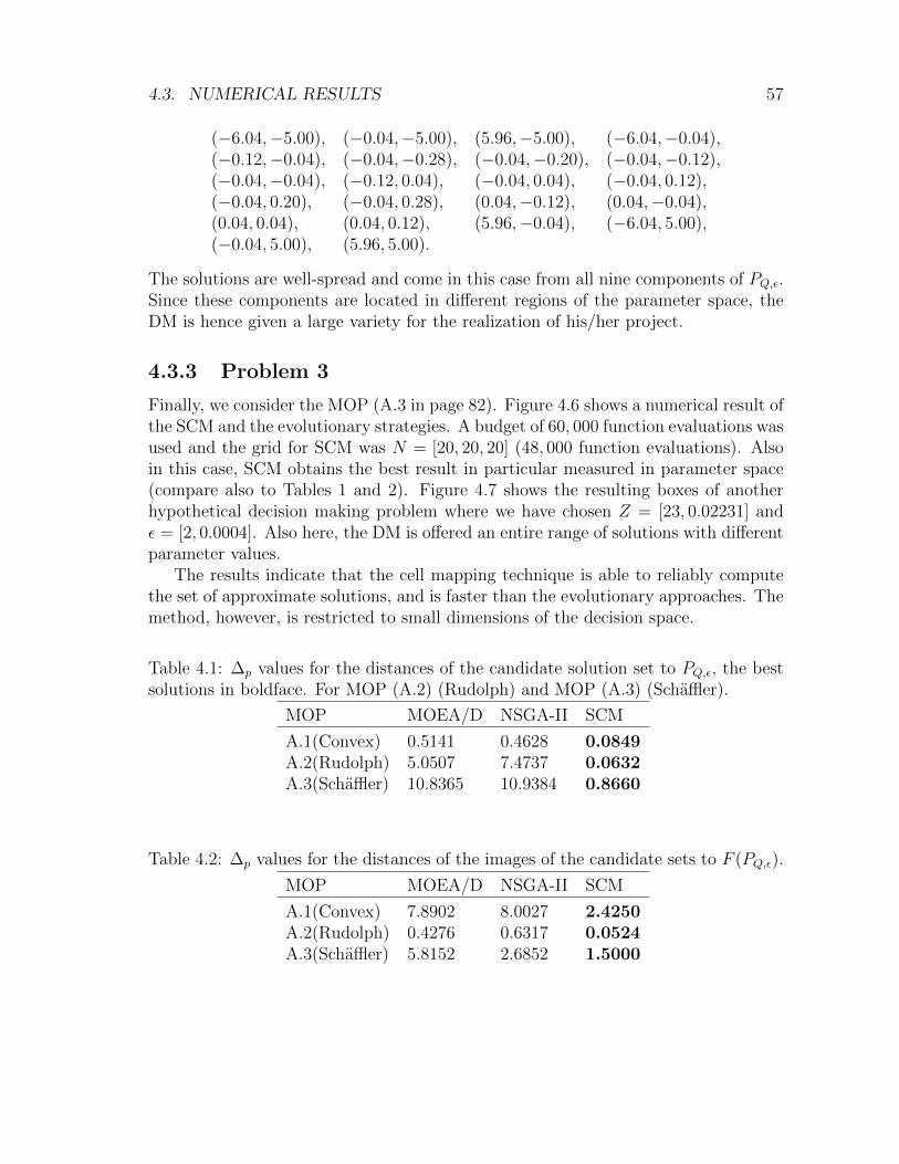
4.3. NUMERICAL RESULTS 57
(−6.04,−5.00), (−0.04,−5.00), (5.96,−5.00), (−6.04,−0.04),(−0.12,−0.04), (−0.04,−0.28), (−0.04,−0.20), (−0.04,−0.12),(−0.04,−0.04), (−0.12, 0.04), (−0.04, 0.04), (−0.04, 0.12),(−0.04, 0.20), (−0.04, 0.28), (0.04,−0.12), (0.04,−0.04),(0.04, 0.04), (0.04, 0.12), (5.96,−0.04), (−6.04, 5.00),(−0.04, 5.00), (5.96, 5.00).
The solutions are well-spread and come in this case from all nine components of PQ,ε.Since these components are located in different regions of the parameter space, theDM is hence given a large variety for the realization of his/her project.
4.3.3 Problem 3
Finally, we consider the MOP (A.3 in page 82). Figure 4.6 shows a numerical result ofthe SCM and the evolutionary strategies. A budget of 60, 000 function evaluations wasused and the grid for SCM was N = [20, 20, 20] (48, 000 function evaluations). Alsoin this case, SCM obtains the best result in particular measured in parameter space(compare also to Tables 1 and 2). Figure 4.7 shows the resulting boxes of anotherhypothetical decision making problem where we have chosen Z = [23, 0.02231] andε = [2, 0.0004]. Also here, the DM is offered an entire range of solutions with differentparameter values.
The results indicate that the cell mapping technique is able to reliably computethe set of approximate solutions, and is faster than the evolutionary approaches. Themethod, however, is restricted to small dimensions of the decision space.
Table 4.1: ∆p values for the distances of the candidate solution set to PQ,ε, the bestsolutions in boldface. For MOP (A.2) (Rudolph) and MOP (A.3) (Schaffler).
MOP MOEA/D NSGA-II SCM
A.1(Convex) 0.5141 0.4628 0.0849A.2(Rudolph) 5.0507 7.4737 0.0632A.3(Schaffler) 10.8365 10.9384 0.8660
Table 4.2: ∆p values for the distances of the images of the candidate sets to F (PQ,ε).
MOP MOEA/D NSGA-II SCM
A.1(Convex) 7.8902 8.0027 2.4250A.2(Rudolph) 0.4276 0.6317 0.0524A.3(Schaffler) 5.8152 2.6852 1.5000
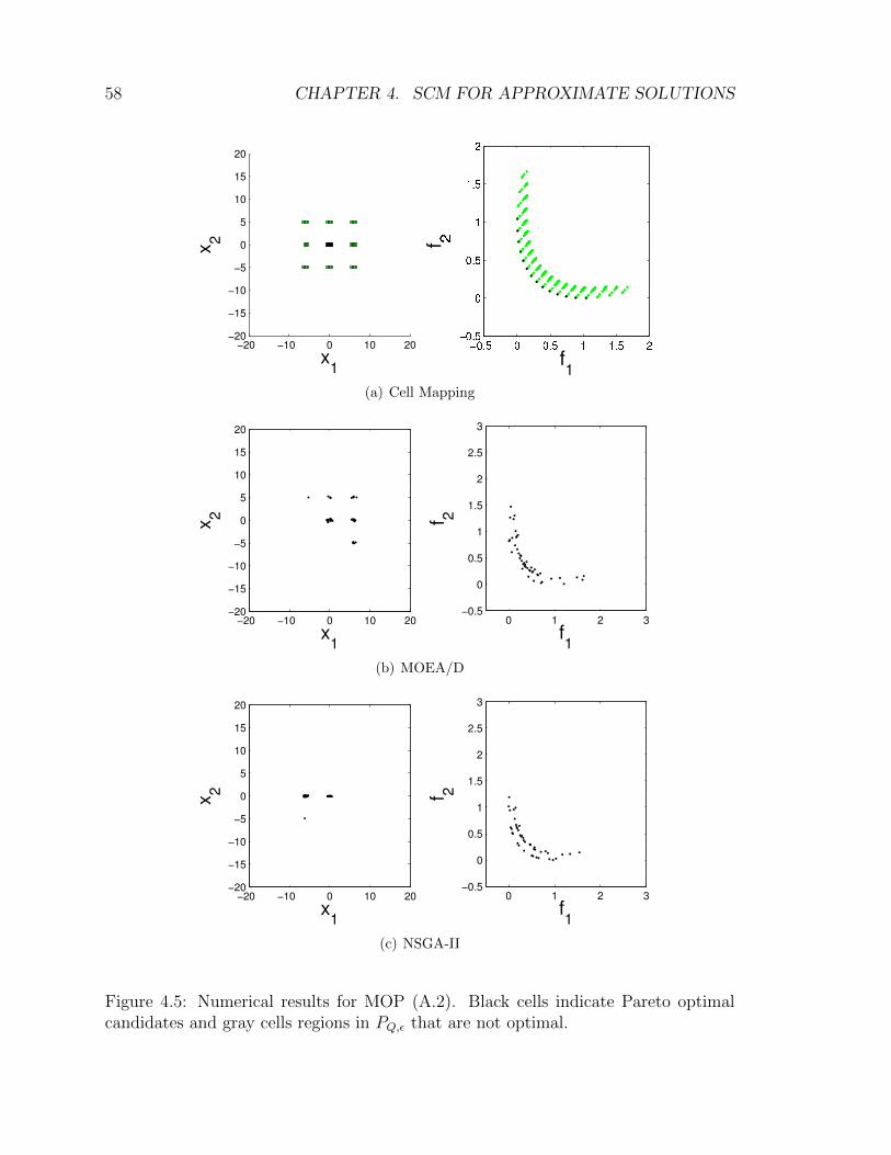
58 CHAPTER 4. SCM FOR APPROXIMATE SOLUTIONS
−20 −10 0 10 20−20
−15
−10
−5
0
5
10
15
20
x1
x2
(a) Cell Mapping
−20 −10 0 10 20−20
−15
−10
−5
0
5
10
15
20
x1
x2
0 1 2 3−0.5
0
0.5
1
1.5
2
2.5
3
f1
f 2
(b) MOEA/D
−20 −10 0 10 20−20
−15
−10
−5
0
5
10
15
20
x1
x2
0 1 2 3−0.5
0
0.5
1
1.5
2
2.5
3
f1
f 2
(c) NSGA-II
Figure 4.5: Numerical results for MOP (A.2). Black cells indicate Pareto optimalcandidates and gray cells regions in PQ,ε that are not optimal.
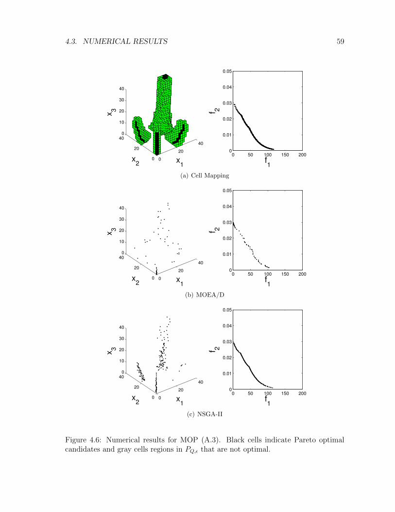
4.3. NUMERICAL RESULTS 59
0
20
40
0
20
40
0
10
20
30
40
x1
x2
x3
0 50 100 150 2000
0.01
0.02
0.03
0.04
0.05
f1
f 2
(a) Cell Mapping
0
20
40
0
20
40
0
10
20
30
40
x1
x2
x3
0 50 100 150 2000
0.01
0.02
0.03
0.04
0.05
f1
f 2
(b) MOEA/D
0
20
40
0
20
40
0
10
20
30
40
x1
x2
x3
0 50 100 150 2000
0.01
0.02
0.03
0.04
0.05
f1
f 2
(c) NSGA-II
Figure 4.6: Numerical results for MOP (A.3). Black cells indicate Pareto optimalcandidates and gray cells regions in PQ,ε that are not optimal.
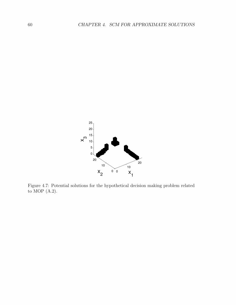
60 CHAPTER 4. SCM FOR APPROXIMATE SOLUTIONS
0
10
20
0
10
20
0
5
10
15
20
25
x1
x2
x3
Figure 4.7: Potential solutions for the hypothetical decision making problem relatedto MOP (A.2).
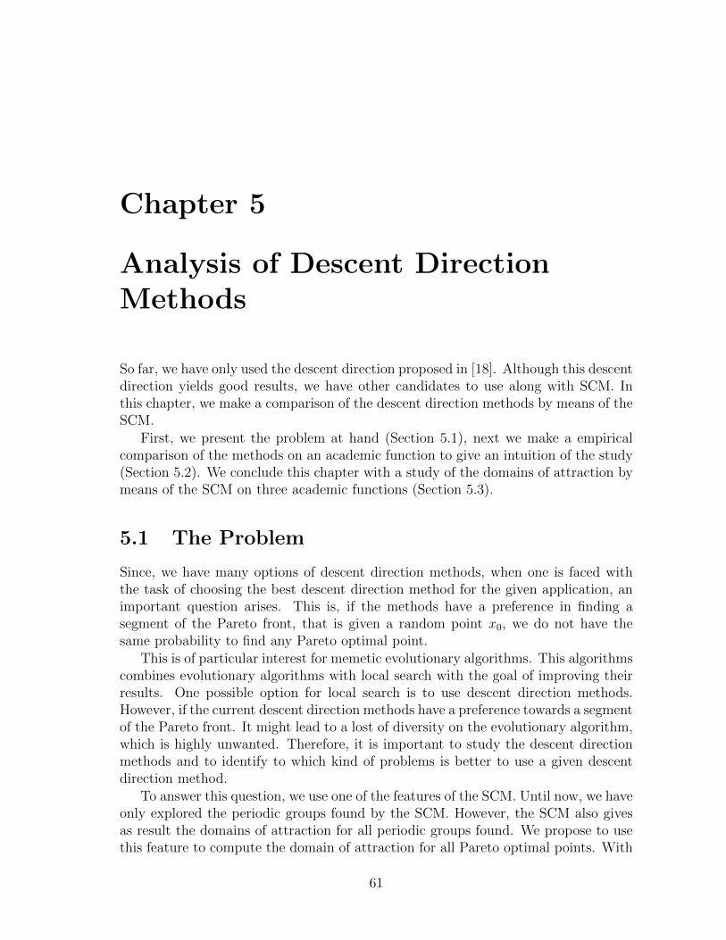
Chapter 5
Analysis of Descent DirectionMethods
So far, we have only used the descent direction proposed in [18]. Although this descentdirection yields good results, we have other candidates to use along with SCM. Inthis chapter, we make a comparison of the descent direction methods by means of theSCM.
First, we present the problem at hand (Section 5.1), next we make a empiricalcomparison of the methods on an academic function to give an intuition of the study(Section 5.2). We conclude this chapter with a study of the domains of attraction bymeans of the SCM on three academic functions (Section 5.3).
5.1 The Problem
Since, we have many options of descent direction methods, when one is faced withthe task of choosing the best descent direction method for the given application, animportant question arises. This is, if the methods have a preference in finding asegment of the Pareto front, that is given a random point x0, we do not have thesame probability to find any Pareto optimal point.
This is of particular interest for memetic evolutionary algorithms. This algorithmscombines evolutionary algorithms with local search with the goal of improving theirresults. One possible option for local search is to use descent direction methods.However, if the current descent direction methods have a preference towards a segmentof the Pareto front. It might lead to a lost of diversity on the evolutionary algorithm,which is highly unwanted. Therefore, it is important to study the descent directionmethods and to identify to which kind of problems is better to use a given descentdirection method.
To answer this question, we use one of the features of the SCM. Until now, we haveonly explored the periodic groups found by the SCM. However, the SCM also givesas result the domains of attraction for all periodic groups found. We propose to usethis feature to compute the domain of attraction for all Pareto optimal points. With
61
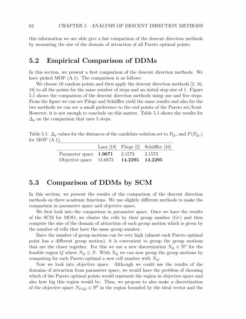
62 CHAPTER 5. ANALYSIS OF DESCENT DIRECTION METHODS
this information we are able give a fair comparison of the descent direction methodsby measuring the size of the domain of attraction of all Pareto optimal points.
5.2 Empirical Comparison of DDMs
In this section, we present a first comparison of the descent direction methods. Wehave picked MOP (A.1). The comparison is as follows:
We choose 10 random points and then apply the descent direction methods [2, 16,18] to all the points for the same number of steps and an initial step size of 1. Figure5.1 shows the comparison of the descent direction methods using one and five steps.From the figure we can see Fliege and Schaffler yield the same results and also for thetwo methods we can see a small preference to the end points of the Pareto set/front.However, it is not enough to conclude on this matter. Table 5.1 shows the results for∆p on the comparison that uses 5 steps.
Table 5.1: ∆p values for the distances of the candidate solution set to PQ,ε and F (PQ,ε)for MOP (A.1).
Lara [18] Fliege [2] Schaffler [16]
Parameter space 1.9671 2.1573 2.1573Objective space 15.6873 14.2295 14.2295
5.3 Comparison of DDMs by SCM
In this section, we present the results of the comparison of the descent directionmethods on three academic functions. We use slightly different methods to make thecomparison in parameter space and objective space.
We first look into the comparison in parameter space. Once we have the resultsof the SCM for MOO, we cluster the cells by their group number (Gr) and thencompute the size of the domain of attraction of each group motion which is given bythe number of cells that have the same group number.
Since the number of group motions can be very high (almost each Pareto optimalpoint has a different group motion), it is convenient to group the group motionsthat are the closer together. For this we use a new discretization NQ ∈ Nn for thefeasible region Q where NQ ≤ N . With NQ we can now group the group motions bycomputing for each Pareto optimal a new cell number with NQ.
Now we look into objective space. Although we could use the results of thedomains of attraction from parameter space, we would have the problem of choosingwhich of the Pareto optimal points would represent the region in objective space andalso how big this region would be. Thus, we propose to also make a discretizationof the objective space NF (Q) ∈ Nk in the region bounded by the ideal vector and the
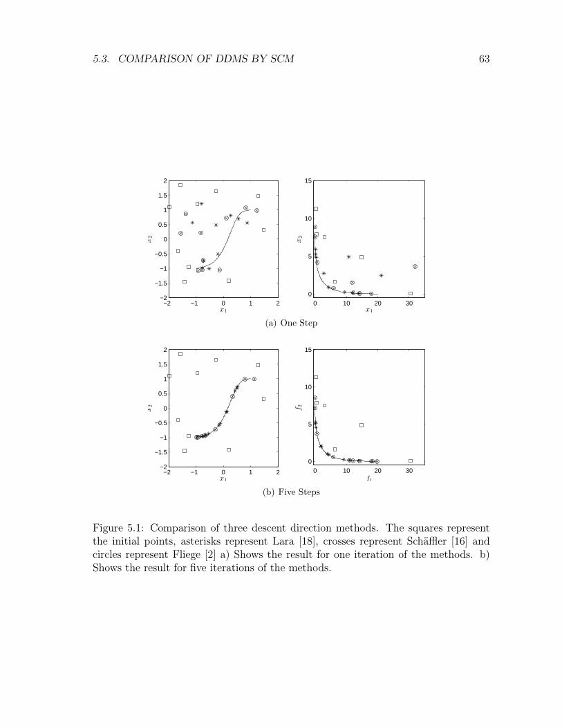
5.3. COMPARISON OF DDMS BY SCM 63
−2 −1 0 1 2−2
−1.5
−1
−0.5
0
0.5
1
1.5
2
x1
x2
0 10 20 300
5
10
15
x1
x2
(a) One Step
−2 −1 0 1 2−2
−1.5
−1
−0.5
0
0.5
1
1.5
2
x1
x2
0 10 20 300
5
10
15
f1
f2
(b) Five Steps
Figure 5.1: Comparison of three descent direction methods. The squares representthe initial points, asterisks represent Lara [18], crosses represent Schaffler [16] andcircles represent Fliege [2] a) Shows the result for one iteration of the methods. b)Shows the result for five iterations of the methods.

64 CHAPTER 5. ANALYSIS OF DESCENT DIRECTION METHODS
nadir vector. Then, we can group the groups motions in the same way as in parameterspace.
5.4 Numerical Results
In the following, we present the comparison for the descent direction methods. For allthe figures a lighter color means a bigger domain of attraction, while a darker colormeans a smaller domain of attraction.
5.4.1 Problem 1
First, we look into MOP (A.1). Figure 5.2 shows the result of SCM on cell spacewith a 10× 10 grid. Here we can see the mapping for the different descent directionsalong with the optimal solutions found. Figure 5.3 shows the result obtained by theSCM algorithm, the grid for SCM was set to N = [100, 100], NQ = [10, 10] andNF (Q) = [10, 10]. Apparently, all the methods show a preference towards the extremepoints of the both Pareto set and Pareto front. However, in Lara’s method is not asclear as it is for the other two methods.
5.4.2 Problem 2
Next, we look into MOP (A.4). Figure 5.4 shows the result of SCM on cell space with a21×21 grid. This allows to visually compare the difference on mapping for the descentdirection methods. Figure 5.5 shows the result obtained by the SCM algorithm, thegrid for SCM was set to N = [100, 100], NQ = [20, 20] and NF (Q) = [20, 20]. In thiscase, it is clearer a preference towards the extreme points of the sets.
5.4.3 Problem 3
Finally, we look into MOP (A.4). Figure 5.6 shows the result of SCM on cell spacewith a 21 × 21 grid. This allows to visually compare the difference on mapping forthe descent direction methods. Figure 5.7 shows the result obtained by the SCMalgorithm, the grid for SCM was set to N = [100, 100], NQ = [20, 20] and NF (Q) =[20, 20]. For Fliege and Schaffler it shows a preference for the optimal points in theleft and the size of the domain of attraction is smaller as we move to the right. We canalso notice that for this problem Fliege and Schaffler give different slightly differentresults, opposite to the previous problems where both were the same. In Lara we cansee a clear preference towards any section of the Pareto set/front.
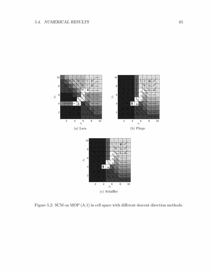
5.4. NUMERICAL RESULTS 65
2 4 6 8 10
2
4
6
8
10
N1
N2
(a) Lara
2 4 6 8 10
2
4
6
8
10
N1
N2
(b) Fliege
2 4 6 8 10
2
4
6
8
10
N1
N2
(c) Schaffler
Figure 5.2: SCM on MOP (A.1) in cell space with different descent direction methods.
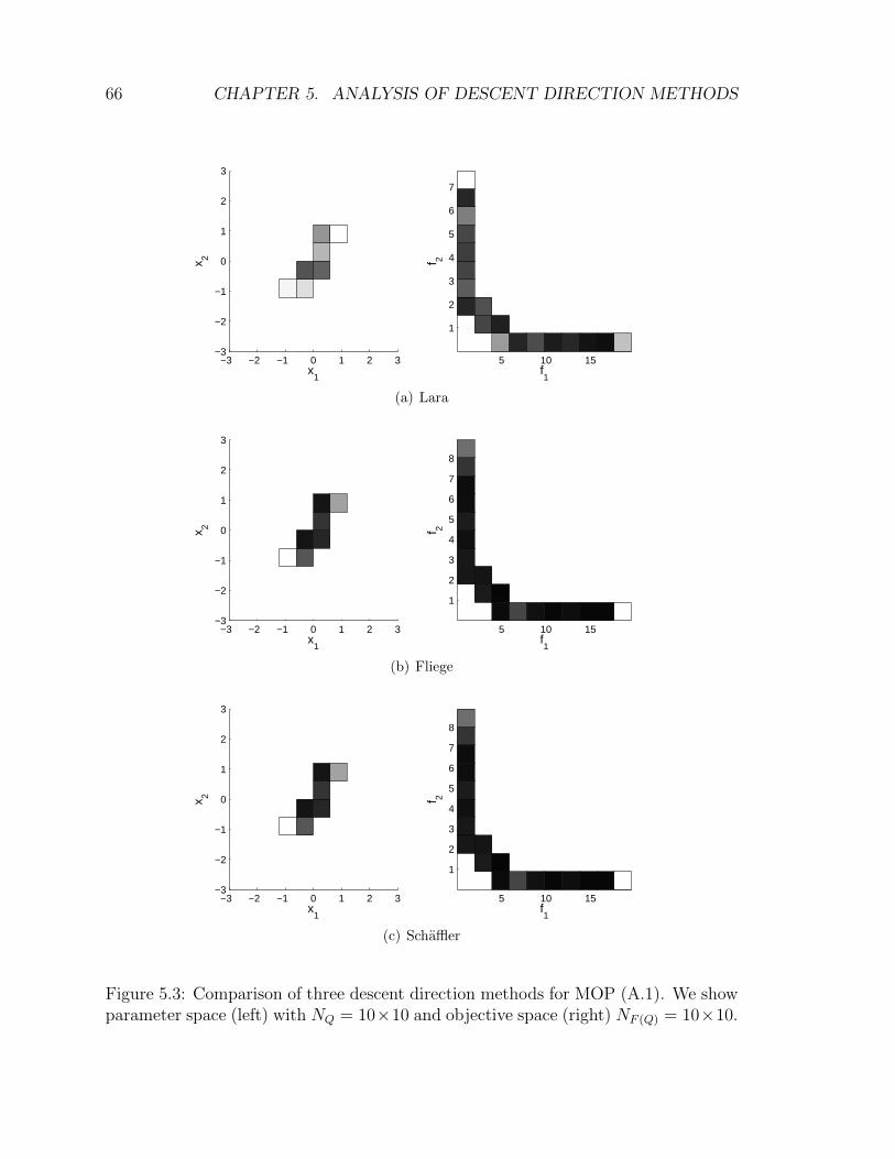
66 CHAPTER 5. ANALYSIS OF DESCENT DIRECTION METHODS
−3 −2 −1 0 1 2 3−3
−2
−1
0
1
2
3
x1
x 2
5 10 15
1
2
3
4
5
6
7
f1
f 2
(a) Lara
−3 −2 −1 0 1 2 3−3
−2
−1
0
1
2
3
x1
x 2
5 10 15
1
2
3
4
5
6
7
8
f1
f 2
(b) Fliege
−3 −2 −1 0 1 2 3−3
−2
−1
0
1
2
3
x1
x 2
5 10 15
1
2
3
4
5
6
7
8
f1
f 2
(c) Schaffler
Figure 5.3: Comparison of three descent direction methods for MOP (A.1). We showparameter space (left) with NQ = 10×10 and objective space (right) NF (Q) = 10×10.
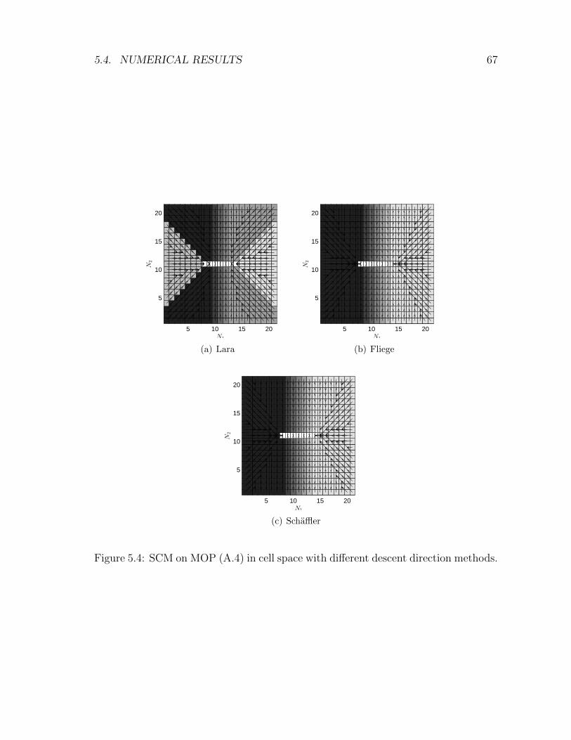
5.4. NUMERICAL RESULTS 67
5 10 15 20
5
10
15
20
N1
N2
(a) Lara
5 10 15 20
5
10
15
20
N1
N2
(b) Fliege
5 10 15 20
5
10
15
20
N1
N2
(c) Schaffler
Figure 5.4: SCM on MOP (A.4) in cell space with different descent direction methods.
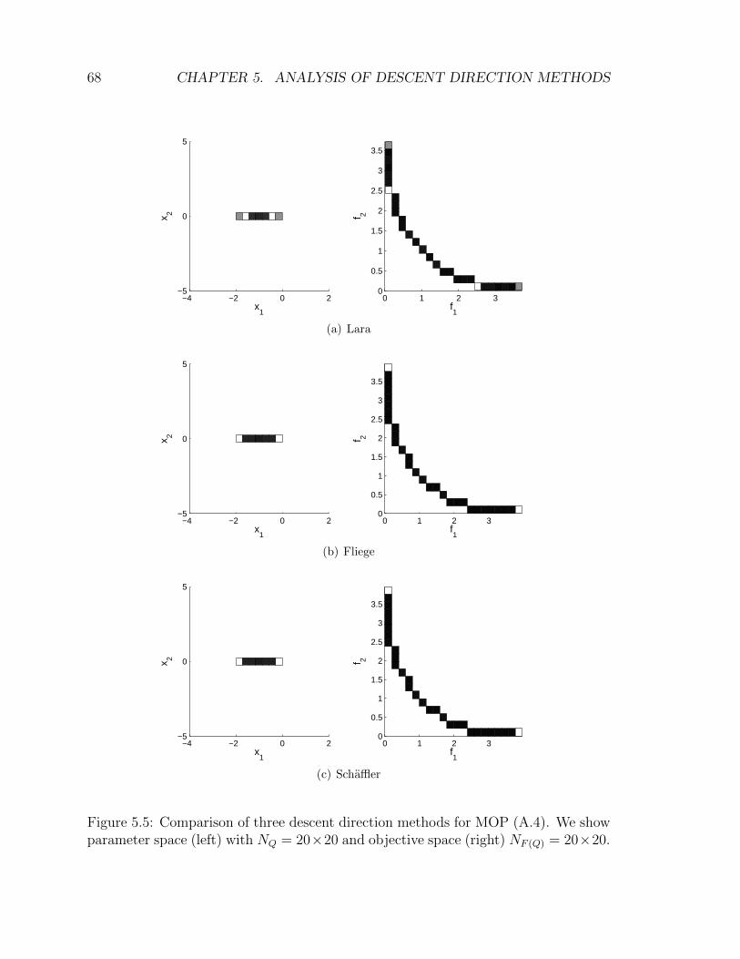
68 CHAPTER 5. ANALYSIS OF DESCENT DIRECTION METHODS
−4 −2 0 2−5
0
5
x1
x 2
0 1 2 30
0.5
1
1.5
2
2.5
3
3.5
f1
f 2
(a) Lara
−4 −2 0 2−5
0
5
x1
x 2
0 1 2 30
0.5
1
1.5
2
2.5
3
3.5
f1
f 2
(b) Fliege
−4 −2 0 2−5
0
5
x1
x 2
0 1 2 30
0.5
1
1.5
2
2.5
3
3.5
f1
f 2
(c) Schaffler
Figure 5.5: Comparison of three descent direction methods for MOP (A.4). We showparameter space (left) with NQ = 20×20 and objective space (right) NF (Q) = 20×20.
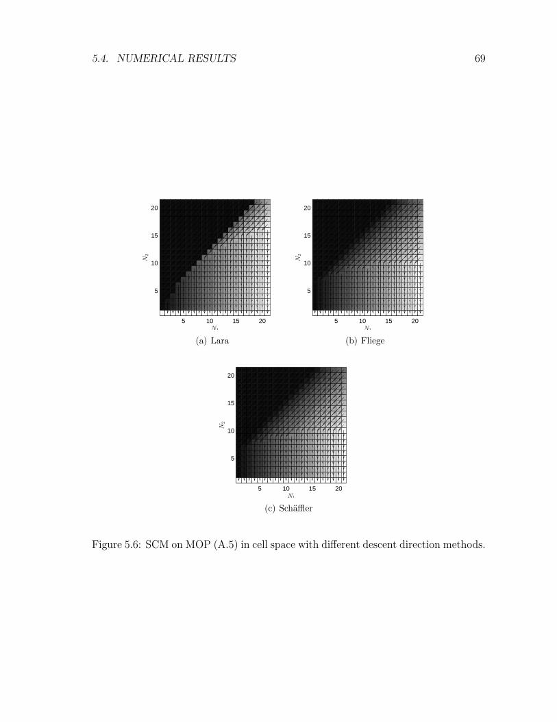
5.4. NUMERICAL RESULTS 69
5 10 15 20
5
10
15
20
N1
N2
(a) Lara
5 10 15 20
5
10
15
20
N1
N2
(b) Fliege
5 10 15 20
5
10
15
20
N1
N2
(c) Schaffler
Figure 5.6: SCM on MOP (A.5) in cell space with different descent direction methods.
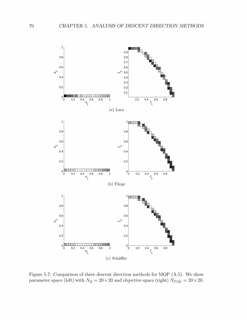
70 CHAPTER 5. ANALYSIS OF DESCENT DIRECTION METHODS
0 0.2 0.4 0.6 0.8 10
0.2
0.4
0.6
0.8
1
x1
x 2
0.2 0.4 0.6 0.8
0.1
0.2
0.3
0.4
0.5
0.6
0.7
0.8
0.9
f1
f 2
(a) Lara
0 0.2 0.4 0.6 0.8 10
0.2
0.4
0.6
0.8
1
x1
x 2
0 0.2 0.4 0.6 0.80
0.2
0.4
0.6
0.8
1
f1
f 2
(b) Fliege
0 0.2 0.4 0.6 0.8 10
0.2
0.4
0.6
0.8
1
x1
x 2
0 0.2 0.4 0.6 0.80
0.2
0.4
0.6
0.8
1
f1
f 2
(c) Schaffler
Figure 5.7: Comparison of three descent direction methods for MOP (A.5). We showparameter space (left) with NQ = 20×20 and objective space (right) NF (Q) = 20×20.
Chapter 6
Refine and Recover
One of the potential drawbacks of the SCM is given by the size of the cells. Thechoice of the size of the cells is critical for the algorithm, since cells too small maylead to a high number of function evaluations, while cells too big may lead to resultsthat are not significant enough or even in the lost of information.
In this chapter, we address the problem of refining the solutions once the SCMhas computed the optimal solutions (Section 6.1) and then we address the problemof how to recover optimal solutions once they have been discarded by the SCM duethe discretization of the feasible region Q (Section 6.2).
6.1 Refine
Although there is a risk on using a big size of cell, the SCM can be used to computea raw picture of promissory regions where optimal solutions can be found. Withthis preliminary result, now we can focus in these regions to perform a fine search.In this section, we present several methods that can be used in this context. First,we present a method that given the center points of each cell that belongs to anoptimal solution, it searches for the best point within its cell (Section 6.1.1). Next,we present a variation of the SCM method that takes a subspace of the feasibleregion Q and then performs the SCM (Section 6.1.2). Further, we examine in howto use the subdivision techniques together with the SCM (Section 6.1.3). Finally, wepresent a comparison between the methods proposed in this section and the SCM formulti-objective optimization (Section 6.1.4).
6.1.1 Refine in Cell
As we mentioned previously the center point method has the disadvantage that thecenter point may not be significant of the whole cell. When a cell is marked asan optimal solution, it means that within the cell, we can find an optimal solution.However in the SCM, we always take the center point to represent the cell, thus itcan be the case that there are better solutions rather than the center point.
71
72 CHAPTER 6. REFINE AND RECOVER
The idea of this method is the following: Given the center point xc of a cell and itsboundaries lbcell and ubcell, we use the dynamical systems with lbcell and ubcell as boxconstraints and we use xc as initial point. Thus, we will find a new point xc+j afterj steps such that xc+j ≺ xc. Algorithm 8 shows the key elements of this approachcalled rinc.
Algorithm 8 Refine in Cell (rinc)
Require: DynamicalSystem, cPs,maxiter, toleranceEnsure: refined solution
1: refined solution← {}2: for all cell ∈ cPs do3: i← 14: xc ← compute center of cell with Equation (3.1)5: lbcell, ubcell ← compute lower and upper bounds of cell6: while i ≤ maxiter and stopcriteria(xc) > tolerance do7: xc ← DynamicalSystem(xc)8: end while9: refined solution← refined solution ∪ {xc}
10: end for
This method has the property that it will output the same number of solutionsas the input had. However, it has two potential drawbacks. First, although severaloptimal solutions may exist in the same cell but the method only give one for eachcell. Further, due the step size control, periodic groups bigger than one may appear.Thus a cell marked as optimal solution may not in fact be one, in this case the methodis not capable of detecting it and will give as output a point in the boundary of a cell.
6.1.2 SCM-Refine
As we can see in Algorithm 2, the SCM takes as input a feasible region boundedby box constraints lb and ub. We propose to give as input a set of feasible cellscelli such that i ∈ n and everything outside this set is considered to be the sink cell.This idea allows the SCM to skip cells that are not interesting by a given criteria, i.e.the cell is not feasible.
Thus, once we have the result of the SCM using only box constraints, we can selectthe cells that are optimal solutions. Next, we divide these cells by a given factor c andthen use the SCM only with these cells and compute a new set of optimal solutions.Algorithm 9 shows the key elements of this method (SCM-R).
This method has the advantages that we are able to compute more than oneoptimal solution for each cell. Also the method can be used several times until itmeets a criteria. For instance, on the size of the cells or the number of solutions.Finally, this method compute not only the new set of optimal solutions but also thedomains of attraction of the new set, which can be both an advantage of a drawback,if we are interested or not in the domains of attraction.
6.1. REFINE 73
Algorithm 9 SCM-Refine
Require: DynamicalSystem, cPs, div, h,NEnsure: cPs
1: S ← {}2: hi ← hi/divi3: Ni ← Ni ∗ divi4: rangi ← −divi + 1,−div, . . . , 0, i = 1, . . . , |div|5: comb← rang1 × . . .× rang|div|6: for all cell ∈ cPs do7: z ← compute cell coordinates of cell with Algorithm (3)8: corneri ← zidivi, i = 1, . . . , |div|9: new cells← combi + corner, i = 1, . . . , |div|
10: end for11: S ← S ∪ new cells12: z, C,Gr, Pe, St, cPs← SCM(DynamicalSystem, F, ub, lb, N, h,Nc, S)
6.1.3 SCM with subdivision techniques
The subdivision techniques are an effective way to compute the optimal solutions ofa given MOP and the subdivision techniques has also been proved to converge to theoptimal solutions [40]. However, in the realization of the algorithm, when the cellsare too big (for instance in the initial iterations), it is more difficult to decide if agiven cell fulfills the selection criteria. In this section, we propose to use the SCM(SCM-ST) to preprocess the feasible region Q.
Again, we select the optimal solutions given by the SCM. Next, we convert thecells to a (center, radius) representation. Finally, we use the new set of cells as initialparameter for the subdivision techniques.
This method has also the advantage of computing more than one optimal solutionfor each original cell. Also, if we are not interested in the domains of attraction ofthe new set of optimal solutions, this method only computes the optimal solutions.Thus, it is cheaper in terms of memory than the previous method, since we do notcompute the global properties of the dynamical system.
6.1.4 Comparison of the methods
In this section, we present a numerical comparison of the refinement methods pre-sented above for MOP (A.1). A budget of 10, 000 function evaluations was used asin Section 3.4. First a result with SCM was computed. The grid for rinc was set toN = [35, 35] (7350 function evaluations) leading to 21 optimal solutions and for theother cases was set to N = [20, 20] (2400 function evaluations) leading to 11 optimalsolutions.
Next, for rinc 17 steps of the dynamical system were used for each optimal solutionfound. In the case of both SCM-ST and SCM-R a division factor of 2 was used and
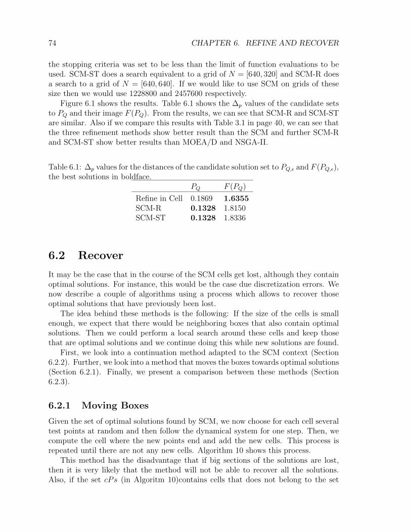
74 CHAPTER 6. REFINE AND RECOVER
the stopping criteria was set to be less than the limit of function evaluations to beused. SCM-ST does a search equivalent to a grid of N = [640, 320] and SCM-R doesa search to a grid of N = [640, 640]. If we would like to use SCM on grids of thesesize then we would use 1228800 and 2457600 respectively.
Figure 6.1 shows the results. Table 6.1 shows the ∆p values of the candidate setsto PQ and their image F (PQ). From the results, we can see that SCM-R and SCM-STare similar. Also if we compare this results with Table 3.1 in page 40, we can see thatthe three refinement methods show better result than the SCM and further SCM-Rand SCM-ST show better results than MOEA/D and NSGA-II.
Table 6.1: ∆p values for the distances of the candidate solution set to PQ,ε and F (PQ,ε),the best solutions in boldface.
PQ F (PQ)
Refine in Cell 0.1869 1.6355SCM-R 0.1328 1.8150SCM-ST 0.1328 1.8336
6.2 Recover
It may be the case that in the course of the SCM cells get lost, although they containoptimal solutions. For instance, this would be the case due discretization errors. Wenow describe a couple of algorithms using a process which allows to recover thoseoptimal solutions that have previously been lost.
The idea behind these methods is the following: If the size of the cells is smallenough, we expect that there would be neighboring boxes that also contain optimalsolutions. Then we could perform a local search around these cells and keep thosethat are optimal solutions and we continue doing this while new solutions are found.
First, we look into a continuation method adapted to the SCM context (Section6.2.2). Further, we look into a method that moves the boxes towards optimal solutions(Section 6.2.1). Finally, we present a comparison between these methods (Section6.2.3).
6.2.1 Moving Boxes
Given the set of optimal solutions found by SCM, we now choose for each cell severaltest points at random and then follow the dynamical system for one step. Then, wecompute the cell where the new points end and add the new cells. This process isrepeated until there are not any new cells. Algorithm 10 shows this process.
This method has the disadvantage that if big sections of the solutions are lost,then it is very likely that the method will not be able to recover all the solutions.Also, if the set cPs (in Algoritm 10)contains cells that does not belong to the set

6.2. RECOVER 75
−2 −1 0 1 2−2
−1.5
−1
−0.5
0
0.5
1
1.5
2
x1
x2
0 5 10 15 200
5
10
15
20
f1
f2
(a) Refine in Cell
−2 −1 0 1 2−2
−1.5
−1
−0.5
0
0.5
1
1.5
2
x1
x2
0 5 10 15 200
5
10
15
20
f1
f2
(b) SCM-Refine
−2 −1 0 1 2−2
−1.5
−1
−0.5
0
0.5
1
1.5
2
x1
x2
0 5 10 15 200
5
10
15
20
f1
f2
(c) SCM with Subdivision Techniques
Figure 6.1: Numerical results for MOP (A.1). Black cells indicate Pareto optimalcandidates.
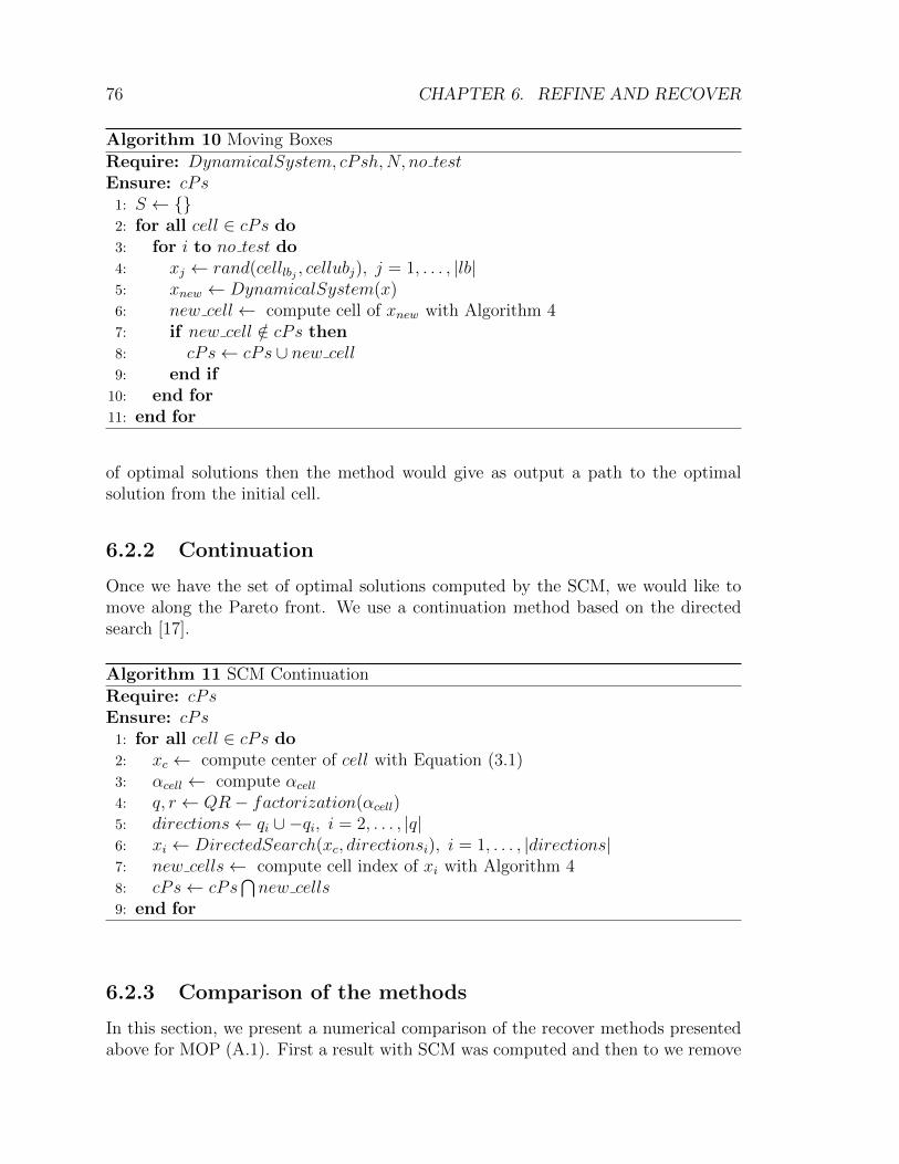
76 CHAPTER 6. REFINE AND RECOVER
Algorithm 10 Moving Boxes
Require: DynamicalSystem, cPsh,N, no testEnsure: cPs
1: S ← {}2: for all cell ∈ cPs do3: for i to no test do4: xj ← rand(celllbj , cellubj), j = 1, . . . , |lb|5: xnew ← DynamicalSystem(x)6: new cell← compute cell of xnew with Algorithm 47: if new cell /∈ cPs then8: cPs← cPs ∪ new cell9: end if
10: end for11: end for
of optimal solutions then the method would give as output a path to the optimalsolution from the initial cell.
6.2.2 Continuation
Once we have the set of optimal solutions computed by the SCM, we would like tomove along the Pareto front. We use a continuation method based on the directedsearch [17].
Algorithm 11 SCM Continuation
Require: cPsEnsure: cPs
1: for all cell ∈ cPs do2: xc ← compute center of cell with Equation (3.1)3: αcell ← compute αcell4: q, r ← QR− factorization(αcell)5: directions← qi ∪ −qi, i = 2, . . . , |q|6: xi ← DirectedSearch(xc, directionsi), i = 1, . . . , |directions|7: new cells← compute cell index of xi with Algorithm 48: cPs← cPs
⋂new cells
9: end for
6.2.3 Comparison of the methods
In this section, we present a numerical comparison of the recover methods presentedabove for MOP (A.1). First a result with SCM was computed and then to we remove
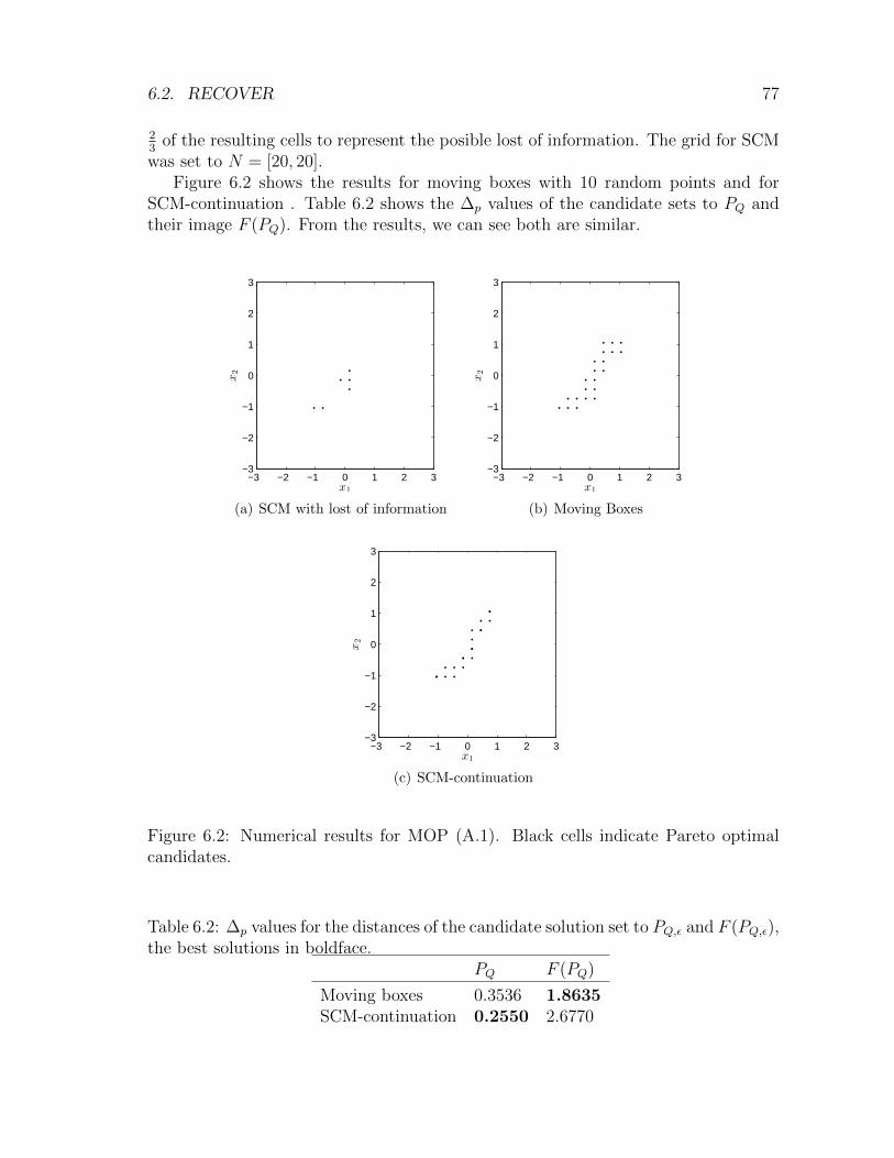
6.2. RECOVER 77
23
of the resulting cells to represent the posible lost of information. The grid for SCMwas set to N = [20, 20].
Figure 6.2 shows the results for moving boxes with 10 random points and forSCM-continuation . Table 6.2 shows the ∆p values of the candidate sets to PQ andtheir image F (PQ). From the results, we can see both are similar.
−3 −2 −1 0 1 2 3−3
−2
−1
0
1
2
3
x1
x2
(a) SCM with lost of information
−3 −2 −1 0 1 2 3−3
−2
−1
0
1
2
3
x1
x2
(b) Moving Boxes
−3 −2 −1 0 1 2 3−3
−2
−1
0
1
2
3
x1
x2
(c) SCM-continuation
Figure 6.2: Numerical results for MOP (A.1). Black cells indicate Pareto optimalcandidates.
Table 6.2: ∆p values for the distances of the candidate solution set to PQ,ε and F (PQ,ε),the best solutions in boldface.
PQ F (PQ)
Moving boxes 0.3536 1.8635SCM-continuation 0.2550 2.6770

78 CHAPTER 6. REFINE AND RECOVER
Chapter 7
Conclusions and Future Work
7.1 Conclusions
The main goal of this thesis has been to design set oriented methods for the numericaltreatment of multi-objective optimization problems. The proposed approach was toadapt the simple cell mapping method to the given context. With this approach weobtained a thorough investigation for low dimensional problems.
We have used the simple cell mapping techniques to address the problem of com-puting the set of approximate solutions of a given multi-objective optimization prob-lem. This set is of interest for the decision maker since it might enhance the set ofoptions for him/her when compared to the set of optimal solutions, the Pareto set. Tocompute the set of approximate solutions we have adapted cell mapping techniquesthat were originally designed for the global analysis of dynamical systems. Sincemethods of that kind divide the search space into n-dimensional cells, where n is thedimension of the decision space of the MOP, they are well-suited for the problem athand since they allow for an efficient approximation of the set of interest. We havetested the novel method on three academic functions and have compared it againsttwo evolutionary methods. The results indicate that the cell mapping technique isable to reliably compute the set of approximate solutions, and is faster than theevolutionary approaches.
Further, we have made a comparison of some of the existing descent directionmethods. This comparison is of particular interest for memetic evolutionary algo-rithms, since the results indicate that the studied methods have a potential biastowards the extreme points of the Pareto front. This should be taken to accountwhen designing a memetic evolutionary algorithm based on this methods, since it canlead to unwanted issues as a lost on diversity.
Finally, we have also hybridized the simple cell mapping method with other tech-niques to partially overcome some of the drawbacks of the method. In particularwe have addressed the refinement of the solutions once a prominent region has beenfound and the potential lost of information due discretization errors. The resultsshow that this approach is highly competitive with the evolutionary algorithms for
79
80 CHAPTER 7. CONCLUSIONS AND FUTURE WORK
low dimension problems.
7.2 Future Work
There are several points to be addressed. First of all, it would be desirable to extendthe applicability of the method to higher dimensional problems. For this it seemspromising to parallelize the simple cell mapping method.
Next, the integration of constraint handling techniques has to be addresses whichhas been left out in this study.
It would also be interesting to extend the refinement and recovering techniques tothe other sets of interest such as approximate solutions and domains of attractions.
For our study, we have used academic models. However, we plan to apply the newmethod to real-wold engineering problems.
In the case of the comparison of descent direction methods, it would be desirableto improve it and to design a framework to help us study these methods and also toeither improve them or to design a bias free descent direction method.
Finally, we plan to use the simple cell mapping to address robust multi-objectiveoptimization, since it seems to be a good candidate given the thorough investigationprovided by simple cell mapping.
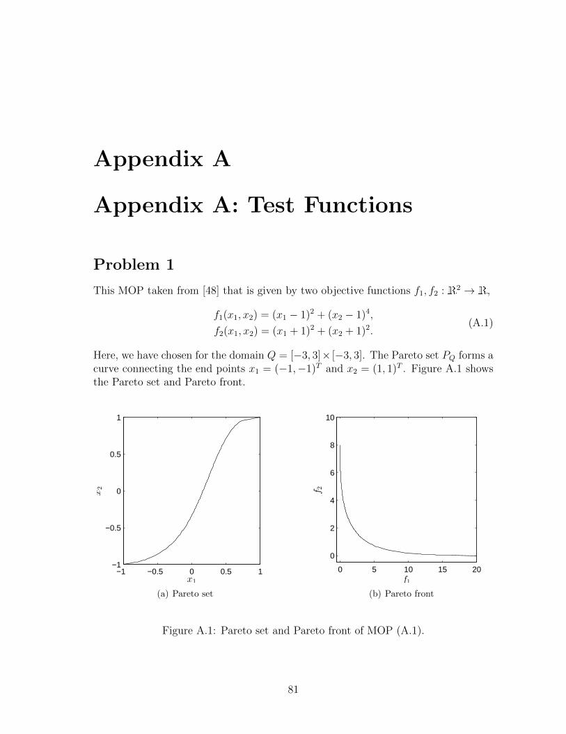
Appendix A
Appendix A: Test Functions
Problem 1
This MOP taken from [48] that is given by two objective functions f1, f2 : R2 → R,
f1(x1, x2) = (x1 − 1)2 + (x2 − 1)4,
f2(x1, x2) = (x1 + 1)2 + (x2 + 1)2.(A.1)
Here, we have chosen for the domain Q = [−3, 3]× [−3, 3]. The Pareto set PQ forms acurve connecting the end points x1 = (−1,−1)T and x2 = (1, 1)T . Figure A.1 showsthe Pareto set and Pareto front.
−1 −0.5 0 0.5 1−1
−0.5
0
0.5
1
x1
x2
(a) Pareto set
0 5 10 15 20
0
2
4
6
8
10
f1
f2
(b) Pareto front
Figure A.1: Pareto set and Pareto front of MOP (A.1).
81
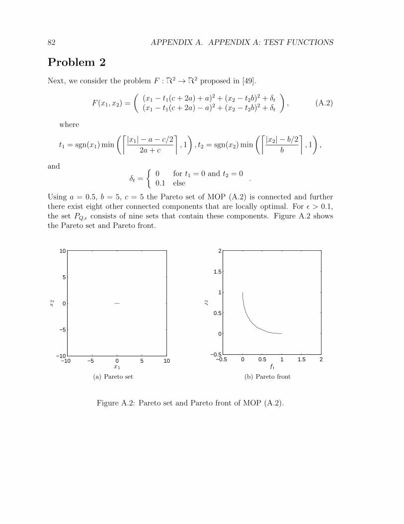
82 APPENDIX A. APPENDIX A: TEST FUNCTIONS
Problem 2
Next, we consider the problem F : R2 → R2 proposed in [49].
F (x1, x2) =
((x1 − t1(c+ 2a) + a)2 + (x2 − t2b)2 + δt(x1 − t1(c+ 2a)− a)2 + (x2 − t2b)2 + δt
), (A.2)
where
t1 = sgn(x1) min
(⌈|x1| − a− c/2
2a+ c
⌉, 1
), t2 = sgn(x2) min
(⌈|x2| − b/2
b
⌉, 1
),
and
δt =
{0 for t1 = 0 and t2 = 00.1 else
.
Using a = 0.5, b = 5, c = 5 the Pareto set of MOP (A.2) is connected and furtherthere exist eight other connected components that are locally optimal. For ε > 0.1,the set PQ,ε consists of nine sets that contain these components. Figure A.2 showsthe Pareto set and Pareto front.
−10 −5 0 5 10−10
−5
0
5
10
x1
x2
(a) Pareto set
−0.5 0 0.5 1 1.5 2−0.5
0
0.5
1
1.5
2
f1
f2
(b) Pareto front
Figure A.2: Pareto set and Pareto front of MOP (A.2).
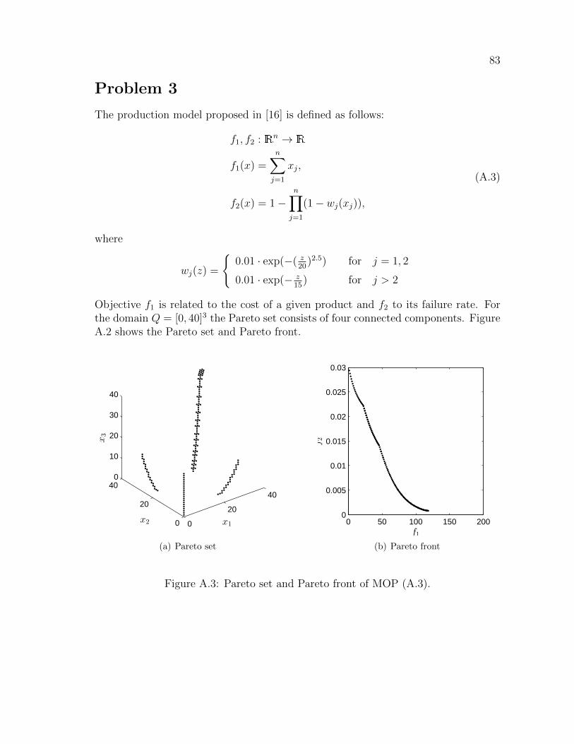
83
Problem 3
The production model proposed in [16] is defined as follows:
f1, f2 : Rn → R
f1(x) =n∑j=1
xj,
f2(x) = 1−n∏j=1
(1− wj(xj)),
(A.3)
where
wj(z) =
{0.01 · exp(−( z
20)2.5) for j = 1, 2
0.01 · exp(− z15
) for j > 2
Objective f1 is related to the cost of a given product and f2 to its failure rate. Forthe domain Q = [0, 40]3 the Pareto set consists of four connected components. FigureA.2 shows the Pareto set and Pareto front.
0
20
40
0
20
400
10
20
30
40
x1x2
x3
(a) Pareto set
0 50 100 150 2000
0.005
0.01
0.015
0.02
0.025
0.03
f1
f2
(b) Pareto front
Figure A.3: Pareto set and Pareto front of MOP (A.3).
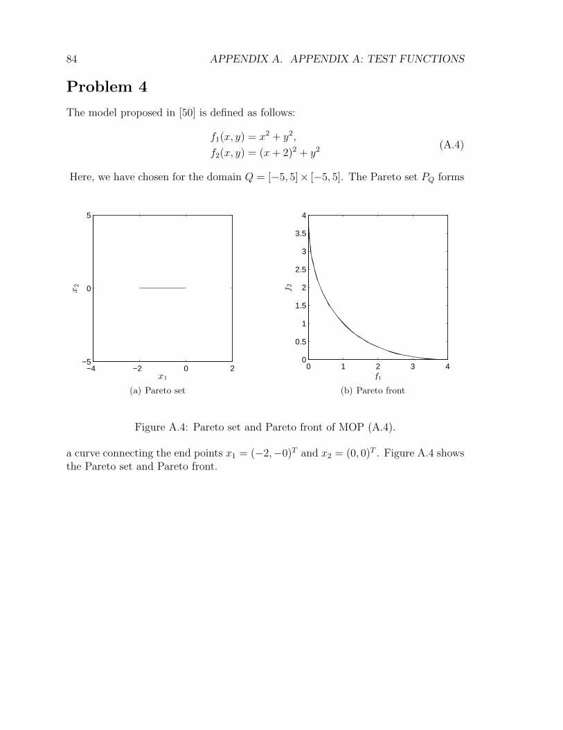
84 APPENDIX A. APPENDIX A: TEST FUNCTIONS
Problem 4
The model proposed in [50] is defined as follows:
f1(x, y) = x2 + y2,
f2(x, y) = (x+ 2)2 + y2(A.4)
Here, we have chosen for the domain Q = [−5, 5]× [−5, 5]. The Pareto set PQ forms
−4 −2 0 2−5
0
5
x1
x2
(a) Pareto set
0 1 2 3 40
0.5
1
1.5
2
2.5
3
3.5
4
f1
f2
(b) Pareto front
Figure A.4: Pareto set and Pareto front of MOP (A.4).
a curve connecting the end points x1 = (−2,−0)T and x2 = (0, 0)T . Figure A.4 showsthe Pareto set and Pareto front.
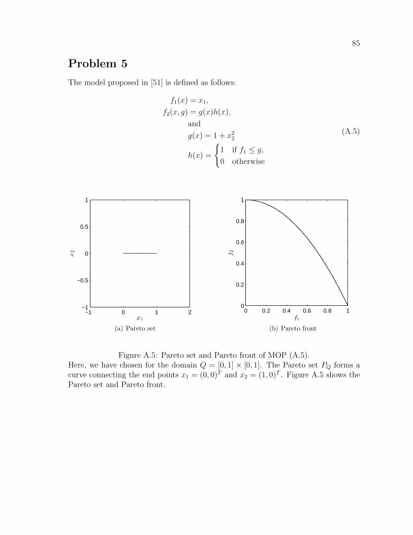
85
Problem 5
The model proposed in [51] is defined as follows:
f1(x) = x1,
f2(x, g) = g(x)h(x),
and
g(x) = 1 + x22
h(x) =
{1 if f1 ≤ g,
0 otherwise
(A.5)
−1 0 1 2−1
−0.5
0
0.5
1
x1
x2
(a) Pareto set
0 0.2 0.4 0.6 0.8 10
0.2
0.4
0.6
0.8
1
f1
f2
(b) Pareto front
Figure A.5: Pareto set and Pareto front of MOP (A.5).Here, we have chosen for the domain Q = [0, 1] × [0, 1]. The Pareto set PQ forms acurve connecting the end points x1 = (0, 0)T and x2 = (1, 0)T . Figure A.5 shows thePareto set and Pareto front.
86 APPENDIX A. APPENDIX A: TEST FUNCTIONS
Problem PID
We consider a second order oscillator subject to a proportional-integral-derivative(PID) control [52].
x+ 2ζωnx+ ω2nx = ω2
nu(t), (A.6)
where ωn = 5, ζ = 0.01,
u(t) = kp [r(t)− x(t)] + ki
∫ t
0
[r(t)− x(t)
]dt− kdx(t), (A.7)
r(t) is a step input, kp, ki and kd are the PID control gains. We consider the MOP
with the control gains k = [kp, ki, kd]T as design parameters. The design space for the
parameters is chosen as follows,
Q = {k ∈ [10, 50]× [1, 30]× [1, 2] ⊂ R3}. (A.8)
Peak time and overshoot are common in time domain control design objectives[53, 54, 55]. We consider the multi-objective optimization problem to design thecontrol gain k,
mink∈Q{tp,Mp, eIAE}, (A.9)
where Mp stands for the overshoot of the response to a step reference input, tp is thecorresponding peak time and eIAE is the integrated absolute tracking error
eIAE =
∫ Tss
0
∣∣r(t)− x(t)∣∣ dt. (A.10)
Where r(t) is a reference input and Tss is the time when the response is close to bein the steady state. The closed-loop response of the system for each design trial iscomputed with the help of closed form solutions. The integrated absolute trackingerror eIAE is calculated over time with Tss = 20s.
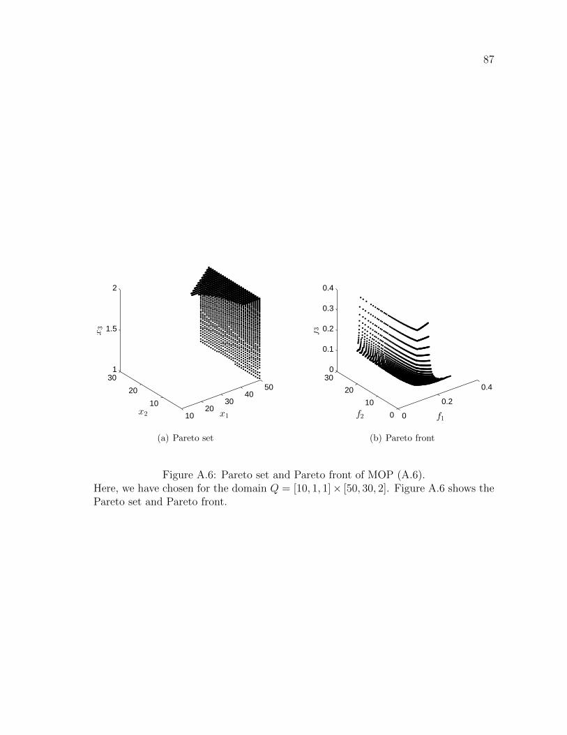
87
1020
3040
50
10
20
301
1.5
2
x1x2
x3
(a) Pareto set
0
0.2
0.4
0
10
20
300
0.1
0.2
0.3
0.4
f1f2
f3
(b) Pareto front
Figure A.6: Pareto set and Pareto front of MOP (A.6).Here, we have chosen for the domain Q = [10, 1, 1]× [50, 30, 2]. Figure A.6 shows thePareto set and Pareto front.

88 APPENDIX A. APPENDIX A: TEST FUNCTIONS
Bibliography
[1] I. Das and J. Dennis. Normal-boundary intersection: A new method for gener-ating the Pareto surface in nonlinear multicriteria optimization problems. SIAMJournal of Optimization, 8:631–657, 1998.
[2] J. Fliege and B. F. Svaiter. Steepest Descent Methods for Multicriteria Opti-mization. Mathematical Methods of Operations Research, 51(3):479–494, 2000.
[3] K. Klamroth and J. Tind and M. Wiecek. Unbiased Approximation in Multicri-teria Optimization. Mathematical Methods of Operations Research, 56:413–437,2002.
[4] J. Fliege. Gap-free computation of Pareto-points by quadratic scalarizations.Mathematical Methods of Operations Research, 59:69–89, 2004.
[5] E.L. Allgower and K. Georg. Numerical Continuation Methods. Springer, 1990.
[6] C. Hillermeier. Nonlinear Multiobjective Optimization - A Generalized HomotopyApproach. Birkhauser, 2001.
[7] O. Schutze and A. Dell’Aere and M. Dellnitz. On Continuation Meth-ods for the Numerical Treatment of Multi-Objective Optimization Prob-lems. In Jurgen Branke and Kalyanmoy Deb and Kaisa Miettinen andRalph E. Steuer, editor, Practical Approaches to Multi-Objective Opti-mization, number 04461 in Dagstuhl Seminar Proceedings. InternationalesBegegnungs- und Forschungszentrum (IBFI), Schloss Dagstuhl, Germany, 2005.<http://drops.dagstuhl.de/opus/volltexte/2005/349>.
[8] V. Pereyra. Fast computation of equispaced Pareto manifolds and Pareto frontsfor multiobjective optimization problems. Math. Comput. Simul., 79(6):1935–1947, 2009.
[9] M. Dellnitz and O. Schutze and T. Hestermeyer. Covering Pareto Sets by Multi-level Subdivision Techniques. Journal of Optimization Theory and Applications,124:113–155, 2005.
[10] J. Jahn. Multiobjective search algorithm with subdivision technique. Computa-tional Optimization and Applications, 35(2):161–175, 2006.
89

90 BIBLIOGRAPHY
[11] O. Schutze and M. Vasile and O. Junge and M. Dellnitz and D. Izzo. Designingoptimal low thrust gravity assist trajectories using space pruning and a multi-objective approach. Engineering Optimization, 41(2):155–181, 2009.
[12] K. Deb. Optimization using Evolutionary Algorithms. John Wiley & Sons, 2001.
[13] C. Coello Coello and G. Lamont and D. Van Veldhuizen. Evolutionary Algorithmsfor Solving Multi-Objective Problems. Springer, Second edition, 2007.
[14] O. Schutze and M. Laumanns and C. A. Coello Coello and M. Dellnitz and E.-G.Talbi. Convergence of Stochastic Search Algorithms to Finite Size Pareto SetApproximations. Journal of Global Optimization, 41(4):559–577, 2008.
[15] C.S. Hsu. Cell-to-cell mapping: A method of global analysis for nonlinear sys-tems. Applied mathematical sciences. Springer-Verlag, 1987.
[16] S. Schaffler and R. Schultz and K. Weinzierl. A stochastic method for the solutionof unconstrained vector opimization problems. Journal of Optimization, Theoryand Application, 114(1):209–222, 2002.
[17] O. Schutze and A. Lara and C. A. Coello. The Directed Search Method forUnconstrained Multi-Objective Optimization Problems. Technical Report COA-R1, CINVESTAV-IPN, 2010.
[18] A. Lara Lopez. Using Gradient Based Information to build Hybrid Multi-objectiveEvolutionary Algorithms. PhD thesis, 2012.
[19] V. Pareto. Manual of Political Economy. The MacMillan Press, 1971 (originaledition in French in 1927).
[20] K. M. Miettinen. Nonlinear Multiobjective Optimization. Kluwer Academic Pub-lishers, 1999.
[21] P. Loridan. ε-Solutions in Vector Minimization Problems. Journal of Optimiza-tion, Theory and Application, 42:265–276, 1984.
[22] O. Schutze and C. A. Coello Coello and E.-G. Talbi. Approximating the ε-efficientset of an MOP with stochastic search algorithms. In A. Gelbukh and A. F.Kuri Morales, editor, Mexican International Conference on Artificial Intelligence(MICAI-2007), pages 128–138. Springer-Verlag Berlin Heidelberg, 2007.
[23] H. Kuhn and A. Tucker. Nonlinear programming. Proc. Berkeley Symp. MathStatist. Probability, page 481–492, 1951.
[24] Y.Y. Haimes and L.S. Lasdon and D.A. Wismer. On bicriterion formulation ofthe problems of integrated system identification and system optimization. IEEETransactions on Systems, Man, and Cybernetics, 1(3):296–297, 1971.
BIBLIOGRAPHY 91
[25] N. Srinivas and K. Deb. Multiobjective function optimization using nondomi-nated sorting genetic algorithms. Evolutionary Computation Journal, 2:221–248,1995.
[26] Q. Zhang and H. Li. MOEA/D: A Multi-objective Evolutionary AlgorithmBased on Decomposition. IEEE Trans. on Evolutionary Computation, 11:712–731, 2007.
[27] O. Schutze, M. Vasile, and C. A. Coello Coello. Approximate solutions in spacemission design. In Proceedings of the 10th International Conference on ParallelProblem Solving From Nature, page 805–814, 2008.
[28] E. Zitzler and L. Thiele and M. Laumanns and C. M. Fonseca and V.Fonseca.Performance Assessment of Multiobjective Optimizers: An Analysis and Review.IEEE Transactions on Evolutionary Computation, 7(2):117–132, 2003.
[29] D. A. Van Veldhuizen. Multiobjective Evolutionary Algorithms: Classifications,Analyses, and New Innovations. PhD thesis, Department of Electrical and Com-puter Engineering. Graduate School of Engineering. Air Force Institute of Tech-nology, Wright-Patterson AFB, Ohio, May 1999.
[30] O. Schutze and X. Esquivel and A. Lara and C. A. Coello Coello. Usingthe averaged Hausdorff distance as a performance measure in evolutionarymulti-objective optimization. IEEE Transactions on Evolutionary Computation,16(4):504–522, 2012.
[31] C. A. Coello Coello and Nareli Cruz Cortes. Solving Multiobjective Optimiza-tion Problems using an Artificial Immune System. Genetic Programming andEvolvable Machines, 6(2):163–190, 2005.
[32] O. Schutze and M. Laumanns and E. Tantar and C. A. Coello Coello and E.-G. Talbi. Computing Gap Free Pareto Front Approximations with StochasticSearch Algorithms. Evolutionary Computation, 18(1).
[33] C. S. Hsu. A discrete method of optimal control based upon the cell state spaceconcept. Journal of Optimization Theory and Applications, 46(4):547–569, 1985.
[34] F. H. Bursal and C. S. Hsu. Application of a cell-mapping method to optimalcontrol problems. International Journal of Control, 49(5):1505–1522, 1989.
[35] L. G. Crespo and J. Q. Sun. Stochastic Optimal Control of Nonlinear DynamicSystems via Bellman’s Principle and Cell Mapping. Automatica, 39(12):2109–2114, 2003.
[36] H. Flashner and T.F. Burns. Spacecraft momentum unloading: The cell mappingapproach. Journal of Guidance, Control and Dynamics, 13:89–98, 1990.
92 BIBLIOGRAPHY
[37] W. H. Zhu and M. C. Leu. In Planning optimal robot trajectories by cell mapping,pages 1730–1735, 1990.
[38] F.Y. Wang and P.J.A Lever. A cell mapping method for general optimum tra-jectory planning of multiple robotic arms. Robotics and Autonomous Systems,12:15–27, 1994.
[39] J. Y. Yen. Computer disk file track accessing controller design based upon cellto cell mapping. 1994.
[40] M. Dellnitz and O. Schuetze. Multilevel Subdivision Techniques for Scalar Opti-mization Problems. In J.-Q. Sun, editor, Global Analysis of Nonlinear Dynamics,pages 221–252. Springer, 2012.
[41] Thomas H. Cormen, Charles E. Leiserson, Ronald L. Rivest, Clifford Stein. In-troduction to Algorithms. MIT Press, 2009.
[42] E. I. Mejıa Estrada. The Directed Search Method for Constrained Multi-Objective Optimization Problems. Master’s thesis, 2012.
[43] M. Dellnitz and S. Ober-Blobaum and M. Post and O. Schutze and B. Thiere.A multi-objective approach to the design of low thrust space trajectories us-ing optimal control. Celestial Mechanics and Dynamical Astronomy, 105:33–59,2009.
[44] O. Schutze and M. Vasile and O. Junge and M. Dellnitz and D. Izzo. Designingoptimal low thrust gravity assist trajectories using space pruning and a multi-objective approach. Engineering Optimization, 41:155–181, 2009.
[45] O. Schutze and M. Vasile and C. A. Coello Coello. Computing the set of epsilon-efficient solutions in multiobjective space mission design. Journal of AerospaceComputing, Information, and Communication, 8:53–70, 2011.
[46] M. Blesken and U. Ruckert and D. Steenken and K. Witting and M. Dellnitz.Multiobjective Optimization for Transistor Sizing of CMOS Logic Standard CellsUsing Set-Oriented Numerical Techniques. In 27th Norchip Conference, 2009.
[47] M. Blesken and A. Chebil and U. Ruckert and X. Esquivel and O. Schutze. In-tegrated Circuit Optimization by Means of Evolutionary Multi-objective Opti-mization. In Genetic and Evolutionary Computation Conference (GECCO-2011),pages 807–812, 2011.
[48] O. Schutze. Set Oriented Methods for Global Optimization.PhD thesis, University of Paderborn, 2004. <http://ubdata.uni-paderborn.de/ediss/17/2004/schuetze/>.
BIBLIOGRAPHY 93
[49] G. Rudolph and B. Naujoks, and M. Preuss. Capabilities of EMOA to detectand preserve equivalent Pareto subsets. In Proceedings of Evolutionary Multi-Objective Optimization (EMO2007), page 36–50.
[50] R. Kumar and P. Rockett. Improved Sampling of the Pareto-Front in Multiob-jective Genetic Optimizations by Steady-State Evolution: A Pareto ConvergingGenetic Algorithm. Evolutionary Computation, 10(3):2109–2114, 2002.
[51] R. O. Day. Explicit Building Block Multiobjective Evolutionary Computation:Methods and Application. PhD thesis, 2005.
[52] C. Hernandez and Y. Naranjani and Y. Sardahi and W. Liang and O. Schutzeand J.-Q. Sun. Simple Cell Mapping Method for Multiobjective Optimal PIDControl Design. International Journal of Dynamics and Control, In review, 2013.
[53] G. P. Liu and S. Daley. Optimal-tuning PID controller design in the frequencydomain with application to a rotary hydraulic system. Control Engineering Prac-tice, 7(7):821–830, 1999.
[54] G. P. Liu and S. Daley. Optimal-tuning nonlinear PID control of hydraulicsystems. Control Engineering Practice, 8(9):1045–1053, 2000.
[55] S. Panda. Multi-objective PID controller tuning for a FACTS-based damping sta-bilizer using Non-dominated Sorting Genetic Algorithm-II. International Journalof Electrical Power & Energy Systems, 33(7):1296–1308, 2011.


![Computaci n tabata[3]](https://img.pdfslide.tips/doc/110x75/58f2882d1a28abdc308b4617/computaci-n-tabata3.jpg)


![Computaci..[1] trabajo](https://img.pdfslide.tips/doc/110x75/55c2764fbb61eb0f388b4611/computaci1-trabajo.jpg)