Unit - iamoorthy Associate Professor 2011

’

www.ravivarmans.com

www.ravivarmans.com

“”

www.ravivarmans.com

–

’

’

www.ravivarmans.com

www.ravivarmans.com

‘’

’

’

’

’

’

www.ravivarmans.com

www.ravivarmans.com

www.ravivarmans.com

+ > 0

“”

–

+ < € €

=Linear speed of the blade’s outermost tip

Free upstream wind velocity=ωRV−−− −−− −−(5.3)

www.ravivarmans.com

www.ravivarmans.com

www.ravivarmans.com

www.ravivarmans.com

www.ravivarmans.com

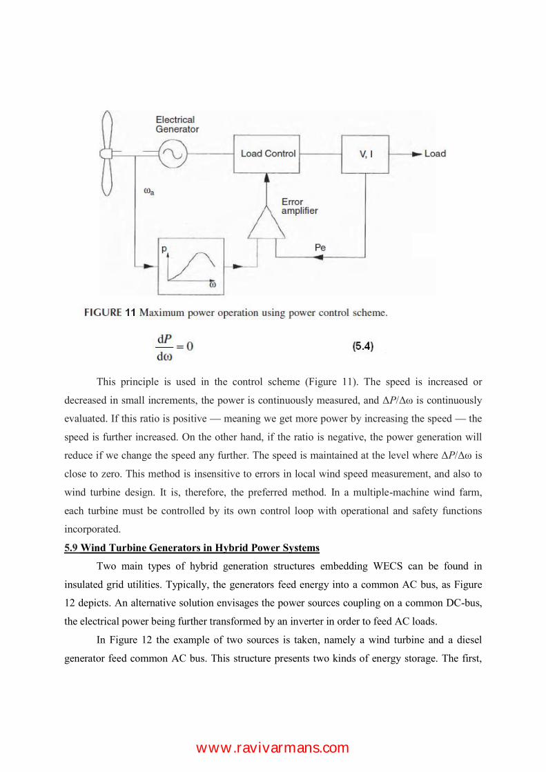
ΔΔω

— —

ΔΔω

www.ravivarmans.com

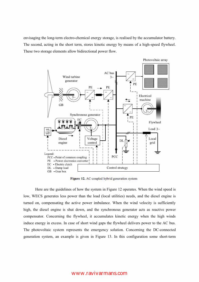
www.ravivarmans.com

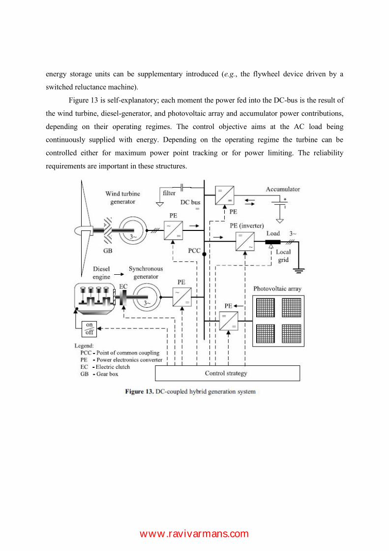
www.ravivarmans.com

Energy comparison of MPPT techniques for PV Systems

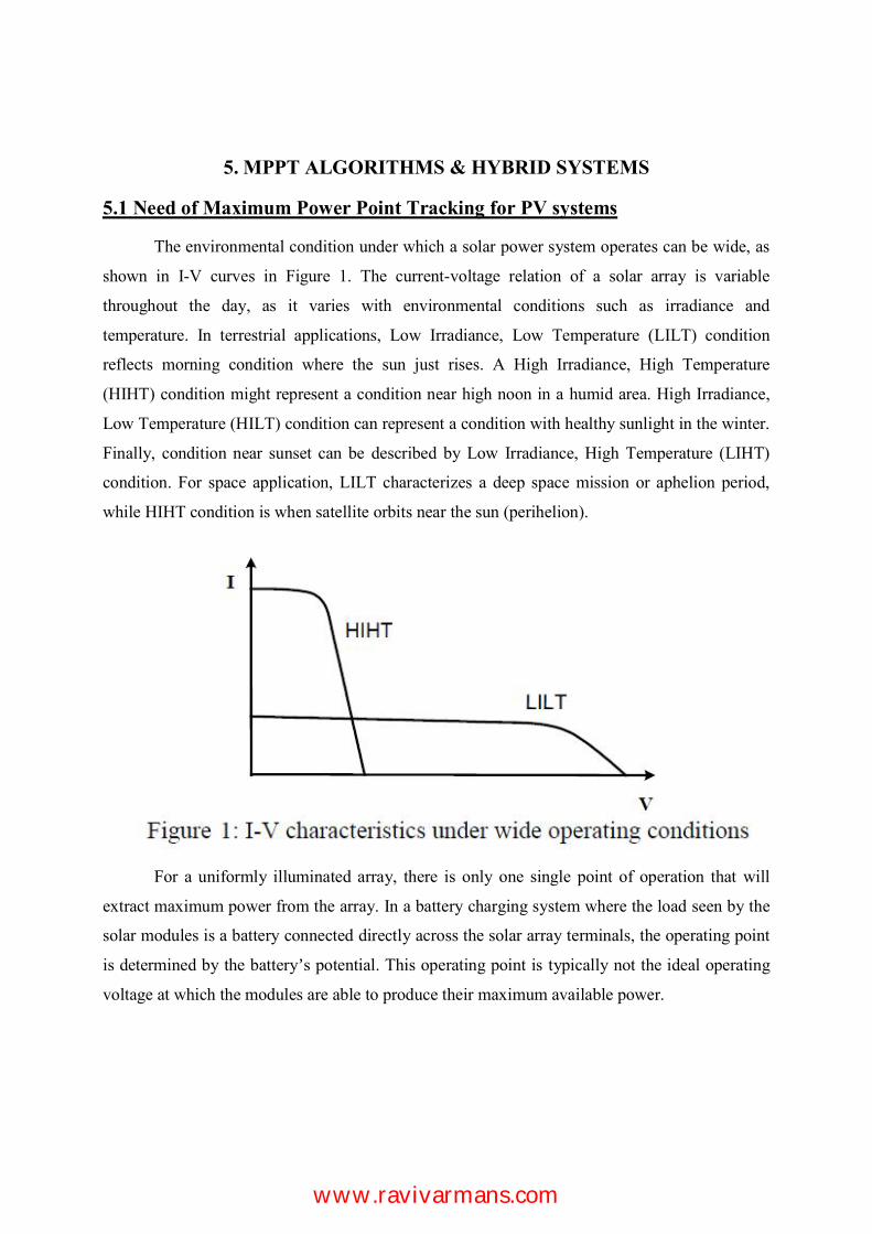
Abstract: - Many maximum power point tracking techniques for photovoltaic systems have been developed to maximize the produced energy and a lot of these are well established in the literature. These techniques vary in many aspects as: simplicity, convergence speed, digital or analogical implementation, sensors required, cost, range of effectiveness, and in other aspects. This paper presents a comparative study of ten widely-adopted MPPT algorithms; their performance is evaluated on the energy point of view, by using the simulation tool Simulink®, considering different solar irradiance variations. Key-Words: - Maximum power point (MPP), maximum power point tracking (MPPT), photovoltaic (PV), comparative study, PV Converter. 1 Introduction Solar energy is one of the most important renewable energy sources. As opposed to conventional unrenewable resources such as gasoline, coal, etc..., solar energy is clean, inexhaustible and free. The main applications of photovoltaic (PV) systems are in either stand-alone (water pumping, domestic and street lighting, electric vehicles, military and space applications) [1-2] or grid-connected configurations (hybrid systems, power plants) [3].

Unfortunately, PV generation systems have two major problems: the conversion efficiency of electric power generation is very low (9÷17%), especially under low irradiation conditions, and the amount of electric power generated by solar arrays changes continuously with weather conditions.

Moreover, the solar cell V-I characteristic is nonlinear and varies with irradiation and temperature. In general, there is a unique point on the V-I or V-P curve, called the Maximum Power Point (MPP), at which the entire PV system (array, converter, etc…) operates with maximum efficiency and produces its maximum output power. The location of the MPP is not known, but can be located, either through calculation models or by search algorithms. Therefore Maximum Power Point Tracking (MPPT) techniques are needed to maintain the PV array’s operating point at its MPP.

Many MPPT techniques have been proposed in the literature; examples are the Perturb and Observe (P&O) methods [4-7], the Incremental Conductance (IC) methods [4-8], the Artificial Neural Network method [9], the Fuzzy Logic method [10], etc...

These techniques vary between them in many aspects, including simplicity, convergence speed, hardware implementation, sensors required, cost, range of effectiveness and need for parameterization.

The P&O and IC techniques, as well as variants thereof, are the most widely used.

In this paper, ten MPPT algorithms are compared under the energy production point of view: P&O, modified P&O, Three Point Weight Comparison [12], Constant Voltage (CV) [13], IC, IC and CV combined [13], Short Current Pulse [14], Open Circuit Voltage [15], the Temperature Method [16] and methods derived from it [16]. These techniques are easily implemented and have been widely adopted for low-cost applications. Algorithms such as Fuzzy Logic, Sliding Mode [11], etc…, are beyond the scope of this paper, because they are more complex and less often used.

The MPPT techniques will be compared, by using Matlab tool Simulink®, created by MathWorks, considering different types of insulation and solar irradiance variations. The partially shaded condition will not be considered: the irradiation is assumed to be uniformly spread over the PV array.

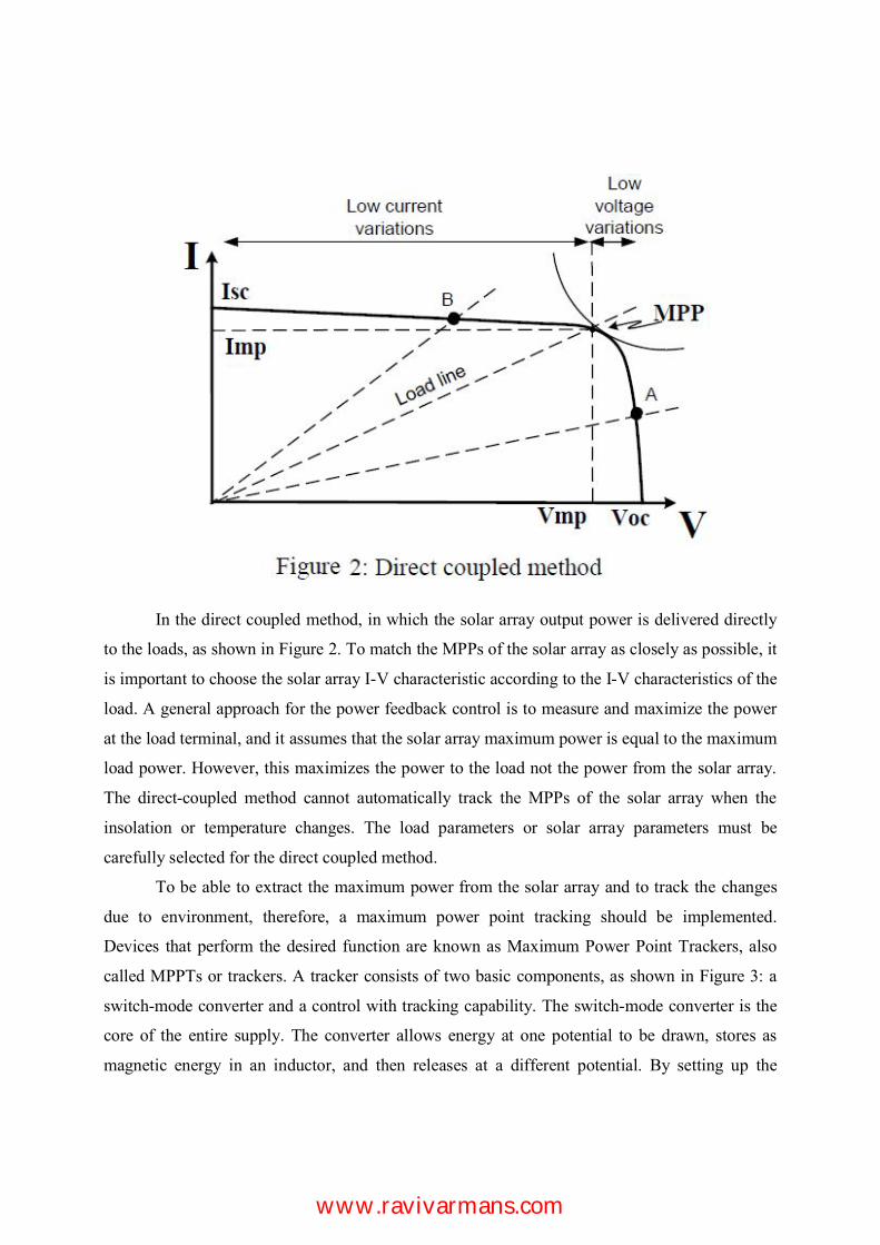
The PV system implementation takes into account the mathematical model of each component, as well as actual component specifications. In particular, without lack of generality, we will focus our attention on a stand-alone photovoltaic system constructed by connecting the dc/dc Single Ended Primary Inductor Converter (SEPIC) [17-18]

www.ravivarmans.com

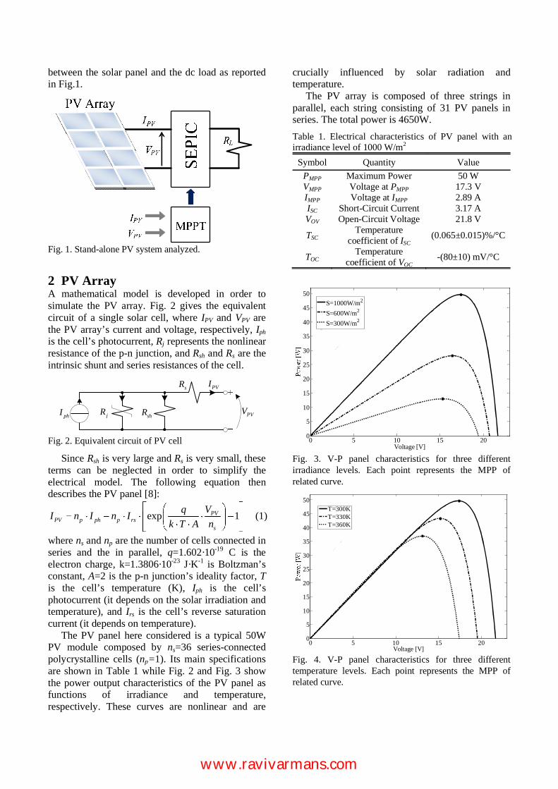
between the solar panel and the dc load as reported in Fig.1.

Fig. 1. Stand-alone PV system analyzed.

2 PV Array A mathematical model is developed in order to simulate the PV array. Fig. 2 gives the equivalent circuit of a single solar cell, where IPV and VPV are the PV array’s current and voltage, respectively, Iph is the cell’s photocurrent, Rj represents the nonlinear resistance of the p-n junction, and Rsh and Rs are the intrinsic shunt and series resistances of the cell.

phI shR

sR PVI

PVVjR

Fig. 2. Equivalent circuit of PV cell

Since Rsh is very large and Rs is very small, these terms can be neglected in order to simplify the electrical model. The following equation then describes the PV panel [8]:

exp 1PVPV p ph p rs

s

VqI n I n Ik T A n

(1)

where ns and np are the number of cells connected in series and the in parallel, q=1.602·10-19 C is the electron charge, k=1.3806·10-23 J·K-1 is Boltzman’s constant, A=2 is the p-n junction’s ideality factor, T is the cell’s temperature (K), Iph is the cell’s photocurrent (it depends on the solar irradiation and temperature), and Irs is the cell’s reverse saturation current (it depends on temperature).

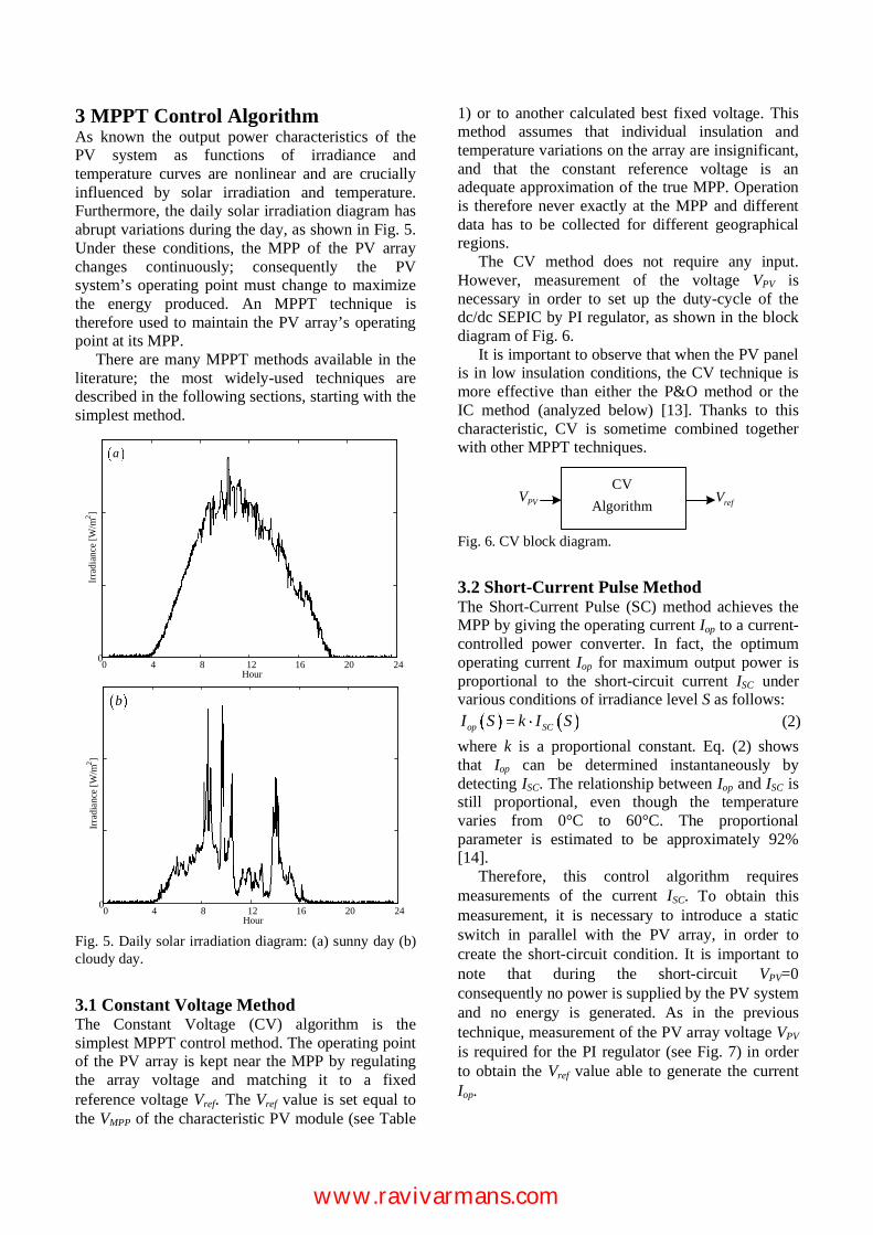
The PV panel here considered is a typical 50W PV module composed by ns=36 series-connected polycrystalline cells (np=1). Its main specifications are shown in Table 1 while Fig. 2 and Fig. 3 show the power output characteristics of the PV panel as functions of irradiance and temperature, respectively. These curves are nonlinear and are

crucially influenced by solar radiation and temperature.

The PV array is composed of three strings in parallel, each string consisting of 31 PV panels in series. The total power is 4650W. Table 1. Electrical characteristics of PV panel with an irradiance level of 1000 W/m2

Symbol Quantity Value PMPP Maximum Power 50 W VMPP Voltage at PMPP 17.3 V IMPP Voltage at IMPP 2.89 A ISC Short-Circuit Current 3.17 A VOV Open-Circuit Voltage 21.8 V

TSC Temperature coefficient of ISC (0.065±0.015)%/°C

TOC Temperature coefficient of VOC -(80±10) mV/°C

0 5 10 15 200

5

10

15

20

25

30

35

40

45

50

Voltage [V]

S=1000W/m2 S=600W/m2 S=300W/m2

data5data6

Fig. 3. V-P panel characteristics for three different irradiance levels. Each point represents the MPP of related curve.

0 5 10 15 200

5

10

15

20

25

30

35

40

45

50

Voltage [V]

T=300KT=330KT=360Kdata4data5data6

Fig. 4. V-P panel characteristics for three different temperature levels. Each point represents the MPP of related curve.

www.ravivarmans.com

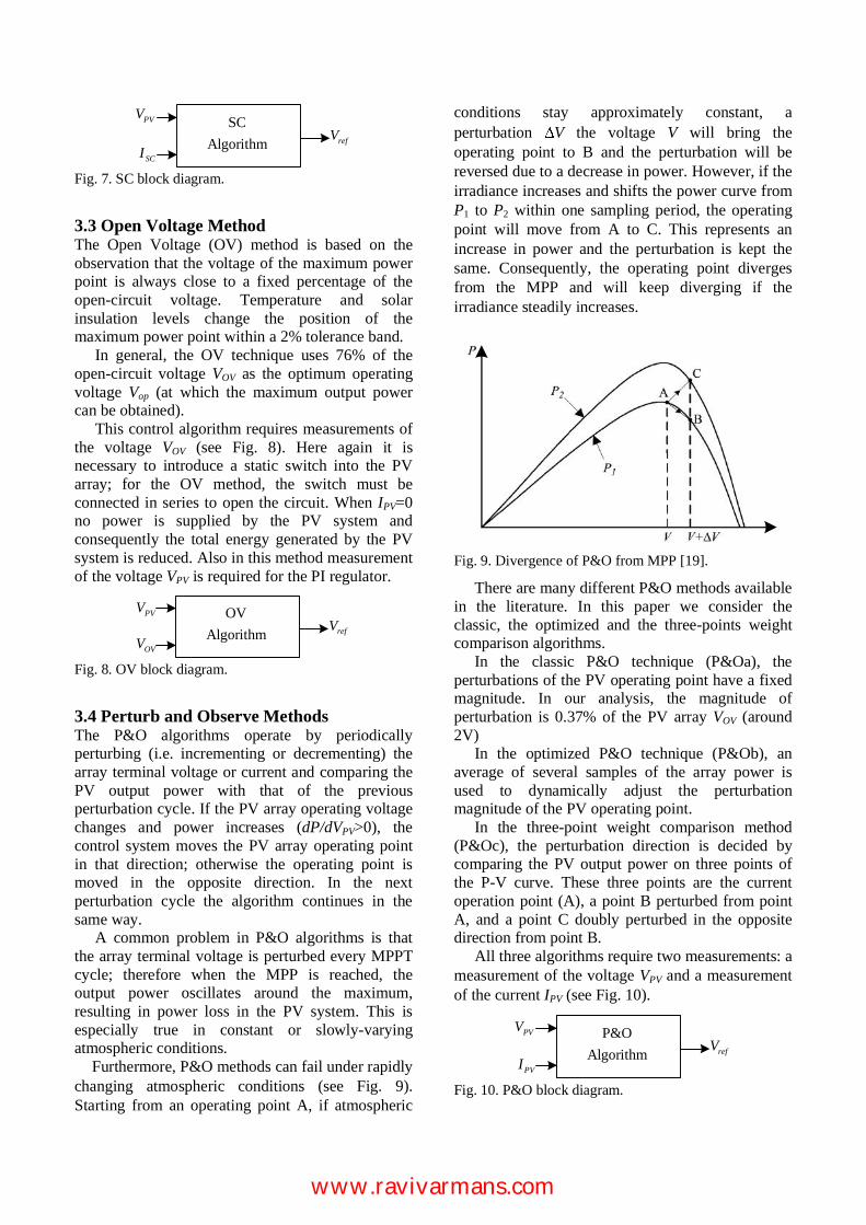
3 MPPT Control Algorithm As known the output power characteristics of the PV system as functions of irradiance and temperature curves are nonlinear and are crucially influenced by solar irradiation and temperature. Furthermore, the daily solar irradiation diagram has abrupt variations during the day, as shown in Fig. 5. Under these conditions, the MPP of the PV array changes continuously; consequently the PV system’s operating point must change to maximize the energy produced. An MPPT technique is therefore used to maintain the PV array’s operating point at its MPP.

There are many MPPT methods available in the literature; the most widely-used techniques are described in the following sections, starting with the simplest method.

0 4 8 12 16 20 240Hour

Irra

dian

ce [W

/m2 ]

0 4 8 12 16 20 240Hour

Irrad

ianc

e [W

/m2 ]

a

b

Fig. 5. Daily solar irradiation diagram: (a) sunny day (b) cloudy day.

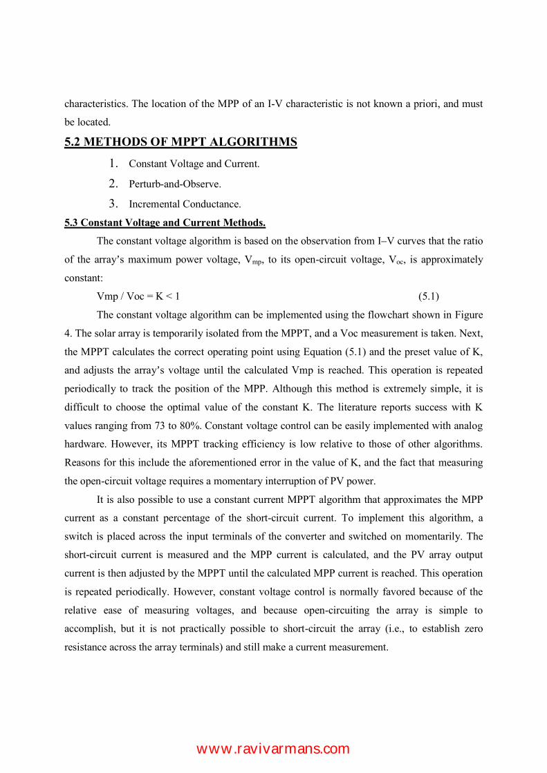
3.1 Constant Voltage Method The Constant Voltage (CV) algorithm is the simplest MPPT control method. The operating point of the PV array is kept near the MPP by regulating the array voltage and matching it to a fixed reference voltage Vref. The Vref value is set equal to the VMPP of the characteristic PV module (see Table

1) or to another calculated best fixed voltage. This method assumes that individual insulation and temperature variations on the array are insignificant, and that the constant reference voltage is an adequate approximation of the true MPP. Operation is therefore never exactly at the MPP and different data has to be collected for different geographical regions.

The CV method does not require any input. However, measurement of the voltage VPV is necessary in order to set up the duty-cycle of the dc/dc SEPIC by PI regulator, as shown in the block diagram of Fig. 6.

It is important to observe that when the PV panel is in low insulation conditions, the CV technique is more effective than either the P&O method or the IC method (analyzed below) [13]. Thanks to this characteristic, CV is sometime combined together with other MPPT techniques.

CVAlgorithm refVPVV

Fig. 6. CV block diagram.

3.2 Short-Current Pulse Method The Short-Current Pulse (SC) method achieves the MPP by giving the operating current Iop to a current-controlled power converter. In fact, the optimum operating current Iop for maximum output power is proportional to the short-circuit current ISC under various conditions of irradiance level S as follows:

op SCI S k I S (2) where k is a proportional constant. Eq. (2) shows that Iop can be determined instantaneously by detecting ISC. The relationship between Iop and ISC is still proportional, even though the temperature varies from 0°C to 60°C. The proportional parameter is estimated to be approximately 92% [14].

Therefore, this control algorithm requires measurements of the current ISC. To obtain this measurement, it is necessary to introduce a static switch in parallel with the PV array, in order to create the short-circuit condition. It is important to note that during the short-circuit VPV=0 consequently no power is supplied by the PV system and no energy is generated. As in the previous technique, measurement of the PV array voltage VPV is required for the PI regulator (see Fig. 7) in order to obtain the Vref value able to generate the current Iop.

www.ravivarmans.com

SCAlgorithm refV

SCI

PVV

Fig. 7. SC block diagram.

3.3 Open Voltage Method The Open Voltage (OV) method is based on the observation that the voltage of the maximum power point is always close to a fixed percentage of the open-circuit voltage. Temperature and solar insulation levels change the position of the maximum power point within a 2% tolerance band.

In general, the OV technique uses 76% of the open-circuit voltage VOV as the optimum operating voltage Vop (at which the maximum output power can be obtained).

This control algorithm requires measurements of the voltage VOV (see Fig. 8). Here again it is necessary to introduce a static switch into the PV array; for the OV method, the switch must be connected in series to open the circuit. When IPV=0 no power is supplied by the PV system and consequently the total energy generated by the PV system is reduced. Also in this method measurement of the voltage VPV is required for the PI regulator.

OVAlgorithm refV

OVV

PVV

Fig. 8. OV block diagram.

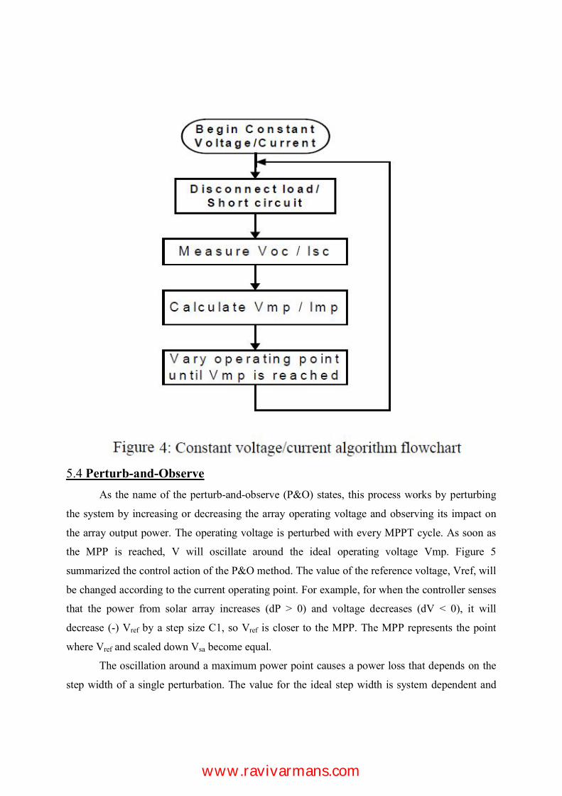
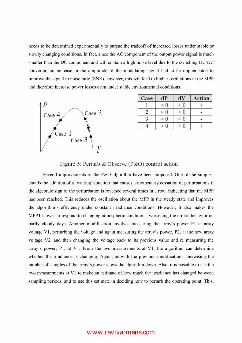
3.4 Perturb and Observe Methods The P&O algorithms operate by periodically perturbing (i.e. incrementing or decrementing) the array terminal voltage or current and comparing the PV output power with that of the previous perturbation cycle. If the PV array operating voltage changes and power increases (dP/dVPV>0), the control system moves the PV array operating point in that direction; otherwise the operating point is moved in the opposite direction. In the next perturbation cycle the algorithm continues in the same way.

A common problem in P&O algorithms is that the array terminal voltage is perturbed every MPPT cycle; therefore when the MPP is reached, the output power oscillates around the maximum, resulting in power loss in the PV system. This is especially true in constant or slowly-varying atmospheric conditions.

Furthermore, P&O methods can fail under rapidly changing atmospheric conditions (see Fig. 9). Starting from an operating point A, if atmospheric

conditions stay approximately constant, a perturbation V the voltage V will bring the operating point to B and the perturbation will be reversed due to a decrease in power. However, if the irradiance increases and shifts the power curve from P1 to P2 within one sampling period, the operating point will move from A to C. This represents an increase in power and the perturbation is kept the same. Consequently, the operating point diverges from the MPP and will keep diverging if the irradiance steadily increases.

Fig. 9. Divergence of P&O from MPP [19].

There are many different P&O methods available in the literature. In this paper we consider the classic, the optimized and the three-points weight comparison algorithms.

In the classic P&O technique (P&Oa), the perturbations of the PV operating point have a fixed magnitude. In our analysis, the magnitude of perturbation is 0.37% of the PV array VOV (around 2V)

In the optimized P&O technique (P&Ob), an average of several samples of the array power is used to dynamically adjust the perturbation magnitude of the PV operating point.

In the three-point weight comparison method (P&Oc), the perturbation direction is decided by comparing the PV output power on three points of the P-V curve. These three points are the current operation point (A), a point B perturbed from point A, and a point C doubly perturbed in the opposite direction from point B.

All three algorithms require two measurements: a measurement of the voltage VPV and a measurement of the current IPV (see Fig. 10).

P&OAlgorithm refV

PVI

PVV

Fig. 10. P&O block diagram.

www.ravivarmans.com

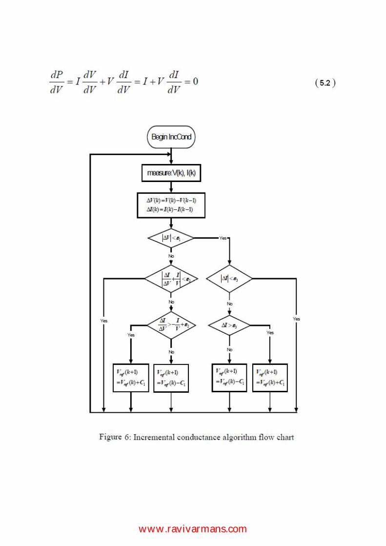
3.5 Incremental Conductance Methods The Incremental Conductance (IC) algorithm is based on the observation that the following equation holds at the MPP [4]:

0PV PV

PV PV

dI IdV V

(3)

where IPV and VPV are the PV array current and voltage, respectively.

When the optimum operating point in the P-V plane is to the right of the MPP, we have (dIPV/dVPV)+(IPV/VPV)<0, whereas when the optimum operating point is to the left of the MPP, we have (dIPV/dVPV)+(IPV/VPV)>0.

The MPP can thus be tracked by comparing the instantaneous conductance IPV/VPV to the incremental conductance dIPV/dVPV. Therefore the sign of the quantity (dIPV/dVPV)+(IPV/VPV) indicates the correct direction of perturbation leading to the MPP. Once MPP has been reached, the operation of PV array is maintained at this point and the perturbation stopped unless a change in dIPV is noted. In this case, the algorithm decrements or increments Vref to track the new MPP. The increment size determines how fast the MPP is tracked.

Through the IC algorithm it is therefore theoretically possible to know when the MPP has been reached, and thus when the perturbation can be stopped. The IC method offers good performance under rapidly changing atmospheric conditions.

There are two main different IC methods available in the literature.

The classic IC algorithm (ICa) requires the same measurements shown in Fig.10, in order to determine the perturbation direction: a measurement of the voltage VPV and a measurement of the current IPV.

The Two-Model MPPT Control (ICb) algorithm combines the CV and the ICa methods: if the irradiation is lower than 30% of the nominal irradiance level the CV method is used, other way the ICa method is adopted. Therefore this method requires the additional measurement of solar irradiation S as shown in Fig. 11.

ICbAlgorithm refV

PVI

PVV

S

Fig. 11. ICb block diagram.

3.6 Temperature Methods The open-circuit voltage VOV of the solar cell varies mainly with the cell temperature, whereas the short-circuit current is directly proportional to the irradiance level (Fig. 12), and is relatively steady over cell temperature changes (Fig. 13).

The open-circuit voltage VOV can be described through the following equation [16]:

OVOV OVSTC STC

dVV V T T

dT (4)

where VOVSTC=21.8V is the open-circuit voltage under Standard Test Conditions (STC), (dVOV/dT)=-0.08V/K is the temperature gradient, and TSTC is the cell temperature under STC. On the other hand, the MPP voltage, VMPP, in any operating condition can be described through the following equation:

_MPP MPP STCV u S v T w S y V (5) where VMPP_STC is the MPP voltage under STC. Table 2 shows the parameters of the optimal voltage equation (5) in relation to the irradiance level S.

0 5 10 15 20 250

0.5

1

1.5

2

2.5

3

3.5

Voltage [V]

S=600 W/m2

S=300 W/m2

S=1000 W/m2

Fig. 12. V-I characteristics for three different irradiance levels.

0 5 10 15 20 250

0.5

1

1.5

2

2.5

3

3.5

Voltage [V]

T=300KT=330KT=360K

Fig. 13. V-I characteristics for three different temperatures.

There are two different temperature methods available in the literature.

The Temperature Gradient (TG) algorithm uses

www.ravivarmans.com

the temperature T to determine the open-circuit voltage VOV from equation (4). The MPP voltage VMPP is then determined as in the OV technique, avoiding power losses. TG requires the measurement of the temperature T and a measurement of the voltage VPV for the PI regulator (see Fig. 14 a).

Table 2. Parameters of the optimal voltage equation S

(kW/m2) u(S) v(S) w(S) y(S)

0.1÷0.2 0.43404 0.1621 0.00235 -6e-4 0.2÷0.3 0.45404 0.0621 0.00237 -7e-4 0.3÷0.4 0.46604 0.0221 0.00228 -4e-4 0.4÷0.5 0.46964 0.0131 0.00224 -3e-4 0.5÷0.6 0.47969 -0.0070 0.00224 -3e-4 0.6÷0.7 0.48563 -0.0169 0.00218 -2e-4 0.7÷0.8 0.49270 -0.0270 0.00239 -5e-4 0.8÷0.9 0.49190 -0.0260 0.00223 -3e-4 0.9÷1.0 0.49073 -0.0247 0.00205 -1e-4

TMAlgorithm refV

T

PVV

(a)

TPAlgorithm refV

T

PVVS

(b)

Fig. 14. (a) TM block diagram; (b) TP block diagram.

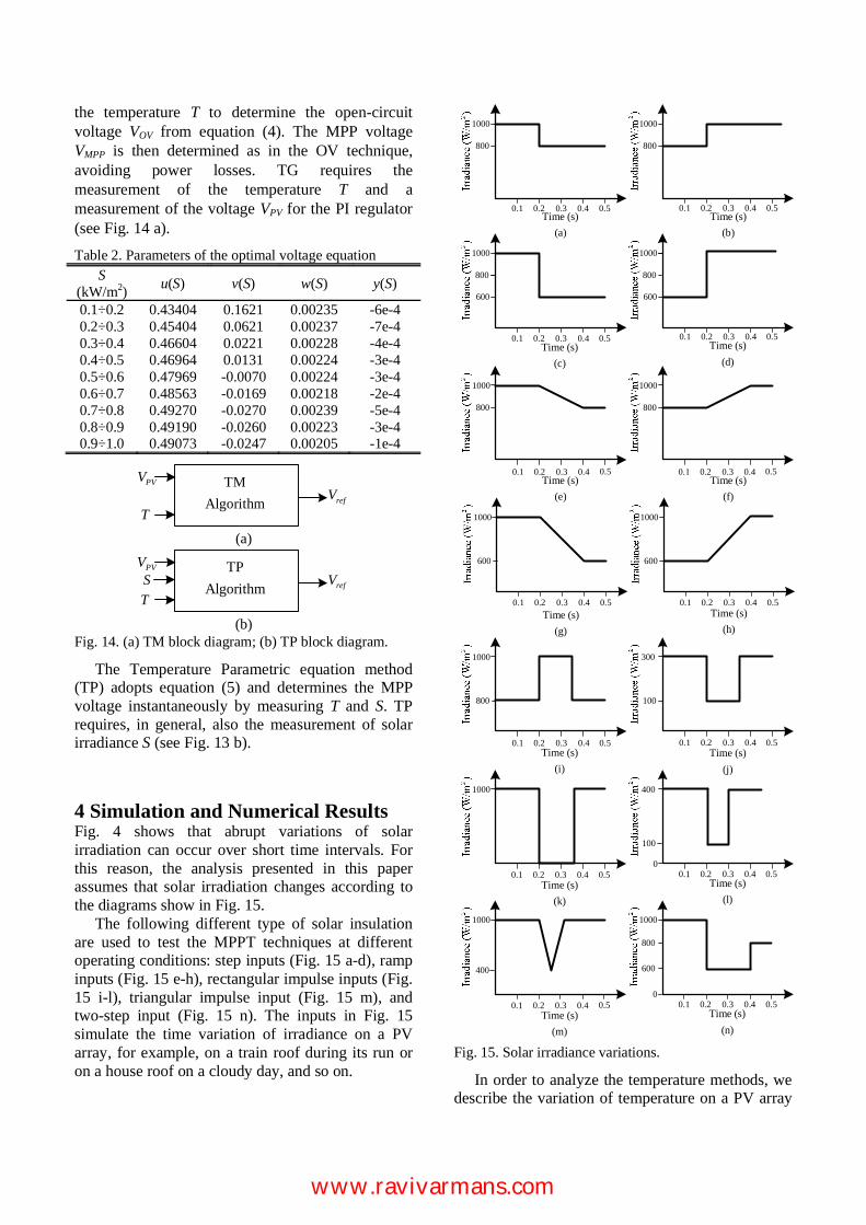
The Temperature Parametric equation method (TP) adopts equation (5) and determines the MPP voltage instantaneously by measuring T and S. TP requires, in general, also the measurement of solar irradiance S (see Fig. 13 b). 4 Simulation and Numerical Results Fig. 4 shows that abrupt variations of solar irradiation can occur over short time intervals. For this reason, the analysis presented in this paper assumes that solar irradiation changes according to the diagrams show in Fig. 15.

The following different type of solar insulation are used to test the MPPT techniques at different operating conditions: step inputs (Fig. 15 a-d), ramp inputs (Fig. 15 e-h), rectangular impulse inputs (Fig. 15 i-l), triangular impulse input (Fig. 15 m), and two-step input (Fig. 15 n). The inputs in Fig. 15 simulate the time variation of irradiance on a PV array, for example, on a train roof during its run or on a house roof on a cloudy day, and so on.

1000

Time (s)(a)

800

0.1 0.2 0.3 0.4 0.5

1000

800

1000

600

Time (s)(b)

Time (s)(c)

Time (s)(d)

Time (s)(e)

Time (s)(f)

Time (s)(i)

Time (s)(j)

400

Time (s)(k)

Time (s)(l)

800

1000

600

800

1000

800

1000

800

1000

800

300

100

1000

0

Time (s)(g)

Time (s)(h)

1000

600

1000

600

0.1 0.2 0.3 0.4 0.5

0.1 0.2 0.3 0.4 0.5 0.1 0.2 0.3 0.4 0.5

0.1 0.2 0.3 0.4 0.5 0.1 0.2 0.3 0.4 0.5

0.1 0.2 0.3 0.4 0.5 0.1 0.2 0.3 0.4 0.5

0.1 0.2 0.3 0.4 0.5 0.1 0.2 0.3 0.4 0.5

0.1 0.2 0.3 0.4 0.5 0.1 0.2 0.3 0.4 0.5

1000

Time (s)(m)

Time (s)(n)

1000

400

00.1 0.2 0.3 0.4 0.5 0.1 0.2 0.3 0.4 0.5

100

600

800

Fig. 15. Solar irradiance variations.

In order to analyze the temperature methods, we describe the variation of temperature on a PV array

www.ravivarmans.com

accordingly to the equivalent circuit shown in Fig. 16. If the temperature is uniformly distributed, the following differential equation can be used as temperature model [16]:

T dTS CR dt

(6)

where R=0.0435m2K/W is the thermal resistance and C=15.71·10-3J/m2K is the thermal capacitance.

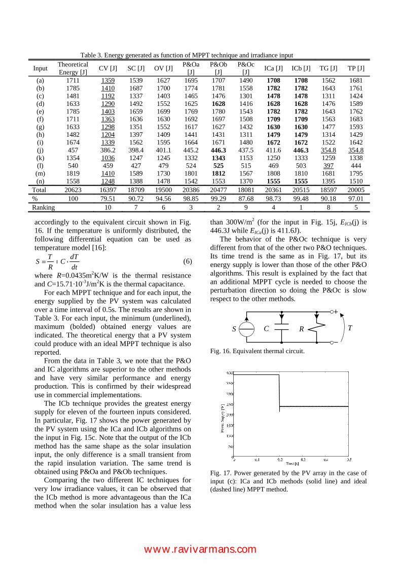
For each MPPT technique and for each input, the energy supplied by the PV system was calculated over a time interval of 0.5s. The results are shown in Table 3. For each input, the minimum (underlined), maximum (bolded) obtained energy values are indicated. The theoretical energy that a PV system could produce with an ideal MPPT technique is also reported.

From the data in Table 3, we note that the P&O and IC algorithms are superior to the other methods and have very similar performance and energy production. This is confirmed by their widespread use in commercial implementations.

The ICb technique provides the greatest energy supply for eleven of the fourteen inputs considered. In particular, Fig. 17 shows the power generated by the PV system using the ICa and ICb algorithms on the input in Fig. 15c. Note that the output of the ICb method has the same shape as the solar insulation input, the only difference is a small transient from the rapid insulation variation. The same trend is obtained using P&Oa and P&Ob techniques.

Comparing the two different IC techniques for very low irradiance values, it can be observed that the ICb method is more advantageous than the ICa method when the solar insulation has a value less

than 300W/m2 (for the input in Fig. 15j, EICb(j) is 446.3J while EICa(j) is 411.6J).

Table 3. Energy generated as function of MPPT technique and irradiance input P&Oa

[J] P&Ob

[J] P&Oc

[J] Theoretical ICa [J] ICb [J] TG [J] TP [J] CV [J] SC [J] OV [J] Input Energy [J]

1708 1708 (a) 1711 1359 1539 1627 1695 1707 1490 1562 1681

1782 1782 (b) 1785 1410 1687 1700 1774 1781 1558 1643 1761

1478 1478 (c) 1481 1192 1337 1403 1465 1476 1301 1311 1424

1628 1628 1628 (d) 1633 1290 1492 1552 1625 1416 1476 1589

1782 1782 (e) 1785 1403 1659 1699 1769 1780 1543 1643 1762

1709 1709 (f) 1711 1363 1636 1630 1692 1697 1508 1563 1683

1630 1630 (g) 1633 1298 1351 1552 1617 1627 1432 1477 1593

1479 1479

The behavior of the P&Oc technique is very different from that of the other two P&O techniques. Its time trend is the same as in Fig. 17, but its energy supply is lower than those of the other P&O algorithms. This result is explained by the fact that an additional MPPT cycle is needed to choose the perturbation direction so doing the P&Oc is slow respect to the other methods.

S R TC

Fig. 16. Equivalent thermal circuit.

Fig. 17. Power generated by the PV array in the case of input (c): ICa and ICb methods (solid line) and ideal (dashed line) MPPT method.

(h) 1482 1204 1397 1409 1441 1431 1311 1314 1429

1672 1672 (i) 1674 1339 1562 1595 1664 1671 1480 1522 1642

446.3 446.3 (j) 457 386.2 398.4 401.1 445.2 437.5 411.6 354.8 354.8

1343 (k) 1354 1036 1247 1245 1332 1153 1250 1333 1259 1338

(l) 540 459 427 479 524 525 515 469 503 397 444

1812 (m) 1819 1410 1589 1730 1801 1567 1808 1810 1681 1795

1555 1555 (n) 1558 1248 1388 1478 1542 1553 1370 1395 1510

Total 20623 16397 18709 19500 20386 20477 18081 20361 20515 18597 20005 % 100 79.51 90.72 94.56 98.85 99.29 87.68 98.73 99.48 90.18 97.01 Ranking 10 7 6 3 2 9 4 1 8 5

www.ravivarmans.com

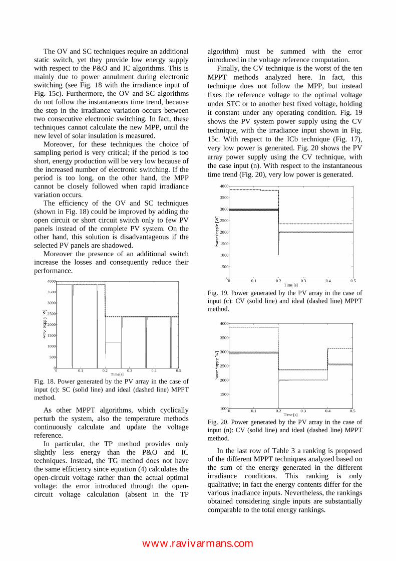
The OV and SC techniques require an additional static switch, yet they provide low energy supply with respect to the P&O and IC algorithms. This is mainly due to power annulment during electronic switching (see Fig. 18 with the irradiance input of Fig. 15c). Furthermore, the OV and SC algorithms do not follow the instantaneous time trend, because the step in the irradiance variation occurs between two consecutive electronic switching. In fact, these techniques cannot calculate the new MPP, until the new level of solar insulation is measured.

Moreover, for these techniques the choice of sampling period is very critical; if the period is too short, energy production will be very low because of the increased number of electronic switching. If the period is too long, on the other hand, the MPP cannot be closely followed when rapid irradiance variation occurs.

The efficiency of the OV and SC techniques (shown in Fig. 18) could be improved by adding the open circuit or short circuit switch only to few PV panels instead of the complete PV system. On the other hand, this solution is disadvantageous if the selected PV panels are shadowed.

Moreover the presence of an additional switch increase the losses and consequently reduce their performance.

0 0.1 0.2 0.3 0.4 0.50

500

1000

1500

2000

2500

3000

3500

4000

Time[s] Fig. 18. Power generated by the PV array in the case of input (c): SC (solid line) and ideal (dashed line) MPPT method.

As other MPPT algorithms, which cyclically perturb the system, also the temperature methods continuously calculate and update the voltage reference.

In particular, the TP method provides only slightly less energy than the P&O and IC techniques. Instead, the TG method does not have the same efficiency since equation (4) calculates the open-circuit voltage rather than the actual optimal voltage: the error introduced through the open-circuit voltage calculation (absent in the TP

algorithm) must be summed with the error introduced in the voltage reference computation.

Finally, the CV technique is the worst of the ten MPPT methods analyzed here. In fact, this technique does not follow the MPP, but instead fixes the reference voltage to the optimal voltage under STC or to another best fixed voltage, holding it constant under any operating condition. Fig. 19 shows the PV system power supply using the CV technique, with the irradiance input shown in Fig. 15c. With respect to the ICb technique (Fig. 17), very low power is generated. Fig. 20 shows the PV array power supply using the CV technique, with the case input (n). With respect to the instantaneous time trend (Fig. 20), very low power is generated.

0 0.1 0.2 0.3 0.4 0.50

500

1000

1500

2000

2500

3000

3500

4000

Time [s] Fig. 19. Power generated by the PV array in the case of input (c): CV (solid line) and ideal (dashed line) MPPT method.

0 0.1 0.2 0.3 0.4 0.51000

1500

2000

2500

3000

3500

4000

Time [s] Fig. 20. Power generated by the PV array in the case of input (n): CV (solid line) and ideal (dashed line) MPPT method.

In the last row of Table 3 a ranking is proposed of the different MPPT techniques analyzed based on the sum of the energy generated in the different irradiance conditions. This ranking is only qualitative; in fact the energy contents differ for the various irradiance inputs. Nevertheless, the rankings obtained considering single inputs are substantially comparable to the total energy rankings.

www.ravivarmans.com

5 Costs Comparison To complete our analysis a simple discussion about the cost of the MPPT technique is presented [20]. A satisfactory MPPT costs comparison can be carried out by knowing the technique (analogical or digital) adopted in the control device, the number of sensors, and the use of additional power component, considering the other costs (power components, electronic components, boards, etc…) equal for all the devices.

The MPPT implementation typology greatly depends on the end-users’ knowledge, with analogical circuit, SC, OV, or CV are good options, otherwise with digital circuit that require the use of microcontroller, P&O, IC, and temperature methods are enough easily to implement. Moreover it is important to underline that analogical implementations are generally cheaper than digital (the microcontroller and relative program are expensive). To make all the cost comparable between them, the computation cost comparison is formulated taking into account the present spread of MPPT methods.

The number of sensors required to implement the MPPT technique also affects the final costs. Most of the time, it is easier and more reliable to measure voltage than current and the current sensors are usually more expensive and bulky. The irradiance or temperature sensors are very expensive and uncommon.

After these considerations, Table 4 proposes a simplified classification considering the costs of sensors, microcontroller and the additional power components.

Table 4. Cost evaluation. (A=absent, L=low, M=medium, H=high)

COST

MPPT Additional

power component

Sensor Microcontroller computation Total

CV A L A/L L SC H M A/L M OV H L/M A/L L/M

P&Oa A M L L/M P&Ob A M L L/M P&Oc A M M M

ICa A M M M ICb A H M/H H TG A M/H M M/H TP A H M/H H

6 Conclusion This paper has presented a comparison among ten different Maximum Power Point Tracking techniques in relation to their performance and implementation costs. In particular, fourteen different types of solar insulation are considered, and the energy supplied by a complete PV array is calculated; furthermore, regarding the MPPT implementation costs, a cost comparison is proposed taking into consideration the costs of sensors, microcontroller and additional power components.

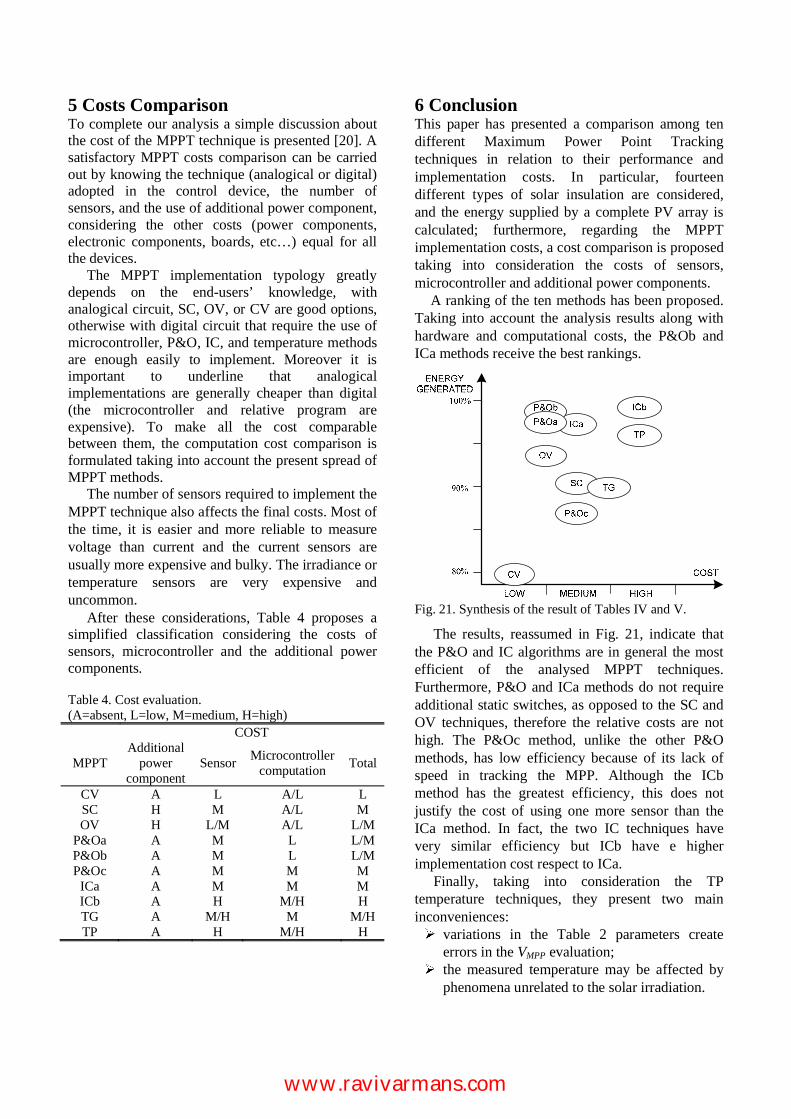
A ranking of the ten methods has been proposed. Taking into account the analysis results along with hardware and computational costs, the P&Ob and ICa methods receive the best rankings.

Fig. 21. Synthesis of the result of Tables IV and V.

The results, reassumed in Fig. 21, indicate that the P&O and IC algorithms are in general the most efficient of the analysed MPPT techniques. Furthermore, P&O and ICa methods do not require additional static switches, as opposed to the SC and OV techniques, therefore the relative costs are not high. The P&Oc method, unlike the other P&O methods, has low efficiency because of its lack of speed in tracking the MPP. Although the ICb method has the greatest efficiency, this does not justify the cost of using one more sensor than the ICa method. In fact, the two IC techniques have very similar efficiency but ICb have e higher implementation cost respect to ICa.

Finally, taking into consideration the TP temperature techniques, they present two main inconveniences:

variations in the Table 2 parameters create errors in the VMPP evaluation; the measured temperature may be affected by

phenomena unrelated to the solar irradiation.

www.ravivarmans.com

Further research on this subject should focus on experimental comparisons between these techniques, especially under shadow conditions. References: [1] S. Leva, D. Zaninelli, Technical and Financial

Analysis for Hybrid Photovoltaic Power Generation Systems, WSEAS Transactions on Power Systems, vol.5, no.1, May 2006, pp.831-838

[2] S. Leva, D. Zaninelli, R. Contino, Integrated renewable sources for supplying remote power systems, WSEAS Transactions on Power Systems, vol.2, no.2, February 2007, pp.41-48

[3] J.Schaefer, Review of Photovoltaic Power Plant Performance and Economics, IEEE Trans. Energy Convers., vol. EC-5,pp. 232-238, June, 1990.

[4] N.Femia, D.Granozio, G.Petrone, G.Spaguuolo, M.Vitelli, Optimized One-Cycle Control in Photovoltaic Grid Connected Applications, IEEE Trans. Aerosp. Electron. Syst., vol. 2, no 3, July 2006.

[5] W. Wu, N. Pongratananukul, W. Qiu, K. Rustom, T. Kasparis and I. Batarseh, DSP-based Multiple Peack Power Tracking for Expandable Power System, Proc. APEC, 2003, pp. 525-530.

[6] C. Hua and C. Shen, Comparative Study of Peak Power Tracking Techniques for Solar Storage System, Proc. APEC, 1998, pp. 679-685.

[7] D.P.Hohm and M.E.Ropp, Comparative Study of Maximum Power Point Tracking Algorithms Using an Experimental, Programmable, Maximum Power Point Tracking Test Bed, Proc. Photovoltaic Specialist Conference, 2000, pp. 1699-1702.

[8] K.H.Hussein, I.Muta, T.Hoshino and M.osakada Maximum Power Point Tracking: an Algorithm for Rapidly Chancing Atmospheric Conditions, IEE Proc.-Gener. Transm. Distrib., vol. 142, no.1, pp. 59-64, January, 1995.

[9] X.Sun, W.Wu, Xin Li and Q.Zhao, A Research on Photovoltaic Energy Controlling System with Maximum Power Point Tracking, Power Conversion Conference, 2002, pp. 822-826.

[10]T.L. Kottas, Y.S.Boutalis and A. D. Karlis, New Maximum Power Point Tracker for PV Arrays Using Fuzzy Controller in Close Cooperation with Fuzzy Cognitive Network, IEEE Trans. Energy Conv., vol.21, no.3, 2006.

[11]A. El Jouni, R. El-Bachtiri and J. Boumhidi, Sliding Mode Controller for the Maximum

Power Point Tracking of a Photovoltaic Pumping System, WSEAS Transactions on Power Systems, vol.1, no.10, pp. 1675-1680, 2006.

[12]Y.T.Hsiao and C.H.Chen, Maximum Power Tracking for Photovoltaic Power System, Proc. Industry Application Conference, 2002, pp. 1035-1040.

[13]G.J.Yu, Y.S.Jung, J.Y.Choi, I.Choy, J.H.Song and G.S.Kim, A Novel Two-Mode MPPT Control Algorithm Based on Comparative Study of Existing Algorithms, Proc. Photovoltaic Specialists Conference, 2002, pp. 1531-1534.

[14]T.Noguchi, S.Togashi and R.Nakamoto, Short-Current Pulse-Based Maximum-Power-Point Tracking Method for Multiple Photovoltaic-and-Converter Module System, IEEE Trans. Ind. Electron., vol.49, no.1, pp. 217-223, 2002.

[15]D.Y. Lee, H.J. Noh, D.S. Hyun and I.Choy, An Improved MPPT Converter Using Current Compensation Method for Small Scaled PV-Applications, Proc. APEC, 2003, pp.540-545.

[16]M.Park and I.K. Yu, A Study on Optimal Voltage for MPPT Obtained by Surface Temperature of Solar Cell, Proc. IECON, 2004, pp. 2040-2045.

[17]F. Castelli Dezza, M. Diforte, R. Faranda, Control strategy for a single phase solution able to improve power quality in DG applications, Proc. PELINCEC, 2005

[18]F. Castelli Dezza, M. Diforte, R. Faranda, A solar converter for distributed generation able to improve the power quality supply, Proc. 18th International Conference on Electricity Distribution, Turin (Italy), June 2005

[19]O. Wasynczuk, Dynamic behavior of a class of photovoltaic power systems, IEEE Trans. Power App. Syst., vol. 102, no. 9, pp. 3031–3037, Sep. 1983

[20]T. Esram, and P.L. Chapman, Comparison of Photovoltaic Array Maximum Power Point Tracking Techniques, IEEE Trans. Energy Conv., vol.22, no.2, June, 2007, pp.439-449

www.ravivarmans.com